G16.4427 Practical MRI 1 – 19 th February 2015 G16.4427 Practical MRI 1 Gradients

G16.4427 Practical MRI 1 – 19th February 2015

G16.4427 Practical MRI 1

Gradients


The Gradients

http://www.cis.rit.edu/htbooks/mri/


The Gradients• Role– Select excited volumes– Encode spatial information

• Important components and parameters– Components: gradient coils, gradient amplifiers– Parameters: gradient strength, slew rate,

homogeneity volume, length• Impact– Increased imaging speed/efficiency– Improved velocity and diffusion encoding– Short TE/TR


The Gradient Coils

B0

∆B“Fast” spins “Slow” spins

Lauterbur & MansfieldNobel Prize in Physiology or Medicine, 2003


X, Y and Z Gradient Coils


Modern Gradient Coils


Introduction• In MRI, magnetic field gradients refer to the spatial

variation of the z component of the magnetic field:


Introduction• In MRI, magnetic field gradients refer to the spatial variation of

the z component of the magnetic field:

• Gradient amplitudes are typically measured in mT/m or G/cm (10 mT/m = 1 G/cm)

• When a gradient driver produces its maximal current, its associated coil produces its maximal gradient strength (h)

• When a gradient driver produces its maximal voltage, the amplitude of the associated gradient field undergoes its largest rate of change, called the maximum gradient slew rate (SR)

• Typical values for whole-body gradient systems are h ~ 10-50 mT/m and SR ~ 10-200 T/m/s


Useful Definitions• The product hSR ( max power) is a measure of ∝

the gradient system’s performance– Limit on dB/dt to avoid peripheral nerve stimulation


Useful Definitions• The product hSR ( max power) is a measure of ∝

the gradient system’s performance– Limit on dB/dt to avoid peripheral nerve stimulation– Limit on duty cycle to avoid thermal heating

• With linear ramps, the rise time is r = h/SR

• Gradient lobe refer to a single gradient pulse shape that starts and ends with zero amplitude– Examples of lobes include triangles and trapezoids

• Gradient waveform refers to all gradient lobes on a single axis within a pulse sequence


Simple Gradient Lobes• The area A of a gradient lobe when plotted versus

time is typically determined by the prescribed imaging parameters (e.g. FOV, matrix size, BW)

• Often also the shape is determined by imaging constraints– The shortest duration gradient lobe is normally used in

order to minimize timing parameters such as TE and TR• For gradient systems that use linear ramps, the

simple lobe shapes with the shortest duration will be triangular or trapezoidal


Trapezoidal and Triangular Lobes

The ramps have maximal slope in both cases:

We select the most efficient shape based on the gradient area:

Triangle with

Trapezoid with

Bernstein et al. (2004) Handbook of MRI Pulse Sequences


Sinusoidal LobesA half-sine lobe that starts at t = t0 is given by:

Maximal slew rate is at its beginning and end:

The lobe area is:



Problem:Calculate the gradient amplitude and duration for a sinusoidal lobe

that satisfies both the gradient amplitude and slew-rate

constraints


Sinusoidal Lobes

Maximal slew rate is at its beginning and end:

The lobe area is:

The gradient amplitude that satisfies both the gradient amplitude and slew-rate constraints is:

A half-sine lobe that starts at t = t0 is given by:



Bridged Gradient Lobes

• Advantages:- more compact gradient waveform- rb is less than r1 + r2

- less acoustic noise- less gradient heating- less eddy currents

• The plateau of the second lobe must be increased to preserve the gradient area



Any questions?


Frequency Encoding Gradients• Frequency encoding is employed by many pulse sequences,

including projection acquisition and Fourier imaging• A frequency-encoding gradient can be applied along any

physical direction• The polarity of the frequency-encoding gradient can be

either positive or negative• The waveform typically consists of two portions, a

prephasing gradient lobe and a readout gradient lobe– The amplitude and duration of the readout gradient lobe are

related to image resolution, receiver BW, FOV and γ– In multi-echo pulse sequences (e.g. EPI) the second half of the

readout gradient can serve as prephasing gradient for the subsequent readout


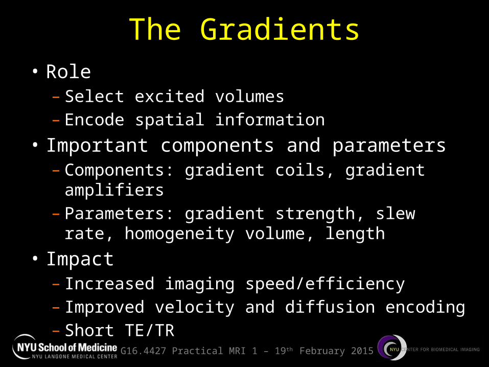
Qualitative Description



Spin Echo and Gradient EchoWhen the prephasing gradient is applied the spins accumulate phase (differently with location). After the 180° pulse, they will continue to accumulate phase under the influence of the readout gradient and will refocus at the echo time.• The echo is maximum when the area of the readout gradient is equal to the area of the prephasing lobe• If the echo coincide with the RF echo, then off-resonance effects are minimized

In the gradient echo sequence we don’t have the refocusing pulse, so the prephasing lobe has the opposite polarity. What does this tell you about an important difference with spin-echo?Bernstein et al. (2004) Handbook of MRI Pulse Sequences


Readout Gradient DesignThe duration of data acquisition Tacq is determined by the receiver bandwidth ±BW and the number of k-space data points along the readout direction nx ( ∆t = sampling time)

The amplitude of the readout gradient plateau can be derived from the FOV along the readout direction Lx

Which for a constant readout gradient has a simple k-space expression

The higher the readout gradient amplitude, the smaller the FOV that can be achieved. This can be done also by reducing the receiver bandwidth: why the former approach is preferable?


Prephasing Gradient Design

There is no requirement on the amplitude of the prephasing gradient as long as the area satisfies the equations above.• max amplitude can be used to minimize echo time (e.g. in angiography)• longer duration and smaller amplitude reduce the effect of eddy currents

In gradient echo with partial-echo (readout is not applied symmetrically with respect to techo) acquisition, if nx,f points are acquired prior to the center of the echo (nx,f ≤ nx/2), before using the above equation, techo must be calculated as:

In a full-echo acquisition (techo = Tacq/2), at techo the readout gradient area equals the prephasing gradient area (techo defines the point when the center of k-space is sampled):

Spin-echo

Gradient-echo


See you next week!

Documents

G16.4427 Practical MRI 1 – 19 th February 2015 G16.4427 Practical MRI 1 Gradients