g x v x h x;t v t dt f x (1) 1 t For a function Lp Lpotts/cms/cms13/slides/Capobianco... · We recall that,since ﬁ = ﬂ = 1 2, the n-th orthonormal Tchebychev polynomial of the

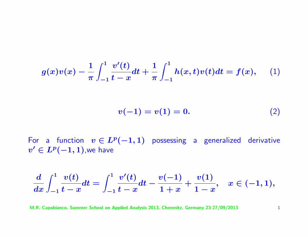
g(x)v(x) − 1

π

∫ 1

−1

v′(t)

t − xdt +

1

π

∫ 1

−1h(x, t)v(t)dt = f(x), (1)

v(−1) = v(1) = 0. (2)

For a function v ∈ Lp(−1, 1) possessing a generalized derivativev′ ∈ Lp(−1, 1),we have

d

dx

∫ 1

−1

v(t)

t − xdt =

∫ 1

−1

v′(t)

t − xdt − v(−1)

1 + x+

v(1)

1 − x, x ∈ (−1, 1),

M.R. Capobianco, Summer School on Applied Analysis 2013, Chemnitz, Germany 23-27/09/2013 1

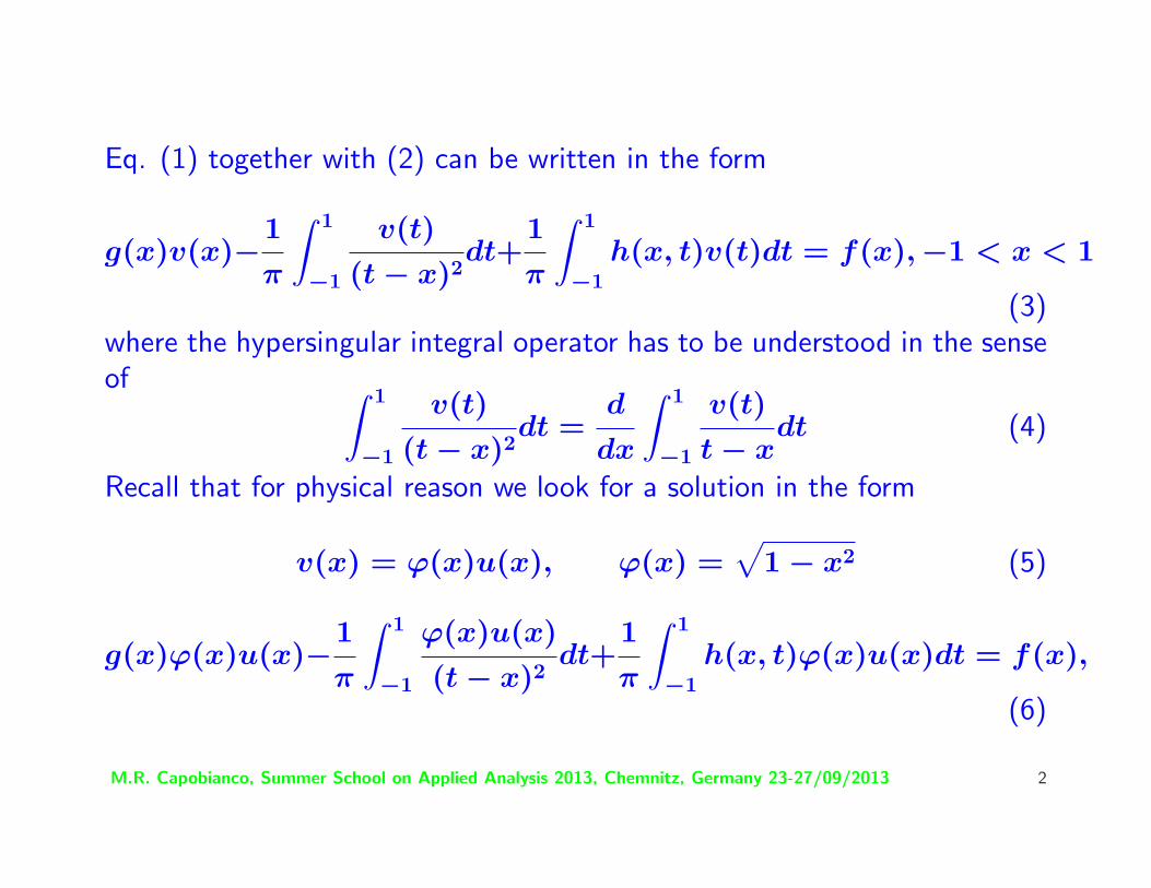
Eq. (1) together with (2) can be written in the form

g(x)v(x)−1

π

∫ 1

−1

v(t)

(t − x)2dt+

1

π

∫ 1

−1h(x, t)v(t)dt = f(x), −1 < x < 1

(3)where the hypersingular integral operator has to be understood in the senseof ∫ 1

−1

v(t)

(t − x)2dt =

d

dx

∫ 1

−1

v(t)

t − xdt (4)

Recall that for physical reason we look for a solution in the form

v(x) = ϕ(x)u(x), ϕ(x) =√

1 − x2 (5)

g(x)ϕ(x)u(x)−1

π

∫ 1

−1

ϕ(x)u(x)

(t − x)2dt+

1

π

∫ 1

−1h(x, t)ϕ(x)u(x)dt = f(x),

(6)


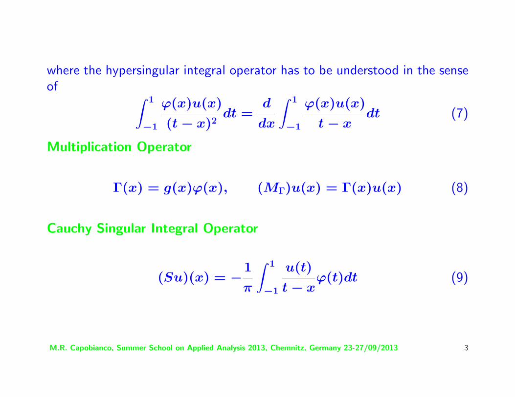
where the hypersingular integral operator has to be understood in the senseof ∫ 1

−1

ϕ(x)u(x)

(t − x)2dt =

d

dx

∫ 1

−1

ϕ(x)u(x)

t − xdt (7)

Multiplication Operator

Γ(x) = g(x)ϕ(x), (MΓ)u(x) = Γ(x)u(x) (8)

Cauchy Singular Integral Operator

(Su)(x) = −1

π

∫ 1

−1

u(t)

t − xϕ(t)dt (9)


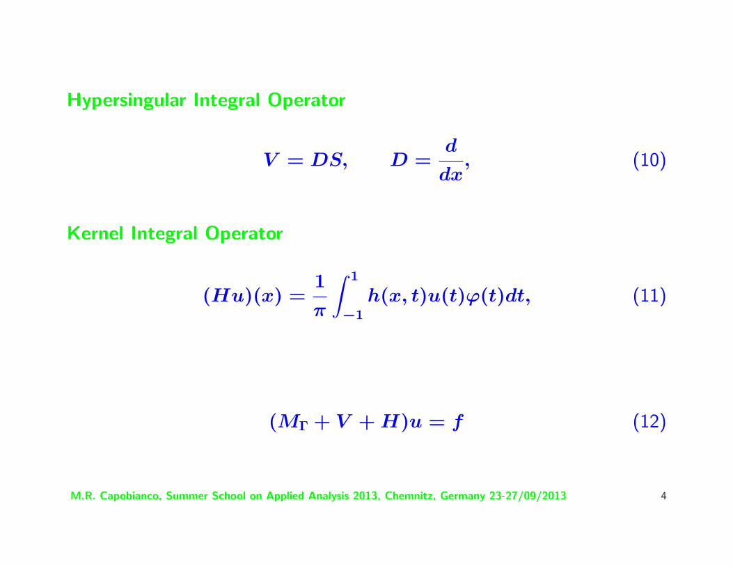
Hypersingular Integral Operator

V = DS, D =d

dx, (10)

Kernel Integral Operator

(Hu)(x) =1

π

∫ 1

−1h(x, t)u(t)ϕ(t)dt, (11)

(MΓ + V + H)u = f (12)


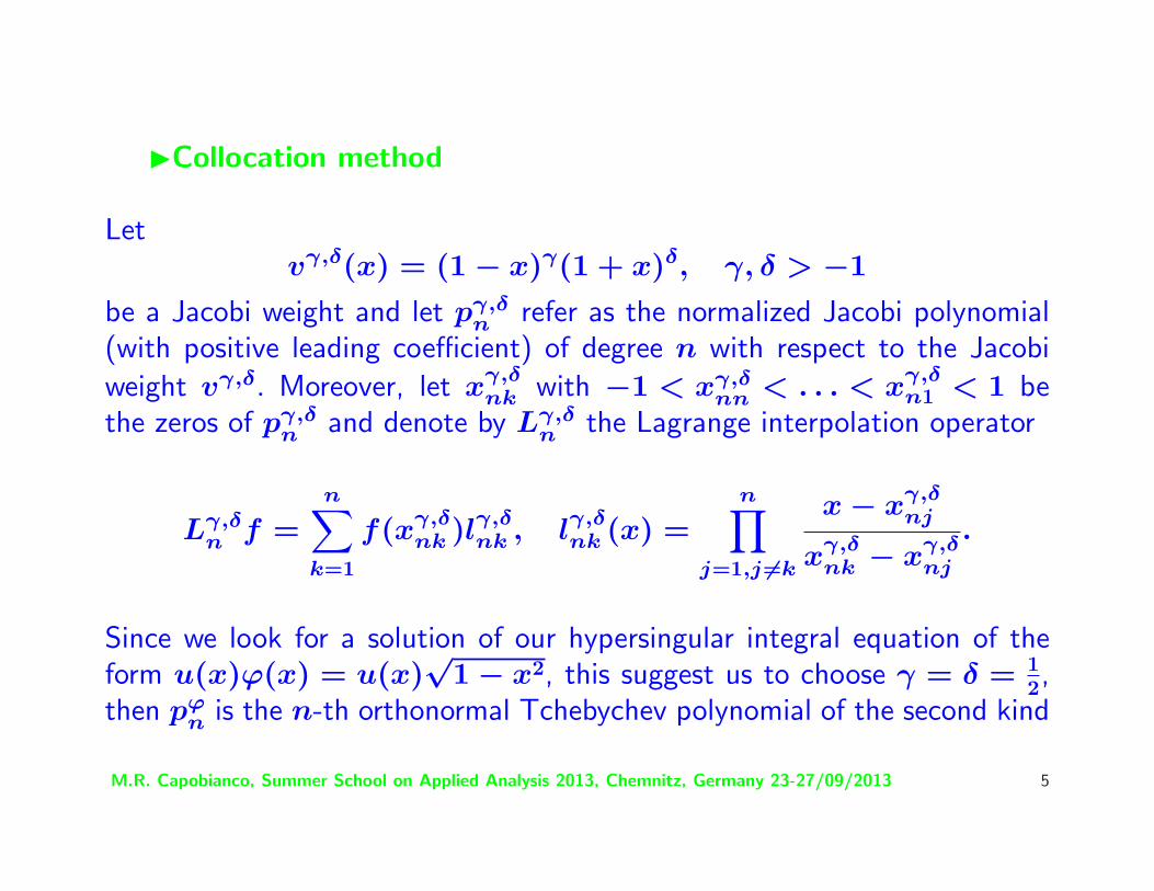
ICollocation method

Letvγ,δ(x) = (1 − x)γ(1 + x)δ, γ, δ > −1

be a Jacobi weight and let pγ,δn refer as the normalized Jacobi polynomial

(with positive leading coefficient) of degree n with respect to the Jacobi

weight vγ,δ. Moreover, let xγ,δnk with −1 < xγ,δ

nn < . . . < xγ,δn1 < 1 be

the zeros of pγ,δn and denote by Lγ,δ

n the Lagrange interpolation operator

Lγ,δn f =

n∑

k=1

f(xγ,δnk )lγ,δ

nk , lγ,δnk (x) =

n∏

j=1,j 6=k

x − xγ,δnj

xγ,δnk − xγ,δ

nj

.

Since we look for a solution of our hypersingular integral equation of theform u(x)ϕ(x) = u(x)

√1 − x2, this suggest us to choose γ = δ = 1

2,then pϕ

n is the n-th orthonormal Tchebychev polynomial of the second kind


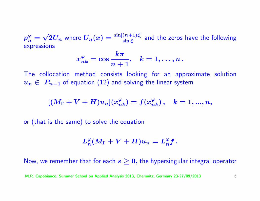
pϕn =

√2Un where Un(x) = sin[(n+1)ξ]

sin ξand the zeros have the following

expressions

xϕnk = cos

kπ

n + 1, k = 1, . . . , n .

The collocation method consists looking for an approximate solutionun ∈ Pn−1 of equation (12) and solving the linear system

[(MΓ + V + H)un](xϕnk) = f(xϕ

nk) , k = 1, ..., n,

or (that is the same) to solve the equation

Lϕn(MΓ + V + H)un = Lϕ

nf .

Now, we remember that for each s ≥ 0, the hypersingular integral operator


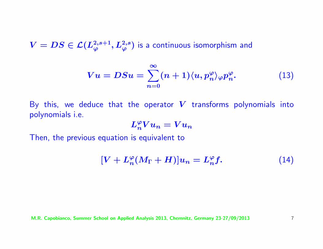
V = DS ∈ L(L2,s+1ϕ , L2,s

ϕ ) is a continuous isomorphism and

V u = DSu =∞∑

n=0

(n + 1)〈u, pϕn〉ϕpϕ

n. (13)

By this, we deduce that the operator V transforms polynomials intopolynomials i.e.

LϕnV un = V un

Then, the previous equation is equivalent to

[V + Lϕn(MΓ + H)]un = Lϕ

nf. (14)


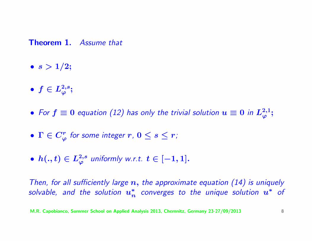
Theorem 1. Assume that

• s > 1/2;

• f ∈ L2,sϕ ;

• For f ≡ 0 equation (12) has only the trivial solution u ≡ 0 in L2,1ϕ ;

• Γ ∈ Crϕ for some integer r, 0 ≤ s ≤ r;

• h(., t) ∈ L2,sϕ uniformly w.r.t. t ∈ [−1, 1].

Then, for all sufficiently large n, the approximate equation (14) is uniquelysolvable, and the solution u∗

n converges to the unique solution u∗ of


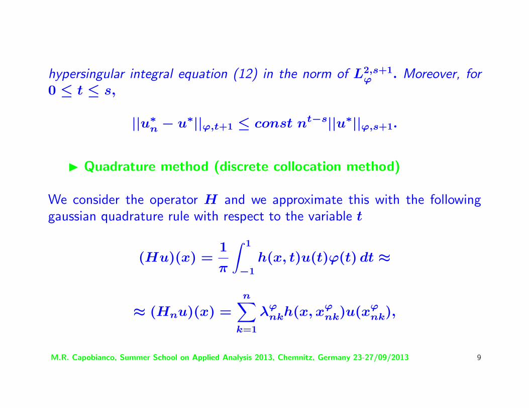
hypersingular integral equation (12) in the norm of L2,s+1ϕ . Moreover, for

0 ≤ t ≤ s,

||u∗n − u∗||ϕ,t+1 ≤ const nt−s||u∗||ϕ,s+1.

I Quadrature method (discrete collocation method)

We consider the operator H and we approximate this with the followinggaussian quadrature rule with respect to the variable t

(Hu)(x) =1

π

∫ 1

−1h(x, t)u(t)ϕ(t) dt ≈

≈ (Hnu)(x) =n∑

k=1

λϕnkh(x, xϕ

nk)u(xϕnk),


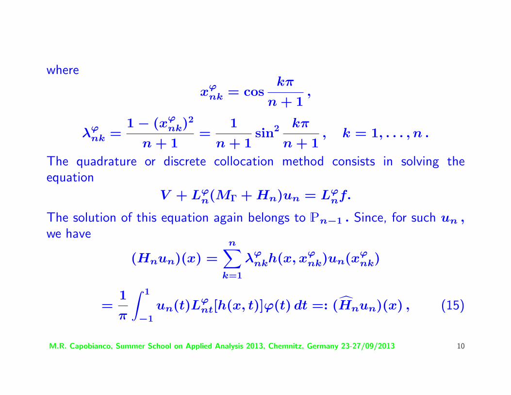
where

xϕnk = cos

kπ

n + 1,

λϕnk =

1 − (xϕnk)

2

n + 1=

1

n + 1sin2 kπ

n + 1, k = 1, . . . , n .

The quadrature or discrete collocation method consists in solving theequation

V + Lϕn(MΓ + Hn)un = Lϕ

nf.

The solution of this equation again belongs to Pn−1 . Since, for such un ,we have

(Hnun)(x) =n∑

k=1

λϕnkh(x, xϕ

nk)un(xϕnk)

=1

π

∫ 1

−1un(t)Lϕ

nt[h(x, t)]ϕ(t) dt =: (Hnun)(x) , (15)


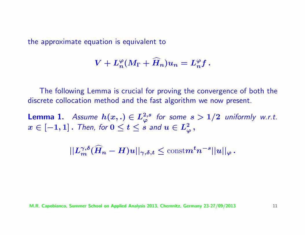
the approximate equation is equivalent to

V + Lϕn(MΓ + Hn)un = Lϕ

nf .

The following Lemma is crucial for proving the convergence of both thediscrete collocation method and the fast algorithm we now present.

Lemma 1. Assume h(x, .) ∈ L2,sϕ for some s > 1/2 uniformly w.r.t.

x ∈ [−1, 1] . Then, for 0 ≤ t ≤ s and u ∈ L2ϕ ,

||Lγ,δm (Hn − H)u||γ,δ,t ≤ constmtn−s||u||ϕ .


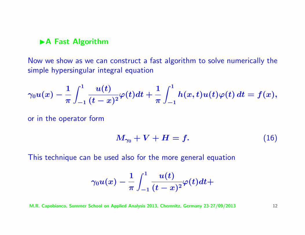
IA Fast Algorithm

Now we show as we can construct a fast algorithm to solve numerically thesimple hypersingular integral equation

γ0u(x) − 1

π

∫ 1

−1

u(t)

(t − x)2ϕ(t)dt +

1

π

∫ 1

−1h(x, t)u(t)ϕ(t) dt = f(x),

or in the operator form

Mγ0 + V + H = f. (16)

This technique can be used also for the more general equation

γ0u(x) − 1

π

∫ 1

−1

u(t)

(t − x)2ϕ(t)dt+


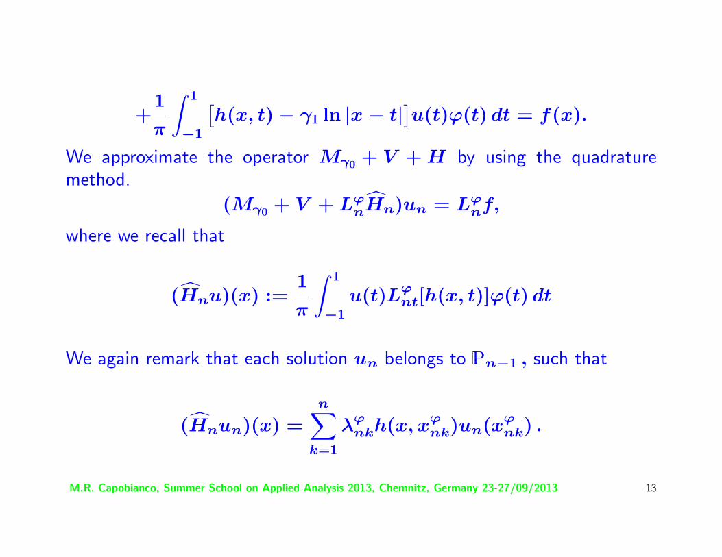
+1

π

∫ 1

−1

[h(x, t) − γ1 ln |x − t|]u(t)ϕ(t) dt = f(x).

We approximate the operator Mγ0 + V + H by using the quadraturemethod.

(Mγ0 + V + LϕnHn)un = Lϕ

nf,

where we recall that

(Hnu)(x) :=1

π

∫ 1

−1u(t)Lϕ

nt[h(x, t)]ϕ(t) dt

We again remark that each solution un belongs to Pn−1 , such that

(Hnun)(x) =n∑

k=1

λϕnkh(x, xϕ

nk)un(xϕnk) .


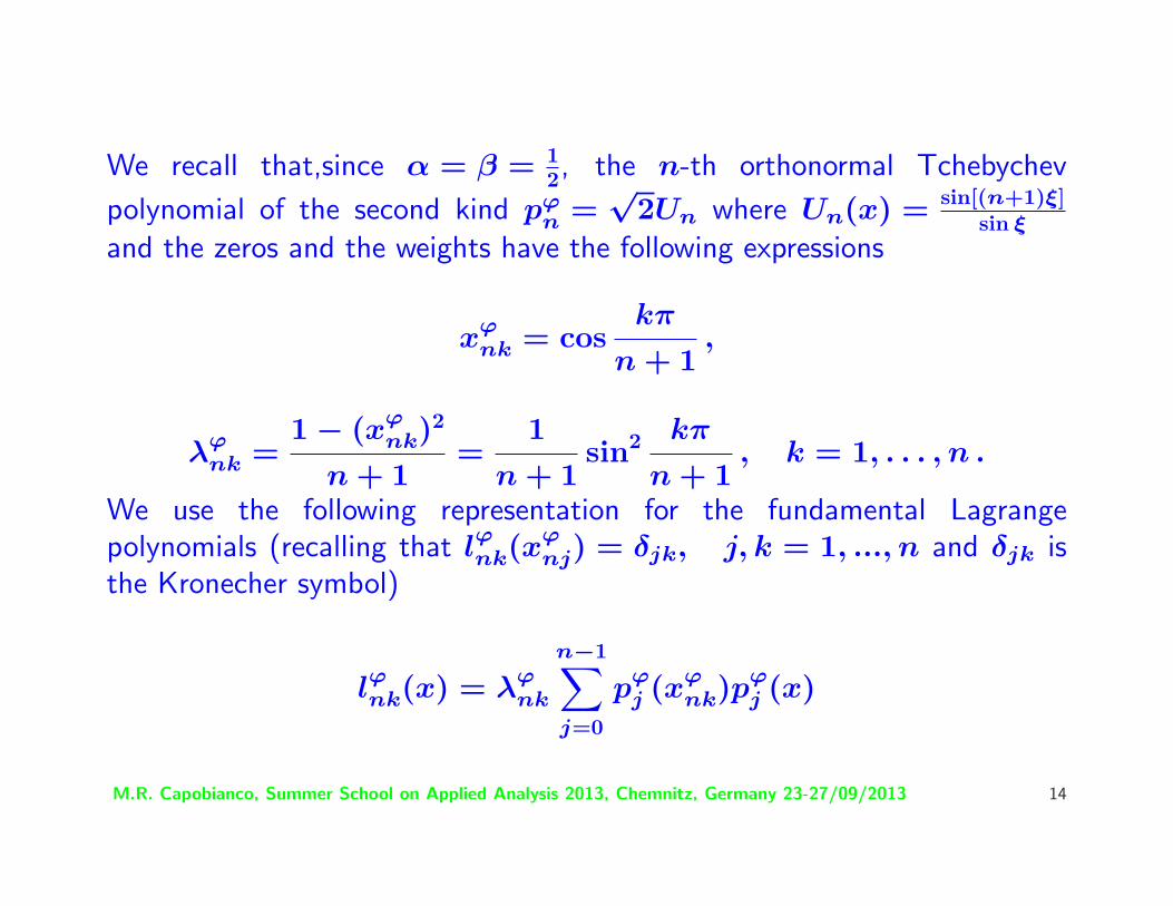
We recall that,since α = β = 12, the n-th orthonormal Tchebychev

polynomial of the second kind pϕn =

√2Un where Un(x) = sin[(n+1)ξ]

sin ξ

and the zeros and the weights have the following expressions

xϕnk = cos

kπ

n + 1,

λϕnk =

1 − (xϕnk)

2

n + 1=

1

n + 1sin2 kπ

n + 1, k = 1, . . . , n .

We use the following representation for the fundamental Lagrangepolynomials (recalling that lϕnk(x

ϕnj) = δjk, j, k = 1, ..., n and δjk is

the Kronecher symbol)

lϕnk(x) = λϕnk

n−1∑

j=0

pϕj (xϕ

nk)pϕj (x)


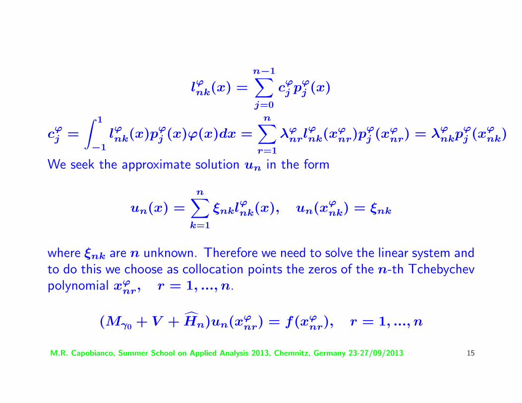
lϕnk(x) =n−1∑

j=0

cϕj pϕ

j (x)

cϕj =

∫ 1

−1lϕnk(x)pϕ

j (x)ϕ(x)dx =n∑

r=1

λϕnrl

ϕnk(x

ϕnr)p

ϕj (xϕ

nr) = λϕnkpϕ

j (xϕnk)

We seek the approximate solution un in the form

un(x) =n∑

k=1

ξnklϕnk(x), un(xϕnk) = ξnk

where ξnk are n unknown. Therefore we need to solve the linear system andto do this we choose as collocation points the zeros of the n-th Tchebychevpolynomial xϕ

nr, r = 1, ..., n.

(Mγ0 + V + Hn)un(xϕnr) = f(xϕ

nr), r = 1, ..., n


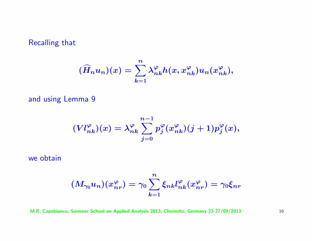
Recalling that

(Hnun)(x) =n∑

k=1

λϕnkh(x, xϕ

nk)un(xϕnk),

and using Lemma 9

(V lϕnk)(x) = λϕnk

n−1∑

j=0

pϕj (xϕ

nk)(j + 1)pϕj (x),

we obtain

(Mγ0un)(xϕnr) = γ0

n∑

k=1

ξnklϕnk(xϕnr) = γ0ξnr


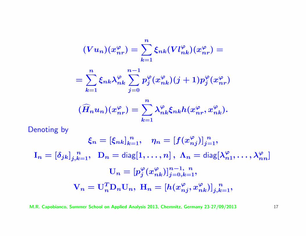
(V un)(xϕnr) =

n∑

k=1

ξnk(V lϕnk)(xϕnr) =

=n∑

k=1

ξnkλϕnk

n−1∑

j=0

pϕj (xϕ

nk)(j + 1)pϕj (xϕ

nr)

(Hnun)(xϕnr) =

n∑

k=1

λϕnkξnkh(xϕ

nr, xϕnk).

Denoting by

ξn = [ξnk] nk=1, ηn = [f(xϕ

nj)]n

j=1,

In = [δjk] nj,k=1, Dn = diag[1, . . . , n] , Λn = diag[λϕ

n1, . . . , λϕnn]

Un = [pϕj (xϕ

nk)]n−1, nj=0,k=1,

Vn = UTnDnUn, Hn = [h(xϕ

nj, xϕnk)]

nj,k=1,


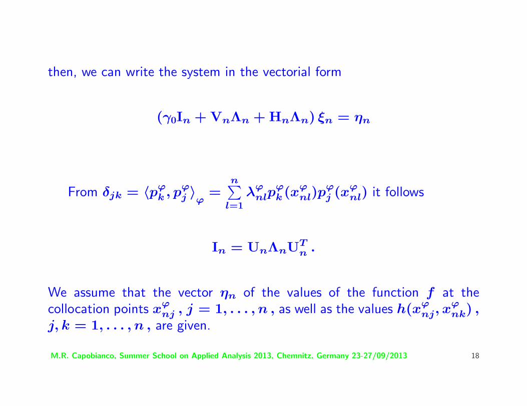
then, we can write the system in the vectorial form

(γ0In + VnΛn + HnΛn) ξn = ηn

From δjk = 〈pϕk , pϕ

j 〉ϕ

=n∑

l=1λϕ

nlpϕk(xϕ

nl)pϕj (xϕ

nl) it follows

In = UnΛnUTn .

We assume that the vector ηn of the values of the function f at thecollocation points xϕ

nj , j = 1, . . . , n , as well as the values h(xϕnj, xϕ

nk) ,j, k = 1, . . . , n , are given.


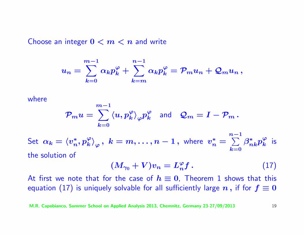
Choose an integer 0 < m < n and write

un =m−1∑

k=0

αkpϕk +

n−1∑

k=m

αkpϕk = Pmun + Qmun ,

where

Pmu =m−1∑

k=0

〈u, pϕk〉ϕpϕ

k and Qm = I − Pm .

Set αk = 〈v∗n, pϕ

k〉ϕ

, k = m, . . . , n − 1 , where v∗n =

n−1∑k=0

β∗nkpϕ

k is

the solution of

(Mγ0 + V )vn = Lϕnf . (17)

At first we note that for the case of h ≡ 0, Theorem 1 shows that thisequation (17) is uniquely solvable for all sufficiently large n , if for f ≡ 0


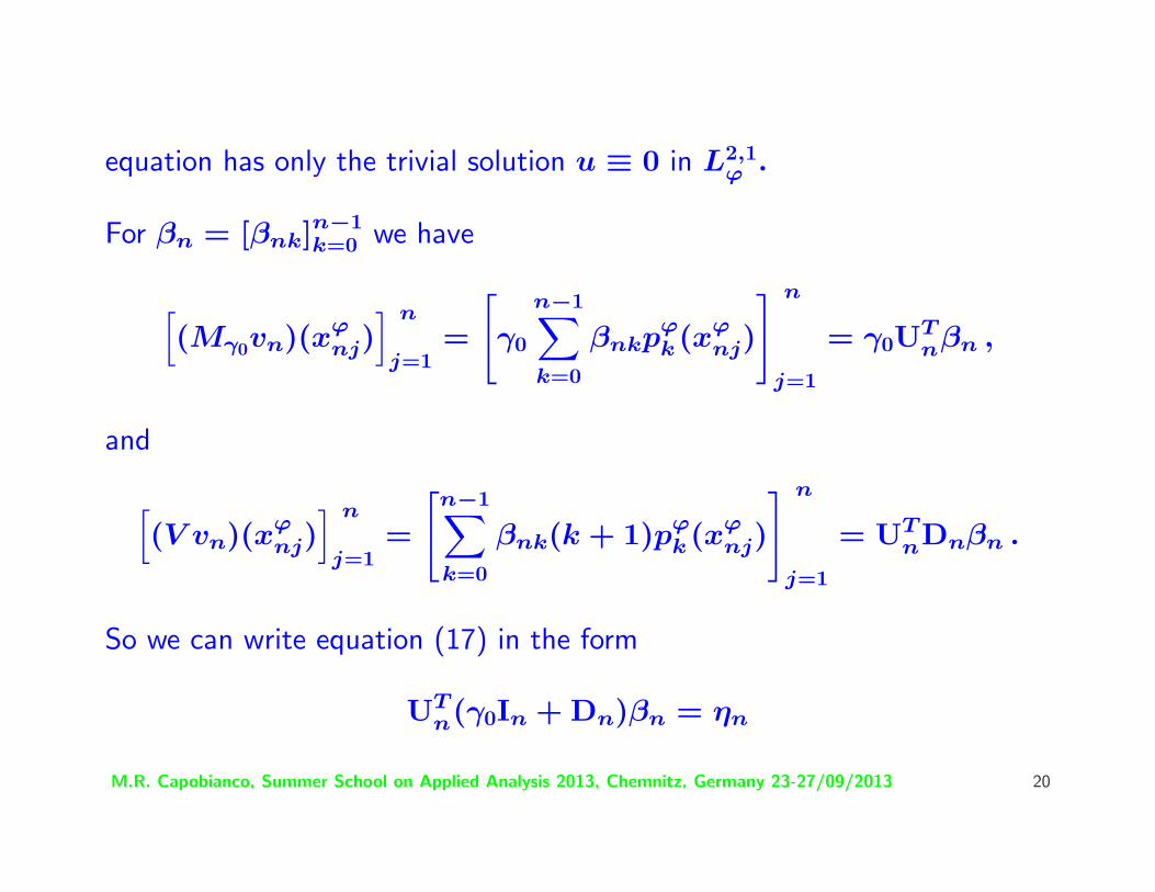
equation has only the trivial solution u ≡ 0 in L2,1ϕ .

For βn = [βnk]n−1k=0 we have

[(Mγ0vn)(xϕ

nj)] n

j=1=

[γ0

n−1∑

k=0

βnkpϕk(xϕ

nj)

] n

j=1

= γ0UTnβn ,

and

[(V vn)(xϕ

nj)] n

j=1=

[n−1∑

k=0

βnk(k + 1)pϕk(xϕ

nj)

] n

j=1

= UTnDnβn .

So we can write equation (17) in the form

UTn(γ0In + Dn)βn = ηn


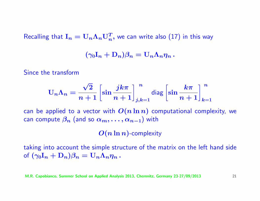
Recalling that In = UnΛnUTn, we can write also (17) in this way

(γ0In + Dn)βn = UnΛnηn .

Since the transform

UnΛn =

√2

n + 1

[sin

jkπ

n + 1

] n

j,k=1diag

[sin

kπ

n + 1

] n

k=1

can be applied to a vector with O(n ln n) computational complexity, wecan compute βn (and so αm, . . . , αn−1) with

O(n ln n)-complexity

taking into account the simple structure of the matrix on the left hand sideof (γ0In + Dn)βn = UnΛnηn .


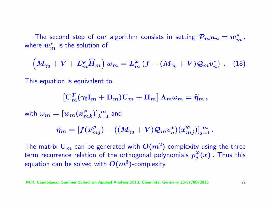
The second step of our algorithm consists in setting Pmun = w∗m ,

where w∗m is the solution of

(Mγ0 + V + Lϕ

mHm

)wm = Lϕ

m

(f − (Mγ0 + V )Qmv∗

n

). (18)

This equation is equivalent to

[UT

m(γ0Im + Dm)Um + Hm

]Λmωm = ηm ,

with ωm = [wm(xϕmk)]

mk=1 and

ηm = [f(xϕmj) − ((Mγ0 + V )Qmv∗

n)(xϕmj)]

mj=1 .

The matrix Um can be generated with O(m2)-complexity using the threeterm recurrence relation of the orthogonal polynomials pϕ

j (x) . Thus this

equation can be solved with O(m3)-complexity.


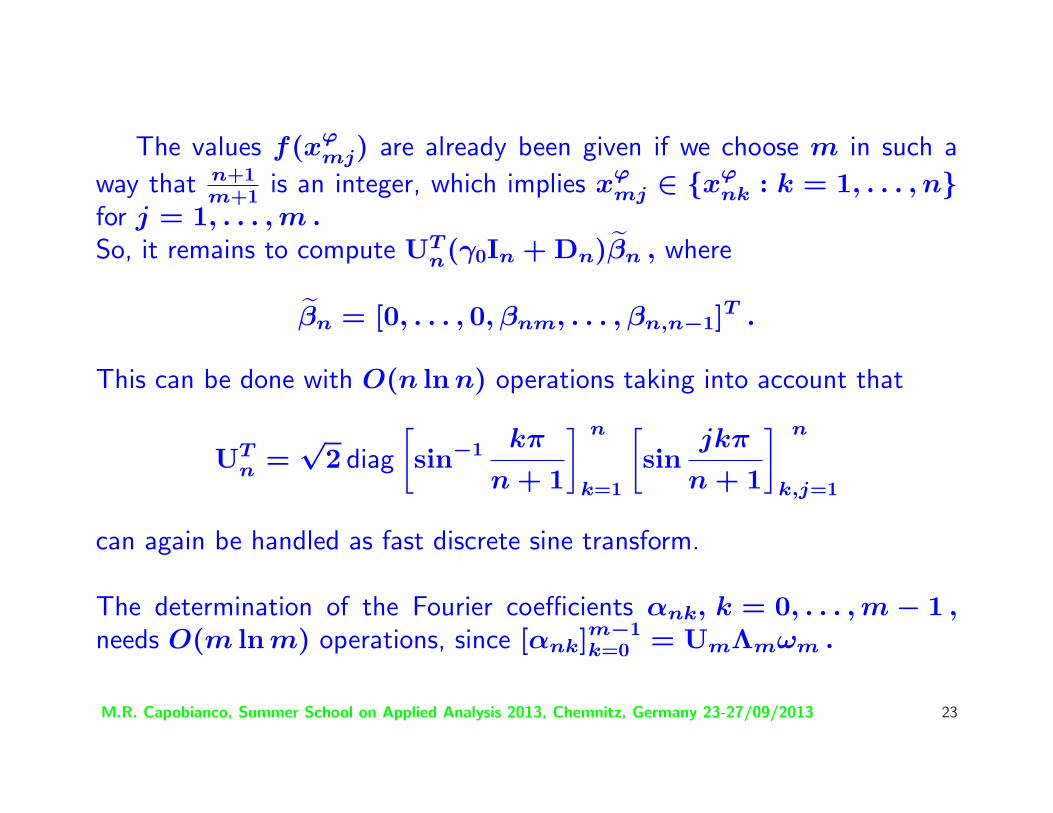
The values f(xϕmj) are already been given if we choose m in such a

way that n+1m+1 is an integer, which implies xϕ

mj ∈ {xϕnk : k = 1, . . . , n}

for j = 1, . . . , m .So, it remains to compute UT

n(γ0In + Dn)βn , where

βn = [0, . . . , 0, βnm, . . . , βn,n−1]T .

This can be done with O(n ln n) operations taking into account that

UTn =

√2 diag

[sin−1 kπ

n + 1

] n

k=1

[sin

jkπ

n + 1

] n

k,j=1

can again be handled as fast discrete sine transform.

The determination of the Fourier coefficients αnk, k = 0, . . . , m − 1 ,needs O(m ln m) operations, since [αnk]

m−1k=0 = UmΛmωm .


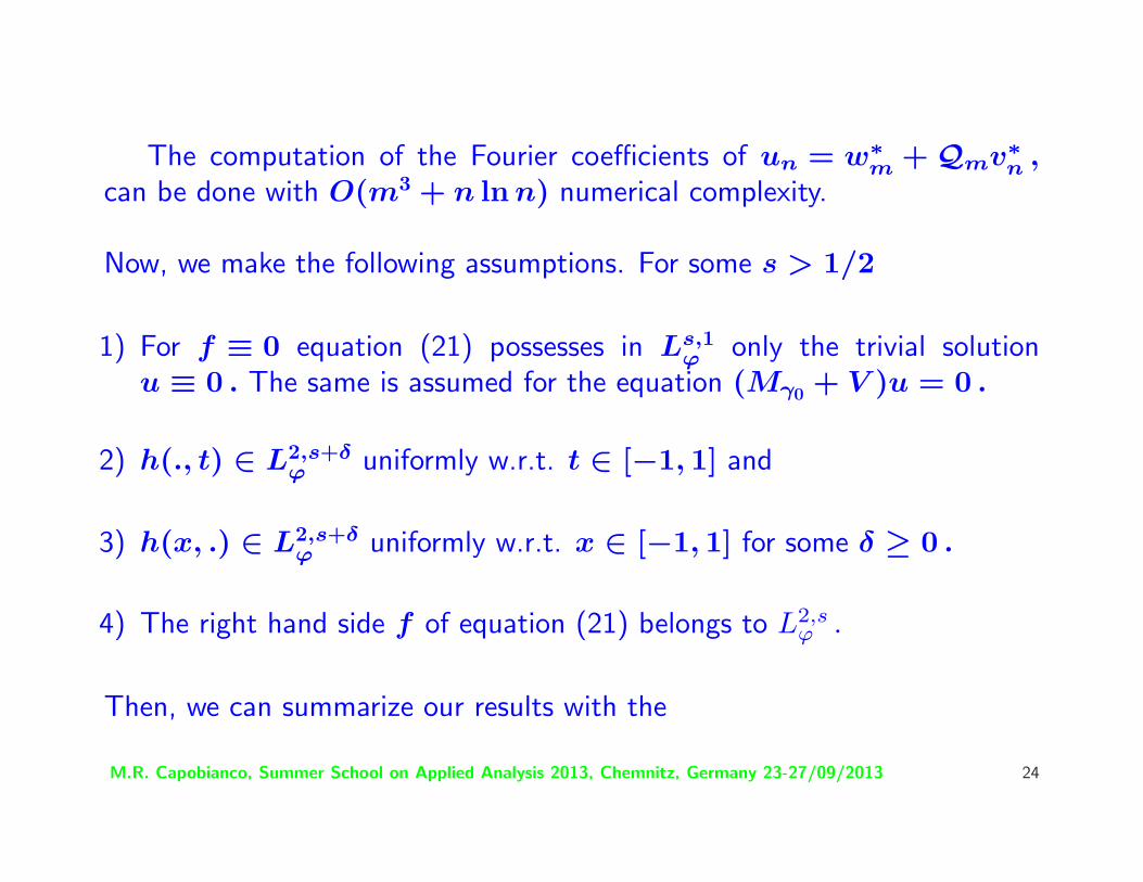
The computation of the Fourier coefficients of un = w∗m + Qmv∗

n ,can be done with O(m3 + n ln n) numerical complexity.

Now, we make the following assumptions. For some s > 1/2

1) For f ≡ 0 equation (21) possesses in Ls,1ϕ only the trivial solution

u ≡ 0 . The same is assumed for the equation (Mγ0 + V )u = 0 .

2) h(., t) ∈ L2,s+δϕ uniformly w.r.t. t ∈ [−1, 1] and

3) h(x, .) ∈ L2,s+δϕ uniformly w.r.t. x ∈ [−1, 1] for some δ ≥ 0 .

4) The right hand side f of equation (21) belongs to L2,sϕ .

Then, we can summarize our results with the


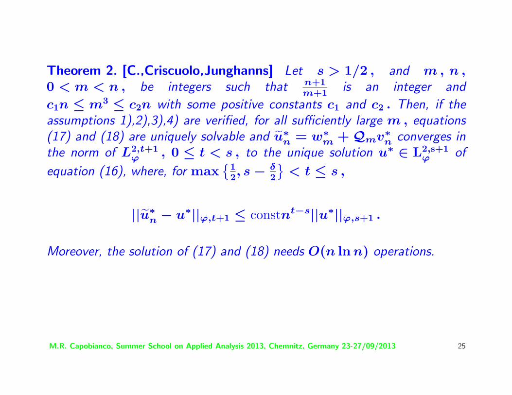
Theorem 2. [C.,Criscuolo,Junghanns] Let s > 1/2 , and m , n ,0 < m < n , be integers such that n+1

m+1 is an integer and

c1n ≤ m3 ≤ c2n with some positive constants c1 and c2 . Then, if theassumptions 1),2),3),4) are verified, for all sufficiently large m , equations(17) and (18) are uniquely solvable and u∗

n = w∗m + Qmv∗

n converges inthe norm of L2,t+1

ϕ , 0 ≤ t < s , to the unique solution u∗ ∈ L2,s+1ϕ of

equation (16), where, for max{1

2, s − δ2

}< t ≤ s ,

||u∗n − u∗||ϕ,t+1 ≤ constnt−s||u∗||ϕ,s+1 .

Moreover, the solution of (17) and (18) needs O(n ln n) operations.


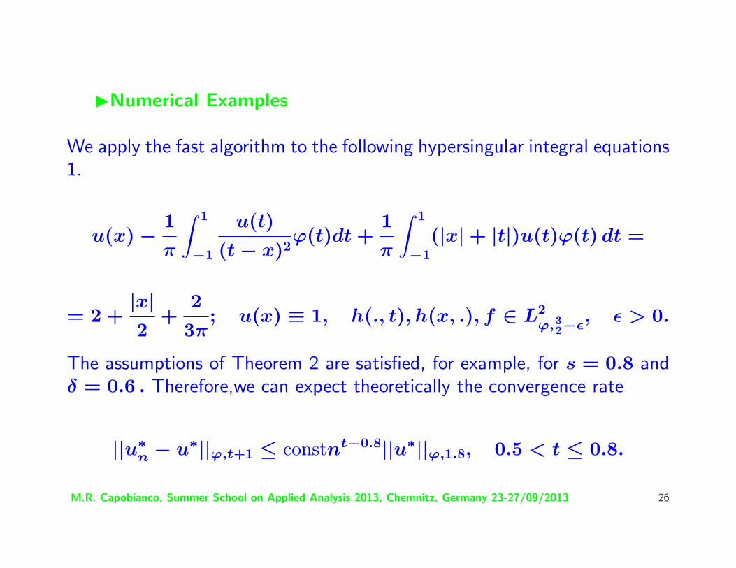
INumerical Examples

We apply the fast algorithm to the following hypersingular integral equations1.

u(x) − 1

π

∫ 1

−1

u(t)

(t − x)2ϕ(t)dt +

1

π

∫ 1

−1(|x| + |t|)u(t)ϕ(t) dt =

= 2 +|x|2

+2

3π; u(x) ≡ 1, h(., t), h(x, .), f ∈ L2

ϕ,32−ε, ε > 0.

The assumptions of Theorem 2 are satisfied, for example, for s = 0.8 andδ = 0.6 . Therefore,we can expect theoretically the convergence rate

||u∗n − u∗||ϕ,t+1 ≤ constnt−0.8||u∗||ϕ,1.8, 0.5 < t ≤ 0.8.


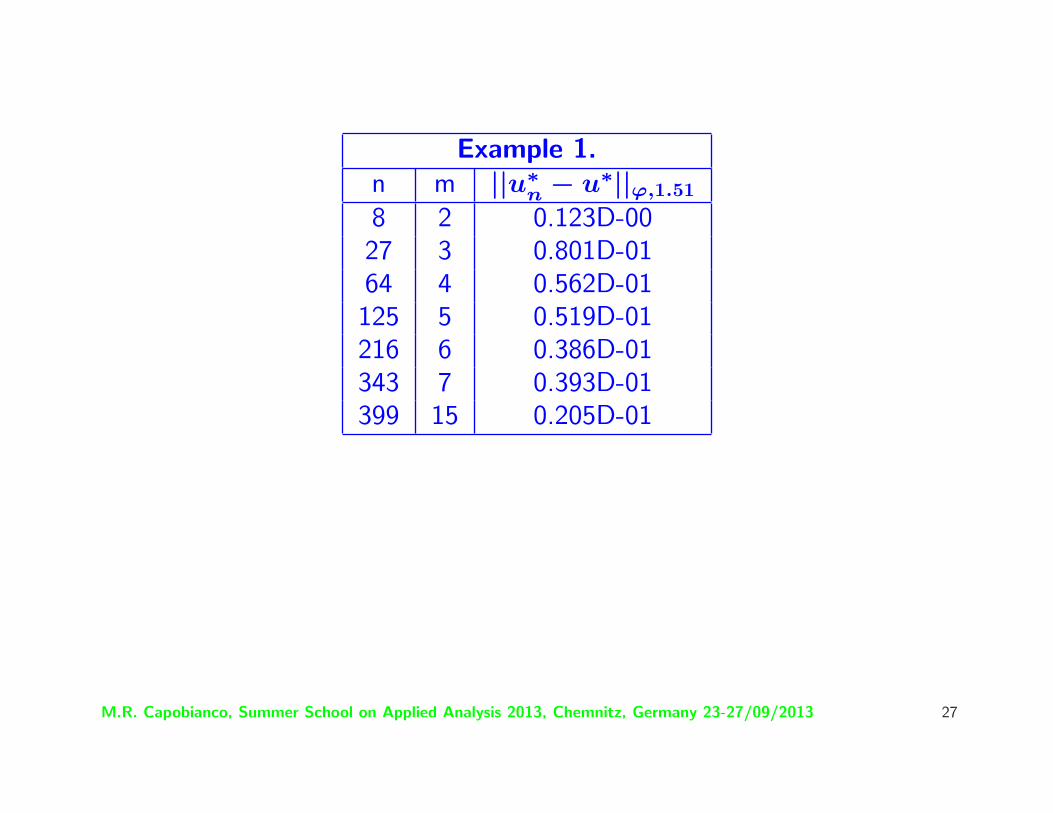
Example 1.n m ||u∗

n − u∗||ϕ,1.51

8 2 0.123D-0027 3 0.801D-0164 4 0.562D-01125 5 0.519D-01216 6 0.386D-01343 7 0.393D-01399 15 0.205D-01


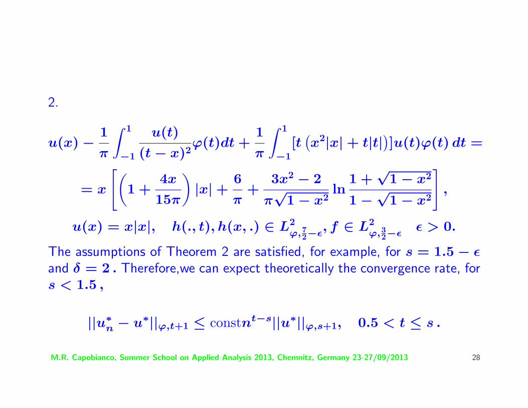
2.

u(x) − 1

π

∫ 1

−1

u(t)

(t − x)2ϕ(t)dt +

1

π

∫ 1

−1[t

(x2|x| + t|t|)]u(t)ϕ(t) dt =

= x

[(1 +

4x

15π

)|x| +

6

π+

3x2 − 2

π√

1 − x2ln

1 +√

1 − x2

1 − √1 − x2

],

u(x) = x|x|, h(., t), h(x, .) ∈ L2ϕ,72−ε

, f ∈ L2ϕ,32−ε

ε > 0.

The assumptions of Theorem 2 are satisfied, for example, for s = 1.5 − εand δ = 2 . Therefore,we can expect theoretically the convergence rate, fors < 1.5 ,

||u∗n − u∗||ϕ,t+1 ≤ constnt−s||u∗||ϕ,s+1, 0.5 < t ≤ s .


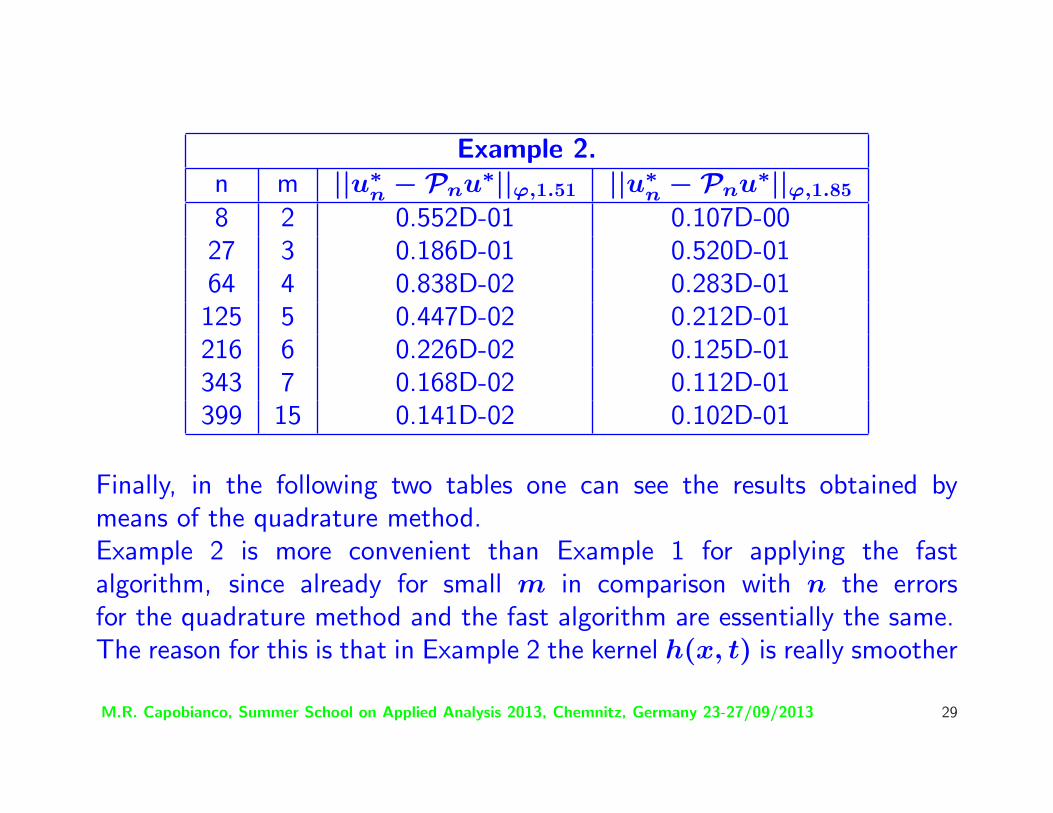
Example 2.n m ||u∗

n − Pnu∗||ϕ,1.51 ||u∗n − Pnu∗||ϕ,1.85

8 2 0.552D-01 0.107D-0027 3 0.186D-01 0.520D-0164 4 0.838D-02 0.283D-01125 5 0.447D-02 0.212D-01216 6 0.226D-02 0.125D-01343 7 0.168D-02 0.112D-01399 15 0.141D-02 0.102D-01

Finally, in the following two tables one can see the results obtained bymeans of the quadrature method.Example 2 is more convenient than Example 1 for applying the fastalgorithm, since already for small m in comparison with n the errorsfor the quadrature method and the fast algorithm are essentially the same.The reason for this is that in Example 2 the kernel h(x, t) is really smoother


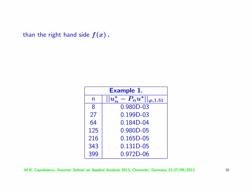
than the right hand side f(x) .

Example 1.n ||u∗

n − Pnu∗||ϕ,1.51

8 0.980D-0327 0.199D-0364 0.184D-04125 0.980D-05216 0.165D-05343 0.131D-05399 0.972D-06


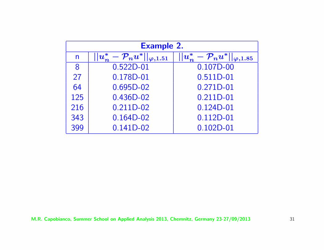
Example 2.n ||u∗

n − Pnu∗||ϕ,1.51 ||u∗n − Pnu∗||ϕ,1.85

8 0.522D-01 0.107D-0027 0.178D-01 0.511D-0164 0.695D-02 0.271D-01125 0.436D-02 0.211D-01216 0.211D-02 0.124D-01343 0.164D-02 0.112D-01399 0.141D-02 0.102D-01


Documents

g x v x h x;t v t dt f x (1) 1 t For a function Lp Lpotts/cms/cms13/slides/Capobianco... · We recall that,since ﬁ = ﬂ = 1 2, the n-th orthonormal Tchebychev polynomial of the