GROWTH AND STRUCTURAL CHANGE: TRENDS, PATTERNSAND POLICY OPTIONS

Bart Verspagen

Paper prepared for the conference on ‘Wachstums- und Innovationspolitik inDeutschland und Europa. Probleme, Reformoptionen und Strategien zu Beginn

des 21. Jahrhunderts’, Potsdam, 14 April 2000

First draft, April 2000

Eindhoven Center for Innovation Studies, EindhovenUniversity of Technology, PO Box 513, 5600 MB Eindhoven,

the Netherlands.

Maastricht Economic Research Institute on Innovation andTechnology, Maastricht University, PO Box 616, 6200 MD

Maastricht, the Netherlands.

1

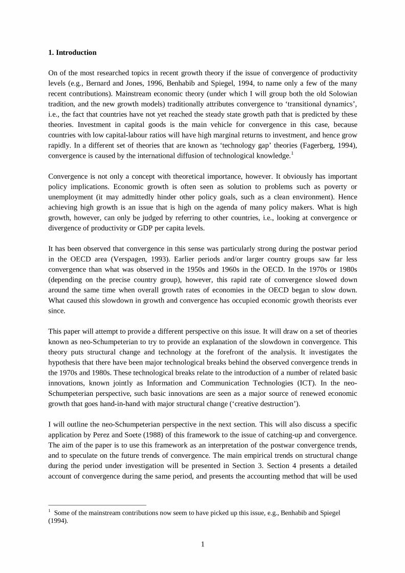
1. Introduction

On of the most researched topics in recent growth theory if the issue of convergence of productivitylevels (e.g., Bernard and Jones, 1996, Benhabib and Spiegel, 1994, to name only a few of the manyrecent contributions). Mainstream economic theory (under which I will group both the old Solowiantradition, and the new growth models) traditionally attributes convergence to ‘transitional dynamics’,i.e., the fact that countries have not yet reached the steady state growth path that is predicted by thesetheories. Investment in capital goods is the main vehicle for convergence in this case, becausecountries with low capital-labour ratios will have high marginal returns to investment, and hence growrapidly. In a different set of theories that are known as ‘technology gap’ theories (Fagerberg, 1994),convergence is caused by the international diffusion of technological knowledge.1

Convergence is not only a concept with theoretical importance, however. It obviously has importantpolicy implications. Economic growth is often seen as solution to problems such as poverty orunemployment (it may admittedly hinder other policy goals, such as a clean environment). Henceachieving high growth is an issue that is high on the agenda of many policy makers. What is highgrowth, however, can only be judged by referring to other countries, i.e., looking at convergence ordivergence of productivity or GDP per capita levels.

It has been observed that convergence in this sense was particularly strong during the postwar periodin the OECD area (Verspagen, 1993). Earlier periods and/or larger country groups saw far lessconvergence than what was observed in the 1950s and 1960s in the OECD. In the 1970s or 1980s(depending on the precise country group), however, this rapid rate of convergence slowed downaround the same time when overall growth rates of economies in the OECD began to slow down.What caused this slowdown in growth and convergence has occupied economic growth theorists eversince.

This paper will attempt to provide a different perspective on this issue. It will draw on a set of theoriesknown as neo-Schumpeterian to try to provide an explanation of the slowdown in convergence. Thistheory puts structural change and technology at the forefront of the analysis. It investigates thehypothesis that there have been major technological breaks behind the observed convergence trends inthe 1970s and 1980s. These technological breaks relate to the introduction of a number of related basicinnovations, known jointly as Information and Communication Technologies (ICT). In the neo-Schumpeterian perspective, such basic innovations are seen as a major source of renewed economicgrowth that goes hand-in-hand with major structural change (‘creative destruction’).

I will outline the neo-Schumpeterian perspective in the next section. This will also discuss a specificapplication by Perez and Soete (1988) of this framework to the issue of catching-up and convergence.The aim of the paper is to use this framework as an interpretation of the postwar convergence trends,and to speculate on the future trends of convergence. The main empirical trends on structural changeduring the period under investigation will be presented in Section 3. Section 4 presents a detailedaccount of convergence during the same period, and presents the accounting method that will be used

1 Some of the mainstream contributions now seem to have picked up this issue, e.g., Benhabib and Spiegel(1994).

2

to carry out the empirical analysis in Section 5. Section 6 concludes and tries to draw some (policy)lessons for the future.

2. Technology, Structural Change and Economic Growth: A Schumpeterian Perspective

The theoretical starting point for the analysis in this paper is Schumpeter’s theory about the economicimpact of technological revolutions (Schumpeter, 1939, see also Freeman and Soete, 1997). Thistheory is essentially a historical account of capitalism since the Industrial Revolution. It states thatmajor long-run fluctuations are caused by the clustering of so-called basic innovations during periodsof depression. Basic innovations are major technological breakthroughs, such as the steam engine, thedynamo, the internal combustion engine, or, more recently, the digital computer, the transistor, orgenetic engineering.

A major role in Schumpeter’s theory is played by the entrepreneur (an especially visionary businessman), who introduces the basic innovations in the economy, with the aim of making a profit (think ofBoulton and Watt, George and Robert Stephenson, or, more recently, Bill Gates, as the prototypeentrepreneurs). After its initial introduction, the basic innovations creates a bandwagon of imitations,each consisting of incrementally improved versions and enhancements of the basic design. It isthrough this bandwagon that the new technology diffuses through the economy, in a time period thatmay span decades. Because of the large opportunities for productivity and product qualityimprovement associated with the new technology, the economy grows at a rapid rate during thisdiffusion period.

In time, the technological opportunities for further improvement of the basic innovations wear off, andthe boom period comes to an end. A recession, and eventually depression, sets in, and the economyslowly gets ready for the next wave of basic innovations. The succession of boom, recession anddepression together forms a sequence of a long wave with 50-60 years periodicity. Schumpeterreferred to the work of the Russian economist Kondratiev, who had identified such long waves (mostlyin prices) in the 1920s, and after whom the phenomenon of long waves has been named afterwards.

There are many problems with Schumpeter’s theory, one of the obvious ones being that he did notexplain why basic innovations would cluster exactly during the depression periods of the long wave(Kuznets, 1940, was the first to bring out this point). A series of writings on the subject since the1970s (e.g., Mensch, 1979, Kleinknecht, 1981, Freeman, Clark et al., 1982, van Duijn, 1983) hasfurther developed and criticized this hypothesis. I will not be concerned with this specific debate here,but simply take the Schumpeterian argument about the impact of major technological breakthroughswithout strictly adhering to the notion of a long wave (with strict periodicity) as such. I will‘extrapolate’ (as many authors have done before me) the Schumpeterian argument by putting forwardthe hypothesis that modern Information and Communications Technologies (ICT) are a technologicalbreakthrough that have / will le(a)d to a period of prolonged economic growth in the OECD area (e.g.,Freeman and Soete, 1990, Freeman, 1994).

With this hypothesis, I will explore two issues. The first is the role of structural change in the processof economic growth driven by basic innovations. The second is the joint impact of structural changeand technological change on the level of disparity of labour productivity during the different phases ofthe growth process (long wave). The rest of this section will explore these issues from a theoretical

3

point of view, with the aim of formulating hypotheses about the medium-run tendencies for disparityof productivity levels in the largest OECD economies.

In Schumpeter’s theory, the introduction of basic innovations leads to a process of ‘creativedestruction’, in which sectors associated with the ‘old’ technologies decline, and new sectors emergeand grow. Freeman and Soete (1997) provide a historical overview of this process, discussing, amongother things, the role of ‘leading sectors’. Creative destruction, of course, is nothing else than a moreprosaic term for ‘structural change’, i.e., changes measured ultimately by variations in the shares of‘sectors’ in output or employment.

The overview in Freeman and Soete (1997) shows how technological change and creative destructionsince the First Industrial Revolution has mainly been taking place within the manufacturing sector,with transportation as the only services branch that was affected in a major way. Starting with textilesand clothing, the roughly two centuries since then have brought us new branches such as iron and steelmaking, chemicals, motor vehicles, machine tools and electronics. This has led authors such as Kaldor(1970) and Cornwall (1977) to formulate the hypothesis that the manufacturing sector bears specialimportance for economic growth in a broader sense.

In Kaldor (1966), the expansion of the manufacturing sector is seen as the driving force for economicgrowth. This expansion is essentially demand-driven, and is made possible by a shift of labour fromagriculture (where hidden unemployment is present) to manufacturing. Kaldor (1970) further developsthe factors behind strong growth in manufacturing. Here, he stresses the joint forces of demandincreases leading to increased productivity (via Verdoorn’s law), in turn leading to increased demand,thus setting in motion a process of ‘cumulative causation’. Dixon and Thirlwall (1975) haveformalized this argument in a regional setting.

The role of productivity increase in the manufacturing sector for macroeconomic growth is furtherstressed by Cornwall (1976) and Cornwall (1977). Cornwall develops Kaldor’s idea of manufacturingas a leading sector by explicitly referring to technological change in selected manufacturing sectors asa driving force for productivity improvement in a whole range of sectors, through technologicalinterdependence as well as input-output linkages between sectors. In this Kaldor-Cornwallperspective, manufacturing is thus seen as the prime sector leading to economic growth.

The technological revolution underlying the present upswing in economic growth, broadlycharacterized as ‘Information and Communication Technologies’ (ICT), is one that, although it wasoriginally based in manufacturing (microelectronics), is now primarily associated with the rise ofservices sectors such as business services (as an ICT using sector) and software development (as themain ICT generating sector) (Castells, 1996, Petit and Soete, 2000) This phenomenon may beinterpreted as the result of supply factors (the nature of basic innovations in ICT), as well as demandfactors. On the supply side, ‘information’ as the basic ingredient into ICT is by its nature an intangiblegood, and this naturally leads to a large importance of intangibles (services) alongside hardware(manufactured) in the changes associated with ICT.

On the demand side, the argument basically builds on Pasinetti's (1981) interpretation of economicgrowth. His theory stresses the role of demand in structural change. The basis for Pasinetti’s argumentis the Engel curve, which says that demand for any good eventually saturates at high levels of income.

4

In Pasinetti (1981), the emphasis is on the implications of this saturation for structural unemployment,but in his (1993) contribution, the implications for economic growth are analyzed more deeply as well.Saturation of demand for a good (declining income elasticities) leads to a slowdown of economicgrowth, just as the wearing-off of technological opportunities leads to a slowdown in Schumpeter’soriginal theory.

The interpretation is then that the demand for manufactured goods has reached a phase of decliningincome elasticity, thus leading to slower growth for countries specialized in the manufacturing sector,and providing opportunities for growth based on ICT (which, as was argued, has an important servicescontent). Such an argument supports the notion that ICT-based growth only takes off in full potentialafter developments on the service part of ICT (e.g., the internet) have gained crucial momentum.

Following this line of argument, Fagerberg and Verspagen (1999), put forward and tested thehypothesis that the Kaldor-Cornwall perspective on the importance of manufacturing was very specificto the time frame in which it was formulated (the 1960s and early 1970s). This period was, in the neo-Schumpeterian interpretation of Freeman and Soete (1997), the heyday of mass-production basedinnovation systems. This mode of production, initiated by basic innovations such as the assembly line,the motor car and plastics in the United States in the first half of the 20th century, is seen by these neo-Schumpeterian authors (e.g., Freeman and Soete, 1997) as the last ‘long wave’ based firmly inmanufacturing.

Fagerberg and Verspagen (1999) indeed found that the correlation between growth in manufacturingand overall growth was much weaker in the 1980s and 1990s than before, at least for the sample ofdeveloped (OECD) countries. In the (SouthEast Asian) NICs, manufacturing still plays a strong role,leading to the hypothesis that the manufacturing base of ICT has shifted to these countries. This isindeed a popular view (see also Castells, 1996) that corroborates with impressions one gets from tradestatistics.

What does this changing role of manufacturing in the light of technological revolutions and theirimpact on growth imply for comparative growth between the most advanced nations in OECD andEurope? I will attempt to tackle this issue by referring to the notion of technological catching-up. Thistheory is based on the ideas first raised by Gerschenkron (1962), and later formalized by Gomulka(1971). The hypothesis is that countries that are initially ‘backward’ in a technological sense have alarge potential to imitate knowledge from the more advanced countries. Because imitation is generallycheaper (but not costless) than innovation, this provides these ‘backward’ countries with a potentialfor high growth. One may say that this theory puts Schumpeter’s idea of bandwagons into aninternational perspective.

Whether or not the potential for such catching-up based economic growth is realized depends on howwell a country is able to assimilate knowledge from abroad. Such assimilation obviously requiresskills that depend, among other things, on human capital, the quality of the infrastructure, andinstitutions such as politics and banking. Abramovitz (1979) has used the term ‘social capability’ torefer to the set of factors that support assimilation of knowledge from abroad.

The importance that Abramovitz and others (Fagerberg, 1994) attach to social capability neatly linesup with the importance that authors such as Freeman (1986) and Perez (1983) attach to institutions in a

5

neo-Schumpeterian innovation of basic innovations and the long wave. These authors argue that eachnew set of basic innovations that form the starting point of the long wave create new institutionalrequirements. Most obviously, this relates to educational demand related to the new skills thattechnology requires, but one may also think of other factors. One example is the introduction ofstandardized time as a result of railroads, or the role of venture capital, universities and ‘culture’ insupporting major technological breakthroughs in ICT in Silicon Valley Saxenian (1994).

Combining the role of institutional factors in both the emergence of new growth related to basicinnovations, and catching-up based growth, Perez and Soete (1988) argue that catching-up basedgrowth is easier in some phases of the long wave than in others. Their main theoretical concept is thetechnology life cycle, which distinguishes four phases: introduction, early growth, late growth andmaturity. Perez and Soete argue that entry of countries in technological systems is easiest in either theintroduction phase, or the maturity phase. My interest here is mainly in entry during the introductionphase, so I will leave entry during the maturity phase unexplained.

In the introduction phase, there is little specific knowledge that is available or necessary for the newtechnological system. General (university) knowledge brings a country a long way to enter the newfield. Given that a country has a reasonably well-developed system of public knowledge generation,entry is thus relatively easy during the introduction phase of a new basic innovation. Entry becomesmuch more difficult in the growth phases, because then the technological system will have evolvedinto a state where tacit knowledge related to experience and learning-by-doing plays a much moreimportant role. Thus, one would expect that the foundations for catching-up based growth would belaid during the introduction phase of a new set of technologies, after which the ‘window ofopportunity’ closes again for a long period.

As will be argued below, the current situation in the world economy may be viewed as theintroduction phase of a new set of basic innovations, and hence ‘a window of opportunity’ for furtherconvergence to set in. Thus, I will try to apply the arguments by Perez and Soete to the currentsituation with regard to disparity of productivity levels, and try to draw conclusions on convergence inthe medium-run future.

However, Perez and Soete talk about opportunities, and they recognize that opportunities are notalways taken. Thus, although the potential for catching-up may be high during the introduction of anew technological system, one may also see that these opportunities are not taken. The ‘old leader’may be the country that implements the new technology earliest, and then further divergence may theresult rather than convergence.

What I will do in the remainder of this paper is interpret the recent history of convergence in the mostadvanced OECD countries in light of the two points made above. Summarizing, these two points are:

1. That structural change is a major part of technological revolutions and the economic growth theybring, and that the most recent technological revolution (ICT) has brought a declining role of themanufacturing sector in the most advanced OECD countries.2. That the rate of convergence of labour productivity (or catching-up based growth) is likely to differbetween periods, and that the ICT revolution may bring with it both divergence or convergence,

6

depending on how well other economies than the United States (the ‘old leader’) are able to adapt tothe technological breakthroughs.

3. Structural Change and Growth: Empirical Trends

This section will apply a database developed by researchers at the Groningen Growth andDevelopment Centre2 (GGDC) (see, e.g., Ark, 1996) to the issue of structural change and economicgrowth. The data used consist of value added data in constant prices and employment for six countries:Germany, France, Italy, United Kingdom, United States and Japan. Ten sectors are present in thedatabase, which will be introduced below. The GGDC database does not provide sectoral PurchasingPower Parities or similar variables that can be used to compare productivity and output levelsinternationally. I will therefore use OECD Purchasing Power Parities for the economy as a whole toconvert national currencies to US PPP $. Where the constant prices in the GGDC database do not referto 1990 (which is the base year for most countries), I use the US GDP price index to convert to 1990PPP $. Obviously, this approach introduces errors, but until a consistent dataset with sectoral PPPs isavailable, it is the best one can achieve.

0.0

0.1

0.2

0.3

0.4

0.5

0.6

0.7

0.8

0.9

1.0

1954 1959 1964 1969 1974 1979 1984 1989 1994

Manufacturing

Agriculture

Trade

Government

Community & Personal services

ConstructionTransport & Communication

Finance, Insurance & Real Estate

Figure 1. Employment shares in the 6 countries, 1954-1996

Figure 1 shows the share of labour resources devoted to each of the 10 sectors in the database. Theshares are weighted averages of the 6 countries. There are two primary sectors in the database:argiculture and mining. The manufacturing sector is considered as a total. The other sectors areconstruction; public utilities; wholesale and retail trade (trade); finance, insurance, real estate and

2 GGDC Sectoral Database, University of Groningen (Fourth Quarter 1999) (unpublished).

7

other business services; community and personal services; transport and communication, andgovernment services.

In the 1950s, the manufacturing sector was the largest of these 10 sectors, with approximately onequarter of total labour allocated to this sector (sectors are ranked according to their employment size in1954, larger sectors are lower in the figure). The two small sectors at the top of the figure are mining(lowest) and public utilities (highest). Table 1 gives more precise details about the relative decline andstagnation of the 10 sectors.

Table 1. Sectoral dynamics (employment share and labour productivity growth), 6 countriesaverage, 1965-1996

Share 1954 Share 1996 % increase share % Y growthManufacturing 0.25 0.18 -30.0 3.3Agriculture 0.21 0.04 -79.7 4.3Trade 0.15 0.20 34.8 2.2Government 0.13 0.16 28.6 0.4Community & Personal services 0.09 0.23 151.2 0.9Construction 0.06 0.07 6.9 0.9Transport & Communication 0.05 0.05 -0.3 3.1Finance, Insurance and Real Estate 0.03 0.06 121.6 1.3Mining 0.02 0.00 -76.9 3.7Utilities 0.01 0.01 -16.8 3.9

Until 1970, manufacturing slightly increases its share, but from then on, the sector declines in terms ofrelative employment. The share of agriculture falls sharply during the whole period. Together withmining, this is the sector that shows the largest percentual decrease of the labour share. Transport andcommunication (slightly) and utilities (and manufacturing) are the other sectors that see their share inemployment decline. The sectors with the strongest increase in employment are two services sectors:community and personal services, which grows from an already fairly large base in 1954, and finance,insurance and real estate, which is a much smaller sector (see also Petit and Soete, 2000).

Table 1 also gives the average annual compound growth rate of labour productivity in the sectors (6countries weighted average). Throughout the paper, labour productivity is defined as value added in1990 PPP $ per worker (per working hour would be a better indicators, but working hours are onlyavailable for a subset of the six countries). The results for labour productivity growth generally show atendency for productivity growth to be highest in sectors that produce tangible goods. Agricultureshows the highest growth rate, followed by the two energy related sectors (utilities, mining) andmanufacturing. The services sectors all show significantly lower productivity growth rates, especiallyso government, community and personal services and finance, insurance and real estate.

8

Manufacturing

-1.00

-0.50

0.00

0.50

1.00

DEU FRA GBR ITA JPN USA

1954

1996

Agriculture

-1.00

-0.50

0.00

0.50

1.00

DEU FRA GBR ITA JPN USA

1954

1996

Trade

-1.00

-0.50

0.00

0.50

1.00

DEU FRA GBR ITA JPN USA

1954

1996

Government

-1.00

-0.50

0.00

0.50

1.00

DEU FRA GBR ITA JPN USA

1954

1996

Community & Personal services

-1.00

-0.50

0.00

0.50

1.00

DEU FRA GBR ITA JPN USA

1954

1996

Construction

-1.00

-0.50

0.00

0.50

1.00

DEU FRA GBR ITA JPN USA

1954

1996

Transport & Communication

-1.00

-0.50

0.00

0.50

1.00

DEU FRA GBR ITA JPN USA

1954

1996

Finance, Insurance & Real Estate

-1.00

-0.50

0.00

0.50

1.00

DEU FRA GBR ITA JPN USA

1954

1996

Mining

-1.00

-0.50

0.00

0.50

1.00

DEU FRA GBR ITA JPN USA

1954

1996

Utilities

-1.00

-0.50

0.00

0.50

1.00

DEU FRA GBR ITA JPN USA

1954

1996

Figure 2. Specialization patterns

9

Taking these productivity growth rate at face value, and combining them with the increased labourshare of these sectors suggest the relevance of the analysis by Baumol (1967). This paper, that gaverise to the term ‘Baumol’s disease argues that a demand pattern that favours sectors with lowproductivity growth will eventually drive the economy to a state of low productivity growth. Keepingin mind the so-called productivity slowdown that hit the OECD countries during the 1970s, this seemsas a convincing explanation of events.

However, it is obvious that the services sectors with slow productivity growth in Table 1 are also thesectors that have large difficulties in measuring output (Ark, Monnikhof et al., 1999).This raises thesuspicion that the slow rates of productivity growth are seriously affected by measurement error.Certainly, anecdotal impressions one gets from, for example, the finance sector, would suggest thattechnological change and productivity growth play a much more important role that suggested byTable 1.

However, Baumol’s disease nor the issue of measurement of productivity and output in services arethe main topic of this paper. As explained in the introduction, the analysis here will instead look at therole of specific sectors in the process of convergence of labour productivity. In case the conclusionswould suggest that the above mentioned services industries are important for this process, this mightwell be related to an important extent to measurement issues.

To what extent do production structures really differ between the countries in our sample? Figure 2gives an answer to this question. The figure displays so-called revealed comparative advantage indicesfor each of the sectors. This index is constructed by first calculating the share of each country in asector’s total employment (across the 6 countries). This share is divided by the share of the country inoverall employment. Because the resulting indicator is not symmetric around its natural (weighted)mean, i.e., one, a correction is applied. The actual indicator used is calculated as (X-1)/(X+1), where Xis the ratio of the sectoral share and the overall share. This indicator lies between –1 and 1. A zerovalue corresponds to a neutral value, positive (negative) values point to (de)specialization in thesector.

Figure 2 gives the indicators for the years 1954 and 1996. While some of the specialization patternsobserved in 1954 persist in the period until 1996, there are also important reversals. In manufacturing,for example, such a reversal takes place in the UK (declining values of the indicator) and Japan(increasing values). Germany shows positive specialization in manufacturing over the whole period. Itmust be noted, however, that the values for all countries are rather close to zero, which indicates thatthe shares of manufacturing in labour do not differ too much between countries.

Agriculture shows a much more pronounced specialization pattern, with Italy and Japan as the twocountries specialized in this sector. The United Kingdom, the United States and, in 1996, Germanyshow strongly negative values. Mining is a sector that shows both strong specialization, and strongchanges in the specialization pattern over time. This is caused by important role of energy resources inthis sector.

In the services sector, trade and transport and communication show relatively even specializationpatterns. Community and personal services, and finance, insurance and real estate show larger

10

differences between countries. In the latter two sectors, the signs of the specialization patterns arerelatively stable.

How important are these differences for productivity growth? This question obviously has manytheoretical dimensions. A preliminary answer can be provided by a simple calculation, which isdisplayed in Table 2. The table displays a matrix, with countries in the rows and columns. The growthrates in the cells (percentages) were calculated as follows.

First, the level of labour productivity in each sector in each country was calculated for 1954 and 1996.Denote this by yij , with the subscripts i and j denoting a country and sector, respectively. From this,the annual average growth rate of labour productivity was calculated. This growth rate is indicated by

a hat above the variable. Then the share of each sector in total labour in a country was calculated (σij).

By definition, we have ∑=j

ijiji yy .σ Now define the alternative macroeconomic productivity level

∑=j

kjijik yy σ* , which is the hypothetical level of productivity using one country’s (k) structure, and

another country’s (i) productivity levels. This hypothetical level of productivity can be constructed for1954 and 1996, and the growth rate of this variable can be constructed. The value in row k, column i

of Table 2 is equal to .ˆˆ *iki yy − A positive number thus means that the country in the column would

‘benefit’ (in terms of productivity growth) from adopting the structure of the country in the row.

Table 2. The impact of structure on growthGrowthDEU FRA GBR ITA JPN USA

DEU 0.2 1.3 -0.1 -1.0 1.4FRA 0.1 1.1 0.0 -1.0 1.4GBR -0.8 -1.0 -0.3 -2.0 0.5ITA 0.1 -0.1 1.3 -1.1 1.0JPN 1.1 1.0 2.5 0.8 2.3

Structure

USA -1.7 -1.6 -0.5 -1.8 -2.8

Japan is the country that has the production structure that is most favourable to high productivitygrowth. This is indicated by the fact that all values in the column for Japan are negative. In otherwords, adopting any other production structure than its own would have a negative impact onproductivity growth in this country. The United States are the country with the ‘worst’ productionstructure, as indicated by all positive values in the column for this country. In Europe, the UnitedKingdom has a relatively ‘bad’ structure, while France, Germany and Italy show mixed results.

The finding that the United States and the United Kingdom have ‘bad’ economic structure is, ofcourse, related to their strong specialization in services, as shown in Figure 2. One has to keep inmind, however, the warning issued above about the measurement of productivity growth in services,which means that the results in Table 2 might be biased against these two countries.

11

4. Convergence of labour productivity levels

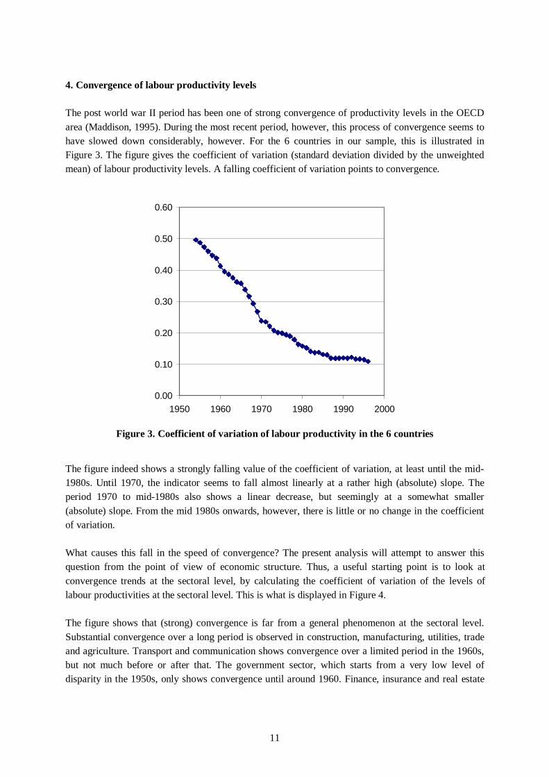
The post world war II period has been one of strong convergence of productivity levels in the OECDarea (Maddison, 1995). During the most recent period, however, this process of convergence seems tohave slowed down considerably, however. For the 6 countries in our sample, this is illustrated inFigure 3. The figure gives the coefficient of variation (standard deviation divided by the unweightedmean) of labour productivity levels. A falling coefficient of variation points to convergence.

0.00

0.10

0.20

0.30

0.40

0.50

0.60

1950 1960 1970 1980 1990 2000

Figure 3. Coefficient of variation of labour productivity in the 6 countries

The figure indeed shows a strongly falling value of the coefficient of variation, at least until the mid-1980s. Until 1970, the indicator seems to fall almost linearly at a rather high (absolute) slope. Theperiod 1970 to mid-1980s also shows a linear decrease, but seemingly at a somewhat smaller(absolute) slope. From the mid 1980s onwards, however, there is little or no change in the coefficientof variation.

What causes this fall in the speed of convergence? The present analysis will attempt to answer thisquestion from the point of view of economic structure. Thus, a useful starting point is to look atconvergence trends at the sectoral level, by calculating the coefficient of variation of the levels oflabour productivities at the sectoral level. This is what is displayed in Figure 4.

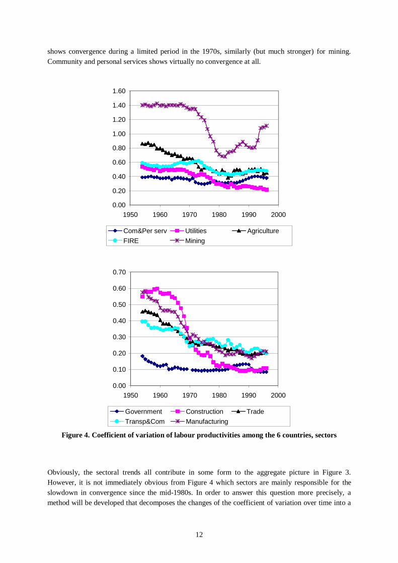
The figure shows that (strong) convergence is far from a general phenomenon at the sectoral level.Substantial convergence over a long period is observed in construction, manufacturing, utilities, tradeand agriculture. Transport and communication shows convergence over a limited period in the 1960s,but not much before or after that. The government sector, which starts from a very low level ofdisparity in the 1950s, only shows convergence until around 1960. Finance, insurance and real estate

12

shows convergence during a limited period in the 1970s, similarly (but much stronger) for mining.Community and personal services shows virtually no convergence at all.

0.00

0.20

0.40

0.60

0.80

1.00

1.20

1.40

1.60

1950 1960 1970 1980 1990 2000

Com&Per serv Utilities Agriculture

FIRE Mining

0.00

0.10

0.20

0.30

0.40

0.50

0.60

0.70

1950 1960 1970 1980 1990 2000

Government Construction Trade

Transp&Com Manufacturing

Figure 4. Coefficient of variation of labour productivities among the 6 countries, sectors

Obviously, the sectoral trends all contribute in some form to the aggregate picture in Figure 3.However, it is not immediately obvious from Figure 4 which sectors are mainly responsible for theslowdown in convergence since the mid-1980s. In order to answer this question more precisely, amethod will be developed that decomposes the changes of the coefficient of variation over time into a

13

contribution of the separate sectors. The method starts from the definition of the coefficient ofvariation (denoted by c):

,)(1

,1

, 22 ∑∑ −===i

ii

i myn

syn

mm

sc

where the subscript i indicates as before a country, and n is the number of countries (6).Differentiating c with respect to time gives (I use dots above variables to indicate a time derivative)

2m

smmsc

��

�

−= . In order to ‘translate’ to changes in productivity levels at the country level, one also

needs the following partial derivatives: .1

,ny

m

ns

my

y

s

i

i

i

=∂∂−

=∂∂

Substituting these into the expression

for c� gives

.∑

−

−=

i

ii

i

i cs

my

mn

y

y

yc

�

�

The first fraction under the summation sign is the proportionate growth rate of labour productivity in acountry. The second fraction is the country’s productivity level divided by the sum of productivitylevels in all countries. The terms between brackets give the deviation of the country’s productivitylevel relative to the mean, scaled by the standard deviation and the coefficient of variation. Hence, thechange of the coefficient of variation if a weighted sum of the productivity growth rates of theindividual countries. The sign of the weights depends on the magnitude of the country’s deviationfrom the mean productivity levels. Countries below the mean productivity level always have anegative weight (i.e., the more rapid they grow, the more rapid the coefficient of variation will fall).Countries with very high productivity levels have a positive weight, hence rapid growth in thesecountries increases disparity.3

The final step is to decompose the country growth rates of productivity. By definition, ∑=j

jj yy σ ,

hence aggregate productivity may change as a result of changes in the sectoral allocation of labour (σ)or sectoral productivity growth (y). Differentiating, one arrives at

+=⇒+= ∑∑

j

j

j

j

j

j

jjjjj y

y

q

q

y

yyyy

��

�

���

σσ

σσ )( , where q is production volume.

Substituting this into the above expression gives:

∑ ∑∑∑

−

−+

−

−=

j j j

jj

i

ii

j

jj

i

ii

q

qc

s

my

mn

y

y

y

q

qc

s

my

mn

yc .

σσ��

�

The first term on the right hand side is the effect related to (sectoral) productivity growth, which I willlabel as ‘technological progress’. The second term is related to changes in the allocation of labour tosectors, which I will label ‘structural change’. Within each of these terms, one can simply group allterms for a sector j, and sum them to obtain the change of the coefficient of variation that can beassociated with both technological progress and structural change in that sector. This can beformalized as follows:

3 Obviously, it is easy to derive formally the border line between negative and positive weights: .~ mcsyi +=

14

,,j

jj

ii

SCj

j

jj

ii

TPj

q

qFc

y

y

q

qFc

σσ�

�

�

� ∑∑ == with .

−

−= c

s

my

mn

yF ii

i

In this formula, the superscript TP denotes ‘technological progress’, the superscript SC denotesstructural change.

The derivation of the decomposition has been done in continuous time. Applying this to discrete datawould require a number of interaction terms, and this makes the formula quite complicated. One mayexpect that the impact of these interaction terms (in general, changes multiplied by changes) isrelatively small as compared to the non-interaction terms. Whether this is true or not can be assessedby approximating the real change of the coefficient of variation by the above formula (applied todiscrete data), and calculating the difference between the real change and the approximation. This iswhat was done, and in all cases the approximation was very close to the real value. Therefore, theanalysis here will not bother any further with the interaction terms, and present the results of thecalculations of the above formula applied to discrete data.

5. Empirical results and interpretation

One possibility for the slowdown in convergence would be that the macroeconomic scope forconvergence has become low as a result of convergence itself. In this case, the macroeconomicdifferences in productivity levels would be so small that further convergence was difficult to achieve.In terms of the decomposition method above, this would be reflected in the country-weights F. Figure5 presents the values of these weights over time.

The figure shows a remarkable pattern, evolving from an almost complete bipolar distribution to amuch more even one. In the 1950s, the United States has a high positive value of the weight, and allother countries a negative value. All these five countries with negative weights are grouped in a smallrange along the vertical axis. This means that, under the normal circumstance of positivemacroeconomic productivity growth, the United States alone are ‘responsible’ for any upwardpressure on the coefficient of variation during this period.

This situation changes slowly. The United States weight declines, and that for France, Italy andGermany increases. At the end of the period, these are the four countries with positive weights. Theweights for Japan and the United Kingdom also decline over time, and these two countries become theonly ones with negative weights at the end of the period.

The figure does not give any indication of what this implies for convergence. Undocumentedcalculations (available on request) show that the net impact of the changes in Figure 5 is very small.This was shown in an experiment in which the weights in the decomposition were fixed hypotheticallyat their 1960 value. In this case, the trend in the coefficient of variation was very similar to the oneactually observed. In 1996, the hypothetical coefficient of variation that results from the calculations is0.10, instead of the actually observed value of 0.11. The only period during which the differencebetween 1960 and actual weights is somewhat visible is the recession period 1989 - 1992, whichmostly affects the United Kingdom and Japan in Figure 5.

15

-0.30

-0.20

-0.10

0.00

0.10

0.20

0.30

0.40

0.50

0.60

1950 1960 1970 1980 1990 2000

Germany France UK Italy Japan USA

Figure 5. Country weights in the convergence decomposition

This result essentially shows that there is no convincing overall macroeconomic explanation behindthe convergence slowdown of the mid-1980s. The analysis will therefore turn to the sectoral level,using the decomposition technique introduced above. The technique gives calculations on the annualchange of the coefficient of variation. In order to rule out short-run fluctuations, the initial (annual)results were averaged over five year period, with the exception of the start and end of the overallperiod, where shorter time intervals were used. Figure 6 shows the overall results, summed over all 10sectors, but split up by the categories ‘structural change’ and ‘technological progress’.

The convergence slowdown is evident from the fact that the absolute value of the average yearlydecline of the coefficient of variation falls since the early 1970s. During 1985-1994, the changebecomes almost zero. Note that the last period in the graph overlaps with the previous period. Duringthis most recent period, the tendency for the coefficient of variation is to decline again (as is alsoevident in Figure 3).

Between the two categories ‘structural change’ and ‘technological progress’, the latter has the largestinfluence, except during the period 1956-1964, when the absolute value of the two factors iscomparable.4 However, the absolute value of both categories declines over time, so that one may saythat both factors contribute to the slowdown of convergence. For the most recent period, structuralchange even has a net diverging influence, as is shown by the positive values for this factor over the1990s.

4 It must be noted, however, that the short period (a year) over which the basic calculations were made, tends tohold down the value of the structural change component. Yearly changes in employment shares are small ascompared to yearly productivity growth rates. A similar effect, but in a different context, is found by Timmerand Szirmai (2000) and Fagerberg (2000).

16

Total

-0.025

-0.020

-0.015

-0.010

-0.005

0.000

0.005

19

56

-59

19

60

-64

19

65

-69

19

70

-74

19

75

-79

19

80

-84

19

85

-89

19

90

-94

19

94

-96

TP SC Total

Figure 6. The contribution of structural change and technological progress to the slowdown ofconvergence

Figure 7 presents the sectoral decomposition of the trends in Figure 6. Several conclusions emergefrom these graphs. First, with the exception of the small sectors mining and utilities, as well ascommunity and personal services, each of the sectors broadly shows a pattern in which the absolutevalue of the contribution to the convergence slow down becomes smaller over time, especially in the1970s. The most likely factor behind this general tendency is the overall slowdown of the rate oftechnological progress that may be associated with the slow maturing of the dominant technologicalsystem during this period.

Second, the manufacturing sector was by far the largest factor behind the strong convergence of the1960s and 1950s. The sudden decline of the manufacturing impulse for a falling coefficient ofvariation is also a large factor behind the slowdown of convergence in the 1970s and beyond. Thisresult is in general accordance with the Kaldor-Cornwall idea of the manufacturing sector as a drivingforce of economic growth during the period until the 1970s, and the findings by Fagerberg andVerspagen (1999) discussed above.

The explanation I offer for this result is the following. The 1950s and 1960s were a period in whichthe follower countries in the sample (all countries except the United States, see Figure 5) were able touse the manufacturing sector as a way of catching-up to the United States. This was possible becausethey had favourable conditions for entrance into the newly emerging technological system at thatstage. This new technological system consisted of mass-manufacturing, based on innovations thatwere introduced in the United States during the first half of the 20th century. Exogenous events such asthe second world war and the period of protectionism during the Great Depression of the 1930s‘deferred’ the start of this catch-up phase until the 1950s (Abramovitz and David, 1996).

17

Manufacturing

-0.010-0.009-0.008-0.007-0.006-0.005-0.004-0.003-0.002-0.0010.0000.0010.002

19

56

-59

19

60

-64

19

65

-69

19

70

-74

19

75

-79

19

80

-84

19

85

-89

19

90

-94

19

94

-96

SC

TP

Total

Agriculture

-0.010-0.009-0.008-0.007-0.006-0.005-0.004-0.003-0.002-0.0010.0000.0010.002

19

56

-59

19

60

-64

19

65

-69

19

70

-74

19

75

-79

19

80

-84

19

85

-89

19

90

-94

19

94

-96

SC

TP

Total

Trade

-0.010-0.009-0.008-0.007-0.006-0.005

-0.004-0.003-0.002-0.0010.0000.0010.002

19

56

-59

19

60

-64

19

65

-69

19

70

-74

19

75

-79

19

80

-84

19

85

-89

19

90

-94

19

94

-96

SC

TP

Total

Government

-0.010-0.009-0.008-0.007-0.006-0.005-0.004-0.003-0.002-0.0010.0000.0010.002

19

56

-59

19

60

-64

19

65

-69

19

70

-74

19

75

-79

19

80

-84

19

85

-89

19

90

-94

19

94

-96

SC

TP

Total

Community & personal services

-0.010-0.009-0.008-0.007-0.006-0.005-0.004-0.003-0.002-0.0010.0000.0010.002

19

56

-59

19

60

-64

19

65

-69

19

70

-74

19

75

-79

19

80

-84

19

85

-89

19

90

-94

19

94

-96

SC

TP

Total

Construction

-0.010-0.009-0.008-0.007-0.006-0.005-0.004-0.003-0.002-0.0010.0000.0010.002

19

56

-59

19

60

-64

19

65

-69

19

70

-74

19

75

-79

19

80

-84

19

85

-89

19

90

-94

19

94

-96

SC

TP

Total

Transport & communication

-0.010-0.009-0.008

-0.007-0.006-0.005-0.004-0.003-0.002-0.001

0.0000.0010.002

19

56

-59

19

60

-64

19

65

-69

19

70

-74

19

75

-79

19

80

-84

19

85

-89

19

90

-94

19

94

-96

SC

TP

Total

Finance, Insurance & real estate

-0.010-0.009-0.008-0.007-0.006-0.005-0.004-0.003-0.002-0.0010.0000.0010.002

19

56

-59

19

60

-64

19

65

-69

19

70

-74

19

75

-79

19

80

-84

19

85

-89

19

90

-94

19

94

-96

SC

TP

Total

Mining

-0.010-0.009-0.008-0.007-0.006-0.005-0.004-0.003-0.002-0.0010.000

0.0010.002

19

56

-59

19

60

-64

19

65

-69

19

70

-74

19

75

-79

19

80

-84

19

85

-89

19

90

-94

19

94

-96

SC

TP

Total

Utilities

-0.010-0.009-0.008-0.007

-0.006-0.005-0.004-0.003-0.002-0.001

0.0000.0010.002

19

56

-59

19

60

-64

19

65

-69

19

70

-74

19

75

-79

19

80

-84

19

85

-89

19

90

-94

19

94

-96

SC

TP

Total

Figure 7. Contributions to convergence slowdown, sectors

18

The favourable conditions that enabled the follower countries to enter the newly emergingtechnological system included institutional factors such as the Bretton-Woods system, the MarshallPlan, and the first phases of European economic and political integration. All of these factorscontributed to strong emphasis on economies of scale through increased international trade and strongexpansion of domestic demand (Nelson and Wright, 1992, Fagerberg, Guerrieri et al., 1999).

Having entered the new technological system at the crucial introduction phase (Perez and Soete,1988), a Kaldor-Cornwall type mechanism of manufacturing driven growth set in motion rapidcatching-up by these countries. However, because of the combined effect of demand saturation(Pasinetti, 1981) and the wearing-off of technological opportunities associated with the system ofmass-production, the scope for catching-up began to decline after a while. This is when the strongimpact of manufacturing on convergence, as well the contribution of other sectors to this process,begins to wear off in Figure 7.

A period of slow (or no) convergence arose since the early 1980s. In terms of the various contributionsto convergence in Figure 7, not much happened during this period. But below the surface of thestatistics, a new technological system started to emerge in the form of ICT. The mid-1990s,unfortunately the period where the data-availability stops, seem to have become the crucial phase forentry into the new technological system. If the countries in the sample are able to enter the new systemas successfully as they entered during the 1950s, one might expect a new phase of catching-up in thefuture. What are the signs of such an event that are already visible in the graphs?

One sector that is strongly associated with the new ICT system of production is the finance, insurance,real estate and other business services sector. It is remarkable that this sector is the one in Figure 7 thatshows the most steady behaviour over time. The overall contribution of this sector to convergence isnot extremely high, but given the size of the sector, still significant. Importantly, structural change is alarge component of this sector’s contribution. Still, there is somewhat of a decline in the convergencetendency of this sector in the 1990s. The main question is what will happen to this trend. The result forthe 1994-1996 period suggest that this effect is reversed, and that the sector gains a strong impulse forconvergence. If this tendency sets through, the sector might become a source of renewed convergencein the ICT system.

Trade, another sector highly affected by developments in ICT shows an opposite tendency during themost recent period. The same is true for manufacturing, which is still the sector that underlies a largepart of investment in ICT (hardware). Together, these three sectors may hold the key to futureconvergence or divergence.

6. Conclusions5

I have interpreted the convergence (of labour productivity) trend in a sample of the four largest EUcountries, the United States and Japan over the period 1955-1996 as the result of the ability of Europeand Japan to enter in the 1950s a set of technologies developed mainly in the United States known asthe ‘mass-production system’. This led to a process of convergence that was mainly driven by the

5 This section draws heavily on joint work with Jan Fagerberg and Paolo Guerrieri (Fagerberg, Guerrieri et al.(1999)). I alone am responsible, however, for the wording here.

19

manufacturing sector. When technological opportunities (in manufacturing) wore off, and demandsaturated, convergence slowed down, mainly since the mid-1980s.

In the mid-1990s, the world economy seems to witness the introduction phase of a new technologicalsystem, known as ICT. Although this system has a base in manufactured products (hardware), services(software as technology generating and mainly business services as technology using) plays a moreimportant role than ever. Whether or not convergence in the sample considered will pick up againdepends on whether or not the follower countries (the United States is widely seen as the leader ofboth the old and the new technological system) will be able to enter the new system adequately. If theyare not able to do so, the window of opportunity that is now open, may close because of cumulativelearning effects in the new technology (Perez and Soete, 1988).

Both national governments and the European Commission seem determined to stimulate the adoptionand generation of ICT in Europe, as was, for example, shown recently at the .com summit in Lisbon.Making ICT happen requires, however, an active and broad range of policies. Education is one ofthem, but here the issue seems more difficult than ‘to bring the internet into every classroom inEurope’. The process may also require the use of industrial policies in combination with R&Dpolicies, for example in order to maintain the traditional European stronghold of mobilecommunication. UMTS (the successor of GSM) may be a crucial initiative in this respect, andEuropean firms should be stimulated to take and maintain the technological lead in this field. Softwareseems to be a field where European performance is weak, however (Dalum, Freeman et al., 1999).Strategic thinking by the EU on how to turn recent developments such as the increased use of the opensource concept into a European advantage may be necessary.

The European Commission and national, regional and local governments may also play an importantand active role as suppliers of digital services. In almost all fields where citizens interact withgovernments, one may imagine networked applications. The broad development of these will bothincrease the demand for technically skilled (European) firms that can implement these services, andcreate value-added for users. One may imagine how a virtuous circle can be set in motion by suchgovernment procurement and government supply of digital services. Finally, supporting policies in theform of, for example, enabling venture capital to be raised more easily are important.

Together, these (and possibly other, the list here is far from exhaustive) initiatives present a break witha tradition of European integration aimed at economies of scale that was initiated in the 1950s. Thetearing down of trade barriers and the enlargement of the internal market has been a success story, andit has certainly added to the rapid growth and convergence that observed until the mid-1980s.However, in the new technological age, the concept of scale can no longer form the uniting principleof European policy and further integration. Economies of networks (in the broadest sense) may be amore appropriate device.

20

References

Abramovitz, M. A. (1979). Rapid Growth Potential and its Realisation : The Experience of CapitalistEconomies in the Postwar Period. Economic Growth and Resources, vol. 1 The major Issues,

Proceedings of the fifth World Congress of the International Economic Association. E. Malinvaud.London, Macmillan: 1-51.

Abramovitz, M. A. and P. A. David (1996). Convergence and deferred catch-up: productivityleadership and the waning of American exceptionalism. The Mosaic of Economic Growth. R.Landau, T. Taylor and G. Wright. Stanford, Stanford University Press: 21-62.

Ark, B. v. (1996). Sectoral Growth Accounting and Structural Change in Post-War Europe.Quantitative Aspects of Post-War European Economic Growth. B. van Ark and N. Crafts.Cambridge, Cambridge University Press: 84-164.

Ark, B. v., E. Monnikhof and N. Mulder (1999). “Productivity in Services: An InternationalComparative Perspective.” Canadian Journal of Economics 32: 471-499.

Baumol, W. (1967). “Macroeconomics of unbalanced growth.” American Economic Review 53: 941-973.

Benhabib, J. and M. M. Spiegel (1994). “The role of human capital in economic development:Evidence from aggregate cross-country data.” Journal of Monetary Economics 34: 143-173.

Bernard, A. B. and C. I. Jones (1996). “Comparing Apples to Oranges: Productivity Convergence andMeasurement Across Industries and Countries.” American Economic Review 86: 1216-1238.

Castells, M. (1996). The rise of the network society. Oxford, Blackwell.Cornwall, J. (1976). “Diffusion, Convergence and Kaldor's Laws.” Economic Journal 86: 307-314.Cornwall, J. (1977). Modern Capitalism. Its Growth and Transformation. London, Martin Robertson.Dalum, B., C. Freeman, R. Simonetti, et al. (1999). Europe and the Information and Communications

Technologies Revolution. The Economic Challenge to Europe. Adapting to Innovation BasedGrowth. J. Fagerberg, P. Guerrieri and B. Verspagen. Aldershot, Edward Elgar: 106-129.

Dixon, R. J. and A. P. Thirlwall (1975). “A Model of Regional Growth-Rate Differences on KaldorianLines.” Oxford Economic Papers 11: 201-214.

Fagerberg, J. (1994). “Technology and international differences in growth rates.” Journal of EconomicLiterature 32: 1147-1175.

Fagerberg, J. (2000). “Technological progress, structural change and productivity growth: acomparative study.” Structural Change and Economic Dynamics forthcoming.

Fagerberg, J., P. Guerrieri and B. Verspagen (1999). Europe - A Long View. The Economic Challenge

to Europe. Adapting to Innovation Based Growth. J. Fagerberg, P. Guerrieri and B. Verspagen.Aldershot, Edward Elgar: 1-20.

Freeman, C. (1986). Technology Policy and Economic Performance: Lessons from Japan. London,Pinter.

Freeman, C. (1994). Technological Revolutions and Catching-Up: ICT and the NICs. The Dynamics ofTrade, Technology and Growth. J. Fagerberg, B. Verspagen and N. Von Tunzelmann. Aldershot,Edward Elgar: 198-221.

Freeman, C., J. Clark and L. Soete (1982). Unemployment and Technical Innovation. London, Pinter.Freeman, C. and L. Soete (1990). “Fast Structural Change and Slow Productivity Change: Some

Paradoxes in the Economics of Information Technology.” Structural Change and EconomicDynamics 1: 225-242.

Freeman, C. and L. Soete (1997). The Economics of Industrial Innovation. 3rd Edition. London andWashington, Pinter.

21

Gerschenkron, A. (1962). Economic Backwardness in Historical Perspective. Cambridge MA,Harvard University Press.

Gomulka, S. (1971). Inventive Activity, Diffusion and the Stages of Economic Growth. Aarhus.Kaldor, N. (1966). Causes of the Slow Rate of Growth of the United Kingdom. Cambridge, Cambridge

University Press.Kaldor, N. (1970). “The Case for Regional Policies.” Scottish Journal of Political Economy XVII :

337-348.Kleinknecht, A. (1981). “Observations on the Schumpeterian Swarming of Innovations.” Futures 13.Kuznets, S. (1940). “Schumpeter's Business Cycles.” American Economic Review 30.Maddison, A. (1995). Monitoring the World Economy 1820-1992. Paris, OECD Development Centre.Mensch, G. (1979). Stalemate in Technology. Innovations Overcome Depression. Cambridge,

Ballinger.Nelson, R. R. and G. Wright (1992). “The rise and fall of American technological leadership: the

postwar era in an historical perspective.” Journal of Economic Literature 30: 1931-1964.Pasinetti, L. L. (1981). Structural Change and Economic Growth. A Theoretical Essay on the

Dynamics of the Wealth of Nations. Cambridge, Cambridge University Press.Perez, C. (1983). “Structural change and the assimilation of new technologies in the economic and

social systems.” Futures 15: 357-75.Perez, C. and L. Soete (1988). Catching Up in Technology: Entry Barriers and Windows of

Opportunity. Technical Change and Economic Theory. G. Dosi, C. Freeman, R. R. Nelson, G.Silverberg and L. Soete. London, Pinter.

Petit, P. and L. Soete (2000). Technical change and employment growth in services: analytical andpolicy challenges. Technology and the future of European employment. P. Petit and L. Soete.Aldershot, Edward Elgar.

Saxenian, A. (1994). Regional Advantage. Culture and Competition in Silicon Valley and Route 128.Cambridge MA and London, Harvard University Press.

Schumpeter, J. A. (1939). Business Cycles: A theoretical, historical and statistical analysis of thecapitalist process. New York, McGraw-Hill.

Timmer, M. and A. E. Szirmai (2000). “Productivity Growth in Asian Manufacturing: The StructuralBonus Hypothesis Examined.” Structural Change and Economic Dynamics forthcoming.

van Duijn, J. J. (1983). The Long Wave in Economic Life. London, Allen & Unwin.Verspagen, B. (1993). Uneven Growth Between Interdependent Economies. The Evolutionary

Dynamics of Growth and Technology. Aldershot, Avebury.