g Price Gaps: Another Market Anomaly? in · PDF filePRICE GAPS: ANOTHER MARKET ANOMALY? ... (Student’s t-tests, ... are compared with the critical one at the 5% significance level

Department of Economics and Finance

Working Paper No. 16-16

http://www.brunel.ac.uk/economics

Eco

nom

ics

and F

inance

Work

ing P

aper

Series

Guglielmo Maria Caporale and Alex Plastun

Price Gaps: Another Market Anomaly?

September 2016

1

PRICE GAPS: ANOTHER MARKET ANOMALY?

Guglielmo Maria Caporale*

Brunel University London, CESifo and DIW Berlin

Alex Plastun

Sumy State University

September 2016

Abstract

This paper analyses price gaps (also known as trading, opening, common, stock,

morning gaps – all these terms being used to indicate that the current day’s

opening price is not the same as the previous day’s closing price), which have been

detected at times in stock, FOREX and commodity markets. Applying a variety of

statistical tests we are able to show that in most cases the observed price

behaviour is not inconsistent with market efficiency, the exception being the

FOREX: in this case a trading strategy based on exploiting this anomaly can

generate abnormal profits.

Keywords: price gaps, trading strategy, technical analysis, FOREX, stock market,

commodities, anomaly, Efficient Market Hypothesis.

JEL classification: G12, C63

*Corresponding author. Department of Economics and Finance, Brunel

University London, UB8 3PH, United Kingdom.

Email: [email protected]

2

1. Introduction

This paper analyses price gaps (also known as trading, opening, common, stock,

morning gaps – all these terms being used to indicate that the current day’s

opening price is not the same as the previous day’s closing price), which have been

detected at times in stock, FOREX and commodity markets. A positive (negative)

gap corresponds to a higher (lower) opening price vis-à-vis the previous closing

price. Applying a variety of methods we are able to show that in most cases the

observed price behaviour is not inconsistent with market efficiency, the exception

being the FOREX: in this case a trading strategy based on exploiting this anomaly

generates abnormal profits.

Specifically, using data from different financial markets (FOREX,

commodities, US and Russian stock markets) we analyse various hypotheses of

interest by means of descriptive statistics, statistical tests such as t-tests, ANOVA

and Kruskal-Wallis tests, and regression analysis with dummy variables. Then a

trading robot approach is implemented to establish whether or not price gaps

represent an exploitable profit opportunity.

The layout of the paper is as follows. Section 2 briefly reviews the relevant

literature. Section 3 describes the data and outlines the empirical methodology.

Section 4 presents the empirical results. Section 5 offers some concluding remarks.

2. Literature Review

According to the Efficient Market Hypothesis (EMH - see Fama, 1970), prices

should fully incorporate available information and follow a random walk, therefore

it should not be possible to make systematic profits on the basis of their past

behaviour. However, several studies have provided evidence of abnormalities that

could represent exploitable profit opportunities inconsistent with market efficiency

(see, e.g., Schwert, 2003). Since the seminal work of Mandelbrot (1963), numerous

papers have shown that the Gaussian distribution provides a poor fit for price

dynamics: fat tails, clustered volatility, long memory etc. have become well-known

“stylized facts” characterising the behaviour of asset prices. Shiller (2000) and

Akerlof and Shiller (2009) among others attributed the presence of anomalies in

financial markets to animal spirits, the herd instinct, mass psychosis, mass panic

and other forms of irrational behaviour of investors. Jacobsen, Mamun and

Vyshaltanachoty (2005) distinguished between calendar, pricing and size

anomalies. Jensen (1978) argued that anomalies can only be considered statistically

significant when they generate excess returns.

Anomalies could be fading over the time. For example Fortune (1998,

1999), Schwert (2003), and Olson et al. (2010) showed that the weekend effect has

become less important over the years. In fact financial markets are always

changing and evolving, and new anomalies might appear over time (Lo, 1991).

Price gaps are one of them. They occur when the current day’s opening price

differs from the previous day’s closing price. They might reflect buy or sell orders

3

placed before the market opens that push the opening price above or below the

previous day's close. This is a rather unusual situation (especially if the gap is

sizeable) and may signal changes in investor’s behaviour.

The following are the most common explanations for the existence of price

gaps:

1. Unexpected events, such as earning or other important news

announcements;

2. Dramatic changes in market conditions, such as sudden shifts in supply-

demand for financial assets;

3. Development of after-hours trading;

4. Significant time lags between previous closing and current opening prices

(caused by weekends or holidays);

5. Technical reasons (for example, a significant widening of the bid-ask

spread);

6. Other reasons.

It is also been noticed that such gaps are normally very short-lived.

However, no systematic study of their behaviour has been carried out to date.

Analysing it in depth is our objective. Moreover, we aim to establish whether such

an anomaly can be exploited to make abnormal profits, which would represent

evidence against the EMH (see Caporale et al., 2016, for details).

3. Data and Methodology

We examine the following series: FOREX (EUR/USD, GBP/USD and

USD/RUB exchange rates), commodity prices (Oil, Gold), US stock market (Dow

Jones index + one of the blue chips, IBM), and Russian stock market (MICEX +

one of the blue chips, Sberbank). The US and Russian stock markets are selected

as an example of an efficient and inefficient market respectively. The chosen

frequency is daily because gaps are most noticeable in daily charts. The sample

period is 2000-2015.

The following hypotheses are tested:

H1: Prices tend to rise after positive gaps;

H2: Prices tend to fall after negative gaps;

H3: Prices tend to rise before positive gaps;

H4: Prices tend to fall before negative gaps;

H5: Price gaps are short-lived;

H6: Returns around price gaps differ from normal ones.

Testing H1 and H2 provides information about price behaviour after gaps

appear. Testing H3 and H4 sheds light on whether or not the emergence of gaps is

predictable. Testing H5 is informative about the validity of the old saying “the

market abhors a vacuum and all gaps will be filled”. Finally, testing H6 allows to

establish whether or not price gaps are an anomaly that is inconsistent with market

efficiency.

4

To test H1-H2 we calculate the number of days with positive (negative)

returns after positive (negative) gaps divided by the number of gaps. To test H3-H4

we use the same procedure but for the number of days before gaps occur. This

yields the probability of price movements in a given direction for a positive

(negative) gap. If it is significantly higher than 50% it may be seen as evidence in

favour of the null hypothesis. The time horizon varies from 1 to 3 days. The testing

approach for H5 is very similar: we calculate the number of gaps filled after 1-5

days divided by the total number of gaps; if this number is significantly higher than

50% it suggests a specific pattern in price behaviour.

Finally, to test H6 we use the following techniques:

parametric tests (Student’s t-tests, ANOVA);

non-parametric tests (Kruskal-Wallis test);

regression analysis with dummy variables.

Returns are calculated in the standard way as follows:

Ri = (Openi

Closei-1) × 100% , (1)

where iR – returns on the і-th day in %;

iOpen – open price on the і-th day;

iClose – close price on the і-th day.

Essentially, the statistical tests carried out aim to establish whether or not

returns follow the same distribution during “normal” and “abnormal” periods, the

latter being characterised by the presence of price gaps. Both parametric and non-

parametric tests are carried out given the evidence of fat tails and kurtosis in

returns. The Null Hypothesis (H0) in each case is that the data belong to the same

population, a rejection of the null suggesting the presence of an anomaly.

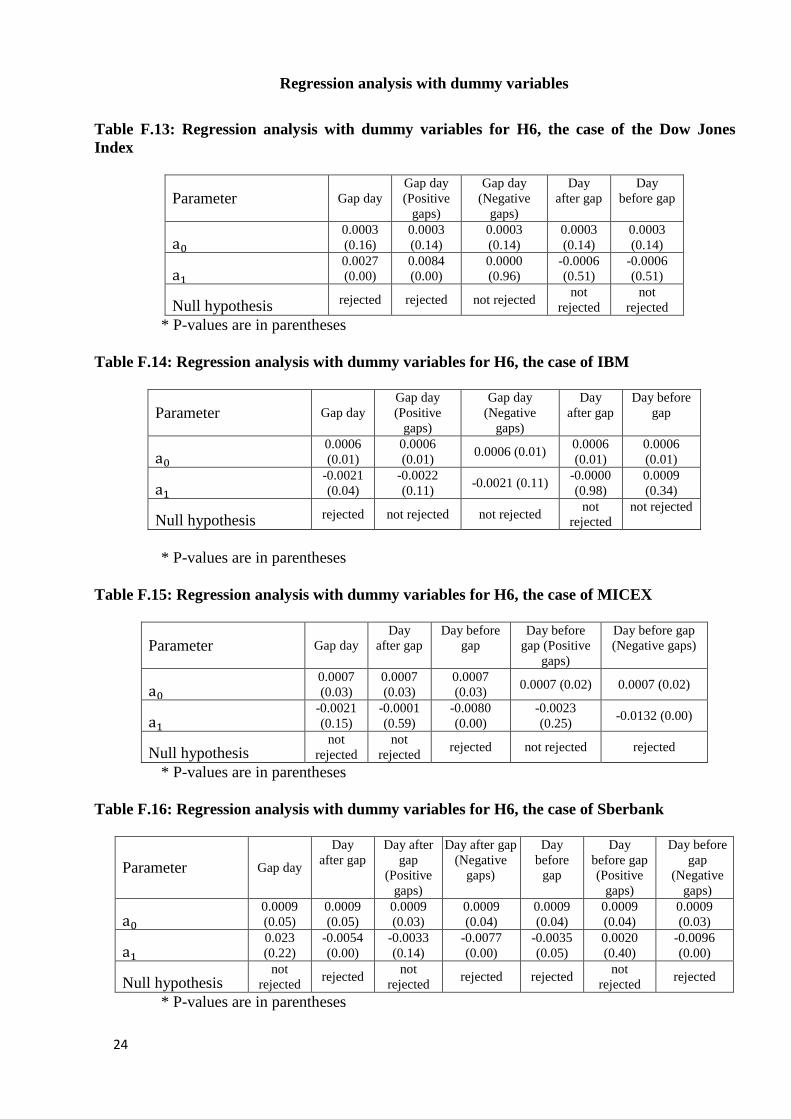
We also run regressions including a dummy variable to identify statistically

significant differences between “normal” and “abnormal” periods:

Yt = a0 + a1Dt + εt (3)

where: 𝑌𝑡 – return in period t;

a0– mean return in a “normal” period;

a1– mean return in an “abnormal” period;

Dt – a dummy variable equal to 1 in “abnormal” periods and 0 in “normal”

periods;

εt – Random error term for period t.

The size, sign and statistical significance of the dummy coefficients provide

information about possible anomalies. When anomalies are detected using the

previous methods we examine whether they give rise to exploitable profit

opportunities using a trading robot approach. This considers the detected anomalies

from the point of view of a trader who is interested in making abnormal profits by

exploiting them. The trading robot simulates the actions of a trader according to an

algorithm (trading strategy). This is a programme in the MetaTrader terminal that

5

has been developed in MetaQuotes Language 4 (MQL4) and used for the

automation of analytical and trading processes. Trading robots (called experts in

MetaTrader) allow to analyse price data and manage trading activities on the basis

of the signals received. One of the biggest advantages of this approach is that a

wide range of parameters can be tested. Further, it incorporates in the analysis

transaction costs. A strategy resulting in a number of profitable trades > 50% and

positive total profits is seen as evidence of an exploitable market anomaly.

To make sure that the results we obtain are statistically different from the

random trading ones we carry out z-tests. A z-test compares the means from two

samples to see whether they come from the same population. In our case the first is

the average profit/loss factor of one trade applying the trading strategy, and the

second is equal to zero because random trading (without transaction costs) should

generate zero profit. The null hypothesis (H0) is that the mean is the same in both

samples, and the alternative (H1) that it is not. The computed values of the z-test

are compared with the critical one at the 5% significance level. Failure to reject H0

implies that there are no advantages from exploiting the trading strategy being

considered, whilst a rejection suggests that the adopted strategy can generate

abnormal profits.

4. Empirical Results

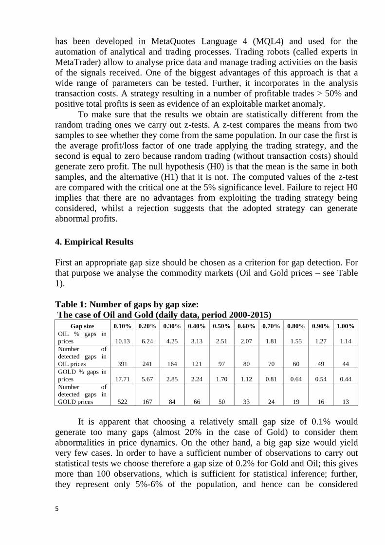
First an appropriate gap size should be chosen as a criterion for gap detection. For

that purpose we analyse the commodity markets (Oil and Gold prices – see Table

1).

Table 1: Number of gaps by gap size:

The case of Oil and Gold (daily data, period 2000-2015)

Gap size 0.10% 0.20% 0.30% 0.40% 0.50% 0.60% 0.70% 0.80% 0.90% 1.00%

OIL % gaps in

prices 10.13 6.24 4.25 3.13 2.51 2.07 1.81 1.55 1.27 1.14

Number of

detected gaps in

OIL prices 391 241 164 121 97 80 70 60 49 44

GOLD % gaps in

prices 17.71 5.67 2.85 2.24 1.70 1.12 0.81 0.64 0.54 0.44

Number of

detected gaps in

GOLD prices 522 167 84 66

50 33 24 19 16 13

It is apparent that choosing a relatively small gap size of 0.1% would

generate too many gaps (almost 20% in the case of Gold) to consider them

abnormalities in price dynamics. On the other hand, a big gap size would yield

very few cases. In order to have a sufficient number of observations to carry out

statistical tests we choose therefore a gap size of 0.2% for Gold and Oil; this gives

more than 100 observations, which is sufficient for statistical inference; further,

they represent only 5%-6% of the population, and hence can be considered

6

anomalies. The selected gap size, generating the same percentage of gaps (5-6%)

in the data set, is instead 8% for the Russian stock market.

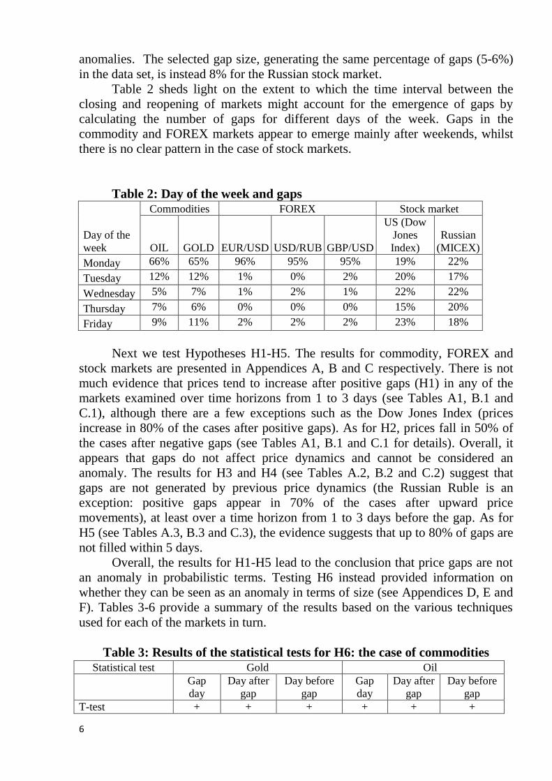
Table 2 sheds light on the extent to which the time interval between the

closing and reopening of markets might account for the emergence of gaps by

calculating the number of gaps for different days of the week. Gaps in the

commodity and FOREX markets appear to emerge mainly after weekends, whilst

there is no clear pattern in the case of stock markets.

Table 2: Day of the week and gaps

Day of the

week

Commodities FOREX Stock market

OIL GOLD EUR/USD USD/RUB GBP/USD

US (Dow

Jones

Index)

Russian

(MICEX)

Monday 66% 65% 96% 95% 95% 19% 22%

Tuesday 12% 12% 1% 0% 2% 20% 17%

Wednesday 5% 7% 1% 2% 1% 22% 22%

Thursday 7% 6% 0% 0% 0% 15% 20%

Friday 9% 11% 2% 2% 2% 23% 18%

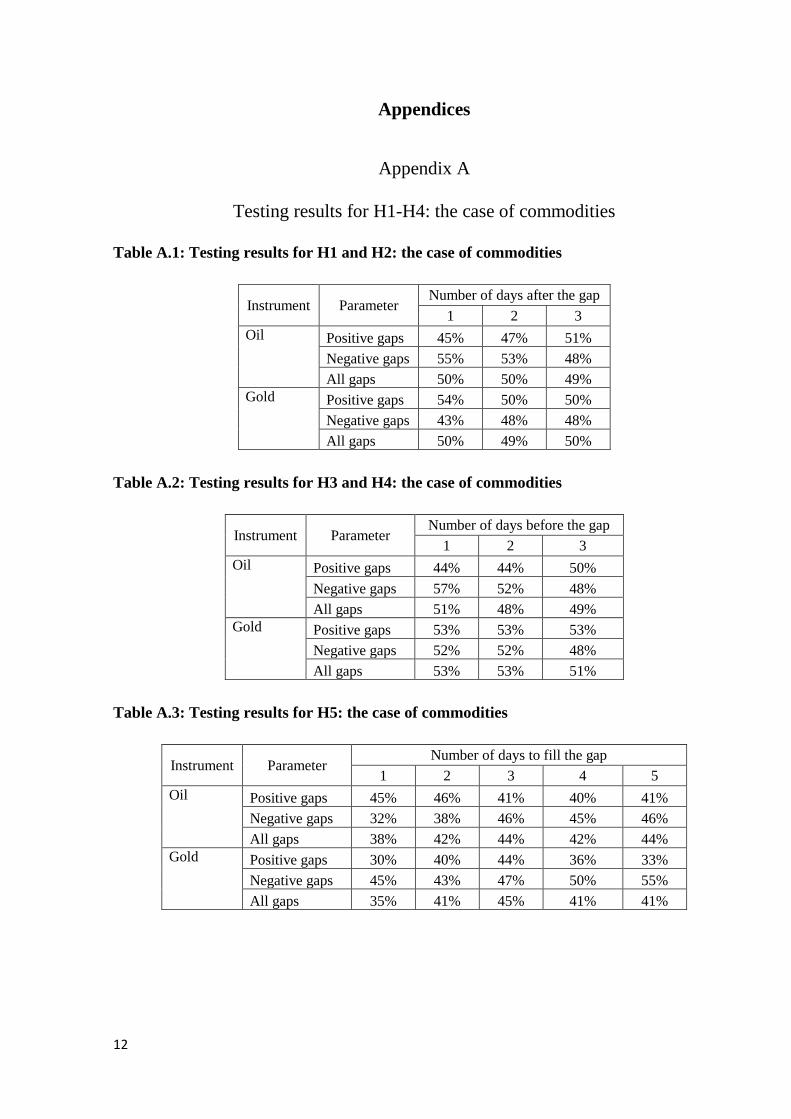
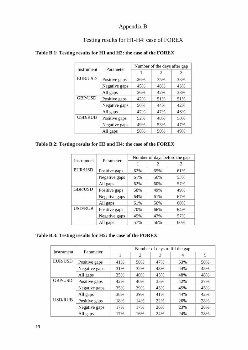
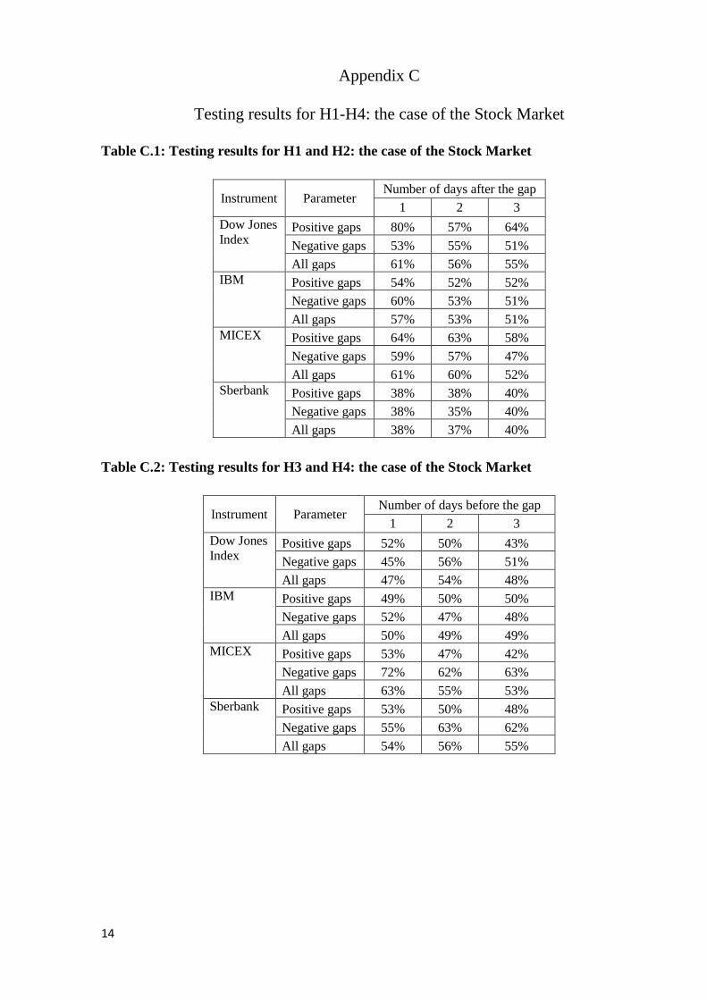
Next we test Hypotheses H1-H5. The results for commodity, FOREX and

stock markets are presented in Appendices A, B and C respectively. There is not

much evidence that prices tend to increase after positive gaps (H1) in any of the

markets examined over time horizons from 1 to 3 days (see Tables A1, B.1 and

C.1), although there are a few exceptions such as the Dow Jones Index (prices

increase in 80% of the cases after positive gaps). As for H2, prices fall in 50% of

the cases after negative gaps (see Tables A1, B.1 and C.1 for details). Overall, it

appears that gaps do not affect price dynamics and cannot be considered an

anomaly. The results for H3 and H4 (see Tables A.2, B.2 and C.2) suggest that

gaps are not generated by previous price dynamics (the Russian Ruble is an

exception: positive gaps appear in 70% of the cases after upward price

movements), at least over a time horizon from 1 to 3 days before the gap. As for

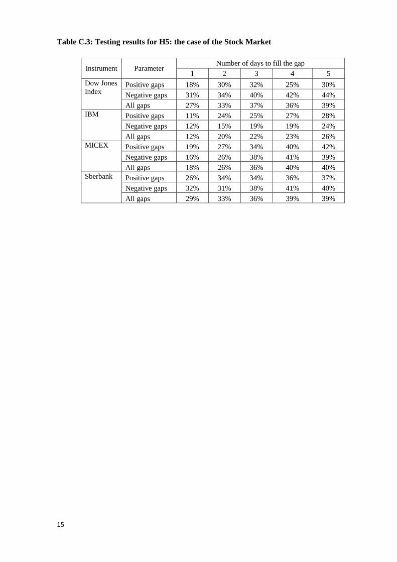
H5 (see Tables A.3, B.3 and C.3), the evidence suggests that up to 80% of gaps are

not filled within 5 days.

Overall, the results for H1-H5 lead to the conclusion that price gaps are not

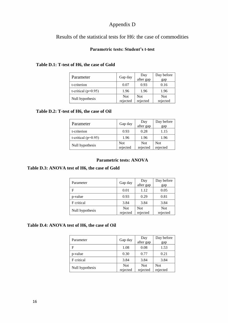
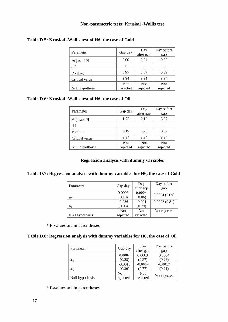
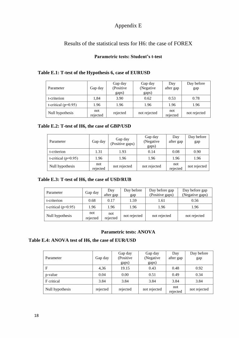
an anomaly in probabilistic terms. Testing H6 instead provided information on

whether they can be seen as an anomaly in terms of size (see Appendices D, E and

F). Tables 3-6 provide a summary of the results based on the various techniques

used for each of the markets in turn.

Table 3: Results of the statistical tests for H6: the case of commodities Statistical test Gold Oil

Gap

day

Day after

gap

Day before

gap

Gap

day

Day after

gap

Day before

gap

T-test + + + + + +

7

ANOVA test + + + + + +

Kruskal -Wallis test + + + + + +

Regression analysis

with dummy

variables

+ + + + + +

* ”+” – null hypothesis not rejected, “-” - null hypothesis rejected

As can be seen, there is no indication that gaps play any role in the case of

commodity prices.

Table 4: Results of the statistic tests for the H6: case of FOREX

Statistical test EURUSD GBPUSD USDRUB

Gap

day

Day

after

gap

Day

before

gap

Gap

day

Day

after

gap

Day

before

gap

Gap

day

Day

after

gap

Day

before

gap

T-test + + + + + + + + +

ANOVA test - + + - + + + + -

Kruskal -Wallis test + + + + + + + + -

Regression analysis

with dummy

variables

- + + - + + + + -


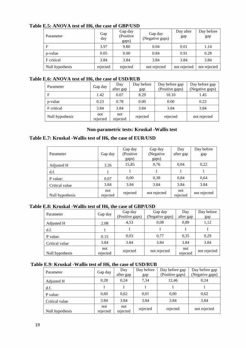
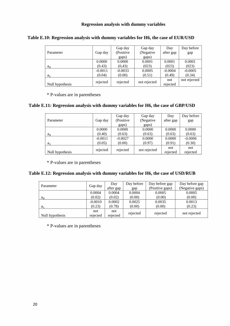
In the FOREX (EUR/USD and GBP/USD exchange rates) instead it is clear

that price dynamics in gap days differ from normal ones; specifically, they are

affected by positive gaps (see Tables E.1, E.2, E.4, E.5, E.7, E.8 for details). Since

the sign of the dummy coefficient in the regression is negative after a positive gap,

the following trading strategy should be tested to see if it is profitable: sell

and close the position at the end of the day. As for the EURUSD and GBPUSD

USD/RUB exchange rate, there is some evidence that price dynamics before gaps

are abnormal and might be generating them.

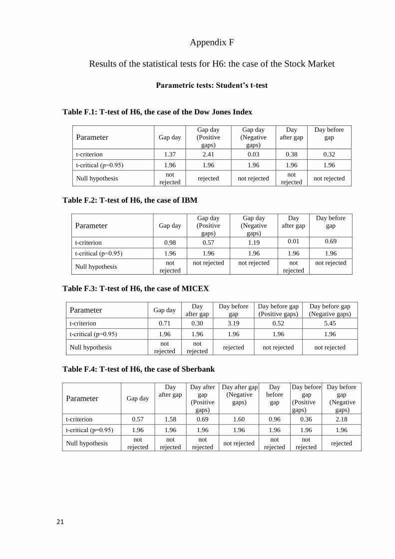
Table 5: Results of the statistic tests for the H6: the case of the US Stock

market Statistical test Dow Jones Index IBM

Gap

day

Day after

gap

Day before

gap Gap

day

Day after

gap

Day before

gap

T-test + + + + + +

ANOVA test - + + - + +

Kruskal -Wallis test + + + + + +

Regression analysis

with dummy

variables

- + + - + +


8

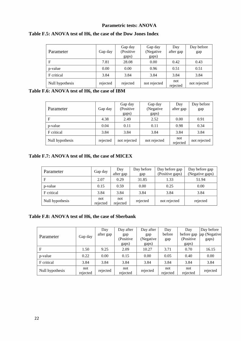
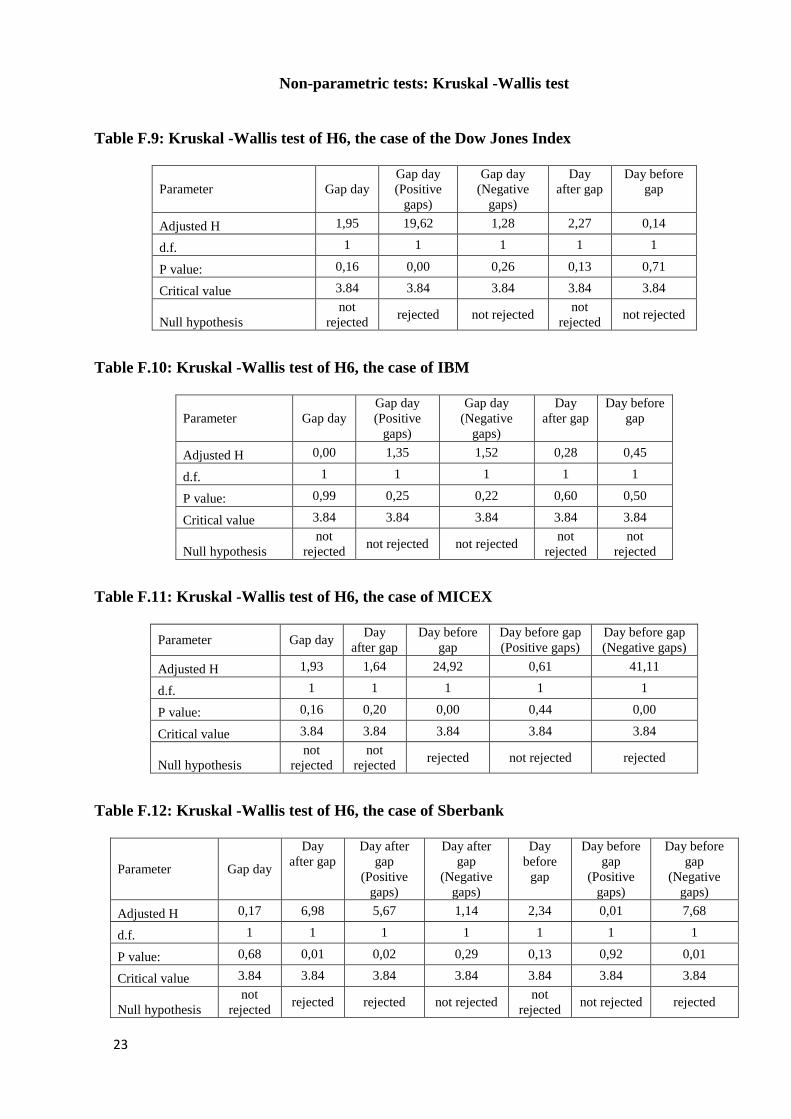
The results for the US stock market are mixed, but there is some evidence

that price dynamics in the gap day differs from normal ones. In case of the Dow

Jones Index when positive gaps emerge prices tend to increase, whilst the price of

IBM shares moves down after any gaps, whether positive or negative. Therefore

profitable trading strategies might be the following: in the case of the Dow Jones

index long positions should be opened after positive gaps; as for IBM shares, short

positions should be opened after any gaps. In both cases the opened positions

should be closed at the end of the day.

Table 6: Results of the statistical tests for the H6: the case of the Russian stock

market

Statistical test MICEX Sberbank

Gap

day

Day after

gap Day before

gap Gap

day

Day

after

gap

Day before

gap

T-test + + - + + +

ANOVA test + + - + - +

Kruskal -Wallis test + + - + - +

Regression analysis

with dummy

variables

+ + - + - +


The results for the Russian stock market differ from those for the US one,

possibly reflecting lower efficiency, but are consistent with those for the

USD/RUB exchange rate: abnormal price dynamics signal forthcoming gaps in

less efficient markets. In the specific case of Sberbank price dynamics differ from

normal ones only after a negative gap. Therefore a profitable trading strategy

would be to sell in the day after a negative gap, and to close the opened positions at

the end of the day.

Because the clearest evidence of abnormal price behaviour associated with

the emergence of gaps is found in the case of the FOREX, we implement for this

market a trading robot approach to test whether the trading strategy already

mentioned (sell the currency pair EUR/USD1 or GBP/USD after positive gaps and

close the position at the end of the day) is indeed profitable. The only parameter to

be set is the gap size, which is chosen using an optimisation procedure with 0.05%-

1% as the range of possible values and with 0.05% steps. The five most profitable

strategies are shown in Table 7.

1 EUR/USD or GBP/USD are currency pairs traded in the FOREX as financial instruments. To sell EUR/USD

(GBP?USD) means that the trader sells EUR (GBP) for USD, or equivalently buys USD for EUR (GBP). This dual

operation can be executed at once using the trading instruments EUR/USD and/or GBP/USD.

9

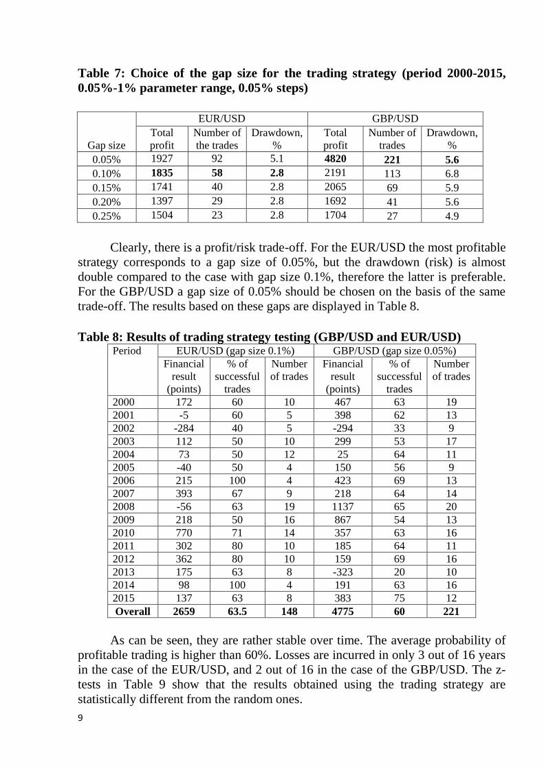
Table 7: Choice of the gap size for the trading strategy (period 2000-2015,

0.05%-1% parameter range, 0.05% steps)

Gap size

EUR/USD GBP/USD

Total

profit

Number of

the trades

Drawdown,

%

Total

profit

Number of

trades

Drawdown,

%

0.05% 1927 92 5.1 4820 221 5.6

0.10% 1835 58 2.8 2191 113 6.8

0.15% 1741 40 2.8 2065 69 5.9

0.20% 1397 29 2.8 1692 41 5.6

0.25% 1504 23 2.8 1704 27 4.9

Clearly, there is a profit/risk trade-off. For the EUR/USD the most profitable

strategy corresponds to a gap size of 0.05%, but the drawdown (risk) is almost

double compared to the case with gap size 0.1%, therefore the latter is preferable.

For the GBP/USD a gap size of 0.05% should be chosen on the basis of the same

trade-off. The results based on these gaps are displayed in Table 8.

Table 8: Results of trading strategy testing (GBP/USD and EUR/USD) Period EUR/USD (gap size 0.1%) GBP/USD (gap size 0.05%)

Financial

result

(points)

% of

successful

trades

Number

of trades

Financial

result

(points)

% of

successful

trades

Number

of trades

2000 172 60 10 467 63 19

2001 -5 60 5 398 62 13

2002 -284 40 5 -294 33 9

2003 112 50 10 299 53 17

2004 73 50 12 25 64 11

2005 -40 50 4 150 56 9

2006 215 100 4 423 69 13

2007 393 67 9 218 64 14

2008 -56 63 19 1137 65 20

2009 218 50 16 867 54 13

2010 770 71 14 357 63 16

2011 302 80 10 185 64 11

2012 362 80 10 159 69 16

2013 175 63 8 -323 20 10

2014 98 100 4 191 63 16

2015 137 63 8 383 75 12

Overall 2659 63.5 148 4775 60 221

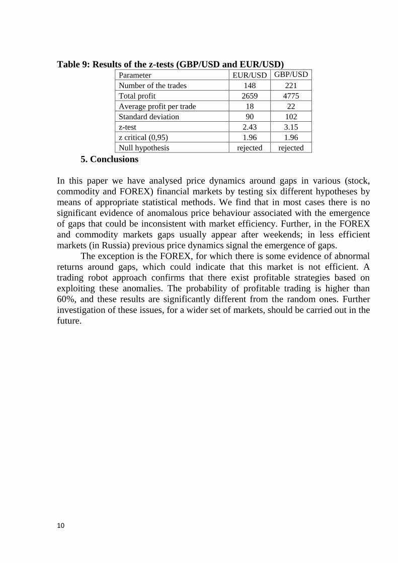
As can be seen, they are rather stable over time. The average probability of

profitable trading is higher than 60%. Losses are incurred in only 3 out of 16 years

in the case of the EUR/USD, and 2 out of 16 in the case of the GBP/USD. The z-

tests in Table 9 show that the results obtained using the trading strategy are

statistically different from the random ones.

10

Table 9: Results of the z-tests (GBP/USD and EUR/USD) Parameter EUR/USD GBP/USD

Number of the trades 148 221

Total profit 2659 4775

Average profit per trade 18 22

Standard deviation 90 102

z-test 2.43 3.15

z critical (0,95) 1.96 1.96

Null hypothesis rejected rejected

5. Conclusions

In this paper we have analysed price dynamics around gaps in various (stock,

commodity and FOREX) financial markets by testing six different hypotheses by

means of appropriate statistical methods. We find that in most cases there is no

significant evidence of anomalous price behaviour associated with the emergence

of gaps that could be inconsistent with market efficiency. Further, in the FOREX

and commodity markets gaps usually appear after weekends; in less efficient

markets (in Russia) previous price dynamics signal the emergence of gaps.

The exception is the FOREX, for which there is some evidence of abnormal

returns around gaps, which could indicate that this market is not efficient. A

trading robot approach confirms that there exist profitable strategies based on

exploiting these anomalies. The probability of profitable trading is higher than

60%, and these results are significantly different from the random ones. Further

investigation of these issues, for a wider set of markets, should be carried out in the

future.

11

References

Akerlof, G.A., and Shiller, R.J., 2009, Animal Spirits: How Human Psychology

Drives the Economy, and Why It Matters for Global Capitalism. Princeton

University Press, 2009, 248 p.

Caporale, G. M., Gil-Alana, L. Plastun, A. and Makarenko, I., 2016, Intraday

Anomalies and Market Efficiency: A Trading Robot Analysis. Computational

Economics, 47 (2), 275-295.

Fama, E., 1970, Efficient Capital Markets: A Review of Theory and Empirical

Work. Journal of Finance, 25, 383-417.

Fortune, P., 1998, Weekends can be rough: Revisiting the weekend effect in stock

prices. Federal Reserve Bank of Boston. Working Paper No. 98-6.

Fortune, P., 1999, Are stock returns different over weekends? а jump diffusion

analysis of the «weekend effect». New England Economic Review, September-

October, 3-19.

Jacobsen, B., Mamun, A., and Visaltanachoti, N., 2005, Seasonal, Size and Value

Anomalies. Working Paper, Massey University, University of Saskatchewan.

Jensen, M. C., 1978, Some Anomalous Evidence Regarding Market Efficiency.

Journal of Financial Economics, 6, 95-102.

Lo, A., 1991, Long-term Memory in Stock Market Prices. Econometrica, 59 (5),

1279–1313.

Mandelbrot, B., 1963, “The variation of certain speculative prices”, Journal of

Business, 36 (4), 394-419.

Olson, D., N. Chou, and C. Mossman, 2010, Stages in the life of the weekend

effect, Journal of Financial Economics, 21, 542-422.

Schwert G. W., 2003, Anomalies and market efficiency. Handbook of the

Economics of Finance, in: G.M. Constantinides & M. Harris & R. M. Stulz (ed.),

Handbook of the Economics of Finance, edition 1, volume 1, chapter 15, pages

939-974 Elsevier.

Shiller, R. J., 2000, Irrational Exuberance. Princeton University Press, 2000, 296 p.

12

Appendices

Appendix A

Testing results for H1-H4: the case of commodities

Table A.1: Testing results for H1 and H2: the case of commodities

Instrument Parameter Number of days after the gap

1 2 3

Oil Positive gaps 45% 47% 51%

Negative gaps 55% 53% 48%

All gaps 50% 50% 49%

Gold Positive gaps 54% 50% 50%


All gaps 50% 49% 50%

Table A.2: Testing results for H3 and H4: the case of commodities

Instrument Parameter Number of days before the gap

1 2 3

Oil Positive gaps 44% 44% 50%


All gaps 51% 48% 49%

Gold Positive gaps 53% 53% 53%


All gaps 53% 53% 51%

Table A.3: Testing results for H5: the case of commodities

Instrument Parameter Number of days to fill the gap

1 2 3 4 5

Oil Positive gaps 45% 46% 41% 40% 41%

Negative gaps 32% 38% 46% 45% 46%

All gaps 38% 42% 44% 42% 44%

Gold Positive gaps 30% 40% 44% 36% 33%

Negative gaps 45% 43% 47% 50% 55%

All gaps 35% 41% 45% 41% 41%

13

Appendix B

Testing results for H1-H4: case of FOREX

Table B.1: Testing results for H1 and H2: the case of the FOREX

Instrument Parameter Number of the days after gap

1 2 3

EUR/USD Positive gaps 26% 35% 33%


All gaps 36% 42% 38%

GBP/USD Positive gaps 42% 51% 51%


All gaps 47% 47% 46%

USD/RUB Positive gaps 52% 48% 50%


All gaps 50% 50% 49%

Table B.2: Testing results for H3 and H4: the case of the FOREX


1 2 3

EUR/USD Positive gaps 62% 65% 61%


All gaps 62% 60% 57%

GBP/USD Positive gaps 58% 49% 49%


All gaps 61% 56% 60%

USD/RUB Positive gaps 70% 66% 64%


All gaps 57% 56% 60%

Table B.3: Testing results for H5: the case of the FOREX


1 2 3 4 5

EUR/USD Positive gaps 41% 50% 47% 53% 50%

Negative gaps 31% 32% 43% 44% 45%

All gaps 35% 40% 45% 48% 48%

GBP/USD Positive gaps 42% 40% 35% 42% 37%

Negative gaps 35% 39% 45% 45% 45%

All gaps 38% 39% 41% 44% 42%

USD/RUB Positive gaps 18% 14% 22% 26% 28%

Negative gaps 17% 17% 26% 23% 28%

All gaps 17% 16% 24% 24% 28%

14

Appendix C

Testing results for H1-H4: the case of the Stock Market

Table C.1: Testing results for H1 and H2: the case of the Stock Market

Instrument Parameter Number of days after the gap

1 2 3

Dow Jones

Index Positive gaps 80% 57% 64%


All gaps 61% 56% 55%

IBM Positive gaps 54% 52% 52%


All gaps 57% 53% 51%

MICEX Positive gaps 64% 63% 58%


All gaps 61% 60% 52%

Sberbank Positive gaps 38% 38% 40%


All gaps 38% 37% 40%

Table C.2: Testing results for H3 and H4: the case of the Stock Market


1 2 3

Dow Jones

Index Positive gaps 52% 50% 43%


All gaps 47% 54% 48%

IBM Positive gaps 49% 50% 50%


All gaps 50% 49% 49%

MICEX Positive gaps 53% 47% 42%


All gaps 63% 55% 53%

Sberbank Positive gaps 53% 50% 48%


All gaps 54% 56% 55%

15

Table C.3: Testing results for H5: the case of the Stock Market


1 2 3 4 5

Dow Jones

Index Positive gaps 18% 30% 32% 25% 30%

Negative gaps 31% 34% 40% 42% 44%

All gaps 27% 33% 37% 36% 39%

IBM Positive gaps 11% 24% 25% 27% 28%

Negative gaps 12% 15% 19% 19% 24%

All gaps 12% 20% 22% 23% 26%

MICEX Positive gaps 19% 27% 34% 40% 42%

Negative gaps 16% 26% 38% 41% 39%

All gaps 18% 26% 36% 40% 40%

Sberbank Positive gaps 26% 34% 34% 36% 37%

Negative gaps 32% 31% 38% 41% 40%

All gaps 29% 33% 36% 39% 39%

16

Appendix D

Results of the statistical tests for H6: the case of commodities

Parametric tests: Student’s t-test

Table D.1: T-test of H6, the case of Gold

Parameter Gap day Day

after gap

Day before

gap

t-criterion 0.07 0.93 0.16

t-critical (р=0.95) 1.96 1.96 1.96

Null hypothesis Not

rejected

Not

rejected

Not

rejected

Table D.2: T-test of H6, the case of Oil


after gap

Day before

gap

t-criterion 0.93 0.28 1.15

t-critical (р=0.95) 1.96 1.96 1.96

Null hypothesis Not

rejected

Not

rejected

Not

rejected

Parametric tests: ANOVA

Table D.3: ANOVA test of H6, the case of Gold


after gap

Day before

gap

F 0.01 1.12 0.05

p-value 0.93 0.29 0.81

F critical 3.84 3.84 3.84

Null hypothesis Not

rejected

Not

rejected

Not

rejected

Table D.4: ANOVA test of H6, the case of Oil


after gap

Day before

gap

F 1.08 0.08 1.53

p-value 0.30 0.77 0.21

F critical 3.84 3.84 3.84

Null hypothesis Not

rejected

Not

rejected

Not

rejected

17

Non-parametric tests: Kruskal -Wallis test

Table D.5: Kruskal -Wallis test of H6, the case of Gold


after gap

Day before

gap

Adjusted H 0.00 2,81 0,02

d.f. 1 1 1

P value: 0.97 0,09 0,89

Critical value 3.84 3.84 3.84

Null hypothesis

Not

rejected

Not

rejected

Not

rejected

Table D.6: Kruskal -Wallis test of H6, the case of Oil


after gap

Day before

gap

Adjusted H 1,72 0,10 3,27

d.f. 1 1 1

P value: 0,19 0,76 0,07

Critical value 3.84 3.84 3.84

Null hypothesis

Not

rejected

Not

rejected

Not

rejected

Regression analysis with dummy variables

Table D.7: Regression analysis with dummy variables for H6, the case of Gold


after gap

Day before

gap

a0

0.0003

(0.10)

0.0004

(0.06) 0.0004 (0.09)

a1

-0.086

(0.93)

-0.001

(0.29)

0.0002 (0.81)

Null hypothesis

Not

rejected

Not

rejected

Not rejected

* P-values are in parentheses

Table D.8: Regression analysis with dummy variables for H6, the case of Oil


after gap

Day before

gap

a0

0.0004

(0.28)

0.0003

(0.37)

0.0004

(0.26)

a1

-0.0015

(0.30)

-0.0004

(0.77)

-0.0017

(0.21)

Null hypothesis

Not

rejected

Not

rejected Not rejected


18

Appendix E

Results of the statistical tests for H6: the case of FOREX


Table E.1: T-test of the Hypothesis 6, case of EURUSD

Parameter Gap day

Gap day

(Positive

gaps)

Gap day

(Negative

gaps)

Day

after gap

Day before

gap

t-criterion 1,84 3.90 0.62 0.53 0.78

t-critical (р=0.95) 1.96 1.96 1.96 1.96 1.96

Null hypothesis not

rejected rejected not rejected

not

rejected not rejected

Table E.2: T-test of H6, the case of GBP/USD

Parameter Gap day Gap day

(Positive gaps)

Gap day

(Negative

gaps)

Day

after gap

Day before

gap

t-criterion 1.31 1.93 0.14 0.08 0.90

t-critical (р=0.95) 1.96 1.96 1.96 1.96 1.96

Null hypothesis not

rejected not rejected not rejected

not


Table E.3: T-test of H6, the case of USD/RUB


after gap

Day before

gap

Day before gap

(Positive gaps)

Day before gap

(Negative gaps)

t-criterion 0.68 0.17 1.59 1.61 0.56

t-critical (р=0.95) 1.96 1.96 1.96 1.96 1.96

Null hypothesis not

rejected

not

rejected not rejected not rejected not rejected


Table E.4: ANOVA test of H6, the case of EUR/USD

Parameter Gap day

Gap day

(Positive

gaps)

Gap day

(Negative

gaps)

Day

after gap

Day before

gap

F 4,36 19.15 0.43 0.48 0.92

p-value 0.04 0.00 0.51 0.49 0.34

F critical 3.84 3.84 3.84 3.84 3.84

Null hypothesis rejected rejected not rejected not


19

Table E.5: ANOVA test of H6, the case of GBP/USD

Parameter Gap

day

Gap day

(Positive

gaps)

Gap day

(Negative gaps)

Day after

gap

Day before

gap

F 3.97 9.80 0.04 0.01 1.14

p-value 0.05 0.00 0.84 0.91 0.28

F critical 3.84 3.84 3.84 3.84 3.84

Null hypothesis rejected rejected not rejected not rejected not rejected

Table E.6: ANOVA test of H6, the case of USD/RUB


after gap

Day before

gap

Day before gap

(Positive gaps)

Day before gap

(Negative gaps)

F 1.42 0.07 8.29 10.10 1.45

p-value 0.23 0.78 0.00 0.00 0.23

F critical 3.84 3.84 3.84 3.84 3.84

Null hypothesis not

rejected

not

rejected rejected rejected not rejected


Table E.7: Kruskal -Wallis test of H6, the case of EUR/USD

Parameter Gap day

Gap day

(Positive

gaps)

Gap day

(Negative

gaps)

Day

after gap

Day before

gap

Adjusted H 3.26 15,85 0,76 0,04 0,22

d.f. 1 1 1 1 1

P value: 0.07 0,00 0,38 0,84 0,64

Critical value 3.84 3.84 3.84 3.84 3.84

Null hypothesis

not


not


Table E.8: Kruskal -Wallis test of H6, the case of GBP/USD

Parameter Gap day Gap day

(Positive gaps)

Gap day

(Negative gaps)

Day

after gap

Day before

gap

Adjusted H 2.08 4,53 0,08 0,89 1,12

d.f. 1 1 1 1 1

P value: 0.15 0,03 0,77 0,35 0,29

Critical value 3.84 3.84 3.84 3.84 3.84

Null hypothesis

not


not


Table E.9: Kruskal -Wallis test of H6, the case of USD/RUB


after gap

Day before

gap

Day before gap

(Positive gaps)

Day before gap

(Negative gaps)

Adjusted H 0,28 0,24 7,34 12,46 0,24

d.f. 1 1 1 1 1

P value: 0,60 0,62 0,01 0,00 0,62

Critical value 3.84 3.84 3.84 3.84 3.84

Null hypothesis

not

rejected

not


20


Table E.10: Regression analysis with dummy variables for H6, the case of EUR/USD

Parameter Gap day

Gap day

(Positive

gaps)

Gap day

(Negative

gaps)

Day

after gap

Day before

gap

a0

0.0000

(0.43)

0.0000

(0,43)

0.0001

(023)

0.0001

(023)

0.0001

(023)

a1

-0.0011

(0.04)

-0.0033

(0.00)

0.0005

(0.51)

-0.0004

(0.49)

-0.0005

(0.34)

Null hypothesis rejected rejected not rejected

not

rejected

not rejected


Table E.11: Regression analysis with dummy variables for H6, the case of GBP/USD

Parameter Gap day

Gap day

(Positive

gaps)

Gap day

(Negative

gaps)

Day

after gap

Day before

gap

a0

0.0000

(0.40)

0.0000

(0.63)

0.0000

(0.63)

0.0000

(0.63)

0.0000

(0.63)

a1

-0.0011

(0.05)

-0.0027

(0.00)

0.0000

(0.97)

0.0000

(0.91)

-0.0006

(0.30)

Null hypothesis rejected rejected not rejected

not

rejected

not

rejected


Table E.12: Regression analysis with dummy variables for H6, the case of USD/RUB


after gap

Day before

gap

Day before gap

(Positive gaps)

Day before gap

(Negative gaps)

a0

0.0004

(0.02)

0.0004

(0.02)

0.0004

(0.00)

0.0005

(0.00)

0.0005

(0.00)

a1

-0.0010

(0.23)

0.0002

(0.78)

0.0025

(0.00)

0.0035

(0.00)

0.0013

(0.23)

Null hypothesis

not

rejected

not



21

Appendix F

Results of the statistical tests for H6: the case of the Stock Market


Table F.1: T-test of H6, the case of the Dow Jones Index

Parameter Gap day

Gap day

(Positive

gaps)

Gap day

(Negative

gaps)

Day

after gap

Day before

gap

t-criterion 1.37 2.41 0.03 0.38 0.32

t-critical (р=0.95) 1.96 1.96 1.96 1.96 1.96

Null hypothesis not


not


Table F.2: T-test of H6, the case of IBM

Parameter Gap day

Gap day

(Positive

gaps)

Gap day

(Negative

gaps)

Day

after gap

Day before

gap

t-criterion 0.98 0.57 1.19 0.01 0.69

t-critical (р=0.95) 1.96 1.96 1.96 1.96 1.96

Null hypothesis not

rejected

not rejected not rejected not

rejected

not rejected

Table F.3: T-test of H6, the case of MICEX


after gap

Day before

gap

Day before gap

(Positive gaps)

Day before gap

(Negative gaps)

t-criterion 0.71 0.30 3.19 0.52 5.45

t-critical (р=0.95) 1.96 1.96 1.96 1.96 1.96

Null hypothesis not

rejected

not

rejected rejected not rejected not rejected

Table F.4: T-test of H6, the case of Sberbank

Parameter Gap day

Day

after gap

Day after

gap

(Positive

gaps)

Day after gap

(Negative

gaps)

Day

before

gap

Day before

gap

(Positive

gaps)

Day before

gap

(Negative

gaps)

t-criterion 0.57 1.58 0.69 1.60 0.96 0.36 2.18

t-critical (р=0.95) 1.96 1.96 1.96 1.96 1.96 1.96 1.96

Null hypothesis not

rejected

not

rejected

not


not

rejected

not

rejected rejected

22


Table F.5: ANOVA test of H6, the case of the Dow Jones Index

Parameter Gap day

Gap day

(Positive

gaps)

Gap day

(Negative

gaps)

Day

after gap

Day before

gap

F 7.81 28.08 0.00 0.42 0.43

p-value 0.00 0.00 0.96 0.51 0.51

F critical 3.84 3.84 3.84 3.84 3.84



Table F.6: ANOVA test of H6, the case of IBM

Parameter Gap day

Gap day

(Positive

gaps)

Gap day

(Negative

gaps)

Day

after gap

Day before

gap

F 4.38 2.49 2.52 0.00 0.91

p-value 0.04 0.11 0.11 0.98 0.34

F critical 3.84 3.84 3.84 3.84 3.84

Null hypothesis rejected not rejected not rejected not


Table F.7: ANOVA test of H6, the case of MICEX


after gap

Day before

gap

Day before gap

(Positive gaps)

Day before gap

(Negative gaps)

F 2.07 0.29 31.85 1.33 51.94

p-value 0.15 0.59 0.00 0.25 0.00

F critical 3.84 3.84 3.84 3.84 3.84

Null hypothesis not

rejected

not

rejected rejected not rejected rejected

Table F.8: ANOVA test of H6, the case of Sberbank

Parameter Gap day

Day

after gap

Day after

gap

(Positive

gaps)

Day after

gap

(Negative

gaps)

Day

before

gap

Day

before gap

(Positive

gaps)

Day before

gap (Negative

gaps)

F 1.50 9.25 2.09 10.27 3.71 0.70 16.15

p-value 0.22 0.00 0.15 0.00 0.05 0.40 0.00

F critical 3.84 3.84 3.84 3.84 3.84 3.84 3.84

Null hypothesis not

rejected rejected

not

rejected rejected

not

rejected

not

rejected rejected

23


Table F.9: Kruskal -Wallis test of H6, the case of the Dow Jones Index

Parameter Gap day

Gap day

(Positive

gaps)

Gap day

(Negative

gaps)

Day

after gap

Day before

gap

Adjusted H 1,95 19,62 1,28 2,27 0,14

d.f. 1 1 1 1 1

P value: 0,16 0,00 0,26 0,13 0,71

Critical value 3.84 3.84 3.84 3.84 3.84

Null hypothesis

not


not


Table F.10: Kruskal -Wallis test of H6, the case of IBM

Parameter Gap day

Gap day

(Positive

gaps)

Gap day

(Negative

gaps)

Day

after gap

Day before

gap

Adjusted H 0,00 1,35 1,52 0,28 0,45

d.f. 1 1 1 1 1

P value: 0,99 0,25 0,22 0,60 0,50

Critical value 3.84 3.84 3.84 3.84 3.84

Null hypothesis

not

rejected not rejected not rejected

not

rejected

not

rejected

Table F.11: Kruskal -Wallis test of H6, the case of MICEX


after gap

Day before

gap

Day before gap

(Positive gaps)

Day before gap

(Negative gaps)

Adjusted H 1,93 1,64 24,92 0,61 41,11

d.f. 1 1 1 1 1

P value: 0,16 0,20 0,00 0,44 0,00

Critical value 3.84 3.84 3.84 3.84 3.84

Null hypothesis

not

rejected

not


Table F.12: Kruskal -Wallis test of H6, the case of Sberbank

Parameter Gap day

Day

after gap

Day after

gap

(Positive

gaps)

Day after

gap

(Negative

gaps)

Day

before

gap

Day before

gap

(Positive

gaps)

Day before

gap

(Negative

gaps)

Adjusted H 0,17 6,98 5,67 1,14 2,34 0,01 7,68

d.f. 1 1 1 1 1 1 1

P value: 0,68 0,01 0,02 0,29 0,13 0,92 0,01

Critical value 3.84 3.84 3.84 3.84 3.84 3.84 3.84

Null hypothesis

not


not

rejected not rejected rejected

24


Table F.13: Regression analysis with dummy variables for H6, the case of the Dow Jones

Index

Parameter Gap day

Gap day

(Positive

gaps)

Gap day

(Negative

gaps)

Day

after gap

Day

before gap

a0 0.0003

(0.16)

0.0003

(0.14)

0.0003

(0.14)

0.0003

(0.14)

0.0003

(0.14)

a1 0.0027

(0.00)

0.0084

(0.00)

0.0000

(0.96)

-0.0006

(0.51)

-0.0006

(0.51)


rejected

not

rejected


Table F.14: Regression analysis with dummy variables for H6, the case of IBM

Parameter Gap day

Gap day

(Positive

gaps)

Gap day

(Negative

gaps)

Day

after gap

Day before

gap

a0 0.0006

(0.01)

0.0006

(0.01) 0.0006 (0.01)

0.0006

(0.01)

0.0006

(0.01)

a1 -0.0021

(0.04)

-0.0022

(0.11) -0.0021 (0.11)

-0.0000

(0.98)

0.0009

(0.34)

Null hypothesis rejected not rejected not rejected not

rejected

not rejected


Table F.15: Regression analysis with dummy variables for H6, the case of MICEX

Parameter Gap day

Day

after gap

Day before

gap

Day before

gap (Positive

gaps)

Day before gap

(Negative gaps)

a0 0.0007

(0.03)

0.0007

(0.03)

0.0007

(0.03) 0.0007 (0.02) 0.0007 (0.02)

a1 -0.0021

(0.15)

-0.0001

(0.59)

-0.0080

(0.00)

-0.0023

(0.25) -0.0132 (0.00)

Null hypothesis not

rejected

not



Table F.16: Regression analysis with dummy variables for H6, the case of Sberbank

Parameter Gap day

Day

after gap

Day after

gap

(Positive

gaps)

Day after gap

(Negative

gaps)

Day

before

gap

Day

before gap

(Positive

gaps)

Day before

gap

(Negative

gaps)

a0 0.0009

(0.05)

0.0009

(0.05)

0.0009

(0.03)

0.0009

(0.04)

0.0009

(0.04)

0.0009

(0.04)

0.0009

(0.03)

a1 0.023

(0.22)

-0.0054

(0.00)

-0.0033

(0.14)

-0.0077

(0.00)

-0.0035

(0.05)

0.0020

(0.40)

-0.0096

(0.00)

Null hypothesis not

rejected rejected

not

rejected rejected rejected

not

rejected rejected


Documents

g Price Gaps: Another Market Anomaly? in · PDF filePRICE GAPS: ANOTHER MARKET ANOMALY? ... (Student’s t-tests, ... are compared with the critical one at the 5% significance level