2

AN UPDATE OF OECD LEADING INDICATORS *

G. Petit, G. Salou, P. Beziz and C. DegainSTD/MEI

The partial study being presented here is a first step towards a more comprehensive update of the systemof OECD leading indicators. While the system has worked relatively well since it was set up in its currentform (see in particular [1] and [4]), it would be useful to examine its actual performance and, wherenecessary, take a fresh look at its methodological foundations.

The OECD leading indicators were developed by a working party composed of Secretariat staff andnational experts and were based on work by the National Bureau of Economic Research (NBER) of theUnited States (see [5]: Introduction and Part A). The working party's dissolution in 1981 did not end thecontacts, however, since the principle of ad hoc meetings was adopted thereafter. Following the last suchmeeting, which was held in September 1984, the OECD leading indicators were published in their presentform in late 1987, in the Main Economic Indicators series, preceded by a publication on Sources andMethods ([5])1.

A monthly newsletter on the leading indicators computed by the OECD was also distributed in the 1980sfor in-house use by the Secretariat and Member country governments.

Since then, nearly ten years have gone by without major changes, primarily because the system has beenoperating fairly smoothly, but also because the Secretariat's programme of work and resource constraintshave until now precluded the idea of major work. Enough time has elapsed to look at how the OECDleading indicators have actually evolved and to review any relevant innovations by the Member countries.

The purpose of this study is to provide a basis for discussion of the first of these items. It has beenprepared entirely on the basis of data available in June 1996 and updated in the Main Economic Indicatorsdatabase.

Over the past three years, the OECD has welcomed new countries. We have formulated a leadingindicator of industrial production in Mexico, in particular to ascertain whether it would have beenpossible, and how far in advance, to predict the sudden economic reversal that took place in late 1994.This indicator is presented below and could ultimately be published in Main Economic Indicators,providing that the data used to compute it are updated regularly by the national statistics agencies. Theindicator's performance over a ten-year period is satisfactory.

To provide useful signals, quality updates and regular contacts with the Secretariat's statisticscorrespondents in the Member countries are essential. Over the past ten years, supply of some

* The authors would like to express their appreciation, in particular, to Martine Durand and Paul van den

Noord, of the OECD Economics Department, and to Béatrice du Boys, of the OECD StatisticsDirectorate, for their comments.

3

components of the leading indicators has been interrupted. Components can also become outdated, eitherbecause they have grown less relevant to the cycles of the reference series or because, over time, theirupdates have become less satisfactory for the computation of a composite index. Such cases, examples ofwhich are cited in the following study, point to a deterioration of quality.

In this study, the component series of the leading indicators of three countries have been updated oroverhauled: new composite indicators were introduced for the United States, in a relatively minor update,while German indicators were substantially simplified and the components of Norwegian indicators wererevised. Norway posed an additional problem with regard to the choice of a reference series. Generallythe industrial production is used as the reference series, and manufacturing output has so far been used forNorway.

Given the interest of outside users in the OECD leading indicators, the Statistics Directorate has added thecorresponding monthly newsletter, which had previously been available in-house only, to its list ofelectronic publications available on the Internet. This recent initiative considerably expands the number ofpotential users of the indicators.

It must be stressed that, while the resources available to the Main Economic Indicators Division duringpublication production periods have been adequate to make the replacements needed to compute theindicators, production priorities have rarely made it possible to carry out the extensive research suchreplacements warrant. Moreover, the formulation of leading indicators by means of the method presentedin [5] is a statistical exercise that has often proved useful, but it is also costly and time-consuming. Thisstudy was carried out on a short deadline, with no additional resources and within the priorities of theStatistics Directorate's programme of work2. It makes no claims to be either perfect or complete, and isopen to all your comments. We hope it will be of use in the substantive discussions of this first ad hocmeeting since 1984.

4

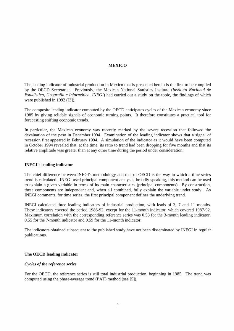
MEXICO

The leading indicator of industrial production in Mexico that is presented herein is the first to be compiledby the OECD Secretariat. Previously, the Mexican National Statistics Institute (Instituto Nacional deEstadística, Geografía e Informática, INEGI) had carried out a study on the topic, the findings of whichwere published in 1992 ([3]).

The composite leading indicator computed by the OECD anticipates cycles of the Mexican economy since1985 by giving reliable signals of economic turning points. It therefore constitutes a practical tool forforecasting shifting economic trends.

In particular, the Mexican economy was recently marked by the severe recession that followed thedevaluation of the peso in December 1994. Examination of the leading indicator shows that a signal ofrecession first appeared in February 1994. A simulation of the indicator as it would have been computedin October 1994 revealed that, at the time, its ratio to trend had been dropping for five months and that itsrelative amplitude was greater than at any other time during the period under consideration.

INEGI's leading indicator

The chief difference between INEGI's methodology and that of OECD is the way in which a time-seriestrend is calculated. INEGI used principal component analysis; broadly speaking, this method can be usedto explain a given variable in terms of its main characteristics (principal components). By construction,these components are independent and, when all combined, fully explain the variable under study. AsINEGI comments, for time series, the first principal component defines the underlying trend.

INEGI calculated three leading indicators of industrial production, with leads of 3, 7 and 11 months.These indicators covered the period 1986-92, except for the 11-month indicator, which covered 1987-92.Maximum correlation with the corresponding reference series was 0.53 for the 3-month leading indicator,0.55 for the 7-month indicator and 0.59 for the 11-month indicator.

The indicators obtained subsequent to the published study have not been disseminated by INEGI in regularpublications.

The OECD leading indicator

Cycles of the reference series

For the OECD, the reference series is still total industrial production, beginning in 1985. The trend wascomputed using the phase-average trend (PAT) method (see [5]).

5

All cycles detected in the industrial production series were also found in the gross domestic product (GDP)series3, except for a cycle of minor amplitude between January and July 1992.

Industrial production cycles generally lead or are coincident with those of GDP (see Table 1 and Figure 1).This confirms the choice of the industrial production series as the reference series for Mexico. It reflectsGDP trends and is available on a monthly basis, in contrast to the GDP series, which is computedquarterly.

Table 1: Comparison of GDP cycles3 with those of the reference series

Gross domestic product Industrial productionTurning point

dates (quarters)Amplitude Turning point

dates (months)Amplitude

Peaks Troughs % of trend Peaks Troughs % of trend

3/85 +2.8 7/85 + 5.074/86 -2.22 12/86 - 5.78

4/87 +1.05 9/87 + 2.783/88 -2.07 7/88 - 3.94

2/91 +2.36 8/90 + 1.941/92 - 2.60

7/92 + 3.042/93 -1.8 6/93 - 2.00

4/94 +3.72 8/94 + 6.392/95 -5.69 5/95 - 7.10

Figure 1: Ratio to trend for GDP3, 4 and the reference series4

Jan-85 Jan-86 Jan-87 Jan-88 Jan-89 Jan-90 Jan-91 Jan-92 Jan-93 Jan-94 Jan-95 Jan-960.9

0.95

1

1.05

1.1

Ratio to trend

Industrial Production Gross Domestic Product

Examination of the reference series shows four major periods reflecting the development of the Mexicaneconomy (see in particular [6]).

The period between July 1985 and July 1988 contained three phases of declining duration and relativeamplitude, each clearly in evidence at the outset (absolute relative amplitude greater than 5 per cent).

Between August 1988 and mid-1993, cycles were not very pronounced and had low relative amplitude.This reflected the government's economic policy, which combined a tight rein on public finances with

6

strict monetary policy in order to stabilise inflation at a level near that of Mexico's main economicpartners.

After 1993, implementation of economic reforms and an opening up to the outside world (membership ofthe North American market through NAFTA as of 1 January 1994) were followed by a policy ofexpansion. The phase between June 1993 and July 1994 was clearly pronounced (with a peak of relativeamplitude of 6.4 per cent).

Finally, the severe recession that followed devaluation of the peso on 20 December 1994 was reflected inthe industrial production series by a short (nine-month) phase with high amplitude (7 per cent of thetrend).

Component series of the leading indicator

The component series used to compute the OECD leading indicator were chosen after an examination of62 different time series, drawn primarily from the “Main Economic Indicators” database, but also fromINEGI's “Banco de datos” base and the Bank of Mexico's SINIEE database. A diskette version ofSINIEE as of 27 February 1996 (containing data to January 1996 at the latest) was used.

A large number of these series were rejected, because they lacked a relevant cyclical profile or because theamplitudes of the cycles they contained were out of proportion to the corresponding cycles of the referenceseries. The series had to do with the “real” economy (components of industrial production, wages, prices,construction costs, exports, etc., in terms of levels or differentials) or with financial data (the moneysupply, share prices, official reserves, peso/US dollar exchange rates, federal government deficits, etc.).

Moreover, it was impossible to test the cyclical behaviour of a great many series, either because data werenot available over a long enough period (e.g. the yield on “tesobonos”5) or because they were calculatedon an annual basis only (e.g. foreign investment in Mexico).

In the end, seven series were selected:

• Three net opinion series from the Bank of Mexico's business survey:− Employment: tendency;− Stocks of finished goods: tendency;− Production: tendency.

These three series relate to business opinion for the month of the survey, as compared with the previousmonth. It should be noted that the Bank of Mexico also questions businesses about the one-monthoutlook. The corresponding net opinions are not released, however, and it was not possible to test thesedata, which would be likely to yield a better lead on cycles of the reference series.

• Two series of financial rates:− Average cost to banks of managing deposits in national currency (costo promedio de captación en

moneda nacional, CPP).− US ten-year interest rates: interest rates on 10-year federal government bonds, as currently published

in Main Economic Indicators.

7

• The Real effective exchange rate calculated by the OECD Economics Department and also published inMain Economic Indicators. This rate is an indicator of competitiveness, which takes into account therelative importance of Mexico's competitors in thirty markets, and the relative importance of thosemarkets (see [2]).

• A series derived from INEGI's monthly industrial survey:− Monthly changes in manufacturing employment. These data are akin to employment tendency in

manufacturing (see above), which is a business survey series. Note that the level of manufacturingemployment is not relevant.

It should be noted that the US 10-year interest rate series is included from 1990, when its cyclicalbehaviour began to coincide with the industrial production series. All other series are included from 1985.

Main results

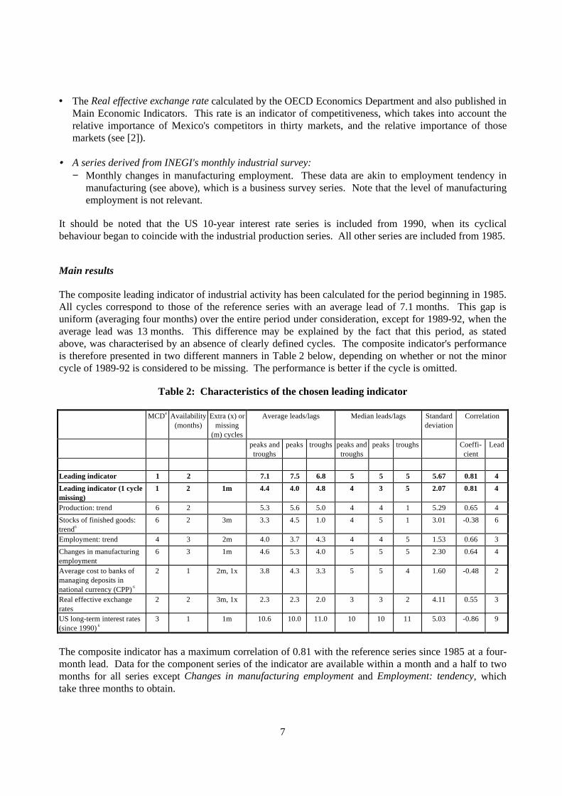
The composite leading indicator of industrial activity has been calculated for the period beginning in 1985.All cycles correspond to those of the reference series with an average lead of 7.1 months. This gap isuniform (averaging four months) over the entire period under consideration, except for 1989-92, when theaverage lead was 13 months. This difference may be explained by the fact that this period, as statedabove, was characterised by an absence of clearly defined cycles. The composite indicator's performanceis therefore presented in two different manners in Table 2 below, depending on whether or not the minorcycle of 1989-92 is considered to be missing. The performance is better if the cycle is omitted.

Table 2: Characteristics of the chosen leading indicator

MCD4 Availability(months)

Extra (x) ormissing

(m) cycles

Average leads/lags Median leads/lags Standarddeviation

Correlation

peaks andtroughs

peaks troughs peaks andtroughs

peaks troughs Coeffi-cient

Lead

Leading indicator 1 2 7.1 7.5 6.8 5 5 5 5.67 0.81 4

Leading indicator (1 cyclemissing)

1 2 1m 4.4 4.0 4.8 4 3 5 2.07 0.81 4

Production: trend 6 2 5.3 5.6 5.0 4 4 1 5.29 0.65 4

Stocks of finished goods:trend6

6 2 3m 3.3 4.5 1.0 4 5 1 3.01 -0.38 6

Employment: trend 4 3 2m 4.0 3.7 4.3 4 4 5 1.53 0.66 3

Changes in manufacturingemployment

6 3 1m 4.6 5.3 4.0 5 5 5 2.30 0.64 4

Average cost to banks ofmanaging deposits innational currency (CPP) 6

2 1 2m, 1x 3.8 4.3 3.3 5 5 4 1.60 -0.48 2

Real effective exchangerates

2 2 3m, 1x 2.3 2.3 2.0 3 3 2 4.11 0.55 3

US long-term interest rates(since 1990) 6

3 1 1m 10.6 10.0 11.0 10 10 11 5.03 -0.86 9

The composite indicator has a maximum correlation of 0.81 with the reference series since 1985 at a four-month lead. Data for the component series of the indicator are available within a month and a half to twomonths for all series except Changes in manufacturing employment and Employment: tendency, whichtake three months to obtain.

8

Figure 2: Leading indicator7 and reference series4, ratio to trend

Jan-85 Jan-86 Jan-87 Jan-88 Jan-89 Jan-90 Jan-91 Jan-92 Jan-93 Jan-94 Jan-95 Jan-960.85

0.9

0.95

1

1.05

1.1

Ratio to trend

Industrial Production Leading Indicator

Simulation of the December 1994 recession

The composite leading indicator announces the recession with a lead of six months (turning point inFebruary 1994). The indicator was recalculated as it would have been in October 1994, two months afterthe peak, assuming that, at the time, the databases used for the study had been fully updated throughJuly 19948.

Figure 3: Simulation of the leading indicator7 in October 1994

Jan-85 Jan-86 Jan-87 Jan-88 Jan-89 Jan-90 Jan-91 Jan-92 Jan-93 Jan-940.85

0.9

0.95

1

1.05

1.1

Ratio to trend

Industrial Production Leading Indicator

The indicator's ratio to trend had been falling since February 1994, dipping from 1.52 to -1.15 per cent inJuly. A difference of that amplitude in so short a time had never before been observed over the periodunder study. This movement was reflected primarily in the financial components: US ten-year interestrates (ratio to trend up sharply since the trough of October 1993: from -14.7 per cent to 15.2 per cent inJuly 1994), real effective exchange rates (ratio to trend -3.95 per cent in February and -15.53 per cent inJuly) and average cost to banks of managing deposits in national currency (ratio to trend -13.24 per cent inFebruary and 43.89 per cent in July).

The indicator therefore correctly signals the recession which culminated in May 1995.

Its update and possible publication in Main Economic Indicators will depend on the subsequent quality ofthe updates of its components.

9

UNITED STATES

The composite leading indicator of industrial production for the United States had two component seriesthat were interrupted and needed to be replaced. As a result, a slightly amended indicator was put in place.

The previous leading indicator

The leading indicator used until now for the United States in the OECD system was made up of thefollowing nine series:

1. Housing starts;2. Money supply M2, CPI-deflated (1975 prices);3. Treasury bill rate;4. Share prices (Standard & Poor's);5. Net new orders, durable goods;6. Average weekly claims for unemployment benefit;7. Changes in crude materials prices and sensitive prices, smoothed;8. Changes in credit (business and consumption);9. Net business formation.

The last two series were suspended as from November 1992 and January 1996 respectively. The quality ofupdates of the indicator's other components has not deteriorated, and all are still available within less thantwo months after the reference period.

The OECD's composite indicator for the United States has generally been accurate in anticipating pastmovements of the reference series, including those in the 1980s, which were not covered in the studycarried out for OECD (1987) [5]. In particular, it has indicated all of the growth cycle's turning pointswith a lead.

The composite indicator's average lead is six months. In the 1980s, it twice exhibited a very long lead of20 months for the 1986 trough and 19 months for the 1989 peak. The deviation from the average lead hastherefore increased with time, which could impair the indicator's credibility and usefulness.

Table 3 below shows that, at the turning points, industrial production generally anticipates the troughs ofthe gross domestic product (GDP) cycle and its peaks after 1975:

10

Table 3: Comparison of GDP cycles with those of the reference series

Gross domestic product Industrial productionTurning point dates (quarterly) Amplitude Turning point dates (months) Amplitude

Peaks Troughs % of trend Peaks Troughs % of trend1/61 -1.89 2/61 -4.56

1/66 +2.39 10/66 +2.954/67 -0.75 7/67 -2.55

1/69 +2.50 3/69 +5.404/70 - 3.42 11/70 -7.59

1/73 +4.34 10/73 +8.971/75 -3.64 3/75 -9.81

3/79 +2.17 3/79 +3.834/82 -3.72 12/82 -7.26

2/84 +1.09 7/84 +3.021/87 -1.12 6/86 -2.87

2/89 +1.30 3/89 +2.734/91 -2.47 3/91 -5.79

The new indicator

It is proposed to use the series “Contracts and orders for plants and capital equipment” to replace “netbusiness formation” (series No. 9). The two series are similar in that they both signal how businesses readthe outlook for future demand. The cyclical conformity of the new series is comparable to that of the othercomponents, as shown in Table 4.

For the moment, it has not been possible to find a replacement for the eighth component series (changes incredit). As it turns out, series that reflect corporate borrowing either exhibit very poor cyclical conformityto the reference, or else they are coincident with or lag the business cycle. It has not been possible to finda series whose cycles lead the reference in this category of indicators.

A detailed study of the respective cyclical performance of each component of the leading indicator sincethe early 1980s shows that the ability of financial series to anticipate business cycles has deteriorated. M2money supply at constant prices, for example, no longer exhibits any cyclical pattern at all, whereasinterest rates on Treasury bills are no longer in phase with the business cycle. In particular, this is due tochanges in financial markets and in economic policies in the 1980s. These components are capable ofinducing cycles unrelated to the business cycle of the composite indicator, and it is for this reason that theyhave been eliminated.

The new composite indicator comprises the following six series:

1. Net new orders, durable goods;2. Average weekly claims for unemployment benefit;3. Share prices;4. Housing starts;5. Changes in crude materials prices, smoothed;6. Contracts and orders for plants and capital equipment.

11

Its performance is very similar to that of the previous indicator, as shown in Table 4.

Table 4: Characteristics of the new leading indicator

MCD4 Availability(months)

Extra (x) ormissing (m)

cycles

Average leads/lags Median leads/lags Standarddeviation

Correlation

peaksand

troughs

peaks troughs peaksand

troughs

peaks troughs Coeffi-cient

Lead

Previous leading indicator 1 2 6 8 5 5 7 3 6 0.8 5

New leading indicator 1 2 6 6 5 6 7 4 5 0.8 4

Net new orders, durable goods 3 2 1 2 1 1 3 1 4 0.9 1

Average weekly claims forunemployment benefit

3 2 3 6 1 3 6 1 3 0.9 2

Share prices 2 1 2x 7 6 8 9 8 9 12 0.5 8

Housing starts 3 2 1m 8 11 5 5 8 2 10 0.7 9

Changes in crude materialsprices, smoothed;

5 2 1x 4 2 5 4 1 6 13 0.6 8

Contracts and orders for plantsand capital equipment

5 2 1 4 -2 1 2 -2 5 0.8 0

The new indicator's lead at turning points is less dispersed, which is reflected in the lower standarddeviation of the lead time. However, as with the previous indicator, this one can give false signals whichare due to the erratic nature of its components. Legibility of results would be improved if the compositeindicator were smoothed further, which is outside the scope of the current methodology.

12

GERMANY

Data for industrial production in unified Germany are available from January 1991. The new indicator hasbeen made simpler than the previous one. The study shows that components derived from businesssurveys (relating to the Länder of western Germany) are still performing well, but it also suggests that, asin the United States, certain financial series are losing their ability to lead the industrial production cycle.

The previous leading indicator

The leading indicator that until now has been used for Germany was developed with the industrialproduction series for the Federal Republic of Germany (“Western Germany”) as a reference series. It wasmade up of the following nine series:

1. New orders, manufacturing;2. Business survey: orders inflow or demand, tendency;3. Business survey: order books, level;4. Business survey: finished goods stocks, level;5. Business survey: business climate;6. Money supply M1 (CPI-deflated);7. Yield on public-sector bonds;8. Share prices, industrials;9. Unit labour cost, mining and manufacturing.

Coverage of component series with regard to reunification9

The component series now have the following geographical coverage:

• New orders, manufacturing: unified Germany from 1991;• Business survey: Western Germany;• M1 money supply: unified Germany from July 1990; Western Germany prior to then;• Yield on public-sector bonds: unified Germany from July 1990; Western Germany prior to then;• Share prices: All shares (FWB index), 1990 = 100; prior to January 1993, data are for Western

Germany;• Unit labour costs: This series refers to Western Germany. It has not been updated by the Federal

Statistics Office (Statistisches Bundesamt) since December 1994.

The new indicator

The industrial production series is seasonally adjusted and provided by the Federal Bank of Germany(Bundesbank) on the basis of the raw series calculated by the Federal Statistical Office (StatistischesBundesamt). Data relate to unified Germany as from January 1991, while those referring to Western

13

Germany were linked to current data using the average index of 1991 industrial production for WesternGermany.

Table 5 shows that, as a rule, industrial production cycles either anticipate or are coincident with those ofgross domestic product. Only the trough of July 1993 has no correspondence with GDP.

Table 5: Comparison of GDP cycles with those of the reference series

Gross domestic product10 Industrial production 10

Turning point dates (quarters) Amplitude Turning point dates (months) AmplitudePeaks Troughs % of trend Peaks Troughs % of trend

2/63 -1.49 2/63 -4.733/65 +2.84 1/65 +7.65

3/67 -2.86 5/67 -9.512/70 +1.50 5/70 +4.21

4/71 - 1.13 12/71 -4.821/73 +2.93 8/73 +6.45

2/75 -4.28 7/75 -10.591/80 +3.86 12/79 +7.87

4/82 -1.29 11/82 -5.651/84 +1.18 11/85 +3.58

3/89 -2.97 9/87 -4.952/91 +8.55 6/91 +8.67

7/93 -6.43

As in the case of the United States, a detailed study of the respective cyclical performance of eachcomponent of the leading indicator since the early 1980s shows that the ability of financial series toanticipate business cycles has deteriorated. M1 money supply at constant prices, for example, no longerexhibits any cyclical pattern at all, whereas cycles for yields on public-sector bonds are no longer in phasewith the business cycle. Here too, this is due to changes in financial markets and in economic policies inthe 1980s. These components are capable of inducing cycles unrelated to the business cycle of thecomposite indicator, and it is for this reason that they have been eliminated.

The new composite leading indicator for Germany comprises the following six series:

1. New orders, manufacturing;2. Business survey: order inflow or overall demand trend;3. Business survey: order books, level;4. Business survey: finished goods stocks, level;5. Business survey: business climate;6. Share prices, all shares (FWB index).

It has not yet been possible to find replacements for the series that have been eliminated or interrupted.Tests to date have not yielded any further improvements to the new indicator.

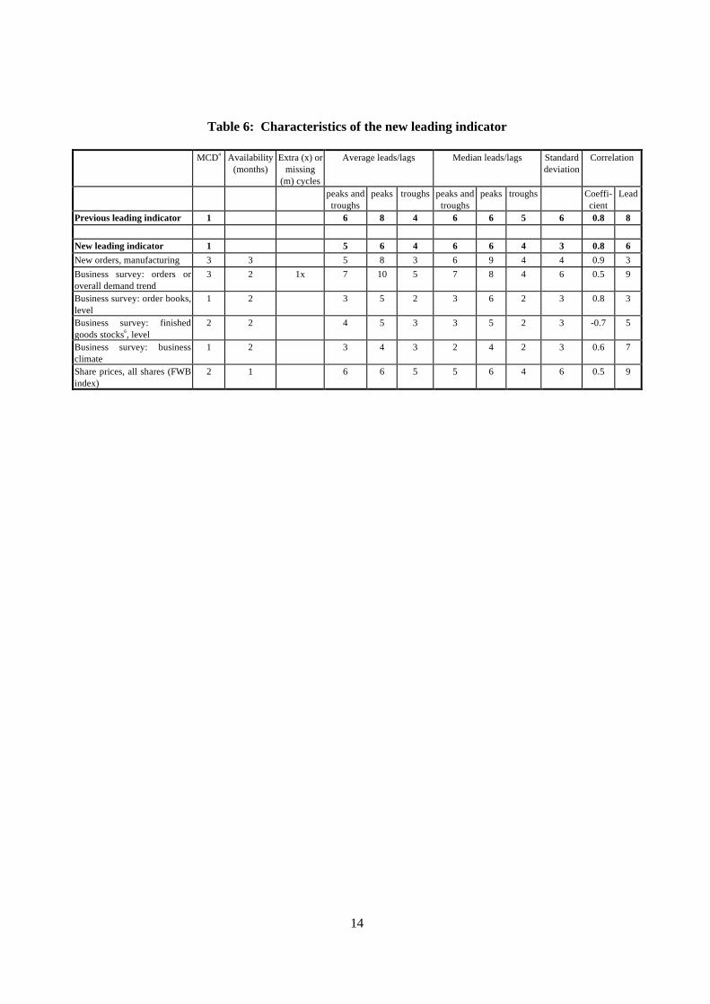
A comparison of the new indicator's performance with that of the old is summarised in Table 6. The newindicator anticipates all turning points, unlike the old one. It is also more regular in its anticipation, as isshown by the standard deviation of the lead time, which is only half as great.

14

Table 6: Characteristics of the new leading indicator

MCD4 Availability(months)

Extra (x) ormissing

(m) cycles

Average leads/lags Median leads/lags Standarddeviation

Correlation

peaks andtroughs

peaks troughs peaks andtroughs

peaks troughs Coeffi-cient

Lead

Previous leading indicator 1 6 8 4 6 6 5 6 0.8 8

New leading indicator 1 5 6 4 6 6 4 3 0.8 6

New orders, manufacturing 3 3 5 8 3 6 9 4 4 0.9 3

Business survey: orders oroverall demand trend

3 2 1x 7 10 5 7 8 4 6 0.5 9

Business survey: order books,level

1 2 3 5 2 3 6 2 3 0.8 3

Business survey: finishedgoods stocks6, level

2 2 4 5 3 3 5 2 3 -0.7 5

Business survey: businessclimate

1 2 3 4 3 2 4 2 3 0.6 7

Share prices, all shares (FWBindex)

2 1 6 6 5 5 6 4 6 0.5 9

15

NORWAY

The current leading indicator

The composite indicator for Norway, as presented in [5] (pp. 144-147), is a leading indicator ofmanufacturing production. This restriction vis-à-vis aggregate industrial output stems from the volume ofcrude oil production, whose cyclical profile is not comparable to that of the reference series. It must bestressed that the reference series is highly volatile, as indicated by its Months for Cyclical Dominance orMCD11 value of 6. This is due to the fact that Norwegian production is quite specialised (in particular,chemicals and wood).

Initially the composite leading indicator was made up of eleven series:

1. Industrial production, export goods;2. Stocks of domestic goods;3. Stocks of export goods;4. Stocks of imported goods (volume);5. Crude materials stocks;6. Production tendency;7. Inflow of export orders, tendency;8. Business outlook;9. Share prices, industrials, Oslo Stock Exchange;10. Construction costs, dwellings;11. Value of export goods, excluding ships.

Out of these eleven series, seven are quarterly (series 2-8). Series 6-8 are net percentages of the balance of“positive” over “negative” obtained from the quarterly business survey. Initially, the indicator's medianlead (peaks and troughs) was four months, with an average lead of three months and a standard deviationof 3.9 months. The maximum correlation with the reference series was 0.84 at a six-month lead.

Since the leading indicator was established, Statistics Norway has stopped calculating stock data, andseries 2-5 have not been updated since the third quarter of 1990. The first component (industrialproduction, export goods) has not been updated since January 1992. None of these series have beenreplaced. It must also be pointed out that, over the period available the cycles of construction costs (10)and the value of export goods (11) no longer correspond to those of the reference series since 1986 and1982 respectively.

For this reason, since 1992 the indicator has been computed using only six of the eleven components; ofthese six, three (series 6-8) are quarterly.

On average, it now takes about three months to obtain monthly data, just as it generally does for quarterlyseries from business surveys. However, at the time of writing (June 1996), the most recent data availablewere from fourth-quarter 199512.

16

Updates of the composite indicator are entirely dependent on the quarterly data, and five of its componentsare no longer up-to-date. For this reason, on average it comes out substantially later than most of the otherleading indicators computed by the OECD, which are updated an average of three months after thereference period.

When quarterly data become available, data for the composite indicator are updated for three consecutivemonths. The time lag between the reference period and publication therefore varies between four months,as it was initially, and six months, when there are no updates of quarterly data.

Clearly, then, the quality of the leading indicator for Norway has deteriorated. As it happens, thechronology of turning points for 1983-90 does not correspond to that of the reference series: the referenceseries' major peak in June 1986 is missing, and the December 1991 trough is not anticipated. Themaximum correlation with the reference series is currently 0.60 at a five-month lead.

The new indicator

After consultations with the Norway country desk, it was decided to maintain the reference series(manufacturing production) despite its volatility, the exclusion of oil production being deemed justified.Later we shall have more to say about the relevance of the choice of a reference series. Cycles of thereference series that were detected at the time of the initial calculation were confirmed, and cycles after1986 were updated.

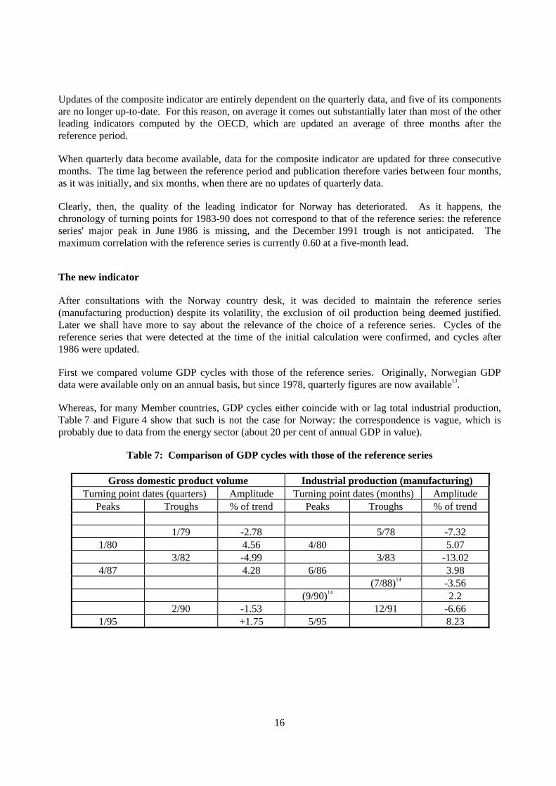
First we compared volume GDP cycles with those of the reference series. Originally, Norwegian GDPdata were available only on an annual basis, but since 1978, quarterly figures are now available13.

Whereas, for many Member countries, GDP cycles either coincide with or lag total industrial production,Table 7 and Figure 4 show that such is not the case for Norway: the correspondence is vague, which isprobably due to data from the energy sector (about 20 per cent of annual GDP in value).

Table 7: Comparison of GDP cycles with those of the reference series

Gross domestic product volume Industrial production (manufacturing)Turning point dates (quarters) Amplitude Turning point dates (months) Amplitude

Peaks Troughs % of trend Peaks Troughs % of trend

1/79 -2.78 5/78 -7.321/80 4.56 4/80 5.07

3/82 -4.99 3/83 -13.024/87 4.28 6/86 3.98

(7/88)14 -3.56(9/90)14 2.2

2/90 -1.53 12/91 -6.661/95 +1.75 5/95 8.23

17

Figure 4: Ratio to trend for GDP4 and the reference series4

Jan-78 Jan-79 Jan-80 Jan-81 Jan-82 Jan-83 Jan-84 Jan-85 Jan-86 Jan-87 Jan-88 Jan-89 Jan-90 Jan-91 Jan-92 Jan-93 Jan-94 Jan-950.9

0.95

1

1.05

1.1

Ratio to trend

Reference Volume GDP

We have been looking for new components with a cyclical profile that anticipates that of the referenceseries. It should first be pointed out that, at the time of the study (May-June 1996), access to StatisticsNorway's data was limited and that a procedure for weekly Internet transfers of the data used by the MainEconomic Indicators Division was in preparation.

Examination of the current up-to-date components confirmed the cyclical pertinence of the three quarterlybusiness survey series, and that of share prices, with the updated list of reference series turning points.

Two new series were successfully tested: an international basket of long-term (ten-year) interest rates15,with the co-operation of the Bank of Norway, and the OECD's leading indicator for Sweden, which stillperforms satisfactorily. A number of trials on variables dealing with the “real” economy (in particular,total exports, components of industrial production, prices, production and exports of crude oil, in terms oflevels or monthly changes) proved unsuccessful.

Virtually all series tested yielded cycles that did not fit exactly with the reference series after the 1986peak, which was also suggested by the Norway country desk16. Each time, there were extra cycles notpresent in the reference series, in particular between 1983 and 1985 but also in 1987. The composite thatwas ultimately selected presents two extra phases (peak January 1984 - trough March 1985; troughJanuary 1987 - peak September 1987), respectively present in four and two of the six chosen components.

The indicator does not miss any cycle present in the reference series. It announces the recovery that beganin 1992 (trough in December 1991), the brief reversal in mid-1995, and it would appear to announce therecovery that was observed thereafter.

It is made up of the following six series and is presented in Table 8:

1. International basket of interest rates;2. Share prices, industrials (Oslo stock exchange);3. OECD leading indicator for Sweden;4. Business outlook;5. Production tendency;6. Inflow of export orders, tendency.

18

Table 8: Characteristics of the new leading indicator

MCD4 Availability(months)

Extra (x) ormissing (m)

cycles

Startdate

Average leads/lags Median leads/lags Standarddeviation

Correlation

peaks andtroughs

peaks troughs peaks andtroughs

peaks troughs Coeffi-cient

Lead

Previous leadingindicator

1 5 1x,1m 1/71 4.4 6.8 1.3 6 6.5 5 6.11 0.60 5

New leading indicator 2 3 2x 6/74 7.2 9.6 4.3 6 11 6 4.74 0.71 7

International basket of

interest rates61 2 1x,1m 1/78 12.8 9 16.5 15.5 9 16.5 7.27 -0.73 18

Share prices 2 2 2x 1/71 4 7 1 3.5 6 1.5 6.24 0.62 5

OECD leadingindicator for Sweden

1 3 1x,1m 1/72 10.3 12.8 7.3 10 13 6 4.80 0.76 8

Business outlook 1Q 3 2x 74Q02 3.8 4.8 2.8 7 8 3 7.80 0.62 6

Production tendency 2Q 3 1x 74Q02 3.5 4.8 2.2 4.5 5 1 3.95 0.58 6

Inflows of exportorders, tendency

1Q 3 3x 74Q02 9.2 10.2 8.2 7 11 7 5.37 0.51 6

Figure 5: Leading indicator7 and reference series4, ratio to trend

Jan-75 Jan-76 Jan-77 Jan-78 Jan-79 Jan-80 Jan-81 Jan-82 Jan-83 Jan-84 Jan-85 Jan-86 Jan-87 Jan-88 Jan-89 Jan-90 Jan-91 Jan-92 Jan-93 Jan-94 Jan-950.9

0.95

1

1.05

1.1

Ratio to trend

Reference Leading Indicator

The composite indicator's MCD11 value is 2, which underscores its volatility. It is just as dependent onupdates of its quarterly components as the previous indicator.

The correlation at a seven-month lead between the composite indicator and the reference series is 0.71 forthe whole period. Except for the extra cycles, the new indicator's chronology of turning points fits wellwith the cycles of the reference series. Moreover, its overall performance is better than that of the currentindicator, recalculated to reflect cycles after 1986:

• The fact that the standard deviation of the new indicator's lead time (4.74) is lower than that of thepresent indicator (6.11) shows greater regularity in the anticipation of turning points.

• The new indicator anticipates the major peak of June 1986 (Table 7).• The new indicator's lead is uniformly greater than that of the old one, over the entire period, and is

more pronounced after 1990: the latest trough, in December 1991, is anticipated five months inadvance, whereas the current indicator fails to detect it in time. The latest peak, in May 1995, isanticipated 13 months in advance, versus seven for the current indicator.

19

The presence of extra cycles in the six composite series may call the reference series into question.Moreover, this series is a volatile one, as stated above. Is industrial production the best choice forascertaining the business cycle? This issue for debate casts doubt on a past decision of the Secretariat toadopt a single reference series, industrial production, whenever such a series exists.

Figure 6: Current7 and new indicators7, comparison with the reference series4, ratio to trend

Jan-75 Jan-76 Jan-77 Jan-78 Jan-79 Jan-80 Jan-81 Jan-82 Jan-83 Jan-84 Jan-85 Jan-86 Jan-87 Jan-88 Jan-89 Jan-90 Jan-91 Jan-92 Jan-93 Jan-94 Jan-950.9

0.95

1

1.05

1.1Ratio to trend

Référence Ancien indicaé nouvel iReference Current Leading Indicator New Leading Indicator

20

CONCLUSIONS

The four examples studied above suggest a number of conclusions as to how the quality of componentshas evolved over time. It would appear that monetary series (United States, Germany) no longer anticipatethe business cycles of the 1980s and 90s correctly. The use of interest rates yields results of variablequality (adequate for Mexico and Norway over the entire period, mediocre for the United States andGermany). In contrast, surveys of business prospects remain accurate tools for anticipating businesscycles.

In addition, the study of Norway illustrates how the choice of a reference series can be a problem forascertaining cycles. The same problem arises on a more general level for all countries. The leadingindicator for the United States, which remains subject to substantial “noise”, illustrates the problem ofsmoothing the composite indicator.

These conclusions could apply across the board for any revision of the leading indicators of othercountries, which might take place in 1997 if the Statistics Directorate's resources permit. They are nowsubmitted to members of the working party for their comments.

21

NOTES

1. Since late 1981, a set of charts (ratio to trend and trend restored) had already been published forthree areas (OECD-Total, OECD-Europe and North America) and for Japan.

2. One of the top priorities is to update information about the data (“metadata”) published in MainEconomic Indicators, the importance of which was voiced during the meeting for thepublication’s thirtieth anniversary in October 1995.

3. New methodology based on the 1993 SNA and wider coverage of the manufacturing sector,beginning in 1993. Historical data for years prior to 1993 were reconstructed using ratiosbetween the old and the new data in 1993.

4. A series smoothed by an MCD (Months for Cyclical Dominance) moving average. See alsoNote No. 11.

5. Securities indexed to the US dollar.

6. Inverse relationship.

7. Adjusted to fit the amplitudes of the reference series.

8. The SINIEE database was not available on diskette until March 1996.

9. For further information on the sources and definitions of these series, see Main EconomicIndicators: Sources and Definitions, OECD, May 1996.

10. Unified Germany after 1991.

11. See [5], pp. 38, 42 and 75.

12. Data are taken from Statistics Norway’s weekly publication Ukens statistikk.

13. The chronological series used for GDP is taken from the Analytical DataBase (ADB), which ismanaged by the OECD Economics Department.

14. The phase between July 1988 and September 1990, of low amplitude and short duration, wasdeemed minor and appears in parentheses.

15. Weighted average long-term interest rates of Norway’s nine leading trade partners: Germany,Sweden, United Kingdom, United States, France, Denmark, Japan, the Netherlands and Canada.

16. Drop in oil prices in 1986. See [7] p. 70.

22

REFERENCES

[1] ARTIS, M.J., R.C. BLADEN-HOWELL and W. ZHANG (1995), “Turning Points in theInternational Business Cycle: An Analysis of the OECD Leading Indicators for the G-7Countries”, OECD Economic Studies, No. 24, first quarter.

[2] DURAND, Martine, Jacques SIMON and Colin WEBB (1992), “OECD’s Indicators ofInternational Trade and Competitiveness”, OECD Economics Department Working Papers, No.120.

[3] INEGI (1992), Sistema de Indicadores Adelantados para la Economía Mexicana.

[4] NILSSON, Ronny (1987), “OECD Leading Indicators”, OECD Economic Studies, No. 9,Autumn.

[5] OECD (1987), OECD Leading Indicators and Business Cycles in Member Countries 1960-1985:Sources and Methods, No. 39, January.

[6] OECD (1995), OECD Economic Surveys. Mexico, September.

[7] OECD (1995), OECD Economic Surveys. Norway, August.