arX

iv:c

ond-

mat

/030

9309

v1 [

cond

-mat

.str

-el]

12

Sep

2003

Ground state features of the Frohlich model

G. De Filippis, V. Cataudella, V. Marigliano Ramaglia, C.A. Perroni, and D. Bercioux

Coherentia-INFM and Dipartimento di Scienze Fisiche,

Universita degli Studi di Napoli “Federico II”,

Complesso Universitario Monte Sant’Angelo,

Via Cintia, I-80126 Napoli, Italy

(October 22, 2018)

Following the ideas behind the Feynman approach, a variational wave

function is proposed for the Frohlich model. It is shown that it provides,

for any value of the electron-phonon coupling constant, an estimate of the

polaron ground state energy better than the Feynman method based on path

integrals. The mean number of phonons, the average electronic kinetic and

interaction energies, the ground state spectral weight and the electron-lattice

correlation function are calculated and successfully compared with the best

available results.

1

I. INTRODUCTION

In recent years a large amount of experimental results has pointed out that the electron-

phonon (e-ph) interaction plays a significant role in determining the electronic and mag-

netic properties of new materials as the high Tc superconductors and the colossal magneto-

resistance manganites.1 The experimental data have given rise to a renewed interest in

models of the e-ph coupled system. In this paper we investigate the polaronic features of

the Frohlich model within a variational approach.2 Here the picture is the following. When

an electron in the conduction band of a polar crystal moves through the crystal, its Coulomb

field produces in its neighborhood an ionic polarization that will influence the electron mo-

tion. Then the particle must carry this polarization with it during its motion through the

crystal. The quasi-particle formed by the electron and the induced polarization charge is

called polaron. Within the Frohlich model: 1) the optical modes have the same frequency;

2) the dielectric is treated as a continuum medium; 3) in the undistorted lattice the electron

moves as a free particle with a quadratic dispersion relation (effective band mass approxi-

mation).

The problem of finding the ground state energy of the Frohlich Hamiltonian attracted

the interest of a lot of researchers mainly in the period 1950-1955. Numerous mathemati-

cal techniques have been used to solve this problem: from the perturbation theory in the

weak coupling regime3 to the strong coupling theory,4 from the linked cluster theory5 to

variational6 and Monte Carlo approaches.7,8 The weak coupling regime is well described

within the Lee, Low and Pines (LLP) approach.9 Here, after the dependence of the Hamil-

tonian on the electron coordinates has been eliminated, an upper bound for the polaron

ground state energy is obtained by using a variational wave function which is based on the

physical assumption that successive virtual phonons are emitted independently. In the op-

posite regime, when the e-ph interaction is very strong, a good description of the polaron

features has been obtained by Landau and Pekar.10 Their theory, based on a variational

calculation, stems from the idea that, for very large values of the e-ph coupling constant,

2

the electron can follow adiabatically the quantum zero-point fluctuations of the polarization

field. In their first papers the electron is localized with a Gaussian wave function. Next,

the method has been improved by Hohler11 by constructing an eigenstate of the total wave

number by superposing Landau-Pekar states localized at different points of the lattice. In

any case the validity of LLP and Hohler approaches is restricted, respectively, to weak and

strong e-ph coupling regimes.

An excellent approximation, that is accurate at all couplings, has been introduced by

Feynman.12 His approach provides a variational estimate of the electron self-energy based

on the path integrals and the Feynman-Jensen inequality. After the phonon variables have

been eliminated exactly, Feynman introduces a model Hamiltonian which describes approx-

imatively the interaction of the electron with the lattice. This Hamiltonian is that of an

electron coupled to another particle with a harmonic oscillator coupling. The trial action for

the system is obtained by eliminating the coordinates of the fictitious particle simulating the

phonon degrees of freedom. The mass M of the fictitious particle and the spring constant

are the two variational parameters within the Feynman approach. The Monte Carlo study7,8

of the Frohlich model has demonstrated the remarkable accuracy of the Feynman method

to the electron self-energy.

In this paper we use a variational technique, within an Hamiltonian approach, to investi-

gate the polaronic features of the Frohlich model. It is based on linear superposition of two

translationally invariant wave functions that provide a very good description of the weak and

strong e-ph coupling regimes. These wave functions are built assuming as starting points

the LLP9 and Hohler11 variational approaches. First, we improve these methods obtaining

a better upper bound for the polaron ground state energy in the two asymptotic regimes of

weak and strong e-ph interaction. Then, we use a linear superposition of these two wave

functions. The comparison of our results with the Feynman12 and Monte Carlo data7 shows

that the proposed method provides an excellent description of the polaron ground state

energy for any value of the e-ph coupling. Within our variational approach, the estimate of

the electron self-energy turns out systematically lower than one of the Feynman method. In

3

particular, unlike the Feynman approach, the ground state energy shows the exact depen-

dence on the e-ph coupling constant in the strong coupling regime. Next, we calculate the

mean number of phonons present in the virtual phonon cloud surrounding the electron, the

average electronic kinetic and interaction energies, the ground state spectral weight and the

induced ionic polarization charge density. These quantities are successfully compared with

Monte Carlo8 and Feynman results.13

The proposed method has the advantage to exhibit, first to the author’s knowledge,

a wave function that gives the correct behavior in both weak and strong coupling limits

and provides an interpolation between them with results at least accurate as those of the

Feynman approach.12

II. THE MODEL

The Frohlich model2 is described by the Hamiltonian:

H = Hel +Hph +He−ph =p2

2m+∑

~q

hω0a†~qa~q +

∑

~q

(Mqei~q·~ra~q + h.c.). (1)

In Eq.(1) m is the band mass of the electron, hω0 is the longitudinal optical phonon

energy, ~r and ~p are the position and momentum operators of the electron, a†~q represents

the creation operator for phonons with wave number ~q and Mq indicates the e-ph matrix

element. In the Frohlich model,2 Mq assumes the form:

Mq = ihω0

R1/2p

q

√

4πα

V, (2)

where α, dimensionless quantity, is the e-ph coupling constant, Rp =√

h2mω0

and V is the

volume of the system.

4

III. THE STRONG COUPLING REGIME

A. The adiabatic approximation

When the value of α is very large (α≫ 1) the electron can follow adiabatically the lattice

polarization changes and it becomes self-trapped in the induced polarization field. The idea

of Landau and Pekar,10 in the first works on polarons, is to use, as trial wave function for

the e-ph coupled system, a product of normalized variational wave functions |ϕ〉 and |f〉

depending, respectively, on the electron and phonon coordinates:

|ψ〉 = |ϕ〉|f〉. (3)

The expectation value of the Hamiltonian (1) on the state (3) gives:

〈ψ|H|ψ〉 = 〈ϕ| p2

2m|ϕ〉+ 〈f |

∑

~q

[

hω0a†~qa~q + ρ~qa~q + ρ∗~qa

†~q

]

|f〉 (4)

with

ρ~q =Mq〈ϕ|ei~q·~r|ϕ〉. (5)

The variational problem with respect to |f > leads to the following lowest energy phonon

state:

|f >= e

∑

~q

[

ρ~qhω0

a~q−h.c.

]

|0 > . (6)

The minimization of the corresponding energy with respect to |ϕ〉 leads to a non-linear

integro differential equation that has been solved numerically by Miyake.14 The result for

the polaron ground state energy in the strong coupling limit is:

E = −0.108513α2hω0. (7)

The Landau-Pekar10 Gaussian ansatz for |ϕ〉:

|ϕlp〉 = e−(mωh )

2 r2

2

(

mω

hπ

)3/4

, (8)

5

after the minimization of the expectation value of the Hamiltonian (1) on this state, with

respect to the variational parameter ω, provides an estimate of the ground state energy:

E = −α2

3πhω0 ≃ −0.106103α2hω0 (9)

that is very close to the exact result (7). The best value for ω turns out:

ω =4α2

9πω0. (10)

An excellent approximation for the true energy (7) is obtained by using a trial wave

function similar to that one introduced by Pekar:10

|ϕp〉 = Ne−γr[

1 + b (2γr) + c (2γr)2]

(11)

with N normalization constant and b, c and γ variational parameters. The minimization of

〈ϕp|H|ϕp〉 leads to:

E = −0.108507α2hω0. (12)

This upper bound for the energy differs from the exact value less than 0, 01%.

B. Path integral method versus Hamiltonian approach

At this point we recall the result of the Feynman12 variational calculation when the

approximating action is represented by a fixed harmonic binding potential:

E =

[

−α2

3π− 3 log 2

]

hω0, α→ ∞. (13)

It is given by the sum of two terms. The first one corresponds to use a Gaussian wave

function in the Landau and Pekar’s method (Eq.(8)). The last one does not depend on

the e-ph coupling constant α. The origin of this contribution in Feynman’s expansion of

the polaron energy has been discussed by Allcock15 by using the perturbation theory in the

strong coupling limit. Our first aim is to put this result on variational basis. This will allow

us to characterize the terms that one has to introduce in the trial wave function to improve

6

the Landau and Pekar’s ansatz. To this aim, starting from Eq.(3) and Eq. (6), we apply

the following unitary transformation:

H1 = eS1He−S1 (14)

with

S1 = −∑

~q

[

α~q

hω0a~q − h.c.

]

. (15)

The transformed Hamiltonian assumes the form:

H1 = H0 +HI (16)

with

H0 =p2

2m+∑

~q

hω0a†~qa~q −

∑

~q

[

(

Mqei~q·~r − α~q

) α∗~q

hω0

+ h.c.

]

−∑

~q

|α~q|2hω0

(17)

and

HI =∑

~q

[(

Mqei~q·~r − α~q

)

a~q + h.c.]

. (18)

One recognizes immediately that the Landau-Pekar approach corresponds to use as trial

wave function for H1:

|ψ〉(0) = |0〉|ϕlp〉 (19)

with |ϕlp〉 given by Eq.(8) and αq =Mq〈ϕlp|ei~q·~r|ϕlp〉. In other words, in this approach, one

approximates the lowest energy state of H0 with a Gaussian wave function containing the

variational parameter ω, that represents the characteristic oscillation of the electron in the

induced lattice polarization. The next order term is obtained assuming HI as perturbation

and approximating the eigenstates of H0 with those of an harmonic oscillator. At the first

order of the perturbation theory the wave function is:

|ψ〉(1) = |ψ〉(0) −∫ 1

0t[

ω0

ω−1]∑

~q

h∗~q(~r, t)a†~q|0〉|ϕlp〉dt (20)

7

where

h~q(~r, t) =Mq

hωei~q·~rte

q2

2

h2mω (t2−1) − α~q

hω. (21)

This expression has been got using the generating function of the Hermite polynomials.

Finally we note that |ψ〉(1) can be obtained from

|ψ〉 = e−S2 |ϕlp〉|0〉 (22)

with

S2 = −∫ 1

0t[

ω0

ω−1]∑

~q

[h~q(~r, t)a~q − h.c.] dt , (23)

by expanding the exponential e−S2 and truncating the expansion at the first order. Taking

into account also the unitary transformation in Eq.(14), the previous considerations lead us

to assume as trial wave function for the Frohlich Hamiltonian in the strong coupling limit:

|ψF 〉 = e−SF |ϕlp〉|0〉, (24)

with

SF = −∫ 1

0t[

ω0

ω−1]∑

~q

[

Mq

hωei~q·~rte

q2

2

h2mω (t2−1)a~q − h.c.

]

dt . (25)

We have indicated this coherent state with ”F” since it is easy to show that the expectation

value of the Frohlich Hamiltonian on the state (25) gives:

E =3

4hω − αhω0

√

ω0

ω

Γ(ω0

ω)

Γ(ω0

ω+ 1

2), (26)

i.e. the Feynman result when the approximating action is represented by a fixed harmonic

binding potential.12 In Eq.(26) Γ(x) is the Gamma function. In particular the minimization

of E with respect to the variational parameter ω and the asymptotic expansion for α → ∞

restore the Eq.(13). Then, the order beyond the Landau and Pekar’s theory is due to the

lattice fluctuations and to the consequent change in the electron wave function.

8

C. Improvements of the Feynman result

The next step is to try to improve the Feynman result. To this aim, we note that is

possible to obtain an excellent approximation of the polaron ground state energy in Eq.(26)

substituting in Eq.(25) SF with:

S = −∑

~q

[(

v~qei~q·~rη + u~qe

i~q·~r)

a~q − h.c.]

(27)

where

v~q =Mq

hω

∫ a

0t[

ω0

ω−1]e

q2

2

h2mω (t2−1) (28)

and

u~q =Mq

hω

∫ 1

at[

ω0

ω−1]e

q2

2

h2mω (t2−1) . (29)

Here a and η are two variational parameters. In other words, we obtain the main contribu-

tion to the Feynman estimate of the electron self-energy approximating SF as sum of two

terms: the first one stems from the observation that the electron moves very fast in the

induced potential well; the second one takes into account the lattice fluctuations and the

possibility that they can follow instantaneously the electron motion. In order to improve

the Feynman result, the Pekar’s approach (Eq.(11)) and the previous analysis suggest us to

try the following ansatz:

|ψ〉 = e−∑

~q[(s~qei~q·~r+l~qe

i~q·~rη)a~q−h.c.]|0〉|ϕp〉 (30)

with |ϕp〉 given by Eq.(11), η variational parameter and l~q and s~q functions to be determined

by minimizing the expectation value of the Frohlich Hamiltonian on this state. This last

quantity turns out:

〈ψ|H|ψ〉 = 〈ϕp|p2

2m|ϕp〉+

∑

~q

[

hω0

(

|l~q|2 + |s~q|2)

+h2q2

2m

(

η2|l~q|2 + |s~q|2)

]

+∑

~q

[(

hω0 +h2q2

2mη

)

(

r~qs~ql∗~q + h.c.

)

−(

Mqs∗~q +Mqr~ql

∗~q + h.c.

)

]

(31)

9

with

r~q = 〈ϕp|ei~q·~r(1−η)|ϕp〉. (32)

Making 〈ψ|H|ψ〉 stationary with respect to arbitrary variations of the functions l~q and

s~q, we obtain two, easily solvable, algebraic equations. The minimization and the asymptotic

expansion of the ground state energy, for α → ∞, provide:

E =[

−0.108507α2 − 1.89]

hω0. (33)

The electron self-energy shows the exact dependence on α2 in the strong coupling regime

together with a good estimate of the e-ph coupling constant independent contribution due to

the lattice fluctuations. This allows to obtain, for α ≥ 8.7, an upper bound for the polaron

ground state energy better than the Feynman approach when the approximating action is

represented by a fixed harmonic binding potential (Eq.(26)). On the other hand, both these

methods give the same result for α ≤ 6, i.e. E = −αhω0. However, both the methods show

a discontinuity in the transition from the weak to strong coupling regime.

To overcome this difficulty one has to take into account the translational invariance. We

construct an eigenstate of the total wave number by taking a superposition of the localized

states (30) centered on any point of the lattice in the same manner in which one constructs

a Bloch wave function from a linear combination of atomic orbitals:

|ψ(sc)〉 =∫

ψ(~r − ~R)d3R . (34)

The minimization, with respect to the variational parameters, of the expectation value of

the Frohlich Hamiltonian on this state, that accounts for the translationally symmetry, and

the asymptotic expansion for α→ ∞ provide:

E =[

−0.108507α2 − 2.67]

hω0. (35)

This upper bound is lower than the variational Feynman estimate which for large values of

α assumes the form:12

E =

[

−α2

3π− 3 log 2− 3

4

]

hω0. (36)

10

IV. THE WEAK COUPLING REGIME

When the value of α is very small the lattice follows adiabatically the electron. A good

physical description of the polaron features in this regime is provided by the LLP approach.9

The starting point is the observation that the total momentum operator:

~Pt = ~p+∑

~q

h~qa†~qa~q (37)

is a motion constant, i.e. it commutes with the Hamiltonian. The conservation law of the

total momentum is taken into account through the unitary transformation:

U = ei

(

~Q−∑

~q~qa†

~qa~q

)

·~r, (38)

where h ~Q is the eigenvalue of ~Pt. In this paper we are interested in the ground state

properties of the e-ph coupled system, so that we will restrict ourselves to the case ~Q = 0.

The transformed Hamiltonian does not contain the electron variables and it is given by:

H1 = U−1HU =∑

~q

(

hω0 +h2q2

2m

)

a†~qa~q +∑

~q

(Mqa~q + h.c.) +h2

2m

∑

~q1,~q2

~q1 · ~q2a†~q1a†~q2a~q2a~q1.

(39)

The LLP wave function is:

|ψ〉 = e∑

~q(f~qa~q−h.c.)|0〉, (40)

where |0〉 is the phonon vacuum state and f~q = Mq/(

hω0 +h2q2

2m

)

. In other words |ψ〉 is

the lowest energy state of the first two terms of the transformed Hamiltonian H1. The use

of this wave function is based on the physical assumption that, when the e-ph interaction

is weak, there is not correlation among the emission of successive virtual phonons by the

electron. This assumption restricts the validity of this approach to the regime characterized

by small values of α. The ground state energy turns out E = −αhω0. In other words, this

method puts the results of the perturbation theory on variational basis.

To improve the LLP approximation,9 one has to introduce in the trial wave function a

better description of the recoil effect of the electron, effect present only on average in LLP

approach. This can be done using the following ansatz:

11

|ψ(wc)〉 = e∑

~q(g~qa~q−h.c.)

|0〉+∑

~q1,~q2

d~q1,~q2a†~q1a†~q2|0〉

, (41)

that takes into account the correlation between the virtual emission of pairs of phonons.16

In this paper we will choose:

g~q =Mq

(

hω0 +h2q2

2mǫ2) (42)

and

d~q1,~q2 = γhω0h2

2m~q1 · ~q2

Mq1(

hω0 +h2q2

1

2mδ2)

Mq2(

hω0 +h2q2

2

2mδ2) . (43)

Here γ, δ and ǫ are three variational parameters that have to be determined by minimizing

the expectation value of the Hamiltonian (1) on the state (41). This procedure provides as

upper bound for the polaron ground state energy at small values of α:

E = −αhω0 − 0.0123α2hω0, α→ 0 , (44)

i.e. the same result, at this order, of the Feynman approach.12 We stress that, at the α2

order, the result for the electron self-energy is:

E = −αhω0 − 0.0159α2hω0 (45)

as found by Hohler and Mullensiefen,17 Larsen16 and Roseler.18

V. ALL COUPLINGS

A careful inspection of the wave function (34) shows that is able to interpolate between

strong and weak coupling regimes. On the other hand, for small values of α a better

description of the polaron ground state features is provided by the wave function (41).

Moreover, in the weak and intermediate e-ph coupling, α ≤ 7, these two solutions are not

orthogonal and have non zero off diagonal matrix elements. This suggests that the lowest

state of the system is made of a mixture of the two wave functions that give an accurate

12

description of weak and strong e-ph coupling regimes. Then the idea is to use a variational

method to determine the ground state energy of the Hamiltonian (1) by considering as trial

state a linear superposition of the two previously discussed wave functions:

|ψ〉 =A|ψ(wc)〉+B|ψ(sc)〉√A2 +B2 + 2ABS

, (46)

where

|ψ(wc)〉 =|ψ(wc)〉

√

〈ψ(wc)|ψ(wc)〉, |ψ(sc)〉 =

|ψ(sc)〉√

〈ψ(sc)|ψ(sc)〉, (47)

and S is the overlap factor:

S =〈ψ(wc)|ψ(sc)〉+ h.c.

2. (48)

In Eq.(46) A and B are two additional variational parameters that provide the relative

weight of the two solutions in the ground state of the system. In this paper we perform

the minimization procedure in two steps. First, the expectation values of the Frohlich

Hamiltonian on the two trial wave functions in Eq.(41) and Eq.(34) are minimized and the

variational parameters are determined. Then, the minimization procedure discussed in the

present section is carried out. This way to proceed simplifies significantly the computational

effort and makes all described calculations accessible on a personal computer. An approach,

similar to that one described in this section, has been successfully used for the Holstein

model.19

The procedure of minimization of the quantity 〈ψ|H|ψ〉 with respect to A and B gives

for the polaron ground state energy

E =Em − SEc −

√

(Em − SEc)2 − (1− S2)

(

E(wc)E(sc) −E2c

)

1− S2(49)

and for the ratio of the two parameters A and B

A

B=

Ec − ES

E − E(wc)

. (50)

Here E(wc) = 〈ψ(wc)|H|ψ(wc)〉, E(sc) = 〈ψ(sc)|H|ψ(sc)〉, Em =(

E(wc) + E(sc)

)

/2 and Ec =(

〈ψ(wc)|H|ψ(sc)〉+ h.c.)

/2.

13

VI. NUMERICAL RESULTS

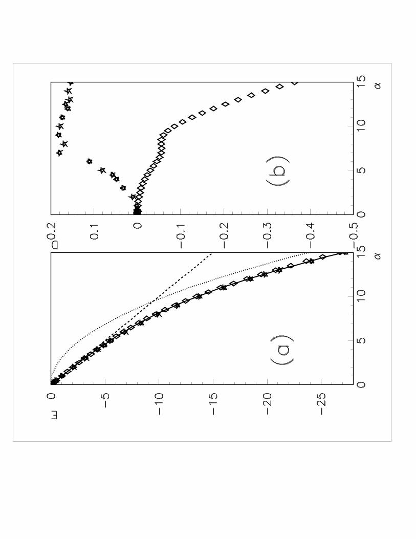
In Fig.1 we plot the polaron ground state energy, obtained within our approach, as

a function of the e-ph coupling constant α. The data are compared with the results of

the variational treatments due to Lee, Low and Pines,9 Pekar,10 Feynman12 and with the

energies calculated within a diagrammatic Quantum Monte-Carlo method.7 As it is clear

from the plots, our variational proposal recovers the asymptotic result of the Feynman

approach in the weak coupling regime, improves the Feynman’s data particularly in the

opposite regime, characterized by values of the e-ph coupling constant α ≫ 1, and it is

in very good agreement with the best available results in literature, obtained with the

Quantum Monte Carlo calculation.7 This agreement indicates that the true ground state

wave function is very close to a superposition of the above introduced functions, that provide

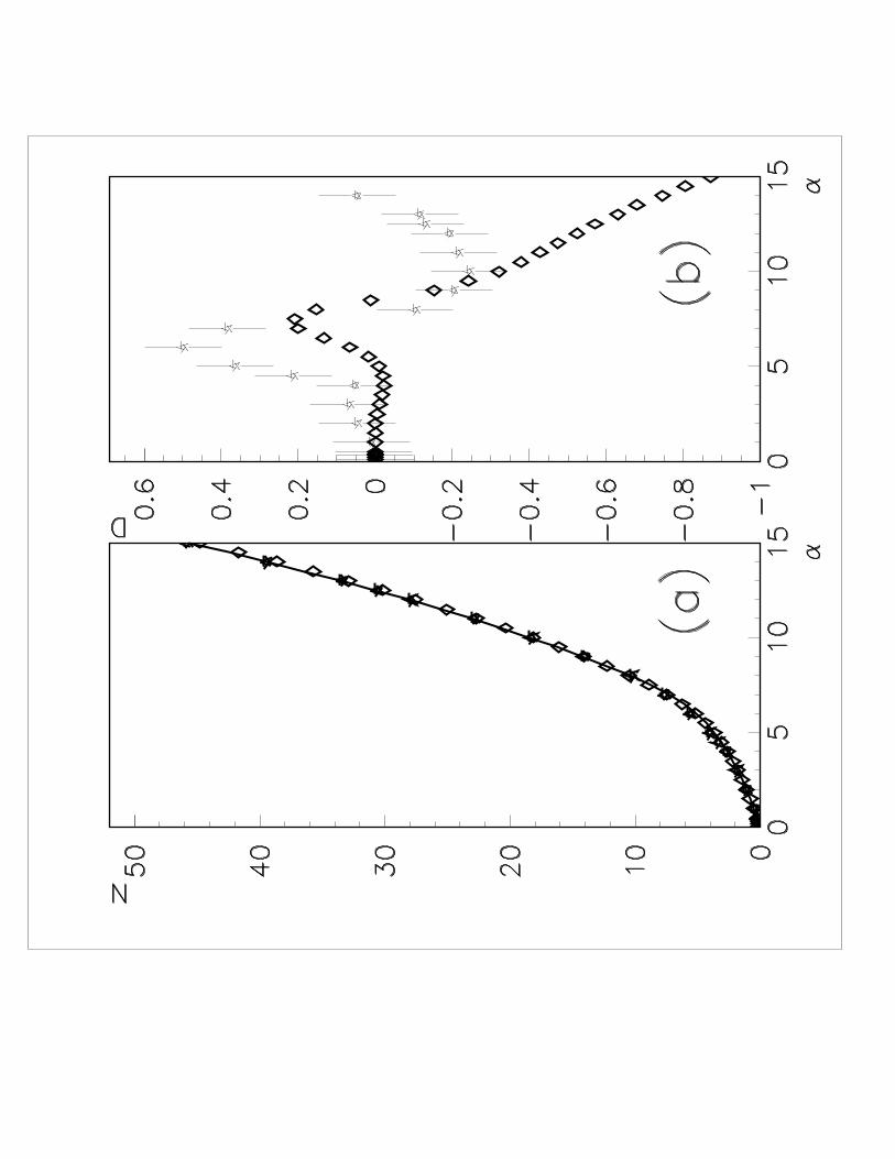
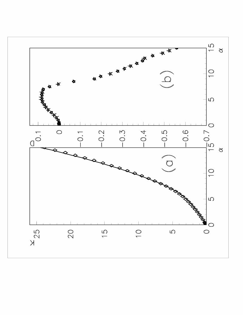
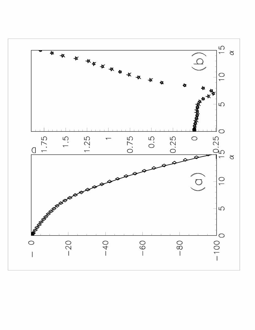
a very good description of the two asymptotic regimes. Within our approach we have also

calculated the mean number of phonons present in the virtual phonon cloud surrounding

the electron, N , the average electronic kinetic and interaction energies, K and I. These

quantities are reported, respectively, in Fig.2, Fig.3 and Fig.4 where are compared with the

same properties obtained in the Feynman’s variational treatment based on path integrals.13

As for the ground state energy, our variational ansatz is able to recover all the expected

behaviors. For small values of α, N → α/2, K → αhω0/2, I → −2αhω0 as predicted by

the LLP approach9 and the weak coupling perturbation theory.17 In the opposite regime

the electron follows adiabatically the lattice polarization changes. The values N = 2α2

3π,

K = α2

3πhω0, I = −4α2

3πhω0 obtained within the Landau and Pekar’s variational treatment

(see Eq.(8)), based on the electron self-trapping with a Gaussian wave function, represent

very accurate estimates of these quantities when they are calculated within the Feynman’s

approach. On the other hand, the values N = 2 · 0.108507α2, K = 0.108507α2hω0, I =

−4 ·0.108507α2hω0 obtained within the Pekar’s variational treatment (see Eq.(11)) represent

very good approximations for the same quantities calculated within our approach. Then the

variational Feynman’s and our methods differ mainly in the strong coupling regime as it

14

turns out from the plots in Fig.1, Fig.2, Fig.3 and Fig.4. We stress that, in this range of

values of α, our approach provides a better estimate of the polaron ground state energy than

the Feynman’s method.12

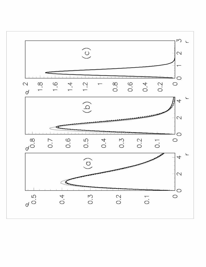
Another physical quantity of interest is ρ(~r), i.e. the average ionic polarization charge

density induced at a distance r by the electron. This quantity is related to the static

correlation function between the electron position ~re = 0 and the oscillator displacement at

~r:

ρ(~r) = −(

1

4πe

)

〈ψ(~re = 0)|∑

~q

(Mqei~q·~rq2a~q + h.c.)|ψ(~re = 0)〉. (51)

It easy to show, analytically, that the exact sum rule for the total induced charge:20

∫

ρ(~r)d3r = e(

1

ǫ∞− 1

ǫ0

)

(52)

is satisfied within our variational approach. Figure 5 shows ρ(~r)/∫

ρ(~r)d3r as a function of

r for different values of the e-ph matrix element α corresponding to weak, intermediate and

strong coupling regimes. Our data are compared with results obtained within the Feynman’s

method13 and a path integral Monte Carlo scheme.20 If the e-ph coupling is weak, the lattice

deformation is not able to trap the charge carrier. The extension of the polaron is large

compared with the characteristic length√

h2mω0

. The situation is different in the opposite

regime where the lattice deformation is localized around the electron. In any case also this

correlation function, evaluated within our approach, is in agreement with the best data

available in literature.

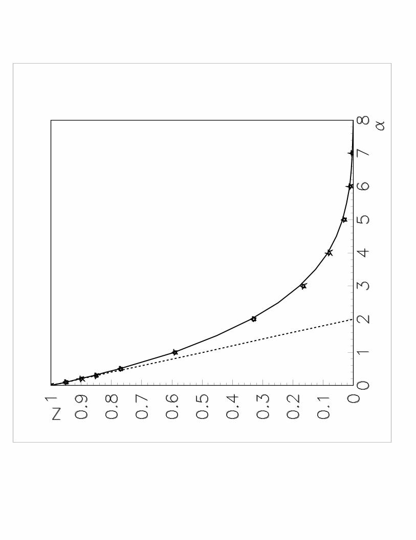
Finally Figure 6 shows the ground state spectral weight:

Z = |〈ψ|c†~k=0|0〉|2, (53)

where |0〉 is the electronic vacuum state containing no phonons and c†~k is the electron creator

operator in the momentum space. Z represents the renormalization coefficient of the one-

electron Green’s function and gives the fraction of the bare electron state in the polaron

trial wave function. This quantity is compared with that one obtained in the diagrammatic

15

Quantum Monte Carlo method.7 The result of the weak coupling perturbation theory is also

indicated: Z = 1−α/2. For small values of α the main part of the spectral weight is located

at energies that correspond approximatively to the bare electronic levels. Increasing the

e-ph interaction, the spectral weight decreases very fast and becomes practically zero in the

strong coupling regime. Here the most part of the spectral weight is located at excited states.

The diagrammatic Quantum Monte Carlo study7 of the Frohlich polaron has pointed out

that there is no stable excited states in the energy gap between the ground state energy and

the continuum. There are, instead, several many phonon unstable states at fixed energies:

Ef − E0 ≃ 1, 3.5 and 8.5hω0. These results seem to be contrary to the data about the

optical absorption of large polarons,21 which show, for large values of α, the presence of a

very narrow peak corresponding to the electronic transitions from the ground state to the

first relaxed excited state (RES). The nature of the excited states and the optical absorption

of polarons in the Frohlich model require further study which is beyond the scope of this

paper.

In conclusion, in this paper, a variational approach has been developed to investigate

the features of the Frohlich model. It has been shown that a linear superposition of two

wave functions, that describe the two asymptotic regimes of weak and strong e-ph coupling,

provides an estimate of the polaron ground state energy which is in very good agreement

with the best available results for any value of the e-ph matrix element. All the evaluated

ground state properties show that the crossover between the two asymptotic regimes is very

smooth. On the other hand the transfer of spectral weight from the polaron ground state to

the higher energy bands turns out very fast. We stress that, to the best of our knowledge, it

is the first time that a variational wave function, able to interpolate between the weak and

strong e-ph coupling regimes, at least carefully as the Feynman method,12 is exhibited for

the Frohlich model.

16

FIGURE CAPTIONS

Fig.1. (a) The polaron ground state energy, E, is reported as function of α in units of

hω0. The data (solid line), obtained within the approach discussed in this paper, are

compared with the results (diamonds) of the Feynman approach, EF , and the results

(stars) of the diagrammatic Quantum Monte-Carlo method, EMC , kindly provided by

A.S. Mishchenko. (b) The differences: E − EF (diamonds) and E − EMC (stars) are

reported as function of α.

Fig.2. (a) The mean number of phonons, N , is plotted as function of α. The data,

obtained within the approach discussed in this paper (solid line), are compared with the

results of the Feynman approach, NF (diamond), and the results of the diagrammatic

Quantum Monte-Carlo method, NMC (stars), extracted from Fig.8 of ref.7. (b) The

differences: NF − N (diamonds) and NMC −N (stars) are reported as function of α.

The error bars are due to uncertainty in the procedure used to extract the numerical

values from Fig.8.

Fig.3. (a) The average electronic kinetic energy, K, is plotted as function of α in units

of hω0. The data (solid line), obtained within the approach discussed in this paper,

are compared with the results (diamonds) of the Feynman approach, KF . (b) The

difference: KF −K (stars) is reported as function of α.

Fig.4. (a) The average electronic interaction energy, I, is plotted as function of α in units

of hω0. The data (solid line), obtained within the approach discussed in this paper,

are compared with the results (diamonds) of the Feynman approach, IF . (b) The

difference: IF − I (stars) is reported as function of α.

Fig.5. The average normalized ionic polarization charge density, induced at a distance r

by the electron, is reported for three different values of α: (a) α = 1; (b) α = 6; (c)

α = 12. The data (solid line), obtained within the approach discussed in this paper,

17

are compared with the results (dashed line) of the Feynman approach and the results

(dotted line) of the Monte-Carlo method, kindly provided by S. Ciuchi. The distance

r is measured in units of Rp.

Fig.6. The ground state spectral weight, Z, is plotted as function of α. The data (solid

line), obtained within the approach discussed in this paper, are compared with the

results (stars) of of the diagrammatic Quantum Monte-Carlo method. The result of

the weak coupling perturbation theory (dashed line) is also indicated.

1 A. Damascelli, Z. Hussain, Z.X. Shen, Rev. Mod. Phys. 75, 473 (2003); S. Lupi, P. Maselli, M.

Capizzi, P. Calvani, P. Giura, and P. Roy Phys. Rev. Lett. 83, 4852-4855 (1999); A.J. Millis,

Nature London, 392, 147 (1998).

2 H. Frohlich et al., Philos. Mag. 41, 221 (1950); H. Frohlich, in Polarons and Excitons, edited by

C.G. Kuper and G.A. Whitfield (Oliver and Boyd, Edinburg, 1963), pp. 1; for a review see: J.T.

Devreese, Polarons, in: G.L. Trigg (ed.) Encyclopedia of Applied physics, New York: VCH, vol.

14, pp. 383 (1996) and references therein.

3 G. Hohler and A.M. Mullensiefen, Z. Physik 157, 159 (1959); D.M. Larsen, Phys. Rev. 144, 697

(1966); G.D. Mahan, in Polarons in Ionic Crystals and Polar Semiconductors (North-Holland,

Amsterdam, 1972), p. 553; M.A. Smondyrev, Teor. Mat. Fiz. 68, 29 (1986).

4 L.D. Landau, Phys. Z. Sowjetunion 3, 664 (1933) [ English translation: Collected Papers (Gordon

and Breach New York, 1965), pp.67-68]; L.D. Landau and S.I. Pekar, J. Exptl. Theor. Phys.

18, 419 (1948); S.I. Pekar, Zh. Eksp. i Theor. Fiz. 19, 796 (1949); N.N. Bogoliubov and S.V.

Tiablikov, Zh. Eksp. i Theor. Fiz. 19, 256 (1949); S.I. Pekar, Research in Electron Theory of

Crystals, Moscow, Gostekhizdat (1951) [English translation: Research in Electron Theory of

Crystals, US AEC Report AEC-tr-5575 (1963)]; S.V. Tiablikov, Zh. Eksp. i Theor. Fiz. 21, 377

(1951); S.V. Tiablikov, Abhandl. Sowj. Phys. 4, 54 (1954); G.R. Allcock, Advances in Physics

18

5, 412 (1956); G. Hohler in Field Theory and the Many Body Problem, ed. E.R. Caianiello

(Accademic Press), pp.285; E.P. Solodovnikova, A.N. Tavkhelidze, O.A. Khrustalev, Teor. Mat.

Fiz. 11, 217 (1972); V.D. Lakhno and G.N. Chuev, Physics-Uspekhi 38, 273 (1995).

5 D. Dunn, Can. J. Phys. 53, 321 (1975).

6 T.D. Lee, F. Low, and D. Pines, Phys. Rev. 90, 297 (1953); M. Gurari, Phil. Mag. 44, 329 (1953);

E.P. Gross, Phys. Rev. 100, 1571 (1955); G. Hohler, Z. Physik 140, 192 (1955); G. Hohler, Z.

Physik 146, 372 (1956); R.P. Feynman, Phys. Rev. 97, 660 (1955); Y. Osaka, Prog. Theor.

Phys. 22, 437 (1959); T.D. Schultz, Phys. Rev. 116, 526 (1959); T.D. Schultz, in Polarons and

Excitons, edited by C.G. Kuper and G.A. Whitfield (Oliver and Boyd, Edinburg, 1963), pp. 71;

D.M. Larsen, Phys. Rev. 172, 967 (1968); J. Roseler, Phys. Stat. Sol. 25, 311 (1968).

7 A.S. Mishchenko, N.V. Prokof’ev, A. Sakamoto, and B. V. Svistunov, Phys. Rev. B 62, 6317

(2000); N.V. Prokof’ev and B. V. Svistunov, Phys. Rev. Lett. 81, 2514 (1998).

8 John T. Titantah, Carlo Pierleoni, and Sergio Ciuchi, Phys. Rev. Lett. 87, 206406 (2001).

9 T.D. Lee, F. Low, and D. Pines, Phys. Rev. 90, 297 (1953).

10 L.D. Landau, Phys. Z. Sowjetunion 3, 664 (1933) [ English translation: Collected Papers (Gordon

and Breach New York, 1965), pp.67-68]; L.D. Landau and S.I. Pekar, J. Exptl. Theor. Phys. 18,

419 (1948); S.I. Pekar, Research in Electron Theory of Crystals, Moscow, Gostekhizdat (1951)

[English translation: Research in Electron Theory of Crystals, US AEC Report AEC-tr-5575

(1963)].

11 G. Hohler, Z. Physik 140, 192 (1955); G. Hohler, Z. Physik 146, 372 (1956).

12 R.P. Feynman, Phys. Rev. 97, 660 (1955).

13 F.M. Peeters, and J.T. Devreese, Phys. Stat. Sol. 115, 285 (1983); F.M. Peeters, and J.T.

Devreese, Phys. Rev. B 31, 4890 (1985).

14 S.J. Miyake, J. Phys. Soc. Jap. 38, 181 (1975); S.J. Miyake, J. Phys. Soc. Jap. 41, 747 (1976).

19

15 G.R. Allcock, Advances in Physics 5, 412 (1956).

16 D.M. Larsen, Phys. Rev. 172, 967 (1968).

17 G. Hohler and A.M. Mullensiefen, Z. Physik 157, 159 (1959).

18 J. Roseler, Phys. Stat. Sol. 25, 311 (1968).

19 V. Cataudella, G. De Filippis, and G. Iadonisi, Phys. Rev. B 60, 15163 (1999); V. Cataudella,

G. De Filippis, and G. Iadonisi, Phys. Rev. B 62, 1496 (2000).

20 Sergio Ciuchi, Jose Lorenzana, and Carlo Pierleoni, Phys. Rev. B 62, 4426 (2000).

21 F.M. Peeters, and J.T. Devreese, Phys. Rev. B 28, 6051 (1983).

20