November 19th 2015

FYS4340

Summary lecture 3

Energy dispersive X-ray analysis

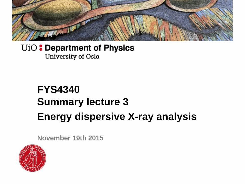
Energy dispersive X-ray spectroscopy (EDS)

• Introduction and basic physics [W&C chap. 4.1-4.2]

• Instrumentation [W&C chap. 32]

• Quantification and spectrum imaging [W&C chap. 33-35]

• Spatial resolution [W&C chap. 36]

• Fultz & Howe chapter 5.6 + 5.7

Electron beam – sample interaction

W&C

Energy transfer processes

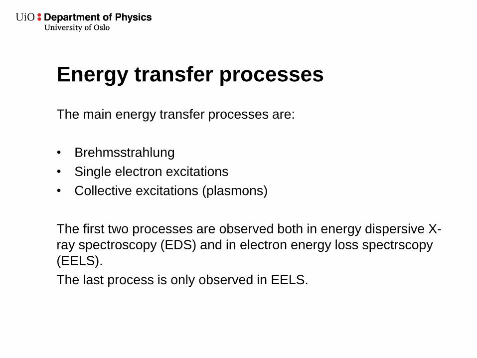
The main energy transfer processes are:

• Brehmsstrahlung

• Single electron excitations

• Collective excitations (plasmons)

The first two processes are observed both in energy dispersive X-

ray spectroscopy (EDS) and in electron energy loss spectrscopy

(EELS).

The last process is only observed in EELS.

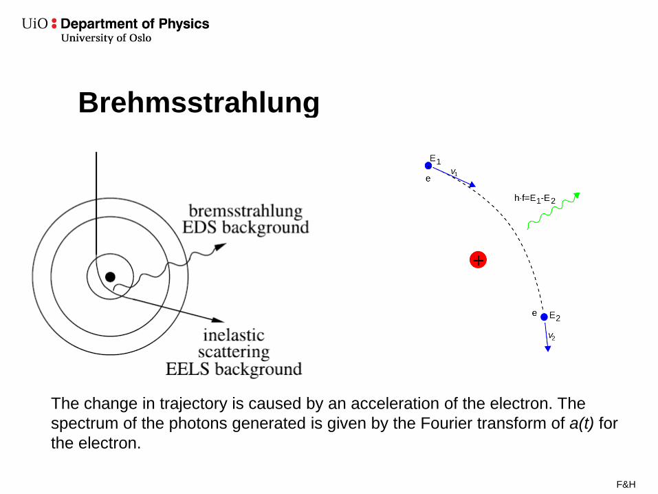
Brehmsstrahlung

The change in trajectory is caused by an acceleration of the electron. The

spectrum of the photons generated is given by the Fourier transform of a(t) for

the electron.

F&H

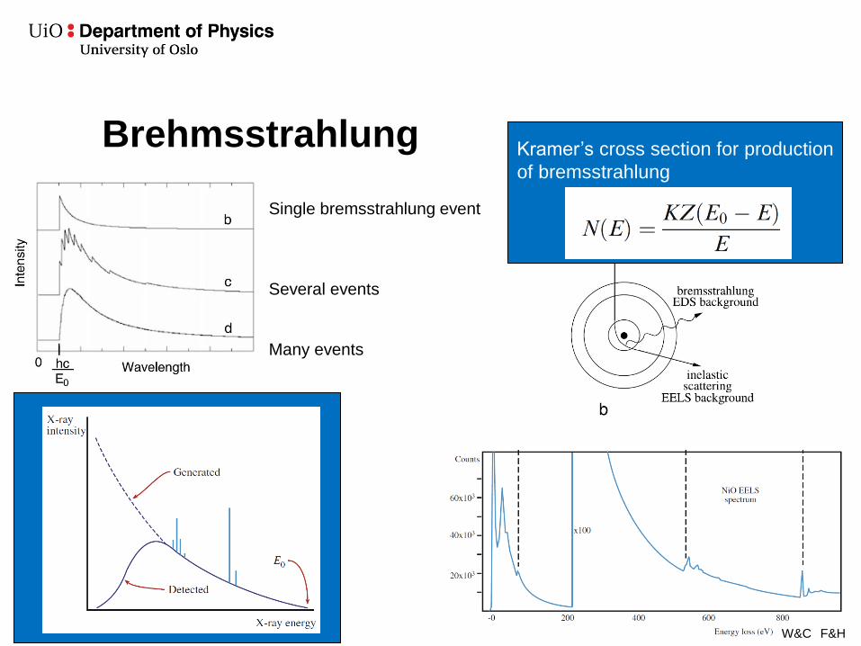
Brehmsstrahlung

Single bremsstrahlung event

Several events

Many events

Kramer’s cross section for production

of bremsstrahlung

F&H W&C

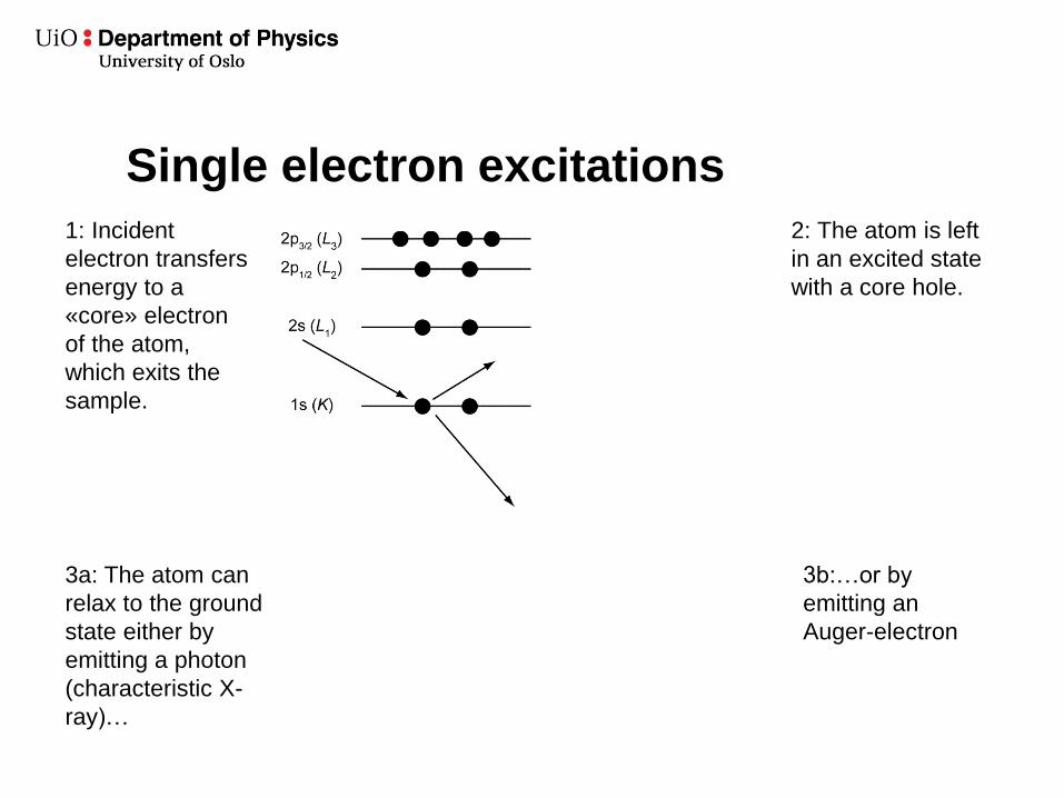
1: Incident

electron transfers

energy to a

«core» electron

of the atom,

which exits the

sample.

2: The atom is left

in an excited state

with a core hole.

3a: The atom can

relax to the ground

state either by

emitting a photon

(characteristic X-

ray)…

3b:…or by

emitting an

Auger-electron

Single electron excitations

Nomenclature

Atomic shell Main quantum

number n

Orbital quantum

number l

Total spin

quantum number

j

Spectroscopic

notation

1s 1 0 +1/2, -1/2 K

2s 2 0 +1/2, -1/2 L1

2p1/2 2 1 1/2 L2

2p3/2 2 1 3/2 L3

3s 3 0 +1/2, -1/2 M1

3p1/2 3 1 1/2 M2

3p3/2 3 1 3/2 M3

3d3/2 3 2 3/2 M4

3d5/2 3 2 5/2 M5

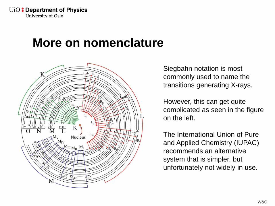
More on nomenclature

W&C

Siegbahn notation is most

commonly used to name the

transitions generating X-rays.

However, this can get quite

complicated as seen in the figure

on the left.

The International Union of Pure

and Applied Chemistry (IUPAC)

recommends an alternative

system that is simpler, but

unfortunately not widely in use.

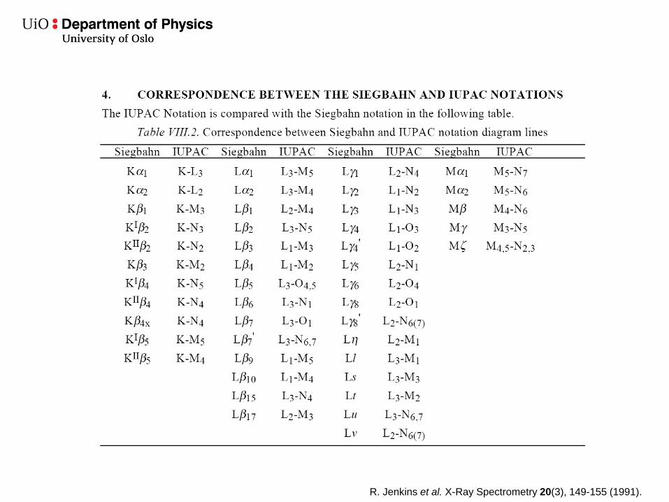
R. Jenkins et al. X-Ray Spectrometry 20(3), 149-155 (1991).

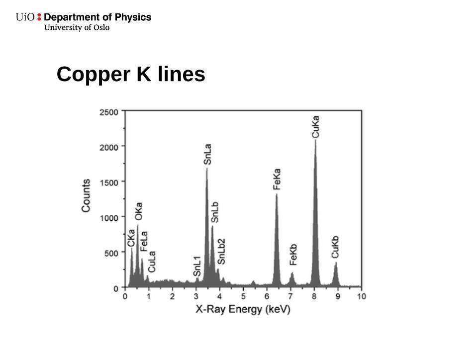
Copper K lines

Copper K lines

Eb(K) = -8979 eV

Eb(L3) = -933 eV

Eb(L2) = -952 eV

Eb(M2,3) = -76 eV

L3 -> K transition (Kα1)

E=hn= Eb(L3)- Eb(K) = 8.046 keV

L2 -> K transition (Kα2)

E=hn= Eb(L2)- Eb(K) = 8.027 keV

M2,3 -> K transition (Kb)

E=hn= Eb(M2,3)- Eb(K) = 8.903 keV

Threshold/critical energy

In order to generate X-rays, the electron beam must have an

energy E0 larger than the critical energy Ec of the process.

Usually not a problem in TEM

E0> 100 keV; Ec< 20 keV

BUT: with Cs correctors, low voltage operation has become more

common. 60 keV, 40 keV, even down to 30 keV.

For heavy elements this may limit which characteristic X-rays are

generated

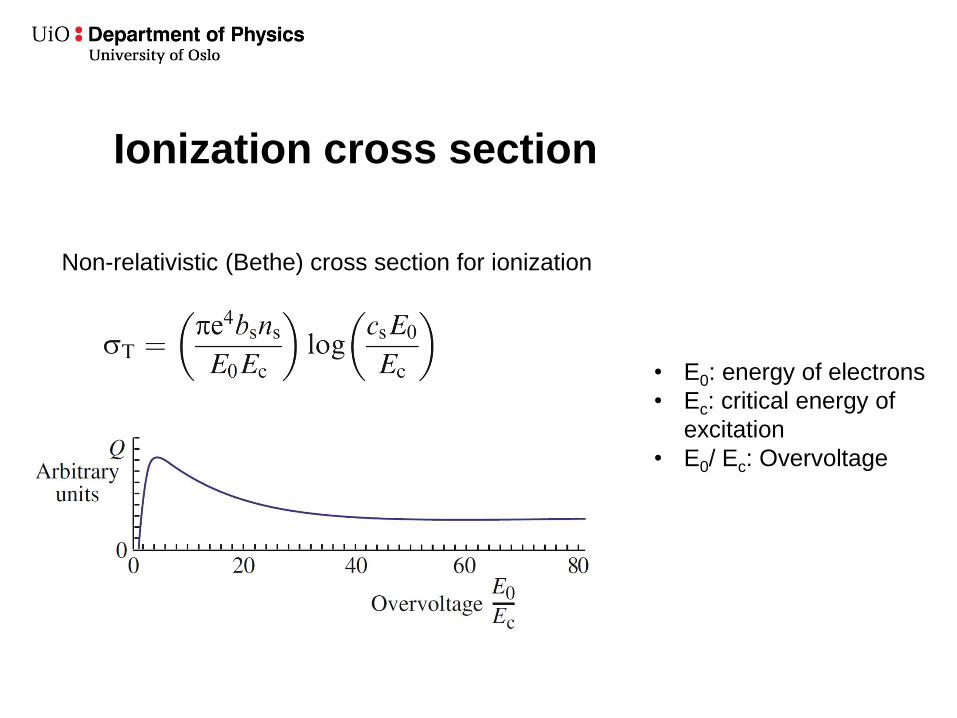
Ionization cross section

Non-relativistic (Bethe) cross section for ionization

• E0: energy of electrons

• Ec: critical energy of

excitation

• E0/ Ec: Overvoltage

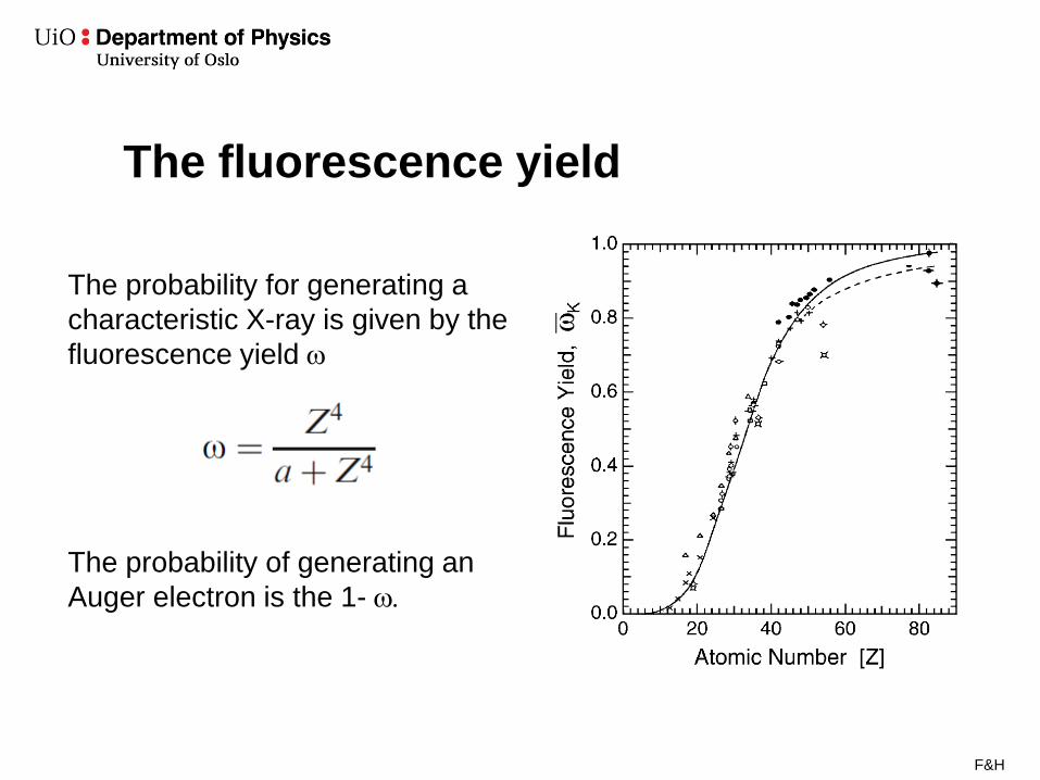
The fluorescence yield

The probability for generating a

characteristic X-ray is given by the

fluorescence yield w

The probability of generating an

Auger electron is the 1- w.

F&H

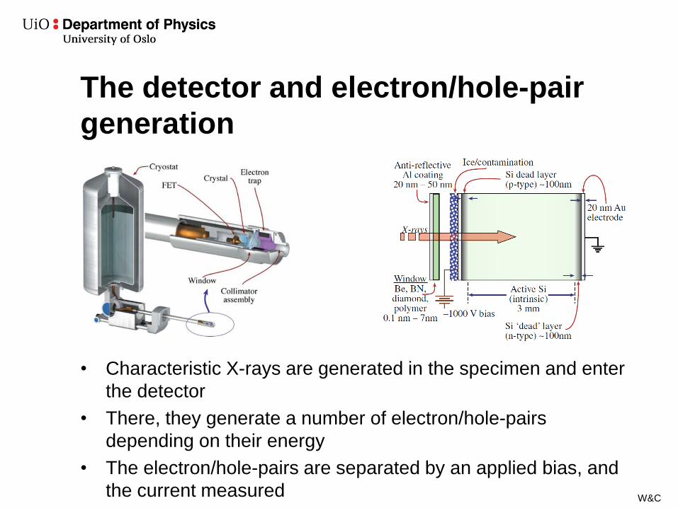
The detector and electron/hole-pair

generation

• Characteristic X-rays are generated in the specimen and enter

the detector

• There, they generate a number of electron/hole-pairs

depending on their energy

• The electron/hole-pairs are separated by an applied bias, and

the current measured W&C

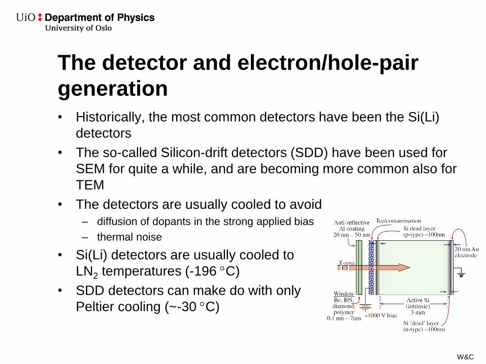
The detector and electron/hole-pair

generation

• Historically, the most common detectors have been the Si(Li)

detectors

• The so-called Silicon-drift detectors (SDD) have been used for

SEM for quite a while, and are becoming more common also for

TEM

• The detectors are usually cooled to avoid

– diffusion of dopants in the strong applied bias

– thermal noise

• Si(Li) detectors are usually cooled to

LN2 temperatures (-196 C)

• SDD detectors can make do with only

Peltier cooling (~-30 C)

W&C

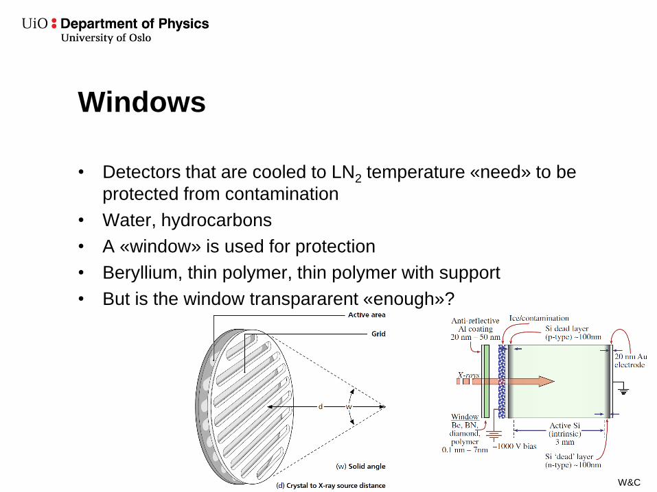
Windows

• Detectors that are cooled to LN2 temperature «need» to be

protected from contamination

• Water, hydrocarbons

• A «window» is used for protection

• Beryllium, thin polymer, thin polymer with support

• But is the window transpararent «enough»?

W&C

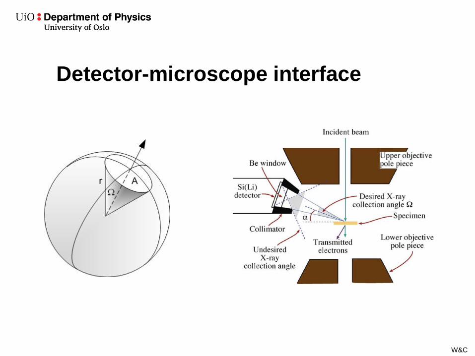
Detector-microscope interface

W&C

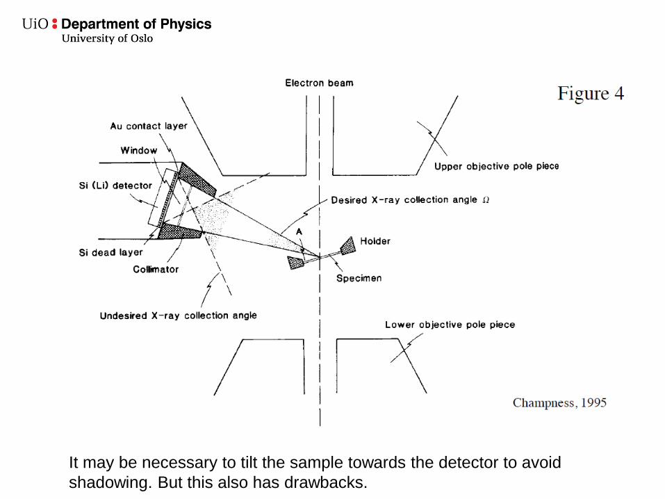
It may be necessary to tilt the sample towards the detector to avoid

shadowing. But this also has drawbacks.

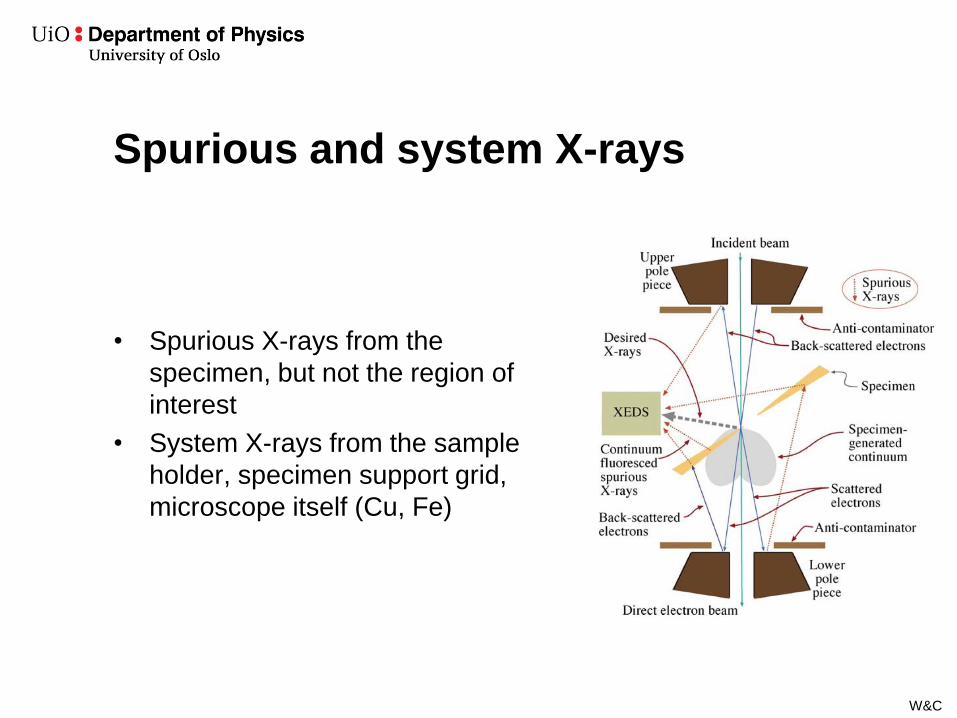
Spurious and system X-rays

• Spurious X-rays from the

specimen, but not the region of

interest

• System X-rays from the sample

holder, specimen support grid,

microscope itself (Cu, Fe)

W&C

Example: LaNbO4 doped with Sr

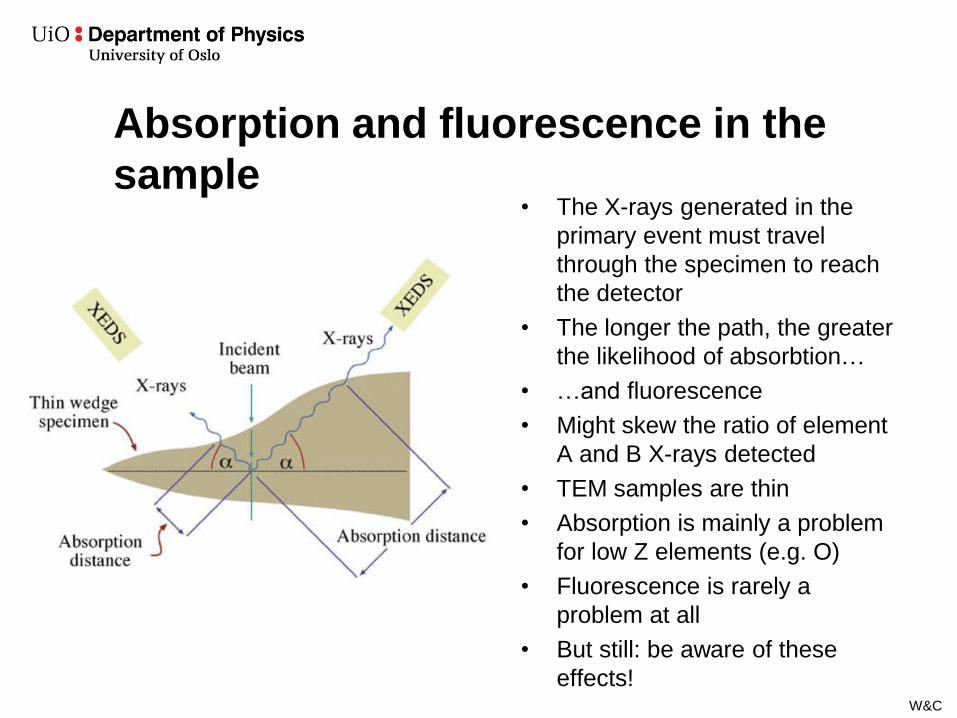
Absorption and fluorescence in the

sample • The X-rays generated in the

primary event must travel

through the specimen to reach

the detector

• The longer the path, the greater

the likelihood of absorbtion…

• …and fluorescence

• Might skew the ratio of element

A and B X-rays detected

• TEM samples are thin

• Absorption is mainly a problem

for low Z elements (e.g. O)

• Fluorescence is rarely a

problem at all

• But still: be aware of these

effects! W&C

Detector artefacts

• Escape peaks

• Internal fluorescence

• Sum peaks

• Energy resolution

Escape peaks

• The detector determines the

photon energy by measuring the

charge pulse from the electron-

hole pairs generated

• Some times, fluorescence occurs

in the detector, and a Si K

photon is generated

• This photon can leave the

detector, taking with it some of the

energy that «should» have gone

into making electron-hole pairs

• The detector then sees a smaller

charge pulse, which is interpreted

as a lower energy of the incoming

photon giving a peak at E-1.74

keV

• Usually a small effect, but be

aware when counting for a long

time

W&C

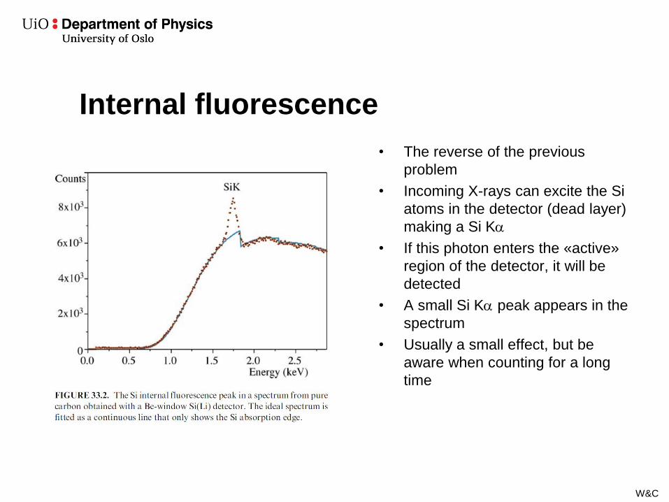
Internal fluorescence

• The reverse of the previous

problem

• Incoming X-rays can excite the Si

atoms in the detector (dead layer)

making a Si K

• If this photon enters the «active»

region of the detector, it will be

detected

• A small Si K peak appears in the

spectrum

• Usually a small effect, but be

aware when counting for a long

time

W&C

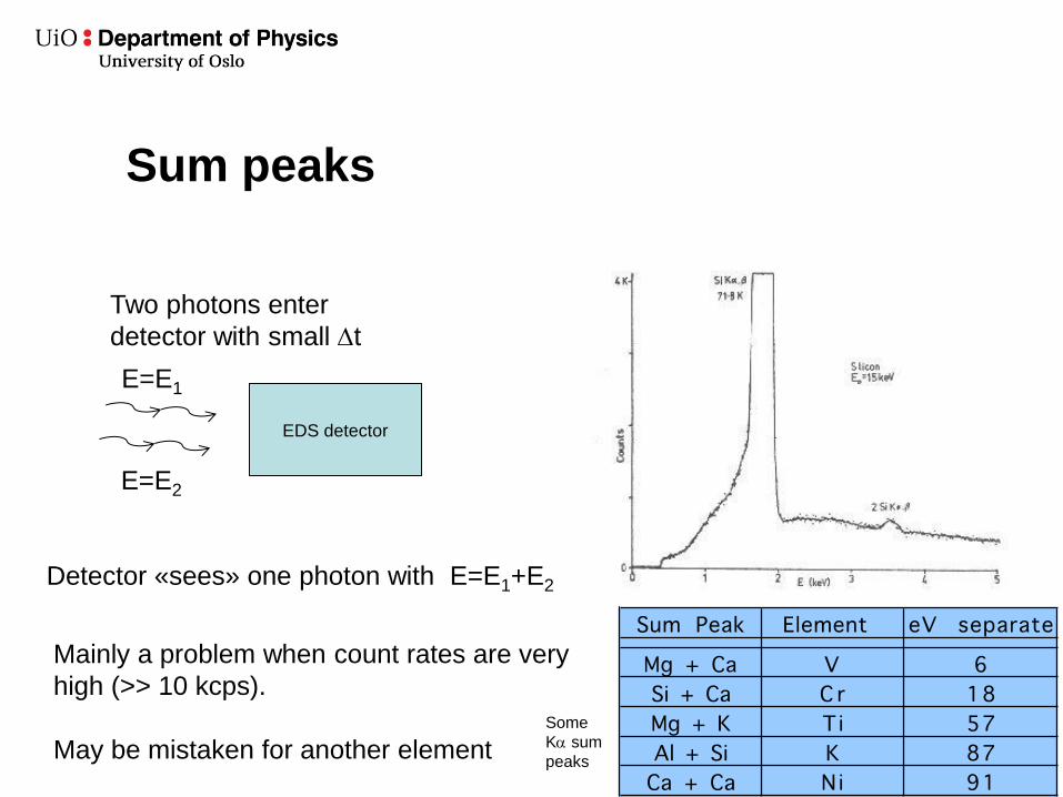
Sum peaks

Detector «sees» one photon with E=E1+E2

E=E1

E=E2

EDS detector

Two photons enter

detector with small t

Mainly a problem when count rates are very

high (>> 10 kcps).

May be mistaken for another element Some

K sum

peaks

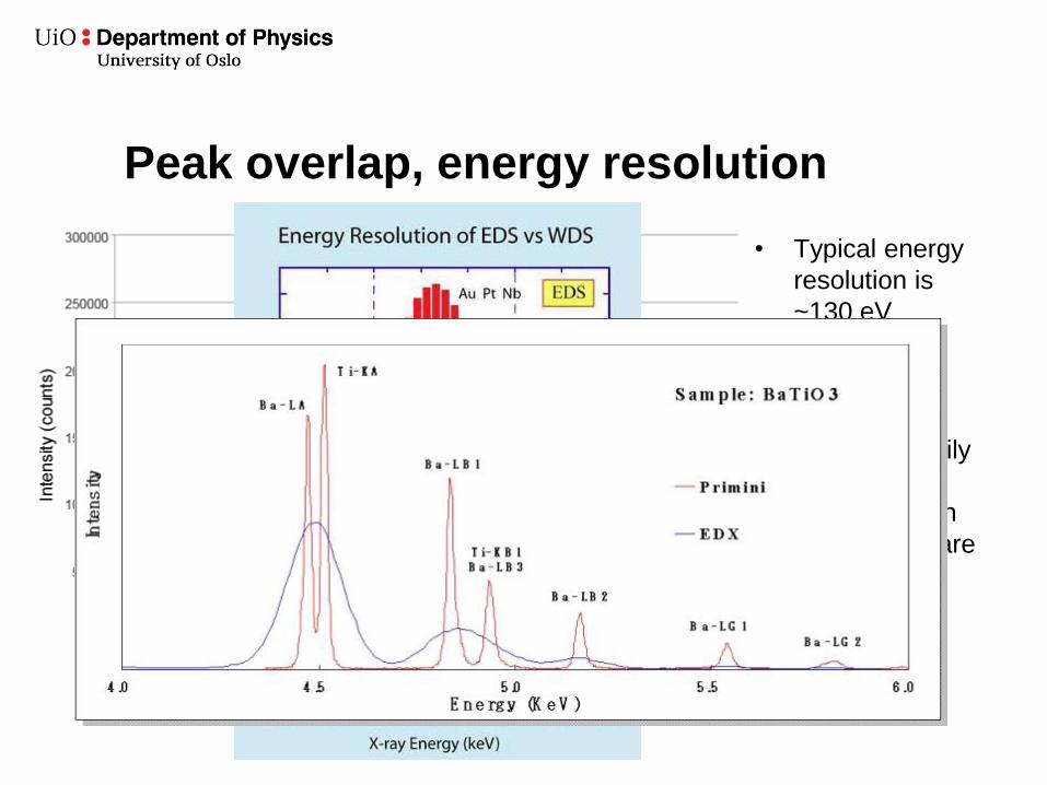
Peak overlap, energy resolution

• Typical energy

resolution is

~130 eV

• Measured as

FWHM of Mn

K

• You may easily

see only one

peak where in

reality there are

many

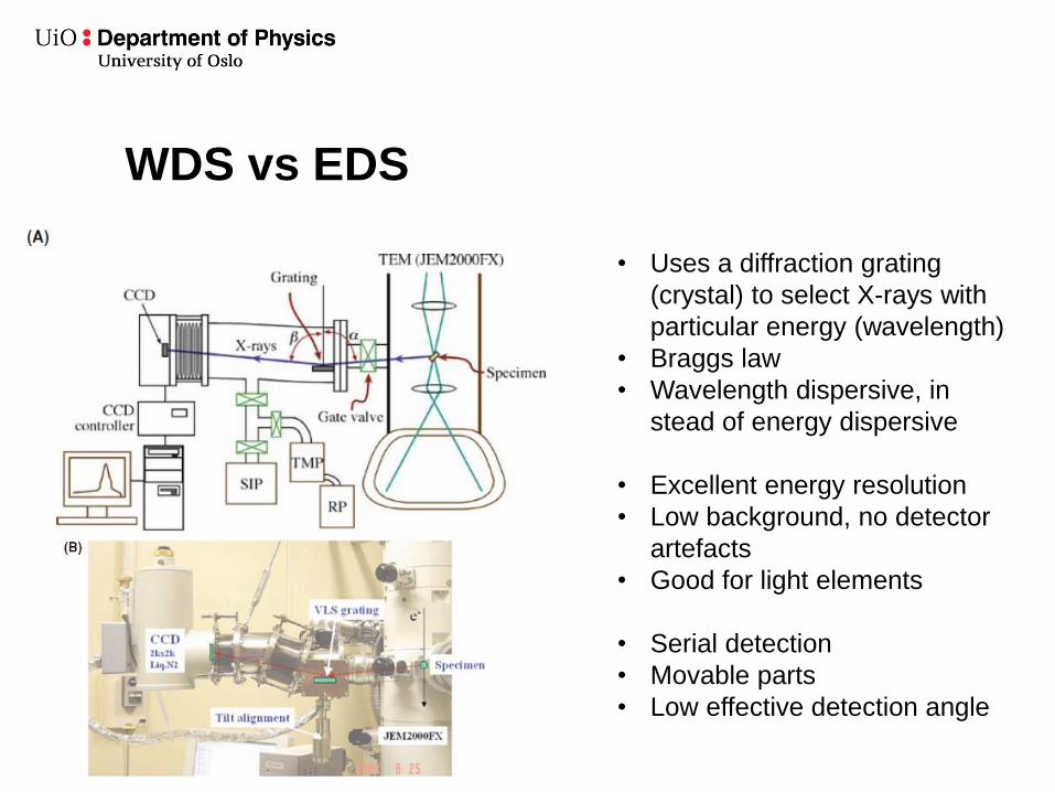
WDS vs EDS

• Uses a diffraction grating

(crystal) to select X-rays with

particular energy (wavelength)

• Braggs law

• Wavelength dispersive, in

stead of energy dispersive

• Excellent energy resolution

• Low background, no detector

artefacts

• Good for light elements

• Serial detection

• Movable parts

• Low effective detection angle

Quantification from EDS spectra

• How to get from a spectrum to composition

• Assumptions usually made in EDS in TEM

• Cliff-Lorimer k-factor method

• Limits of the CL-method and the assumptions

made

• Statistical errors

Williams & Carter chapter 35

30

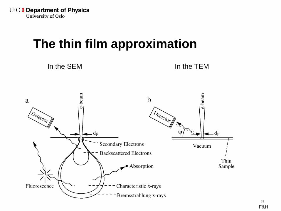
The thin film approximation

F&H

In the SEM In the TEM

31

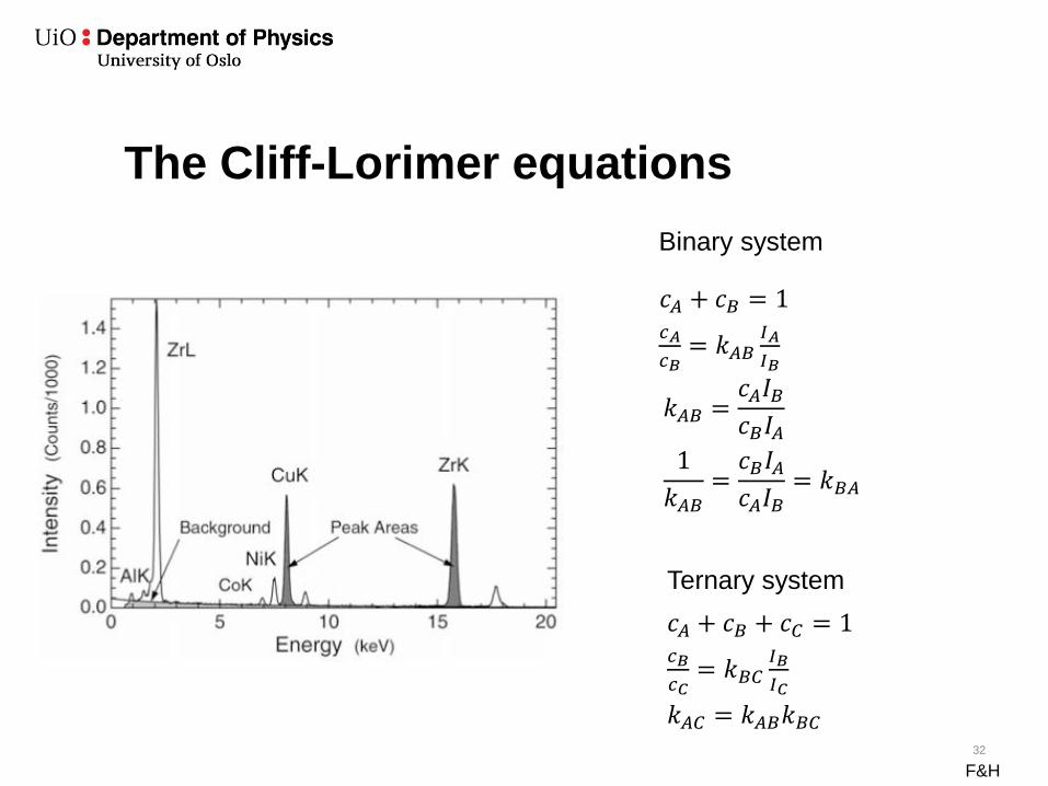
The Cliff-Lorimer equations

F&H

32

𝑐𝐴

𝑐𝐵= 𝑘𝐴𝐵

𝐼𝐴

𝐼𝐵

𝑘𝐴𝐵 =𝑐𝐴𝐼𝐵𝑐𝐵𝐼𝐴

1

𝑘𝐴𝐵=𝑐𝐵𝐼𝐴𝑐𝐴𝐼𝐵= 𝑘𝐵𝐴

𝑐𝐴 + 𝑐𝐵 = 1

𝑐𝐵

𝑐𝐶= 𝑘𝐵𝐶

𝐼𝐵

𝐼𝐶

𝑐𝐴 + 𝑐𝐵 + 𝑐𝐶 = 1

𝑘𝐴𝐶 = 𝑘𝐴𝐵𝑘𝐵𝐶

Binary system

Ternary system

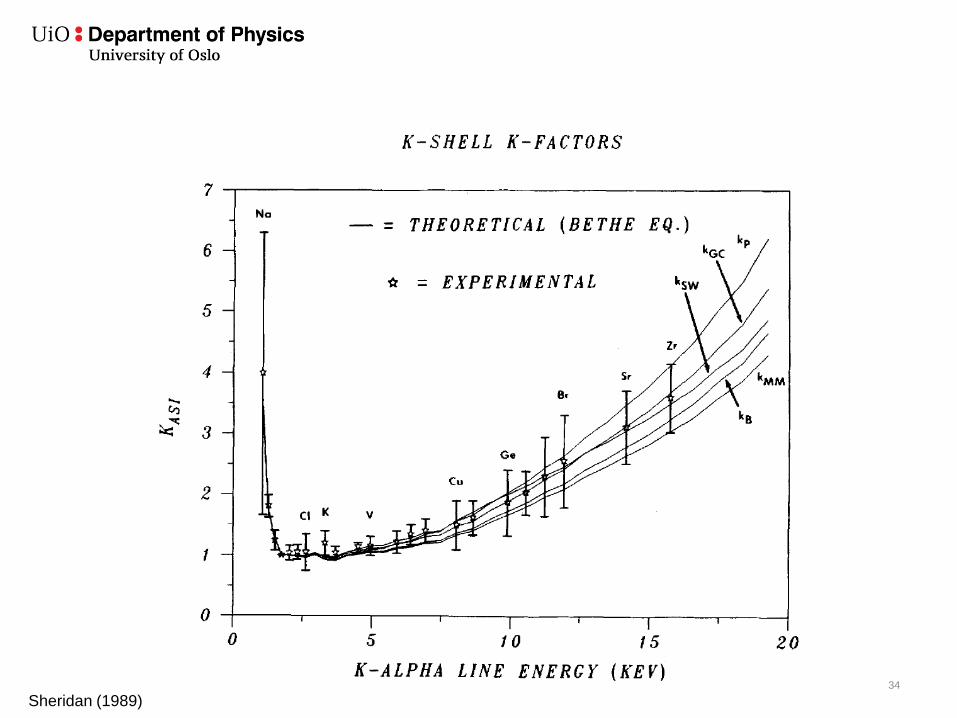
k-factors are not constants

W&C

33

34

Sheridan (1989)

k-factors are not constants

Depend on:

• Acceleration voltage

• Detector

• Analysis conditions

• Background subtraction

• Peak-integration

k-factors are a sensitivity factor for the particular system. For the best accuracy you the k-factors must be determined for the particular experimental setup.

Usually not done today, calculated k-facors used in stead. Less reliable (+/- 20%)

35

Limits to the thin film approximation

F&H

36

Limits to the thin film approximation

F&H

37

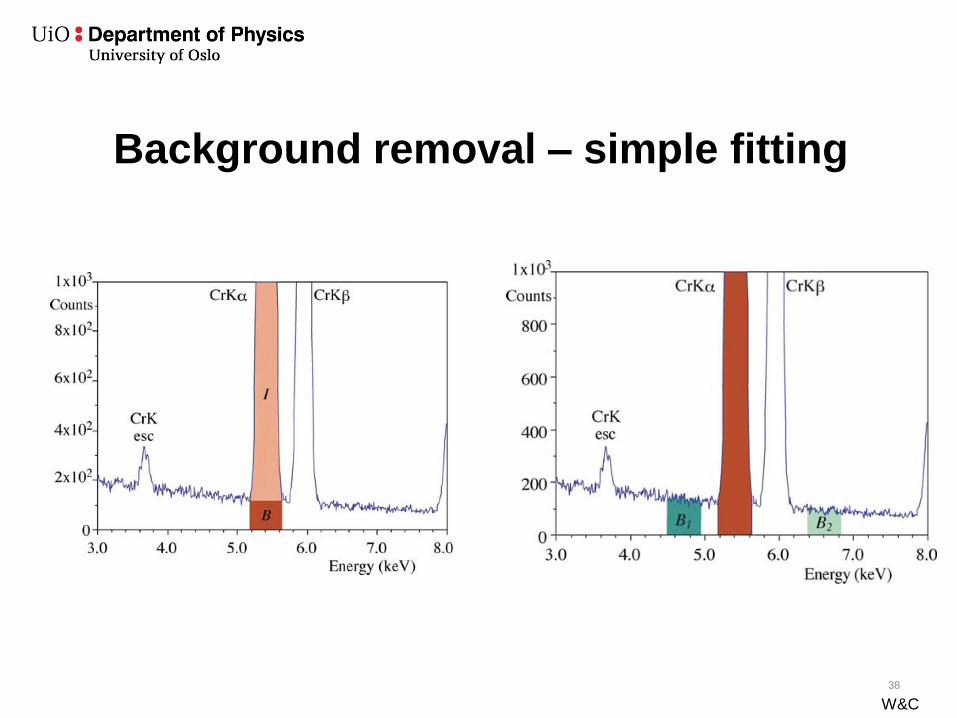
Background removal – simple fitting

W&C

38

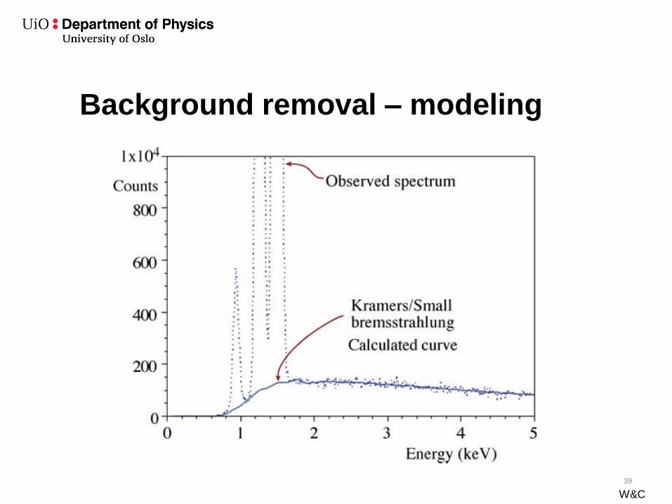
Background removal – modeling

W&C

39

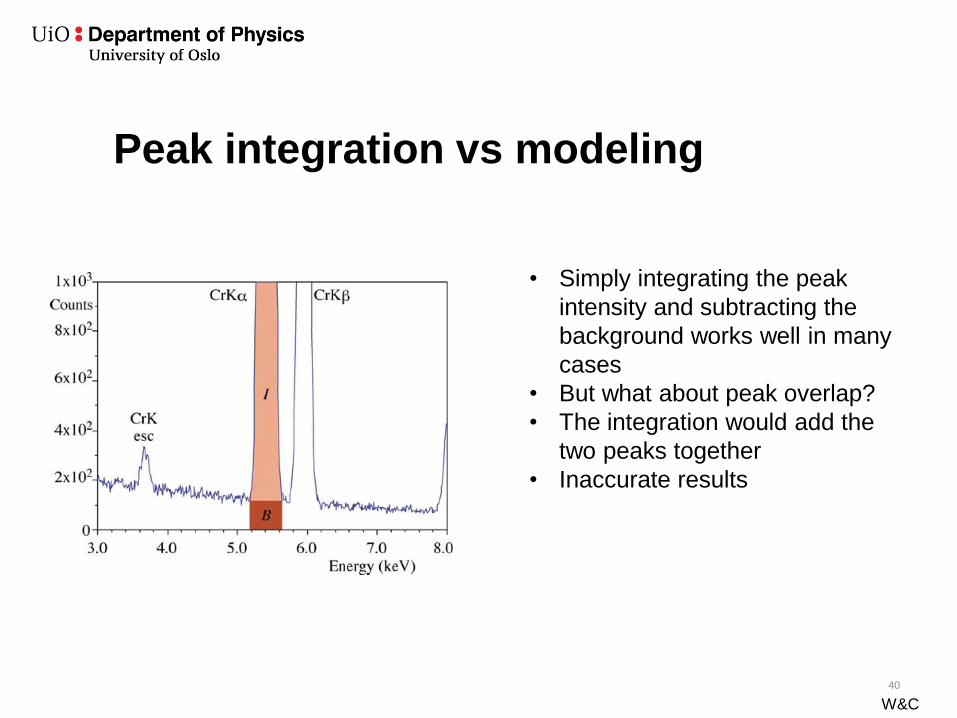
Peak integration vs modeling

• Simply integrating the peak

intensity and subtracting the

background works well in many

cases

• But what about peak overlap?

• The integration would add the

two peaks together

• Inaccurate results

W&C

40

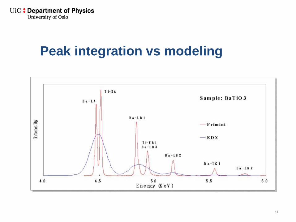
Peak integration vs modeling

41

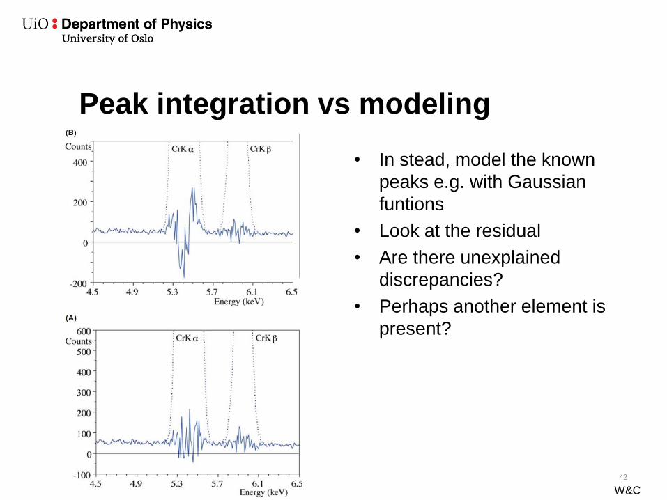
Peak integration vs modeling

• In stead, model the known

peaks e.g. with Gaussian

funtions

• Look at the residual

• Are there unexplained

discrepancies?

• Perhaps another element is

present?

W&C

42

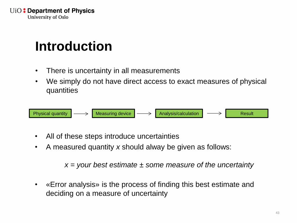
Introduction

• There is uncertainty in all measurements

• We simply do not have direct access to exact measures of physical

quantities

43

Physical quantity Measuring device Analysis/calculation Result

• All of these steps introduce uncertainties

• A measured quantity x should alway be given as follows:

x = your best estimate ± some measure of the uncertainty

• «Error analysis» is the process of finding this best estimate and

deciding on a measure of uncertainty

Measuring many times

44

200 210 220 230 240 250 260 270 280 290 3000

0.2

0.4

0.6

0.8

1

1.2

1.4

1.6

1.8

2

Measured value

Num

ber

of

measure

ments

n = 5

mean = 247.3

spread = 7.6

200 210 220 230 240 250 260 270 280 290 3000

5

10

15

20

25

30

Measured value

Num

ber

of

measure

ments

n = 150

mean = 249.1

spread = 9.8

True value= 250

𝜇 = 𝑥 =1

𝑛 𝑥𝑖

𝑛

𝑖=1

𝜎 =

1

𝑛 − 1 𝑥𝑖 − 𝑥

2

𝑛

𝑖=1

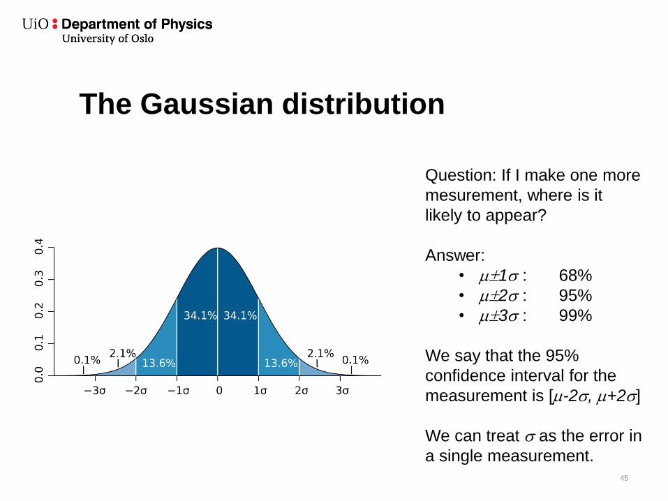
The Gaussian distribution

45

Question: If I make one more

mesurement, where is it

likely to appear?

Answer:

• 1 : 68%

• 2 : 95%

• 3 : 99%

We say that the 95%

confidence interval for the

measurement is [-2, +2]

We can treat as the error in

a single measurement.

Precision vs accuracy

46

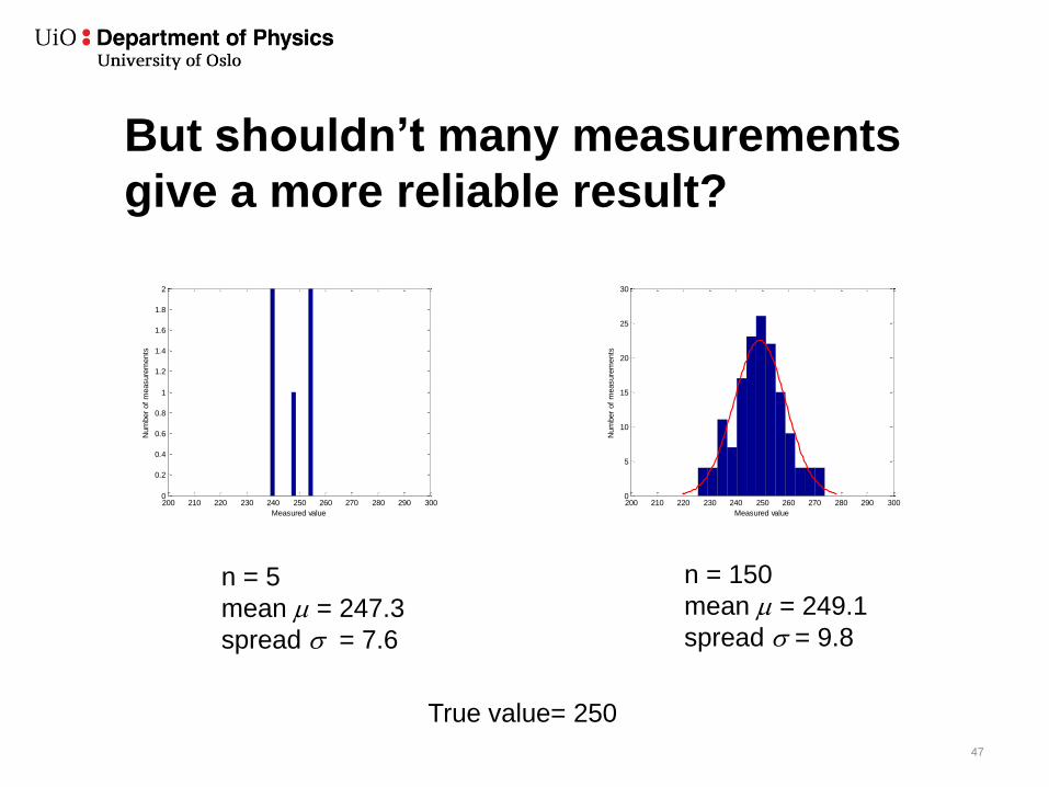
But shouldn’t many measurements

give a more reliable result?

47

200 210 220 230 240 250 260 270 280 290 3000

0.2

0.4

0.6

0.8

1

1.2

1.4

1.6

1.8

2

Measured value

Num

ber

of

measure

ments

200 210 220 230 240 250 260 270 280 290 3000

5

10

15

20

25

30

Measured value

Num

ber

of

measure

ments

True value= 250

n = 5

mean = 247.3

spread = 7.6

n = 150

mean = 249.1

spread = 9.8

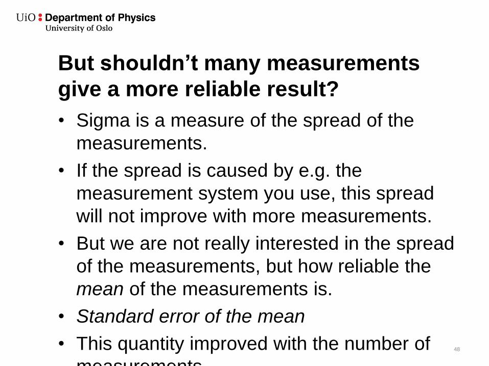
But shouldn’t many measurements

give a more reliable result?

• Sigma is a measure of the spread of the

measurements.

• If the spread is caused by e.g. the

measurement system you use, this spread

will not improve with more measurements.

• But we are not really interested in the spread

of the measurements, but how reliable the

mean of the measurements is.

• Standard error of the mean

• This quantity improved with the number of

measurements. 48

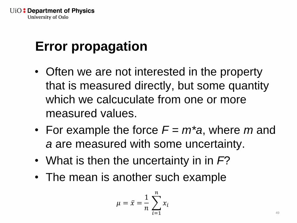
Error propagation

• Often we are not interested in the property

that is measured directly, but some quantity

which we calcuculate from one or more

measured values.

• For example the force F = m*a, where m and

a are measured with some uncertainty.

• What is then the uncertainty in in F?

• The mean is another such example

• What is the uncertainty in the mean?

49

𝜇 = 𝑥 =1

𝑛 𝑥𝑖

𝑛

𝑖=1

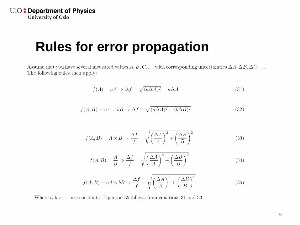
Rules for error propagation

50

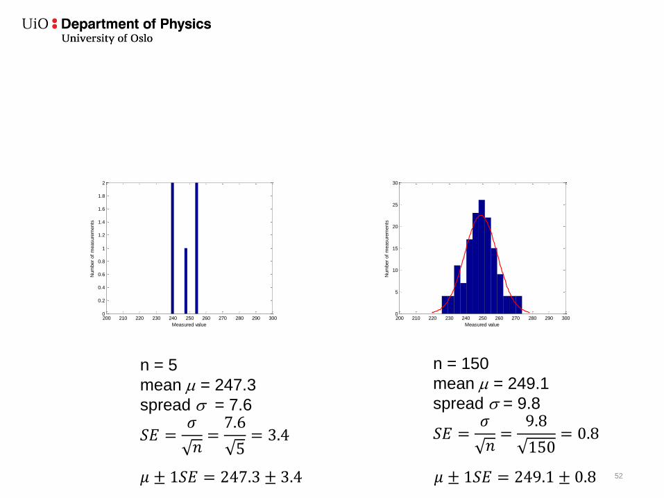
Propagating the errors in the mean

51

𝜇 = 𝑥 =1

𝑛 𝑥𝑖

𝑛

𝑖=1

=𝑥1𝑛+𝑥2𝑛+⋯+

𝑥𝑛𝑛

Assume same uncertainty in all measured xi

This is called the Standard Error in the Mean (SE)

52

200 210 220 230 240 250 260 270 280 290 3000

0.2

0.4

0.6

0.8

1

1.2

1.4

1.6

1.8

2

Measured value

Num

ber

of

measure

ments

200 210 220 230 240 250 260 270 280 290 3000

5

10

15

20

25

30

Measured value

Num

ber

of

measure

ments

𝜇 ± 1𝑆𝐸 = 247.3 ± 3.4

n = 5

mean = 247.3

spread = 7.6

𝑆𝐸 =𝜎

𝑛=7.6

5= 3.4

n = 150

mean = 249.1

spread = 9.8

𝑆𝐸 =𝜎

𝑛=9.8

150= 0.8

𝜇 ± 1𝑆𝐸 = 249.1 ± 0.8

Introduction to counting statistics

• Generation/emission of X-ray photons from an irradiated

sample is a random process with a probability p per unit time.

• For an large (infinite) counting time t, we would expect to see

N=<N>=t*p

• But what does that mean for set of a real measurements (small

t)?

• We would find N1, N2, N3, N4,..

• These values will not be equal, but will be clustered around an

average 𝑁

• For a large number of measurements, 𝑁 → 𝑁

• Counting experiments of this sort follow the Poisson distribution

• Here, the uncertainty (standard deviation) of a measurement

counting N events is estmated as 𝜎 = √(𝑁) 53

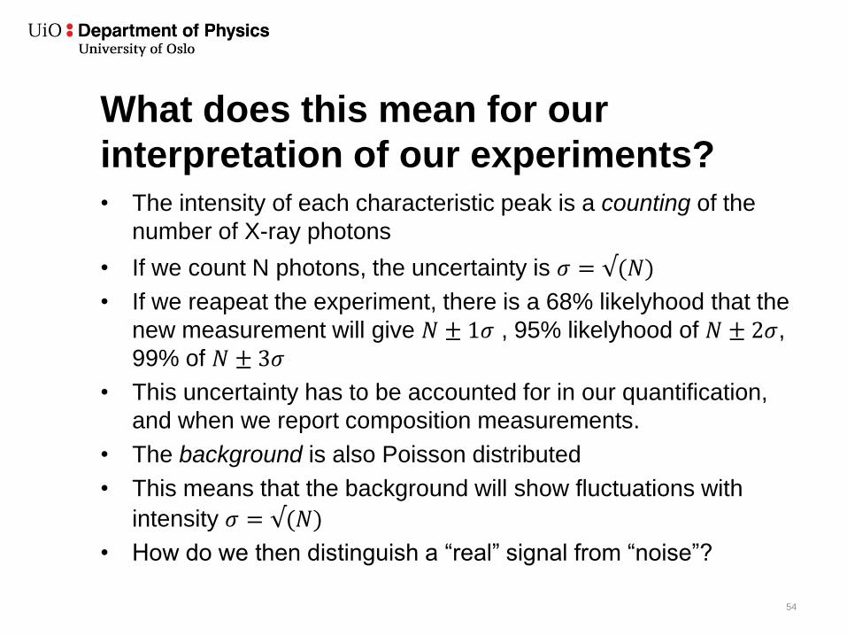
What does this mean for our

interpretation of our experiments? • The intensity of each characteristic peak is a counting of the

number of X-ray photons

• If we count N photons, the uncertainty is 𝜎 = √(𝑁)

• If we reapeat the experiment, there is a 68% likelyhood that the

new measurement will give 𝑁 ± 1𝜎 , 95% likelyhood of 𝑁 ± 2𝜎, 99% of 𝑁 ± 3𝜎

• This uncertainty has to be accounted for in our quantification,

and when we report composition measurements.

• The background is also Poisson distributed

• This means that the background will show fluctuations with

intensity 𝜎 = √(𝑁)

• How do we then distinguish a “real” signal from “noise”?

54

Significant or not?

W&C

55

Let’s quantify the ratio of Cu to Zn

• Cliff-Lorimer equations

56

𝑐𝐴

𝑐𝐵= 𝑘𝐴𝐵

𝐼𝐴

𝐼𝐵

W&C

57

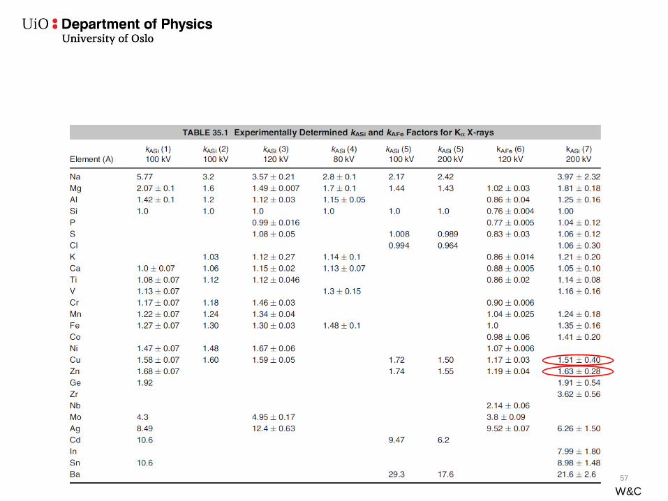
Let’s quantify the ratio of Cu to Zn

• Cliff-Lorimer equations

• 𝑘𝐶𝑢,𝑆𝑖 = 1.51 ± 0.40 2𝜎

• 𝑘𝑍𝑛,𝑆𝑖 = 1.63 ± 0.28 (2𝜎)

• 𝑘𝐶𝑢,𝑍𝑛 =?

• 𝑘𝐶𝑢,𝑍𝑛 = 𝑘𝐶𝑢,𝑆𝑖 𝑘𝑆𝑖,𝑍𝑛 = 𝑘𝐶𝑢,𝑆𝑖1

𝑘𝑍𝑛,𝑆𝑖 = 0.93

• What is 𝜎?

• 𝜎 = 0.93 0.20

1.51

2+0.14

1.63

2= 0. 15

• 𝑘𝐶𝑢,𝑍𝑛 = 0.93 ± 0.15 (1𝜎)

58

𝑐𝐴

𝑐𝐵= 𝑘𝐴𝐵

𝐼𝐴

𝐼𝐵

1

𝑘𝐴𝐵= 𝑘𝐵𝐴

𝑘𝐴𝐶 = 𝑘𝐴𝐵𝑘𝐵𝐶

59

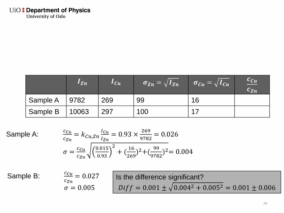
𝑰𝒁𝒏 𝑰𝑪𝒖 𝝈𝒁𝒏 = 𝑰𝒁𝒏 𝝈𝑪𝒖 = 𝑰𝑪𝒖 𝒄𝑪𝒖𝒄𝒁𝒏

Sample A 9782 269 99 16

Sample B 10063 297 100 17

Sample A: 𝑐𝐶𝑢

𝑐𝑍𝑛= 𝑘𝐶𝑢,𝑍𝑛

𝐼𝐶𝑢

𝐼𝑍𝑛= 0.93 ×

269

9782= 0.026

𝜎 =𝑐𝐶𝑢

𝑐𝑍𝑛

0.015

0.93

2+ (16

269)2+(

99

9782)2= 0.004

Sample B: 𝑐𝐶𝑢

𝑐𝑍𝑛= 0.027

𝜎 = 0.005

Is the difference significant?

𝐷𝑖𝑓𝑓 = 0.001 ± 0.0042 + 0.0052 = 0.001 ± 0.006

60

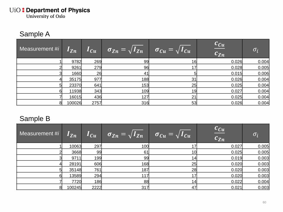
Measurement #i 𝑰𝒁𝒏 𝑰𝑪𝒖 𝝈𝒁𝒏 = 𝑰𝒁𝒏 𝝈𝑪𝒖 = 𝑰𝑪𝒖 𝒄𝑪𝒖𝒄𝒁𝒏

𝜎𝑖

1 9782 269 99 16 0.026 0.004

2 9261 279 96 17 0.028 0.005

3 1660 26 41 5 0.015 0.006

4 35175 977 188 31 0.026 0.004

5 23370 641 153 25 0.025 0.004

6 11938 343 109 19 0.027 0.004

7 16015 436 127 21 0.025 0.004

8 100026 2757 316 53 0.026 0.004

Measurement #i 𝑰𝒁𝒏 𝑰𝑪𝒖 𝝈𝒁𝒏 = 𝑰𝒁𝒏 𝝈𝑪𝒖 = 𝑰𝑪𝒖 𝒄𝑪𝒖𝒄𝒁𝒏

𝜎𝑖

1 10063 297 100 17 0.027 0.005

2 3668 99 61 10 0.025 0.005

3 9711 199 99 14 0.019 0.003

4 28191 606 168 25 0.020 0.003

5 35148 761 187 28 0.020 0.003

6 13589 294 117 17 0.020 0.003

7 7720 186 88 14 0.022 0.004

8 100245 2222 317 47 0.021 0.003

Sample A

Sample B

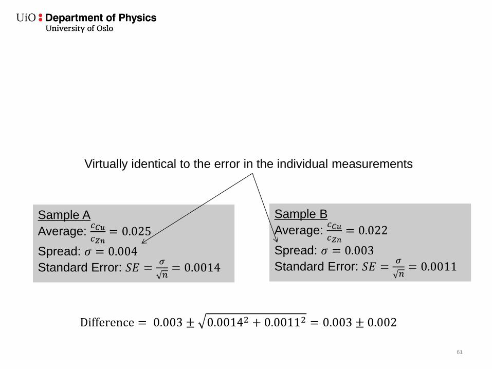
61

Sample A

Average: 𝑐𝐶𝑢

𝑐𝑍𝑛= 0.025

Spread: 𝜎 = 0.004

Standard Error: 𝑆𝐸 =𝜎

𝑛= 0.0014

Sample B

Average: 𝑐𝐶𝑢

𝑐𝑍𝑛= 0.022

Spread: 𝜎 = 0.003

Standard Error: 𝑆𝐸 =𝜎

𝑛= 0.0011

Difference = 0.003 ± 0.00142 + 0.00112 = 0.003 ± 0.002

Virtually identical to the error in the individual measurements