Embed Size (px)
Citation preview

Alma Mater Studiorum · Universita di Bologna
FACOLTA DI SCIENZE MATEMATICHE, FISICHE E NATURALI
Corso di Laurea Magistrale in Matematica
Curriculum generale-applicativo
FX MODELLING UNDER COLLATERALIZATION
Tesi di Laurea Magistrale in equazioni differenziali stocastiche
Relatore:
Chiar.mo Prof.
Andrea Pascucci
Presentata da:
Chiara Summonte
Sessione II
Anno Accademico 2015-2016


Alla mia famiglia


Contents
Introduction vii
Introduzione 1
1 Interest rate derivatives 3
1.1 Classical vs modern pricing framework . . . . . . . . . . . . . . . . . . . . . . . . . . . . . 3
1.2 Forward rates . . . . . . . . . . . . . . . . . . . . . . . . . . . . . . . . . . . . . . . . . . . 6
1.3 Forward Rate Agreements . . . . . . . . . . . . . . . . . . . . . . . . . . . . . . . . . . . . 8
1.4 Deposits . . . . . . . . . . . . . . . . . . . . . . . . . . . . . . . . . . . . . . . . . . . . . . 11
1.5 Futures . . . . . . . . . . . . . . . . . . . . . . . . . . . . . . . . . . . . . . . . . . . . . . 12
1.6 Swap . . . . . . . . . . . . . . . . . . . . . . . . . . . . . . . . . . . . . . . . . . . . . . . . 14
1.7 One-factor short rate models . . . . . . . . . . . . . . . . . . . . . . . . . . . . . . . . . . 16
1.7.1 The Vasicek model . . . . . . . . . . . . . . . . . . . . . . . . . . . . . . . . . . . . 19
1.7.2 The Hull-White model . . . . . . . . . . . . . . . . . . . . . . . . . . . . . . . . . . 21
1.7.3 An example of calibration . . . . . . . . . . . . . . . . . . . . . . . . . . . . . . . . 25
2 Funding, collateral, FVA 29
2.1 Black-Scoles-Merton from a modern perspective . . . . . . . . . . . . . . . . . . . . . . . . 29
2.2 Multiple funding sources . . . . . . . . . . . . . . . . . . . . . . . . . . . . . . . . . . . . . 33
2.3 Collateral: discrete margination . . . . . . . . . . . . . . . . . . . . . . . . . . . . . . . . . 34
2.4 Perfect collateral . . . . . . . . . . . . . . . . . . . . . . . . . . . . . . . . . . . . . . . . . 37
2.5 Perfect collateral for derivative and hedge . . . . . . . . . . . . . . . . . . . . . . . . . . . 41
2.6 Perfect collateral, dividends, repo . . . . . . . . . . . . . . . . . . . . . . . . . . . . . . . . 42
2.7 Partial collateral . . . . . . . . . . . . . . . . . . . . . . . . . . . . . . . . . . . . . . . . . 44
2.8 Perfect collateral, stochastic rates . . . . . . . . . . . . . . . . . . . . . . . . . . . . . . . . 47
2.9 General case . . . . . . . . . . . . . . . . . . . . . . . . . . . . . . . . . . . . . . . . . . . . 50
2.10 Multiple currency . . . . . . . . . . . . . . . . . . . . . . . . . . . . . . . . . . . . . . . . . 51
3 FX modelling in collateralized markets 55
3.1 Funding strategies in domestic and foreign currencies . . . . . . . . . . . . . . . . . . . . . 57
3.1.1 Collateralized foreign measure . . . . . . . . . . . . . . . . . . . . . . . . . . . . . . 58
3.2 Derivation of pricing formulae . . . . . . . . . . . . . . . . . . . . . . . . . . . . . . . . . . 59
3.2.1 Pricing domestic contracts collateralized in foreign currency . . . . . . . . . . . . . 59
3.2.2 Pricing foreign contracts collateralized in domestic or foreign currency . . . . . . . 60
3.3 Pricing FX market instruments . . . . . . . . . . . . . . . . . . . . . . . . . . . . . . . . . 61
3.3.1 Pricing FX swaps in the market practice . . . . . . . . . . . . . . . . . . . . . . . . 61
iii
3.3.2 Cross-Currency swaps . . . . . . . . . . . . . . . . . . . . . . . . . . . . . . . . . . 63
3.4 Effective discounting curve approach . . . . . . . . . . . . . . . . . . . . . . . . . . . . . . 68
3.4.1 Bootstrapping curves in the FX market . . . . . . . . . . . . . . . . . . . . . . . . 68
A Theoretical framework 71
A.1 Ito calculus: some hints. . . . . . . . . . . . . . . . . . . . . . . . . . . . . . . . . . . . . . 71
A.2 Bank account and risk neutral measure . . . . . . . . . . . . . . . . . . . . . . . . . . . . 73
A.3 Feynman-Kac theorem . . . . . . . . . . . . . . . . . . . . . . . . . . . . . . . . . . . . . . 74
A.4 Zero Coupon Bond . . . . . . . . . . . . . . . . . . . . . . . . . . . . . . . . . . . . . . . . 76
A.5 Change of measure . . . . . . . . . . . . . . . . . . . . . . . . . . . . . . . . . . . . . . . . 77
A.6 Replication . . . . . . . . . . . . . . . . . . . . . . . . . . . . . . . . . . . . . . . . . . . . 81
Bibliography 85
List of Figures
1.1 Collateral scheme . . . . . . . . . . . . . . . . . . . . . . . . . . . . . . . . . . . . . . . . . 3
1.2 Euribor6M Depo vs Eur OIS 6M (spot) rates. Quotations Jan. 2007−Jan. 2015 (source:
Bloomberg) . . . . . . . . . . . . . . . . . . . . . . . . . . . . . . . . . . . . . . . . . . . . 5
1.3 Forward Rate Agreement: market quotes . . . . . . . . . . . . . . . . . . . . . . . . . . . 10
1.4 Futures: market quotes . . . . . . . . . . . . . . . . . . . . . . . . . . . . . . . . . . . . . 13
1.5 Swap: market quotes . . . . . . . . . . . . . . . . . . . . . . . . . . . . . . . . . . . . . . . 16
3.1 A cash flow description of a constant-notional CCS . . . . . . . . . . . . . . . . . . . . . . 63
3.2 A cash flow description of a marked-to-market CCS . . . . . . . . . . . . . . . . . . . . . 63


Introduction
The financial crisis begun in the second half of 2007 has triggered, among many consequences, a
deep evolution phase of the classical framework adopted for trading derivatives. In particular, credit and
liquidity issues were found to have macroscopical impacts on the prices of financial instruments, both
plain vanillas and exotics.
Today, terminated or not the crisis, the market has learnt the lesson and persistently shows such
effects. These are clearly visible in the market quotes of plain vanilla interest rate derivatives, such as
Deposits, Forward Rate Agreements (FRA), Swaps (IRS) and options (Caps, Floors and Swaptions).
Since August 2007 the primary interest rates of the interbank market, e.g. Libor , Euribor, Eonia, and
Federal Funds rate, display large basis spreads that have raised up to 200 basis points. Recently, the
market has also included the effect of collateral agreements widely diffused among derivatives counter-
parties in the interbank market.
In this context, our aim is to describe how to coherently price derivatives with flows and/or collat-
eral posting in different currencies in presence of market dislocations and relying on funding strategies
based on FX swaps. We extend the usual arbitrage-free pricing framework to accommodate collateral ac-
counts by means of a more general definition of dividend and gain processes and we give clear definitions
of the relevant pricing measures. We finally apply these results to derive pricing formulae for derivative
contracts under different collateralization agreements.
The structure of this thesis is the following.
In Chapter 1 we start by reviewing the market practice for interest rate yield curves construction and
pricing interest rate derivatives, both in the traditional (old style) single-curve version, and in the modern
multiple-curve version triggered by the credit crunch crisis. Then we quickly describe two one-factor short
rate models, such as the Vasicek and the Hull-White models, with an example of calibration to market
data for the Vasicek model.
In Chapter 2 we derive the classical Black-Scholes-Merton pricing formulas using replication argu-
ments, PDE and Feynman-Kac. Afterwards we generalize this formula by considering more general cases
such as perfect collateral for derivative and for both derivative and hedge, derivatives on a dividend
paying asset subject to repo funding, multiple currencies, etc.
In Chapter 3, that constitutes the central contribution of this work, we start from some formulas
obtained in chapter 2 and we derive generic pricing formulae for different combinations of cash flow and
collateral currencies. Then we apply the results to the pricing of FX swaps and CCS, and we discuss curve
bootstrapping. Finally we investigate some approximations usually done in the practice when evaluating
CCS.

Introduzione
La crisi finanziaria iniziata nella seconda meta del 2007 ha innescato, tra le molte conseguenze, una
fase di profonda evoluzione del quadro classico adottato per il trading di derivati. In particolare, si e
riscontrato che i problemi di credito e liquidita hanno effetti macroscopici sui prezzi degli strumenti fi-
nanziari, sia plain vanilla sia esotici.
Oggi, terminata o no la crisi, il mercato ha imparato la lezione e mostra in modo persistente tali effetti.
Questi effetti sono chiaramente visibili nelle quotazioni di mercato dei derivati plain vanilla su tassi di
interesse, come ad esempio Depositi, Forward Rate Agreement (FRA), swap (IRS) e opzioni (cap, floor
e swaption). Dal mese di agosto 2007, i tassi di interesse primari del mercato interbancario, per esempio
Libor, Euribor, Eonia, e il tasso dei fondi federali, mostrano un ampio basis spread arrivato fino a 200
punti base. Recentemente, il mercato ha anche incluso l’effetto dei collateral agreements ampiamente
utilizzati nel mercato interbancario.
In questo contesto, il nostro scopo e quello di descrivere come prezzare coerentemente derivati con
flussi di moneta e/o collaterale postato in diverse valute, in presenza di dislocazioni di mercato e con-
tando su strategie di finanziamento basate su FX swap. Estendiamo il framework usuale di arbitrage-free
pricing per accogliere collateral accounts attraverso una piu generale definizione dei processi di dividendi
e di guadagno e diamo chiare definizioni delle misure di pricing piu rilevanti. Applichiamo infine questi
risultati per ricavare formule di pricing per contratti di derivati sotto diversi accordi di collateralizzazione.
La struttura di questa tesi e la seguente.
Nel capitolo 1 rivediamo la prassi di mercato per la costruzione delle curve dei rendimenti dei tassi di
interesse e la determinazione dei prezzi dei derivati su tassi di interesse, sia nella versione tradizionale
“single-curve” sia nella versione moderna “multiple curve” innescata dalla crisi del credito. In seguito
descriviamo rapidamente due modelli per i tassi short, come il modello di Vasicek e quello di Hull-White,
con un esempio di calibrazione ai dati di mercato per il modello di Vasicek.
Nel capitolo 2 deriviamo la formule classica di pricing di Black-Scholes-Merton utilizzando argomenti di
replicazione, PDE e Feynman-Kac. Successivamente generalizziamo questa formula considerando i casi
piu generali come perfect collateral sia per i derivati sia per la copertura, derivati su asset che pagano
dividendi soggetti a finanziamenti di tipo repo, valute multiple, ecc.
Nel capitolo 3, che costituisce il contributo centrale di questo lavoro, partiamo da alcune formule ottenuto
nel capitolo 2 e deriviamo formule generiche di pricing per combinazioni diverse di cash flow e valute per
il collaterale. Applichiamo poi i risultati al pricing dei FX swap e CCS, e discutiamo di bootstrapping.
Infine analizziamo alcune approssimazioni applicate usualmente nella valutazione dei CCS.

Chapter 1
Interest rate derivatives
1.1 Classical vs modern pricing framework
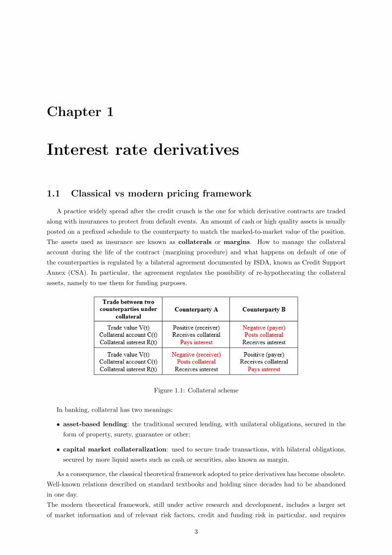
A practice widely spread after the credit crunch is the one for which derivative contracts are traded
along with insurances to protect from default events. An amount of cash or high quality assets is usually
posted on a prefixed schedule to the counterparty to match the marked-to-market value of the position.
The assets used as insurance are known as collaterals or margins. How to manage the collateral
account during the life of the contract (margining procedure) and what happens on default of one of
the counterparties is regulated by a bilateral agreement documented by ISDA, known as Credit Support
Annex (CSA). In particular, the agreement regulates the possibility of re-hypothecating the collateral
assets, namely to use them for funding purposes.
Figure 1.1: Collateral scheme
In banking, collateral has two meanings:
• asset-based lending: the traditional secured lending, with unilateral obligations, secured in the
form of property, surety, guarantee or other;
• capital market collateralization: used to secure trade transactions, with bilateral obligations,
secured by more liquid assets such as cash or securities, also known as margin.
As a consequence, the classical theoretical framework adopted to price derivatives has become obsolete.
Well-known relations described on standard textbooks and holding since decades had to be abandoned
in one day.
The modern theoretical framework, still under active research and development, includes a larger set
of market information and of relevant risk factors, credit and funding risk in particular, and requires
3

1.1 Classical vs modern pricing framework 1. Interest rate derivatives
to review “from scratch” the no-arbitrage models used on the market for derivatives’ pricing and risk
analysis.
In order to understand and to price interest rate linked instruments we must know their characteris-
tics.
• The underlying: the interest rates, such as ECB rates, Libor, Euribor, Eonia, etc.
• The money market where such interest rates are traded and the basic lending/borrowing contracts,
such as Deposits.
• The contract mechanics: the schedule with all the contract relevant dates, the payoff, and any other
condition affecting the price.
• The counterparties: leading to credit/default issues, and to the corresponding credit/debt market
(CDS and Bonds).
• The collateral: leading to liquidity/funding issues and to Central Counterparties.
• The OTC market where the basic plain vanilla derivatives, are traded used for yield curve and
volatility construction, for calibration and for hedging purposes.
• The pricing model, to calculate prices and risk measures (sensitivities, VaR, etc.)
Hence, the results of the financial crisis are several changes in the market, which can be summarized
in these stylized facts:
1. Banks are not credit risk free and are not too big to fail, credit and liquidity risk in market
benchmark interest rates (Ibor), tenor dependency.
2. Explosion of spot/forward market Ibor/OIS and Ibor/Ibor tenor basis.
3. Explosion of single and cross currency basis swap rates.
4. Break of the classic-no-arbitrage relationships between market FRA rates and forward rates implicit
in market Deposits.
1. Interest rate derivatives 5
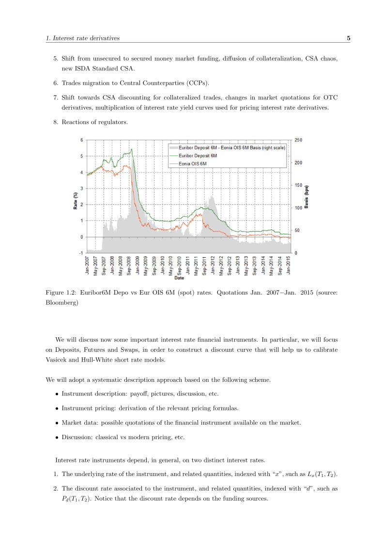
5. Shift from unsecured to secured money market funding, diffusion of collateralization, CSA chaos,
new ISDA Standard CSA.
6. Trades migration to Central Counterparties (CCPs).
7. Shift towards CSA discounting for collateralized trades, changes in market quotations for OTC
derivatives, multiplication of interest rate yield curves used for pricing interest rate derivatives.
8. Reactions of regulators.
Figure 1.2: Euribor6M Depo vs Eur OIS 6M (spot) rates. Quotations Jan. 2007−Jan. 2015 (source:
Bloomberg)
We will discuss now some important interest rate financial instruments. In particular, we will focus
on Deposits, Futures and Swaps, in order to construct a discount curve that will help us to calibrate
Vasicek and Hull-White short rate models.
We will adopt a systematic description approach based on the following scheme.
• Instrument description: payoff, pictures, discussion, etc.
• Instrument pricing: derivation of the relevant pricing formulas.
• Market data: possible quotations of the financial instrument available on the market.
• Discussion: classical vs modern pricing, etc.
Interest rate instruments depend, in general, on two distinct interest rates.
1. The underlying rate of the instrument, and related quantities, indexed with “x”, such as Lx(T1, T2).
2. The discount rate associated to the instrument, and related quantities, indexed with “d”, such as
Pd(T1, T2). Notice that the discount rate depends on the funding sources.

1.2 Forward rates 1. Interest rate derivatives
1.2 Forward rates
Forward rates F (t;Ti−1, Ti) are interest rates observed at a generic time instant t, resetting at future
time Ti−1 and spanning the future time interval [Ti−1;Ti] (called rate tenor), with t < Ti−1 < Ti. Forward
rates can be expressed in terms of Zero Coupon Bonds by recurring to a simple no-arbitrage argument.
If we define the forward Zero Coupon Bond observed at time t as
P (t;Ti−1, Ti) := EQt [P (Ti−1;Ti)]
we may write the following no arbitrage relation for deterministic N(Ti)
N(t) = P (t;Ti)N(Ti) = P (t;Ti−1)P (t;Ti−1, Ti)N(Ti)
The financial meaning of expression above is that, given a deterministic amount of money N(Ti) at time
Ti, its equivalent amount of money, or value, at time t < Ti must be unique, both if we discount directly
in one single step from Ti to t, using the discount factor P (t;Ti), and if we discount in two steps, first
from Ti to Ti−1, using the forward discount factor P (t;Ti−1, Ti) and then from Ti−1 to t, using P (t;Ti−1).
At this point we may define the simple compounded forward rate F (t;Ti−1, Ti) associated to P (t;Ti−1, Ti)
as
P (t;Ti−1, Ti) =P (t;Ti)
P (t;Ti−1):=
1
1 + F (t;Ti−1, Ti)τ(Ti−1, Ti).
By inverting we obtain the familiar no arbitrage expression
Fi(t) := F (t;Ti−1, Ti) =1
τ(Ti−1, Ti)
[1
P (t;Ti−1, Ti)− 1
]=P (t;Ti−1)− P (t;Ti)
τ(Ti−1, Ti)P (t;Ti)
We notice that, for t→ T−i−1 forward rates converge to spot Libor rates.
Theorem 1.1. Forward rates are martingales under their “natural” Ti-forward measure QTi :
Fi(t) = EQTit [Fi(u)] ∀t < u < Ti−1 < Ti
Proof. The quantity
Π(t) := P (t;Ti)Fi(t)τ(Ti−1, Ti) = P (t;Ti−1)− P (t;Ti)
is the time-t price of a tradable asset, since it is a combination of two (tradable) Zero Coupon Bonds.
Hence, under the QTi-forward measure,
Π(t)
P (t;Ti)=P (t;Ti)Fi(t)
P (t;Ti)= Fi(t) = EQTi
t
[Π(u)
P (u;Ti)
]= EQTi
t
[Fi(u)P (u;Ti)
P (u;Ti)
]= EQTi
t [Fi(u)]
In particular, setting u = Ti−1 we obtain
Fi(t) = EQTit [L(Ti−1, Ti)]

1. Interest rate derivatives 7
Notice that (risky) Libor rates Lx(Ti−1, Ti) are not martingales under the Ti-forward measure QTi ,
Fi(t) = EQTit [L(Ti−1, Ti)] 6= EQTi
t [Lx(Ti−1, Ti)] := Fx,i(t)
since the underlying Libor rate is, in general, different from the funding rate associated to the probability
measure.
We define
Fx,i(t) := EQTit [Lx(Ti−1, Ti)]
the risky forward rate.
When the funding rate and the underlying rate are the same, or in case of vanishing interest rate basis,
we obtain the classical (pre-credit crunch) single curve limit
Fx,i(t) = EQTit [Lx(Ti−1, Ti)] −→ EQTi
t [L(Ti−1, Ti)] = Fi(t)
Properties of the risky forward rate:
1. at fixing date Ti−1 it coincides with the Libor rate
Fx,i(Ti−1) = Lx(Ti−1, Ti)
2. It is a martingale under the Ti-forward discounting measure associated to the numeraire Pd(t;Ti):
Fx,i(t) = EQTit [Lx(Ti−1, Ti)] = EQTi
t [Fx,i(Ti−1)]
3. FRA contracts are quoted on the market in terms of their forward rates, thus it is “what you read
on the screen”. A forward rate term structure can be stripped from FRA quotations.
4. The risky forward rate is the basic building block of the new theoretical interest rate framework.
Instantaneous forward rate:
Instantaneous forward rates f(t;T ) are abstract forward rates observed at time t and spanning an in-
finitesimal future time interval [T ;T +dt] (with infinitesimal rate tenor). They are thus obtained through
the limit
f(t;T ) := limT ′→T+
F (t;T, T ′) = − limT ′→T+
1
P (t;T ′)
P (t;T ′)− P (t;T )
τ(T, T ′)
= − 1
P (t;T )
∂P (t;T )
∂T= −∂lnP (t;T )
∂T
Integrating the equation above we can express the Zero Coupon Bond as an integral of instantaneous
forward rates as
P (t;T ) = exp
[−∫ T
t
f(t;u)du
]Instantaneous forward rates can also be calculated as expectations of future short rates under the T -
forward measure QT . In fact, setting u = T in the martingality relation for the forward rate we obtain
f(t;T ) = EQTt [r(T )]
1.3 Forward Rate Agreements 1. Interest rate derivatives
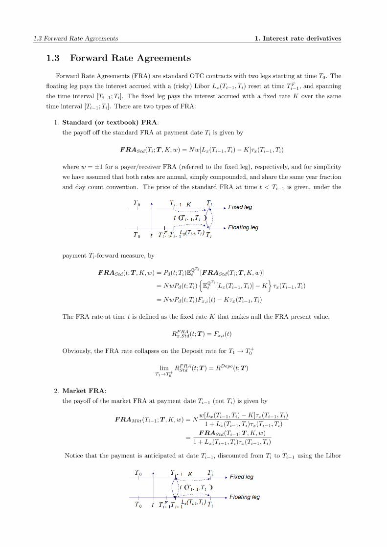
1.3 Forward Rate Agreements
Forward Rate Agreements (FRA) are standard OTC contracts with two legs starting at time T0. The
floating leg pays the interest accrued with a (risky) Libor Lx(Ti−1, Ti) reset at time TFi−1, and spanning
the time interval [Ti−1;Ti]. The fixed leg pays the interest accrued with a fixed rate K over the same
time interval [Ti−1;Ti]. There are two types of FRA:
1. Standard (or textbook) FRA:
the payoff off the standard FRA at payment date Ti is given by
FRAStd(Ti;T ,K,w) = Nw[Lx(Ti−1, Ti)−K]τx(Ti−1, Ti)
where w = ±1 for a payer/receiver FRA (referred to the fixed leg), respectively, and for simplicity
we have assumed that both rates are annual, simply compounded, and share the same year fraction
and day count convention. The price of the standard FRA at time t < Ti−1 is given, under the
payment Ti-forward measure, by
FRAStd(t;T ,K,w) = Pd(t;Ti)EQTit [FRAStd(Ti;T ,K,w)]
= NwPd(t;Ti)EQTit [Lx(Ti−1, Ti)]−K
τx(Ti−1, Ti)
= NwPd(t;Ti)Fx,i(t)−Kτx(Ti−1, Ti)
The FRA rate at time t is defined as the fixed rate K that makes null the FRA present value,
RFRAx,Std(t;T ) = Fx,i(t)
Obviously, the FRA rate collapses on the Deposit rate for T1 → T+0
limT1→T+
0
RFRAStd (t;T ) = RDepo(t;T )
2. Market FRA:
the payoff of the market FRA at payment date Ti−1 (not Ti) is given by
FRAMkt(Ti−1;T ,K,w) = Nw[Lx(Ti−1, Ti)−K]τx(Ti−1, Ti)
1 + Lx(Ti−1, Ti)τx(Ti−1, Ti)
=FRAStd(Ti−1;T ,K,w)
1 + Lx(Ti−1, Ti)τx(Ti−1, Ti)
Notice that the payment is anticipated at date Ti−1, discounted from Ti to Ti−1 using the Libor

1. Interest rate derivatives 9
rate itself.
The price of the market FRA at time t < Ti is given, under the payment Ti−1 forward measure, by
FRAMkt(t;T ,K,w) = Pd(t;Ti−1)EQTi−1
t [FRAMkt(Ti−1;T ,K,w)]
= NwPd(t;Ti−1)EQTi−1
t
[Lx(Ti−1, Ti)−K]τx(Ti−1, Ti)
1 + Lx(Ti−1, Ti)τx(Ti−1, Ti)
= NwPd(t;Ti−1)
1− [1 +Kτx(Ti−1, Ti)]EQTi−1
t
[1
1 + Lx(Ti−1, Ti)τx(Ti−1, Ti)
]Notice that, in this case, the price depends on the expectation of the forward discount factor
Px(Ti−1, Ti) :=1
1 + Lx(Ti−1, Ti)τx(Ti−1, Ti)
under the payment Ti−1 forward measure.
Switching from Ti−1 to Ti forward measure we obtain
EQTi−1
t
[1
1 + Lx(Ti−1, Ti)τx(Ti−1, Ti)
]=Pd(t;Ti−1)
Pd(t, Ti)EQTit
[1
Pd(Ti−1, Ti)
1
1 + Lx(Ti−1, Ti)τx(Ti−1, Ti)
]=
=1
1 + τd(Ti−1, Ti)Fd,i(t)EQTit
[1 + Ld(Ti−1, Ti)τd(Ti−1, Ti)
1 + Lx(Ti−1, Ti)τx(Ti−1, Ti)
]
FRAMkt(t;T ,K,w) = NwPd(t;Ti−1)
1− 1 +Kτx(Ti−1, Ti)
1 + Fd,i(t)τd(Ti−1, Ti)
EQTit
[1 + Ld(Ti−1, Ti)τd(Ti−1, Ti)
1 + Lx(Ti−1, Ti)τx(Ti−1, Ti)
]
RFRAx,Mkt(t;T ) =1
τx(Ti−1, Ti)
1 + Fd,i(t)τd(Ti−1, Ti)
EQTit
[1+Ld(Ti−1,Ti)τd(Ti−1,Ti)1+Lx(Ti−1,Ti)τx(Ti−1,Ti)
]
Thus the price of the market FRA depends on the model chosen for the joint distribution of the two
Libor rates Ld(Ti−1, Ti) and Lx(Ti−1, Ti) under the forward measure QTi .Assuming some model for the dynamics of Ld(Ti−1, Ti) and Lx(Ti−1, Ti) under the forward measure QTidwe obtain
EQTit
[1 + Ld(Ti−1, Ti)τd(Ti−1, Ti)
1 + Lx(Ti−1, Ti)τx(Ti−1, Ti)
]=
1 + Fd,i(t)τd(Ti−1, Ti)
1 + Fx,i(t)τx(Ti−1, Ti)eC
FRAx (t;Ti−1)
FRAMkt(t;T ,K,w) = NwPd(t;Ti−1)
[1− 1 +Kτx(Ti−1, Ti)
1 + Fx,i(t)τx(Ti−1, Ti)eC
FRAx (t;Ti−1)
]where Cx(t;Ti−1) is a convexity adjustment, whose detailed expression depends on the chosen model.
A possible choice is that of Mercurio (2010), in which the two FRA rates are modeled as shifted lognormal
martingales under the forward measure QTi ,
dFd,i(t)
Fd,i(t) + 1τd(Ti−1,Ti)
= σd,idWQTi
d (t)
dFx,i(t)
Fx,i(t) + 1τx(Ti−1,Ti)
= σx,idWQTix (t)
dWQTi
d (t)dWQTix (t) = ρd,x,idt
C(t;Ti−1) = [σ2x,i − σx,iσd,iρd,x,i]τ(t, Ti−1)
The size of the convexity adjustment results to be below 1 bp, even for long maturities, for typical post
credit crunch market situations1.
1see Mercurio 2010

1.3 Forward Rate Agreements 1. Interest rate derivatives
Figure 1.3: Forward Rate Agreement: market quotes
In the classical, single-curve limit, with vanishing interest rate basis, we have
FRAStd(t;T ,K,w)→ NwP (t;Ti)[Fi(t)−K]τ(Ti−1, Ti)
FRAMkt(t;T ,K,w)→ NwP (t;Ti−1)
[1− 1 + τ(Ti−1, Ti)K
1 + τ(Ti−1, Ti)Fi(t)
]=
= NwP (t;Ti)[Fi(t)−K]τ(Ti−1, Ti)
= FRAStd(t;T ,K,w)
RFRAMkt (t;T )→ RFRAStd (t;T ) = Fi(t) =1
τ(Ti−1, Ti)
[P (t;Ti−1)
P (t;Ti)− 1
]
Forward Rate Agreement pricing formulas
Classical (single-curve)
FRAStd(t;Ti−1, Ti,K,w) = NwP (t;Ti)[Fi(t)−K]τ(Ti−1, Ti)
RFRAStd (t;T ) = Fi(t) = EQTi
t [L(Ti−1, Ti)]
FRAMkt(t;Ti−1, Ti,K,w) = FRAStd(t;Ti−1, Ti,K,w)
RFRAMkt (t;T ) = RFRAStd (t;T )
Modern (multi-curve)
FRAStd(t;Ti−1, Ti,K,w) = NwPd(t;Ti)[Fx,i(t)−K]τx(Ti−1, Ti)
RFRAx,Std(t;T ) = Fx,i(t) := EQTi
t [Lx(Ti−1, Ti)]
FRAMkt(t;T ,K,w) = NwPd(t;Ti−1)[1− 1+Kτx(Ti−1,Ti)
1+Fx,i(t)τx(Ti−1,Ti)eC
FRAx (t;Ti−1)
]RFRAx,Mkt(t;T ) = 1
τx(Ti−1,Ti)
[1 + τx(Ti−1, Ti)Fx,i(t)]e
CFRAx (t;Ti−1) − 1

1. Interest rate derivatives 11
1.4 Deposits
Interest Rate Certificates of Deposits are standard OTC zero coupon contracts such that:
• at start date T0, counterparty A, called the lender, pays a nominal amount N to counterparty B,
called the borrower,
• at maturity date T the borrower pays back to the lender the nominal amount N plus the interest
accrued over the period [T0, T ] (called rate tenor) at the annual simply compounded interest rate
R(T0, T ), fixed at time TF0 < T0, where [TF0 , T0] is the settlement period, usually equal to two
working days in the EUR market.
The payoff at maturity, from the point of view of the lender (the receiver of the nominal amount plus
interests), is given by
Depo(T ;T ) = N [1 +R(T0, T )τ(T0, T )]
The price at time t, such that T0 ≤ t ≤ T , when the deposit rate R(T0, T ) is already fixed, is given
by:
• the future cash flows (the nominal amount and the interest amount), which, in this case, are
deterministic and happen at the same cash flow date T ,
• each discounted at the pricing date t ≤ T
In formulas:
Depo(T ;T ) = NP (t;T )[1 +R(T0, T )τ(T0, T )]
where P (t;T ) is a discount factor taking into account the time value of money. In case of Deposits, the
discount factor is typically consistent with the deposit rate R(t, T ) quoted on the market at time t, such
that
P (t;T ) =1
1 +R(t, T )τ(t, T ), T0 ≤ t ≤ T
This price is the same for all counterparties.

1.5 Futures 1. Interest rate derivatives
1.5 Futures
Interest rate Futures are the exchange-traded contracts on the 3 month interest rate (for example
LIBOR futures are on the 3 month LIBOR rate). They are similar to FRAs, except that their terms
(such as maturity dates) are regulated by the exchange.The Futures’ payoff at the last settlement date
Ti−1, is given by
Futures(Ti−1,T ) = N [1− Lx(Ti−1, Ti)]
This payoff is a classical example of ”mixing apples and oranges” because, clearly, on the r.h.s. 1 is
adimensional while the Libor rate Lx(Ti−1, Ti) has dimension t− 1 and they cannot be directly summed
together without an year fraction t(Ti−1, Ti). Thus we must look at it as a mere rule for computing the
amount of currency to be margined everyday.
The Futures’ price at time t < Ti−1 is given by
Futures(t,T ) = EQt [Dd(t; t)Futures(Ti−1;T )]
= N
1− EQt [Lx(Ti−1, Ti)]
:= N [1−RFutx (t;T )]
under the risk neutral measure Q associated to the funding bank account B(t). Notice that the Futures’
daily margination mechanism implies that the payoff is regulated everyday, thus generating the unitary
discount factor D(t; t) = 1 appearing in the first line above. The daily margination amount is calculated
as D = 1.000.000 · (Ptoday−Pyesterday)4 .
Hence, in order to price Futures we have to compute the Futures’ rate
RFut(t;Ti−1, Ti) := EQt [Lx(Ti−1, Ti)] = EQ
t [Fx,i(Ti−1)]
Since the forward rate Fx,i(t) is not a martingale under the risk neutral measure Q , such computation
requires the adoption of a model for the dynamics of Fx,i(t). In general, we obtain that the Futures’ rate
is given by the corresponding (risky) forward rate corrected with a convexity adjustment
RFutx (t;T ) := EQt [Lx(Ti−1, Ti)] = EQTi
t [Lx(Ti−1, Ti)] + CFutx (t, Ti−1) = Fx,i(t) + CFutx (t, Ti−1)
The expression of the convexity adjustment will depend on the particular model adopted and will contain,
in general, the model’s volatilities and correlations. For instance, under the multiple curve Libor Market
Model of Mercurio (2009), the convexity adjustment takes the form
CFutx (t, Ti−1) ∼= Fx,i(t)exp[∫ Ti−1
t
µx,i(u)du− 1]
where
∫ Ti−1
t
µx,i(u)du ∼= σx,i
i∑j=1
τd,jσd,jρx,dd,jFd,j(t)
1 + τd,jFd,j(t)(Tj−1 − t)
dFx,i(t)
Fx,i= µx,i(t)dt+ σx,idW
QTix (t)
dFd,i(t)
Fd,i= µd,i(t)dt+ σd,idW
QTi
d (t)
Fd,j(t) : = EQTjt [Ld(Tj−1, Tj)] =
1
τd,j
[Pd(t;Tj−1)
Pd(t;Tj)− 1]
σx,i, σd,j , ρx,di,j = instantaneous (deterministic) volatilities
and correlation of Fx,i(t), Fd,j(t)respectively.

1. Interest rate derivatives 13
Futures pricing formulas
Classical Futures(t,T ) = N [1−RFut(t;T )]
(single-curve) RFut(t;T ) := EQt [L(Ti−1, Ti)] = Fi(t) + CFut(t, Ti−1)
Modern Futures(t,T ) = N [1−RFutx (t;T )]
(multi-curve) RFutx (t;T ) := EQt [Lx(Ti−1, Ti)] = Fx,i(t) + CFutx (t, Ti−1)
Figure 1.4: Futures: market quotes

1.6 Swap 1. Interest rate derivatives
1.6 Swap
Interest rate swaps are OTC contracts in which two counterparties agree to exchange two streams of
cash flows, typically tied to a fixed rate K against floating rate. These payment streams are called fixed
and floating leg of the swap, respectively, and they are characterized by two schedules S, T and coupon
payoffs.
S = S0, ..., Sn,fixed leg schedule
T = T0, ..., Tm,floating leg schedule
S0 = T0, Sn = Tm
Swapletfix(Si;Si−1, Si,K) = NKτK(Si−1, Si)
Swapletfloat(Tj ;Tj−1, Ti) = NLx(Tj−1, Tj)τL(Tj−1, Tj)
where τK and τL are the year fractions with the fixed and floating rate conventions.
The fixed vs floating interest rate swap coupon payoffs are
Swapletfix(Si;Si−1, Si,K) = NKτK(Si−1, Si), i = 1, ..., n
Swapletfloat(Tj ;Tj−1, Tj) = NLx(Tj−1, Tj)τx(Tj−1, Tj), j = 1, ...,m
The coupon prices at time t < max(Si, Tj) are given by
Swapletfix(t;Si−1, Si,K) = Pd(t;Si)EQSit [Swapletfix(Si;Si−1, Si,K)]
= NPd(t;Si)KτK(Si−1, Si)
Swapletfloat(t;Tj−1, Tj) = Pd(t;Tj)EQTjt [Swapletfloat(Tj ;Tj−1, Tj)]
= NPd(t;Tj)Fx,j(t)τx(Tj−1, Tj)
The price of the fixed and floating swap legs is given, at time t < T0, by
Swapfix(t;S,K) =
n∑i=1
Swapletfix(t;Si−1, Si,K) = KAd(t,S)
Swapfloat(t;T ) =
m∑j=1
Swapletfloat(t;Tj−1, Tj)
=
m∑j=1
Pd(t;Tj)Fx,j(t)τx(Tj−1, Tj)
where the swap annuity Ad(t,S) is defined as
Ad(t,S) =
n∑i=1
Pd(t;Si)τK(Si−1, Si)
1. Interest rate derivatives 15
The index ′′d′′ reminds that the annuity is linked to the discount rate.
The total swap price is given, at time t < T0, by
Swap(t,T ,S,K, ω) = ω[Swapfloat(t;T )− Swapfix(t;S,K)]
= Nω
m∑j=1
Pd(t;Tj)Fx,j(t)τx(Tj−1, Tj)−KAd(t,S)
where ω = ±1 for a payer/receiver swap (referred to the fixed leg).
The swap rate at time t is
RSwapx (t;T ,S) =Swapfloat(t;T )
NωAd(t,S)
=
∑mj=1 Pd(t;Tj)Fx,j(t)τx(Tj−1, Tj)
Ad(t,S)
Hence the swap price can be written in terms of the swap rate as
Swap(t,T ,S,K, ω) = Nω[RSwapx (t;T ,S)−K]Ad(t,S)
In the classical, single-curve limit, with vanishing interest rate basis, we have
Swapfix(t;S,K)→NKA(t,S)
Swapfloat(t;T )→Nm∑j=1
P (t;Tj)F (t)τL(Tj−1, Tj)
∼=Nm∑j=1
[P (t, Tj−1 − P (t, Tj)] = N [P (t, T0)− P (t, Tm)]
where we have used, in the last line, the single-curve expression of the forward rate and the telescopic
property of the summation. The latter does hold exactly only if the floating leg schedule is regular (the
periods do concatenate exactly with no gaps or overlappings). In practice the error is very small (of the
order of 0.1 basis points).
The swap price and swap rate are given by
Swap(t,T ,S,K, ω) ∼= Nω[P (t, T0)− P (t, Tm)−KA(t,S)]
RSwap(t,T ,S) ∼=P (t, T0)− P (t, Tm)
A(t,S)
Swap pricing formulas
Classical Swap(t,T ,S,K, ω) = Nω[RSwap(t;T ,S)−K]Ad(t,S)
(single-curve) RSwap(t;T ,S) ∼= P (t,T0)−P (t,Tm)A(t,S)
Modern Swap(t,T ,S,K, ω) = Nω[RSwapx (t;T ,S)−K]Ad(t,S)
(multi-curve) RSwapx (t;T ,S) =∑mj=1 Pd(t;Tj)Fx,j(t)τx(Tj−1,Tj)
Ad(t,S)
1.7 One-factor short rate models 1. Interest rate derivatives
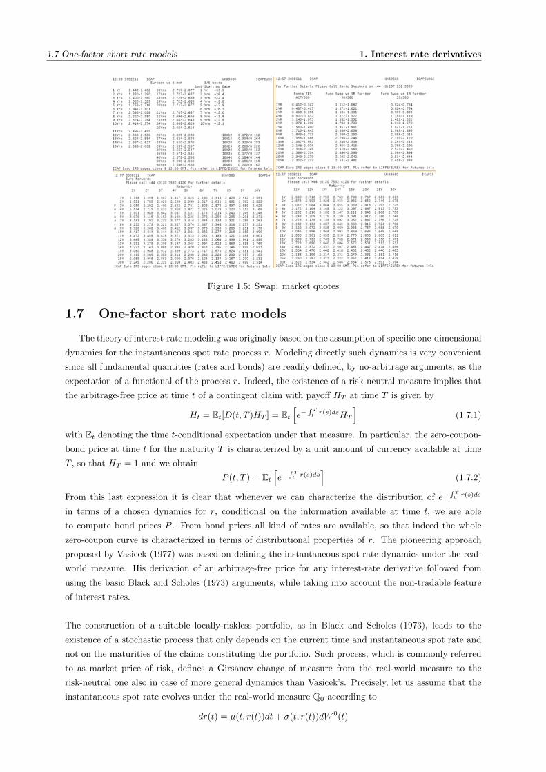
Figure 1.5: Swap: market quotes
1.7 One-factor short rate models
The theory of interest-rate modeling was originally based on the assumption of specific one-dimensional
dynamics for the instantaneous spot rate process r. Modeling directly such dynamics is very convenient
since all fundamental quantities (rates and bonds) are readily defined, by no-arbitrage arguments, as the
expectation of a functional of the process r. Indeed, the existence of a risk-neutral measure implies that
the arbitrage-free price at time t of a contingent claim with payoff HT at time T is given by
Ht = Et[D(t, T )HT ] = Et[e−
∫ Ttr(s)dsHT
](1.7.1)
with Et denoting the time t-conditional expectation under that measure. In particular, the zero-coupon-
bond price at time t for the maturity T is characterized by a unit amount of currency available at time
T , so that HT = 1 and we obtain
P (t, T ) = Et[e−
∫ Ttr(s)ds
](1.7.2)
From this last expression it is clear that whenever we can characterize the distribution of e−∫ Ttr(s)ds
in terms of a chosen dynamics for r, conditional on the information available at time t, we are able
to compute bond prices P . From bond prices all kind of rates are available, so that indeed the whole
zero-coupon curve is characterized in terms of distributional properties of r. The pioneering approach
proposed by Vasicek (1977) was based on defining the instantaneous-spot-rate dynamics under the real-
world measure. His derivation of an arbitrage-free price for any interest-rate derivative followed from
using the basic Black and Scholes (1973) arguments, while taking into account the non-tradable feature
of interest rates.
The construction of a suitable locally-riskless portfolio, as in Black and Scholes (1973), leads to the
existence of a stochastic process that only depends on the current time and instantaneous spot rate and
not on the maturities of the claims constituting the portfolio. Such process, which is commonly referred
to as market price of risk, defines a Girsanov change of measure from the real-world measure to the
risk-neutral one also in case of more general dynamics than Vasicek’s. Precisely, let us assume that the
instantaneous spot rate evolves under the real-world measure Q0 according to
dr(t) = µ(t, r(t))dt+ σ(t, r(t))dW 0(t)
1. Interest rate derivatives 17
where µ and σ are well-behaved functions and W 0 is a Q0-Brownian motion. It is possible to show2 the
existence of a stochastic process λ such that if
dP (t, T ) = µT (t, r(t))dt+ σT (t, r(t))dW 0(t) (1.7.3)
thenµT (t, r(t))− r(t)P (t, T )
σT (t, r(t))= λ(t)
for each maturity T , with λ that may depend on r but not on T . Moreover, there exists a measure Qthat is equivalent to Q0 and is defined by the Radon-Nikodym derivative
dQ
dQ0
∣∣∣∣Ft
= exp
(−1
2
∫ t
0
λ2(s)ds−∫ t
0
λ(s)dW 0(s)
)where W (t) = W 0(t) +
∫ t0λ(s)ds is a Brownian motion under Q. The equation (1.7.3) expresses the
bond-price dynamics in terms of the short rate r. It expresses how the bond price P evolves over time.
Now recall that r is the instantaneous-return rate of a risk-free investment, so that the difference µ − rrepresents a difference in returns. It tells us how much better we are doing with respect to the risk-free
case, i.e. with respect to putting our money in a riskless bank account. When we divide this quantity
by σT , we are dividing by the amount of risk we are subject to, as measured by the bond-price volatility
σT . This is why λ is referred to as “market price of risk”. An alternative term could be “excess return
with respect to a risk-free investment per unit of risk”. The crucial observation is that in order to specify
completely the model, we have to provide λ. In effect, the market price of risk λ connects the real-world
measure to the risk-neutral measure as the main ingredient in the mathematical object dQdQ0 expressing the
connection between these two “worlds”. The way of moving from one world to the other is characterized
by our choice of λ. However, if we are just concerned with the pricing of (interestrate) derivatives, we
can directly model the rate dynamics under the measure Q, so that λ will be implicit in our dynam-
ics. We put ourselves in the world Q and we do not bother about the way of moving to the world Q0.
Then we would be in troubles only if we needed to move under the objective measure, but for pricing
derivatives, the objective measure is not necessary, so that we can safely ignore it. Indeed, the value of
the model parameters under the risk-neutral measure Q is what really matters in the pricing procedure,
given also that the zero-coupon bonds are themselves derivatives under the above framework. All the
models we consider in this chapter are presented under the risk-neutral measure, even when their original
formulation was under the measure Q0. We will hint at the relationship between the two measures only
occasionally, and will explore the interaction of the dynamics under the two different measures in the
Vasicek case as an illustration.
We introduce in particular the classical short-rate model: the Vasicek model (1977), which is an
endogenous term-structure model, meaning that the current term structure of rates is an output rather
than an input of the model. The Vasicek model will be defined, under the risk-neutral measure Q, by
the dynamics
dr(t) = k[θ − r(t)]dt+ σdW (t), r(0) = r0
This dynamics has some peculiarities that make the model attractive. The equation is linear and can
be solved explicitly, the distribution of the short rate is Gaussian, and both the expressions and the
distributions of several useful quantities related to the interest-rate world are easily obtainable. Besides,
the endogenous nature of the model is now clear. Since the bond price P (t, T ) = Ete−
∫ Ttr(s)ds
can be
2See for instance Bjork (1997).
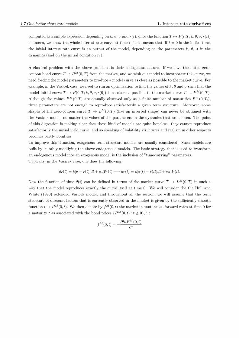
1.7 One-factor short rate models 1. Interest rate derivatives
computed as a simple expression depending on k, θ, σ and r(t), once the function T 7→ P (t, T ; k, θ, σ, r(t))
is known, we know the whole interest-rate curve at time t. This means that, if t = 0 is the initial time,
the initial interest rate curve is an output of the model, depending on the parameters k, θ, σ in the
dynamics (and on the initial condition r0).
A classical problem with the above problems is their endogenous nature. If we have the initial zero-
coupon bond curve T 7→ PM (0, T ) from the market, and we wish our model to incorporate this curve, we
need forcing the model parameters to produce a model curve as close as possible to the market curve. For
example, in the Vasicek case, we need to run an optimization to find the values of k, θ and σ such that the
model initial curve T → P (0, T ; k, θ, σ, r(0)) is as close as possible to the market curve T 7→ PM (0, T ).
Although the values PM (0, T ) are actually observed only at a finite number of maturities PM (0, Ti),
three parameters are not enough to reproduce satisfactorily a given term structure. Moreover, some
shapes of the zero-coupon curve T 7→ LM (0, T ) (like an inverted shape) can never be obtained with
the Vasicek model, no matter the values of the parameters in the dynamics that are chosen. The point
of this digression is making clear that these kind of models are quite hopeless: they cannot reproduce
satisfactorily the initial yield curve, and so speaking of volatility structures and realism in other respects
becomes partly pointless.
To improve this situation, exogenous term structure models are usually considered. Such models are
built by suitably modifying the above endogenous models. The basic strategy that is used to transform
an endogenous model into an exogenous model is the inclusion of ”time-varying” parameters.
Typically, in the Vasicek case, one does the following:
dr(t) = k[θ − r(t)]dt+ σdW (t) 7−→ dr(t) = k[θ(t)− r(t)]dt+ σdW (t).
Now the function of time θ(t) can be defined in terms of the market curve T → LM (0, T ) in such a
way that the model reproduces exactly the curve itself at time 0. We will consider the the Hull and
White (1990) extended Vasicek model, and throughout all the section, we will assume that the term
structure of discount factors that is currently observed in the market is given by the sufficiently-smooth
function t 7→ PM (0, t). We then denote by fM (0, t) the market instantaneous forward rates at time 0 for
a maturity t as associated with the bond prices PM (0, t) : t ≥ 0, i.e.
fM (0, t) = −∂lnPM (0, t)
∂t

1. Interest rate derivatives 19
1.7.1 The Vasicek model
The simplest term structure model of any practical significance is Vasicek model. Under the risk-
neutral measure its dynamics is given by:
dr(t) = k[θ − r(t)]dt+ σdW (t), r(0) = r0 (1.7.4)
where r0, k, σ are positive constants.
Integrating equation (1.7.4), we obtain, for each s ≤ t
r(t) = r(s)e−k(t−s) + θ(
1− e−k(t−s))
+ σ
∫ t
s
e−k(t−u)dW (u) (1.7.5)
so that r(t) conditional on Fs is normally distributed with mean and variance given respectively by
E[r(t)|Fs] = r(s)e−k(t−s) + θ(
1− e−k(t−s))V ar[r(t)|Fs] =
σ2
2k
[1− e−2k(t−s)
](1.7.6)
This implies that, for each time t, the rate r(t) can be negative with positive probability. The possibility
of negative rates is indeed a major drawback of the Vasicek model. However, the analytical tractability
that is implied by a Gaussian density is hardly achieved when assuming other distributions for the process
r. As a consequence of (1.7.6), the short rate r is mean reverting, since the expected rate tends, for t
going to infinity, to the value θ. The fact that θ can be regarded as a long term average rate could be
also inferred from the dynamics (1.7.4) itself. Notice, indeed, that the drift of the process r is positive
whenever the short rate is below θ and negative otherwise, so that r is pushed, at every time, to be closer
on average to the level θ. The price of a pure-discount bond can be derived by computing the expectation
(1.7.2). We obtain
P (t, T ) = A(t, T )e−B(t,T )r(t) (1.7.7)
where
A(t, T ) = exp
(θ − σ2
2k2
)[B(t, T )− T + t]− σ2
4kB(t, T )2
B(t, T ) =
1
k
[e−k(T−t)
]If we fix a maturity T , the change of numeraire3 toolkit imply that under the T -forward measure QT
dr(t) = [kθ −B(t, T )σ2 − kr(t)]dt+ σdWT (t) (1.7.8)
where the QT -Brownian motion WT is defined by
dWT (t) = dW (t) + σB(t, T )dt
so that, for s ≤ t ≤ T ,
r(t) = r(s)e−k(t−s) +MT (s, t) + σ
∫ t
s
e−k(t−u)dWT (u)
with
MT (s, t) =
(θ − σ2
k2
)(1− e−k(t−s)
)+
σ2
2k2
[e−k(T−t) − e−k(T+t−2s)
]Therefore, under QT , the transition distribution of r(t) conditional on Fs is still normal with mean and
variance given by
ET r(t)|Fs = r(s)e−k(t−s) +MT (s, t)
V arT r(t)|Fs =σ2
2k
[1− e−2k(t−s)
].
3see Appendix A.4

1.7 One-factor short rate models 1. Interest rate derivatives
The price at time t of a European option with strike X, maturity T and written on a pure discount bond
maturing at time S has been derived by Jamshidian (1989). Using the known distribution of r(t) under
QT , the calculation of the expectation (1.7.1), where HT = (P (T, S)−X)+, yields
ZBO(t, T, S,X) = w[P (t, S)Φ(wh)−XP (t, T )Φ(w(h− σp))]
where w = 1 for a call and w = −1 for a put, Φ(.) denotes the standard normal cumulative distribution
function, and
σp = σ
√1− e−2k(T−t)
2kB(T, S)
h =1
σpln
P (t, S)
P (t, T )X+σp2
We can also consider the objective measure dynamics of the Vasicek model as a proceee of the form
dr(t) = [kθ − (k + λσ)r(t)]dt+ σdW 0(t), r(0) = r0 (1.7.9)
where λ is a new parameter, contributing to the market price of risk. Compare this Q0 dynamics to the
Q-dynamics (1.7.4). Notice that for λ = 0 the two dynamics coincide, i.e. there is no difference between
the risk neutral world and the objective world. More generally, the above Q0-dynamics is expressed again
as a linear Gaussian stochastic differential equation, although it depends on the new parameter λ. This
is a tacit assumption on the form of the market price of risk process. Indeed, requiring that the dynamics
be of the same nature under the two measures, imposes a Girsanov change of measure of the following
kind to go from (1.7.4) to (1.7.9):
dQdQ0
∣∣∣∣Ft
= exp
(−1
2
∫ t
0
λ2r(s)2ds+
∫ t
0
λr(s)dW 0(s)
).
In other terms, we are assuming that the market price of risk process λ(t) has the functional form
λ(t) = λr(t)
in the short rate. Of course, in general there is no reason why this should be the case. However, under
this choice we obtain a short rate process that is tractable under both measures.

1. Interest rate derivatives 21
1.7.2 The Hull-White model
The need for an exact fit to the currently-observed yield curve, led Hull and White to the introduction
of a time-varying parameter in the Vasicek model. Notice indeed that matching the model and the market
term structures of rates at the current time is equivalent to solving a system with an infinite number of
equations, one for each possible maturity. Such a system can be solved in general only after introducing
an infinite number of parameters, or equivalently a deterministic function of time.
In this section we stick to the extension where only one parameter, corresponding to the Vasicek θ, is
chosen to be a deterministic function of time.
The model we analyze implies a normal distribution for the short-rate process at each time. Moreover,
it is quite analytically tractable in that zero-coupon bonds and options on them can be explicitly priced.
The Gaussian distribution of continuously-compounded rates then allows for the derivation of analytical
formulas and the construction of efficient numerical procedures for pricing a large variety of derivative
securities.
Hull and White (1990) assumed that the instantaneous short-rate process evolves under the risk-neutral
measure according to
dr(t) = [θ(t)− a(t)r(t)]dt+ σ(t)dW (t) (1.7.10)
where θ, a, σ are deterministic functions of time. Here we concentrate on the following extension of the
Vasicek model being analyzed by Hull and White (1994)
dr(t) = [θ(t)− ar(t)]dt+ σdW (t) (1.7.11)
where a and σ are now positive constants and θ is chosen so as to exactly fit the term structure of interest
rates being currently observed in the market. It can be shown that, denoting by fM (0, T ) the market
instantaneous forward rate at time 0 for the maturity T , i.e.,
fM (0, T ) = −∂lnPM (0, T )
∂T
with PM (0, T ) the market discount factor for the maturity T , we must have
θ(t) =∂fM (0, t)
∂T+ afM (0, t) +
σ2
2a(1− e−2at) (1.7.12)
where ∂fM
∂T denotes partial derivative of fM with respect to its second argument.
Equation (1.7.11) can be easily integrated so as to yield
r(t) = r(s)e−a(t−s) +
∫ t
s
e−a(t−u)θ(u)du+ σ
∫ t
s
e−a(t−u)dW (u) (1.7.13)
= r(s)e−a(t−s) + α(t)− α(s)e−a(t−s) + σ
∫ t
s
e−a(t−u)dW (u) (1.7.14)
where
α(t) = fM (0, t) +σ2
2a2(1− e−at)2 (1.7.15)
Therefore, r(t) conditional on Fs is normally distributed with mean and variance given respectively by
E[r(t)|Fs] = r(s)e−a(t−s) + α(t)− α(s)e−a(t−s)
V ar[r(t)|Fs] =σ2
2a
[1− e−2a(t−s)
]

1.7 One-factor short rate models 1. Interest rate derivatives
Notice that defining the process x by
dx(t) = −ax(t)dt+ σdW (t), x(0) = 0 (1.7.16)
we immediately have that, for each s < t
x(t) = x(s)e−a(t−s) + σ
∫ t
s
e−a(t−u)dW (u)
so that we can write r(t) = x(t) + α(t) for each t.
For model (1.7.11), the risk-neutral probability of negative rates at time t is explicitly given by
Qr(t) < 0 = Φ
− α(t)√α2
2a [1− e−2at]
.
However such probability is almost negligible in practice.
Bond and Option Pricing
The price at time t of a pure discount bond paying off 1 at time T is given by the expectation (1.7.2).
Such expectation is relatively easy to compute under the dynamics (1.7.11). Notice indeed that, due
to the Gaussian distribution of r(T ) conditional on Ft, t ≤ T ,∫ Ttr(u)du is itself normally distributed.
Precisely we can show that∫ T
t
r(u)du|Ft ∼ N(B(t, T )[r(t)− α(t)] + ln
PM (0, t)
PM (0, T )+
1
2[V (0, T )− V (0, t)], V (t, T )
)where
B(t, T ) =1
a
[1− e−a(T−t)
]V (t, T ) =
σ2
a2
[T − t+
2
ae−a(T−t) − 1
2ae−2a(T−t) − 3
2a
]so that we obtain
P (t, T ) = A(t, T )e−B(t,T )r(t) (1.7.17)
where
A(t, T ) =PM (0, T )
PM (0, t)exp
B(t, T )fM (0, t)− σ2
4a(1− e−2a)B(t, T )2
Similarly, the price ZBC(t, T, S,X) at time t of a European call option with strike X, maturity T and
written on a pure discount bond maturing at time S is given by the expectation
ZBC(t, T, S,X) = E(e−
∫ Ttr(s)ds(P (T, S)−X)+|Ft
)or, equivalently, by
ZBC(t, T, S,X) = P (t, T )ET ((P (T, S)−X)+|Ft).
To compute the latter expectation, we need to know the distribution of the process r under the T -forward
measure QT . Since the process x corresponds to the Vasicek’s r with θ = 0, we can use formula (1.7.8)
to get
dx(t) = [−B(t, T )σ2 − ax(t)]dt+ σdWT (t)
where the QT -Brownian mption WT is defined by dWT (t) = dW (t) + σB(t, T )dt, so that, for s ≤ t ≤ T ,
x(t) = x(s)e−a(t−s) −MT (s, t) + σ
∫ t
s
e−a(t−u)dWT (u)

1. Interest rate derivatives 23
with
MT (s, t) =σ2
a2
[1− e−a(t−s)
]− σ2
2a2
[e−a(T−t) − e−a(T+t−2s)
]It’s easy to find that the distribution of the short rate r(t) conditional on Fs is, under the measure
QT , still Gaussian with mean and variance given respectively by
ET r(t)|Fs = x(s)e−a(t−s) −MT (s, t) + α(t),
V arT r(t)|Fs =σ2
2a
[1− e−2a(t−s)
]As a consequence, the European call-option price is
ZBC(t, T, S,X) = P (t, S)Φ(h)−XP (t, T )Φ(h− σp)
where
σp = σ
√1− e−2a(T−t)
2aB(T, S)
h =1
σpln
P (t, S)
P (t, T )X+σp2
Analogously, the price ZBP (t, T, S,X) at time t of a European put option with strike X, maturity T
and written on a pure discount bond maturing at time S is given by
ZBP (t, T, S,X) = XP (t, T )Φ(−h+ σp)− P (t, S)Φ(−h).
Through these formulas we can also price caps and floors since they can be viewed as portfolios of zero-
bond options. To this end, we denote by D = d1, d2, ..., dn the set of the cap/floor payment dates
and by T = t0, t1, ..., tn the set of the corresponding times, meaning that ti is the difference in years
between di and the settlement date t, and where t0 is the first reset time. Moreover, we denote by τi the
year fraction from di−1 to di, i = 1, ..., n. So the price at time t < t0 of the cap with cap rate (strike) X,
nominal value N and set of times T is given by
Cap(t, T , N,X) = N
n∑i=1
(1 +Xτi)ZBP
(t, ti−1, ti,
1
1 +Xτi
)or, more explicitly,
Cap(t, T , N,X) = N
n∑i=1
[P (t, ti−1)Φ(−hi + σip)− (1 +Xτi)P (t, ti)Φ(−hi)]
where
σip = σ
√1− e−2a(ti−1−t)
2aB(ti−1, ti),
hi =1
σiplnP (t, ti)(1 +Xτi)
P (t, ti−1)+σip2
Analogously, the price of the corresponding floor is
F lr(t, T , N,X) = N
n∑i=1
[(1 +Xτi)P (t, ti)Φ(hi)− P (t, ti−1)Φ(hi − σip)]
We are also able to explicitly price European options on coupon-bearing bonds. To this end, consider
a European option with strike X and maturity T , written on a bond paying n coupons after the option
maturity. Denote by Ti,Ti > T , and ci the payment time and value of the i-th cash flow after T . Let

1.7 One-factor short rate models 1. Interest rate derivatives
T := T1, ..., Tn and c := c1, ..., cn. Denote by r∗ the value of the spot rate at time T for which
the coupon-bearing bond price equals the strike and by Xi the time-T value of a pure-discount bond
maturing at Ti when the spot rate is r∗. Then the option price at time t < T is
CBO(t, T, T , c,X) =
n∑i=1
ciZBO(t, T, Ti, Xi) (1.7.18)
Given the analytical formula (1.7.18), also European swaptions can be analytically priced, since a Euro-
pean swaption can be viewed as an option on a coupon-bearing bond. Indeed, consider a payer swaption
with strike rate X, maturity T and nominal value N , which gives the holder the right to enter at time
t0 = T an interest rate swap with payment times T = t1, ..., tn, t1 > T , where he pays at the fixed rate
X and receives LIBOR set “in arrears”. We denote by τi the year fraction from ti−1 to ti, i = 1, ..., n
and set ci := Xτi for i = 1, ..., n− 1 and cn := 1 +Xτi. Denoting by r∗ the value of the spot rate at time
T for whichn∑i=1
ciA(T, ti)e−B(T,ti)r
∗= 1
and setting Xi := A(T, ti)exp(B(T, ti)r∗), the swaption price at time t < T is then given by
PS(t, T, T , N,X) = N
n∑i=1
ciZBP (t, T, ti, Xi)
Analogously, the price of the corresponding receiver swaption is
RS(t, T, T , N,X) = N
n∑i=1
ciZBC(t, T, ti, Xi)
1. Interest rate derivatives 25
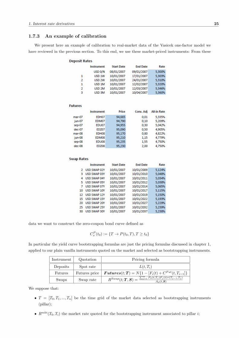
1.7.3 An example of calibration
We present here an example of calibration to real-market data of the Vasicek one-factor model we
have reviewed in the previous section. To this end, we use these market-priced instruments: From these
data we want to construct the zero-coupon bond curve defined as
CPx (t0) := T → P (t0, T ), T ≥ t0
In particular the yield curve bootstrapping formulas are just the pricing formulas discussed in chapter 1,
applied to our plain vanilla instruments quoted on the market and selected as bootstrapping instruments.
Instrument Quotation Pricing formula
Deposits Spot rate L(t, Ti)
Futures Futures price Futures(t;T ) = N1− [Fi(t) + CFut(t, Ti−1]Swaps Swap rate RSwap(t;T ,S) =
∑mj=1 Pd(t,Tj)Fj(t)τ(Tj−1,Tj)
Ad(t,S)
We suppose that:
• T = [T0, T1, ..., Tn] be the time grid of the market data selected as bootstrapping instruments
(pillar);
• Rmkt(T0, Ti) the market rate quoted for the bootstrapping instrument associated to pillar i;

1.7 One-factor short rate models 1. Interest rate derivatives
• We have already bootstrapped the yield curve until pillar i− 1 and we want to compute the curve
at pillar i.
Then, the bootstrapping algorithm proceeds as follows, for each typology of bootstrapping instruments:
• Deposits: P (t0, Ti) = 11+L(t0,Ti)τ(t0,Ti)
• Futures: P (t0, Ti) = P (t0,ti−1)
1+[1−Futures(t;T )100 −CFut(t,Ti−1)]τ(Ti−1,Ti)
• Swap: P (t0, Ti) = Pd(t0,Ti)P (t0,Ti−1)
RSwapi (t0)Ad,i(t0)−RSwapi−1 (t0)Ad,i−1(t0)+Pd(t0,Ti))
We determine the discount factors for the standard maturities in three steps:
1. Build the short end (approximately, the first 3 months) of the curve using deposit rates. This step
involve some interpolation.
2. Build the intermediate (somewhere between 3 months and 5 years) part of the curve using the
Eurodollar futures. The starting date for the first future has its discount rate set by interpolation
from the already built short end of the curve. With the addition of each consecutive future contract
to the curve the discount factor for its starting date is either (a) interpolated from the existing
curve if it starts earlier than the end date of the last contract, or (b) extrapolated from the end
date of the previous future.
3. Build the long end of the curve using swap rates as par coupon rates. Observe first that for a swap
of maturity Tmat we can calculate the discount factor P (0;Tmat) in terms of the discount factors
to the earlier coupon dates:
P (0, Tmat) =1− S(Tmat)
∑n−1j=1 αjP (0, Tj)
1 + αnS(Tmat)
We begin by interpolating the discount factors for coupon dates that fall within the previously
built segment of the curve, and continue by inductively applying the above formula. The problem
is that we do not have market data for swaps with maturities falling on all standard dates and
interpolation is again necessary to deal with the intermediate dates.
We obtain: Then, implementing the equation (1.7.7) for the price of a zero-coupon bond, our aim is to
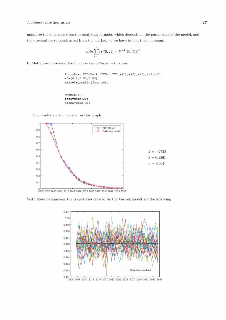
1. Interest rate derivatives 27
minimize the difference from this analytical formula, which depends on the parameters of the model, and
the discount curve constructed from the market, i.e we have to find this minimum:
min
n∑i=1
(P (0, Ti)− Pmkt(0, Ti))2
In Matlab we have used the function lsqnonlin.m in this way
Our results are summarized in this graph:
k = 0.2728
θ = 0.1861
σ = 0.001
With these parameters, the trajectories created by the Vasicek model are the following


Chapter 2
Funding, collateral, funding value
adjustment
2.1 Black-Scoles-Merton from a modern perspective
We consider a generic derivative Π depending on a single generic underlying asset A, with payoff Π(T )
at time T and price Π(t) at time t < T .
We assume a market M that trades three financial instruments:
1. the asset A, with no dividends
2. the derivative Π
3. the funding account Bf (cash) for funding unsecured at rate rf
We stress the following assumptions:
• Single asset A
• No collateral
• No counterparty risk
• No dividends
• Generic funding for asset A, no repo
• Deterministic interest rates (see the derivation)
• All the classical Black-Scholes-Merton assumptions
We will derive the classical Black-Scholes-Merton pricing formulas using replication arguments, PDE and
Feynman-Kac. In particular, we will be able to understand when and where funding enters into the
derivation and into the final result.
Dynamics under real measure P :
dA(t) = µ(t, A)dt+ σ(t, A)dWP (t)
dBf (t) = rf (t)Bf (t)dt
29

2.1 Black-Scoles-Merton from a modern perspective 2. Funding, collateral, FVA
dΠ(t) =∂Π
∂tdt+
∂Π
∂AdA(t) +
1
2
∂2Π
∂2AdA2(t)
= LµΠ(t)dt+ σ(t, A)∂Π
∂AdWP (t)
Lµ =∂Π
∂t+ µ(t, A)
∂Π
∂A+
1
2σ2(t, A)
∂2Π
∂2A
following notation and basic assumptions previously established and dropping obvious indexes.
We now construct a replication strategy Θ of the derivative Π, by setting up a replication portfolio
V such that
V (t) = Π(t), ∀t ≤ T
by combining appropriate amounts of the available assets
X(t) :=
[A(t)
Bf (t)
]
Θ(t) :=
[∆(t)
Ψf (t)
]
V (t) = Θ(t)′ ·X(t) = ∆(t)A(t) + Ψf (t)Bf (t)
where:
• X is the vector of the price processes of the assets,
• Θ is the vector of the portfolio positions, or number of units, in each asset,
• V is the (scalar) value of the replication portfolio,
• Θ(t)′ denotes vector transposition.
The replication strategy is described also by its (vector) dividend processes D(t), and gain processes G(t)
(namely profit and losses achieved by holding securities), such that
D(t) = 0
G(t) := X(t) +D(t) = X(t)
The gain processes of the assets, in SDE form, are given directly by the dynamics chosen before, as
dG(t) = dX(t) =
[dA(t)
dBf (t)
]=
[µ(t, A)dt+ σ(t, A)dWP (t)
rf (t)Bf (t)dt
]The gain process of the replication portfolio is given, in SDE form, by
dG(t) := Θ(t)′ · dG(t)
= ∆(t)dA(t) + Ψf (t)dBf (t)
= [µ(t, A)∆(t) + rf (t)Ψf (t)Bf (t)]dt+ ∆(t)σ(t, A)dWP (t)
We now impose replication condition, and we obtain
Π(t) = V (t) = ∆(t)A(t) + Ψf (t)Bf (t) ∀t ≤ T

2. Funding, collateral, FVA 31
⇒ Ψf (t)Bf (t) = Π(t)−∆(t)A(t)
consistently with the fact that the funding account Bf is used to finance the borrowing of ∆(t) units of
the underlying A(t) at the funding rate rf (t).
The gain process of the replication portfolio becomes
dG(t) := µ(t, A)∆(t)dt+ dΓ(t, A) + ∆(t)σ(t, A)dWP (t)
dΓ(t, A) = [−rf (t)∆(t)A(t) + rf (t)Π(t)]dt
the cash amount Γ(t) contained in the replication portfolio is split between:
• the derivative Π(t), growing at the funding rate rf (t),
• the amount ∆(t)A(t), borrowed at the funding rate rf (t) to finance the purchase of ∆(t) units of
the underlying asset A(t).
We now impose the self-financing condition. The replication strategy is said self-financing if its dividend
process (in/out cash flows generated by the strategy) is null,
D(t) = G(t)− V (t) = 0
We have just seen that this latter condition is already satisfied. Combining the conditions above, we have
dG(t) = dV (t) = dΠ(t)
Introducing in this latter equation the expressions of dG(t) and dΠ(t) obtained before, and rearranging
terms we obtain the SDE[∂Π
∂t+ µ(t, A)
(∂Π
∂A−∆(t)
)+
1
2σ2(t, A)
∂2Π
∂2A
]dt+ σ(t, A)
(∂Π
∂A−∆(t)
)dWP (t) = dΓ(t, A)
We finally impose the risk neutral condition ∆(t) = ∂Π∂A , such that the stochastic (risky) term with
dWP (t) disappears, and we obtain a Black-Scholes PDE equation for the derivative’s price Π(t)
LrfΠ(t) = rf (t)Π(t)
Lrf :=∂
∂t+ rf (t)A(t)
∂
∂A+
1
2σ2(t, A)
∂2
∂2A
Using the Feynman-Kac theorem we may switch from the PDE representation to the SDE representation
given by
Π(t) = EQt [Df (t;T )Π(T )]
Df (t;T ) := exp
[−∫ T
t
rf (u)du
]dA(t) = rf (t)A(t)dt+ σ(t, A)dWQ(t)
under the risk neutral funding probability measure Q associated, in this case, to the funding account
Bf (t). We conclude that we discount at the funding rate.
2.1 Black-Scoles-Merton from a modern perspective 2. Funding, collateral, FVA
Remark 2.1. Replication at work
This proof makes clear how the replication and funding mechanism works in practice. The market risk
generated by the derivatives’ position is hedged using the risky asset A. The replication strategy is
constructed with a combination of the instruments available on the market: the (single) asset A and the
funding account Bf . The former allows to include into the replication strategy the appropriate amount
of risk to hedge the risk generated by the derivative. The latter describe the amount of cash that we must
borrow or lend on the market at the funding rate rf to finance the hedging. The cash is split between
the amount ∆(t)A(t), borrowed to finance the purchase of ∆(t) units of the risky asset A(t), and the
amount Π.
Remark 2.2. Probability measure
The probability measure Q introduced via Feynman-Kac is associated to the risk neutral drift rf appearing
in the SDE dynamics of the asset A. In the classical financial world Q was traditionally associated to
a Libor Bank account, reflecting the average funding rate on the interbank money market, considered a
good proxy of a risk free rate. Nowadays, in the modern financial world, there are no risk free rates, and
Q must be interpreted simply as the risk neutral measure associated to the funding account Bf . We call
it the funding measure.
Remark 2.3. Static hedge
In particular, self-financing implies the absence of strategy dividends and
dV (t) = dG(t)
⇒ d[Θ(t)′ ·X(t)] = Θ(t)′ · dG(t) = Θ(t)′ · dX(t)
d[∆(t)A(t) + Ψf (t)Bf (t)] = ∆(t)dA(t) + Ψf (t)dBf (t)
⇒ dΘ(t) = 0
⇒ Θ(t) = constant
This is the well known feature of the classical Black-Scholes derivation:
• the position ∆(t)A(t) in the risky asset S is self-financing in its own, because its variation d[∆(t)A(t)]
is funded by the risky asset variation alone, ∆(t)dA(t).
• the position is static, ∆(t) = constant.
We stress that this is a consequence of the absence of dividends. In general this equality does not hold
d[Θ(t)′ ·X(t)] 6= Θ(t)′ · dX(t)
Remark 2.4. Zero Coupon Bond
We can define unsecured Zero Coupon Bonds, such that
Pf (T ;T ) = 1
Pf (t;T ) = EQt [Df (t;T )]
Remark 2.5. We can switch from risk neutral funding measure Q , associated to numeraire Bf (t), to
2. Funding, collateral, FVA 33
T−forward measure Q T , associated to numeraire Pf (t, T ), using the Radon-Nikodym derivative
Mf (t;T ) : =Pf (t;T )
Bf (t)
Π(t;T ) = EQt [Df (t, T )Π(T )]
= Mf (t;T )EQTt
[Df (t, T )
Mf (T ;T )Π(T )
]=Pf (t;T )
Bf (t)EQTt
[Bf (t)
Pf (T ;T )Π(T )
]= Pf (t;T )EQT
t [Π(T )]
2.2 Multiple funding sources
We assume that derivatives’ counterparties may finance their derivatives’ activity by borrowing and
lending funds on the market through a variety of market operations, such as trading Deposits, Repos
(Repurchase Agreements), Bonds, etc. at their corresponding funding rates. We also assume that deriva-
tives’ counterparties eventually reduce the counterparty risk through the adoption of bilateral collateral
agreements (CSA) or trade migration to Central Counterparties (CCPs). In particular, we will identify
three sources of funding associated with derivatives.
• Money market
Money market funding is the traditional unsecured funding source for banks and financial institu-
tions. Borrowing and lending is based on the trading of Certificates of Deposit (Depo). A Depo is
an unsecured cash zero coupon loan. In case of default of the borrower during the Depo life, the
lender suffers a loss. In banks and financial institutions, a derivative trading desk may borrow and
lend unsecured funds through a treasury desk.
• Repo market
Another common funding source is repo funding. In this case, borrowing and lending is based
on trading Repurchase Agreement contracts (Repo). A Repo is a secured cash zero coupon loan
such that, at time t, counterparty B, the borrower, sales an asset A to counterparty L, the lender,
receiving upfront the corresponding asset value A(t), under the agreement to buy it back and pay
an interest RR(t, T ), called repo rate, at maturity T > t. Thus, the borrower pays, at maturity T
the amount
ΠR(T,A) = A(t)[1 +RR(t, T )τ(t, T )]
The repo is secured by the asset A itself, used as collateral. In case of default of the borrower during
the repo life, the lender keeps the asset A. Thus, a repo is equivalent to a combination between
a spot sale (the initial legal transfer of the asset to the lender in exchange for transfer of money
to the borrower), and a forward contract (repayment of the loan to the lender and return of the
collateral of the borrower at maturity). Possible coupons and or dividends generated by the asset A
during the repo life are transferred by the lender to the borrower. Looking at the forward contract
component of the repo, the repo price ΠR(t) is such that ΠR(t) = 0 if the contract is traded at par
at time t.
In banks and financial institutions, a derivative trading desk may borrow and lend secured repo
funds through a repo desk.
• Collateral
Real collateral agreements are regulated mostly under the Credit Support Annex (CSA) of the ISDA

2.3 Collateral: discrete margination 2. Funding, collateral, FVA
Standard Master Agreement. For pricing purposes it is useful to introduce an abstract “perfect”
collateral, with the following properties.
– Zero initial margin or initial deposit
– Zero threshold
– Zero minimum transfer amount
– Fully symmetric
– Cash collateral only
– Continuous margination
– Instantaneous settlement
– Instantaneous margination rate rβc (t) in currency β
– In case of default of one counterparty: neither close out amounts nor legal risk to the closing
of the deal or availability of the collateral
As a consequence we have that, in general, the collateral value perfectly matches the derivative’s
value,
Πα(t, A) = xαβ(t)Cβ(t), ∀t ≤ T.
In banks and financial institutions, the collateral associated with a derivative trading desk is oper-
ated by a collateral desk.
Multiple funding accounts
Following the previous discussion, we assume that the amount of cash borrowed or lent by a coun-
terparty in the market M from multiple funding sources is associated to multiple funding accounts Bx,
where index x denotes the specific source of funding, with value Bαx (t) and (symmetric) funding rate
rαx (t) in currency α at time t, such that
dBαx (t) = rαx (t)Bαx (t)dt, Bαx (0) = 1
Bαx (t) = exp
[∫ t
0
rαx (u)du
]Dαx (t, T ) : =
Bαx (t)
Bαx (T )= exp
[−∫ T
t
rαx (u)du
]
Remark 2.6. 1. The collection of funding accounts Bx(t) is assumed locally market risk free, since
their dynamics do not contain stochastic terms, and thus the value of the account at time t + dt
depends only on the value of the account and of the rate at previous time t.
2. The collection of funding accounts Bx(t) is assumed credit risk free, since the default of the bor-
rowing counterparty is not included into their dynamics
3. The funding rates rx(t) may be, in general, stochastic.
2.3 Collateral: discrete margination
Example 2.1. A trivial (but intuitive) example
Let’s suppose that the trade consists of single cash flow, such that we receive/pay an amount Π(T ) at

2. Funding, collateral, FVA 35
maturity T , corresponding to a present value Π(t) at time t < T .
Let’s suppose also that the trade is under perfect collateral, with two margination dates, at t and T : at
time t we post the amount Bc(t) into the collateral account, where it grows at the collateral rate Rc(t)
up to maturity T . By no arbitrage and self-financing, we must have
Bc(T ) = Bc(t)[1 +Rc(t)(T − t)] = Π(T )
Π(t) = Pd(t, T )Π(T ) = Bc(t)
⇒ Pd(t, T ) =1
[1 +Rc(t)(T − t)]Thus no arbitrage requires discounting at the collateral rate.
In case of multiple discrete marginations, at each margination date Ti the counterparties must regulate
the margin over the last time interval ∆Ti = [Ti−1, Ti] by exchanging the amount
M(Ti) = Π(Ti)−Π(Ti−1)−Bc(Ti−1)Rc(Ti−1)∆Ti
= Π(Ti)−Π(Ti−1)[1 +Rc(Ti−1)∆Ti]
The counterparty whose NPV has increased/decreased must receive/post the amount M(Ti). At
the same time interval the bank account B(t) and discount factor D(t, T ) evolve with the (simple com-
pounded) rate R as
B(Ti) = B(Ti−1)[1 +R(Ti−1)∆Ti]
D(t;Ti) =D(t;Ti−1)
1 +R(Ti−1)∆Ti, D(t; t) = 1
The value at time t of all the future margination amounts is given by the discounted sum
M(t;T ) =
n∑i=1
EQt [D(t;Ti)M(Ti)]
=
n∑i=1
EQt D(t;Ti)[Π(Ti)−Π(Ti−1)(1 +Rc(Ti−1)∆Ti)]
=
n∑i=1
EQt[D(t;Ti)Π(Ti)−D(t;Ti)
Dc(t;Ti−1)
Dc(t;Ti)Π(Ti−1)
]where Dc(t;Ti) is the discount factor associated to the collateral rate such that
Bc(Ti) = Bc(Ti−1)[1 +Rc(Ti−1)∆Ti]
Dc(t;Ti) =Dc(t;Ti−1)
1 +Rc(Ti−1)∆Ti

2.3 Collateral: discrete margination 2. Funding, collateral, FVA
Dc(t; t) = 1
By no-arbitrage, the total value of the margination amount must be null,
M(t;T ) =
n∑i=1
EQt[D(t;Ti)Π(Ti)−D(t;Ti)
Dc(t;Ti−1)
Dc(t;Ti)Π(Ti−1)
]= 0
This may be true if and only if Dd(t;Ti) = Dc(t;Ti). Hence
M(t;T ) =
n∑i=1
EQt [Dc(t;Ti)Π(Ti)−Dc(t;Ti−1)Π(Ti−1)]
= EQt [Dc(t;Tn)Π(Tn)−Dc(t;T0)Π(T0)]
= EQt [Dc(t;T )Π(T )]−Π(t) = 0
We conclude that no arbitrage implies discounting at the collateral rate
Π(t) = EQt [Dc(t;T )Π(T )]
D(t;Ti) = Dc(t;Ti)
R(t;Ti) = Rc(t;Ti)
In the limit of continuous margination ∆Ti → dt we have
D(t;Ti)→ D(t;T ) = exp
[−∫ T
t
r(u)du
]
Dc(t;Ti)→ Dc(t;T ) = exp
[−∫ T
t
rc(u)du
]M(t;T )→M(t;T ) = EQt [Dc(t;T )Π(T )]−Π(t) = 0
Π(t) = EQt [Dc(t;T )Π(T )]
where r(t) and rc(t) are the short rate and the collateral short rate, respectively.
In the limit of no margination ∆Ti → T − t we have the same equations as above, but we make funding
not at the collateral rate but at a generic funding spread sf (t) over the risk free rate
D(t;Ti) −→ exp
−∫ T
t
[r(u) + sf (u)]du
:= D(t;T )Df (t;T )
M(t;T ) −→Mf (t;T ) = EQt [D(t;T )Df (t;T )Π(T )]−Π(t) = 0
Π(t) −→ Πf (t) = EQt [D(t;T )Df (t;T )Π(T )]
|Πf (t)| ≤ |Π(t)|
Hence we discount at the funding rate.
If sf (t) is deterministic we obtain
Πf (t) = Pf (t;T )EQt [D(t;T )Π(T )] = Pf (t;T )Π(t)
Pf (t;T ) = Df (t;T ) = exp
[−∫ T
t
sf (u)du
]|Πf (t)| ≤ |Π(t)|
2. Funding, collateral, FVA 37
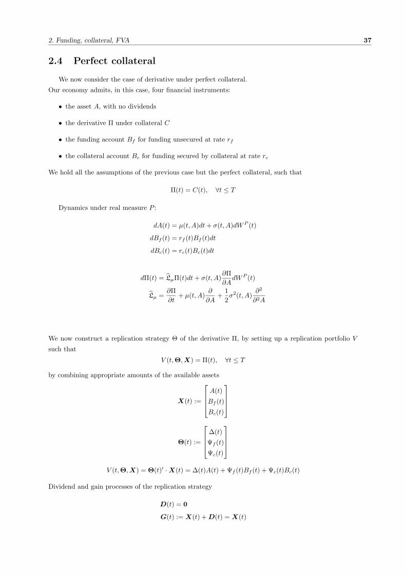
2.4 Perfect collateral
We now consider the case of derivative under perfect collateral.
Our economy admits, in this case, four financial instruments:
• the asset A, with no dividends
• the derivative Π under collateral C
• the funding account Bf for funding unsecured at rate rf
• the collateral account Bc for funding secured by collateral at rate rc
We hold all the assumptions of the previous case but the perfect collateral, such that
Π(t) = C(t), ∀t ≤ T
Dynamics under real measure P :
dA(t) = µ(t, A)dt+ σ(t, A)dWP (t)
dBf (t) = rf (t)Bf (t)dt
dBc(t) = rc(t)Bc(t)dt
dΠ(t) = LµΠ(t)dt+ σ(t, A)∂Π
∂AdWP (t)
Lµ =∂Π
∂t+ µ(t, A)
∂
∂A+
1
2σ2(t, A)
∂2
∂2A
We now construct a replication strategy Θ of the derivative Π, by setting up a replication portfolio V
such that
V (t,Θ,X) = Π(t), ∀t ≤ T
by combining appropriate amounts of the available assets
X(t) :=
A(t)
Bf (t)
Bc(t)
Θ(t) :=
∆(t)
Ψf (t)
Ψc(t)
V (t,Θ,X) = Θ(t)′ ·X(t) = ∆(t)A(t) + Ψf (t)Bf (t) + Ψc(t)Bc(t)
Dividend and gain processes of the replication strategy
D(t) = 0
G(t) := X(t) +D(t) = X(t)
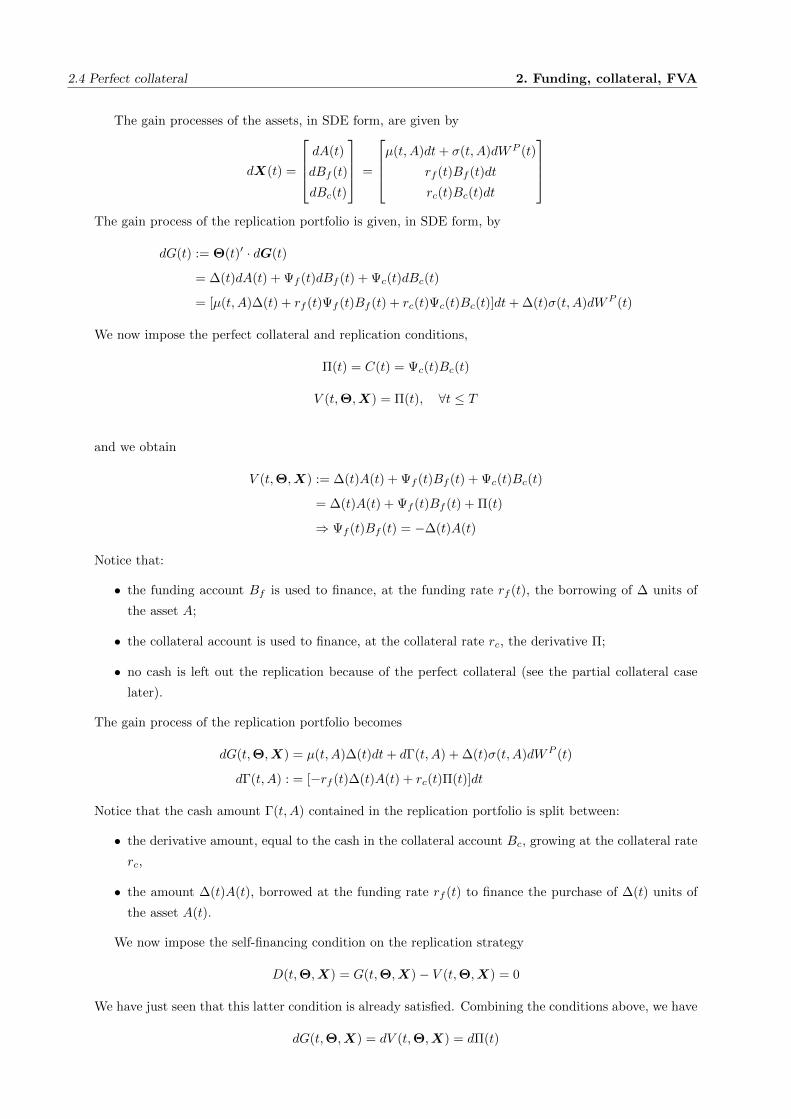
2.4 Perfect collateral 2. Funding, collateral, FVA
The gain processes of the assets, in SDE form, are given by
dX(t) =
dA(t)
dBf (t)
dBc(t)
=
µ(t, A)dt+ σ(t, A)dWP (t)
rf (t)Bf (t)dt
rc(t)Bc(t)dt
The gain process of the replication portfolio is given, in SDE form, by
dG(t) := Θ(t)′ · dG(t)
= ∆(t)dA(t) + Ψf (t)dBf (t) + Ψc(t)dBc(t)
= [µ(t, A)∆(t) + rf (t)Ψf (t)Bf (t) + rc(t)Ψc(t)Bc(t)]dt+ ∆(t)σ(t, A)dWP (t)
We now impose the perfect collateral and replication conditions,
Π(t) = C(t) = Ψc(t)Bc(t)
V (t,Θ,X) = Π(t), ∀t ≤ T
and we obtain
V (t,Θ,X) := ∆(t)A(t) + Ψf (t)Bf (t) + Ψc(t)Bc(t)
= ∆(t)A(t) + Ψf (t)Bf (t) + Π(t)
⇒ Ψf (t)Bf (t) = −∆(t)A(t)
Notice that:
• the funding account Bf is used to finance, at the funding rate rf (t), the borrowing of ∆ units of
the asset A;
• the collateral account is used to finance, at the collateral rate rc, the derivative Π;
• no cash is left out the replication because of the perfect collateral (see the partial collateral case
later).
The gain process of the replication portfolio becomes
dG(t,Θ,X) = µ(t, A)∆(t)dt+ dΓ(t, A) + ∆(t)σ(t, A)dWP (t)
dΓ(t, A) : = [−rf (t)∆(t)A(t) + rc(t)Π(t)]dt
Notice that the cash amount Γ(t, A) contained in the replication portfolio is split between:
• the derivative amount, equal to the cash in the collateral account Bc, growing at the collateral rate
rc,
• the amount ∆(t)A(t), borrowed at the funding rate rf (t) to finance the purchase of ∆(t) units of
the asset A(t).
We now impose the self-financing condition on the replication strategy
D(t,Θ,X) = G(t,Θ,X)− V (t,Θ,X) = 0
We have just seen that this latter condition is already satisfied. Combining the conditions above, we have
dG(t,Θ,X) = dV (t,Θ,X) = dΠ(t)

2. Funding, collateral, FVA 39
Introducing in this latter equation the expressions of dG(t,Θ,X) and dΠ(t) obtained before, and rear-
ranging terms we obtain the SDE
[∂Π
∂t+ µ(t, A)
(∂Π
∂A−∆(t)
)+
1
2σ2(t, A)
∂2Π
∂2A
]dt+ σ(t, A)
(∂Π
∂A−∆(t)
)dWP (t) = dΓ(t, A)
We finally impose the risk neutral condition ∆(t) = ∂Π∂A , such that the stochastic (risky) term with
dWP (t) disappears, and we obtain a generalised Black-Scholes PDE equation for the derivative’s
price Π(t, A)
LrfΠ(t) = rc(t)Π(t)
Lrf :=∂
∂t+ rf (t)A(t)
∂
∂A+
1
2σ2(t, A)
∂2
∂2A
Using the Feynman-Kac theorem we may switch from the PDE representation to the SDE representation
given by
Π(t) = EQt [Dc(t;T )Π(T )] (2.4.1)
Dc(t;T ) := exp
[−∫ T
t
rc(u)du
](2.4.2)
dA(t) = rf (t)A(t)dt+ σ(t, A)dWQ(t) (2.4.3)
We conclude that we discount at the collateral rate.
Remark 2.7. 1. Funding measure:
the probability measure Q introduced via Feynman-Kac is associated with the risk neutral drift rf
appearing in the SDE dynamics of the asset A. It is the same measure of the uncollateralised case,
but now the numeraire is the collateral account Bc.
2. Borrowing/lending return:
we notice that, over the time interval [t, t + dt), the derivative Π(t) and the cash flow rc(t)Π(t)dt
generated by the (perfect) collateral margination, are equivalent to a derivative Π(t) without col-
lateral but with a continuous dividend yield rc(t)Π(t)dt, such that rf − rc the rate is the actual
(instantaneous) borrowing/lending cost/return including the collateral.
3. Zero Coupon Bonds:
we can define secured (collateralized) Zero Coupon Bonds, such that
Pc(T ;T ) = 1
Pc(t;T ) = EQt [Dc(t;T )]
4. T -Forward measure:
we can switch from the funding measure associated with numeraire Bc(t) to T -forward measure
Q ⊂ T associated with secured (collateralised) numeraire Pc(t;T ) using the corresponding Radon-

2.4 Perfect collateral 2. Funding, collateral, FVA
Nikodym derivative as follows
Mc(t, T ) =Pc(t;T )
Bc(t)
Πc(t) = EQt [Dc(t;T )Π(T )]
= M(t, T )EQTc
t
[Dc(t;T )
M(T, T )Π(T )
]= Pc(t;T )EQ
Tc
t
[1
Pc(T, T )Π(T )
]= Pc(t;T )EQ
Tc
t [Π(T )]
We remember that any positive martingale process (not necessary the ratio between two numeraires)
can be used as Radon-Nikodym derivative in a measure change.
5. (Im)perfect collateral:
Since real CSAs are far from being perfect, a more general proof is required to take into account
imperfect collateral, such that Bc(t) 6= Π(t), also in terms of different currencies.
6. Equity asset:
The lending/borrowing of some assets is often realised through repo contracts and funded at the
repo rate. Furthermore, assets may pay, in general, dividends. Typical example is equity asset.
Thus a more general proof is necessary to deal with these special case.
7. Funding Valuation Adjustment (FVA):
Comparing the collateralised vs uncollateralised prices we can define a Funding Value Adjustment
(FVA) such that, in additive form,
Πf (t) = EQt [Df (t;T )Π(T )]
= EQt[Df (t;T )
Dc(t;T )Dc(t;T )Π(T )
]= EQt [Dc(t;T )Π(T )] + FV Af,c(t)
= Πc(t) + FV Af,c(t)
FV Af,c : = Πf (t)−Πc(t)
The calculation of the FVA above depends on the correlated dynamics of the funding and collateral
rates, and is thus model dependent. If the variance of the ratio between the funding and the
collateral (stochastic) discounts is negligible with respect to the variance of the remaining discounted
payoff 1,
V ar
[Df (t;T )
Dc(t;T )
] V ar[Dc(t;T )Π(T )]
we may write
Πf (t) = EQt[Df (t;T )
Dc(t;T )Dc(t;T )Π(T )
]∼= EQt
[Df (t;T )
Dc(t;T )
]EQt [Dc(t;T )Π(T )]
= EQt[Df (t;T )
Dc(t;T )
]Πc(t)
FV Af,c(t) ∼=EQt[Df (t;T )
Dc(t;T )
]− 1
Πc(t)
1This condition is less restrictive than the deterministic basis limit used below.

2. Funding, collateral, FVA 41
In the limit of deterministic basis we obtain the simple expression
EQt[Df (t;T )
Dc(t;T )
]∼=
EQt [Df (t;T )]
EQt [Dc(t;T )]=Pf (t;T )
Pc(t;T )= e−
∫ Ttsf,c(u)du
FV Af,c ∼=[e−
∫ Ttsf,c(u)du − 1
]Πc(t) ∼= −
[∫ T
t
sf,c(u)du
]Πc(t)
sf,c(t) := rf (t)− rc(t)
2.5 Perfect collateral for derivative and hedge
We now consider the special case of perfect collateral, in which also the asset A is perfectly collater-
alized, with its distinct collateral rate.
In this case our economy admits, four financial instruments:
• the asset A under collateral CA
• the derivative Π under collateral CΠ
• the derivatives’ collateral account BcΠ for funding Π secured by collateral at rate rcΠ
• the asset’s collateral account BcA for funding A secured by collateral at rate rcA
The proof follows the previous case of perfect collateral, with the substitutions
Bf → BcA, rf → rcA
Bc → BcΠ, rc → rcΠ
C → CΠ
We obtain the PDE
LrcAΠ(t) = rcΠ(t)Π(t)
LrcA :=∂
∂t+ rcA(t)A(t)
∂
∂A+
1
2σ2(t, A)
∂2
∂2A
Using the Feynman-Kac
Π(t) = EQt [DcΠ(t;T )Π(T )]
DcΠ(t;T ) := exp
[−∫ T
t
rcΠ(u)du
]dA(t) = rcA(t)A(t)dt+ σ(t, A)dWQ(t)
We conclude that, in case of perfect collateral for both the derivative and the hedge, the stochastic process
for the asset A is driven by the collateral rate rcA associated with the asset A.

2.6 Perfect collateral, dividends, repo 2. Funding, collateral, FVA
2.6 Perfect collateral, dividends, repo
We now consider the case of derivatives on a dividend paying asset A subject to repo funding. In
practice, the asset A, instead of being traded directly, funded through an unsecured funding account Bf
at the funding rate rf , is traded indirectly through repo contracts, secured by the asset A and funded at
the repo rate rR.
Hence, our economy admits, in this case, four financial instruments:
• the asset A, and its dividends at rate rD
• the derivative Π under collateral C
• the collateral account Bc for funding secured by collateral at rate rc
• the repo contract ΠR(A) for funding secured by asset A at repo rate rR
Dynamics under real measure P :
dA(t) = µ(t, A)dt+ σ(t, A)dWP (t)
dBc(t) = rc(t)Bc(t)dt
dΠ(t) = LµΠ(t)dt+ σ(t, A)∂Π
∂AdWP (t)
Lµ =∂
∂t+ µ(t, A)
∂
∂A+
1
2σ2(t, A)
∂2
∂2A
Regarding the repo contract dynamics, we must remember that, for the repo holder:
• there is a continuous positive cash flow of dividends +rD(t)A(t)dt
• there is a continuous negative cash flow of repo interests −rR(t)A(t)dt,
• the price is linearly dependent on the asset A
Thus, using Ito’s Lemma, we obtain
dΠR(t) =∂ΠR
∂tdt+
∂ΠR
∂AdA(t) +
1
2
∂2ΠR
∂2AdA2(t) + rD(t)A(t)dt− rR(t)A(t)dt
= dA(t) + [rD(t)− rR(t)]A(t)dt
(We have considered unit nominal).
The replication strategy of the derivative Π is obtained by combining appropriate amounts [∆, Ψ] of
the available assets [ΠR, Bc]
X(t) :=
[0
Bc(t)
]
Θ(t) :=
[∆(t)
Ψc(t)
]where we have taken into account that the repo contract is always traded at par on the market, such
that ΠR(t) = 0 for time t trading.
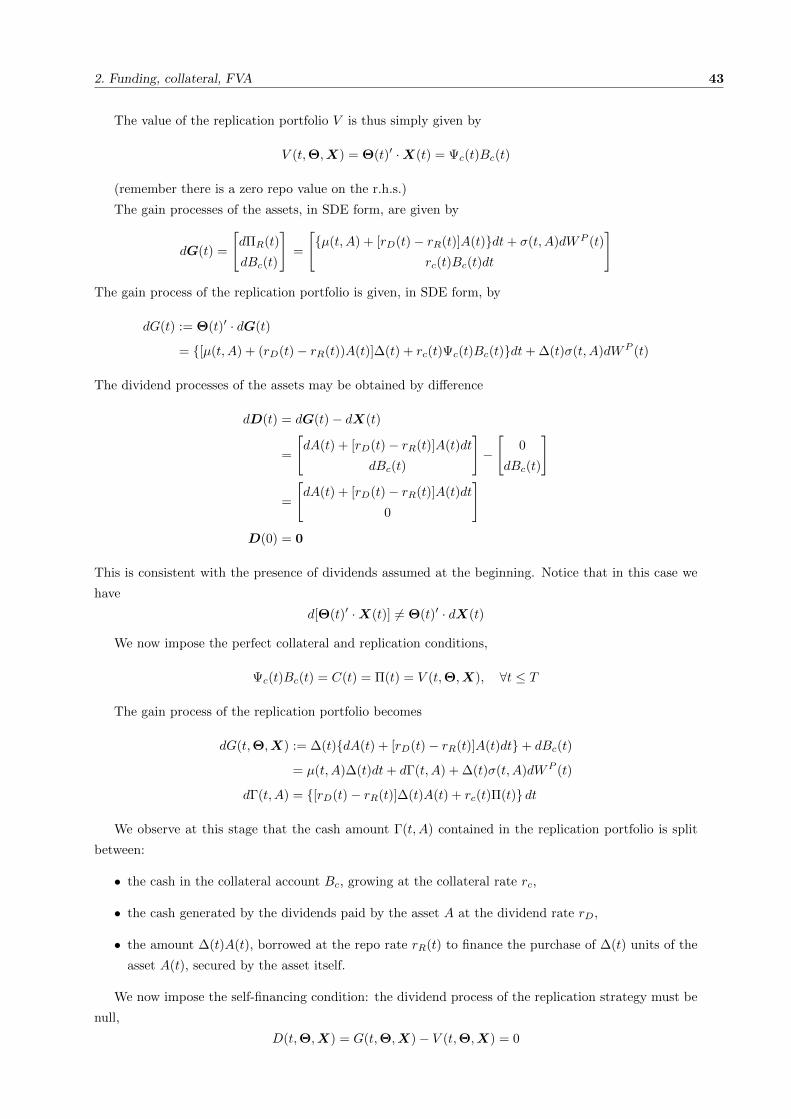
2. Funding, collateral, FVA 43
The value of the replication portfolio V is thus simply given by
V (t,Θ,X) = Θ(t)′ ·X(t) = Ψc(t)Bc(t)
(remember there is a zero repo value on the r.h.s.)
The gain processes of the assets, in SDE form, are given by
dG(t) =
[dΠR(t)
dBc(t)
]=
[µ(t, A) + [rD(t)− rR(t)]A(t)dt+ σ(t, A)dWP (t)
rc(t)Bc(t)dt
]
The gain process of the replication portfolio is given, in SDE form, by
dG(t) := Θ(t)′ · dG(t)
= [µ(t, A) + (rD(t)− rR(t))A(t)]∆(t) + rc(t)Ψc(t)Bc(t)dt+ ∆(t)σ(t, A)dWP (t)
The dividend processes of the assets may be obtained by difference
dD(t) = dG(t)− dX(t)
=
[dA(t) + [rD(t)− rR(t)]A(t)dt
dBc(t)
]−
[0
dBc(t)
]
=
[dA(t) + [rD(t)− rR(t)]A(t)dt
0
]D(0) = 0
This is consistent with the presence of dividends assumed at the beginning. Notice that in this case we
have
d[Θ(t)′ ·X(t)] 6= Θ(t)′ · dX(t)
We now impose the perfect collateral and replication conditions,
Ψc(t)Bc(t) = C(t) = Π(t) = V (t,Θ,X), ∀t ≤ T
The gain process of the replication portfolio becomes
dG(t,Θ,X) := ∆(t)dA(t) + [rD(t)− rR(t)]A(t)dt+ dBc(t)
= µ(t, A)∆(t)dt+ dΓ(t, A) + ∆(t)σ(t, A)dWP (t)
dΓ(t, A) = [rD(t)− rR(t)]∆(t)A(t) + rc(t)Π(t) dt
We observe at this stage that the cash amount Γ(t, A) contained in the replication portfolio is split
between:
• the cash in the collateral account Bc, growing at the collateral rate rc,
• the cash generated by the dividends paid by the asset A at the dividend rate rD,
• the amount ∆(t)A(t), borrowed at the repo rate rR(t) to finance the purchase of ∆(t) units of the
asset A(t), secured by the asset itself.
We now impose the self-financing condition: the dividend process of the replication strategy must be
null,
D(t,Θ,X) = G(t,Θ,X)− V (t,Θ,X) = 0
2.7 Partial collateral 2. Funding, collateral, FVA
⇒ dG(t,Θ,X) = dV (t,Θ,X) = dΠ(t).
Introducing the gain process of the strategy on the l.h.s, the derivative process on the r.h.s of the
previous equation, and rearranging terms we obtain the SDE
∂Π
∂t+ µ(t, A)
[∂Π
∂A−∆(t)
]+
1
2σ2(t, A)
∂2Π
∂2A
]dt+ σ(t, A)
[∂Π
∂A−∆(t)
]dWP (t) = dΓ(t, A)
We finally impose the risk neutral condition ∆(t) = ∂Π∂A , such that the stochastic (risky) term with
dWP (t) disappears, and we obtain a generalised Black-Scholes equation for the derivative’s price Π(t)
LrR−rDΠ(t) = rc(t)Π(t)
LrR−rD :=∂
∂t+ (rR(t)− rD(t))A(t)
∂
∂A+
1
2σ2(t, A)
∂2
∂2A
Using the Feynman-Kac theorem we may switch from the PDE representation to the SDE representation
given by
Π(t) = EQt [Dc(t;T )Π(T )]
Dc(t;T ) := exp
[−∫ T
t
rc(u)du
]dA(t) = [rR(t)− rD(t)]A(t)dt+ σ(t, A)dWQ(t)
We conclude that we discount at the collateral rate.
Remark 2.8. 1. Funding measure:
the probability measure Q introduced via Feynman-Kac is associated with the risk neutral drift rR
appearing in the SDE dynamics of the asset A. It is the same measure of the collateralised case,
with numeraire the collateral account Bc.
2. Risk neutral drift:
The repo rate rR is the correct rate to be used in the risk neutral dynamics of assets subject to
repo. We may think that the repo (short) rate rR(t) is associated with a repo account BR, such
that
dBR(t) = rR(t)BR(t)dt
The repo rate, being associated with a secured transaction, may be considered a good proxy of a
risk free rate. In practice, overnight repos are close to unsecured overnight rates.
3. Funding Valuation Adjustment (FVA):
The price Π(t) is different from the no repo case, because of the different risk neutral drift in the
SDE dynamics of the asset A. According to the consideration above, the difference is small. We
conclude that FVA is negligible.
2.7 Partial collateral
We now relax the hypothesis of perfect collateral and consider the more general case of partial collat-
eral C(t) 6= Π(t), in the same currency of the derivative.

2. Funding, collateral, FVA 45
Our economy admits, in this case, four financial instruments:
• the asset A
• the derivative Π under partial collateral C
• the funding account Bf for funding unsecured at rate rf
• the collateral account Bc for funding secured by collateral at rate rc
In general, we may assume the following dynamics under the real measure P :
dA(t) = µ(t, A)dt+ σ(t, A)dWP (t)
dBf (t) = rf (t)Bf (t)dt
dBc(t) = rc(t)Bc(t)dt
dΠ(t) = LµΠ(t)dt+ σ(t, A)∂Π
∂AdWP (t)
Lµ =∂
∂t+ µ(t, A)
∂
∂A+
1
2σ2(t, A)
∂2
∂2A
The replication strategy of the derivative Π is obtained by combining appropriate amounts Θ of the
available assets
X(t) :=
A(t)
Bf (t)
Bc(t)
Θ(t) :=
∆(t)
Ψf (t)
Ψc(t)
The value of the replication portfolio V is thus simply given by
V (t,Θ,X) = Θ(t)′ ·X(t) = ∆(t)A(t) + Ψf (t)Bf (t) + Ψc(t)Bc(t)
The gain and dividend processes of the assets, in SDE form, are given directly by the dynamics
discussed before, as
dG(t) : =
dA(t)
dBf (t)
dBc(t)
=
µ(t, A)dt+ σ(t, A)dWP (t)
rf (t)Bf (t)dt
rc(t)Bc(t)dt
dD(t) = 0
The gain process of the replication portfolio is given, in SDE form, by
dG(t) := Θ(t)′ · dG(t)
= µ(t, A)∆(t) + rf (t)Ψf (t)Bf (t) + rc(t)Ψc(t)Bc(t)dt+ ∆(t)σ(t, A)dWP (t)
We now impose the perfect collateral and replication conditions,
V (t,Θ,X) = Π(t) = ∆(t)A(t) + Ψf (t)Bf (t) + Ψc(t)Bc(t), ∀t ≤ T

2.7 Partial collateral 2. Funding, collateral, FVA
⇒ Ψf (t)Bf (t) = Π(t)−Ψc(t)Bc(t) = Π(t)−∆(t)A(t)− C(t)
consistently with the fact that the funding account Bf is used to finance the borrowing of ∆(t) units of
the asset A(t) at the funding rate rf (t).
The gain process of the replication portfolio becomes
dG(t,Θ,X) = µ(t, A)∆(t)dt+ dΓ(t, A) + ∆(t)σ(t, A)dWP (t)
dΓ(t, A) = −rf (t)∆(t)A(t) + rf (t)Π(t)− [rf (t)− rc(t)]C(t)dt
= −rf (t)∆(t)A(t) + rc(t)C(t)− rf (t)[Π(t)− C(t)]dt
We observe that the cash amount Γ(t, A) in the replication portfolio is split between:
• the collateral C, growing at the collateral rate rc,
• the amount ∆(t)A(t), borrowed at the funding rate rf (t) to finance the purchase of ∆(t) units of
the asset A(t),
• the off-collateral amount Π(t)− C(t), borrowed/lent at the funding rate rf (t)
We now impose the self-financing condition: the dividend process of the replication strategy must be
null,
D(t,Θ,X) = G(t,Θ,X)− V (t,Θ,X) = 0
⇒ dG(t,Θ,X) = dV (t,Θ,X) = dΠ(t).
Introducing, in the previous equation, the gain process of the replication portfolio on the l.h.s, the
derivative process on the r.h.s, and rearranging terms, we have
∂Π
∂t+ µ(t, A)
[∂Π
∂A−∆(t)
]+
1
2σ2(t, A)
∂2Π
∂2A
]dt+ σ(t, A)
[∂Π
∂A−∆(t)
]dWP (t) = dΓ(t, A)
Finally, we impose the risk neutral condition ∆(t) = ∂Π∂A and we obtain a generalised Black-Scholes
equation for the derivative’s price Π(t)
LrfΠ(t) = rf (t)Π(t)− [rf (t)− rc(t)]C(t)
Lrf :=∂
∂t+ (rf (t))A(t)
∂
∂A+
1
2σ2(t, A)
∂2
∂2A
Using the Feynman-Kac theorem we obtain the SDE representation
Π(t) = EQt
[Dc(t;T )Π(T ) +
∫ T
t
Dc(t;u)[rf (u)− rc(u)][Π(u)− C(u)]du
]
Dc(t;T ) := exp
[−∫ T
t
rc(u)du
]dA(t) = rf (t)A(t)dt+ σ(t, A)dWQ(t)
Remark 2.9. Funding Value Adjustment (FVA)
We may rewrite the previous formula as follows
Πf,c(t) = EQt
[Dc(t;T )Π(T ) +
∫ T
t
Dc(t;u)[rf (u)− rc(u)][Πf,c(u)− C(u)]du
]= Πc(t) + FV Af,c(t)
FV Af,c : = Πf,c(t)−Πc(t)
= EQt
[∫ T
t
Dc(t;u)[rf (u)− rc(u)][Πf,c(u)− C(u)]du
]

2. Funding, collateral, FVA 47
In this case, the FVA amounts to the expected difference between the trade and collateral values, weighted
with the difference between funding and collateral rates, integrated over the residual life of the trade.
2.8 Perfect collateral, stochastic rates
We consider now the case of stochastic funding rates with perfect collateral. Stochastic funding means
that funding rates are stochastic, there are more risk factors to hedge.
Our economy admits, in this case, six financial instruments:
• the asset A,
• the uncollateralized asset Af , e.g. a zero coupon bond Pf (t, s)
• the collateralized asset Ac, e.g. a zero coupon bond Pc(t, s)
• the derivative Π under perfect collateral C
• the funding account Bf for funding unsecured at rate rf
• the collateral account Bc for funding secured by collateral at rate rc
Notice that:
• Non tradable assets, such as interest rates, inflation, fx, etc. can’t appear directly as hedging
instruments, but through some corresponding tradable financial instruments. In particular, funding
rates rx may enter in the form of Zero Coupon Bonds, Ax(t) = Px(t, s).
• Additional financial instruments associated with (stochastic) funding rates are required to hedge
the additional risk factors.
In general, we may assume the following dynamics under the real measure P :
dA(t) = µA(t, A)dt+ σA(t, A)dW P (t)
dAx(t) = µx(t, Ax)dt+ σx(t, Ax)dW P (t)
dBx(t) = rx(t)Bx(t)dt
dΠ(t) = LµΠ(t)dt+
[∂Π
∂AσA(t, A) +
∂Π
∂Afσf (t, Af ) +
∂Π
∂Acσc(t, Ac)
]· dW P (t)
Lµ : =∂
∂t+ µA(t, A)
∂
∂A+ µf (t, Af )
∂
∂Af+ µc(t, Ac)
∂
∂Ac+
1
2Σ2(t, A,Af , Ac)(t) ·
∂2
∂2A
Σ2(t, A,Af , Ac) ·∂2
∂2A: = σ2
A(t, A)∂2
∂2A+ σ2
f (t, Af )∂2
∂2Af+ σ2
c(t, Ac)∂2
∂2Ac+
+ σA(t, A) ·[σ2f (t, Af )
∂2
∂A∂Af+ σ2
c(t, Ac)∂2
∂A∂Ac
]+ σf (t, Af ) · σc(t, Ac)
∂2
∂Af∂Ac
dWPi (t)dWP
j (t) = δi,jdt
x : = f, c
The replication strategy of the derivative Π is obtained by combining appropriate amounts Θ of the
available assets

2.8 Perfect collateral, stochastic rates 2. Funding, collateral, FVA
X(t) :=
A(t)
Af (t)
Ac(t)
Bf (t)
Bc(t)
Θ(t) :=
∆A(t)
∆f (t)
∆c(t)
Ψf (t)
Ψc(t)
The value of the replication portfolio V is thus simply given by
V (t,Θ,X) = Θ(t)′ ·X(t) = ∆A(t)A(t) + ∆f (t)Af (t) + ∆c(t)Ac(t) + Ψf (t)Bf (t) + Ψc(t)Bc(t)
The gain and dividend processes of the assets, in SDE form, are given directly by the dynamics
discussed before, as
dG(t) : =
dA(t)
dAf (t)
dAc(t)
dBf (t)
dBc(t)
=
µA(t, A)dt+ σA(t, A) · dW P (t)
µf (t, Af )dt+ σf (t, Af ) · dW P (t)
µc(t, Ac)dt+ σc(t, Ac) · dW P (t)
rf (t)Bf (t)dt
rc(t)Bc(t)dt
dD(t) = 0
The gain process of the replication portfolio is given, in SDE form, by
dG(t) := Θ(t)′ · dG(t)
= µA(t, A)∆A(t) + µf (t, Af )∆f (t) + µc(t, Ac)∆c(t) + rf (t)Ψf (t)Bf (t) + rc(t)Ψc(t)Bc(t)dt+
+ [∆A(t)σA(t, A) + ∆f (t)σf (t, Af ) + ∆c(t)σc(t, Ac)]dWP (t)
We now impose the perfect collateral and replication conditions,
V (t,Θ,X) = Π(t)
= ∆A(t)A(t) + ∆f (t)Af (t) + ∆c(t)Ac(t) + Ψf (t)Bf (t) + Ψc(t)Bc(t)
= ∆A(t)A(t) + ∆f (t)Af (t) + Ψf (t)Bf (t) + Π(t)
where we have used the generalised perfect collateral condition
Π(t) = C(t) = Ψc(t)Bc(t) + ∆(t)Ac(t)
Thus we obtain the generalised unsecured funding condition
Ψf (t)Bf (t) = −∆A(t)A(t)−∆f (t)Af (t)
consistently with the fact that the funding account Bf is used to finance the borrowing of ∆A(t) units of
the asset A(t) and ∆f (t) units of the asset Af (t) at the funding rate rf (t).
2. Funding, collateral, FVA 49
The gain process of the replication portfolio becomes
dG(t,Θ,X) = dΠ(t) = LµΠ(t)dt =
= [µA(t, A)∆A(t) + µf (t, Af )∆f (t) + µc(t, Ac)∆c(t)]dt+
+ dΓ(t, A,Af , Ac)+
+ [∆A(t)σA(t, A) + ∆f (t)σf (t, Af ) + ∆c(t)σc(t, Ac)] · dW P (t)
dΓ(t, A) = −rf (t)[∆A(t)A(t) + ∆f (t)Af (t)] + rc(t)[Π(t)−∆c(t)Ac(t)]dt
We observe that the cash amount Γ(t, A) in the replication portfolio is split between:
• the collateral amount C(t) = Π−∆c(t)Ac(t), growing at the collateral rate rc,
• the amount ∆(t)A(t), borrowed at the funding rate rf (t) to finance the purchase of ∆(t) units of
the asset A(t), and ∆f (t) units of the asset Af (t).
We now impose the self-financing condition: the dividend process of the replication strategy must be
null,
D(t,Θ,X) = G(t,Θ,X)− V (t,Θ,X) = 0
⇒ dG(t,Θ,X) = dV (t,Θ,X) = dΠ(t).
Introducing, in the previous equation, the gain process of the replication portfolio on the l.h.s, the
derivative process on the r.h.s, and rearranging terms, we have∂Π
∂t+ µA(t, A)
[∂Π
∂A−∆A(t)
]+ µf (t, Af )
[∂Π
∂Af−∆f (t)
]+ µc(t, Ac)
[∂Π
∂Ac−∆c(t)
]+
1
2Σ2(t, A,Af , Ac)
∂2Π
∂2A
dt+
[∂Π
∂A−∆A(t)
]σA(t, A) +
[∂Π
∂Af−∆f (t)
]σf (t, Af )+
+
[∂Π
∂Ac−∆c(t)
]σc(t, Ac)
· dW P (t) = dΓ(t, A,Af , Ac)
Finally, imposing the generalised risk neutral condition
∆A(t) =∂Π
∂A∆f (t) =
∂Π
∂Af∆c(t) =
∂Π
∂Ac
we obtain a generalised Black-Scholes PDE equation for the derivative’s price Π(t)
Lf,cΠ(t) = rc(t)Π(t)
Lf,c :=∂
∂t+ rf (t)
[A(t)
∂
∂A+Af (t)
∂
∂Af
]+ rc(t)Ac(t)
∂
∂Ac
1
2Σ2(t, A,Af , Ac) ·
∂2
∂2A
Using the Feynman-Kac theorem we obtain the SDE representation
Π(t) = EQt [Dc(t;T )Π(T )]
Dc(t;T ) := exp
[−∫ T
t
rc(u)du
]dA(t) = rf (t)A(t)dt+ σA(t, A) · dWQ(t)
dAx(t) = rx(t)Ax(t)dt+ σx(t, Ax) · dWQ(t)
We conclude that we discount at the collateral rate.

2.9 General case 2. Funding, collateral, FVA
Remark 2.10. IR dynamics
In the risk neutral measure the dynamics of the stochastic rates rx is expressed via the functional de-
pendence on the instruments Ax. We could proceed the other way around, postulating from the very
beginning, stochastic process of the rates in the risk-neutral measure.
This freedom allows to select their dynamics with appropriate characteristics that can be calibrated to
the corresponding yield curves. For example, we could choose the Hull-White dynamics such that, under
the risk neutral measure Q ,
drx(t) = [kx(t)− ax(t)rx(t)]dt+ σrx(t) · dWQ(t)
Remark 2.11. IR instruments
Next, we can specify the interest rate instruments Ax used in the replication. One possible choice
are unsecured and (perfectly) collateralised zero coupon bonds, Ax(t) = Px(t, T ′), with some maturity
T ′ > T .
The parameters kx(t) in the Hull-White dynamics above can be calibrated to the market zero coupon
bond curves. Using Ito’s lemma we obtain the price dynamics of the zero coupon bonds as
dPx(t, T ′) = rx(t)Px(t, T ′)dt− Px(t, T ′)σPx(t, T ′) · dWQ(t)
σPx(t, T ′) = σrx(t)
∫ T ′
t
e−∫ utax(v)dvdu
x = f, c
Notice that the zero coupon bonds dynamics inherit appropriate drifts corresponding to their underlying
(short) rates rx.
2.9 General case
We now consider the more general case of multiple assets A, multiple stochastic funding rates rx,
dividends and partial collateral.
Our economy admits, in this case, multiple financial instruments: the vector of assetsAx = [Af , Ac, AR]
according to the funding of their associated hedging strategies (unsecured, collateral, repo) the derivative
Π on assets Ax under partial CSA the vector of funding accounts Bx = [Bf , Bc, BR] with funding rates
rx = [rf , rc, rR] The generalised funding conditions become
∆f (t)Af (t) + Ψf (t)Bf (t) = Π(t)− CΠ(t)
∆c(t)Ac(t) + Ψc(t)Bc(t) = CΠ(t)
∆R(t)AR(t) + ΨR(t)BR(t) = 0
We obtain a generalised Black-Scholes PDE equation for the derivative’s price Π(t)
LrΠ(t) = rf (t)Π(t)− [rf (t)− rc(t)]CΠ(t)
Lr =∂
∂t+∑x
[rx(t)− rD(t)]Ax(t) · ∂
∂Ax+
1
2
∑x,y
σx(t,Ax) · σy(t,Ay) · ∂2
∂Ax∂Ay
and, using Feynman-Kac, the SDE representation
Π(t) = EQt
[Dc(t;T )Π(T )−
∫ T
t
Dc(u, T )[rf (u)− rc(u)][Π(u)− CΠ(u)]du
]

2. Funding, collateral, FVA 51
Dx(t;T ) := exp
[−∫ T
t
rx(u)du
]dAx(t) = [rx(t)− rD(t)]Ax(t)dt+ σx(t,Ax) · dWQ(t)
2.10 Multiple currency
We consider now the case of different currency for the derivative and its funding.
Our economy admits, in this case, five financial instruments:
• the asset Aα, in currency α, with no dividends
• the derivative Πα under partial collateral Cβ in currency β
• the funding account Bαf for funding unsecured in currency α at rate rαf
• the funding account Bβf for funding unsecured in currency β at rate rβf
• the collateral account Bβc for funding secured by collateral Cβ at rate rβc
We also assume that the derivative Π is under perfect collateral, such that
Πα(t) = xαβ(t)Cβ(t), ∀t ≤ T
where xαβ is the spot exchange rate expressing the value in currency α of one unit of currency β.
We have the following dynamics under the real measure Pα:
dAα(t) = µ(t, Aα)dt+ σ(t, Aα)dWP,α(t)
dBαf (t) = rαf (t)Bαf (t)dt
dBβf (t) = rβf (t)Bβf (t)dt
dBβc (t) = rβc (t)Bβc (t)dt
dΠα(t) =
[∂Πα
∂t+ µ(t, Aα)
∂Π
∂A+
1
2σ2(t, Aα)
∂2Πα
∂2A
]dt+ σ2(t, Aα)
∂Π
∂AdWP,α(t)
We now construct the replication strategy of the derivative Πα by setting up a replication portfolio
V α such that
V α(t,Θ,X) = Πα(t), ∀t ≤ T
by combining appropriate amounts Θ of the available assets X
X(t) :=
Aα(t)
Bαf (t)
Bβf (t)
Bβc (t)
Θ(t) :=
∆(t)
Ψαf (t)
Ψβf (t)xαβ(t)
Ψβc (t)xαβ(t)

2.10 Multiple currency 2. Funding, collateral, FVA
The value of the replication portfolio V α(t,Θ,X) is given by
V (t,Θ,X) = Θ(t)′ ·X(t) = ∆(t)Aα(t) + Ψαf (t)Bαf (t) + Ψβ
f (t)xαβ(t)Bβf (t) + Ψβc (t)xαβ(t)Bc(t)
The gain and dividend processes of the assets, in SDE form, are given directly by the dynamics
discussed before, as
dG(t) : =
dAα(t)
dBαf (t)
dBβf (t)
dBβc (t)
=
µ(t, Aα)dt+ σ(t, Aα)dWP,α(t)
rαf (t)Bαf (t)dt
rβf (t)Bβf (t)dt
rβc (t)Bβc (t)dt
dD(t) = 0
dG(t) = dX(t)
We now impose the perfect collateral and replication conditions, and we obtain
V α(t,Θ,X) = ∆(t)Aα(t) + Ψαf (t)Bαf (t) + Ψβ
f (t)xαβ(t)Bβf (t) + Ψβc (t)xαβ(t)Bβc (t)
= ∆(t)Aα(t) + Ψαf (t)Bαf (t) + Ψβ
f (t)xαβ(t)Bβf (t) + Π(t)
V α(t,Θ,X) = Πα, ∀t ≤ T
⇒ Ψαf (t)Bαf (t) = −∆(t)Aα(t)−Ψβ
f (t)xαβ(t)Bβf (t)
consistently with the fact that the funding account Bαf is used to finance, in currency α the borrowing
of ∆(t) units of the asset Aα(t) and Ψf (t)xαβ(t) units of cash Bβf (t) in currency β, at the funding rate
rαf (t).
The gain process of the replication portfolio, in SDE form, is given by
dGα(t,Θ,X) = dXα(t,Θ,X) = Θ(t)′ · dG(t)
= µ(t, Aα)∆(t)dt+ dΓα(t, Aα) + ∆(t)σ(t, Aα)dWP,α(t)
dΓα(t, Aα) : =− rαf (t)∆(t)Aα(t) +
[rβf (t)− rαf (t)
]Ψβf (t)xαβ(t)Bβf (t) + rβc (t)Πα(t)
dt
=− rαf (t)∆(t)Aα(t) +
[rβc (t) + rβf (t)− rαf (t)
]Πα(t)
dt
where we have chosen Ψβfx
αβBβf (t) = Πα(t), such that Ψβfx
αβBβf (t) units of cash Bβf (t) are used to
fund the derivative Πα(t).
We observe that the cash amount Γα(t) in the replication portfolio is split between:
• the amount ∆(t)Aα(t) in currency α, borrowed at the funding rate rαf (t) to finance the purchase of
∆(t) units of the asset Aα(t),
• the amount Bβc (t) in the collateral account (currency β), growing at the cross currency collateral
rate rβc (t) + rβf (t)− rαf
We now impose the self-financing condition: the dividend process of the replication strategy must be
null,
Dα(t,Θ,X) = Gα(t,Θ,X)− V α(t,Θ,X) = 0
⇒ dGα(t,Θ,X) = dV α(t,Θ,X) = dΠα(t).
Introducing, in the previous equation, the gain process of the replication portfolio on the l.h.s, the
derivative process on the r.h.s, and rearranging terms, we have
2. Funding, collateral, FVA 53
∂Πα
∂t+ µ(t, Aα)
[∂Πα
∂A−∆(t)
]+
1
2σ2(t, Aα)
∂2Πα
∂2A
]dt+
+σ(t, Aα)
[∂Πα
∂A−∆(t)
]dWP,α(t) = dΓα(t, Aα)
Finally, we impose the risk neutral condition ∆(t) = ∂Π∂A and we obtain a generalised Black-Scholes
equation for the derivative’s price Πα(t)
Lrαf Πα(t) =[rβc (t) + rβf (t)− rαf (t)
]Πα(t)
Lrαf :=∂
∂t+ rαf (t)Aα(t)
∂
∂A+
1
2σ2(t, Aα)
∂2
∂2A
Using the Feynman-Kac theorem we obtain the SDE representation
Πα(t) = EQαt
[Dα,βc,f (t;T )Πα(T )
]Dα,βc,f (t;T ) := exp
[−∫ T
t
[rβc (u) + rβf (u)− rf (u)α]du
]= Dβ
c (t;T )Dβf (t;T )
Dαf (t;T )
dAα(t) = rαf (t)Aα(t)dt+ σA(t, Aα)dWQα(t)
Remark 2.12. Discounting
Dα,βc,f (t;T ) := exp
[−∫ T
t
[rβc (u) + rf (u)β(u)− rαf
]du
]contains the cross currency basis.
Remark 2.13. Funding Value Adjustment (FVA)
Comparing the single vs double currency collateralised prices we can define a Funding Value Adjustment
(FVA) such that, in additive form,
Πf (t) = EQα
t
[Dβc (t;T )Dβ
f (t;T )
Dαc (t;T )Dα
f (t;T )
]EQ
α
t [Dαc (t;T )Πα(T )]
= EQα
t
[Dβc (t;T )Dβ
f (t;T )
Dαc (t;T )Dα
f (t;T )
]Παc (t)
FV Aα,βf,c (t) ∼=EQ
α
t
[Dβc (t;T )Dβ
f (t;T )
Dαc (t;T )Dα
f (t;T )
]− 1
Παc (t)
In the limit of deterministic basis we obtain the simple expression
EQα
t
[Dβc (t;T )Dβ
f (t;T )
Dαc (t;T )Dα
f (t;T )
]∼= e−
∫ Ttsα,βf,c (u)du
FV Aα,βf,c∼=[e−
∫ Ttsα,βf,c (u)du − 1
]Παc (t)
∼= −
[∫ T
t
sα,βf,c (u)du
]Παc (t)
sα,βf,c (t) : = rβc (t) + rβf (t)− rαf (t)
Remark 2.14. Special cases
All the cases analysed before may be recovered as special cases of the last formula.
• perfect collateral: set xαβ(t)Bβc (t)→ Πα(t, A) ∀t
• single currency: set α→ β, xαβ(t)→ 1 ∀t
• no collateral: set Bc(t)→ 0 ∀t


Chapter 3
FX modelling in collateralized
markets
The foreign exchange market (forex, FX, or currency market) is a global decentralized market for
the trading of currencies. This includes all aspects of buying, selling and exchanging currencies at current
or determined prices. In terms of volume of trading, it is by far the largest market in the world. The main
participants in this market are the larger international banks. Financial centres around the world function
as anchors of trading between a wide range of multiple types of buyers and sellers around the clock, with
the exception of weekends. The foreign exchange market does not determine the relative values of differ-
ent currencies, but sets the current market price of the value of one currency as demanded against another.
The foreign exchange market works through financial institutions, and it operates on several levels.
Behind the scenes banks turn to a smaller number of financial firms known as “dealers”, who are ac-
tively involved in large quantities of foreign exchange trading. Most foreign exchange dealers are banks,
so this behind-the-scenes market is sometimes called the “interbank market”, although a few insurance
companies and other kinds of financial firms are involved. Trades between foreign exchange dealers can
be very large, involving hundreds of millions of dollars. Because of the sovereignty issue when involving
two currencies, forex has little (if any) supervisory entity regulating its actions.
An investor, funding derivative contracts and hedging instruments along with their collateral accounts,
requires liquidity in one or more currencies. Cash in foreign currencies is usually obtained by trading FX
spot and swap contracts. Thus, market dislocations may produce additional costs in funding and hedging
activities and, during turbolent periods, can also lead to severe liquidity shortages.
We notice that these funding costs depend on the particular funding strategy adopted by the investor.
Indeed, there are different ways to raise money in a foreign currency. The actual funding policy adopted
by an institution is a collection of different strategies, driven not only by financial factors. Thus, to
introduce an arbitrage-free pricing framework we need to select a particular funding policy. Here we
explicitly assume that a domestic investor can fund in foreign currencies only by means of FX swaps.
Thus, prices of derivative contracts with cash flows or collateral accounts expressed in foreign currencies
should include funding costs originating from the FX swap market.
In general, the FX market does not quote instruments sufficient to fix all the degrees of freedom of dy-
namical models describing the relevant financial risks. Moreover, the market of cross-currency products
is essentially USD based, so that we need to perform triangulations to connect currencies for which no
55

3. FX modelling in collateralized markets
quotes are available. This section sets within this context and aims to shed some light both from a
theoretical and a market practice point of view.
3. FX modelling in collateralized markets 57
3.1 Funding strategies in domestic and foreign currencies
If some cash flow is expressed in a different currency, we should describe how the investor can obtain
cash in such currencies to fulfill the contractual agreements. In the following it is crucial to assume that
the investor can fund without restrictions in one particular currency by accessing a risk-free bank account,
and we call such currency the domestic currency. All the other currencies are called foreign currencies.
The problem, discussed in the introduction, of the limited access to on-shore liquidity channels for off-
shore institutions, create market segmentation between currencies. Hence, what we discuss here may lead
to asymmetrical evaluation of financial contracts.
If we want to fund in foreign currencies we have to trade market instruments paying cash flows in
such currencies, and, if required, to remunerate their collateral accounts in the proper currency. It’s
important to describe the market strategy used to implement funding in foreign currencies, since the
collateralization procedures required by the strategy will affect the pricing formulae.
Two instruments commonly used to implement funding strategies in foreign currencies are the FX
spot and forward contracts. Morevoer, the FX money market quotes also combinations of a long (short)
FX spot contract and of a short (long) FX forward contract, usually named FX swap.
Here we focus on FX swap contracts, in which the investor borrows cash from the counterparty in foreign
currency while lending domestic currency to the same party. At inception one unit of domestic currency
is exchanged against the equivalent amount of foreign currency, while at maturity one unit of domestic
currency is exchanged back against a given quantity of foreign currency that was determined at inception
by market bid-ask dynamics. Let χt be the FX market rate converting one unit of foreign currency into
a quantity of domestic currency as seen at time t and let et be the domestic collateral accrual rate for FX
products. A FX swap contract started at t and collateralized at e will exchange, at its maturity T , one
unit of domestic currency against 1Xt(T ;e) units of foreign currency. The quantity Xt(T ; e) correspond to
the market quote for the given FX swap. In the following we denote
D(t, T, x) := exp
−∫ T
t
xudu
where xt is a generic rate.
Then, we use FX swap contracts to build funding strategies in a foreign currency. In particular, if we
assume that the margining procedure occurs on a continuous time basis and it is able to remove all credit
risk (perfect collateralization), we can use the pricing formula (2.4.1) to get
V FXswapt := Et[(
χTXt(T ; e)
− 1
)D(t, T ; e)
](3.1.1)
The FX forward rate is determined to sell the FX swap contract at par, so that, putting (3.1.1) equal to
zero, we get
Xt(T ; e) =Et[χTD(t, T ; e)]
Et[D(t, T ; e)]= ET ;e
t [χT ]. (3.1.2)
Notice that FX forward rates depend on collateral rates, and, as a consequence, FX forward rates observed
in instruments with different collateralization are different.
Remark 3.1. The reference leg of a FX swap contract can be expressed in foreign currency, namely we
can consider a FX swap contract where at inception one unit of foreign currency is exchanged against the
equivalent amount of domestic currency, while at maturity one unit of foreign currency is exchanged back
against a given quantity of domestic currency. If we still assume domestic collateralization at overnight
3.1 Funding strategies in domestic and foreign currencies 3. FX modelling in collateralized markets
rate et, we can apply equation (2.4.1) to obtain
V FXswapt := Et[(χT − Xt(T ; e)
)D(t, T ; e)
]where Xt(T ; e) is the par rate of the contract, so that
Xt(T ; e) =Et[χTD(t, T ; e)]
Et[D(t, T ; e)]= ET ;e
t [χT ] = Xt(T ; e)
Thus, we get that this forward rate is exactly the same as the one given in equation (3.1.2).
3.1.1 Collateralized foreign measure
Using the FX forward rate we can define the collateralized foreign measure Qb by means of the
following Radon-Nikodym derivative
Zft (e) :=dQb
dQ
∣∣∣∣t
:=χtχ0D(0, t; e− bf (e)) (3.1.3)
where we define the basis rate bft (e)
bft (e)dt := etdt− Et[dχtχt
](3.1.4)
We can notice that Zft (e) is a Q martingale normalized so that Zf0 (e) = 1. Hence, if we use the above
measure in the definition of FX forward rate, we get
Ebt[D(t, T ; bf (e))
]=
1
χtEt [χTD(t, T ; e)] (3.1.5)
The equation (3.1.5) establish that the result, expressed in foreign currency units, is the same as dis-
counting the flux by means of the basis collateral rate bf (e) under an appropriate measure Qb.Now, defining the effective foreign funding curve as
P ft (T ; e) := Ebt[D(t, T ; bf (e))
], (3.1.6)
we have
P ft (T ; e) =Xt(T ; e)
χtPt(T ; e) (3.1.7)
By means of the following Radon-Nikodym derivative
Zft (e) :=dQT ;b
dQb
∣∣∣∣t
:=Ebt [D(0, T ; bf (e))]
P f0 (T ; e)=D(0, t; bf (e))P ft (T ; e)
P f0 (T ; e)(3.1.8)
we have also the definition of the collateralized foreign T -forward measure QT ;b, that will serve us later.

3. FX modelling in collateralized markets 59
3.2 Derivation of pricing formulae
At this point we are able to price contracts with cash flows and/or collateral accounts expressed
in foreign currencies inclusive of funding costs originating from dislocations in the FX market. In the
following we consider three cases:
1. domestic coupon contracts with collateral posted in a foreign currency;
2. contracts with cash flows denominated in a foreign currency but domestic collateral;
3. contracts with foreign cash flows and collateral.
3.2.1 Pricing domestic contracts collateralized in foreign currency
We consider the case of a derivative collateralized with assets in foreign currency remunerated at cft
rate. We have to evaluate the cost of carry of the collateral account in foreign currency. The collateral
taker must remunerate the collateral assets posted in foreign currency at the contractual rate cft , while
he is funding in the domestic currency with the risk-free bank account.
We give a description of the problem by detailing the funding strategy followed by the collateral taker
to remunerate the account. At each collateralization time t we have to remunerate the collateral account,
so that at t+ ∆t we must have
Cft (1 + cft ∆t)
in the collateral account, where cft is the derivative collateral rate. In order to obtain such foreign cash,
we enter at time t into a FX swap with notional
Xt(t+ ∆t; e)Cft (1 + cft ∆t).
On the other hand the FX swap require to pay back the notional in domestic currency at t+ ∆t, which
we can fulfill by entering at time t into a risk-free zero-coupon bond with notional
Pt(t+ ∆t; r)Xt(t+ ∆t; e)Cft (1 + cft ∆t)
where Pt(T ; r) := Et[D(t, T ; r)] is the price of the risk-free zero-coupon bond. Thus, the dividend to be
payed at each margining date is equal to
χtCft − Pt(t+ ∆t; r)Xt(t+ ∆t; e)Cft (1 + cft ∆t)
We can solve the FX forward rate in term of the basis curve by using equation (3.1.7):
P ft (T ; e) =Xt(T ; e)
χtPt(T ; e) ⇒ Xt(t+ ∆t; e) = χt
P ft (t+ ∆t; e)
Pt(t+ ∆t; e)
and we obtain
χtCft
(1− Pt(t+ ∆t; r)
P ft (t+ ∆t; e)
Pt(t+ ∆t; e)(1 + cft ∆t)
)In the limit of small time intervals ∆t we get a continuous dividend equal to
χtCft (rt − cft + bft (e)− et)∆t
where bft (e) is given by equation (3.1.4).
3.2 Derivation of pricing formulae 3. FX modelling in collateralized markets
If we assume perfect collateralization, namely Vt=χtCft , we can substitute the collateral costs in
(2.4.1) with the above expression to obtain the following proposition. The discount rate for a derivative
perfectly collateralized in foreign currency with CSA accrual rate given by cft , and funded by means of
FX swaps collateralized at the overnight rate et, is given by cft − bft (e) + et, so that in case of perfect
collateralization we get
Vt =
∫ T
t
Et[D(t, u; r)
(dπu + Vu(ru − cfu + bfu(e)− eu)du
)](3.2.1)
=
∫ T
t
Et[D(t, u; cf − bf (e) + e)dπu
]. (3.2.2)
3.2.2 Pricing foreign contracts collateralized in domestic or foreign currency
Contracts expressed in foreign currencies can be priced by using the collateralized foreign measure
Qb introduced by equation (3.1.3). We consider a foreign derivative collateralized in domestic currency
accruing at ct rate, and funded by means of FX swaps whose collateral account is remunerated at domestic
overnight rate et. The contractual coupons can be converted at each payment dates at the spot FX rate,
and we obtain from equation (2.4.1)
Vt =
∫ T
t
Et[D(t, u; c)χudπ
fu
]We change measure to the collateralized foreign measure Qb, and we get
V ft :=Vtχt
=
∫ T
t
Ebt[D(t, u; c+ bf (e)− e)dπfu
](3.2.3)
which can be simplified for contracts with collateral rate equal to the overnight rate in the following
form
V ft =
∫ T
t
Ebt[D(t, u; bf (e))dπfu
]=
∫ T
t
P f (t, u; e)Eu;bt
[dπfu
], ct=et
where last expectation on the right-hand side is computed under the basis forward measure QT ;b.
As last case we consider a foreign coupon derivative collateralized in another foreign currency accruing
at cf′
t rate, and funded by means of FX swaps whose collateral account is remunerated at domestic
overnight rate et. The contractual coupons can be converted at each payment dates at the spot FX rate,
and we obtain from equation (3.2.2)
Vt =
∫ T
t
Et[D(t, u; cf
′− bf
′(e) + e)χudπ
fu
]We change measure to the collateralized foreign measure Qb, and we get
V ft =
∫ T
t
Ebt[D(t, u; cf
′− bf
′(e) + bf (e))dπfu
](3.2.4)
which can be simplified for contracts collateralized in the same foreign currency of the cash flows in the
following form.
V ft =
∫ T
t
Ebt[D(t, u; cf )dπfu
], f=f ′.
In the following Table we summarize the results.
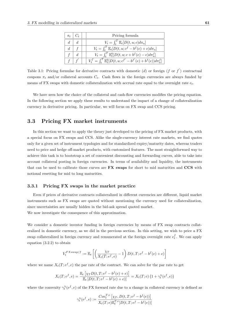
3. FX modelling in collateralized markets 61
πt Ct Pricing formula
d d Vt =∫ TtEt[D(t, u; c)dπu]
d f Vt =∫ TtEt[D(t, u; cf − bf (e) + e)dπu]
f d Vt =∫ TtEbt [D(t, u; c+ bf (e)− e)dπfu]
f f′
V ft =∫ TtEbt [D(t, u; cf
′ − bf ′(e) + bf (e))dπfu]
Table 3.1: Pricing formulae for derivative contracts with domestic (d) or foreign (f or f′) contractual
coupons πt and/or collateral accounts Ct. Cash flows in the foreign currencies are always funded by
means of FX swaps with domestic collateralization with accrual rate equal to the overnight rate et.
We have seen how the choice of the collateral and cash-flow currencies modifies the pricing equation.
In the following section we apply these results to understand the impact of a change of collateralization
currency in derivative pricing. In particular, we will focus on FX swap and CCS pricing.
3.3 Pricing FX market instruments
In this section we want to apply the theory just developed to the pricing of FX market products, with
a special focus on FX swaps and CCS. Alike the single-currency interest rate markets, we find quotes
only for a given set of instrument typologies and for standardized expiry/maturity dates, whereas traders
need to price and hedge off-market products, with customized features. The most straightforward way to
achieve this task is to bootstrap a set of convenient discounting and forwarding curves, able to take into
account collateral posting in foreign currencies. In terms of availability and liquidity, the instruments
that can be used to calibrate those curves are FX swaps for short to mid maturities and CCS with
notional resetting for mid to long maturities.
3.3.1 Pricing FX swaps in the market practice
Even if prices of derivative contracts collateralized in different currencies are different, liquid market
instruments such as FX swaps are quoted without mentioning the currency used for collateralization,
since uncertainties are usually hidden in the bid-ask spread quoted market.
We now investigate the consequence of this approximation.
We consider a domestic investor funding in foreign currencies by means of FX swap contracts collat-
eralized in domestic currency, as we did in the previous section. In this setting, we wish to price a FX
swap collateralized in foreign currency and remunerated at the foreign overnight rate eft . We can apply
equation (3.2.2) to obtain
VFXswap/ft := Et
[(χT
Xt(T ; ef , e)− 1
)D(t, T ; ef − bf (e) + e)
]where we name Xt(T ; ef , e) the par rate of the contract. We can solve for the par rate to get
Xt(T ; ef , e) =Et[χTD(t, T ; ef − bf (e) + e)
]Et [D(t, T ; ef − bf (e) + e)]
= Xt(T ; e)(1 + γχt (ef , e)
)where the convexity γχt (ef , e) of the FX forward rate due to a change in collateral currency is defined as
γχt (ef , e) :=CovT ;e
t
[χT , D(t, T ; ef − bf (e))
]Xt(T ; e)ET ;e
t [D(t, T ; ef − bf (e))]

3.3 Pricing FX market instruments 3. FX modelling in collateralized markets
We can observe that, if the above covariance is null, e.g. this occurs when the spread between the basis
rate bf (e) and the foreign overnight rate ef is a deterministic function of time, then the convexity is zero,
and, in turn, the par rate is equal to the forward rate given in equation (3.1.2). In general, we cannot
estimate the convexity γχt (ef , e) from market data, since V FXswapt and VFXswap/ft share the same quote
on the FX market, and there are not other liquid quotes with this information.
The approach of quoting FX par swap rates regardless of the chosen collateral currency also impacts
FX swap triangulations. Let us consider three currencies x, y, z and the FX swaps between such
currencies. Market practice is to quote par swap rates such that
Xx→zt (T )
Xy→zt (T )
≈ Xx→yt (T ).
By means of the theoretical framework we developed, we want to delimit the validity of such a relationship.
Let us focus on the FX forward rates from currencies x, and y, to currency z. We first assume that the
collateral accounts are in currency z, and remunerated at the overnight rate ezt . We name such rates
Xx→zt (T ; ez) and Xy→z
t (T ; ez). If we calculate the ratio between them, we get
Xx→zt (T ; ez)
Xy→zt (T ; ez)
=Et[χx→zT D(t, T ; ez)]
Et[χy→zT D(t, T ; ez)]= χx→yt
P xt (T ; ez)
P yt (T ; ez)
where the last step comes from the triangulation rules of spot FX market, namely
χx→zt = χx→yt χy→zt
On the other hand, by equation (3.2.3) the FX forward rate from currency x to currency y with
collateralization in currency z at ezt overnight rate is given by
Xx→yt (T ; ez) =
Ebyt [χx→yT D(t, u; by(ez))]
Ebyt [D(t, u; by(ez))]=
Et[χx→zT D(t, u; ez)]
χy→zt Ebyt [D(t, u; by(ez))]= χx→yt
P xt (T ; ez)
P yt (T ; ez)
in which the second equality comes from the equation (3.1.5): Ebt [D(t, T ; bf (e))] = 1χtEt[χTD(t, T ; e)].
Thus, the triangulation rule for FX forward rates holds only if all the rates share the same collateralization
currency
Xx→zt (T ; ez) = Xx→y
t (T ; ez)Xy→zt (T ; ez) (3.3.1)
The same relationship does not hold if we change the collateralization currency. For instance, we consider
the FX forward rates from currency x to currency y with collateralization in currency y at eyt overnight
rate. We get from equation (3.2.4)
Xx→yt (T ; ey) =
Ebyt [χx→yT D(t, u; ey)]
Ebyt [D(t, u; ey)]=
Et[χx→zT D(t, u; ey − by(ez) + ez)]
Et[χy→zT D(t, u; ey − by(ez) + ez)]
=Xx→zt (T ; ez)
(1 + γχ
x→z
t (ey, ez))
Xy→zt (T ; ez)
(1 + γχ
y→z
t (ey, ez))
= Xx→yt (T ; ez)
(1 + γχ
x→z
t (ey, ez)
1 + γχy→z
t (ey, ez)
)
If the market approximation
γχt (ey, ez) ≈ 0 (3.3.2)
is assumed, we obtain that the triangulation rule for FX forward rates is holding again.

3. FX modelling in collateralized markets 63
3.3.2 Cross-Currency swaps
FX swaps are quoted with sufficient liquidity only for short maturities, i.e. up to two-four years
depending on the considered currency pair. For longer maturities, market participant exchange amounts
of currency by means of Cross-Currency swaps (CCS). A CCS is a foreign exchange derivative between two
institutions to exchange the principal and/or interest payments of a loan in one currency for equivalent
amounts, in net present value terms, in another currency. A currency swap should be distinguished from
interest rate swap, for in currency swap, both principal and interest of loan is exchanged from one party
to another party for mutual benefits.
Figure 3.1: A cash flow description of a constant-notional CCS
In the simplest case, depicted in Figure 3.1, each of the two parties lends to the other an amount
of money at the swap start date T0, receives for it (floating) rate interests at dates T1, ..., Ti, ..., TN ,
and gets the notional back at maturity TN . These CCS are called constant-notional because the
principal amount used to value interests is established once for all at inception. For most currency pairs,
standardized CCS are structured such that, at inception, notionals are equivalent (using FX rate for T0)
and the deal is entered at-par.
Figure 3.2: A cash flow description of a marked-to-market CCS
The FX market mainly quotes marked-to-market (MtM) CCS, which are built by appending a series
of at-par single period CCS one after the other. The resulting contract is shown in Figure 3.2, and it
behaves like a pair of rolling loans, where notionals are exchanged at each interest rate payment date,
hence reducing the counterparty risk and the FX risk of the structure. Legs with a MtM notional are

3.3 Pricing FX market instruments 3. FX modelling in collateralized markets
dubbed renotioning or resetting legs, to distinguish them from constant-notional ones.
Most of quoted and liquid CCS have the following features:
• the major currency has a renotioning leg, while a minor currency has a constant-notional leg;
• the major currency has interests indexed to flat Libor rates, while a minor currency has interests
based on Libor rates plus a spread;
• the spread over a minor currency floaters is chosen such that the CCS is at-par (equilibrium spreads
are CCS market quotes);
• payments occur quarterly.
Now we want to value CCS net present value (NPV) and, in order to do that, we take the point of
view of a domestic investor pricing FX swaps, constant-notional CCS and marked-to-market CCS with
collateral posted in domestic currency and remunerated at the same rate e; therefore all foreign flows will
be priced by the formula in the third row of Table 3.1. The extension to different funding strategies is
straightforward by means of the results of Section (3.2).
1. Constant-Notional CCS
Let’s consider a constant-notional CCS, where interests are indexed to domestic and foreign Libor rates
Lxt (T ), t being the fixing date, T the maturity and x ∈ d, f. We assume that the domestic market
quotes single-currency interest rate swaps with a floating leg indexed to the same Libor rates the CCS
domestic leg is indexed to and where the standard collateralization is based on the same collateral rate
e. Hence, we define the domestic Libor forward rate Ft(Ti; e) as the forward for the Libor rate LTi−1(Ti)
when the collateral is posted in natural currency, i.e.
Ft(Ti; e) :=Et[D(t, Ti; e)LTi−1
(Ti)]
Pt(Ti; e)= ETi;et [LTi−1
(Ti)]. (3.3.3)
For sake of generality we allow CCS interests to be equal to Libor rates plus a spread, which we name s
for the domestic leg and sf for the foreign leg. According to first and third rows of Table 3.1, we compute
the CCS price, expressed in domestic units, as
V CCSt := VCCS/dt − V CCS/ft (3.3.4)
where the net present values of the domestic and foreign legs are given by
VCCS/dt := N
(−Pt(T0; e) +
N∑i=1
τi(Ft(Ti; e) + s)Pt(Ti; e) + Pt(TN ; e)
)(3.3.5)
VCCS/ft := χtN
f
(−P ft (T0; e) +
N∑i=1
τi(Fft (Ti; e) + sf )P ft (Ti; e) + P ft (TN ; e)
)(3.3.6)
and where N and Nf stand respectively for the notionals of the domestic and foreign legs, τi is the
year fraction calculated between Ti−1 and Ti. Most importantly, in valuing the net present value of
the foreign leg we introduced the foreign basis forward Libor rates F ft (Ti; e) observed under domestic
collateralization as
F ft (Ti; e) :=Ebt[D(t, Ti; b
f (e))LfTi−1(Ti)
]P ft (Ti; e)
= ETi;bt
[LTi;bTi−1
(Ti)]
(3.3.7)
3. FX modelling in collateralized markets 65
2. Marked-to-market contributions
In this case the resetting of the notional creates an asymmetry between the two legs, so that different
pricing formulae will be needed according to the leg on which the marking-to-market operates.
If the renotioning leg is the domestic one, we get
V CCSt := VMtMCCS/dt − V CCS/ft (3.3.8)
where the net present value of the MtM leg is given by
VMtMCCS/dt = Nf
N∑i=1
Pt(Ti; e)ETi;et
[χTi−1(1 + τi(LTi−1(Ti) + s))
]−Nf
N∑i=1
Pt(Ti; e)ETi−1;et [χTi−1 ]
(3.3.9)
while the constant-notional leg is defined as in Equation (3.3.6).
In the other case, where the foreign leg has a renotioning feature, we have
V CCSt := VCCS/dt − VMtMCCS/f
t (3.3.10)
where the net present value of the MtM leg reads
VMtMCCS/ft = χtN
N∑i=1
P ft (Ti; e)ETi;bt
[1
χTi−1
(1 + τi(L
fTi−1
(Ti) + sf ))]
−χtNN∑i=1
P ft (Ti−1; e)ETi−1;bt [
1
χTi−1
]
(3.3.11)
while the constant-notional leg is defined as in Equation (3.3.5).
These two pricing formulae share the same structure. The contribution of the first summation repre-
sents the redemption of the lending which occurrs at the end of each period plus the payment of matured
interests, while the second summation corresponds to the lending of an amount of currency at each coupon
period start date, such as to be at par with the constant-notional of the other leg. Let us now separately
analyze the structure of the MtM contributions.
Domestic Marked-to-Market Leg
We start by analyzing the domestic MtM leg. The second summation term in equation (3.3.9), where the
exchange rate read at Ti−1 is immediately paid, corresponds to the flow of a FX swap, and it is simply
given byN∑i=1
Pt(Ti−1; e)ETi−1;et [χTi−1 ] = χt
N∑i=1
P ft (Ti−1; e).
On the other hand the first summation, over interests and notional repayments, involves two terms linked
to the correlation structure of discounting, forwarding and exchange rates. In particular we need to
evaluate a FX forward with delayed payment, namely
ETi;et [χTi−1] = ETi;et [XTi−1
(Ti−1; e)] (3.3.12)
and a floating domestic payment with stochastic notional
ETi;et [χTi−1LTi−1
(Ti)] = ETi;et [XTi−1(Ti−1; e)FTi−1
(Ti; e)] (3.3.13)
3.3 Pricing FX market instruments 3. FX modelling in collateralized markets
We wrote these contributions in terms of the forward exchange rate Xt(Ti−1; e) and of the forward Libor
rate Ft(Ti; e), which are martingales under the terminal measures QTi−1;e and QTi;e, respectively. These
two measures are linked by standard Radon-Nikodym derivative
Zt(Ti−1, Ti; e) :=dQTi;e
QTi−1;e
∣∣∣∣t
=Pt(Ti; e)
Pt(Ti−1; e)
P0(Ti−1; e)
P0(Ti; e)(3.3.14)
As a consequence, the first term must be valued taking into account the correlation between the forward
exchange rate and the collateral curve (pure change of measure effect), while the second also need to
incorporate the correlation with forward Libors (change of measure plus covariation). Any estimate of
these contributions requires defining joint distribution with covariation effects. We notice that the FX
delayed payment terms would be present even in the case of a fixed rate MtM CCS.
Foreign Marked-to-Market Leg
We focus on the foreign MtM leg, whose tractation is totally analogous to the one carried on for the
domestic case. The term bound to the lending of a marked-to-market foreign notional is trivial, because
it states that we are lending one unit of domestic currency at each date T0, ..., TN−1 and we get, by means
of Eq. (3.1.5),
χt
N∑i=1
P ft (Ti−1; e)ETi−1;bt
[1
χTi−1
]=
N∑i=1
Pt(Ti−1; e)
Analogously to the domestic MtM case we then write the terms related to the payment of interests
and notional redemptions relying on forward exchange rates and forward Libor rates. We have a FX
forward with delayed payment
ETi;bt
[1
χTi−1
]= ETi;bt
[1
XTi−1(Ti−1; e)
](3.3.15)
and a floating foreign payment with stochastic notional
ETi;bt
[LfTi−1
(Ti)
χTi−1
]= ETi;bt
[F fTi−1
(Ti; e)
XTi−1(Ti−1)
](3.3.16)
In this case the exchange rate to be used for notional purposes is the reverse rate 1χt
converting
domestic units into foreign one. Both expectations involve the basis forward measure QTi;b, under which
the basis forward Libor rate F ft (Ti; e) is a martingale. The forward exchange rate Xt(Ti−1; e), as seen,
is a martingale under the terminal measure QTi−1;e, which is connected to QTi;b by means of the Radon-
Nikodym derivative
Zft (Ti−1, Ti; e) :=dQTi;b
dQTi−1;e
∣∣∣∣t
=Xt(Ti−1; e)P ft (Ti; e)
P ft (Ti−1; e)
P0(Ti−1; e)
X0(Ti−1; e)P f0 (Ti; e)(3.3.17)
Once again, the first expectation involves a change of measure contribution, and depends on the cor-
relation between Xt(Ti−1; e) and Zi−1,it (e; b), while the second also depends on the interplay with basis
forward Libor rates.
At the end of this section we tie together all the analysis brought on so far and quickly sketch a hy-
pothetical bootstrapping procedure to infer basis discount factors, basis forward Libor rates, as well as
correlation terms. We assume here that the market quotes, for a set of maturities, FX swaps, constant-
notional CCS, and MtM CCS both with fixed and floating rate interests.

3. FX modelling in collateralized markets 67
1st step: we can apply Equation (3.1.7)
P ft (T ; e) =Xt(T ; e)
χtPt(T ; e)
to a set of domestic-foreign FX swap with increasing maturities T1, T2,..., TN , such as to derive the
basis discount factors P ft (Ti; e). These basis zero-coupon bonds constitute the fundamental pillars
of a basis discounting curve used to discount foreign flows collateralized in domestic currency.
2nd step: we consider constant-notional CCS and apply formulae of Section (3.3.2) (Point 1) to deduce basis
forward Libor rates F ft (Ti; e) for a set of maturities Ti hence building a basis forwarding curve.
Marked-to-market CCS with domestic renotioning leg and fixed interests let us infer forward FX
rates with deferred payments (Eq. (3.3.12)), which incorporate the correlation between domestic
discounts and FX forwards, while CCS with domestic renotioning leg and floating interests are used
to deduce the terms involving correlations between FX forwards and domestic Libor forwards (Eq.
(3.3.13)). Analogously, Marked-to-market CCS with foreign renotioning leg and fixed interests let
us value inverse forward FX rates with deferred payments (Eq. (3.3.16)), which incorporate the
correlation between basis discounts and FX forwards, while CCS with foreign renotioning leg and
floating interests are helpful to estimate correlations between FX forwards and foreign basis Libor
forwards (Eq. (3.3.13)).

3.4 Effective discounting curve approach 3. FX modelling in collateralized markets
3.4 Effective discounting curve approach
The procedure described above constitute only a theoretical case study; in this section we discuss a
practical curve bootstrapping procedure by approximating the pricing formula of MtM CCS.
We have already said before that the only FX quotes which are actively traded are FX swaps with short
to mid maturities together with MtM CCS with flat floating interests and renotioning for the major
currency leg versus floating interests plus spread and constant notional on the minor currency leg. The
absence of a set of quotes allowing a sequential bootstrap of the foreign basis discounting curve, of the
foreign basis forwarding curve and of correlations driving MtM corrections, forces market players need to
find some approximations. A very common approach to take into account the information embedded in
market quotes, and to quickly price CCS, consists in avoiding direct modelling of the dependencies among
all the components of the swap price formula, and valuing net present values by means of an effective
discounting curve approach.
The most natural way for an investor to achieve this result is to give relevance to its own domestic
currency and price the CCS by means of four curves:
1. a domestic discounting curve, which is the same curve linked to the domestic collateral rate;
2. a domestic forwarding curve, which is the same curve obtained from single-currency standard floaters
quoted in the domestic money market;
3. a foreign currency forwarding curve, which is the same curve obtained from single-currency standard
floaters quoted in the foreign currency money market;
4. an implied foreign currency discounting curve, bootstrapped such as market CCS are repriced at
par.
By means of this procedure we choose to use unadjusted foreign forwards, as if they were paid and
collateralized in their own currency, and incorporate all the corrections discussed above into an implied
foreign currency discounting curve. In this way we deduce an implied foreign currency curve that does
not correspond to the basis foreign currency curve given in equation (1.7.8), and used in the previous
section to present the theoretical curve bootstrapping procedure, unless some approximations hold.
3.4.1 Bootstrapping curves in the FX market
The short end of the implied curve could be straightforwardly stripped by FX swaps by means of Eq.
(3.1.7). Thus, if we call Tc the longest maturity for which we can find on the market liquid quotes of FX
swaps, we can write
P f,implt (T ; e) :=Xt(T ; e)
χtPt(T ; e), T ≤ Tc
where Xt(T ; e) is given by the market.
Then, in order to cover the mid-long part of FX curves (T > Tc), we need to develop simplified pricing
formulae for CCS to be used for bootstrapping purposes. The effective curve approach consists in dis-
regarding all of the contributions that would require a dynamical model and in re-writing in a simple
way the net present values given by equations (3.3.6), (3.3.9), (3.3.11) in terms of implied basis foreign
zero-coupon bonds P f,implt (T ; e). These latters will be calibrated such as to ensure that a set of relevant
market instruments is priced at-par. Equation (3.3.5), wich only involves domestic flows and domestic
collateral, is unchanged. Let us begin by analyzing the MtM domestic leg of a CCS. Its NPV can be cast
3. FX modelling in collateralized markets 69
in the form
VMtMCCS/dt =
N∑i=1
N impli−1 (−Pt(Ti−1; e) + Pt(Ti; e)(1 + τi(Ft(Ti; e) + s))) (3.4.1)
by introducing the coupon-dependent notionals
N implt := NfXimpl
t (Ti; e)
based on the implied forward exchange rates
Ximplt (Ti; e) :=
χtPf,implt (Ti; e)
Pt(Ti; e)
As for the foreign leg, in presence of constant notional (Eq. (3.3.6)), we set
VCCS/ft = χtN
f
(−P f,implt (T0; e) +
N∑i=1
τi(Fft (Ti; e
f ) + sf )P f,implt (Ti; e) + P f,implt (TN ; e)
)(3.4.2)
while if the leg is marked-to-market (Eq. (3.3.11)), we write
VMtMCCS/ft = χt
N∑i=1
Nf,impli−1
(−P f,implt (Ti−1; e) + P f,implt (Ti; e)
(1 + τi(F
ft (Ti; e
f ) + sf )))
where we defined the maturity-dependent notionals
Nf,impli := N
1
Ximplt (Ti; e)
and, in the formulae related to foreign leg, we replaced basis foreign forward Libor rates with the foreign
forward Libor rates F ft (Ti; ef ) which are the rates bootstrapped by a foreign investor by means of its
own money market quotes with the analogous of Equation (3.3.3) discussed before. We use these rates
because we are able to bootstrap them from market quotes.
The rationale behind this definition of implied curve is removing from the equation all the terms
depending on dynamical parameters which cannot be bootstrapped by independent market quotes. In
the following sections we highlight the terms we have approximated to understand the hypothesis under
which the implied curve P f,implt (T ; e) can be identified with the basis curve P ft (T ; e).
Approximating a MtM Domestic Leg
We consider Eq. (3.3.9) and, neglecting correlations between FX spot rate and interest rate risk factors,
get
ETit [χTi−1 ] ≈ Xt(Ti−1; e), ETit [χTi−1LTi−1(Ti)] ≈ Xt(Ti−1; e)Ft(Ti; e).
The assumption
Ximplt (Ti; e) ≈ Xt(Ti; e) (3.4.3)
leads to Eq. (3.4.1) and to the identification P ft (Ti; e) ≈ P f,implt (Ti; e).
Approximating a Constant-Notional Foreign Leg
Let us focus on Eq. (3.3.6). Since the foreign basis forward Libor rates F ft (Ti; e) in such equation cannot
be deduced from independent market quotes, a possible solution is to replace the forward Libor rate by
means of the foreign forward Libor rates as given by the single-currency foreign money market, namely
F ft (Ti; e) ≈ F ft (Ti; ef ). (3.4.4)
3.4 Effective discounting curve approach 3. FX modelling in collateralized markets
This choice naturally suggests to identify P ft (Ti; e) ≈ P f,implt (Ti; e) and to price this leg by means of Eq.
(3.4.2).
Approximating a MtM Foreign Leg Finally, we consider Eq. (3.3.9), disregard correlations between
FX spot rate and interest rate risk factors to approximate
ETi;bt
[1
χTi−1
]≈ 1
Xt(Ti−1; e), ETi;bt
[LTi−1
(Ti)
χTi−1
]≈ F ft (Ti; e)
Xt(Ti−1; e)
and get a simple formula for the net present value of the foreign leg of a MTM CCS as
VMtMCCS/ft ≈ χt
N∑i=1
Nfi−1
(−P ft (Ti−1; e) + P ft (Ti; e)
(1 + τi(F
ft (Ti; e) + sf )
)).
Under the approximations of Eqs. (3.4.3) and (3.4.4) once again we can inteerprete the implied discounts
P f,implt (Ti; e) as proxy for the true basis discount P ft (Ti; e).

Appendix A
Theoretical framework
A.1 Ito calculus: some hints.
Definition A.1. We denote by L2loc the family of processes (ut)t∈[0,T ] that are progressively measurable
with respect to the filtration (Ft)t∈[0,T ] and such that∫ T
0
u2tdt <∞ a.s (A.1.1)
It is interesting to note that the space L2loc is invariant with respect to changes of equivalent probability
measures (see def. (A.5)): if (A.1.1) holds and Q ≈ P then we have of course∫ T
0
u2tdt <∞ Q− a.s.
Definition A.2. An Ito process is a stochastic process X of the form
Xt = X0 +
∫ t
0
usds+
∫ t
0
σsdWs, t ∈ [0, T ] (A.1.2)
where X0 is a F0-measurable random variable, µ ∈ L1loc and σ ∈ L2
loc
Formula (A.1.2) is usually written in the “differential form”
dXt = µtdt+ σtdWt (A.1.3)
Corollary A.1. If X is the Ito process in (A.1.2), then its quadratic variation process is given by
〈X〉t =
∫ t
0
σ2sds
or, in differential terms,
d 〈X〉t = σ2t dt
The differential representation of an Ito process is unique, that is the drift and diffusion coefficients
are determined uniquely1
Theorem A.1. Ito formula for Brownian motion
Let f ∈ C2(R) and let W be a real Brownian motion. Then f(W ) is an Ito process and we have
df(Wt) = f′(Wt)dWt +
1
2f′′(Wt)dt
2
1A proof can be found in [I] p. 1692A complete proof can be found in [I] pp. 170-172
71

A.1 Ito calculus: some hints. A. Theoretical framework
Theorem A.2. Ito formula-general version
Let X be the Ito process in (A.1.3) and f = f(t, x) ∈ C1,2(R2). Then the stochastic process
Yt = f(t,Xt)
is an Ito process and we have
df(t,Xt) = ∂tf(t,Xt)dt+ ∂xf(t,Xt)dXt +1
2∂xxf(t,Xt)d 〈X〉t . (A.1.4)
Remark A.1. Since, by Corollary (A.1), we have
d 〈X〉t = σ2t dt
formula (A.1.4) can be written more explicitly as follows
df =
(∂tf + µt∂xf +
1
2σ2t ∂xxf
)dt+ σt∂xfdWt, (A.1.5)
where f = f(t,Xt).
Definition A.3. An N -dimensional Ito process is a stochastic process of the form
Xt = X0 +
∫ t
0
µsds+
∫ t
0
σsdWs, t ∈ [0, T ] (A.1.6)
where X0 is F0-measurable, W is a d-dimensional Brownian motion, µ ∈ L1loc is a (N × 1)-vector and
σ ∈ L2loc is a (N × d)-matrix.
Formula (A.1.6) can be written in the equivalent differential form
dXt = µtdt+ σtdWt
or, more explicitly
dXit = µitdt+
d∑j=1
σijt dWjt , i = 1, ..., N
Lemma A.1.1. Consider an Ito process X of the form (A.1.6) and set
C = σσ∗.
Then we have ⟨Xi, Xj
⟩t
=
∫ t
0
Cijs ds, t ≥ 0
or, in differential notation,
d 〈X〉t = Ctdt
In practice, given two Ito processes X, Y in RN , the computation of 〈X,Y 〉t can be handled by
applying the following “rule”:
d⟨Xi, Y j
⟩t
= dXitdY
jt
where the product on the right-hand side of the previous equality can be computed using the following
formal rules:
dtdt = dtdW i = dW idt = 0, dW idW j = δijdt,
and δij denotes Kronecker’s delta

A. Theoretical framework 73
δij=
0, i 6= j
1, i = j
Theorem A.3. Let X be an Ito process of the form (A.1.6) and f = f(t, x) ∈ C1,2(R× RN ). Then
df = ∂tfdt+∇f · dXt +1
2
N∑i,j=1
∂xixjfd⟨Xi, Xj
⟩t, (A.1.7)
with f = f(t,Xt) and ∇f = (∂x1f, ..., ∂xN f).
In compact form, if we put C = σσ∗ and recall Lemma (A.1.1), then the formula (A.1.7) becomes
df =
1
2
N∑i,j=1
Cijt ∂xixjf + µt · ∇f + ∂tf
dt+∇f · σtdWt
=
1
2
N∑i,j=1
Cijt ∂xixjf +
N∑i=1
µit∂xif + ∂tf
dt+
N∑i=1
d∑h=1
∂xifσiht dW
ht .
A.2 Bank account and risk neutral measure
In order to understand the modern interest rate market after the credit crunch, we must set up a
framework with solid theoretical basis able to explain the observed data, or, in other words, to price plain
vanilla derivatives according to the available market quotations.
The (spot) instantaneous rate, abbreviated into short rate, is an abstract rate spanning an infinitesi-
mal time interval (with infinitesimal rate tenor). In fact, setting T1 = t, T2 = T and taking the limit
t+ ← T we obtain
Rk(t, T ) −−−−→t+←T
R1(t, T ) −−−−→t+←T
R∞(t, T ) −−−−→t+←T
Lk(t, T ) −−−−→t+←T
r(t)
From any equation above, we may obtain, setting T = t+ dt,
N(t+ dt) = N(t)[1 + r(t)dt]
where N(t) is the nominal al time t and dt is an infinitesimal time interval. Thus the dynamics of N(t)
is given by
dN(t) := N(t+ dt)−N(t) = N(t)r(t)dt
and can be easily integrated over a finite time interval [T1, T2] to obtain
N(T2) = N(T1)exp
∫ T2
T1
r(t)dt.
Thus, the short rate is a continuously compounded annual rate.
The bank account, or money market account, is, in financial mathematics, an ideal financial instrument
representing the behaviour of an abstract loan that rewards its holder with the risk free rate. Denoting
with B(t) the bank account value at time t, it must evolve in time according to the dynamicsdB(t) = r(t)B(t)dt,
B(0) = 1.
A.3 Feynman-Kac theorem A. Theoretical framework
This simple differential problem can be integrated to obtain the solution
B(T ) = B(0)exp
∫ T
0
r(t)dt
The factor B(0) = 1 on the right hand side (r.h.s) is tipically omitted, in this case one should remember
that the dimensionality is correct (currency on both sides).
Being the short rate a stochastic process, also the bank account is a stochastic process. From a fi-
nancial point of view, the bank account is such that one unit of currency invested at time t = 0 accrues,
over an infinitesimal time interval dt, at the (stochastic) short rate r(t).
Thus the bank account is particularly suitable as reference asset, or numeraire, since it allows to put into
relation amounts of currencies observed at different times.
The value (price) of any contract Π can be expressed in units of B(t) and B(T ) through the risk neutral
pricing formulaΠ(t)
B(t)= EQ
t
[Π(T )
B(T )
]Π(t) = EQ
t [D(t, T )Π(T )]
D(t, T ) :=B(t)
B(T )= exp
[−∫ T
t
r(u)du
]
where Q denotes the risk neutral measure associated to the numeraire B(t) and EQt [.] denotes the expec-
tation at time t < T under measure Q .
We remark that the stochastic discount factor is adimensional, being the ratio between two bank account
values, and it depends on the short rate over the time interval [t, T ].
In case of a contract paying multiple coupons Π(T1), ...,Π(TN ) at multiple cash flow dates T1, ..., TNwe have
Π(t) =
N∑i=1
EQt [D(t, T )Π(T )]
Notice that the expectation is a linear operator. The expression above can be written in integral form
Π(t) =
∫ T
t
EQt [D(t, u)dπ(u)]
where T = TN , by introducing the cumulative coupon process
π(t) :=
N∑i=1
1t>TiΠ(Ti).
In fact
Π(t) =
∫ T
t
EQt [D(t, u)dπ(u)] =
∫ T
t
EQt [D(t, u)
N∑i=1
δ(Ti − u)Π(u)du] =
N∑i=1
EQt [D(t, T )Π(T )]
A.3 Feynman-Kac theorem
The Feynman-Kac theorem, under certain assumptions, allows us to express the solution of a given
partial differential equation (PDE) as the expected value of a function of a suitable diffusion process
whose drift and diffusion coefficient are defined in terms of the PDE coefficients.

A. Theoretical framework 75
Theorem A.4 (Feynman-Kac). Let A be a generic asset with price process A(t) solution of the SDE
dA(t) = µ(t, A)dt+ σ(t, A)dWQ(t), 0 ≤ t ≤ T,
µ, σ ∈ L2[0, T ],
A(t = 0) = A0 ∈ R+,
under some probability measure Q . Let also Π be a derivative on A with price Π(t, A(t)) = Π(t) at time
t, solution of the parabolic PDE
LΠ(t) = r(t)Π(t),
L :=∂
∂t+ µ(t, A)
∂
∂A+
1
2σ2(t, A)
∂2
∂2A
Π ∈ C1,2[[0, T ]× R], σ(t, A)Π(t) ∈ L2[0, T ],
Π(T ) ∈ R+, t ∈ [0, T ] ⊂ R+
Then the derivatives’ price Π(t) admits the representation
Π(t) = EQt [D(t, T )Π(T )],
D(t, T ) = exp
[−∫ T
t
r(u)du
]
where Q is the measure such that
dA(t) = µ(t, A)dt+ σ(t, A)dWQ(t)
Theorem A.5 (Generalised Feynman-Kac). In case of the more general parabolic PDE
Lµ = r(t, A(t))Π(t) + Φ(t, A(t)),
we have the more general expectation
Π(t) = EQt
[D(t, T,A)Π(T ) +
∫ T
t
D(t, u,A(u))φ(u,A(u))du
],
D(t, T,A) = exp
[−∫ T
t
r(u,A(u))du
]
where Q is the measure such that
dA(t) = µ(t, A)dt+ σ(t, A)dWQ(t)3
This theorem is important because it establishes a link between the PDE’s of traditional analysis and
physics and diffusion processes in stochastic calculus. Solutions of PDE’s can be interpreted as expecta-
tions of suitable transformations of solutions of stochastic differential equations and vice versa.
3See e.g Darrel Duffie (2001), Tomas Bjork (2009)
A.4 Zero Coupon Bond A. Theoretical framework
A.4 Zero Coupon Bond
The Zero Coupon Bond is the simplest interest rate derivative. It is a contract in which one party
guarantees to the other party the payment of one unit of currency at maturity date T , with no other
payments. The contract payoff at time T is thus denoted by P (T ;T ) = 1 and the contract value at time
t < T by P (t;T ). The dimension is currency (c) and the units are, e.g., Euro. Using the risk neutral
pricing formula we have the pricing expression
P (t;T ) = EQt [D(t, T )P (T ;T )] = EQ
t [D(t, T )].
As for the bank account the dimensionality of the equation above is correct when one remembers that
there is an hidden nominal amount N = 1 units of currency on the r.h.s.
Notice that the Zero Coupon Bond value, being the price of a contract between two counterparties,
has to be exactly known at any time t < T , and thus it is a deterministic (not stochastic) quantity (being
an expectation). This is the main difference with respect to the stochastic discount factor.
Both the stochastic discount factor D(t, T ) and the Zero Coupon Bond P (t;T ) “move” an amount of
money backward in time. In financial terms we say that the amount of money is discounted from time
T to time t < T , thus D(t, T ) and P (t;T ) are both called discount factors. The reciprocals 1D(t;T ) and
1P (t;T ) ”move” an amount of money forward in time from t to T > t and are called capitalization factors.
The main difference between the two types of discount/capitalization factors is that, in general, the
Zero Coupon Bond is deterministic, while the stochastic discount factor is not. Thus, given a deterministic
amount of money N(T2) at time T2, we have
N(T1) = P (T1;T2)N(T2),
N ′(T1) = D(T1;T2)N(T2) 6= N(T1),
EQT1
[N ′(T1)] = P (T1;T2)N(T2) = N(T1)
where N(T1) is deterministic and N ′(T1) is, in general, stochastic.
In case of deterministic interest rates, we have D(t, T ) = P (t;T ) and N ′(T1) = N(T1) are all determin-
istic quantities.
There exist a relationship between interest rates and Zero Coupon Bonds. Using the general expres-
sion
N(T1) = P (T1;T2)N(T2)
and the definitions of simple/discrete/continuous compounded rates give before, we obtain the following
expressions
Interest rate Expression in terms of Zero Coupon Bond
Simple compounding (Libor) L(T1, T2) = 1τ(T1,T2)
[1
P (T1;T2) − 1]
Discrete compounding Rk(T1, T2) = k
P (T1;T2)1
kτ(T1,T2)− k
Continuous compounding R∞(T1, T2) = − 1τ(T1,T2) lnP (T1;T2)
We may invert the preceding relations to express the Zero Coupon Bond in terms of the different
interest rates

A. Theoretical framework 77
Interest rate Expression in terms of Zero Coupon Bond
Simple compounding (Libor) P (T1, T2) = 11+L(T1;T2)τ(T1,T2)
Discrete compounding P (T1, T2) = 1[1+
Rk(T1,T2)
k
]kτ(T1,T2)
Continuous compounding P (T1, T2) = e−R∞(T1,T2)τ(T1,T2)
The Zero Coupon Bond is particularly important in interest rate modeling because, similarly to the
bank account, it can be used as reference asset (numeraire) to put into relation amounts of currencies
observed at different times.
The value (price) of any asset π at any times t and T > t can be expressed in units of P (t, T ) and
P (T, T ), respectively, through the T -forward (Libor) pricing formula
Π(t)
P (t;T )= EQT
t
[Π(T )
P (T ;T )
]= EQT
t [Π(T )]
Π(t) = P (t;T )EQTt [Π(T )]
where Q T denotes the T -forward (Libor) measure associated to the numeraire P (t;T ).
A.5 Change of measure
Radon-Nikodym theorem
Definition A.4. Given any two measures P, Q on (Ω,F), we say that Q is P-absolutely continuous on
F if, for every A ∈ F such that P(A) = 0, we have Q(A) = 0. In this case we write Q P or Q F Pif we want to highlight the σ-algebra that we are considering; indeed it is apparent that the notion of
absolute continuity depends on the σ-algebra under consideration: if G ⊆ F are σ-algebras, then QG Pdoes not necessarily imply that QF P.
Definition A.5. If Q P and P Q, then we say that the measure P and Q are equivalent and we
write P ≈ Q. In case P, Q are probability measures, Q F P implies that the P-negligible events in Fare also Q-negligible, but the converse may not be true. Obviously, if Q F P, then for every A ∈ Fsuch that P (A) = 1 we have Q = 1, i.e. the certain events for P are certain also for Q, but the converse
is not generally true.
Theorem A.6. Let (Ω,F ,P) be a finite-measure space. If Q is a finite measure on (Ω,F) and QF P,
then there exists L : Ω→ R, L ≥ 0, such that
i) L is F-measurable;
ii) L is P-integrable;
iii) Q(A) =∫ALdP for every A ∈ F
Further, L is P-almost surely unique (i.e. if L′ verifies the same properties of L, then P(L = L′) = 1).
We say that L is the density of Q with respect to P on F or also the Radon-Nikodym derivative of Qwith respect to P on F and we write without distinction L = dQ
dP or dQ = LdP. In order to emphasize the
dependence on F , we also write
L =dQdP
∣∣∣∣F
(A.5.1)

A.5 Change of measure A. Theoretical framework
Remark A.2. Let P, Q be the probability measures on the space (Ω,F) with Q P and set L = dQdP .
Using Dynkin’s theorem, we can show that X ∈ L1(Ω,Q) if and only if XL ∈ L1(Ω,P) and in that case
EQ[X] = EP[XL] (A.5.2)
where EP and EQ denote the expectations under the probability measures P and Q respectively. In other
words ∫Ω
XdQ =
∫Ω
X
(dQdP
)dP
and this justifies the notation (A.5.1).
On the probability space (Ω,F ,P) we consider a sub-σ-algebra G of F and a probability measure
QF P (therefore also QG P). We denote by LF (resp. LG) the Radon-Nikodym derivative of Q with
respect to P on F (resp. on G). In general LF 6= LG since LF may not be G-measurable. On the other
hand, we have
LG = EP[LF |G]
Indeed LG is integrable and G-measurable and we have∫G
LGdP = Q(G) =
∫G
LGdP , G ∈ G
since G ∈ F .
A result on the change of probability measure for conditional expectations, analogous to formula (A.5.2),
is given by the following:
Theorem A.7 (Bayes’ formula). Let P, P be the probability measures on (Ω,F) with QF P. If X ∈ L1
(Ω,Q), G is a sub-σ-algebra of F and we set L = dQdP
∣∣∣∣F
, then we have
EQ[X|G] =EP[XL|G]
EP[L|G]
Proof. We put V = EQ[X|G] and W = EP[L|G]. We have to prove that
i) Q(W > 0) = 1;
ii) VW = EP[XL|G]
Concerning i), since W = 0 ∈ G, we have
Q(W = 0) =
∫W=0
LdP =
∫W=0
WdP = 0.
Concerning ii), VW is obviously G-measurable and for every G ∈ G we have∫G
VWdP =
∫G
EP[V L|G]dP =
∫G
V LdP
=
∫G
EQ[X|G]dQ =
∫G
XdQ =
∫G
XLdP
Definition A.6. Q N1 , Q N2 are equivalent martingale measures associated to the two numeraires N1
and N2 ifΠ(t)
N1(t)= EQN1
t
[Π(T )
N1(T )
]Π(t)
N2(t)= EQN2
t
[Π(T )
N2(T )
]

A. Theoretical framework 79
Comparing the two equations above we obtain
Π(t) = EQN1
t
[N1(t)
N1(T )Π(T )
]= EQN2
t
[N2(t)
N2(T )Π(T )
]thus the change from measure Q N1 to measure Q N2 is given by
EQN2
t
[Π(T )
N2(T )
]=N1(t)
N2(t)EQN1
t
[Π(T )
N1(T )
]Why changing the numeraire?
Let X(t) the stochastic process underlying the payoff of the derivative Π:
• Suppose that N2(t) is a numeraire, a strictly positive tradable asset and X(t)N2(t) is the price of
a tradable asset;
• In this case [X(t)N2(t)]N2(t) is a martingale under Q 2, such that we may assume simple stochastic
dynamics for it with simple distributions under Q 2, e.g. lognormal martingale dynamics
dX(t)
X(t)= σ(t)dWQN2
(t)
lnX(T ) ≈ N
[lnX(t)− 1
2
∫ T
t
σ2(u)du;
∫ T
t
σ2(u)du
]
Now, if Π(t)N2(t) is simple enough w.r.t. Π(t)
N1(t) , we are able to compute its expectation under Q 2.
EQN2
t
[Π(T )
N2(T )
]Example A.1 (Change between risk neutral and T−forward measures). If we choose
QN1 = Q,QN2 = QT
N1(t) = B(t), N2(t) = P (t;T )
we obtain
Π(t) = EQt [D(t, T )Π(T )] = B(t)EQ
t
[Π(T )
B(T )
]= B(t)
P (t;T )
B(t)EQTt
[Π(T )
P (T ;T )
]= P (t;T )EQT
t [Π(T )]
Example A.2 (Change between T1 and T2 forward measures). If we choose
QN1 = QT1 ,QN2 = QT2 T1 < T2
N1(t) = P (t;T1), N2(t) = P (t;T2)
we obtain
Π(t) = EQT1t
[P (t;T1)
P (T ′;T1)Π(T ′)
]= EQT2
t
[P (t;T2)
P (T ′;T2)Π(T ′)
]t ≤ T1 ≤ T2 ≤ T ′

A.5 Change of measure A. Theoretical framework
Example A.3 (Change between foreign and domestic risk neutral measures). If we choose
QN1 = Qf ,QN2 = Qd
N1(t) = Bf (t), N2(t) = Bd(t)
Πd(t) = xfd(t)Πf (t)
where xfd is the spot exchange rate from currency f to currency d, we obtain
Πf (t) = EQft [Df (t, T )Πf (T )]
Πd(t) = EQdt [Dd(t, T )Πd(T )]
= xfd(t)EQft [Df (t, T )Πf (T )]
= EQdt [Dd(t, T )xfd(T )Πf (T )]
hence
EQft [Df (t, T )Πf (T )] = EQd
t
[Dd(t, T )
xfd(T )
xfd(t)Πf (T )
], ∀t ≤ T
Example A.4 (Change between risk neutral and forward swap measures). If we choose
QN1 = Q,QN2 = QS
N1(t) = B(t), N2(t) = A(t,S)
where A(t, S) =∑ni=1 P (t, Si)τk(Si−1, Si), we obtain
Π(t) = EQt [D(t, T )Π(T )] = EQ
t
[B(t)
B(T )Π(T )
]= A(t,S)EQS
t
[Π(T )
A(T, S)
], ∀t ≤ T ≤ S0
.
The Girsanov theorem shows how a SDE changes due to changes in the underlying probability measure.
It is based on the fact that the SDE drift depends on the particular probability measure P in our
probability space (Ω,F , (Ft)t,P), and that, if we change the probability measure in a “regular” way, the
drift of the equation changes while the diffusion coefficient remains the same. The Girsanov theorem can
be thus useful when we want to modify the drift coefficient of a SDE. Indeed, suppose that we are given two
measures P∗ and P on the space (Ω,F , (Ft)t). Two such measures are said to be equivalent, written P∗ ∼P, if they share the same sets of null probability (or of probability one, which is equivalent). Therefore
two measures are equivalent when they agree on which events of F hold almost surely. Accordingly, a
proposition holds almost surely under P if and only if it holds almost surely under P∗. Similar definitions
apply also for the measures restriction to Ft, thus expressing equivalence of the two measures up to time
t. When two measures are equivalent, it is possible to express the first in terms of the second through
the Radon-Nikodym derivative. Indeed, there exists a martingale ρt on (Ω,F , (Ft)t,P) such that
P∗(A) =
∫A
ρt(w)dP(w), A ∈ Ft
A. Theoretical framework 81
which can be written in a more concise form as
dP∗
dP
∣∣∣∣Ft
= ρt
The process ρt is called the Radon-Nikodym derivative of P∗ with respect to P restricted to Ft. When
in need of computing the expected value of an integrable random variable X, it may be useful to switch
from one measure to another equivalent one. Indeed, it is possible to prove that the following equivalence
holds:
E∗[X] =
∫Ω
X(w)dP∗(w) =
∫Ω
X(w)dP∗
dP(w)dP(w) = E
[XdP∗
dP
]where E∗ and E denote expected values with respect to the probability measures P∗ and P, respectively.
More generally, when dealing with conditional expectations, we can prove that
E∗[X|Ft] =E[X dP∗
dP |Ft]
ρt
Theorem A.8. Change of numeraire (Girsanov)
Given two numeraires N1(t), N2(t), and a generic asset X(t) following the stochastic diffusion processes
under the martingale measure Q 1 associated to N1,
dX(t) = µQ1
X [t,X(t)] + σX [t,X(t)]′ · dWQ1(t)
dN1(t) = µQ1
N1[t,N1(t)] + σN1
[t,N1(t)]′ · dWQ1(t)
dN2(t) = µQ1
N2[t,N2(t)] + σN2
[t,N2(t)]′ · dWQ1(t)
dWQ1
i (t)dWQ1
j (t) = ρij(t)dt, i, j = 1, ..., F
where W (t) is a F-dimensional vector of correlated brownian motions under Q 1 and the volatilities are
F-dimensional vectors, with 1 ≤ F ≤ 3. The dynamics of X(t) under Q2 is
dX(t) = µQ2
X [t,X(t)] + σX [t,X(t)] · dWQ2(t)
µQ2
X [t,X(t)] = µQ1
X [t,X(t)] + σX [t,X(t)] · ρ(t) ·[σN2 [t,X(t)
N2(t)− σN1
[t,X(t)]
N1(t)
]′dWQ2(t) = dWQ1(t)− ρ(t) ·
[σN2
[t,X(t)
N2(t)− σN1
[t,X(t)]
N1(t)
]′dt
A.6 Replication
• Market:
we assume a market M trading n assets A with price, cumulative dividend and cumulative gain
processes
G(t) = A(t) +D(t) =
G1(t)
...
Gn(t)
=
A1(t)
...
An(t)
+
D1(t)
...
Dn(t)
• Asset price dynamics:
we assume Ito process under real measure P
dA(t) = µ(t,A)dt+ σ(t,A) · dW P (t), A(0) = A0
dWPi (t)dWP
j (t) = ρijdt, ∀i, j = 1, ..., d

A.6 Replication A. Theoretical framework
• Cumulative dividend dynamics:
we assume continuous dividends proportional to asset A with instantaneous dividend rate rD(t)
dD(t) = A(t)rD(t)dt, D(0) = 0
D(t) =
∫ t
0
A(u)rD(u)du
• Cumulative gain dynamics:
dG(t) = dA(t) + dD(t) = [µ(t,A) + rD(t)A(t)]dt+ σ(t,A) · dW P (t)
G(0) = A(0) +D(0) = G0
• Derivative price dynamics:
the market trades also a derivative, with price at time t denoted by Π(t), depending on the other
assets A. The dynamics of the derivative price is obtained from Ito’s lemma
dΠ(t) =∂Π
∂tdt+
∂Π′
∂A· dA(t) +
1
2dA(t)′ · ∂
2Π
∂2A· dA(t)
= Lµ(t,A)Π(t)dt+∂Π′
∂A· σ(t, bsA) · dW P (t)
L :=∂
∂t+ µ(t,A)′ · ∂
∂A+
1
2
n∑i,j=1
d∑f=1
σi,f (t,A)σi,j(t,A)∂2
∂Ai∂Aj
• Exchange rate:
since we want to deal with the multiple currency funding case, we introduce in M also a spot
exchange rate at time t: Nα(t) = xα,β(t)Nβ(t)
• Trading strategy:
a trading strategy is a (multidimensional) process Θ(t) such that
V (t,Θ,A) := Θ(t) ·A(t), V (0,Θ,A) = Θ(0)′ ·A(0) := V0(Θ,A)
G(t,Θ,A) :=
∫ t
0
Θ(u)′ · dG(u), G(0,Θ,A) = 0
D(t,Θ,A) := G(t,Θ)− [V (t,Θ,A)− V0(Θ,A)], D(0,Θ,A) = 0
are the price, cumulative gain and cumulative dividend processes, respectively. The components Θ
of the trading strategy are interpreted as the number of units (or nominal) of the asset A held at
time t.
• Self financing:
a trading strategy Θ is self-financing if its associated dividend process is null
D(t,Θ,A) = 0
⇒ dG(t,Θ,A) = dV (t,Θ,A)
Intuitively, a self-financing strategy is such that it’s cumulated gains are generated only by the
changes in the asset prices, and no additional cash flows occur during it’s life.

A. Theoretical framework 83
• Replication:
a derivative price Π(t) is replicated through a self-financing trading strategy Θ(t) if
Π(t,A) = V (t,Θ,A), ∀t ∈ [0, T ]
GΠ(t,A) = G(t,Θ,A), ∀t ∈ [0, T ]
where GΠ(t, A) is the cumulative gain process associated to derivative Π.


Bibliography
[I] Pascucci A., PDE and Martingale Methods in Option Pricing, Springer, Bocconi University Press,
Milan, 2011
[II] Brigo D. and Mercurio F., Interest Rate Models-Theory and Practice With Smile, Inflation and
Credit, Springer-Verlag, Berlin, 2006
[III] Moreni N. and Pallavicini A., FX Modelling in Collateralized Markets: foreign measures, basis curves
and pricing formulae, http://papers.ssrn.com/sol3/results.cfm, 2015
[IV] Lesniewski A., Interest Rate and Credit Models, http://www.math.nyu.edu/ alberts/spring07/, 2007
85