BIS CCA-009-2011

May 2011

FX co-movements: disentangling the role of global market factors, carry-trades and idiosyncratic components

Paper prepared for the 2nd BIS CCA Conference on

“Monetary policy, financial stability and the business cycle”

Ottawa, 12–13 May 2011

Authors*: José Gonzalo Rangel

Affiliation: Bank of Mexico

Email: jgrangel@banxico.org.mx

* This paper reflects the views of the author and not necessarily those of the BIS or of central banks

participating in the meeting.

1

FX Comovements: Disentangling the Role of Market Factors, Carry-Trades and Idiosyncratic Components*

Jose Gonzalo Rangel† Bank of Mexico

Preliminary Draft (March 10, 2011)

Abstract

This paper models high and low frequency dynamic components of FX excess return correlations and examines their relationship with economic fundamentals. A factor currency pricing model is used to characterize the correlation structure of FX excess returns. I provide evidence on high levels of comovement in FX markets during the post-crisis (or recovery) period following the 2008 financial turmoil. I find that while the low frequency component of systematic volatility shows an increasing trend during this recent period, the low frequency component of idiosyncratic volatilities presents declining patterns. These two effects explain the increase in average long-term correlations. In terms of idiosyncratic effects, my results suggest that country-specific inflation levels and real output growth significantly affect the time-series and cross-sectional variation of long-term FX idiosyncratic volatilities.

Keywords: Comovements, FX markets, global factors, idiosyncratic volatilities, economic fundamentals.

JEL classification: F31, G12, G15.

* The views expressed in this paper are those of the author and do not necessarily reflect those of Banco de Mexico. The author is grateful to Gustavo Abarca for his excellent research assistance and to seminar participants at the 2nd Annual CIRPÉE Applied Financial Time Series Workshop in Montreal for helpful discussion and comments. † Author Contact: Av. 5 de Mayo No. 2 Col. Centro, México D.F., C.P. 06059, México. Tel: (5255) 5237-2708. Email: jgrangel@banxico.org.mx.

2

1. Introduction

The variation over time of FX comovements plays a key role in the assessment and

management of currency risk. For example, its analysis helps to evaluate the global

exposure of a currency portfolio, hedge investment positions, diversify the portfolio,

and price currency derivatives. In this regard, the term structure of such comovements

can provide a broader view to distinguish between short and long-term risk exposure in

FX markets. Despite the practical importance of this distinction, no empirical studies

have analyzed jointly the dynamic features of term FX comovements and their

economic determinants.

This paper fills this gap and examines the term dynamic behavior of the comovement of

FX excess returns and its relation with economic fundamentals, including global

components of the stochastic discount factor and country-specific (idiosyncratic)

macroeconomic variables. FX excess returns are measured from the point of view of a

US investor that manages a portfolio of foreign currencies.1 The data show that, in

addition to correlation clustering and short-term dynamics driven by the arrival of high

frequency return information, there is striking evidence of long-term variation (trends)

in the return correlation structure. This makes unappealing the application of dynamic

correlation models that mean-revert to constant levels. Instead, I apply the recent

approach of Rangel and Engle (2009) that captures high and low frequency fluctuations

of asset comovements and relaxes the restriction of mean reversion to a constant

unconditional correlation matrix. Under this framework, the high frequency correlation

mean-reverts to a slow-moving low frequency correlation component. The model of

Rangel and Engle (2009) assumes a factor asset pricing structure to characterize asset

returns. In the present case, I consider the factor specification of Lustig, Roussanov, and

Verdelhan (2009). This framework assumes that the stochastic discount factor is linear

in the pricing factors.2 They suggest a currency pricing model with two factors: 1) a

carry-trade risk factor based on a zero-cost strategy that goes long in a portfolio of

1 FX excess returns are defined as the return on buying a foreign currency in the forward market and then selling it in the spot market after one month. 2 This asset pricing approach incorporates, as a particular case, the seminal model of Backus, Foresi, and Telmer (2001). The main critical difference is that this earlier model does not allow the loadings of the common component to differ across currencies.

3

currencies of high interest rates countries and short in a portfolio of low interest rates

countries, and 2) an FX market factor that measures the average excess return of all

foreign currency portfolios.3 In addition, I incorporate the effect of a third factor

associated with equity market risk. The resulting three factor model is used to

characterize the systematic component of FX excess returns and isolate their

idiosyncratic risk.

This decomposition not only facilitates the interpretation of changes in the correlation

structure, but also allows to link economic fundamentals with the different components

of currency risk. In particular, the factor structure implies a correlation specification that

depends on systematic and idiosyncratic variances, factor loadings (betas), and

covariances across both systematic and idiosyncratic terms. Under this framework,

while the level of comovement between two assets (or markets) increases as the

systematic volatility -or the level of the factor loadings (betas)- raises, it also declines as

the idiosyncratic volatility of one (or both) assets increases.

The Factor-Spline-GARCH model of Rangel and Engle (2009) produces a slow moving

correlation component that depends on the low frequency systematic and idiosyncratic

volatilities. Also, the model includes a high frequency correlation component that is

driven by high frequency components of these volatilities and by conditional covariance

terms that capture temporal variation in the betas and the effects of latent omitted

factors. The two term correlation components appear to be consistent with the empirical

patterns observed in the studied dataset, which includes 29 currencies during the period

1999-2010.4 These currencies are measured with respect to the U.S. dollar and

correspond to floating exchange regimes. The data frequency is weekly in order to avoid

asynchronous trading biases.5 The starting date was selected to match the introduction

of the Euro as a common currency in the European zone. An exploratory analysis based

3 The carry-trade factor has been examined in recent studies, which suggest that this factor conveys a premium that has become more important in recent years (see Brunnermeier, Nagel, and Pedersen (2009), Lustig and Verdelhan (2007) and Lustig, Roussanov, and Verdelhan (2009)). Menkhoff, Sarno, Schmeling, and Schrimpf (2009) use the second factor to analyze global FX volatility. 4 The pricing factors are constructed from an extended sample that includes 52 countries. It incorporates the cases analyzed in Menkhoff, Sarno, Schmeling and Schrimpf (2009), and four additional countries: Chile, Colombia, Peru, and Turkey. 5 The approach used in this paper can be modified to incorporate higher frequency data. For example, Engle and Rangel (2009) synchronize daily returns and estimate the Factor-Spline-GARCH model to characterize correlations dynamics in international equity markets.

4

on model-free rolling correlations motivates the importance of introducing different

types of dynamics into these components to explain the variation in the comovement of

currency returns over time.

The present paper documents historical high levels of comovements in FX markets

during the most recent years. Although it is natural to expect high levels of asset

comovements during global crisis periods (see, for example, Ang and Bekaert (2002)),

the levels of correlations in FX markets have remained high for about two years. My

evidence suggests that this behavior is explained by increasing patterns in the long-term

volatility components of the risk factors, as well as by declining idiosyncratic

volatilities since the peak reached at the end of 2008.6

To complement the analysis of the correlation components, I perform time series and

cross-sectional analyses based on linear projections of low frequency FX idiosyncratic

volatilities on country-specific fundamental macroeconomic variables, such as real

growth, inflation, money supply growth, the volatilities of these variables, as well as the

volatility of short-term interest rates.7 I follow the approach of Engle and Rangel (2008)

by using seemingly unrelated regressions (SUR) and dynamic panel models. My results

suggest that long-term FX idiosyncratic volatilities are significantly affected by

inflation and growth. In particular, low growth and high inflation are associated with

higher levels of FX idiosyncratic volatilities. Also, higher volatility of inflation is

positively related to FX idiosyncratic volatility. These results are statistically significant

and robust to controlling for transaction costs in FX markets. Nevertheless, the

explanatory power of these macroeconomic variables appears to be modest. In addition,

my evidence indicates that long-term FX idiosyncratic volatility may be influenced by a

common time varying component that shows high correlation with stock market

volatility.

Comovements in FX markets have been empirically explored in Kroner and Sultan

(1993), Tong (1996), Sheedy (1998), Gagnon, Lypny and McCurdy (1998), and Chang

6 Other causes may be temporal or permanent increases in the factor loadings. Although the Factor-Spline-GARCH framework can capture temporal variation in the betas, it has limitations because the betas are assumed to be stationary and mean-reverting to their unconditional versions. So, the model only captures temporal deviations of the factor loadings from such constant unconditional terms. 7 Engel and West (2005) use similar measures of fundamentals and relate them to various theoretical exchange rate models.

5

and Kim (2001). Their results suggest time variation and clustering in currency

correlations. However, these studies focus on stationary frameworks and none of them

capture long-term trends in FX correlations along with high frequency changes. The

present study not only provides further evidence of significant time variation and

clustering in FX excess returns comovements, but also discusses trend behavior in the

recent years. Moreover, it links such a pattern to the evolution of global risk

components, countries’ sensitivities to each of them, and country-specific

macroeconomic factors. The present paper also contributes to explain patterns in FX

comovements during the most recent post-crisis period.

The paper has the following structure. Section 2 provides a summary of the correlation

structure implicit in factor asset pricing models. It also presents the factor specification

estimated for FX markets and a summary of the Factor-Spline-GARCH econometric

approach. Section 3 describes the data to compute FX excess returns and the proxies for

the global risk factors. It also illustrates stylized facts in the recent comovement of FX

excess returns using model-free measures. Section 4 presents the model estimation

results and examines the dynamic behavior of the correlation determinants. In Section 5,

I perform time series and cross-section regression analyses of FX idiosyncratic

volatilities. Section 6 provides concluding remarks.

2. Factor Asset Pricing Models and Correlation Structure

2.1 Standard factor models and correlations

To explain the recent evolution of the comovement (correlation) across currency

markets, I use standard factor asset pricing models. The typical example of such models

is the popular APT (Arbitrage Pricing Theory) model of Ross (1976). Under this

framework, the return of an asset (ri,t) can be written as a linear combination of K

systematic risk factors (f1,t, f2,t,…, fK,t) that capture the common variation in individual

asset returns, and an idiosyncratic return (εi,t) that is uncorrelated with respect to the

factors.

, ,1 1, ,2 2, , , ,...i t i i t i t i K K t i tr f f f (1)

6

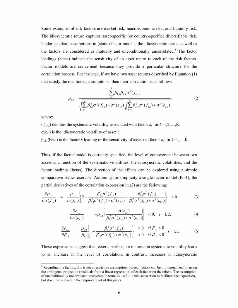
Some examples of risk factors are market risk, macroeconomic risk, and liquidity risk.

The idiosyncratic return captures asset-specific (or country-specific) diversifiable risk.

Under standard assumptions in (static) factor models, the idiosyncratic terms as well as

the factors are considered as mutually and unconditionally uncorrelated.8 The factor

loadings (betas) indicate the sensitivity of an asset return to each of the risk factors.

Factor models are convenient because they provide a particular structure for the

correlation process. For instance, if we have two asset returns described by Equation (1)

that satisfy the mentioned assumptions, then their correlation is as follows:

21, 2, ,

11,2

2 2 2 2 2 21, , 1, 2, , 2,

1 1

( ),

( ) ( ) ( ) ( )

K

k k k tk

K K

k k t t k k t tk k

f

f f

(2)

where:

σ(fk,t) denotes the systematic volatility associated with factor k, for k=1,2,…,K.

σ(εi,t) is the idiosyncratic volatility of asset i.

βi,k (beta) is the factor k loading or the sensitivity of asset i to factor k, for k=1,…,K.

Thus, if the factor model is correctly specified, the level of comovement between two

assets is a function of the systematic volatilities, the idiosyncratic volatilities, and the

factor loadings (betas). The direction of the effects can be explored using a simple

comparative statics exercise. Assuming for simplicity a single factor model (K=1), the

partial derivatives of the correlation expression in (2) are the following:

2 2 2 21,2 1,2 2,1 1, 1,1 1,

2 2 2 2 2 21, 1, 2,1 1, 2, 1,1 1, 1,

( ) ( )2 0

( ) ( ) ( ) ( ) ( ) ( )t t

t t t t t t

f f

f f f f

(3)

1,2 ,1,2 2 2 2

, , 1, ,

( )0, 1, 2,

( ) ( ) ( )i t

i t i i t i t

if

(4)

2 2

,11,2 1,2 ,1 1,

2 2 2,1,1 ,1 ,1 1, ,

00( )1 , 1,2.

00( ) ( )ii t

ii i i t i t

sifi

sif

(5)

These expressions suggest that, ceteris paribus, an increase in systematic volatility leads

to an increase in the level of correlation. In contrast, increases in idiosyncratic

8 Regarding the factors, this is not a restrictive assumption. Indeed, factors can be orthogonalized by using the orthogonal projection (residuals from a linear regression) of each factor on the others. The assumption of unconditionally uncorrelated idiosyncratic terms is useful in this subsection to facilitate the exposition, but it will be relaxed in the empirical part of this paper.

7

volatilities are associated with declines in the level of correlation. Moreover, if the betas

become larger in absolute value, the level of correlation increases. However, the

empirical examination of these effects requires further considerations about the

underlying assumptions in (1) and (2). Indeed, changes in correlations can be due to

other effects that are not captured in specification (2), for example, omitted factors and

the conditional interactions across both factors and idiosyncratic terms (see Rangel and

Engle (2009)). These effects are incorporated in the specification of the conditional high

frequency correlation component, described later in this section.

2.2 A factor specification for currency excess returns

Currency excess returns can be defined in terms of spot and forward exchange rates. In

particular, the excess return on a currency is the return on buying the foreign currency in

the forward market and then selling it in the spot market one month later. Following the

notation of Lustig et al. (2009) and Menkhoff et al. (2009), the log excess return can be

written as:

1 1,t t trx f s (6)

where f is the log of the forward exchange rate and s denotes the log of the spot

exchange rate.

Lustig et al. (2009) form currency portfolios based on the level of foreign interest rates

and find that two factors explain more than 80% of the return variation on these

portfolios.9 After performing a principal components analysis, they find that the first

principal component is indistinguishable from the average portfolio return. They

interpret this first factor as a level factor. The second principal component is basically

the difference between the return on the last portfolio and that on the first portfolio. This

factor is interpreted as a slope factor and basically captures the excess return on a carry-

trade zero-cost strategy that goes long on the portfolio of the highest interest rate

currencies and short on that of the lowest interest rate currencies.

9 They allocate all the currencies in their sample to six portfolios ranked from low to high interest rates, which are measured at the end of the period. Thus, the portfolios are rebalanced at the end of every month.

8

Their model can be written in terms of a stochastic discount factor that is linear in the

pricing factors. In particular, the Euler pricing equation leads to the following moment

condition:

1 1( ) 0,kt t tE M Rx (7)

where 1ktRx is the excess return on portfolio k and Mt+1 is the stochastic discount factor

that is assumed to be linear in the pricing factors as follows:

1 11 ( ).t tM b F (8)

In this expression Ft+1 is a vector of factors, b is a vector of factor loadings, and μ is a

vector of factor means. Under this setup, expected excess returns can be written in terms

of the vector of prices of risk λ as:

( )k kE Rx

(9)

where k

is a vector of betas (regression coefficients) associated with the linear

projection of portfolio k excess returns on the factors. In the currency context, the

following specification that separates systematic and idiosyncratic components is

consistent with the described framework:10

1 1 1 1( )k k k kt t t t trx E rx F u

(10)

The idiosyncratic component ( 1ktu ) does not bear factor systematic risk. The empirical

implementation of this framework requires a selection of proxies for the factors and

some assumptions about the error term. Following the results of Lustig et al. (2009), I

consider an equally weighted portfolio of currency excess returns (denoted by RX) and

the carry-trade portfolio (HMLFX) suggested by these authors.11 In addition, and

different from the specification of Lustig et al. (2009), I consider a third factor that

incorporates equity global market risk (Rm). This factor can be motivated either

theoretically, by the fact that the stochastic discount factor should be effective to price

equities and other asset classes as well; or empirically, by the highly significant betas

obtained from the estimation of the model (see Table 2 in Section 4).

10 Alternatively, following Backus et al. (2001), the depreciation rate can be seen as the log difference of the local and foreign stochastic discount factors (SDFs). Assuming that each (log) SDF is linear in a subset of the considered risk factors, and given that rx interest rate differential – depreciation rate (see Equation (24)), this type of beta representation for excess returns can be formulated as a reasonable approximation. 11 The RX portfolio is also analyzed in Menkhoff et al. (2009). I use a sample closer to theirs because it is broader than the sample of Lustig et al. (2009).

9

Other important differences of my approach with respect to that of Lustig et al. (2009)

are related to the data frequency and the analyzed dynamic features. In particular, while

these authors focus on the cross-sectional variation of quarterly aggregated currency

returns on a few portfolios, I use higher frequency (weekly) data on excess returns of

individual currencies and focus on the time series variation of higher order moments. In

particular, based on the specification in (10), I characterize the dynamics of second

moments of currency excess returns and relate them to macroeconomic variables.

2.3 An econometric model for FX comovements

In this section, I describe the econometric model applied to characterize different

features of the dynamics of FX comovements. The use of the Factor-Spline-GARCH

framework of Rangel and Engle (2009) is motivated by the factor asset pricing structure

in (10) and the goal of capturing short-term patterns and non-stationary long-term trends

in the second moments of FX returns. Following this approach and assuming

conditional normality, I parameterize the empirical pricing relation in (10) as:

1 , 1 ,| , ~ ( , ), | ~ (0, ),t t t u t t t F tx F N BF H F N Htr (11)

where

, , , , , , , , , , ,u t u t rx rx t u t F t F t f f t F tH R and H R

, , , , ,rx rx t f f tR and R are correlation matrices

, , ~ -u t F tand Diagonal Spline GARCH (12)

Here, 2, ,u t u t tD and 2

, ,F t F t tG , where , ,{ },u t i tdiag 1

2,{ }t i tD diag g , for

i=1,2,…,N, , , ,{ },F t f j tdiag and 1

2, ,{ }t f j tG diag g , for j=1,2,…,K. Based on the

discussion in the previous subsection, Ft=(f1,t=RXt, f2,t=HMLFX,t, f3,t=Rmt)’. As in Engle

and Rangel (2008), the , 'i t s are specified as exponential quadratic splines and the gi,t’s

are unit asymmetric GARCH processes. Element by element, we have:

, , 1 , , , ,

, , , , , , ,

( ) ' , 1,..., ,

, 1,..., ,

i t i t t i t i t i t i t i t

j t f j t f j t f j t

u rx E rx F g i N

f g j K

(13)

where the high and low frequency variance components of the idiosyncratic terms are

defined as:

10

, 1

22, 1 0, 1

, , 1, 1 , 1

2

, 0 11

12

exp ( ) , 1,..., ,

i t

i

i t ri tii t i i i i i i t

i t i t

k

i t i i is ss

u Iug g

c w t w t t for i N

(14)

and the variance components of the three factors are:

, 1

,

22, 1 0, , 1

, , , , , , , , , 1, , 1 , , 1

2

, , , , ,0 , , 11

12

exp ( ) , 1,...,

j t

f j

j t ff j j tf j t f j f j f j f j f j f j t

f j t f j t

k

f j t f j f j f j s ss

f Ifg g

c w t w t t for j K

(15)

The model is completed by adding dynamics to the covariation across factor and

idiosyncratic innovations using the dynamic conditional correlation (DCC) specification

of Engle (2002) for the vector t 1, 2, , ,1, , ,( , ,..., , ,..., ) 't t N t f t f K tε . Hence, its

correlation structure can be expressed as a partitioned correlation matrix:

, , , ,

1 t, , , ,

(ε ) ,rx rx t rx f t

tf rx t f f t

R RV

R R

(16)

where Rrx,rx,t describes the correlations across idiosyncratic innovations, Rrx,f,t

characterizes the correlations across idiosyncratic and factor innovations, and Rf,f,t

describes the correlations across factor innovations. As a result, the whole model

parameterizes the conditional covariance matrix of returns in equation (10) as:

1/2 1/2 1/2 1/2 1/2 1/2

1 t t , , , , , , , , , ,cov ( , ') ,t f t t f f t t f t f rx t t t t t rx f t t t rx rx t t tx x B G R G B BR D D R B D R Dr r (17)

and the following expression defines the low frequency covariance:

1/2 1/21 , ,' ,t f t t rx rx tB B R (18)

where ,rx rxR is the unconditional correlation of idiosyncratic innovations. Analogous

expression for the high and low frequency correlation matrices are:

1/2 1/21 t t 1 t( , ') {cov( , ')} cov ( , ') {cov( , ')} ,t t t t t t tcorr x x diag x x x x diag x xr r r r r r r r (19)

1/2 1/2 1/2 1/2 1/2 1/2 1/2 1/2

, , , , , ,{ ' } ( ' ) { ' }t f t t rx rx t f t t rx rx t f t t rx rx tLFR diag B B R B B R diag B B R (20)

The main property of this model is that the high frequency correlation component in

(19) mean-reverts toward the time-varying low frequency correlation matrix in (20) that

can capture long-term trend behavior in the comovement of FX excess returns.

11

3. Data and stylized facts

The sample used in my empirical analysis includes daily returns that are aggregated up

to a weekly frequency to avoid major concerns of biases from non-synchronous trading

activity. I examine the comovement across the 29 currencies described in Table 1.

Nevertheless, I use an extended sample of currencies to construct the RX and HMLFX

factors. In particular, I consider a sample of 52 countries that includes the 48 currencies

considered in Menkhoff et al. (2009) plus the cases of Chile, Colombia, Peru, and

Turkey. Using an extended sample for the computation of the factor portfolios is useful

for obtaining more precise measures of the common components and avoiding the

concern of simultaneity problems. I use the MSCI World Index as a proxy for the equity

market factor. Daily returns on this index are aggregated up to a weekly frequency. The

series on forward and spot exchange rates were obtained from Bloomberg. The sample

period goes from January 1999 to August 2010. The initial date was selected to match

the introduction of the Euro as a common currency in most of the European region. The

factor portfolios are constructed following Lustig et al. (2009) and Menkhoff et al.

(2009). As in these studies, I also examine the sensitivity of the results to the effect of

transaction costs.

Another goal of this study is to examine the cross-sectional determinants of FX

idiosyncratic volatility that, as shown in Section 4, plays an important role in explaining

FX comovements. For this analysis, I consider various measures of FX fundamentals

following Engel and West (2005). In particular, I use quarterly data on GDP, inflation

(measured through Consumer Price Indices), money supply (defined as M2), and short-

term interest rates for the 29 countries described in Table 1. The International Financial

Statistics (IFS) database from the International Monetary Fund (IMF) is the source of

macroeconomic information.

In order to explore some patterns of international comovement in FX markets, I

construct a time series that measures the average correlation at each point in time. This

average is taken from the individual correlations across the excess returns on the 29

currencies described in Table 1. Specifically, the time t correlation between the

depreciation rates of two currencies is estimated from the sample correlation based on a

12

rolling sample of 52 weeks (1 year). Then, at every week, the cross-sectional average of

all the pairwise correlations is considered. Thus, the average global correlation is

defined as follows:

, ,1

1 1

( 1)

N

t i j ti j iN N

(21)

where ρi,j,t is the correlation between the excess returns on currencies i and j at week t.

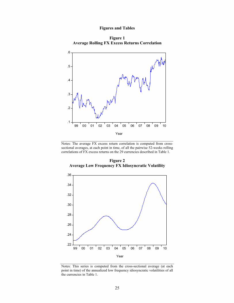
Figure 1 shows the dynamic behavior of the average FX comovement. It illustrates a

pattern consistent with a positive trend.12 Also, an upward jump is observed after the

crisis and its level has remained high since the end of 2008. In fact, in terms of the

(almost) 12 years included in the sample, this level of comovement has reached

historical maximums during the last two years. These patterns suggest that standard

correlation models that mean-revert to constant levels may be restrictive to describe the

features of the data. Thus, considering the presence of either long-term trends or

regimes appears to be important for modeling FX comovements. This motivates the

advantages of using a framework such as the one described in Section 2, which

incorporates long-term trend behavior in the correlation structure of asset returns.

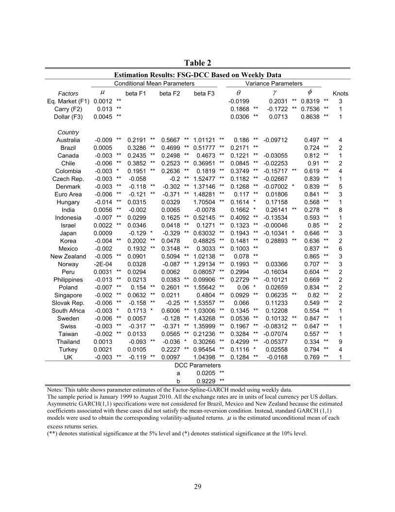
4. Estimation results

The factors and excess returns are constructed following Lustig et al. (2009). Based on

specification (10), I estimate a Factor-Spline-GARCH model using equations (11)-(20)

and the definition of excess returns in (6).13 The results of the estimation are shown in

Table 2. In most cases, there is evidence of highly significant volatility persistence

(volatility clustering). Regarding the unconditional betas, with exception of India, at

least one of the factors showed a significant effect on each currency excess return. The

FX market beta is significant in 28 out of 29 cases, the stock market beta shows

statistical significance in 17 cases, and the carry-trade beta does it in 23 cases. The signs

are also consistent with the economic intuition. For example, the betas of the FX

(equally weighted) market portfolio are in general positive and their average is close to

one. The carry-trade betas are consistent with the findings of Lustig et al. (2009), but in

this case focusing on individual currencies instead of aggregated portfolios. Indeed, the

12 In results not reported in this paper, I find that a regression of this series on a linear trend (over the sample period) suggests a trend coefficient that is positive and statistically significant at the 1% level. 13 The estimation strategy follows the two-step GMM approach described in Rangel and Engle (2009).

13

carry-trade betas tend to be negative and large in magnitude for low interest rate

countries, such as Denmark, the Czech Republic, the Euro Area, Japan, Norway, the

Slovak Republic, Sweden, Switzerland, and Thailand. In contrast, they tend to be

positive and large for higher interest rate countries such as Australia, Brazil, South

Africa, New Zealand, and Mexico. In terms of the stock market beta, it is positive for

most of the cases, but Denmark, the Euro Area, Japan, the Slovak Republic,

Switzerland, Thailand, and the UK.

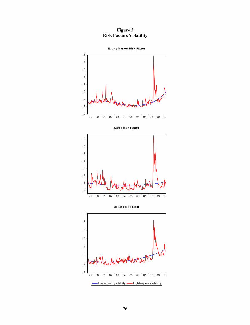
The volatility estimates presented in the last four columns of Table 2 also tend to show

the usual patterns. The average ARCH effect is around 0.18 and the average GARCH

effect is 0.70. However, the leverage effect only showed some statistical significance in

27% of the cases. For this parameter, it is difficult to find a sign pattern. The average

number of knots of the low-frequency volatility splines is 2.7, which indicates the

presence of about three main inflection points in the average long-term trend of FX

idiosyncratic volatilities, within the 12-year sample period examined in this paper.

Figure 2 illustrates the patterns in this low frequency average FX idiosyncratic volatility

during the sample period. The top rows of Table 2 show the estimates for the systematic

factors. Here the ARCH effects are relatively small (even insignificant for the stock

market factor) and the volatility persistence GARCH effects are large. Consistent with

the literature, the leverage effect is highly significant for the stock market factor.14 For

the carry-trade factor the results suggest a puzzling negative and significant sign pattern.

A possible explanation may be that, when the carry-trade strategy yields losses, there is

a decline in the carry-trade activity and therefore in the volatility of the corresponding

excess returns. For the FX market factor, the ARCH and GARCH effects are highly

significant and lie near the expected order of magnitudes; however, the leverage effect

is insignificant. Figure 3 illustrates the patterns in these systematic volatilities.

The bottom rows of Table 2 present the second step DCC estimates. The standard

second step likelihood of Engle (2002) is applied. Hence, only countries that have

complete data available from the beginning to the end of the sample period are included.

This leaves out from the second step estimation the cases of Brazil, Chile, Colombia,

14 See, for example, Black (1976), Christie (1982), Campbell and Hentschel (1992), and Bekaert and Wu (2000).

14

Israel, Korea, Peru, and Slovak Republic.15 The DCC estimates are also as expected and

suggest high persistence in the correlation structure and a significant response to the

cross-product innovations.

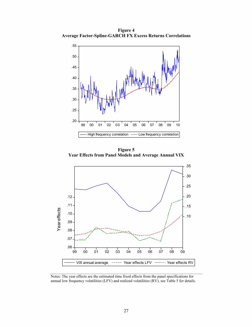
The results are illustrated at an aggregate level in Figure 4. Based on the expressions in

equations (19) and (20), this figure shows the average high and low frequency

correlations. Consistent with the stylized facts presented in Section 3, both components

show increasing patterns during the sample from correlation magnitudes around 0.30-

0.35 to magnitudes close to 0.50. This is an increase of around 50% within this 12-year

period that may capture the shifts from low to higher correlation regimes. Models that

do not account for these effects may show important drawbacks for capturing the long-

term evolution of FX return comovements. In this regard, perhaps the most remarkable

and appealing property of this model with respect to stationary DCC specifications is

that the high frequency component mean-reverts to the low frequency one, which shows

an increasing long-term trend that appears more consistent with the patterns observed in

the data. Moreover, it suggests advantages for forecasting at medium and long horizons.

In fact, this component suggests that FX excess returns correlations will mean-revert to

levels around 0.45 instead of 0.35, which is the average sample correlation.

Nevertheless, it is important to have an economic notion of what variables may affect

the long-term level of correlations. The following section provides some insightful

results.

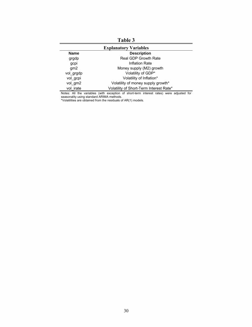
5. Economic determinants of long-term FX idiosyncratic volatilities

5.1 Long-term volatility measures and explanatory variables

The link between economic variables and FX idiosyncratic volatilities is relevant not

only for examining possible economic drivers of the low frequency component of FX

correlations, but also for utilizing this relationship to construct out-of-sample forecasts.

To select the variables that may be related to long-term idiosyncratic volatilities, I

15 However, these countries are considered for the time series and cross-sectional analyses of the determinants of FX idiosyncratic volatility presented in Section 5, where an unbalanced panel of idiosyncratic volatilities is constructed. An alternative approach to incorporate all the cases in the second step DCC estimation may be the Composite Likelihood Method of Engle, Shephard and Sheppard (2009). In results not reported, I find that the estimates obtained from this method are very close to those presented in Table 2.

15

appeal to economic theory and consider an asset market approach to exchange rates (see

Obstfeld and Rogoff (1996) and Engel and West (2005)). In particular, based on the

decomposition of Engel and West (2005), in which they represent the exchange rate as a

present value relationship in terms of observable and unobservable current and expected

future values of fundamentals, the nominal exchange rate can be defined as the log of

the home currency price of foreign currency (US dollar) and expressed as:

0 0

( ) ( ) ,j jt t t j t t j t t

j j

s b E f b E z F U

(22)

where ft denote a measure of observed fundamentals in the home country relative to

abroad (the US), and zt denote not observable economic fundamentals (or measurement

errors). A stationary version of (22) can be written as: 16

t t ts F U (23)

From this relationship, it is natural to relate | |ts to a group of explanatory variables

determined by | |tF and tF . In particular, among the possible observable

fundamentals (Ft), Engel and West (2005) consider the log of home money supply (mt),

the log of the home price level (pt), the level of the home short-term interest rate (it),

and the log of output (yt). Furthermore, they find that a number of theoretical FX models

can fit into the framework given in (22).17 It is possible to associate these fundamentals

to the FX excess return equation given in (6) since this expression can be rewritten as:

*1 1 1.t t t t t t trx f s s i i s (24)

Considering these results, the next step is to define an empirical specification for FX

idiosyncratic volatilities that incorporates the time series and cross-sectional variations

of the series estimated in Section 4 from the Factor-Spline-GARCH model. In this

regard, I follow the approach of Engle and Rangel (2008) and define annual measures of

long-term FX idiosyncratic volatility, for year t and currency i, based on the low

frequency idiosyncratic volatility of each currency and the corresponding realized

measure:

16 The evidence of Engel and West (2005) suggests that st~I(1) and, based on the set of fundamentals

considered in their analysis, (0)~t

f I . Moreover, they do not find evidence of cointegration between st

and ft, thus they conclude that Ut~I(1). 17 For example, the framework can be consistent with monetary models such as Frenkel (1976, 1979), and Mussa (1976), and open economy macroeconomic models such as Obstfeld and Rogoff (2002).

16

152 2

, , ,1

1,

52i t i t dd

Lvol

(25)

152 2

2, , ,

1

,i t i t dd

Rvol u

(26)

where , ,i t d is the weekly low frequency volatility in (14), observed in country i at week

d of year t, and ui,t,d is the estimated idiosyncratic innovation in (10).

5.2 Linear specifications and results

To explain the variation of these proxies, I set the following two systems of linear

equations for annual low frequency and realized volatilities, respectively:

, , ,' , 1, 2,..., , 1,2,..., ,i t i t t i t tLvol x t T i N (27)

, , ,' , 1, 2,..., , 1,2,...,i t i t t i t tRvol x t T i N (28)

where ,i tx is a vector of explanatory variables at the annual frequency. Based on the

discussion in the previous paragraphs of this section, economic variables linked to

fundamentals are included in this vector. In particular, I consider real GDP growth, the

level of inflation, the growth rate of money supply, the volatilities of these three

variables, and the volatility of short-term interest rates.18 These variables are

summarized in Table 3. The volatilities of the mentioned macroeconomic variables are

estimated from quarterly data and the residuals from autoregressive processes of order

one that are used to fit each of the macroeconomic time series. In particular, for each of

these series (y), the absolute values of the residuals from an AR(1) model are obtained,

and the corresponding volatility is measured as their yearly average, as follows:19

1

12,

2

log , ,

1.

4

t t t t t

t

y t jj t

y c u u u e

e

(29)

As argued by Engle and Rangel (2008), it is likely that the high persistence of the

dependent variables will lead to important serial correlation in the error terms of (27)

and (28). To address this issue, I follow their approach and estimate the systems using

two methodologies: the SUR method of Zellner (1962) and a linear fixed-effects panel

18 For each country, the levels of real GDP, inflation, and money supply were adjusted for seasonal effects using standard ARIMA methods. 19 This approach was used in Engle and Rangel (2008).

17

model with serially correlated innovations described by an AR(1) dynamic process. For

the former, the systems incorporate different intercepts to capture time fixed effects. For

the panel specification, time fixed effects and country-specific random effects are

considered. Thus, the error terms in (27) is modeled as follows:

, , ,i t t i i t (30)

where

, , 1 ,

,

,

time fixed effect

~ (0, )

~ (0, )

t

i

i t i t i t

i t

i t i

iid

iid

A similar structure is considered for the error term in (28). Also, it is important to note

that the examined panel is unbalanced and it includes a larger number of countries than

the DCC estimation (see footnote 14).

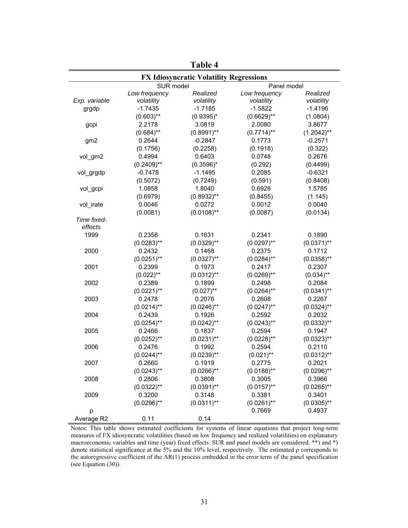
The estimation results are presented in Table 4. The first panel shows the SUR estimates

for each of the long-term idiosyncratic volatility proxies. The second one presents the

linear panel estimates.20 The first column shows the results for low frequency FX

idiosyncratic volatilities. In this case, while the effect of real GDP growth is negative

and significant, those of inflation and volatility of money supply are positive and

significant. The estimated coefficients of other explanatory variables did not show

statistical significance and, with exception of GDP volatility, their signs were positive.

The results for the annual realized FX idiosyncratic volatilities are similar regarding the

significant effects of real GDP growth, inflation and money supply volatility. In this

case, however, the volatilities of inflation and short-term interest rates showed statistical

significance and evidence of positive effects on realized FX idiosyncratic volatilities.

The results from the panel models, with error structure given in (30), indicate again that,

for low frequency idiosyncratic volatilities, the coefficient of GDP growth is negative

and significant, and the one of inflation is positive and significant. Nevertheless,

although with a positive sign, money supply volatility is no longer significant. As in the

SUR case, the other explanatory variables do not show statistical significance.

Regarding the realized idiosyncratic volatility measure, the only variable that is

20 An indicator for emerging markets was also introduced as a control variable in the SUR systems. It was not significant and did not affect other estimation results.

18

statistically significant is the level of inflation and it presents a positive sign, as

expected.

Overall, a comparison of the results from the two estimation approaches indicates that,

for low frequency volatilities, the significant effects of real growth and inflation are

robust to different assumptions about the correlation structure in the error terms of the

linear specifications. For the annual realized measures, the level of inflation appeared as

the only robust significant variable. It is also important to mention that the explanatory

power of these regressions was modest, on average.21 This suggests that the variation in

FX volatilities may largely come from the systematic risk factors, and that the

idiosyncratic component shows only a mild response to country-specific fundamentals.

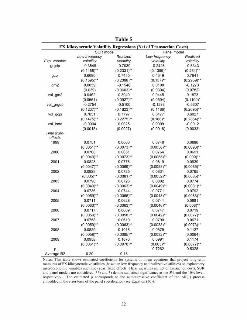
5.3 Robustness: adding transaction costs

Transaction costs play an important role in the construction of excess returns and risk

factors proxies. Hence, it is important to verify their effect on the estimation results. In

this regard, I compute the realized excess return net of transaction costs following

Lustig et al. (2009). They define the net log currency excess return for an investor that

goes long in the foreign currency as:

1 1,l b at t trx f s (31)

where btf is the bid price at which the investor sells dollars forward and 1

ats is the ask

price at which he buys dollars in the spot market. An analogous expression can be

obtained for an investor that goes short in the foreign currency.

I use this definition of net FX excess returns (based on a long position) and compute the

corresponding new time series for each country, as well as the dollar and carry-trade

factors. Then, I re-estimate the FSG-DCC model described in Section 4 and obtain

measures of net FX idiosyncratic volatilities for each of the currencies in Table 1. These

series are used to compute net long-term idiosyncratic volatility proxies based on

equations (25) and (26). Finally, the resulting variables are projected on the

21 The average R2 of the SUR system was 0.l3 for the case of low frequency idiosyncratic volatility and 0.16 for the annual realized volatility. These values are considerable smaller than those obtained in Engle and Rangel (2008) for equity long-term volatilities.

19

macroeconomic variables described in Table 3, using the SUR and dynamic panel

approaches discussed earlier.

Table 5 shows the estimation results for the long-term net FX idiosyncratic volatilities.

For the net low frequency measure, they are qualitatively similar to those presented in

Table 4. As before, the two estimated specifications suggest that, while real GDP

growth has a negative significant effect on low frequency idiosyncratic volatility, the

effect of inflation is positive and significant. The main difference with respect to the

results without transaction costs is that, in this case, the volatility of inflation has a

significant (positive) coefficient in both specifications.

Regarding the annual realized idiosyncratic volatility measure, although the results are

also qualitatively similar to those of the case without transaction costs, in the sense that

all the effects show the same direction, they vary slightly more in terms of statistical

significance. For example, the volatilities of money supply and inflation are now

significant variables with positive signs in both specifications, and the volatility of real

GDP shows a negative significant coefficient. Nonetheless, from tables 4 and 5, it is

clear that the only variable that is significant in all of the examined specifications is

inflation. Then, variables like real GDP growth and volatility of inflation show

statistical significance across models and for the two long-term FX idiosyncratic

volatility measures. Overall, controlling for the effect of transaction costs does not

appear to change the main empirical findings of this paper regarding the significant

effect of inflation and GDP growth on long-term FX idiosyncratic volatilities.

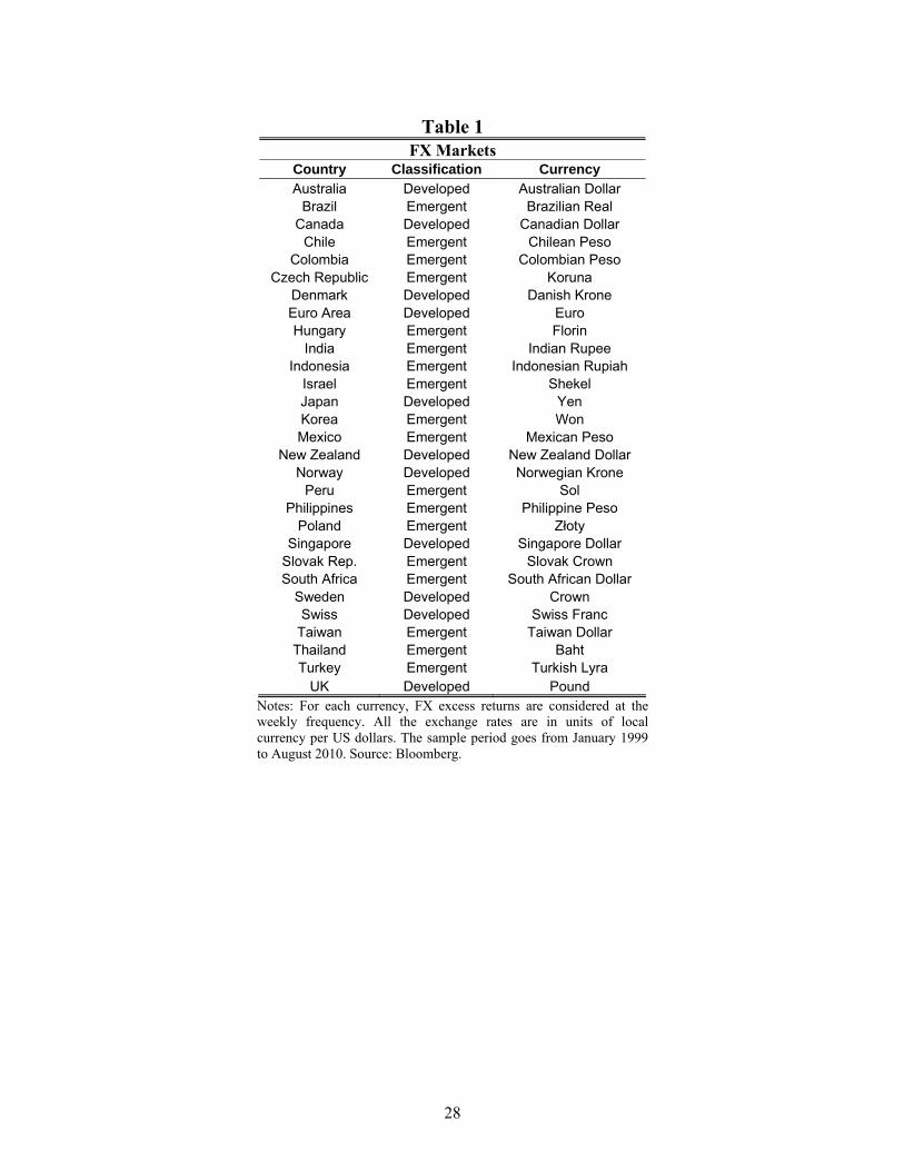
Finally, I examine the patterns of the time fixed effects from the panel specifications

associated with each long-term FX idiosyncratic volatility measure. These time effects

are shown in Figure 5, along with the S&P500 Volatility Index (VIX). As it is visually

suggested from this figure, the fixed effects associated with the two long-term

idiosyncratic volatility measures are highly correlated with the VIX index. Indeed,

while the sample correlation between the low frequency volatility fixed effects and this

index is 0.77, the realized volatility fixed effects and the VIX index show a correlation

of 0.75. These results suggest that there may be an omitted volatility risk factor in the

model that appears as a common component in long-term FX idiosyncratic volatilities.

Moreover, this evidence may be seen as consistent with the results of Menkhoff et al.

20

(2009), which find that an FX market volatility factor (in levels) has important

explanatory power for the cross-section of currency excess returns.

6. Concluding remarks

This paper examines different types of dynamics in the comovements of currency

returns. In particular, it documents that, in addition to the well known clustering and

time variation in conditional correlations at short horizons, there may be long-term

trends in the comovements of FX returns. These trends require alternative dynamic

correlations methods with the ability to capture this type of non-stationarity in the data.

I present a strategy that combines the Factor-Spline-GARCH model of Rangel and

Engle (2009) with the linear factor currency pricing model of Lustig et al. (2009). The

resulting framework allows not only the possibility of capturing the apparent trend

comovement patterns shown by FX excess returns data, but also a further examination

of the economic variables that may drive such a trend behavior.

The specification for FX excess returns considers the dollar and the carry-trade factors

introduced by Lustig et al. (2009). In addition, I incorporate a global equity market

factor to characterize the systematic component of excess returns. The resulting three

factor specification leads to a particular form of the FX correlation structure. The

dynamic correlation model of Rangel and Engle (2009) describes high and low

frequency dynamic patterns in each of the components of this correlation structure,

distinguishing the role of systematic and idiosyncratic terms. The model suggests a non-

monotonic increasing behavior in the comovement of FX excess returns during the

period 1999-2010. The average correlation increased in about 50% from the beginning

to the end of this period, based on a sample of 29 currencies. This effect appears

stronger during the last three years of the sample, which include the years surrounding

the financial crisis of 2008. These findings are consistent with the patterns observed

from model free measures. The model captures these effects by the combination of an

increasing systematic volatility and mixed idiosyncratic volatility effects that, on

average, appear to be declining since early 2009.

While it is reasonable to think that equity and FX market volatilities have remained high

due to low prospects of global growth and high macroeconomic uncertainty, less is

21

known about the economic determinants of FX idiosyncratic volatility. This paper

addresses this question and performs a time series and cross-sectional analysis of the

economic determinants of long-term FX idiosyncratic volatilities. The explanatory

variables were selected following the economic theory about FX fundamentals. From

different model specifications and long-term volatility measures, my results suggest that

the most robust variables that explain the variation in such volatilities are inflation and

real GDP growth. In particular, the evidence of this paper indicates that the higher the

level of inflation (and its volatility), the higher the level of FX idiosyncratic volatility;

also, the lower the level of real output growth, the higher as well the level of FX

idiosyncratic volatility. Moreover, my results indicate that long-term FX idiosyncratic

volatilities may be affected by a common factor associated with market volatility risk.

These findings are important, not only because they are helpful to understand part of the

dynamic behavior of global FX comovements, but also because they may provide

important insights for forecasting volatilities and correlations at long horizons. In

addition, my results point out that there is still an important part of the FX idiosyncratic

volatility variation that is not explained by the considered fundamentals. Hence, further

research is needed in this regard to improve our understanding of the dynamics in FX

excess returns comovements and volatilities.

References

Ang, A., and G. Bekaert (2002), “International Asset Allocation with Regime Shifts,”

Review of Financial Studies, 15, 1137-1187.

Backus, D., S. Foresi, and C. Telmer (2001), “Affine Models of Currency Pricing:

Implications for the Forward Premium Anomaly,” Journal of Finance, 56, 281–311.

Bekaert, G., and G. Wu (2000), “Asymmetric Volatility and Risk in Equity Markets,”

Review of Financial Studies, 13, 1-42.

Black, F. (1976), “Studies of Stock Price Volatility Changes,” Proceedings of the 1976

meetings of the American Statistical Association, Business and Economics Statistics

Section, American Statistical Association:177-181.

22

Brunnermeier, M., S. Nagel, and L. Pedersen (2009), “Carry trades and currency

crashes,” NBER Macroeconomics Annual, 23, 313–347.

Campbell, J., and L. Hentschel (1992), “No News is Good News: An Asymmetric

Model of Changing Volatility in Stock Returns,” Journal of Financial Economics, 31,

281–318.

Chang, Kook-Hyun and Myung-Jig Kim, (2001), “Jumps and time-varying correlations

in daily foreign exchange rates,” Journal of International Money and Finance, 20, 611-

637.

Christie, A. (1982), “The Stochastic Behavior of Common Stock Variances: Value,

Leverage and Interest Rate Effects,” Journal of Financial Economics, 10, 407-432.

Engel, C., and K. West (2005), “Exchange Rates and Fundamentals,” Journal of

Political Economy 113, 485–517.

Engle, R. (2002), “Dynamic conditional correlation: a simple class of multivariate

generalized autoregressive conditional heteroskedasticity model” Journal of Business

and Economic Statistics 20, 339-350.

Engle, R., and J.G. Rangel (2008), “The Spline-GARCH Model for Low Frequency

Volatility and its Global Macroeconomic Causes,” Review of Financial Studies, 21,

1187-1222.

Engle, R.F., and J.G. Rangel (2009), “High and Low Frequency Correlations in Global

Equity Markets,” Working Paper. Banco de México.

Engle, R., N. Shephard, and K. Sheppard (2008), “Fitting and Testing Vast Dimensional

Time-Varying Covariance Models,” Working Paper, University of Oxford.

Frankel, J. (1979) “On the Mark: A Theory of Floating Exchange Rates Based on Real

Interest Differentials.” American Economic Review, 69, 610–22.

23

Frenkel, J. (1976), “A Monetary Approach to the Exchange Rate: Doctrinal Aspects and

Empirical Evidence.” Scandinavian J. Econ., 78, 200–224.

Gagnon, L., Lypny, G. J., and McCurdy, T. H. (1998). “Hedging Foreign Currency

Portfolios,” Journal of Empirical Finance, 5, 197–220.

Kook-Hyun, C., and K. Myung-Jig (2001), "Jumps and time-varying correlations in

daily foreign exchange rates," Journal of International Money and Finance, 20, 611-637.

Kroner, K.F., and J. Sultan (1993), "Time Varying Distribution and Dynamic Hedging

with Foreign Currency Futures," Journal of Financial and Quantitative Analysis, 28,

535-551.

Lustig, H., N. Roussanov, and A. Verdelhan (2009), "Common Risk Factors in

Currency Markets," NBER Working Papers 14082, National Bureau of Economic

Research.

Lustig, H., and A. Verdelhan (2007), “The cross-section of foreign currency risk premia

and consumption growth risk,” American Economic Review, 97, 89–117.

Menkhoff, L., L. Sarno, M. Schmeling, and A. Schrimpf (2009), “Carry Trades and

Global FX Volatility,” Working Paper. Cass Business School.

Mussa, M. (1976), “The Exchange Rate, the Balance of Payments and Monetary and

Fiscal Policy under a Regime of Controlled Floating.” Scandinavian J. Econ., 78, 229-

248.

Obstfeld, M., and K. Rogoff (1996), “Foundations of International Macroeconomics”

Cambridge, MA: MIT Press.

Obstfeld, M., and K. Rogoff (2003) “Risk and Exchange Rates.” In Economic Policy in

the International Economy: Essays in Honor of Assaf Razin, edited by Elhanan

Helpman and Efraim Sadka. Cambridge: Cambridge Univ. Press.

24

Rangel, J. G., and R. F. Engle (2009), “The Factor-Spline-GARCH Model for High and

Low Frequency Correlations,” Working paper. Banco de México.

Ross, S. (1976), “The Arbitrage Theory of Capital Asset Pricing,” Journal of Economic

Theory, 13, 341-360.

Sheedy, E. (1998), “Correlations in Currency Markets: A Risk Adjusted Perspective,”

Journal of Financial Markets Institutions and Money, 8, 59-82.

Tong, W. (1996), “An Examination of Dynamic Hedging,” Journal of International

Money and Finance, 21, 241-264.

Zellner, A., 1962, “An Efficient Method of Estimating Seemingly Unrelated

Regressions and Test of Aggregation Bias,” Journal of the American Statistical

Association, 57, 500-509.

25

Figures and Tables

Figure 1 Average Rolling FX Excess Returns Correlation

.1

.2

.3

.4

.5

.6

99 00 01 02 03 04 05 06 07 08 09 10

Year

Notes: The average FX excess return correlation is computed from cross-sectional averages, at each point in time, of all the pairwise 52-weeks rolling correlations of FX excess returns on the 29 currencies described in Table 1.

Figure 2

Average Low Frequency FX Idiosyncratic Volatility

.22

.24

.26

.28

.30

.32

.34

.36

99 00 01 02 03 04 05 06 07 08 09 10

Year

Notes: This series is computed from the cross-sectional average (at each point in time) of the annualized low frequency idiosyncratic volatilities of all the currencies in Table 1.

26

Figure 3 Risk Factors Volatility

.0

.1

.2

.3

.4

.5

.6

.7

.8

99 00 01 02 03 04 05 06 07 08 09 10

Equity Market Risk Factor

.2

.3

.4

.5

.6

.7

.8

.9

99 00 01 02 03 04 05 06 07 08 09 10

Carry Risk Factor

.1

.2

.3

.4

.5

.6

.7

.8

99 00 01 02 03 04 05 06 07 08 09 10

Low frequency volati lity High frequency volati l ity

Dollar Risk Factor

27

Figure 4 Average Factor-Spline-GARCH FX Excess Returns Correlations

.20

.25

.30

.35

.40

.45

.50

.55

99 00 01 02 03 04 05 06 07 08 09 10

High frequency correlation Low frequency correlation

Figure 5 Year Effects from Panel Models and Average Annual VIX

.06

.07

.08

.09

.10

.11

.12

.10

.15

.20

.25

.30

.35

99 00 01 02 03 04 05 06 07 08 09

VIX annual average Year effects LFV Year effects RV

Ye

ar e

ffect

s

Notes: The year effects are the estimated time fixed effects from the panel specifications for annual low frequency volatilities (LFV) and realized volatilities (RV), see Table 5 for details.

28

Table 1 FX Markets

Country Classification Currency Australia Developed Australian Dollar

Brazil Emergent Brazilian Real Canada Developed Canadian Dollar

Chile Emergent Chilean Peso Colombia Emergent Colombian Peso

Czech Republic Emergent Koruna Denmark Developed Danish Krone Euro Area Developed Euro Hungary Emergent Florin

India Emergent Indian Rupee Indonesia Emergent Indonesian Rupiah

Israel Emergent Shekel Japan Developed Yen Korea Emergent Won Mexico Emergent Mexican Peso

New Zealand Developed New Zealand Dollar Norway Developed Norwegian Krone

Peru Emergent Sol Philippines Emergent Philippine Peso

Poland Emergent Złoty Singapore Developed Singapore Dollar

Slovak Rep. Emergent Slovak Crown South Africa Emergent South African Dollar

Sweden Developed Crown Swiss Developed Swiss Franc

Taiwan Emergent Taiwan Dollar Thailand Emergent Baht Turkey Emergent Turkish Lyra

UK Developed Pound Notes: For each currency, FX excess returns are considered at the weekly frequency. All the exchange rates are in units of local currency per US dollars. The sample period goes from January 1999 to August 2010. Source: Bloomberg.

29

Table 2 Estimation Results: FSG-DCC Based on Weekly Data

Conditional Mean Parameters Variance Parameters

Factors beta F1 beta F2 beta F3 KnotsEq. Market (F1) 0.0012 ** -0.0199 0.2031 ** 0.8319 ** 3

Carry (F2) 0.013 ** 0.1868 ** -0.1722 ** 0.7536 ** 1 Dollar (F3) 0.0045 ** 0.0306 ** 0.0713 0.8638 ** 1

Country Australia -0.009 ** 0.2191 ** 0.5667 ** 1.01121 ** 0.186 ** -0.09712 0.497 ** 4

Brazil 0.0005 0.3286 ** 0.4699 ** 0.51777 ** 0.2171 ** 0.724 ** 2 Canada -0.003 ** 0.2435 ** 0.2498 ** 0.4673 ** 0.1221 ** -0.03055 0.812 ** 1

Chile -0.006 ** 0.3852 ** 0.2523 ** 0.36951 ** 0.0845 ** -0.02253 0.91 ** 2 Colombia -0.003 * 0.1951 ** 0.2636 ** 0.1819 ** 0.3749 ** -0.15717 ** 0.619 ** 4

Czech Rep. -0.003 ** -0.058 -0.2 ** 1.52477 ** 0.1182 ** -0.02667 0.839 ** 1 Denmark -0.003 ** -0.118 ** -0.302 ** 1.37146 ** 0.1268 ** -0.07002 * 0.839 ** 5 Euro Area -0.006 ** -0.121 ** -0.371 ** 1.48281 ** 0.117 ** 0.01806 0.841 ** 3 Hungary -0.014 ** 0.0315 0.0329 1.70504 ** 0.1614 * 0.17158 0.568 ** 1

India 0.0056 ** -0.002 0.0065 -0.0078 0.1662 * 0.26141 ** 0.278 ** 8 Indonesia -0.007 ** 0.0299 0.1625 ** 0.52145 ** 0.4092 ** -0.13534 0.593 ** 1

Israel 0.0022 ** 0.0346 0.0418 ** 0.1271 ** 0.1323 ** -0.00046 0.85 ** 2 Japan 0.0009 -0.129 * -0.329 ** 0.63032 ** 0.1943 ** -0.10341 * 0.646 ** 3 Korea -0.004 ** 0.2002 ** 0.0478 0.48825 ** 0.1481 ** 0.28893 ** 0.636 ** 2 Mexico -0.002 0.1932 ** 0.3148 ** 0.3033 ** 0.1003 ** 0.837 ** 6

New Zealand -0.005 ** 0.0901 0.5094 ** 1.02138 ** 0.078 ** 0.865 ** 3 Norway -2E-04 0.0328 -0.087 ** 1.29134 ** 0.1993 ** 0.03366 0.707 ** 3

Peru 0.0031 ** 0.0294 0.0062 0.08057 ** 0.2994 -0.16034 0.604 ** 2 Philippines -0.013 ** 0.0213 0.0383 ** 0.09906 ** 0.2729 ** -0.10121 0.669 ** 2

Poland -0.007 ** 0.154 ** 0.2601 ** 1.55642 ** 0.06 * 0.02659 0.834 ** 2 Singapore -0.002 ** 0.0632 ** 0.0211 0.4804 ** 0.0929 ** 0.06235 ** 0.82 ** 2

Slovak Rep. -0.006 ** -0.158 ** -0.25 ** 1.53557 ** 0.066 0.11233 0.549 ** 2 South Africa -0.003 * 0.1713 * 0.6006 ** 1.03006 ** 0.1345 ** 0.12208 0.554 ** 1

Sweden -0.006 ** 0.0057 -0.128 ** 1.43268 ** 0.0536 ** 0.10132 ** 0.847 ** 1 Swiss -0.003 ** -0.317 ** -0.371 ** 1.35999 ** 0.1967 ** -0.08312 ** 0.647 ** 1

Taiwan -0.002 ** 0.0133 0.0565 ** 0.21236 ** 0.3284 ** -0.07074 0.557 ** 1 Thailand 0.0013 -0.093 ** -0.036 * 0.30266 ** 0.4299 ** -0.05377 0.334 ** 9 Turkey 0.0021 0.0105 0.2227 ** 0.95454 ** 0.1116 * 0.02558 0.794 ** 4

UK -0.003 ** -0.119 ** 0.0097 1.04398 ** 0.1284 ** -0.0168 0.769 ** 1 DCC Parameters

a 0.0205 ** b 0.9229 ** Notes: This table shows parameter estimates of the Factor-Spline-GARCH model using weekly data. The sample period is January 1999 to August 2010. All the exchange rates are in units of local currency per US dollars. Asymmetric GARCH(1,1) specifications were not considered for Brazil, Mexico and New Zealand because the estimated coefficients associated with these cases did not satisfy the mean-reversion condition. Instead, standard GARCH (1,1) models were used to obtain the corresponding volatility-adjusted returns. is the estimated unconditional mean of each

excess returns series. (**) denotes statistical significance at the 5% level and (*) denotes statistical significance at the 10% level.

30

Table 3 Explanatory Variables

Name Description grgdp Real GDP Growth Rate gcpi Inflation Rate gm2 Money supply (M2) growth

vol_grgdp Volatility of GDP* vol_gcpi Volatility of Inflation* vol_gm2 Volatility of money supply growth* vol_irate Volatility of Short-Term Interest Rate*

Notes: All the variables (with exception of short-term interest rates) were adjusted for seasonality using standard ARIMA methods. *Volatilities are obtained from the residuals of AR(1) models.

31

Table 4 FX Idiosyncratic Volatility Regressions

SUR model Panel model

Exp. variable Low frequency

volatility Realized volatility

Low frequency volatility

Realized volatility

grgdp -1.7435 -1.7185 -1.5822 -1.4196 (0.603)** (0.9395)* (0.6629)** (1.0804)

gcpi 2.2178 3.0819 2.0080 3.8677 (0.684)** (0.8991)** (0.7714)** (1.2042)**

gm2 0.2644 -0.2847 0.1773 -0.2571 (0.1756) (0.2258) (0.1918) (0.322)

vol_gm2 0.4994 0.6403 0.0748 0.2676 (0.2409)** (0.3596)* (0.292) (0.4499)

vol_grgdp -0.7478 -1.1495 0.2085 -0.6321 (0.5072) (0.7249) (0.591) (0.8408)

vol_gcpi 1.0858 1.8040 0.6928 1.5785 (0.6979) (0.8932)** (0.8455) (1.145)

vol_irate 0.0046 0.0272 0.0012 0.0040 (0.0081) (0.0108)** (0.0087) (0.0134)

Time fixed-effects 1999 0.2358 0.1631 0.2341 0.1890

(0.0283)** (0.0329)** (0.0297)** (0.0371)** 2000 0.2432 0.1468 0.2375 0.1712

(0.0251)** (0.0327)** (0.0284)** (0.0358)** 2001 0.2399 0.1973 0.2417 0.2307

(0.022)** (0.0312)** (0.0269)** (0.034)** 2002 0.2389 0.1899 0.2498 0.2084

(0.0221)** (0.027)** (0.0264)** (0.0341)** 2003 0.2478 0.2076 0.2608 0.2267

(0.0214)** (0.0246)** (0.0247)** (0.0324)** 2004 0.2439 0.1926 0.2592 0.2032

(0.0254)** (0.0242)** (0.0243)** (0.0332)** 2005 0.2466 0.1837 0.2594 0.1947

(0.0252)** (0.0231)** (0.0228)** (0.0323)** 2006 0.2476 0.1992 0.2594 0.2110

(0.0244)** (0.0239)** (0.021)** (0.0312)** 2007 0.2660 0.1919 0.2775 0.2021

(0.0243)** (0.0266)** (0.0188)** (0.0296)** 2008 0.2806 0.3808 0.3005 0.3966

(0.0322)** (0.0391)** (0.0157)** (0.0265)** 2009 0.3200 0.3148 0.3381 0.3401

(0.0296)** (0.0311)** (0.0261)** (0.0305)** ρ 0.7669 0.4937

Average R2 0.11 0.14

Notes: This table shows estimated coefficients for systems of linear equations that project long-term measures of FX idiosyncratic volatilities (based on low frequency and realized volatilities) on explanatory macroeconomic variables and time (year) fixed effects. SUR and panel models are considered. **) and *) denote statistical significance at the 5% and the 10% level, respectively. The estimated ρ corresponds to the autoregressive coefficient of the AR(1) process embedded in the error term of the panel specification (see Equation (30)).

32

Table 5 FX Idiosyncratic Volatility Regressions (Net of Transaction Costs)

SUR model Panel model

Exp. variable Low frequency

volatility Realized volatility

Low frequency volatility

Realized volatility

grgdp -0.3548 -0.7039 -0.2426 -0.5343 (0.1488)** (0.2331)** (0.1359)* (0.264)**

gcpi 0.6690 0.7435 0.4349 0.7641 (0.1595)** (0.2398)** (0.157)** (0.2959)**

gm2 0.0059 -0.1548 0.0100 -0.1273 (0.039) (0.0603)** (0.0394) (0.0782)

vol_gm2 0.0462 0.3040 0.0445 0.1873 (0.0561) (0.0927)** (0.0594) (0.1109)*

vol_grgdp -0.2754 -0.5100 -0.1583 -0.5607 (0.1237)** (0.1823)** (0.1188) (0.2095)**

vol_gcpi 0.7831 0.7797 0.5477 0.6027 (0.1475)** (0.2275)** (0.168)** (0.2864)**

vol_irate -0.0004 0.0025 0.0009 -0.0012 (0.0018) (0.0027) (0.0018) (0.0033)

Time fixed-effects 1999 0.0751 0.0660 0.0746 0.0686

(0.0051)** (0.0073)** (0.0058)** (0.0093)** 2000 0.0768 0.0651 0.0764 0.0691

(0.0049)** (0.0073)** (0.0055)** (0.009)** 2001 0.0823 0.0776 0.0819 0.0839

(0.0047)** (0.0069)** (0.0053)** (0.0085)** 2002 0.0828 0.0725 0.0831 0.0765

(0.005)** (0.0081)** (0.0052)** (0.0085)** 2003 0.0790 0.0726 0.0802 0.0774

(0.0049)** (0.0063)** (0.0049)** (0.0081)** 2004 0.0736 0.0744 0.0771 0.0792

(0.0059)** (0.0066)** (0.0048)** (0.0083)** 2005 0.0711 0.0628 0.0741 0.0681

(0.0063)** (0.0063)** (0.0046)** (0.008)** 2006 0.0717 0.0669 0.0747 0.0719

(0.0059)** (0.0058)** (0.0042)** (0.0077)** 2007 0.0758 0.0619 0.0790 0.0671

(0.0059)** (0.0063)** (0.0038)** (0.0073)** 2008 0.0829 0.1018 0.0879 0.1127

(0.0058)** (0.0085)** (0.0032)** (0.0064) 2009 0.0958 0.1070 0.0991 0.1174

(0.0061)** (0.0078)** (0.005)** (0.0077)** ρ 0.7262 0.5328

Average R2 0.20 0.18

Notes: This table shows estimated coefficients for systems of linear equations that project long-term measures of FX idiosyncratic volatilities (based on low frequency and realized volatilities) on explanatory macroeconomic variables and time (year) fixed effects. These measures are net of transaction costs. SUR and panel models are considered. **) and *) denote statistical significance at the 5% and the 10% level, respectively. The estimated ρ corresponds to the autoregressive coefficient of the AR(1) process embedded in the error term of the panel specification (see Equation (30)).