FWI without tears: a forward modeling free gradient · FWI without tears: a forward modeling free gradient is required on its estimation. The results are comparable with the classic

FWI without tears: a forward modeling free gradient


Marcelo Guarido∗, Laurence R. Lines∗, Robert J. Ferguson†

ABSTRACT

Full waveform inversion (FWI) is a machine learning algorithm with the goal to findthe Earth’s model parameters that minimize the difference of acquired and synthetic shots.We did a simulation of the methodology on 2D data at the Marmousi model. This report isdivided in two parts. On the first part, we applied a band-limited impedance inversion onthe migrated residuals to estimate a gradient cheaper and leading to a with higher resolutionat deeper areas and more continuity of the geologic features when compared to previousworks. On the second part, we introduce a new interpretation of the gradient as a residualimpedance inversion of the acquired data. Its estimation is forward modeling and waveletfree, reducing its costs drastically, as the inverted model was obtained on a personal laptopwithout parallel processing. The new method was successfully applied on the acoustic Mar-mousi simulation. The inverted model, when using the same starting point, is comparableto the results of using the migrated residuals. A preliminarily test was done by inversionthe order of migration and stack and using a post-stack depth migration to estimate thegradient with promising outputs. In the end, we are proposing a new FWI approximationthat is cheap and stable and could be used on real data in the same processing center thathas enough computer power to run a PSDM or even just a post-stack depth migration.

INTRODUCTION

Seismic inversion techniques are the ones that use intrinsic informations contained inthe data to determine rock properties by matching a model that "explains" the data. Someexamples are the variation of amplitude per offset, or AVO (Shuey, 1985; Fatti et al., 1994),the traveltime differences between traces, named traveltime tomography (Langan et al.,1984; Bishop and Spongberg, 1984; Cutler et al., 1984), or even by matching syntheticdata to the observed data, as it is done in full waveform inversion (Tarantola, 1984; Virieuxand Operto, 2009; Margrave et al., 2010; Pratt et al., 1998), among others. These inversionscan compute rock parameters as P and S waves velocities, density, viscosity and others. Inthis work we are focused in the inversion of the P wave velocity.

FWI is a least-square based inversion, which objective is to find the model parametersthat minimizes the difference between observed (acquired) and synthetic shots (Margraveet al., 2011), or the residuals. This is accomplished in an iterative fit method by linearizinga non-linear problem. It is a machine learning method very similar to a Ridge Regression(Chipman, 1999), which minimizes non-linear problems by adding a regularization term toavoid over fitting (to smooth the model). In seismic processing, we regularize the inversionby convolving the model with a 2D Gaussian window (Margrave et al., 2010).

The full waveform inversion was proposed in the early 80’s (Pratt et al., 1998) but the

∗CREWES - University of Calgary†University of Calgary

CREWES Research Report — Volume 28 (2016) 1

Guarido et. al

technique was considered too expensive in computational terms. Lailly (1983) and Taran-tola (1984) simplified the methodology by using the steepest-descent method (or gradientmethod) in the time domain to minimize the objective function without calculate, explic-itly, the partial derivatives. They compute the gradient by a reverse-time migration (RTM)of the residuals. Pratt et al. (1998) develop a matrix formulation for the full waveforminversion in the frequency domain and present more efficient ways to compute the gradi-ent and the inverse of the Hessian matrix (the sensitive matrix) the Gauss-Newton or theNewton approximations. The FWI is shown to be more efficient if applied in a multi-scalemethod, where lower frequencies are inverted first and is increased as more iterations aredone (Pratt et al., 1998; Virieux and Operto, 2009; Margrave et al., 2010). An overview ofthe FWI theory and studies are compiled by Virieux and Operto (2009). Lindseth (1979)showed that an impedance inversion from seismic data is not effective due to the lack oflow frequencies during the acquisition but could be compensated by the match with a sonic-log profile. Margrave et al. (2010) used a gradient method and matched it with sonic logsprofiles to compensate the absence of the low frequency and to calibrate the model updateby computing the step length and a phase rotation (avoiding cycle skipping). They alsoproposed the use of a PSPI (phase-shift-plus-interpolation) migration (Ferguson and Mar-grave, 2005) instead of the RTM, so the iterations are done in time domain but only selectedfrequency bands are migrated, using a deconvolution imaging condition (Margrave et al.,2011; Wenyong et al., 2013) as a better reflectivity estimation. Warner and Guasch (2014)use the deviation of the Weiner filters of the real and estimated data as the object functionwith great results.

We are applying the FWI methodology using the PSPI migration Margrave et al. (2010);Ferguson and Margrave (2005) with a deconvolution imaging condition to compute thegradient. A conjugate gradient is also used to improve the quality of the gradient and toreduce the number of iterations (Zhou et al., 1995; Vigh and Starr, 2008). The step lengthis computed by a least-square minimization (Pica et al., 1990) and is being estimated forindividual frequencies. The synthetic data is done by a finite difference forward modelingalgorithm.

During previous works (Guarido et al., 2014, 2015) the model was updated directlyby a scaled output of the migration (reflection coefficients). We came with 2 differentapproximations for the gradient and this report in divided in 2 parts.

On the first part, we start from the point where Margrave et al. (2011) suggests somekind of trace integration (impedance inversion) of the gradient must be applied. A first trywas executed on Guarido et al. (2015) by a simple exponentiation of the trace integration intime domain but the lack of low frequency shows to be a big issue on impedance inversion(Treitel et al., 1995). Ferguson and Margrave (1996) implemented a simple algorithm fora band-limited impedance inversion (BLIMP) that is a modification of the SAIL (SeismicApproximate Impedance Logo) implementation of Waters (1978). It combines the lowfrequency impedance of a sonic log or a velocity model (stacking velocity or migrationvelocity) with the seismic impedance in the frequency domain.

The second part, as a new approximation, the gradient is treated as a residual impedanceinversion, relative to the previous iteration, of the acquired data and no forward modeling

2 CREWES Research Report — Volume 28 (2016)


is required on its estimation. The results are comparable with the classic methods. Weeven went further and inverted the migration and stack processing order to estimate thegradient based on a post-stack depth migration. This test is a preliminarily one but is reallypromising.

THEORY - PART 1

The steepest-descent method

The objective function of the FWI method is, in general:

C(m) = ||d0 − d(m)||2 = ||∆d(m)||2 (1)

where ∆d is the data residual (the difference between acquired and synthetic shots), m isthe model (in this work, the P-wave velocity) and || represents the norm-2 of the array. Theminimization is done by calculating the Taylor’s expansion of the objective function of theequation 1 around a perturbation δm of the model and taking the derivative equal to zero(Tarantola, 1984; Pratt et al., 1998; Virieux and Operto, 2009). The solution is:

mn+1 = mn −H−1n gn (2)

whereH is the Hessian (or sensitive matrix), g is the gradient computed by back-propagatingthe data residual and n is the n-th iteration. It is known as the Newton method. For thesteepest-descent method, the Hessian matrix can be neglected and be equalized to the iden-tity matrix:

mn+1 = mn − αngn (3)

where α is the step length (or scale factor). At this part, the gradient is understood as thePSPI migrated residuals with a deconvolution imaging condition (Margrave et al., 2010,2011; Wenyong et al., 2013; Guarido et al., 2014).

In this work we are proposing to compute the gradient as the stack of the scaled gradientper each frequency. This way, equation 3 can be written as:

mn+1 = mn −1

N

N∑i=1

αn(ωi)gn(ωi) (4)

where ωi is the i-th frequency in the total of N frequencies used to compute the gradient.The early iterations uses very low frequencies only (≈ 2 − 4Hz) and next iterations havethe lower frequency fixed and the maximum frequency of the range increased. This meansthat, for each iterations, N migrations are computed. The step length αwill be computed for


Guarido et. al

each frequency prior the stack. This method was used on a previous work (Guarido et al.,2015). However, the actual work is done using the equation 3 with a conjugate gradientand an impedance inversion of the migrated residuals.

The step length

Pica et al. (1990) computed the step length (scale factor) by minimizing the objectivefunction:

C(mn+1) = C(mn + αngn) = [d0 − d (mn + αngn)]T [d0 − d (mn + αngn)] (5)

We also have:

Fδm = limε→0

d(m + εδm)− d(m)

ε(6)

where F is an operator that takes the derivative of d at the point m and δm is the perturba-tion in the model.

Equation 5 can be written as:

C(mn+1) = [d0 − d (mn) + αnFngn]T [d0 − d (mn) + αnFngn] (7)

Minimizing equation 7 relative to αn (taking the derivative and making it equals tozero), leads to the optimal αn:

αn =[Fngn]T [d0 − d (mn)]

[Fngn]T [Fngn](8)

This reduce the problem for the step length to a single forward modeling in a perturba-tion in the velocity model m = mn + εgn and is cheaper than a step length computed by aline search (Guarido et al., 2015).

For our tests, computation of the step of equation 8 is done using a single reference shot(the one in the center of the velocity model).

The conjugate gradient

Equation 3 can be rewritten replacing the gradient gn by the conjugate gradient hn(Zhou et al., 1995; Vigh and Starr, 2008; Ma et al., 2010):

mn+1 = mn − αnhn (9)



where

h0 = g0, βn =gTn (gn − gn−1)

gTn−1gn−1,hn = gn + βnhn−1 (10)

Band-limited impedance inversion (BLIMP)

Previous works (Guarido et al., 2014, 2015) used the stacked migrated residuals (reflec-tion coefficients) to update the model. However the FWI formulation implies on integratethe trace of the migrated residuals to compute the gradient. In other words, an impedanceinversion should be applied (Margrave et al., 2010, 2011).

In Guarido et al. (2015) a simple exponential of the trace integration in time is usedas impedance inversion with promising results. Now we used the algorithm of Fergusonand Margrave (1996) for a band-limited impedance inversion (BLIMP) of the migratedresiduals. Ferguson and Margrave (1996) adds a well log low frequencies’ to inversion.We chose to use the initial or current inverted model (pilot model) as the low frequencycontent. At this point we are assuming that the linear trend of the initial model is equivalentto the Earth linear trend for that specific area.

BLIMP is applied on time domain. Inputs (initial model and migrated residuals) areconverted from depth to time using the current inverted velocity model and lately, afterthe process, converted back to depth using the same model. The first step of BLIMP isto specify the relationship between the migrated residuals and the pilot model. Thus, themigrated residuals need to be "converted" to acoustic impedance (P-wave velocity) usingthe normal incidence approach (Treitel et al., 1995):

Ri =ρi+1Vi+1 − ρiViρi+1Vi+1 + ρiVi

(11)

where Ri is the reflection coefficient on the ith interface, ρ is the density and V is theP wave velocity propagation. The multiplication of density and velocity is the acousticimpedance Ii. For small contrasts of acoustic impedances in geological interfaces (usually< 0.3), equation 11 can be written:

Ri =∆Ii2Ii

(12)

Assuming the reflection sequence as continuous in time, and taking the limit ∆t → 0:

R(t) =1

2d (ln I(t)) (13)

Integrating over time and assuming constant density:


Guarido et. al

V (t) = V0e2∫ tt1R(τ)dτ (14)

Ferguson and Margrave (1996) replace the reflection coefficients R(τ) by a scaled re-flectivity S(τ) = 2R(τ)/γ. Then 14 becomes:

V (t) = V0eγ∫ tt1S(τ)dτ (15)

γ is a scale factor estimated by minimizing the objective function:

Γ =∑

[Vpilot(ω) ∗B + (γ − 1)V (ω)]2 (16)

where V (ω) is the Fourier spectra of equation 15, Vpilot(ω) is the Fourier spectra of thepilot velocity model and B is a low-pass filter.

The output impedance is the inverse Fourier transform of the equation 17:

Vout(ω) = Vpilot(ω) ∗B + γV (ω) (17)

Ferguson and Margrave (1996) use a methodology for the impedance (velocity multi-plied by the density). Here it is simplified for acoustic inversion only.

Equation 17 shows that the scaled Fourier spectra of the input migrated residuals con-verted to velocity is added to the low frequency content of the pilot velocity. This suggeststhat the missing low frequency on habitual seismic data can be compensated by an initialmodel that contains a good estimation of the local linear velocity trend. Usually a migrationvelocity is used for this task.

RESULTS - PART 1

Input data

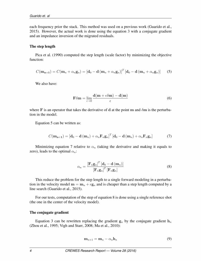
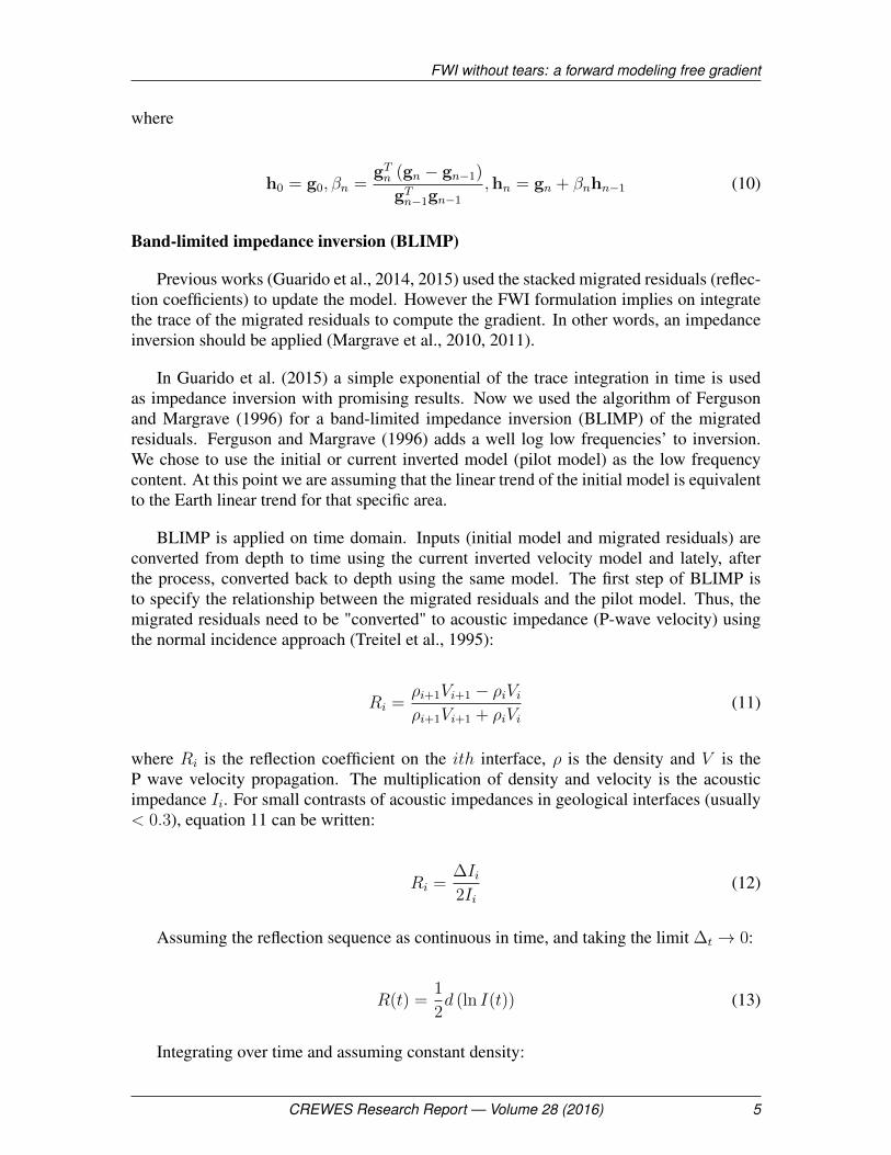
The synthetic test is done in the Marmousi model (figure 1). Pilot shots (used as thereal shots), were created using an acoustic finite difference algorithm. In the total, 102shots are used to simulate field data. Shot spacing is 100m. Each shot has a maximumof 401 receivers (varying in the edges of the model) totalizing 2000m of maximum offset.The register time is 3s and sample rating of 4ms (figure 2). The dominant frequency of thewavelet is 5Hz.

During the FWI routine, synthetic shots are created with the same finite difference for-ward modeling algorithm, wavelet and acquisition parameters as pilot shots. They differfrom each other by the velocity model used and the routine starts using a guessing model,usually a depth migration velocity (Virieux and Operto, 2009). The residuals (difference



FIG. 1. The Marmousi 2D model. The color bar indicates the wave propagation velocity in m/s.

FIG. 2. Three of the 102 shots used in the test. a) shot 3, b) shot 52 and c) shot 102.

between real and synthetic shot) is then migrated with the PSPI migration with a decon-volution imaging condition. For the first iterations, only very low frequencies are used(4 − 6Hz), and the range is increased by 2Hz when errors are stable (variation of the 3last iterations is less than 0.1%). Each residual is migrated separately using the initial orupdated model. A mute is applied before stacking the migrated residuals (Guarido et al.,2014) and the stack is preconditioning by convolving it with a 2D Gaussian window (Mar-grave et al., 2010; Guarido et al., 2014). Ferguson and Margrave (1996)’s algorithm forimpedance inversion is used after the conjugate gradient step. Lately the step length isestimated using equation 8 and the model is updated for the next iteration.

Initial model as well control

BLIMP is applied on the migrated residuals to estimate the gradient and the modelupdate expecting to compensate the lack of low frequencies on the data (seismic lowestfrequency used is 4Hz) following those steps:

• Residuals are computed as the difference between synthetic and acquired seismic


Guarido et. al

shots.

• Each residual is depth migrated using the PSPI algorithm with a deconvolution imag-ing condition.

• The migrated residuals are muted and stacked to form a pseudo-gradient.

• The pseudo-gradient and current model are stretched from depth to time.

• BLIMP is applied on the pseudo-gradient using the current model’s low frequency toform the gradient in time.

• Gradient is stretched from time to depth using current model.

• Step length is computed using equation 8.

• Model is updated using the scaled gradient.

Even if we compute a gradient that points on the opposite direction to the global mini-mum and estimate a step length to converge faster to the same point, the gradient descentmethod is known to get "trapped" on a local minimum (Pratt et al., 1998). One way to min-imize this effect is to start the inversion with very low frequencies (multi-scale approach).Another way is to start the inversion closer to the global minimum (a good initial model).

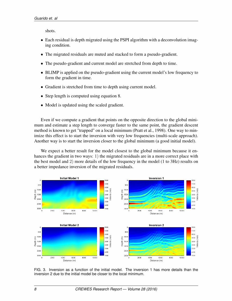
We expect a better result for the model closest to the global minimum because it en-hances the gradient in two ways: 1) the migrated residuals are in a more correct place withthe best model and 2) more details of the low frequency in the model (1 to 3Hz) results ona better impedance inversion of the migrated residuals.

FIG. 3. Inversion as a function of the initial model. The inversion 1 has more details than theinversion 2 due to the initial model be closer to the local minimum.



Figure 3 illustrates the different inversions with varying qualities of the initial model.In both cases, the multi-scale approach is implemented. When the starting point is closerto the global minimum, the inversion leads to a higher resolution resulting model (Guaridoet al., 2015). In both cases, it is noticeable of how much information is included to themodel. Most of the features from low to mid frequencies were successfully recovered.The faults with high dip angle in the shallow (central portion of the model) are present onboth inversions. Even the simulation of a gas anomaly (x = 6500, z = 2500) could beinterpreted for the inversion with the best initial model.

The algorithm worked successfully for low to mid frequencies (up to 16Hz) and had noupdates on higher frequencies (the gradient exists but the step length goes to zero, meaningthat the inversion was too close to a minimum point).

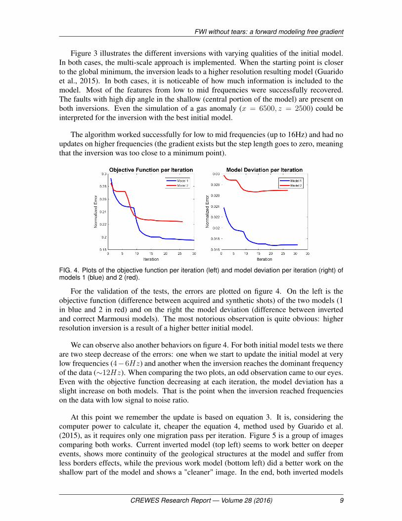
FIG. 4. Plots of the objective function per iteration (left) and model deviation per iteration (right) ofmodels 1 (blue) and 2 (red).

For the validation of the tests, the errors are plotted on figure 4. On the left is theobjective function (difference between acquired and synthetic shots) of the two models (1in blue and 2 in red) and on the right the model deviation (difference between invertedand correct Marmousi models). The most notorious observation is quite obvious: higherresolution inversion is a result of a higher better initial model.

We can observe also another behaviors on figure 4. For both initial model tests we thereare two steep decrease of the errors: one when we start to update the initial model at verylow frequencies (4−6Hz) and another when the inversion reaches the dominant frequencyof the data (∼12Hz). When comparing the two plots, an odd observation came to our eyes.Even with the objective function decreasing at each iteration, the model deviation has aslight increase on both models. That is the point when the inversion reached frequencieson the data with low signal to noise ratio.

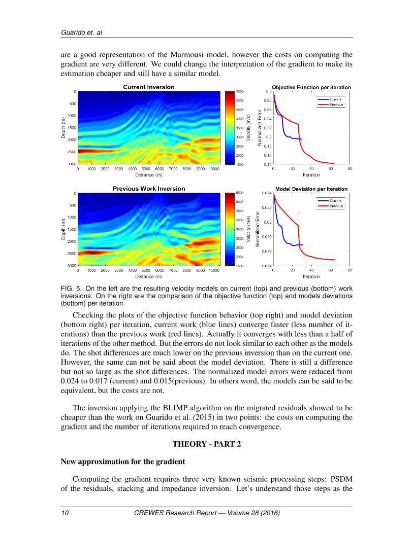
At this point we remember the update is based on equation 3. It is, considering thecomputer power to calculate it, cheaper the equation 4, method used by Guarido et al.(2015), as it requires only one migration pass per iteration. Figure 5 is a group of imagescomparing both works. Current inverted model (top left) seems to work better on deeperevents, shows more continuity of the geological structures at the model and suffer fromless borders effects, while the previous work model (bottom left) did a better work on theshallow part of the model and shows a "cleaner" image. In the end, both inverted models


Guarido et. al

are a good representation of the Marmousi model, however the costs on computing thegradient are very different. We could change the interpretation of the gradient to make itsestimation cheaper and still have a similar model.

FIG. 5. On the left are the resulting velocity models on current (top) and previous (bottom) workinversions. On the right are the comparison of the objective function (top) and models deviations(bottom) per iteration.

Checking the plots of the objective function behavior (top right) and model deviation(bottom right) per iteration, current work (blue lines) converge faster (less number of it-erations) than the previous work (red lines). Actually it converges with less than a half ofiterations of the other method. But the errors do not look similar to each other as the modelsdo. The shot differences are much lower on the previous inversion than on the current one.However, the same can not be said about the model deviation. There is still a differencebut not so large as the shot differences. The normalized model errors were reduced from0.024 to 0.017 (current) and 0.015(previous). In others word, the models can be said to beequivalent, but the costs are not.

The inversion applying the BLIMP algorithm on the migrated residuals showed to becheaper than the work on Guarido et al. (2015) in two points: the costs on computing thegradient and the number of iterations required to reach convergence.

THEORY - PART 2

New approximation for the gradient

Computing the gradient requires three very known seismic processing steps: PSDMof the residuals, stacking and impedance inversion. Let’s understand those steps as the



operators M for migration, S for stacking and I for impedance inversion. Equation 3 can bere-written as:

mn+1 = mn − αngn= mn − αnI {S [M (∆d(mn))]}= mn − αnI {S [M (d0 − d(mn))]} (18)

where ∆d(mn) is the n-th iteration residual d0 − d(mn), d0 is the acquired data, d(mn)is the synthetic data of the n-th iteration and mn is the n-th iteration inverted model. Forsimplification and easier visualization, let’s set d(mn) = dn. Then equation 18 is:

mn+1 = mn − αnI {S [M (d0 − dn)]} (19)

Considering the linearity property of the migration operator (see appendix), the ac-quired and synthetic shots can be migrated separately:

mn+1 = mn − αnI {S [M (d0)−M (dn)]} (20)

The next step is to use the linearity property of the stacking operator and equation 20becomes:

mn+1 = mn − αnI {S [M (d0)]− S [M (dn)]} (21)

For the impedance inversion operator, the first approximation we tried is I(x1 − x2) =

I0I(x1)I(22)

. Then equation 21 can be written as:

mn+1 = mn − αnI0I {S [M (d0)]}I {S [M (dn)]}︸︷︷︸

Current model

(22)

where the denominator is the impedance inversion of the stacked depth migrated syntheticshots should be the velocity model on which the forward modeling algorithm is ran into. Inothers words, it is the model of the current iteration mn. Then equation 25 can be simplifiedto:

mn+1 = mn − αnI0I {S [M (d0)]}

mn

(23)

Equation 23 shows to be unstable as it can be divided by zero (as we are inverting forlower frequencies greater than 3Hz and not capturing the Earth linear trend, it can result on


Guarido et. al

zeros and even negative impedance). Trying to avoid this we added a stabilization factorSF:

mn+1 = mn − αnI0I {S [M (d0)]}

mn + SF(24)

Choosing a value for the stabilization factor showed to be challenging. A too smallvalue can lead areas of the gradient to have a huge value compared with its neighbors. Alarge value (around 1 and above) can change the denominator significantly. And the valueneeded to be changed at each iteration by trial and error. Avoiding the division of equation24 is the best tactic at this point. So we took the risk to say that the impedance inversionoperator is approximately linear (for that, we assume Earth impedance to follow a lineartrend and a Taylor expansion of the reflection coefficients is used to estimate the update asa perturbation of Earth’s impedance), we end up with another solution for equation 21:

mn+1 = mn − αn(I {S [M (d0)]} − I {S [M (dn)]}︸︷︷︸Current model

) (25)

Again, on the second hand of the gradient approximation we have the model of thecurrent iteration mn. Then equation 25 is simplified to:

mn+1 = mn + αn(I {S [M (d0)]} −mn) (26)

Equations 26 and 24 understand the gradient as a residual impedance inversion of theacquired data relative to the current model. This is an impressive result as no forwardmodeling or source estimation is required to compute the gradient. The objective functionis being minimized on the estimation of the step length (that requires 2 synthetic data: onefor the current model and one for a gradient perturbation of the same model). On ourMarmousi tests, we reduced, per iteration, the need of 105 forward modeling runs to only2. Actually, the amount of forward modelings required for any project does not depend onhow many shots it has, but on how many control points for the step length estimation theprocessor wants to use.

RESULTS - PART 2

Pre-stack depth migration based gradient

Equations 26 and 24 reduced abruptly the computer power required for the inversion.From now on, all the tests were done on a personal gaming laptop (ASUS Intel Core i7-4700HQ 2.40GHz, 4 cores, 16Gb of Ram memory) in Octave (free scripting software) ona Linux terminal and no parallel processing.

Figure 6 shows the inversion based on equation 26, starting from the model on the topleft of figure 3 and with the computer specification cited previously. The result is impressive



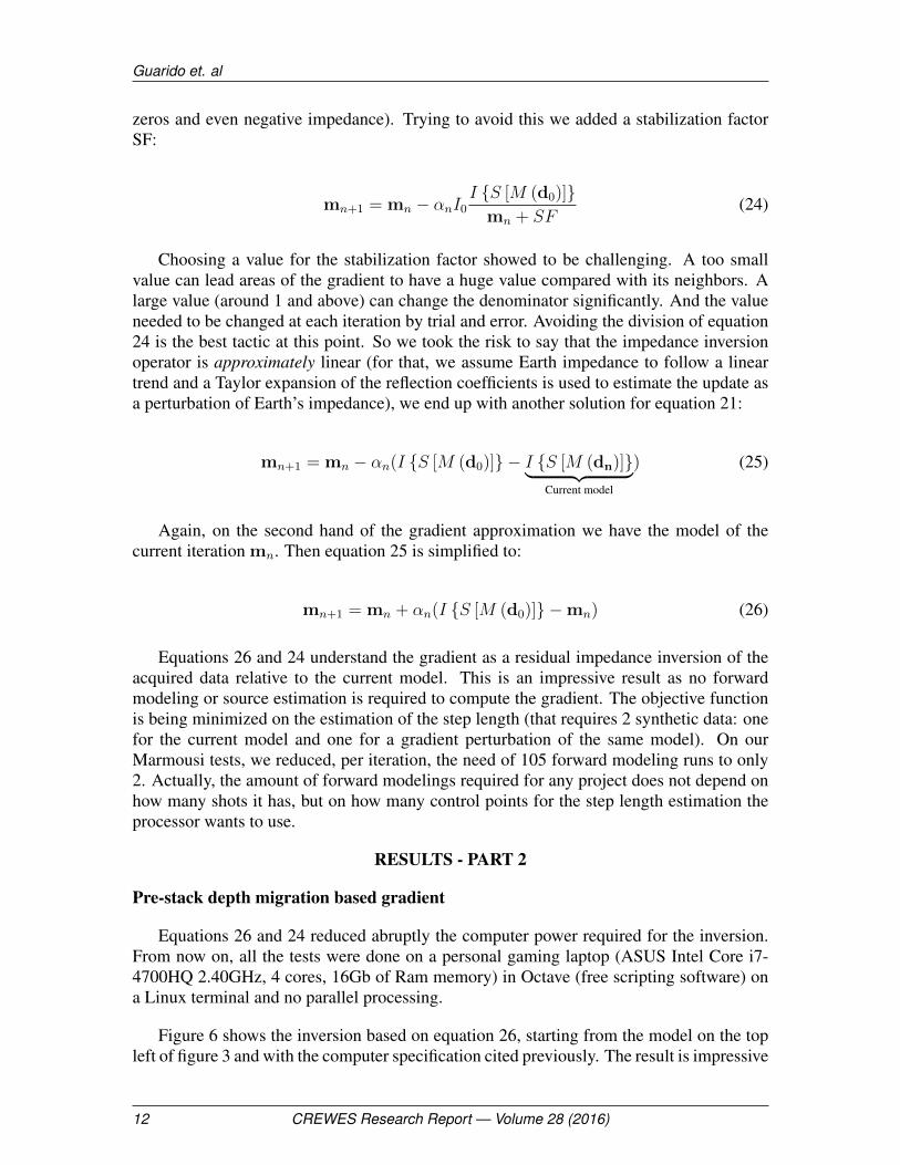
FIG. 6. Inverted model using the initial model on the top left of figure 3 and based on equation 26.The algorithm ran on a personal laptop without the need of parallel processing in about 36 hours.

and the process stopped after 29 iterations in about 36 hours of run time with no parallelprocessing (it was repeated using the 4 cores of the computer for parallel processing andelapsed time decreased to 18 hours). The method worked well in the whole model butbetter at shallower areas. Major structures are successfully inverted. Even the fault zonesin the center of the model can be interpreted. Using any forward modeling to computethe gradient shows to be a valid approximation. BLIMP provides us an impedance modelwhich includes the perturbation (high frequency) of the impedance to the low frequencymodel. The difference of the perturbations of current and previous iterations (the proposedgradient) points to the correct minimum but is not optimized to minimize the objectivefunction of equation 1. The step length (that requires 2 forward modeling per iteration tobe estimated) works as the minimization operator. The conjugate gradient was not used(we tested with and without it and the ending models were equivalent).

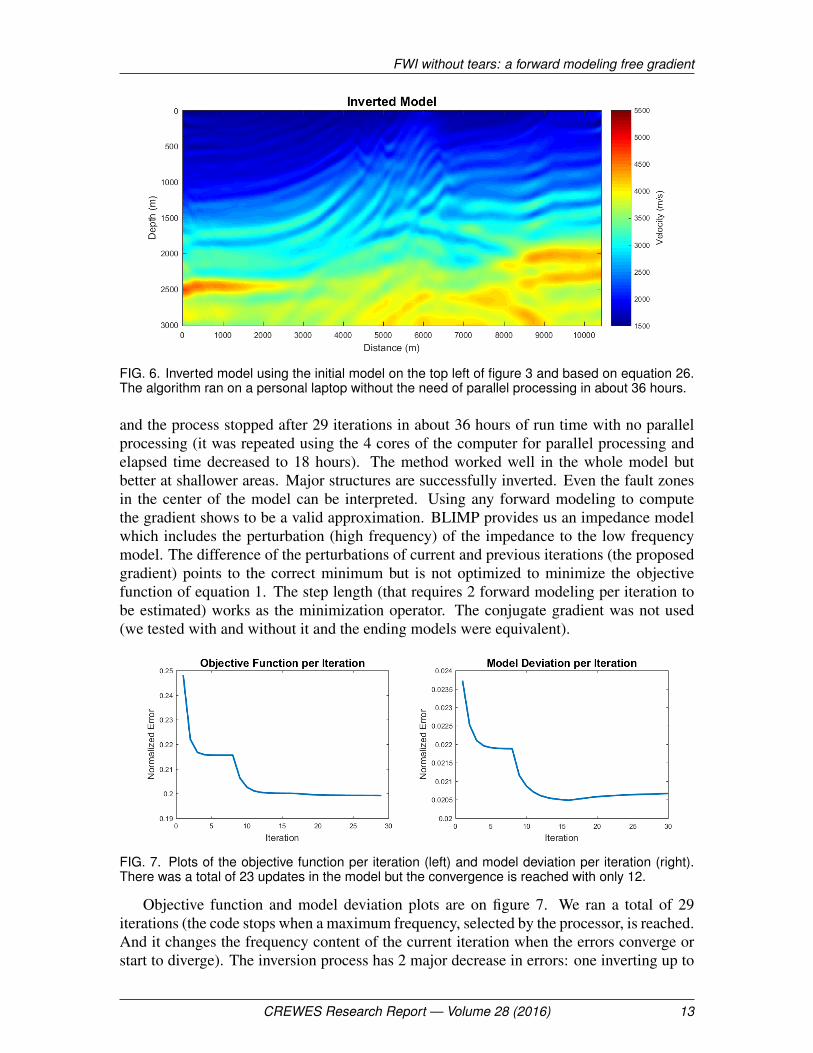
FIG. 7. Plots of the objective function per iteration (left) and model deviation per iteration (right).There was a total of 23 updates in the model but the convergence is reached with only 12.

Objective function and model deviation plots are on figure 7. We ran a total of 29iterations (the code stops when a maximum frequency, selected by the processor, is reached.And it changes the frequency content of the current iteration when the errors converge orstart to diverge). The inversion process has 2 major decrease in errors: one inverting up to


Guarido et. al

6Hz and another up to 10Hz. We believe those are the dominant frequencies related to thewavelength as same "size" of layers in the model. It is interesting to note that even with theobjective function keeps decreasing by iteration, the model deviation can diverge at somepoint (close to iteration 17). The meaning is that the process is trapped on a local minimumof the objective function that changed direction of the optimized model for it. With allthese information in mind, we can say the method is stable and leads to a optimized modelgets closer to the real one when minimizing the objective function.

Post-stack depth migration based gradient

Looking again at equation 26, we understand we are estimating the gradient by applyingsome seismic processing tools. If we think about migration and stack, migrating the dataand stacking should have the same effect as doing the inverted process (stack then migrate).Then equation 26 is equivalent to:

mn+1 = mn + αn(I {M [S (d0)]} −mn) (27)

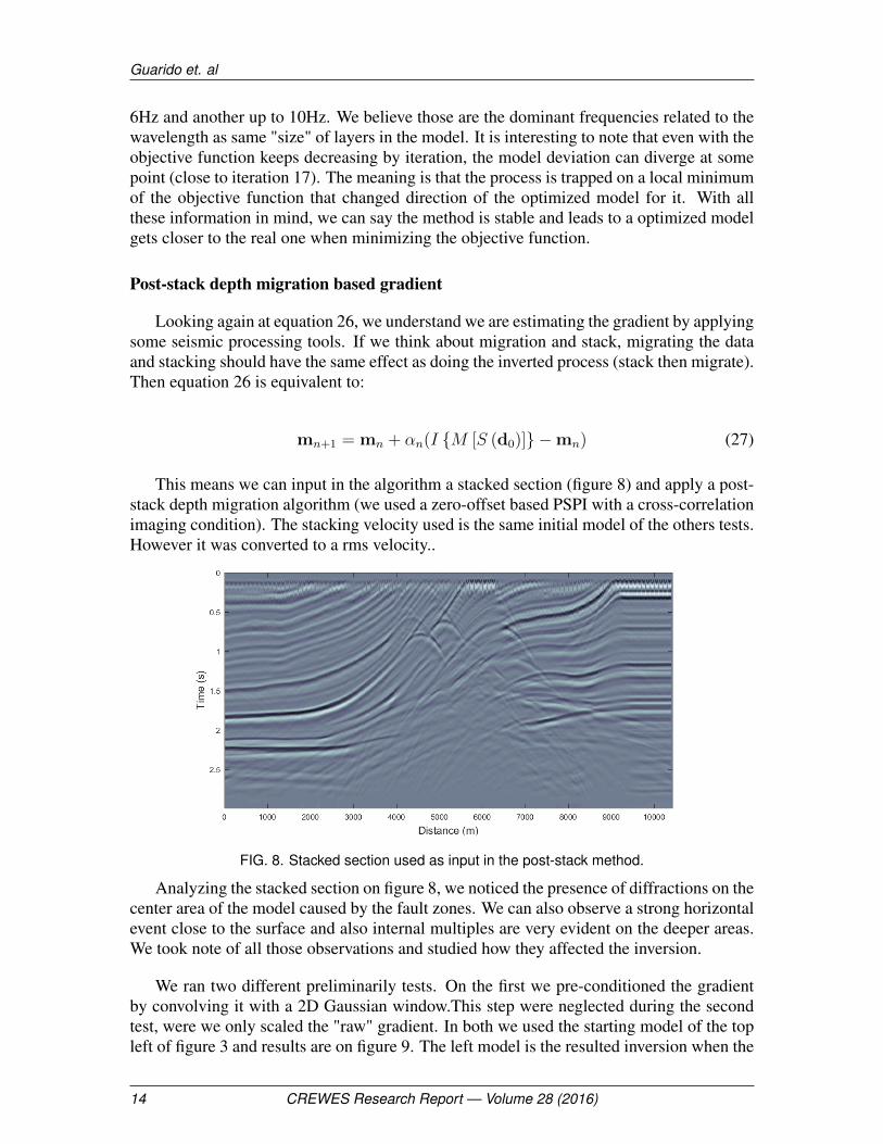
This means we can input in the algorithm a stacked section (figure 8) and apply a post-stack depth migration algorithm (we used a zero-offset based PSPI with a cross-correlationimaging condition). The stacking velocity used is the same initial model of the others tests.However it was converted to a rms velocity..

FIG. 8. Stacked section used as input in the post-stack method.

Analyzing the stacked section on figure 8, we noticed the presence of diffractions on thecenter area of the model caused by the fault zones. We can also observe a strong horizontalevent close to the surface and also internal multiples are very evident on the deeper areas.We took note of all those observations and studied how they affected the inversion.

We ran two different preliminarily tests. On the first we pre-conditioned the gradientby convolving it with a 2D Gaussian window.This step were neglected during the secondtest, were we only scaled the "raw" gradient. In both we used the starting model of the topleft of figure 3 and results are on figure 9. The left model is the resulted inversion when the



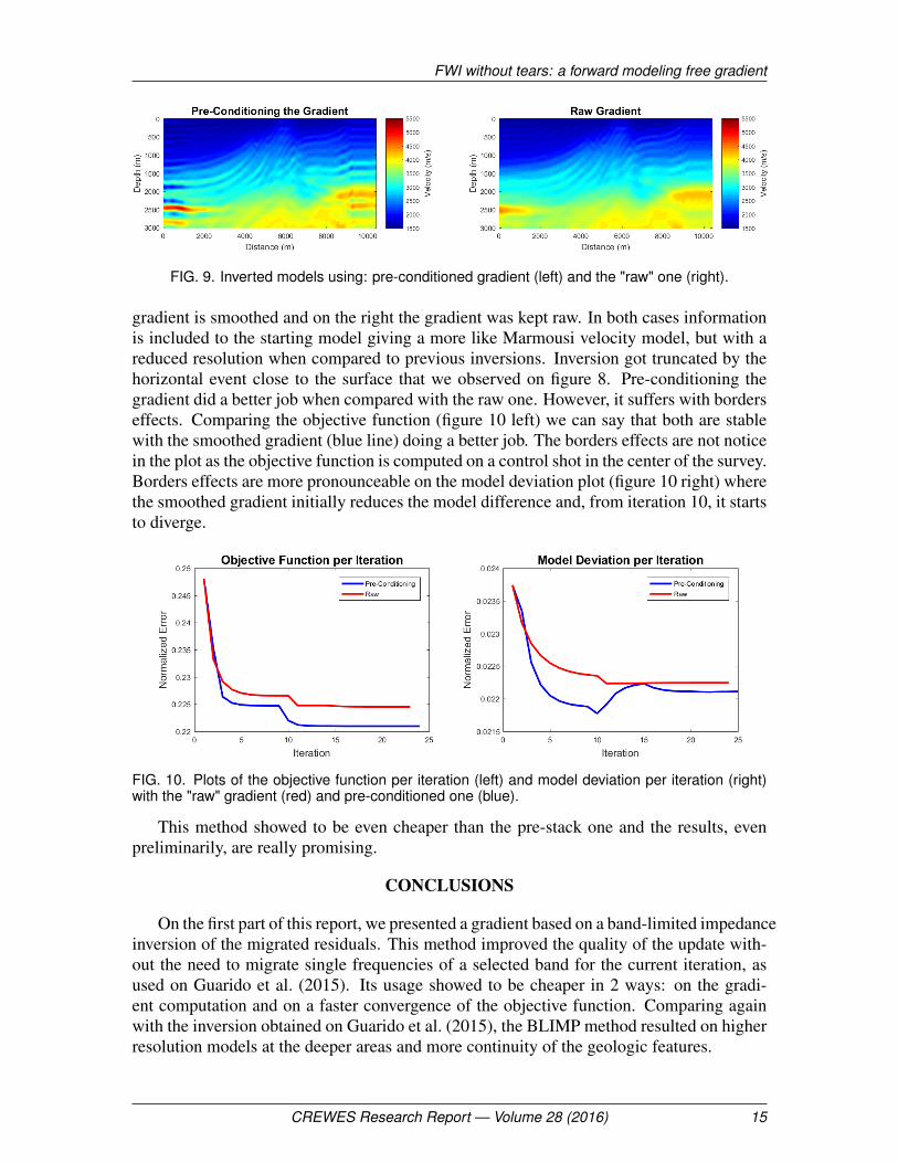
FIG. 9. Inverted models using: pre-conditioned gradient (left) and the "raw" one (right).

gradient is smoothed and on the right the gradient was kept raw. In both cases informationis included to the starting model giving a more like Marmousi velocity model, but with areduced resolution when compared to previous inversions. Inversion got truncated by thehorizontal event close to the surface that we observed on figure 8. Pre-conditioning thegradient did a better job when compared with the raw one. However, it suffers with borderseffects. Comparing the objective function (figure 10 left) we can say that both are stablewith the smoothed gradient (blue line) doing a better job. The borders effects are not noticein the plot as the objective function is computed on a control shot in the center of the survey.Borders effects are more pronounceable on the model deviation plot (figure 10 right) wherethe smoothed gradient initially reduces the model difference and, from iteration 10, it startsto diverge.

FIG. 10. Plots of the objective function per iteration (left) and model deviation per iteration (right)with the "raw" gradient (red) and pre-conditioned one (blue).

This method showed to be even cheaper than the pre-stack one and the results, evenpreliminarily, are really promising.

CONCLUSIONS

On the first part of this report, we presented a gradient based on a band-limited impedanceinversion of the migrated residuals. This method improved the quality of the update with-out the need to migrate single frequencies of a selected band for the current iteration, asused on Guarido et al. (2015). Its usage showed to be cheaper in 2 ways: on the gradi-ent computation and on a faster convergence of the objective function. Comparing againwith the inversion obtained on Guarido et al. (2015), the BLIMP method resulted on higherresolution models at the deeper areas and more continuity of the geologic features.


Guarido et. al

Second, we presented a new interpretation of the gradient that is forward modeling andsource estimation free. We understand the gradient to be a residual impedance inversionof the acquired data. It is stable, converge fast and is impressively cheap, as the inversionwas done on a personal laptop without parallel processing. Two forward modelings arestill required on the step length estimation. The resulting model contains all the biggerstructures of the Marmousi model, as the inversion worked well on low frequencies up to6Hz. The model converged early due to a horizontal artifact close to the surface. Immediatefuture work is to suppress such artifact and allow higher frequencies to be included in theinverted model as well.

Following the forward modeling free gradient and understanding the FWI algorithm asa combination of different seismic processing tools, we inverted the order of the migrationand stacking operators and applied a post-stack depth migration (zero offset PSPI) on astack section. The results are preliminarily but really promising.

In the end we came with a cheap solution to apply an acoustic FWI with promisingresults and we are confident that the same approximation can be extended to others param-eters.

ACKNOWLEDGMENTS

The authors thank the sponsors of CREWES for continued support. This work wasfunded by CREWES industrial sponsors and NSERC (Natural Science and EngineeringResearch Council of Canada) through the grant CRDPJ 461179-13. We thank Soane Motados Santos for the suggestions, tips and productive discussions.

REFERENCES

Bishop, T. N., and Spongberg, M. E., 1984, Seismic tomography: A case study: SEG Technical ProgramExpanded Abstracts, 313, 712–713.

Chipman, J. S., 1999, Linear restrictions, rank reduction, and biased estimation in linear regression: LinearAlgebra and its Applications, 289, No. 1, 55 – 74.

Claerbout, J. F., 1971, Toward a unifeid theory of reflection mapping: Geophysics, 36, No. 3, 467–481.

Cutler, R. T., Bishop, T. N., Wyld, H. W., Shuey, R. T., Kroeger, R. A., Jones, R. C., and Rathbun, M. L.,1984, Seismic tomography: Formulation and methodology: SEG Technical Program Expanded Abstracts,312, 711–712.

Fatti, J. L., Smith, G. C., Vail, P. J., Strauss, P. J., and Levitt, P. R., 1994, Detection of gas in sandstonereservoirs using avo analysis: A 3-d seismic case history using the geostack technique: Geophysics, 59,No. 9, 1362–1376.

Ferguson, R., and Margrave, G., 2005, Planned seismic imaging using explicit one-way operators: Geo-physics, 70, No. 5, S101–S109.

Ferguson, R. J., and Margrave, G., 1996, A simple algorithm for band-limited impedance inversion:CREWES Research Report, 83, 21.1–21.10.

Guarido, M., Lines, L., and Ferguson, R., 2014, Full waveform inversion - a synthetic test using the pspimigration: CREWES Research Report, 26, 26.1–26.23.

Guarido, M., Lines, L., and Ferguson, R., 2015, Full waveform inversion: a synthetic test using pspi migra-tion: SEG Technical Program Expanded Abstract, 279, 1456–1460.



Lailly, P., 1983, The seismic inverse problem as a sequence of before stack migrations: Conference on inversescattering, theory and application: Society of Industrial and Applied Mathematics, Expanded Abstracts,206–220.

Langan, R. T., Lerche, I., Cutler, R. T., Bishop, T. N., and Spera, N. J., 1984, Seismic tomography: Theaccurate and efficient tracing of rays through heterogeneous media: SEG Technical Program ExpandedAbstracts, 314, 713–715.

Lindseth, R. O., 1979, Synthetic sonic logs-a process for stratigraphic interpretation: Geophysics, 44, No. 1,3–26.

Ma, Y., Hale, D., Meng, Z. J., and Gong, B., 2010, Full waveform inversion with image-guided gradient:SEG Technical Program Expanded Abstracts, 198, 1003–1007.

Margrave, G., Ferguson, R., and Hogan, C., 2010, Full waveform inversion with wave equation migrationand well control: CREWES Research Report, 22, 63.1–63.20.

Margrave, G., Yedlin, M., and Innanen, K., 2011, Full waveform inversion and the inverse hessian: CREWESResearch Report, 23, 77.1–77.13.

Pica, A., Diet, J. P., and Tarantola, A., 1990, Nonlinear inversion of seismic reflection data in a laterallyinvariant medium: Geophysics, 55, No. 2, R59–R80.

Pratt, R. G., Shin, C., and Hick, G. J., 1998, Gauss-newton and full newton methods in frequency-spaceseismic waveform inversion: Geophysical Journal International, 133, No. 2, 341–362.

Shuey, R. T., 1985, A simplification of the zoeppritz equations: Geophysics, 50, No. 4, 609–614.

Tarantola, A., 1984, Inversion of seismic reflection data in the acoustic approximation: Geophysics, 49, No. 8,1259–1266.

Treitel, S., Lines, L., and Ruckgaber, G., 1995, Seismic impedance estimation: Geophysical Inversion andApplications - Memorial University of Newfoundland, 1, 6–11.

Vigh, D., and Starr, E. W., 2008, 3d prestack plane-wave, full-waveform inversion: GEOPHYSICS, 73, No. 5,VE135–VE144.

Virieux, J., and Operto, S., 2009, An overview of full-waveform inversion in exploration geophysics: Geo-physics, 74, No. 6, WCC1–WCC26.

Warner, M., and Guasch, L., 2014, Adaptive waveform inversion: Theory: SEG Technical Program ExpandedAbstracts, 207, 1089–1093.

Waters, K. H., 1978, Reflection seismology: John Wiley and Sons.

Wenyong, P., Margrave, G., and Innanen, K., 2013, On the role of the deconvolution imaging condition infull waveform inversion: CREWES Research Report, 25, 72.1–72.19.

Zhou, C., Cai, W., Luo, Y., Schuster, G. T., and Hassanzadeh, S., 1995, Acoustic wave-equation traveltimeand waveform inversion of crosshole seismic data: GEOPHYSICS, 60, No. 3, 765–773.


Guarido et. al

APPENDIX

Linearity of the migration operator

Claerbout (1971) suggests to map a reflection point (or layer) by a cross-correlation ofthe downgoing and upgoing wave fields:

Im(x, z) = g(x, z, t)⊗ u(x, z, t) (28)

where u(x, z, t) is the upgoing residuals wavefield dm − d0, dm is the synthetic data usingmodel m, d0 is the acquired data and g(x, z, t) is the downgoing source wavefield. Fromnow on we will omit the coordinates x and z on the notation and keep in mind that weare imaging in depth. In the frequency domain (after a Fourier Transform) equation 28becomes:

Im = U(ω)G∗(ω) (29)

where ∗ denotes the complex conjugate, U(ω) and G(ω) are the Fourier Transform of u(t)and g(t), respectively. The linear property of the Fourier Transform leads to U(ω) =Dm(ω)−D0(ω), where Dm(ω) and D0(ω) are the Fourier Transform of dm and d0, respec-tively. From equation 29:

Im = U(ω)G∗(ω)

= (Dm(ω)−D0(ω))G∗(ω)

= Dm(ω)G∗(ω)−D0(ω)G∗(ω)

Im(x, z) = g(x, z, t)⊗ dm(x, z, t)− g(x, z, t)⊗ d0(x, z, t) (30)

This means that applying the imaging condition of equation 28 on the residuals u isequivalent to subtract the imaging condition of d0 to the dm, proving the linearity propertyof the migration operator.

Linearity of the stacking operator

For a common imaging point of a seismic survey we have N traces trui of the residualstrui = trmi

− tr0i (i is the shot position or number, m relates the trace to the synthetic shotand 0 to the acquired data). Stacking them is:

Su =N∑i=1

truiN

(31)



Now solving the sum of the residual terms of equation 31 we demonstrate the linearproperty of stacking operator:

Su =N∑i=1

truiN

=N∑i=1

trmi− tr0iN

=1

N(trm1 − tr01 + trm2 − tr02 + · · ·+ trmN

− tr0N )

=1

N[trm1 + trm2 + · · ·+ trmN

− (tr01 + tr02 + · · ·+ tr0N )]

=1

N(N∑i=1

trmi−

N∑i=1

tr0i)

= Sm − S0 (32)

Linearity approximation of the impedance inversion operator

Another way to re-write the reflection coefficients R and impedances I of equation 11is given by Treitel et al. (1995) for the reflection at point k is:

Ik = I0

N∏k=1

(1 +Rk

1−Rk

)(33)

The next step to to apply a Taylor expansion on the denominator. But first let’s under-stand on the values the reflection coefficient can be. A strong water bottom reflector (watervelocity = 1500m/s and first layer velocity = 2100m/s) would have a reflection coefficientof around 0.21 and the squared of it is 0.04. On a "well behaved" Earth, besides the waterbottom and high impedance layers as salt or basalt, the reflection coefficients have valuesof around 0.03 or less, which squared would be 0.0007 and less. We came to this analysisso terms of power 2 and higher on the Taylor expansion and products can be neglected.With this information in mind, equation 33 is:

Ik = I0

N∏k=1

[(1 +Rk)(1 +Rk +R2

k +R3k + · · · )

]≈ I0

N∏k=1

[(1 +Rk)(1 +Rk)] (34)

Equation 34 leads to an easier solution for the impedance. Now we can open the productand, as previously, neglect powers 2 and higher of the reflection coefficients:


Guarido et. al

Ik = I0

N∏k=1

(1 + 2Rk +R2k)

≈ I0

N∏k=1

(1 + 2Rk)

= I0(1 + 2R1)(1 + 2R2)(1 + 2R3) · · · (1 + 2RN)

= I0(1 + 2R1 + 2R2 + 2R3 · · · 2RN +O(power ≥ 2))

= I0(1 + 2N∑k=1

Rk) (35)

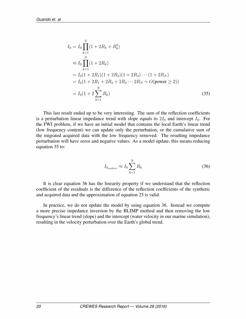
This last result ended up to be very interesting. The sum of the reflection coefficientsis a perturbation linear impedance trend with slope equals to 2I0 and intercept I0. Forthe FWI problem, if we have an initial model that contains the local Earth’s linear trend(low frequency content) we can update only the perturbation, or the cumulative sum ofthe migrated acquired data with the low frequency removed. The resulting impedanceperturbation will have zeros and negative values. As a model update, this means reducingequation 35 to:

Ikupdate ≈ I0

N∑k=1

Rk (36)

It is clear equation 36 has the linearity property if we understand that the reflectioncoefficient of the residuals is the difference of the reflection coefficients of the syntheticand acquired data and the approximation of equation 25 is valid.

In practice, we do not update the model by using equation 36. Instead we computea more precise impedance inversion by the BLIMP method and then removing the lowfrequency’s linear trend (slope) and the intercept (water velocity in our marine simulation),resulting in the velocity perturbation over the Earth’s global trend.


Documents

FWI without tears: a forward modeling free gradient · FWI without tears: a forward modeling free gradient is required on its estimation. The results are comparable with the classic