Fuzzy Systems - Fuzzy Rule Basesfuzzy.cs.ovgu.de/ci/fs/fs_ch06_frb.pdf · Fuzzy Systems Fuzzy Rule Bases Prof. Dr. Rudolf Kruse Christian Moewes {kruse,cmoewes}@iws.cs.uni-magdeburg.de

$Page 1: Fuzzy Systems - Fuzzy Rule Basesfuzzy.cs.ovgu.de/ci/fs/fs_ch06_frb.pdf · Fuzzy Systems Fuzzy Rule Bases Prof. Dr. Rudolf Kruse Christian Moewes {kruse,cmoewes}@iws.cs.uni-magdeburg.de$
Fuzzy SystemsFuzzy Rule Bases

Prof. Dr. Rudolf Kruse Christian Moewes{kruse,cmoewes}@iws.cs.uni-magdeburg.de

Otto-von-Guericke University of MagdeburgFaculty of Computer Science

Department of Knowledge Processing and Language Engineering

R. Kruse, C. Moewes FS – Fuzzy Rule Bases Lecture 6 1 / 43

http://fuzzy.cs.ovgu.de/wiki/pmwiki.php?n=Mitarbeiter.Kruse

http://fuzzy.cs.ovgu.de/wiki/pmwiki.php?n=Mitarbeiter.Moewes

http://www.ovgu.de/

http://www.fin.ovgu.de/

http://iws.cs.ovgu.de/

mailto:[email protected]


Outline

1. Fuzzy Control

Example: Cartpole Problem

Fuzzy Approach

Fuzzy Controller

Architecture of a Fuzzy Controller

2. Fuzzy Rule Bases

Example – Parking a car backwards

Questions:

What is the meaning of satisfactory parking?

Demand on precision?

Realization of control?




Fuzzy Control

Biggest success of fuzzy systems in industry and commerce.

Special kind of non-linear table-based control method.

Definition of non-linear transition function can be made withoutspecifying each entry individually.

Examples: technical systems

• Electrical engine moving an elevator,

• Heating installation

Goal: define certain behavior

• Engine should maintain certain number of revolutions per minute.

• Heating should guarantee certain room temperature.




Table-based Control

Control systems all share a time-dependent output variable:

• Revolutions per minute,

• Room temperature.

Output is controlled by control variable:

• Adjustment of current,

• Thermostat.

Also, disturbance variables influence output:

• Load of elevator, . . . ,

• Outside temperature or sunshine through a window, . . .




Table-based Control

Computation of actual value incorporates both

control variable measurements of current output variable ξ and

change of output variable ∆ξ = dξdt

.

If ξ is given in finite time intervals,

then set ∆ξ(tn+1) = ξ(tn+1) − ξ(tn).

In this case measurement of ∆ξ not necessary.




Example: Cartpole Problem

MF

θ

l

m

g

Balance an upright standing pole by moving itsfoot.

Lower end of pole can be moved unrestrained alonghorizontal axis.

Mass m at foot and mass M at head.

Influence of mass of shaft itself is negligible.

Determine force F (control variable) that isnecessary to balance pole standing upright.

That is measurement of following output variables:

• angle θ of pole in relation to vertical axis,

• change of angle, i.e. triangular velocity θ = dθdt

.

Both should converge to zero.




Notation

Input variables ξ1, . . . , ξn, control variable η

Measurements: used to determine actual value of η

η may specify change of η.

Assumption: ξi , 1 ≤ i ≤ n is value of Xi , η ∈ Y

Solution: control function ϕ

ϕ : X1 × . . . × Xn → Y

(x1, . . . , xn) 7→ y




Example: Cartpole Problem (cont.)

Angle θ ∈ X1 = [−90 ◦, 90 ◦]

Theoretically, every angle velocity θ possible.

Extreme θ are artificially achievable.

Assume −45 ◦/s ≤ θ ≤ 45 ◦/s holds,i.e. θ ∈ X2 = [−45 ◦/s, 45 ◦/s].

Absolute value of force |F | ≤ 10 N.

Thus define F ∈ Y = [−10 N, 10 N].





Differential equation of cartpole problem:

(M +m) sin2 θ · l · θ +m · l ·sin θ cos θ · θ2 −(M +m) ·g ·sin θ = −F ·cos θ

Compute F (t) such that θ(t) and θ(t) converge towards zero quickly.

Physical analysis demands knowledge about physical process.




Problems of Classical Approach

Often very difficult or even impossible to specify accuratemathematical model.

Description with differential equations is very complex.

Profound physical knowledge from engineer.

Exact solution can be very difficult.

Should be possible: to control process without physical-mathematicalmodel,e.g. human being knows how to ride bike without knowing existence ofdifferential equations.




Fuzzy Approach

Simulate behavior of human who knows how to control.

That is a knowledge-based analysis.

Directly ask expert to perform analysis.

Then expert specifies knowledge as linguistic rules, e.g. for cartpoleproblem:

“If θ is approximately zero and θ is also approximately zero,then F has to be approximately zero, too.”




Fuzzy Approach: Fuzzy Partitioning

1. Formulate set of linguistic rules:

Determine linguistic terms (represented by fuzzy sets).

X1, . . . , Xn and Y is partitioned into fuzzy sets.

Define p1 distinct fuzzy sets µ(1)1 , . . . , µ

(1)p1 ∈ F(X1) on set X1.

Associate linguistic term with each set.




Fuzzy Approach: Fuzzy Partitioning II

Of set X1 corresponds to interval [a, b] of real line, then

µ(1)1 , . . . , µ

(1)p1 ∈ F(X1) are triangular functions

µx0,ε : [a, b] → [0, 1]

x 7→ 1 − min{ε · |x − x0|, 1}.

If a < x1 < . . . < xp1 < b, only µ(1)2 , . . . , µ

(1)p1−1 are triangular.

Boundaries are treated differently.




Fuzzy Approach: Fuzzy Partitioning III

left fuzzy set:

µ(1)1 : [a, b] → [0, 1]

x 7→

{

1, if x ≤ x1

1 − min{ε · (x − x1), 1} otherwise

right fuzzy set:

µ(1)p1

: [a, b] → [0, 1]

x 7→

{

1, if xp1 ≤ x

1 − min{ε · (xp1 − x), 1} otherwise




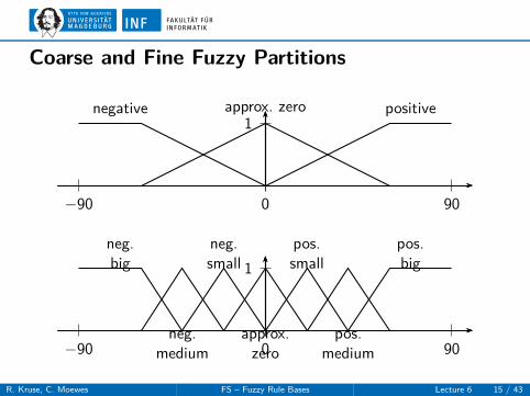
Coarse and Fine Fuzzy Partitions

1

0 90−90

negative approx. zero positive

1

0 90−90

neg.big

neg.medium

neg.small

approx.zero

pos.small

pos.medium

pos.big





X1 partitioned into 7 fuzzy sets.

Support of fuzzy sets: intervals with length 14 of whole range X1.

Similar fuzzy partitions for X2 and Y .

Next step: specify rules

if ξ1 is A(1) and . . . and ξn is A(n) then η is B,

A(1), . . . , A(n) and B represent linguistic terms corresponding toµ(1), . . . , µ(n) and µ according to X1, . . . , Xn and Y .

Rule base consists of k rules.





θnb nm ns az ps pm pb

nb ps pbnm pmns nm ns ps

θ az nb nm ns az ps pm pbps ns ps pmpm nmpb nb ns

19 rules for cartpole problem, e.g.

If θ is approximately zero and θ is negative mediumthen F is positive medium.




Fuzzy Approach: Challenge

How to define function ϕ : X → Y that fits to rule set?

Idea:

Represent set of rules as fuzzy relation.

Specify desired table-based controller by this fuzzy relation.




Fuzzy Relation

Consider only crisp sets.

Then, solving control problem = specifying control functionϕ : X → Y .

ϕ corresponds to relation

Rϕ = {(x , ϕ(x)) | x ∈ X} ⊆ X × Y .

For measured input x ∈ X , control value

{ϕ(x)} = {x} ◦ Rϕ.




Fuzzy Control Rules

If temperature is very high and pressure is slightly low,

then heat change should be slightly negative.

If rate of descent = positive big and airspeed = negative big andglide slope = positive big,

then rpm change = positive big and elevator angle change =insignificant change.




Architecture of a Fuzzy Controller I

controlledsystem

measuredvalues

controlleroutput

notfuzzy

notfuzzy

fuzzificationinterface fuzzy

decisionlogic fuzzy

defuzzificationinterface

knowledgebase




Architecture of a Fuzzy Controller II

Fuzzification interface• receives current input value (eventually maps it to suitable

domain),• converts input value into linguistic term or into fuzzy set.

Knowledge base (consists of data base and rule base)• Data base contains information about boundaries, possible

domain transformations, and fuzzy sets with correspondinglinguistic terms.

• Rule base contains linguistic control rules.

Decision logic (represents processing unit)• computes output from measured input accord. to knowledge base.

Defuzzification interface (represents processing unit)• determines crisp output value

(and eventually maps it back to appropriate domain).R. Kruse, C. Moewes FS – Fuzzy Rule Bases Lecture 6 22 / 43



Outline

1. Fuzzy Control

2. Fuzzy Rule Bases

Approximate Reasoning

Disjunctive Rules

Conjunctive Rules

Fuzzy Relational Equations

Approximate Reasoning with Fuzzy Rules

General schema

Rule 1: if X is M1, then Y is N1

Rule 2: if X is M2, then Y is N2...

...Rule r : if X is Mr , then Y is Nr

Fact: X is M ′

Conclusion: Y is N ′

Given r if-then rules and fact “X is M ′”, we conclude “Y is N ′”.

Typically used in fuzzy controllers.




Approximate ReasoningDisjunctive Imprecise Rule

Imprecise rule: if X = [3, 4] then Y = [5, 6].

Interpretation: values coming from [3, 4] × [5, 6].

X

Y

3 4

5

6




Approximate ReasoningDisjunctive Imprecise Rules

Several imprecise rules: if X = M1 then Y = N1,if X = M2 then Y = N2, if X = M3 then Y = N3.

Interpretation: rule 1 as well as rule 2 as well as rule 3 hold true.

X

Y

M1

M2

M3

N1

N2

N3

S =⋃r

i=1 Mi × Ni

“patchwork rug” describingfunction’s behavior as

indicator function




Approximate Reasoning: Conclusion

X

Y

output B

input x0

{x0} ◦ S = B




Approximate ReasoningDisjunctive Fuzzy Rules

one fuzzy rule:if X = nm then Y = ps

x

y

R

µnm

νps

R = µnm × νps

several fuzzy rules:ns → ns’, az → az’, ps → ps’

x

y

R

µns

νns

µaz

νaz

µps

νps

R = µns × νns’ ∪

µaz × νaz’ ∪ µps × νps’




Approximate Reasoning: ConclusionDisjunctive Fuzzy Rules

R

input

output

x0

3 fuzzy rules.

Every pyramid is specified by 1 fuzzy rule (Cartesian product).

Input x0 leads to gray-shaded fuzzy output {x0} ◦ R.R. Kruse, C. Moewes FS – Fuzzy Rule Bases Lecture 6 28 / 43



Disjunctive or Conjunctive?

Fuzzy relation R employed in reasoning is obtained as follows.

For each rule i , we determine relation Ri by

Ri(x , y) = min[Mi(x), Ni (y)]

for all x ∈ X , y ∈ Y .

Then, R is defined by union of Ri , i.e.

R =⋃

1≤i≤r

Ri .

That is, if-then rules are treated disjunctive.

If-then rules can be also treated conjunctive by

R =⋂

1≤i≤r

Ri .




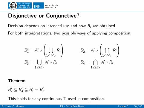
Disjunctive or Conjunctive?

Decision depends on intended use and how Ri are obtained.

For both interpretations, two possible ways of applying composition:

B′1 = A′ ◦

⋃

1≤i≤r

Ri

B′2 = A′ ◦

⋂

1≤i≤r

Ri

B′3 =

⋃

1≤i≤r

A′ ◦ Ri B′4 =

⋂

1≤i≤r

A′ ◦ Ri

Theorem

B′2 ⊆ B′

4 ⊆ B′1 = B′

3

This holds for any continuous ⊤ used in composition.




Approximate ReasoningConjunctive Imprecise Rules

if X = [3, 4] then Y = [5, 6]

Gray-shaded values are impossible, white ones are possible.

X

Y

3 4

5

6




Approximate ReasoningConjunctive Imprecise Rules

Several imprecise rules: if X = M1 then Y = N1,if X = M2 then Y = N2, if X = M3 then Y = N3.

X

Y

M1

M2

M3

N1

N2

N3 still possible are

R =⋂r

i=1(Mi × Ni ) ∪ (MCi × Y )

“corridor” describing

function’s behavior




Approximate Reasoning with Crisp Input

X

Y

R

possibleoutput

x0

output = {x0} ◦ R




Generalization to Fuzzy Rules

if X is approx. 2.5 then Y is approx. 5.5

0

0.25

0.50

0.75

1.00

1 2 3 4 x

µ(x)

0

0.25

0.50

0.75

1.00

4 5 6 7 y

ν(y)




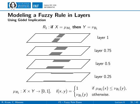
Modeling a Fuzzy Rule in LayersUsing Gödel Implication

R1 : if X = µM1then Y = νB1

layer 1

layer 0.75

layer 0.5

layer 0.25

µR1: X × Y → [0, 1], I(x , y) =

{

1 if µM1(x) ≤ νB1

(y),

νB1(y) otherwise.




Conjunctive Fuzzy Rule Base

R1 : if X = µM1then Y = νB1

, . . . , Rn : if X = µMnthen Y = νBn

...

layer 1

...

layer 0.25

µR = min1≤i≤r

µRi

Input µA, then output η with

η(y) = supx∈X

min {µA(x), µR (x , y)} .




Example: Fuzzy Relation

Classes of cars X = {s, m, h} (small, medium, high quality).

Possible maximum speeds Y = {140, 160, 180, 200, 220} (in km/h).

Gor any (x , y) ∈ X × Y , fuzzy relation states possibility thatmaximum speed of car of class x is y .

140 160 180 200 220

s 1 .5 .1 0 0m 0 .5 1 .5 0h 0 0 .4 .8 1




Fuzzy Relational Equations

Given µ1, . . . , µr of X and ν1, . . . , νr of Y and r rules if µi then νi .

What is a fuzzy relation that fits the rule system?

One solution is to find a relation such that

∀i ∈ {1, . . . , r} : νi = µi ◦ ,

µ ◦ : Y → [0, 1], y 7→ supx∈X

min{µ(x), (x , y)}.




Solution of a Relational Equation

Theorem

i) Let “if A then B” be a rule with µA ∈ F(X ) and νB ∈ F(Y ).Then the relational equation νB = µA ◦ can be solved iff theGödel relation

A©∼Bis a solution.

A©∼B

: X × Y → [0, 1] is defined by

(x , y) 7→

{

1 if µA(x) ≤ νB(y),

νB(y) otherwise.

ii) If is a solution, then the set of solutionsR = {S ∈ F(X × Y ) | νB = µA ◦ S} has the followingproperty: If S′ , S′′ ∈ R, then S′∪S′′ ∈ R.

iii) If A©∼B

is a solution, then A©∼B

is the largest solution w.r.t. ⊆.




ExampleµA = ( .9 1 .7 )

A©∼B

=

1 .4 .8 .71 .4 .8 .71 .4 1 1

1 .4 .8 .71 .4 .8 .71 .4 1 1

.9 1 .7 1 .4 .8 .7

νB = ( 1 .4 .8 .7 )

1 =

0 0 0 .71 .4 .8 00 0 0 0

2 =

0 .4 .8 01 0 0 00 0 0 .7

A©∼B

largest solution, 1, 2 are two minimal solutions.

Solution space forms upper semilattice.




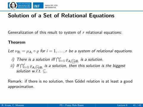
Solution of a Set of Relational Equations

Generalization of this result to system of r relational equations:

Theorem

Let νBi= µAi

◦ for i = 1, . . . , r be a system of relational equations.

i) There is a solution iff⋂r

i=1 Ai©∼Bi

is a solution.

ii) If⋂r

i=1 Ai©∼Bi

is a solution, then this solution is the biggestsolution w.r.t. ⊆.

Remark: if there is no solution, then Gödel relation is at least a goodapproximation.




Solving a System of Relational Equations

Sometimes it is a good choice not to use the largest but one of thesmallest solutions.i.e. the Cartesian product A×B(x , y) = min{µA(x), νB(y)}.

If a solution of νB = µA ◦ exists, then A×B is a solution, too.

Theorem

Let µA ∈ F(X ), νB ∈ F(Y ). Furthermore, let ∈ F(X × Y ) be afuzzy relation which satisfies the relational equation νB = µA ◦ .Then νB = µA ◦ A×B holds.




Solving a System of Relational Equations

Using Cartesian product

µAi= νBi

◦ , 1 ≤ i ≤ r can be reasonably solved with A × B by

= max {Ai ×Bi| 1 ≤ i ≤ r} .

For crisp value x0 ∈ X (represented by 1{x0}):

ν(y) =(

1{x0} ◦ )

(y)

= max1≤i≤r

{

supx∈X

min{1{x0}(x), Ai ×Bi(x , y)}

}

= max1≤i≤r

{min{µAi(x0), νBi

(y)}.}

That is Mamdani-Assilian fuzzy control (to be discussed).




Documents

Fuzzy Systems - Fuzzy Rule Basesfuzzy.cs.ovgu.de/ci/fs/fs_ch06_frb.pdf · Fuzzy Systems Fuzzy Rule Bases Prof. Dr. Rudolf Kruse Christian Moewes {kruse,cmoewes}@iws.cs.uni-magdeburg.de