Embed Size (px)
Citation preview

FUZZY SET-BASED CONTINGENCY ESTIMATING AND MANAGEMENT
Ahmad Salah
A Thesis
in
The Dept. of Building, Civil and Environmental Engineering
Presented in Partial Fulfillment of the Requirements for Master of Applied Science at Concordia University
Montreal, Quebec, Canada
April 2012
© Ahmad Salah

ii
CONCORDIA UNIVERSITY School of Graduate Studies
This is to certify that the thesis prepared
By: Ahmad Salah
Entitled: FUZZY-SET BASED METHODOLOGY FORCONTINGENCY ESTIMATING AND MANAGEMENT
and submitted in partial fulfillment of the requirements for the degree of
Master of Applied Science (Building Engineering)
complies with the regulations of the University and meets the accepted standards with respect to originality and quality.
Signed by the final examining committee:
Chair Dr. A. Bagchi
Supervisor Dr. O. Moselhi
Examiner Dr. A. Hammad External (to program)
Examiner Dr. T. Zayed
Examiner Dr. A. Bagchi
Approved by
Chair of Department or Graduate Program Director
Dean of Faculty
Date

iii
ABSTRACT
FUZZY SET-BASED CONTINGENCY ESTIMATING AND MANAGEMENT
Ahmad Salah, M.A. Sc.
Concordia University, 2012
Contingency estimating and management are critical and necessary functions for
successful delivery of construction projects. Considering such importance, academics and
industry professionals proposed a wide range of methods for risk quantification and
accordingly for contingency estimating. Considerably less work was directed to
contingency management including its depletion to mitigate risk over project durations.
Generally, there are two types of risks; 1) known risks which can be identified, evaluated,
planned and budgeted for and 2) unknown risks which may occurred. These two
categories of risks required a cost and time contingency, even if they weren’t planned for,
in order to mitigate their impact in an orderly manner. In this respect, the importance of
contingency management become critical in view of increasing project complexity and
difficulty of estimating and/or allocating sufficient contingencies to mitigate risks
encountered during project execution. This thesis focuses on the contingency
management from two perspectives; estimating and depletion of contingency over project
durations. A new method is developed using fuzzy sets theory, along with a set of
measures, indices, and ratios to model the uncertainty inherent in this process and
estimate cost contingencies. The uncertainties are expressed in the developed model

iv
using a set of measures and indicators including possibility measure, agreement index,
fussiness measure, ambiguity measure, quality fuzzy number index, fuzziness expected
value ratio, and ambiguity expected value ratio. These measures, indices, and ratios
provide not only the possibility of having adequate contingency but also address issues of
precision and vagueness associated with the uncertainty involved in a generic
computational platform. The thesis, also, presents a comparison between fuzzy existing
methods, Monte Carlo Simulation, PERT, and a proposed direct fuzzy set-based method.
As to depletion, the thesis presents a management procedure focusing on depletion of the
contingency. The developed procedure makes use of policies and procedures followed by
leading construction organizations and owners of major constructed facilities. The
developed method and its computational platform were coded using VB.net
Programming. Two project examples drawn from the literature are analyzed to
demonstrate the use of developed method and to illustrate its capabilities beyond those of
traditional Methods.

v
ACKNOWLEDGEMENTS I would like to express my deepest gratitude and sincere appreciation to my supervisor
Dr. Osama Moselhi for his keen support, guidance, encouragement, and valuable advices
which helped me to sharpen my knowledge and personality during my research.
I would like to extend my deepest thanks to Natural Sciences and Engineering Research
Council of Canada (NSERC), and Dr. Osama Moselhi for the financial support of this
research.
I would like also to thank all Concordia staff, my Concordia friends, and colleagues for
their support not only technically and scientifically but also, socially and psychologically.
I dedicate my thesis to my parents, sisters, and brothers for their support patience and
confidence all the time, especially my youngest sister Waed.
Finally, I would like to express my deep thanks to the person who has always stood by
my side day and night, and provided me continuous understanding and support, my
lovely fiancée Lola Sahmarany.
vi
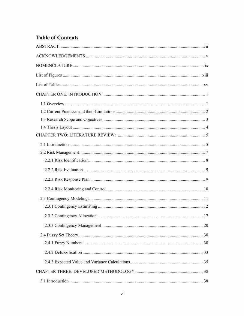
Table of Contents ABSTRACT .................................................................................................................................... ii
ACKNOWLEDGEMENTS ............................................................................................................ v
NOMENCLATURE ....................................................................................................................... ix
List of Figures .............................................................................................................................. xiii
List of Tables ................................................................................................................................. xv
CHAPTER ONE: INTRODUCTION ............................................................................................. 1
1.1 Overview ............................................................................................................................... 1
1.2 Current Practices and their Limitations ................................................................................. 2
1.3 Research Scope and Objectives ............................................................................................. 3
1.4 Thesis Layout ........................................................................................................................ 4
CHAPTER TWO: LITERATURE REVIEW: ............................................................................... 5
2.1 Introduction ........................................................................................................................... 5
2.2 Risk Management .................................................................................................................. 7
2.2.1 Risk Identification .......................................................................................................... 8
2.2.2 Risk Evaluation .............................................................................................................. 9
2.2.3 Risk Response Plan ........................................................................................................ 9
2.2.4 Risk Monitoring and Control ........................................................................................ 10
2.3 Contingency Modeling ........................................................................................................ 11
2.3.1 Contingency Estimating ............................................................................................... 12
2.3.2 Contingency Allocation ................................................................................................ 17
2.3.3 Contingency Management ............................................................................................ 20
2.4 Fuzzy Set Theory ................................................................................................................. 30
2.4.1 Fuzzy Numbers ............................................................................................................. 30
2.4.2 Defuzzification ............................................................................................................. 33
2.4.3 Expected Value and Variance Calculations .................................................................. 35
CHAPTER THREE: DEVELOPED METHODOLOGY ............................................................. 38
3.1 Introduction ......................................................................................................................... 38

vii
3.2 Contingency Estimating ...................................................................................................... 39
3.3 Uncertainty Quantification .................................................................................................. 43
3.3.1 Uncertainty Measures ................................................................................................... 43
3.3.2 Uncertainty Ratios ........................................................................................................ 48
3.3.3 Uncertainty Indices ....................................................................................................... 49
3.4 Contingency Management ................................................................................................... 50
3.4.1. Factors Affecting Contingency Depletion ................................................................... 50
3.4.2 Proposed Depletion Curves .......................................................................................... 53
CHAPTER FOUR: DEVELOPED COMPUTER APPLICATION .............................................. 61
4.1 Introduction ......................................................................................................................... 61
4.2 Characteristics of the Developed Application ..................................................................... 63
4.2.1 Working on a New Project ........................................................................................... 65
4.2.2 Working on Existing Project ........................................................................................ 70
4.2.3 Estimation Module ....................................................................................................... 72
4.2.4 Graphical Module ......................................................................................................... 78
4.2.5 Reporting Module ......................................................................................................... 79
CHAPTER FIVE: APPLICATIONS AND VALIDATION ......................................................... 81
5.1 Introduction ......................................................................................................................... 81
5.2 Contingency and Range Estimating .................................................................................... 82
5.2.1 Case Study 1 ................................................................................................................. 82
5.2.2 Case Study 2 ................................................................................................................. 91
CHAPTER SIX ........................................................................................................................... 100
RESULTS DISCUSSION ........................................................................................................... 100
6.1 Introduction ....................................................................................................................... 100
6.2 Contingency Estimating .................................................................................................... 101
6.3 Contingency Management ................................................................................................. 103
CHAPTER SEVEN: CONCLUSIONS AND RECOMMENDATIONS .................................... 106
7.1 Summary ........................................................................................................................... 106
7.2 Research Contributions ..................................................................................................... 107
viii
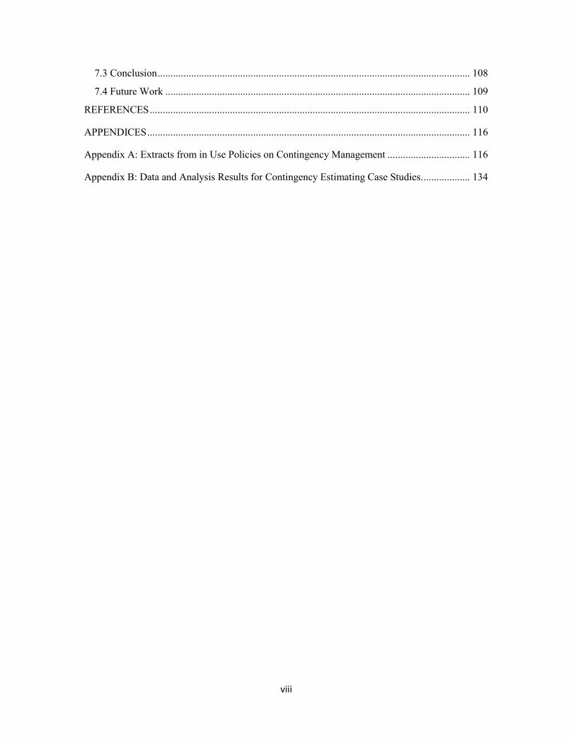
7.3 Conclusion ......................................................................................................................... 108
7.4 Future Work ...................................................................................................................... 109
REFERENCES ............................................................................................................................ 110
APPENDICES ............................................................................................................................. 116
Appendix A: Extracts from in Use Policies on Contingency Management ................................ 116
Appendix B: Data and Analysis Results for Contingency Estimating Case Studies. .................. 134
ix
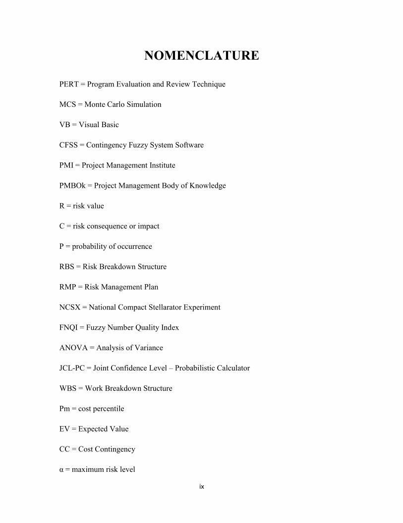
NOMENCLATURE
PERT = Program Evaluation and Review Technique
MCS = Monte Carlo Simulation
VB = Visual Basic
CFSS = Contingency Fuzzy System Software
PMI = Project Management Institute
PMBOk = Project Management Body of Knowledge
R = risk value
C = risk consequence or impact
P = probability of occurrence
RBS = Risk Breakdown Structure
RMP = Risk Management Plan
NCSX = National Compact Stellarator Experiment
FNQI = Fuzzy Number Quality Index
ANOVA = Analysis of Variance
JCL-PC = Joint Confidence Level – Probabilistic Calculator
WBS = Work Breakdown Structure
Pm = cost percentile
EV = Expected Value
CC = Cost Contingency
α = maximum risk level

x
Cov = Co-variance
m = deterministic duration of an activity
D = total duration of an activity
TTA = Total Time Allowance
ATA = Activity Time Allowance
Dpi = Duration Percentile of activity “i”
Tdi = Target Durations of activity “i”
PDF = Probability Distribution Function
fa,, µa = membership function of fuzzy number “a”
COA = Center Of Area
y* = fuzzy number defuzzified value
Var = variance
Ai = fuzzy evaluation of an activity “i”
Aij = jth fuzzy estimation of an activity “i”
Pk = fuzzy evaluation of package “k”
C= fuzzy evaluation of project
F (A) = Fuzziness measure of a fuzzy number “A”
AG (A) = Ambiguity measure of a fuzzy number “A”
P (A) = Possibility measure of a fuzzy number “A”
N (A) = Necessity measure of a fuzzy number “A”
μA (x) = value of membership of a fuzzy number “A” at a given “x”

xi
mλ = combined measure of possibility and necessity measures for given “λ”
FER (A) = Expected Value Fuzziness Ratio of a fuzzy number “A”
AER (A) = Expected Value Ambiguity Ration of a fuzzy number “A”
AI (A, B) = Agreement Index between two fuzzy numbers “A” and “B”
DOE = Department of Energy
CEij = Estimated Contingency for activity “i” over period “dj”
CDij = Depleted Contingency for activity “i” over period “dj”
GUI = Graphical User Interface
DLL= Dynamic Link Library
WF = weight of fuzziness
WAG = Weight of Ambiguity
Err = Error ratio
TC = Total Contingency
NEST = North Edmonton Sanitary Trunk
UHCOC = Urban Highway Construction of California
MPLCC = Mitchell Park Library Community Administration
O.C.P.S. = Orange County Public Schools
FHWA = Federal Highway Association
IEEE = Institute of Electrical and Electronic Engineers
NASA = National Aeronautics and Space
ACi (T) = Actual Contingency for risk Ri during period T

xii
AC (T) = Actual Contingency for all risks during period T
PCi(T) ) = Planned Contingency for risk Ri during period T
PC (T) = Planned Contingency for all risks during period T
RC = Reserve Contingency

xiii
List of Figures
2. 1 Risk Management Procedure: Classic (left) and Modern (right).............................................. 8
2. 2 MPLCC Project Contingency Analysis Report Adopted with Turner(2011) ......................... 26
2. 3 Recommended Contingency Drawdown Curve (Noor et al., 2004; Appendix G) ................. 29
3.1 Contingency Estimating and Management Model ................................................................. 38
3. 2 Contingency Estimation Model ............................................................................................. 43
3. 3 Depletion Curve Types .......................................................................................................... 54
3.4 Custom Contingency Depletion Curve ................................................................................... 55
3. 5 Contingency Management Model ......................................................................................... 58
4. 1 Fuzzy Contingency Estimation Model .................................................................................. 62
4. 2 Contingency Fuzzy System ................................................................................................... 64
4. 3 Creating a New Project .......................................................................................................... 65
4.4 Adding a New Component ..................................................................................................... 66
4.5 Adding a Package ................................................................................................................... 67
4.6 Adding Package Error ............................................................................................................ 67
4.7 Adding a Package ................................................................................................................... 67
4.8 Adding Item Error .................................................................................................................. 67
4.9 Adding a Fuzzy Number ........................................................................................................ 68
4.10 Adding Fuzzy Number Input Error ..................................................................................... 68
4.11 Adding Fuzzy Number Selection Error ................................................................................ 68
4.12 Editing a Component ............................................................................................................ 69
4.13 Saving a Project .................................................................................................................... 70
4.14 Opening an Existing File ...................................................................................................... 71
4.15 Open Project from File Menu ............................................................................................... 72
4.16 Existing Project Loaded as Input .......................................................................................... 72

xiv
4. 17 Adding to Existing Project Interactive Screen .................................................................... 72
4.18 Estimation of Selected Component ...................................................................................... 74
4.19 Fuzziness Weight Input Error ............................................................................................... 75
4.20 Uncertainty Measures Calculations of a Selected Component ............................................. 76
4. 21 Possibility and Necessity Calculation of Selected Component ........................................... 77
4. 22 Degree of Membership Calculations of Selected Component ............................................. 78
4. 23 Graphical Representation of a Selected Component ........................................................... 79
4.24 Project Report ....................................................................................................................... 80
5. 1 Data Input for NEST Project Case Study ............................................................................... 84
5. 2 NEST Case Study Report ....................................................................................................... 86
5.3 Possibility and Agreement Index ............................................................................................. 90
5.4 Itemized Comparison among Proposed Method, PERT and Shaheen Method ........................ 91
5. 5 Data Input of UHCOC Project Case Study ............................................................................. 95
5. 6 UHCOC Case Study Report .................................................................................................... 97
5. 7 Itemized Comparison .............................................................................................................. 98
A- 1 Typical Contingency Drawdown based on Activities ......................................................... 130
A- 2 Periodic Contingency Drawdown Curve: Actual vs. Planned ............................................ 131
A- 3 Contingency Drawdown Report .......................................................................................... 131
A- 4 Risk Weighted Cost Estimates Principles and Practical Application (NASA) ................... 132
A- 5 Contingency Drawdown Curve and Project Milestones ..................................................... 132
A- 6 Estimated Project Cost Post and Pre-Planning of Risks...................................................... 133
A- 7 Project Contingency Drawdown ........................................................................................ 133

xv
List of Tables
2. 1 Projects Budgets (Adopted with City of Jonesboro Doc # 04-046-U) .................................... 27
3.1 Fuzziness and Ambiguity Measures Calculations .................................................................... 47
5. 1 Data of NEST Project Adopted with Shaheen et al. (2007) .................................................... 82
5. 2 Comparison of Results ............................................................................................................ 86
5.3 the Proposed Method Uncertainty Modeling Associated with NEST Project .......................... 88
5. 4 UHCOC Positive Risks Data Input ......................................................................................... 92
5. 5 UHCOC Negative Risks Data Input ........................................................................................ 93
5. 6 Comparison of Results (Case 2) .............................................................................................. 97
1
CHAPTER ONE
INTRODUCTION
1.1 Overview
Construction industries have been developing and growing in many ways, and the
number and scale of construction projects has been increasing in tandem. A risk
management plan plays an ever-increasingly important role in any project’s success. An
adequate risk management plan makes it possible for a project to deal with risks
(threats/opportunities); to make appropriate and timely responses which minimize the
losses or increase the benefits associated with those risks.
Risk management has therefore been attractive area to researchers, who focus on risk
identification, evaluation, response, monitoring, and control. The risks associated with a
project require contingency resources to be mitigated. Several contingency estimation
and contingency allocation methods can be found in the literature, based on experience
(percentage of the total project cost), PERT, Monte Carlo simulation, and other methods.
Compared to the number of studies directed towards contingency estimation and
allocation subjects, it was noted that considerably less work has been focused on
contingency management, including its depletion over project durations.
Consequently, this research focuses on contingency, from two perspectives: 1) its
estimation, using the fuzzy set theory, and 2) its management, using practitioners’
methodologies.

2
1.2 Current Practices and their Limitations
Several methods have been developed to estimate, allocate and manage contingency. The
majority of these methods are based on two classic approaches; deterministic and
probabilistic. In addition, researchers have recently introduced the use of fuzzy set
theory. Both the deterministic and probabilistic approaches still have several drawbacks
and limiting assumptions, such as: the subjectivity of estimators, the availability of
historical data, and a probability distribution’s function shape (i.e. normal, beta,
logarithmic or exponential).
In addition, the contingency management procedures and guidelines followed by
construction industries have several differences and discrepancies. The meaning of
contingency management differs from one organization to another. Each organization
therefore generates its own contingency management methodology, enveloped by its own
experience in similar projects and its policies. The different policies and their variances
have made it impossible to document or implement a general methodology for
contingency management or depletion per current practice. This situation clearly shows
the need to create a unified and systematic methodology for contingency management.
Moreover, project managers use different strategies to deal with contingency depletion,
strategies that are widely spread between optimistic, also called aggressive strategy, and
pessimistic, or passive strategy. Contingency depletion is affected by several factors,
many of which are not usually considered in a contingency management plan.

3
1.3 Research Scope and Objectives
This research addresses contingency management with a focus on its estimation and
depletion over the project durations. This objective was set to be achieved by first
studying the risk management environment and risk quantification methods. Current
industries practices in contingency estimating and in contingency depletion were
analyzed, and a new methodology utilizing linguistic expressions, normally used by
practitioners, was developed to model the uncertainty associated with the project’s
contingency. The developed method for contingency depletion makes use of the current
practices of leading owners and managers of constructed facilities. The sub-objectives of
this research are:
1. To study and analyze the advantages and limitations of contingency estimating
methods in literature.
2. To study and analyze contingency management and depletion current practice
based on: literature examples, project under-construction reports, construction
companies’ procedures, and government policies.
3. To study and analyze the factors affecting contingency management and propose
a procedure to assist companies in selecting appropriate contingency depletion
curves based on these factors.
4. To develop a contingency estimating methodology based on fuzzy set theory in
order to overcome the aforementioned limitations.
5. To develop a new methodology for contingency management and depletion
6. To design and code user- friendly computer software to support the application of
the proposed contingency estimating methodology using VB.net.

4
1.4 Thesis Layout
Chapter 2 presents a literature review on risk management, contingency estimating,
contingency management, fuzzy set theory, existing methods, depletion curves, current
practices and policies. The proposed contingency estimation methodology based on fuzzy
set theory is presented in chapter 3, including the factors that affect the different types of
depletion curves,. The chapter also describes and shows the development of a new
methodology for contingency management based on depletion curves, introducing a
procedure for depletion curve selection based on an IF-AND-THEN approach. Chapter 4
shows the development of Contingency Fuzzy System Software (CFSS) using VB.net,
including a detailed description of its capabilities, characteristics, and a detailed user-
guide. The contingency estimating methodology and the CFSS results are validated by
their application on two case studies extracted from the literature, as described in chapter
5 The contingency management methodology and depletion curve selection procedure is
also validated in chapter 5, based on two case studies drawn from current practice.
Chapter 6 presents a discussion of the proposed methodologies of contingency estimating
and management based on case study results and in comparison to current methods and
procedures. Chapter 7 presents the thesis conclusions, contributions and
recommendations for future research.

5
CHAPTER TWO
LITERATURE REVIEW
2.1 Introduction
Several methods commonly used to estimate, allocate and manage construction project
contingency are available in the literature. This chapter focuses on the most popular
methods, highlighting their respective advantages, limitations, and disadvantages, as well
as, their application domains.
Researchers have mainly concentrated their efforts on contingency estimating, even more
so than on allocation, while considerably less work has been directed toward contingency
management. Contingency management is, however very important to successfully
manage contingency resources over a project’s duration, made possible by implementing
one of the depletion methods. The selection of a contingency depletion curve for a
specific project depends on various factors; factors which are prioritized differently for
each company. During project execution, the contingency manager asked two questions:
1- how to manage this contingency? , 2- how to deplete it?
The exhausting of contingency prior to project completion is considered a serious and
grave condition (Diekmann et al., 1988). At the same time, excess contingency at project
completion is not necessarily a sign of risk management plan success or of the
effectiveness of contingency depletion as many of project managers believe (Ford, 2002).
6
The contingency managers (i.e. project manager) use common practice to manage
contingency based on their experience and judgement (Ford, 2002). The lack of
contingency management standards, documented methods and tools in the literature has
thus led us to direct our research to contingency methods, tools and practice.
Contingency amounts are used to mitigate the risks associated with a project over its life
cycle. The literature includes numerous definitions; the risk definition given by Project
Management Institute (PMI) in the Project Management Body Of Knowledge (PMBOK)
is “risk is an uncertain event or condition that, if it occurs, has a positive or negative
effect on project’s objectives” (PMI, 2003).
Raymond Madachy (2002) asserts that “The risk is the possibility of an undesirable
outcome: excess budget, schedule overrun, and deliver unsuitable product” (Raymond
Madachy, 2002).
The risk value depends on the probability of occurrence “P” and the corresponding
consequence or impact “C” (Zhou, ASCE and Zhang, 2010).
R = P × C (2.1)
Where,
P is the probability of occurrence of a risky event during the project’s life cycle, and C is
the consequence of a risky event.
The events list below should NOT be considered as risks (White, 2006):
Event 1: if the event will never occur under any circumstances (P=0 R=0)
7
Event 2: if the event is certain and it will occur in any case (P=1 R = C)
Event 3: if the event does not have any impact if does or does not occur(C=0 R=0)
Any event where 0<P<1 and C≠0 will be considered, evaluated, planned, mitigated and
controlled for over the project duration. Risks with a positive value of C are called
opportunities and those with negative impacts (negative C value) are known as threats. In
the thesis we deal with risk regardless of its status as an opportunity or a threat.
There are two types of risk associated with projects:
- Known risks, also called “predictable risks”: these risks can be identified, evaluated,
planned for, monitored and controlled; and
- Unknown risks also called “un-predictable risks” or “unknowable unknowns”: these
risks cannot be identified, planned, monitored or controlled for since they become known
when they occur.
2.2 Risk Management
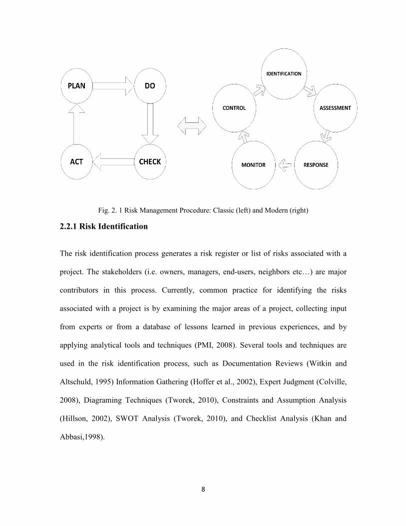
Risk management is the current elaboration or new implementation of the classic project
management procedure “plan -> do -> check -> act”; the current practice is to develop a
plan for risk management by carrying out risk identification, risk evaluation, risk
response plan, risk monitoring and risk control (KWAN and LEUNG, 2010). Stackpole
(2010) summarized risk management; dividing it into three major components or outputs:
a risk breakdown structure (RBS), a risk template, and a probability and impact matrix
(Stackpole, 2010). The traditional project management procedure can be re-formed into a
modern risk management procedure as shown in (Error! Reference source not found.).
8
Fig. 2. 1 Risk Management Procedure: Classic (left) and Modern (right)
2.2.1 Risk Identification
The risk identification process generates a risk register or list of risks associated with a
project. The stakeholders (i.e. owners, managers, end-users, neighbors etc…) are major
contributors in this process. Currently, common practice for identifying the risks
associated with a project is by examining the major areas of a project, collecting input
from experts or from a database of lessons learned in previous experiences, and by
applying analytical tools and techniques (PMI, 2008). Several tools and techniques are
used in the risk identification process, such as Documentation Reviews (Witkin and
Altschuld, 1995) Information Gathering (Hoffer et al., 2002), Expert Judgment (Colville,
2008), Diagraming Techniques (Tworek, 2010), Constraints and Assumption Analysis
(Hillson, 2002), SWOT Analysis (Tworek, 2010), and Checklist Analysis (Khan and
Abbasi,1998).

9
2.2.2 Risk Evaluation
The risk evaluation process includes the analysis and evaluation of risks, both
quantitatively and qualitatively. This process is considered as a screening process for the
risk register since risks with low risk value (low probability and low impact) that fall
below the range of risk tolerance of a project will be disregarded.
Several methods can be used in qualitative risk evaluation as well as in quantitative
evaluation. The most commonly used methods or techniques are: risk matrix (Abdel
GAWAD et al., 2008), Monte Carlo simulation (Seppala, 2008), decision trees
(Thompson and Perry, 1992) and regression analysis. The output of a risk evaluation
process will be input of its corresponding risk response plan.
2.2.3 Risk Response Plan
A risk response plan is a list of risk mitigation actions/options that can be taken to
minimize the effects of a threat (negative impact) or maximize the benefits of an
opportunity (positive effect). The threat responses are: avoid, transfer, mitigate and
accept, while the opportunity responses are: exploit, share, enhance and accept
(Stackpole, 2010).
Risk management plan (RMP) or risk response plan (RRP) incorporate responses to all
risks associated with activities, packages, or projects listed in a risk register, including
those with a low impact (acceptable risk based on a project’s risk tolerance). The risk
mitigation, by applying on of the action listed in the risk response plan, will deplete

10
project resources such as: time and cost. These resources are known as “project
contingencies” in risk management.
There are several commonly used methods and techniques to formulate risk response plan
such as: 1) a planning decision flowchart, 2) problem solving planning, 3) an action item
list, and 4) risk information sheets. Since the recommended responses are not “solutions”,
they should be monitored and controlled throughout the life cycle of the project.
2.2.4 Risk Monitoring and Control
Risk monitoring is an on-going process throughout the project’s life cycle (PMI, 2008).
This valuable process is necessary to evaluate the performance and effectiveness of a risk
response plan. The methods used to monitor risks over a project’s duration include, but
not limited to: 1) bar graphs, 2) time graphs, 3) risk information sheets, 4) time
correlation charts.
Any response failure that occurs during the monitoring process will trigger the control
process. The risk control process will also be triggered when decision makers, based on
available data from monitoring process, decide to re-assess risk or to update the risk
responses in order to increase the manageability and controllability of risk occurrence and
impact (Kwan and Leung, 2010). Some of the commonly used methods in risk control
are: closing risk, cause and effect analysis, cost / benefits analysis, and problem solving
analysis. The output of the risk control process is used to evaluate the risk management
plan’s performance.
11
2.3 Contingency Modeling
Contingency has several definitions in the literature. The Project Management Institute
defines contingency as “The amount of funds, budget or time needed above the estimate
to reduce the risk of overruns of project objectives to a level acceptable to the
organization” (PMI, 2004). The American Association of Civil Engineers (AACE)
defines contingency as “An amount added to an estimate to allow for items, conditions,
or events for which the state, occurrence, or effect is uncertain and that experience shows
will likely result, in aggregate, in additional costs” (AACE, 2007).
Contingency has an important role in risk management and project success because it
increases the ability to mitigate risks associated with project cost overrun and/or project
delay. Therefore, it is important to estimate project contingency properly so that it can
play its designate role. In addition, contingency should be accurately estimated,
reasonably allocated, and wisely managed over project durations (Barraza et al. 2007).
Without project contingency, a risk responses plan is useless, risk management has little
or no function, the probability of a project suffering from cost overrun is high, and the
project may reach an endpoint. For example, the National Compact Stellarator
Experiment (NCSX) project had started in 2004 with a baseline contingency (cost =28%,
time =10% = 5 months) to support its risk management plan. During 2004-2007, a reform
risk management was implemented in order to reduce additional cost and delays. Even
though, a reformed of risk management plan enhances a project’s performance, in this
project, unfortunately, its effects were not sufficient to allow it to continue. As a result,
NCSX’s project was cancelled in 2008 because of the estimated cost increases at

12
completion (>70%) and because the forecasted completion date was pushed back by 4
years (Neilson et al., 2010). This example reflects the importance of contingency
estimating, allocation and management for any project.
A variety of different approaches can be found for estimating, allocating, and managing
contingency, such as the deterministic, probabilistic, and fuzzy approaches. It is
important to categorize the existing methods into three main functional categories:
estimating, allocation, and management. Furthermore, these categories could be sub-
categorized based on the contingency being studied: cost or time.
2.3.1 Contingency Estimating
Contingency estimating has been the main focus of several studied and a number of
researchers, and can be performed utilizing an unlimited number of methods. These can
be clustered in three main groups: deterministic methods, probabilistic methods, and
fuzzy set-based methods. Contingency estimating is important for:
• Risk management plan applicability: if there are not enough contingency funds,
the risk management plan in place is useless (Ruskin, 1981).
• Project success: if contingency is estimated accurately, there is a low probability
of project cost overrun and delay (Baccarini, 2006).
Deterministic methods use point estimates which represent input parameters (i.e. cost,
contingency percentages etc...). These estimates are usually based on average value,
maximum value, expert judgement, and experience, and can result an underestimated or
overestimated values (McGrew and Bilotta, 2000). Deterministic methods have a
13
relatively low degree of accuracy compared to probabilistic methods, but they are very
useful when historical data is not available. Based on the details required for contingency
estimating, two types of deterministic methods can be identified: overall estimated value
and itemized evaluation method (Moselhi, 1997).
Probabilistic methods use, the contingency value and the likelihood that the contingency
needs will not exceed this estimated value. If historical data is available, these methods
can yield estimates that are more accurate than those of deterministic methods. The
degree of a probabilistic method’s accuracy is related to the available data volume. For
example: when minimum data is available only low accuracy can be achieved.. This
approach assumes that contingency items can be represented by a specific probability
distribution function (Barraza and Bueno, 2007). Probabilistic methods may be clustered
in two categories based on the estimator’s assumptions: independent items, and correlated
items (Sonmez et al., 2007). According to Moselhi (1997), each category can be applied
with or without simulation (i.e. Monte Carlo Simulation).
Fuzzy set-based methods use experts’ linguistic assessment of the risks involved. The
fuzzy number may be represented by two ranges (i.e. the maximum range and the most
probable range) which increase the accuracy of an expert’s estimate (Paek et al., 2003). A
fuzzy approach can be applied when contingency items follow any type of distribution
(i.e. crisp, uniform, triangular, trapezoidal) and when there is no historical data available.
Several researchers focus on cost contingency estimating. Paek et al. (1993) proposed a
method for pricing project risk and calculating contingency needed to mitigate risks
associated with a project. The proposed method uses fuzzy set theory and the ranking

14
method proposed by Chen (1985) to calculate total project contingency (Paek et al, 1993;
Chen, 1985). The advantages of this method are: 1) the use of fuzzy set theory, 2) the
accommodation of expert subjectivity with a systematic estimation procedure. Its
disadvantages are: 1) a dependency on project type, 2) its non-user-friendly algorithm
application (there has been software developed to incorporate most of this algorithm, but
validation of results is still not an easy task).
Osama Moselhi (1997) claims that the methods and techniques used for contingency
estimation are primarily traditional algorithm methods and they range from crystal-ball
(gut-feel method) to Monte Carlo Simulation (probabilistic method). Moselhi proposed a
direct probabilistic method that considers the correlation that may exist between project
cost items. The advantages of this method are: 1) simplicity, 2) it takes less time than
other methods (i.e. Monte Carlo Simulation), and 3) it provides an acceptable
contingency estimating range. The disadvantages are that it assumes that cost items are
normally distributed, as well as the availability of historical data (Moselhi, 1997).
Touran (2003) proposes a method to estimate contingency for construction projects based
on change orders which may arise throughout a project’s duration. Touran’s method
depends on several variables, such as: 1) estimated rate of change (α), 2) project duration
(T), 3) average cost per change order (µc), and 4) the variation’s coefficient of change
order’s cost (fc). The advantages of this method are: 1) simplicity, 2) less-parametric. The
disadvantages or limitations are its assumption that change orders are Poisson distributed,
and its application is limited to construction projects and only in the early stages (i.e.
budgeting and planning) (Touran, 2003).
15
Cost contingency estimating attracted Barraza and Bueno’s (2007) attention and led them
to propose a method based on Monte Carlo simulation. They propose a total project
contingency estimating method based on normal distribution with an assumed project
probability of being under-run (i.e. 80%). The proposed method has a simple application
and uses known parameters, but it assumes that activity costs are independent and
normally distributed, which is not always the case (Barraza and Bueno , 2007).
Shaheen, Fayek and Aburizk (2007) propose a method for estimating project cost range
using fuzzy set theory. The authors proposed a procedure using the Delphi method for
experts’ estimates, based on the deviation between the individual estimated value and the
average estimated value of each cost item. The fuzziness measure, ambiguity measure
and FNQI (fuzzy number quality index) can then be calculated. Their method calculates
cost range, represented by a fuzzy number, and its expected value is most likely value of
a project. The advantages of this approach are that it is faster and less-time consuming
(only one iteration is needed). The disadvantages of this method are: 1) the proposed
estimation process may take a long time to unify experts’ input using Delphi method
(iterate until two consecutive inputs average are quite similar); 2) formulas used to
calculate the expected value are complicated and difficult to be verified, especially for
trapezoidal fuzzy number (Shaheen et al., 2007) and 3) the selected measures (fuzziness,
ambiguity, and FNQI) are not adequate to evaluate the quality of the results.
Given the current relative lack of research in estimating cost contingency, Thal, Cook,
and White (2010) propose a model that stars with the identification of the factors
impacting cost contingency based on ANalysis Of VAriance (ANOVA) procedure and a
regression analysis. The model generates a contingency estimating formula using
16
combination of the significant factors thereby identified (which have significant impact
on increasing cost contingency). The advantages of this model are that it: 1) reduces the
contingency fund shortage; 2) tailors the contingency based on project-specific risks; and
3) generates reliable results in the earlier project stages (budgeting, planning, and contract
award). This model has several limitations and disadvantages, such as: 1) the use of
regression analysis, which depends upon a relevant data range; 2) assuming that the same
factors which affected contingency in the past will do the same thing in the future; 3) it
only deals with over-run; 4) it uses information that is available only up to contract
awarding; and 5) it is limited to air-force projects (Thal et al., 2010)
Another method for cost contingency estimating was recently proposed by Idrus,
Nuruddin and Rohman in 2010. Their proposed method uses risk analysis and a fuzzy
expert system and can be described by seven stages: development of a conceptual model
for cost contingency, determination of risk factors, development of a fuzzy expert system,
model testing, tuning, and validation. The advantages of this proposed method are that it
is flexible, rational, and it uses fuzzy expert system. This method’s limitations are: 1) it is
time-consuming; and 2) it relies on the availability of historical data for tuning purposes
(Idrus et al., 2010).
Touran and Zhang (2011) propose a new method for contingency estimating based on the
project completion percentage. Their proposed method is a modified version of the
NASA JCL-PC (Joint Confidence Level – Probabilistic Calculator) method. The analysis
gives results at 70%, 75% and 80% confidence levels. This method’s advantages are: 1)
the simplicity of its application, and 2) its ability to detect the possibility of a project’s
cost overrun at any milestone. The disadvantages are: 1) it assumes the availability of
17
historical data for similar projects; and 2) its application is limited to infrastructure
projects (Touran and Zhang, 2011).
Other methods can be found in literature, such as: the crystal ball method, which
considers a project cost’s percentage as contingency (e.g. 10%), and which is arbitrary
and difficult to defend (Baccarini, 2006), the Monte Carlo Simulation (Vose, 1996), the
Artificial Neural Network method (Chen and Hartman, 2000), and the linear regression
(Williams, 2003).
Most researchers in the contingency field have focused their work on cost contingency
based on the assumption that “time is money”; considering that any required time
contingency can be evaluated by its cost. Despite this overriding perspective, some
researchers have focused on time contingency estimation as a separate subject using
probabilistic methods (Barraza, 2011) and deterministic methods (Mohamed et al. 2009).
2.3.2 Contingency Allocation
The same approaches of contingency estimating, especially the deterministic and
probabilistic approaches, are applicable to contingency allocation, except for the fuzzy
approach, which is rarely used for contingency allocation. A project’s contingency
estimating cannot answer the questions usually asked by project managers: 1) Where (or
when) should these contingencies be used?; and 2) How much contingency is allocated to
each activity? Researchers have therefore extended contingency allocation from the
project level (global contingency estimation) to the activity level (local contingency
estimation) and can now provide a fair distribution between project activities based on
their risk level (Barraza 2011).

18
Barraza (2011) proposed a heuristic approach using Monte Carlo Simulation (MCS) to
assign project cost contingency to activities (depending upon the work breakdown
structure details). The proposed method assumes that each activity has a probability
distribution, an expected value (EV) and a cost percentile (Pm) or the budgeted cost
calculated at the maximum risk level (α).
CCi = Pmi − EVi (2.2)
The maximum risk level is calculated where the cost of a project is equal to the budgeted
cost. The main advantages of this method are that it increases the ability to control
contingency, and it gives the project manager a fair allocation methodology for
distributing the contingency fund among project activities based on Work Breakdown
Structure (WBS). The main disadvantage of this method is that it assumes that all
activities have same level of risk (needs contingency) which is not always the case
(Barrazaand Bueno, 2007).
Williams (1999) focused on time contingency allocation in the activity duration network
by introducing a new measurement called the “Curciality”. The proposed method uses the
PERT method with no uncertainty to calculate the deterministic length of each activity
(m), its mean value, and covariance (Cov) calculated from simulation results. Then, by
using a trial and error method, the maximum risk level (α) could be calculated in order to
allocate the contingency of each activity (α × Cov). The total duration of the activity is
represented as:
D = m + α Cov (2.3)

19
This method distinguishes between the contingency and float allowance of each activity
and identifies the most crucial activity (the one actually causing the risk). The
disadvantages of this method are that it: 1) eliminates the uncertainty of activities’
durations, 2) time consuming (using trial and error method), and 3) is difficult to use in
complex projects (Williams, 1999).
Consequently, Barraza (2011) has devoted considerable attention to the allocation of time
contingency, since it is as important as cost allocation. He proposed a new method to
allocate the corresponding time contingency of each activity. In other words, he
distributes total time contingency of a project among its activities, represented as:
TTA = ∑ ATA𝑖𝑖=𝑛𝑖=1 (2.4)
Where, activity time allowance (ATAi) is calculated by the difference of maximum
duration percentile (Dpi) and the target duration (Tdi). The advantage of this proposed
method is the equitable distribution of time contingency among project activities. But
unfortunately, as with cost contingency allocation, it assumes that all activities have the
same risk level and that the probability distribution function (PDF) shape of each activity
is known (Barraza, 2011).
Researchers use other methods for time contingency allocation based on conventional
lump-sum multiplying the activity duration by same percentage of total project time
contingency (e.g. 10%) also called crystal ball method (Moselhi, 1997; Baccarini 2006),
by using probabilistic itemized allocation (called also Pareto’s Law), PERT, Monte Carlo
Simulation (Kwak and Ingall, 2007), Artificial Neural Network (Chen and Hartman,
2000), and by using fuzzy set theory (Jin and Doloi, 2009).

20
The procedures followed by practitioners for contingency allocation are slightly different.
For example: the States of Jersey has a policy of contingency allocation based on three
types of expenditures (Appendix A):
• Permanent and Non-Repayable: expenditures due to a change in circumstances or
service requirements;
• Short Term and Repayable: Expenditures arising from departmental opportunities
for “Invest-to-Save” initiatives; and
• Variation in Expenditure that have a “Net-Nil” impact: expenditures that may
require variation between expenditure headings with no overall impact on the
contingency balance.
Based on these three types a request for allocation of expenditures should be sent to
the approval authority. The approval request includes: 1) the description, 2) the
justification, 3) the recommendations, and 4) the amount. If the request is not
approved, the allocation request will be returned to the originating department.
Otherwise, the request is approved, distributed, and an equal amount of contingency
is allocated to mitigate the risk(s) interpreted in this request (States of Jersey, 2012).
2.3.3 Contingency Management
Compared to contingency estimating and allocation, researchers have directed
considerably less work towards contingency management research. Several studies began
by targeting contingency management but have unfortunately being focused on either
contingency estimating or allocation. For example, Yeo (1990) paid a considerable work

21
on contingency research and proposed a method to estimate, allocate, and monitor
contingency but which unfortunately does not address how to manage it.
Ford (2002) found that contingency management practices are not as well-defined or
organized as other managerial activities. He therefore made an effective effort toward
contingency management by proposing a model based on project manager practices. The
model represents the common practices of a contingency manager (i.e. Project Managers)
from different companies and formulates the gut-feel management procedure followed by
the project managers interviewed. The proposed model contains four accounts:
emergency (or cost), schedule, improvement (quality), and excess. All the accounts start
with 25% of the project contingency. Two types of transfer are then possible among these
accounts: 1) Re-allocate to the left: transfer contingency from the current account to the
account on left, and 2) Re-allocate to the right: transfer contingency from the current
account to the account on right. Each account has two inputs: 1) to receive left re-
allocations, and 2) to receive right re-allocations, and three outputs: 1) to mitigate risk, 2)
to re-allocation “to the right”, 3) to re-allocation “to the left”. The reallocation between
different accounts is well implemented by a series of 30 formulas (Ford, 2002).
Ford’s model introduces two type of management strategy: passive and aggressive
(active). The passive and active strategies have five characteristics: 1) evolution of the
contingency reallocation speed, 2) evolution of the schedule perception, 3) speed
adjustment, 4) evolution of the willingness to use contingency to control a schedule, and
5) the escrow fraction used for improvement. The application of a strategy depends on
the management skills of project manager, who is usually encouraged: 1) not to spend
contingency too early in order to assure timely project completion, or 2) to spend at an

22
early stage when it can add value to the project (quality), or 3) to have an excess of
project contingency at completion. The author found that a passive strategy performs
better in emergency situations and for better schedule control, while an aggressive
strategy performs better at absorbing changes in project conditions (Ford, 2002). The
advantages of this model are that it: 1) gives current practice a formal procedure, 2)
generalizes the decision making processes used in contingency management, and 3)
establishes an interested contribution in contingency management. The disadvantages of
this model include: 1) it is a subjective method because it depends on a project manager
skills and his/her preferred contingency management strategy (aggressive or passive), 2)
it only deals with cost contingency and omits the time contingency (i.e. time is money),
and 3) it depends on a project manager having either an optimistic (aggressive strategy)
or pessimistic (passive strategy) personality.
Barraza (2007) proposes a method to manage cost contingency using a simple heuristic
method and Monte Carlo simulation. The proposed method controls project contingency
by comparing the activities’ allocated contingency versus the contingency used. The
individual comparison evaluates the contingency performance (status) at a cost item level
and the cumulative contingency evaluates the contingency performance (status) at the
project level. Based on the required contingency the activity’s (or project’s) status varies
between A (Positive), B (negative but less than the allocated contingency) and C
(negative and greater than the allocated contingency). This method provides the ability to
monitor cost contingency over the project durations, it allows more efficient management
and thus can process corrective action implementation, and it allows contingency
performance to be monitored at both the activity and project levels. The disadvantages of
23
this method are: 1) while easy to use in simple projects, it is not at all easy in complex
projects, 2) it gives the ability to monitor without the capability to control or manage, and
3) it assumed that all of the activities’ durations are normally distributed and that they
have the same risk level (Barraza and Bueno, 2007).
Barraza (2011) proposes a new method for time contingency management using the
allocation of time contingency at the activity level. In this method, the project manager is
requested to control the activity’s targeted contingency and to manage it so that it is equal
to or less than the activity’s allocated contingency. The advantages of Barraza’s method
are: 1) its simplicity; and 2) the easy implementation using commercial software like
Excel and Crystal Ball. The disadvantages of this method are: 1) it is a subjective
method, and 2) it depends on the project manager’s skills and strategy. In addition, it does
not take into account the unknown risks and the risks at project level (Barraza 2011).
The literature does not reflect the actual practices of contingency management.
Therefore, this research focuses on the practical application of contingency management
extracted from several sources in the construction industry including: 1) government
projects (i.e. Department of Transportation, Energy, and Defense), 2) private companies
procedures (i.e. OCPS), and 3) municipalities policies (i.e. States of Jersey and City of
Palo Alto). These practices follow different methodologies which consider several
assumptions, and reference important factors based on the organization’s subjectivity in
decision making. The contingency is managed by studying each risk separately and
controlling it based on the contingency required for mitigation. If the required
contingency is higher than the planned contingency, an approval of additional
contingency use would need to be requested. The approval procedure depends on the

24
organization’s policies and experience (Appendix A). Each organization follows its own
practice in contingency management. Some examples of the practices considered in this
research are:
• The policy of contingency management followed by Naval Special Warfare
Command indicates an approval procedure for using contingency. The procedure
includes an approval hierarchy based on responsibilities and delegations, ruled by
the following criterion (Naval Special Warfare Command, 2008):
o If the additional contingency fund required is less than or equal to $25,000
it could be approved by the NSWC facility engineer. Otherwise, it should
be approved by the NSWC program manager.
• A project’s can be estimated based on a fixed percentage of project cost (i.e. 5%) and
this percentage could be increased based on experience, project type, lessons learned
and company experience in similar projects (Appendix A). A study on the Trail
Projects awarded by the City of San Jose between 2002-2009 shows that 40% (6 of
15) of project with contingency less than 5% suffered from cost overrun, and same
situation occurred for projects with a contingency of 5 to 10%. Only 20% of the
projects with contingencies greater than 10% suffered from cost overrun. Therefore,
San Jose decided to increase the planned contingency for future Trail Projects from
5% to 10% (City of San Jose, 2009).
• A procedure which includes a request to use the contingency that depends upon a
project and contract types. It considers that each contract/project type could have
different types of request forms (i.e. GMP). Requests should include the following
information: risk description, risk total cost or amount required, justification,

25
responsible or risk owner, amount balance, and the reason(s) for approval or
disapproval (Appendix A).
• A procedure that can be generated by mixing several procedures, including: 1)
approval procedures, 2) delegations of responsibility between different management
levels, and 3) contingency limitation to 5%, 10% or an amount of $200,000
(Appendix A). The Federal Highway Association (FHWA) and the department of
transportation of Canada consider that contingency depletion should be based on: 1)
the amount, 2) the justification, 3) the approval authority, and 4) the funding sources.
Several rules are involved in this process, such as:
o Occurred risk has an allocated contingency or not;
o Funding source is federal or non-federal; and
o Contingency depletion requested is less or greater than specified amount
(i.e. $200,000).
• Some companies, based on their experience, build a typical drawdown plan for
contingency management and depletion (Appendix A). According to the “Managing
Major Projects” (MMP) website, the drawdown procedure should follow a specific
depletion plan over project durations based on the company’s experience in similar
projects. MMP considers that the contingency depletion of each activity is a weighted
percentage of total contingency (Appendix A).
Further to the contingency management literature reviewed above, two case studies are
examined in depth and later utilized in the developed contingency management method.
Each is described below.

26
The first case study is “Mitchell Park Library Community Center” project for City of
Palo Alto – California – USA was awarded to TURNER Construction in 2011. The
projected cost is $ 41 M and the budgeted cost is $49 M. The project started with a
contingency of 10% ($2.44 M) of the $ 24.4 M total construction cost. In September
2011, the project’s contingency was increased by an additional 15% ($3.65 M). The
reason of this increase is the unforeseen risks (i.e. existence of PG & E High Pressure
Gas Line) and the unknown risks: 1) withdraw of steel structure sub-contractor, and 2)
the exterior cladding was changed in order to meet the performance required in the
project’s specification. In this project, Linear Depletion Curve was selected by Turner as
the contingency depletion baseline for post and pre-extension of contingency as shown in
Error! Reference source not found..
Fig. 2.2 MPLCC Project Contingency Analysis Report Adopted with Turner(2011)
27
However, the actual contingency depletion curve could have a different and unpredictable
shape based on the risks encountered (unknowns, unforeseen, and under-evaluated) and
the approved “change orders”. The dashed line represents actual approved change orders
on monthly basis while the shaded area represents the area bounded by minimum
projected change orders (18%) and maximum projected change orders (23%).
The contingency depletion baseline, shown in Error! Reference source not found. is a
linear curve starting from 0% at project start-up to 10% at project completion. But after
contingency amendment, Turner assumes that the project contingency will be depleted
linearly. This indicates the linear depletion curve used by Turner in the current practice. It
should be noted that Turner continues to use a linear contingency depletion curve (i.e.
using linear contingency depletion curve before and after the extension of the project’s
contingency).
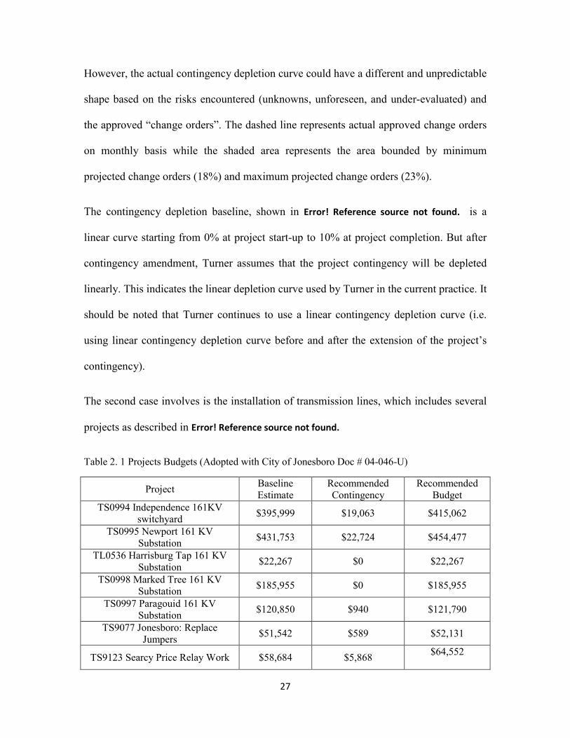
The second case involves is the installation of transmission lines, which includes several
projects as described in Error! Reference source not found.
Table 2. 1 Projects Budgets (Adopted with City of Jonesboro Doc # 04-046-U)
Project Baseline Estimate
Recommended Contingency
Recommended Budget
TS0994 Independence 161KV switchyard $395,999 $19,063 $415,062
TS0995 Newport 161 KV Substation $431,753 $22,724 $454,477
TL0536 Harrisburg Tap 161 KV Substation $22,267 $0 $22,267
TS0998 Marked Tree 161 KV Substation $185,955 $0 $185,955
TS0997 Paragouid 161 KV Substation $120,850 $940 $121,790
TS9077 Jonesboro: Replace Jumpers $51,542 $589 $52,131
TS9123 Searcy Price Relay Work $58,684 $5,868 $64,552

28
TL0536 Harrisburg – Marked Tree Tline $796,110 $47,480 $843,590
TL0537 Paragouild- AECC Paragouild S Tline $2,341,017 $26,440 $2,367,457
TL0538 Jonesboro – Jonesboro SPA Tline $528,827 $29,982 $558,809
TL9006 ISES – Newport New Tline $4,354,978 $476,615 $4,831,593
Total $9,287,982 $629,701 $9,917,683
The recommended contingency depletion curve shown in Error! Reference source not
found. could be considered as S-curve. The drawdown curve is representative of all
projects combined which could be supported by individual project contingency depletion
curves to increase ability to control contingency totally and individually as stated the
agreement (City Of Jonesboro, 2004).

29
Fig. 2. 3Recommended Contingency Drawdown Curve (Noor et al., 2004; Appendix G)
The above example shows that the contingency management’s proposed method could be
combined to multiple projects and individual project which expands the applicability
domain of the proposed method.
Moreover, the example of managing major projects (MMP) presented in the Appendix A
describes an actual drawdown contingency curve and a planned depletion curve which
prove the importance of the comparison between the actual and planned drawdown
contingency curves. This comparison increases the project manager’s ability to monitor
and control the project contingency depletion. In addition, another perspective of
30
contingency depletion was introduced which uses the percentage of total contingency for
each activity based on risks associated with it (MMP). Finally, a monitoring method was
introduced based on depleted and balance as shown in Fig. A- 3.
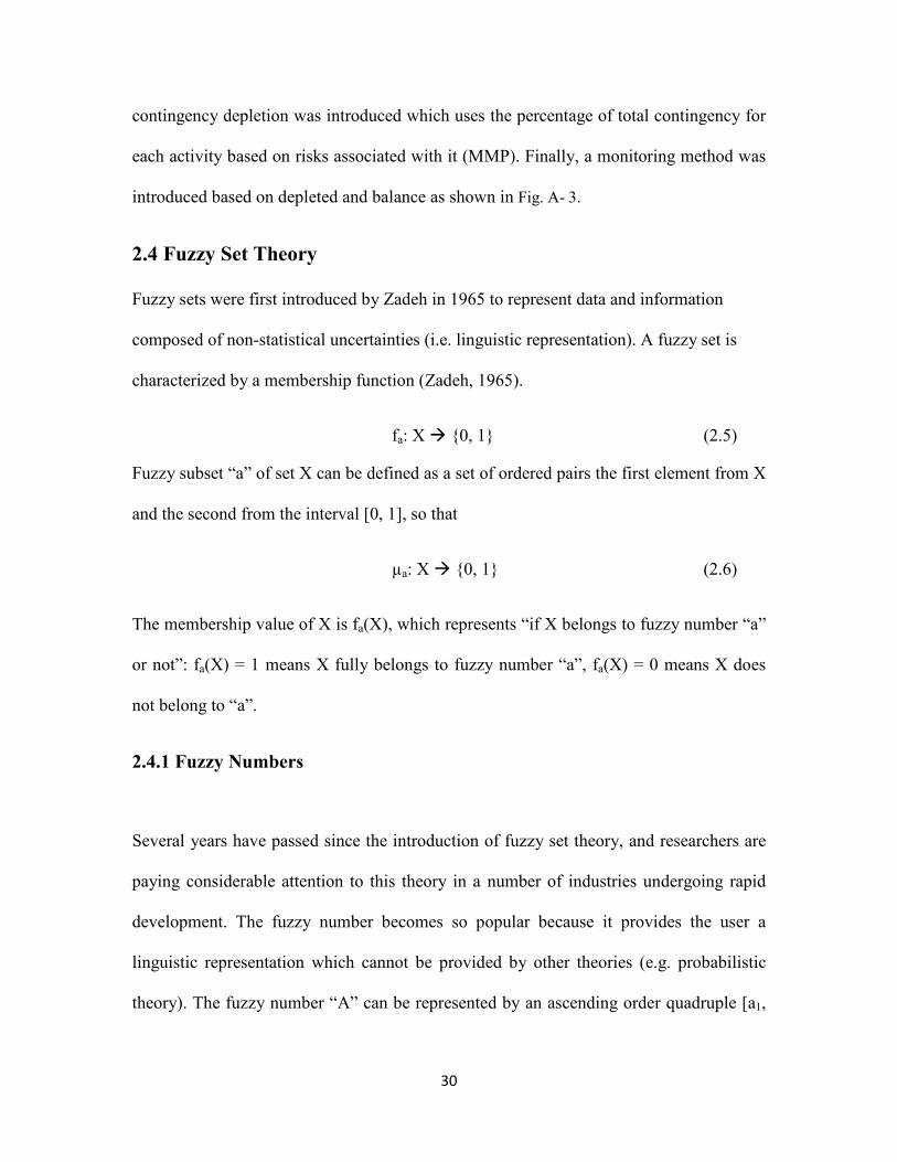
2.4 Fuzzy Set Theory
Fuzzy sets were first introduced by Zadeh in 1965 to represent data and information
composed of non-statistical uncertainties (i.e. linguistic representation). A fuzzy set is
characterized by a membership function (Zadeh, 1965).
fa: X {0, 1} (2.5)
Fuzzy subset “a” of set X can be defined as a set of ordered pairs the first element from X
and the second from the interval [0, 1], so that
µa: X {0, 1} (2.6)
The membership value of X is fa(X), which represents “if X belongs to fuzzy number “a”
or not”: fa(X) = 1 means X fully belongs to fuzzy number “a”, fa(X) = 0 means X does
not belong to “a”.
2.4.1 Fuzzy Numbers
Several years have passed since the introduction of fuzzy set theory, and researchers are
paying considerable attention to this theory in a number of industries undergoing rapid
development. The fuzzy number becomes so popular because it provides the user a
linguistic representation which cannot be provided by other theories (e.g. probabilistic
theory). The fuzzy number “A” can be represented by an ascending order quadruple [a1,
31
a2, a3, a4]. Based on the fuzzy number quadruple’s values, four types of fuzzy numbers
can be identified:
1. A Crisp Fuzzy Number: when all quadruple values are equal [a1=a2=a3=a4]. Also
called a singleton.
2. A Uniform Fuzzy Number: when the first and second values are equal and third
and fourth values are equal (a1=a2 and a3=a4).
3. A Triangular Fuzzy Number: when two or three consecutives values of the fuzzy
number’s quadruple are equal (a2=a3, a1=a2=a3, a2=a3=a4).
4. A Trapezoidal Fuzzy Number: the general form of a fuzzy number, when all the
quadruple’s values are in ascending order (a1>a2>a3>a4).
Each fuzzy number is defined by its characteristic membership function. In general the
membership function is represented by µA (Zadeh, 1965):
µA(t) =
⎩⎪⎨
⎪⎧1 𝑤ℎ𝑒𝑛, 𝑎2 < 𝑡 < 𝑎3
0 < 𝑣𝑎𝑙𝑢𝑒 < 1 𝑤ℎ𝑒𝑛, �𝑎1 < 𝑡 < 𝑎2
𝑜𝑟𝑎3 < 𝑡 < 𝑎4
0 𝑂𝑡ℎ𝑒𝑟𝑤𝑖𝑠
(2.7)
Classical set theory can be extended to fuzzy set theory. Suppose A [a1, a2, a3, a4] and B
[b1, b2, b3, b4] are two fuzzy numbers. The application of the classical set operations (Fig.
2.2) could be then expressed as:
Intersection
µA∩B (t) = min [µA(t), µB(t)] (2.8)
Union
32
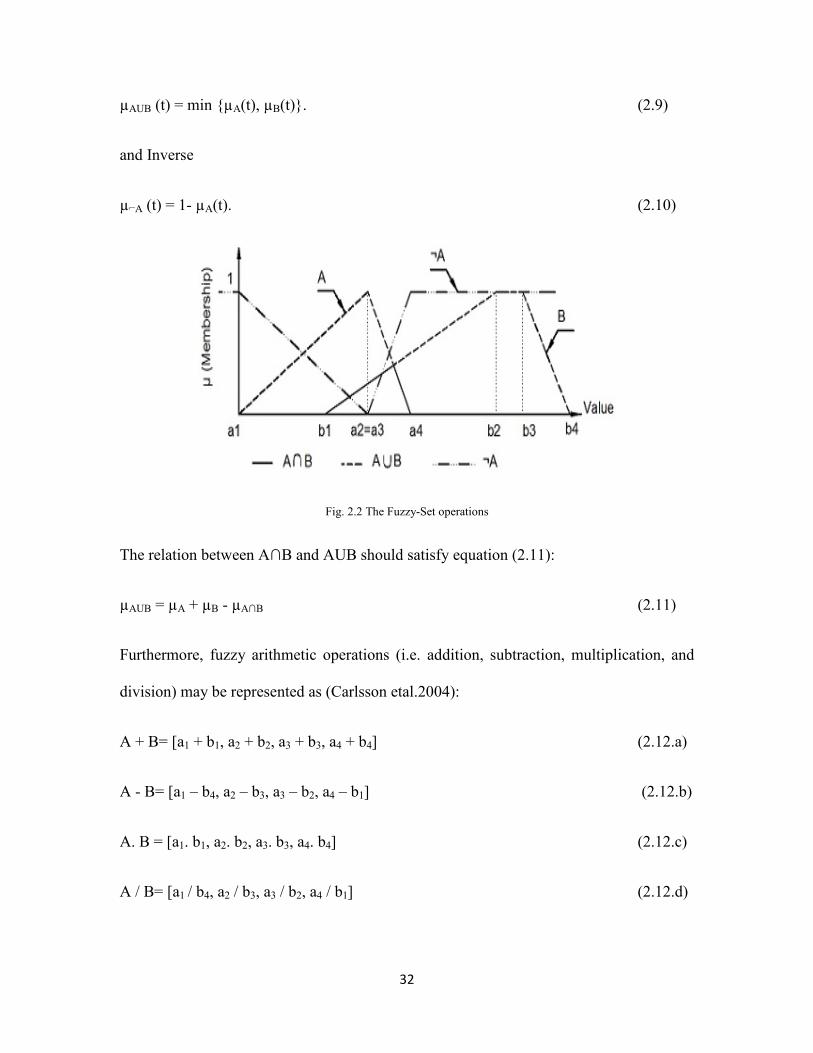
µAUB (t) = min {µA(t), µB(t)}. (2.9)
and Inverse
µ⌐A (t) = 1- µA(t). (2.10)
Fig. 2.2 The Fuzzy-Set operations
The relation between A∩B and AUB should satisfy equation (2.11):
µAUB = µA + µB - µA∩B (2.11)
Furthermore, fuzzy arithmetic operations (i.e. addition, subtraction, multiplication, and
division) may be represented as (Carlsson etal.2004):
A + B= [a1 + b1, a2 + b2, a3 + b3, a4 + b4] (2.12.a)
A - B= [a1 – b4, a2 – b3, a3 – b2, a4 – b1] (2.12.b)
A. B = [a1. b1, a2. b2, a3. b3, a4. b4] (2.12.c)
A / B= [a1 / b4, a2 / b3, a3 / b2, a4 / b1] (2.12.d)

33
In addition, the multiplication of a fuzzy number with a real number λ could be
represented as (Carlsson et al. 2004):
�λ. A = [ λ. a1 , λ. a2 , λ. a3 , λ. a4] if λ ≥ 0
𝑜𝑟λ. A = [λ. a4 , λ. a3 , λ. a2 , λ. a1] if λ < 0
(2.13)
2.4.2 Defuzzification
A fuzzy number can be represented by a crisp value after defuzzfication. The defuzzified
value represents the expected value of a fuzzy number. There are several methods for the
defuzzfication of a fuzzy number:
• Center of gravity, also called the center of area (COA): the centroid distance of a
fuzzy number, calculated by different methods as follows:
y∗ =∫ xµi(xi)∫µi(xi)
(2.14.a)
• Center of gravity weighted by area: this method it is the same of the above
method but it can be calculated to defuzzify multiple fuzzy numbers by using a
modified formula (Amaya , 2009)
COA =∑ COAi × Areaii=ni=1∑ Areaini=1
(2.14.b)
• Center of gravity weighted by height or membership: this method is very similar
to COA weighted by area except it use height weighting instead of area
weighting:

34
COA =∑ COAi × µii=ni=1∑ µini=1
(2.14.c)
• Points of maximum criterion weighted by area: uses the point of maximum in a
fuzzy set and weights it with the area of the same set as follows:
X =∑ xi × Areaini=1∑ Areaini=1
(2.14.d)
Where, X is the defuzzified value and x(i) and area(i) are the value at the
maximum point (or maximum membership) and the area of fuzzy number I,
respectively.
• Points of maximum criterion weighted by height: same as the above methods but
uses the height for weighting instead of the area:
X =∑ xi × µini=1∑ µini=1
(2.14.e)
• Average of centers: is the average of the centers of gravity of each fuzzy number:
X =∑ COAini=1
n (2.14.f)
The most commonly used method is the center of area (COA) which calculates the fuzzy
number expected value as the centroidal distance of the area. This value is also called a
fuzzy number’s deffuzified value.
y∗ =∫ xµi(xi)∫µi(xi)
(2.15)
Where, y* = defuzzified value; μ(x) = the aggregated membership function; and x = the
output variable.

35
2.4.3 Expected Value and Variance Calculations
In probability theory: mean value and variance are centroid distance and centroid moment
of inertia respectively. Several researchers have focused on the expected value and
variance of fuzzy number calculation, such as Wang and Tian, 2010; Shaheen et al, 2007;
Liu and Liu, 2002; Dorp and Kotz, 2003; Li et al., 2010; and Carlsson et al., 2004. These
researchers have all calculated fuzzy number expected value as the centroid distance of a
fuzzy number but not all of them came out with same formula ( i.e. Shaheen et al.(2007);
Wand and Tian.(2010)). In this research, the expected value will be calculated using
fuzzy set theory and the basic mathematics of integration theory.
Let A [a, b, c, d] be a general fuzzy variable with membership function. Assuming this is
increased on] -∞,x0] and decreased on[x0, +∞ [then, the expected value of “A” can be
calculated as follows:
EV = x0 −12� µ(x). dx +
x0
−∞
12� µ(x). dx+∞
x0
(2.16)
Where, x0 represents when μ(x) changes its sign from an increasing function to a
decreasing function. Based on equation (2.15) and trapezoidal fuzzy number shape,
equation (2.16) could be re-written as follows:
• If we suppose that μ(x) is increased up to b and then decreased,
EV = c −12�µ(x). dx +
12�1. dxc
b
+b
a
12�µ(x). dxd
c
(2.16.a)
• If we suppose that μ(x) increased up to c and then decreased,
36
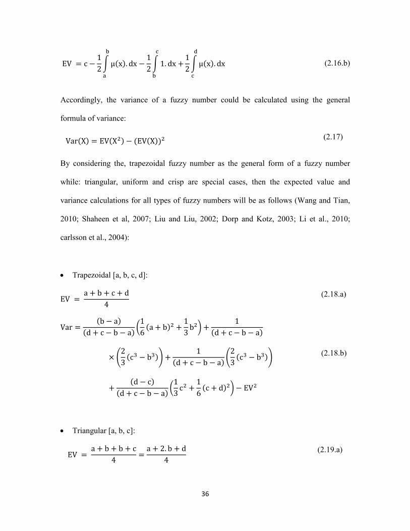
EV = c −12�µ(x). dx −
12�1. dxc
b
+b
a
12�µ(x). dxd
c
(2.16.b)
Accordingly, the variance of a fuzzy number could be calculated using the general
formula of variance:
Var(X) = EV(X2) − (EV(X))2 (2.17)
By considering the, trapezoidal fuzzy number as the general form of a fuzzy number
while: triangular, uniform and crisp are special cases, then the expected value and
variance calculations for all types of fuzzy numbers will be as follows (Wang and Tian,
2010; Shaheen et al, 2007; Liu and Liu, 2002; Dorp and Kotz, 2003; Li et al., 2010;
carlsson et al., 2004):
• Trapezoidal [a, b, c, d]:
EV = a + b + c + d
4 (2.18.a)
Var =(b − a)
(d + c − b − a) �16
(a + b)2 +13
b2� +1
(d + c − b − a)
× �23
(c3 − b3)� +1
(d + c − b − a)�23
(c3 − b3)�
+(d − c)
(d + c − b − a) �13
c2 +16
(c + d)2� − EV2
(2.18.b)
• Triangular [a, b, c]:
EV = a + b + b + c
4=
a + 2. b + d4
(2.19.a)

37
Var =a² + b² + c² − a. b − a. c − b. c
18
(2.19.b)
• Uniform [a, b]:
EV = a + a + b + d
4=
a + b2
(2.20.a)
Var =(b − a)²
12
(2.20.b)
• Crisp [a]:
EV = a + a + a + a
4= a (2.21.a)
Var = 0 (2.21.b)
Based on the fuzzy theory advantages and the limitations of existing methods for
contingency estimation fuzzy theory is selected for contingency estimating method
development in this research. In addition, non-documented methods or procedures for
contingency management represent an excellent motivation to propose a contingency
management method which could overcome other methods’ limitations. This research
will produce 1) a new method for contingency estimation based on fuzzy system
equations, 2) a new procedure for contingency management or depletion, and 3) a
depletion curve selection procedure. The proposed contingency management
methodology will be based on the practice procedures followed by project managers,
government agencies, and private companies. The proposed methodologies for
contingency estimating and management will be explicitly addressed in chapter 3.

38
CHAPTER THREE
DEVELOPED METHODOLOGY
3.1 Introduction
This chapter describe the developed method for contingency estimating using fuzzy set
theory and the method developed for contingency management using different depletion
curves applied in practice along with project managers’ strategy, procedures and
guidelines of government agencies and construction management companies. The
research model can be represented as follows:
Fig. 3.1 Contingency Estimating and Management Model
39
The literature review justified the need for a new method for contingency estimating. To
overcome the current methods’ limitations this research offers a simple and direct
contingency estimating method. Usually, project teams (i.e. project managers and
estimators) try to avoid applying a new method for reasons such as: 1) complexity,
especially if an experienced user is needed; and 2) anticipated low accuracy (not
considerable) of a new method compared to the method currently used. Both these
reasons have been eliminated by the proposed method, as well as others, as it is: 1)
simple, 2) accurate, 3) direct, and 4) applicable without the need for historical data
records.
The proposed contingency management method is needed to fill the gap between
contingency estimating, allocation, and management. Since the subjectivity of decision
makers in contingency management justifies the project managers’ use of gut-feel
decisions, these are normally based on the project managers’ past experience in similar
projects. In addition, the common practice considers contingency as an untapped fund
and that it should be kept hidden from others (except for the person who has the authority
to deplete it, i.e. the project manager) in order to avoid its misuse (Risner, 2010).
3.2 Contingency Estimating
The implementation of the proposed method for contingency estimating encompasses the
execution of the following operations:
Fuzzification:
Cost items are represented by fuzzy numbers based on expert judgment. The outputs of
fuzzification are the fuzzy estimates Aij for each cost item Ai given by each expert Ej.

40
𝑊ℎ𝑒𝑟𝑒, �i = 1 . . . n, n is number of cost items j = 1 … m, m is number of experts participatedin estimating cost item Ai
Unifying Inputs:
The outputs of the fuzzification have been re-expressed as trapezoidal fuzzy numbers to
satisfy the proposed method’s input criteria. A unifying procedure generates the
quadruples of the cost item’s fuzzy estimates by expressing: 1) a crisp fuzzy number as
[a, a, a, a] instead of [a], 2) a uniform fuzzy number as [a, a, b, b] instead of [a, b] and 3)
a triangular fuzzy number as [a, b, b, c] instead of [a, b, c].
The fuzzy contingency estimating is carried out at the cost item, work package and
project levels. At the cost item level, the fuzzy estimate is calculated as average of all the
fuzzy estimates given by participating experts:
Ai = � Aij
j=mi
j=0
(3.1.a)
Ai =1
mi�� aij, � bij,
j=mi
j=0
� cij,j=mi
j=0
j=mi
j=0
� dij
j=mi
j=0
� (3.1.b)
Ai = �1
mi� aij,
1mi
� bij,1
mi
j=mi
j=0
� cij,1
mi
j=mi
j=0
j=mi
j=0
� dij
j=mi
j=0
� (3.1.c)
At the package level, the fuzzy estimate of a package that contains ni cost items Ai (i= 1...
ni), may be calculated as the sum of all its cost items’ fuzzy estimates:
Pk = � Aik
i=n𝑖
i=1
(3.2)

41
At the project level, the fuzzy estimate of a project that contains np packages Pk (k= 1…n)
in the project range cost estimate can be calculated as the sum of all its packages’ fuzzy
estimates:
C = � Pk
k=np
k=0
(3.3)
Where, Ai, Pk, and C are the fuzzy estimates of the activity, the package, and the project
respectively.
Defuzzification
The fuzzy number’s expected value and variance values are considered as the defuzzified
values of the fuzzy number, similar to the probability theory. The expected value and
variance formulas described in section 2.4.3 could be used to defuzzify the fuzzy
estimates calculated in the previous step. The expected value can be calculated based on
the estimating level (i.e. cost item, package, or project level) as follows:
• Cost Item Expected Value: two methods can be used to calculate the expected value
of the cost item, either by:1) using the expected value of the fuzzy cost item’s
estimate [𝐸𝑉(𝐴𝑖)], or 2) using the average of the expected values of the cost item’s
fuzzy estimates given by experts [1𝑛𝐸𝑉(𝐴𝑖𝑗)), where n is the number of experts
participating in the cost item 𝐴𝑖 estimation process.
• Package Expected Value: can be calculated as either: 1) the expected value of the
package fuzzy estimates [𝐸𝑉(𝑃𝑘)], or 2) the sum of all the expected values of the cost
items associated with this package [∑ 𝐸𝑉(𝐴𝑖𝑘)𝑛𝑖𝑖=1 ], where ni is the number of cost
items included in the package.

42
• Project Expected Value: can be calculated: 1) as the expected value of the project’s
fuzzy estimate [𝐸𝑉(𝐶)], or 2) as the sum of the packages’ expected value
[∑ 𝐸𝑉(𝑃𝑘)𝑛𝑝𝑘=1 ], where np is the number of packages included in the project.
The variance of a fuzzy number may be calculated based on the estimating level (i.e. cost
item, package, or project level) and on the fuzzy number’s type. The fuzzy number’s
variance can be calculated using the variances’ formulas expressed in section 2.4.3.
Uncertainty Modeling
Uncertainty may be represented by introducing a number of measures, indices and ratios.
In this thesis several measures extracted from the literature will be incorporated, such as:
fuzziness (Klir and Fogler, 1988), ambiguity (Delgado et al., 1998), possibility (Dubois et
al., 2004), necessity (Dubois et al., 2004), mλ (Dubois et al., 2004), a fuzzy number
quality index (FNQI) (Shaheen et al., 2007), and an agreement index (Sakawa and Mori,
1999). In addition, this research introduces two ratios: the fuzziness expected value ratio,
and the ambiguity expected value ratio. These two units-less ratios improve the ability of
the contingency estimator to check the results’ quality (i.e. to what extent the results are
fuzzy and ambiguous).
The extracted and proposed uncertainty measures will support decision making by
providing reliable information about several expected scenarios. It also indicates the
quality and reliability of such information. The contingency estimation model introduced
in this thesis can be represented by three sub-models:1) data gathering, 2) fuzzy
estimating, and 3) defuzzification, which also includes the calculation of all the
aforementioned uncertainty modeling (i.e. measures, indices and ratios) as shown Fig. 3.2.

43
Fig. 3.2 Contingency Estimation Model
3.3 Uncertainty Quantification
3.3.1 Uncertainty Measures
The fuzziness measure was introduced by Klir and Fogler (1988); it can be considered as
the degree of lack of distinction between the presentation of a fuzzy number and its
complement. If it is difficult to distinguish between a fuzzy number and its complement
then the maximum fuzziness is associated with that fuzzy number, otherwise, less

44
fuzziness is associated with it. This measure may reach “0” if the fuzzy number is crisp
or uniform. The fuzziness measure can be calculated using the formula (Shaheen et al.
2007)
F(A) = � (1 − |2µA(x) − 1|) dx+∞
−∞ (3.4)
The above integral can also be solved using integration by parts to simplify the
calculation formula of the fuzzy number’s fuzziness measure as follows so that:
F(A) = � dx+∞
−∞− � |2µA(x) − 1| dx
+∞
−∞
F(A) = � dx+∞
−∞− � |2µA(x) − 1| dx
a
−∞− � |2µA(x) − 1| dx
b
a− � |2µA(x) − 1|dx
c
b
+ � |2µA(x) − 1| dxd
c+ � |2µA(x) − 1|dx
+∞
d
Since,
⎩⎪⎨
⎪⎧µA(x) = 0 when x < 𝑎 µA(x) = x−a
b−a when a < 𝑥 < 𝑏
µA(x) = 1 when b < 𝑥 < 𝑐µA(x) = x−d
c−d when c < 𝑥 < 𝑑
µA(x) = 0 when x > 𝑑
⎩⎪⎨
⎪⎧ ∫ (1− �2µA(x) − 1|) dx a
−∞ = 0and
∫ (1− �2µA(x)− 1|) dx +∞d = 0
and∫ dx+∞−∞ = ∫ dxb
a + ∫ dxcb + ∫ dx d
c
While,
� dx+∞
−∞= � dx
b
a+ � dx
c
b+ � dx
d
c= b − a + c − b + d − c = d − a
Then F (A) can be re-written as follows:
F(A) = d − a −� |2µA(x) − 1| dx b
a− � |2µA(x) − 1| dx
c
b− � |2µA(x) − 1| dx
d
c
Solving each integral separately:
� |2µA(x) − 1| dx b
a= � (2µA(x) − 1)dx
a+b2
a+ � �1 − 2µA(x)�dx
b
a+b2

45
� |2µA(x) − 1| dx b
a= � �2 ×
x − ab − a
− 1� dxa+b2
a+ � �1 − 2 ×
x − ab − a
�dxb
a+b2
� |2µA(x) − 1| dx b
a= � �
2xb − a
−b + ab − a
�dxa+b2
a+ � �
b + ab − a
−2x
b − a�dx
b
a+b2
� |2µA(x) − 1| dx b
a=
x²b − a
−b + ab − a
x�a+b2
a+
b + ab − a
x −x²
b − a�
ba+b2
� |2µA(x) − 1| dx b
a=
b − a4
+b − a
4=
b − a2
Similarly, for the interval [c, d]
� |2µA(x) − 1| dx d
c=
d − c2
Moreover, the membership µA(x) = 1 when 𝑥 ∈ [𝑏, 𝑐] 2µA(x) − 1 = 1
� |2µA(x) − 1| dx c
b= � 1 dx
c
b= x ]
𝑐𝑏
= c − b
Equation (3.4) can therefore be updated as follows:
F(A) = d − a +a − b
2+ b − c +
c − d2
By simplifying, the general formula of the fuzziness measure can be expressed as:
F(A) = (b − a) + (d − c)
2 (3.4.a)
The ambiguity measure was introduced by Delgado et al. (1998 a), and can be calculated
using the following formula (Delgado et al. 1998a):
AG(A) = � r[R(r) − L(r)]1
0
dr (3.5)
However, the general formula for the fuzzy number’s ambiguity measure can also be
generated using the integration theory. By definition, R(r) and L(r) are the left and right

46
functions of a fuzzy number with LR-type representation (another fuzzy number
representation) which can be described as follows (Carlsson et al., 2004):
A(t) =
⎩⎪⎪⎪⎨
⎪⎪⎪⎧L(
b − tb − a
), 𝑡 ∈ [𝑎, 𝑏]
1, 𝑡 ∈ [𝑏, 𝑐]
R(t − cd − c
), 𝑡 ∈ [𝑐,𝑑]
0, otherwise
(3.6)
Where, L(r) and R(r) represent the r-cut representation of µA. Let us assume A is a
trapezoidal fuzzy number which means L(r) and R(r) could be represented as follows:
L(r) = [b − r(b − a)] (3.7)
R(r) = [r(d − c) + c] (3.8)
Equation (3.5) could thus be re-written as follows:
AG(A) = � r[(r(d − c) + c) − (b − r(b − a))]1
0
dr
AG(A) = �(r2(d − c) + cr )1
0
dr −�(br − r²(b − a)1
0
dr
AG(A) = �r3
3(d − c) +
cr2
2�1
0� − �
r3
3(b − a) +
br2
2�1
0�
AG(A) = �(d − c)
3+
c2� − �
(b − a)3
+b2�
By simplifying, a general formula for the trapezoidal fuzzy number’s ambiguity measure
could be generated as shown below:

47
AG(A) =d + 2c − 2b − a
6 (3.9)
Based on equations “3.4.a” and “3.9”, the fuzziness and ambiguity measures for most
common fuzzy numbers can be calculated using the formulas presented in Table 3.1:
Table 3.1 Fuzziness and Ambiguity Measures Calculations
Fuzzy Number Type Fuzziness Measure Ambiguity Measure
Crisp [a] 0 0
Uniform [a, b] 0 b − a2
Triangular [a, b, c] c − a
2
c − a6
Trapezoidal [a, b, c, d] (b − a) + (d − c)2
d + 2c − 2b − a
6
The possibility measure was introduced by Zadeh (1965). It has since been used by many
other researchers. By definition, it measures how likely a fuzzy number A will belong to
a specific interval [m, n]. Let A be a fuzzy variable with membership function μA(x), and
[m,n] an arbitrary interval in ℝ (reel set). Then, the possibility measure of a fuzzy event
{A ∈ [m, n]} could be expressed as follows (Dubois et al., 2004; Yang and Iwamura,
2008):
Pos{A ∈ [m, n]} = Supx∈[m,n]
(µA(x)) (3.10)
The necessity measure satisfies properties that are similar to the possibility measure with
respect to set-intersection, and it can be calculated as the impossibility of opposite event.
For example, let A be a fuzzy variable with membership function μA(x), and [m, n] an

48
arbitrary interval in ℝ (reel set). The necessity measure will be expressed as follows
(Dubois et al., 2004):
Nec{A ∈ [m, n]} = 1 − Supx∉[m,n]
(µA(x)) (3.11)
The possibility and necessity measures represent the optimistic and the pessimistic
decision maker, respectively. Therefore, it is important to combine the both measures
with a new measure (mλ) which represents a normal decision maker. The combined
measure mλ could be represented as follows:
mλ = λ × Pos{A} + (1 − λ)Nec{A} (3.12)
where λ is a number ∈ [0, 1] that represents the optimism characteristic of the decision
maker:
if �λ = 0,→ pessimistic decision maker → mλ = Nec(A)λ = 1,→ optimistic decision maker → mλ = Pos(A) 0 < 𝜆 < 1,→ Otherwise → Nec(A) < 𝑚λ < 𝑃𝑜𝑠(𝐴)
(3.12.a)
For a neutral decision maker with λ=0.5 (neither optimistic nor pessimistic) the mλ
measure may be expressed as:
mλ =Nec(A) + Pos(A)
2 (3.12.b)
3.3.2 Uncertainty Ratios
The fuzziness expected value ratio (FER) can be represented by the ratio of the fuzziness
measure to the expected value of a fuzzy number “A”. This ratio could be expressed as:
FER(A) =F(A)
EV(A) (3.13)
49
Similarly, the ambiguity expected value ratio (AER) is a ratio of the ambiguity measure
of a fuzzy number “A” over its expected value. This ratio could be expressed as:
AER (A) =AG(A)EV(A)
(3.14)
These ratios are unit-less and they represent the fuzziness and the ambiguity percentage
of the fuzzy number’s expected value. These two ratios indicate the quality of the fuzzy
number’s estimate more accurately than do the fuzziness and the ambiguity measures on
their own.
3.3.3 Uncertainty Indices
This methodology includes two types of indices: (1) the fuzzy number quality index
(FNQI), and (2) the agreement index (AI). Shaheen et al. (2007) introduced the FNQI to
combine the effects of the fuzziness measure and the ambiguity measure. This index may
be calculated as the weighted average of both measures (fuzziness and ambiguity) as
follows (Shaheen et al. 2007):
FNQI = WF × F(A) + WAG × AG(A)
WF + WAG (3.15)
Where, WF and WAG represent the weights of the fuzziness measure and the ambiguity
measure respectively. This index helps to eliminate the non-reliable inputs, as they will
have higher FNQI values than other inputs (Shaheen et al., 2007).
The agreement index (AI) represents the agreement percentage between two fuzzy
numbers. It was calculated by Sakawa and Mori (1999) as the ratio of the intersection
area of two fuzzy numbers’ memberships over the area of the first fuzzy number
membership. This index can be expressed as follows (Sakawa and Mori, 1999):

50
AI (A, B) =Area (A ∩ B)
Area A (3.16)
The agreement index has a maximum value equal to 1 when A∩B=A.
These measures, indices, and ratios were selected and incorporated in the proposed
methodology. In general, uncertainty modeling (including all of these measures)
maximizes the user’s ability to control the inputs by providing useful information about
the quality of the inputs (i.e. FNQI) and outputs (i.e. FER).
3.4 Contingency Management The effort required to manage a project’s contingency is related to the project’s allocated
contingency fund volume (Ruskin 1981). For example, if the allocated contingency fund
volume is relatively high (i.e. 50% of a project’s cost), the management effort required to
manage the contingency varies from limited to negligible. In contrast, if the allocated
contingency fund is relatively low (i.e. <5% of a project’s cost) then, the management
effort required would have to be considerably aggressive (Ruskin, 1981).
The proposed method for contingency management is based on a contingency depletion
curve. It was noted that the selection of a contingency’s depletion curve depends on
several factors. Therefore, this research extracts all the factors that affect contingency
depletion utilizing a range of sources including the literature, associations’ policies,
companies’ practices, and project managers’ applications.
3.4.1. Factors Affecting Contingency Depletion
Both the literature and practices show that there are several factors affecting contingency
depletion. These factors are: 1) project type (U.S. DOE, 2006), 2) complexity (U.S. DOE,
51
2006), 3) risk impact and severity (Washington TRU Solutions LLC, 2008), 4) type of
occurred risk (U.S. DOE, 2009), and 5) management strategy or approach (Ruskin,
1981).
Project Type
The project type is a very important factor since the contingency management of an
infrastructure project could be very different from that of a tunneling or a building
project. Project type is closely connected to contract type, since lump sum contracts are
more risky than unit price contracts, cost plus contracts, and cost plus-plus contracts,
especially for contractor. The availability of reliable information about a project and its
associated difficulties increases the contingency manager’s ability to deplete
contingency as planned. Otherwise, the contingency manager is obliged to avoid the
early depletion of contingency and especially be aware of the unforeseen risks which
may occur over a project’s duration. In addition, a contractor’s experience in similar
projects decreases the amount of unforeseen or unplanned risks and it can eliminate
contingency depletion fuzziness. Therefore, the project’s type is considered an
important factor that affects the contingency depletion.
Complexity
The complexity factor seems to be related to a project’s type, but complexity can be
addressed from different perspectives such as: 1) a fast-track delivery system, 2)
technical difficulties, and 3) the requirements of new technology. The project complexity
should be considered by the contingency manager up to the point where the fuzziness
associated with the project’s complexity is eliminated.
52
Risk Impact (Severity)
The risk impact, called also cost-benefit tradeoff, is considered an important factor that
affects contingency depletion. For example if the impact of an occurred risk has a very
low effect, then, the use of contingency to mitigate this risk would be meaningless and
actually have no value for the project. Likewise, if the allocated contingency for the
mitigation of occurred risk not enough to compensate (project risk tolerance) and the
mitigation’s cost-benefit tradeoff (in monetary value) is less than the additional
contingency that would be required, then, the use of contingency for this situation would
not make economic sense and is not recommended.
Type of Risk Occurred
Different types of risk can be found in the literature including technical, scheduling,
resources (labor, material, machinery, support services etc…), financial (rate change,
interest, inflation etc…), technological, political, and country-based. Each type can be
managed using different approaches especially when a risk would have a considerable
impact and uncertain consequences (i.e. politics, technical difficulty, technology
availability).
Management Skills and Strategy
The management skills of a project’s manager and his/her depletion strategy (passive or
aggressive) affect contingency depletion. According to Ford (2002), each strategy has its
advantages and disadvantages. The project manager (contingency manager) usually
makes a subjective decision about the selected strategy’s advantages over other strategies
(Ford 2002). The project manager’s selection is difficult to defend since it does not

53
follow any systematic procedure. The selection of a project manager’s strategy thus
affects the contingency’s depletion.
3.4.2 Proposed Depletion Curves
In the literature there are strategies, subjective procedures, and contingency depletion
applications based on experience. The use of the depletion curve methodology is limited
to the basic depletion curve (Noor and Tichacek, 2004) and the linear curve (Turner,
2011). The typical spending curve considers that contingency depletion should follow the
shape of the project cost baseline (S-curve). The linear contingency depletion curve
assumed that the contingency should be uniformly distributed over a project’s duration
(or contingency’s milestones). This research identifies four types of contingency
depletion curves (Fig. 3.3) from the literature and proposes a new depletion curve. Linear
Depletion Curve
Basically, this is the ideal depletion curve. It distributes the contingency fund between
project periods or milestones uniformly. Several companies prefer to establish a project
with a linear depletion curve as its planned depletion curve. For example Turner (2011)
used a linear depletion curve in Mitchell Park Library Community Center project for the
City of Palo-Alto in the United States (Turner, 2011).
Basic Depletion Curve (S-curve)
This curve is also called the typical spending curve (Noor and Tichacek, 2004). It
considers that the depletion of contingency should follow the project cost baseline since
all the project’s resources (i.e. man power, money, and material) are depleted
accordingly.
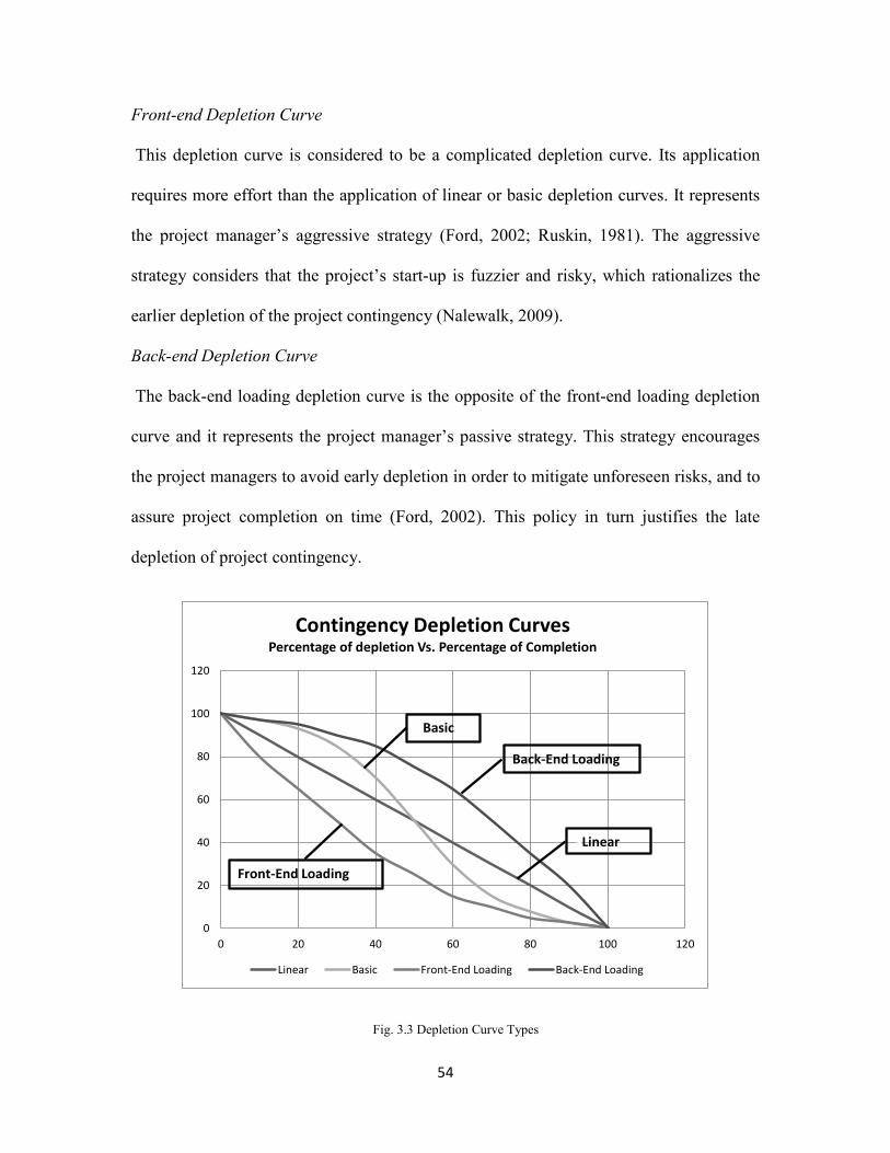
54
Front-end Depletion Curve
This depletion curve is considered to be a complicated depletion curve. Its application
requires more effort than the application of linear or basic depletion curves. It represents
the project manager’s aggressive strategy (Ford, 2002; Ruskin, 1981). The aggressive
strategy considers that the project’s start-up is fuzzier and risky, which rationalizes the
earlier depletion of the project contingency (Nalewalk, 2009).
Back-end Depletion Curve
The back-end loading depletion curve is the opposite of the front-end loading depletion
curve and it represents the project manager’s passive strategy. This strategy encourages
the project managers to avoid early depletion in order to mitigate unforeseen risks, and to
assure project completion on time (Ford, 2002). This policy in turn justifies the late
depletion of project contingency.
Fig. 3.3 Depletion Curve Types
0
20
40
60
80
100
120
0 20 40 60 80 100 120
Contingency Depletion Curves Percentage of depletion Vs. Percentage of Completion
Linear Basic Front-End Loading Back-End Loading
aBasic
aLinear
Back-End Loading
Front-End Loading
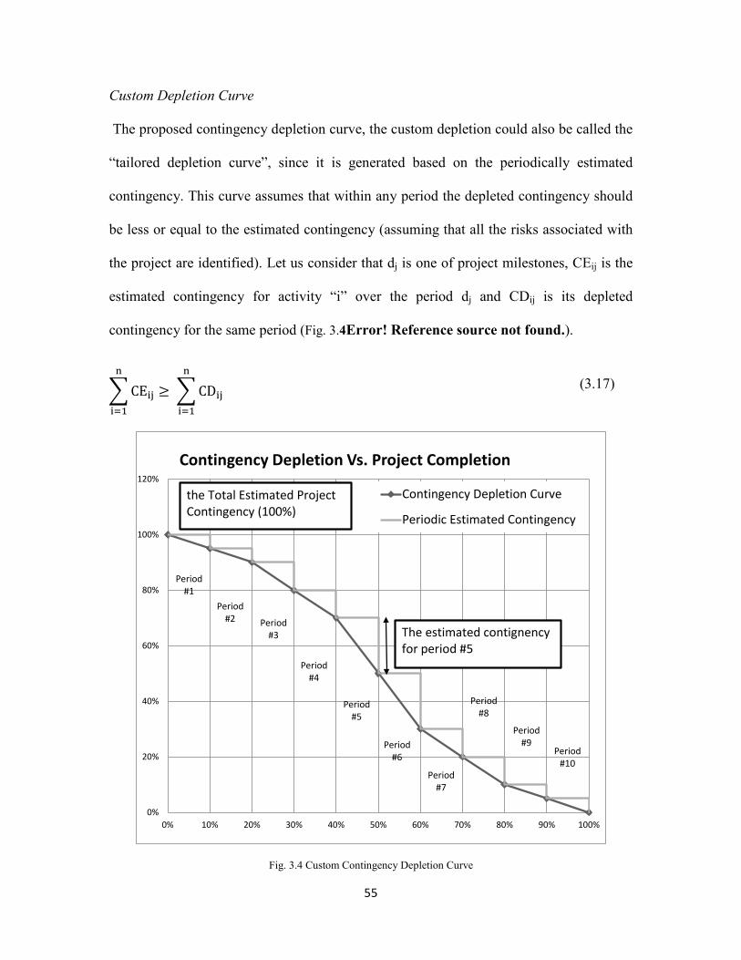
55
Custom Depletion Curve
The proposed contingency depletion curve, the custom depletion could also be called the
“tailored depletion curve”, since it is generated based on the periodically estimated
contingency. This curve assumes that within any period the depleted contingency should
be less or equal to the estimated contingency (assuming that all the risks associated with
the project are identified). Let us consider that dj is one of project milestones, CEij is the
estimated contingency for activity “i” over the period dj and CDij is its depleted
contingency for the same period (Fig. 3.4Error! Reference source not found.).
�CEij
n
i=1
≥ �CDij
n
i=1
(3.17)
Fig. 3.4 Custom Contingency Depletion Curve
0%
20%
40%
60%
80%
100%
120%
0% 10% 20% 30% 40% 50% 60% 70% 80% 90% 100%
Contingency Depletion Vs. Project Completion
Contingency Depletion Curve
Periodic Estimated Contingency
The estimated contignencyfor period #5
Period#10
the Total Estimated Project Contingency (100%)
Period#9
Period#8
Period#7
Period#6
Period#5
Period#4
Period#3
Period#2
Period#1

56
For a specific period or project milestone, the summation of depleted contingency should
be less than or equal to the summation of estimated contingency for the same period.
Assuming that during this specific period, m activities were implemented this means that:
�CDi ≤�CEi
m
i=1
m
i=1
(3.18)
As with contingency management, some of the planned risks may occur during a specific
period T and this could generate an excess in the project’s contingency. Therefore, a
reserve contingency account (RC) should receive the entire excess contingency. This
policy increases the contingency fund’s controllability by eliminating the misuse and the
over-exhaustion of contingency. The reserve contingency account could be increased or
decreased based on the difference between planned contingency (PC) and the actual
contingency (AC) during the specific period T as follows:
𝑃𝐶(𝑇) ≥ 𝐴𝐶(𝑇) (3.19)
𝑅𝐶 = 𝑅𝐶 + [𝑃𝐶(𝑇) − 𝐴𝐶(𝑇)] (3.20)
Where: PC (T) is the estimated contingency during the period T, which could also be read
from (Fig. 3.6). AC (T) could be calculated as follows:
𝐴𝐶(𝑇) = ∑ 𝐴𝐶𝑖𝑛𝑖=1 (𝑇) (3.21)
Where, ACi (T) is the actual contingency used to mitigate risk Ri during the period T, and
n is the number of risks planned during the period T.
In the cases where PC(T) < 𝐴𝐶(T), a shortage in contingency could be generated which
means the use of the contingency reserve is required. A “use reserve contingency

57
request” would then be submitted to the contingency reserve account’s manager for
approval. The contingency shortage should be covered by the use of the contingency
reserve only when the request has been approved; otherwise, an extension of contingency
(i.e. new contingency fund resource) is needed. In addition, the contingency reserve could
be used to mitigate the unforeseen risks and the unknown risks if necessary. The
contingency depletion performance could be evaluated by calculating the ratio between
planned project contingency (PC) and actual depleted contingency (AC) as follows:
⎩⎪⎪⎨
⎪⎪⎧𝐴𝐶𝑃𝐶
> 1 ⇒ 𝐶𝑜𝑛𝑡𝑖𝑛𝑔𝑒𝑛𝑐𝑦 𝑆ℎ𝑜𝑟𝑡𝑎𝑔𝑒 𝑖𝑠 𝑔𝑒𝑛𝑒𝑟𝑎𝑡𝑒𝑑
𝐴𝐶𝑃𝐶
< 1 ⇒ 𝐶𝑜𝑛𝑡𝑖𝑛𝑔𝑒𝑛𝑐𝑦 𝐸𝑥𝑐𝑒𝑠𝑠 𝑖𝑠 𝑔𝑒𝑛𝑒𝑟𝑎𝑡𝑒𝑑
𝐴𝐶𝑃𝐶
= 1 ⇒ 𝑁𝑜 𝐶𝑜𝑛𝑡𝑖𝑛𝑔𝑒𝑛𝑐𝑦 𝑠ℎ𝑜𝑟𝑡𝑎𝑔𝑒 𝑜𝑟 𝑒𝑥𝑐𝑒𝑠𝑠
This procedure could be represented as follows (Fig. 3. 5):

58
Fig. 3. 5 Contingency Management Model
The selection procedure of the contingency’s depletion curve as a “Project Planned
Contingency Depletion Curve” should take into consideration the factors that can affect
the selection (i.e. a company’s financial capacity).
The selection could be performed using the “IF-AND-THEN” approach which increases
the probability to choosing the most suitable depletion curve for a specific project. This
59
approach is governed by several rules based on: 1) experience, 2) past project learned
lessons, 3) management skills, and 4) applicability. These rules can be improved on
project basis. There are several scenarios can be presented, such as the following five:
Scenario 1: IF the project is an infrastructure project (i.e. information about the project is
not complete) AND the project manager prefers to use the aggressive strategy AND the
company’s financial capacity is good THEN the back-end loading depletion curve would
be recommended, since it improves the ability to control the project manager’s aggressive
strategy and avoid the early depletion of the project contingency (i.e. until more
information about the project becomes available).
Scenario 2: IF the project’s delivery system is fast-track AND the project manager
prefers the passive strategy AND the company’s financial capacity is very good THEN
the front-end loading depletion cure would be recommended, since it increases the ability
to control a project manager’s passiveness and encourages contingency depletion earlier
in order to avoid any project delay.
Scenario 3: IF the project information is complete and reliable AND the associated risks
with the project are well identified and evaluated AND the project financing has a
uniform cash flow AND the company’s past experience in similar projects is excellent
THEN the linear depletion curve would be recommended, since it is simple to use,
monitor and control. It could be the best-fit depletion curve in the case of uniform cash
flow.
Scenario 4: IF the company has very good experience in similar projects AND the project
financing follows the S-curve project cost baseline (i.e. same funding resources) THEN

60
the basic depletion curve would be recommended, since it follows the resources’
availability (i.e. money, manpower, machinery, materials) over the project durations and
addresses all the risks associated with them accordingly.
Scenario 5: IF the project type is conventional (i.e. Education Center) AND the
company’s financial capacity is average AND the company’s experience in similar
project is average AND the risks associated with the project are reliably evaluated THEN
tailored depletion curve would be recommended, since it eliminates the late and the
earlier depletion of contingency, and improves the ability to control contingency
depletion periodically (i.e. at any project’s milestone).
61
CHAPTER FOUR
DEVELOPED COMPUTER APPLICATION
4.1 Introduction
This chapter describes the implementation of the developed contingency estimating
method described in Chapter 3. The software called “Contingency Fuzzy System
Software” or CFSS was developed using object-oriented programming and NET
framework version 4. It was coded using visual basic VB.NET 2010. CFSS is standalone
software which can be used without the reliance on a 3rd party software or any other
external component or dynamic libraries such as. Microsoft Excel, DLL files.
CFSS includes four main modules: 1) input module, 2) fuzzy estimation module, 3)
graphical representation module, and 4) analytical reporting module. The input module
contains fuzzy contingency inputs (based on number of estimators/ experts) associated
with each risk at the cost item level. The estimation module (number 2 noted above)
includes five sub-modules: a) fuzzy estimation, b) measures, c) ratios, d) indices, e)
defuzzification value, and f) estimation with certain possibility not exceeding a specific
value. The graphical representation module (number 3 noted above) shows graphically
the fuzzy estimate of cost items, packages and project(s). The analytical reporting module
(number 4 noted above) considered the CFSS output, generates an analytical report for
either one specific project or a group of projects. The report generated includes the
information needed to monitor and control a specific cost item, package or project. The

62
CFSS model is flexible and easy to use. Project cost estimates follow detailed, risk
breakdown structure (RBS), which can be described as shown in (Fig. 4.1)
Fig. 4.1 Fuzzy Contingency Estimation Model
Each cost item (risk) can have a different number of fuzzy estimates based on the number
of experts participating in the cost item’s estimation process. The fuzzy estimate of each
risk item is calculated as average of all estimates provided. The fuzzy estimate of each
activity is calculated as (sum of fuzzy estimates of risks) / (cost of items associated with
this activity). The fuzzy estimate of project is the sum of fuzzy estimates of all project
activities.
63
4.2 Characteristics of the Developed Application
CFSS uses a Graphical User Interface (GUI); coded in VB.NET. The software allows
users to input data with different methods: 1) New Data Entry, this method used when a
new category is implemented and the majority of inputs can’t be imported from an
existed or saved data. 2) Loading an incomplete data: used to load incomplete data entry
file in order to complete the same. 3) Importing Data from an existing Project: data will
imported from an existing project with the ability to join the new and existing data at any
phase. The software’s main screen is shown in (Fig. 4. 2).
The software is user-friendly and it doesn’t need any experience or training to use it. The
interactive screens, between the software and the instructions, provided to user are
capable of limiting the errors associated with input.
This software is limited to 3-level of details: cost item, package and project. However, it
could be expanded to introduce more levels. The complicated calculations are hidden to
limit the inexperienced user’s confusion. Besides that, CFSS has a user-friendly output in
a readable and well organized format. The software has a graphical representation in
order to simplify the output.
Given that this is stand-alone software, the setup of the software can be done easily. The
software works in a windows environment with a net framework installed on it.

64
Fig. 4. 2 Contingency Fuzzy System
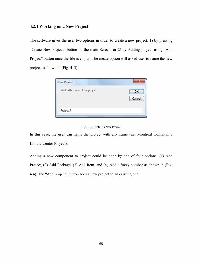
65
4.2.1 Working on a New Project
The software gives the user two options in order to create a new project: 1) by pressing
“Create New Project” button on the main Screen, or 2) by Adding project using “Add
Project” button once the file is empty. The create option will asked user to name the new
project as shown in (Fig. 4. 3).
Fig. 4. 3 Creating a New Project
In this case, the user can name the project with any name (i.e. Montreal Community
Library Center Project).
Adding a new component to project could be done by one of four options: (1) Add
Project, (2) Add Package, (3) Add Item, and (4) Add a fuzzy number as shown in (Fig.
4.4). The “Add project” button adds a new project to an existing one.

66
Fig. 4.4 Adding a New Component

67
The “Add package” button shows an interactive screen which asks the user to enter the
package name as shown in (Fig. 4.5). There is one condition prior to add a package: 1)
the user should select a project node, otherwise an interactive screen show up and asked
him to select a project node first as shown in (Fig. 4.6).
Fig. 4.5 Adding a Package
Fig. 4.6 Adding Package Error
The “Add Item” button (Fig. 4.4) asked the user to enter the cost item’s name as shown in
(Fig. 4.7). There is one condition prior to add a cost item: 1) the user should select a
package node, otherwise an interactive screen show up and asked him to select a package
node first as shown in (Fig. 4.8).
Fig. 4.7 Adding a Package
Fig. 4.8 Adding Item Error
The “Add Item” button (Fig. 4.4) asks the user to enter a cost item’s fuzzy estimate as
shown in (Fig. 4.9). There is on one condition prior to add a fuzzy number: 1) the user
should select a cost item node, otherwise one of two interactive screens, based on the
error, will occur. There are two types of errors: 1) input error (Fig. 4.10) which indicates
that the user didn’t follow the instructions and correct input as mentioned in (Fig. 4.9), 2)
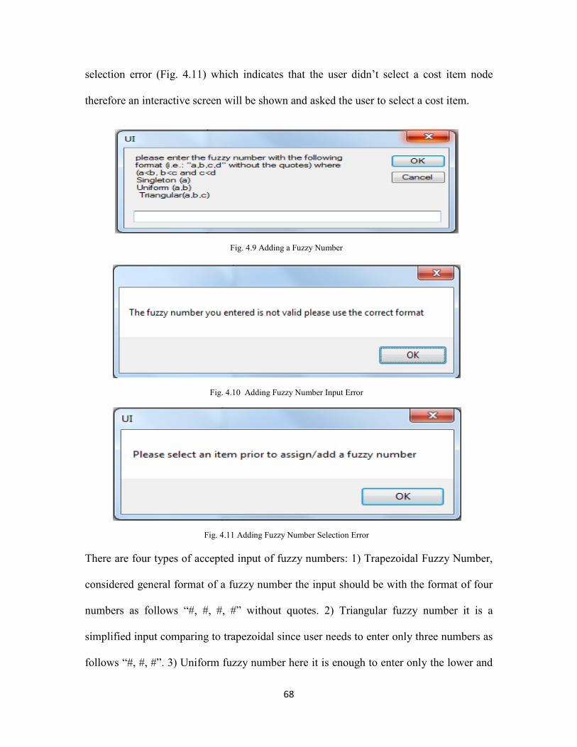
68
selection error (Fig. 4.11) which indicates that the user didn’t select a cost item node
therefore an interactive screen will be shown and asked the user to select a cost item.
Fig. 4.9 Adding a Fuzzy Number
Fig. 4.10 Adding Fuzzy Number Input Error
Fig. 4.11 Adding Fuzzy Number Selection Error There are four types of accepted input of fuzzy numbers: 1) Trapezoidal Fuzzy Number,
considered general format of a fuzzy number the input should be with the format of four
numbers as follows “#, #, #, #” without quotes. 2) Triangular fuzzy number it is a
simplified input comparing to trapezoidal since user needs to enter only three numbers as
follows “#, #, #”. 3) Uniform fuzzy number here it is enough to enter only the lower and

69
upper bound “#, #”, 4) Crisp fuzzy number it is the easiest since user is requested to enter
only one number “#”.
All these instructions are incorporated to simplify the user’s input and decrease the time
required for data input. The software will automatically identify the fuzzy number’s type
and generate the equivalent quadruple of triangular, uniform and crisp. The important
note which should be considered during fuzzy numbers input is: all the numbers should
be in ascendant order otherwise the input error will show up and tell the user to follow
the input’s instructions as shown in (Fig. 4.10)
There are two corrective buttons as shown in (Fig. 4.12): 1) Remove selected: this button
will remove selected node with all its sub-nodes 2) Edit Selected: this will edit the
selected fuzzy number’s value if a fuzzy number was selected and it changes the name
otherwise.
Fig. 4.12 Editing a Component
After the new project’s input are completed, then the estimation module, graphical
module, and reporting module are ready to be used. Otherwise, the user could save the
input by using file drop down menu: File Save then he could choose between “Save
Project” or “save as new project” (Fig. 4.13).

70
Fig. 4.13 Saving a Project
The file will be saved with “.dat” extension in order to be used when necessary. The
saved file can be opened as an existing project or can be imported as an additional
project.
4.2.2 Working on Existing Project
After the creation a new project and the saving the data in a file, the user can load the
saved data by clicking “Load an Existing Project” button which will open a file-open-
dialog which asked user to select the required file with “.dat” extension to be opened
(Fig. 4.14). The open command can also be reached by using the drop down file menu
and choosing the open command (File open) (Fig. 4.15). Once the file is selected, a
new interactive screen will pop-up asking user whether load selected file as a new project
or add it to the current one (Fig. 4.16). Based on the user’s decision the file data will be
loaded in the input in order to be used as shown in (Fig. 4.16).

71
Fig. 4.14 Opening an Existing File

72
Fig. 4.15 Open Project from File Menu
Fig. 4.16 Existing Project Loaded as Input
Fig. 4.17 Adding to Existing Project Interactive Screen
4.2.3 Estimation Module
As the inputs are completed all the project components are automatically loaded to a
combo-box list existed in the estimation tab. The estimation tab main screen has four
blocked sub-main category. The user is able to use sub-categories after the selection of a
component from the project’s components listed in the combo-box. Once a component is
selected the four sub-categories are activated and ready to use.
Estimation sub-category
It contains: 1) fuzzy representation, 2) mean, 3) variance, and 4) area of the selected
component. No additional input is needed all values will be calculated once the
“estimate” button is clicked.
73
Measures Sub-Category
It includes: 1) ambiguity measure, 2) fuzziness measure, 3) fuzzy number quality index,
4) fuzziness expected value ratio, 5) ambiguity expected value ratio, and 6) agreement
index. This category needs two additional inputs: 1) fuzziness weight (the ambiguity’s
weight will be calculated automatically), and 2) another component selection should be
made in order to calculate the agreement index between the two components.
Possibility and necessity Measure Sub-Category
This calculates: 1) possibility, 2) necessity, and 3) mλ measures for a specific interval
[lower bound, upper bound]. The inputs of this sub-category are lower and upper bound
of the interval and λ.
Degree of Membership Sub-category
This calculates the degree of membership for the selected component at any given X and
it could, for a specific degree of membership value, calculate the left and right value of
X. The additional inputs are X and µ.
The user is requested to follow two steps to get results without getting involved in the
details of all the internal calculations procedures (Fig. 4.18): 1) Select Component, and 2)
Press “Calculate / Estimate” button. Once, the “calculate” button is pressed the fuzzy
estimation, expected value, variance and area of the selected component would be
calculated.
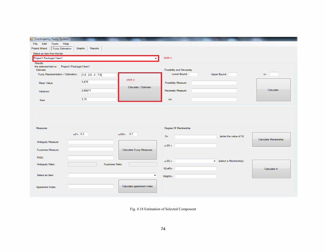
74
Fig. 4.18 Estimation of Selected Component

75
The measures sub category is used to calculate all the measures associated with selected
component. The additional input is the fuzziness weight and the ambiguity weight which
can be automatically generated. In case of non-acceptable input of the fuzziness weight
(i.e. bigger than 1) an error interactive screen will show up (Fig. 4.19):
𝑊𝐹 = 1 −𝑊𝐴𝐺 (4.1)
Fig. 4.19 Fuzziness Weight Input Error
The Ambiguity Measures (AG), Fuzziness Measures (F), Fuzziness Expected value Ratio
(FER), Ambiguity Expected value Ratio (AEV), and Fuzzy Number Quality Index
(FNQI) are calculated based on their equations. All the measures calculations can be done
by following 5 simple steps (Fig. 4.20) : 1) select a component from the first list, 2) enter
the fuzziness weight, 3) press the “Calculate Fuzzy Measures” button, 4) select another
component from the second drop-down list in order to calculate its agreement index, and
5) press the “Calculate Agreement Index” button.
The result of each measure will be shown in the correspondent field. This calculator
could be useful to check, monitor and control the contingency required for mitigating a
specific risk at any project milestone.

76
Fig. 4.20 Uncertainty Measures Calculations of a Selected Component
The possibility, necessity, and mλ uncertainty measures could be calculated based on their
equations 3.10, 3.11, and 3.12 respectively. The necessity, Possibility, and mλ measures
could be calculated by 5 steps (Fig. 4. 21): 1) select a component from the drop-down list,
2) enter the interval’s lower bound value, 3) enter the interval’s upper bound value, 4)
enter the λ value, and 5) press the “Calculate” button.

77
Fig. 4. 21 Possibility and Necessity Calculation of Selected Component
The Degree of Membership sub-category calculates the selected component’s degree of
membership for a given X and it calculates left and right value of X for a specific degree
of membership (Fig. 4. 22). The degree of membership calculations could be done as
follows: 1) select a component from the first list, 2) enter X value, 3) press “Calculate
Membership” button to calculate µ(X), 4) select membership desired value from µ(X)
drop-down list, and 5) press “Calculate X” button to calculate X (left) and X (right)
values.

78
Fig. 4. 22 Degree of Membership Calculations of Selected Component
4.2.4 Graphical Module
The graphical module generates a graphical representation of any project components
based on sub-components.
- Project could be represented by project, packages or by cost items.
- Package could be represented by package or cost items.
- Cost item could be represented by its fuzzy representation only.

79
The graphs can be drawn by three steps (Fig. 4. 23) as follows: 1) select component to be
represented, 2) select the desired representation’s option “By Project”, “By Package”, or
“By item”, and 3) press the “Plot” button
Fig. 4. 23 Graphical Representation of a Selected Component
4.2.5 Reporting Module
The reporting module is numerical output of CFSS organized in a table format. Each
component of the project has it fuzzy estimation, expected value, variance, uncertainty
measures, and contingency estimation. In addition to that, this report could be printed
directly from the software without the need to be converted to any other format (i.e.
Excel) with a print preview option as shown in (Fig. 4.24). The software output or project
report can be generated by following three steps as follows: 1) select the project from the
list, 2) press the “Generate Report” button, and 3) press the print / print preview report
button.

80
Fig. 4.24 Project Report
The report details can be modified to comply with the project or company requirements.
The software is coded by 100% vb.net including database, reporting, graphical
representation, fuzzy theory library, fuzzy operation and contingency estimation
procedures which afford the user great flexibility and options to customize and increase
the applicability to specific projects.
In Chapter 5 case studies and the data will be used to explicitly discuss and evaluate the
software and the proposed contingency estimating method. CFSS will be applied to two
real case studies extracted from literature in order to evaluate the software performance
and the efficiency of proposed estimating method compared to the existing methods
developed using fuzzy, MCS and PERT.
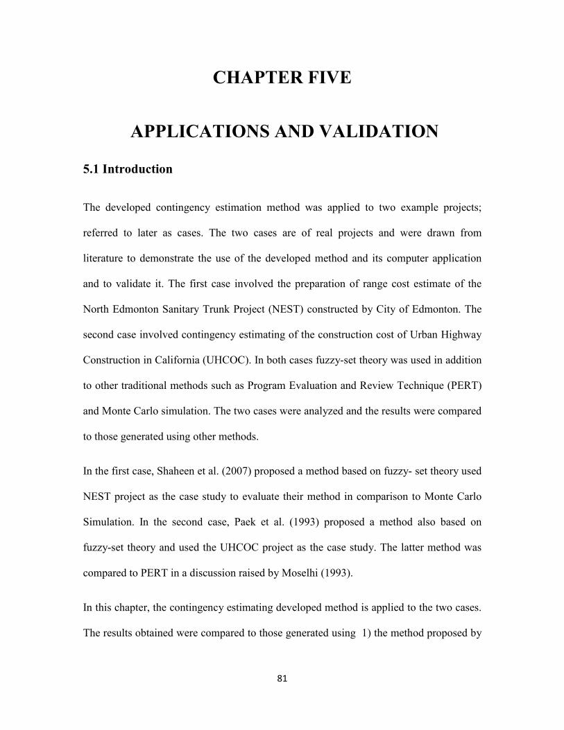
81
CHAPTER FIVE
APPLICATIONS AND VALIDATION
5.1 Introduction
The developed contingency estimation method was applied to two example projects;
referred to later as cases. The two cases are of real projects and were drawn from
literature to demonstrate the use of the developed method and its computer application
and to validate it. The first case involved the preparation of range cost estimate of the
North Edmonton Sanitary Trunk Project (NEST) constructed by City of Edmonton. The
second case involved contingency estimating of the construction cost of Urban Highway
Construction in California (UHCOC). In both cases fuzzy-set theory was used in addition
to other traditional methods such as Program Evaluation and Review Technique (PERT)
and Monte Carlo simulation. The two cases were analyzed and the results were compared
to those generated using other methods.
In the first case, Shaheen et al. (2007) proposed a method based on fuzzy- set theory used
NEST project as the case study to evaluate their method in comparison to Monte Carlo
Simulation. In the second case, Paek et al. (1993) proposed a method also based on
fuzzy-set theory and used the UHCOC project as the case study. The latter method was
compared to PERT in a discussion raised by Moselhi (1993).
In this chapter, the contingency estimating developed method is applied to the two cases.
The results obtained were compared to those generated using 1) the method proposed by

82
Paek et al. (1993), 2) the method proposed by Shaheen et al. (2007), 3) Monte Carlo
Simulation and 4) Program Evaluation and Review Technique (PERT).
5.2 Contingency and Range Estimating
As stated earlier, the proposed method was applied to the two case studies: 1) the North
Edmonton Sanitary Trunk (NEST) project (Shaheen et al., 2007), and 2) the UHCOC
project (Paek et al., 1993).
5.2.1 Case Study 1
The NEST project is a tunnelling project for the City of Edmonton called “North
Edmonton Sanitary Trunk”. The project had a maximum allocated budgeted of $8.8 M
and was estimated to cost $6 M. The main cost packages and their subcategories are
shown in Table 5. 1below.
Table 5. 1 Data of NEST Project Adopted with Shaheen et al. (2007)
Item # Description a b c d
1.1.1 Mobilization 40000 70000 70000 100000
1.1.2 Power Installation 89000 89000 89000 89000
1.1.3 Power – 156 Str. 15000 15000 50000 50000
1.2 Excavate Work shaft 97600 122000 122000 146400
1.3 Excavate Undercut 200000 269000 269000 350000
1.4 Excavate Tail Tunnel to East 100000 123000 123000 150000
1.5 Form and Pour Undercut 80000 80000 80000 80000

83
Item # Description a b c d
1.6 Form and Pour Tail Undercut 39000 39000 39000 39000
1.7 Form and Pour Shaft 100000 120000 120000 150000
2.1 Excavate Access Shaft 16000 16000 16000 16000
2.2
Backfill Shaft and Install
Segments 44000 44000 44000 44000
3.1
Tunnel Install Segments (866
m) price per m = 2254 $ 1951964 2142484 2142484 2909760
3.2 Patch and Rub Tunnel Crown 80 134 134 140
3.3
Patch and Rub
Tunnel Final Cleanup 161 188 188 215
3.4 Spoil Removal 5,4 8,1 8,1 9,7
4.1 Access Manhole Shaft 61000 61000 61000 61000
5.1
Tunnel and Install Segments
(756 m) price per m = 2254 $ 1704024 1870344 1870344 2540160
5.2 Patch and Rub Tunnel Crown 80 134 134 140
5.3
Patch and Rub Tunnel Final
Cleanup 161 188 188 215
5.4 Spoil Removal 5,4 8,1 8,1 9,7
6 Removal Shaft 101000 101000 101000 101000
The original data of each cost item was represented by a triangular fuzzy number that
maps the optimistic, most likely, and pessimistic estimates listed in Table 5. 1.

84
Subsequently, a unifying procedure was performed to modify each triangular fuzzy
number into a trapezoidal fuzzy number represented with quadruple (a, b, c, d). In
addition, the PERT formula was slightly modified in order to deal with quadruple fuzzy
number instead of its original triangular representation. The unified data is entered to the
input module of the developed software (CFSS) as shown in (Fig. 5. 1).
Fig. 5. 1 Data Input for NEST Project Case Study
The expected value (EV) of each cost item was then calculated; i.e. defuzzifief using
Equation 5.1:
𝐶𝑜𝑠𝑡 𝑖𝑡𝑒𝑚 (𝑅𝑖) = 𝐸𝑉(𝑅𝑖) (5.1)
The fuzzy cost-estimate at the package level (e.g. that of the main work shaft), which
contains several cost items was calculated as follows:

85
𝑓𝑢𝑧𝑧𝑦 𝑒𝑠𝑡𝑖𝑚𝑎𝑡𝑒 𝑜𝑓 𝑝𝑎𝑐𝑘𝑎𝑔𝑒(𝑃j) = � 𝑓𝑢𝑧𝑧𝑦 𝑒𝑠𝑡𝑖𝑚𝑎𝑡𝑒 𝑜𝑓 𝑐𝑜𝑠𝑡 𝑖𝑡𝑒𝑚(𝑅𝑖𝑗)𝑛
𝑖=1
(5.2)
The expected value of each package was calculated as follows:
𝐶𝑜𝑠𝑡 𝑝𝑎𝑐𝑘𝑎𝑔𝑒 (𝑃𝑗) = 𝐸𝑉(𝑃𝑗) (5.3)
And the fuzzy cost estimate of the project was calculated, accordingly as follows:
𝑇𝐶 = �𝑃𝑗𝑚
𝑗=1
(5.4)
Then; the project cost value was calculated by defuzzifiying TC in Equation 5.4 above as:
𝐸𝑠𝑡𝑖𝑚𝑎𝑡𝑒𝑑 𝑝𝑟𝑜𝑗𝑒𝑐𝑡 𝐶𝑜𝑠𝑡 (𝐶) = 𝐸𝑉(𝑇𝐶) (5.5)
Once all the calculated estimates of cost items, packages, and project were completed, a
full report was then generated as shown in (Fig. 5. 2). This report provides not only the
expected value of project cost, but also a number of measures, indices and the depict the
level of the uncertainty associated with project cost; representing the vagueness and
imprecision implicit in the estimated cost.
• The fuzzy estimate calculated for the NEST project using the proposed method is:
[4,639,030; 5,162,160; 5,197,160; 6,827,140].
• The above fuzzy estimate, being in the form of a trapezoidal fuzzy number, its
expected value was calculated by defuzzifiying it as described in Chapter 3. This
yielded project expected cost value of $ 5, 456, 373 M.
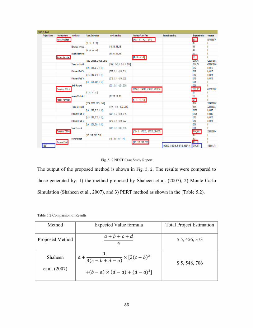
86
Fig. 5. 2 NEST Case Study Report
The output of the proposed method is shown in Fig. 5. 2. The results were compared to
those generated by: 1) the method proposed by Shaheen et al. (2007), 2) Monte Carlo
Simulation (Shaheen et al., 2007), and 3) PERT method as shown in the (Table 5.2).
Table 5.2 Comparison of Results
Method Expected Value formula Total Project Estimation
Proposed Method 𝑎 + 𝑏 + 𝑐 + 𝑑4
$ 5, 456, 373
Shaheen
et al. (2007)
𝑎 +1
3(𝑐 − 𝑏 + 𝑑 − 𝑎) × [2(𝑐 − 𝑏)2
+(𝑏 − 𝑎) × (𝑑 − 𝑎) + (𝑑 − 𝑎)²]
$ 5, 548, 706
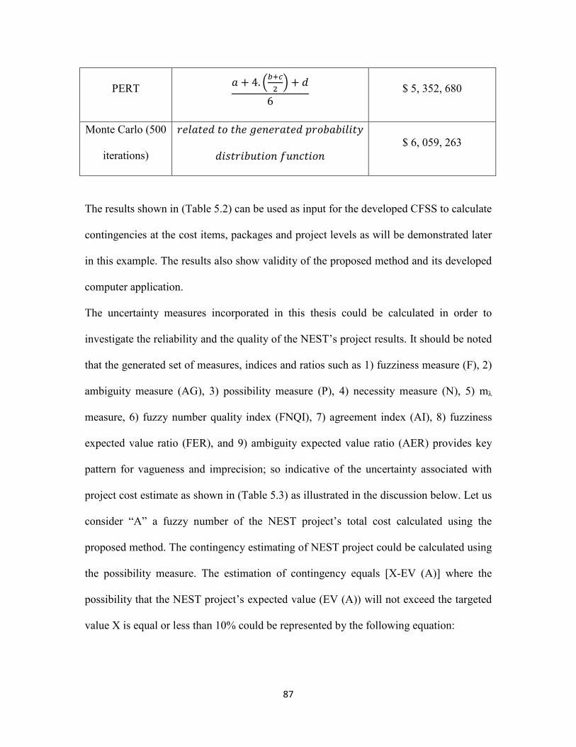
87
PERT 𝑎 + 4. �𝑏+𝑐2� + 𝑑
6 $ 5, 352, 680
Monte Carlo (500
iterations)
𝑟𝑒𝑙𝑎𝑡𝑒𝑑 𝑡𝑜 𝑡ℎ𝑒 𝑔𝑒𝑛𝑒𝑟𝑎𝑡𝑒𝑑 𝑝𝑟𝑜𝑏𝑎𝑏𝑖𝑙𝑖𝑡𝑦
𝑑𝑖𝑠𝑡𝑟𝑖𝑏𝑢𝑡𝑖𝑜𝑛 𝑓𝑢𝑛𝑐𝑡𝑖𝑜𝑛 $ 6, 059, 263
The results shown in (Table 5.2) can be used as input for the developed CFSS to calculate
contingencies at the cost items, packages and project levels as will be demonstrated later
in this example. The results also show validity of the proposed method and its developed
computer application.
The uncertainty measures incorporated in this thesis could be calculated in order to
investigate the reliability and the quality of the NEST’s project results. It should be noted
that the generated set of measures, indices and ratios such as 1) fuzziness measure (F), 2)
ambiguity measure (AG), 3) possibility measure (P), 4) necessity measure (N), 5) mλ
measure, 6) fuzzy number quality index (FNQI), 7) agreement index (AI), 8) fuzziness
expected value ratio (FER), and 9) ambiguity expected value ratio (AER) provides key
pattern for vagueness and imprecision; so indicative of the uncertainty associated with
project cost estimate as shown in (Table 5.3) as illustrated in the discussion below. Let us
consider “A” a fuzzy number of the NEST project’s total cost calculated using the
proposed method. The contingency estimating of NEST project could be calculated using
the possibility measure. The estimation of contingency equals [X-EV (A)] where the
possibility that the NEST project’s expected value (EV (A)) will not exceed the targeted
value X is equal or less than 10% could be represented by the following equation:
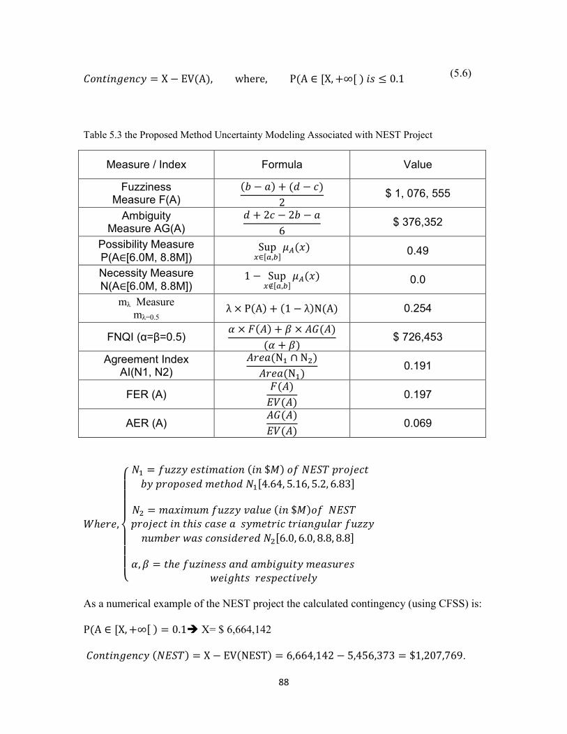
88
𝐶𝑜𝑛𝑡𝑖𝑛𝑔𝑒𝑛𝑐𝑦 = X − EV(A), where, P(A ∈ [X, +∞[ ) 𝑖𝑠 ≤ 0.1 (5.6)
Table 5.3 the Proposed Method Uncertainty Modeling Associated with NEST Project
Measure / Index Formula Value
Fuzziness Measure F(A)
(𝑏 − 𝑎) + (𝑑 − 𝑐)2
$ 1, 076, 555
Ambiguity Measure AG(A)
𝑑 + 2𝑐 − 2𝑏 − 𝑎6
$ 376,352
Possibility Measure P(A∈[6.0M, 8.8M])
Sup𝑥∈[𝑎,𝑏]
𝜇𝐴(𝑥) 0.49
Necessity Measure N(A∈[6.0M, 8.8M])
1 − Sup𝑥∉[𝑎,𝑏]
𝜇𝐴(𝑥) 0.0
mλ Measure mλ=0.5
λ × P(A) + (1 − λ)N(A) 0.254
FNQI (α=β=0.5) 𝛼 × 𝐹(𝐴) + 𝛽 × 𝐴𝐺(𝐴)
(𝛼 + 𝛽) $ 726,453
Agreement Index AI(N1, N2)
𝐴𝑟𝑒𝑎(N1 ∩ N2)𝐴𝑟𝑒𝑎(N1)
0.191
FER (A) 𝐹(𝐴)𝐸𝑉(𝐴)
0.197
AER (A) 𝐴𝐺(𝐴)𝐸𝑉(𝐴)
0.069
𝑊ℎ𝑒𝑟𝑒,
⎩⎪⎪⎪⎨
⎪⎪⎪⎧𝑁1 = 𝑓𝑢𝑧𝑧𝑦 𝑒𝑠𝑡𝑖𝑚𝑎𝑡𝑖𝑜𝑛 (𝑖𝑛 $𝑀) 𝑜𝑓 𝑁𝐸𝑆𝑇 𝑝𝑟𝑜𝑗𝑒𝑐𝑡 𝑏𝑦 𝑝𝑟𝑜𝑝𝑜𝑠𝑒𝑑 𝑚𝑒𝑡ℎ𝑜𝑑 𝑁1[4.64, 5.16, 5.2, 6.83]
𝑁2 = 𝑚𝑎𝑥𝑖𝑚𝑢𝑚 𝑓𝑢𝑧𝑧𝑦 𝑣𝑎𝑙𝑢𝑒 (𝑖𝑛 $𝑀)𝑜𝑓 𝑁𝐸𝑆𝑇
𝑝𝑟𝑜𝑗𝑒𝑐𝑡 𝑖𝑛 𝑡ℎ𝑖𝑠 𝑐𝑎𝑠𝑒 𝑎 𝑠𝑦𝑚𝑒𝑡𝑟𝑖𝑐 𝑡𝑟𝑖𝑎𝑛𝑔𝑢𝑙𝑎𝑟 𝑓𝑢𝑧𝑧𝑦 𝑛𝑢𝑚𝑏𝑒𝑟 𝑤𝑎𝑠 𝑐𝑜𝑛𝑠𝑖𝑑𝑒𝑟𝑒𝑑 𝑁2[6.0, 6.0, 8.8, 8.8]
𝛼,𝛽 = 𝑡ℎ𝑒 𝑓𝑢𝑧𝑖𝑛𝑒𝑠𝑠 𝑎𝑛𝑑 𝑎𝑚𝑏𝑖𝑔𝑢𝑖𝑡𝑦 𝑚𝑒𝑎𝑠𝑢𝑟𝑒𝑠
𝑤𝑒𝑖𝑔ℎ𝑡𝑠 𝑟𝑒𝑠𝑝𝑒𝑐𝑡𝑖𝑣𝑒𝑙𝑦
As a numerical example of the NEST project the calculated contingency (using CFSS) is:
P(A ∈ [X, +∞[ ) = 0.1 X= $ 6,664,142
𝐶𝑜𝑛𝑡𝑖𝑛𝑔𝑒𝑛𝑐𝑦 (𝑁𝐸𝑆𝑇) = X − EV(NEST) = 6,664,142 − 5,456,373 = $1,207,769.
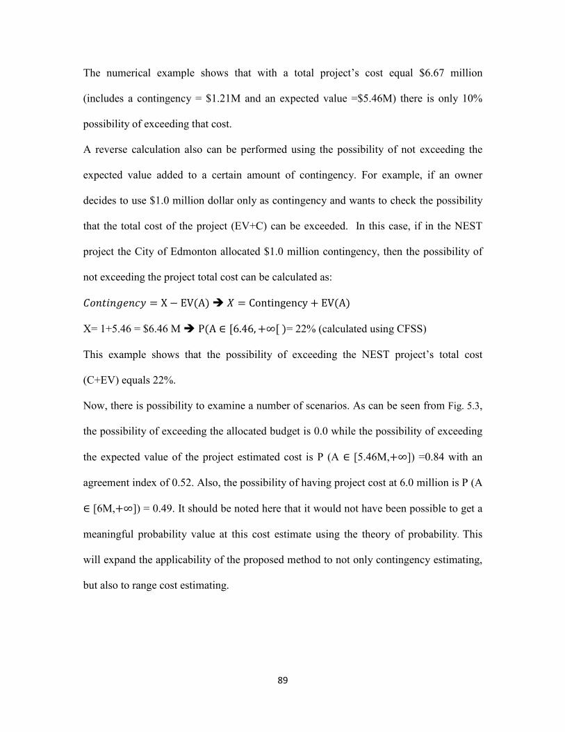
89
The numerical example shows that with a total project’s cost equal $6.67 million
(includes a contingency = $1.21M and an expected value =$5.46M) there is only 10%
possibility of exceeding that cost.
A reverse calculation also can be performed using the possibility of not exceeding the
expected value added to a certain amount of contingency. For example, if an owner
decides to use $1.0 million dollar only as contingency and wants to check the possibility
that the total cost of the project (EV+C) can be exceeded. In this case, if in the NEST
project the City of Edmonton allocated $1.0 million contingency, then the possibility of
not exceeding the project total cost can be calculated as:
𝐶𝑜𝑛𝑡𝑖𝑛𝑔𝑒𝑛𝑐𝑦 = X − EV(A) 𝑋 = Contingency + EV(A)
X= 1+5.46 = $6.46 M P(A ∈ [6.46, +∞[ )= 22% (calculated using CFSS)
This example shows that the possibility of exceeding the NEST project’s total cost
(C+EV) equals 22%.
Now, there is possibility to examine a number of scenarios. As can be seen from Fig. 5.3,
the possibility of exceeding the allocated budget is 0.0 while the possibility of exceeding
the expected value of the project estimated cost is P (A ∈ [5.46M,+∞]) =0.84 with an
agreement index of 0.52. Also, the possibility of having project cost at 6.0 million is P (A
∈ [6M,+∞]) = 0.49. It should be noted here that it would not have been possible to get a
meaningful probability value at this cost estimate using the theory of probability. This
will expand the applicability of the proposed method to not only contingency estimating,
but also to range cost estimating.
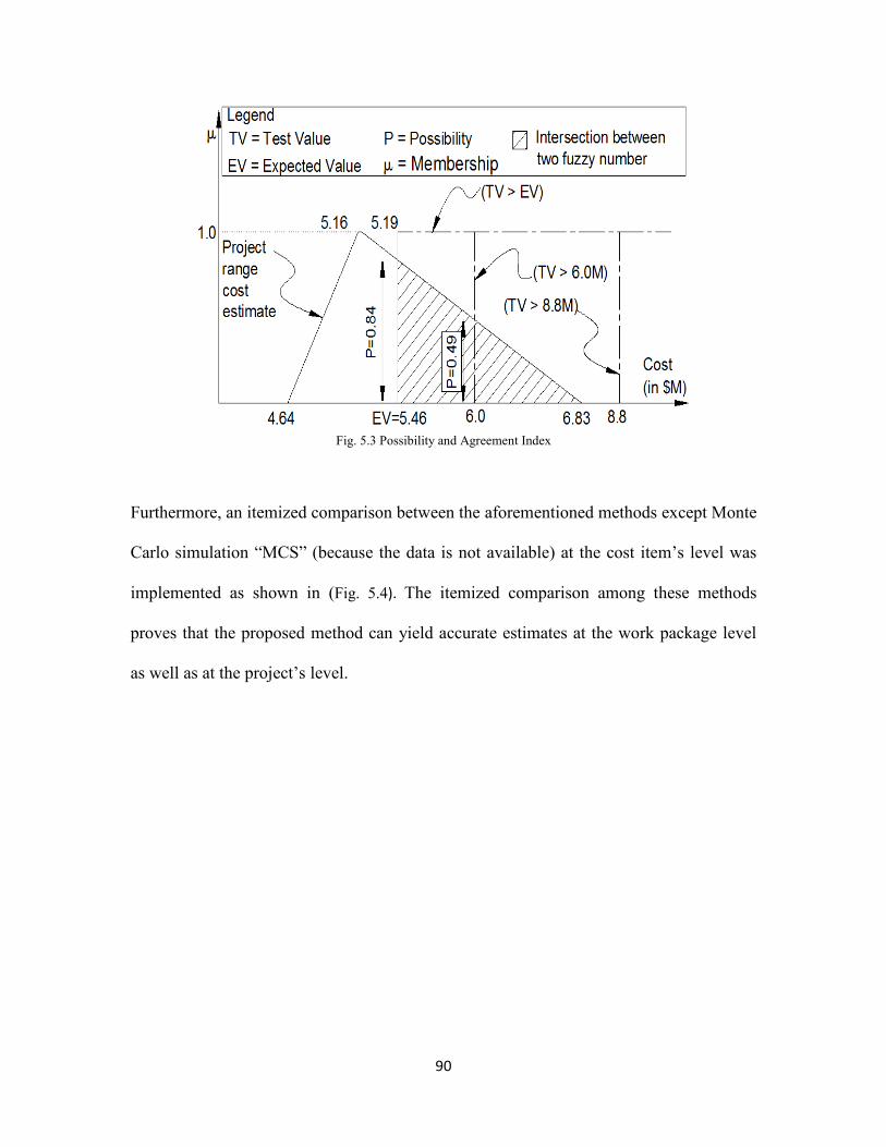
90
Fig. 5.3 Possibility and Agreement Index
Furthermore, an itemized comparison between the aforementioned methods except Monte
Carlo simulation “MCS” (because the data is not available) at the cost item’s level was
implemented as shown in (Fig. 5.4). The itemized comparison among these methods
proves that the proposed method can yield accurate estimates at the work package level
as well as at the project’s level.

91
Fig. 5.4 Itemized Comparison among Proposed Method, PERT and Shaheen Method
5.2.2 Case Study 2
Paek et al. (1993) used the project of an urban highway construction in California as the
case study. In this research the project is referred to as the UHCOC project. The UHCOC
project was projected to cost $800 million. The risk plan associated with this project
treats both positive risks (threats) and negative risks (opportunity). The cost data of this
project is summarized in Table 5. 4 and Table 5. 5. For unifying the data in order to
comply with the automated computer application’s input format the following operations
were applied:
700008900020833,33333
122000
271000
123666,666780000
39000121666,6667
1600044000
2238610
126 188 7,91666666761000
1954260
126 188 7,916666667
101000700008900032500
122000
272000
12400080000
39000122500
1600044000
2286673
122 188 7,82561000
1996218
122 188 7,825
101000700008900032500
122000
273000
124333,333380000
39000123333,3333
1600044000
2334736
118 188 7,73333333361000
2038176
118 188 7,733333333
101000
0
500000
1000000
1500000
2000000
2500000
0 5 10 15 20 25
COST
($)
ITEM NUMBER
PROPOSED METHOD VS. PERT AND SHAHEEN METHOD
PERT
SALAH
SHAHEEN

92
1. Converting the most likely range [a, b] to the “b” and “c” elements of the fuzzy
number’s quadruple (a, b, c, d).
2. Converting the largest likely range [c, d] to the “a” and “d” elements of the fuzzy
number’s quadruple (a, b, c, d).
3. Modifying the negative risks’ contingency values to negative fuzzy numbers’
quadruples (-d, -c, -b, -a) instead of (a, b, c, d).
The above modifications are important to unify data input of the methods used for
comparison. The positive risks data or threats (after modification) are illustrated in (Table
5. 4). The positives risks are classified into two types: 1) risks associated with estimation,
and 2) risks not associated with estimation.
Table 5. 4 UHCOC Positive Risks Data Input
Positive risk elements a b c d
Estimation Risks
Topsoil quantity overrun – 150,000 cu. Yd. 255 285 315 345
Additional retaining walls and pilings under retaining walls 3500 4500 5250 5500
Additional wick-drain pipe 120 142 150 150
Additional remedial excavation in lieu of wick-drain pipe 1400 1800 2000 2400
Rock quantity overrun – drill and shoot by 25% 2550 3230 3570 4250
Additional 1-mi hauling distance of drill and shoot rock 2000 2375 2625 3000
Disposal fee $1.0 / cu. Yd for drill and shoot rock 4165 4753 5047 5635
Increase in all storm drainage pipe by 6 in. 1040 1170 1430 1560
Increase in reinforced concrete pipe quantity by 15% 1360 1615 1700 1700
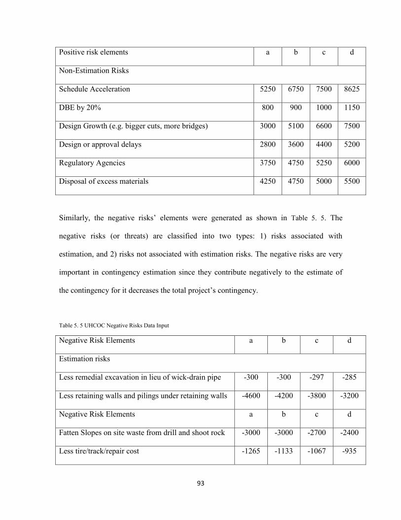
93
Positive risk elements a b c d
Non-Estimation Risks
Schedule Acceleration 5250 6750 7500 8625
DBE by 20% 800 900 1000 1150
Design Growth (e.g. bigger cuts, more bridges) 3000 5100 6600 7500
Design or approval delays 2800 3600 4400 5200
Regulatory Agencies 3750 4750 5250 6000
Disposal of excess materials 4250 4750 5000 5500
Similarly, the negative risks’ elements were generated as shown in Table 5. 5. The
negative risks (or threats) are classified into two types: 1) risks associated with
estimation, and 2) risks not associated with estimation risks. The negative risks are very
important in contingency estimation since they contribute negatively to the estimate of
the contingency for it decreases the total project’s contingency.
Table 5. 5 UHCOC Negative Risks Data Input
Negative Risk Elements a b c d
Estimation risks
Less remedial excavation in lieu of wick-drain pipe -300 -300 -297 -285
Less retaining walls and pilings under retaining walls -4600 -4200 -3800 -3200
Negative Risk Elements a b c d
Fatten Slopes on site waste from drill and shoot rock -3000 -3000 -2700 -2400
Less tire/track/repair cost -1265 -1133 -1067 -935
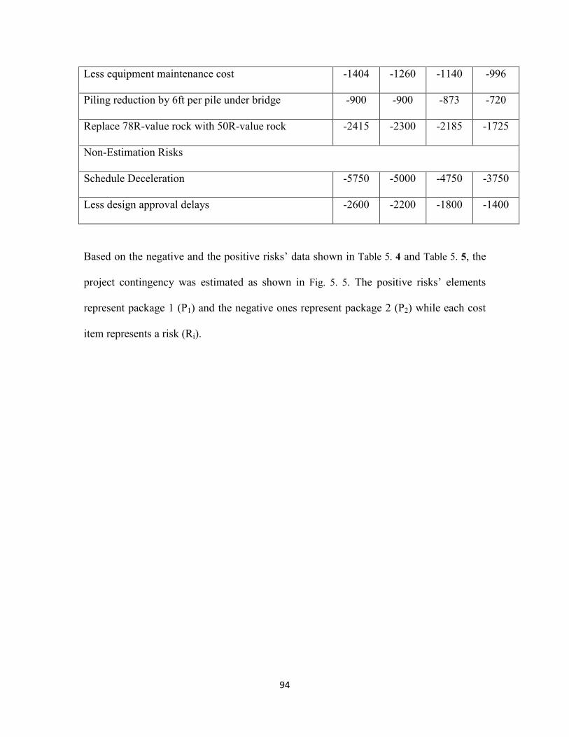
94
Less equipment maintenance cost -1404 -1260 -1140 -996
Piling reduction by 6ft per pile under bridge -900 -900 -873 -720
Replace 78R-value rock with 50R-value rock -2415 -2300 -2185 -1725
Non-Estimation Risks
Schedule Deceleration -5750 -5000 -4750 -3750
Less design approval delays -2600 -2200 -1800 -1400
Based on the negative and the positive risks’ data shown in Table 5. 4 and Table 5. 5, the
project contingency was estimated as shown in Fig. 5. 5. The positive risks’ elements
represent package 1 (P1) and the negative ones represent package 2 (P2) while each cost
item represents a risk (Ri).
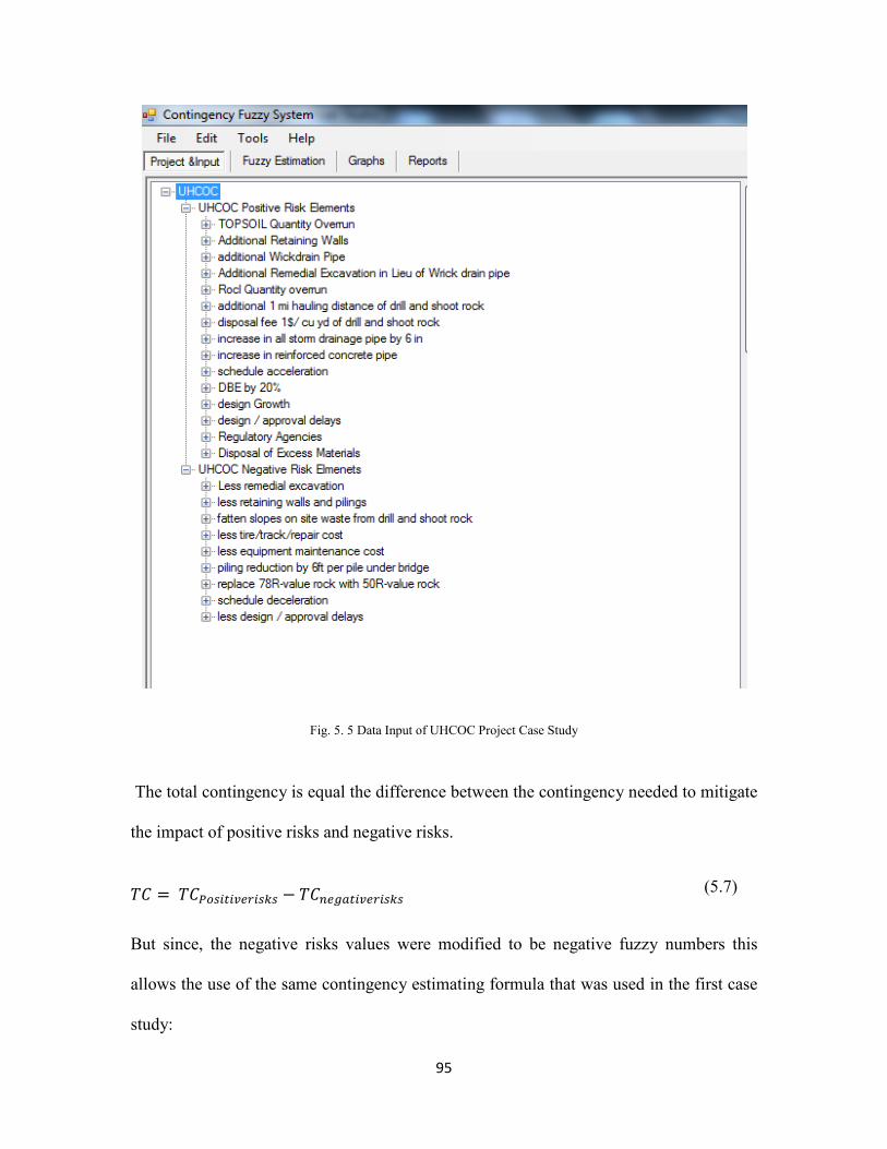
95
Fig. 5. 5 Data Input of UHCOC Project Case Study
The total contingency is equal the difference between the contingency needed to mitigate
the impact of positive risks and negative risks.
𝑇𝐶 = 𝑇𝐶𝑃𝑜𝑠𝑖𝑡𝑖𝑣𝑒𝑟𝑖𝑠𝑘𝑠 − 𝑇𝐶𝑛𝑒𝑔𝑎𝑡𝑖𝑣𝑒𝑟𝑖𝑠𝑘𝑠 (5.7)
But since, the negative risks values were modified to be negative fuzzy numbers this
allows the use of the same contingency estimating formula that was used in the first case
study:
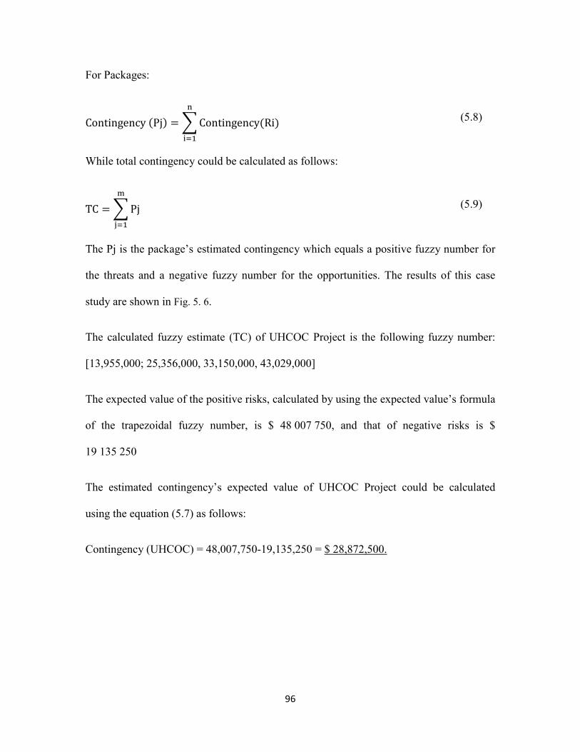
96
For Packages:
Contingency (Pj) = �Contingency(Ri)n
i=1
(5.8)
While total contingency could be calculated as follows:
TC = �Pjm
j=1
(5.9)
The Pj is the package’s estimated contingency which equals a positive fuzzy number for
the threats and a negative fuzzy number for the opportunities. The results of this case
study are shown in Fig. 5. 6.
The calculated fuzzy estimate (TC) of UHCOC Project is the following fuzzy number:
[13,955,000; 25,356,000, 33,150,000, 43,029,000]
The expected value of the positive risks, calculated by using the expected value’s formula
of the trapezoidal fuzzy number, is $ 48 007 750, and that of negative risks is $
19 135 250
The estimated contingency’s expected value of UHCOC Project could be calculated
using the equation (5.7) as follows:
Contingency (UHCOC) = 48,007,750-19,135,250 = $ 28,872,500.

97
Fig. 5. 6 UHCOC Case Study Report
The output summary of proposed method, PERT, and the method proposed by Paek
(1993) is shown in Table 5. 6.
Table 5. 6 Comparison of Results (Case 2)
Method Expected Value Formula Total Project Estimation
Proposed Method a + b + c + d4
$ 28, 872, 500
Paek (1993) V1 + V2
2(W1 + W2) $ 28, 968, 350
PERT (Moselhi,1993) a + 4. �b+c2�+ d
6 $ 29, 292, 000
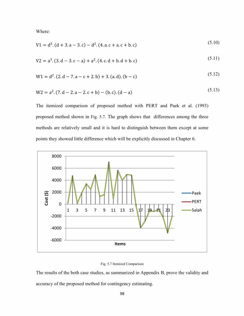
98
Where:
V1 = d3. (d + 3. a − 3. c) − d2. (4. a. c + a. c + b. c) (5.10)
V2 = a3. (3. d − 3. c − a) + a2. (4. c. d + b. d + b. c) (5.11)
W1 = d2. (2. d − 7. a − c + 2. b) + 3. (a. d). (b − c) (5.12)
W2 = a2. (7. d − 2. a − 2. c + b) − (b. c). (d − a) (5.13)
The itemized comparison of proposed method with PERT and Paek et al. (1993)
proposed method shown in Fig. 5.7. The graph shows that differences among the three
methods are relatively small and it is hard to distinguish between them except at some
points they showed little difference which will be explicitly discussed in Chapter 6.
Fig. 5.7 Itemized Comparison
The results of the both case studies, as summarized in Appendix B, prove the validity and
accuracy of the proposed method for contingency estimating.
-6000
-4000
-2000
0
2000
4000
6000
8000
1 3 5 7 9 11 13 15 17 19 21 23
Cost
($)
Items
Paek
PERT
Salah
99
For the contingency management, two case studies on depletion of contingency over
project durations were analyzed in the literature review chapter supports the developed
contingency management method on two fronts; 1) the inclusion of different depletion
models, as well as, 2) the factors used in chapter three to provide the decision support for
the selection of most suitable depletion curve.
In Chapter 6, the results of the contingency estimating and management obtained based
on the proposed method are highlighted along with the advantages and limitations of the
method.
100
CHAPTER SIX
RESULTS DISCUSSION
6.1 Introduction
Project managers are usually opposed to the introduction of new applications and tools.
Typically the old “tired and true” methodology is more comfortable because of reasons
such as: 1) complexity of new method, 2) time or resources consuming, difficulty to
verify and the need for an experienced to apply the method. The proposed contingency
estimating method was designed with the end user in mind. The proposed method is easy
to use while still remaining: 1) accurate, 2) fast, 3) verifiable, and 4) applicable without
the historical data records. In addition, the coded user-friendly tool generates dual
analytical and graphical outputs that support the project managers’ decision making.
Furthermore, the proposed contingency management method gives a wide range of
possibilities to deplete contingency with any convenient strategy (aggressive or passive)
based on the project manager skills and company’s policy. The tailored depletion (custom
depletion) curve increases the of project managers control over depleted contingency
compared to the estimated contingency at any milestone. This comparison provides
significant information about contingency depletion performance.
In this chapter, the results of the selected case studies will be discussed and a comparison,
based on the relative error, between the proposed contingency estimating’s method and
other methods will be presented. Furthermore, the limitations of the proposed method,
advantages, and disadvantages over the other methods will be identified. Also, the
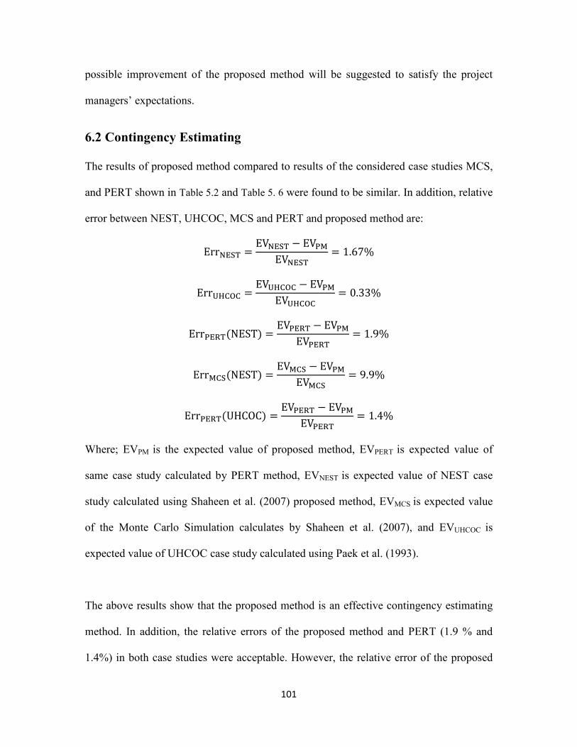
101
possible improvement of the proposed method will be suggested to satisfy the project
managers’ expectations.
6.2 Contingency Estimating
The results of proposed method compared to results of the considered case studies MCS,
and PERT shown in Table 5.2 and Table 5. 6 were found to be similar. In addition, relative
error between NEST, UHCOC, MCS and PERT and proposed method are:
ErrNEST =EVNEST − EVPM
EVNEST= 1.67%
ErrUHCOC =EVUHCOC − EVPM
EVUHCOC= 0.33%
ErrPERT(NEST) =EVPERT − EVPM
EVPERT= 1.9%
ErrMCS(NEST) =EVMCS − EVPM
EVMCS= 9.9%
ErrPERT(UHCOC) =EVPERT − EVPM
EVPERT= 1.4%
Where; EVPM is the expected value of proposed method, EVPERT is expected value of
same case study calculated by PERT method, EVNEST is expected value of NEST case
study calculated using Shaheen et al. (2007) proposed method, EVMCS is expected value
of the Monte Carlo Simulation calculates by Shaheen et al. (2007), and EVUHCOC is
expected value of UHCOC case study calculated using Paek et al. (1993).
The above results show that the proposed method is an effective contingency estimating
method. In addition, the relative errors of the proposed method and PERT (1.9 % and
1.4%) in both case studies were acceptable. However, the relative error of the proposed

102
method and Monte Carlo Simulation (500 iterations) is relatively high (9.9%) but still
within the acceptable range (<10%). This indicates the accuracy and indicates usefulness
of the proposed method.
The advantages introduced in this discussion prove that the proposed method is:
• Accurate compared to other methods.
• Simple, given it has no complicated calculations involved and it is supported by a
user-friendly computer aided tool which eliminates the need to an experienced user.
• Supportive and informative method, since it offers a set of indices and measures that
address vagueness and imprecision associated with estimated cost at the cost item,
work package and project levels, as well as possibility of having project cost at a
specific crisp value or within a specified cost range.
• Need-less resources, since it doesn’t require historical data records to construct
probability density functions for the cost items involved and it doesn’t require large
simulation.
• Direct and flexible. Since it offers multiple options to introduce convenient estimation
based on expert’s experience without any restriction on the input shape (i.e. the expert
can use null, crisp, uniform, triangular, and trapezoidal fuzzy number). This
eliminates the expert’s subjectivity and his gut-feel estimation.
The disadvantages are limited since all the disadvantages are related to the proposed
method’s assumptions:
• Assumption 1: This assumption was considered for the automated tool that coded
using VB.NET. This tool assumed three levels (item, package, and cost) of Risk

103
Break down Structure only. In reality, this can be insufficient for a mega project
that may include several packages, sub-packages, and multi-level risks.
• Assumption 2: All risks associated with investigated project assumed to be
identified; however the unknown risks cannot be estimated because it will be
identified just when they happen.
• Assumption 3: the proposed method assumed that risk is represented by one of the
four types of fuzzy numbers. However, the membership of a fuzzy number can
have any shape.
Based on the aforementioned assumptions, the proposed method is able to: 1) deal with
identified risks only, 2) incorporate limited types of fuzzy representation, and 3) consider
three levels of risk breakdown structure only.
6.3 Contingency Management
The proposed method for contingency management was generated from current practice.
Usually, the company’s experience and the learned lessons from similar projects in the
past generate the company’s practice in contingency management. The contingency
depletion procedure currently followed by companies is governed by several factors such
as: 1) project manager’s strategy (i.e. passive or aggressive), 2) the project type and
complexity (i.e. infrastructure, airport), 3) the project delivery system and contract type
(i.e. traditional, fast track, GMP), and 4) the company’s financial capacity.
The factors affected the contingency management and depletion, were considered in the
proposed method. In addition, the proposed tailored depletion (custom depletion) curve is
a new procedure to deplete, manage, and control the project contingency. This procedure

104
presents an effective and comparative tool of depleted contingency versus estimated
contingency and gives ability to monitor and control them at any contingency milestone.
However, the proposed depletion curves have different advantages and disadvantages
based on different factors. Therefore, a flexible selection procedure, based on the IF-
AND-THEN approach, was proposed. The selection procedure changed based on the
aforementioned factors affecting the contingency depletion.
It is noted that actual depletion curve is also associated with unknown risks which may
occur over project durations. The occurrence of unknown risks or unforeseen risks may
affect the shape of depletion curve un-predictably.
The flexibility of the proposed method and selection procedure can overcome the current
practice’s limitations or assumptions. This procedure is based on the project
characteristics and the actual factors affecting project’s contingency depletion such as : 1)
the available information (i.e. project type, details, risks type, financial capacity, learned
lessons and experience etc…), and 2) the project manager’s preferred strategy in
contingency depletion (i.e. passive or aggressive).
The subjectivity involved in decision making of a contingency depletion curve selection
can be considered as a limitation since it is related to the reliability and availability of
information. Otherwise, it is a useful and supportive methodology since it increases
ability the ability of project manager to check contingency depletion performance at any
milestone as shown the selected case studies.
Finally, the proposed method for contingency management can be followed and applied
instead of the current practices. The proposed method decreases the decision making
105
subjectivity, eliminates the trial and error intentions, and offers an effective selection
procedure based on reliable information (i.e. company’s past experience and learned
lessons).
The chapter 7 includes: 1) summary of this research contributions, 2) conclusions about
the proposed methods, 3) few future research recommendations.

106
CHAPTER SEVEN
CONCLUSIONS AND RECOMMENDATIONS
7.1 Summary
This study presents a contingency estimating method based on fuzzy set theory. The
methodology encompasses three major fronts; 1) assessment of contingency which
represents the cost items associated with the project by fuzzy numbers based on experts’
judgement, 2) application of fuzzy set theory on input in order to calculate the fuzzy
representation at cost item, package, and project levels, and 3) defuzzification of the
calculated fuzzy numbers using one of the defuzzification methodologies (i.e. center of
area) in order to estimate the contingencies represented by these fuzzy numbers.
As well, an automated computer application called Contingency Fuzzy System Software
(CFSS) was developed. CFSS was coded using VB.net to automate the application of the
developed method. The developed software allows contingency estimators and the
contingency managers to evaluate and monitor contingency at the work package and
project levels. The outputs reports generated by the CFSS are detailed and informative
which increases the project manager’s ability to address the contingency analytically and
graphically using a wide range of scenarios pertinent to contingency estimating and
management over project duration.
New contingency management methodology is introduced; based on “tailored/custom
depletion” curve and the depletion curve selection procedure. The depletion baseline
107
improves contingency management efficiency and facilitates its monitoring and
controlling over project durations. The methodology allows for the utilization of five
different types of depletion curves: 1) Linear, 2) Basic/S-Curve, 3) Back-End Loading, 4)
Front-End Loading, 5) Tailored or custom. The first four curves are identified from the
subjective practice of the project managers and companies based on their past experience.
The selection procedure, using the IF-AND-THEN type approach, is introduced based on
several factors such as; project type, project manager strategy, company financial
support, risk impact, and severity as well as rate of occurrence. Actual case studies were
analyzed to demonstrate the accuracy and usefulness of the proposed method for
contingency estimating. Two case studies drawn from literature were analysed in order to
support the decision for the selection of the most suitable depletion curve. The case
studies results were discussed based on comparison among the proposed methods and
those commonly used in literature. In this chapter, contributions of this research,
conclusions, and some recommendations for future research will be presented.
7.2 Research Contributions
The contributions made in this research consist of a comprehensive study of contingency
estimating and management method and the development of contingency estimating and
management methods. The development made in this research includes:
• New method for contingency estimating based on fuzzy set theory
• Automated software used to estimate, monitor and control contingency at the
work package and project levels.
108
• New method for contingency management based on risk-driven contingency
depletion over project durations.
• Depletion curve selection procedure based on a set of impact factors and the use
of IF-AND-THEN type approach.
• Documentation of current practice in contingency management based on company
policies, project manager’s experience, and management skills.
7.3 Conclusion
In this thesis, estimating contingency using fuzzy set theory was proven to be effective
and does not require large data as in the case of computer simulation. the results obtained
using the developed method are comparable to those generated by other methods such as:
1) PERT, 2) the method of Shaheen et al. (2007) , 3) the method of Paek et al. (1993),
and 4) Monte Carlo Simulation. The use of fuzzy set theory has an advantage of
providing easier, faster, and reliable output, with the capacity to examine a wide range of
scenarios; some cannot be considered using any probability-based method. The collection
of data from experts using proposed procedure will encourage them to express their
knowledge using different formats (e.g. crisp fuzzy number, triangular fuzzy number).
The analysed case studies (NEST and UHCOC) along with their results confirmed
validity and accuracy of the proposed contingency estimating method.
Similarly for the contingency management, the analyzed case studies proved usefulness
of the proposed method for contingency management and its depletion over project
durations. The proposed method helps to establish a systematic methodology for

109
contingency depletion, based on the depletion curves extracted from the common practice
and the consideration of past experience of the organizations involved.
The depletion curve selection procedure also is flexible in selecting suitable planned
depletion curve for projects based on several risk-driven impact factors. The proposed
selection approach (IF-AND-THEN) combines project factors, management skill factors,
risk factors, and company factors (e.g. financial capacity) in search of reasonable, logical,
and systematic contingency depletion curve selection.
7.4 Future Work
Based on the subjects’ richness and the needs associated with contingency management
and estimating subjects, the following is recommended for future work:
1) Improving contingency estimation automated tool by implementing multi-level risk
activities with multi-level of risk breakdown structure (e.g. more than three);
2) Methods generalization could be done by considering additional fuzzy number shapes
with different membership functions; and
3) The contingency estimating method can be re-compared to the Monte Carlo
Simulation with different probability density function and number of iterations.
This work is certain to become the basis for a considerable number of valuable research
studies.
4) The developed contingency management method can be applied to a real project to
measure its effectiveness.
110
REFERENCES
American Association of Civil Engineers, (2007),"Cost Engineering Terminology", AACE International, Recommended Practice 10S-90, rev. 2007 Abdelgawad, M., Robinson, A., Martinez, F., (2010), "Quantitative Assessment of Horizontal Directional Drilling Project Risk Using Fuzzy Fault Tree Analysis”, ASCE-Construction Research Congress, pp. 1274-1283
Amaya, A. J. R., Lengerke, O., Cosenza, C., Dutra, M. S., and Tavera, M. J. M. (2009), "Comparison of Defuzzification Methods: Automatic Control of Temperature and Flow in Heat Exchanger", Automation and Control, pp. 77-88
Ang, A.H., and Tang, W.H. (1975), "Probability Concepts in Engineering Planning and Design", Basic Principles, Vol. 1
Baccarini, D. (2006), "The Maturing Concept of Estimating Project Cost Contingency", Educators Association Conference
Baccarini, D., and Archer, R. (2001), "The Risk Ranking of Project: a Methodology", International Journal of Project Management, Vol. 19, pp. 139-145
Barraza, G., and Bueno, R. (2007), "Cost Contingency Management", Journal of Construction Engineering and Management, Vol. 23, No. 3, pp.140-146
Barraza, G. (2011) "Probabilistic Estimation and Allocation of Project Time Contingency”, Journal of Construction Engineering and Management, Vol. 137, No. 4, pp. 259-265
Carlsson, C., Fedrizzi, M., and Fuller, R. (2004), "Fuzzy Logic in Management", Kluwer Academic Publishers
Chen, D., and Hartman, F. T. (2000), "A Neural Network Approach to Risk Assessment and Contingency Allocation". AACE Transactions, 24-27th June, Risk.07.01-6
City of Jonesobro, (2004), “Transmission / Substation Projects”, Entergy Arkansas Jonesboro, 04-046-U
Colville, R. (2008), “Considerations in Project Cost Estimation”, Baxter Business Services Delgado, M., Vila, M. A., and Woxman, W. (1998), "On a Canonical Representation of Fuzzy Numbers", fuzzy set system, Vol. 93, No. 1, pp. 125-135

111
Department of Transportation- CANADA (2009), Contingencies and Supplemental Work Approval Procedure”, Federal Highway Association (FHWA), PDD09-4, Appendix A - attachment “F”
Diekmann, J. E., Sewester, E. E., and Taher, K. (1988), ‘‘Risk Management in Capital Projects’’, Construction Industry Institute
Dorp, J. R., and Kotz, S. (2003), "Generalized Trapezoidal Distribution", Metrika, Vol. 58, No. 1, pp. 85-97
Dubois, D., Foulloy, L., Mauris, G., and Prade, H. (2004), "Probability- Possibility Transformations, Triangular Fuzzy Sets, and Probabilistic Inequalities", Reliable Computing, Vol. 10, pp. 273-297
Ford, D. N. (2002), "Achieving Multiple Project Objectives through Contingency Management", Journal of Construction Engineering and Management, Vol. 128, No. 1, pp. 30-39
Hillson, D., (2002), "Extending the Risk Process to Manage Opportunities", Source: International Journal of Project Management Vol. 20, pp. 235-240
Hoffer, J., George, J., and Valacich, J. (2001), “Modern Systems Analysis- 3rd Edition”, Prentice Hall, ISBN#: 9780130339904
Hollman, J. K. (2009), "Risk Analysis and Contingency Determination Using Expected Value", AACE International Recommended Practice, Vol. 44R-08
Idrus, A., Nuruddin, M. F., and Rohman, M. A. (2011), "Development of Project Cost Contingency Estimation Model Using Risk Analysis and Fuzzy Expert System”, Expert System with Applications, Vol. 38, pp. 1501-1508
Jin, X. H. and Doloi, H. (2009), "Modeling Risk Allocation in Privately Financed Infrastructure Projects Using Fuzzy Logic", Computer-Aided Civil and Infrastructure Engineering, Vol. 24, pp. 509-524
Khan F., and Abbasi S.A. (1998), “Techniques and methodologies for risk analysis in chemical Process industries”, Source: Journal of Loss Prevention Vol. 11, pp. 261-277
Klir, G., and Folger, T. (1988), "Fuzzy Sets, Uncertainty, and Information", Prentice Hall, ISBN#: 0133459845,
Kwak, Y. H., and Ingall, L. (2007), "Exploring Monte Carlo Simulation Applications for Project Management", Journal of Risk Management, Vol. 9, pp. 44-57
112
Kwan, T., and Leung H. (2011), “A Risk Management Methodology for Project Risk Dependencies”, IEEE Transactions, Vol. 37, No. 5, pp. 635-648
Li, X., Qin, Z., and Kar, S. (2010), "Mean-Variance-Skewness Model for Portfolio Selection with Fuzzy Returns", European Journal of Operational Research, Vol. 202, pp. 239-347
Liu, Y., and Liu, B. (2002), "Expected Value of Fuzzy Variable and Fuzzy Expected Value Models”, IEEE Transactions, Vol. 10, No. 4, pp. 445-450 Lorterapong, P., and Moselhi, O. (1996), "Project-Network Analysis Using Fuzzy Set Theory", Journal of Construction Engineering and Management, Vol. 122, No. 4, pp. 308-318 Madachy, R. (2002), “Use of Cost Models in Risk Management”, 17th International Forum on COCOMO and Software Cost Modeling, University of southern California-Center of Software Engineering
Mak, S., and Picken, D. (2000), "Using Risk Analysis to Determine Construction Project Contingencies", Journal of Construction Engineering and Management, Vol. 126, No. 2, pp. 130-136 McGrew, J. F., and Bilotta, J. G. (2000), "The Effectiveness of Risk Management: measuring what didn't happen", Management Decision, Vol. 38, No. 4, pp. 293 - 301
Mohamed, D. Srour, F., Tabra, W., and Zayed, T. (2009), "A Prediction Model for Construction Project Time Contingency", ASCE, Proceedings of Construction Research Congress, pp. 736-745
Moselhi, O. (1993), "Discussion of Pricing Construction Risk: Fuzzy Set application", Journal of Construction Engineering and Management, Vol. 119, No. 4, pp. 163-164
Moselhi, O. (1997), "Risk Assessment and Contingency Estimation", AACE International Transactions, pp. 90-95
Nalewalk, A. (2009), "Systematic Challenges in Construction: Change is the Only Constant", e-builder Naval Special Warfare Command (2008) “N44 Facilities Engineer Bulletin: Control of MILCON Contingency Funds and Release Authority”, Type: Policy, Issue No. 2008-01
Neilson, G.H., Gruber, C.O., Harris, J. H., Rej, D. J., Simons, R.T., and Strykowsky, R.L. (2010 ), “Lessons Learned in Risk Management of NCSX Project”, Source: IEEE transactions on plasma science Vol. 38, No. 1, pp. 0093-3813

113
Noor, I., Martin, R., and Zimmermann, P. (2004), “Risk-Weighted Cost Estimates Principles and Practical Applications”, First Annual NASA Project Management Conference
Noor, I., and Tichacek, R. (2004), "Contingency Misuse and Other Risk Management Pitfalls", AACE international transactions, Risk.04, pp. 1-7
O.C.P.S., (2010), "Construction Contingency Use", Orange County Public School: Policy and Process Manual, CP 220
Paek, J., Lee, Y. W., and Ock, J. H. (1993), "Pricing Construction Risk: Fuzzy Set Application", Journal of Construction Engineering and Management, Vol. 119, No. 4, pp. 743-756
Palo Alto (2011), "Contingency Increase to 25% Mitchell Park Library Community Center", Document: Action Items Meeting, ID# 1711
Project Management Institute (2004) “Project Management Body of Knowledge – 3rd edition”
Project Management Institute (2008), “Project Management Body of Knowledge – 4th edition”
Risner, R. (2010), "Auditing Construction Contingency", Construction Auditing, pp. 37-38
Ruskin, A. (1981), "Monitoring and Contingency Allowances: Complementary Aspects of Project Control", Project Management Quarterly, Vol. 12, No. 4, pp. 49-50
Sakawa M., and Mori T., (1999), "An Efficient Genetic Algorithm for Job-Shop Scheduling Problems with Fuzzy Processing Time and Fuzzy Due-Date", Computer and Industrial Engineering, Vol. 36, pp. 325-341
SAN JOSE City (2009), "Construction Contingency of Trail Projects", Memorandum # 2.15
Seppala, T. (2008), “EVIRA Risk Assessment Seminar: Introduction to Monte Carlo Simulation and Modeling”
Shaheen, A., Robinson, F. A., and AbouRizk, S. M. (2007), "Fuzzy Numbers in Cost Range Estimating", Journal of Construction Engineering and Management, Vol. 133, No. 4, pp. 325-334
114
Sonmez, R., Ergin, A., and Birgonul, T. M. (2007), “Quantitative Methodology for Determination of Cost Contingency in International Projects”, Journal of Management and Engineering, Vol. 23, No. 1, pp. 35-39
St. Paul (2011), "Special Meeting of the Central Corridor Management Committee", Metropolitan Council Chambers
Stackpole, C. (2010), “A User’s Manual to the PMBOK Guide”, John Wiley & Sons Canada Limited, ISBN#: 9780470584897
State of Jersey (2012), “Contingency Allocation Policy”, Minister of Treasury and Resources, R10
Thal, A. Jr., Cook, J., and White, E. (2010), "Estimation of Cost Contingency for Air Force Construction Projects", Journal of Construction Engineering and Management, Vol. 136, No. 11, pp. 1181-1188
Thompson, P. A., and Perry, J. G. (1992), “Engineering Construction Risks: a Guide to Project Analysis and Assessment”, Thomas Telford., London
Touran, A., and Zhang, Y. (2011), "Contingency vs. Percent completion in infrastructure projects", Modern Methods and Advances in Structural Engineering and Construction Conference, pp. 99-104
Touran, A. (2003), "Probabilistic Model for Cost Contingency", Journal of Construction Engineering and Management, Vol. 129, No. 3, pp. 280-284
Turner Company, (2011), "Mitchell Park Library Community Center Project", Contingency Analysis
Tworek, P. (2010), “Methods of Risk Identification in Companies Investment Projects”, International Conference on Control and Modeling and Financial Risk
U.S. Department of Energy (2009), "PMO-1.9 Change Control", Berkeley Lab
U.S. Department of Defense (1996), "Financial Management Regulations", Vol.3, chapter7
U.S. Department of Energy (DOE) (2004), "Project Execution Plan of the Linac Coherent Light Source", Stanford Linear Acceleration Center
U.S. Department of Energy (2006), "Program and Project Management for the Acquisition of Capital Assets", DOE, O 413.3A Vose, D. (1996), “Quantitative Risk Analysis: a Guide to Monte Carlo Simulation Modeling”, New York: Wiley, ISBN# 0471958034
115
Wang, Z., and Tian, F. (2010), "A Note of the Expected Value and Variance of Fuzzy Variables", Internal Journal of Nonlinear Science, Vol. 9, No. 4, pp. 486-492
Washington TRU Solution LLC (2008), "Programmatic Change Control Process", Project Analysis and Control, WP 15-FC.01
White, B.E. (2006), “Enterprise Opportunity and Risk”, INCOSE 2006 Symposium, Orlando, FL, USA
Williams, T. (1999), "Allocation of Contingency in Activity Duration Networks", Construction Management and Economics, Vol. 17, No. 4, pp. 441-447
Williams, T. (2003), "Predicting Final Cost for Competitively Bid Construction Projects Using Regression Models", International Journal of Project Management, Vol. 21, pp. 593-599
Witkin, B.R., and Altschuld, J.W. (1995), “Planning and Conducting Needs Assessments: A Practical Guide”, Sage Publication Inc., ISBN#: 0803958102
Yang, L., and Iwamura, K. (2008), "Fuzzy Chance Constrained Programming with Linear Combination of Possibility Measure and Necessity Measure", Applied Mathematical Sciences, Vol. 2, pp.2271-2288
Yeo, K. T. (1990), "Risks, Classification of Estimates, and Contingency Management", Journal of Construction Engineering and Management, Vol. 6(4), pp. 458-470
Zadeh, L. (1965), "Fuzzy Sets*", Information and Control, Vol. 8, pp. 338-353
Zhao, Z. Y., and Duan, L. L. (2008), "An Integrated Risk Management Model for Construction Projects", Source: Portland International Center of Management and Engineering Technology (PCIMET) Proceedings 1389-1394
Zhou, H. B., ASCE, M., and Zhang, H. (2010), “Dynamic Risk Management System for Large Project Construction in China”, Source: ASCE-GeoFlorida: Advances in analysis modeling and design 1992-2001

116
APPENDICES
Appendix A: Extracts from in Use Policies on Contingency Management
A.1 Attachment F - Approval Requirements for Contingencies and Supplemental Work (Source: http://www.dot.ca.gov/hq/construc/sw/approvaltable.html)
State Project FHWA Delegated Project
High Profile Project
Contingencies greater or less than standard 5%
1 1 & 2 1 & 2
Justification for Supplemental Work Items Memorandum
3 3 3
Supplemental Work non-excluded items greater than 5% and less than 10%
4 4 4
Supplemental Work non-excluded items greater than or equal to10%
5 5 & 6 5 & 6
Supplemental Work Items:
On FHWA pre-approved supplemental work items list
7 7 8
Supplemental Work Items:
On acceptable supplemental work items list
7 7 9
Supplemental Work Items:
Not on FHWA pre-approved supplemental work items list or acceptable supplemental work items list
10 10 11

117
Note:
1. District director requests approval from Chief Engineer 2. FHWA concurrence for contingencies greater than 5 percent and the increase in contingencies is
greater than $200,000 3. Justification of supplemental work items memorandum completed for every project by the project
engineer 4. District director approves requests 5. District director requests approval from chief, Division of Construction 6. FHWA concurrence must be obtained when total cost of expected non-excluded supplemental
work items exceeds 10 percent and is greater than $200,000 7. No approval of the justification of supplemental work items memorandum is required 8. FHWA supplemental work approval letter attached to justification for supplemental work items
memorandum 9. FHWA supplemental work approval letter attached to justification for supplemental work items
memorandum and non-federal funding source must be identified for supplemental work items not approved by FHWA
10. District director requests approval from chief, Division of Construction 11. District director request approval from chief, Division of Construction. Attach to request FHWA
approval for non-listed item or non-federal funding source must be identified for supplemental work items not approved by FHWA

118
A.2 Orange County Public Schools: Request of Use GMP Contingency (Source:https://www.ocps.net/fa/manual/Documents/)

119
120
A.3 Allocation Contingency: Policy for states of Jersey USA

121
Introduction
The Allocation to Contingency is a fundamental part of the Medium Term Financial plan, as it gives the States a degree of flexibility in managing its finances over a longer time period. The use of Contingency expenditure is set out in the Public Finances
(Jersey) Law 2005 (Article 17).
There are a number of different ways the Allocation to Contingency can be made, as set out below –
· Amounts set as part of the Medium Term Financial Plan.
· Allocations from growth expenditure, as approved by the States as part of the annual budgeting process.
· Transfers from a head of expenditure within or after a financial year, if approved by the Minister for Treasury and Resources (and if the Minister responsible for the head of expenditure has approved the transfer).
· Allocations from revenue heads of expenditure under-spends that are not carried forward.
· Allocations from departmental income that are in excess of expectations.
There is a clear requirement to set out a policy to be considered alongside the submission of the Medium Term Financial Plan. In advance of this, it is useful to set
out how the new policy might be constructed by the Minister for Treasury and Resources.
What types of expenditure can come out of the Allocation to Contingency?
Contingency is set aside for unforeseen expenditure. It is proposed that 3 types of expenditure will come out of Contingency.
· Permanent and Non-Repayable – expenditure that is due to a change in circumstances or service requirements. The submissions for these allocations can be unlimited but cannot exceed the current balance of Contingency.
· Short Term and Repayable – expenditure that arises from departmental opportunities for ‘Invest to Save’ initiatives that arise outside of the Medium. Term Financial Plan and which cannot be funded within departmental cash limits. Limits may be set in the MTFP on the individual and total values of this type of expenditure.
· Variations in Expenditure that have a ‘Net Nil’ impact – expenditure that may require variation between heads of expenditure (other than the need to comply with Generally Accepted Accounting Principles). These will have no overall impact on the Contingency balance, but will be reported publicly as part of reporting on all transfers to and from Contingency as required by the Law.
Proposed Allocation Process
A Department must present a case to the Treasurer of the States which explains:
· The nature of the expenditure and the reason it has arisen.
· Whether the expenditure is likely to recur and how future years will be funded.
· Why the expenditure cannot be absorbed within current limits – this should refer to the most recent in-year financial monitoring report, including current forecasts to out-turn and whether departmental contingencies have been used or why other services can’t be reprioritised. The role of the Treasurer of the States will be to challenge the request, ensure a solution to its ongoing funding has been considered and that due process has been followed. This will then be considered by the Minister for Treasury and Resources, and a report will be submitted to the Council of Ministers with a recommendation.
The Council of Ministers will consider the request, taking into account the Department’s submission and the Treasurer of the States’ and Minister for Treasury and Resources’ recommendation.

122
Minister for Treasury and Resources approval:
· The Minister will take into account the comments of the Council of Ministers.
· The Minister for Treasury and Resources will either –
♦ refer unsuccessful requests back to the originating Department; or
♦ approve a “public” Ministerial Decision for successful requests.
All relevant papers will be used to support the decision, including the Council of Ministers’ recommendation and the Ministerial Decision of the requesting department.
· All approved requests will be published by the Minister for Treasury and Resources and presented to the States on a 6 monthly basis.

123
A.5 Memorandum for Trail Project Construction Contingency, City of SAN JOSE

124
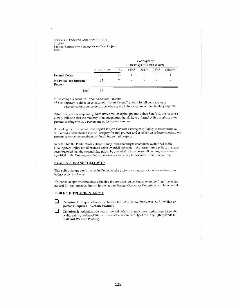
125
126

127
A.6 Naval Special Warfare Command: Control of MILCON Contingency Funds and Release AuthoritySan

128
129

130
A.7 Typical Contingency Drawdown from Managing Major Projects (MMP), (Source: htttps://managingmajorprojects.com)
Fig. A- 1 Typical Contingency Drawdown based on Activities
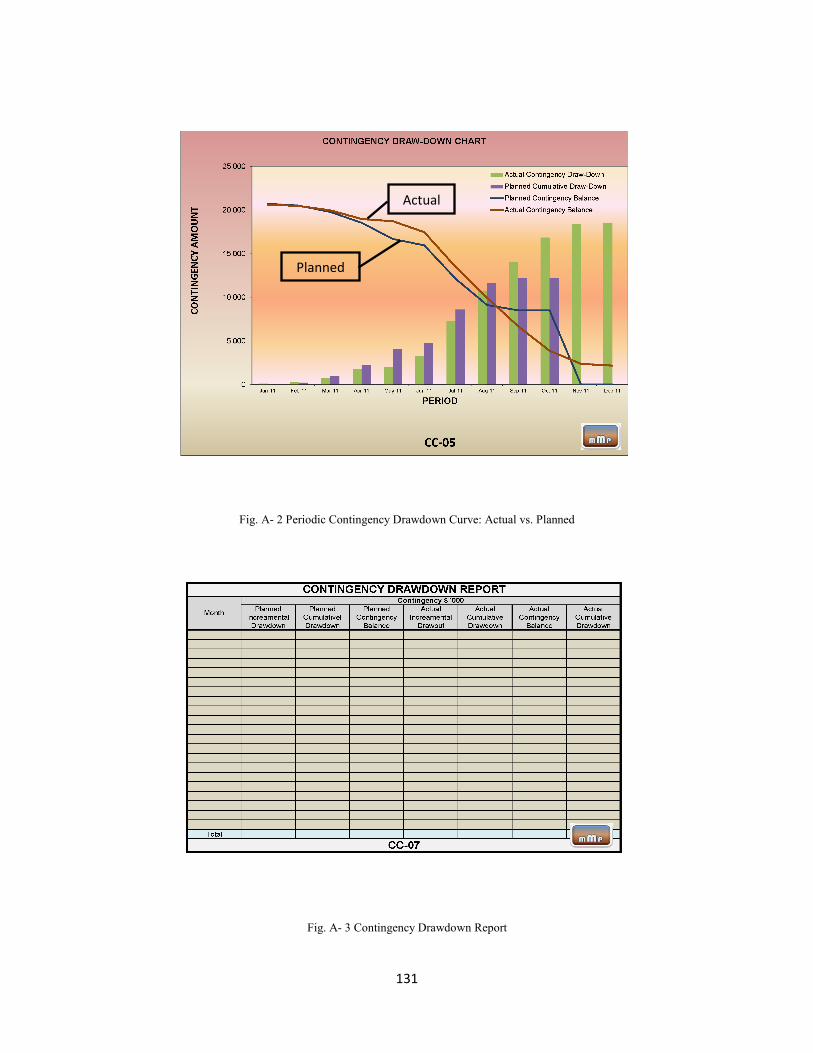
131
Fig. A- 2 Periodic Contingency Drawdown Curve: Actual vs. Planned
Fig. A- 3 Contingency Drawdown Report
Actual
Planned

132
A.8 NASA presentation: “Risk-Weighted Cost Estimates Principles and practical Application”
Fig. A- 4 Risk Weighted Cost Estimates Principles and Practical Application (NASA)
Fig. A- 5 Contingency Drawdown Curve and Project Milestones
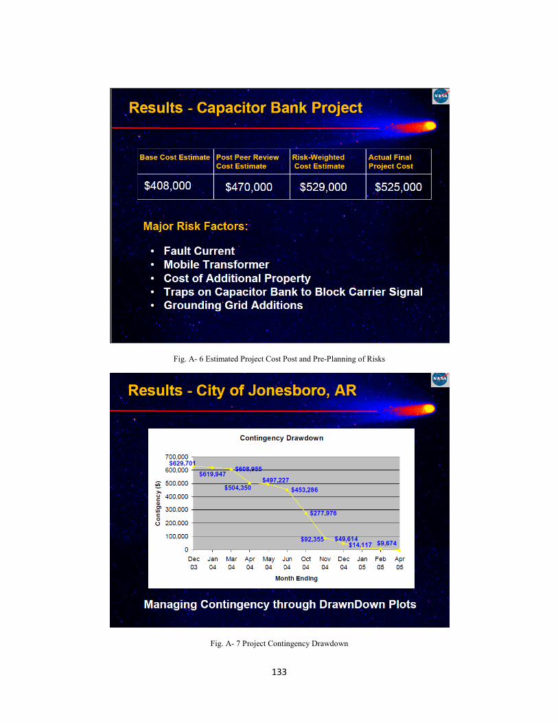
133
Fig. A- 6 Estimated Project Cost Post and Pre-Planning of Risks
Fig. A- 7 Project Contingency Drawdown
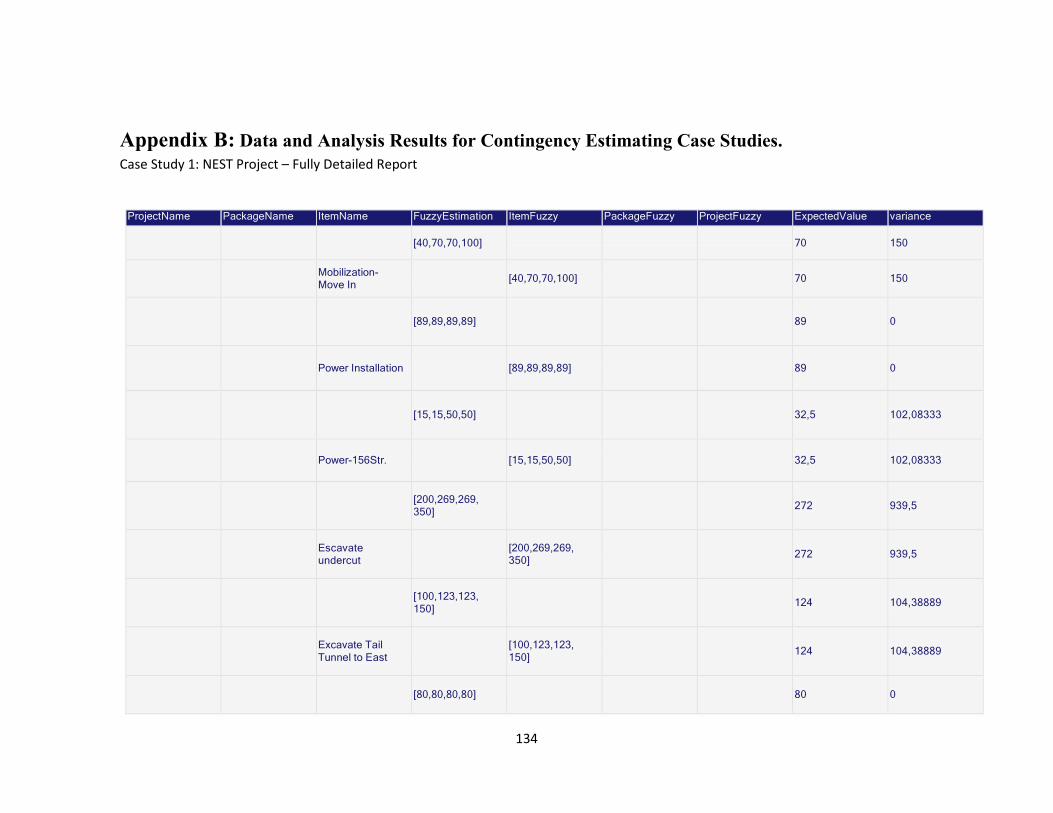
134
Appendix B: Data and Analysis Results for Contingency Estimating Case Studies. Case Study 1: NEST Project – Fully Detailed Report
ProjectName PackageName ItemName FuzzyEstimation ItemFuzzy PackageFuzzy ProjectFuzzy ExpectedValue variance
[40,70,70,100] 70 150
Mobilization- Move In [40,70,70,100] 70 150
[89,89,89,89] 89 0
Power Installation [89,89,89,89] 89 0
[15,15,50,50] 32,5 102,08333
Power-156Str. [15,15,50,50] 32,5 102,08333
[200,269,269, 350] 272 939,5
Escavate undercut [200,269,269,
350] 272 939,5
[100,123,123, 150] 124 104,38889
Excavate Tail Tunnel to East [100,123,123,
150] 124 104,38889
[80,80,80,80] 80 0

135
ProjectName PackageName ItemName FuzzyEstimation ItemFuzzy PackageFuzzy ProjectFuzzy ExpectedValue variance
Form and Pour Undercut [80 , 80 , 80 , 80] 80 0
[39,39,39,39] 39 0
Form and Pour TailUndercut [39,39,39,39] 39 0
[100,120,120, 150] 122,5 105,55556
Form and Pour Shaft [100,120,120,
150] 122,5 105,55556
[97,6,122,122, 146,4] 122 99,22667
Excavate Work Shaft [97,6,122,122,
146,4] 122 99,22667
Main Work Shaft [760,6,927, 962,1154,4] 951 9974,98879
[16,16,16,16] 16 0
Excavate Access Shaft [16,16,16,16] 16 0
[44,44,44,44] 44 0

136
ProjectName PackageName ItemName FuzzyEstimation ItemFuzzy PackageFuzzy ProjectFuzzy ExpectedValue variance
Backfill Shaft and Install [44 , 44 , 44 , 44] 44 0
Access Manhole [60,60,60,60] 60 0
[1952,2142,5, 2142,5,2910] 2286,75 42864,18056
Tunnel and Install Segments-866m [1952,2142,5,
2142,5,2910] 2286,75 42864,18056
[0,08,0,13, 0,13,0,14] 0,12 0,00017
Patch and Rub Tunnel Crown [0,08,0,13,
0,13,0,14] 0,12 0,00017
[0,16,0,19, 0,19,0,22] 0,19 0,00015
Patch and Rub Tunnel-Final Cleanup
[0,16,0,19, 0,19,0,22] 0,19 0,00015
[0,01,0,01, 0,01,0,01] 0,01 0
Spoil Removal [0,01,0,01, 0,01,0,01] 0,01 0
Tunneling(866m) [1952,25, 2142,83, 2142,83, 2910,37]
2287,07 42873,12007

137
ProjectName PackageName ItemName FuzzyEstimation ItemFuzzy PackageFuzzy ProjectFuzzy ExpectedValue variance
[61,61,61,61] 61 0
Access Manhole Shaft [61,61,61,61] 61 0
Access Manhole Shaft [61,61,61,61] 61 0
[1704,1870, 1870,2540] 1996 32648,66667
Tunnel and Install Segments(756 m)
[1704,1870, 1870,2540] 1996 32648,66667
[0,01,0,13, 0,13,0,14] 0,103 0,00087
Patch and Rub Tunnel Crown [0,01,0,13,
0,13,0,14] 0,103 0,00087
[0,16,0,19, 0,19,0,22] 0,19 0,00015
Patch and Rub Tunnel-Final Cleanup
[0,16,0,19, 0,19,0,22] 0,19 0,00015
[0,01,0,01, 0,01,0,01] 0,01 0
Spoil Removal [0,01,0,01, 0,01,0,01] 0,01 0
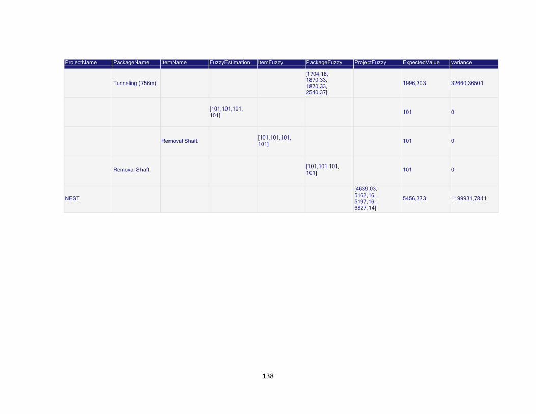
138
ProjectName PackageName ItemName FuzzyEstimation ItemFuzzy PackageFuzzy ProjectFuzzy ExpectedValue variance
Tunneling (756m) [1704,18, 1870,33, 1870,33, 2540,37]
1996,303 32660,36501
[101,101,101, 101] 101 0
Removal Shaft [101,101,101, 101] 101 0
Removal Shaft [101,101,101, 101] 101 0
NEST [4639,03, 5162,16, 5197,16, 6827,14]
5456,373 1199931,7811
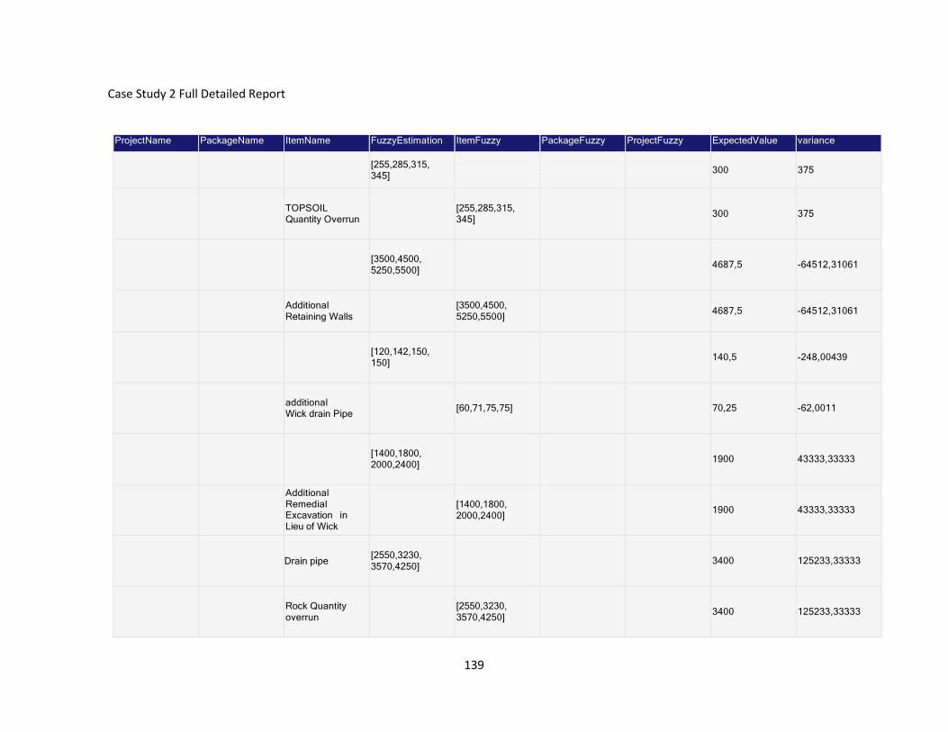
139
Case Study 2 Full Detailed Report
ProjectName PackageName ItemName FuzzyEstimation ItemFuzzy PackageFuzzy ProjectFuzzy ExpectedValue variance
[255,285,315, 345] 300 375
TOPSOIL Quantity Overrun [255,285,315,
345] 300 375
[3500,4500, 5250,5500] 4687,5 -64512,31061
Additional Retaining Walls [3500,4500,
5250,5500] 4687,5 -64512,31061
[120,142,150, 150] 140,5 -248,00439
additional Wick drain Pipe [60,71,75,75] 70,25 -62,0011
[1400,1800, 2000,2400] 1900 43333,33333
Additional Remedial Excavation in Lieu of Wick
[1400,1800, 2000,2400] 1900 43333,33333
Drain pipe [2550,3230, 3570,4250] 3400 125233,33333
Rock Quantity overrun [2550,3230,
3570,4250] 3400 125233,33333

140
ProjectName PackageName ItemName FuzzyEstimation ItemFuzzy PackageFuzzy ProjectFuzzy ExpectedValue variance
[2000,2375, 2625,3000] 2500 44270,83333
additional1mi hauling distance of drill and shoot rock
[2000,2375, 2625,3000] 2500 44270,83333
[4165,4753, 5047,5635] 4900 93639
disposalfee1$/ cu.yd. of drill and shoot rock [4165,4753,
5047,5635] 4900 93639
[1040,1170, 1430,1560] 1300 14083,33333
Increase in all Storm drainage pipeby6in
[1040,1170, 1430,1560] 1300 14083,33333
[1360,1615, 1700,1700] 1593,75 -34168,22917
Increase in reinforced concrete pipe
[1360,1615, 1700,1700] 1593,75 -34168,22917
[5250,6750, 7500,8625] 7031,25 221324,57386
schedule acceleration [5250,6750,
7500,8625] 7031,25 221324,57386
[800,900,1000, 1150] 962,5 10028,93519

141
ProjectName PackageName ItemName FuzzyEstimation ItemFuzzy PackageFuzzy ProjectFuzzy ExpectedValue variance
DBEby20% [800,900,1000 1150]
962,5 10028,93519
[3000,5100, 6600,7500] 5550 412500
Design Growth [3000,5100, 6600,7500] 5550 412500
[2800,3600, 4400,5200] 4000 266666,66667
design/approval delays [2800,3600,
4400,5200] 4000 266666,66667
[3750,4750, 5250,6000] 4937,5 91737,68939
Regulatory Agencies [3750,4750,
5250,6000] 4937,5 91737,68939
[4250,4750, 5000,5500] 4875 67708,33333
Disposal of Excess Materials [4250,4750,
5000,5500] 4875 67708,33333
UHCOC Positive Risk Elements [36180,45649,
51762,58440] 48007,75 9656609,11277
[-300,-300,- 297,-285] -295,5 -381,25

142
ProjectName PackageName ItemName FuzzyEstimation ItemFuzzy PackageFuzzy ProjectFuzzy ExpectedValue variance
Less remedial excavation [-300,-300,-
297,-285] -295,5 -381,25
[-4600,-4200,- 3800,-3200] -3950 16018,51852
Less retaining Wall sand pilings [-4600,-4200,-
3800,-3200] -3950 16018,51852
[-3000,-3000,- 2700,-2400] -2775 -25625
Fatten slopes on Site waste from drill and shoot rock
[-3000,-3000,- 2700,-2400] -2775 -25625
[-1256,-1133,- 1067,-935] -1097,75 3391,57703
less tire/track/repair cost
[-1256,-1133,- 1067,-935] -1097,75 3391,57703
[-1404,-1260,- 1140,-996] -1200 7536
Less equipment maintenance cost [-1404,-1260,-
1140,-996] -1200 7536
[-900,-900,- 873,-720] -848,25 -14119,60598
Piling reduction by 6ftperpileunder bridge
[-900,-900,- 873,-720] -848,25 -14119,60598

143
ProjectName PackageName ItemName FuzzyEstimation ItemFuzzy PackageFuzzy ProjectFuzzy ExpectedValue variance
[-2415,-2300,- 2185,-1725] -2156,25 -65692,03869
replace78R- value rock with 50R-value rock
[-2415,-2300,- 2185,-1725] -2156,25 -65692,03869
[-5750,-5000,- 4750,-3750] -4812,5 14612,26852
schedule deceleration [-5750,-5000,-
4750,-3750] -4812,5 14612,26852
[-2600,-2200,- 1800,-1400] -2000 66666,66667
Less design/ Approval delays [-2600,-2200,-
1800,-1400] -2000 66666,66667
UHCOC Negative Risk Elmenets [-22225,-20293,
-18612,-15411] -19135,25 -359516,59944
UHCOC [13955,25356, 33150,43029] 28872,5 33572723,87896