This is a repository copy of Fuzzy grey relational analysis for software effort estimation.

White Rose Research Online URL for this paper:http://eprints.whiterose.ac.uk/75052/

Version: Submitted Version

Article:

Azzeh, Mohammad, Neagu, Daniel and Cowling, Peter I. orcid.org/0000-0003-1310-6683 (2010) Fuzzy grey relational analysis for software effort estimation. Empirical Software Engineering. pp. 60-90. ISSN 1382-3256

https://doi.org/10.1007/s10664-009-9113-0

eprints@whiterose.ac.ukhttps://eprints.whiterose.ac.uk/

Reuse

Items deposited in White Rose Research Online are protected by copyright, with all rights reserved unless indicated otherwise. They may be downloaded and/or printed for private study, or other acts as permitted by national copyright laws. The publisher or other rights holders may allow further reproduction and re-use of the full text version. This is indicated by the licence information on the White Rose Research Online record for the item.

Takedown

If you consider content in White Rose Research Online to be in breach of UK law, please notify us by emailing eprints@whiterose.ac.uk including the URL of the record and the reason for the withdrawal request.

Fuzzy Grey Relational Analysis for Software Effort Estimation

MOHAMMAD AZZEH1, DANIEL NEAGU

2, PETER I. COWLING3

AI Research Centre, Department of Computing, University of Bradford,

Bradford, U.K., BD7 1DP 1M.Y.A.Azzeh@bradford.ac.uk, 2D.Neagu@bradford.ac.uk, 3P.I.Cowling@bradford.ac.uk

Abstract

Accurate and credible software effort estimation is a challenge for academic research and software industry. From

many software effort estimation models in existence, Estimation by Analogy (EA) is still one of the preferred

techniques by software engineering practitioners because it mimics the human problem solving approach. Accuracy

of such a model depends on the characteristics of the dataset, which is subject to considerable uncertainty. The

inherent uncertainty in software attribute measurement has significant impact on estimation accuracy because these

attributes are measured based on human judgment and are often vague and imprecise. To overcome this challenge

we propose a new formal EA model based on the integration of Fuzzy set theory with Grey Relational Analysis

(GRA). Fuzzy set theory is employed to reduce uncertainty in distance measure between two tuples at the kth

continuous feature ( |)k(x)k(x(| io ).GRA is a problem solving method that is used to assess the similarity

between two tuples with M features. Since some of these features are not necessary to be continuous and may have

nominal and ordinal scale type, aggregating different forms of similarity measures will increase uncertainty in the

similarity degree. Thus the GRA is mainly used to reduce uncertainty in the distance measure between two software

projects for both continuous and categorical features. Both techniques are suitable when relationship between effort

and other effort drivers is complex. Experimental results showed that using integration of GRA with FL produced

credible estimates when compared with the results obtained using Case-Based Reasoning, Multiple Linear

Regression and Artificial Neural Networks methods.

Keywords: Software Effort Estimation by Analogy, Similarity Measurement, Feature selection, Grey Relational

Analysis, Fuzzy Set Theory.

1. Introduction

Estimating the likely software project effort with high precision is still a largely unsolved problem. Although many software effort estimation models were developed in last three decades, none of them has consistently outperformed the others [28]. Amongst them, Estimation by Analogy (EA) [20] appears to be well suited to effort estimation, especially when the software product is poorly understood. EA is concerned with finding a solution for a new

problem based on known solutions from a set of similar problems. This requires a feature identification model [3] and a reliable similarity measurement [4]. EA is still a challenge for several reasons First, variability of data set structure including training dataset size, number of attributes, nominal and ordinal scale attributes, outliers, missing values, collinearity, etc. [32]. Second, software attribute identification and measurement is performed on the basis of human judgment which it is subject to considerable uncertainty [16, 23, 25]. In fact, software estimation involves identification and quantification of several predictive attributes that have significant impact on effort prediction. Thus, measuring these attributes should be performed in a consistent and robust way in order to avoid imprecision and vagueness. Third, the relationship between effort and other cost drivers is not often clear [21, 25].

Grey system theory provides a mathematical means to deal with uncertain and incomplete small data sets [33]. First developed by Deng [9, 10] to study the uncertainties in system models and help in prediction and decision making, Grey system theory is now applied in various fields such as decision making [13], system control [13], manufacturing [14] and transportation [14]. Grey Relational Analysis (GRA) is an important method of Grey System theory which used to determine the relationship (similarity) between two data tuples [14]. The tuple in our context represents to a project with M dimensional features. Given a reference tuple and a historical dataset, the GRA is used to assess the Grey Relation Grad (GRG) value between the reference tuple and each comparative tuple, then to determine the closest tuples to the reference tuple. The GRA can be viewed as a simple form of Case-Based Reasoning technique which utilizes the concept of absolute point-to-point distance between cases [33]. The attractiveness of GRA to software effort estimation stems from its flexibility to model complex nonlinear relationship between effort and cost drivers [13, 14]. Furthermore, The GRA has ability to learn from a small number of cases which is effective in the context of data-starvation [33]. Users may be more willing to accept a solution coming from the GRA since the idea of GRA is intuitively similar to human problem-solving behavior and hence may be easier for non-technical users to understand it [13].

The development of a software effort estimation model requires precision in attribute and similarity measurement, and the ability to learn from the structure of historical datasets. Fuzzy set theory [27] provides a representation scheme and mathematical operations for dealing with uncertain, imprecise and vague concepts. It also builds a formal quantitative model that captures the vagueness of human knowledge that is usually expressed in natural language. Thus, Fuzzy logic [36] is employed in the GRA learning processes to reduce uncertainty in similarity degree between reference tuple xo and comparative tuple xi at the kth continuous feature (denoted )k(oi =

|)k(x)k(x(| io ). For similarity measurement between categorical values we keep the same traditional fashion of

treatment which means zero when two categories at the kth categorical feature are equal and one when they are different. The similarity degree is later adjusted when the similarity between continuous and categorical data integrated and processed through GRA model. However, each data tuple as mentioned previously represents a software project with M feature dimensions. The integration of Fuzzy logic with GRA results in a new model called Fuzzy GRA (FGRA) which then is employed to develop a new software effort estimation model. The proposed model is considered as a form of EA and comprises four main stages: data preparation, feature identification, case retrievals and effort prediction. The FGRA is used to select the most predictive features based on the similarity between dependent feature and each independent feature. The features that present high similarity will set up the optimal feature set. The FGRA is also used to retrieve the closest projects to the reference project by measuring the similarity degree between reference project and all other comparative projects.

The proposed FGRA is validated against several well known software estimation models such as Case-Base Reasoning (CBR) [22], Artificial Neural Networks (ANN) [12] and Multiple Linear Regression (MLR) [13] based on five datasets: ISBSG [17], Desharnais [6], COCOMO‟81 [6], Kemerer [1] and Albrecht dataset (DP service) [19]. The results obtained from empirical evaluation are very encouraging in the sense of being comparable or better than other estimation models.

The present paper is organized as follows: section 2 presents a literature review about analogy software estimation. Section 3 introduces Fuzzy set theory. Section 4 introduces background about grey relational analysis. Section 5 describes the effort prediction using FGRA. Section 6 presents evaluation criteria MMRE, MdMRE, MMER and Pred(25). Section 7 presents the results obtained from empirical evaluation and comparisons to previous published results. Section 8 presents conclusion and directions for further work.

2. Related works

The GRA method is a relatively young in software effort estimation field. Little research has been carried out to exploit GRA in the software estimation process. Song et al. [33] proposed a software effort estimation method based on grey relational analysis called GRACE. They employed GRA to select an optimal feature set based on the similarity degree between dependent variable and other variables. The variables that exhibit large similarity are selected to form the optimal feature set. The variables are preferably continuous rather than categorical. The GRA is later used to derive new estimate by finding the closest case that approximately agrees with current case on all effort drivers. Their model outperformed other prediction models such as neural networks, decision tree and stepwise regression. On the other hand, Huang S.J. et al. [14] integrated GRA with genetic algorithms to improve software effort estimation. The genetic algorithm is used to adjust the weight factor associated with weighted GRA. Using genetic algorithm requires many parameters and assumptions to be setup before finding appropriate weights. However, experiments on various well established data sets revealed that the weighted GRA with genetic algorithms has significant impact on the accuracy of software effort estimation. Hsu et al. [13] proposed various weighted GRA models for software effort estimation. The investigated models are distance-based weight, linear weight, non-linear weight, maximal weight and correlative weight. They reported that weighted GRA performs better than non-weighted GRA in software effort estimation. The linearly weighted GRA outperforms other weighted GRA. Hsu et al. [13] investigated the applicability of GRA in analogy software effort estimation. In previous GRA-based estimation models, there is little attempt to deal with uncertainty in distance between two tuples at continuous and categorical features. Idri et al. [16] showed replacing categorical features (nominal or ordinal) by numerical values increases uncertainty in estimation. Therefore, in this work we use Fuzzy set theory and GRA to reduce imprecision in the distance between two projects containing continuous and categorical values.

In general, the accuracy of EA has been confirmed and evaluated in previous studies [2, 5, 20, 21, 22, 28, 29, 31, 32]. The remarkable observation from those studies that there is no consistent conclusion between them, some of them reported that EA is more effective than linear and stepwise regression [28, 29, 32]. Others [5, 31] come to different findings which contradict with Shepperd's findings. In [5, 31] it was shown that both EA and regression techniques improved estimation accuracy, but EA did not outperform regression. Idri et al. [16] proposed an alternative approach for EA model based on Fuzzy logic. They tried to adjust analogy estimation based on Fuzzy similarity between two software projects that are described only by ordinal data in the COCOMO dataset. This approach may not perform well over other datasets like ISBSG [17] that are structurally dissimilar to COCOMO dataset. Chiu et. al. [7] reported that EA always needs more sensed similarity methods. The effort obtained by these similarity methods is not always significant to be reused without processing. Thus, the similarity method needs adjustment to make the value of retrieved effort more reasonable. They investigated the use of genetic algorithm based project distance to adjust retrieved effort. The results showed that using adjusted similarity mechanism gave better accuracy than using traditional similarity distance.

Jorgensen et al. [18] used regression towards the mean method to adjust EA. The method is more suitable when the selected analogues are extreme and the estimation model inaccurate. They indicated that the adjusted estimation was significantly more accurate than EA without adjustment. Mittas et al [30] employed iterative resampling method to improve EA, they claimed that EA is closely related to formal nearest neighbor non parametric regression. On the other hand, Mendes et al.[28,29] investigated the use of CBR and adaptation rules on data collected from web hypermedia projects. The results revealed that using adaptation rules are not significant as did not contribute to better estimation.

3. Fuzzy set theory

Fuzzy set theory as introduced by Zadeh [37] provides a representation scheme and mathematical operations for dealing with uncertain, imprecise and vague concepts. Fuzzy model provides the formal framework to associate Fuzzy sets to linguistic values. Each Fuzzy set is described by membership function such as Triangle, Trapezoidal, Gaussian, etc., which assigns a membership value between 0 and 1 for each real point on universe of discourse. This membership value represents how much a particular point belongs to that Fuzzy set. For instance, consider the linguistic value low of feature Team_Experience, any element x of universe of discourse Team_Experience belongs to the Fuzzy set low as described by a membership function value low(x) [3]. In contrast, for crisp set

representations, the element x belongs to the set low if and only if x is one of the elements of the set low and is given by membership value one, otherwise zero. Fuzzy Logic provides a way to map between input and output space with clear natural expressions of Fuzzy rules [27]. A Fuzzy model can be constructed either by expert knowledge or using some learning algorithms. The former method uses expert experience that is then formulated as tuple of if-then-rules where parameters and memberships are tuned using input and output data [36]. The latter uses algorithms such as Fuzzy C-means (FCM) to create membership functions. The Fuzzy model proposed in this paper was constructed based on the second approach where membership functions are obtained by FCM [36].

The use of FCM algorithm to construct Fuzzy model requires prior determination of appropriate number of Fuzzy clusters (C). To do so, many clustering validity criteria have been proposed to measure the coherence of Fuzzy clustering. Amongst them, the Xie and Beni clustering validity criterion [35] as depicted in Eq. (1) has been used in this paper. A small value of XB means a more compact and separate clustering. The goal should therefore to minimize XB in order to have more coherence in Fuzzy clusters. We assume that the more compact Fuzzy clusters (i.e. coherent clusters) are the more useful to deliver a good prediction.

kiki

C

i

N

k kiij

CCN

xCuXB

,

1 1

2

min*

)( (1)

where iC is the ith center vector, u is the partition matrix, kx is the kth observation, and is Euclidian distance.

4. Grey relational analysis

GRA is an important method of Grey System theory [9, 10]. The word “grey” is used to represent the degree of information availability that is used to describe system structure. In particular terms, word "black" indicates that the required information used to describe system is entirely unavailable. Conversely, “white” indicates that the required internal information is entirely available. “Grey” stands for the information that is incomplete and rather unknown which comes between black and white [14]. GRA allows us to work on past experiences without need to have a complete dataset. GRA is one of the grey theory methods that use the grey relational coefficient (GRC) and the grey relations grade (GRG) to assess the overall similarity degree between two data tuples [13].

The concept behind GRA is grey space. Let X be a collection of n data tuples as shown in Eq. (2) where m represents number of features of each tuple.

)m(x...)(x)(x

............

)m(x...)(x)(x

)m(x...)(x)(x

X

nnn 21

21

21

222

111

(2)

The background of GRA is described through the following definitions:

Definition 1. Let P(X) be a factor set of grey relation which has the following properties [33]:

1. Availability of key attributes.

2. The number of attributes is known and limited.

3. Each attribute is measured independently.

4. The set of attributes is expandable which allows us to add new attributes later.

Definition 2. Let xo={ xo(1), xo(2),... xo(m)}P(X) be a reference tuple, and xi ={ xi(1), xi(2),..., xi(m)} P(X) be a comparator tuples; where xo(k), xi(k) representing respectively the numerals at column k for xo and xi. If

))k(x),k(x( io and )x,x( io are of real numbers, and satisfy the following four grey axioms, then

))k(x),k(x( io is called Grey Relation Coefficient and )x,x( io is called Grey Relation Grade which is the

average of ))k(x),k(x( io [33]. The relevant properties of Grey Relational Grade have been defined in [33].

Definition 3. Grey relational map (GRM): if )x,x( io satisfies the four grey relation axioms, then is called grey

relational map.

Definition 4. If satisfies the four grey relation axioms for P(X), then (P(X), ) is a grey relational space.

4.1 Grey relational coefficient

The Grey Relational Coefficient (GRC) [10, 14] is the process of finding, within the historical case base (comparative tuples), those tuples that are closest to the reference tuple. Suppose the reference tuple is xo={ xo(1), xo(2),... xo(m)}, and the comparative tuple is represented as xi ={ xi(1), xi(2),..., xi(m)} where i is in {1,2...n}. The formula of GRC at the kth attribute is given in Eq. (3). The distinguishing coefficient is used to minimize the

difference between )k(oi and )(max,

koiki .

1,0,)(max)(

)(max)(min))(),((

,

,,

kk

kkkxkx

oiki

oi

oiki

oiki

io (3)

where

)()(,1

)()(,0

,|)()(|

)(

kxkxandlcategoricaisfeaturekthewhen

kxkxandlcategoricaisfeaturekthewhen

numericisfeaturekthewhenkxkx

k

ioth

ioth

thio

oi

(4)

We made a significant modification to )(koi in order to incorporate the Fuzzy distance between two numeric

feature values. The goal of this new distance is to reduce uncertainty associated with similarity measurement at kth feature. As we mentioned above it is very hard to find distance between categorical data based on FCM unless we have sufficient information that differentiates between categories. Thus we intend to keep using the same style of treatment for categorical data at the kth feature (i.e. zero when categories at the kth categorical feature are equal and one when they are different). The aggregated distances between continuous data and categorical data are then

processed together using GRA to reduce uncertainty in all features. The proposed new distance )k(oi is an

extension of our proposed work in [4] which aims to assess the similarity measurement between two software projects based on FCM. In previous work [4] we showed that the use of Fuzzy modeling based on FCM improved the prediction accuracy because: (1) it reduces the uncertainty in similarity measurement. The main problem in conventional EA is that we are more likely to find two projects are similar in terms of their features but their effort value are completely different therefore the proposed method mitigated this problem by handling uncertainty in the similarity measurement. (2) Using FCM algorithm has also the advantage to group closest projects together in the same Fuzzy cluster and therefore boosts project retrieval. On the other hand, the approach proposed in [4] still has several limitations: first, the similarity degree between two different feature values fall in the same Fuzzy set is equal to 1 as similarity degree between a project to itself. Second, the approach was restricted to Gaussian membership function. The proposed Fuzzy distance in this paper attempts to overcome these challenges by proposing more general formula based on the concept of Fuzzy set theory that can be applied to different membership functions. Furthermore, we add the adjustment ratiok to make sure that the distance between two

different projects fall in the same Fuzzy sets does not equal to 0. The modified )(koi is shown in Eq. (5).

)()(,1

)()(,0

,)(,)(min*1

)(

kxkxandlcategoricaisfeaturekthewhen

kxkxandlcategoricaisfeaturekthewhen

numericisfeaturekthewhenPPPP

k

ioth

ioth

thkiokiok

oi

(5)

)])(),([minmax()( ttPPio

kPP

Ttkio

(6)

)])(),([maxmin()( ttPPio

kPP

Ttkio

(7)

))x(),x(max(

))x(),x(min(

iPoP

iPoPk

io

io

(8)

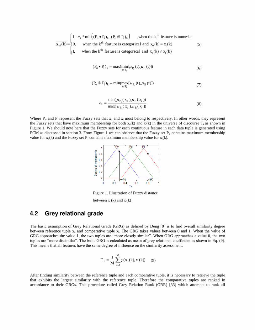
Where Po and Pi represent the Fuzzy sets that xo and xi most belong to respectively. In other words, they represent the Fuzzy sets that have maximum membership for both xo(k) and xi(k) in the universe of discourse Tk as shown in Figure 1. We should note here that the Fuzzy sets for each continuous feature in each data tuple is generated using FCM as discussed in section 3. From Figure 1 we can observe that the Fuzzy set Po contains maximum membership value for xo(k) and the Fuzzy set Pi contains maximum membership value for xi(k).

Figure 1. Illustration of Fuzzy distance

between xo(k) and xi(k)

4.2 Grey relational grade

The basic assumption of Grey Relational Grade (GRG) as defined by Deng [9] is to find overall similarity degree between reference tuple xo and comparative tuple xi. The GRG takes values between 0 and 1. When the value of GRG approaches the value 1, the two tuples are “more closely similar”. When GRG approaches a value 0, the two tuples are “more dissimilar”. The basic GRG is calculated as mean of grey relational coefficient as shown in Eq. (9). This means that all features have the same degree of influence on the similarity assessment.

M

kiooi kxkx

M1

))(),((1 (9)

After finding similarity between the reference tuple and each comparative tuple, it is necessary to retrieve the tuple that exhibits the largest similarity with the reference tuple. Therefore the comparative tuples are ranked in accordance to their GRGs. This procedure called Grey Relation Rank (GRR) [33] which attempts to rank all

FGRA Software Effort Estimation ^E

Estimated effort

comparative tuples according to their similarity with reference tuple. If )x,x(...)x,x()x,x( qojoio then

qji x...xx is the grey relation order.

5. FGRA software effort estimation model

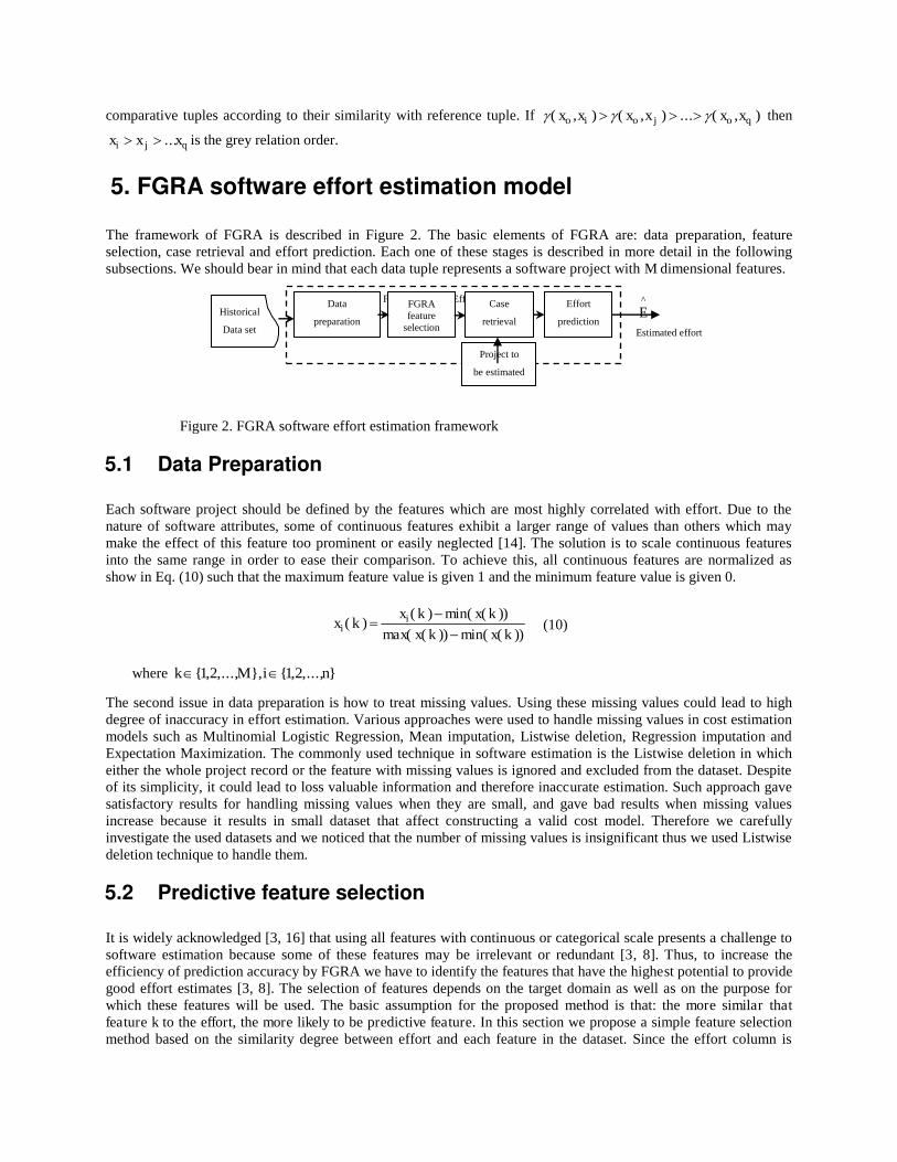
The framework of FGRA is described in Figure 2. The basic elements of FGRA are: data preparation, feature selection, case retrieval and effort prediction. Each one of these stages is described in more detail in the following subsections. We should bear in mind that each data tuple represents a software project with M dimensional features.

Figure 2. FGRA software effort estimation framework

5.1 Data Preparation

Each software project should be defined by the features which are most highly correlated with effort. Due to the nature of software attributes, some of continuous features exhibit a larger range of values than others which may make the effect of this feature too prominent or easily neglected [14]. The solution is to scale continuous features into the same range in order to ease their comparison. To achieve this, all continuous features are normalized as show in Eq. (10) such that the maximum feature value is given 1 and the minimum feature value is given 0.

))k(xmin())k(xmax(

))k(xmin()k(x)k(x i

i

(10)

where },...,2,1{},,...,2,1{ niMk

The second issue in data preparation is how to treat missing values. Using these missing values could lead to high degree of inaccuracy in effort estimation. Various approaches were used to handle missing values in cost estimation models such as Multinomial Logistic Regression, Mean imputation, Listwise deletion, Regression imputation and Expectation Maximization. The commonly used technique in software estimation is the Listwise deletion in which either the whole project record or the feature with missing values is ignored and excluded from the dataset. Despite of its simplicity, it could lead to loss valuable information and therefore inaccurate estimation. Such approach gave satisfactory results for handling missing values when they are small, and gave bad results when missing values increase because it results in small dataset that affect constructing a valid cost model. Therefore we carefully investigate the used datasets and we noticed that the number of missing values is insignificant thus we used Listwise deletion technique to handle them.

5.2 Predictive feature selection

It is widely acknowledged [3, 16] that using all features with continuous or categorical scale presents a challenge to software estimation because some of these features may be irrelevant or redundant [3, 8]. Thus, to increase the efficiency of prediction accuracy by FGRA we have to identify the features that have the highest potential to provide good effort estimates [3, 8]. The selection of features depends on the target domain as well as on the purpose for which these features will be used. The basic assumption for the proposed method is that: the more similar that feature k to the effort, the more likely to be predictive feature. In this section we propose a simple feature selection method based on the similarity degree between effort and each feature in the dataset. Since the effort column is

Historical

Data set

Data

preparation

FGRA feature

selection

Case

retrieval

Effort

prediction

Project to

be estimated

regarded as numeric feature therefore it is not reasonable to assess its similarity degree with categorical attribute. Thus, the proposed feature selection method is divided into two stages, the first stage attempts to identify the best continuous features set among all continuous features. The second stage start adding one categorical feature at a time to the best continuous features set from stage one, and assessing its fitness on the prediction accuracy. The proposed feature selection method is described in the following steps:

Stage 1: For numerical features

Step 1.1: Let xo={ e1, e2,... en} be effort tuple, xi = {x1(i), x2(i),..., xn(i)}, }m,...,,{i 21 be the ith feature

tuple.

Step 1.2: Calculate GRG between reference feature tuple and each comparative feature tuple using the following modified GRG equation as depicted in Eq. (11). This modification allows us to narrowing the interval between min and max to be within [0, 1].

oii

oi

oii

oii

io xx

max

maxmin),( (11)

M

koioi k

Mwhere

1

)(1

(12)

where M represents a number of columns in data set and i is a row number.

Step 1.3: Choose only xi, }m,...,,{i 21 where the GRG is above the mean of all GRGs, as the optimal

feature set.

Stage 2: For categorical features.

After determining the optimal continuous feature set, the next step is to assess the impact of incorporating categorical features on the prediction accuracy.

Step 2.1: If there are categorical features in the dataset, then start adding one feature a time to the current continuous feature set and assess the fitness of selected features on the prediction accuracy.

Step 2.2: If the added categorical feature did not improve prediction accuracy, it is excluded from the current feature set; otherwise the categorical feature is kept. Then go to step 2.1.

Function FeatureSelection For i =1, i <= M, i++ Do

If (xi is numeric) then:

GRG(i)=Find ),( io xx ;

End_IF; End_For; Optimal _Feature_Set=best_Features(GRGs); Current_Fitness=Fitness(Optimal _Feature_Set) For j =1, j <=M, j++ Do

If (xj is categorical) then: Add xj to Optimal _Feature_Set; If Fitness(Optimal _Feature_Set) is poor then: Remove xj from Optimal _Feature_Set;

End_IF; End_IF;

End_For

Return Optimal _Feature_Set

5.3 Case retrieval

Case retrieval stage in FGRA aims to retrieve the historical projects that exhibit large similarity with project under

investigation. Using the proposed distance )k(oi between two tuples at kth feature, the new GRC formula is shown

in Eq. (13). Hence, the continuous data should be initially fuzzified using FCM [3, 4, 48] before calculating the distance.

)(max)(

)(max)(min))(),((

,

,,

kk

kkkxkx

oiki

oi

oiki

oiki

io

(13)

After finding all GRCs between the reference project and ith comparative project, the )x,x( io values are calculated

for each i according to Eq. (9). The range of )x,x( io is from 0 to 1 in each case. Zero means that two projects are

completely dissimilar, while one means that two projects are identical.

5.4 Effort prediction

The effort prediction stage derives final effort estimate based on the retrieved projects. In this stage we have to determine the number of retrieved projects that should be involved in the effort prediction. In the literature [5, 16, 28, 29], there are two perspectives, the first one attempts to involve all projects that fall within a particular distance of new project [16]. This approach could ignore some projects which might contribute data when distance between selected and unselected projects is negligible. For example, assume that the similarity between reference project and retrieved four projects (p1, p2, p3, p4) are 0.9, 0.86, 0.8 and 0.79 respectively and the strategy used in effort prediction is to employ only the comparative projects that have similarity degree over or equal to 0.8. In this case p4

is not considered even though the difference between p4 and p3 is small and it may be that p4 is a better predictor than p3. The second approach from literature is to use a fixed number of retrieved projects. This approach has been followed by many researchers such as [5, 28, 29]. The second approach has been followed in this research where number of analogies is 3 as suggested by Mendes et al. [29] and Sheppered et al. [32], which we believe is sufficient to derive a good estimate [28].

Before deriving final estimate, all GRGs must be ranked in order to have the closest projects to current one. After that, we adjust each retrieved project according to its GRCs with the reference project as shown in Eq. (14), then the final effort estimate is derived based on normalized GRGs as shown in Eq. (15). Ranking all GRGs in order provide us the order of closest projects to reference project.

M

jM

jio

iiooi

))j(x),j(x(

E*))j(x),j(x(E

1

1

(14)

3

1ioiio

^E*)x,x(E (15)

where: iE is the ith closest analogy.

oiE is the ith adapted analogy.

^E is the final prediction.

is the normalized GRG of closest analogies.

6. Evaluation criteria

For the purpose of evaluation and validation, it is necessary to measure how accurate the software estimates are. In this context, we used the common evaluation criteria in the field of software engineering [28]:

(i) Magnitude Relative Error (MRE) computes the absolute percentage of error between actual and predicted effort for each reference project.

i

iii actual

|estimatedactual|MRE

- (16)

(ii ) Mean Magnitude Relative Error (MMRE) calculates the average of MREs over all reference projects. Since the MMRE is sensitive to an individual outlying prediction, when we have a large number of observations, we adopt median of MREs for the n projects (MdMRE) which is less sensitive to the extreme values of MRE. Despite of the widely used of MMRE in estimation accuracy, there has been a substantive discussion about efficacy of MMRE in estimation process. MMRE has been criticised that is unbalanced in many validation circumstances and leads often to overestimation [32]. Therefore we used alternative accuracy indicator called magnitude of relative error relative to the estimate (MMER) to alleviate the problem of overestimation and underestimation.

䌥1

1n

i

iMREn

MMRE

(17)

)( ii

MREmedianMdMRE (18)

n

i i

ii

estimated

estimatedactual

nMMER

1

1

(19)

(iii ) Pred ( ) is used as complementary criterion to count the percentage of estimates that fall within less than of the actual values. The common used value for is 25% and that a good prediction system should offer this accuracy level 75% of the time.

100* =)Pred(n

(20)

Where is the number of projects where %iMRE , and n is the number of all observations. A software

estimation model with lower MMRE, MdMRE, and higher Pred(25) shows its derived estimates are more accurate than other models. We also used Boxplot of absolute residuals as alternatives to simple summary measures because they can give a good indication of the distribution of residuals and can help explain summary statistics such as MMRE and Pred(25). On the other hand, MMRE is not always reliable to compare between prediction methods because it is quite related to the measure of MRE spread therefore we used one-sample Wilcoxon signed rank test and Mann-Whitney U test to investigate the statistical significance of all the results, setting the confidence limit at 0.05. The Wilcoxon signed rank test is a nonparametric test that compares the median of a sample of numbers against a

hypothetical median. The reason behind using these tests is because all absolute residuals for all the models used in this study were not normally distributed.

7 Results and Discussions

7.1 Datasets

For the purpose of model evaluation we have used five well established datasets which they exhibit typical characteristics of software effort estimation dataset. Thus, we believe that using all of these datasets is sufficient to validate our models. These datasets come from different sources: ISBSG (release 10, 2007) [17], Desharnais [6], Kemerer [19], Albrecht [1] (IBM DP service) and COCOMO‟81 [6]. The descriptive statistics of the datasets are given in Table 1. The datasets present a range of effort values (expressed using different units). Each dataset is treated separately because each one has different features and so the datasets cannot be merged in one large dataset.

Table 1. Descriptive statistics of the datasets

Dataset Cases Categorical Features

Numerical Features

Effort mean

Effort Std.

ISBSG 107 1 8 14668 11727 (hours) Desharnais 77 1 10 4834 4188 (hours) COCOMO‟81 63 2 15 406.4 657 (man-month) Kemerer 15 2 4 219.25 263(man-month) IBM DP Service 24 1 6 21875 28417(hours)

7.1.1 ISBSG dataset

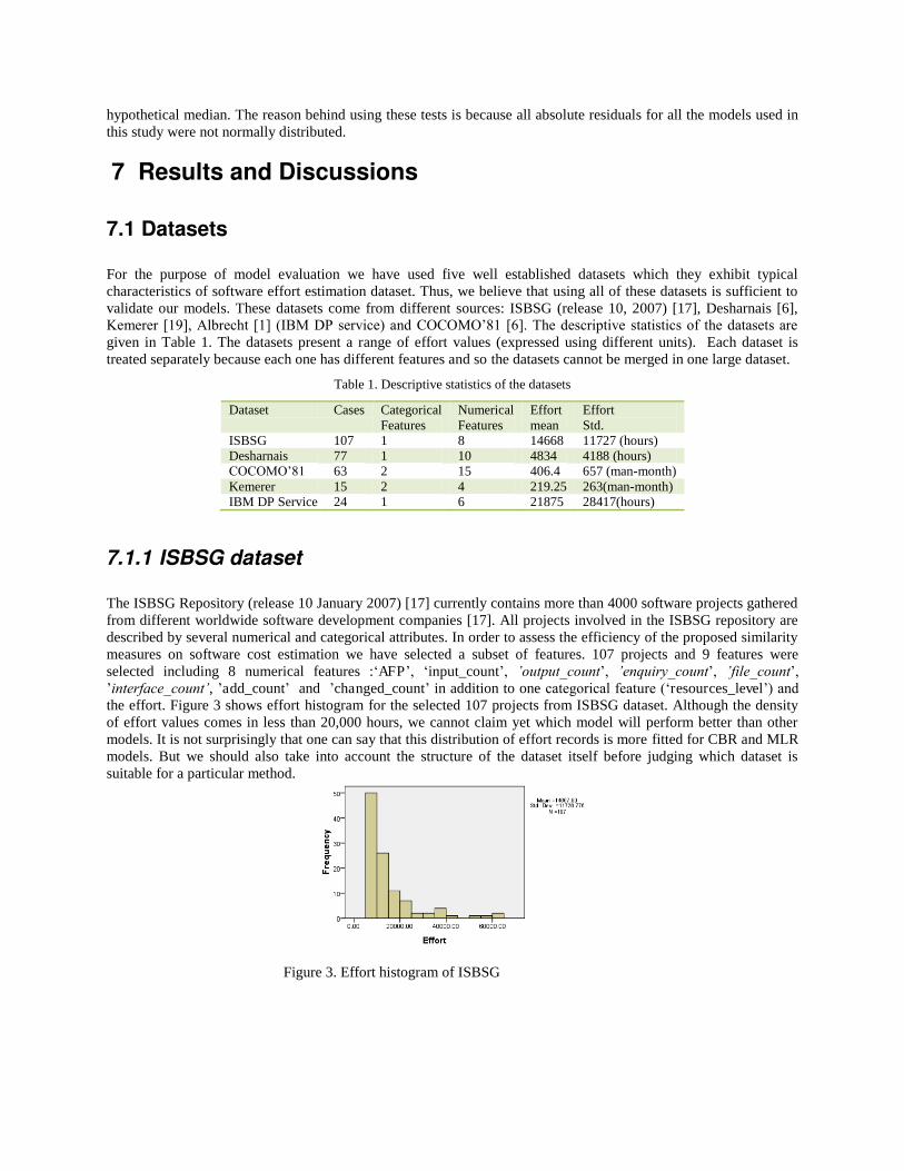
The ISBSG Repository (release 10 January 2007) [17] currently contains more than 4000 software projects gathered from different worldwide software development companies [17]. All projects involved in the ISBSG repository are described by several numerical and categorical attributes. In order to assess the efficiency of the proposed similarity measures on software cost estimation we have selected a subset of features. 107 projects and 9 features were selected including 8 numerical features :„AFP‟, „input_count‟, ’output_count‟, ’enquiry_count‟, ’file_count‟, ‟interface_count’, ‟add_count‟ and ‟changed_count‟ in addition to one categorical feature („resources_level‟) and the effort. Figure 3 shows effort histogram for the selected 107 projects from ISBSG dataset. Although the density of effort values comes in less than 20,000 hours, we cannot claim yet which model will perform better than other models. It is not surprisingly that one can say that this distribution of effort records is more fitted for CBR and MLR models. But we should also take into account the structure of the dataset itself before judging which dataset is suitable for a particular method.

Figure 3. Effort histogram of ISBSG

7.1.2 Desharnais dataset

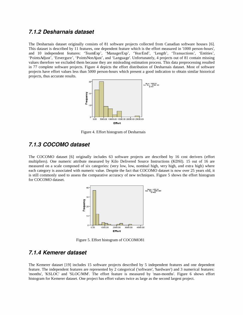
The Desharnais dataset originally consists of 81 software projects collected from Canadian software houses [6]. This dataset is described by 11 features, one dependent feature which is the effort measured in '1000 person-hours', and 10 independent features: „TeamExp‟, „ManagerExp‟, „YearEnd‟, „Length‟, „Transactions‟, „Entities‟, „PointsAdjust‟, „Envergure‟, „PointsNonAjust‟, and „Language'. Unfortunately, 4 projects out of 81 contain missing values therefore we excluded them because they are misleading estimation process. This data preprocessing resulted in 77 complete software projects. Figure 4 depicts the effort distribution of Desharnais dataset. Most of software projects have effort values less than 5000 person-hours which present a good indication to obtain similar historical projects, thus accurate results.

Figure 4. Effort histogram of Desharnais

7.1.3 COCOMO dataset

The COCOMO dataset [6] originally includes 63 software projects are described by 16 cost derivers (effort multipliers). One numeric attribute measured by Kilo Delivered Source Instructions (KDSI). 15 out of 16 are measured on a scale composed of six categories: (very low, low, nominal high, very high, and extra high) where each category is associated with numeric value. Despite the fact that COCOMO dataset is now over 25 years old, it is still commonly used to assess the comparative accuracy of new techniques. Figure 5 shows the effort histogram for COCOMO dataset.

Figure 5. Effort histogram of COCOMO81

7.1.4 Kemerer dataset

The Kemerer dataset [19] includes 15 software projects described by 5 independent features and one dependent feature. The independent features are represented by 2 categorical ('software', 'hardware') and 3 numerical features: 'months', 'KSLOC' and 'SLOC/MM'. The effort feature is measured by 'man-months'. Figure 6 shows effort histogram for Kemerer dataset. One project has effort values twice as large as the second largest project.

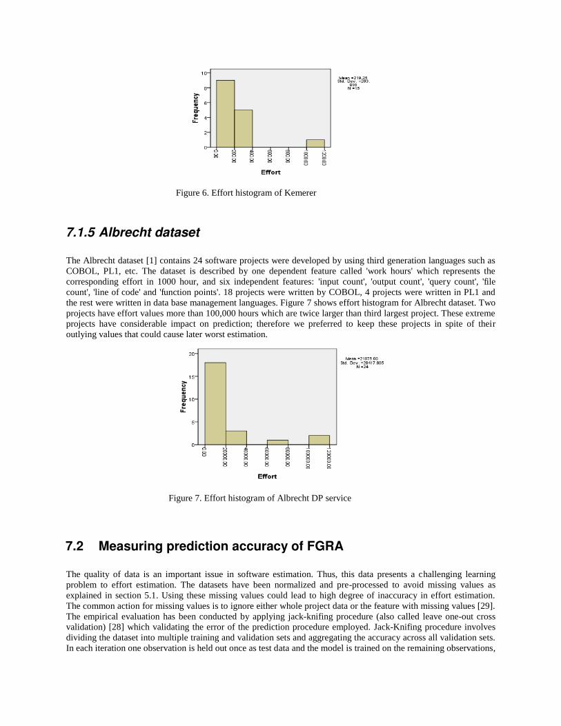
Figure 6. Effort histogram of Kemerer

7.1.5 Albrecht dataset

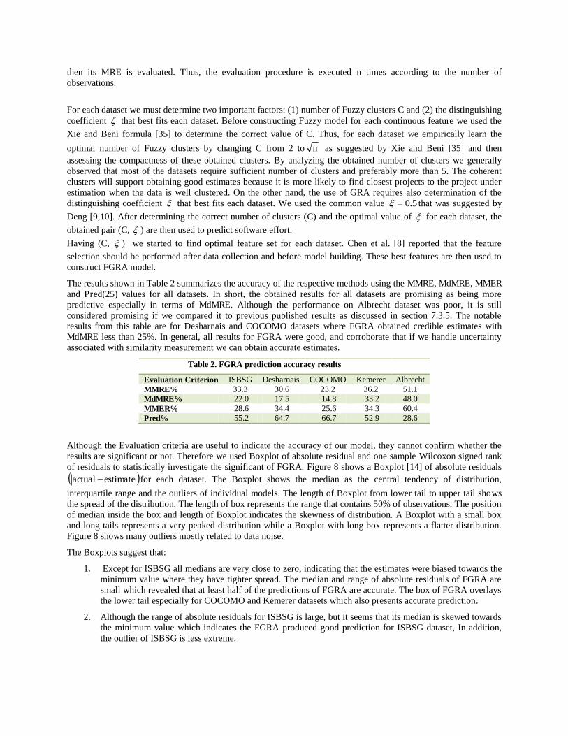
The Albrecht dataset [1] contains 24 software projects were developed by using third generation languages such as COBOL, PL1, etc. The dataset is described by one dependent feature called 'work hours' which represents the corresponding effort in 1000 hour, and six independent features: 'input count', 'output count', 'query count', 'file count', 'line of code' and 'function points'. 18 projects were written by COBOL, 4 projects were written in PL1 and the rest were written in data base management languages. Figure 7 shows effort histogram for Albrecht dataset. Two projects have effort values more than 100,000 hours which are twice larger than third largest project. These extreme projects have considerable impact on prediction; therefore we preferred to keep these projects in spite of their outlying values that could cause later worst estimation.

Figure 7. Effort histogram of Albrecht DP service

7.2 Measuring prediction accuracy of FGRA

The quality of data is an important issue in software estimation. Thus, this data presents a challenging learning problem to effort estimation. The datasets have been normalized and pre-processed to avoid missing values as explained in section 5.1. Using these missing values could lead to high degree of inaccuracy in effort estimation. The common action for missing values is to ignore either whole project data or the feature with missing values [29]. The empirical evaluation has been conducted by applying jack-knifing procedure (also called leave one-out cross validation) [28] which validating the error of the prediction procedure employed. Jack-Knifing procedure involves dividing the dataset into multiple training and validation sets and aggregating the accuracy across all validation sets. In each iteration one observation is held out once as test data and the model is trained on the remaining observations,

then its MRE is evaluated. Thus, the evaluation procedure is executed n times according to the number of observations.

For each dataset we must determine two important factors: (1) number of Fuzzy clusters C and (2) the distinguishing coefficient that best fits each dataset. Before constructing Fuzzy model for each continuous feature we used the

Xie and Beni formula [35] to determine the correct value of C. Thus, for each dataset we empirically learn the

optimal number of Fuzzy clusters by changing C from 2 ton as suggested by Xie and Beni [35] and then assessing the compactness of these obtained clusters. By analyzing the obtained number of clusters we generally observed that most of the datasets require sufficient number of clusters and preferably more than 5. The coherent clusters will support obtaining good estimates because it is more likely to find closest projects to the project under estimation when the data is well clustered. On the other hand, the use of GRA requires also determination of the distinguishing coefficient that best fits each dataset. We used the common value 5.0 that was suggested by

Deng [9,10]. After determining the correct number of clusters (C) and the optimal value of for each dataset, the

obtained pair (C, ) are then used to predict software effort.

Having (C, ) we started to find optimal feature set for each dataset. Chen et al. [8] reported that the feature

selection should be performed after data collection and before model building. These best features are then used to construct FGRA model.

The results shown in Table 2 summarizes the accuracy of the respective methods using the MMRE, MdMRE, MMER and Pred(25) values for all datasets. In short, the obtained results for all datasets are promising as being more predictive especially in terms of MdMRE. Although the performance on Albrecht dataset was poor, it is still considered promising if we compared it to previous published results as discussed in section 7.3.5. The notable results from this table are for Desharnais and COCOMO datasets where FGRA obtained credible estimates with MdMRE less than 25%. In general, all results for FGRA were good, and corroborate that if we handle uncertainty associated with similarity measurement we can obtain accurate estimates.

Table 2. FGRA prediction accuracy results

Evaluation Criterion ISBSG Desharnais COCOMO Kemerer Albrecht MMRE% 33.3 30.6 23.2 36.2 51.1 MdMRE% 22.0 17.5 14.8 33.2 48.0 MMER% 28.6 34.4 25.6 34.3 60.4 Pred% 55.2 64.7 66.7 52.9 28.6

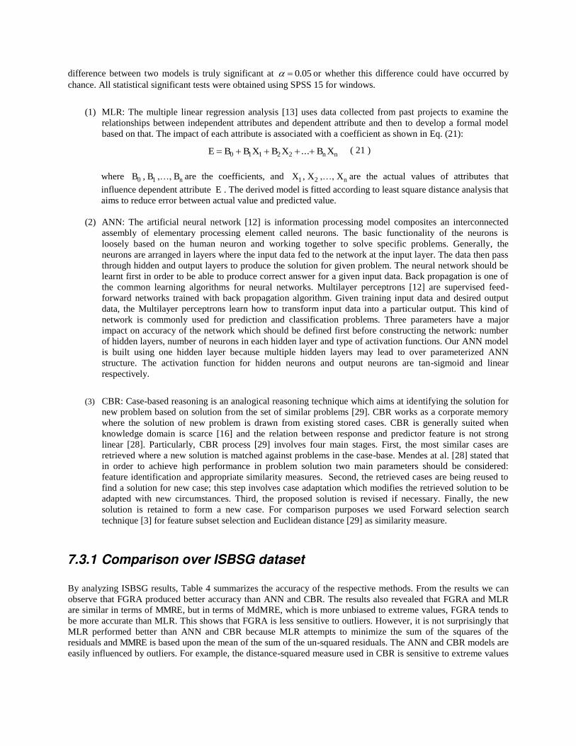
Although the Evaluation criteria are useful to indicate the accuracy of our model, they cannot confirm whether the results are significant or not. Therefore we used Boxplot of absolute residual and one sample Wilcoxon signed rank of residuals to statistically investigate the significant of FGRA. Figure 8 shows a Boxplot [14] of absolute residuals estimateactual for each dataset. The Boxplot shows the median as the central tendency of distribution,

interquartile range and the outliers of individual models. The length of Boxplot from lower tail to upper tail shows the spread of the distribution. The length of box represents the range that contains 50% of observations. The position of median inside the box and length of Boxplot indicates the skewness of distribution. A Boxplot with a small box and long tails represents a very peaked distribution while a Boxplot with long box represents a flatter distribution. Figure 8 shows many outliers mostly related to data noise.

The Boxplots suggest that:

1. Except for ISBSG all medians are very close to zero, indicating that the estimates were biased towards the minimum value where they have tighter spread. The median and range of absolute residuals of FGRA are small which revealed that at least half of the predictions of FGRA are accurate. The box of FGRA overlays the lower tail especially for COCOMO and Kemerer datasets which also presents accurate prediction.

2. Although the range of absolute residuals for ISBSG is large, but it seems that its median is skewed towards the minimum value which indicates the FGRA produced good prediction for ISBSG dataset, In addition, the outlier of ISBSG is less extreme.

To investigate the statistical significance of FGRA on each dataset we used one-sample Wilcoxon signed rank test for residuals as shown in Table 3, setting test value to zero. In this test if the resulting p-value is small (p<0.05), then the sample data are not symmetrical about the test value and therefore a statistically significant difference can be accepted between the sample median and the test value. The residuals obtained using the FGRA model were not significantly different from the test value zero. This suggests that the data do not give any reason to conclude that the residuals median differs from the hypothetical median (test value). So we can safely conclude that the medians of residuals generated by FGRA are not different from zero but it is not exactly same. Thus, there is advantage to these datasets obtaining their effort estimations using our proposed FGRA model.

Table 3. FGRA Statistical results based on residuals

Statistical measure ISBSG Desharnais COCOMO Kemerer Albrecht P-value 0.421 0.077 0.354 0.5506 0.2136 Sum of signed ranks (W) -414 698 193 22 28

Figure 8 Boxplot of absolute residuals

7.3 Comparison of FGRA to Case-based reasoning, Adaptive neural

networks and Multiple linear regression

This section presents the results obtained when we compared FGRA model to artificial neural networks (ANN) [12], multiple linear regression (MLR) [13] and case-based reasoning (CBR) [22]. We should note here that both ANN and MLR are applied only to numerical features. To determine their prediction accuracy we used leave one out cross validation approach as explained in section 7.2. For the comparison purpose, we apply Wrapper feature selection method based on forward searching strategy [8, 22] to CBR, ANN, and MLR techniques in order to obtain the most predictive features for each technique. However, in this section we addressed the impact of feature selection on the compared models and investigate whether they produce better results than FGRA or not. We also used Boxplot of absolute residuals to statistically measure the distribution of residuals. Based on absolute residuals we test the statistical significant of all the results. To do so we used the Mann-Whitney U test in order to tell us whether the

difference between two models is truly significant at 05.0 or whether this difference could have occurred by chance. All statistical significant tests were obtained using SPSS 15 for windows.

(1) MLR: The multiple linear regression analysis [13] uses data collected from past projects to examine the

relationships between independent attributes and dependent attribute and then to develop a formal model based on that. The impact of each attribute is associated with a coefficient as shown in Eq. (21):

nnXBXBXBBE ...22110 ( 21 )

where 0B , 1B ,…, nB are the coefficients, and 1X , 2X ,…, nX are the actual values of attributes that

influence dependent attribute E . The derived model is fitted according to least square distance analysis that aims to reduce error between actual value and predicted value.

(2) ANN: The artificial neural network [12] is information processing model composites an interconnected

assembly of elementary processing element called neurons. The basic functionality of the neurons is loosely based on the human neuron and working together to solve specific problems. Generally, the neurons are arranged in layers where the input data fed to the network at the input layer. The data then pass through hidden and output layers to produce the solution for given problem. The neural network should be learnt first in order to be able to produce correct answer for a given input data. Back propagation is one of the common learning algorithms for neural networks. Multilayer perceptrons [12] are supervised feed-forward networks trained with back propagation algorithm. Given training input data and desired output data, the Multilayer perceptrons learn how to transform input data into a particular output. This kind of network is commonly used for prediction and classification problems. Three parameters have a major impact on accuracy of the network which should be defined first before constructing the network: number of hidden layers, number of neurons in each hidden layer and type of activation functions. Our ANN model is built using one hidden layer because multiple hidden layers may lead to over parameterized ANN structure. The activation function for hidden neurons and output neurons are tan-sigmoid and linear respectively.

(3) CBR: Case-based reasoning is an analogical reasoning technique which aims at identifying the solution for new problem based on solution from the set of similar problems [29]. CBR works as a corporate memory where the solution of new problem is drawn from existing stored cases. CBR is generally suited when knowledge domain is scarce [16] and the relation between response and predictor feature is not strong linear [28]. Particularly, CBR process [29] involves four main stages. First, the most similar cases are retrieved where a new solution is matched against problems in the case-base. Mendes at al. [28] stated that in order to achieve high performance in problem solution two main parameters should be considered: feature identification and appropriate similarity measures. Second, the retrieved cases are being reused to find a solution for new case; this step involves case adaptation which modifies the retrieved solution to be adapted with new circumstances. Third, the proposed solution is revised if necessary. Finally, the new solution is retained to form a new case. For comparison purposes we used Forward selection search technique [3] for feature subset selection and Euclidean distance [29] as similarity measure.

7.3.1 Comparison over ISBSG dataset

By analyzing ISBSG results, Table 4 summarizes the accuracy of the respective methods. From the results we can observe that FGRA produced better accuracy than ANN and CBR. The results also revealed that FGRA and MLR are similar in terms of MMRE, but in terms of MdMRE, which is more unbiased to extreme values, FGRA tends to be more accurate than MLR. This shows that FGRA is less sensitive to outliers. However, it is not surprisingly that MLR performed better than ANN and CBR because MLR attempts to minimize the sum of the squares of the residuals and MMRE is based upon the mean of the sum of the un-squared residuals. The ANN and CBR models are easily influenced by outliers. For example, the distance-squared measure used in CBR is sensitive to extreme values

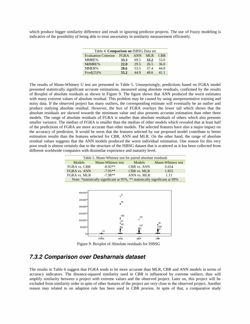
which produce bigger similarity difference and result in ignoring predictor projects. The use of Fuzzy modeling is indicative of the possibility of being able to treat uncertainty in similarity measurement efficiently.

Table 4. Comparison on ISBSG Data set Evaluation Criterion FGRA ANN MLR CBR MMRE% 33.3 69.5 33.2 53.0 MdMRE% 22.0 29.5 26.5 36.0 MMER% 28.6 53.5 37.4 44.8 Pred(25)% 55.2 44.9 48.6 41.1

The results of Mann-Whitney U test are presented in Table 5. Unsurprisingly, predictions based on FGRA model presented statistically significant accurate estimations, measured using absolute residuals, confirmed by the results of Boxplot of absolute residuals as shown in Figure 9. The figure shows that ANN produced the worst estimates with many extreme values of absolute residual. This problem may be caused by using unrepresentative training and noisy data. If the observed project has many outliers, the corresponding estimate will eventually be an outlier and produce outlying absolute residual. However, the box of FGRA overlays the lower tail which shows that the absolute residuals are skewed towards the minimum value and also presents accurate estimation than other three models. The range of absolute residuals of FGRA is smaller than absolute residuals of others which also presents smaller variance. The median of FGRA is smaller than the median of other models which revealed that at least half of the predictions of FGRA are more accurate than other models. The selected features have also a major impact on the accuracy of prediction. It would be seem that the features selected by our proposed model contribute to better estimation results than the features selected for CBR, ANN and MLR. On the other hand, the range of absolute residual values suggests that the ANN models produced the worst individual estimation. One reason for this very poor result is almost certainly due to the structure of the ISBSG dataset that is scattered as it has been collected from different worldwide companies with dissimilar experience and maturity level.

Table 5. Mann-Whitney test for paired absolute residuals Models Mann-Whitney test Models Mann-Whitney test

FGRA vs. CBR -8.92** CBR vs. ANN 0.654 FGRA vs. ANN -7.95** CBR vs. MLR 1.855 FGRA vs. MLR -7.98** ANN vs. MLR 1.11

Note: *statistically significant at 95%, ** statistically significant at 99%

Figure 9. Boxplot of Absolute residuals for ISBSG

7.3.2 Comparison over Desharnais dataset

The results in Table 6 suggest that FGRA tends to be more accurate than MLR, CBR and ANN models in terms of accuracy indicators. The distance-squared similarity used in CBR is influenced by extreme outliers, thus will amplify similarity between a project with extreme values and the observed project. Later on, this project will be excluded from similarity order in spite of other features of the project are very close to the observed project. Another reason may related to no adaption rule has been used in CBR process. In spite of that, a comparative study

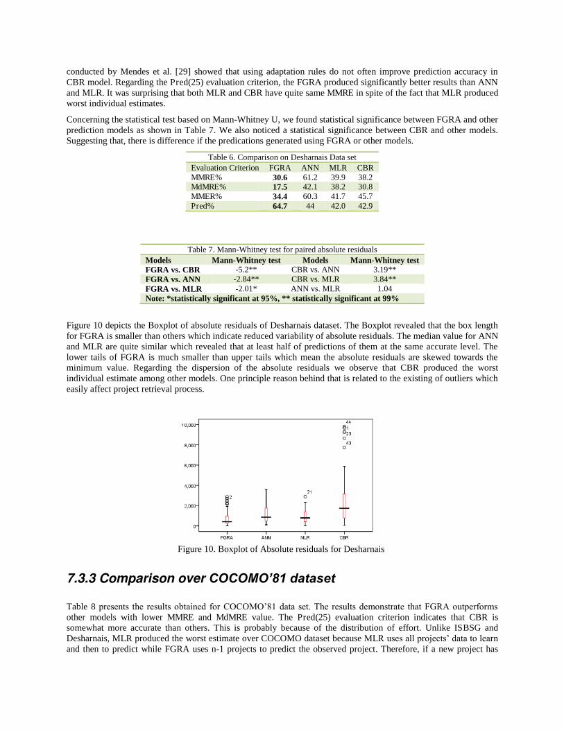
conducted by Mendes et al. [29] showed that using adaptation rules do not often improve prediction accuracy in CBR model. Regarding the Pred(25) evaluation criterion, the FGRA produced significantly better results than ANN and MLR. It was surprising that both MLR and CBR have quite same MMRE in spite of the fact that MLR produced worst individual estimates.

Concerning the statistical test based on Mann-Whitney U, we found statistical significance between FGRA and other prediction models as shown in Table 7. We also noticed a statistical significance between CBR and other models. Suggesting that, there is difference if the predications generated using FGRA or other models.

Table 6. Comparison on Desharnais Data set Evaluation Criterion FGRA ANN MLR CBR MMRE% 30.6 61.2 39.9 38.2 MdMRE% 17.5 42.1 38.2 30.8 MMER% 34.4 60.3 41.7 45.7 Pred% 64.7 44 42.0 42.9

Table 7. Mann-Whitney test for paired absolute residuals Models Mann-Whitney test Models Mann-Whitney test FGRA vs. CBR -5.2** CBR vs. ANN 3.19** FGRA vs. ANN -2.84** CBR vs. MLR 3.84** FGRA vs. MLR -2.01* ANN vs. MLR 1.04 Note: *statistically significant at 95%, ** statistically significant at 99%

Figure 10 depicts the Boxplot of absolute residuals of Desharnais dataset. The Boxplot revealed that the box length for FGRA is smaller than others which indicate reduced variability of absolute residuals. The median value for ANN and MLR are quite similar which revealed that at least half of predictions of them at the same accurate level. The lower tails of FGRA is much smaller than upper tails which mean the absolute residuals are skewed towards the minimum value. Regarding the dispersion of the absolute residuals we observe that CBR produced the worst individual estimate among other models. One principle reason behind that is related to the existing of outliers which easily affect project retrieval process.

Figure 10. Boxplot of Absolute residuals for Desharnais

7.3.3 Comparison over COCOMO’81 dataset

Table 8 presents the results obtained for COCOMO‟81 data set. The results demonstrate that FGRA outperforms other models with lower MMRE and MdMRE value. The Pred(25) evaluation criterion indicates that CBR is somewhat more accurate than others. This is probably because of the distribution of effort. Unlike ISBSG and Desharnais, MLR produced the worst estimate over COCOMO dataset because MLR uses all projects‟ data to learn and then to predict while FGRA uses n-1 projects to predict the observed project. Therefore, if a new project has

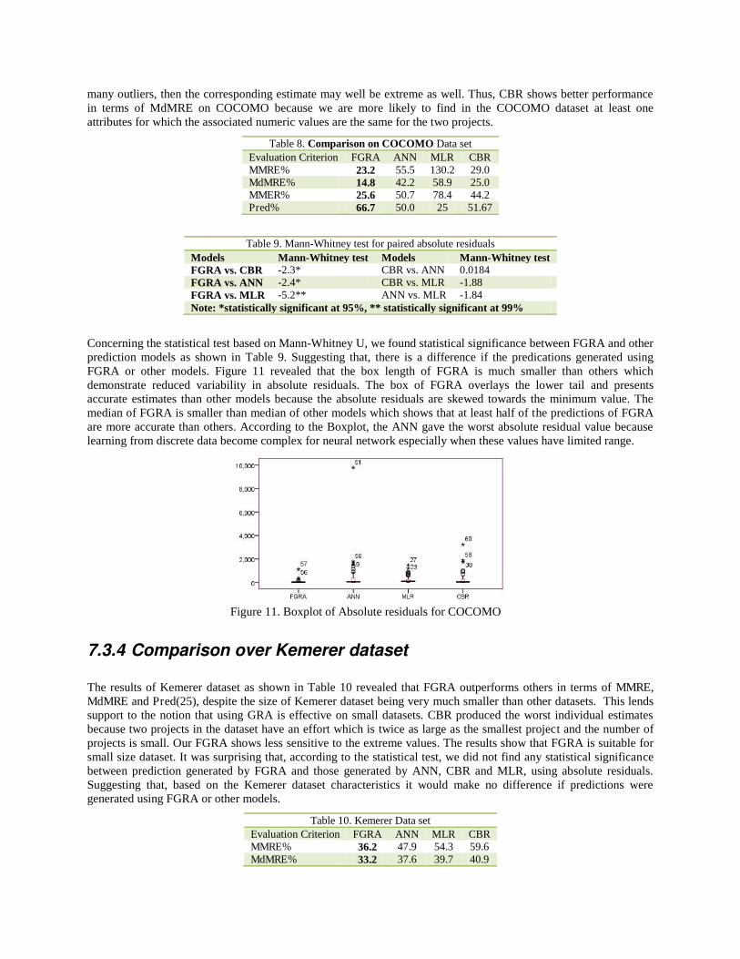
many outliers, then the corresponding estimate may well be extreme as well. Thus, CBR shows better performance in terms of MdMRE on COCOMO because we are more likely to find in the COCOMO dataset at least one attributes for which the associated numeric values are the same for the two projects.

Table 8. Comparison on COCOMO Data set Evaluation Criterion FGRA ANN MLR CBR MMRE% 23.2 55.5 130.2 29.0 MdMRE% 14.8 42.2 58.9 25.0 MMER% 25.6 50.7 78.4 44.2 Pred% 66.7 50.0 25 51.67

Table 9. Mann-Whitney test for paired absolute residuals Models Mann-Whitney test Models Mann-Whitney test FGRA vs. CBR -2.3* CBR vs. ANN 0.0184 FGRA vs. ANN -2.4* CBR vs. MLR -1.88 FGRA vs. MLR -5.2** ANN vs. MLR -1.84 Note: *statistically significant at 95%, ** statistically significant at 99%

Concerning the statistical test based on Mann-Whitney U, we found statistical significance between FGRA and other prediction models as shown in Table 9. Suggesting that, there is a difference if the predications generated using FGRA or other models. Figure 11 revealed that the box length of FGRA is much smaller than others which demonstrate reduced variability in absolute residuals. The box of FGRA overlays the lower tail and presents accurate estimates than other models because the absolute residuals are skewed towards the minimum value. The median of FGRA is smaller than median of other models which shows that at least half of the predictions of FGRA are more accurate than others. According to the Boxplot, the ANN gave the worst absolute residual value because learning from discrete data become complex for neural network especially when these values have limited range.

Figure 11. Boxplot of Absolute residuals for COCOMO

7.3.4 Comparison over Kemerer dataset

The results of Kemerer dataset as shown in Table 10 revealed that FGRA outperforms others in terms of MMRE, MdMRE and Pred(25), despite the size of Kemerer dataset being very much smaller than other datasets. This lends support to the notion that using GRA is effective on small datasets. CBR produced the worst individual estimates because two projects in the dataset have an effort which is twice as large as the smallest project and the number of projects is small. Our FGRA shows less sensitive to the extreme values. The results show that FGRA is suitable for small size dataset. It was surprising that, according to the statistical test, we did not find any statistical significance between prediction generated by FGRA and those generated by ANN, CBR and MLR, using absolute residuals. Suggesting that, based on the Kemerer dataset characteristics it would make no difference if predictions were generated using FGRA or other models.

Table 10. Kemerer Data set Evaluation Criterion FGRA ANN MLR CBR MMRE% 36.2 47.9 54.3 59.6 MdMRE% 33.2 37.6 39.7 40.9

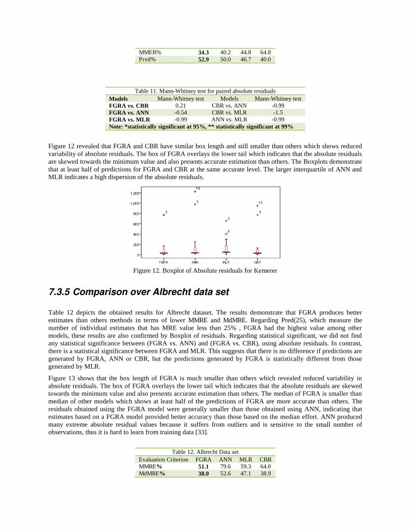
MMER% 34.3 40.2 44.8 64.8 Pred% 52.9 50.0 46.7 40.0

Table 11. Mann-Whitney test for paired absolute residuals Models Mann-Whitney test Models Mann-Whitney test FGRA vs. CBR 0.21 CBR vs. ANN -0.99 FGRA vs. ANN -0.54 CBR vs. MLR -1.5 FGRA vs. MLR -0.99 ANN vs. MLR -0.99 Note: *statistically significant at 95%, ** statistically significant at 99%

Figure 12 revealed that FGRA and CBR have similar box length and still smaller than others which shows reduced variability of absolute residuals. The box of FGRA overlays the lower tail which indicates that the absolute residuals are skewed towards the minimum value and also presents accurate estimation than others. The Boxplots demonstrate that at least half of predictions for FGRA and CBR at the same accurate level. The larger interquartile of ANN and MLR indicates a high dispersion of the absolute residuals.

Figure 12. Boxplot of Absolute residuals for Kemerer

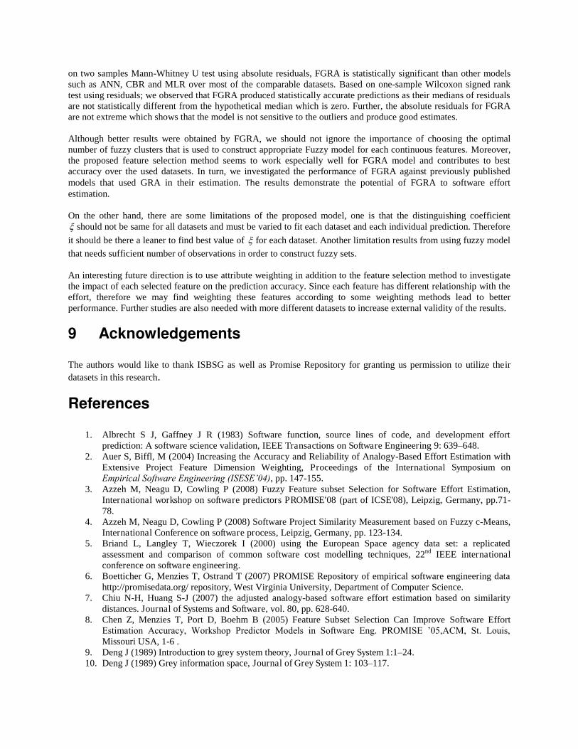
7.3.5 Comparison over Albrecht data set

Table 12 depicts the obtained results for Albrecht dataset. The results demonstrate that FGRA produces better estimates than others methods in terms of lower MMRE and MdMRE. Regarding Pred(25), which measure the number of individual estimates that has MRE value less than 25% , FGRA had the highest value among other models, these results are also confirmed by Boxplot of residuals. Regarding statistical significant, we did not find any statistical significance between (FGRA vs. ANN) and (FGRA vs. CBR), using absolute residuals. In contrast, there is a statistical significance between FGRA and MLR. This suggests that there is no difference if predictions are generated by FGRA, ANN or CBR, but the predictions generated by FGRA is statistically different from those generated by MLR.

Figure 13 shows that the box length of FGRA is much smaller than others which revealed reduced variability in absolute residuals. The box of FGRA overlays the lower tail which indicates that the absolute residuals are skewed towards the minimum value and also presents accurate estimation than others. The median of FGRA is smaller than median of other models which shows at least half of the predictions of FGRA are more accurate than others. The residuals obtained using the FGRA model were generally smaller than those obtained using ANN, indicating that estimates based on a FGRA model provided better accuracy than those based on the median effort. ANN produced many extreme absolute residual values because it suffers from outliers and is sensitive to the small number of observations, thus it is hard to learn from training data [33].

Table 12. Albrecht Data set Evaluation Criterion FGRA ANN MLR CBR MMRE% 51.1 79.6 59.3 64.0 MdMRE% 38.0 52.6 47.1 38.9

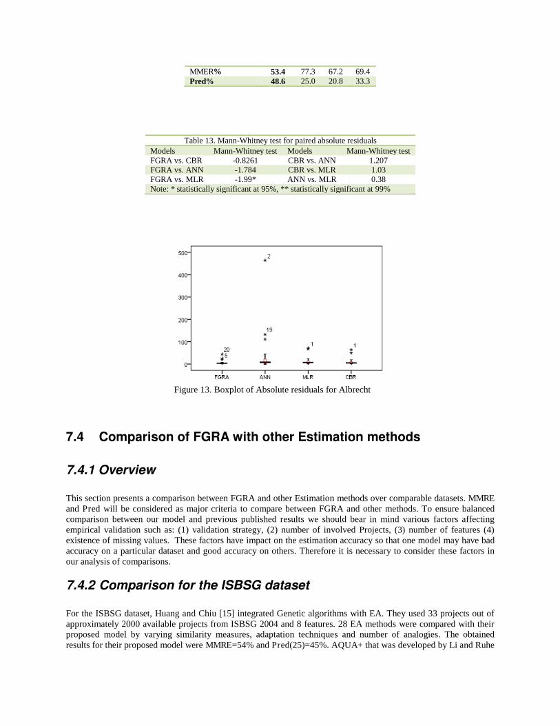
MMER% 53.4 77.3 67.2 69.4 Pred% 48.6 25.0 20.8 33.3

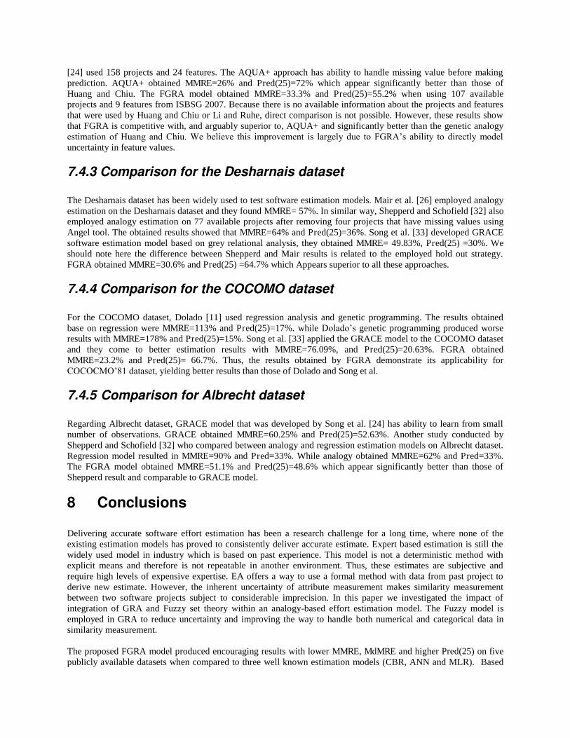
Table 13. Mann-Whitney test for paired absolute residuals Models Mann-Whitney test Models Mann-Whitney test FGRA vs. CBR -0.8261 CBR vs. ANN 1.207 FGRA vs. ANN -1.784 CBR vs. MLR 1.03 FGRA vs. MLR -1.99* ANN vs. MLR 0.38 Note: * statistically significant at 95%, ** statistically significant at 99%

Figure 13. Boxplot of Absolute residuals for Albrecht

7.4 Comparison of FGRA with other Estimation methods

7.4.1 Overview

This section presents a comparison between FGRA and other Estimation methods over comparable datasets. MMRE and Pred will be considered as major criteria to compare between FGRA and other methods. To ensure balanced comparison between our model and previous published results we should bear in mind various factors affecting empirical validation such as: (1) validation strategy, (2) number of involved Projects, (3) number of features (4) existence of missing values. These factors have impact on the estimation accuracy so that one model may have bad accuracy on a particular dataset and good accuracy on others. Therefore it is necessary to consider these factors in our analysis of comparisons.

7.4.2 Comparison for the ISBSG dataset

For the ISBSG dataset, Huang and Chiu [15] integrated Genetic algorithms with EA. They used 33 projects out of approximately 2000 available projects from ISBSG 2004 and 8 features. 28 EA methods were compared with their proposed model by varying similarity measures, adaptation techniques and number of analogies. The obtained results for their proposed model were MMRE=54% and Pred(25)=45%. AQUA+ that was developed by Li and Ruhe

[24] used 158 projects and 24 features. The AQUA+ approach has ability to handle missing value before making prediction. AQUA+ obtained MMRE=26% and Pred(25)=72% which appear significantly better than those of Huang and Chiu. The FGRA model obtained MMRE=33.3% and Pred(25)=55.2% when using 107 available projects and 9 features from ISBSG 2007. Because there is no available information about the projects and features that were used by Huang and Chiu or Li and Ruhe, direct comparison is not possible. However, these results show that FGRA is competitive with, and arguably superior to, AQUA+ and significantly better than the genetic analogy estimation of Huang and Chiu. We believe this improvement is largely due to FGRA‟s ability to directly model uncertainty in feature values.

7.4.3 Comparison for the Desharnais dataset

The Desharnais dataset has been widely used to test software estimation models. Mair et al. [26] employed analogy estimation on the Desharnais dataset and they found MMRE= 57%. In similar way, Shepperd and Schofield [32] also employed analogy estimation on 77 available projects after removing four projects that have missing values using Angel tool. The obtained results showed that MMRE=64% and Pred(25)=36%. Song et al. [33] developed GRACE software estimation model based on grey relational analysis, they obtained MMRE= 49.83%, Pred(25) =30%. We should note here the difference between Shepperd and Mair results is related to the employed hold out strategy. FGRA obtained MMRE=30.6% and Pred(25) =64.7% which Appears superior to all these approaches.

7.4.4 Comparison for the COCOMO dataset

For the COCOMO dataset, Dolado [11] used regression analysis and genetic programming. The results obtained base on regression were MMRE=113% and Pred(25)=17%. while Dolado‟s genetic programming produced worse results with MMRE=178% and Pred(25)=15%. Song et al. [33] applied the GRACE model to the COCOMO dataset and they come to better estimation results with MMRE=76.09%, and Pred(25)=20.63%. FGRA obtained MMRE=23.2% and Pred(25)= 66.7%. Thus, the results obtained by FGRA demonstrate its applicability for COCOCMO‟81 dataset, yielding better results than those of Dolado and Song et al.

7.4.5 Comparison for Albrecht dataset

Regarding Albrecht dataset, GRACE model that was developed by Song et al. [24] has ability to learn from small number of observations. GRACE obtained MMRE=60.25% and Pred(25)=52.63%. Another study conducted by Shepperd and Schofield [32] who compared between analogy and regression estimation models on Albrecht dataset. Regression model resulted in MMRE=90% and Pred=33%. While analogy obtained MMRE=62% and Pred=33%. The FGRA model obtained MMRE=51.1% and Pred(25)=48.6% which appear significantly better than those of Shepperd result and comparable to GRACE model.

8 Conclusions

Delivering accurate software effort estimation has been a research challenge for a long time, where none of the existing estimation models has proved to consistently deliver accurate estimate. Expert based estimation is still the widely used model in industry which is based on past experience. This model is not a deterministic method with explicit means and therefore is not repeatable in another environment. Thus, these estimates are subjective and require high levels of expensive expertise. EA offers a way to use a formal method with data from past project to derive new estimate. However, the inherent uncertainty of attribute measurement makes similarity measurement between two software projects subject to considerable imprecision. In this paper we investigated the impact of integration of GRA and Fuzzy set theory within an analogy-based effort estimation model. The Fuzzy model is employed in GRA to reduce uncertainty and improving the way to handle both numerical and categorical data in similarity measurement. The proposed FGRA model produced encouraging results with lower MMRE, MdMRE and higher Pred(25) on five publicly available datasets when compared to three well known estimation models (CBR, ANN and MLR). Based

on two samples Mann-Whitney U test using absolute residuals, FGRA is statistically significant than other models such as ANN, CBR and MLR over most of the comparable datasets. Based on one-sample Wilcoxon signed rank test using residuals; we observed that FGRA produced statistically accurate predictions as their medians of residuals are not statistically different from the hypothetical median which is zero. Further, the absolute residuals for FGRA are not extreme which shows that the model is not sensitive to the outliers and produce good estimates. Although better results were obtained by FGRA, we should not ignore the importance of choosing the optimal number of fuzzy clusters that is used to construct appropriate Fuzzy model for each continuous features. Moreover, the proposed feature selection method seems to work especially well for FGRA model and contributes to best accuracy over the used datasets. In turn, we investigated the performance of FGRA against previously published models that used GRA in their estimation. The results demonstrate the potential of FGRA to software effort estimation. On the other hand, there are some limitations of the proposed model, one is that the distinguishing coefficient should not be same for all datasets and must be varied to fit each dataset and each individual prediction. Therefore

it should be there a leaner to find best value of for each dataset. Another limitation results from using fuzzy model

that needs sufficient number of observations in order to construct fuzzy sets. An interesting future direction is to use attribute weighting in addition to the feature selection method to investigate the impact of each selected feature on the prediction accuracy. Since each feature has different relationship with the effort, therefore we may find weighting these features according to some weighting methods lead to better performance. Further studies are also needed with more different datasets to increase external validity of the results.

9 Acknowledgements

The authors would like to thank ISBSG as well as Promise Repository for granting us permission to utilize their datasets in this research.

References

1. Albrecht S J, Gaffney J R (1983) Software function, source lines of code, and development effort prediction: A software science validation, IEEE Transactions on Software Engineering 9: 639–648.

2. Auer S, Biffl, M (2004) Increasing the Accuracy and Reliability of Analogy-Based Effort Estimation with Extensive Project Feature Dimension Weighting, Proceedings of the International Symposium on Empirical Software Engineering (ISESE’04), pp. 147-155.

3. Azzeh M, Neagu D, Cowling P (2008) Fuzzy Feature subset Selection for Software Effort Estimation, International workshop on software predictors PROMISE'08 (part of ICSE'08), Leipzig, Germany, pp.71-78.

4. Azzeh M, Neagu D, Cowling P (2008) Software Project Similarity Measurement based on Fuzzy c-Means, International Conference on software process, Leipzig, Germany, pp. 123-134.

5. Briand L, Langley T, Wieczorek I (2000) using the European Space agency data set: a replicated assessment and comparison of common software cost modelling techniques, 22nd IEEE international conference on software engineering.

6. Boetticher G, Menzies T, Ostrand T (2007) PROMISE Repository of empirical software engineering data http://promisedata.org/ repository, West Virginia University, Department of Computer Science.

7. Chiu N-H, Huang S-J (2007) the adjusted analogy-based software effort estimation based on similarity distances. Journal of Systems and Software, vol. 80, pp. 628-640.

8. Chen Z, Menzies T, Port D, Boehm B (2005) Feature Subset Selection Can Improve Software Effort Estimation Accuracy, Workshop Predictor Models in Software Eng. PROMISE ‟05,ACM, St. Louis, Missouri USA, 1-6 .

9. Deng J (1989) Introduction to grey system theory, Journal of Grey System 1:1–24. 10. Deng J (1989) Grey information space, Journal of Grey System 1: 103–117.

11. Dolado JJ (2001) On the problem of the software cost function, Journal of Information and Software Technology 43: 61–72.

12. Haykin, S. (1999) Neural Networks: A Comprehensive Foundation, Prentice Hall, ISBN 0-13-273350-1. 13. Hsu CJ, Huang CY (2007) Improving Effort Estimation Accuracy by Weighted Grey relational Analysis

During Software development, 14th Asia-Pacific Software Engineering Conference, pp. 534-541. 14. Huang S-J, Chiu N-H, Chen L-W (2007) Integration of the grey relational analysis with genetic algorithm

for software effort estimation. European Journal of operational and research 188: 898-909. 15. Huang SJ, Chiu NH (2006) optimization of analogy weights by genetic algorithm for software effort

estimation. Journal of Information & software technology: 48 : 1034-1045 16. Idri A, Abran A, Khoshgoftaar T (2001) Fuzzy Analogy: a New Approach for Software Effort Estimation,

11th International Workshop in Software Measurements, pp. 93-101. 17. ISBSG (2007) International Software Benchmarking standards Group, Data repository release 10, web site:

http://www.isbsg.org (visited 20 August 2008). 18. Jorgensen M, Indahl U, Sjoberg D (2003), Software effort estimation by analogy and "regression toward

the mean", Journal of Systems and Software 68: 253-262. 19. Kemerer CF (1987) An empirical validation of software cost estimation models, Comm. ACM 30 : 416–

429. 20. Keung J, Kitchenham B (2008) Experiments with Analogy-X for software cost estimation, 19th Australian

Conference on software engineering, pp. 229-238. 21. Kirsopp C, Shepperd M (2002) Case and Feature Subset Selection in Case-Based Software Project Effort

Prediction, Proceedings of 22nd International Conference on Knowledge-Based Systems and Applied Artificial Intelligence (SGAI'02).

22. Kirsopp C, Shepperd MJ, Hart J (2002) Search Heuristics, Case-based Reasoning and Software Project Effort Prediction, Proceedings of the Genetic and Evolutionary Computation Conference, pp. 1367-1374.

23. Li J, Ruhe G (2008) Multi-criteria Decision Analysis for Customization of Estimation by Analogy Method AQUA+, International workshop on software predictors PROMISE'08, Leipzig, Germany, pp. 55-62.

24. Li, J, Ruhe, G (2008) Analysis of attribute weighting heuristics for analogy-based software effort estimation method AQUA+, Journal of Empirical Software Engineering 13: 63-96.

25. Liebchen G, Shepperd M (2008) Data sets and data Quality in software engineering, International workshop on software predictors PROMISE'08, Leipzig, Germany, pp. 39-44.

26. Mair C, Kadoda G, Lefley M, Phalp K, Schofield C, Shepperd M, Webster S (2000) an investigation of machine learning based prediction systems, Journal of Systems and Software 53 : 23–29.

27. Martin C L, Pasquier J L, Yanez C M, Gutierrez A T (2005) Software Development Effort Estimation Using Fuzzy Logic: A Case Study, proceeding of Sixth Mexican International Conference on Computer Science (ENC'05), pp. 113-120.

28. Mendes E, Mosley N, Counsell S (2003) A replicated assessment of the use of adaptation rules to improve Web cost estimation, International Symposium on Empirical Software Engineering, pp. 100-109.

29. Mendes E, Watson I, Triggs C, Mosley N, Counsell S (2003) A comparative study of Cost Estimation models for web hypermedia applications, Journal of Empirical Software Engineering 8:163-193.

30. Mittas N, Athanasiades M, Angelis L (2007) improving analogy-based software cost estimation by a resampling Method, Journal of Information & software technology.

31. Myrtveit I, Stensrud E (1999) A controlled experiment to assess the benefits of estimating with analogy and regression models, IEEE transactions on software engineering 25: 510-525.

32. Shepperd M J, Schofield C (1997) Estimating Software Project Effort Using Analogies, IEEE Transaction on Software Engineering 23:736-743.

33. Song Q, Shepperd M, Mair C (2005) Using Grey Relational Analysis to Predict Software Effort with Small Data Sets, Proceedings of the 11th International Symposium on Software Metrics (METRICS’05), pp. 35-45.

34. Tadayon N (2005) Neural Network Approach for Software Cost Estimation, International Conference on Information Technology: Coding and Computing (ITCC'05) - Volume II, pp. 815-818.

35. Xie X L, Beni G (1991) A validity measure for Fuzzy clustering, IEEE Transactions on Pattern Analysis Machine Intelligence 13: 841-847.

36. Xu Z, Khoshgoftaar T (2004) Identification of Fuzzy models of software effort estimation, Journal of Fuzzy Sets and Systems 145: 141-163.

37. Zadeh L (1997) Toward a theory of Fuzzy information granulation and its centrality in human reasoning and Fuzzy logic. Journal Fuzzy sets and Systems 90: 111-127.

Mohammad Y. Azzeh is a full-time PhD research student at the school of Informatics, university of Bradford. He was awarded a BSc degree in Computer Engineering from Applied Science University, Jordan in 2001. He then joined Telematix Corporation, Jordan as hardware designer. He received MSc degree in Software Engineering from university of the West of England, Bristol, United Kingdom in 2003. During mater degree he joined MOTOROLA, Swindon, U.K. as software developer for 6 months. He was working as a faculty staff member in software engineering department at Applied Science University for 4 years. His research interests included

software cost estimation, software project management. Publications include the best conference papers for International conference on software process (ICSP'08) and international workshop on software predictors (Promise'08).

Dr. Daniel Neagu is Senior Lecturer in Computing at the University of Bradford and leads the postgraduate taught programmes of the Department of Computing. He worked for the EU FP5 RTN IMAGETOX (2000-2004) and coordinated a WP within the EU FP5 QoL Integrated Project DEMETRA (2003-2006). He also coordinated 4 EPSRC and industry financed projects in the UK. Daniel leads the Machine Learning, Knowledge Representation and Data Mining Lab, part of the Emergent Computing Research Group. His research work addresses computational intelligence techniques for data quality, data mining, data fusion and information integration, automation of

knowledge discovery and applications in predictive toxicology, visual arts, software engineering, web semantics and social computing. Daniel is an invited referee for evaluation of EPSRC and The Leverhulme Trust project proposals and PC member of international conferences and journals. He authored 5 books and over 60 papers in refereed international journals and conferences. Daniel is member of IEEE - Institute of Electrical and Electronics Engineers, ACM - Association for Computing Machinery and BCS - British Computer Society. Daniel is Fellow of the Higher Education Academy and member of the University Committee for Ethics in Research.

Professor Peter Cowling received the MA and DPhil degrees from Corpus Christi College, University of Oxford, in 1989 and 1997 respectively. He is Associate Dean (Research) at the School of Informatics and co-founder and leader of the MOSAIC (Modelling Optimisation Scheduling And Intelligent Control) and BUGRD (Bradford University Games Research and Development) research centres at the University of Bradford. He was previously a Reader in the School of Computer Science at the University of Nottingham and a Senior Decision Support

Consultant at AI Systems BV and the Université Libre de Bruxelles, Belgium. Prof. Cowling led a team responsible for creating the market-leading SteelPlanner range of steel scheduling software while at A Systems BV, and is a founder and director of Cowling Scheduling Consultants Ltd. which has created scheduling decision support systems continuously over several years used to schedule personnel of the UK‟s largest financial institutions. His research and knowledge transfer work has received coverage on TV, radio, news and Internet media. His research interests are in modeling and optimization of real-world scheduling problems, evolutionary algorithms and their hybrids with exact and metaheuristic methods, hyperheuristics, and the creation of effective AI approaches for games. He has published over 70 papers in these areas, winning “best paper” prize at EvoCOP 2001. He has sat on the programme committee of over 40 conferences, and will be programme chair for EvoCOP 2009. He has given invited talks to conferences and businesses across Europe.