Embed Size (px)
Citation preview
Pergamon
PH:S0957-4158 (96) 00010-4
Mechatronics Vol. 6, No. 5, pp. 537-555, 1996 Copyright © 1996 Elsevier Science Ltd.
Printed in Great Britain. All rights reserved. 0957-4158/96 $15.00+0.00
FUZZY CONTROL STRATEGY DESIGN FOR AN AUTOPILOT ON AUTOMOBILE CHASSIS
DYNAMOMETER TEST STANDS
CHE-WUN HONG and TSON-WEI SHIO
Department of Power Mechanical Engineering, National Tsing Hua University, Hsinchu 30043, Taiwan
(Received 16 August 1995; accepted 30 January 1996)
Abstract--An optimal control strategy designed for an autopilot system to aid driving pattern simulation on automobile chassis dynamometer test stands is described. The control strategy is based on modern fuzzy theory to simulate driver behavior under dynamic road-driving conditions. Using a phase plane analysis approach, the performance characteristics of a conventional nonfuzzy proportional-integral (PI) control, a linear fuzzy control, and a nonlinear fuzzy control are compared. A devised optimal model, based on the combination of both linear and nonlinear fuzzy theories, is introduced. The validation of the effect of each model on the dynamic vehicle performance is also carded out using computer simulation. An IM 240 driving pattern is chosen as an example driving condition. The results show that the new fuzzy control strategy is able to achieve the target of fast response and high accuracy during the driving test. Hence it is adequate to be implemented into the autopilot system to replace an experienced driver in the vehicle performance laboratory. Copyright © 1996 Elsevier Science Ltd.
1. INTRODUCTION
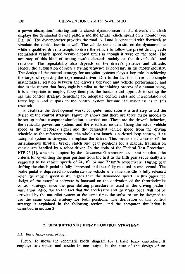
An autopilot is basically a robot driver, which is a very convenient mechatronic device which aids driving pattern tests on automobile chassis dynamometer test stands. This computer controlled robot driver makes the experiment more repeatable and more accurate, provided that a proper control strategy is chosen. Traditionally, PID (Proportional-Integral-Derivative) controls have been the favorite strategies to be employed in this industry. However, the modern fuzzy control strategy is closer to an expert system. Moreover, the fuzzy theory provides a convenient interfacing tool between human thinking and machine operation. Hence, the application of fuzzy controls in various industries is having more and more potential. This is the incentive for the research of the present paper.
Firstly, we introduce the measurement of fuel economy and emission levels of a passenger car, which is normally carded out inside a vehicle performance laboratory instead of on the proving ground. The major instruments in such a laboratory include
537
538 CHE-WUN HONG and TSON-WEI SHIO
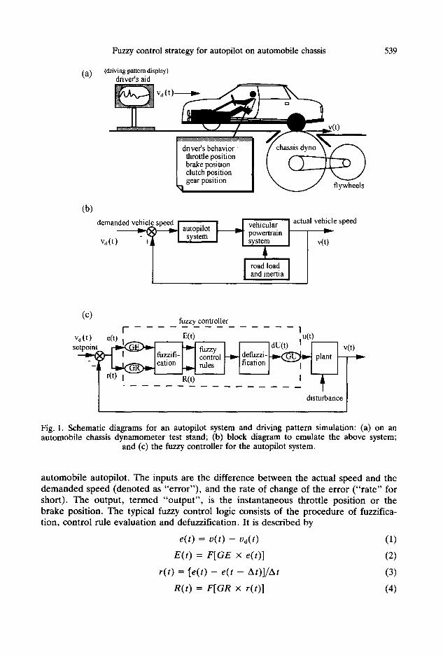
a power absorption/motoring unit, a chassis dynamometer, and a driver's aid which displays the demanded driving pattern and the actual vehicle speed on a monitor (see Fig. la). The dynamometer provides the road load and is connected with flywheels to simulate the vehicle inertia as well. The vehicle remains in situ on the dynamometer while a qualified driver attempts to drive the vehicle to follow the preset driving cycle (demanded vehicle speed versus elapsed time) as though it were on the road. The accuracy of this kind of testing results depends mainly on the driver's skill and reactions. The repeatability also depends on the driver's patience and attitude. Hence, the automation of such a testing sequence is necessary in the motor industry. The design of the control strategy for autopilot systems plays a key role in achieving the target of replacing the experienced driver. Due to the fact that there is no simple mathematical relation between the driver's behavior and vehicle performance, and due to the reason that fuzzy logic is similar to the thinking process of a human being, it is appropriate to employ fuzzy theory as the fundamental approach to set up the optimal control strategy. Searching for adequate control rules and interpretation of fuzzy inputs and outputs in the control system become the major issues in this research.
To facilitate the development work, computer simulation is a first step to aid the design of the control strategy. Figure lb shows that there are three major models to be set up before computer simulation is carried out. These are the driver's behavior, the vehicular powertrain system, and the road load models. Using the actual vehicle speed as the feedback signal and the demanded vehicle speed from the driving schedule as the reference point, the whole test bench is a closed loop control, if an autopilot system is designed to replace the driver. This means that controls of the instantaneous throttle, brake, clutch and gear positions for a manual transmission vehicle are handled by a robot driver. In the code of the Federal Test Procedure, FTP 75 [1], which is adopted by the Taiwanese Government as a test standard, the criteria for up-shifting the gear position from the first to the fifth gear sequentially are suggested to be vehicle speeds of 24, 40, 64 and 72 km/h respectively. During gear shifting the clutch pedal is fully depressed and then fully released in one second. The brake pedal is depressed to decelerate the vehicle when the throttle is fully released when the vehicle speed is still higher than the demanded speed. In this paper the design of the autopilot software is focussed on the derivation of the throttle/brake control strategy, since the gear shifting procedure is fixed in the driving pattern simulation. Also, due to the fact that the accelerator and the brake pedal will not be activated by the autopilot system at the same time, the software can be designed to use the same control strategy for both positions. The derivation of this control strategy is explained in the following section, and the computer simulation is described in section 3.
2. DESCRIPTION OF FUZZY CONTROL STRATEGY
2.1. Basic fuzzy control logic
Figure lc shows the schematic block diagram for a basic fuzzy controller. It employs two inputs and results in one output in the case of the design of an
(a)
Fuzzy control strategy for autopilot on automobile chassis
(driving pattern display) driver's aid
539
(b) demanded vehicle speed I . . . . I I ] actual vehicle speed ~ autopllot ~ vehicular
Vd(t ) -+l Isystem [ I [ p°wertrainsystemandroad ¢inertialOad '[ v(t)
(c) fuzzy controller vd(t) etO I" E(t) lu(t) setpoinl ~
disturbance
Fig. 1. Schematic diagrams for an autopilot system and driving pattern simulation: (a) on an automobile chassis dynamometer test stand; (b) block diagram to emulate the above system;
and (c) the fuzzy controller for the autopilot system.
automobile autopilot. The inputs are the difference between the actual speed and the demanded speed (denoted as "error"), and the rate of change of the error ("rate" for short). The output, termed "output", is the instantaneous throttle position or the brake position. The typical fuzzy control logic consists of the procedure of fuzzifica- tion, control rule evaluation and defuzzification. It is described by
e ( t ) = v ( t ) -- Vd(t )
E ( t ) = F [ G E x e(t)]
r ( t ) = ~e( t ) - e ( t - A t ) ] / A t
R ( t ) = F [ G R × r(t)]
(1)
(2)
(3)
(4)
540 CHE-WUN HONG and TSON-WEI SHIO
u(t) = du(t) + u(t - At) = GU x dU(t ) + u(t - At). (5)
In the above equations, t is the current time; At is the sampling time step; e(t), r(t) , v(t), vd(t) and u(t) denote the error, rate, plant output (vehicle speed), setpoint (demanded vehicle speed) and the fuzzy controller output (or plant input, such as the throttle position and the brake position) at the current time respectively; t - At stands for the sampling time at the previous step; F[ ] indicates fuzzification function. GE (gain for error) and GR (gain for rate) are scalers for adjusting the value of error and rate to be within [ -1 , +1]. GU (gain for controller output) is the scaler of the fuzzy controller output. The term du(t) designates the incremental output of the fuzzy controller at sampling time t. The fuzzy sets, E(t ) , R( t ) and dU(t) , correspond to the scaled error, the scaled rate and the defuzzified incremental output of the fuzzy controller. These are represented by " E R R O R " , " R A T E " and "OUTPUT" respect- ively.
Assuming a regular fuzzy set, the principal values of E R R O R and RATE are denoted by x[i], i = 1 . . . . . N , ordered from most negative to most positive, and centered on zero. With scaling performed externally, we require the extreme values of x[1] and x[N] to be - 1 and +1 respectively. The principal values are equally spaced in the form
x[i] = - 1 + 2(i - 1)/(N - 1), i = 1 . . . . . N. (6)
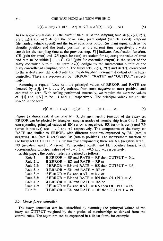
Figure 2a shows that, if we take N = 3, the membership function of the fuzzy set E R R O R can be plotted by triangles, ranging grades of membership from 0 to 1. The corresponding principal values of EN (error is negative), EZ (error is zero) and EP (error is positive) are - 1 , 0 and + 1 respectively. The components of the fuzzy set RATE are similar to ERROR, with different notations expressed by RN (rate is negative), RZ (rate is zero) and RP (rate is positive). The membership function of the fuzzy set OUTPUT in Fig. 2b has five components; these are NL (negative large), NS (negative small), Z (zero), PS (positive small) and PL (positive large), with corresponding principal values of - 1 , -0 .5 , 0, +0.5 and +1 respectively.
In this paper, the control rules are defined as follows. Rule 1: If E R R O R = EP and RATE = RP then OUTPUT = NL. Rule 2.1: If E R R O R = EZ and RATE -- RP or Rule 2.2: if E R R O R = EP and RATE -- RZ then OUTPUT = NS. Rule 3.1: If E R R O R -- EN and RATE = RP or Rule 3.2: if E R R O R -- EZ and RATE -- RZ or Rule 3.3: if E R R O R = EP and RATE -- RN then OUTPUT = Z. Rule 4.1: If E R R O R -- EN and RATE -- RZ or Rule 4.2: if E R R O R = EZ and RATE -- RN then OUTPUT = PS. Rule 5: If E R R O R = EN and RATE -- RN then OUTPUT = PL.
2.2. Linear fuzzy controller
The fuzzy controller can be defuzzified by summing the principal values of the fuzzy set OUTPUT weighted by their grades of memberships as derived from the control rules. The algorithm can be expressed in a linear form, for example
Fuzzy control strategy for autopilot on automobile chassis 541
(a)
membership
EN EZ RN RZ
EP RP
1 ERROR, RATE
(b) membership
-1 -0.5 0 0.5 1
OUTPUT
Fig. 2. Membership functions for fuzzy sets of (a) ERROR, RATE and (b) OUTPUT.
Nxr ( /1)] d t J = [m, × - 1 + , (7)
i = l t N - 1
where mi is the membership evaluated from the ith control rule. A so-called Zadeh fuzzy logic [2] is adopted to evaluate the above fuzzy control rules. The definition of the logic in mathematical form is
a AND b -- min(a , b), a OR b = max(a , b), (8)
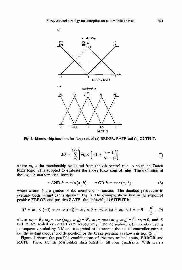
where a and b are grades of the membership function. The detailed procedure to evaluate both mi and d U is shown in Fig. 3. The example shows that in the region of positive E R R O R and positive RATE, the defuzzified OUTPUT is
E dU = m t x ( - 1 ) + m2 x (-½) + m3 x 0 + m4 x (1) + m5 x 1 = - R
2 (9)
w h e r e m I = R , m 2 = m a x ( m 2 1 , m 2 2 ) = E , m 4 = m a x ( m 4 1 , m 4 2 ) = 0 , m5 = 0 , a n d E and R are scaled error and rate respectively. The derivative, d U, so obtained is subsequently scaled by GU and integrated to determine the actual controller output, i.e. the instantaneous throttle position or the brake position as shown in Eqn (5).
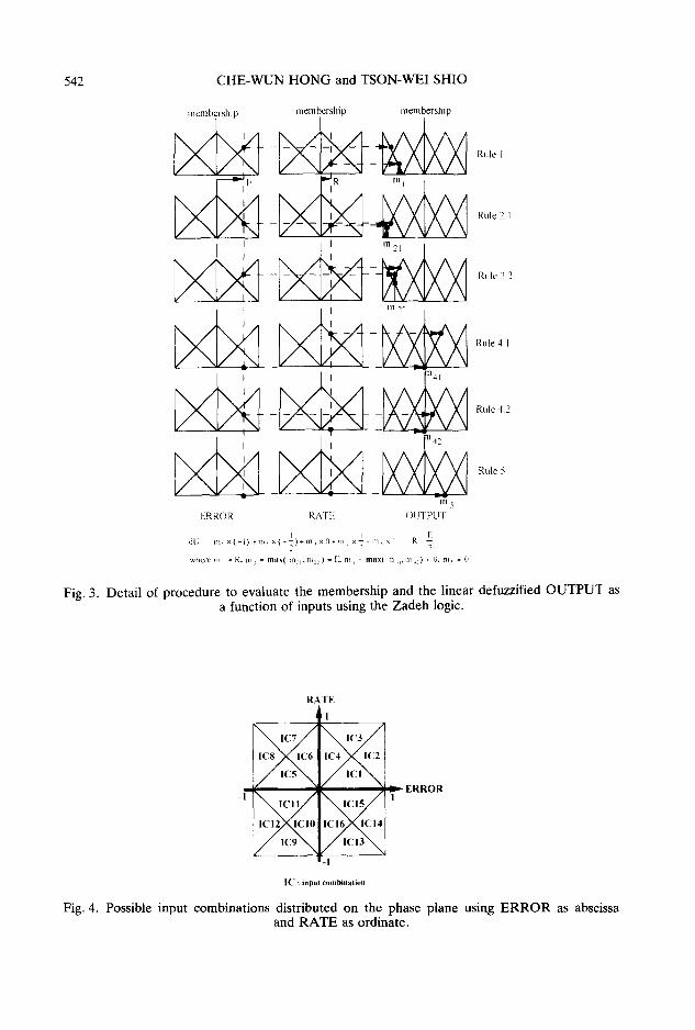
Figure 4 shows the possible combinations of the two scaled inputs, E R R O R and RATE. There are 16 possibilities distributed in all four quadrants. With scalers
542 CHE-WUN HONG and TSON-WEI SHIO
membership meinbership menlbership
' t ' ,n:, /
1 l 111 2 2
3"
m 5
ERROR RA[E ()UTPUT
' R E dl~] ~ n 1 1 × { I ) + I I 1 2 × { ) + [11 ~ × 0 + n ] 4 × ~ ' + h i s × i = q
, * h e I e m ! = R . m : = Il l l . lx{ I I ' I l l 2 ' ) = [ i 1114 = m a x ( Il l H Ill 4~ ) = U , I l l • = ()
Rule I
Rule 2 1
Rule _.~
Rule 4 1
Rule 4 2
Rule 5
Fig. 3. Detail of procedure to evaluate the membership and the linear defuzzified OUTPUT as a function of inputs using the Zadeh logic.
R A T E
I
[C : input combinalion
Fig. 4. Possible input combinations distributed on the phase plane using ERROR as abscissa and RATE as ordinate.
Fuzzy control strategy for autopilot on automobile chassis 543
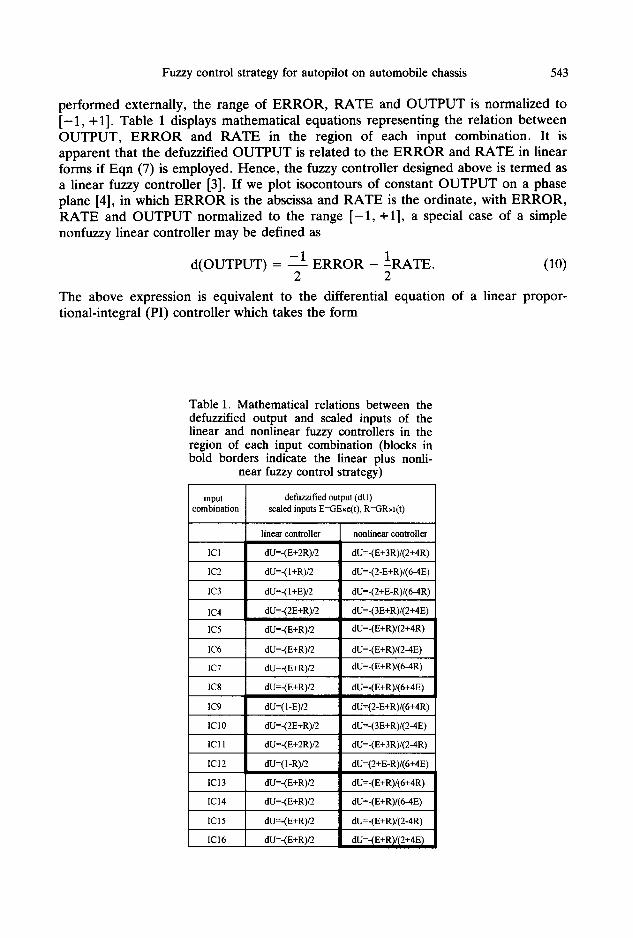
performed externally, the range of ERROR, RATE and OUTPUT is normalized to [ -1 , +1]. Table 1 displays mathematical equations representing the relation between OUTPUT, ERROR and RATE in the region of each input combination. It is apparent that the defuzzified OUTPUT is related to the ERROR and RATE in linear forms if Eqn (7) is employed. Hence, the fuzzy controller designed above is termed as a linear fuzzy controller [3]. If we plot isocontours of constant OUTPUT on a phase plane [4], in which ERROR is the abscissa and RATE is the ordinate, with ERROR, RATE and OUTPUT normalized to the range [ -1 , +1], a special case of a simple nonfuzzy linear controller may be defined as
d(OUTPUT) = - 1 ERROR - 1RATE. (10) 2 2
The above expression is equivalent to the differential equation of a linear propor- tional-integral (PI) controller which takes the form
Table 1. Mathematical relations between the defuzzified output and scaled inputs of the linear and nonlinear fuzzy controllers in the region of each input combination (blocks in bold borders indicate the linear plus nonli-
near fuzzy control strategy)
input defuzzified output (dU) combination scaled inputs E=GExe(t), R=GRxI(t)
nonlinear controller
ICI
1C2 dU=-(1 +R)/2
IC3 dU=-(I+E)/2
IC4
linear controller
dU=-(E+2R)/2
IC5
IC6 dU=-(E+R)/2
IC7 dU=-(E+R)/2
IC8
IC9
dU=-(2E+R)/2
dU=-(E+R)/2
dU=-(E+R)/2
dU=(1-E)/2
IC 10 dU=-(2E+R)/2
ICI 1 dU=-(E+2R)/2
IC12 dU=( 1 -R)~
dU=-(E+R)/2 1C13
IC14 dU=-(E+R)/2
IC 15 dU=-(E+R)/2
IC16 dU=-(E+R)/2
dU=-(E+3R)/(2+4R)
dU=-(2-E+R)/(6-4E)
dU=-(2+E-R)/(6-4R)
dU=-(3E+R)/(2+4E)
dU~(E+R)/(2+4R)
dU=-(E+R)/(2-4E)
dU=-(E+R)/(6-4R)
dU=-(E+R)/(6+4E)
dU=(2-E+R)/(6+4R)
dU=-(3E+R)/(2-4E)
dU=-(E+3R)/(2-4R)
dU=(2+E-R)/(6+4E)
dU=-(E+R)/(6+4R)
dU=-(E+R)/(6-4E)
dU=-(E+R)/(2-4R)
dU=-(E+R)/(2+4E)
544 CHE-WUN HONG and TSON-WEI SHIO
du dv - - - k i ( v - s) - kp , (11) dt dt
where s is the setpoint; ki, ke designate the gain constants for the integral controller and the proportional controller respectively.
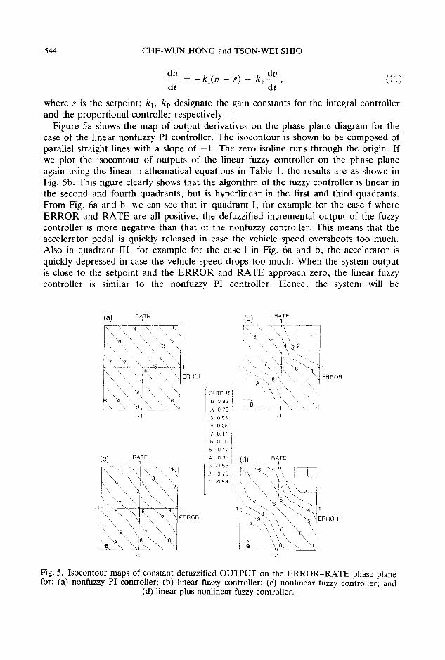
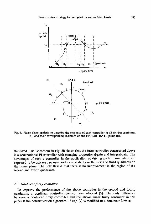
Figure 5a shows the map of output derivatives on the phase plane diagram for the case of the linear nonfuzzy PI controller. The isocontour is shown to be composed of parallel straight lines with a slope of -1 . The zero isoline runs through the origin. If we plot the isocontour of outputs of the linear fuzzy controller on the phase plane again using the linear mathematical equations in Table 1, the results are as shown in Fig. 5b. This figure clearly shows that the algorithm of the fuzzy controller is linear in the second and fourth quadrants, but is hyperlinear in the first and third quadrants. From Fig. 6a and b, we can see that in quadrant I, for example for the case f where ERROR and RATE are all positive, the defuzzified incremental output of the fuzzy controller is more negative than that of the nonfuzzy controller. This means that the accelerator pedal is quickly released in case the vehicle speed overshoots too much. Also in quadrant III, for example for the case 1 in Fig. 6a and b, the accelerator is quickly depressed in case the vehicle speed drops too much. When the system output is close to the setpoint and the ERROR and RATE approach zero, the linear fuzzy controller is similar to the nonfuzzy PI controller. Hence, the system will be
(a) RATE 1
1 1
ERROR
l \ "\ "',6!'7 " "'i ""A "s:.\ "i', " , , ""6 1
1
(C) RATE 1
J \ \ ".. \ \ \ ,, [ % .\ ] . 3. .,.'
\",\ \ \ \ s i \ \ \ \ l \ \ "\7 " . \ / ' \ . \ \ ~
' x \ / \ 5 \1
\\'~\ \ \ 9 k \ - - ' \ , ]8 " ~ . " 6 /
1
I
ERROR
(b) RATE 1
, . , , 4 ' 3 2
1~ ~ - - ~" "~S "~4 1 ! ...... " " , " , \ , ! ERROR
4", ~, " \, 7 OUTPUr i ' , , 7 "
o.aB I ~ " " ~" "" 6 ] B ', \ . . ji
A 0 7 0 : . . . . . . . . . . . . . . . i ~, 9 0 5 3 i 1 8 035 7 017 6 0 0 0 , 5 -017 1 4 -0351 3 -0 53 i (d) RATE1
2 -o7o l i 1 .o 88 !
J
I
ERROR
Fig. 5. Isocontour maps of constant defuzzified OUTPUT on the E R R O R - R A T E phase plane for: (a) nonfuzzy PI controller; (b) linear fuzzy controller; (c) nonlinear fuzzy controller; and
(d) linear plus nonlinear fuzzy controller.
Fuzzy control strategy for autopilot on automobile chassis 545
(a)
vehicle speed
V d
; i (case) ; , , I I ~ 1 h I I I I I
, ~ ~ i ~ t I I I I I e V _ _ 1 1 I _ / N K ' l n . l l l ~
. . . . . . . . . r . . . . . . . 7 . . . . . . ~
t i i i i i i L i
C i i / ' , i I I I I I
b
,1, 7 elapsed time
(b) RATE (quadrant)
I11 t " I
"',,,
~ ERROR
III I ~ , IVI
I IV 2
Fig. 6. Phase plane analysis to describe the response of each controller in all driving conditions (a), and their corresponding locations on the ERROR-RATE plane (b).
stabilized. The isocontour in Fig. 5b shows that the fuzzy controller constructed above is a conventional PI controller with changing proportional-gain and integral-gain. The advantages of such a controller in the application of driving pattern simulation are expected to be quicker response and more stability in the first and third quadrants on the phase plane. The only flaw is that there is no improvement in the region of the second and fourth quadrants,
2.3. Nonlinear fuzzy controller
To improve the performance of the above controller in the second and fourth quadrants, a nonlinear controller concept was adopted [5]. The only difference between a nonlinear fuzzy controller and the above linear fuzzy controller in this paper is the defuzzification algorithm. If Eqn (7) is modified to a nonlinear form as
546 CHE-WUN HONG and TSON-WEI SHIO
/11) ] E[mi× -1+ N dU = , (12)
2 N - 1
~ m~ i = l
the relations between the defuzzified output and those scaled inputs in all four quadrants can be re-calculated and are displayed in Table 1. This table shows that the defuzzification algorithm makes the mathematical relations between the output and inputs become nonlinear in all circumstances. The output characteristics of this nonlinear fuzzy controller are plotted in Fig. 5c. The isocontour map indicates that in quadrant 112, such as case b in Fig. 6a and b, the nonlinear fuzzy controller tends to slowly accelerate the vehicle compared with the nonfuzzy PI controller. When the vehicle speed reaches case d in quadrant 111, the accelerator is then slowly released. The same control strategy is also applied in quadrants IVI and IV2, for example cases h, i and j; the vehicle speed is expected to drop to the target speed smoothly. This kind of control strategy tends to make the vehicle accelerate or decelerate smoothly without over-enriching the fuel injection system. Hence, the vehicle performance is expected to lead to greater fuel economy and smoother driving. Consequently, a second conclusion can be drawn at this stage, that the nonlinear fuzzy controller shows better performance for the cases in the second and fourth quadrants from the phase plane analysis. The only flaw appears in the cases of 1, 2, A and B in Fig. 5c, which show the wrong tendency if the same control strategy is applied in these regions.
2.4. Linear plus nonlinear fuzzy controller
To combine the advantages of both the linear and nonlinear controllers, without their inherent flaws, a new control strategy is required. We can combine the part of the linear fuzzy controller in the first and third quadrants with the part of the nonlinear fuzzy controller in the second and fourth quadrants. The detailed mathe- matical relations of this new strategy are displayed in Table 1 (see blocks with bold borders). The output characteristics of this new strategy on the phase plane are shown in Fig. 5d. It is obvious that the new strategy has been manipulated to be a linear plus nonlinear controller. The effect of this new fuzzy controller on the vehicle perform- ance will be studied in the next section.
In the above examples, we concentrate on the throttle control. For the case of brake control, the speed error is always positive, and the rate is either positive or negative. Positive rate occurs when accelerating along a downhill slope by gravity force, while negative rate is the situation when the accelerator is fully released to decelerate the vehicle but the vehicle speed is still higher than the demanded speed. Hence, these conditions fall in the region of the first and fourth quadrants as explained in Fig. 6. Since the brake control has exactly the reverse effect on the vehicle speed to that of the throttle, the incremental output of the original map has to change the sign (from negative to positive or from positive to negative) in the software. Hence, the same control strategy can still be applied but the sign of the derivative output is changed. The effects of the control strategies proposed above on vehicle performance are validated using computer simulation in the following section.
Fuzzy control strategy for autopilot on automobile chassis 547
3. COMPUTER SIMULATION
3.1. Chassis dynamometer simulation
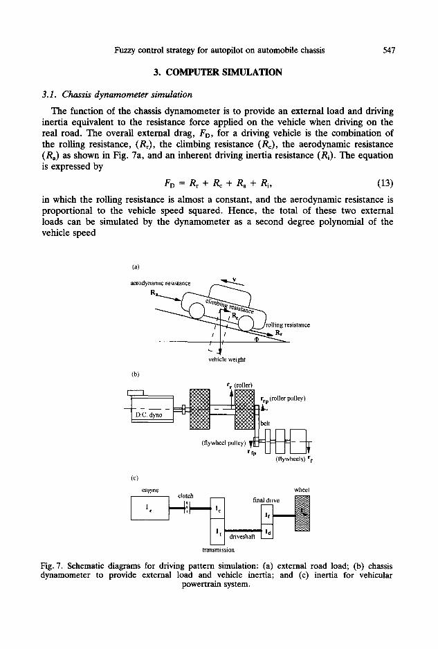
The function of the chassis dynamometer is to provide an external load and driving inertia equivalent to the resistance force applied on the vehicle when driving on the real road. The overall external drag, FD, for a driving vehicle is the combination of the rolling resistance, (Rr), the climbing resistance (Re), the aerodynamic resistance (Ra) as shown in Fig. 7a, and an inherent driving inertia resistance (Ri). The equation is expressed by
FD = Rr + Rc + Ra + Ri, (13)
in which the rolling resistance is almost a constant, and the aerodynamic resistance is proportional to the vehicle speed squared. Hence, the total of these two external loads can be simulated by the dynamometer as a second degree polynomial of the vehicle speed
(a)
aerodynamic resistance
R ~ r o l l i n g resistance
vehicle weight
(b) r r (roller)
' ~ belt
(flywheel p u ~ r fp L I L ~ I ~ T
(flywheels) r t
(c) engine wheel
clutch
I e ',
i driveshafi
transmission
Fig. 7. Schematic diagrams for driving pattern simulation: (a) external road load; (b) chassis dynamometer to provide external load and vehicle inertia; and (c) inertia for vehicular
powertrain system.
548 CHE-WUN HONG and TSON-WEI SHIO
FD, = Rr + Ra = a + c " o 2, (14)
where a and c are coefficients which are normally obtained experimentally from a coast-down test on a level road [6].
The most important term is the inertia resistance which is an additional drag (or propulsion force) when the vehicle is accelerating (or decelerating). It is normally simulated by a set of flywheels in the chassis dynamometer test bed as shown in Fig. 7b. Assuming that the tension force of the rubber belt on the roller side is exactly same as that on the flywheel side, the following relation can be derived:
m m (r i (rft 2 \ r fp / \ rr]
This means that the vehicle mass (m) can be simulated by proper choice of the flywheel mass (mf) and proper relations between radii of the roller pulley (r~p), the flywheel pulley (rfp), flywheels (rf) and rollers (rr). Hence, the chassis dynamometer is able to provide an additional inertia force or drag as
_ rrp r f dv FD2 = Ri = lmf . (16)
2 \rrp/ \ r r / dt
The climbing resistance can be simulated by a simple calculation as
FD3 = Rc = _+m" g" sin tp, (17)
where tp is the incfination angle of the road slope; + and - indicate uphill and downhill conditions. In summary, the overall external drag provided by the chassis dynamometer is
FD = FD, + FD 2 + FD3. (18)
This can be designed through an electronic control loop.
3.2. Vehicular powertrain simulation
The powertrain system in this paper includes the powerplant, i.e. the engine, and the drivetrain system. The engine performance simulator is basically a cycle simula- tion program with additional flow, thermal, and mechanical inertia submodels [7]. The in-cylinder thermo-fluid-combustion dynamics are the major processes to produce the instantaneous engine power. The ignition timing and the equivalence ratio are two of the main control parameters which influence the combustion process. These two parameters are normally controlled by an electronic control unit (ECU) which is built inside the vehicle. The other major control parameter is the throttle position, which is controlled by the driver (or the autopilot system in this paper) through a linkage from the accelerator pedal. The engine simulator was expanded to be an automotive dynamic performance simulator through combination with driveline sub-models [8]. The torque produced by the engine is transmitted to drive-wheels through the clutch, the transmission, the driveshaft, and the final drive for a manual transmission vehicle as shown in Fig. 7c. The torque ratio (CTR) through the clutch is defined to be
Fuzzy control strategy for autopilot on automobile chassis 549
CaR -- re -- 1 Xe(t) - Xft, (19) % 1 - Xft
where r e and r~ stand for the engine developed torque and the dutch output torque; X¢(t) denotes the instantaneous clutch position; and Xn represents the free travel clearance. When the clutch pedal is fully released, or X¢ <~ Xft, the torque ratio is assumed to be equal to unity. Then the angular acceleration (0 in rad/s 2) of the driveline system at the input shaft of the transmission is
0 - ~* - ~ (20) Ie + I1'
in which the equivalent inertia of the load part (see Fig. 7c) can be evaluated from the balance of rotary kinetic energy along the driveline system, i.e.
I, = Ic +-~t[It + Id +-~f(If + Iw)], (21)
where I and G denote mechanical inertia and gear ratio. Subscripts e, 1, c, t, d, f and w represent engine, load part, dutch, transmission, driveshaft, final drive and wheels respectively. The equivalent road load torque on the input shaft of the transmission is
(FD + Fb)" rw'r/d r~ = , (22)
Gt" Gf
where rw is the effective tire radius; ~d is the overall efficiency of the driveline system; Fd is the external drag provided by the dynamometer; and Fb is the brake force. The brake force is a function of the instantaneous brake position, Xb(t). It is assumed to be
Fb Xb(t) -- Xbc - Fbm~x, (23)
1 -- Xbc
where Fb,,, is the maximum brake force, Xbc is the brake pedal clearance and Xb(t ) denotes the instantaneous brake position which is decided by the fuzzy controller. When Xb ~< Xb¢, the brake force is set to be zero.
The angular velocity (0 in rad/s) of the input shaft of the transmission can be integrated from Eqn (20) using a trapezoidal method. Finally, the instantaneous vehicle speed, in km/h, is thus calculated by
r w • v(t) = 3 . 6 - - . (24) Gt" Gf
In summary, the instantaneous vehicle speed is basically a function of the instanta- neous throttle, brake, clutch and gear positions controlled by the autopilot system.
3.3. Driving pattern simulation In order to validate the effect of control strategies on the road vehicle performance,
dynamic simulation of the whole system under driving pattern conditions was carried out. A passenger car, named Arex, designed by Yue-Loong Motor Co. in Taiwan, was chosen as the baseline vehicle. This is an 1800 cc, electronic fuel injection and
550 CHE-WUN HONG and TSON-WEI SHIO
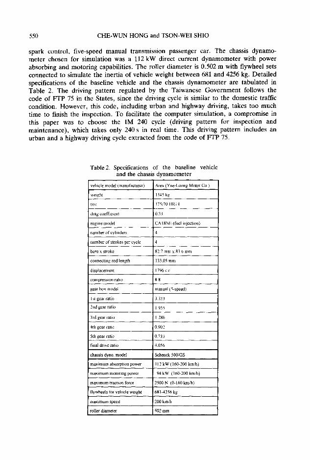
spark control, five-speed manual transmission passenger car. The chassis dynamo- meter chosen for simulation was a 112 kW direct current dynamometer with power absorbing and motoring capabilities. The roller diameter is 0.502 m with flywheel sets connected to simulate the inertia of vehicle weight between 681 and 4256 kg. Detailed specifications of the baseline vehicle and the chassis dynamometer are tabulated in Table 2. The driving pattern regulated by the Taiwanese Government follows the code of FFP 75 in the States, since the driving cycle is similar to the domestic traffic condition. However, this code, including urban and highway driving, takes too much time to finish the inspection. To facilitate the computer simulation, a compromise in this paper was to choose the IM 240 cycle (driving pattern for inspection and maintenance), which takes only 240 s in real time. This driving pattern includes an urban and a highway driving cycle extracted from the code of FTP 75.
Table 2. Specifications of the baseline vehicle and the chassis dynamometer
vehicle model (manufacturer) Arex (Yue-Loong Motor Co.)
I weight 1545 kg
tire 175/70 HRI4
drag coefficient 0.33
engine model CA I8NE (fuel injection)
number of cylinders 4
number of strokes per cycle 4
bore x stroke 827 mmx 83.6 mm
connecting rod length 13305 mm
displacemen! 1796 c.c
compression ratio 88
gear box model manual (5-speed)
I st gear ratio 3.333
2nd gear ratio 1.955
3rd gear ratio 1.286
4th gear ratio 0902
5th gear ratio 0733
final drive ratio 4.056
chassis dyno. model Schenck 500/GS
max0num absorption power 112 kW (160-200 km/h)
maximum motoring power 94 kW (160-200 km/h)
maximum traction three 2500 N (0-160 kin/h)
flywheels for vehicle weight 681-4256 kg
maximum speed 200 km/h
roller diameter 502 mm
Fuzzy control strategy for autopilot on automobile chassis 551
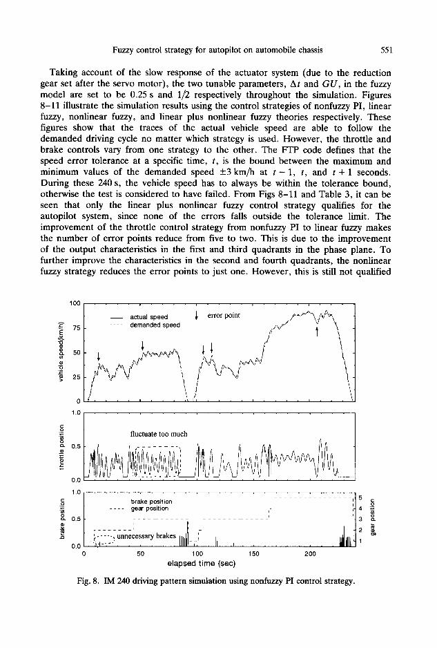
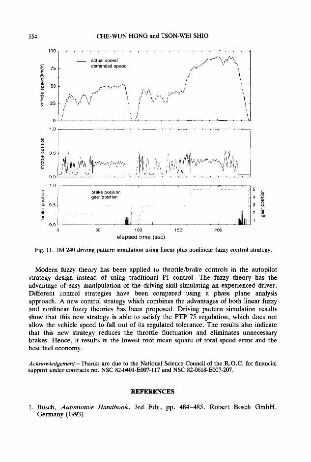
Taking account of the slow response of the actuator system (due to the reduction gear set after the servo motor), the two tunable parameters, At and GU, in the fuzzy model are set to be 0.25 s and 1//2 respectively throughout the simulation. Figures 8-11 illustrate the simulation results using the control strategies of nonfuzzy PI, linear fuzzy, nonlinear fuzzy, and linear plus nonlinear fuzzy theories respectively. These figures show that the traces of the actual vehicle speed are able to follow the demanded driving cycle no matter which strategy is used. However, the throttle and brake controls vary from one strategy to the other. The FTP code defines that the speed error tolerance at a specific time, t, is the bound between the maximum and minimum values of the demanded speed _+3 km/h at t - 1, t, and t + 1 seconds. During these 240 s, the vehicle speed has to always be within the tolerance bound, otherwise the test is considered to have failed. From Figs 8-11 and Table 3, it can be seen that only the linear plus nonlinear fuzzy control strategy qualifies for the autopilot system, since none of the errors falls outside the tolerance limit. The improvement of the throttle control strategy from nonfuzzy PI to linear fuzzy makes the number of error points reduce from five to two. This is due to the improvement of the output characteristics in the first and third quadrants in the phase plane. To further improve the characteristics in the second and fourth quadrants, the nonlinear fuzzy strategy reduces the error points to just one. However, this is still not qualified
100
J ~ ~. 75 v
~ 5o
} 2 5
0
1.0
actual speed ~ error point . . F ' ~ . . . . demanded speed
~ I , . = i i , i i i I , ,
Q- 0.5 o
0.0
1.0
ca- 0.5
0.0
fluctuate too much
. . . . L . . . . L . . . . i . . . . i , , ,
. . . . , . . . . . . . . . , . . . . . . . . .
- - brake position i ,, 5 1 . . . . gear position ," 't 4 :~
' t - - - , 3 o .
~ .... . , unnecessary brakes : . ~ - . . t . , - , V . . . . . . I1111~1-,-. . lb. .~ . . . . . . . . . lllH1 ~
0 50 1 O0 150 2 O0
elapsed time (sec)
Fig. 8. IM 240 driving pattern simulation using nonfuzzy PI control strategy.
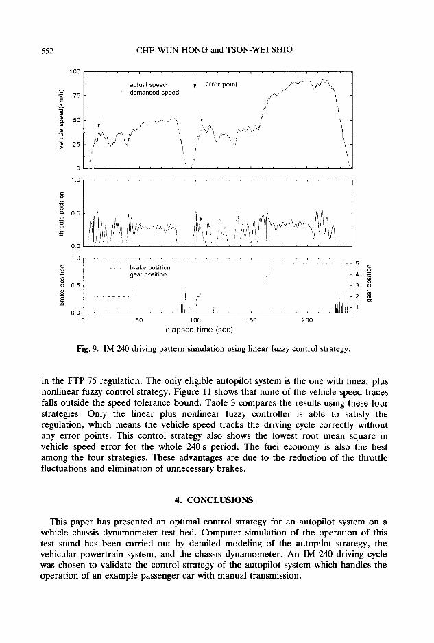
552 CHE-WUN HONG and TSON-WEI SHIO
100
o~
75
50
25
0
1.0
- - actual speed ~ error point / ~ ~ , demanded speed
\ /
~, y,,~ y ' ', ,;\ih . . . . >:.-z,j~/ 1 I V "~'d ~ 1 ,;? ~k/"'\ !'
, j , c!, I '! ,,s / :i
t
, t
o_ 0.5
0.0
1.0
o. 0.5
J ~
brake position gear position
i ,
: . . . . . lil "ll . it . . . . . . . . . . 0.0 0 50 100 150 200
elapsed t ime (sec)
5 ~_
i 4 o~ 3 o .
2 t3~
Ui i 1
Fig. 9. IM 240 driving pattern simulation using linear fuzzy control strategy.
in the FTP 75 regulation. The only eligible autopilot system is the one with linear plus nonlinear fuzzy control strategy. Figure 11 shows that none of the vehicle speed traces falls outside the speed tolerance bound. Table 3 compares the results using these four strategies. Only the linear plus nonlinear fuzzy controller is able to satisfy the regulation, which means the vehicle speed tracks the driving cycle correctly without any error points. This control strategy also shows the lowest root mean square in vehicle speed error for the whole 240 s period. The fuel economy is also the best among the four strategies. These advantages are due to the reduction of the throttle fluctuations and elimination of unnecessary brakes.
4. CONCLUSIONS
This paper has presented an optimal control strategy for an autopilot system on a vehicle chassis dynamometer test bed. Computer simulation of the operation of this test stand has been carded out by detailed modeling of the autopilot strategy, the vehicular powertrain system, and the chassis dynamometer. An IM 240 driving cycle was chosen to validate the control strategy of the autopilot system which handles the operation of an example passenger car with manual transmission.
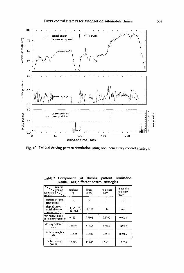
2"
t / )
0 , )
" F
1 O0
75
50
25
1.0
Fuzzy control strategy for autopilot on automobile chassis
. . . . i . . . . i . . . . i . . . . ¢ • • •
actual speed ~, i l o r point . . . . demanded speed
t l . . i i I i i • - i . . i
553
0.5
0.0
1.0
o. 0.5
.,3
0.0
brake position [ . . . . . . . . . J' 5
- - - gear position [[[t "~ 1~ Jilt L~t'L 4 "~-.~-- " - - - H - [ ' ' - . . . . . . . . ' : a i
1 - ' . . . . . . . . - - . lit . . . . . . . . . . .
50 1 O0 150 2 O0
elapsed time (sec)
Fig. 10. IM 240 driving pattern simulation using nonlinear fuzzy control strategy.
Table 3. Comparison of driving pattern simulation results using different control strategies
~,, , , control "",,~trat egy
simulation~,~ results
number of speed error points elapsed time at which tile error
root metal square of total error (km/h
nonfuzzy Pl
14,53,107, 114,208
linear fuzzy
nonlinear fuzzy
linear plus nonlinear fuzzy
0.1201
driving distance 3165.9 3159.6 3167.7 3166.5 ( I n )
fuel consumption (1) 0.2524 0.2507 0.2513 0.2506
fuel economy 12.543 12,603 12.605 12.636 (km/I)
2 I 0
14, 107 114 none
0.1002 0.1000 0.0954
554 CHE-WUN HONG and TSON-WEI SHIO
1 O0
v
o )
Q )
75
50
25
0 1.0
actual speed ~ l ..... demanded speed
o_ =
o_ 0 . 5 a)
0 . 0 ,v,j u i.,, _ J # /
1 .0 • , . . . . , . . . . , . • •
- i i ~3 gear position 4 i~ i i iJltJ f ' ,3
' , ,
0.0 " • . . . . . . . . . . . 0 50 1 O0 150 200
elapsed time (sec)
Fig. 11. IM 240 driving pattern simulation using linear plus nonlinear fuzzy control strategy.
Modern fuzzy theory has been applied to throttle/brake controls in the autopilot strategy design instead of using traditional PI control. The fuzzy theory has the advantage of easy manipulation of the driving skill simulating an experienced driver. Different control strategies have been compared using a phase plane analysis approach. A new control strategy which combines the advantages of both linear fuzzy and nonlinear fuzzy theories has been proposed. Driving pattern simulation results show that this new strategy is able to satisfy the FTP 75 regulation, which does not allow the vehicle speed to fall out of its regulated tolerance. The results also indicate that this new strategy reduces the throttle fluctuation and eliminates unnecessary brakes. Hence, it results in the lowest root mean square of total speed error and the best fuel economy.
Acknowledgement--Thanks are due to the National Science Council of the R.O.C. for financial support under contracts no. NSC 82-0401-E007-117 and NSC 82-0618-E007-207.
REFERENCES
1. Bosch, Automotive Handbook, 3rd Edn, pp. 484-485. Robert Bosch GmbH, Germany (1993).
Fuzzy control strategy for autopilot on automobile chassis 555
2. Zadeh L. A., Fuzzy sets. Inf. Control 8,338-353 (1965). 3. Siler W. and Ying H., Fuzzy control theory: the linear case. Fuzzy Sets Syst. 33,
275-290 (1989). 4. Harrison H. L. and Bollinger J. G., Introduction to Automatic Controls, 2nd Edn,
pp. 337-343. International Textbook Co. (1969). 5. Buckley J. J., Siler W. and Ying H., Fuzzy control theory: a nonlinear case.
Automatica 26,513-520 (1990). 6. Lucas G. G., Road Vehicle Performance, pp. 24-30. Gordon & Breach, New
York (1986). 7. Hong C. W., A PC-based computer simulation package for spark ignition engine
system design. Proc. I. Mech. E., Comput. Engine Technol. C430/069, 127-134 (1991).
8. Hong C. W., An automotive dynamic performance simulator for vehicular powertrain system design. Int. J. Vehicle Des. 16,264-281 (1995).