Fuzziness and Funds Allocation in Portfolio Optimization

Jack Allen1, Sukanto Bhattacharya2, Florentin Smarandache3

1 School of Accounting and Finance, Griffith University, Queensland, Australia

2 School of Information Technology, Bond University, Queensland, Australia

3 Department of Mathematics, University of New Mexico, Gallup, USA

Abstract.

Each individual investor is different, with different financial goals, different levels of

risk tolerance and different personal preferences. From the point of view of investment

management, these characteristics are often defined as objectives and constraints.

Objectives can be the type of return being sought, while constraints include factors such

as time horizon, how liquid the investor is, any personal tax situation and how risk is

handled. It’s really a balancing act between risk and return with each investor having

unique requirements, as well as a unique financial outlook – essentially a constrained

utility maximization objective. To analyze how well a customer fits into a particular

investor class, one investment house has even designed a structured questionnaire with

about two-dozen questions that each has to be answered with values from 1 to 5. The

questions range from personal background (age, marital state, number of children, job

type, education type, etc.) to what the customer expects from an investment (capital

protection, tax shelter, liquid assets, etc.). A fuzzy logic system has been designed for the

2

evaluation of the answers to the above questions. We have investigated the notion of

fuzziness with respect to funds allocation.

2000 MSC: 94D05, 03B52

Introduction.

In this paper we have designed our fuzzy system so that customers are classified to

belong to any one of the following three categories: 1

*Conservative and security-oriented (risk shy)

*Growth-oriented and dynamic (risk neutral)

*Chance-oriented and progressive (risk happy)

Besides being useful for clients, investor classification has benefits for the professional

investment consultants as well. Most brokerage houses would value this information as it

gives them a way of targeting clients with a range of financial products more effectively -

including insurance, saving schemes, mutual funds, and so forth. Overall, many

responsible brokerage houses realize that if they provide an effective service that is

tailored to individual needs, in the long-term there is far more chance that they will retain

their clients no matter whether the market is up or down.

Yet, though it may be true that investors can be categorized according to a limited

number of types based on theories of personality already in the psychological profession's

armory, it must be said that these classification systems based on the Behavioral Sciences

are still very much in their infancy and they may still suffer from the problem of their

meanings being similar to other related typographies, as well as of greatly

oversimplifying the different investor behaviors. 2

3

(I.1) Exploring the implications of utility theory on investor classification.

In our present work, we have used the familiar framework of neo-classical utility theory

to try and devise a structured system for investor classification according to the utility

preferences of individual investors (and also possible re-ordering of such preferences).

The theory of consumer behavior in modern microeconomics is entirely founded on

observable utility preferences, rejecting hedonistic and introspective aspects of utility.

According to modern utility theory, utility is a representation of a set of mutually

consistent choices and not an explanation of a choice. The basic approach is to ask an

individual to reveal his or her personal utility preference and not to elicit any numerical

measure. [1] However, the projections of the consequences of the options that we face and

the subsequent choices that we make are shaped by our memories of past experiences –

that “mind’s eye sees the future through the light filtered by the past”. However, this

memory often tends to be rather selective. [9] An investor who allocates a large portion of

his or funds to the risky asset in period t-1 and makes a significant gain will perhaps be

induced to put an even larger portion of the available funds in the risky asset in period t.

So this investor may be said to have displayed a very weak risk-aversion attitude up to

period t, his or her actions being mainly determined by past happenings one-period back.

There are two interpretations of utility – normative and positive. Normative utility

contends that optimal decisions do not always reflect the best decisions, as maximization

of instant utility based on selective memory may not necessarily imply maximization of

total utility. This is true in many cases, especially in the areas of health economics and

social choice theory. However, since we will be applying utility theory to the very

4

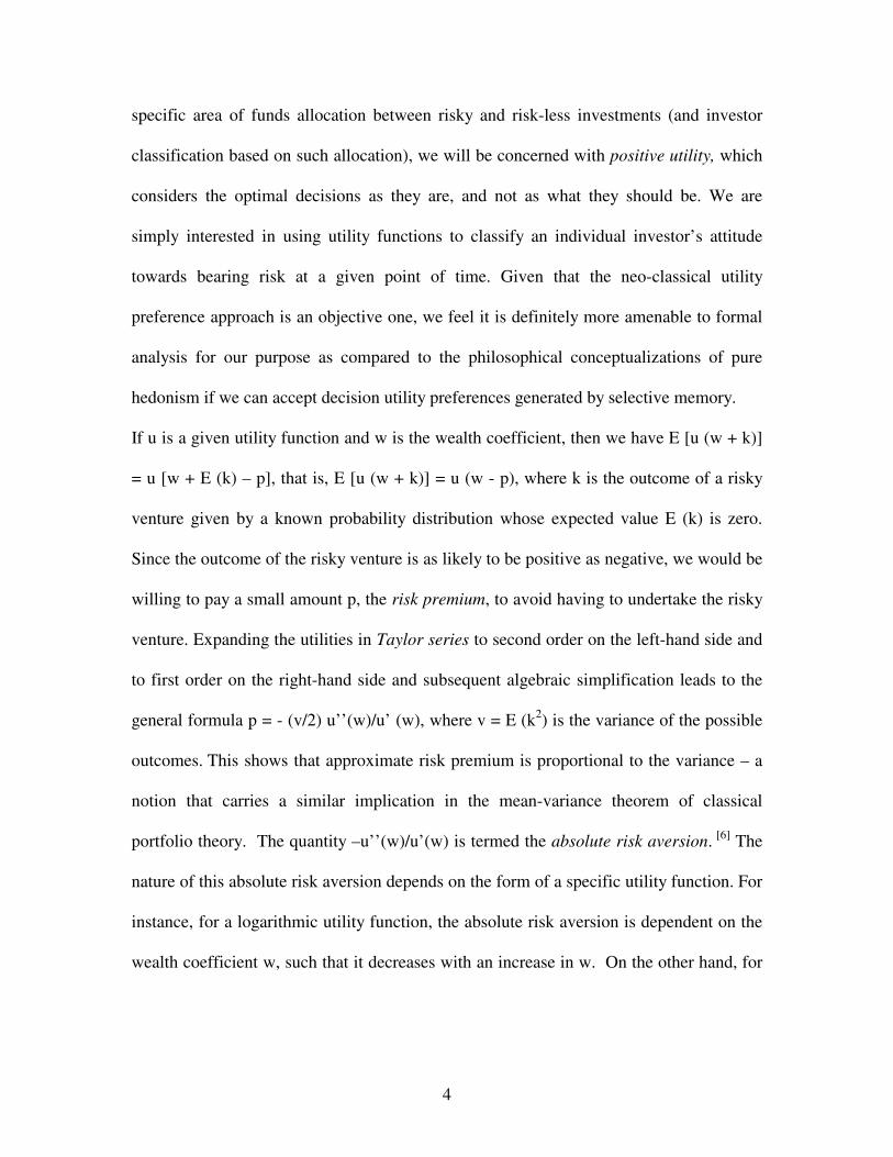
specific area of funds allocation between risky and risk-less investments (and investor

classification based on such allocation), we will be concerned with positive utility, which

considers the optimal decisions as they are, and not as what they should be. We are

simply interested in using utility functions to classify an individual investor’s attitude

towards bearing risk at a given point of time. Given that the neo-classical utility

preference approach is an objective one, we feel it is definitely more amenable to formal

analysis for our purpose as compared to the philosophical conceptualizations of pure

hedonism if we can accept decision utility preferences generated by selective memory.

If u is a given utility function and w is the wealth coefficient, then we have E [u (w + k)]

= u [w + E (k) – p], that is, E [u (w + k)] = u (w - p), where k is the outcome of a risky

venture given by a known probability distribution whose expected value E (k) is zero.

Since the outcome of the risky venture is as likely to be positive as negative, we would be

willing to pay a small amount p, the risk premium, to avoid having to undertake the risky

venture. Expanding the utilities in Taylor series to second order on the left-hand side and

to first order on the right-hand side and subsequent algebraic simplification leads to the

general formula p = - (v/2) u’’(w)/u’ (w), where v = E (k2) is the variance of the possible

outcomes. This shows that approximate risk premium is proportional to the variance – a

notion that carries a similar implication in the mean-variance theorem of classical

portfolio theory. The quantity –u’’(w)/u’(w) is termed the absolute risk aversion. [6] The

nature of this absolute risk aversion depends on the form of a specific utility function. For

instance, for a logarithmic utility function, the absolute risk aversion is dependent on the

wealth coefficient w, such that it decreases with an increase in w. On the other hand, for

5

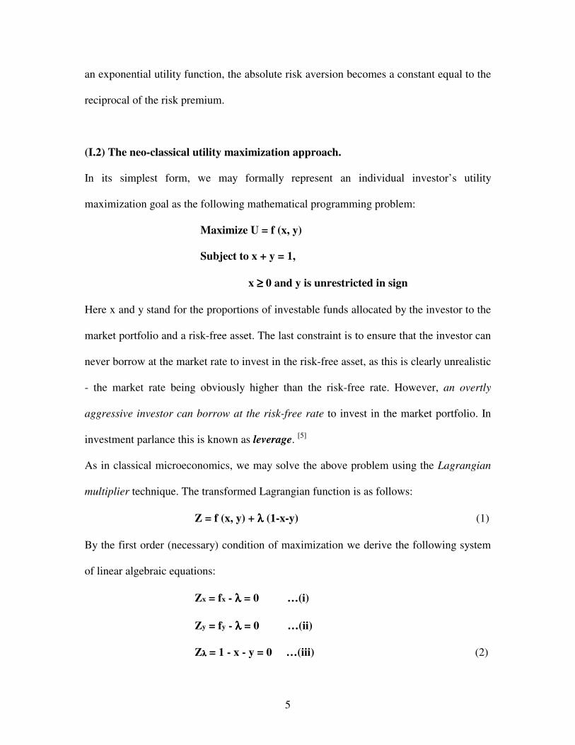
an exponential utility function, the absolute risk aversion becomes a constant equal to the

reciprocal of the risk premium.

(I.2) The neo-classical utility maximization approach.

In its simplest form, we may formally represent an individual investor’s utility

maximization goal as the following mathematical programming problem:

Maximize U = f (x, y)

Subject to x + y = 1,

x ≥≥≥≥ 0 and y is unrestricted in sign

Here x and y stand for the proportions of investable funds allocated by the investor to the

market portfolio and a risk-free asset. The last constraint is to ensure that the investor can

never borrow at the market rate to invest in the risk-free asset, as this is clearly unrealistic

- the market rate being obviously higher than the risk-free rate. However, an overtly

aggressive investor can borrow at the risk-free rate to invest in the market portfolio. In

investment parlance this is known as leverage. [5]

As in classical microeconomics, we may solve the above problem using the Lagrangian

multiplier technique. The transformed Lagrangian function is as follows:

Z = f (x, y) + λλλλ (1-x-y) (1)

By the first order (necessary) condition of maximization we derive the following system

of linear algebraic equations:

Zx = fx - λλλλ = 0 …(i)

Zy = fy - λλλλ = 0 …(ii)

Zλλλλ = 1 - x - y = 0 …(iii) (2)

6

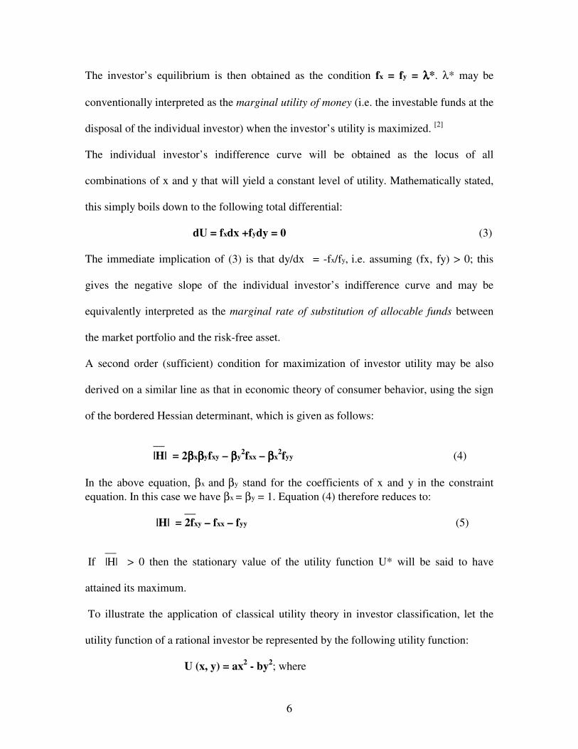
The investor’s equilibrium is then obtained as the condition fx = fy = λλλλ*. λ* may be

conventionally interpreted as the marginal utility of money (i.e. the investable funds at the

disposal of the individual investor) when the investor’s utility is maximized. [2]

The individual investor’s indifference curve will be obtained as the locus of all

combinations of x and y that will yield a constant level of utility. Mathematically stated,

this simply boils down to the following total differential:

dU = fxdx +fydy = 0 (3)

The immediate implication of (3) is that dy/dx = -fx/fy, i.e. assuming (fx, fy) > 0; this

gives the negative slope of the individual investor’s indifference curve and may be

equivalently interpreted as the marginal rate of substitution of allocable funds between

the market portfolio and the risk-free asset.

A second order (sufficient) condition for maximization of investor utility may be also

derived on a similar line as that in economic theory of consumer behavior, using the sign

of the bordered Hessian determinant, which is given as follows:

__ |H| = 2ββββxββββyfxy – ββββy

2fxx – ββββx2fyy (4)

In the above equation, βx and βy stand for the coefficients of x and y in the constraint equation. In this case we have βx = βy = 1. Equation (4) therefore reduces to: __ |H| = 2fxy – fxx – fyy (5) __ If |H| > 0 then the stationary value of the utility function U* will be said to have

attained its maximum.

To illustrate the application of classical utility theory in investor classification, let the

utility function of a rational investor be represented by the following utility function:

U (x, y) = ax2 - by2; where

7

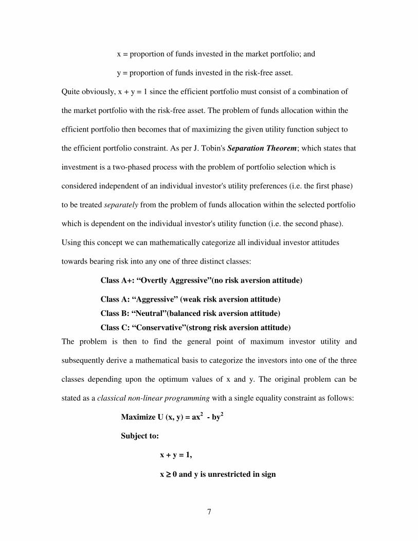
x = proportion of funds invested in the market portfolio; and

y = proportion of funds invested in the risk-free asset.

Quite obviously, x + y = 1 since the efficient portfolio must consist of a combination of

the market portfolio with the risk-free asset. The problem of funds allocation within the

efficient portfolio then becomes that of maximizing the given utility function subject to

the efficient portfolio constraint. As per J. Tobin's Separation Theorem; which states that

investment is a two-phased process with the problem of portfolio selection which is

considered independent of an individual investor's utility preferences (i.e. the first phase)

to be treated separately from the problem of funds allocation within the selected portfolio

which is dependent on the individual investor's utility function (i.e. the second phase).

Using this concept we can mathematically categorize all individual investor attitudes

towards bearing risk into any one of three distinct classes:

Class A+: “Overtly Aggressive”(no risk aversion attitude)

Class A: “Aggressive” (weak risk aversion attitude)

Class B: “Neutral”(balanced risk aversion attitude)

Class C: “Conservative”(strong risk aversion attitude)

The problem is then to find the general point of maximum investor utility and

subsequently derive a mathematical basis to categorize the investors into one of the three

classes depending upon the optimum values of x and y. The original problem can be

stated as a classical non-linear programming with a single equality constraint as follows:

Maximize U (x, y) = ax2 - by2

Subject to:

x + y = 1,

x ≥≥≥≥ 0 and y is unrestricted in sign

8

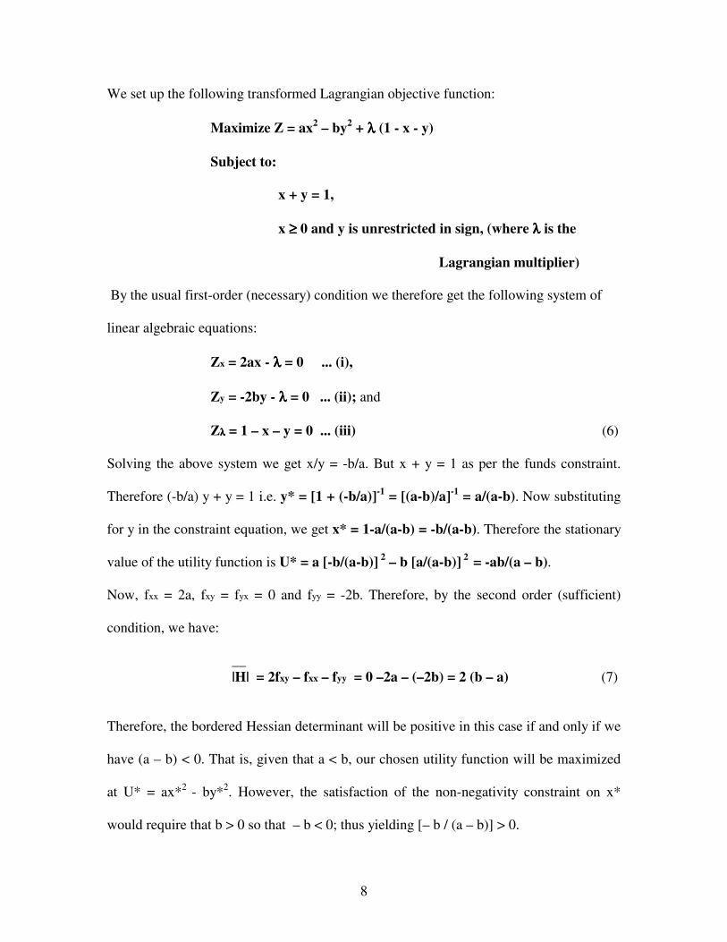
We set up the following transformed Lagrangian objective function:

Maximize Z = ax2 – by2 + λλλλ (1 - x - y)

Subject to:

x + y = 1,

x ≥≥≥≥ 0 and y is unrestricted in sign, (where λλλλ is the

Lagrangian multiplier)

By the usual first-order (necessary) condition we therefore get the following system of

linear algebraic equations:

Zx = 2ax - λλλλ = 0 ... (i),

Zy = -2by - λλλλ = 0 ... (ii); and

Zλλλλ = 1 – x – y = 0 ... (iii) (6)

Solving the above system we get x/y = -b/a. But x + y = 1 as per the funds constraint.

Therefore (-b/a) y + y = 1 i.e. y* = [1 + (-b/a)]-1 = [(a-b)/a]-1 = a/(a-b). Now substituting

for y in the constraint equation, we get x* = 1-a/(a-b) = -b/(a-b). Therefore the stationary

value of the utility function is U* = a [-b/(a-b)] 2 – b [a/(a-b)] 2 = -ab/(a – b).

Now, fxx = 2a, fxy = fyx = 0 and fyy = -2b. Therefore, by the second order (sufficient)

condition, we have:

__ |H| = 2fxy – fxx – fyy = 0 –2a – (–2b) = 2 (b – a) (7)

Therefore, the bordered Hessian determinant will be positive in this case if and only if we

have (a – b) < 0. That is, given that a < b, our chosen utility function will be maximized

at U* = ax*2 - by*2. However, the satisfaction of the non-negativity constraint on x*

would require that b > 0 so that – b < 0; thus yielding [– b / (a – b)] > 0.

9

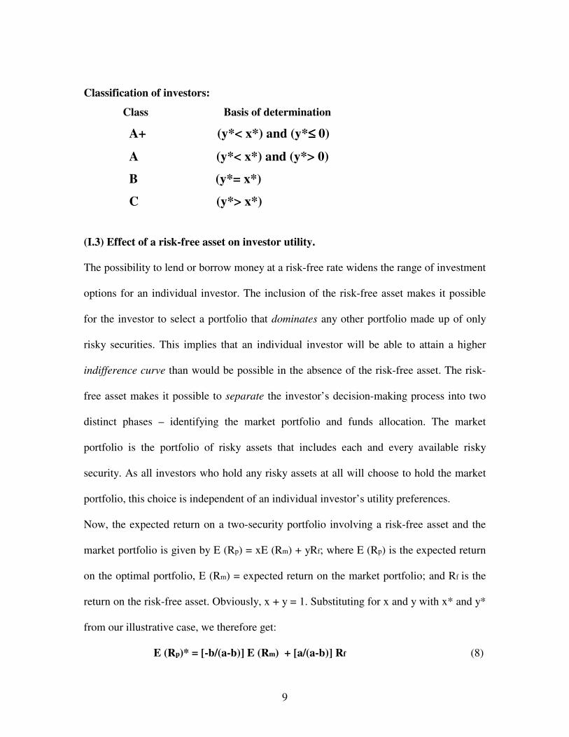
Classification of investors:

Class Basis of determination

A+ (y*< x*) and (y*≤≤≤≤ 0)

A (y*< x*) and (y*> 0)

B (y*= x*)

C (y*> x*)

(I.3) Effect of a risk-free asset on investor utility.

The possibility to lend or borrow money at a risk-free rate widens the range of investment

options for an individual investor. The inclusion of the risk-free asset makes it possible

for the investor to select a portfolio that dominates any other portfolio made up of only

risky securities. This implies that an individual investor will be able to attain a higher

indifference curve than would be possible in the absence of the risk-free asset. The risk-

free asset makes it possible to separate the investor’s decision-making process into two

distinct phases – identifying the market portfolio and funds allocation. The market

portfolio is the portfolio of risky assets that includes each and every available risky

security. As all investors who hold any risky assets at all will choose to hold the market

portfolio, this choice is independent of an individual investor’s utility preferences.

Now, the expected return on a two-security portfolio involving a risk-free asset and the

market portfolio is given by E (Rp) = xE (Rm) + yRf; where E (Rp) is the expected return

on the optimal portfolio, E (Rm) = expected return on the market portfolio; and Rf is the

return on the risk-free asset. Obviously, x + y = 1. Substituting for x and y with x* and y*

from our illustrative case, we therefore get:

E (Rp)* = [-b/(a-b)] E (Rm) + [a/(a-b)] Rf (8)

10

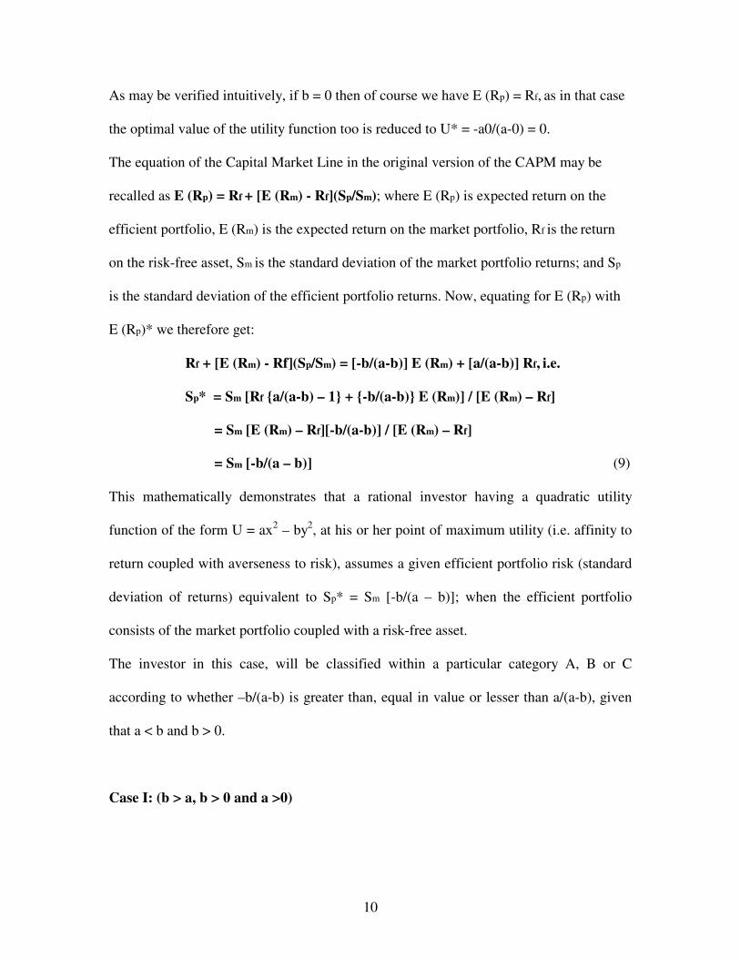
As may be verified intuitively, if b = 0 then of course we have E (Rp) = Rf, as in that case

the optimal value of the utility function too is reduced to U* = -a0/(a-0) = 0.

The equation of the Capital Market Line in the original version of the CAPM may be

recalled as E (Rp) = Rf + [E (Rm) - Rf](Sp/Sm); where E (Rp) is expected return on the

efficient portfolio, E (Rm) is the expected return on the market portfolio, Rf is the return

on the risk-free asset, Sm is the standard deviation of the market portfolio returns; and Sp

is the standard deviation of the efficient portfolio returns. Now, equating for E (Rp) with

E (Rp)* we therefore get:

Rf + [E (Rm) - Rf](Sp/Sm) = [-b/(a-b)] E (Rm) + [a/(a-b)] Rf, i.e.

Sp* = Sm [Rf {a/(a-b) – 1} + {-b/(a-b)} E (Rm)] / [E (Rm) – Rf]

= Sm [E (Rm) – Rf][-b/(a-b)] / [E (Rm) – Rf]

= Sm [-b/(a – b)] (9)

This mathematically demonstrates that a rational investor having a quadratic utility

function of the form U = ax2 – by2, at his or her point of maximum utility (i.e. affinity to

return coupled with averseness to risk), assumes a given efficient portfolio risk (standard

deviation of returns) equivalent to Sp* = Sm [-b/(a – b)]; when the efficient portfolio

consists of the market portfolio coupled with a risk-free asset.

The investor in this case, will be classified within a particular category A, B or C

according to whether –b/(a-b) is greater than, equal in value or lesser than a/(a-b), given

that a < b and b > 0.

Case I: (b > a, b > 0 and a >0)

11

Let b = 3 and a = 2. Thus, we have (b > a) and (-b < a). Then we have x* = -3/(2-3) = 3

and y* = 2/(2-3) = -2. Therefore (x*>y*) and (y*<0). So the investor can be classified as

Class A+.

Case II: (b > a, b > 0, a < 0 and b > |a|)

Let b = 3 and a = - 2. Thus, we have (b > a) and (- b < a). Then, x* = -3/(-2-3) = 0.60 and

y* = -2/(-2-3) = 0.40. Therefore (x* > y*) and (y*>0). So the investor can be re-classified

as Class A!

Case III: (b > a, b > 0, a < 0 and b = |a|)

Let b = 3 and a = -3. Thus, we have (b > a) and (b = |a|). Then we have x* = -3/(-3-3) =

0.5 and y* = -3/(-3-3) = 0.5. Therefore we have (x* = y*). So now the investor can be re-

classified as Class B!

Case IV: (b > a, b > 0, a < 0 and b < |a|)

Let b = 3 and a = -5. Thus, we have (b>a) and (b<|a|). Then we have x* = -3/(-5-3) =

0.375 and y* = -5/(-5-3) = 0.625. Therefore we have (x* < y*). So, now the investor can

be re-classified as Class C!

So we may see that even for this relatively simple utility function, the final classification

of the investor permanently into any one risk-class would be unrealistic as the range of

values for the coefficients a and b could be switching dynamically from one range to

another as the investor tries to adjust and re-adjust his or her risk-bearing attitude. This

makes the neo-classical approach insufficient in itself to arrive at a classification. Here

lies the justification to bring in a complimentary fuzzy modeling approach. Moreover, if

we bring in time itself as an independent variable into the utility maximization

framework, then one choice variable (weighted in favour of risk-avoidance) could be

12

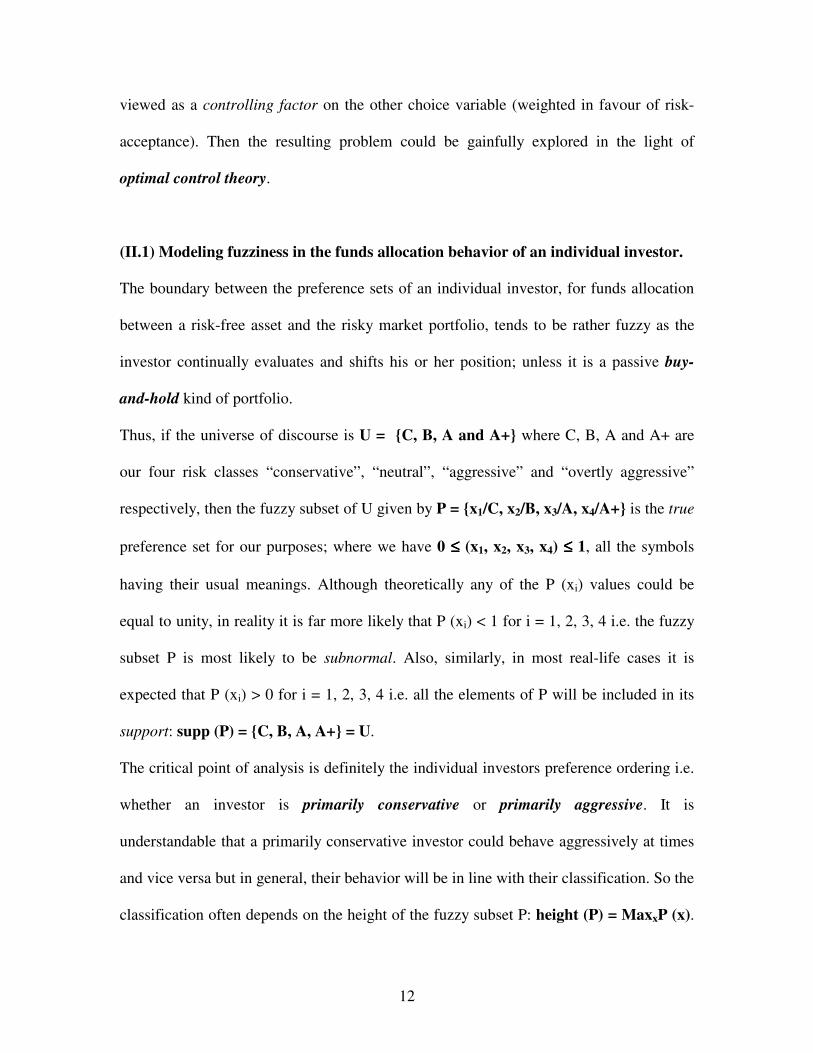
viewed as a controlling factor on the other choice variable (weighted in favour of risk-

acceptance). Then the resulting problem could be gainfully explored in the light of

optimal control theory.

(II.1) Modeling fuzziness in the funds allocation behavior of an individual investor.

The boundary between the preference sets of an individual investor, for funds allocation

between a risk-free asset and the risky market portfolio, tends to be rather fuzzy as the

investor continually evaluates and shifts his or her position; unless it is a passive buy-

and-hold kind of portfolio.

Thus, if the universe of discourse is U = {C, B, A and A+} where C, B, A and A+ are

our four risk classes “conservative”, “neutral”, “aggressive” and “overtly aggressive”

respectively, then the fuzzy subset of U given by P = {x1/C, x2/B, x3/A, x4/A+} is the true

preference set for our purposes; where we have 0 ≤≤≤≤ (x1, x2, x3, x4) ≤≤≤≤ 1, all the symbols

having their usual meanings. Although theoretically any of the P (xi) values could be

equal to unity, in reality it is far more likely that P (xi) < 1 for i = 1, 2, 3, 4 i.e. the fuzzy

subset P is most likely to be subnormal. Also, similarly, in most real-life cases it is

expected that P (xi) > 0 for i = 1, 2, 3, 4 i.e. all the elements of P will be included in its

support: supp (P) = {C, B, A, A+} = U.

The critical point of analysis is definitely the individual investors preference ordering i.e.

whether an investor is primarily conservative or primarily aggressive. It is

understandable that a primarily conservative investor could behave aggressively at times

and vice versa but in general, their behavior will be in line with their classification. So the

classification often depends on the height of the fuzzy subset P: height (P) = MaxxP (x).

13

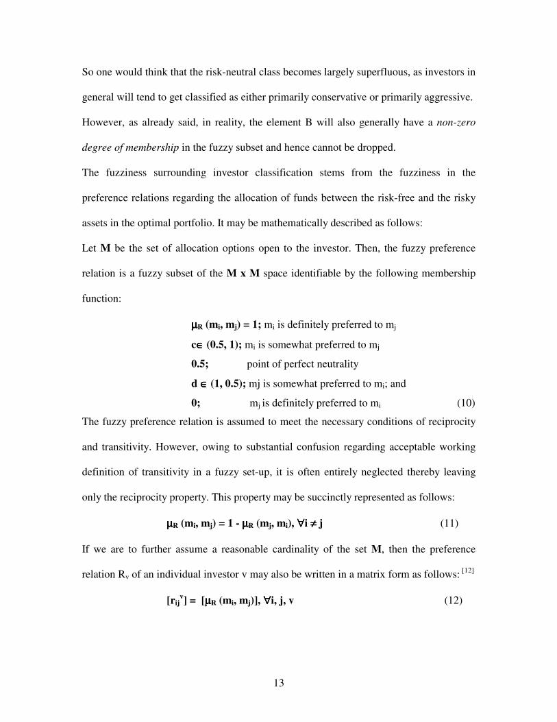
So one would think that the risk-neutral class becomes largely superfluous, as investors in

general will tend to get classified as either primarily conservative or primarily aggressive.

However, as already said, in reality, the element B will also generally have a non-zero

degree of membership in the fuzzy subset and hence cannot be dropped.

The fuzziness surrounding investor classification stems from the fuzziness in the

preference relations regarding the allocation of funds between the risk-free and the risky

assets in the optimal portfolio. It may be mathematically described as follows:

Let M be the set of allocation options open to the investor. Then, the fuzzy preference

relation is a fuzzy subset of the M x M space identifiable by the following membership

function:

µµµµR (mi, mj) = 1; mi is definitely preferred to mj

c∈∈∈∈ (0.5, 1); mi is somewhat preferred to mj

0.5; point of perfect neutrality

d ∈∈∈∈ (1, 0.5); mj is somewhat preferred to mi; and

0; mj is definitely preferred to mi (10)

The fuzzy preference relation is assumed to meet the necessary conditions of reciprocity

and transitivity. However, owing to substantial confusion regarding acceptable working

definition of transitivity in a fuzzy set-up, it is often entirely neglected thereby leaving

only the reciprocity property. This property may be succinctly represented as follows:

µµµµR (mi, mj) = 1 - µµµµR (mj, mi), ∀∀∀∀i ≠≠≠≠ j (11)

If we are to further assume a reasonable cardinality of the set M, then the preference

relation Rv of an individual investor v may also be written in a matrix form as follows: [12]

[rijv] = [µµµµR (mi, mj)], ∀∀∀∀i, j, v (12)

14

Classically, given the efficient frontier and the risk-free asset, there can be one and only

one optimal portfolio corresponding to the point of tangency between the risk-free rate

and the convex efficient frontier. Then fuzzy logic modeling framework does not in any

way disturbs this bit of the classical framework. The fuzzy modeling, like the classical

Lagrangian multiplier method, comes in only after the optimal portfolio has been

identified and the problem facing the investor is that of allocating the available funds

between the risky and the risk-free assets subject to a governing budget constraint. The

investor is theoretically faced with an infinite number of possible combinations of the

risk-free asset and the market portfolio but the ultimate allocation depends on the

investor’s utility function to which we now extend the fuzzy preference relation.

The available choices to the investor given his or her utility preferences determine the

universe of discourse. The more uncertain are the investor’s utility preferences, the wider

is the range of available choices and the greater is the degree fuzziness involved in the

preference relation, which would then extend to the investor classification. Also, wider

the range of available choices to the investor the higher is the expected information

content or entropy of the allocation decision.

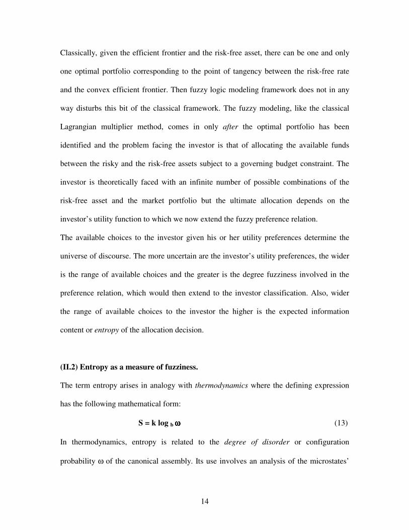
(II.2) Entropy as a measure of fuzziness.

The term entropy arises in analogy with thermodynamics where the defining expression

has the following mathematical form:

S = k log b ωωωω (13)

In thermodynamics, entropy is related to the degree of disorder or configuration

probability ω of the canonical assembly. Its use involves an analysis of the microstates’

15

distribution in the canonical assembly among the available energy levels for both

isothermal reversible and isothermal irreversible (spontaneous) processes (with an

attending modification). The physical scale factor k is the Boltzmann constant. [7]

However, the thermodynamic form has a different sign and the word negentropy is

therefore sometimes used to denote expected information. Though Claude Shannon

originally conceptualized the entropy measure of expected information, it was DeLuca

and Termini who brought this concept in the realms of fuzzy mathematics when they

sought to derive a universal mathematical measure of fuzziness.

Let us consider the fuzzy subset F = {r1/X, r2/Y}, 0 ≤ (r1, r2) ≤ 1, where X is the event

(y<x) and Y is the event (y≥x), x being the proportion of funds to be invested in the

market portfolio and y being the proportion of funds to be invested in the risk-less

security. Then the DeLuca-Termini conditions for measure of fuzziness may be stated as

follows: [3]

• FUZ (F) = 0 if F is a crisp set i.e. if the investor classified under a particular risk

category always invests entire funds either in the risk-free asset (conservative

attitude) or in the market portfolio (aggressive attitude)

• FUZ (F) = Max FUZ (F) when F = (0.5/X, 0.5/Y)

• FUZ (F) ≥≥≥≥ FUZ (F*) if F* is a sharpened version of F, i.e. if F* is a fuzzy subset

satisfying F*(ri) ≥ F (ri) given that F (ri) ≥ 0.5 and F (ri) ≥ F*(ri) given that 0.5 ≥ F (ri)

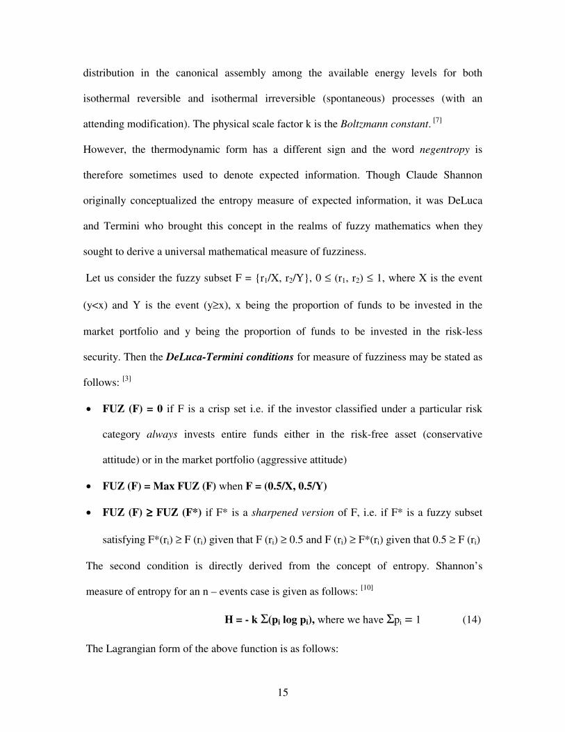
The second condition is directly derived from the concept of entropy. Shannon’s

measure of entropy for an n – events case is given as follows: [10]

H = - k Σ(pi log pi), where we have Σpi = 1 (14)

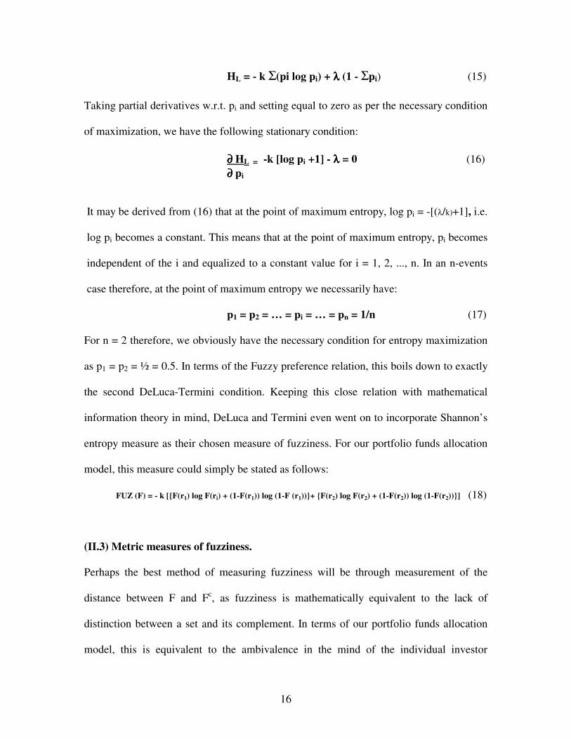
The Lagrangian form of the above function is as follows:

16

HL = - k Σ(pi log pi) + λλλλ (1 - Σpi) (15)

Taking partial derivatives w.r.t. pi and setting equal to zero as per the necessary condition

of maximization, we have the following stationary condition:

∂∂∂∂ HL = -k [log pi +1] - λλλλ = 0 (16) ∂∂∂∂ pi

It may be derived from (16) that at the point of maximum entropy, log pi = -[(λ/k)+1], i.e.

log pi becomes a constant. This means that at the point of maximum entropy, pi becomes

independent of the i and equalized to a constant value for i = 1, 2, ..., n. In an n-events

case therefore, at the point of maximum entropy we necessarily have:

p1 = p2 = … = pi = … = pn = 1/n (17)

For n = 2 therefore, we obviously have the necessary condition for entropy maximization

as p1 = p2 = ½ = 0.5. In terms of the Fuzzy preference relation, this boils down to exactly

the second DeLuca-Termini condition. Keeping this close relation with mathematical

information theory in mind, DeLuca and Termini even went on to incorporate Shannon’s

entropy measure as their chosen measure of fuzziness. For our portfolio funds allocation

model, this measure could simply be stated as follows:

FUZ (F) = - k [{F(r1) log F(ri) + (1-F(r1)) log (1-F (r1))}+ {F(r2) log F(r2) + (1-F(r2)) log (1-F(r2))}] (18)

(II.3) Metric measures of fuzziness.

Perhaps the best method of measuring fuzziness will be through measurement of the

distance between F and Fc, as fuzziness is mathematically equivalent to the lack of

distinction between a set and its complement. In terms of our portfolio funds allocation

model, this is equivalent to the ambivalence in the mind of the individual investor

17

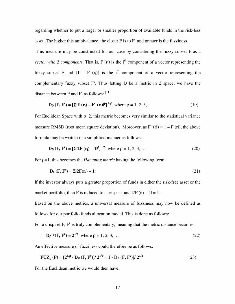
regarding whether to put a larger or smaller proportion of available funds in the risk-less

asset. The higher this ambivalence, the closer F is to Fc and greater is the fuzziness.

This measure may be constructed for our case by considering the fuzzy subset F as a

vector with 2 components. That is, F (ri) is the ith component of a vector representing the

fuzzy subset F and (1 – F (ri)) is the ith component of a vector representing the

complementary fuzzy subset Fc. Thus letting D be a metric in 2 space; we have the

distance between F and Fc as follows: [11]

Dρρρρ (F, Fc) = [ΣΣΣΣ|F (ri) – Fc (ri)|ρρρρ] 1/ρρρρ, where ρ = 1, 2, 3, … (19)

For Euclidean Space with ρ=2, this metric becomes very similar to the statistical variance

measure RMSD (root mean square deviation). Moreover, as Fc (ri) = 1 – F (ri), the above

formula may be written in a simplified manner as follows:

Dρρρρ (F, Fc) = [ΣΣΣΣ|2F (ri) – 1|ρρρρ] 1/ρρρρ, where ρ = 1, 2, 3, … (20)

For ρ=1, this becomes the Hamming metric having the following form:

D1 (F, Fc) = ΣΣΣΣ|2F(ri) – 1| (21)

If the investor always puts a greater proportion of funds in either the risk-free asset or the

market portfolio, then F is reduced to a crisp set and |2F (ri) – 1| = 1.

Based on the above metrics, a universal measure of fuzziness may now be defined as

follows for our portfolio funds allocation model. This is done as follows:

For a crisp set F, Fc is truly complementary, meaning that the metric distance becomes:

Dρρρρ *(F, Fc) = 21/ρρρρ, where ρ = 1, 2, 3, … (22)

An effective measure of fuzziness could therefore be as follows:

FUZρρρρ (F) = [21/ρρρρ - Dρρρρ (F, Fc)]/ 21/ρρρρ = 1 - Dρρρρ (F, Fc)]/ 21/ρρρρ (23)

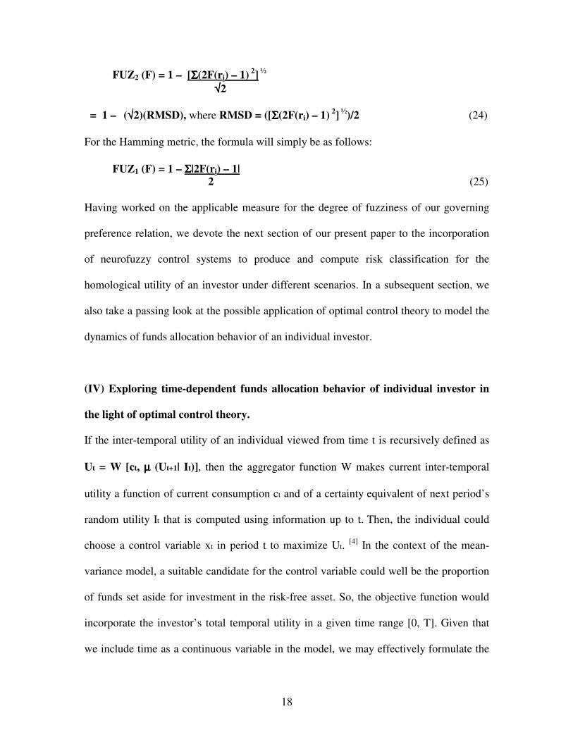
For the Euclidean metric we would then have:

18

FUZ2 (F) = 1 – [ΣΣΣΣ(2F(ri) – 1) 2] ½

√√√√2 = 1 – (√√√√2)(RMSD), where RMSD = ([ΣΣΣΣ(2F(ri) – 1) 2] ½)/2 (24)

For the Hamming metric, the formula will simply be as follows:

FUZ1 (F) = 1 – ΣΣΣΣ|2F(ri) – 1| 2 (25)

Having worked on the applicable measure for the degree of fuzziness of our governing

preference relation, we devote the next section of our present paper to the incorporation

of neurofuzzy control systems to produce and compute risk classification for the

homological utility of an investor under different scenarios. In a subsequent section, we

also take a passing look at the possible application of optimal control theory to model the

dynamics of funds allocation behavior of an individual investor.

(IV) Exploring time-dependent funds allocation behavior of individual investor in

the light of optimal control theory.

If the inter-temporal utility of an individual viewed from time t is recursively defined as

Ut = W [ct, µµµµ (Ut+1| It)], then the aggregator function W makes current inter-temporal

utility a function of current consumption ct and of a certainty equivalent of next period’s

random utility It that is computed using information up to t. Then, the individual could

choose a control variable xt in period t to maximize Ut. [4] In the context of the mean-

variance model, a suitable candidate for the control variable could well be the proportion

of funds set aside for investment in the risk-free asset. So, the objective function would

incorporate the investor’s total temporal utility in a given time range [0, T]. Given that

we include time as a continuous variable in the model, we may effectively formulate the

19

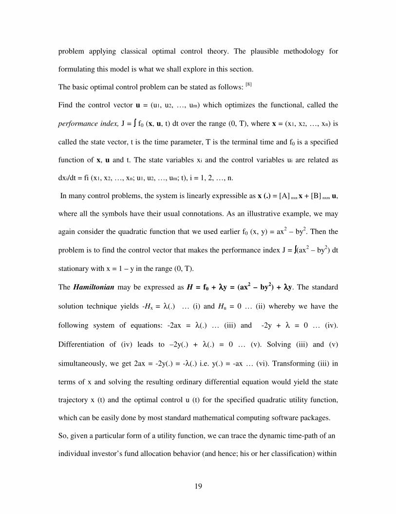
problem applying classical optimal control theory. The plausible methodology for

formulating this model is what we shall explore in this section.

The basic optimal control problem can be stated as follows: [8]

Find the control vector u = (u1, u2, …, um) which optimizes the functional, called the

performance index, J = ∫∫∫∫ f0 (x, u, t) dt over the range (0, T), where x = (x1, x2, …, xn) is

called the state vector, t is the time parameter, T is the terminal time and f0 is a specified

function of x, u and t. The state variables xi and the control variables ui are related as

dxi/dt = fi (x1, x2, …, xn; u1, u2, …, um; t), i = 1, 2, …, n.

In many control problems, the system is linearly expressible as x (.) = [A] nxn x + [B] nxm u,

where all the symbols have their usual connotations. As an illustrative example, we may

again consider the quadratic function that we used earlier f0 (x, y) = ax2 – by2. Then the

problem is to find the control vector that makes the performance index J = ∫∫∫∫(ax2 – by2) dt

stationary with x = 1 – y in the range (0, T).

The Hamiltonian may be expressed as H = f0 + λλλλy = (ax2 – by2) + λλλλy. The standard

solution technique yields -Hx = λ(.) … (i) and Hu = 0 … (ii) whereby we have the

following system of equations: -2ax = λ(.) … (iii) and -2y + λ = 0 … (iv).

Differentiation of (iv) leads to –2y(.) + λ(.) = 0 … (v). Solving (iii) and (v)

simultaneously, we get 2ax = -2y(.) = -λ(.) i.e. y(.) = -ax … (vi). Transforming (iii) in

terms of x and solving the resulting ordinary differential equation would yield the state

trajectory x (t) and the optimal control u (t) for the specified quadratic utility function,

which can be easily done by most standard mathematical computing software packages.

So, given a particular form of a utility function, we can trace the dynamic time-path of an

individual investor’s fund allocation behavior (and hence; his or her classification) within

20

the ambit of the mean-variance model by obtaining the state trajectory of x – the

proportion of funds invested in the market portfolio and the corresponding control

variable y – the proportion of funds invested in the risk-free asset using the standard

techniques of optimal control theory.

References:

Book, Journals, and Working Papers:

[1] Arkes, Hal R., Connolly, Terry, and Hammond, Kenneth R., “Judgment And Decision Making – An Interdisciplinary Reader” Cambridge Series on Judgment and Decision Making, Cambridge University Press, 2nd Ed., 2000, 233-39 [2] Chiang, Alpha C., “Fundamental Methods of Mathematical Economics” McGraw-Hill International Editions, Economics Series, 3rd Ed. 1984, 401-408 [3] DeLuca A.; and Termini, S., “A definition of a non-probabilistic entropy in the setting of fuzzy sets”, Information and Control 20, 1972, 301-12 [4] Haliassos, Michael and Hassapis, Christis, “Non-Expected Utility, Savings and Portfolios” The Economic Journal, Royal Economic Society, January 2001, 69-73 [5] Kolb, Robert W., “Investments” Kolb Publishing Co., U.S.A., 4th Ed. 1995, 253-59 [6] Korsan, Robert J., “Nothing Ventured, Nothing Gained: Modeling Venture Capital Decisions” Decisions, Uncertainty and All That, The Mathematica Journal, Miller Freeman Publications 1994, 74-80 [7] Oxford Science Publications, Dictionary of Computing OUP, N.Y. USA, 1984 [8] S.S. Rao, Optimization theory and applications, New Age International (P) Ltd., New Delhi, 2nd Ed., 1995, 676-80 [9] Sarin, Rakesh K. & Peter Wakker, “Benthamite Utility for Decision Making” Submitted Report, Medical Decision Making Unit, Leiden University Medical Center, The Netherlands, 1997, 3-20 [10] Swarup, Kanti, Gupta, P. K.; and Mohan, M., Tracts in Operations Research Sultan Chand & Sons, New Delhi, 8th Ed., 1997, 659-92

21

[11] Yager, Ronald R.; and Filev, Dimitar P., Essentials of Fuzzy Modeling and Control John Wiley & Sons, Inc. USA 1994, 7-22 [12] Zadrozny, Slawmir “An Approach to the Consensus Reaching Support in Fuzzy Environment”, Consensus Under Fuzziness edited by Kacprzyk, Januz, Hannu, Nurmi and Fedrizzi, Mario, International Series in Intelligent Systems, USA, 1997, 87-90 Website References: 1 http://www.fuzzytech.com/e/e_ft4bf6.html

2 http://www.geocities.com/wallstreet/bureau/3486/11.htm