Futuristic Projection of Solid Waste Generation in ...283-299)V10N13CT.pdf · Futuristic Projection of Solid Waste Generation in Dehradun City of Uttarakhand using Supervised Artificial

Futuristic Projection of Solid Waste Generation in Dehradun City of Uttarakhand using Supervised Artificial Neural Network-Non-Linear Autoregressive Neural Network

(NARnet)

Ritesh Saini1*, Neelu J. Ahuja2, Kanchan Deoli Bahukhandi3

1College of Engineering Studies, University of Petroleum & Energy Studies, Dehradun, Phone no:+91-7409847176

2Department of Centre for Information Technology, University of Petroleum & Energy Studies, Dehradun, Phone no:+91-9411384390

3Department of Health, Safety & Environment Engineering, University of Petroleum & Energy Studies, Dehradun .

Abstract : Solid waste management has become a pressing problem in every city. Municipal

Solid Waste characteristics and quantities change significantly with time. The model in the

present study enables the solid waste management personnel to have prior information on the

amount of future waste. A prediction model has been developed that uses the present waste

generation data, along with different environmental and economic factors. These factors have been implicitly incorporated using quantity of solid waste as a time-series dataset to simulate a

supervised Artificial Neural Network (ANN) in MATLAB - Nonlinear Autoregressive Neural

Network (NARnet). The values of input parameter current solid waste quantity are used for estimation of output which is, amount of solid waste generated for future period of about three

months, thus facilitating the pre-planning of waste management. In current work different

architectures of neural network have been examined by varying the combinations of number of hidden layers, neurons in each layer and the choice of activation functions. Based on the

performance criteria, the best optimized ANN architecture has been used for the prediction of

quantity of solid waste.

Keywords : solid waste generation, artificial neural network, time series data, prediction of solid waste quantity.

1. Introduction

Municipal solid waste characteristics and quantities change significantly with time. Some of the

affecting factors include - change in the food consumption pattern, population growth, migration, underlying economic development, employment changes, weather conditions, geographical situation, hobbies, and

household size1. All these factors along with response to recycling of waste influence the future generation of

solid waste tremendously. This warrants a need to design and develop a reliable model to assess the impact of factors, affecting solid waste generation. The model is proposed to provide prediction that will play a very

important role in overall process of management and disposal of the solid waste that may be generated in future.

The model enables the solid waste management personnel to have prior information on the amount of future waste. Thus, facilitating its disposal planning.

International Journal of ChemTech Research CODEN (USA): IJCRGG, ISSN: 0974-4290, ISSN(Online):2455-9555

Vol.10 No.13, pp 283-299, 2017

Ritesh Saini et al /International Journal of ChemTech Research, 2017,10(13): 283-299. 284

Prime prerequisite for Solid Waste Management system is reasonably reliable solid waste quantity

prediction. The available statistical models work very well with data which are linear in nature and can fit into

one of the existing trends. But the solid waste data representing quantity of waste collected by local SWM authorities -on-day- to day basis are nonlinear (wt. in metric tonnes) in nature, due to which, the prediction with

accuracy by the use of statistical models becomes a challenge. Prediction of solid waste generation though use

of ANN is widely available in literature. Determination of solid waste quantity generated in future is a useful

scientific advance from planning perspective and would provide the time and opportunity for the solid waste personnel and their organization to adopt necessary steps required for the disposal such as capacity, machinery

and estimated area for a municipal landfill expected to be used in future. If this information is known well in

advance to the concerned authorities, the complete process of solid waste disposal from collection to its choice of disposal methods can be planned well in advance and be much more organized. This would result in a more

effective solid waste management system for the city.

Located in the lush green Garhwal region, 236 km to the north of Indian sub-continent is a valley called

Dehradun. It is the capital of the state of Uttarakhand. The population of the city is about 578,420(2011 census).

Dehradun is in the foothills of Himalayas nestled between the Ganga on the east and the Yamuna on the west.

The city is well connected and in proximity to Mussoorie and Auli, popular himalayan tourist destinations, Haridwar, Rishikesh holy cities and the himalayan pilgrimage circuit of Char Dham.

This makes Dehradun city a tourist hot spot causing migration patterns that are seasonal in nature. Being the current capital of Uttarakhand, the growth rate of the city is on the rise. Coupled with this is the

industrialization in the vicinity, generating multitude of job opportunities for people in and around the city

resulting in migration of workforce. In recent years, the increase in emigration has created an increase in waste generation resulting in municipal solid waste menace. Though the idealistic approach of waste management is

to control waste generation at source, aiming towards a zero waste, as per the current scenario, the city of

Dehradun is far from it. This necessitates the focus towards waste handling, which is very likely to be improved

provided, necessary planning is invested upon. An appropriate model for the prediction of future values of solid waste is essential for the proper plan and choice of waste disposal methods in future.

2. Related Work

McBean and Fortin worked with municipal solid waste management using socio-economic factors, their

correlations, solid waste composition and quantities. Their model uses generation coefficients associated with individual material components for estimation of the quantity of solid waste generated by the domestic and

industrial sources2. Dyson and Chang considered the factors such as effects of population, level of income, and

the size of dwelling unit in a linear regression model which was unable to handle various issues. A new approach, namely system dynamics modeling- presents various trends of solid waste generation in a rapidly

growing urban area with a limited base of samples using simulation tool-Stella3. Beigl et al.used a model for the

European cities, that made use of the explanatory variables, Gross Domestic Product rate of infant mortality

rate, such as size of household, which were termed as one of the core set of significant regional development indicators. Evaluation of the data collected by them indicated a significant relation between regional

development and municipal solid waste generation4. Benitez et al. gave prediction for the residential solid waste

by development of a linear mathematical model using education, income per household, and number of members in family, being used as explanatory variables

5. Buenrostro et al. reported income as an influential

factor for solid waste generation by forecasting both the residential and the non-residential solid waste using

multiple linear regression analysis6. Dayal et al. investigated and assessed climatic conditions and socio-

economic status, as holding heavy impact on solid waste characteristics7.

Recently, there have been some investigations to assess the application of the artificial neural networks

(ANN)-multi-layer perceptron-in short-term and medium-term forecasting, but very limited efforts have been condu Futuristic Projection of Solid Waste Generation in Dehradun City of Uttarakhand using

Supervised Artificial Neural Network-Non-Linear Autoregressive Neural Network (NARnet) cted for the

long-term forecasting. Kumar et al. have used radial basis function approach of artificial neural network model for the long term forecast of solid waste for the city of Eluru and to reduce the discrepancy between the

predicted value and the observed value of the municipal solid waste8. Zade and Noori predicted weekly solid

waste values, using feed forward ANN by taking the generated waste as a time series input to the neural

network for the city of Mashhad, emphasizing ANN as prediction tool9. Noori et al. extended the previous study


with the application of Principal Component Analysis and Gamma test techniques for weekly forecasting. They

applied these techniques on the set of influential input parameters to find those which affect the generation of

solid waste the most. In their study they have also compared a few ANN training algorithms. Their results show that with different pre-processing technique a different algorithm would provide the best result. They concluded

that both the pre-processing techniques were almost similar hence, either can be used10

.

Noori et al. evaluated results of the uncertainty of predictions of solid waste generation by hybrid of

wavelet transform-ANN and wavelet transform-ANFIS models11

. Noori et al. gave an improved Support Vector

Machine model, using combination of both the PCA and SVM techniques for prediction of weekly generation

of solid waste of Mashhad city. This model has more advantages over the traditional SVM model as noted by the author

12. Karaca and Ozkaya were able to control the leachate generation rate in landfills by the use of

ANN. They selected the best network architecture, training algorithm and have also discussed further

development along with the advantages and the disadvantages13

. Using a limited sample set Chen and Chang reported a new theory gray fuzzy dynamic modeling, for solid waste prediction in urban areas

14.

In multivariate models, solid waste generation can be presented as a delay of time. The time delay would easily represent the dependency of an input parameter on itself for a particular period of time. Due to

high correlation observed between dependent variable and same variable intervals, the delaying of the

parameters has significant impact on prediction of generation of solid waste. This serves in the model as an

independent variable1. As the input parameter depends on itself, the effect of the other parameters for the past

few measures becomes indirectly included for the current value. For this reason, the effects of the other input

parameters aiding in the prediction of future generation of solid waste are negligible. Due to this there is no

need to model other factors that may have effect on the generation of solid waste.

3. Materials& Methods

3.1. Current Work

The purpose of current work is to provide a reasonably accurate and reliable model for the prediction of

solid waste with an aim to decrease the uncertainty present in prediction. The purpose is also to predict the future measures of weekly solid waste generated (possibly a period of 12 weeks). This futuristic prediction is

proposed to be a useful advance in the proper planning and organization of the solid waste and its disposal.

In the current work, those variables which have the highest influence on SWG are selected as the input

parameters. The choice of the selected variables depends on the attributes, such as their ability to be forecasted

for a long forecasting horizon and the relative high accuracy with which the forecast can be made. Few such

factors identified with the highest impact on solid waste prediction are population and household size. After the selection of parameters, the developed ANN model is trained, tested and validated for the period for which data

have been collected, and the model architecture found most reliable is determined based on the selected

performance measures. Eventually, the predicted future values based on the currently available data are validated.

3.2. Preprocessing

Before modeling the neural network, it is essential to refine the data by pre-processing techniques due

to the following reasons: noise reduction and low learning rates of ANN. The various parameters for generation of solid waste are taken as, population growth, economic development and household size

1. The parameter solid

waste can be presented as a delay of time and incorporated as an independent variable in the model and hence,

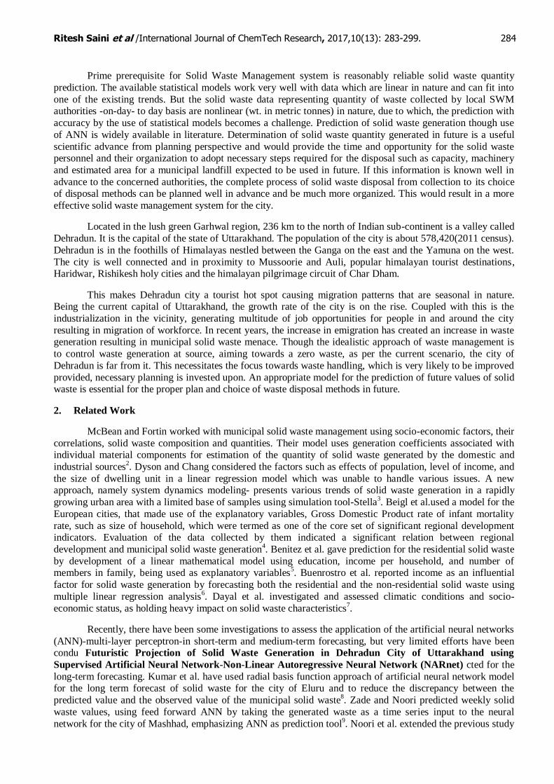
in the present work, the input parameter is only solid waste generated1. The weekly time series data set of the

input parameter is depicted in Figure 1.


Figure 1. Collected Data

After the training of the network is completed, this ANN model is used for future value prediction. The

results of training the ANN on the raw collected data would make it evident that the independent variable in future prediction would be highly changed with respect to the data from the observed period.

To make the model being trained in range of the observed data meet the values occuring in the predicted range, the observed data needs to be taken to the same scale as data from the prediction period i.e.

pre-processing of data. To achieve this goal, the Stationary Chain concept in time series is used. A time series

variable is said to be stationary when statistical measures such as mean, variance, and correlation coefficients remain constant over a period of time.

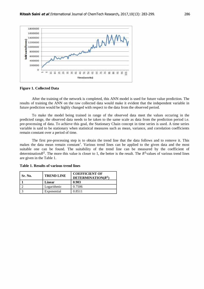
The first pre-processing step is to obtain the trend line that the data follows and to remove it. This makes the data mean remain constant

1. Various trend lines can be applied to the given data and the most

suitable one can be found. The suitability of the trend line can be measured by the coefficient of

determination . The more this value is closer to 1, the better is the result. The values of various trend lines

are given in the Table 1.

Table 1. Results of various trend lines

Sr. No. TREND LINE COEFFICIENT OF

DETERMINATION( )

1 Linear 0.903

2 Logarithmic 0.7506

3 Exponential 0.8511


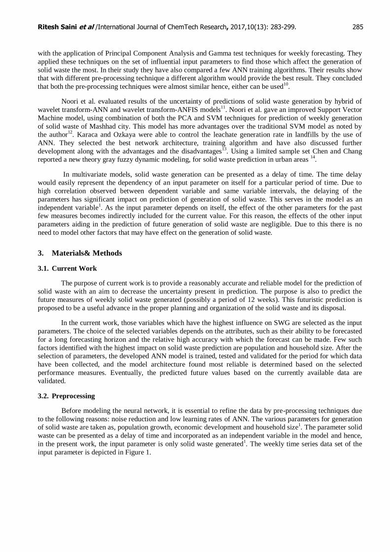
Figure 2. Trend of generated solid waste for the observed period

From Table 1 it can be observed that the data follows the linear trend line, the Figure 2 depicts this

trend line onto the data. The equation for the linear trend line is given by Equation 1.

(1)

where y is the solid waste amount and x is the week number for which it is being calculated.

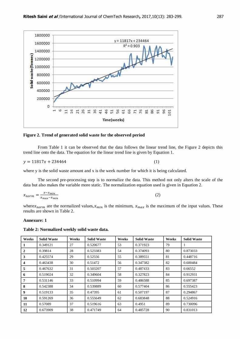
The second pre-processing step is to normalize the data. This method not only alters the scale of the

data but also makes the variable more static. The normalization equation used is given in Equation 2.

(2)

where are the normalized values, is the minimum, is the maximum of the input values. These

results are shown in Table 2.

Annexure: 1

Table 2: Normalized weekly solid waste data.

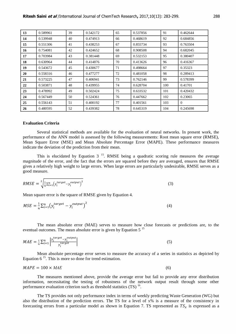
Weeks Solid Waste Weeks Solid Waste Weeks Solid Waste Weeks Solid Waste

1 0.349121 27 0.520677 53 0.371923 79 1

2 0.39814 28 0.523383 54 0.374093 80 0.873033

3 0.425574 29 0.52556 55 0.389551 81 0.448716

4 0.463438 30 0.51472 56 0.347382 82 0.600484

5 0.467632 31 0.503207 57 0.487433 83 0.66552

6 0.519024 32 0.349604 58 0.327823 84 0.912931

7 0.531146 33 0.510994 59 0.486588 85 0.697387

8 0.542388 34 0.539889 60 0.577404 86 0.555423

9 0.519133 35 0.47395 61 0.507197 87 0.294867

10 0.591269 36 0.555649 62 0.683848 88 0.524916

11 0.57089 37 0.519616 63 0.4951 89 0.730096

12 0.673909 38 0.471749 64 0.485728 90 0.831013


13 0.589961 39 0.542172 65 0.537856 91 0.462644

14 0.539948 40 0.474913 66 0.468619 92 0.684856

15 0.551306 41 0.438253 67 0.855734 93 0.763504

16 0.754081 42 0.424652 68 0.908508 94 0.682045

17 0.703984 43 0.381448 69 0.532153 95 0.380407

18 0.630964 44 0.414876 70 0.413626 96 0.416367

19 0.543672 45 0.430677 71 0.498664 97 0.35323

20 0.558316 46 0.477277 72 0.481058 98 0.289413

21 0.573225 47 0.406941 73 0.762146 99 0.578399

22 0.503871 48 0.439955 74 0.628704 100 0.41701

23 0.478992 49 0.502424 75 0.633532 101 0.420432

24 0.567449 50 0.524361 76 0.447662 102 0.23065

25 0.556143 51 0.400192 77 0.401561 103 0

26 0.480595 52 0.439382 78 0.645319 104 0.245698

Evaluation Criteria

Several statistical methods are available for the evaluation of neural networks. In present work, the performance of the ANN model is assessed by the following measurements: Root mean square error (RMSE),

Mean Square Error (MSE) and Mean Absolute Percentage Error (MAPE). These performance measures

indicate the deviation of the prediction from their mean.

This is elucidated by Equation 3 15

. RMSE being a quadratic scoring rule measures the average

magnitude of the error, and the fact that the errors are squared before they are averaged, ensures that RMSE

gives a relatively high weight to large errors. When large errors are particularly undesirable, RMSE serves as a good measure.

√

∑ (

)

(3)

Mean square error is the square of RMSE given by Equation 4.

∑ (

)

(4)

The mean absolute error (MAE) serves to measure how close forecasts or predictions are, to the eventual outcomes. The mean absolute error is given by Equation 5

15

∑ |

|

(5)

Mean absolute percentage error serves to measure the accuracy of a series in statistics as depicted by

Equation 6 15

. This is more so done for trend estimation.

(6)

The measures mentioned above, provide the average error but fail to provide any error distribution information, necessitating the testing of robustness of the network output result through some other

performance evaluation criterion such as threshold statistics (TS) 16

.

The TS provides not only performance index in terms of weekly predicting Waste Generation (WG) but

also the distribution of the prediction errors. The TS for a level of x% is a measure of the consistency in

forecasting errors from a particular model as shown in Equation 7. TS represented as is expressed as a


percentage. This criterion can be represented for various levels of absolute error (AE) from the model. For x%

level it is computed as given in Equation 7.

( ) (7)

where is the number of predicted WG (out of n total computed) for which AE is less than x% from the model.

4. Artificial Neural Network

Recent literature shows, artificial neural network (ANN) has been used in nonlinear system modeling

where functional relationship between input and output variables is not known. ANNs designed and developed

as cellular information processors work on the perceived notion of the human brain and its neural system. One of the significant factors of ANNs is its ability to learn. After the process of learning, it can construct a complex

nonlinear system through a set of input/output samples. Therefore, ANN is amply trusted for modeling the solid

waste generation and make futuristic predictions.

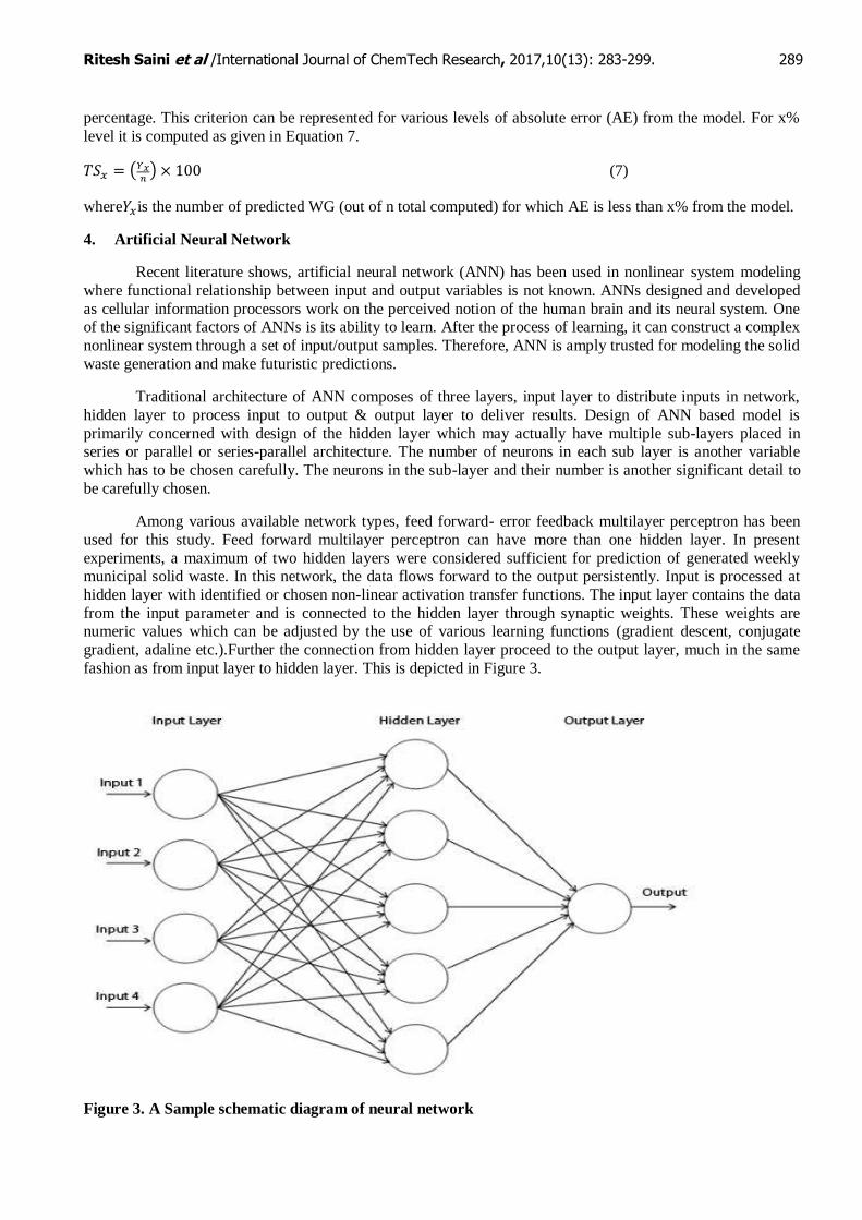
Traditional architecture of ANN composes of three layers, input layer to distribute inputs in network,

hidden layer to process input to output & output layer to deliver results. Design of ANN based model is

primarily concerned with design of the hidden layer which may actually have multiple sub-layers placed in series or parallel or series-parallel architecture. The number of neurons in each sub layer is another variable

which has to be chosen carefully. The neurons in the sub-layer and their number is another significant detail to

be carefully chosen.

Among various available network types, feed forward- error feedback multilayer perceptron has been

used for this study. Feed forward multilayer perceptron can have more than one hidden layer. In present

experiments, a maximum of two hidden layers were considered sufficient for prediction of generated weekly municipal solid waste. In this network, the data flows forward to the output persistently. Input is processed at

hidden layer with identified or chosen non-linear activation transfer functions. The input layer contains the data

from the input parameter and is connected to the hidden layer through synaptic weights. These weights are numeric values which can be adjusted by the use of various learning functions (gradient descent, conjugate

gradient, adaline etc.).Further the connection from hidden layer proceed to the output layer, much in the same

fashion as from input layer to hidden layer. This is depicted in Figure 3.

Figure 3. A Sample schematic diagram of neural network


The output obtained at each neuron is a function of its inputs. The output of the jth neuron in any layer

is shown below by Equations 8 and 9.

∑ (8)

( ) (9)

Except in input layer, for every neuron, j, in a layer, each of the i inputs, , to that layer is multiplied

by a previously established weight, . These are summed together and resulting value, , is then biased by a

previously established threshold value, , and sent through an activation function (usually sigmoid function), f.

The resulting output, , acts as an input to the next layer or is the final output, assuming there are no more

hidden layers.

One of the learning rule for multilayer perceptron is the error back propagation. In present work, the delaying variables that decrease the accuracy of forecasting have not been used, because they increase the error

in long-term forecasting significantly. Default network type for most MLPs is feed forward back propagated

multi-layer perception. The architecture with multiple neuron layers with non-linear transfer functions, permits

learning of non-linear and linear relationships between input and output vectors by the network.

Some of the training algorithms that can be used are: gradient descent, conjugate gradient and

levenberg-marquardt. The standard back propagation algorithm adjusts the weights in the steepest descent direction (negative of the gradient), which the performance function is decreasing most rapidly. In the CG

algorithms, a search is performed along conjugate directions for faster convergence than steepest descent

directions. Levenberg -Marquardt algorithm is designed to approach second order training speed without having to compute the Hessian matrix.

The use of STA (Stop Training Algorithm) reduced the training time four times and it provided better

and more reliable generalization performance. The available data are split into three parts: (1) Training Set (2) Testing Set (3) Validation Set. To determine the network parameters weights and biases, the training set data is

used. To assess the strength and utility of the predicted relationship and to verify the effectiveness of the

stopping criterion, the testing set data is used. To avoid over fitting and to estimate the network performance and decide when the training stopped, the validation set data is used. This division of data implements STA in

practice.

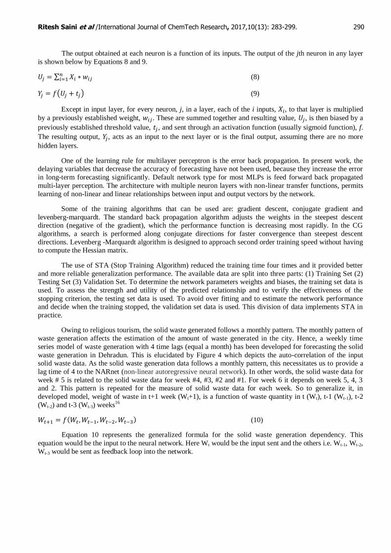
Owing to religious tourism, the solid waste generated follows a monthly pattern. The monthly pattern of

waste generation affects the estimation of the amount of waste generated in the city. Hence, a weekly time

series model of waste generation with 4 time lags (equal a month) has been developed for forecasting the solid

waste generation in Dehradun. This is elucidated by Figure 4 which depicts the auto-correlation of the input solid waste data. As the solid waste generation data follows a monthly pattern, this necessitates us to provide a

lag time of 4 to the NARnet (non-linear autoregressive neural network). In other words, the solid waste data for

week # 5 is related to the solid waste data for week #4, #3, #2 and #1. For week 6 it depends on week 5, 4, 3 and 2. This pattern is repeated for the measure of solid waste data for each week. So to generalize it, in

developed model, weight of waste in t+1 week (Wt+1), is a function of waste quantity in t (Wt), t-1 (Wt-1), t-2

(Wt-2) and t-3 (Wt-3) weeks16

( ) (10)

Equation 10 represents the generalized formula for the solid waste generation dependency. This

equation would be the input to the neural network. Here Wt would be the input sent and the others i.e. Wt-1, Wt-2,

Wt-3 would be sent as feedback loop into the network.


Figure 4. Auto-Correlation of input data

4.1. The ANN Model

Data analysis and pre-processing are very important steps before utilizing the data. After pre-

processing, the artificial neural network model was developed based on the nonlinear autoregressive network (NARnet). In this network the output of the network goes as a feedback to the input layer. In present work, a

number of design factors were considered for the modeling of the neural network like the number of neurons in

hidden layers. Different activation functions were tested. After careful investigation in each layer: a sigmoidal function for the hidden layer and a linear function for the output layer were selected. The hidden layers were

varied between 1-2 layers as a maximum of two hidden layer results in best outputs without making the network

too complicated and different numbers of neurons (5-20) were applied to the hidden layers.

After pre-processing, input data was classified to three blocks; 70% for training, 15% for validation,

and 15% for testing. Owing to validation error increased six times sequentially, the training would stop.

Training was restarted using network weights, obtained from previous run until acceptable results were reached.

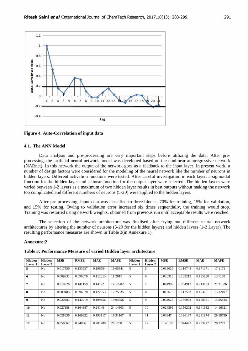
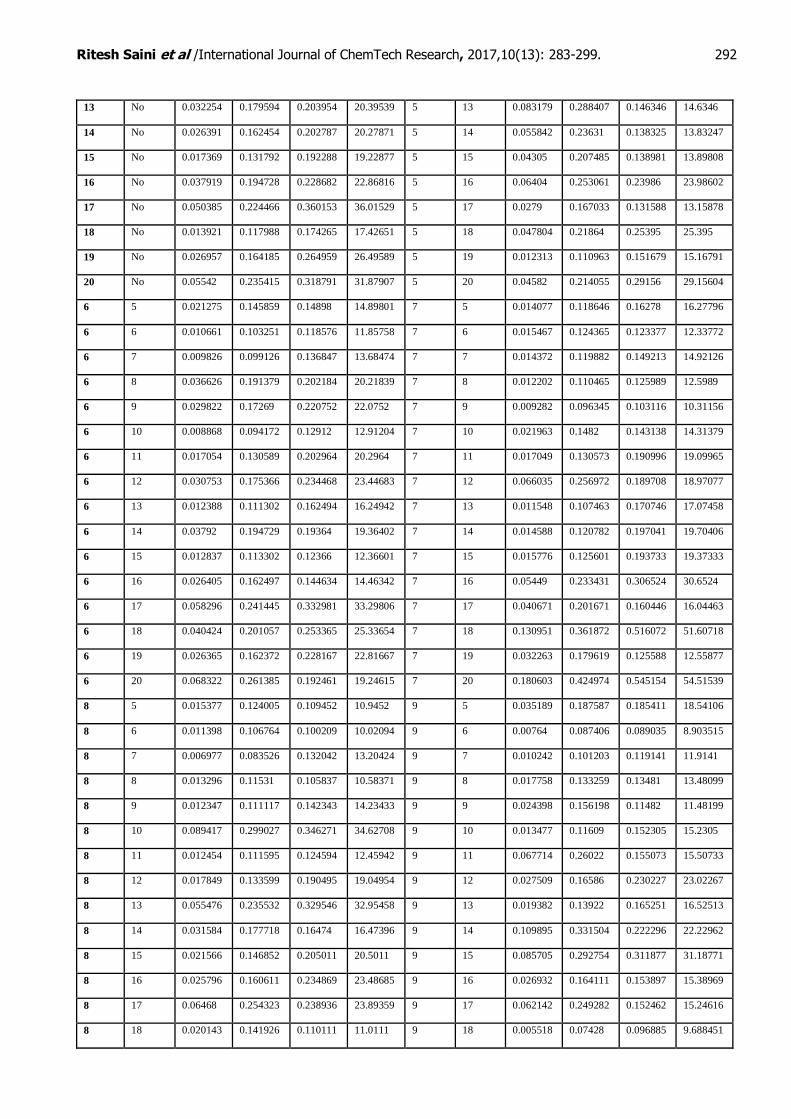
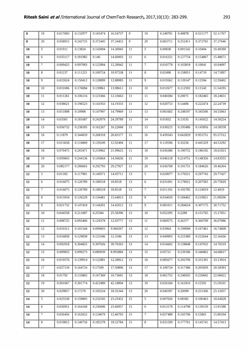
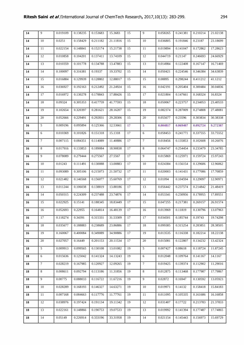
The selection of the network architecture was finalised after trying out different neural network

architectures by altering the number of neurons (5-20 for the hidden layers) and hidden layers (1-2 Layer). The resulting performance measures are shown in Table 3(in Annexure 1).

Annexure:2

Table 3: Performance Measure of varied Hidden layer architecture

Hidden

Layer 1

Hidden

Layer 2

MSE RMSE MAE MAPE Hidden

Layer 1

Hidden

Layer 2

MSE RMSE MAE MAPE

5 No 0.017859 0.133637 0.196584 19.65841 5 5 0.013629 0.116744 0.171171 17.1171

6 No 0.009231 0.096079 0.112815 11.2815 5 6 0.026313 0.162213 0.135188 13.5188

7 No 0.019926 0.141159 0.14122 14.12202 5 7 0.041989 0.204912 0.213133 21.31326

8 No 0.009405 0.096978 0.122553 12.25535 5 8 0.012675 0.112583 0.15325 15.32497

9 No 0.020283 0.142419 0.199456 19.94556 5 9 0.034625 0.186078 0.158581 15.85815

10 No 0.027188 0.164887 0.24148 24.14803 5 10 0.024399 0.156202 0.141632 14.16321

11 No 0.028636 0.169222 0.193117 19.31167 5 11 0.03847 0.196137 0.291874 29.18739

12 No 0.058062 0.24096 0.201288 20.1288 5 12 0.140193 0.374423 0.283277 28.3277


13 No 0.032254 0.179594 0.203954 20.39539 5 13 0.083179 0.288407 0.146346 14.6346

14 No 0.026391 0.162454 0.202787 20.27871 5 14 0.055842 0.23631 0.138325 13.83247

15 No 0.017369 0.131792 0.192288 19.22877 5 15 0.04305 0.207485 0.138981 13.89808

16 No 0.037919 0.194728 0.228682 22.86816 5 16 0.06404 0.253061 0.23986 23.98602

17 No 0.050385 0.224466 0.360153 36.01529 5 17 0.0279 0.167033 0.131588 13.15878

18 No 0.013921 0.117988 0.174265 17.42651 5 18 0.047804 0.21864 0.25395 25.395

19 No 0.026957 0.164185 0.264959 26.49589 5 19 0.012313 0.110963 0.151679 15.16791

20 No 0.05542 0.235415 0.318791 31.87907 5 20 0.04582 0.214055 0.29156 29.15604

6 5 0.021275 0.145859 0.14898 14.89801 7 5 0.014077 0.118646 0.16278 16.27796

6 6 0.010661 0.103251 0.118576 11.85758 7 6 0.015467 0.124365 0.123377 12.33772

6 7 0.009826 0.099126 0.136847 13.68474 7 7 0.014372 0.119882 0.149213 14.92126

6 8 0.036626 0.191379 0.202184 20.21839 7 8 0.012202 0.110465 0.125989 12.5989

6 9 0.029822 0.17269 0.220752 22.0752 7 9 0.009282 0.096345 0.103116 10.31156

6 10 0.008868 0.094172 0.12912 12.91204 7 10 0.021963 0.1482 0.143138 14.31379

6 11 0.017054 0.130589 0.202964 20.2964 7 11 0.017049 0.130573 0.190996 19.09965

6 12 0.030753 0.175366 0.234468 23.44683 7 12 0.066035 0.256972 0.189708 18.97077

6 13 0.012388 0.111302 0.162494 16.24942 7 13 0.011548 0.107463 0.170746 17.07458

6 14 0.03792 0.194729 0.19364 19.36402 7 14 0.014588 0.120782 0.197041 19.70406

6 15 0.012837 0.113302 0.12366 12.36601 7 15 0.015776 0.125601 0.193733 19.37333

6 16 0.026405 0.162497 0.144634 14.46342 7 16 0.05449 0.233431 0.306524 30.6524

6 17 0.058296 0.241445 0.332981 33.29806 7 17 0.040671 0.201671 0.160446 16.04463

6 18 0.040424 0.201057 0.253365 25.33654 7 18 0.130951 0.361872 0.516072 51.60718

6 19 0.026365 0.162372 0.228167 22.81667 7 19 0.032263 0.179619 0.125588 12.55877

6 20 0.068322 0.261385 0.192461 19.24615 7 20 0.180603 0.424974 0.545154 54.51539

8 5 0.015377 0.124005 0.109452 10.9452 9 5 0.035189 0.187587 0.185411 18.54106

8 6 0.011398 0.106764 0.100209 10.02094 9 6 0.00764 0.087406 0.089035 8.903515

8 7 0.006977 0.083526 0.132042 13.20424 9 7 0.010242 0.101203 0.119141 11.9141

8 8 0.013296 0.11531 0.105837 10.58371 9 8 0.017758 0.133259 0.13481 13.48099

8 9 0.012347 0.111117 0.142343 14.23433 9 9 0.024398 0.156198 0.11482 11.48199

8 10 0.089417 0.299027 0.346271 34.62708 9 10 0.013477 0.11609 0.152305 15.2305

8 11 0.012454 0.111595 0.124594 12.45942 9 11 0.067714 0.26022 0.155073 15.50733

8 12 0.017849 0.133599 0.190495 19.04954 9 12 0.027509 0.16586 0.230227 23.02267

8 13 0.055476 0.235532 0.329546 32.95458 9 13 0.019382 0.13922 0.165251 16.52513

8 14 0.031584 0.177718 0.16474 16.47396 9 14 0.109895 0.331504 0.222296 22.22962

8 15 0.021566 0.146852 0.205011 20.5011 9 15 0.085705 0.292754 0.311877 31.18771

8 16 0.025796 0.160611 0.234869 23.48685 9 16 0.026932 0.164111 0.153897 15.38969

8 17 0.06468 0.254323 0.238936 23.89359 9 17 0.062142 0.249282 0.152462 15.24616

8 18 0.020143 0.141926 0.110111 11.0111 9 18 0.005518 0.07428 0.096885 9.688451


8 19 0.017683 0.132977 0.165474 16.54737 9 19 0.248781 0.49878 0.521177 52.11767

8 20 0.058915 0.242725 0.372445 37.24452 9 20 0.063711 0.252411 0.372765 37.27646

10 5 0.01911 0.13824 0.143094 14.30945 11 5 0.00838 0.091542 0.10494 10.49399

10 6 0.033117 0.181982 0.146 14.60003 11 6 0.016321 0.127754 0.154867 15.48671

10 7 0.009425 0.097083 0.122894 12.28942 11 7 0.010778 0.103818 0.10041 10.04097

10 8 0.01237 0.111221 0.109724 10.97238 11 8 0.02498 0.158051 0.14719 14.71897

10 9 0.022624 0.150412 0.128899 12.88985 11 9 0.019362 0.139147 0.12594 12.59402

10 10 0.031006 0.176084 0.139861 13.98611 11 10 0.012677 0.112592 0.11542 11.54195

10 11 0.011261 0.106116 0.123366 12.33663 11 11 0.040284 0.20071 0.182465 18.24651

10 12 0.038621 0.196523 0.141933 14.19333 11 12 0.020753 0.14406 0.222474 22.24739

10 13 0.011898 0.10908 0.147997 14.79969 11 13 0.061602 0.248197 0.345506 34.55063

10 14 0.03301 0.181687 0.242879 24.28789 11 14 0.01832 0.13535 0.145022 14.50224

10 15 0.056732 0.238185 0.162267 16.22668 11 15 0.038215 0.195486 0.145856 14.58558

10 16 0.11879 0.344659 0.268318 26.83177 11 16 0.439343 0.662829 0.955751 95.57512

10 17 0.013658 0.116869 0.129249 12.92494 11 17 0.110596 0.33256 0.445329 44.53292

10 18 0.070475 0.265471 0.219962 21.99625 11 18 0.036386 0.190752 0.186192 18.61923

10 19 0.059603 0.244136 0.145664 14.56636 11 19 0.046118 0.214751 0.148356 14.83555

10 20 0.082177 0.286665 0.292793 29.27927 11 20 0.036768 0.191751 0.184626 18.46264

12 5 0.01392 0.117981 0.140571 14.05711 13 5 0.029077 0.170521 0.297743 29.77427

12 6 0.016075 0.126789 0.188518 18.8518 13 6 0.031691 0.178021 0.207583 20.75829

12 7 0.016075 0.126789 0.188518 18.8518 13 7 0.011191 0.105785 0.124919 12.4919

12 8 0.015934 0.126229 0.156481 15.64813 13 8 0.034026 0.184462 0.210821 21.08206

12 9 0.021732 0.147418 0.144201 14.42012 13 9 0.081011 0.284624 0.307175 30.71752

12 10 0.044558 0.211087 0.25584 25.58396 13 10 0.052395 0.2289 0.151765 15.17651

12 11 0.008725 0.093406 0.129378 12.93777 13 11 0.069575 0.26377 0.360709 36.07086

12 12 0.010311 0.101544 0.099603 9.960267 13 12 0.03964 0.199098 0.167461 16.74608

12 13 0.016858 0.129838 0.123186 12.3186 13 13 0.049903 0.223389 0.222644 22.26436

12 14 0.092918 0.304825 0.397026 39.70263 13 14 0.016602 0.128848 0.147032 14.70319

12 15 0.009855 0.099273 0.089939 8.993884 13 15 0.05721 0.239186 0.346862 34.68617

12 16 0.019576 0.139914 0.122881 12.28812 13 16 0.085677 0.292706 0.331391 33.13914

12 17 0.027134 0.164724 0.17509 17.50896 13 17 0.100734 0.317386 0.205839 20.58393

12 18 0.01792 0.133865 0.107369 10.73691 13 18 0.061755 0.248505 0.220842 22.08422

12 19 0.091067 0.301774 0.421889 42.18894 13 19 0.026184 0.161816 0.15591 15.59101

12 20 0.029857 0.17279 0.183534 18.35344 13 20 0.040397 0.20099 0.251506 25.15057

14 5 0.025538 0.159805 0.232545 23.25452 15 5 0.007026 0.08382 0.106463 10.64628

14 6 0.026951 0.164168 0.236696 23.66957 15 6 0.013178 0.114798 0.139159 13.91588

14 7 0.026456 0.162652 0.124679 12.46793 15 7 0.027488 0.165796 0.15801 15.80104

14 8 0.019812 0.140756 0.185278 18.52784 15 8 0.031599 0.177761 0.145741 14.57413


14 9 0.019109 0.138235 0.153683 15.3683 15 9 0.058265 0.241381 0.210214 21.02138

14 10 0.0251 0.158429 0.211182 21.11816 15 10 0.036805 0.191846 0.23187 23.18699

14 11 0.022154 0.148841 0.152174 15.21738 15 11 0.019894 0.141047 0.172862 17.28623

14 12 0.010858 0.104201 0.137411 13.74109 15 12 0.044719 0.21147 0.246693 24.66929

14 13 0.010359 0.101778 0.134788 13.47883 15 13 0.014984 0.122408 0.167147 16.71469

14 14 0.100097 0.316381 0.19337 19.33702 15 14 0.050421 0.224546 0.346384 34.63839

14 15 0.016884 0.129939 0.128802 12.88017 15 15 0.08895 0.298244 0.411212 41.1212

14 16 0.036927 0.192163 0.212492 21.24924 15 16 0.042191 0.205404 0.300484 30.04836

14 17 0.016972 0.130278 0.178843 17.88426 15 17 0.021804 0.147661 0.168324 16.8324

14 18 0.09324 0.305353 0.417759 41.77593 15 18 0.050067 0.223757 0.234053 23.40533

14 19 0.102654 0.320397 0.281621 28.16207 15 19 0.082374 0.287009 0.274808 27.48081

14 20 0.052666 0.229491 0.292831 29.28306 15 20 0.055677 0.23596 0.303834 30.38338

16 5 0.009196 0.095894 0.125366 12.53661 17 5 0.004817 0.069407 0.092724 9.272387

16 6 0.010369 0.101826 0.151318 15.1318 17 6 0.058453 0.241771 0.337555 33.75552

16 7 0.007115 0.084351 0.114089 11.40886 17 7 0.018456 0.135853 0.102608 10.26076

16 8 0.017916 0.133853 0.189084 18.90838 17 8 0.064747 0.254454 0.233479 23.34785

16 9 0.078089 0.279444 0.275567 27.5567 17 9 0.015869 0.125971 0.159724 15.97243

16 10 0.01243 0.111491 0.130088 13.00883 17 10 0.024384 0.156154 0.129606 12.96062

16 11 0.093089 0.305106 0.215073 21.50732 17 11 0.020003 0.141431 0.177086 17.70859

16 12 0.021482 0.146568 0.156077 15.60769 17 12 0.01094 0.104594 0.129097 12.90971

16 13 0.011244 0.106038 0.138819 13.88186 17 13 0.056442 0.237574 0.214842 21.48419

16 14 0.050315 0.224309 0.237488 23.74876 17 14 0.053341 0.230956 0.178955 17.89551

16 15 0.022925 0.15141 0.188345 18.83449 17 15 0.047255 0.217381 0.269157 26.91574

16 16 0.052693 0.22955 0.164814 16.48139 17 16 0.013969 0.11819 0.130796 13.07963

16 17 0.118274 0.34391 0.315331 31.53309 17 17 0.034501 0.185744 0.19743 19.74298

16 18 0.035677 0.188883 0.238689 23.86886 17 18 0.099385 0.315254 0.283851 28.38505

16 19 0.160067 0.400084 0.349089 34.90886 17 19 0.013535 0.116338 0.182214 18.22138

16 20 0.027057 0.16449 0.201153 20.11534 17 20 0.015081 0.122807 0.134232 13.42324

18 5 0.009913 0.099565 0.130108 13.01082 19 5 0.007427 0.08618 0.118724 11.87245

18 6 0.015636 0.125042 0.141324 14.13243 19 6 0.012048 0.109764 0.141167 14.1167

18 7 0.028219 0.167985 0.120927 12.09265 19 7 0.019425 0.139374 0.112902 11.29016

18 8 0.008611 0.092794 0.113186 11.31856 19 8 0.012875 0.113468 0.177987 17.79867

18 9 0.00775 0.088033 0.116722 11.67216 19 9 0.02872 0.16947 0.130592 13.05923

18 10 0.028289 0.168193 0.146327 14.63271 19 10 0.019971 0.14132 0.158418 15.84183

18 11 0.007168 0.084663 0.117776 11.77761 19 11 0.011095 0.105335 0.161686 16.16858

18 12 0.038976 0.197424 0.191134 19.11342 19 12 0.031407 0.17722 0.213783 21.37833

18 13 0.022161 0.148866 0.190753 19.07533 19 13 0.019992 0.141394 0.177487 17.74865

18 14 0.05149 0.226914 0.333196 33.31958 19 14 0.021154 0.145443 0.156973 15.69729


18 15 0.0559 0.236432 0.351781 35.17814 19 15 0.059028 0.242958 0.233105 23.31053

18 16 0.02298 0.151592 0.128447 12.84466 19 16 0.009329 0.096589 0.124183 12.41832

18 17 0.13741 0.370689 0.357226 35.72264 19 17 0.022642 0.150472 0.197446 19.74457

18 18 0.024049 0.155079 0.168772 16.87719 19 18 0.050992 0.225814 0.233837 23.3837

18 19 0.03655 0.191181 0.248769 24.87695 19 19 0.034641 0.186121 0.187183 18.71829

18 20 0.030824 0.175568 0.257592 25.75924 19 20 0.04656 0.215778 0.30929 30.92898

20 5 0.022892 0.151302 0.161026 16.10262 20 13 0.119404 0.345549 0.436637 43.66366

20 6 0.012884 0.113508 0.110524 11.05239 20 14 0.010197 0.100981 0.149955 14.99551

20 7 0.008947 0.094589 0.126212 12.62115 20 15 0.023115 0.152037 0.160321 16.03214

20 8 0.045211 0.212629 0.183763 18.37632 20 16 0.033613 0.183338 0.263338 26.33376

20 9 0.077614 0.278592 0.249075 24.9075 20 17 0.117961 0.343454 0.380306 38.03062

20 10 0.068554 0.261829 0.15503 15.503 20 18 0.01355 0.116404 0.129694 12.96938

20 11 0.025488 0.159651 0.201652 20.16524 20 19 0.017935 0.133923 0.179632 17.96317

20 12 0.025561 0.15988 0.234142 23.41424 20 20 0.081861 0.286114 0.397729 39.77293

It can be inferred from Table 3 that number of neurons as 17 in hidden layer 1 and number of neurons as 5, in hidden layer 2, gives the best performance based on all four performance criteria. Finally, a three layers

structure was implemented for the network by trial and error (Exhaustive Search). The initial layer is the input

layer. After that is the first layer - hidden layer 1 with 17 neurons in it with a sigmoid activation function. Next is the second layer - hidden layer 2 - with 5 neurons in it with sigmoid activation function. And finally is the

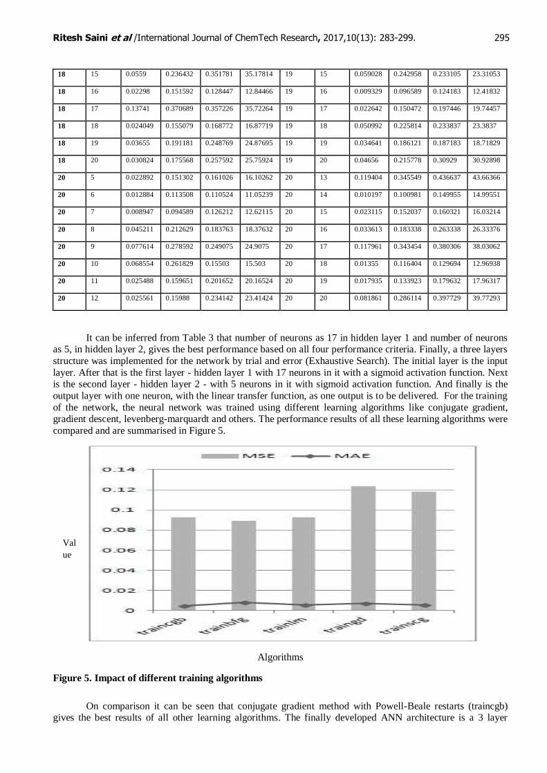
output layer with one neuron, with the linear transfer function, as one output is to be delivered. For the training

of the network, the neural network was trained using different learning algorithms like conjugate gradient, gradient descent, levenberg-marquardt and others. The performance results of all these learning algorithms were

compared and are summarised in Figure 5.

Algorithms

Figure 5. Impact of different training algorithms

On comparison it can be seen that conjugate gradient method with Powell-Beale restarts (traincgb) gives the best results of all other learning algorithms. The finally developed ANN architecture is a 3 layer

Val

ue


model with 17-5 neurons in the first and second hidden layers respectively, trained by conjugate gradient

method with Powell-Beale restarts.

5. Results

5.1. Prediction

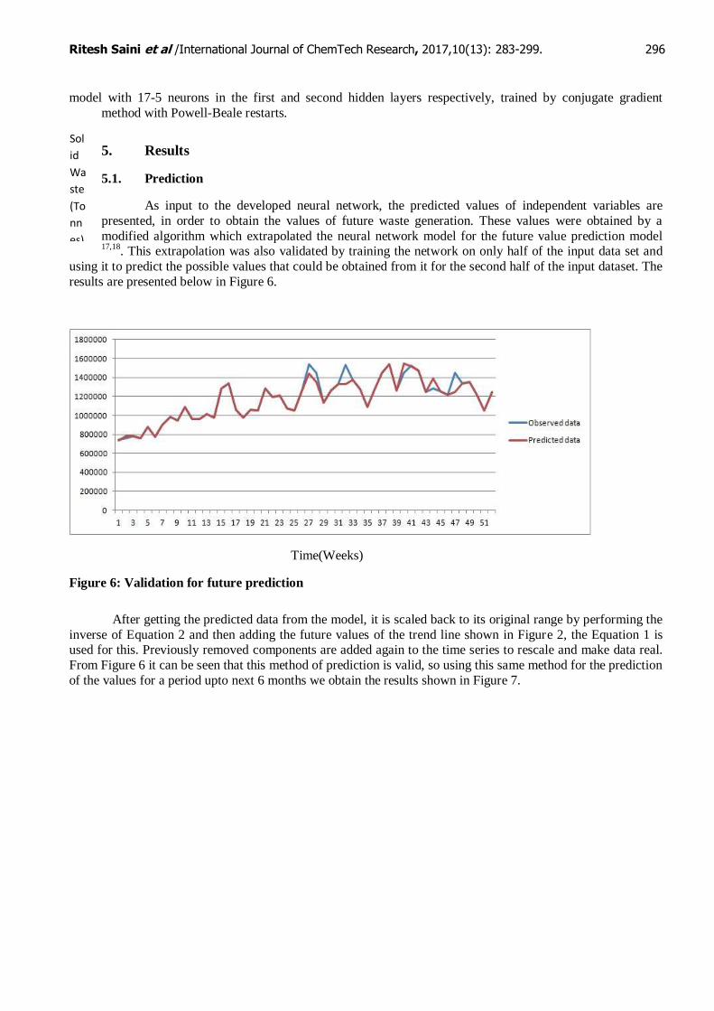
As input to the developed neural network, the predicted values of independent variables are

presented, in order to obtain the values of future waste generation. These values were obtained by a

modified algorithm which extrapolated the neural network model for the future value prediction model 17,18

. This extrapolation was also validated by training the network on only half of the input data set and

using it to predict the possible values that could be obtained from it for the second half of the input dataset. The

results are presented below in Figure 6.

Time(Weeks)

Figure 6: Validation for future prediction

After getting the predicted data from the model, it is scaled back to its original range by performing the

inverse of Equation 2 and then adding the future values of the trend line shown in Figure 2, the Equation 1 is used for this. Previously removed components are added again to the time series to rescale and make data real.

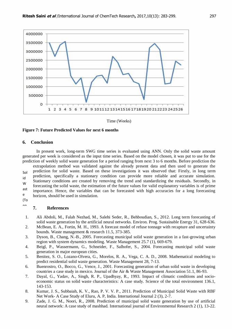
From Figure 6 it can be seen that this method of prediction is valid, so using this same method for the prediction

of the values for a period upto next 6 months we obtain the results shown in Figure 7.

Sol

id

Wa

ste

(To

nn

es)


Time (Weeks)

Figure 7: Future Predicted Values for next 6 months

6. Conclusion

In present work, long-term SWG time series is evaluated using ANN. Only the solid waste amount generated per week is considered as the input time series. Based on the model chosen, it was put to use for the

prediction of weekly solid waste generation for a period ranging from next 3 to 6 months. Before prediction the

extrapolation method was validated against the already present data and then used to generate the prediction for solid waste. Based on these investigations it was observed that: Firstly, in long term

prediction, specifically a stationary condition can provide more reliable and accurate simulation.

Stationary conditions are created by removing the trend and standardizing the residuals. Secondly, in forecasting the solid waste, the estimation of the future values for valid explanatory variables is of prime

importance. Hence, the variables that can be forecasted with high accuracies for a long forecasting

horizon, should be used in simulation.

7. References

1. Ali Abdoli, M., Falah Nezhad, M., Salehi Seder, R., Behboudian, S., 2012. Long term forecasting of solid waste generation by the artificial neural networks. Environ. Prog. Sustainable Energy 31, 628-636.

2. McBean, E. A., Fortin, M. H., 1993. A forecast model of refuse tonnage with recapture and uncertainty

bounds. Waste management & research 11.5, 373-385.

3. Dyson, B., Chang, N.-B., 2005. Forecasting municipal solid waste generation in a fast-growing urban region with system dynamics modeling. Waste Management 25.7 (1), 669-679.

4. Beigl, P., Wassermann, G., Schneider, F., Salhofer, S., 2004. Forecasting municipal solid waste

generation in major european cities. 5. Benitez, S. O., Lozano-Olvera, G., Morelos, R. A., Vega, C. A. D., 2008. Mathematical modeling to

predict residential solid waste generation. Waste Management 28, 7-13.

6. Buenrostro, O., Bocco, G., Vence, J., 2001. Forecasting generation of urban solid waste in developing countries a case study in mexico. Journal of the Air & Waste Management Association 51.1, 86-93.

7. Dayal, G., Yadav, A., Singh, R. P., Upadhyay, R., 1993. Impact of climatic conditions and socio-

economic status on solid waste characteristics: A case study. Science of the total environment 136.1,

143-153. 8. Kumar, J. S., Subbaiah, K. V., Rao, P. V. V. P., 2011. Prediction of Municipal Solid Waste with RBF

Net Work- A Case Study of Eluru, A. P, India. International Journal 2 (3), 2-7.

9. Zade, J. G. M., Noori, R., 2008. Prediction of municipal solid waste generation by use of artificial neural network: A case study of mashhad. International journal of Environmental Research 2 (1), 13-22.

Sol

id

W

ast

e

(To

nn

es)


10. Noori, R., Karbassi, A., Sabahi, M. S., 2010. Evaluation of pca and gamma test techniques on ann

operation for weekly solid waste prediction. Journal of Environmental Management 91 (3), 767-771.

11. Noori, R., Ali, M., Farokhnia, A., Abbasi, M., 2009. Results uncertainty of solid waste generation forecasting by hybrid of wavelet transform-anfis and wavelet transform-neural network. Expert

Systems With Applications 36 (6), 9991-9999.

12. Noori, R., Abdoli, M. A., Ghasrodashti, A. A., Zade, J. G., 2009. Prediction of municipal solid waste

generation with combination of support vector machine and principal component analysis: A case study of mashhad. Environmental progress & sustainable energy 28.2, 249-258.

13. Karaca, F., Ozkaya., B., 2006. Nn-leap: A neural network-based model for controlling leachate flow-

rate in a municipal solid waste landfill site. Environmental Modelling& Software 21.8, 1190-1197. 14. Chen, H.-W., Chang, N.-B., 2000. Prediction analysis of solid waste generation based on grey fuzzy

dynamic modeling. Resources, Conservation and Recycling 29, 118.

15. Shahabi, H., Khezri, S., Ahmad, B. B., Zabihi, H., 2012. Application of artificial neural network in prediction of municipal solid waste generation (case study: Saqqez city in kurdistanprovince )

department of geoinformatics , faculty of geo information and real estate. Neural Networks 20 (2), 336-

343.

16. Noori, R., Abdoli, M. A., Zade, J. G., Samieifard, R., 2009. Comparison of neural network and principal component- regression analysis to predict the solid waste generation in tehran 38 (1), 74-84.

17. Cigizoglu, H. K., 2003. Estimation, forecasting and extrapolation of river flows by artificial neural

networks. Hydrological Sciences 48 (September 2013), 349-361. 18. Shamshiry, E., Mokhtar, M. B., Komoo, I., Hashim, H. S., Nadi, B., Abdulai, A.-m., Nikbakht, M.,

2012. Application of artificial neural network method and landfill leachate pollution index for

prediction of solid waste generation and evaluation in tropical area. International forestry and Environment Symposium 17.

*****


Extra page not to be printed.

For your Research References Requirements-

Log on to www.sphinxsai.com

*****

http://www.sphinxsai.com/

Documents

Futuristic Projection of Solid Waste Generation in ...283-299)V10N13CT.pdf · Futuristic Projection of Solid Waste Generation in Dehradun City of Uttarakhand using Supervised Artificial