Future Mobile Communications: - LTE Radio Scheduler ... · domain scheduler 6/25 ComNets ... eNodeB per UE Buffers MAC-QoS-Class-1 HARQ MAC-QoS-Class-2 MAC-QoS-Class-3 ... LTE-Uu

Future Mobile Communications:LTE Radio Scheduler Analytical Modeling

Dr. Yasir Zaki

New York University Abu Dhabi (NYUAD)FFV Workshop 2013

15th of March 2013

1/251/25

ComNetsCommunication Networks

Overview

1 Introduction

2 LTE Radio Scheduler

3 LTE Scheduler Analytical Models

4 Conclusion

2/252/25


Long Term Evolution (LTE)LTE is the newest 3GPP1 standard (Release 8)

UE

eNodeB

MME

S-GW

HSS

PDN

GW

PCRF

Uu

S1-U

S1-MME

S6a

S11 Gx

Rx

S5/S8

eNodeB

UE E-UTRAN EPC Services

IP connectivity Layers, The EPS

Service connectivity Layer

User plane

Control plane

SGi

Operator’s

IP services

(e.g. IMS, PSS)

The main motivation of the work presented here is the analyticalmodeling of the LTE QoS aware radio scheduler.And to validate our simulation results by comparing it to the analyticalresults.

13rd Generation Partnership Project

3/253/25


LTE OPNET Simulation Model

Application

configProfile

configMobility &

Channel

Global UE

Database

Remote_Server

IPcloud

PDN_GW aGW

eNB1

eNB2

UE1 UE2 UE3 UE4 UE5

UE6 UE7 UE8 UE9 UE10





Remote_Server

IPcloudPDN_GW

aGW

R2

1 2 3

4 5 6

7 8 9

10 11 12

13 14 15

16 17 18

19 20 21

22 23 24

25 26 27

28 29 30

31 32 33

34 35 36

Cell 1

Cell 2

Cell 3

R2

R3

eNB1

R1

eNB2

eNB3

eNB4

Application

TCP/UDP

IP

PDCP

RLC

MAC

PHY

RLC

MAC

PHY

UDP

IP

L2

L1

UDP

IP

L2

L1

UDP

IP

L2

L1

UDP

IP

L2

L1

GTP

IP

L2

L1

Application

TCP/UDP

IP

L2

L1

Relay

PDCPGTP

Relay

GTPGTP

4/254/25


LTE Physical Resource StructureResources in LTE consist of both: time and frequency dimensions

The smallest resource the scheduler can allocate is called aPhysical Resource Block (PRB).A PRB consists of the following:

72 OFDM symbols in the time domain12 sub-carriers in the frequency domain

0

1

2

3

4

5

6

1 S

lot

7 S

ymb

ols

1 2 3 4 5 6 7 8 9 10 11

Resource Block 0

Resource Block 1

Resource Block 2

Resource Block N1

Slo

t7

Sym

bo

ls

Resource Block 3

180 kHz 15 kHz x 12 sub-

carriers15 kHzSymbols

Resource Element

Sub-Carriers

N represents the maximum number of resource blocks

which depend on the defined spectrum/bandwidth

26 or 7 symbols depending on the length of the cyclic prefix

5/255/25


LTE Dynamic Packet Scheduling

The packet scheduling is divided into two different stages:Time Domain Scheduler (TDS): deals with QoS requirements anduser/bearer prioritizationFrequency Domain Scheduler (FDS): deals with spectrumallocation and multi-user diversity exploitation

Time Domain Scheduling

Frequency Domain

Scheduling

Buffer informationQoS informationLink Adaptation

HARQ information...

bearers for FDS

Time Domain Updates

Schedule bearers

In LTE literature such a split is called decoupled time and frequencydomain scheduler

6/256/25


Time Domain Scheduler TDSTwo of the classical TDS schedulers are:

Blind Equal Throughput (BET): give a fair chance of resources so thatusers can achieve similar throughput

Maximum Throughput (MaxT): maximize the cell/system throughput byscheduling users with the best channel conditions

The TDS prioritization is done by calculating the priority factor.

P BETk (t ) = argmaxk

[1

θk [t ]

]= BET TD priority factor

PMaxTk (t ) = argmaxk [SINRk [t ]] = MaxT TD priority factor

θk [t ] is the normalized average throughput of bearer k ranging between 0 and 1

SINRk [t ] is the instantaneous SINR value of bearer k

7/257/25


Frequency Domain Scheduler FDS

Distributes the radio resources (PRBs) among the highest prioritybearers obtained from the TDS

Exploits the multi-user diversity and tries to enhance the overallspectral efficiencyThe FDS used in this work is an optimized round robin scheduler

Serves first strictly the GBR3 bearersServes the highest ψ4 nonGBR priority bearers with the remainingresourcesSchedules the PRBs using an iterative approach

3Guaranteed Bit Rate4ψ is chosen to be 5 in this work

8/258/25


Optimized Service Aware Scheduler

The proposed OSA scheduler provides:

QoS guarantees

Fairness among users

System performance maximization

eNodeB per UE Buffers

MAC-QoS-Class-1

HARQ

MAC-QoS-Class-2

MAC-QoS-Class-3

MAC-QoS-Class-4

MAC-QoS-Class-5

TDS FDS

QCI Classification Time-Domain Scheduling

Frequency-Domain Scheduling

Cla

ssif

ier PRB

assignmentGBR

Candidate List

nonGBR Candidate List

9/259/25


OSA Scheduler: TDS and FDS

The OSA TDS priority factor is:

P nonGBR−OSAk (t ) = argmaxk

[WQoS j ×

γk [t ]

θk [t ]

]

WQoS j is the QoS weight of the j th QoS class

θk [t ] is the normalized EMA5 throughput of bearer kγk [t ] is the normalized EMA channel condition of bearer k

The OSA serves the GBR bearers (i.e., VoIP) with strict prioritybefore the non-GBR bearers

The OSA FDS is an optimized round robin scheduler

5Exponential Moving Average

10/2510/25


LTE Scheduler Analytical Models

The presented model is an extension of the model found in [1]

The scheduler has a fixed amount of PRBs to distribute amongactive UEs every TTI 6

The UEs have different SINRSupport different Modulation and Coding Schemes (MCS)

[1] S. Doirieux, ... “An efficient analytical model for the dimensioning of WiMAX networks supporting multi-profile best efforttraffic”, Computer Communications, Volume 33, Issue 10, 15 June 2010

6Transmission Time Interval = 1ms

11/2511/25


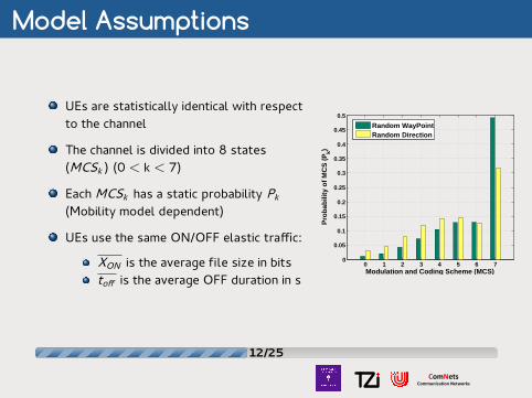
Model Assumptions

UEs are statistically identical with respectto the channel

The channel is divided into 8 states(MCSk ) (0 < k < 7)

Each MCSk has a static probability Pk

(Mobility model dependent)

UEs use the same ON/OFF elastic traffic:

XON is the average file size in bitstoff is the average OFF duration in s

0 1 2 3 4 5 6 70

0.05

0.1

0.15

0.2

0.25

0.3

0.35

0.4

0.45

0.5

Modulation and Coding Scheme (MCS)

Pro

bab

ility

of

MC

S (

Pk)

Random WayPointRandom Direction

12/2512/25


General Analytical Model

The model is based on the Continuous Time Markov Chain (CTMC)n: Markov chain state representing the number of active UEs in a TTIN: total number of UEs in the system

The resulting CTMC consists of N+1 statesArrival transition is performed with rate (N − n )λ with λ = 1/toffDeparture transition is performed with a generic rate µ(n )

10 2

Nλ (N-1)λ λ

µ(1) µ(2) µ(N)

nn-1 n+1

(N-n+1)λ (N-n)λ

µ(n) µ(n+1)

N

(n0, n1, …, nk)Σi ni = n

13/2513/25


LTE Frequency Domain Scheduler

The FDS is a round robin scheduler

It serves up to ψ=5 users per TTI

This means, that the UEs served per TTI are equal to η:

η = min [n − n0, ψ]

with n being the number of active users in a TTI, and n0 is thenumber of users in outage7

7User is in bad channel condition that does not allow any transmission

14/2514/25


Steady State Probability

The steady state probability π(n ) can be calculated from:

π · Q = 0 (1)

π=[π0, π1, ...πN ] and∑

i πi = 1Q is the infinitesimal generator matrix

According to Little’s law, the average ON period duration tON8 is:

ton =

∑Nn=1 nπ(n )∑N

n=1(N − n + 1)λ · π(n )

8tON is the duration of an active transfer, or file download time

15/2515/25


Departure Rate µ(n )

µ(n ) =

∑(n ,...,n )(n0,...,nK )=(0,...,0)|

n0+...+nK=nn0 6=n

TBS (n0, ..., nK )(

nn0, ..., nK

)[∏Kk=0 P

nkk

]Xon · TTI

Xon is the average file size of the ON period(n

n0, ..., nK

)is the multinomial coefficient

Pk is the stationary probability of MCSk

nk is the number of active users in MCSk

TBS (n0, ..., nK ) is the total number of bits transmitted for all servedusers under a certain combination (n0, ..., nK )

16/2516/25


TBS (n0, ..., nK )

TBS (n0, ..., nK ) =∑

i=[i1,...,iη]

TBSi (η) (2)

η is the number of users served under (n0, ..., nK )

[i1, ..., iη] represents the index of the chosen η users out of the nactive users considered for scheduling within a TTI

TBSi (η) denotes the number of bits of user i using his MCS

the choice of the η users is determined by the TD scheduler.

17/2517/25


Choosing η UEs Procedure- MaxT chooses the η UEs with the highest MCS

MCS0 MCS1 MCS2 MCS3

n0 n1 n2 n3

Find η UEs

MCS4 MCS5 MCS6 MCS7

n4 n5 n6 n7

- BET chooses the η UEs from the MCS that achieves the avg. throughput:

MCS0 MCS1 MCS2 MCS3

n0 n1 n2 n3

Find (η-1) UEs

MCS4 MCS5 MCS6 MCS7

n4 n5 n6 n7

Find 1 UE

- OSA chooses the η UEs from the MCS as follows:

MCS0 MCS1 MCS2 MCS3

n0 n1 n2 n3

Find (η-1) UEs

MCS4 MCS5 MCS6 MCS7

n4 n5 n6 n7

Find 1 UE

AverageThroughput =K∑

k=1TBSk · Pk

0 1 2 3 4 5 6 70

0.05

0.1

0.15

0.2

0.25

0.3

0.35

0.4

0.45

0.5

Modulation and Coding Scheme (MCS)P

rob

abili

ty o

f M

CS

(P

k)

Random WayPointRandom Direction

18/2518/25


Two Classes Model

The single class model is extendedinto a two dimensional Markov Chain,with state (i,j)

i represents the number of UEswithin class 1j represents the number of UEswithin class 2

The combinations within each statewill increase to:(i0, i1, i2, i3, i4, i5, i6, i7, j0, j1, j2, j3, j4, j5, j6, j7)where

∑r ir = N1 and =

∑r jr = N2

0,1

1,1

0,0

1,0

0,2

1,2

0,N2

1,N2

N1,1N1,0 N1,2 N1,N2

N2λ2 (N2-1)λ2 (N2-2)λ2 λ2

µ2(N1,1) µ2(N1,2) µ2(N1,3) µ2(N1,N2)

N1λ 1

λ 1(N

1-1)λ

1

µ1(1,0)

µ1(2,0)

µ1(N

1,0)

19/2519/25


Three Classes Model

Similary the single class model canbe extended into a three dimensionalMarkov Chain, with state (i,j,z)

i represents the number of UEswithin class 1j represents the number of UEswithin class 2z represents the number ofUEs within class 3

The combinations within each statewill increase to:(i0, i1, i2, i3, i4, i5, i6, i7, j0, j1, j2, j3, j4, j5, j6, j7, z0, z1, z2, z3, z4, z5, z6, z7)where

∑r ir = N1 and

∑r jr = N2

and∑

r zr = N3

20/2520/25


Scenarios Configuration

General parameter ValueBandwidth (# PRBs) 5 MHz (i.e., 25 PRBs)Radio QoS weights WQoS 1=5, WQoS 2=2 and WQoS 3=1Traffic model FTP with different IATs:

uniform (0, 30) s, uniform (15, 45) s,uniform (30, 60) s and uniform (45, 75) s

Simulation run time 8000 s, 10 seeds with 95% confidence interval

Analysis Class1 Class2 Class3

MaxT 10 UEs with5, 10 and 15 MByte

3 UEs with 6 UEs withw-MaxT 5 MByte 10 MByte

3 UEs with 3 UEs with 3 UEs withw-MaxT 5 MByte 10 MByte 15 MByte

21/2521/25


Average FTP Download Time: MaxT

15 30 45 600

20

40

60

80

100

120

140

160

Inter−arrival−time IAT (sec)

Dow

nloa

d tim

e (s

ec)

MaxT Average FTP download time (10UEs scenario)

5MB simulation5MB analytical10MB simulation10MB analytical15MB simulation15MB analytical

22/2522/25


Average FTP Download Time: w-MaxT

15 30 45 600

10

20

30

40

50

60

70

Inter−arrival−time IAT (sec)

Dow

nloa

d tim

e (s

ec)

w−MaxT Average FTP download time

class1 simulationclass1 analyticalclass2 simulationclass2 analytical

23/2523/25


Average FTP Download Time: w-MaxT

15 30 45 600

10

20

30

40

50

60

70

80

90

100

Iner−arrival−time IAT (sec)

Dow

nloa

d tim

e (s

ec)

w−MaxT Average FTP download time

class1 simulationclass1 analytical

class2 simulation

class2 analytical

class3 simulationclass3 analytical

24/2524/25


Conclusion and Outlook

The proposed analytical model shows very accurate resultscompared to the simulation results

The model can support up to three different QoS classes

The analytical model only requires a couple of minutes to run (muchfaster than simulations)The model can be extended to:

support more QoS classesa GBR class can also be modeledother types of TDS can also be modeled

25/2525/25


Thanks for Listening

Backup issues

LTE QoS bearers

3GPP QoS bearer classification

Channel dependent scheduling

Channel model

Analytical model scaling

Analytical model TBS(n)

Analytical model Q-matrix

BACKUP

3GPP QoS Bearer Classification

UE eNodeB S-GW P-GW Peer Entity

E-UTRAN EPC Internet

End-to-End Service

External BearerEPS Bearer

S5/S8 BearerS1 BearerRadio Bearer

LTE-Uu S1 S5/S8 SGi

back

LTE QoS BearersQCI Bearer type Priority Packet delay Packet error Example services

budget (ms) loss rate

1 GBR 2 100 10−2 Conversational voice2 GBR 4 150 10−3 Conversational video

(live streaming)3 GBR 5 300 10−6 Non-conversational

video (buffered streaming)4 GBR 3 50 10−3 Real time gaming5 non-GBR 1 100 10−6 IMS signaling6 non-GBR 7 100 10−3 Voice,

video (live streaming),interactive gaming

7 non-GBR 6 300 10−6 Video (buffered streaming)8 non-GBR 8 300 10−6 TCP based (e.g., www,

e-mail, chat, FTP, p2p)9 non-GBR 9 300 10−6

Nine predefined QoS classesfour Guaranteed Bit Rate (GBR)five non Guaranteed Bit Rate (nonGBR)

Operators are free to choose their own classificationback

Channel Dependent Scheduling

User #2 scheduled

Frequency

User #1 channel

User #1 scheduled

Time

User #2 channel

back

Channel Model

Path loss:

128.1+ 37.6 · log10(distance )

Correlated slow fading:Log-normal distributed

Fast fading:Jakes-like methodTwo extended ITU channel models

Extended pedestrian AExtended vehicular A

20002004

20082012

20162020

0

200

400

600

800

1000−40

−30

−20

−10

0

10

20

30

Frequency (MHz)time (msec)

Fast fading (dB)

back

Steady State Probability

Another solution wiil be to use the closed loop solution from thebirth-and-death process of the Markov chain:

π(n ) =

[n∏

i+1

(N − i + 1)λµ(i )

]π(0)

π(0) is obtained by normalization

back

TBS (2)if we have two active UEs i.e. n=2those two users can be at any MCS (from MCS0 to MCS7)if we represent the number of users in each MCSk by nk we get:(n0, n1, n2, n3, n4, n5, n6, n7) with n0 + ...+ n7 = nthen we have the following possible combinations

back

TBS (2)

TBS (2) =(2,...,2)∑

(n0,...,nK )=(0,...,0)|n0+...+nK=0

n0 6=2

TBS (n0, ..., nK )(

2n0, ..., nK

)[K∏

k=0

P nkk

]

(3)

back

Q Infinitesimal Generator Matrix

0,1

1,1

0,0

1,0

0,2

1,2

0,N2

1,N2

N1,1N1,0 N1,2 N1,N2

N2λ2 (N2-1)λ2 (N2-2)λ2 λ2

µ2(N1,1) µ2(N1,2) µ2(N1,3) µ2(N1,N2)

N1λ 1

λ 1(N

1-1)λ

1

µ1(1,0)

µ1(2,0)

µ1(N

1,0)

N1,1N1,0 N1,2 N1,N20,1 1,10,0 1,00,2 1,20,N2 1,N2

back

Q Infinitesimal Generator Matrix

(0,0) (0,1) (0,2) (0,3) (0,4)

(0,0)

(1,0) (1,1) (1,2) (1,3) (1,4) (2,0) (2,1) (2,2) (2,3) (2,4)

(0,1)

(0,2)

(0,3)

(0,4)

(1,0)

(1,1)

(1,2)

(1,3)

(1,4)

(2,0)

(2,1)

(2,2)

(2,3)

(2,4)

4λ1 2λ2

μ1

(0,1)3λ1 2λ2

μ1

(0,2)2λ1 2λ2

μ1

(0,3)λ1 2λ2

μ1

(0,4)0 2λ2

μ2

(1,0)

μ1

(1,0)4λ1 λ2

μ2

(1,1)

μ1

(1,1)3λ1 λ2

μ2

(1,2)

μ1

(1,2)2λ1 λ2

μ2

(1,3)

μ1

(1,3)λ1 λ2

μ2

(1,4)

μ1

(1,4)0 λ2

μ2

(2,0)

μ1

(2,0)4λ1

μ2

(2,1)

μ1

(2,1)3λ1

μ2

(2,2)

μ1

(2,2)2λ1

μ2

(2,3)

μ1

(2,3)λ1

μ2

(2,4)

μ1

(2,4)

Markov chain state (i,j)

Ma

rko

v c

ha

in s

tate

(i,j)

Q (i , i ) = −∑j

Q (i , j )

back

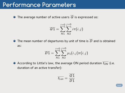
Performance ParametersThe average number of active users Q is expressed as:

Q 1 =i=0∑N 1

j=0∑N 2

iπ(i , j )

The mean number of departures by unit of time is D and is obtainedas:

D 1 =i=0∑N 1

j=0∑N 2

µ1(i , j )π(i , j )

According to Little’s law, the average ON period duration tON (i.e.duration of an active transfer):

t1on =Q 1D 1

back

Departure Rate µ1(i , j )

µ1(i , j ) = TBS 1(i ,j )X 1on ·TTI

TBS 1(i , j ) is the average amount of bits sent by all served UEs in aTTI

X 1on is the average file size of class 1 UEs

TTI is the Transmission Time Interval (1ms)

back

Generic Average Bit Rate TBS 1(i , j )

TBS 1(i , j ) =(i ,...,i ,j ,...,j )∑

(i0,...,iK ,j0,...,jK )=(0,...,0)|i0+...+iK=ij0+...+jK=j

i0 6=i with j0 6=j

i !j !TBS 1(i0, ..., iK , j0, ..., jK )

[K∏

k=0

P ikk P jk

k

ik !jk !

]

Pk is the stationary probability of MCSk

ik is the number of class 1 active users in MCSk

jk is the number of class 2 active users in MCSk

TBS 1(i0, ..., iK , j0, ..., jK ) is the total bits transmitted for all served UEsunder a certain combination (i0, ..., iK , j0, ..., jK )

back

TBS 1(i0, ..., iK , j0, ..., jK )

TBS 1(i0, ..., iK , j0, ..., jK ) =∑

r=[r1,...,rδ1]

TBSr (η)

rδ1 + rδ2 = η

r is a vector representing the indices of the served users in class1

rδ1 is the number of users served in class1.

TBS 2(i0, ..., iK , j0, ..., jK ) can be calculated similarly

back

choosing eta Users

AverageThroughput =K∑

k=1

TBSk · Pk

K is the number of MCSs

TBSk is the transport block size using MCSk

Pk is the static probability of MCSk

Avg. throughput for RWP is MCS5

Avg. throughput for RD is MCS4

back

Analytical Model ScalingThese measurements were performed in MATLAB using a server with AMD Phenom(tm) 9850 Quad-Core Processor 2.50 GHz,8.00 GB of RAM, and 64-bit Windows 7 OS.

back

Model Number of UEs Combinations Run time

1-D 10 UEs 19448 2 seconds20 UEs 888029 79 seconds

2-D (3,6) UEs 205919 49 seconds3-D (2,3,5) UEs 3421440 13 minutes ??

1−D 2−D 3−D0

0.5

1

1.5

2

2.5

3

3.5

4x 10

6

# of Combinations

Documents

Future Mobile Communications: - LTE Radio Scheduler ... · domain scheduler 6/25 ComNets ... eNodeB per UE Buffers MAC-QoS-Class-1 HARQ MAC-QoS-Class-2 MAC-QoS-Class-3 ... LTE-Uu