Further calculus - University of London · Further calculus A. Ostaszewski, J.M. Ward MT2176, 2790176 2012 Undergraduate study in ... + Ostaszewski, A. Advanced mathematical methods

Further calculusA. Ostaszewski, J.M. WardMT2176, 2790176

2012

Undergraduate study in Economics, Management, Finance and the Social Sciences

This is an extract from a subject guide for an undergraduate course offered as part of the University of London International Programmes in Economics, Management, Finance and the Social Sciences. Materials for these programmes are developed by academics at the London School of Economics and Political Science (LSE).

For more information, see: www.londoninternational.ac.uk

This guide was prepared for the University of London International Programmes by:

A. Ostaszewski, Department of Mathematics, The London School of Economics and Political Science.

J.M. Ward, Department of Mathematics, The London School of Economics and Political Science.

This is one of a series of subject guides published by the University. We regret that due to pressure of work the authors are unable to enter into any correspondence relating to, or aris-ing from, the guide. If you have any comments on this subject guide, favourable or unfavour-able, please use the form at the back of this guide.

University of London International ProgrammesPublications OfficeStewart House32 Russell SquareLondon WC1B 5DNUnited Kingdom

www.londoninternational.ac.uk

Published by: University of London

© University of London 2012

The University of London asserts copyright over all material in this subject guide except where otherwise indicated. All rights reserved. No part of this work may be reproduced in any form, or by any means, without permission in writing from the publisher.

We make every effort to contact copyright holders. If you think we have inadvertently used your copyright material, please let us know.

Contents

Contents

1 Introduction 1

1.1 This subject . . . . . . . . . . . . . . . . . . . . . . . . . . . . . . . . . . 1

1.2 Reading . . . . . . . . . . . . . . . . . . . . . . . . . . . . . . . . . . . . 2

1.3 Online study resources . . . . . . . . . . . . . . . . . . . . . . . . . . . . 3

1.3.1 The VLE . . . . . . . . . . . . . . . . . . . . . . . . . . . . . . . 4

1.3.2 Making use of the Online Library . . . . . . . . . . . . . . . . . . 5

1.4 Using this subject guide . . . . . . . . . . . . . . . . . . . . . . . . . . . 5

1.5 Examination advice . . . . . . . . . . . . . . . . . . . . . . . . . . . . . . 5

1.6 The use of calculators . . . . . . . . . . . . . . . . . . . . . . . . . . . . . 6

2 Limits 7

2.1 Limits . . . . . . . . . . . . . . . . . . . . . . . . . . . . . . . . . . . . . 7

2.1.1 Limits at infinity . . . . . . . . . . . . . . . . . . . . . . . . . . . 8

2.1.2 Limits at a point . . . . . . . . . . . . . . . . . . . . . . . . . . . 19

2.2 Some useful results that involve limits . . . . . . . . . . . . . . . . . . . . 28

2.2.1 Continuity . . . . . . . . . . . . . . . . . . . . . . . . . . . . . . . 28

2.2.2 Differentiability . . . . . . . . . . . . . . . . . . . . . . . . . . . . 29

2.2.3 Taylor series and Taylor’s theorem . . . . . . . . . . . . . . . . . 31

2.2.4 L’Hopital’s rule . . . . . . . . . . . . . . . . . . . . . . . . . . . . 34

Learning outcomes . . . . . . . . . . . . . . . . . . . . . . . . . . . . . . . . . 38

Solutions to activities . . . . . . . . . . . . . . . . . . . . . . . . . . . . . . . . 38

Exercises . . . . . . . . . . . . . . . . . . . . . . . . . . . . . . . . . . . . . . . 46

Solutions to exercises . . . . . . . . . . . . . . . . . . . . . . . . . . . . . . . . 47

3 The Riemann integral 53

3.1 The Riemann integral . . . . . . . . . . . . . . . . . . . . . . . . . . . . . 53

3.1.1 Lower and upper estimates of an area . . . . . . . . . . . . . . . . 54

3.1.2 Getting better lower and upper estimates . . . . . . . . . . . . . . 60

3.1.3 The definition of the Riemann integral . . . . . . . . . . . . . . . 63

3.1.4 What happens if the integrand isn’t continuous? . . . . . . . . . . 66

3.1.5 Some properties of the Riemann integral . . . . . . . . . . . . . . 71

i

Contents

3.2 The Fundamental Theorem of Calculus . . . . . . . . . . . . . . . . . . . 72

3.2.1 Motivating the FTC . . . . . . . . . . . . . . . . . . . . . . . . . 72

3.2.2 Notation: Dummy variables . . . . . . . . . . . . . . . . . . . . . 75

3.2.3 The relationship between integration and differentiation . . . . . . 76

3.2.4 Some applications of the FTC . . . . . . . . . . . . . . . . . . . . 77

3.2.5 An extension of the FTC . . . . . . . . . . . . . . . . . . . . . . . 79



Exercises . . . . . . . . . . . . . . . . . . . . . . . . . . . . . . . . . . . . . . . 93


4 Improper integrals 99

4.1 Improper integrals . . . . . . . . . . . . . . . . . . . . . . . . . . . . . . 99

4.1.1 Improper integrals of two kinds, and a third kind . . . . . . . . . 100

4.1.2 Some further thoughts on improper integrals . . . . . . . . . . . . 102

4.2 Tests for convergence and divergence . . . . . . . . . . . . . . . . . . . . 106

4.2.1 The Direct Comparison Test . . . . . . . . . . . . . . . . . . . . . 107

4.2.2 The Limit Comparison Test . . . . . . . . . . . . . . . . . . . . . 111

4.2.3 Variable sign integrands . . . . . . . . . . . . . . . . . . . . . . . 121



Exercises . . . . . . . . . . . . . . . . . . . . . . . . . . . . . . . . . . . . . . . 129


5 Double integrals 135

5.1 Double integrals . . . . . . . . . . . . . . . . . . . . . . . . . . . . . . . . 135

5.1.1 Volumes over rectangular bases . . . . . . . . . . . . . . . . . . . 136

5.1.2 Defining double integrals in terms of volumes . . . . . . . . . . . 137

5.1.3 Motivating Fubini’s theorem . . . . . . . . . . . . . . . . . . . . . 139

5.1.4 Fubini’s theorem . . . . . . . . . . . . . . . . . . . . . . . . . . . 141

5.1.5 Volumes over other bases . . . . . . . . . . . . . . . . . . . . . . . 143

5.2 Change of variable techniques . . . . . . . . . . . . . . . . . . . . . . . . 152

5.3 Improper double integrals . . . . . . . . . . . . . . . . . . . . . . . . . . 162



Exercises . . . . . . . . . . . . . . . . . . . . . . . . . . . . . . . . . . . . . . . 179

ii

Contents


6 Manipulation of integrals 187

6.1 The manipulation of proper integrals . . . . . . . . . . . . . . . . . . . . 187

6.1.1 Joint continuity . . . . . . . . . . . . . . . . . . . . . . . . . . . . 188

6.1.2 The manipulation rules for proper integrals . . . . . . . . . . . . . 191

6.1.3 Applications of the rules for manipulating proper integrals . . . . 194

6.2 The manipulation of improper integrals . . . . . . . . . . . . . . . . . . . 197

6.2.1 Dominated convergence . . . . . . . . . . . . . . . . . . . . . . . 198

6.2.2 The manipulation rules for improper integrals . . . . . . . . . . . 205

6.2.3 Using the rules for manipulating improper integrals . . . . . . . . 206



Exercises . . . . . . . . . . . . . . . . . . . . . . . . . . . . . . . . . . . . . . . 216


7 Laplace transforms 221

7.1 What is a Laplace transform? . . . . . . . . . . . . . . . . . . . . . . . . 221

7.1.1 Some properties of the Laplace transform . . . . . . . . . . . . . . 223

7.1.2 Extending our view of Laplace transforms . . . . . . . . . . . . . 230

7.2 Using Laplace transforms . . . . . . . . . . . . . . . . . . . . . . . . . . . 233

7.2.1 Solving ODEs with constant coefficients . . . . . . . . . . . . . . 233

7.2.2 Convolutions . . . . . . . . . . . . . . . . . . . . . . . . . . . . . 236



Exercises . . . . . . . . . . . . . . . . . . . . . . . . . . . . . . . . . . . . . . . 251


A Sample examination paper 257

B Solutions to the sample examination paper 261

iii

Contents

iv

1

Chapter 1

Introduction

In this very brief introduction, we aim to give you an idea of the nature of this subjectand to advise you on how best to approach it. We give general information about thecontents and use of this subject guide, and on recommended reading and how to use thetextbooks.

1.1 This subject

Calculus, as studied in this 200 course, is primarily the study of integrals of functions ofone and two variables.

Our approach here is not just to help you acquire proficiency in techniques andmethods, but also to help you understand some of the theoretical ideas behind these.For example, after completing this course, you will hopefully understand how certainkinds of definite integral are defined and how to deal with integrals where the integrandis a function of two variables.

Aims of the course

The broad aims of this course are:

to enable students to acquire skills in the methods of calculus, as required for theiruse in further mathematics subjects and economics-based subjects;

to prepare students for further courses in mathematics and/or related disciplines.

However, as emphasised above, we do also want you to understand why certain methodswork: this is one of the ‘skills’ that you should acquire. Indeed, the examination will notsimply test your ability to perform routine calculations, it will also probe yourknowledge and understanding of the principles that underlie the material.

Learning outcomes

We now state the broad learning outcomes of this course, as a whole. At the end of thiscourse and having completed the essential reading and activities, you should be able to:

1

1 1. Introduction

demonstrate knowledge of the subject matter, terminology, techniques andconventions covered in the subject;

demonstrate an understanding of the underlying principles of the subject;

demonstrate the ability to solve problems involving an understanding of theconcepts.

There are a couple of things that we should stress at this point. Firstly, note theintention that you will be able to solve unseen problems. This means simply that youwill be expected to be able to use your knowledge and understanding of the material tosolve problems that are not completely standard. This is not something you shouldworry unduly about: all courses in mathematics expect this, and you will never beexpected to do anything that cannot be done using the material of this course.Secondly, we expect you to be able to ‘demonstrate knowledge and understanding’ andyou might well wonder how you would demonstrate this in the examination. Well, it isprecisely by being able to grapple successfully with unseen, non-routine, questions thatyou will indicate that you have a proper understanding of the topic.

Topics covered

Descriptions of the topics to be covered appear in the relevant chapters. However, it isuseful to give a brief overview at this stage.

We start by introducing the limit of a function of one variable and, in particular, howthis can be used to define what it means to say that a function is continuous. We thenintroduce the Riemann integral and explain its relationship to differentiation via theFundamental Theorem of Calculus. This leads on to a discussion of improper integralsand, in particular, some tests that we can use to determine whether such integrals areconvergent or divergent. We then turn our attention to functions of two variables, inparticular, how we can integrate such functions over certain regions and how we canmanipulate such integrals. We then discuss Laplace transforms and some of theirimportant applications.

Throughout this subject guide, the emphasis will be on the theory as much as on themethods. That is to say, our aim in this subject is not only to provide you with someuseful techniques and methods from calculus, but to also enable you to understand whythese techniques work.

1.2 Reading

There are many books that would be useful for this subject. We recommend two inparticular, and a couple of others for additional, further reading. (You should note,however, that there are very many books suitable for this course. Indeed, almost anytext on first-year university calculus will cover the majority of the material.)

Textbook reading is essential as textbooks will provide you with more in-depthexplanations than you will find in this subject guide, and they will also provide manymore examples to study and exercises to work through. The books listed are the oneswe have referred to in this subject guide.

2

11.3. Online study resources

Essential reading

Detailed reading references in this subject guide refer to the editions of the settextbooks listed below. New editions of one or more of these textbooks may have beenpublished by the time you study this course. You can use a more recent edition of anyof the books; use the detailed chapter and section headings and the index to identifyrelevant readings. Also check the virtual learning environment (VLE) regularly forupdated guidance on readings.

+ Binmore, K. and J. Davies Calculus: concepts and methods. (Cambridge:Cambridge University Press, 2002) second revised edition [ISBN 9780521775410].

+ Ostaszewski, A. Advanced mathematical methods. (Cambridge: CambridgeUniversity Press, 1991) [ISBN 9780521289641].

Both of these texts, when used wisely, will provide you with a large number of examplesfor you to study and exercises for you to attempt. It is recommended that you purchaseboth of these.

Further reading

Once you have covered the essential reading you are then free to read around thesubject area in any text, paper or online resource. You will need to support yourlearning by reading as widely as possible and by thinking about how these principlesapply in the real world. To help you read extensively, you have free access to the VLEand University of London Online Library (see Section 1.3.2). However, two usefultextbooks that we have referred to in this subject guide are the following.

+ Adams, R.A. and C. Essex Calculus: A complete course. (Toronto: Pearson, 2009)seventh edition [ISBN 9780321549280].

+ Wrede, R. C. and M. Spiegel Schaum’s outline of advanced calculus. (London:McGraw-Hill, 2010) third edition [ISBN 9780071623667].

Adams and Essex (which is merely an example from a large range of very similarcalculus textbooks) is a detailed calculus textbook which contains much material whichis beyond the scope of this course. Wrede and Spiegel contains a brief summary of someof the course material but is useful as it contains a large number of worked examplesand exercises. Both of these texts are suitable as sources of additional explanation,examples and exercises, but they are probably not worth purchasing.

1.3 Online study resources

In addition to the subject guide and the essential reading, it is crucial that you takeadvantage of the study resources that are available online for this course, including theVLE and the Online Library.

3

1 1. Introduction

You can access the VLE, the Online Library and your University of London emailaccount via the Student Portal at

http://my.londoninternational.ac.uk

You should have received your login details for the Student Portal with your officialoffer, which was emailed to the address that you gave on your application form. Youhave probably already logged in to the Student Portal in order to register! As soon asyou registered, you will automatically have been granted access to the VLE, OnlineLibrary and your fully functional University of London email account.

If you forget your login details at any point, please email [email protected] your student number.

1.3.1 The VLE

The VLE, which complements this subject guide, has been designed to enhance yourlearning experience, providing additional support and a sense of community. It forms animportant part of your study experience with the University of London and you shouldaccess it regularly.

The VLE provides a range of resources for EMFSS courses:

Self-testing activities: Doing these allows you to test your own understanding ofsubject material.

Electronic study materials: The printed materials that you receive from theUniversity of London are available to download, including updated reading listsand references.

Past examination papers and Examiners’ commentaries: These provide advice onhow each examination question might best be answered.

A student discussion forum: This is an open space for you to discuss interests andexperiences, seek support from your peers, work collaboratively to solve problemsand discuss subject material.

Videos: There are recorded academic introductions to the subject, interviews anddebates and, for some courses, audio-visual tutorials and conclusions.

Recorded lectures: For some courses, where appropriate, the sessions from previousyears’ Study Weekends have been recorded and made available.

Study skills: Expert advice on preparing for examinations and developing yourdigital literacy skills.

Feedback forms.

Some of these resources are available for certain courses only, but we are expanding ourprovision all the time and you should check the VLE regularly for updates.

4

11.4. Using this subject guide

1.3.2 Making use of the Online Library

The Online Library contains a huge array of journal articles and other resources to helpyou read widely and extensively.

To access the majority of resources via the Online Library at

http://tinyurl.com/ollathens

you will either need to use your University of London Student Portal login details, oryou will be required to register and use an Athens login.

The easiest way to locate relevant content and journal articles in the Online Library isto use the Summon search engine.

If you are having trouble finding an article listed in a reading list, try removing anypunctuation from the title, such as single quotation marks, question marks and colons.

For further advice, please see the online help pages at

www.external.shl.lon.ac.uk/summon/about.php

1.4 Using this subject guide

We have already mentioned that this subject guide is not a textbook. It is importantthat you read textbooks in conjunction with the subject guide and that you tryproblems from the textbooks. The exercises at the end of the main chapters of thissubject guide are a very useful resource and you should try them once you think youhave mastered the material from the chapter. You should really try these exercisesbefore consulting the solutions, as simply reading the solutions provided will not helpyou at all. Sometimes, the solutions we provide will just be an overview of what isrequired, i.e. an indication of how you should answer the questions, but in theexamination, you must always show all of your calculations. It is vital that you developand enhance your problem-solving skills and the only way to do this is to try lots ofexercises.

1.5 Examination advice

Important: the information and advice given here are based on the examinationstructure used at the time this subject guide was written. Please note that subjectguides may be used for several years. Because of this we strongly advise you to alwayscheck both the current Regulations for relevant information about the examination, andthe VLE where you should be advised of any forthcoming changes. You should alsocarefully check the rubric/instructions on the paper you actually sit and follow thoseinstructions.

Remember, it is important to check the VLE for:

Up-to-date information on examination and assessment arrangements for thiscourse.

5

1 1. Introduction

Where available, past examination papers and Examiners’ commentaries for thecourse which give advice on how each question might best be answered.

This course is assessed by a two hour unseen written examination. There are nooptional topics in this subject: you should study them all and this is reflected in thestructure of the examination paper. There are five questions (each worth 20 marks) andall questions are compulsory. A sample examination paper may be found in an appendixto this subject guide.

Please do not think that the questions in your real examination will necessarily be verysimilar to the exercises in this subject guide or those in the sample examination paper.The examination is designed to test you. You will get examination questions unlike thequestions in this subject guide. The whole point of examining is to see whether you canapply your knowledge in familiar and unfamiliar settings. The Examiners (nice peoplethough they are) have an obligation to surprise you! For this reason, it is importantthat you try as many examples as possible from the subject guide and from thetextbooks. This is not so that you can cover any possible type of question theExaminers can think of! It is so that you get used to confronting unfamiliar questions,grappling with them, and finally coming up with the solution.

Do not panic if you cannot completely solve an examination question. There are manymarks to be awarded for using the correct approach or method.

1.6 The use of calculators

You will not be permitted to use calculators of any type in the examination. This is notsomething that you should worry about: the Examiners are interested in assessing thatyou understand the key concepts, ideas, methods and techniques, and will set questionswhich do not require the use of a calculator.

6

2Chapter 2

Limits

Essential reading

(For full publication details, see Chapter 1.)

+ Ostaszewski (1991) Sections 17.4–17.6 and Section 18.8.

Further reading

+ Adams and Essex (2010) Sections 1.2–1.4, parts of Section 2.2, Sections 4.3 and4.9–4.10.

+ Wrede and Spiegel (2010) parts of Chapters 3, 4 and 11.

Aims and objectives

The objectives of this chapter are:

to see what a limit is and how they can be found in a variety of different situations;

to examine the relationship between limits, continuity and differentiability.

Specific learning outcomes can be found near the end of this chapter.

2.1 Limits

We encountered the general idea behind limits in 174 Calculus and, although we usedthe idea there, we never gave a thorough account of what was involved. In this section,we will make the idea behind a limit more precise, but our account will still be fairlyinformal.1 And, once we have done this, we will look at some useful results that involvelimits such as the use of limits to define what it means to say that a function iscontinuous or differentiable. We will also see how our understanding of Taylor series canbe extended by using Taylor’s theorem and we will end this chapter by consideringL’Hopital’s rule which will allow us to calculate some of the ‘trickier’ limits that we willencounter.

1That is, we will say enough to make the idea of a limit precise and see how to calculate limits, butwe will not give a rigorous mathematical treatment of limits like the one you will see in 116 AbstractMathematics.

7

2

2. Limits

2.1.1 Limits at infinity

Limits ‘at infinity’ are concerned with the behaviour of a function, f(x), as x tends toinfinity, a situation we denoted by ‘x→∞’ in 174 Calculus. Indeed, as we saw in thatcourse, this kind of information is useful when we were sketching the graph of a functionbecause it told us what was happening as x gets ‘very large’. In this section, we considerexactly what this kind of limit means and see how we can find such a limit (if it exists)in some straightforward cases.

Finite limits

Suppose that l is a real number and that f(x) is a function, we start by asking what itmeans to say that f(x)→ l as x→∞, i.e. what it means to say that

limx→∞

f(x) = l.

Intuitively, based on what we saw in 174 Calculus, we would want to say that thismeans that the curve y = f(x) has a horizontal asymptote given by y = l, i.e. ahorizontal line that the curve gets arbitrarily close to. But, more specifically, we meanthat however close we would like f(x) to be to l, there is some suitably large value of x,say X, for which f(x) is as close to l as we wanted if x ≥ X.2 For instance, in Figure 2.1we have the graphs of the two functions where f(x)→ l as x→∞.

l

y = f(x)

y

xO

l

y = f(x)

y

xO

(a) (b)

Figure 2.1: Two functions for which f(x)→ l as x→∞ where l > 0 is some real number.

2Technically, as you will see in 116 Abstract Mathematics, we say that f(x)→ l as x→∞ for somereal number, l, if

for any ε > 0, there is an X such that, for all x ≥ X, |f(x)− l| < ε.

Here, the value of ε > 0 tells us how close we want to be and, if we can show that there is an X such that|f(x) − l| < ε for all x ≥ X, then we have established that f(x) is as close to l as we wanted for thesevalues of x. Indeed, if we can do this for any value of ε, we can guarantee that f(x) is getting ‘arbitrarilyclose’ to l as x→∞. However, we will not make use of this formal definition here.

8

2

2.1. Limits

Notice, however, that we must take some care when we describe the fact that f(x)→ las x→∞. In particular, we don’t want to say that f(x)→ l as x→∞ because f(x)gets ‘closer and closer’ to l when we take larger and larger values of x. This is because,if we consider the graph in

Figure 2.1(a), we see that f(x) also gets ‘closer and closer’ to, say, zero eventhough that is clearly not its limit as x→∞.

Figure 2.1(b), we see that at some points f(x) is ‘heading towards’ l and sometimesit is ‘heading away’ from l and so f(x) is not always getting ‘closer and closer’ to leven though l clearly is its limit as x→∞.

Let’s now consider how we can actually find such limits.

Finding finite limits

Usually, we can find finite limits by considering some basic functions that have finitelimits and then, by using some appropriate rules about how limits work, we can find thelimits of certain combinations of these basic functions. So, we start by stating somefinite limits that arise from basic functions, i.e.

(a) If f(x) = a where a is a constant, then f(x)→ a as x→∞.

(b) If f(x) = 1/xb where b > 0 is a constant, then f(x)→ 0 as x→∞.

(c) If f(x) = 1/cx where c > 1 is a constant, then f(x)→ 0 as x→∞.

Then, we have the rules which tell us how to find the limits of certain combinations ofthese basic functions which are stated in the following theorem.

Theorem 2.1 If f(x)→ l and g(x)→ m as x→∞ where l,m ∈ R, then

(a) if c is a constant, cf(x)→ cl as x→∞;

(b) f(x) + g(x)→ l +m as x→∞;

(c) f(x)g(x)→ lm as x→∞;

(d) if m 6= 0,f(x)

g(x)→ l

mas x→∞;

(e) if b is a constant and l > 0, [f(x)]b → lb.

We will not prove this theorem here even though some of the rules may be fairlyobvious, but it is important that you treat these rules with some care. In particular, aswe require that m 6= 0 in Theorem 2.1(d), this tells us nothing about

limx→∞

f(x)

g(x),

if g(x)→ 0 as x→∞,3 but we will say more about this later. Also observe that inTheorem 2.1(e), we require that l > 0 because, if we had b = 1/2 (say), this would make

3As we should expect since l/m makes no sense if m = 0 because we can never divide by zero!

9

2

2. Limits

no sense in cases where l < 0 or, indeed, in some cases where l = 0 as we will see inActivity 2.7. However, we now consider some examples of how we use the results above.

Example 2.1 Find limx→∞

(3 +

1

x− 1

2x

).

Using (a), (b) and (c) respectively, it should be obvious that

limx→∞

3 = 3, limx→∞

1

x= 0 and lim

x→∞1

2x= 0,

so, using Theorem 2.1(a) and (b) respectively, we have

limx→∞

(− 1

2x

)= −0 = 0 and lim

x→∞

(3 +

1

x

)= 3 + 0 = 3.

Then, using Theorem 2.1(b) again, this gives us

limx→∞

(3 +

1

x− 1

2x

)= lim

x→∞

([3 +

1

x

]+

[− 1

2x

])= 3 + 0 = 3,

as the answer.

Note: As this is fairly obvious, once you have understood the results above, youwould normally just write

limx→∞

(3 +

1

x− 1

2x

)= 3 + 0− 0 = 3,

since it is easy to find the limit of each of the three terms and hence the limit of thiscombination of them.


√4− 1/x

1− 4/x3.

Using (b) and Theorem 2.1(a), it should be obvious that

limx→∞

(−1

x

)= −0 = 0 and lim

x→∞

(− 4

x3

)= −4(0) = 0,

so, using (a) and Theorem 2.1(b), we have

limx→∞

(4− 1

x

)= lim

x→∞

(4 +

[−1

x

])= 4 + 0 = 4,

and

limx→∞

(1− 4

x3

)= lim

x→∞

(1 +

[− 4

x3

])1 + 0 = 1.

Now, the first of these limits is positive and so, using Theorem 2.1(e), we have

limx→∞

√4− 1

x= lim

x→∞

(4− 1

x

)1/2

= 41/2 = 2,

10

2

2.1. Limits

and the second of these limits is non-zero and so, using Theorem 2.1(d), we have

limx→∞

√4− 1/x

1− 4/x3=

2

1= 2,

as the answer.

Note: As this is also fairly obvious, once you have understood the results above, youwould normally just write

limx→∞

√4− 1/x

1− 4/x3=

√4− 0

1− 0=

2

1= 2,

having taken care to observe that we are taking the square root of a positive numberand that we are not dividing by zero.

Of course, given what we have seen in these two examples, it should be obvious that wecould extend Theorem 2.1 by including the two results in the next activity.

Activity 2.1 Use Theorem 2.1 to show that: If f(x)→ l and g(x)→ m as x→∞where l,m ∈ R, then

f(x)− g(x)→ l −m as x→∞,

andcf(x) + dg(x)→ cl + dm as x→∞,

where c and d are constants.

It is also useful to note that, sometimes, it is necessary to rewrite the function we areconsidering before we attempt to find the limit.


x3 − 3x2 + 2

4x3 + 6x.

We start by noting that, in this case, we can not simply work out the limit of thisquotient by considering the limits of the numerator and the denominator as x→∞because neither of these have a limit which is a real number.4

In cases such as this, we employ the useful ‘trick’ of dividing the numerator and thedenominator by the highest power of x that occurs in the quotient.5 Indeed, here,this highest power of x is x3 and so, dividing the numerator and denominator bythis, we get

limx→∞

x3 − 3x2 + 2

4x3 + 6x= lim

x→∞1− (3/x) + (2/x3)

4 + (6/x2),

and, we can deal with this by considering the limits of the numerator and thedenominator as x→∞ because now, the limit of the numerator is 1 and the limit ofthe denominator is 4. As such, we can see that the limit we are asked to find is 1/4.

Note: As this is fairly obvious once you understand that, in such cases, we need todivide by the highest power of x in the quotient in order to get finite limits in its

11

2

2. Limits

numerator and denominator as x→∞, you would normally just write

limx→∞

x3 − 3x2 + 2

4x3 + 6x= lim

x→∞1− (3/x) + (2/x3)

4 + (6/x2)=

1− 0 + 0

4 + 0=

1

4,

as it is easy to find the limit once we have rewritten the quotient in this way.

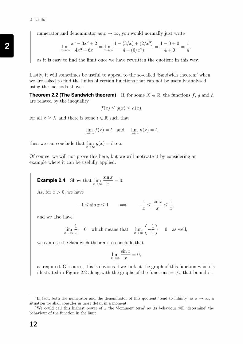
Lastly, it will sometimes be useful to appeal to the so-called ‘Sandwich theorem’ whenwe are asked to find the limits of certain functions that can not be usefully analysedusing the methods above.

Theorem 2.2 (The Sandwich theorem) If, for some X ∈ R, the functions f , g and hare related by the inequality

f(x) ≤ g(x) ≤ h(x),

for all x ≥ X and there is some l ∈ R such that

limx→∞

f(x) = l and limx→∞

h(x) = l,

then we can conclude that limx→∞

g(x) = l too.

Of course, we will not prove this here, but we will motivate it by considering anexample where it can be usefully applied.

Example 2.4 Show that limx→∞

sinx

x= 0.

As, for x > 0, we have

−1 ≤ sinx ≤ 1 =⇒ −1

x≤ sinx

x≤ 1

x,

and we also have

limx→∞

1

x= 0 which means that lim

x→∞

(−1

x

)= 0 as well,

we can use the Sandwich theorem to conclude that

limx→∞

sinx

x= 0,

as required. Of course, this is obvious if we look at the graph of this function which isillustrated in Figure 2.2 along with the graphs of the functions ±1/x that bound it.

4In fact, both the numerator and the denominator of this quotient ‘tend to infinity’ as x → ∞, asituation we shall consider in more detail in a moment.

5We could call this highest power of x the ‘dominant term’ as its behaviour will ‘determine’ thebehaviour of the function in the limit.

12

2

2.1. Limits

Figure 2.2: The dashed curve in the positive quadrant is the graph of the function 1/xand the dashed curve in the quadrant below this is the graph of the function −1/x. Thefunction sinx

x, whose graph is the solid line, always lies between these two curves for x > 0

and, because of this, we see that it must tend to zero as x→∞.

Activity 2.2 Find the following limits.

(a) limx→∞

x2 + x+ 1

x+ x2 + x3, (b) lim

x→∞(x+ sinx− 2)1/2

√x+ sinx− 2

.

Infinite limits

If f(x) is a function, we now want to ask what it means to say that this function tendsto infinity as x→∞, i.e. what it means to say that f(x)→∞ as x→∞ or, slightlyabusing our notation,6 that

limx→∞

f(x) =∞.

Intuitively, based on what we saw in 174 Calculus, we want to say that this means thatthe function, f(x), can take arbitrarily large values as we let x get larger and larger.But, more specifically, we mean that however large we want f(x) to be, let’s say wewant it to be larger than some real number, M , we can find a value of x, say X, forwhich f(x) is larger than M for all x ≥ X.7

6This is an abuse of our notation since, technically, what we denote by ‘∞’ is not a real number andso nothing can be equal to it. However, what we write here will be a very useful ‘notational convenience’.

7Technically, as you will see in 116 Abstract Mathematics, we say that f(x)→∞ as x→∞ if,

for any M > 0, there is an X such that, for all x ≥ X, f(x) ≥M .

13

2

2. Limits

We also want to consider functions, f(x), which tend to minus infinity as x→∞, i.e.where f(x)→ −∞ as x→∞ or, again slightly abusing our notation, where

limx→∞

f(x) = −∞.

Of course, we saw this kind of behaviour in 174 Calculus too and we want to say thatthis means that the function, f(x), can take negative values which are arbitrarily largein magnitude as we let x get larger and larger. But, it is perhaps easier to define this interms of what we have just seen, i.e. we say that

limx→∞

f(x) = −∞ if limx→∞

(− f(x)

)=∞,

i.e. if −f(x)→∞ as x→∞, then we must have f(x)→ −∞ as x→∞. Let’s nowconsider how we can actually find such limits.

Finding infinite limits

Again, as we saw above with finite limits, we can find infinite limits by considering somebasic functions that have infinite limits and then, by using some appropriate rules abouthow limits work, we can then find the limits of certain combinations of these basicfunctions. So, we start by stating some infinite limits that arise from basic functions, i.e.

(a) If f(x) = xb where b > 0 is a constant, then f(x)→∞ as x→∞.

(b) If f(x) = cx where c > 1 is a constant, then f(x)→∞ as x→∞.

(c) If f(x) = logd x where d > 1 is a constant, then f(x)→∞ as x→∞.

Then we have the rules which tell us how to find the limits of certain combinations ofthese basic functions which are stated in the following theorem.

Theorem 2.3 If f(x)→∞ as x→∞, then

(a) if c > 0 is a constant, then cf(x)→∞ as x→∞.

And, if we also have g(x)→∞ as x→∞, then

(b) f(x) + g(x)→∞ as x→∞.

(c) f(x)g(x)→∞ as x→∞.

Whereas, if we have g(x)→ m as x→∞ where m > 0 is a real number, then

(d) f(x) + g(x)→∞ as x→∞.

(e) f(x)g(x)→∞ as x→∞.

Here, the value of M > 0 tells us how large we want f(x) to be and, if we can show that there is anX such that f(x) ≥ M for all x ≥ X, then we have established that f(x) is always larger than M forthese values of x. Indeed, if we can do this for any value of M , we can guarantee that f(x) is getting‘arbitrarily large’ as x→∞. However, we will not make use of this formal definition here.

14

2

2.1. Limits

(f)f(x)

g(x)→∞ as x→∞.

We will not prove this theorem here even though some of the rules may be fairlyobvious, but it is important that you treat these rules with some care. In particular,although you can extend what we have seen in Theorem 2.3 fairly simply by doingActivity 2.3, there are some things that we won’t be able to do at the moment as you’llsee in Activity 2.4.

Activity 2.3 What is the analogue of Theorem 2.3(a) when c < 0 and what are theanalogues of Theorem 2.3(d)-(f) when m < 0?

Hence show that, if 0 < d < 1 is a constant, then logd x→ −∞ as x→∞.

Activity 2.4 What, if anything, can you say about the analogue of

(i) Theorem 2.3(a) when c = 0?

(ii) Theorem 2.3(b) and Theorem 2.3(c) when g(x)→ −∞ as x→∞?

(iii) Theorem 2.3(d)-(f) when m = 0?

Let’s now see how these results work by considering some examples.


(x3 + x+ 2).

Using Theorem 2.3(a) and what we saw before, we have

limx→∞

x3 =∞, limx→∞

x =∞ and limx→∞

2 = 2,

so, using Theorem 2.3(d), we have

limx→∞

(x+ 2) =∞,

so that, using Theorem 2.3(b), we get

limx→∞

(x3 + x+ 2) =∞,

as the answer.


x3 + 2x+ 2

x2 + 1.

We saw in Example 2.5 that the numerator of the function

x3 + 2x+ 2

x2 + 1,

tends to infinity as x→∞ and, using similar reasoning, the denominator tends toinfinity as x→∞ too. In particular, this means that we can’t use any of the results

15

2

2. Limits

in Theorem 2.3 on this function as it stands. However, if we divide the numeratorand the denominator of this function by the highest power of x in the denominator,8

i.e. x2, we getx3 + 2x+ 2

x2 + 1=x+ (2/x) + (2/x2)

1 + (1/x2),

and in this form the numerator still tends to infinity as x→∞, but the denominatornow tends to one which is a positive real number. Consequently, we can useTheorem 2.3(f) to see that

limx→∞

x3 + 2x+ 2

x2 + 1= lim

x→∞x+ (2/x) + (2/x2)

1 + (1/x2)=

limx→∞

[x+ (2/x) + (2/x2)

]1

=∞,

is the answer.


x+ 1√4x− 1

.

It should be clear that the numerator and the denominator of the function

x+ 1√4x− 1

,

both tend to infinity as x→∞ and so we are in a similar situation to the one inExample 2.6. So, as we did in that example, we divide the numerator and thedenominator of this function by the highest power of x in the denominator, i.e.

√x,

to getx+ 1√4x− 1

=

√x+ (1/

√x)√

4− (1/x),

and in this form the numerator still tends to infinity as x→∞, but the denominatornow tends to two — as we saw in Example 2.2 — which is a positive real number.Consequently, we can use Theorem 2.3(f) to see that

limx→∞

x+ 1√4x− 1

= limx→∞

√x+ (1/

√x)√

4− (1/x)=

limx→∞

[√x+ (1/

√x)]

2=∞,

is the answer.

Activity 2.5 Find the limits (a) limx→∞

(x2 − x3) and (b) limx→∞

x2 − sinx

x+ sinx.

8Of course, the highest power of x in the quotient is x3 (i.e. this is the ‘dominant term’), but if wedivide the numerator and denominator by this, we get

x3 + 2x+ 2

x2 + 1=

1 + (2/x2) + (2/x)

(1/x) + (1/x3).

And, this means that, as x→∞, the numerator tends to one and the denominator tends to zero, a casethat we can not deal with using Theorem 2.1(d). However, we will see in Example 2.8 that we can makesense of this once we have Theorem 2.4.

16

2

2.1. Limits

The relationship between infinite and finite limits

We have seen that, as x→∞, some functions have finite limits and others have infinitelimits but now we want to briefly discuss how these two types of limit are related. Thekey result here is the following theorem.

Theorem 2.4 (a) If f(x)→∞ as x→∞, then

limx→∞

1

f(x)= 0.

(b) If f(x)→ 0 as x→∞ and there is an M ∈ R such that

f(x) > 0 for all x > M , then limx→∞

1

f(x)=∞.

f(x) < 0 for all x > M , then limx→∞

1

f(x)= −∞.

Of course, the results in this theorem should be fairly obvious and we can see why if weconsider an example.

Example 2.8 Following on from Example 2.6, use Theorem 2.4 to verify that

limx→∞

x3 + 2x+ 2

x2 + 1=∞,

as we found there.9

The highest power of x in the quotient is x3,10 and if we divide the numerator anddenominator by this, we get

x3 + 2x+ 2

x2 + 1=

1 + (2/x2) + (2/x3)

(1/x) + (1/x3)=

(1 +

2

x2+

2

x3

)1

(1/x) + (1/x3).

Now, as x→∞, the first term in this product tends to one whereas, byTheorem 2.4, the second term tends to infinity as

1

x+

1

x3> 0,

for x > 0. Consequently, by Theorem 2.3, we see that

limx→∞

x3 + 2x+ 2

x2 + 1=∞,

as expected.

9This example follows on from the discussion in footnote 8.10That is, x3 is the ‘dominant term’ here.

17

2

2. Limits

Limits that don’t exist

If we have a function f(x) and we find that

limx→∞

f(x) = c,

where c is a real number or we find that f(x)→∞ (or −∞) as x→∞, we say that thelimit of f(x) as x→∞ exists. However, not every function has a limit as x→∞ and,in such cases, we say that this limit does not exist.

Example 2.9 Explain why limx→∞

sinx does not exist.

As we know from 174 Calculus, the function sin x, which is illustrated in Figure 2.3,oscillates between the values of 1 and −1 with a period of 2π. As such, this functionhas no limit as x→∞ since it never stays arbitrarily close to any value.

Figure 2.3: The graph of the function sin x for x ≥ 0.

However, although in this case the oscillations mean that a limit doesn’t exist, we sawin Example 2.4 that the function

sinx

x,

tends to zero as x→∞ even though it is oscillating.11 But, generally, some care mustbe taken when deciding whether an oscillating function has a limit as the next twoactivities illustrate.

11Of course, in this case it is the fact that the ‘amplitude’ of the oscillations decreases to zero as x→∞that guarantees that this limit is zero!

18

2

2.1. Limits

Activity 2.6 Consider the limits

(i) limx→∞

x(1 + sin x) and (ii) limx→∞

x(2 + sin x).

Do either of these limits exist? If the limit exists, what is it? (Hint: A sketch mayhelp!)

Activity 2.7 Consider the limits

(i) limx→∞

√sinx

xand (ii) lim

x→∞

√∣∣∣∣sinxx∣∣∣∣.

Do either of these limits exist? If the limit exists, what is it? (Hint: A sketch mayhelp!)

2.1.2 Limits at a point

Limits ‘at a point’ are concerned with the behaviour of a function, f(x), as x tends tosome finite value, say a, a situation we denoted by ‘x→ a’ in 174 Calculus. Indeed, aswe saw in that course, this kind of information is useful when we were sketching thegraph of a function because it told us what was happening as x gets ‘very close to a’,especially if the behaviour of the function as x tends to a from above (denoted byx→ a+) was different to its behaviour as x tends to a from below (denoted by x→ a−).In this section, we consider exactly what this kind of limit means and see how we canfind such a limit (if it exists) in some straightforward cases.

Finite limits

Suppose that l is a real number and that f(x) is a function that is defined for all valuesof x < a.12 We start by asking what it means to say that f(x)→ l as x→ a−, or ‘as xtends to a from below’, i.e. what it means to say that

limx→a−

f(x) = l.

Intuitively, we would want to say that this means that we can ensure that f(x) is asclose to l as we want by taking values of x that are less than a but close enough to a.But, more specifically, we mean that however close we would like f(x) to be to l, thereis some value of x, say X, for which f(x) is as close to l as we wanted if X < x < a.13

12That is the function needs to be defined for all values of x less than a, but it need not be defined atx = a.

13Technically, as you will see in 116 Abstract Mathematics, we say that f(x)→ l as x→ a− for somereal number, l, if

for any ε > 0, there is a δ > 0 such that, for all x ∈ (a− δ, a), |f(x)− l| < ε.

Here, the value of ε > 0 tells us how close we want to be and, if we can show that there is a δ > 0 suchthat |f(x) − l| < ε for all x in the interval (a − δ, a), then we have established that f(x) is as close tol as we wanted for these values of x below x = a. Indeed, if we can do this for any value of ε, we can

19

2

2. Limits

Of course, we can also ask what it means to say that f(x)→ l as x→ a+, or ‘as x tendsto a from above’, i.e. what it means to say that

limx→a+

f(x) = l,

and, intuitively, we would want to say that this means that we can ensure that f(x) is asclose to l as we want by taking values of x that are greater than a but close enough to a.But, more specifically, we mean that however close we would like f(x) to be to l, thereis some value of x, say X, for which f(x) is as close to l as we wanted if a < x < X.14

Indeed, if both of the limits

limx→a−

f(x) and limx→a+

f(x),

exist and, furthermore, they are the same, then we say that the limit

limx→a

f(x),

exists and is equal to this common value. However, having said that, unless we need toworry about the limits of f(x) as x→ a− and as x→ a+ individually,15 we will often beable to find the limit of f(x) as x→ a straightaway. Let’s now consider how we canactually do this.

Finding finite limits

Again, as we saw with limits at infinity in Section 2.1.1, we can find finite limits byconsidering some basic functions that have finite limits and then, by using someappropriate rules about how limits work, we can then find the limits of certaincombinations of these basic functions. So, we start by stating some finite limits thatarise from basic functions, i.e.

(a) If f(x) = xn where n ∈ N, then f(x)→ an as x→ a.

(b) If f(x) = cx where c > 0, then f(x)→ ca as x→ a.

Then we have the rules which tell us how to find the limits of certain combinations ofthese functions which are stated in the following theorem.

guarantee that f(x) is getting ‘arbitrarily close’ to l as x → a−. However, we will not make use of thisformal definition here.

14Technically, as you will see in 116 Abstract Mathematics, we say that f(x)→ l as x→ a+ for somereal number, l, if

for any ε > 0, there is a δ > 0 such that, for all x ∈ (a, a− δ), |f(x)− l| < ε.

Here, the value of ε > 0 tells us how close we want to be and, if we can show that there is a δ > 0 suchthat |f(x) − l| < ε for all x in the interval (a, a − δ), then we have established that f(x) is as close tol as we wanted for these values of x above x = a. Indeed, if we can do this for any value of ε, we canguarantee that f(x) is getting ‘arbitrarily close’ to l as x → a+. However, we will not make use of thisformal definition here.

15For instance, if it is possible that one of them doesn’t exist or, if both of them exist, it is possiblethat they aren’t equal.

20

2

2.1. Limits

Theorem 2.5 Theorem 2.1 holds if x→∞ is replaced by x→ a−, x→ a+ or x→ a.

Of course, the same caveats apply as the ones we saw after the statement ofTheorem 2.1.

Example 2.10 Find limx→3

(x+ 3) and limx→3

x2 − 9

x− 3.

As we should expect, for the first limit, we have

limx→3

(x+ 3) = 3 + 3 = 6,

as illustrated in Figure 2.4(a) whereas for the second limit we note that, as long asx 6= 3, we have

x2 − 9

x− 3=

(x− 3)(x+ 3)

x− 3= x+ 3,

even though this function is not actually defined at x = 3. So, as the limit as x→ 3only considers what the function is doing around x = 3,16 we see that

limx→3

x2 − 9

x− 3= lim

x→3(x+ 3) = 3 + 3 = 6,

as illustrated in Figure 2.4(b). In particular, we observe that this limit is 6 eventhough this function is undefined at x = 3 and, as such, the point (3, 6) is not partof the graph of this function.

y = x+ 3

x

y

O3

3

−3

6 y = x2−9x+3

x

y

O3

3

−3

6

(a) (b)

Figure 2.4: Graphs of the two functions from Example 2.10. (Note that a ‘•’ means thatthis point is actually part of the graph of the function whereas a ‘◦’ means that this pointis not actually part of the graph of the function.)

16That is, whether it is actually defined at x = 3 is irrelevant when we consider the limit as x→ 3.

21

2

2. Limits


x2

x− 3.

As we anticipate no problems as x→ 2, we use Theorem 2.2 to get

limx→2

x2 = 22 = 4 and limx→2

(x− 3) = 2− 3 = −1,

and, as the second of these limits is non-zero, Theorem 2.2(d) then gives us

limx→2

x2

x− 3=

4

−1= −4,

as the answer.

Note: As this is fairly obvious, once you have understood the results above, youwould normally just write

limx→2

x2

x− 3=

22

2− 3=

4

−1= −4,

having taken care to observe that we are not dividing by zero.


√1 + x− 1

x.

We start by noting that, in this case, we can not simply work out the limit of thisquotient by considering the limits of the numerator and the denominator as x→ 0because both of these limits are zero.

In cases such as this, we employ the useful ‘trick’, called rationalisation, ofmultiplying the numerator and the denominator by

√1 + x+ 1 as this gives us

√1 + x− 1

x=

(√

1 + x− 1)(√

1 + x+ 1)

x(√

1 + x+ 1)=

(1 + x)− 1

x(√

1 + x+ 1)=

1√1 + x+ 1

.

Having done this, we now see that the limits of the numerator and the denominatoras x→ 0 are both non-zero, and this gives us

limx→0

√1 + x− 1

x= lim

x→0

1√1 + x+ 1

=1√

1 + 0 + 1=

1

1 + 1=

1

2,

as the answer.


x2 − 3x+ 2

1− x2.

We start by noting that, in this case, we can not simply work out the limit of thisquotient by considering the limits of the numerator and the denominator as x→ 1because both of these limits are zero.

In cases such as this, where the numerator and the denominator are polynomials, the

22

2

2.1. Limits

fact that both of them are zero at x = 1 guarantees that they both have x− 1 as afactor. So, if we employ the useful ‘trick’ of factorising the numerator anddenominator, we see that we have

x2 − 3x+ 2

1− x2=

(x− 1)(x− 2)

(1− x)(1 + x)= −x− 2

1 + x,

as long as x 6= 1.17 So, as the limit x→ 1 only considers what the function is doingaround x = 1, we have

limx→1

x2 − 3x+ 2

1− x2= − lim

x→1

x− 2

1 + x= −1− 2

1 + 1=

1

2,

as the answer.

Infinite limits

If f(x) is a function, we now want to ask what it means to say that this function tendsto infinity as x→ a− or as x→ a+, i.e. what it means to say that f(x)→∞ as x→ a−

or as x→ a+ which, again abusing our notation, we would write as

limx→a−

f(x) =∞ or limx→a+

f(x) =∞.

Of course, intuitively, as we saw in 174 Calculus, we would want to say this means thatthe curve y = f(x) has a vertical asymptote given by x = a, i.e. a vertical line that thecurve gets arbitrarily close to. But, more specifically, when we say that

f(x)→∞ as x→ a− we mean that however large we want f(x) to be, let’s say wewant it to be larger than some real number, M , we can find a value of x, say X, forwhich f(x) is larger than M if X < x < a.18

f(x)→∞ as x→ a+ we mean that however large we want f(x) to be, let’s say wewant it to be larger than some real number, M , we can find a value of x, say X, forwhich f(x) is larger than M if a < x < X.19

17Of course, this function is not actually defined at x = 1.18Technically, as you will see in 116 Abstract Mathematics, we say that f(x)→∞ as x→ a−, if

for any M > 0, there is a δ > 0 such that, for all x ∈ (a− δ, a), f(x) > M .

Here, the value of M > 0 tells us how large we want f(x) to be and, if we can show that there is a δ > 0such that f(x) > M for all x in the interval (a−δ, a), then we have established that f(x) is always largerthan M for these values of x below x = a. Indeed, if we can do this for any value of M , we can guaranteethat f(x) is getting ‘arbitrarily large’ as x→ a−. However, we will not make use of this formal definitionhere.

19Technically, as you will see in 116 Abstract Mathematics, we say that f(x)→∞ as x→ a+, if

for any M > 0, there is a δ > 0 such that, for all x ∈ (a, a+ δ), f(x) > M .

Here, the value of M > 0 tells us how large we want f(x) to be and, if we can show that there is a δ > 0such that f(x) > M for all x in the interval (a, a+δ), then we have established that f(x) is always largerthan M for these values of x above x = a. Indeed, if we can do this for any value of M , we can guaranteethat f(x) is getting ‘arbitrarily large’ as x→ a+. However, we will not make use of this formal definitionhere.

23

2

2. Limits

And, if we find that

limx→a−

(− f(x)

)=∞ or lim

x→a+

(− f(x)

)=∞,

we say that f(x) tends to minus infinity as x→ a− or as x→ a+ respectively. That is,this is what it means to say that f(x)→ −∞ as x→ a− or as x→ a+ which, againabusing our notation, we could write as

limx→a−

f(x) = −∞ or limx→a+

f(x) = −∞,

respectively.

Finding infinite limits

Let’s start with a simple example.

Example 2.14 Find limx→0−

1

xand lim

x→0+

1

x.

For the first limit, we see that for values of x < 0, the function 1/x is negative andso −1/x is positive. Indeed, as these x < 0 get closer to zero, we find that −1/xtends to infinity, i.e.

limx→0−

(− 1

x

)=∞ =⇒ lim

x→0−

1

x= −∞.

For the second limit, we see that for values of x > 0, the function 1/x is positiveand, as these x > 0 get closer to zero, we find that 1/x tends to infinity, i.e.

limx→0+

1

x=∞.

Of course, as these two limits are not the same, this means that the limit

limx→0

1

x,

does not exist and, indeed, we can see that this function has a vertical asymptote atx = 0.

But, generally, as we saw above with finite limits, we can find infinite limits byconsidering some basic functions that have infinite limits and then, by using someappropriate rules about how limits work, we can find the limits of certain combinationsof these basic functions. So, we start by stating some infinite limits that arise from basicfunctions, i.e.

(a) If f(x) = xb where b < 0 is a constant, then f(x)→∞ as x→ 0+.

(b) If f(x) = logd x where d > 1 is a constant, then f(x)→ −∞ as x→ 0+.

However, as you will see in Activity 2.8, some care must be taken with the analogue of(a) when we are considering limits as x→ 0−.

24

2

2.1. Limits

Activity 2.8 Suppose that f(x) = xb where b < 0 is a constant. What can you sayabout the limit of this function as x→ 0− when (i) b = −1, (ii) b = −2 and (iii)b = −1/2?

Then, we have the rules which tell us how to find the limits of certain combinations ofthese basic functions which are stated in the following theorem.

Theorem 2.6 Theorem 2.3 holds if x→∞ is replaced by x→ a−, x→ a+ or x→ a.

Of course, the same caveats apply as the ones we saw after the statement ofTheorem 2.3. As an example of why these rules work, we can think of something similarto Example 2.13, which will no longer give us a finite limit.

Example 2.15 Find limx→1−

x2 − 3x+ 3

1− x2and lim

x→1+

x2 − 3x+ 3

1− x2.

We start by noting that, in this case, we can not simply work out the limit of thisquotient by considering the limits of the numerator and the denominator as x→ 1−

or as x→ 1+ because, in both cases, the limit of the denominator is zero.

In cases such as this, where the denominator is a polynomial, the fact that it is zeroat x = 1 guarantees that it has x− 1 as a factor. So, if we employ the useful ‘trick’of factorising the denominator, we see that we have

x2 − 3x+ 3

1− x2=

x2 − 3x+ 3

(1− x)(1 + x),

and, of course, this function is not actually defined at x = 1. So, as the limit x→ 1−

only considers what the function is doing below x = 1, we have

limx→1−

x2 − 3x+ 3

1− x2= lim

x→1−

x2 − 3x+ 3

(1− x)(1 + x).

Now, we can see that, without the 1− x term in the denominator, we have

limx→1−

x2 − 3x+ 3

1 + x=

12 − 3 + 3

2=

1

2,

and this is positive whereas 1− x itself tends to zero through positive values asx→ 1− since this gives values of x < 1. Consequently, as we are dividing a positivenumber, i.e. 1/2, by smaller and smaller positive numbers, we see that

limx→1−

x2 − 3x+ 3

1− x2= lim

x→1−

x2 − 3x+ 3

(1− x)(1 + x)=∞.

Then, applying similar reasoning, we see that as the limit x→ 1+ only considerswhat the function is doing above x = 1, we have

limx→1+

x2 − 3x+ 3

1− x2= lim

x→1+

x2 − 3x+ 3

(1− x)(1 + x).

25

2

2. Limits

So, we still have

limx→1+

x2 − 3x+ 3

1 + x=

12 − 3 + 3

2=

1

2,

and this is positive whereas 1− x itself now tends to zero through negative values asx→ 1+ since this gives values of x > 1. Consequently, as we are dividing a positivenumber, i.e. 1/2, by smaller and smaller [in magnitude] negative numbers, we seethat

limx→1+

x2 − 3x+ 3

1− x2= lim

x→1+

x2 − 3x+ 3

(1− x)(1 + x)= −∞.

Of course, as these two limits are not the same, this means that the limit

limx→1

x2 − 3x+ 3

1− x2,

does not exist and, indeed, we can see that this function has a vertical asymptote atx = 1.

The relationship between infinite and finite limits

We have seen that, as x→ a− or as x→ a+, some functions have finite limits andothers have infinite limits but now we want to briefly discuss how these two types oflimit are related. The key result here is the following theorem.

Theorem 2.7 (a) If f(x)→∞ as x→ a−, then

limx→a−

1

f(x)= 0,

and this result also holds if a− is replaced by a+.

(b) If f(x)→ 0 as x→ a− and there is a δ ∈ R such that

f(x) > 0 for all a− δ < x < a, then limx→∞

1

f(x)=∞.

f(x) < 0 for all a− δ < x < a, then limx→∞

1

f(x)= −∞.

The analogue of this result holds if a− is replaced by a+.

Of course, the results in this theorem should be fairly obvious and we have used themimplicitly in Example 2.15.

Limits that don’t exist

If we have a function f(x) and we find that

limx→a−

f(x) = c,

where c is a real number or we find that f(x)→∞ (or −∞) as x→ a−, we say that thelimit of f(x) as x→ a− exists. And, of course, we can say similar things in the limit as

26

2

2.1. Limits

x→ a+ or x→ a. However, not every function has a limit as x→ a− or x→ a+ orx→ a and, in such cases, we say that this limit does not exist.

Example 2.16 Consider the function

f(x) =

{x+ 3 if x ≤ 3

12− 3x if x > 3.

What can we say about the limit of this function as x→ 3?

Here we can see that we may have to worry about what is happening with thisfunction at x = 3 and so it makes sense to find its limits as x→ 3− and as x→ 3+.In particular, we see that as x→ 3−, we are concerned with values of x < 3 that aregetting closer to x = 3 and so we have

limx→3−

f(x) = limx→3−

(x+ 3) = 3 + 3 = 6,

whereas as x→ 3+, we are concerned with values of x > 3 that are getting closer tox = 3 and so we have

limx→3+

f(x) = limx→3+

(12− 3x) = 12− 3(3) = 3.

So, although both of these limits exist, they are not equal and so the limit of f(x) asx→ 3 does not exist.

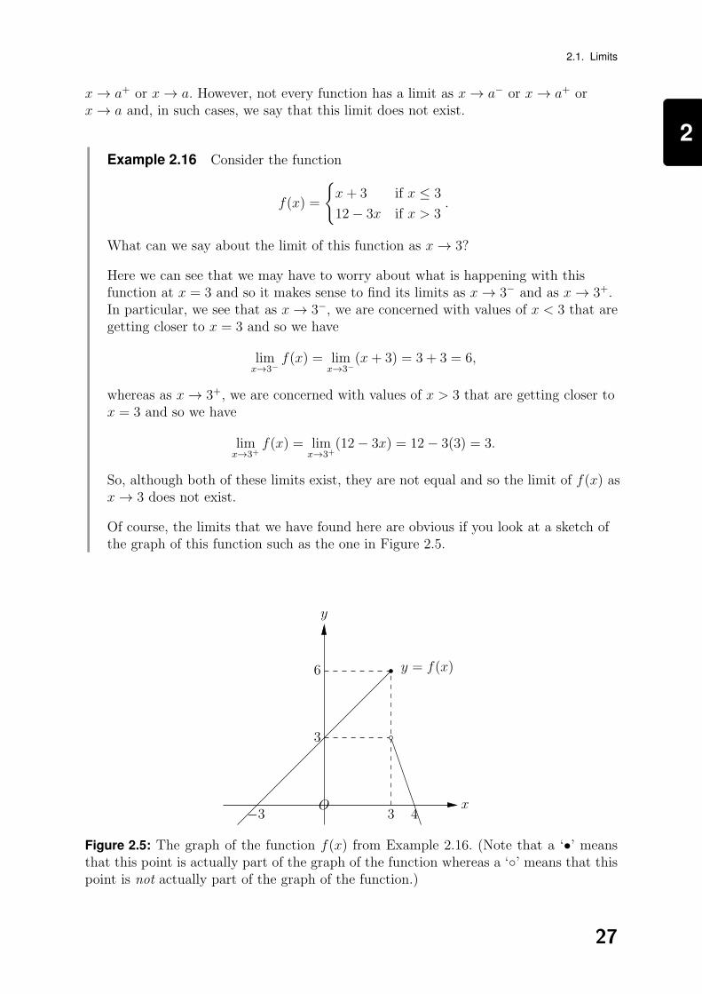
Of course, the limits that we have found here are obvious if you look at a sketch ofthe graph of this function such as the one in Figure 2.5.

y = f(x)

x

y

O3

3

−3

6

4

Figure 2.5: The graph of the function f(x) from Example 2.16. (Note that a ‘•’ meansthat this point is actually part of the graph of the function whereas a ‘◦’ means that thispoint is not actually part of the graph of the function.)

27

2

2. Limits

2.2 Some useful results that involve limits

2.2.1 Continuity

Intuitively, we say that a function is continuous at a point if it has no ‘breaks’ or‘jumps’ at that point and we can use limits to make this idea more precise. Inparticular, if a function, f(x), is such that both

limx→c

f(x) and f(c),

are defined and, furthermore, we have

limx→c

f(x) = f(c),

then we say that f(x) is continuous at x = c. Indeed, if the function is continuous atevery point in the interval (a, b), we say that it is continuous on that interval and if thefunction is continuous at every point in R, we simply say that it is continuous.

Some continuous functions

Most of the basic functions that we considered in 174 Calculus are continuous, inparticular, it should be clear that the following functions are all continuous over theirdomains.

Power functions f : R→ R where f(x) = xn for n ∈ N.

Exponential functions f : R→ (0,∞) where f(x) = ax for positive a 6= 1.

Trigonometric functions f : R→ [−1, 1] where f(x) = sinx or f(x) = cos x.

Logarithmic functions f : (0,∞)→ R where f(x) = loga(x) for positive a 6= 1.

If you are in any doubt about the continuity of any of these functions, you shouldconsider what we know about their graphs from 174 Calculus.

Some useful results

Having seen which of our basic functions are continuous, we can then see how continuityis preserved when we take combinations of these functions by using the followingtheorem.

Theorem 2.8 If the functions f(x) and g(x) are continuous at x = c, then so are thefunctions

kf(x) where k ∈ R;

f(x) + g(x);

f(x)g(x);

f(x)

g(x)as long as g(c) 6= 0.

28

2

2.2. Some useful results that involve limits

Moreover, if f(x) is continuous at x = c and g(x) is continuous at d = f(c),20 then thecomposition (g ◦ f)(x) = g(f(x)) is also continuous at x = c.

Lastly, suppose that f−1(x) is the inverse of a function f(x) which is strictly increasing(or decreasing) over some interval (a, b). If f(x) is continuous at x = c for somec ∈ (a, b), then f−1(x) is also continuous at x = f(c).

Let’s take a moment to see how this all works by considering an example.

Example 2.17 Explain why the functionsinx

xis continuous for all x 6= 0.

We know from above that the functions sin x and x are continuous for all x ∈ R andso, by Theorem 2.6, we see that the function

sinx

x,

is also continuous as long as x 6= 0. Indeed, it should be clear that this function isnot continuous at x = 0 since it is not even defined there.

Notice, however, that we can sometimes ‘repair’ failures in continuity by taking a littlemore care with the definition of a function as the next example shows.

Example 2.18 Following on from Example 2.17, consider the function f : R→ Rgiven by f(0) = 1 and

f(x) =sinx

x,

when x 6= 0. Show that this function is continuous for all x ∈ R.

[Hint: You may assume thatsinx

x→ 1 as x→ 0. (See Example 2.22.)]

We saw in Example 2.17 that f(x) is continuous for all x 6= 0 and, using the hint, wesee that

limx→0

f(x) = limx→0

sinx

x= 1 = f(0),

which means that f(x) is continuous at x = 0 too.

2.2.2 Differentiability

We saw in 174 Calculus if f(x) is a function, then its derivative, f ′(x), is the functiondefined by

f ′(x) = limh→0

f(x+ h)− f(x)

h,

and, if f ′(c) exists, we say that f(x) is differentiable at x = c. Indeed, if the function isdifferentiable at every point in the interval (a, b), we say that it is differentiable on thatinterval and if the function is differentiable at every point in R, we simply say that it is

20So that, in particular, d is in the range of f which is, in turn, taken to be in the domain of g.

29

2

2. Limits

differentiable. Of course, we explored derivatives and what they tell us about functionsin some detail in 174 Calculus and so we will settle for a simple example of how thisworks.

Example 2.19 Find the derivative of the function f(x) =√x for x > 0.

Using the definition of the derivative, we have

f ′(x) = limh→0

f(x+ h)− f(x)

h= lim

h→0

√x+ h−√x

h,

where we require that x > 0 so that√x is defined. Of course, we can evaluate this

using the rationalisation ‘trick’ that we saw in Example 2.12, i.e. we multiply thenumerator and the denominator of

√x+ h−√x

h,

by√x+ h+

√x to get

√x+ h−√x

h=

(√x+ h−√x

h

)(√x+ h+

√x√

x+ h+√x

)=

(x+ h)− xh(√x+ h+

√x)

=1√

x+ h+√x,

so that we have√x+ h−√x

h=

1√x+ h+

√x→ 1√

x+√x

=1

2√x,

as h→ 0. This then means that we have

f ′(x) = limh→0

f(x+ h)− f(x)

h= lim

h→0

√x+ h−√x

h=

1

2√x,

which is the answer we should have been expecting.

Activity 2.9 Using only the definition, find the derivative of the functionf(x) = x−1 for x 6= 0.

One useful thing to note is that ‘differentiability implies continuity’ in the followingsense.

Theorem 2.9 If the function, f(x), is differentiable at x = c, then it is continuous atx = c.

To see why this works, consider that if the function, f(x), is differentiable at x = c,then we know that f ′(c) exists and is given by

f ′(c) = limh→0

f(c+ h)− f(c)

h,

which means that if we consider the limit as h→ 0 of the function

f(c+ h)− f(c),

30

2


we can multiply the numerator and denominator by h to get

limh→0

(f(c+ h)− f(c)

)= lim

h→0h

(f(c+ h)− f(c)

h

)= (0)f ′(c) = 0.

But, this means thatlimh→0

f(c+ h) = f(c),

which establishes that f(x) is continuous at x = c.

However, the converse of this theorem is not true as the next activity shows.

Activity 2.10 Show that the function f(x) = |x| is continuous at x = 0, but that itis not differentiable at that point.

2.2.3 Taylor series and Taylor’s theorem

In 174 Calculus, we saw that the Taylor series for a function, f(x), around some pointx = c was given by

f(x) = f(c) + (x− c)f ′(c) +(x− c)2

2!f ′′(c) + · · ·+ (x− c)n

n!f (n)(c) + · · · ,

and, in the case where c = 0, we called this the Maclaurin series for f(x). Indeed, inthat course, we used such series to find approximations to the value of the function f(x)for values of x close to x = c. In particular, we defined the nth-order approximation tof(x) around the point x = c to be the polynomial, let’s call it Pn(x), given by

Pn(x) = f(c) + (x− c)f ′(c) +(x− c)2

2!f ′′(c) + · · ·+ (x− c)n

n!f (n)(c).

But, we now want to use a result, called Taylor’s theorem, which will allow us toinvestigate how accurate such approximations are.

Theorem 2.10 (Taylor’s theorem) If f(x) is a function defined on the interval (a, b)and all of its derivatives up to f (n+1)(x) exist on (a, b), then for any c, x ∈ (a, b) and anyn ∈ N, we have

f(x) = Pn(x) +(x− c)n+1

(n+ 1)!f (n+1)(d),

for some d lying [strictly] between c and x. In particular, we call

(x− c)n+1

(n+ 1)!f (n+1)(d),

the remainder term associated with Pn(x).

Notice that, in Taylor’s theorem, the remainder term tells you about the size of thedifference between f(x) and Pn(x), i.e. the size of the difference between what we aretrying to approximate and the approximation that we have found. As such, if we havereason to believe that the remainder term is small, then we can be assured that Pn(x) isa good approximation to f(x). Indeed, using Taylor’s theorem, we can actually findbounds that determine just how accurate our approximation is as the next exampleshows.

31

2

2. Limits

Example 2.20 Find the Taylor series for e−x about x = 0 and use it to find athird-order approximation to e−1. Then use Taylor’s theorem to find an upper boundon the difference between the true value of e−1 and this approximation to it.

If we take f(x) = e−x we have

f ′(x) = − e−x, f ′′(x) = e−x, f ′′′(x) = − e−x,

and, spotting the pattern, we see that f (n)(x) = (−1)n e−x for n ≥ 1. Thus, we havef(0) = 1 and f (n)(0) = (−1)n for n ≥ 1, which means that

e−x = 1 + (x− 0)(−1) +(x− 0)2

2!(1) +

(x− 0)3

3!(−1) + · · ·+ (x− 0)n

n!(−1)n + · · ·

= 1− x+x2

2!− x3

3!+ · · ·+ (−1)n

xn

n!+ · · · ,

is the Taylor series for e−x about x = 0. Indeed, using this, we can see that athird-order approximation to e−1 is given by

1− 1 +1

2!− 1

3!=

1

2− 1

6=

1

3,

i.e. our third-order approximation to e−1 is 0.3333 to 4dp.

Referring to Taylor’s theorem, we can then see that the remainder term in this caseis given by

(1− 0)4

4!e−d =

e−d

24,

for some d lying between c = 0 and x = 1. That is, using Taylor’s theorem, we havefound that

e−1 =1

3+

e−d

24,

for some d ∈ (0, 1). This means that the difference between the true value of e−1 andour third-order approximation to it is given by

e−1−1

3=

e−d

24<

1

24,

as d > 0 means that e−d < 1. Thus, the difference between the true value of e−1 andour approximation is at most 1/24 (or 0.0417 to 4dp) and so this is the requiredupper bound.

Incidentally, the true value of e−1 is 0.3679 to 4dp and so the difference between thetrue value of e−1 and our approximation is

e−1−1

3= 0.3679− 0.3333 = 0.0346,

and, as expected, this difference is less than the upper bound that we found for thisquantity.

32

2


If we extend this idea, we can see that Taylor’s theorem can also be used to find usefulbounds on functions as the next example illustrates.

Example 2.21 Use Taylor’s theorem to show that

1− x < e−x < 1− x+x2

2,

when x > 0.

As we’ll soon see, it makes sense to use the first-order Taylor series for e−x aroundx = 0 and the associated remainder term, i.e. using Taylor’s theorem and what wesaw at the beginning of Example 2.20, we have

e−x = 1− x+x2

2e−d,

for some d ∈ (0, x) where x > 0. Now, as d > 0, we have e−d < 1 and so we can write

e−x = 1− x+x2

2e−d < 1− x+

x2

2,

but, we also know that e−d > 0 for all d ∈ R, and so we can also write

e−x = 1− x+x2

2e−d > 1− x.

So, putting these two inequalities together, we get

1− x < e−x < 1− x+x2

2,

when x > 0, as required.

And, although we won’t dwell too much on it here, we can see that the values of x forwhich the Taylor series ‘works’ — an idea we encountered briefly in 174 Calculus — arethose values of x for which the remainder term tends to zero as n→∞. This is because,if we have a value of x for which the remainder term tends to zero as n→∞, then itshould be clear that Pn(x) tends to f(x) as n→∞. That is, the value of f(x) is thesame as the value of

limn→∞

Pn(x) = limn→∞

n∑i=0

(x− c)ii!

f (i)(c),

which is just what we get when we keep all of the terms in the Taylor series.

Using Taylor series to find limits

One particularly important application of Taylor series in this course is that they allowus to find certain limits. In particular, if we have the Taylor series of some function,f(x), about the point x = c, we can often use it to deduce the limit of expressions thatinvolve f(x) as x→ c simply because, as x gets closer to c, we would expect f(x) to

33

2

2. Limits

take values that get closer to the values that arise from its Taylor series. Let’s consideran example of how this works.

Example 2.22 Use the Taylor series for sinx about x = 0 to find limx→0

sinx

x.

We know that the Taylor series for sinx about x = 0 gives us

sinx = x− x3

3!+ · · · ,

and so, we have

sinx

x=x− x3

3!+ · · ·

x= 1− x2

3!+ · · · .

Now, as x→ 0, we see that the x2 term (and all the higher-order terms that we haveomitted) should tend to zero,21 leaving us with

limx→0

sinx

x= lim

x→0

(1− x2

3!+ · · ·

)= 1,

as the answer.

In particular, we observe that this method is especially useful when we are looking atlimits as x→ 0 because we know a lot about the Taylor series of our basic functionsabout x = 0 from Section 3.4 of 174 Calculus.

Activity 2.11 Use the appropriate Taylor series to find the following limits.

(a) limx→0

1− cosx

x2, (b) lim

x→0

ln(1 + x)

x.

We now consider another important method for working out certain limits and, as weshall see, this also implicitly relies on the use of Taylor series.

2.2.4 L’Hôpital’s rule

Following on from our earlier discussion of limits, we know that there are still certaincases which we can not deal with. For instance, suppose that we have to find the limit

limx→a+

f(x)

g(x),

in the case where f(x) and g(x) both tend to zero as x→ a+. In such cases, we can’tuse Theorem 2.5 because g(x)→ 0 as x→ a+ but, as long as the stated conditions hold,we can use L’Hopital’s rule which runs as follows.

21If necessary, we can make this idea precise by using the appropriate remainder term, but we willgenerally be content with the more ‘intuitive’ calculation that we have presented here.

34

2


Theorem 2.11 (L’Hôpital’s rule: first form) Suppose that the functions f and g aredifferentiable on the interval (a, b) and that g′(x) 6= 0 for x ∈ (a, b). If

both limx→a+

f(x) = 0 and limx→a+

g(x) = 0, and

limx→a+

f ′(x)

g′(x)= L where L is a real number or ∞ or −∞,22

then

limx→a+

f(x)

g(x)= L,

too. Indeed, analogues of this rule hold when limx→a+

is replaced by

limx→b−

or limx→c

,

for some c ∈ (a, b) as well as when we have a is −∞ or b is ∞.

We won’t prove this rule here, but we can see why it works by using Taylor’s theorem.For instance, looking at f(x) about x = a, Taylor’s theorem dictates that

f(x) = f(a) + (x− a)f ′(d1)

for some d1 ∈ (a, x) as we are interested in x ∈ (a, b), whereas looking at g(x) aboutx = a, Taylor’s theorem dictates that

g(x) = g(a) + (x− a)g′(d2),

for some d2 ∈ (a, x) as, again, we are interested in x ∈ (a, b). This means that, lookingat our quotient, we have

f(x)

g(x)=f(a) + (x− a)f ′(d1)

g(a) + (x− a)g′(d2).

But, we are given that

limx→a+

f(x) = 0 and limx→a+

g(x) = 0,

and so we have f(a) = 0 and g(a) = 0,23 which means that our quotient becomes

f(x)

g(x)=

(x− a)f ′(d1)

(x− a)g′(d2)=f ′(d1)

g′(d2),

as we can assume that x 6= a if we are taking the limit as x→ a+. Thus, we have

limx→a+

f(x)

g(x)= lim

x→a+f ′(d1)

g′(d2)= lim

x→a+f ′(x)

g′(x),

provided that, as assumed in Theorem 2.11, this last limit exists.24

22That is, this limit exists.23Observe that, using Theorem 2.9, the fact that f and g are differentiable on (a, b) implies that they

must be continuous on (a, b) as well.24Observe that the last equality arises because, if d1 and d2 are in the interval (a, x), we can see that

they must both tend to a from above when x→ a+.

35

2

2. Limits

Activity 2.12 Given that f(x) and g(x) are differentiable functions which bothtend to zero as x→∞, use the substitution x = 1/t and Theorem 2.11 to show that

limx→∞

f(x)

g(x)= lim

x→∞f ′(x)

g′(x),

provided that the limit on the right-hand side exists.

Let’s now look at some examples of how L’Hopital’s rule can be applied.

Example 2.23 Use L’Hopital’s rule to find limx→0

1− cosx

xand lim

x→0

ln(1 + x)

x.

For the first limit, we note that the numerator and the denominator both tend tozero as x→ 0 and we also have

f(x)

g(x)=

1− cosx

x=⇒ f ′(x)

g′(x)=

sinx

1,

where, as x→ 0, the limit of this second quotient is zero. So, using L’Hopital’s rule,we have

limx→0

1− cosx

x= lim

x→0

sinx

1= 0,

as the answer.

For the second limit, we again note that the numerator and the denominator bothtend to zero as x→ 0 and we also have

f(x)

g(x)=

ln(1 + x)

x=⇒ f ′(x)

g′(x)=

1/(1 + x)

1,

where, as x→ 0, the limit of this second quotient is one. So, using L’Hopital’s rule,we have

limx→0

ln(1 + x)

x= lim

x→0

1/(1 + x)

1= 1,

as the answer in agreement with what we saw in Activity 2.11(b)

Activity 2.13 Following on from Example 2.22, use L’Hopital’s rule to verify that

limx→0

sinx

x= 1.

Another case where we run into problems involves the limit

limx→a+

f(x)

g(x),

in the case where f(x) and g(x) both tend to infinity as x→ a+. In such cases, we can’tuse Theorem 2.7 because this case isn’t covered but, as long as the stated conditionshold, we can use another form of L’Hopital’s rule which runs as follows.

36

2


Theorem 2.12 (L’Hôpital’s rule: second form) Suppose that the functions f and gare differentiable on the interval (a, b) and that g′(x) 6= 0 for x ∈ (a, b). If

both

∣∣∣∣ limx→a+

f(x)

∣∣∣∣ =∞ and

∣∣∣∣ limx→a+

g(x)

∣∣∣∣ =∞, and

limx→a+

f ′(x)

g′(x)= L where L is a real number or ∞ or −∞,25

then

limx→a+

f(x)

g(x)= L,

too. Indeed, analogues of this rule hold when limx→a+

is replaced by

limx→b−

or limx→c

,

where c ∈ (a, b) as well as when we have a is −∞ or b is ∞.

To get a sense of why this works observe that, if the limits of f(x) and g(x) are bothinfinity as x→ a+, we can see that 1/f(x) and 1/g(x) both tend to zero as x→ a+ andso, using Theorem 2.11, we have

limx→a+

f(x)

g(x)= lim

x→a+1/g(x)

1/f(x)= lim

x→a+g′(x)/[g(x)]2

f ′(x)/[f(x)]2=

(limx→a+

f(x)

g(x)

)2(limx→a+

g′(x)

f ′(x)

),

assuming that these limits exist. Then, if we also have (for the sake of argument) someL 6= 0 such that

limx→a+

f ′(x)

g′(x)= L,

we see that this gives us

limx→a+

f(x)

g(x)= L,

too. Of course, this isn’t a proof of Theorem 2.12, but it does indicate how it is relatedto Theorem 2.11 if we aren’t being that careful. Let’s look at an example of how it canbe applied.

Example 2.24 Use L’Hopital’s rule to find limx→∞

ln(1 + x)

x.

We note that the numerator and the denominator both tend to infinity as x→∞and we also have

f(x)

g(x)=

ln(1 + x)

x=⇒ f ′(x)

g′(x)=

1/(1 + x)

1,

where, as x→∞, the limit of this second quotient is zero. So, using L’Hopital’s rule,we have

limx→∞

ln(1 + x)

x= lim

x→∞1/(1 + x)

1= 0,

as the answer.

25That is, this limit exists.

37

2

2. Limits

Activity 2.14 Use L’Hopital’s rule to find limx→∞

x(π

2− tan−1 x

).

Lastly, as you will see in the next activity, some care must be taken when finding limitswith L’Hopital’s rule as it is not always applicable.

Activity 2.15 Find the limits

(a) limx→0+

lnx

xand (b) lim

x→∞x+ sin x

x.

Why is L’Hopital’s rule not applicable for either of these limits?

Learning outcomes

At the end of this chapter and having completed the relevant reading and activities, youshould be able to:

find limits or explain why they don’t exist;

assess whether a function is continuous;

find derivatives using the definition of the derivative;

use Taylor series to find limits and Taylor’s theorem to find bounds;

use L’Hopital’s rule to find limits.

Solutions to activities

Solution to activity 2.1

We are given that f(x)→ l and g(x)→ m as x→∞ where l,m ∈ R, and so usingTheorem 2.1(a) with c = −1 and (b), we see that

f(x)− g(x) = f(x) + [−g(x)]→ l + [−m] = l −m as x→∞,

and, for any constants c and d, we also have

cf(x) + dg(x) = [cf(x)] + [dg(x)]→ cl + dm as x→∞,

again using Theorem 2.1(a) and (b).


For (a), we follow the method in Example 2.3 and divide the numerator anddenominator by the highest power of x that occurs in the given quotient. In this case,the highest power of x in the quotient is x3 and so we get

limx→∞

x2 + x+ 1

x+ x2 + x3= lim

x→∞(1/x) + (1/x2) + (1/x3)

(1/x2) + (1/x) + 1=

0 + 0 + 0

0 + 0 + 1=

0

1= 0.

38

2

2.2. Solutions to activities

For (b), we note that the highest power of x in the quotient is x1/2 and so, using thesame method as in (a), we get

limx→∞

(x+ sinx− 2)1/2

√x+ sinx− 2

= limx→∞

(1 + sinx

x− 2

x

)1/2

1 + sinx√x− 2√

x

.

Now, from Example 2.4, we know that

limx→∞

sinx

x= 0,

and so, as x→∞, the numerator has a limit given by (1 + 0 + 0)1/2 = 1 if we useTheorem 2.1(e). Further, in the denominator, we see that

limx→∞

sinx√x

= 0,

if, following Example 2.4, we use the Sandwich theorem with the inequality

− 1√x≤ sinx√

x≤ 1√

x,

which clearly holds for x > 0. So, overall, we have

limx→∞

(x+ sinx− 2)1/2

√x+ sinx− 2

= limx→∞

(1 + sinx

x− 2

x

)1/2

1 + sinx√x− 2√

x

=1

1 + 0 + 0= 1,

as our final answer.


Given that f(x)→∞ as x→∞, we see that the analogue of Theorem 2.3(a) whenc < 0 is

cf(x)→ −∞ as x→∞,whereas, given that g(x)→ m as x→∞ where m < 0 is a real number, we see that theanalogues of Theorem 2.3(d)-(f) are

f(x) + g(x)→∞, f(x)g(x)→ −∞ andf(x)

g(x)→ −∞,

as x→∞.

We also see that, if 0 < d < 1, we have (say) ln d < 0 and lnx→∞ as x→∞ so, usingthe ‘change of base formula’ for logarithms, we have

logd x =lnx

ln d→ −∞,

as x→∞ using our analogue of Theorem 2.3(a) from above.

39

2

2. Limits


For (i), we consider the analogue of Theorem 2.3(a) and note that regardless of the factthat f(x)→∞ as x→∞, if we take c = 0, we have

cf(x) = 0→ 0 as x→∞.

For (ii), we see that if f(x)→∞ and g(x)→ −∞ as x→∞, then the analogue ofTheorem 2.3(b) tells us nothing since we can make no sense of ‘∞−∞’. But, theanalogue of Theorem 2.3(c) is

f(x)g(x)→ −∞ as x→∞,

as the result of the product will be negative and arbitrarily large in magnitude.

For (iii), we see that if f(x)→∞ and g(x)→ 0 as x→∞, then the analogue ofTheorem 2.3(d) is

f(x) + g(x)→∞ as x→∞,but the analogue of Theorem 2.3(e) tells us nothing since we can make no sense of‘∞· 0’. The analogue of Theorem 2.3(f) also tells us nothing in this case as we can makeno sense of ‘∞/0’.26


For (a), notice that, as it stands, we can make no sense of x2 − x3 as x→∞ because wecan make no sense of ‘∞−∞’. However, if we consider that the highest power of x hereis x3 (i.e. this is the ‘dominant term’), we see that using the analogue of Theorem 2.3(e)that we saw in Activity 2.3, we have

limx→∞

(x2 − x3) = limx→∞

x3

(1

x− 1

)= −∞,

since, as x→∞, the first term in the product tends to ∞ whereas the second termterm tends to −1.

For (b), following on from what we saw in Example 2.6, we see that dividing thenumerator and denominator by the highest power of x in the denominator, i.e. x, we get

limx→∞

x2 − sinx

x+ sinx= lim

x→∞

x− sinxx

1 + sinxx

=

limx→∞

(x− sinx

x

)1

=∞,

if we use Theorem 2.3(f) and the result from Example 2.4.

26However, as we will see in Theorem 2.4, we can make some sense of this if we have some informationabout the sign of g(x).

40

2



For (i), let’s consider the function

f(x) = x(1 + sin x),

for x ≥ 0 so that, since −1 ≤ sinx ≤ 1, we have

0 ≤ 1 + sin x ≤ 2 =⇒ 0 ≤ x(1 + sin x) ≤ 2x =⇒ 0 ≤ f(x) ≤ 2x,

and so the graph of the curve y = f(x) is always between the straight lines y = 0 (i.e.the x-axis) and y = 2x. In particular, given the sin x term in f(x), we would expect thiscurve to ‘oscillate’ between these two straight lines. Consequently, we should anticipatethat a rough sketch of this curve would look something like the one in Figure 2.6(a).Indeed, with this sketch, it should be clear that the limit

limx→∞

x(1 + sin x),

does not exist since, as x→∞, f(x) neither stays arbitrarily close to any finite value(i.e. there is clearly no finite limit) nor is it always getting arbitrarily large (i.e. itclearly doesn’t tend to infinity).

For (ii), let’s consider the function

g(x) = x(2 + sin x),

for x ≥ 0 so that, since −1 ≤ sinx ≤ 1, we have

1 ≤ 2 + sin x ≤ 3 =⇒ x ≤ x(2 + sin x) ≤ 3x =⇒ x ≤ g(x) ≤ 3x,

and so the graph of the curve y = g(x) is always between the straight lines y = x andy = 3x. In particular, given the sin x term in g(x), we would expect this curve to‘oscillate’ between these two straight lines. Consequently, we should anticipate that arough sketch of this curve would look something like the one in Figure 2.6(b). Indeed,with this sketch, it should be clear that we have

limx→∞

x(2 + sin x) =∞,

as, for x ≥ 0, g(x) ≥ x and so g(x) must tend to infinity as x→∞.


For (i), we see that the limit

limx→∞

√sinx

x,

does not exist because, although

limx→∞

sinx

x= 0,

as we saw in Example 2.4, we cannot take the limit of√sinx

x,

41

2

2. Limits

(a) (b)

Figure 2.6: The sketches for Activity 2.6. (a) The dashed line is y = 2x and the solidcurve that ‘oscillates’ between this line and the x-axis (i.e. the line y = 0) is y = f(x).(b) The dotted line is y = x, the dashed line is y = 3x and the solid curve that ‘oscillates’between these two lines is y = g(x).

as x→∞ because this is not a well-defined function from R to R. In particular, we seethat if we want to consider its values (and whether they are staying arbitrarily close tosome limiting number — like, say, zero) for suitably large values of x, we find that forsome of those values of x, sin x will be negative and so the square root will not return avalue (i.e. a real number) for comparison.27 See, for instance, the rough sketch inFigure 2.7(a).

For (ii), we see that the function

f(x) =

√∣∣∣∣sinxx∣∣∣∣,

is well-defined for all x > 0 and so, unlike with (i), we can begin to make sense of thelimit of f(x) as x→∞. Indeed, since 0 ≤ | sinx| ≤ 1 for all x > 0, we can see that

0 ≤ f(x) ≤ 1√x,

and so, as 1/√x→ 0 as x→∞, we can conclude

limx→∞

√∣∣∣∣sinxx∣∣∣∣ = 0,

27Notice, in particular, that this is a case where Theorem 2.1(e) fails because with b = 1/2 and

l = limx→∞

f(x) = limx→∞

sinx

x= 0,

we can not make sense of

limx→∞

[f(x)]b,

even though lb = 01/2 = 0. This is why we insist that l > 0 in the statement of the theorem. (Becausel > 0 guarantees that f(x) > 0 for suitably large values of x and so we can meaningfully find thecorresponding values of, say, [f(x)]1/2.)

42

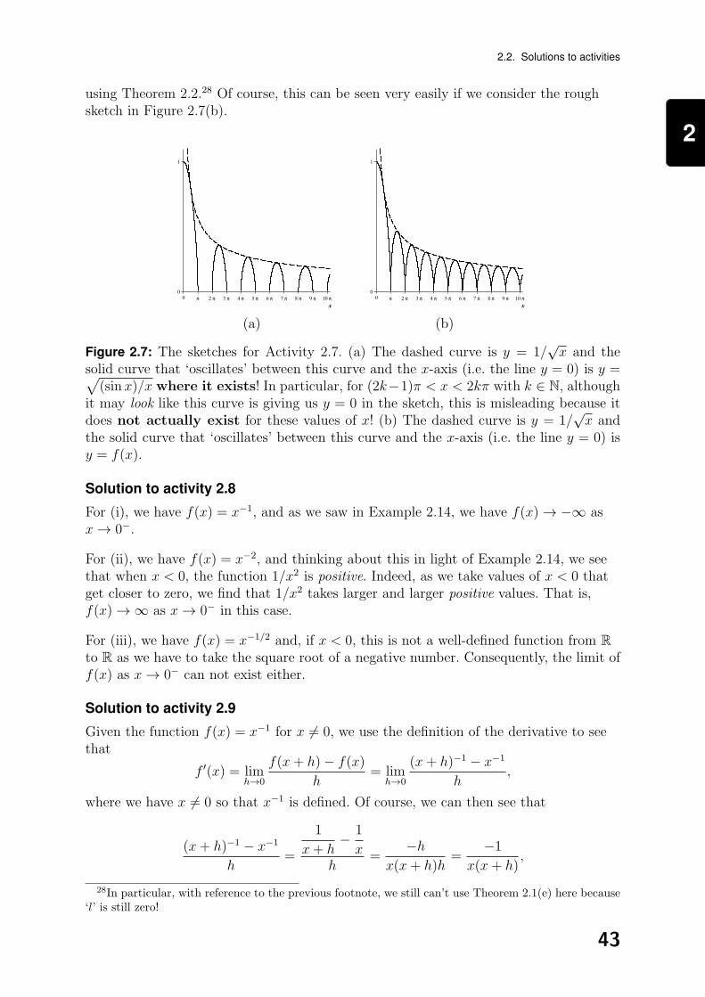
2


using Theorem 2.2.28 Of course, this can be seen very easily if we consider the roughsketch in Figure 2.7(b).

(a) (b)

Figure 2.7: The sketches for Activity 2.7. (a) The dashed curve is y = 1/√x and the

solid curve that ‘oscillates’ between this curve and the x-axis (i.e. the line y = 0) is y =√(sinx)/x where it exists! In particular, for (2k−1)π < x < 2kπ with k ∈ N, although

it may look like this curve is giving us y = 0 in the sketch, this is misleading because itdoes not actually exist for these values of x! (b) The dashed curve is y = 1/

√x and

the solid curve that ‘oscillates’ between this curve and the x-axis (i.e. the line y = 0) isy = f(x).


For (i), we have f(x) = x−1, and as we saw in Example 2.14, we have f(x)→ −∞ asx→ 0−.

For (ii), we have f(x) = x−2, and thinking about this in light of Example 2.14, we seethat when x < 0, the function 1/x2 is positive. Indeed, as we take values of x < 0 thatget closer to zero, we find that 1/x2 takes larger and larger positive values. That is,f(x)→∞ as x→ 0− in this case.

For (iii), we have f(x) = x−1/2 and, if x < 0, this is not a well-defined function from Rto R as we have to take the square root of a negative number. Consequently, the limit off(x) as x→ 0− can not exist either.


Given the function f(x) = x−1 for x 6= 0, we use the definition of the derivative to seethat

f ′(x) = limh→0

f(x+ h)− f(x)

h= lim

h→0

(x+ h)−1 − x−1

h,

where we have x 6= 0 so that x−1 is defined. Of course, we can then see that

(x+ h)−1 − x−1

h=

1

x+ h− 1

xh

=−h

x(x+ h)h=

−1

x(x+ h),

28In particular, with reference to the previous footnote, we still can’t use Theorem 2.1(e) here because‘l’ is still zero!

43

2

2. Limits

as we have h 6= 0 when we are considering the limit as h→ 0. This then means that wehave

f ′(x) = limh→0

−1

x(x+ h)= − 1

x2,

which is the answer we should have been expecting.


We see that the function f(x) = |x| is continuous at x = 0 because

limx→0

f(x) = limx→0|x| = |0| = 0 = f(0).

However, if we consider the definition of the derivative at x = 0, we need to look at

f(0 + h)− f(0)

h=|h| − 0

h=|h|h,

so that, when h < 0, we have |h| = −h and

limh→0−

f(0 + h)− f(0)

h= lim

h→0−

|h|h

= limh→0−

−hh

= limh→0−

(−1) = −1,

whereas, when h > 0, we have |h| = h and

limh→0+

f(0 + h)− f(0)

h= lim

h→0+

|h|h

= limh→0+

h

h= lim

h→0+1 = 1.

Consequently, we see that f(x) is not differentiable at x = 0 because

f ′(0) = limh→0

f(0 + h)− f(0)

h,

does not exist since the limits as h→ 0− and as h→ 0+ are not equal.


For (a), we know that the Taylor series for cos x about x = 0 gives us

cosx = 1− x2

2!+x4

4!− · · · ,

and so, we have

1− cosx

x2=

1−(

1− x2

2!+x4

4!− · · ·

)x2

=1

2!− x2

4!+ · · · .

Now, as x→ 0, we see that the x2 term (and all the higher-order terms that we haveomitted) should tend to zero, leaving us with

limx→0

1− cosx

x2= lim

x→0

(1

2!− x2

4!+ · · ·

)=

1

2,

as the answer.

44

2


For (b), we know that the Taylor series for ln(1 + x) about x = 0 gives us

ln(1 + x) = x− x2

2+ · · · ,

and so, we have

ln(1 + x)

x=x− x2

2+ · · ·

x= 1− x

2+ · · · .

Now, as x→ 0, we see that the x term (and all the higher-order terms that we haveomitted) should tend to zero, leaving us with

limx→0

ln(1 + x)

x= lim

x→0

(1− x

2+ · · ·

)= 1,

as the answer.


Essentially, the substitution x = 1/t gives us t→ 0+ as x→∞ and

limx→∞

f(x)

g(x)= lim

t→0+

f(1/t)

g(1/t),

where, as f(x) and g(x) both tend to zero as x→∞, we see that the functions f(1/t)and g(1/t) must also both tend to zero as t→ 0+. So, using the chain rule,Theorem 2.11 gives us

limt→0+

f(1/t)

g(1/t)= lim

t→0+

f ′(1/t)(−1/t2)

g′(1/t)(−1/t2)= lim

t→0+

f ′(1/t)

g′(1/t)= lim

x→∞f ′(x)

g′(x),

if we use the substitution x = 1/t again. So, putting this all together, we have shownthat

limx→∞

f(x)

g(x)= lim

x→∞f ′(x)

g′(x),

provided that the limit on the right-hand side exists.


To find the given limit, we note that the numerator and the denominator both tend tozero as x→ 0 and we also have

f(x)

g(x)=

sinx

x=⇒ f ′(x)

g′(x)=

cosx

1,

where, as x→ 0, the limit of this second quotient is one. So, using L’Hopital’s rule, wehave

limx→0

sinx

x= lim

x→0

cosx

1= 1,

as the answer in agreement with what we saw in Example 2.22.

45

2

2. Limits


In order to use L’Hopital’s rule to find the given limit, we first need to write the givenproduct as a quotient. Of course, the sensible way to do this is to write it as

limx→∞

x(π

2− tan−1 x

)= lim

x→∞

π2− tan−1 x

1/x,

so that we now have a quotient where the numerator and the denominator both tend tozero as x→∞. We also have

f(x)

g(x)=

π2− tan−1 x

1/x=⇒ f ′(x)

g′(x)=−1/(1 + x2)

−1/x2=

x2

1 + x2=

11x2

+ 1,

where, as x→∞, the limit of this second quotient is one. So, using L’Hopital’s rule, wehave

limx→∞

x(π

2− tan−1 x

)= lim

x→∞

π2− tan−1 x

1/x= lim

x→∞−1/(1 + x2)

−1/x2= lim

x→∞x2

1 + x2= 1,

as the answer.


For (a), L’Hopital’s rule is not applicable because, even though we have a quotient, thenumerator tends to minus infinity as x→ 0+ whereas the denominator tends to zero asx→ 0+. However, we can see that

limx→0+

lnx

x= lim

x→0+

(1

x

)lnx = −∞,

using the analogue of Theorem 2.3(c) that we saw in Activity 2.4(ii).

For (b), we see that L’Hopital’s rule is not applicable because, even though we have aquotient where the numerator and denominator both tend to infinity as x→∞, we findthat

f(x)

g(x)=x+ sin x

x=⇒ f ′(x)

g′(x)=

1 + cos x

1,

and, as x→∞, the limit of this second quotient does not exist. However, we can seethat

limx→∞

x+ sin x

x= lim

x→∞

(1 +

sinx

x

)= 1 + 0 = 1,

if we use the result from Example 2.4.

Exercises

Exercise 2.1

Find functions f and g which are such that, as x→∞, f(x)→∞ and g(x)→ 0 but

(a) f(x)g(x)→∞,

46

2

2.2. Solutions to exercises

(b) f(x)g(x)→ 0,

(c) f(x)g(x)→ −2,

(d) the limit of f(x)g(x) does not exist.

Exercise 2.2

Evaluate the following limits.

(a) limx→∞

[(x2 + x)1/2 − x

], (b) lim

x→∞

[(x3 + x2)1/3 − x

].

Exercise 2.3

Use L’Hopital’s rule to determine the following limits.

(a) limx→π/2

ln(1− cosx)

cosx, (b) lim

x→π/2(1− cosx)tanx.

Exercise 2.4

Using only the definition, find the derivative of the function f(x) = lnx for x > 0.

Exercise 2.5

For x 6= 0, consider the function

f(x) =1− cos(2x)

2x2.

Find the limit of f(x) as x→ 0 and hence define a function g(x) that is continuous forall x ∈ R which is the same as f(x) for all x 6= 0. Hence use the definition of thederivative to find g′(0).

Solutions to exercises

Solution to exercise 2.1

We can easily see that if we pick the functions f and g as follows they will satisfy therequirement that, as x→∞, f(x)→∞ and g(x)→ 0, as well as the additionalrequirement stated in the question.

(a) f(x) = x2 and g(x) =1

xgives us f(x)g(x) = x→∞ as x→∞.

(b) f(x) = x and g(x) =1

x2gives us f(x)g(x) =

1

x→ 0 as x→∞.

(c) f(x) = x and g(x) = −2

xgives us f(x)g(x) = −2→ −2 as x→∞.

47

2

2. Limits

(d) f(x) = x and g(x) =sinx

xgives us f(x)g(x) = sinx.

Of course, in (d), the limit of f(x)g(x) does not exist as x→∞.

The lesson here is that, as we observed in Activity 2.4(iii), if we only know thatf(x)→∞ and g(x)→ 0 as x→∞, we can infer nothing about the limit of f(x)g(x) asx→∞.


For (a), we can use the rationalisation ‘trick’ from Example 2.12 to see that

(x2 + x)1/2 − x =[(x2 + x)1/2 − x][(x2 + x)1/2 + x]

(x2 + x)1/2 + x=

(x2 + x)− x2

(x2 + x)1/2 + x=

x

(x2 + x)1/2 + x.

We then observe that, as in Example 2.3, we can divide the numerator and thedenominator by the highest power of x that occurs in the quotient, i.e. x itself, to get

x

(x2 + x)1/2 + x=

1(1 + 1

x

)1/2+ 1→ 1

1 + 1=

1

2,

as x→∞. That is, we have shown that

limx→∞

[(x2 + x)1/2 − x

]=

1

2.

For (b), we can also rationalise29 to get

(x3 + x2)1/3 − x =[(x3 + x2)1/3 − x][(x3 + x2)2/3 + x(x3 + x2)1/3 + x2]

(x3 + x2)2/3 + x(x3 + x2)1/3 + x2

=(x3 + x2)− x3

(x3 + x2)2/3 + x(x3 + x2)1/3 + x2

=x2

(x3 + x2)2/3 + x(x3 + x2)1/3 + x2.

We can then divide the numerator and the denominator by the highest power of x thatoccurs in the quotient, i.e. x2, to get

x2

(x3 + x2)2/3 + x(x3 + x2)1/3 + x2=

1(1 + 1

x

)2/3+(1 + 1

x

)1/3+ 1→ 1

1 + 1 + 1=

1

3,

29The rationalisation ‘trick’ in (a) takes ‘a− b’ and uses the well-known difference of two squares, i.e.

(a− b)(a+ b) = a2 − b2,

to ‘remove’ the square root. In (b), the rationalisation ‘trick’ also takes ‘a − b’ but we need to use theless well-known difference of two cubes, i.e.

(a− b)(a2 + ab+ b2) = a3 − b3,

to ‘remove’ the cube root.

48

2


as x→∞. That is, we have shown that

limx→∞

[(x3 + x2)1/3 − x

]=

1

3.

Incidentally, notice that, if we take n ∈ N we can consider the function

(xn + xn−1)1/n − x = x

[(1 +

1

x

)1/n

− 1

],

which replicates what we had in (a) and (b) if we take n = 2 and n = 3 respectively.Now, for suitably large x, 1/x is close to zero and so we can use the binomial theorem30

to see that (1 +

1

x

)1/n

= 1 +1

nx+

1n( 1n− 1)

2!x2+ · · · ,

which means that

(xn + xn−1)1/n − x = x

[(1 +

1

nx+

1n( 1n− 1)

2!x2+ · · ·

)− 1

]=

1

n+

1n( 1n− 1)

2!x+ · · · .

Consequently, as x→∞, we find that the term in 1/x (and all of the neglected terms)tend to zero, leaving us with

limx→∞

[(x2 + x)1/n − x

]=

1

n,

in agreement with what we saw above.


For (a), we see that the numerator and the denominator both tend to zero as x→ π/2and we also have

f(x)

g(x)=

ln(1− cosx)

cosx=⇒ f ′(x)

g′(x)=

(sinx)/(1− cosx)

− sinx=

−1

1− cosx,

where, as x→ π/2, the limit of this second quotient is −1. So, using L’Hopital’s rule,we have

limx→π/2

ln(1− cosx)

cosx= lim

x→π/2

(sinx)/(1− cosx)

− sinx= lim

x→π/2

−1

1− cosx= −1,

as the answer.

For (b), we note that we can write

(1− cosx)tanx = e(tanx) ln(1−cosx),

and, as x→ π/2, we have

(tanx) ln(1− cosx) = (sin x)ln(1− cosx)

cosx→ (1)(−1) = −1,

30See Example 3.25 in Section 3.4.1 of 174 Calculus.

49

2

2. Limits

if we use the answer to (a). Consequently, we find that

limx→π/2

(1− cosx)tanx = limx→π/2

e(tanx) ln(1−cosx) = e−1,

is the answer.


We are given f(x) = ln x and, for x > 0, the definition of the derivative gives us

f ′(x) = limh→0

f(x+ h)− f(x)

h= lim

h→0

ln(x+ h)− lnx

h,

and, as the numerator and the denominator of this quotient both tend to zero as h→ 0,we can use L’Hopital’s rule to see that

f ′(x) = limh→0

1

x+ h1

= limh→0

1

x+ h=

1

x,

which is the answer we should expect.


We are given the function

f(x) =1− cos(2x)

2x2,

for x 6= 0 and so we can see that, as the numerator and the denominator of this quotienttend to zero as x→ 0, we can use L’Hopital’s rule to see that

limx→0

f(x) = limx→0

1− cos(2x)

2x2= lim

x→0

2 sin(2x)

4x= lim

u→0

sinu

u= 1,

if we let u = 2x and use the result from Example 2.22. This means that if we define thefunction, g : R→ R, to be such that g(0) = 1 and g(x) = f(x) for x 6= 0, we will have afunction that is continuous for all x ∈ R. In particular, g(x) is continuous for all x 6= 0because f(x) is by Theorem 2.8 and, as

limx→0

g(x) = limx→0

f(x) = 1 = g(0),

g(x) is continuous at x = 0 too.

We can now use the definition of the derivative to see that

g′(0) = limh→0

g(0 + h)− g(0)

h= lim

h→0

1− cos(2h)

2h2− 1

h= lim

h→0

1− cos(2h)− 2h2

2h3,

and, as the numerator and the denominator of this quotient tend to zero as h→ 0, wecan use L’Hopital’s rule to see that

g′(0) = limh→0

0 + 2 sin(2h)− 4h

6h2= lim

h→0

sin(2h)− 2h

3h2,

50

2


and, as the numerator and the denominator of this quotient also tend to zero as h→ 0,we can use L’Hopital’s rule again to see that

g′(0) = limh→0

2 cos(2h)− 2

6h= lim

h→0

cos(2h)− 1

3h,

and, as the numerator and the denominator of this quotient also tend to zero as h→ 0,we can use L’Hopital’s rule yet again to see that

g′(0) = limh→0

−2 sin(2h)

3= 0,

is the final answer. Of course, this is obvious if we use the Taylor series for cos(2h)about h = 0 to observe that

1− cos(2h)− 2h2 = 1−(

1− (2h)2

2!+

(2h)4

4!+ · · ·

)− 2h2 = −2

3h4 + · · · ,

so that we get

g′(0) = limh→0

1− cos(2h)− 2h2

2h3= lim

h→0

−2h4

3+ · · ·

2h3= lim

h→0−1

3h = 0,

as the final answer.

51

2

2. Limits

52

3

Chapter 3

The Riemann integral

Essential reading

(For full publication details, see Chapter 1.)

+ Binmore and Davies (2002) Sections 10.2–10.4.

+ Ostaszewski (1991) Sections 17.1–17.3.

Further reading

+ Adams and Essex (2010) pp.90–95 and 102–104.

+ Wrede and Spiegel (2010) Sections 5.2–5.5.

Aims and objectives

The objectives of this chapter are:

to introduce the Riemann integral and see how it allows us to define a definiteintegral in terms of the area it represents;

to see how the Riemann integral and differentiation are related via theFundamental Theorem of Calculus.

Specific learning outcomes can be found near the end of this chapter.

3.1 The Riemann integral

In Section 5.3 of 174 Calculus we interpreted the definite integral∫ b

a

f(x) dx,

where the integrand, f(x), is continuous and non-negative over the interval [a, b] as thearea of the region between the curve y = f(x), the x-axis and the vertical lines x = aand x = b. Indeed, we saw how to find such integrals, and hence the correspondingareas, by using the idea that integrals can be seen as antiderivatives. However, somedefinite integrals, such as ∫ 1

0

e−x2

dx,

53

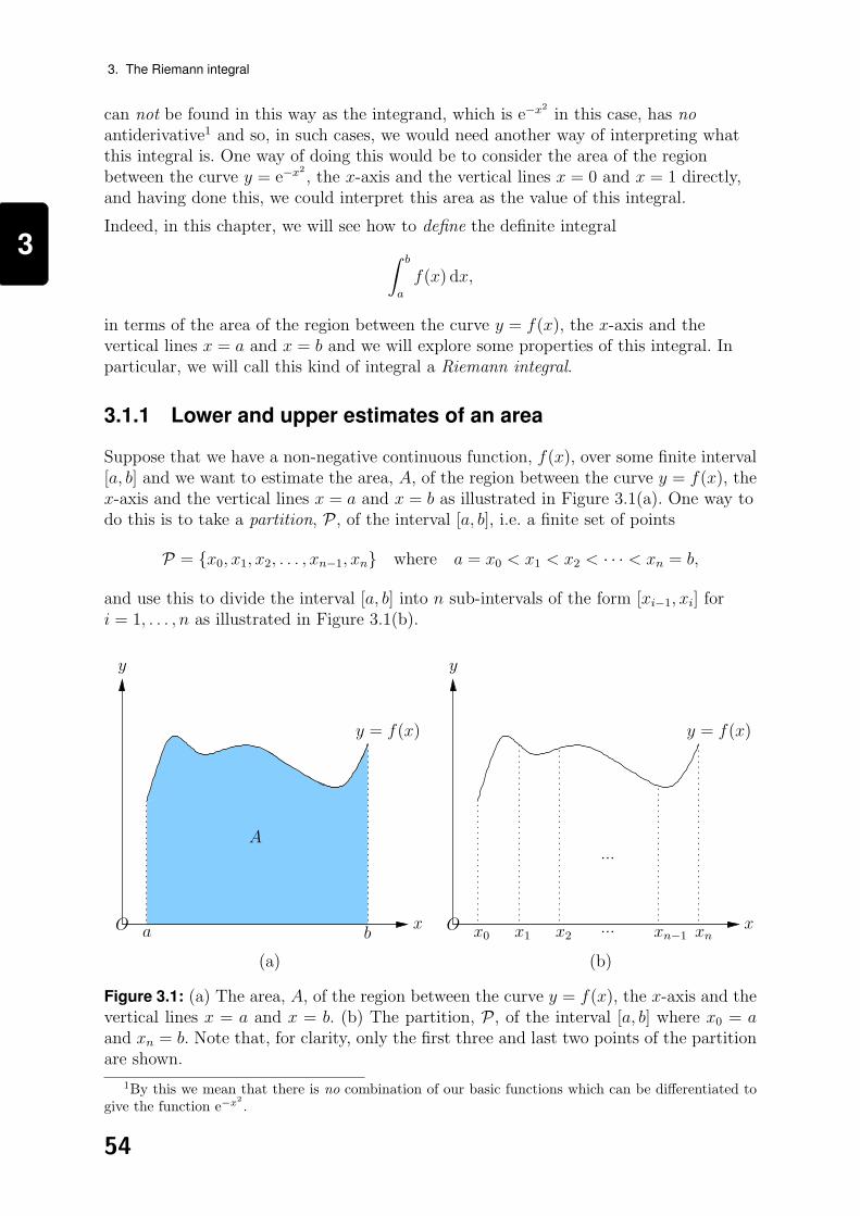
3

3. The Riemann integral

can not be found in this way as the integrand, which is e−x2

in this case, has noantiderivative1 and so, in such cases, we would need another way of interpreting whatthis integral is. One way of doing this would be to consider the area of the regionbetween the curve y = e−x

2, the x-axis and the vertical lines x = 0 and x = 1 directly,

and having done this, we could interpret this area as the value of this integral.

Indeed, in this chapter, we will see how to define the definite integral∫ b

a

f(x) dx,

in terms of the area of the region between the curve y = f(x), the x-axis and thevertical lines x = a and x = b and we will explore some properties of this integral. Inparticular, we will call this kind of integral a Riemann integral.

3.1.1 Lower and upper estimates of an area

Suppose that we have a non-negative continuous function, f(x), over some finite interval[a, b] and we want to estimate the area, A, of the region between the curve y = f(x), thex-axis and the vertical lines x = a and x = b as illustrated in Figure 3.1(a). One way todo this is to take a partition, P , of the interval [a, b], i.e. a finite set of points

P = {x0, x1, x2, . . . , xn−1, xn} where a = x0 < x1 < x2 < · · · < xn = b,

and use this to divide the interval [a, b] into n sub-intervals of the form [xi−1, xi] fori = 1, . . . , n as illustrated in Figure 3.1(b).

a

y = f(x)

b

y

xO

A

x0 x1 xnxn−1...x2

...

y = f(x)

y

xO

(a) (b)

Figure 3.1: (a) The area, A, of the region between the curve y = f(x), the x-axis and thevertical lines x = a and x = b. (b) The partition, P , of the interval [a, b] where x0 = aand xn = b. Note that, for clarity, only the first three and last two points of the partitionare shown.

1By this we mean that there is no combination of our basic functions which can be differentiated togive the function e−x

2

.

54

3

3.1. The Riemann integral

Each of these sub-intervals can then be taken to be the base of a rectangle whose heightin some way depends on the values of f(x) in that sub-interval. In particular, we cantake the height of the rectangle in each sub-interval to be the

minimum value of f(x) in that sub-interval so that the sum of the areas of theserectangles gives us a lower estimate of the area, or the

maximum value of f(x) in that sub-interval so that the sum of the areas of theserectangles gives us an upper estimate of the area.

Clearly, these rectangles will allow us to estimate the area of the region involved.Specifically, we can see that the

lower estimate, L(P), will be the sum of the areas of the rectangles illustrated inFigure 3.2(a), i.e.

L(P) =n∑i=1

Li,

and this will clearly be less than the area, A, that we are after as the rectanglesgive us ‘too little’ area if we compare their area with the area in Figure 3.1(a).

upper estimate, U(P), will be the sum of the areas of the rectangles illustrated inFigure 3.2(b), i.e.

U(P) =n∑i=1

Ui,

and this will clearly be greater than the area, A, that we are after as the rectanglesgive us ‘too much’ area if we compare their area with the area in Figure 3.1(a).

x0 x1 xnxn−1

L2 Ln

...x2

...L1

y = f(x)

y

xO x0 x1 xnxn−1

U2 Un

...x2

...U1

y = f(x)

y

xO

(a) (b)

Figure 3.2: In (a) and (b) we have, respectively, the rectangles that contribute towardsthe lower estimate, L(P), and the upper estimate, U(P), of A based on the partition P .Note that, for clarity, only the first, second and last rectangles are shown.

55

3


That is, we can see that using these estimates we have

L(P) < A < U(P),

and so these estimates provide us with bounds on the true value of A. Indeed, since it iseasy to work out the area of a rectangle using ‘base times height’, we can see that thebase of each of the rectangles is given by the length of the relevant sub-interval, i.e. fori = 1, 2, . . . , n we have a

sub-interval [xi−1, xi] with a length of xi − xi−1,

which means that, thinking about the heights as well, we have a

lower estimate given by

L(P) =n∑i=1

(xi − xi−1)mi,

where mi is the minimum value of f(x) for values of x in the sub-interval [xi−1, xi],i.e.

mi = min{f(x)|xi−1 ≤ x ≤ xi},is the height of this rectangle.

upper estimate given by

U(P) =n∑i=1

(xi − xi−1)Mi,

where Mi is the maximum value of f(x) for values of x in the sub-interval [xi−1, xi],i.e.

Mi = max{f(x)|xi−1 ≤ x ≤ xi},is the height of this rectangle.

Let’s have a look at a simple example to see how these estimates can be found inpractice.

Example 3.1 Suppose that we have the function f(x) = 1 + x2 defined over theinterval [−2, 2] and the partition P = {−2, 0, 1, 2} of this interval. Find the lowerand upper estimates, L(P) and U(P) respectively, of the area of the region boundedby the curve y = f(x), the x-axis and the vertical lines x = −2 and x = 2.

If we sketch the curve y = 1 + x2 over the interval [−2, 2] and indicate the points inthe partition P = {−2, 0, 1, 2} we see that we will be looking at three rectangleswhose bases are given by the sub-intervals [−2, 0], [0, 1] and [1, 2]. Indeed, for the

lower estimate, we need to sum the areas of the three rectangles illustrated inFigure 3.3(a) where the height of each rectangle is given by the minimum valueof f(x) in each of the sub-intervals. This gives us,

L(P) = (2)(1) + (1)(1) + (1)(2) = 5,

where we have taken each of the sub-intervals in turn and used ‘base timesheight’ to find the area of each rectangle.

56

3


upper estimate, we need to sum the areas of the three rectangles illustrated inFigure 3.3(b) where the height of each rectangle is given by the maximum valueof f(x) in each of the sub-intervals. This gives us,

U(P) = (2)(5) + (1)(2) + (1)(5) = 17,


In particular, observe that if A is the area of the region bounded by the curvey = 1 + x2, the x-axis and the vertical lines x = −2 and x = 2, then we can see fromthe illustrations in Figure 3.3 that we have

L(P) < A < U(P),

as we should expect from the lower and upper estimates respectively.

y = 1 + x2

y

x

1

2

2−2 1O

y = 1 + x2

y

x

1

2

2−2 1

5

O

(a) (b)

Figure 3.3: In (a) and (b) we have, respectively, the rectangles that contribute towardsthe lower estimate, L(P), and the upper estimate, U(P), of A based on the partition P .

Activity 3.1 Use integration to find the area, A, of the region bounded by thecurve y = 1 + x2, the x-axis and the vertical lines x = −2 and x = 2. Hence verifythat the lower and upper estimates found in Example 3.1 do indeed satisfy theinequality L(P) < A < U(P).

Of course, although we can find lower and upper estimates using simple partitions likethe one in Example 3.1, it will be necessary for us to use more sophisticated partitionsif we want to make any real progress towards more accurate estimates and, ultimately, adefinition of the Riemann integral.

57

3


Example 3.2 Suppose that we have the function f(x) = 1 + x defined over theinterval [0, 1] and the partitions

Pn ={

0, 1n, 2n, . . . , n−1

n, 1},

of this interval for some n ∈ N. Find the lower and upper estimates, L(Pn) andU(Pn) respectively, of the area of the region bounded by the curve y = f(x), thex-axis and the vertical lines x = 0 and x = 1.

If we sketch the curve y = 1 + x over the interval [0, 1] and indicate the points in thepartition Pn, we see that we will be looking at n rectangles whose bases are given bythe sub-intervals

[k−1n, kn

]for k = 1, 2, . . . , n. Indeed, we see that, for k = 1, 2, . . . , n,

each of these sub-intervals gives us a base whose length is

k

n− k − 1

n=

1

n,

and so, for the

lower estimate, we need to sum the areas of the n rectangles illustrated inFigure 3.4(a) where the height of each rectangle is given by the minimum valueof f(x) in each of the sub-intervals. This gives us,

L(Pn) =1

n

(1 +

0

n

)+

1

n

(1 +

1

n

)+

1

n

(1 +

2

n

)+ · · ·+ 1

n

(1 +

n− 1

n

),

where we have taken each of the sub-intervals in turn and used ‘base timesheight’ to find the area of each rectangle. Then, summing this series we find that

L(Pn) =1

2

(3− 1

n

),

as you can verify in Activity 3.2.

upper estimate, we need to sum the areas of the n rectangles illustrated inFigure 3.4(b) where the height of each rectangle is given by the maximum valueof f(x) in each of the sub-intervals. This gives us,

U(Pn) =1

n

(1 +

1

n

)+

1

n

(1 +

2

n

)+

1

n

(1 +

3

n

)+ · · ·+ 1

n

(1 +

n

n

),


U(Pn) =1

2

(3 +

1

n

),

as you can verify in Activity 3.2.

In particular, observe that if A is the area of the region bounded by the curvey = f(x), the x-axis and the vertical lines x = 0 and x = 1, then we can see from theillustrations in Figure 3.4 that we have

L(Pn) < A < U(Pn),

as we should expect from the lower and upper estimates respectively.

58

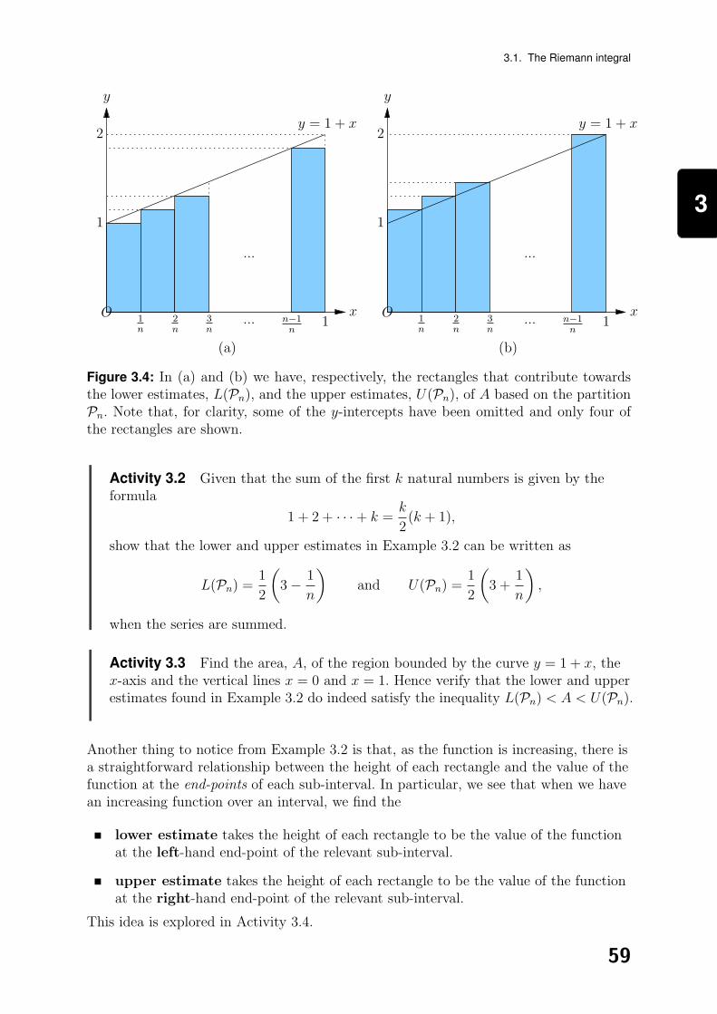
3


1n−1n

3n

2n

1

1n

2y = 1 + x

...

...

y

xO1n−1

n3n

2n

1

1n

2y = 1 + x

...

...

y

xO

(a) (b)

Figure 3.4: In (a) and (b) we have, respectively, the rectangles that contribute towardsthe lower estimates, L(Pn), and the upper estimates, U(Pn), of A based on the partitionPn. Note that, for clarity, some of the y-intercepts have been omitted and only four ofthe rectangles are shown.

Activity 3.2 Given that the sum of the first k natural numbers is given by theformula

1 + 2 + · · ·+ k =k

2(k + 1),

show that the lower and upper estimates in Example 3.2 can be written as

L(Pn) =1

2

(3− 1

n

)and U(Pn) =

1

2

(3 +

1

n

),

when the series are summed.

Activity 3.3 Find the area, A, of the region bounded by the curve y = 1 + x, thex-axis and the vertical lines x = 0 and x = 1. Hence verify that the lower and upperestimates found in Example 3.2 do indeed satisfy the inequality L(Pn) < A < U(Pn).

Another thing to notice from Example 3.2 is that, as the function is increasing, there isa straightforward relationship between the height of each rectangle and the value of thefunction at the end-points of each sub-interval. In particular, we see that when we havean increasing function over an interval, we find the

lower estimate takes the height of each rectangle to be the value of the functionat the left-hand end-point of the relevant sub-interval.

upper estimate takes the height of each rectangle to be the value of the functionat the right-hand end-point of the relevant sub-interval.

This idea is explored in Activity 3.4.

59

3


Activity 3.4 Suppose that f(x) is a non-negative continuous function defined oversome interval [a, b] and that P is the partition

{x0, x1, x2, . . . , xn−1, xn} where a = x0 < x1 < x2 < · · · < xn = b.

If f(x) is an increasing function on the interval [a, b], show that the lower and upperestimates, L(P) and U(P) respectively, of the area of the region bounded by thecurve y = f(x), the x-axis and the vertical lines x = a and x = b are given by

L(P) =n∑i=1

(xi − xi−1)f(xi−1) and U(P) =n∑i=1

(xi − xi−1)f(xi).

What are L(P) and U(P) if f(x) is a decreasing function on the interval [a, b]?

However, even though we can come up with such useful results about the lower andupper estimates of an area for increasing or decreasing functions over an interval,generally speaking, the best way to proceed is to sketch the relevant rectangles and thenuse these to infer their areas as we did in Examples 3.1 and 3.2.

3.1.2 Getting better lower and upper estimates

Having seen how to find lower and upper estimates of an area, we now want to see howwe can get better lower and upper estimates with a view to finding the best lower andupper estimates which should, naturally, be the value of the area itself. In particular, asthe next example makes clear, we should be able to get better lower and upperestimates by adding points to our partition so that we get ‘thinner’ rectangles and hencebetter estimates of the area involved.

Example 3.3 Use the partition P ′ = {−2,−1, 0, 1, 2} to find the lower and upperestimates, L(P ′) and U(P ′) respectively, of the area discussed in Example 3.1.Compare these values to what we found in that example.

If we sketch the curve y = 1 + x2 over the interval [−2, 2] and indicate the points inthe partition P ′ = {−2,−1, 0, 1, 2} we see that we will now be looking at fourrectangles whose bases are given by the sub-intervals [−2,−1], [−1, 0], [0, 1] and[1, 2]. Indeed, for the

lower estimate, we need to sum the areas of the four rectangles illustrated inFigure 3.5(a) where the height of each rectangle is given by the minimum valueof f(x) in each of the sub-intervals. This gives us,

L(P ′) = (1)(2) + (1)(1) + (1)(1) + (1)(2) = 6,


upper estimate, we need to sum the areas of the four rectangles illustrated inFigure 3.5(b) where the height of each rectangle is given by the maximum value

60

3


of f(x) in each of the sub-intervals. This gives us,

U(P ′) = (1)(5) + (1)(2) + (1)(2) + (1)(5) = 14,


Comparing this with our answers from Example 3.1, we can see that the

lower estimates give us

L(P) = 5 < 6 = L(P ′) =⇒ L(P) < L(P ′),

i.e. L(P ′) is a larger, and hence better, lower estimate of the area than L(P).

upper estimates give us

U(P ′) = 14 < 17 = U(P) =⇒ U(P ′) < U(P),

i.e. U(P ′) is a smaller, and hence better, upper estimate of the area than U(P).

Indeed, it should be clear that this improvement in the lower and upper estimateshas come about because P ′ has one more point than P and this has enabled us toreplace the single rectangle for the sub-interval [−2, 0] from P (see Figure 3.3) withtwo ‘thinner’ rectangles for the sub-intervals [−2,−1] and [−1, 0] from P ′ (seeFigure 3.5).

In particular, observe that if A is the area of the region bounded by the curvey = 1 + x2, the x-axis and the vertical lines x = −2 and x = 2, then we can see fromthe results above and the illustrations in Figure 3.5 that we have

L(P) < L(P ′) < A < U(P ′) < U(P),

i.e. P ′ gives us better lower and upper estimates of A than P .

Activity 3.5 Use your answer to Activity 3.1 to verify that the lower and upperestimates found in Example 3.2 satisfy the inequality

L(P) < L(P ′) < A < U(P ′) < U(P),

as one would expect.

In fact, this is what we should expect more generally, i.e.

lower (and upper) estimates should always be less (or greater) than the area theyare estimates of, and

increasing the number of the points in the partition should always give us betterlower (or upper) estimates.

To make this clear, let’s consider another example.

61

3


y = 1 + x2

y

x

1

2

2−2 1−1O

y = 1 + x2

y

x

1

2

2−2 1−1

5

O

(a) (b)

Figure 3.5: In (a) and (b) we have, respectively, the rectangles that contribute towardsthe lower estimate, L(P ′), and the upper estimate, U(P ′), of A based on the partition P .

Example 3.4 Use the results from Example 3.2 to verify the two points above.

We start by noting that in this case, as we saw in Activity 3.3, we can meaningfullytalk about the value of the area, A, of the region bounded by the curve y = 1 + x,the x-axis and the vertical lines x = 0 and x = 1 because it is simply the area of atrapezium. Indeed, for the first point, we have already shown in Activity 3.3 that

L(Pn) < A < U(Pn),

i.e. if we are estimating the area A, then whatever value of n ∈ N we take, the lowerestimates, L(Pn), are always less than A whereas the upper estimates, U(Pn) arealways greater than A.

For the second point, consider that the partition, Pn has n+ 1 points and, if we takesome other natural number m > n, the partition Pm will have m+ 1 points, i.e. Pmhas m− n more points than Pn. We then have

lower estimates given by

L(Pn) =1

2

(3− 1

n

)and L(Pm) =

1

2

(3− 1

m

).

But, m > n > 0 means that

1

n>

1

m=⇒ 3− 1

n< 3− 1

m=⇒ 1

2

(3− 1

n

)<

1

2

(3− 1

m

),

which means that we have L(Pn) < L(Pm). Indeed, using the first point, both ofthese lower estimates must be less than A, and so we have

L(Pn) < L(Pm) < A,

i.e. increasing the number of points in the partition has given us a better lowerestimate.

62

3


upper estimates given by

U(Pn) =1

2

(3 +

1

n

)and U(Pm) =

1

2

(3 +

1

m

).

But, m > n > 0 means that

1

n>

1

m=⇒ 3 +

1

n> 3 +

1

m=⇒ 1

2

(3 +

1

n

)>

1

2

(3 +

1

m

),

which means that we have U(Pn) > U(Pm). Indeed, using the first point, bothof these upper estimates must be greater than A, and so we have

U(Pn) > U(Pm) > A,

i.e. increasing the number of points in the partition has given us a better upperestimate.

Notice, however, that although we have been using various graphical and geometric‘intuitions’ about the area under a curve in our examples, we have not actually definedwhat the area under a curve is. In particular, this is why all reference to using definiteintegrals to find areas have been relegated to Activities 3.1 and 3.3 where they can serveto illustrate the points being made without interfering with the flow of our argument.

3.1.3 The definition of the Riemann integral

We now turn to the definition of the Riemann integral which will allow us to assign avalue to the definite integral ∫ b

a

f(x) dx,

where f(x) is a non-negative continuous function over the interval [a, b] by taking it tobe the value of the area of the region between the curve y = f(x), the x-axis and thevertical lines x = a and x = b. So, we have to ask ourselves, what is the value of thisarea?

It should be clear, from what we have seen above, that in the case we are considering:

Every partition of [a, b] gives us a lower and upper estimate of the area.

Every lower estimate is less than every upper estimate, i.e. we have L(P) ≤ U(P).

This means that there is at least one number A such that L(P) ≤ A ≤ U(P).

Now, if there is only one such number, then A is the value of the area and hence thevalue of the Riemann integral ∫ b

a

f(x) dx,

whereas if there is more than one such number, then we say that the area is undefinedand so this Riemann integral is undefined too.

63

3


In practice, we can use this to find the value of the Riemann integral,

I =

∫ b

a

f(x) dx,

where f(x) is a non-negative continuous function as follows. We find the lower andupper estimates in terms of some appropriately general partition, P , and then find the

smallest number, L∗, that is greater than all the lower estimates, L(P), and the

largest number, U∗, that is smaller than all the upper estimates, U(P).

Then, according to what we have seen above, we should find that

L∗ ≤ I ≤ U∗,

so that, if there is only one number, I, that satisfies this inequality we can take this tobe the value of the Riemann integral.2

Example 3.5 Continuing on from Examples 3.2 and 3.4, find the value of∫ 1

0

(1 + x) dx,

using the definition of the Riemann integral.

We saw in Example 3.2 that we have

lower estimates given by

L(Pn) =1

2

(3− 1

n

)≤ 3

2.

for all n ∈ N. That is, following on from Example 3.4, we have found that, form,n ∈ N with m > n,

L(Pn) ≤ L(Pm) ≤ L∗,

where L∗ = 3/2 is the smallest number that is greater than all the lowerbounds.3

upper estimates given by

U(Pn) =1

2

(3 +

1

n

)≥ 3

2,

2Technically, we are looking at every possible partition, P, of the interval [a, b] and, having found thecorresponding lower and upper estimates, we take L∗ to be the least upper bound (or supremum) of thelower estimates and U∗ to be the greatest lower bound (or infimum) of the upper estimates, i.e.

L∗ = sup{L(P)|P is a partition of [a, b]} and U∗ = inf{U(P)|P is a partition of [a, b]}.

This is because, generally, as we have taken a partition to be a finite set of points, we shall find thatthere is no partition P that makes L∗ = L(P) or U∗ = U(P), even though L∗ and U∗ act as the relevantbounds on L(P) and U(P) respectively.

64

3


for all n ∈ N. That is, following on from Example 3.4, we have found that, form,n ∈ N with m > n,

U∗ ≤ U(Pm) ≤ U(Pn),

where U∗ = 3/2 is the largest number that is smaller than all the upper bounds.

This means that there is only one number, I, that satisfies the inequality

L∗ ≤ I ≤ U∗,

in this case, i.e. I = 3/2, and so we take this to be the value of the given Riemannintegral. That is, ∫ 1

0

(1 + x) dx =3

2,

as we should expect from Activity 3.3.

Activity 3.6 Use the definition of the Riemann integral to find the value of∫ 2

0

(1 + x2) dx,

by considering, for m ∈ N, the partition

Pm = {0, 1m, 2m, . . . , 2m−1

m, 2},

of the interval [0, 2].

Note: You will need to use the formula

12 + 22 + · · ·+ k2 =k

6(k + 1)(2k + 1),

for the sum of the first k square numbers.

Of course, more generally, we should expect the Riemann integral∫ b

a

f(x) dx,

to be well-defined if f(x) is a non-negative continuous function over the interval [a, b].This is because it is just the area between the curve y = f(x), the x-axis and thevertical lines x = a and x = b, which is clearly well-defined if f(x) is continuous. Indeed,although we do not dwell on this here, we can drop the requirement that f(x) isnon-negative and extend what we have seen to functions where f(x) is negative forsome values of x in the interval [a, b] by utilising the methods discussed in Section 5.3 of174 Calculus. All of this leads to the following fact.

3That is, we haveL∗ = sup{L(Pn)|n ∈ N},

as, for all n ∈ N, L(Pn) ≤ L∗ and so L∗ is an upper bound on the lower estimates and L∗ is the leastupper bound as there is no other upper bound, l, such that l < L∗. Also observe that, for any n ∈ N,L(Pn) < L∗ and so there is no partition with a finite number of points that makes L(Pn) = L∗.

65

3


If f(x) is a continuous function over the interval [a, b], then the Riemannintegral ∫ b

a

f(x) dx,

exists.

Although, we shall not prove this here.

3.1.4 What happens if the integrand isn’t continuous?

We now begin to consider the Riemann integral∫ b

a

f(x) dx,

when f(x) is not continuous over the interval [a, b]. In particular, we consider how thedefinition needs to be slightly modified when the integrand has finite discontinuities atcertain points and encounter a case where the Riemann integral is undefined.

In particular, one problem we will encounter is that a function which has finitediscontinuities may not have a minimum or maximum value over every interval. Tomotivate the discussion that follows, let’s look at an example.

Example 3.6 Consider the integral∫ 1

0

f(x) dx where f(x) =

{2x if 0 ≤ x < 1

1 if x = 1

and, for n ∈ N, the partition

Pn = {0, 1n, 2n, . . . , 1},

of the interval [0, 1]. Sketch f(x) over the interval [0, 1] and explain why the upperestimates (as we defined them in Section 3.1.1) are problematic in this case. Doesthis seem reasonable?

If we sketch f(x) over the interval [0, 1], as illustrated in Figure 3.6(a), we see thatthe function has a finite discontinuity at x = 1 because f(x)→ 2 as x→ 1− butf(1) = 1 6= 2. In particular, even though f(x)→ 2 as x→ 1−, the function neverattains the value two and so, over the interval [0, 1], this function has no maximumvalue.4

This poses a problem for the upper estimates since, if we consider the sub-interval[n−1n, 1], as illustrated in Figure 3.6(b), it means that we can not ascribe a value to

Mn = max{f(x)|n−1n≤ x ≤ 1},

and so, bearing in mind that the base of each rectangle that arises from the partitionis 1/n, the upper estimates

U(Pn) =n∑i=1

1

nMi,

66

3


for n ∈ N are not defined since we cannot ascribe a value to its last term.

However, given that we want to interpret the given Riemann integral as the area ofthe region under the curve y = f(x), the x-axis and the vertical lines x = 0 andx = 1, we would surely expect this area to exist. Indeed, we would expect this to bethe area of a triangular region which, using ‘half base times height’, is one! So, inthis case, it seems unreasonable that the Riemann integral does not exist because wecan not define its upper estimates.

1

1

2y = f(x)

y

xO 1n−1n

1

2y = f(x)

y

xO

(a) (b)

Figure 3.6: In (a) we have a sketch of the function y = f(x) from Example 3.6 and in (b)we examine the effect of the problematic sub-interval [n−1

n, 1].

To deal with cases like this, we should use a slightly more general definition of theRiemann integral ∫ b

a

f(x) dx,

in terms of a partition, P , of the interval [a, b] given by

P = {x0, x1, x2, . . . , xn−1, xn} where a = x0 < x1 < x2 < · · · < xn = b,

which runs as before except that, now, we have

lower estimates, L(P), given by

L(P) =n∑i=1

(xi − xi−1)mi,

where mi is the greatest lower bound, or infimum, of f(x) for values of x in thesub-interval [xi−1, xi], i.e.

mi = inf{f(x)|xi−1 ≤ x ≤ xi},4Of course, the function g(x) = 2x defined over the interval [0, 1] gives us g(1) = 2 and this is its

maximum value, but the function f(x) that we are considering here has f(1) = 1!

67

3


with the understanding that, in cases where this value is actually attained by thefunction in the sub-interval, this will just be the minimum value of the function asbefore.

upper estimates, U(P), given by

U(P) =n∑i=1

(xi − xi−1)Mi,

where Mi is the supremum of f(x) for values of x in the sub-interval [xi−1, xi], i.e.

Mi = sup{f(x)|xi−1 ≤ x ≤ xi},with the understanding that, in cases where this value is actually attained by thefunction in the sub-interval, this will just be the maximum value of the function asbefore.

Of course, with this in mind, we can now make sense of what we saw in Example 3.6 asthe next example shows.

Example 3.7 Following on from Example 3.6, use this more general definition ofthe Riemann integral to find the value of∫ 1

0


{2x if 0 ≤ x < 1

1 if x = 1

by considering, for n ∈ N with n ≥ 2, the partitions

Pn = {0, 1n, 2n, . . . , 1},

of the interval [0, 1].

If we sketch the curve y = f(x) over the interval [0, 1] and indicate the points in thepartition Pn we see that we will be looking at n rectangles whose bases are given bythe sub-intervals

[k−1n, kn

]for k = 1, 2, . . . , n. Indeed, we see that, for k = 1, 2, . . . , n,


k

n− k − 1

n=

1

n,

and so, for the

lower estimates, we need to sum the areas of the n rectangles illustrated inFigure 3.7(a) where the height of each rectangle is given by the minimum valueof f(x) in each of the sub-intervals. This gives us,

L(Pn) =1

n

(2 · 0

n

)+

1

n

(2 · 1

n

)+

1

n

(2 · 2

n

)+ · · ·+ 1

n

(2 · n− 2

n

)+

1

n

(1

),


L(Pn) = 1− 2 · n− 1

n2≤ 1,

for n ≥ 2, as you can verify in Activity 3.7. That is, L∗ = 1 is the smallestnumber that is greater than all the lower bounds.

68

3


upper estimates, we need to sum the areas of the n rectangles illustrated inFigure 3.7(b) where the height of each rectangle is given by the maximum valueof f(x) in the first n− 1 sub-intervals and the supremum of f(x) in the lastsub-interval. This gives us,

U(Pn) =1

n

(2 · 1

n

)+

1

n

(2 · 2

n

)+

1

n

(2 · 3

n

)+ · · ·+ 1

n

(2 · n− 1

n

)+

1

n

(2 · nn

),


U(Pn) = 1 +1

n≥ 1,

for n ≥ 2, as you can verify in Activity 3.7. That is, U∗ = 1 is the largestnumber that is less than all the upper bounds.


L∗ ≤ I ≤ U∗,

in this case, i.e. I = 1, and so we take this to be the value of the given Riemannintegral. That is,∫ 1

0

f(x) dx = 1 when f(x) =

{2x if 0 ≤ x < 1,

1 if x = 1,

as we should expect from our discussion in Example 3.6.

Activity 3.7 Using the formula for the sum of the first k natural numbers given inActivity 3.2, show that the lower and upper estimates in Example 3.7 can be writtenas

L(Pn) = 1− 2 · n− 1

n2and U(Pn) = 1 +

1

n,

when the series are summed and verify that, for n ≥ 2, we have L(Pn) ≤ 1 andU(Pn) ≥ 1.

However, if there are too many finite discontinuities, the Riemann integral will not existas the next example shows.

Example 3.8 Consider the integral∫ 1

0


{1 if x is rational,

0 if x is irrational,

and the partition

P = {x0, x1, x2, . . . , xn−1, xn} where 0 = x0 < x1 < x2 < · · · < xn−1 < xn = 1,

69

3


n−2n

1n−1n

3n

2n

1

1n

2y = f(x)

...

...

y

xOn−2n

1n−1n

3n

2n

1

1n

2y = f(x)

...

...

y

xO

(a) (b)

Figure 3.7: In (a) and (b) we have, respectively, the rectangles that contribute towardsthe lower estimates, L(Pn), and the upper estimates, U(Pn), of the Riemann integral inExample 3.7 based on the partition Pn for n ≥ 2. Note that, for clarity, some of they-intercepts have been omitted and only five of the rectangles are shown. (Of course, in(a), the first rectangle has a height of zero and so we can not see it!)

of the interval [0, 1]. Find the lower and upper estimates, L(P) and U(P)respectively, of this integral. What do these tell you about the existence of thisRiemann integral?

Note: A real number is said to be rational if it is of the form p/q where p, q ∈ Z andq 6= 0 and, if it is not rational, a number is said to be irrational.5 Indeed, we willneed the facts that

(1) every interval [a, b] with a < b contains at least one rational number, and

(2) every interval [a, b] with a < b contains at least one irrational number,

to answer this question.

In this case, we can not sketch the function as it is discontinuous at every point, butwe can easily find the

lower estimate by noting that in every sub-interval [xi−1, xi] of lengthxi − xi−1 the minimum value of f(x) is zero as, by fact (1), there is at least onerational number in that sub-interval. This gives us

L(P) = (x1− x0)(0) + (x2− x1)(0) + · · ·+ (xn−1− xn−2)(0) + (xn− xn−1)(0) = 0,

i.e. the lower estimate is zero for any partition, P .

upper estimate by noting that in every sub-interval [xi−1, xi] of lengthxi − xi−1 the maximum value of f(x) is one as, by fact (2), there is at least oneirrational number in that sub-interval. This gives us

U(P) = (x1−x0)(1)+(x2−x1)(1)+· · ·+(xn−1−xn−2)(1)+(xn−xn−1)(1) = xn−x0,

70

3


if we cancel the corresponding intermediate terms and, noting that x0 = 0 andxn = 1, we then see that the upper estimate is one for any partition, P .

Consequently, we see that as L(P) = 0 and U(P) = 1 for any partition P , there aremany numbers I that satisfy the inequality

L(P) ≤ I ≤ U(P),

and so, as there is not only one such number, we can not assign a single value to thisRiemann integral, i.e. it does not exist.6

In the next chapter, we will see how to deal with Riemann integrals in cases where theinterval we are concerned with is not finite and where the integrand fails to becontinuous in other, less straightforward, ways (such as the presence of an infinitediscontinuity).

3.1.5 Some properties of the Riemann integral

So far, we have been concerned with Riemann integrals of the form∫ b

a

f(x) dx,

where a < b and we now want to extend our understanding of such integrals by seeingwhat happens when a = b or a > b. To do this, we introduce some basic properties ofthe Riemann integral in Theorem 3.1 and, in particular, these will be useful in the nextsection.

Theorem 3.1 If the Riemann integral of f exists over some interval containing thepoints a, b and c with a ≤ c ≤ b, then

(a) The integral over an interval of zero length is zero, i.e.∫ a

a

f(x) dx = 0.

(b) The integral is additive over the interval of integration, i.e.∫ b

a

f(x) dx =

∫ c

a

f(x) dx+

∫ b

c

f(x) dx.

(c) Interchanging the limits of integration changes the sign of the integral, i.e.∫ b

a

f(x) dx = −∫ a

b

f(x) dx.

5For example, you may have encountered the fact that the real number,√

2, is irrational because itcan not be written in the form p/q where p, q ∈ Z and q 6= 0.

6Actually, there is a well-defined sense in which ‘almost all’ real numbers are irrational and so thevalue of this integral ‘ought’ to be zero as its value shouldn’t be affected by the value of the integrandat a ‘few’ points where its argument is rational. Indeed, although it is beyond the scope of this course,you might care to note that there is a more general notion of integration, called the Lebesgue integral,whose value would be zero in this case.

71

3


(d) It follows that ∫ b

a

f(x) dx =

∫ b

c

f(x) dx−∫ a

c

f(x) dx.

We will not prove this theorem here but, in Activity 3.8, you will be able to motivatethese results by appealing to our interpretation of the Riemann integral as an area.

Activity 3.8 Suppose that f is a non-negative function whose Riemann integralexists over some interval containing the points a, b and c. By considering the areasinvolved, explain why parts (a) and (b) of Theorem 3.1 hold. Hence deduce parts (c)and (d) of this theorem.

3.2 The Fundamental Theorem of Calculus

Returning to the case where the function, f(x), is continuous and non-negative over aninterval [a, b], we have defined the Riemann integral,∫ b

a

f(x) dx,

in terms of the area between the curve y = f(x), the x-axis and the vertical lines x = aand x = b. What we want to do now is make sure that this view of integration agreeswith what we saw in Chapter 5 of 174 Calculus. In particular, we want to be sure thatthe relationship between integrals and derivatives that we used there still works ifintegration is defined in this way. Indeed, the key result here is the FundamentalTheorem of Calculus (which we will abbreviate to FTC) and this runs as follows.

Theorem 3.2 (FTC) If f is a continuous function defined on the interval [a, b], then

d

dt

(∫ t

c

f(x) dx

)= f(t),

for any numbers c and t in the interval (a, b).

We will spend the rest of this chapter seeing why this works and what it tells us aboutthe relationship between integrals and derivatives.

3.2.1 Motivating the FTC

To see how the FTC arises, consider the case where f(x) is a decreasing non-negativecontinuous function over the interval [a, b]. In particular, we will take c, t ∈ (a, b) wherex > c and consider the integral

A(t) =

∫ t

c

f(x) dx,

so that A(t) represents the area between the curve y = f(x), the x-axis and the verticallines x = c and x = t as illustrated in Figure 3.8(a). Indeed, this means that if h > 0, we

72

3

3.2. The Fundamental Theorem of Calculus

also have the integral

A(t+ h) =

∫ t+h

c

f(x) dx,

so that A(t) represents the area between the curve y = f(x), the x-axis and the verticallines x = c and x = t+ h as illustrated in Figure 3.8(b).

y = f(x)

A(t)

y

xOa btc

y = f(x)

A(t+ h)

t+ h

y

xOa btc

(a) (b)

Figure 3.8: The shaded regions in (a) and (b) have areas A(t) and A(t+ h) respectively.

We now consider the difference between these two areas, i.e. the quantity

A(t+ h)− A(t),

which is the area of the vertically hatched region indicated in Figure 3.9.

��

��

��

��

�� y = f(x)

t+ h

y

xOa btc ��

��

�� y = f(x)

t+ h

y

xOa btc

(a) (b)

Figure 3.9: The areas of the shaded regions in (a) and (b) are the lower and upperestimates, respectively, of the area A(t+ h)− A(t) of the vertically hatched region.

73

3


In particular, we see that since f(x) is a decreasing function over the interval [a, b], wehave a

lower estimate of this area given by the area of the shaded rectangle inFigure 3.9(a) which, using ‘base times height’, is

hf(t+ h),

and so we have hf(t+ h) ≤ A(t+ h)− A(t).

upper estimate of this area given by the area of the shaded rectangle inFigure 3.9(b) which, using ‘base times height’, is

hf(t),

and so we have A(t+ h)− A(t) ≤ hf(t).

Consequently, putting these two inequalities together, we have

hf(t+ h) ≤ A(t+ h)− A(t) ≤ hf(t) =⇒ f(t+ h) ≤ A(t+ h)− A(t)

h≤ f(t),

as h > 0. Then, we take the limit as h→ 0+ on both sides of this inequality to get

limh→0+

f(t+h) ≤ limh→0+

A(t+ h)− A(t)

h≤ lim

h→0+f(t) =⇒ f(t) ≤ lim

h→0+

A(t+ h)− A(t)

h≤ f(t),

if we use the continuity of f(x) over [a, b].7 This means that

limh→0+

A(t+ h)− A(t)

h= f(t),

and, repeating the argument with h < 0, we also get

limh→0−

A(t+ h)− A(t)

h= f(t),

as you can verify in Activity 3.9. Then, putting these two results together, we have

limh→0

A(t+ h)− A(t)

h= f(t) =⇒ A′(t) = f(t),

if we use the definition of the derivative, A′(t), of A(t). Thus, we have shown that whenf(x) is a continuous decreasing function over [a, b] with c, t ∈ (a, b) and c < t, we have

A′(t) =d

dt

(∫ t

c

f(x) dx

)= f(t),

as expected from the FTC.

7Notice that the continuity of f(x) over [a, b] is essential here in order to justify the assertion thatthe limit

limh→0+

f(t+ h),

exists and that it is equal to f(t). Also, notice that we can only take the limit as h → 0+ here as wehave assumed that h > 0.

74

3


Activity 3.9 Show that

limh→0−

A(t+ h)− A(t)

h= f(t),

using an argument similar to the one above with h < 0.

3.2.2 Notation: Dummy variables

Before we proceed, we should make sure that we understand the role that dummyvariables are playing here. Generally, given a function, f , defined over some interval[a, b] it makes no difference what we call the independent variable. That is, we could usex and look at values of

f(x) where x ∈ [a, b],

or we could use y and look at values of

f(y) where y ∈ [a, b],

or we could use any other letter to represent the independent variable.8 Indeed, whenwe look at an integral like ∫ b

a

f(x) dx,

where a and b are constants, we know that the answer will not depend on x and, inparticular, it makes no difference if we write this integral as∫ b

a

f(y) dy.

In such cases, the variable that is used inside the integral is a dummy variable as it doesnot matter what we call it since it does not occur in the final answer. However, when wehave an integral like ∫ t

c

f(x) dx,

where only c is a constant, we now have two variables. One of these variables, x, is adummy variable as it will not figure in the final answer but the other variable, t, is notas the answer will be a function of t, i.e. we may write

F (t) =

∫ t

c

f(x) dx.

Of course, this means that ∫ t

c

f(x) dx and

∫ t

c

f(y) dy,

say, represent the same integral whereas

F (t) =

∫ t

c

f(x) dx and F (s) =

∫ s

c

f(x) dx,

8Although, by convention, we usually use letters from the end of the English alphabet to denotevariables.

75

3


say, represent the same function, namely F . In particular, this means that some caremust be taken when choosing names for our variables as we would not want to write

F (x) =

∫ x

c

f(x) dx,

because this uses x as both the independent variable of F and the dummy variable ofthe integral. To see why this is a problem, ask yourself what is, say, F (1) using thisdefinition of F? Is it ∫ 1

c

f(x) dx or

∫ 1

c

f(1) d1 ?

Obviously, we want to be able to distinguish between these two options and that is whywe use dummy variables!

3.2.3 The relationship between integration and differentiation

Having motivated the FTC, we are now in a position to clarify the relationship betweenintegration and differentiation. That is, we want to find that differentiation ‘undoes’integration and that, up to an arbitrary constant, integration ‘undoes’ differentiation.

Differentiation ‘undoes’ integration

Recall that, in Section 5.1 of 174 Calculus, we defined an antiderivative of the function,f(t), to be a function F (t) such that

dF

dt= f(t).

Indeed, using the FTC, we can now see that the integral

F (t) =

∫ t

c

f(x) dx,

where c is a constant is an antiderivative of f(t) since

F ′(t) =dF

dt=

d

dt

(∫ t

c

f(x) dx

)= f(t).

That is, differentiation ‘undoes’ (or ‘reverses’) the process of integration as, given theintegral of f , differentiation allows us to find f .

Integration ‘undoes’ differentiation

Conversely, if F (t) is an antiderivative of f(t), say we have

F (t) =

∫ t

c

f(x) dx,

where c is a constant, as before, then for some constant d, we also have∫ t

d

f(x) dx =

∫ t

c

f(x) dx−∫ d

c

f(x) dx = F (t)− F (d),

76

3


using Theorem 3.1(d) and, of course, F (d) is a constant. That is, integration ‘undoes’(or ‘reverses’) the process of differentiation as, given the derivative of F , i.e. f ,integration allows us to find F up to a constant. Indeed, we find that if F1(t) and F2(t)are any two antiderivatives of f , we have

F ′1(t) = f(t) and F ′2(t) = f(t),

which means that

d

dt

(F1(t)− F2(t)

)= F ′1(t)− F ′2(t) = f(t)− f(t) = 0,

and so the function F1(t)− F2(t) must be a constant as its derivative is zero.Consequently, any two antiderivatives of f can only differ by a constant and so, as weshould expect, integration only ‘undoes’ differentiation up to an arbitrary constant.

In summary

Having established that the expected relationships between integration anddifferentiation hold, we can now evaluate Riemann integrals in the manner described inChapter 5 of 174 Calculus, i.e. we can use our standard integrals and rules ofintegration.

3.2.4 Some applications of the FTC

We are now in a position to consider some other applications of the FTC.

Using the FTC and Taylor series to approximate the value of an integral

At the beginning of this chapter, we observed that the integral∫ 1

0

e−x2

dx,

could not be found in the standard way as the integrand, e−x2, has no antiderivative. Of

course, we could use our interpretation of the integral as an area to gain someapproximation to the value of this integral, but the FTC allows us to approximate itsvalue in another way as the next example shows.

Example 3.9 Given that

F (t) =

∫ t

0

e−x2

dx,

find the Taylor series for F (t) about t = 0 in terms up to t3. Hence find anapproximate value for F (1).

To find the Taylor series for F (t) about t = 0, we note that

F (t) =

∫ t

0

e−x2

dx =⇒ F (0) =

∫ 0

0

e−x2

dx = 0,

77

3


using Theorem 3.1(a) and that

F ′(t) =d

dt

(∫ t

0

e−x2

dx

)= e−t

2

=⇒ F ′(0) = 1,

using the FTC. We then see that,

F ′′(t) = −2t e−t2

=⇒ F ′′′(t) = (−2)(e−t2

) + (−2t)(−2t e−t2

) = 2(2t2 − 1) e−t2

,

which means that F ′′(0) = 0 and F ′′′(0) = −2. Thus, we have

F (t) = F (0) + tF ′(0) +t2

2!F ′′(0) +

t3

3!F ′′′(0) + · · · = t− t3

3+ · · · ,

as the Taylor series for F (t) about t = 0 in terms up to t3. Consequently, we can seethat

F (1) ' 1− 1

3=

2

3,

is the required approximate value for F (1). Indeed, as

F (1) =

∫ 1

0

e−x2

dx,

this gives us an approximate value of 0.67 (2dp) for this integral and this is fairlyclose to the true value which turns out to be 0.75 (2dp).

Using the FTC to define functions in terms of definite integrals

We can also use the FTC to define certain functions in terms of definite integrals as thenext activity shows.

Activity 3.10 The function, F (x), satisfies the conditions F ′(x) = e−x2

andF (0) = 0. Write F (x) as a definite integral of the form

F (x) =

∫ x

A

f(t) dt,

for a suitable choice of f and A.

Using the FTC to solve integral equations

We can also use the FTC to solve certain integral equations, i.e. equations that involvedefinite integrals, as the next example shows.

Example 3.10 Use the FTC to solve the integral equation f(t) = 1−∫ t

0

f(x) dx.

If we differentiate both sides of this integral equation with respect to t, we get

f ′(t) = −f(t),

78

3


where we have used the FTC to differentiate the integral. Solving this simpleseparable differential equation in the standard way9 we get

f(t) = A e−t,

for some constant A ∈ R. Indeed, setting t = 0 in the integral equation, we see that

f(0) = 1−∫ 0

0

f(x) dx =⇒ f(0) = 1− 0 = 1,

using Theorem 3.1(a), and so A = 1. Consequently, a function f that satisfies thisintegral equation is

f(t) = e−t,

and so this is the required solution.

In fact, we will see another way of solving integral equations like this in Chapter 7 whenwe look at Laplace transforms.

3.2.5 An extension of the FTC

We can also use the FTC to differentiate more complicated integrals if we use the chainrule. For instance, if we have the integral

F (t) =

∫ q(t)

p(t)

f(x) dx,

we can use Theorem 3.1(d) to write it as

F (t) =

∫ q(t)

c

f(x) dx−∫ p(t)

c

f(x) dx,

where c is some constant. Then, differentiating both sides of this expression withrespect to t, we get

F ′(t) =d

dt

(∫ q(t)

c

f(x) dx

)− d

dt

(∫ p(t)

c

f(x) dx

),

so that, using the chain rule, we have

F ′(t) =dq

dt

d

dq

(∫ q

c

f(x) dx

)− dp

dt

d

dp

(∫ p

c

f(x) dx

).

Then, applying the FTC, this gives us

F ′(t) =d

dt

∫ q(t)

p(t)

f(x) dx = q′(t)f(q(t))− p′(t)f(p(t)),

where, of course, this result assumes that p and q are both differentiable functions of tand that f is continuous over the two intervals of integration. Let’s look at an exampleto see how this works.

9See, for example, Section 8.2.1 of 174 Calculus.

79

3


Example 3.11 Given that

F (t) =

∫ t3

4t

x2 dx,

find F ′(t) using the result above.

Here we have p(t) = 4t and q(t) = t3, which means that

F ′(t) = (3t2)(t3)2 − (4)(4t)2 = 3t8 − 64t2,

if we use the result above.

Activity 3.11 Following on from Example 3.11, use integration to find F (t) andhence verify your answer for F ′(t).

Indeed, we will see in Section 6.1.3 that this result can be extended even further whenwe meet the Leibniz rule for differentiating integrals.

Using the FTC to derive identities

This extension of the FTC also has an interesting application because it can be used toderive certain identities like the ones we saw in Section 2.1.4 of 174 Calculus.

Example 3.12 Use integration to verify that

ln t =

∫ t

1

1

xdx,

where t > 0. Hence show that if a > 0 is a constant and F is given by

F (t) = ln(at)− ln t,

where t > 0, then F ′(t) is zero. Deduce that F (t) is a constant and, by finding thisconstant, deduce that

ln(ab) = ln a+ ln b,

where b > 0 is a constant too.

Note: Of course, if we use the fact that

ln(ab) = ln a+ ln b =⇒ ln(ab)− ln b = ln a,

for a, b > 0, then it is obvious that

F (t) = ln(at)− ln t = ln a,

for a, t > 0. Indeed, as a is a constant, this means that F (t) = ln a is a constant tooand so, obviously, F ′(t) = 0! However, here we are using an integral that representslnx and the function F (t) to derive this fact and so we can not use it in this wayhere.

80

3


Firstly, it is easy to verify that, for t > 0, we have∫ t

1

1

xdx =

[lnx

]t1

= ln t− ln 1 = ln t,

as ln 1 = 0. Then, for a, t > 0, we can use this to write

F (t) = ln(at)− ln t =

∫ at

1

1

xdx−

∫ t

1

1

xdx,

so that, using the FTC and its extension as appropriate, we have

F ′(t) = (a)

(1

at

)− 1

t=

1

t− 1

t= 0,

as required. But, of course, if F ′(t) = 0, this means that F (t) = c where c is aconstant which we can find by taking any value of t > 0. So, if we let t = 1, say, wehave

c = F (1) = ln a− ln 1 = ln a,

as the value of the constant. Consequently, we have

F (t) = ln a = ln(at)− ln t,

which means that, if we rearrange this and let t = b where b > 0, we have

ln(ab) = ln a+ ln b,

as required.

You can establish a slightly trickier identity for yourself in Activity 3.12.

Activity 3.12 Use integration to verify that

tan−1 t =

∫ t

0

1

1 + x2dx.

Hence show that if a is a constant and F is given by

F (t) = tan−1

(a+ t

1− at

)− tan−1 t,

then F ′(t) is zero. Deduce that F (t) is a constant and, by finding this constant,deduce that

tan−1 a+ tan−1 b = tan−1

(a+ b

1− ab

),

where b is a constant too.

81

3


Learning outcomes

At the end of this chapter and having completed the relevant reading and activities, youshould be able to:

use the definition of the Riemann integral to find the value of a definite integral;

use the Fundamental Theorem of Calculus to differentiate definite integrals;

use definite integrals and their derivatives in various applications.

Solutions to activities


Given what we saw in Section 5.3 of 174 Calculus, we would expect the area, A, of theregion bounded by the curve y = 1 + x2, the x-axis and the vertical lines x = −2 andx = 2 to be given by the integral

A =

∫ 2

−2

(1 + x2) dx,

as the integrand, 1 + x2, is a non-negative function over the interval [−2, 2]. Evaluatingthis integral, we then find that

A =

[x+

x3

3

]2

−2

=

(2 +

23

3

)−(

(−2) +(−2)3

3

)=

(2 +

8

3

)−(−2− 8

3

)= 9

1

3.

We can then use our results from Example 3.1, i.e. that L(P) = 5 and U(P) = 17, tosee that as

5 < 91

3< 17,

they do indeed satisfy the inequality L(P) < A < U(P).


Looking at the lower estimate, we have

L(Pn) =1

n

(1 +

0

n

)+

1

n

(1 +

1

n

)+

1

n

(1 +

2

n

)+ · · ·+ 1

n

(1 +

n− 1

n

)=

1

n

(1 + 1 + 1 + · · ·+ 1︸︷︷︸

n times

+0 + 1 + 2 + · · ·+ (n− 1)

n

)

=1

n

(n+

1 + 2 + · · ·+ (n− 1)

n

)=

1

n

(n+

1

n

[n− 1

2(n− 1 + 1)

]),

82

3


where we have used the formula for the sum of the first n− 1 natural numbers to getthe term in the square brackets. If we now simplify this expression, we get

L(Pn) =1

n

(n+

n− 1

2

)=

1

n

(3n− 1

2

)=

1

2

(3− 1

n

),

as required. Similarly, looking at the upper estimate, we have

U(Pn) =1

n

(1 +

1

n

)+

1

n

(1 +

2

n

)+

1

n

(1 +

3

n

)+ · · ·+ 1

n

(1 +

n

n

)=

1

n

(1 + 1 + 1 + · · ·+ 1︸︷︷︸

n times

+1 + 2 + 3 + · · ·+ n

n

)

=1

n

(n+

1

n

[n2

(n+ 1)])

,

where we have used the formula for the sum of the first n natural numbers to get theterm in the square brackets. If we now simplify this expression, we get

U(Pn) =1

n

(n+

n+ 1

2

)=

1

n

(3n+ 1

2

)=

1

2

(3 +

1

n

),

as required.


Looking at the illustrations in Figure 3.4, it should be clear that the area, A, of theregion bounded by the curve y = 1 + x, the x-axis and the vertical lines x = 0 andx = 1 is 3/2 as it is the area of a trapezium (or the area of a right-angled triangle plusthe area of a square).10 We can then use our results from Example 3.2, i.e. that

L(Pn) =1

2

(3− 1

n

)and U(Pn) =

1

2

(3 +

1

n

),

to see that, as n > 0, we have

3− 1

n< 3 < 3 +

1

n=⇒ 1

2

(3− 1

n

)<

3

2<

1

2

(3 +

1

n

),

and so they do indeed satisfy the inequality L(Pn) < A < U(Pn).

10Alternatively, we can see that it is given by the integral

A =

∫ 1

0

(1 + x) dx,

as the integrand, 1 + x, is a non-negative function over the interval [0, 1]. Evaluating this integral, wethen find that

A =

[x+

x2

2

]10

=

(1 +

12

2

)−(

0 +02

2

)= 1 +

1

2=

3

2,

as we would expect from above.

83

3



Suppose that f(x) is a non-negative continuous function defined over some interval [a, b]and that P is the partition

{x0, x1, x2, . . . , xn−1, xn} where a = x0 < x1 < x2 < · · · < xn = b.

Now, if f(x) is an increasing function on the interval [a, b] and A is the area of theregion bounded by the curve y = f(x), the x-axis and the vertical lines x = a and x = b,we can see that the

lower estimate is given by

L(P) =n∑i=1

(xi − xi−1)mi =n∑i=1

(xi − xi−1)f(xi−1),

where mi, the minimum value of f(x) for values of x in the sub-interval [xi−1, xi], issimply f(xi−1) as the function f(x) is increasing over [a, b] and so it is increasingover all of the sub-intervals as illustrated in Figure 3.10(a).

upper estimate is given by

U(P) =n∑i=1

(xi − xi−1)Mi =n∑i=1

(xi − xi−1)f(xi),

where Mi, the maximum value of f(x) for values of x in the sub-interval [xi−1, xi],is simply f(xi) as the function f(x) is increasing over [a, b] and so it is increasingover all of the sub-intervals as illustrated in Figure 3.10(b).

xnxn−1x2x1x0...

...

y = f(x)y

xO xnxn−1x2x1x0...

...

y = f(x)y

xO

(a) (b)

Figure 3.10: When f(x) is an increasing function. In (a) and (b) we have, respectively,the rectangles that contribute towards the lower estimate, L(P), and the upper estimate,U(P), of A based on the partition P . Note that, for clarity, only the first, second and lastrectangles are shown.

Of course, if f(x) is a decreasing function on the interval [a, b] and A is the area of theregion bounded by the curve y = f(x), the x-axis and the vertical lines x = a and x = b,we can see that the

84

3


lower estimate is given by

L(P) =n∑i=1

(xi − xi−1)mi =n∑i=1

(xi − xi−1)f(xi),

where mi, the minimum value of f(x) for values of x in the sub-interval [xi−1, xi], issimply f(xi) as the function f(x) is decreasing over [a, b] and so it is decreasingover all of the sub-intervals.

upper estimate is given by

U(P) =n∑i=1

(xi − xi−1)Mi =n∑i=1

(xi − xi−1)f(xi−1),

where Mi, the maximum value of f(x) for values of x in the sub-interval [xi−1, xi],is simply f(xi−1) as the function f(x) is decreasing over [a, b] and so it is decreasingover all of the sub-intervals.

If you are having any trouble understanding this, try sketching the analogue of theillustrations in Figure 3.10 with a function, f(x), which is now decreasing over theinterval [a, b].


Comparing this with our answers from Example 3.1 and Activity 3.1, we now have thevalues

5 < 6 < 91

3< 14 < 17,

which means that we have

L(P) < L(P ′) < A < U(P ′) < U(P).

That is, both of our lower estimates are less than the value of A but L(P ′) is a betterlower estimate of A than L(P) whereas both of our upper estimates are greater thanthe value of A but U(P ′) is a better upper estimate of A than U(P).

Indeed, it should be clear that this improvement in the lower and upper estimates hascome about because P ′ has one more point than P and this has enabled us to replacethe single rectangle for the sub-interval [−2, 0] from P (see Figure 3.3) with two‘thinner’ rectangles for the sub-intervals [−2,−1] and [−1, 0] from P ′ (see Figure 3.5).


If we sketch the curve y = 1 + x2 over the interval [0, 2] and indicate the points in thepartition Pm we see that we will be looking at 2m rectangles whose bases are given bythe sub-intervals

[k−1m, km

]for k = 1, 2, . . . , 2m. Indeed, we see that, for k = 1, 2, . . . , 2m,


k

m− k − 1

m=

1

m,

and so, for the

85

3


lower estimate, we need to sum the areas of the 2m rectangles illustrated inFigure 3.11(a) where the height of each rectangle is given by the minimum value of1 + x2 in each of the sub-intervals to get

L(Pm) =1

m

(1 +

[0

m

]2)

+1

m

(1 +

[1

m

]2)

+ · · ·+ 1

m

(1 +

[2m− 1

m

]2),

where we have taken each of the sub-intervals in turn and used ‘base times height’to find the area of each rectangle. This gives us

L(Pm) =1

m

(1 + 1 + 1 + · · ·+ 1︸︷︷︸

2m times

+02 + 12 + 22 + · · ·+ (2m− 1)2

m2

)

=1

m

(2m+

12 + 22 + · · ·+ (2m− 1)2

m2

)=

1

m

(2m+

1

m2

[2m− 1

6([2m− 1] + 1)(2[2m− 1] + 1)

]),

where we have used the formula for the sum of the first 2m− 1 square numbers toget the term in the big square brackets. If we now simplify this expression, we get

L(Pm) =1

m

(2m+

(2m− 1)(2m)(4m− 1)

6m2

)=

2m

6m3

(6m2 + (2m− 1)(4m− 1)

)=

1

3m2

(6m2 + (8m2 − 6m+ 1)

)=

1

3m2

(14m2 − 6m+ 1

)∴ L(Pm) =

1

3

(14− 6m− 1

m2

).

Now we can see that, for m ≥ 1, we have

L(Pm) =1

3

(14− 6m− 1

m2

)≤ 14

3,

and so L∗ = 14/3 is the smallest number that is larger than all the lower bounds.

upper estimate, we need to sum the areas of the 2m rectangles illustrated inFigure 3.11(b) where the height of each rectangle is given by the maximum value of1 + x2 in each of the sub-intervals to get

U(Pm) =1

m

(1 +

[1

m

]2)

+1

m

(1 +

[2

m

]2)

+ · · ·+ 1

m

(1 +

[2m

m

]2),

where we have taken each of the sub-intervals in turn and used ‘base times height’

86

3


to find the area of each rectangle. This gives us

U(Pm) =1

m

(1 + 1 + 1 + · · ·+ 1︸︷︷︸

2m times

+12 + 22 + · · ·+ (2m)2

m2

)

=1

m

(2m+

12 + 22 + · · ·+ (2m)2

m2

)=

1

m

(2m+

1

m2

[2m

6(2m+ 1)(2[2m] + 1)

]),

where we have used the formula for the sum of the first 2m square numbers to getthe term in the big square brackets. If we now simplify this expression, we get

U(Pm) =1

m

(2m+

(2m)(2m+ 1)(4m+ 1)

6m2

)=

2m

6m3

(6m2 + (2m+ 1)(4m+ 1)

)=

1

3m2

(6m2 + (8m2 + 6m+ 1)

)=

1

3m2

(14m2 + 6m+ 1

)∴ U(Pm) =

1

3

(14 +

6m+ 1

m2

).

Now we can see that, for m ≥ 1, we have

U(Pm) =1

3

(14 +

6m+ 1

m2

)≥ 14

3,

and so U∗ = 14/3 is the largest number that is smaller than all the upper bounds.


L∗ ≤ I ≤ U∗,

in this case, i.e. I = 14/3, and so we take this to be the value of the given Riemannintegral. That is, ∫ 2

0

(1 + x2) dx =14

3,

and, indeed, this is what we should expect since∫ 2

0

(1 + x2) dx =

[x+

x3

3

]2

0

=

(2 +

23

3

)−(

0 +03

3

)= 2 +

8

3=

14

3,

if we evaluate the integral in the usual way.

87

3


22m−1m

2m

1m

1

5

...

...

y = 1 + x2

y

xO22m−1

m2m

1m

1

5

...

...

y = 1 + x2

y

xO

(a) (b)

Figure 3.11: In (a) and (b) we have, respectively, the rectangles that contribute towardsthe lower estimates, L(Pm), and the upper estimates, U(Pm), based on the partition Pm.Note that, for clarity, some of the y-intercepts have been omitted and only three of therectangles are shown.


Looking at the lower estimates, we have

L(Pn) =1

n

(2 · 0

n

)+

1

n

(2 · 1

n

)+

1

n

(2 · 2

n

)+ · · ·+ 1

n

(2 · n− 2

n

)+

1

n

(1

)=

2

n

(0 + 1 + 2 + · · ·+ (n− 2)

n+

1

2

)=

2

n

(1 + 2 + · · ·+ (n− 2)

n+

1

2

)=

2

n

(1

n

[n− 2

2(n− 2 + 1)

]+

1

2

),

where we have used the formula for the sum of the first n− 2 natural numbers to getthe term in the square brackets. If we now simplify this expression, we get

L(Pn) =1

n2

((n− 2)(n− 1) + n

)=

1

n2

(n2 − 2n+ 2

)= 1− 2 · n− 1

n2,

as required. Indeed, since n ≥ 2, we have n− 1 > 0 and n2 > 0, which means that

L(Pn) = 1− 2 · n− 1

n2≤ 1,

as we were asked to verify.

88

3


Similarly, for the upper estimates, we have

U(Pn) =1

n

(2 · 1

n

)+

1

n

(2 · 2

n

)+

1

n

(2 · 3

n

)+ · · ·+ 1

n

(2 · n− 1

n

)+

1

n

(2 · n

n

)=

2

n2

(1 + 2 + 3 + · · ·+ (n− 1) + n

)=

2

n2

[n

2(n+ 1)

],

where we have used the formula for the sum of the first n natural numbers to get theterm in the square brackets. If we now simplify this expression, we get

U(Pn) =1

n(n+ 1) = 1 +

1

n,

as required. Indeed, since n ≥ 2, we have

U(Pn) = 1 +1

n≥ 1,

as we were asked to verify.


As we are assuming that f is a non-negative function whose Riemann integral existsover some interval containing the points a, b and c we know that all of the Riemannintegrals will represent the corresponding areas. So, by considering these areas, we cansee that Theorem 3.1(a) holds, i.e. that∫ a

a

f(x) dx = 0,

since the area bounded by the curve y = f(x), the x-axis and the vertical lines x = aand x = a must be zero as the ‘base’ of this region is zero. We can also see thatTheorem 3.1(b) holds, i.e. that∫ b

a

f(x) dx =

∫ c

a

f(x) dx+

∫ b

c

f(x) dx,

since, for c ∈ [a, b], the area bounded by the curve y = f(x), the x-axis and the verticallines x = a and x = b is the same as the sum of the area bounded by the curvey = f(x), the x-axis and the vertical lines x = a and x = c and the area bounded by thecurve y = f(x), the x-axis and the vertical lines x = c and x = b.

We can now deduce that Theorem 3.1(c) holds, i.e. that∫ b

a

f(x) dx = −∫ a

b

f(x) dx,

since, thinking about Theorem 3.1(a) and (b), we have

0 =

∫ a

a

f(x) dx =

∫ b

a

f(x) dx+

∫ a

b

f(x) dx.

89

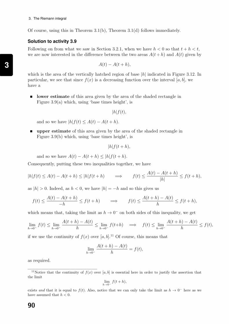
3


Of course, using this in Theorem 3.1(b), Theorem 3.1(d) follows immediately.


Following on from what we saw in Section 3.2.1, when we have h < 0 so that t+ h < t,we are now interested in the difference between the two areas A(t+h) and A(t) given by

A(t)− A(t+ h),

which is the area of the vertically hatched region of base |h| indicated in Figure 3.12. Inparticular, we see that since f(x) is a decreasing function over the interval [a, b], wehave a

lower estimate of this area given by the area of the shaded rectangle inFigure 3.9(a) which, using ‘base times height’, is

|h|f(t),

and so we have |h|f(t) ≤ A(t)− A(t+ h).

upper estimate of this area given by the area of the shaded rectangle inFigure 3.9(b) which, using ‘base times height’, is

|h|f(t+ h),

and so we have A(t)− A(t+ h) ≤ |h|f(t+ h).

Consequently, putting these two inequalities together, we have

|h|f(t) ≤ A(t)−A(t+ h) ≤ |h|f(t+ h) =⇒ f(t) ≤ A(t)− A(t+ h)

|h| ≤ f(t+ h),

as |h| > 0. Indeed, as h < 0, we have |h| = −h and so this gives us

f(t) ≤ A(t)− A(t+ h)

−h ≤ f(t+ h) =⇒ f(t) ≤ A(t+ h)− A(t)

h≤ f(t+ h),

which means that, taking the limit as h→ 0− on both sides of this inequality, we get

limh→0−

f(t) ≤ limh→0−

A(t+ h)− A(t)

h≤ lim

h→0−f(t+h) =⇒ f(t) ≤ lim

h→0−

A(t+ h)− A(t)

h≤ f(t),

if we use the continuity of f(x) over [a, b].11 Of course, this means that

limh→0−

A(t+ h)− A(t)

h= f(t),

as required.

11Notice that the continuity of f(x) over [a, b] is essential here in order to justify the assertion thatthe limit

limh→0−

f(t+ h),

exists and that it is equal to f(t). Also, notice that we can only take the limit as h → 0− here as wehave assumed that h < 0.

90

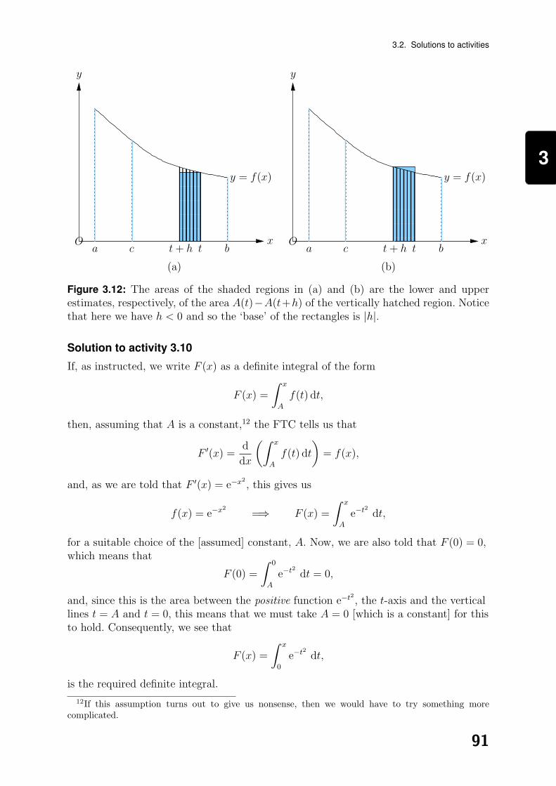
3


��

��

��

��

��

y = f(x)

t+ h

y

xOa bc t ��

��

��

y = f(x)

t+ h

y

xOa bc t

(a) (b)

Figure 3.12: The areas of the shaded regions in (a) and (b) are the lower and upperestimates, respectively, of the area A(t)−A(t+h) of the vertically hatched region. Noticethat here we have h < 0 and so the ‘base’ of the rectangles is |h|.


If, as instructed, we write F (x) as a definite integral of the form

F (x) =

∫ x

A

f(t) dt,

then, assuming that A is a constant,12 the FTC tells us that

F ′(x) =d

dx

(∫ x

A

f(t) dt

)= f(x),

and, as we are told that F ′(x) = e−x2, this gives us

f(x) = e−x2

=⇒ F (x) =

∫ x

A

e−t2

dt,

for a suitable choice of the [assumed] constant, A. Now, we are also told that F (0) = 0,which means that

F (0) =

∫ 0

A

e−t2

dt = 0,

and, since this is the area between the positive function e−t2, the t-axis and the vertical

lines t = A and t = 0, this means that we must take A = 0 [which is a constant] for thisto hold. Consequently, we see that

F (x) =

∫ x

0

e−t2

dt,

is the required definite integral.

12If this assumption turns out to give us nonsense, then we would have to try something morecomplicated.

91

3



Here, we have

F (t) =

∫ t3

4t

x2 dx =

[x3

3

]t34t

=(t3)3

3− (4t)3

3=t9

3− 64

3t3,

and soF ′(t) = 3t8 − 64t2,

in agreement with what we found in Example 3.11.


Firstly, it is easy to verify that we have∫ t

0

1

1 + x2dx =

[tan−1 x

]t0

= tan−1 t− tan−1 0 = tan−1 t,

using the result from Example 5.17 of 174 Calculus and noting that tan−1 0 = 0 becausetan 0 = 0. Then, if a is a constant, we can use this to write

F (t) = tan−1

(a+ t

1− at

)− tan−1 t =

∫ a+t1−at

0

1

1 + x2dx−

∫ t

0

1

1 + x2dx,

so that, using the FTC and its extension as appropriate, we have

F ′(t) =

((1)(1− at)− (a+ t)(−a)

(1− at)2

)(1

1 +(a+t1−at

)2

)− 1

1 + t2,

where we have used the quotient rule to differentiate the upper limit of the firstintegral. Now, considering the first term, we have(

(1)(1− at)− (a+ t)(−a)

(1− at)2

)(1

1 +(a+t1−at

)2

)=

1− at+ a2 + at

(1− at)2 + (a+ t)2

=1 + a2

(1− 2at+ a2t2) + (a2 + 2at+ t2)

=1 + a2

1 + a2t2 + a2 + t2

=1 + a2

(1 + a2)(1 + t2)

=1

1 + t2,

which means that

F ′(t) =1

1 + t2− 1

1 + t2= 0,

as required. But, of course, if F ′(t) = 0, this means that F (t) = c where c is a constantwhich we can find by taking any value of t. So, if we let t = 0, say, we have

c = F (0) = tan−1 a− tan−1 0 = tan−1 a,

92

3

3.2. Exercises

as the value of the constant. Consequently, we have

F (t) = tan−1 a = tan−1

(a+ t

1− at

)− tan−1 t,

which means that, if we rearrange this and let t = b, we have

tan−1 a+ tan−1 b = tan−1

(a+ b

1− ab

),

as required.

Exercises

Exercise 3.1

Consider, for n ∈ N, the partition P = {1, 2, . . . , n} of the interval [1, n]. Find the lowerand upper estimates, L(P) and U(P) respectively, of the integral∫ n

1

1

x(x+ 1)dx,

simplifying your answers as far as possible.

Exercise 3.2

Consider, for n ∈ N, the partition

Pn ={

0, 1n, 2n, . . . , 1

},

of the interval [0, 1]. Find the lower and upper estimates, L(Pn) and U(Pn) respectively,of the integral ∫ 1

0

ex dx,

simplifying your answers as far as possible.

Find limn→∞

L(Pn) and limn→∞

U(Pn). What do these tell us about the value of the integral?

Exercise 3.3

Find f ′(t) when f(t) =

∫ sin t

cos t

x3 dx.

Exercise 3.4

Find the following limits.

(a) limt→0+

t ln t, (b) limt→0+

tt, (c) limt→0+

1

t

∫ t

0

xx dx.

Hence find limt→0+

(ln t)

∫ t

0

xx dx.

93

3


Exercise 3.5

Let f be a continuous function that takes positive real values and suppose that

G(t) =

∫ t2

t

f(x) dx.

Find G′(t) and hence use a Taylor series to find a first-order approximation to G(t) forvalues of t close to 1.

Solutions to exercises


If we sketch the curve y = 1/x(x+ 1) over the interval [1, n] and indicate the points inthe partition P we see that we will be looking at n− 1 rectangles whose bases are givenby the sub-intervals [k − 1, k] for k = 2, 3, . . . , n. Indeed, we see that, for k = 2, 3, . . . , n,each of these sub-intervals gives us a base whose length is

k − (k − 1) = 1,

and so, for the

lower estimate, we need to sum the areas of the n− 1 rectangles illustrated inFigure 3.13(a) where the height of each rectangle is given by the minimum value of1/x(x+ 1) in each of the sub-intervals to get

L(P) = 1

(1

2(2 + 1)

)+ 1

(1

3(3 + 1)

)+ 1

(1

4(4 + 1)

)+ · · ·+ 1

(1

n(n+ 1)

)=

1

2 · 3 +1

3 · 4 +1

4 · 5 + · · ·+ 1

n(n+ 1),

where we have taken each of the sub-intervals in turn and used ‘base times height’to find the area of each rectangle. Then, using partial fractions, we see that

1

k(k + 1)=

1

k− 1

k + 1,

and so we can write

L(P) =

(1

2− 1

3

)+

(1

3− 1

4

)+

(1

4− 1

5

)+ · · ·+

(1

n− 1

n+ 1

)=

1

2− 1

n+ 1,

as the intermediate terms cancel.

upper estimate, we need to sum the areas of the n− 1 rectangles illustrated inFigure 3.13(b) where the height of each rectangle is given by the maximum value of1/x(x+ 1) in each of the sub-intervals to get

U(P) = 1

(1

1(1 + 1)

)+ 1

(1

2(2 + 1)

)+ 1

(1

3(3 + 1)

)+ · · ·+ 1

(1

(n− 1)(n− 1 + 1)

)=

1

1 · 2 +1

2 · 3 +1

3 · 4 + · · ·+ 1

(n− 1)n,

94

3


where we have taken each of the sub-intervals in turn and used ‘base times height’to find the area of each rectangle. Then, using partial fractions again, we can write

U(P) =

(1

1− 1

2

)+

(1

2− 1

3

)+

(1

3− 1

4

)+ · · ·+

(1

n− 1− 1

n

)= 1− 1

n,

as the intermediate terms cancel.

Thus, we have found that the lower and upper estimates of the given integral are

L(P) =1

2− 1

n+ 1and U(P) = 1− 1

n,

respectively.

y =1

x(x+ 1)

y

xO1 2 3 4 nn− 1

...

...

y =1

x(x+ 1)

y

xO1 2 3 4 nn− 1

...

...

(a) (b)

Figure 3.13: The sketches for Exercise 3.1. In (a) and (b) we have, respectively, therectangles that contribute towards the lower estimates, L(P), and the upper estimates,U(P), based on the partition P . Note that, for clarity, the y-intercepts have been omittedand only four of the rectangles are shown.


If we sketch the curve y = ex over the interval [0, 1] and indicate the points in thepartition Pn we see that we will be looking at n rectangles whose bases are given by thesub-intervals

[k−1n, kn

]for k = 1, 2, . . . , n. Indeed, we see that, for k = 1, 2, . . . , n, each of

these sub-intervals give us a base whose length is

k

n− k − 1

n=

1

n,

and so, for the

lower estimate, we need to sum the areas of the n rectangles illustrated inFigure 3.14(a) where the height of each rectangle is given by the minimum value ofex in each of the sub-intervals to get

L(Pn) =1

ne0 +

1

ne1/n + · · ·+ 1

ne(n−1)/n,

95

3



L(Pn) =1

n

(e0 + e1/n + · · ·+ e(n−1)/n

)=

1

n

(1 + e1/n + · · ·+ e(n−1)/n

)=

1

n

(1− (e1/n)n

1− e1/n

)=

1

n

(1− e

1− e1/n

),

where we have used the formula for the sum of a geometric series to get the finalanswer. We now see that writing

limn→∞

L(Pn) = limn→∞

1

n

(1− e

1− e1/n

)= (e−1) lim

n→∞1/n

e1/n−1,

we are dealing with the limit of a quotient where the numerator and thedenominator both tend to zero as n→∞. As such, we can use L’Hopital’s rule tosee that

limn→∞

L(Pn) = (e−1) limn→∞

−1/n2

(−1/n2) e1/n= (e−1) lim

n→∞1

e1/n= e−1,

is the first of the sought after limits.

upper estimate, we need to sum the areas of the n rectangles illustrated inFigure 3.14(b) where the height of each rectangle is given by the maximum value ofex in each of the sub-intervals to get

U(Pn) =1

ne1/n +

1

ne2/n + · · ·+ 1

ne1,


U(Pn) =1

n

(e1/n + e2/n + · · ·+ e1

)=

e1/n

n

(1 + e1/n · · ·+ e(n−1)/n

)=

e1/n

n

(1− (e1/n)n

1− e1/n

)=

e1/n

n

(1− e

1− e1/n

),

where we have used the formula for the sum of a geometric series to get the finalanswer. We now see that writing

limn→∞

U(Pn) = limn→∞

e1/n

n

(1− e

1− e1/n

)= (e−1) lim

n→∞1/n

1− e−1/n,

96

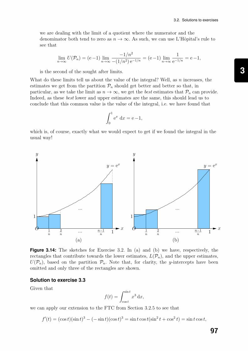
3


we are dealing with the limit of a quotient where the numerator and thedenominator both tend to zero as n→∞. As such, we can use L’Hopital’s rule tosee that

limn→∞

U(Pn) = (e−1) limn→∞

−1/n2

−(1/n2) e−1/n= (e−1) lim

n→∞1

e−1/n= e−1,

is the second of the sought after limits.

What do these limits tell us about the value of the integral? Well, as n increases, theestimates we get from the partition Pn should get better and better so that, inparticular, as we take the limit as n→∞, we get the best estimates that Pn can provide.Indeed, as these best lower and upper estimates are the same, this should lead us toconclude that this common value is the value of the integral, i.e. we have found that∫ 1

0

ex dx = e−1,

which is, of course, exactly what we would expect to get if we found the integral in theusual way!

1n−1n

2n

1

1n

...

...

y = ex

y

xO1n−1

n2n

1

1n

...

...

y = ex

y

xO

(a) (b)

Figure 3.14: The sketches for Exercise 3.2. In (a) and (b) we have, respectively, therectangles that contribute towards the lower estimates, L(Pn), and the upper estimates,U(Pn), based on the partition Pn. Note that, for clarity, the y-intercepts have beenomitted and only three of the rectangles are shown.


Given that

f(t) =

∫ sin t

cos t

x3 dx,

we can apply our extension to the FTC from Section 3.2.5 to see that

f ′(t) = (cos t)(sin t)3 − (− sin t)(cos t)3 = sin t cos t(sin2 t+ cos2 t) = sin t cos t,

97

3


if we use the trigonometric identity sin2 t+ cos2 t = 1.


For (a), we write

limt→0+

t ln t = limt→0+

ln t

1/t,

so that we have a quotient where the numerator and the denominator both tend toinfinity [in magnitude] as t→ 0+. As such, we can use L’Hopital’s rule to see that

limt→0+

t ln t = limt→0+

ln t

1/t= lim

t→0+

1/t

−1/t2= lim

t→0+−t = 0.

For (b), we use the fact that tt = et ln t so that

limt→0+

tt = limt→0+

et ln t = e0 = 1,

if we use our answer from (a).

For (c), we write

limt→0+

1

t

∫ t

0

xx dx = limt→0+

∫ t0xx dx

t,

so that we have a quotient where the numerator and the denominator both tend to zeroas t→ 0+. As such, we can use L’Hopital’s rule and the FTC to see that

limt→0+

1

t

∫ t

0

xx dx = limt→0+

∫ t0xx dx

t= lim

t→0+

tt

1= 1,

if we use our answer from (b).

Then, lastly, we can see that if we use our results from (a) and (c), we have

limt→0+

(ln t)

∫ t

0

xx dx = limt→0+

(t ln t

)(1

t

∫ t

0

xx dx

)= (0)(1) = 0,

as the final answer.


If f is a continuous function that takes positive real values and we are given that

G(t) =

∫ t2

t

f(x) dx,

then, using our extension of the FTC from Section 3.2.5, we find that

G′(t) = (2t)f(t2)− (1)f(t) = 2tf(t2)− f(t).

As such, noting that

G(1) =

∫ 1

1

f(x) dx = 0 and G′(1) = 2(1)f(1)− f(1) = f(1),

we see that a first-order Taylor series about t = 1 gives us

G(t) = G(1) + (t− 1)G′(1) + · · · = 0 + (t− 1)f(1) + · · · = (t− 1)f(1) + · · · ,and so (t− 1)f(1) is the required first-order approximation to G(t) for values of t closeto 1.

98

Documents

Further calculus - University of London · Further calculus A. Ostaszewski, J.M. Ward MT2176, 2790176 2012 Undergraduate study in ... + Ostaszewski, A. Advanced mathematical methods