Embed Size (px)
Citation preview

GraSPP-DP-E-08-003 and ITPU-DP-E-08-001
Funding System and Road Transport;International Comparative Analysis
Katsuhiro Yamaguchi
November 2008
GraSPP Discussion Paper E-08-003 ITPU Discussion Paper E-08-001

GraSPP-DP-E-08-003 and ITPU-DP-E-08-001
Funding System and Road Transport;International Comparative Analysis
Katsuhiro Yamaguchi
November 2008
Professor, Graduate School of Public PolicyThe University of Tokyo
7-3-1, Hongo, Bunkyo-ku, Tokyo, 113-0033, JapanPhone: +81-3-5841-1710
Fax: [email protected]
GraSPP Discussion Papers can be downloaded without charge from: http://www.pp.u-tokyo.ac.jp/
Discussion Papers are a series of manuscripts in their draft form. They are not intended for circulation or distribution except as indicated by the author. For that reason
Discussion Papers may not be reproduced or distributed without the written consent of the author.

Funding System and Road Transport; International Comparative Analysis
Katsuhiro Yamaguchi1 Graduate School of Public Policy, The University of Tokyo, Japan
Abstract
Tension between necessity for infrastructure investment and scarcity of public capital is inevitable in modern motorized nations. When fiscal policy needs to be tightened public investment may face deceleration. On the other hand lax funding scheme may give way to over-investment. After an overview of recent trend in funding system of road investment this paper highlights institutional differences in five major nations, USA, UK, France, Germany and Japan, and examines how actual investment is affected. Between 1990 and 2004, we find that in nations such as USA and Japan, where road fund is established, the level of hypothecated fuel tax revenue affects road investment while in other three nations such a relationship is not observed. In USA, Germany and Japan general fiscal condition of the government, indexed by primary balance, has significant effect on road investment with time lags ranging from 1.5 to 4.6 years. In UK and France there is no evidence of such an effect.
Given the funding system, we then assess efficiency of road transport in these five nations during the same period from two perspectives; efficiency in terms of 1) how road network has impacted macro-economic MFP growth and 2) how the road transport system as a whole is performing. For the former, this paper reveals that impact of road capital improvement on macro-economic MFP growth is positive only to the extent that physical network had expanded. In Japan and USA and more recently in Germany disproportionate growth in nominal value of road capital has negatively affected MFP growth. For the latter, road transport system composed of road network, automobiles and fuel consumption has been improving with the exception of Japan. Redundancy of transport networks and sparse land-use are major sources of inefficiency.
Keywords: Funding system, road investment, MFP, efficiency.
1 Tel. : +81-3-5841-1710; fax : +81-3-5841-7877 E-mail address: [email protected] (K. Yamaguchi)

1. Introduction 20th Century could be characterized as an era of automobiles. Faced with
motorization each nation has aligned its funding system to cope with development of necessary infrastructure. Evolution of funding system depends not only on genuine need for infrastructure, but also on public policy framework and political manifestation.
For infrastructure authorities the way in which the funding system is structured is a major concern. There are a number of key institutional factors that shape the scheme. First is the institutional difference in government fund and taxation. Some nations have special fund dedicated to road investment while some do not. Some special funds cover transit as well as roads while some only deal with the latter. Taxation of automobile ownership and usage has become one of major ways to raise government revenue. Some are pooled to the special fund while some are sourced to the general government account. Reasons of taxation may differ accordingly. When a special fund is formed, pressure from the treasury is often alleviated and the government institution in charge of infrastructure attains more power. Such a scheme is attractive for infrastructure authorities while the other side of the coin is that for the treasury flexibility of cross sectoral funding is reduced.
Second is the extent to which concession is used. In most nations, infrastructure such as turn-pikes, highways, bridges and tunnels have been more or less financed by such a vehicle. Mega-projects that require large lump-sum capital up-front are often spun-off to concessions that finance through government secured bonds. In some major concessions, actual traffic is way below the estimate, resulting in poor return on investment. Risk of inefficient investment is always a concern for the tax payers. Private capital involvement has thus become increasingly common in securing Value for Money.
Third, government facing financial difficulty does not only look for expenditures to cut but also assets to sell. Today, transport infrastructures are on the table list of many governments in need of fiscal reform. Privatization of governmental concessions and leasing out toll roads could tighten the tap as well as provide ways for governments to clean the balance sheet.
In sum, tension between need for infrastructure investment and scarcity of capital resource is inevitable in modern motorized nations. When the fiscal policy needs to be tightened deceleration of infrastructure improvement may occur, resulting in lower potential economic growth. Soft funding scheme, on the other hand, may give way to over-investment.
Another major concern for the infrastructure authorities is the efficiency of
investment. How would difference in funding system affect the performance of road investment? What difference would it make to the productivity and efficiency of the national economy and the road transport system?
Since 1990’s there has been an outburst of analysis regarding macro-economic productivity of public investment. Pioneering work by Aschauer (1989) attributed poor economic performance to the deteriorating public infrastructure. Although a number of subsequent studies2 contended that empirical evidence of its contribution is at best fragile, recent analysis on road investment tends to yielded positive effects. Fernald (1999) identified relatively high causal relationship between road investment and productivity growth in industries with high automobile intensity in USA. Kopp (2007) confirms similar effects in Europe. Nakazato (2005) applied growth regression approach on highway investment in Japan through 1960 to 1999 and reported positive effects until 1970’s after which it has diminished. Another area of interest is the efficiency of the road transport system as a whole. Various productivity measurement methodologies have been applied to transport infrastructure such as airports, sea ports and railways. Roads, however, has not been the object of analysis. Efficiency of road transport depends not only on infrastructure but also on automobile and its usage. At the national level, it may also be affected by the level of other transport modes and urbanization.
This paper tries to highlight some of these contemporary issues in road investment and road transport system. In particular we take a close look at road investment in five major nations; USA, UK, France, Germany and Japan. Empirical analyses focus on period between 1990 and 2004 to identify the impacts of recent policy changes in road investment.
The rest of the paper is organized as follows. Next section gives a short description of the evolution of funding system for road investment. Funding systems in the five nations are elaborated. In section three, effect of the funding system on road investment is analyzed. Quantitative analysis of how road investment is affected by revenue level of special fund and the general condition of the treasury is presented. In section four, we conduct a regression analysis to identify road investment’s impact on macro-economic multi factor productivity growth (MFP) and argue that physical improvement of the road capital stock has positive effect while nominal monetary value of the stock causes distortion in productivity assessment. Section five utilizes a number of methodologies to assess efficiency of road transport systems and identify factors behind the discrepancy between the five nations. Section six gives concluding remarks. 2 See for instance Holtz-Eakin (1994) and Strum (1998).

2. Evolution of funding system for road investment 2.1 General trend
Pre-automobile history of road network developed in two different ways. One was the authentic construction by the public sector. Urban road networks were usually under the responsibility of local governments. Two was the turnpikes. These long route structures, often developed by trusts and semi-private enterprises, were tolled to cover maintenance cost and in some instances to finance new construction. Advent of railway in the 19th century caused most turnpikes to be consolidated. In the 20th century road construction entered a new era with the rise of the automobiles. Need for dramatic improvement of the network was accelerated by national defense objectives. The sheer size of the investment and the difficulty of collecting user-charges lead governments to engage themselves directly in trunk route development. As government’s role grew in various functions scarcity of public capital became severe. Fuel and automobile ownership became one of major objects of taxation.
Fiscal policy needs the flexibility of resource allocation in response to changes in policy agenda. Infrastructure development, on the other hand, requires a stable fund. In UK, France, USA and then in Japan special government funds or accounts were established to hypothecate automobile related tax for road expenditure. Some of the mineral oil tax in Germany was also earmarked to road investment absent a special fund. As witnessed in abolition of the UK Road Fund in 1995, and also in subsequent history in France with Le Fonds Special d’Investissement Routier (FSIR) established in 1951 and ceased in 1981, special fund is neither universal nor eternal. In Germany portion of the fuel tax and the recent introduced autobahn charge on large commercial vehicles (HGV) are dedicated in part to road investment but less than a quarter of total motor-transport levies is appropriated to expenditure on roads3. Characteristics of the funding system and the level of automobile related tax are illustrated in Figure 1 and Figure 2.
(Figure 1 and Figure 2 about here) “Pay as you go“ has been the common principle in many governments. In order
to circumvent the pay-go rule public agency with a special purpose of financing and constructing infrastructure was often established. These agencies issued bonds backed by the government to raise funds. Since they cannot rely on taxation as a revenue stream 3 VDA (2007)

tolling was used to pay back the loans. Future projection of road transport demand was often tempted to be overestimated resulting in lack of credible investments. The idea of PFI/ PPP is to involve the private sector that is more parsimonious and better at project management. There has been repercussion, however, after the initial offspring of PFI/PPP projects. Potential benefits and limitations are still to be judged.
In the following section, a brief history of road investment funding systems in five major nations, USA, UK, France, Germany and Japan, is introduced. Table 1 underpins the basic characteristics of these five nations.
(Table 1 about here) 2.2 Funding system in major nations 2.2.1 USA
Highway Account of Highway Trust Fund was established in 1956 to pool fuel tax revenue for financing transport infrastructure investments including federal inter-state highways. Basic rule was that capital outlay for a given fiscal year would be limited to the resources available to the states in that year. Also, tolling was prohibited on interstates. In the 1960’s mass transit was added to its responsibility. Under ISTEA (1991-97) tolling on non-Interstates was made possible and under TEA-21 (1998-2003) three new financial tools were introduced; State Infrastructure Banks (SIB), Transportation Infrastructure Finance and Innovation Act (TIFIA) credit assistance and Grant Anticipation Revenue Vehicles (GARVEEs). Also, conversion of free highways into tolled roads has been made possible. Under the current SAFETEA-LU (2005- ) a number of tolling-related programs are continued and initiated. Concession is not only used for new constructions. In recent years local governments have started to pursue the concession model for existing infrastructures. Chicago Skyway and Indiana Toll Roads are recent examples of take-over of existing structure by long-term concessions. 2.2.2 UK
Turnpikes that were developed before the advent of railways and automobiles were consolidated by the public sector in the early 20th century. Road Fund established in 1909 pooled fuel tax subsequently converted into registration fees. Earmarking, however, was generally loose. In the 1960’s and 70’s central support to the local governments were reinforced by Rate Support Grant and Transport Supplementary Grant. Since the 1980’s a series of fiscal consolidation did not leave road infrastructure without change. Road Fund was terminated in 1995. PFI application on road was promoted through Design-Build-Finance-Operate (DBFO). According to the UK Highway Agency the estimated total capital value of the road schemes within the DBFO

highway program is close to £1.3 billion. Another distinct feature is the integrated transport policy orientation. Since the late 1990’s transport policy has placed strong emphasis on sustainable transport through railway reform, transport-land-use planning, road-user charge, etc. Congestion pricing introduced in London as of 2003 is a milestone in contemporary urban transport policy. 2.2.3 France
In France road was considered as strategic infrastructure by the reigns since the pre-automobile era. Heritage was as much as 40,000 km by 1930. Initially 22% of fuel tax was appropriated to FSIR, a special fund for road investment established in 1951. As the government deficit accumulated, more and more resources were diverted to the general account and FSIR was eventually terminated in 1981. Loi d’Orientation des Transports Interierus (LOTI) enacted in 1982, promoted decentralization of government agencies and utilization of private initiatives. Semi-public corporations, Societe d’Economie Mixte, in charge of motorways were established. During 1982 – 86 Special fund for mega-projects, Le Fond Special de Grands Travaux, funded large investments in road, public transport and energy saving projects. The fund depended on increased fuel tax, but as for roads, general funds were reduced so that the total expenditure did not experience significant increase. Since 1990 a fund for the capital city of Paris, le Fond pour l’Amenagement de l’lle de Franc, is serving social infrastructure investments. In 2004 Agence de Financement des Infrastructures de Transport de Franc was established to invest in mega-projects. 2.2.4 Germany
Roads in Germany have historically been developed without tolls. Until levy on trucks over 12 metric tons (HGV) was introduced in 2005 the highway system, Bundesautobahn, had been developed as 12,000km of toll-free system. In addition to general government fund, mineral oil tax, incremental portion of which pooled for transport infrastructure since 1955, has been the major source of road investment. German transport policy has a strong emphasis on railway and the mineral oil tax revenue has been utilized for trunk and transit railroads. Since reunification need for transport infrastructure investment was accelerated. EU fiscal policy on government deficit has put a cap on public spending. In 1994 legislation was passed to allow BOT concession for bridges and tunnels. However, only two of these projects are operational as of 2007. Introduction of HGV toll has opened a window of opportunity for PPP in trunk roads. Verkehrsinfrastrukturfinanzierungsgesellschaft (VIFG), a state owned agencey established in 2003, is supporting lane-expansion projects funded by HGV toll revenue. First of these A-model projects was awarded by VIFG in 2007.

2.2.5 Japan In Japan a series of fuel tax was introduced in the 1950’s and pooled into the
Road Improvement Special Account (RISA), established in 1958. Additional tax on ownership of automobile was introduced in 1971. Quarter of the revenue was distributed to local governments for road expenditure and 80% of the rest was apportioned to the RISA through the general account. Roads are classified into national, prefecture and local roads. Tax level was increased to match the five year investment plan. Abundant resource in RISA sometimes cause overflow. Public transport is outside the scope of RISA4. Basic rule under the legislation is that usage of roads must be free of charge except for tolled roads5. The enterprise tasked to develop nation-wide highway, Japan Highway Public Corporation (JH) established in 1956, was a public corporation which raised most of its capital through government backed loans payable by future toll revenue6. Since 1985, when Japanese economy embarked on a mission to turn the export-oriented economy into a system that depended more on endogenous growth, the level of public investment was lifted. During the economic turmoil in the 1990’s, additional fund from the general account was poured into new road construction to counter recession. With only 1/25 the size and half the population, road investment in Japan had exceeded that of US during the 1990’s. Since the turn of the century, the prime-ministership has put an end to the soft budget. After a political vanquish, JH, a powerful entity in highway development, was privatized into one highway holding company and three regional highway corporations in 2005. In 2008 five special funds on public investment including RISA are planned to be integrated. 3. Effect of the Funding System on Road Investment
In this section we investigate how the funding system affects road investment. In nations with specific fund institution the level of road investment is expected to be influenced by the level of revenue. There may be a time lag due to account settlement, although it is expected to be short. Another factor affecting road investment is the general condition of the fiscal policy. Using panel data fro 22 OECD countries for the period 1980-92 Strum (1998) found that government capital spending is reduced during fiscal stringency. We test the hypothesis with primary balance. When primary balance is 4 Treasury has been eyeing on RDSA funds to expend for general purposes. This, of course, is faced by opposition from the construction and automobile industry backed by politicians. Some argue that at least reimbursement of the government debts incurred for road investment should be born by the automobile users. 5 Toll road needs to be turned into free road once debt service is completed. 6 There are a number of toll rods operated by local public agencies as well as a small number of private turnpikes which are regulated as a business enterprise.

negative and increasing necessity to restore the situation tightens government budget for capital outlay. This effect, if it exists, is expected to yield time lag since adjustment by the treasury often involves political decision making which takes time. Figures 3-1 to Figure 3-3 illustrate recent trends of relevant data in USA, UK, France, Germany and Japan.
(Figures 3-1, 3-2 and 3-2 about here) We analyze these two effects through level of fuel taxation revenue7 (REV)
which is the major source of road investment and primary balance (PB) both in terms of share in GDP and standardized. Gross road investment in percentage share of GDP (RI) is regressed against these variables with lags8. The result is depicted in Table 2.
(Table 2 about here) In both USA and Japan, where special fund is institutionalized, fuel tax revenue
has positive and statistically significant effect on road investment. Average time lags are 2.3 years and 1.0 year respectively. As for primary balance USA, Germany and Japan have positive and significant effect on road investment. Average time lags are 4.6 years, 3.3 years and 1.5 years respectively. Neither fuel tax revenue nor primary balance is affecting road investment in UK and France. 4. Road investment and Economic Growth
Efficiency of transport infrastructures has a number of different perspectives. Here we are concerned with the economic impact of infrastructure investment on macro economic performance. We are interested in identifying how public capital stock, along with labor and private capital stock, enters into the macro production function and affects productivity growth of an economy as a whole.
We use a simplified version of specification presented by Fernald (1999) and extended by Kopp (2007). National economy could be modeled as follows:
),,( iiii
ii GLKFUY =
7 For USA and Japan vehicle tax revenue is included. 8 Almon lag is used for time lag specification.

where, iY is output, iU is Hicks-neutral technology level, )(JF i is production
function with three arguments; iK as private capital, iL as labor and iG as road
capital of country i . Cost minimization implies that elasticity of each input equals
input’s share Jis . Thus Solow’s MFP growth residual idp could be expressed by
growth rate of inputs, as follows:
iGiiLiiKiii dgsdlsdksdydp −−−≡
Let idu be the technology improvement. Then the above equation could be rewritten
as follows:
iiGii dudgsdp += φ
We estimate the following regression model with panel data of five nations, USA, UK, France, Germany and Japan for years between 1992 and 2004, thus transcript t is added.
ittiitGititit dpdgscdp εφ +++= −1,
itdu is represented by the constant term itc . 1, −tidp is the lagged variable. itε .is the
error term. Data sources are listed in the Appendix. All monetary figures are converted into PPP adjusted international constant9 US Dollars. Hausman specification test with respect to the fixed effect model supported random effect model. GMM is also run to enhance robustness. (Table 3-1 and Table 3-2 about here)
Result of the panel regression is listed in Table 3-1 and GMM in Table 3-2. Three different data are used for road investment. First, road capital growth in physical unit (kilometers) is used. Coefficient is 0.1782. The order is in line with previous studies. Next we used nominal road capital value. The coefficient is negative so we adjust the value by deflator calculated by setting nominal road capital value per kilometer in year 2000 as 100.
9 Constant at year 2000.

(Figure 4 about here) From Figure 4 we can see that Japan and to a less extent USA have experienced
“inflation.” Adding an incremental kilometer of road has become more and more expensive. It has pushed up the nominal road capital value such that its effect on MFP growth is negative. The third row indicates the result of the regression analysis using the deflated value. Coefficient of road capital value growth is 0.1847, a similar value to that of road capital growth in physical unit. This implies that MFP growth responds to the physical improvement of the road network and not to the nominal capital value invested. GMM yields slightly lower coefficients but they are statistically significant.
5. Efficiency of Road Transport We now focus on the efficiency of the road transport sector. Road transport as a
service could be expressed in the form of a production function. Ingram and Zhi (1999) take the production function approach but take the number of motor vehicles per kilometer of road as a proxy of input ratio. Here, we take the direct approach in measuring productivity. Productivity, the ratio of output and input, could be calculated relatively simply if there is only one output and input. If we have multiple outputs and/or inputs, however, we need to aggregate these multiple factors into an index to derive the ratio. In this section we consider a case with one output; vehicle kilometer performed, and three inputs; road, automobile and fuel.
The following three methodologies are used to derive efficiency indices. Econometric production function model assumes that each country’s road transport system is efficient. This assumption is unlikely to hold so DEA and Tornqvist index are also deployed. It is followed by an analysis of multilateral superlative Tornqvist index to compare efficiency change among the five countries and identify factors that explain the difference10.
1) Production function model 2) Data envelopment analysis (DEA) 3) Tornqvist index
5.1 Production function model
Production function model has an advantage in that parametric estimation of a
10 Another efficiency measurement methodology, stochastic frontier, is used to check the results from multilateral superlative Tornqvist index analysis.

production function form could be conducted and statistically verified. The other side of the coin is that specification of a production function is necessary. With respect to the estimated efficiency level, trend of each observation over time could be identified.
Methodology using constant rate of substitution (CRS) production function proposed by Yoshida (2005) is modified to Cobb=Douglas production function specification. Following equation was estimated using panel data 2SLS fixed effect model11.
ittitiitititit uvvkmautofuelroadcvkm +++++++= − μαααα 1,4321 lnlnlnln
where,
itvkmln : natural log of vehicle kilometers performed (standardized values) in country i
in year t.
1,ln −tivkm : lag (1) value of itvkmln
itroadln : natural log of total road length (standardized) in country i in year t.
itfuelln : natural log of total fuel consumed (standardized) in country i in year t.
itautoln : natural log of total number of automobiles in use (standardized) in country i
in year t. c : time invariant constant term across all observations
iμ : time invariant fixed effect for country i
tv : dummy variable for year t
itu : error term
Productivity )ˆexp(ln/)exp(ln ititit mkvvkme =
Productivity growth is derived by;
titi ee ,1, /+
11 Natural log of number of automobiles, fuel price, GDP, population (standardized values).

itmkv ˆln : estimated value of itvkmln from the above equation.
Result of the estimate for the production function is listed on Table 4. As expected, coefficients of total road length and fuel consumption are positive and statistically significant. Result of the second equation shows that coefficient of number of automobiles is not statistical significance. This could be explained by the supplemental nature of automobiles to road infrastructure. Productivity growth is depicted together with results of other methodologies in Figure 5-1 to 5-5. Although there is a general tendency of positive growth, fluctuation makes it difficult to infer specific conclusion.
(Table 4, Figures 5-1 to 5-5 about here)
5.2 Data Envelopment Analysis Data envelopment analysis (DEA) measures efficiency by distance function
relative to production possibility curve using linear-programming techniques. It is a flexible approach in that production possibility curve is derived from non-parametric methods without specifying a functional form and also without input price data. Its disadvantage is that the derivation of production possibility curve is affected by outliers. Malmquist index given as follows by Coelli et al (2005) is frequently used for productivity comparison between two time periods s and t.
2/1]),(),(
),(),(
[),,,(ss
to
ttto
ssso
ttso
ttsso xqdxqd
xqdxqd
xqxqm ×= ,
where, ),( λλλ xqdo is the distance of pair of output and input vectors ),( λλ xq with
respect to production possibility curve by technology λ =s, t. Malmquist index is computed by DEAP Version 2.1 provided by Coelli, T.J.
Again, the result of the productivity growth measurement is depicted together with results of other methodologies in Figure 5-1 to 5-5. DEA Malmquist index is in parallel form and slightly exceeding that of the production function model. 5.3 Tornqvist Index
TFP growth expressed as Tornqvist index is defined as follows:

it
ti
it
ti
it
ti
XX
YY
TFPTFP 1,1,1, lnlnln +++ −= , where itY : output, itX : input
For inputs we consider road GitX , automobile A
itX and fuel FitX , with G
its , Aits and
Fits as cost share of road, automobile and fuel respectively. The equation then becomes;
Fit
FtiF
itFtiA
it
AtiA
itAtiG
it
GtiG
itG
tiit
ti
it
ti
XX
ssX
Xss
XXss
YY
TFPTFP 1,
1,1,
1,1.
1,1,1, ln)(
21ln)(
21ln)(
21lnln +
++
++
+++ +−+−+−=
As illustrated by Figure 5-1 to Figure 5-5 the three different methodologies of efficiency measures yield similar results. Since these indices are not comparable across nations, we calculate the superlative index to observe difference between them. 5.4 Multilateral superlative Tornqvist Index
Multilateral superlative Tornqvist index developed by Caves, Christensen and Diewert (1982) could be applied to the road transport system as follows:
Let tY)
be geometric mean of tY , tY be arithmetic mean of tY , and similarly for
ktX) k
tX kts) k
ts where k=G, A, F.
Then, with average level of output and inputs in year one as the benchmark, multilateral superlative Tornqvist index growth for country i in year t would be as follows:
Ft
FtiF
tFtiA
t
AtiA
tAtiG
t
GtiG
tG
tit
ti
it
ti
XX
ssX
Xss
XX
ssY
YTFP
TFP))))
1,1,
1,1,
1,1,
1,1, ln)(21ln)(
21ln)(
21lnln +
++
++
+++ +−+−+−=
]ln)(21ln)(
21ln)(
21ln[ 1
11
11
11
1
1Fs
FsF
sFsA
s
AsA
sA
sGs
GsG
sGs
s
st
s XX
ssXX
ssXX
ssY
Y)
)
)
)
)
)
)
)+
++
++
++
−
=
+−+−+−+∑
Multilateral superlative Tornqvist index plotted in Figure 6 shows that UK and USA followed by Germany and France are efficient and Japan is in a dismally poor position. Stochastic frontier analysis yields similar results12. Here again efficiency in Japan lags behind others.
12 Stochastic frontier analysis was conducted by open program FRONTIER ver. 4.1 provided by Coelli, T.J. One output (vehicle kilometers) and three inputs (road length, number of automobiles and fuel consumed) are used.

(Figure 6 and Table 5 about here) In order to identify factors behind the difference, multilateral superlative
Tornqvist index was regressed against the following seven variables; highway length
per land area ( ithighway ), ratio of new automobile sales to the stock of vehicles
( itnewauto ), Population density ( itpop ), urban population ratio ( iturban ), annual
change in percentage of population aged over 65 ( itover65 ), railway length per land
area ( itrail )and internet users per population ( iternetint ).
The first two variables try to capture the technical improvement in road infrastructure and automobiles. Positive effects would be expected if there are technical improvements in infrastructure by enhanced throughput of vehicles. Also, speed improvement, fuel efficiency etc. in automobiles could increase the total efficiency of the road transport system. Population density reflects the level of congestion, thus it is expected to have a negative coefficient. Aging society makes society more immobile so it is expected to have a negative effect on efficiency. Higher railway intensity is expected to result in lower efficiency of road transport since the redundancy is higher. Level of urbanization is expected to have a positive coefficient since the road transport assets are used more intensively. Higher internet usage may have a negative effect on toad transport efficiency if its substituting effect overrides the spillover effect of enhanced communication on spatial activities.
In Table 5 result of the panel regression is listed. Hausman test supported the fixed effect model. The first two variables turned out to be insignificant, meaning that technical improvement in road infrastructure and automobiles does not affect the efficiency of the road system. The other variables were statistically significant at the 1%
or the 5% level. As expected, itpop , itover65 and itrail have negative effect on
efficiency of road transport while iturban and iternetint have positive impacts.
6. Concluding Remarks

Tension between necessity for infrastructure investment and scarcity of capital resource is inevitable in modern motorized nations. When the fiscal policy is consolidated lack of investment in infrastructure may lead to deceleration of economic growth. On the other side lax funding scheme may give way to over-investment. After an overview of recent trend in funding system of road investment this paper identified institutional differences in five major nations, USA, UK, France, Germany and Japan. In nations such as USA and Japan, where special fund is established, the level of fuel tax that is hypothecated to road investment affects the level of road investment. Other three nations do not exhibit such relationship. In USA, Germany and Japan general fiscal condition of the government, indexed by the level of primary balance, has significant effect on road investment with time lags ranging from 1.5 to 4.6 years.
Impact of road capital improvement on macro-economic productivity growth is positive only to the extent that physical network had expanded. Japan and USA in the 1990’s and more recently in Germany have experienced excessive growth in nominal value of road capital affecting negatively on MFP growth. In the five nations, road transport system composed of road capital, automobiles and fuel consumption has been improving with the exception of Japan in which multilateral superlative Tornqvist index is lagging far behind other four nations. Redundancy of transport network with other transport mode such as railway and sparse land-use are some of the major sources of inefficiency.
In sum, funding system could make a difference in road investment. It is not, however, a sufficient condition. General fiscal consolidation may or may not affect road investment. Earmarking may provide stable resources but could lead to inefficient investment in the sense that contribution to macro-economic productivity growth is watered down by costly capital outlay per incremental increase in physical road asset. Efficiency of the transport system as a whole may also be affected. In order to realize an efficient road transport system integrated transport policy with multi-modal and transport/land-use consideration should be pursued.

Reference Aschauer, David A., 1989. Is public expenditure productive? Journal of Monetary
Economics, 23, 177-200. Caves, D.W., Chiristensen, L.R., Diewert, W.E., 1982, The economic theory of index
numbers and the measurement of input, output and productivity, The Economic Journal, 92, 73-86.
Coelli, T.J., Prasada Rao, D.S., O’Donnell, C.J., Battese, G.E., 2005. An introduction to efficiency and productivity analysis, second edition. Springer, New York.
Fraumeni, B.M., 1999, Productive Highway Capital Stock Measures, Federal Highway Administration, US Department of Transportation
Fernald, J.G., 1999, Road to prosperity? Assessing the link between public capital and productivity, American Economic Review, 89, 619-638.
Holtz-Eakin, D., Schwartz, A.E., 1995, Infrastructure in a structural model of economic growth. Regional Science and Urban Economics 25, 131-151.
Ingram, G.K., Zhi, L., 1999, Determination of motorization and road provision, in Essays in transportation economics and policy, Brookings Institution Press, Washington D.C.
Kopp, A., 2007, Macroeconomic productivity effects of road investment, in Transport Infrastructure Investment and Productivity, OECD/ECMT, Paris.
Nakazato, T., 2005, Kosokudoroseibi no genjo to kadai (Current situations and issues in highway development), in Kokyobumon no gyouseki hyouka, The University of Tokyo Press, Tokyo (in Japanese).
Strum, J., 1998. Public Capital Expenditure in OECD Countries. Edward Elgar, Cheltenham, UK.
Verband der Automobilindustrie (VDA), 2007, Annual Report 2007. Vickerman, R., 2005, Infrastructure Policy, in Handbook of Transport Strategy, Policy
and Institutions, 225-235, Elsevier, Amsterdam. Yoshida, Y., 2004. Endogenous-weight FP measurement: methodology and its
application to Japanese-airport benchmarking. Transportation Research: Part E 40 (2), 151-182.
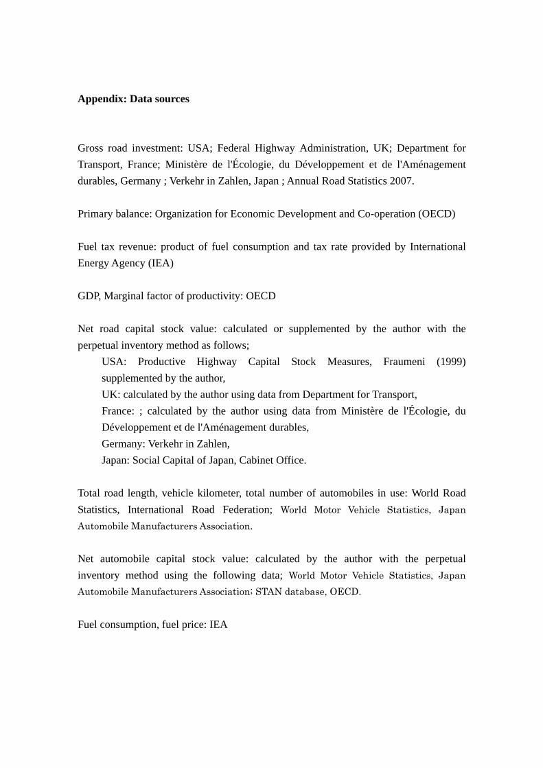
Appendix: Data sources Gross road investment: USA; Federal Highway Administration, UK; Department for Transport, France; Ministère de l'Écologie, du Développement et de l'Aménagement durables, Germany ; Verkehr in Zahlen, Japan ; Annual Road Statistics 2007. Primary balance: Organization for Economic Development and Co-operation (OECD) Fuel tax revenue: product of fuel consumption and tax rate provided by International Energy Agency (IEA) GDP, Marginal factor of productivity: OECD Net road capital stock value: calculated or supplemented by the author with the perpetual inventory method as follows;
USA: Productive Highway Capital Stock Measures, Fraumeni (1999) supplemented by the author, UK: calculated by the author using data from Department for Transport, France: ; calculated by the author using data from Ministère de l'Écologie, du Développement et de l'Aménagement durables, Germany: Verkehr in Zahlen, Japan: Social Capital of Japan, Cabinet Office.
Total road length, vehicle kilometer, total number of automobiles in use: World Road Statistics, International Road Federation; World Motor Vehicle Statistics, Japan Automobile Manufacturers Association. Net automobile capital stock value: calculated by the author with the perpetual inventory method using the following data; World Motor Vehicle Statistics, Japan Automobile Manufacturers Association; STAN database, OECD. Fuel consumption, fuel price: IEA

Figure 1: Characteristics of funding system for road investment in the five nations
Figure 2: Level of annual automobile related tax (2004)
0
500
1000
1500
2000
2500
USA UK France Germany Japan
Vehicle tax
Fuel tax
** **
***: source of special fund for road investment: appropriated for road investment
US$
Source: Annals of Road Statistics (2006) MLIT, Japan, converted by PPP exchange rate (2004)Annual automobile tax burden estimated with a standard automobile weighing 1.5 tons, 6-year vintage, annual fuel consumption of 1,200 liters. Tax rate as of Jan. 2005.
Special funds or accounts
General funds
Taxation on automobile ownership and usage
Japan*
USA
UK
GermanyFrance*
*relatively receptive to highway concessions

0
0.005
0.01
0.015
0.02
0.025
1990
1992
1994
1996
1998
2000
2002
2004
USA
UK
France
Germany
Japan
Figure 3-1: Gross road investment’s share of GDP
0
0.005
0.01
0.015
0.02
0.025
0.03
0.035
1990
1992
1994
1996
1998
2000
2002
2004
USA
UK
France
Germany
Japan
Figure 3-2: Fuel tax revenue’s share of GDP
-0.08
-0.06
-0.04
-0.02
0
0.02
0.04
0.06
0.08
1990
1992
1994
1996
1998
2000
2002
2004
USA
UK
France
Germany
Japan
Figure 3-3: Primary balance’s share of GDP

Road capital value deflator (2000=100)
0
20
40
60
80
100
120
140
1990
1992
1994
1996
1998
2000
2002
2004
USA
UK
France
Germany
Japan
Figure 4: Road capital value deflator (2000=100)

Figure 5-1: Road transport TFP change in USA
Figure 5-2: Road transport TFP change in UK
-0.04
-0.03
-0.02
-0.01
0
0.01
0.02
0.03
1992
1993
1994
1995
1996
1997
1998
1999
2000
2001
2002
2003
2004
Productionfunction
DEA
Tornqvist
-0.08
-0.06
-0.04
-0.02
0
0.02
0.04
0.06
1992
1993
1994
1995
1996
1997
1998
1999
2000
2001
2002
2003
2004
Productionfunction
DEA
Tornqvist

Figure 5-3: Road transport TFP change in France
Figure 5-4: Road transport TFP change in Germany
-0.04
-0.03
-0.02
-0.01
0
0.01
0.02
0.03
0.04
0.05
1992
1993
1994
1995
1996
1997
1998
1999
2000
2001
2002
2003
2004
Productionfuncetion
DEA
Tornqvist
-0.06
-0.04
-0.02
0
0.02
0.04
0.06
0.08
0.1
1992
1993
1994
1995
1996
1997
1998
1999
2000
2001
2002
2003
2004
Productionfunction
DEA
Tornqvist

Figure 5-5: Road transport TFP change in Japan
-0.04
-0.03
-0.02
-0.01
0
0.01
0.02
0.03
1992
1993
1994
1995
1996
1997
1998
1999
2000
2001
2002
2003
2004
Productionfunction
DEA
Tornqvist

Figure 6: Multilateral superlative TFP index
-0.25
-0.2
-0.15
-0.1
-0.05
0
0.05
0.1
0.15
0.2
1992
1993
1994
1995
1996
1997
1998
1999
2000
2001
2002
2003
2004
USA
UK
France
Germany
Japan

Table 1: Summary of statistics for the five nations
Total
road
length*
Number
of
automob
iles*†
Annual
fuel
consumpt
ion**††
Populat
ion* GDP**
Land
size
Inhabita
ble land
Annual
road
investm
ent**
Annual
road
mainten
ance**
Annual
road
expendit
ure**
Annual road
investment
per GDP**
Annual
road
maintenan
ce per
GDP**
Annual
road
expenditur
e per
GDP**
thousand
km million
billion
liters million
billion
US$
1000
km2
1000
km2
billion
US$
billion
US$
billion
US$ - - -
USA 6,408 243 653 294 10,574 9,629 6,199 64 33 97 0.61% 0.31% 0.92%
UK 388 34 51 60 1,722 243 217 4 6 10 0.23% 0.35% 0.58%
France 1,002 36 55 60 1,645 552 400 11 5 16 0.67% 0.30% 0.97%
Germany 657 49 68 83 2,191 357 242 18 3 21 0.82% 0.14% 0.96%
Japan 1,188 75 98 128 3,456 378 118 55 16 71 1.59% 0.46% 2.05%
Note: * as of Jan 1st 2004, ** year of 2004, Monetary figures are in PPP exchange rate converted 2000 constant US Dollars. See Appendix for data sources. †Cars, buses and trucks †† Automobile fuel including gasoline, diesel and LPG are converted into unleaded gasoline equivalent units ††† tax on automobile ownership and usage hypothecated to special fund on road investment.

Table 2: Results for regression analysis of gross road investment and fiscal conditions
Dep.var.=RI C REV REV(-1) REV(-2) REV(-3) REV(-4) REV(-5) PB PB(-1) PB(-2) PB(-3) PB(-4) PB(-5) RHO Ad. R2
USA Estimate -0.002 0.039 0.294 0.312 0.208 0.099 0.103 -0.00003 0.00006 0.00003 -0.00003 -0.00002 0.00016 -0.969 0.995
t-statistics -3.956 1.723 18.048 22.968 8.437 2.898 3.261 -17.865 18.239 14.221 -13.267 -4.896 45.961 -22.218
p-value [.000] [.085] [.000] [.000] [.000] [.004] [.001] [.000] [.000] [.000] [.000] [.000] [.000] [.000]
sum of lag 1.055 [14.480] 0.00017 [63.940]
average lag 2.326 4.561
UK Estimate 0.014 -0.131 -0.096 0.012 0.085 0.018 -0.294 0.00001 -0.00005 -0.00004 0.00001 0.00004 0.00000 -0.965 0.988
t-statistics 3.657 -8.459 -1.744 0.253 4.965 1.557 -12.867 0.327 -1.482 -1.298 0.499 5.847 -0.134 -19.480
p-value [.000] [.000] [.081] [.800] [.000] [.120] [.000] [.744] [.138] [.194] [.618] [.000] [.893] [.000]
sum of lag -0.406 [-2.905] -0.00004 [-0.3368]
average lag 2.996 -0.948
France Estimate -0.094 0.701 -0.784 -0.230 1.070 1.823 0.735 0.00008 -0.00107 -0.00140 -0.00103 -0.00009 0.00130 -0.890 0.982
t-statistics -1.632 4.855 -1.850 -2.153 1.938 1.820 1.027 0.698 -2.466 -1.939 -1.487 -0.316 2.282 -8.310
p-value [.103] [.000] [.064] [.031] [.053] [.069] [.304] [.485] [.014] [.053] [.137] [.752] [.022] [.000]
sum of lag 3.315 [1.774] -0.00221 [-1.517]
average lag 3.901 0.368
Germany Estimate 0.030 -0.220 -0.216 -0.197 -0.163 -0.113 -0.047 0.00016 0.00014 0.00016 0.00024 0.00036 0.00052 -0.960 0.861
t-statistics 8.069 -4.952 -5.762 -5.969 -5.978 -6.078 -3.771 4.986 4.544 4.259 4.316 4.512 4.710 -16.756
p-value [.000] [.000] [.000] [.000] [.000] [.000] [.000] [.000] [.000] [.000] [.000] [.000] [.000] [.000]
sum of lag -0.957 [-5.836] 0.00157 [4.614]
average lag 1.869 3.310
Japan Estimate -0.255 5.326 13.232 9.041 0.560 -4.401 1.965 0.00083 0.00137 0.00154 0.00129 0.00057 -0.0006
6 -0.994 0.987
t-statistics -72.709 24.6442 65.3609 75.1477 2.6268 -17.116 9.841 26.556 60.318 137.567 127.161 25.554 -11.918 -111.565
p-value [.000] [.000] [.000] [.000] [.009] [.000] [.000] [.000] [.000] [.000] [.000] [.000] [.000] [.000]
sum of lag 25.720 [75.33] 0.00494 [52.97]
average lag 0.980 1.482

Table 3-1: Results for panel data analysis of TFP growth (random effect model) n=65
Dependent variable: idp
Independent variables: idg c )1(lag of idp R2
Physical unit (km) 0.1782
(2.62**) 0.0157
(4.53**) -0.0420 (-0.31)
0.34764
Nominal road capital -0.0746 (-2.08*)
0.0186 (4.98**)
-0.0588 (-0.41)
0.27414
Real road capital 0.1847
(2.76**) 0.0157
(4.54**) -0.0382 (-0.28)
0.36204
Notes:
Figures in parenthesis show z-statistic and significance level.
** significance, p< .01, *. significance, p< .05 1 Instrumental variables: natural log of number of automobiles, fuel price, GDP, population (standardized
values). 2 Hausman specification test with respect to the fixed effect model supported random effect model. 3 Coefficients for year dummies are omitted for brevity. 4 R2 for within variables. Table 3-2: Results for panel data analysis of TFP growth (GMM) n=65
Dependent variable: idp
Independent variables: idg c )1(lag of idp
Physical unit (km) 0.1254 (1.92)
0.0037 (1.34)
-0.1402 (-1.08)
Nominal road capital -0.0355 (-0.52)
0.0002 (0.82)
-0.1112 (-0.84)
Real road capital 0.1369 (2.12*)
0.0004 (1.43)
-0.1418 (-1.10)
Notes:
Figures in parenthesis show z-statistic and significance level.
** significance, p< .01, *. significance, p< .05 1 Instrumental variables: Primary balance percentage of GDP in t-2 and t-5.

Table 4: Results for estimate of road transport production function model n=75 Independent variables 3
Dependent variable itroadln itfuelln itautoln 1,ln −tivkm
c R2
itvkmln 1, 2 0.3404
(2.98**) 0.2669
(3.69**) - 0.5707
(8.37**) -0.0253 (-1.43)
0.9734
itvkmln 1, 2 0.3110
(2.44**) 0.2435
(2.86**) 0.0854 (0.53)
0.5570 (7.61**)
-0.0164 (-0.67)
0.9734
Notes:
Figures in parenthesis show z-statistic and significance level.
** significance, p< .01. 1 Instrumental variables: natural log of number of automobiles, fuel price, GDP, population (standardized
values). 2 Hausman specification test with respect to the random effect model supported fixed effect model. 3 Coefficients for year dummies are omitted for brevity. 4 R2 for within variables.
Table 5: Results for regression analysis of multilateral superlative TFP index
( itmltfp )
Dependent variable: itmltfp
Independent variables
ithighway itnewauto itpop iturban itover65 itrail iternetintc
1.550 (0.36)
-0.185 (-0.49)
-0.008 (-3.02*)
0.134 (2.24*)
-0.130 (-3.28**)
-2.390 (-2.35*)
0.0001 (3.12**)
0.7244(1.07)
n=65 Notes:
R2(within variable): 0.664
Figures in parenthesis show z-statistic and significance level.
** significance, p< .01, * significance, p< .05. 2 Hausman specification test with respect to the random effect model supported fixed effect model.