Embed Size (px)
Citation preview

Fundamentals of reservoir surface energy as related to surface properties, wettability, capillary action, and oil
recovery from fractured reservoirs by spontaneous imbibition
DE-FC26-03NT15408
Semi-Annual Report 07/01/2006 – 12/31/2006
Norman R. Morrow, Principal Investigator
Herbert Fischer Yu Li
Geoffrey Mason Douglas Ruth
Peigui Yin Shaochang Wo
February 2007 Re-submitted March 2007
Submitted by: Chemical & Petroleum Engineering
University of Wyoming Dept. 3295, 1000 E. University Ave
Laramie, WY 82071

DE-FC26-03NT15408 Semi-Annual Report 07/01/06 – 12/31/06
2
Disclaimer
This report was prepared as an account of work sponsored by an agency of the United States Government. Neither the United States Government nor any agency thereof, nor any of their employees, makes any warranty, express or implied, or assumes any legal liability or responsibility for the accuracy, completeness, or usefulness of any information, apparatus, product, or process disclosed, or represents that its use would not infringe privately owned rights. Reference herein to any specific commercial product, process, or service by trade name, trademark, manufacturer, or otherwise does not necessarily constitute or imply its endorsement, recommendation, or favoring by the United States Government or any agency thereof. The views and opinions of authors expressed herein do not necessarily state or reflect those of the United States Government or any agency thereof.
DE-FC26-03NT15408 Semi-Annual Report 07/01/06 – 12/31/06
3
ABSTRACT The objective of this project is to increase oil recovery from fractured reservoirs through improved fundamental understanding of the process of spontaneous imbibition by which oil is displaced from the rock matrix into the fractures. Spontaneous imbibition is fundamentally dependent on the reservoir surface free energy but this has never been investigated for rocks. In this project, the surface free energy of rocks will be determined by using liquids that can be solidified within the rock pore space at selected saturations. Thin sections of the rock then provide a two-dimensional view of the rock minerals and the occupant phases. Saturations and oil/rock, water/rock, and oil/water surface areas will be determined by advanced petrographic analysis and the surface free energy which drives spontaneous imbibition will be determined as a function of increase in wetting phase saturation. The inherent loss in surface free energy resulting from capillary instabilities at the microscopic (pore level) scale will be distinguished from the decrease in surface free energy that drives spontaneous imbibition. A mathematical network/numerical model will be developed and tested against experimental results of recovery versus time over broad variation of key factors such as rock properties, fluid phase viscosities, sample size, shape and boundary conditions. Two fundamentally important, but not previously considered, parameters of spontaneous imbibition, the capillary pressure acting to oppose production of oil at the outflow face and the pressure in the non-wetting phase at the no-flow boundary versus time, will also be measured and modeled. Simulation and network models will also be tested against special case solutions provided by analytic models. In the second stage of the project, application of the fundamental concepts developed in the first stage of the project will be demonstrated. The fundamental ideas, measurements, and analytic/numerical modeling will be applied to mixed-wet rocks. Imbibition measurements will include novel sensitive pressure measurements designed to elucidate the basic mechanisms that determine induction time and drive the very slow rate of spontaneous imbibition commonly observed for mixed-wet rocks. In further demonstration of concepts, three approaches to improved oil recovery from fractured reservoirs will be tested; use of surfactants to promote imbibition in oil wet rocks by wettability alteration: manipulation of injection brine composition: reduction of the capillary back pressure which opposes production of oil at the fracture face.

DE-FC26-03NT15408 Semi-Annual Report 07/01/06 – 12/31/06
4
TABLE OF CONTENTS
Introduction..................................................................................................................................... 5
Objectives.................................................................................................................................... 5 Tasks............................................................................................................................................ 5
Executive summary......................................................................................................................... 7 Progress BY TASK - Budget Period 2 ........................................................................................... 7
Task 6. Rock preparation and Work of displacement and surface areas ................................... 7 Introduction ............................................................................................................................. 7 Experimental............................................................................................................................ 7
Task 7. Novel imbibition measurements on mixed-wet rock and network models.................... 14 Introduction ........................................................................................................................... 14 Experimental.......................................................................................................................... 31 Discussion.............................................................................................................................. 42 References ............................................................................................................................. 44
Task 8. Application of network/numerical model to mixed wet rocks. ..................................... 45 Introduction ........................................................................................................................... 45 Experimental.......................................................................................................................... 52 Results ................................................................................................................................... 55 References ............................................................................................................................. 65
Task 9. Increased oil recovery by spontaneous imbibition. ...................................................... 66 Conclusions................................................................................................................................... 66

DE-FC26-03NT15408 Semi-Annual Report 07/01/06 – 12/31/06
5
INTRODUCTION
Objectives The long-range objective of this project is to improve oil recovery from fractured reservoirs through improved fundamental understanding of the process of spontaneous imbibition by which oil is displaced from the rock matrix into the fractures. Spontaneous imbibition is fundamentally dependent on the surface energy. An initial objective is to determine the surface energy and relate the dissipation of surface energy to the mechanism of spontaneous imbibition. A parallel objective is to model the mechanism of spontaneous imbibition by a combination of network analysis and numerical modeling. Also fundamentally important, but not previously considered, parameters of spontaneous imbibition, the capillary pressure acting to oppose production of oil at the outflow face and the pressure in the non-wetting phase at the no-flow boundary (in effect within oil in the non-invaded zone of the rock matrix) versus time, will also be measured and compared with values predicted by the mathematical model. The next objective is to measure surface energy and related spontaneous imbibition phenomena for mixed-wettability rocks prepared by adsorption from crude oil. The dissipation of surface free energy must then be related to oil production at mixed-wet conditions. The final objective is to apply the results of the project to improved oil recovery from fractured reservoirs in three ways: reduction of the capillary force that opposes oil production at the fracture face; change in wettability towards increased water wetness; identification of conditions where choice of invading brine composition can give improved recovery.
TASKS Budget period 1, July 1, 2003 through June 30, 2005 – Ideas and Concept development: Fundamentals of Spontaneous Imbibition
Task 1. Work of displacement and surface free energy. Obtain complementary sets of capillary pressure drainage and imbibition data and data on changes in rock/brine, rock/oil, and oil/brine interfacial areas with change in saturation for drainage and imbibition for at least two rock types (sandstone and carbonate). Determine free-energy/work-of-displacement efficiency parameters for drainage and imbibition for at least two rock types so that changes in rock/wetting phase/non-wetting phase surface areas can be closely estimated from capillary pressure measurements.
Task 2. Imbibition in simple laboratory and mathematical network models. Study imbibition in at least three simple tube networks that can be modeled analytically to establish and/or confirm fundamental aspects of the pore scale mechanism of dynamic spontaneous imbibition with special emphasis on determining how spontaneous imbibition is initiated and the key factors in how the saturation profile develops with time. Incorporate rules developed from laboratory measurements on relatively simple networks into the design of a computational network model. Use the network model to obtain an account of the mechanism by which imbibition is initiated, the saturation profile is developed, and the rate of spontaneous imbibition in terms of the dissipation of surface free energy that accompanies change in saturation.
Task 3. Novel observations on fluid pressures during imbibition and the mechanism of non-wetting phase production at the imbibition face. Make novel observations on the imbibition

DE-FC26-03NT15408 Semi-Annual Report 07/01/06 – 12/31/06
6
mechanism including details of the mechanism of oil production at the outflow rock face and the change in the non-wetting phase pressure at the no-flow boundary of the core during the course of spontaneous imbibition for at least 16 distinct combinations of rock/ fluid properties.
Task 4. Network/numerical model and new imbibition data. Develop a numerical simulator specifically designed for spontaneous imbibition. Incorporate the network model to obtain a network/numerical model that includes matching the measured pressure in the non-wetting phase at the no-flow boundary, and the pressure that opposes production of oil at the open rock face. Imbibition data will be obtained for at least 10 rocks with over six-fold variation in permeability, and at least 6 orders of magnitude variation in viscosity ratio, and at least 10 variations in sample size, shape, and boundary conditions.
Task 5. Comparison with similarity solutions. Compare results given by simulation with special case analytic results given by similarity solutions for spontaneous imbibition for at least five distinct cases of rock and fluid properties. Budget Period 2, July 1, 2005 through June 30, 2008 - Demonstration of concept: Application to mixed wettability rocks and improved oil recovery from fractures reservoirs.
Task 6. Rock preparation and Work of displacement and surface areas Obtain a range of rock types and identify and obtain crude oils that induce stable mixed wettability. Prepare at least 25 rocks with mixed wettability through crude oil/brine/rock interactions. Determine work of displacement for drainage and imbibition and measure the variation in rock/brine, rock/oil, and oil/brine interfacial areas during the course of drainage and imbibition for at least two examples of mixed wettability.
Task 7. Novel imbibition measurements on mixed-wet rock and network models. Obtain, for at least six mixed-wet rocks, spontaneous imbibition data that includes measurements of the non-wetting phase pressure at the no-flow boundary, observations on the capillary pressure that resists production at the open rock face.
Task 8. Application of network/numerical model to mixed wet rocks. Use network models to relate dissipation of surface energy to rate of spontaneous imbibition and to account for the frequently observed induction time prior to the onset of spontaneous imbibition into mixed wettability rocks.
Task 9. Increased oil recovery by spontaneous imbibition. The mechanism of increased recovery from mixed wet rocks by use of surfactants that promote spontaneous imbibition by favorable wettability alteration will be investigated for at least four distinct examples of crude oil/brine/rock/surfactant combinations. The mechanism of increased recovery by manipulation of brine composition will be investigated for at least four crude oil/brine/rock combinations. Addition of very low concentration surfactants to the imbibing aqueous phase will be explored as a means of increasing the rate of oil recovery by reducing the capillary forces which resist production of oil at the fracture face. At least twelve combinations of rock and fluid properties including both very strongly wetted and mixed wet rocks will be tested.

DE-FC26-03NT15408 Semi-Annual Report 07/01/06 – 12/31/06
7
EXECUTIVE SUMMARY
Significant advances have been made in understanding the mechanism of spontaneous imbibition. Surface area measurements show that the conversion of work to surface energy for drainage is very inefficient (~25% for sandstones and ~16% for carbonates). Driving pressures for spontaneous imbibition have been determined for a range of initial surface energy states given by strongly water-wet and mixed-wet rock at different levels of initial water saturation. An analytic solution has been developed for countercurrent imbibition which gives close agreement with experimental results for a wide range of conditions. The complex mechanism countercurrent imbibition for non-axially symmetric tubes has been investigated by novel experimental techniques and explained quantitatively through analysis of menisci of complex shape.
PROGRESS BY TASK - BUDGET PERIOD 2
Task 6. Rock preparation and Work of displacement and surface areas
Introduction of Rock preparation and Work of displacement and surface areas A novel approach to measurement of pressures acting during imbibition has been applied to strongly water wet rocks and to rocks with wettability altered by aging with crude oil. The study included mixed wet rocks obtained by aging with crude oil in the presence of an initial water saturation. Results for strongly water-wet rocks with and without initial saturation provide a reference for wettability alteration induced by aging with crude oil. Imbibition rates for mixed-wet rocks was generally much slower than for strongly wetted conditions. Surface free energy at the start of imbibition and capillary pressures acting during imbibition must be correspondingly low. The measured pressures are considered for most practical purposes to be the maximum pressures that can be generated by spontaneous imbibition.
Experimental Rocks All tested cores were selected from high permeability Berea sandstone (D=3.2~3.8 cm, L=6.2 cm~6.6cm, φ=22 %~22.7%, K=0.86 µm2 to1.07 µm2). All low permeability core segments were cut from Texas Leuders limestone (D=3.88 cm, L=1. 6 cm, φ=16 %, K=0.002 µm2). The low permeability core was selected so that it would be partially drained by influx of oil from the main core but still remain below the percolation threshold for oil production. Oils and brine. Refined oil was used in the very strongly water wet tests. The oil was cleaned by flow through a mixture of silica gel and alumina. Cottonwood crude oil was selected for wettability control because it gives moderate wettability alteration. The density of Cottonwood crude oil is 0.8874 (20oC) and the viscosity is 24.1 Pa.s. The brine (10,000 ppm NaCl) had a viscosity of 0.00102 Pa.s and density of 0.998 (20oC). Initial water saturations were established with tap water to give the contrast in conductivity needed to detect the location or distance of advance of the brine

DE-FC26-03NT15408 Semi-Annual Report 07/01/06 – 12/31/06
8
along the core. The interfacial tension between Cottonwood crude oil and the brine is 29.7 mN/m. Initial water saturation Initial water saturation, Swi was established by flow of Viscous Mineral oil (VMO) (commercial name is “Extra Heavy Oil”, viscosity of 173.0 cP). Tests were run for Soltrol 220 refined oil (viscosity of 0.0038 Pa.s) with Swi of 17.9% and 25.2%. If mineral oil was chosen as the nonwetting phase, the VMO used to establish the initial water saturation was displaced by Soltrol 220 (total injection volume was 5 PV). For tests with crude oil, the viscous oil was displaced by 5 PV decalin followed by injection of 5 PV of crude oil through each end of the core. For the two MXW tests with Cottonwood crude oil (viscosity of 0.0241 Pa.s) Swi was 16.8 % and 25.3 %. Cores were aged with Cottonwood crude oil at 75oC for 10 days. The initial saturation was established with low ionic strength brine so that the advance of the imbibition front of the invading brine along the core could be tracked from the change in electrical conductivity between electrodes spaced along the core. Any permeability damage due to salinity contrast will be minimal because the main segment has high permeability and the amount of brine that enters the core is very restricted. In some cases the distance of advance was detected by slicing the core along its length and using electrodes to locating a sharp rise in electrical resistivity. Composite cores Composite cores were prepared by butting the main core segment containing oil (either with or without an initial water saturation) against a low permeability segment that was fully saturated with brine. Core properties are given in Table 6-1. A slurry formed from oil and powder (crushed core) was placed between the butted faces to ensure hydraulic contact. The cores are sealed except for the low permeability end face. The closed end of the high permeability segment is connected to a sensitive pressure transducer. The open face of the core is then exposed to brine as shown in Fig. 6-1. The approach is to measure the end pressure, Pend, for one-face-open cores during restricted COUCSI. (Observed fluctuations (usually minor) in the pressure data are ascribed to diurnal variation in temperature and atmosphere pressure.) Further details are given with the results. Cores initially saturated with mineral oil VSWW,Swi =0 H6O(VSWW, Swi =0) The low permeability segment was a 2.351 cm long core of Berea sandstone with permeability of 0.065 µm2. Movement of the water front was detected by the onset of electrical conductivity when invading brine contacted a particular electrode. Results for test H6O are shown in Fig. 1. The end pressure rose quickly to 11 kPa but took a further 2.08 days to reach its highest value of 12.36 kPa. At that time, the front had penetrated 3.25 cm into the high K core segment (xf /Lc =0.47) for the main core. The pressure was monitored for a further 1.8 days to confirm that a stable end pressure had been attained. No oil production was observed from the open face throughout the whole process. Thus the increase in saturation of the main segment was through exchange of water by oil in the contacting powder and the larger pores of the low permeability segment that connected to the region of contact between the two cores. At the end of the test, the main core was sawed open along its length for measurement of electrical conductivity from the butted face

DE-FC26-03NT15408 Semi-Annual Report 07/01/06 – 12/31/06
9
to the front. The maximum advance of the interface was identified from sharp increase in electrical conductivity from the butted face to the electrode test point.
0.0
0.2
0.4
0.6
0.8
1.0
0 2 4t (days)
Qo/Vφ
xf/Lc
0
2
4
6
8
10
12
14
xf/Lc
Pend
Qo/Vφ
Pend
(kPa)
Fig. 6-1 Values of the end pressure, distance of invasion and oil production versus
time for 1.067 µm2 Berea sandstone core initially saturated with mineral oil. (Core H6O,VSWW,Swi =0)
. OW2(VSWW, Swi =0) The low K segment in Test OW2 was prepared as in Test OW2. The main segment was shorter (3.17 cm) than in Test OW2(6.97 cm). For restricted COUCSI, the end pressure rose to 13.7 kPa within 1 day and reached its highest value of 14.4 kPa after 2 days (Fig. 6-2). From resistivity measurements for electrode set along the core and also from pressure decline, the brine had penetrated the whole length of the main segment 3.3 days after the start of imbibition. The pressure then decreased to 12.550 kPa after a further half day.
0.0
0.2
0.4
0.6
0.8
1.0
0 1 2 3 4 5t(days)
Qo/Vφ
xf/Lc
0
20
40
60
80
100
xf/L
Pend
Qo/Vφ
Pend(kPa)
Fig. 6-2 Values of the end pressure, distance of invasion and oil production versus time for 0.964 µm2 Berea sandstone initially saturated with mineral oil (Swi=0).
Core OW2,(VSWW, Swi =0)

DE-FC26-03NT15408 Semi-Annual Report 07/01/06 – 12/31/06
10
Cores initially saturated with crude oil CO,Swi =0 HC4, CO,Swi =0 Results for test H4C are shown in Fig. 6-3. The end pressure rose to 1.8 kPa within 15 minutes then slowly fell to 1.6 kPa after 2.9 hours. The drop may have been related to the presence of the thin layer of powdered core placed between the butted ends to ensure capillary contact. As confirmation of this explanation, the end tube was opened and the end pressure fell to zero. After closing the end, the end pressure rose to 1.6 kPa and recovered its initial value after 7.1 hours. At that time the onset of electrical conductivity when the brine front contacted a particular electrode showed that the front had penetrated 0.202 of the main core length (1.32 cm). The pressure was monitored for a further 22 hours to confirm that a stable end pressure had been attained. No oil production was observed from the open face throughout the test.
Fig. 6-3 The end pressure, distance of invasion and oil production for an aged core H4C initially saturated with Cottonwood crude oil (Swi=0). No oil was produced.
(HC4, CO,Swi =0) HE2, CO,Swi =0% The end pressure rose to a maximum value of about1.64 kPa after 16days. At this time the brine had already contacted the second electrode located at 0.2 (1.27 cm) of the main core length. No oil production was observed from the open face throughout the test.
0.0
0.2
0.4
0.6
0.8
1.0
0 2 4 6 8 10 12
t (sec)
Qw/Vφ
xf/Lc
-1
0
1
2
3
4
5
6
Pend
xf/Lc
Pend
(kPa)
Qo/Vφ
0.2 cc was produced during COCSI

DE-FC26-03NT15408 Semi-Annual Report 07/01/06 – 12/31/06
11
Fig. 6-4 The end pressure and distance of invasion for an aged core HE4 initially
saturated with Cottonwood crude oil (Swi=0). No oil production was observed from the open face of the low permeability core. (HE2, CO,Swi =0)
Cores containing mineral oil and an initial water saturation. VSWW,Swi HB1, VSWW, Swi = 17.9% The end pressure rose to 1.7 kPa 0.8 days after the composite core was immersed in brine. Results for test HB1 are shown in Fig. 6-5. Then the end pressure gradually rose to about 4.7 kPa. The invading brine reached the dead end (5 days after the composite core had been immersed). The end pressure then slowly fell to about 2 kPa 30 days later.
0.0
0.2
0.4
0.6
0.8
1.0
0 10 20 30t (days)
Swi+Qo/Vφ
xf/Lc
0
2
4
6
8
10
12
14
xf/Lc
Pend
Swi + Qo/Vφ
Pend
(kPa)
fab
Fig. 6-5 The end pressure, distance of invasion and oil production for core HB1
(initially saturated with mineral oil, Swi=17.9%).
0
0.2
0.4
0.6
0.8
1
0 10 20 30 40
t (days)
Qo/Vφ
xf/Lc
0
2
4
6
8
10
Pend
(kPa)
Qo
Pend
xf /Lc

DE-FC26-03NT15408 Semi-Annual Report 07/01/06 – 12/31/06
12
HB3, VSWW,Swi = 25 % The semi-permeable segment was a 1.27 cm long segment of Texas Leuders limestone with permeability of 0.002 µm2. The low K segment had been fully saturated by brine before being butted against the main segment, which contained 75% mineral oil and 25% tap water. Results for HB3 are shown in Fig. 6-6. The end pressure rose to 3.25 kPa 0.9 days after the composite core was immersed in brine and then remained at 3.3 kPa until the front reached the dead end (4.5 days after the composite core had been immersed). The end pressure then slowly fell to about 0.15 kPa after 19 days.
0.0
0.2
0.4
0.6
0.8
1.0
0 10 20t (days)
Swi+Qo/Vφ
xf/Lc
0
2
4
6
8
10
12
14
xf/Lc
Pend
Swi + Qo/Vφ
Pend
(kPa)
fab
Fig. 6-6 The end pressure, distance of invasion and oil production for core HB3
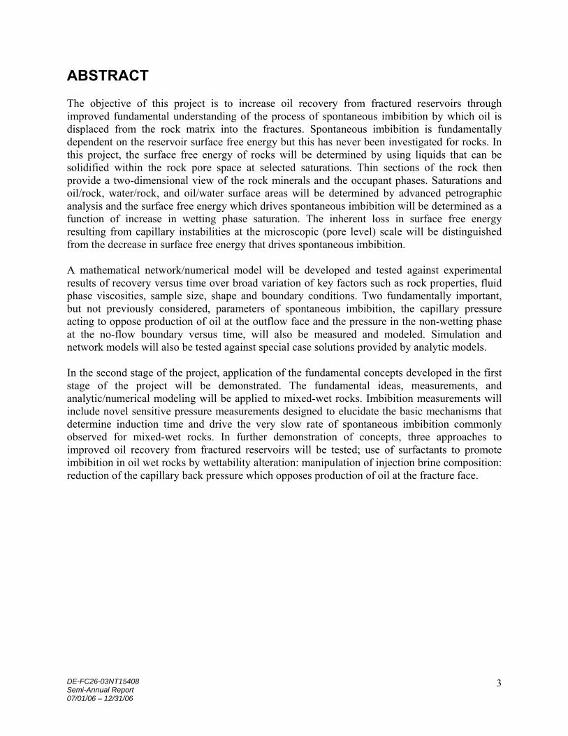
(initially saturated with mineral oil, Swi=25%). (HB3, VSWW,Swi = 25 %) Cores aged with crude oil with an initial water saturation. MXW HD2, MXW,Swi =16.8 % The main core segment was saturated with 83.2% Cottonwood crude oil and 16.8% initial water saturation, and then aged at 75oC for 10 days. The end pressure rose to 2.7 kPa within 1.3 days after the composite core was immersed in brine and remained at about 2.8 kPa until the invading brine reached the dead end (4.5 days after the composite core had been immersed). Results for core HD2 are shown in Fig. 6-7. The end pressure gradually fell over 29 days to 0.3 kPa and then remained close to this value for 16 days.
DE-FC26-03NT15408 Semi-Annual Report 07/01/06 – 12/31/06
13
0.0
0.2
0.4
0.6
0.8
1.0
0 20 40t (days)
Qo/Vφ
xf/Lc
0
2
4
6
8
10
12
14
xf/Lc
PendSwi+Qo/Vφ
Pend
(kPa)
Fig. 6-7 Measurement of Pend (MXW) for core HD2 initially saturated with
crude oil at Swi=16.8% and then aged. HD2, MXW,Swi =16.8 %
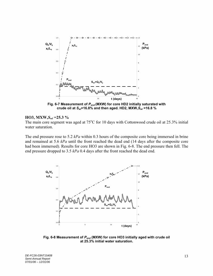
HO3, MXW,Swi =25.3 % The main core segment was aged at 75oC for 10 days with Cottonwood crude oil at 25.3% initial water saturation. The end pressure rose to 5.2 kPa within 0.3 hours of the composite core being immersed in brine and remained at 5.6 kPa until the front reached the dead end (14 days after the composite core had been immersed). Results for core HO3 are shown in Fig. 6-8. The end pressure then fell. The end pressure dropped to 3.5 kPa 0.4 days after the front reached the dead end.
0.0
0.2
0.4
0.6
0.8
1.0
0 5 10 15t (days)
Qo/Vφ
xf/Lc
0
2
4
6
8
10
12
14
xf/Lc
Pend
Swi+Qo/Vφ
Pend
(kPa)
Fig. 6-8 Measurement of Pend (MXW) for core HO3 initially aged with crude oil at 25.3% initial water saturation.

DE-FC26-03NT15408 Semi-Annual Report 07/01/06 – 12/31/06
14
Table 6-1 HIGH
K CORE
D
(cm)
Lc
(cm)
K
(µm2)
φ
(%)
Swi
%
ρo µo
(Pa.s)
Pcf
(kPa)
σ
mN/m
Pcf/σ
(µm-1)
TYPE PROBEOIL
H6O 3.795 6.967 1.067 22.2 0 0.783 0.0038 12.40 48.85 0.254 VSWW Mineral HF4 3.37 3.171 0.964 22.3 0 0.783 0.0038 14.4 48.85 0.295 VSWW Mineral
HC4 3.406 6.555 0.991 22 0 0.8874 0.2041 1.6 29.7 0.054 WWW Crude HE2 3.599 6.332 0.991 22 0 0.8874 0.2041 1.64 29.7 0.055 WWW Crude
HB1 3.343 6.567 0.86 21.5 17.9 0.783 0.0038 4.70 48.85 0.096 VSWW Mineral HB3 3.248 6.555 1.022 22.2 25 0.783 0.0038 3.30 48.85 0.068 VSWW Mineral
HD2 3.151 6.215 1.055 22.7 16.8 0.8874 0.0241 2.66 29.7 0.090 MXW Crude HO3 3.703 6.45 1.026 22 25.3 0.8874 0.0241 5.50 29.7 0.185 MXW Crude
Task 7. Novel imbibition measurements on mixed-wet rock and network models. Countercurrent spontaneous imbibition experiments on oil reservoir rocks are usually carried out using cylindrical cores of rock. Sometimes the cores are sealed on some of the faces, and experiments then give production curves of different duration and slightly different shape. Results can be correlated for rock properties such as porosity and permeability and fluid properties such as viscosity and interfacial tension. An overall or average scale factor correlates for different core sizes and shapes. Although the real imbibition process is actually quite complicated, by making the approximations that there is (a) frontal displacement and (b) constant saturation behind the front, a simple analytical solution is possible. The analysis gives a new shape scale factor. These assumptions also allow the scale factors of Ma et al. and Ruth et al. to be used to predict the shape of the production curves. Countercurrent spontaneous imbibition experiments using matched cores of different shape were carried out to challenge the Ma, Ruth and new scale factors. In particular, cylindrical cores with an axial hole were used with either the inner or outer cylindrical face open to give radial geometry with imbibition into a contracting or expanding volume. The experimental results confirmed that the Ma and Ruth scale factors are good to excellent for most situations but that the new one is marginally better for extreme shape variations. Variability between the cores caused by not having enough exposed surface and not enough rock depth seems to be of greater importance than the differences between the three scale factors.
Introduction to Novel imbibition measurements on mixed-wet rock and network models. Countercurrent spontaneous imbibition occurs when a wetting fluid displaces a less-wetting fluid from the pore space of a porous medium. The wetting fluid imbibes into the pore space and the non-wetting fluid is expelled. In systems with one-dimensional geometry such as a cylinder open at one end and other geometries, the mass balance requirement means that the flows of the two fluids are equal but in opposite directions. Also, experimentally, in some circumstances a saturation front is observed to advance through the system. A positive pressure has to build up at the dead end of the system and it is this pressure that pushes the non-wetting phase back through the invading wetting phase (Li et al., 2003, 2006). Countercurrent imbibition is believed to be a mechanism by which oil can be displaced from the rock in fractured reservoirs (Morrow & Mason, 2001).

DE-FC26-03NT15408 Semi-Annual Report 07/01/06 – 12/31/06
15
Countercurrent imbibition in reservoir rocks is usually studied at the core level using cylindrical cores about 70mm long and with a diameter of about 35 to 50mm. A typical experiment consists of saturating a core with oil and then immersing it in brine. The expelled oil is collected and its volume is measured. Results are recorded as the total amount of oil produced at various time intervals. Attempts have been made to correlate results for very strongly water wet imbibition so that the effect of changing interfacial tension, rock porosity and permeability can be predicted (Mattax & Kyte, 1962). There are two additional factors - the viscosities of the two phases and the shape of the sample. This report addresses the latter problem. Frequently cores used in experiments have all faces of the cylinder open to the invading phase. The experiments give rapid and reproducible results but the flow patterns are complex and, therefore, difficult to model. If the ends of the core cylinder are sealed then the flows become radial. The simplest case, however, reducing imbibition to a one-dimensional, linear situation, is to seal the outer surface plus one end, thus leaving one end open for the imbibition and production to take place. Because the shape of the sample makes a difference to the shape of the production vs time results, it would be convenient to be able to transform experimental results obtained from one core geometry into those from another (Behbahani et al., 2006). A function involving the core sample shape which was found to correlate available data reasonably well is (Ma et al. 1997):
tµµσ
φK
Lt
nww2c
D1
= (7-1)
where cL is a characteristic length, K the rock permeability, φ its porosity, σ is the interfacial tension between the phases and wµ and nwµ are the viscosities of the wetting and non-wetting phases. This expression has been recently applied to cores of different shape (Yildez et al., 2006)
matched viscosities
0.00
0.10
0.20
0.30
0.40
0.50
0.60
0 1 10 100 1000dimensionless time t D
frac
tiona
l oil
reco
very
4 cp14 cp21 cp44 cp59 cp80 cp141 cp
Figure 7-1. Typical experimental data correlated by Eq. (7-1). The data is taken from Fischer &
Morrow, 2006, and is for linear countercurrent spontaneous imbibition into one-end-open cores with similar properties. The two fluids have matched viscosities.

DE-FC26-03NT15408 Semi-Annual Report 07/01/06 – 12/31/06
16
Figure 7-1 shows a correlation (Fischer & Morrow, 2006) for matched viscosities and one end open. In Eq. 7-1, tD is a normalised dimensionless time and it is obtained by multiplying the actual time (t) by a function of rock and fluid properties. Ma’s semi-empirical correlation (1997) for the general characteristic length cL is
∑=
=n
i iA
ix
AVL1 ,
c (7-2)
where V is the bulk volume of the matrix, iA is the area open to imbibition in the ith direction,
iAx , is the distance from iA to the no-flow boundary and n is the number of faces open to imbibition. For linear imbibition cL is simply the length of the core. For a cylindrical core with all faces open it becomes
2max
2
maxc
22 Ld
dLL
+= (7-3)
where maxL is the core length and d is the core diameter. Note that the correlation just brings the data together and on a 10log scale changes in the characteristic length Lc only move the production curves left and right. The characteristic length does not predict the form of the production vs tD function. The function in Eq. 7-1 involves the core permeability K and porosityφ ; σ is the interfacial tension and t is the actual time. Lc is a characteristic length which includes both size and shape and is given by Eq. 7-2. The interesting factor is the nww µµ term because it involves only the viscosities of the wetting and non-wetting phases without any explicit dependence on relative permeabilities. The correlation only involves the time axis; the other axis is usually presented as the fraction of the pore volume filled with wetting phase (i.e. the recovery), although this is sometimes normalised by division by the oil recovered at infinite time. The core shape factor which determines the characteristic length has been investigated in some detail by Ma et al. (1997) and later by Ruth et al. (2003). However, their work was mainly concerned with the general correlation of the imbibition curve's location on a t10log scale rather than the changes in function form brought about by different sample shapes. Recent experiments (Fischer & Morrow, 2005) have demonstrated the small but systematic differences in the form of imbibition production curves particularly between the one-dimensional and all-faces-open configurations that are normally used in experiments. For co-current imbibition Zimmerman et al. (1990) predicted such differences in shape using both numerical simulation and an approximation method. It is the purpose of this report to indicate an a priori shape for the countercurrent imbibition production function and to quantify the small differences in function shape caused by different sample geometry. Frontal Imbibition. General In some cases one-dimensional countercurrent imbibition is primarily a frontal process because, during experiments, a liquid front can be seen to advance along the core (Li et al., 2003). The volume imbibed relative to the core porosity multiplied by the distance that the front has advanced gives an indication of the step change in saturation at the front. The final amount imbibed relative to the total volume of the pore space gives an indication of the final saturation.

DE-FC26-03NT15408 Semi-Annual Report 07/01/06 – 12/31/06
17
From these values one can conclude that about 80% of the imbibition recovery reported by Li et al. occurs as frontal displacement. This does not mean that all countercurrent spontaneous imbibition is a frontal process, just which in some circumstances it is. In simulation of one-dimensional countercurrent imbibition, it has been shown (Li et al., 2003) that the front and its small amount of dispersed imbibition could be represented by a self-similar front. By self-similar we mean that the saturation profile with distance is always the same provided that the distance to the front is properly scaled. The self-similar front is a consequence of the mathematical formulation of countercurrent imbibition. There are three functions, all of saturation; there is the capillary pressure, and two relative permeabilities, one for the wetting phase and the other for the non-wetting phase. The consequence is that, for a thin slice of core, if the relative permeability for one phase is fixed then there is only a single value for the relative permeability for the other phase. Added to this is the fact that, for pure countercurrent spontaneous imbibition, the flow of one phase through the slice is exactly equalled by the reverse flow of the other phase, and both these are over the same area. The concept of a single function representing capillary pressure has been recently challenged by Le Guen & Kovscek (2006) who suggest that non-equilibrium effects should be taken into account. If this behaviour obtains, it would add another variable. As a limiting case, following Cil & Reis (1996), we could imagine that ALL of the saturation change takes place at the saturation front where the saturation makes a step change from Swi (the initial wetting phase saturation) to Swf (the wetting phase saturation at the front). This assumption means that the saturation behind the front is constant at Swf . Behind the front therefore, the relative permeabilities of each of the two phases are also constant. Also, because there is no change in saturation behind the front, the flow of wetting phase ( wq ) at one instant in time is invariant with distance from the open face. Up to the front, the flow of non-wetting phase ( nwq ) is also invariant. It must be stressed that this is an approximation, but it provides a tractable model that may be approximately realistic for some cases of imbibition. Darcy's law gives the two flows:
x
Pµ
AKkq
∂∂
−= w
w
rww (7-4)
x
Pµ
AKkq
∂∂
−= nw
nw
rnwnw (7-5)
where K is the permeability, rwk and rnwk are the relative permeabilities to the respective phases,
wµ and nwµ are the respective viscosities, A is the area and x is a distance. The capillary pressure
cP is the difference between the pressure in the non-wetting phase ( nwP ) and the pressure in the wetting phase ( wP ). wnwc PPP −= (7-6) and flow continuity gives:

DE-FC26-03NT15408 Semi-Annual Report 07/01/06 – 12/31/06
18
nww qq −= (7-7) Combining equations 7-6 to 7-7 gives:
xP
kµkµAkKk
q∂∂
+= c
rwnwrnww
rnwrww (7-8)
Because the saturation has been assumed to be constant behind the front, a large part of this equation will be constant. Let M be a mobility factor and let
rwnwrnww
rnwrw
kµkµkk
M+
= (7-9)
For constant saturation the relative permeabilities have to be constant, consequently the factor M will be constant and so, behind the front
xP
KMAq∂∂
= cw (7-10)
It should be noted that for the assumption that the saturation behind the front is constant to be approximately true, cP has to be able to vary a lot (so as to be able to drive the flows) for negligible changes in wS (i.e. the gradient of the capillary pressure curve with saturation is steep). Because the mobility factor M is constant for the flows behind the wetting front, Eq. 7-10 can be integrated between the open face of the core and the front. For one-dimensional imbibition the area A will be a constant. However, for radial flows into a cylinder with capped ends, the area A will vary with the distance and so the function for the amount of imbibition versus time will be different. It is the effect of the change in areas with distance and its effect on the overall resistance to flow and the changes it makes to the rate of frontal advance that are the main factors in the following analysis. The flow of wetting phase arriving at the front advances the position of the front. A mass balance gives
( )wiwf
wf
dd
SSAφq
tx
−= (7-11)
where xf is the distance of the front from the open face. wiS is the initial saturation and wfS is the saturation behind the front. One Dimensional Countercurrent Imbibition The experimental situation is of a core initially mostly filled with non-wetting phase and sealed on all faces except one end. Starting with Washburn (1921), for co-current imbibition this case

DE-FC26-03NT15408 Semi-Annual Report 07/01/06 – 12/31/06
19
has been investigated many times. It gives the base case with which other core shapes can be compared.
Figure 7-2. Diagram showing linear countercurrent imbibition.
In Eq. 7-10 wq , M and A do not vary with x and so the equation can be integrated between the open face and the front to give: ( ) ( )cocffw 0 PPKMAxq −=− (7-12)
cfP is the capillary pressure difference at the front. Pco is the capillary pressure difference at the open face. At the open face the pressure in the wetting phase is zero but the pressure in the non-wetting phase is not zero It is not zero because non-wetting phase has to be bubbled from the rock into the wetting phase (Li et al., 2006). Substituting for qw using Eq. 7-12 in Eq. 7-11 and integrating between the open face and the distance of the front, xf , gives:
( )
( ) tSSφ
PPKMx
wiwf
cocf2f
2−
−= (7-13)
The time t is zero when the front is at the open face. If f is the fractional amount of non-wetting phase produced at time t, then, for core length Lmax, maxf Lxf = and
( )
( ) tSSφ
PPKML
fwiwf
cocf2max
2 2−
−= (7-14)
For cylindrical tubes the capillary pressure is related to mean pore radius rmean by
mean
c2
rσP = (7-15)
and, again for a bundle of cylindrical tubes, the tube radius is related to the permeability and porosity by (Pirson 1958)
φKr 8
mean = (7-16)

DE-FC26-03NT15408 Semi-Annual Report 07/01/06 – 12/31/06
20
Equation 7-12 contains a difference in capillary pressures ( )cocf PP − . The capillary pressure at the front ( )cfP is mainly produced by the smaller pores and the capillary pressure at the open face ( )coP is mainly produced by the larger pores. The difference between them is thus related to the spread of the pore size distribution. For a spread of pore sizes, ( )cocf PP − can be related to the mean capillary pressure, Pc , by a factor Cspread which is in some way determined by the breadth and shape of the pore size distribution. Just how does not concern us at the moment. Thus
KφσC
rσCPCPP
822
spreadmean
spreadcspreadcocf ===− (7-17)
Eliminating ( )cocf PP − from Eq. 7-14 gives
( ) tSSσMC
φK
Lf
wiwf
spread2max
2 21−
= (7-18)
Comparison of Eq 7-18 with the correlation of Eq. 7-1 shows close similarity. The spread in pore size distributions may well make Cspread constant for related rock types (Berea sandstone, for example). The major difference between the two is the way in which the viscosities of the two phases enter the functions. In Eq. 7-1 it is as the geometric mean and in Eq. 7-18 it is in the mobility factor M as a combination of relative permabilities and viscosities plus the effect of Cspread . Quite why the relative permeabilities would relate in this way with viscosities is still a question to be answered. In Eq. 7-1 the functional form of the fraction filled is unknown whereas in Eq. 7-18 it is simply a squared term. Eq. 7-18 can be rearranged so as to be explicit for t:
( ) 22
maxspread
wiwfLinear, 2
fLσMC
SSKφt f
−= (7-19)
This equation now predicts the time for fractional production f from a core of length maxL for linear imbibition. When experiments are carried out both the time and fractional production are determined. Thus the shape of the experimental production curve can be compared to the theoretical prediction. The time for the front to reach the end of the core, endt , when imbibition ceases will be
( )
σMCSS
KφLt
spread
wiwf2maxend 2
−= (7-20)
This equation is in exact agreement with Ma’s equation which gives the characteristic length for this geometry cL as the length of the core maxL . Note, however, that Eq. 7-19 predicts the actual shape of the production curve.

DE-FC26-03NT15408 Semi-Annual Report 07/01/06 – 12/31/06
21
Radial Countercurrent Imbibition Radial inwards For radial inwards imbibition the core sample is a cylinder with a central cylindrical hole (which may or may not be present), radius closedR , and with both ends and the surface of the inner hole sealed. Imbibition is radial inwards towards the core axis from the outside of the cylinder. At a time t the front has reached a position Rf (measured from the core axis) from its starting position at openR , the core radius, at t = 0 (see Fig. 7-3). Again, by assuming that the core has a constant saturation behind the front, Swf , the total radial flow inwards does not vary with distance behind the front.
Figure 7-3. Diagram of dimensions in radial imbibition. There is a sealed hole in the center of the core so that imbibition takes place from the outside moving in. The total radial flow is constant everywhere behind the front. Compared to linear imbibition, proportionally more of the core is
near the open face. For some general intermediate position, R, between the front and the outside of the core Eq. 7-10 applies
xP
KMAq RR ∂∂
= c,w (7-21)
Unlike the linear case the area, RA , is now a function of R. If the core length is Lcore then the area RA becomes 2πRLcore and ∂x becomes R∂− . Hence
RP
RLπKMq R ∂∂
−= ccore,w 2 (7-22)
As before Rq ,w is invariant (with R) and so Eq. 7-22 can be integrated to give
( )Rq
PPLπKMRR
,w
cocfcore
open
f 2ln
−−= (7-23)
Again Eq. 7-11 gives the distance advanced by the front (-dRf ) in time dt in terms of Rq ,w
( )wiwfcoref
,wf
2dd
SSφLRπq
tR R
−−= (7-24)

DE-FC26-03NT15408 Semi-Annual Report 07/01/06 – 12/31/06
22
except that now the area which was previously constant is now RA , and is a function of Rf . Eliminating Rq ,w between Eq. 7-23 and Eq. 7-24 gives
( )
( ) tSSφ
PPKMRR
RRR
RR
d1dlnwiwf
cocf2openopen
f
open
f
open
f
−−
=⎟⎟⎠
⎞⎜⎜⎝
⎛ (7-25)
Integration of Eq. (7.25) from t = 0, openf RR = to (t, fR ) gives
( )
( ) tSSφ
PPKMRR
RRR
RR
wiwf
cocf2open
2
open
f
open
f
2
open
f 4ln21−
−=⎟
⎟⎠
⎞⎜⎜⎝
⎛−⎟
⎟⎠
⎞⎜⎜⎝
⎛+ (7-26)
Replacing the cP 's with K, φ , and spreadC as before using Eq. 7-17 gives,
( ) tSSσMC
φK
RRR
RR
RR
wiwf
spread2open
2
open
f
open
f
2
open
f 22ln21−
=⎟⎟⎠
⎞⎜⎜⎝
⎛−⎟
⎟⎠
⎞⎜⎜⎝
⎛+ (7-27)
The fraction of the total imbibition when the front is at fR is
2closed
2open
2f
2open
RRRR
f−
−= (7-28)
giving
⎟⎟
⎠
⎞
⎜⎜
⎝
⎛
⎟⎟⎠
⎞⎜⎜⎝
⎛−−=⎟
⎟⎠
⎞⎜⎜⎝
⎛2
open
closed
2
open
f 11RR
fRR (7-29)
Thus
( ) tSSσMC
φK
RRR
ffRR
ffRR
ffwiwf
spread2open
2
open
closed
2
open
closed
2
open
closed 221ln1−
=⎟⎟
⎠
⎞
⎜⎜
⎝
⎛
⎟⎟⎠
⎞⎜⎜⎝
⎛+−⎟
⎟
⎠
⎞
⎜⎜
⎝
⎛
⎟⎟⎠
⎞⎜⎜⎝
⎛+−+⎟
⎟⎠
⎞⎜⎜⎝
⎛−
(7-30) The time taken for the front to reach the centre of the core ( )closedf RR = when imbibition stops, tend , is
( )
σMCSS
KφR
RR
RRtspread
wiwf2closed
open
closed2closed
2openend 2
ln221 −
⎟⎟⎠
⎞⎜⎜⎝
⎛−+= (7-31)
The characteristic length given by Ma’s equation for a solid cylinder of infinite length is 2maxc RL = and Eq. 7-31 agrees exactly with it when 0closed =R . However, when the core has
an inner circular hole, Ma’s method for calculating the characteristic length (Ma et al., 1997) gives

DE-FC26-03NT15408 Semi-Annual Report 07/01/06 – 12/31/06
23
( )
⎟⎟⎠
⎞⎜⎜⎝
⎛+
−=
open
closed2
closedopen2Mac, 1
2 RRRR
L (7-32)
Ruth et al.(2003) improved on this factor by compensating for situations where incremental volumes of the sample do not have the same sizes at different distances from the open face. If the Ruth factor is scaled relative to the Ruth linear function and is factorised one obtains
( )
⎟⎟⎠
⎞⎜⎜⎝
⎛+
−=
open
closed2
closedopen2Ruthc, 21
3 RRRR
L (7-33)
Eq. 7-31 here not only compensates for incremental volumes being at different distances (like Ruth’s) but also compensates for the variation in resistance with distance between the incremental volume and the open face and gives:
⎟⎟⎠
⎞⎜⎜⎝
⎛−+= 2
closedopen
closed2closed
2open
2c ln2
21 R
RRRRL (7-34)
Note that all three scale factors agree when closedR is almost equal to openR and cL equals
closedopen RR − . This is not surprising because the geometry is a thin laminar sheet in which imbibition is linear in theory and there are no effects of the radial geometry. Radial outwards The radial outwards situation is shown in Fig. 4. The equation governing flow is the same as Eq. 7-23 because of the way closedR and openR have been defined.
( )Rq
PPLπKMR
R
,w
cocfcore
closed
f 2ln
−−= (7-35)
The analysis is as before with Rq ,w being invariant with R . Its elimination, followed by integration from 0=t , openf RR = to ( )closed, Rt and replacement of the Pc 's with K, φ , and
spreadC , gives exactly the same equation as Eq. 7-27. Even the equation for the fraction of imbibition, f, is unchanged. It follows that the equation for the time taken for the front to reach the closed boundary, tend , is also unchanged as is the scale factor, 2
cL . Numerically the times and scale factors between radial inwards and radial outwards imbibition will differ because openR and
closedR are different. The basic equations, however, are the same.

DE-FC26-03NT15408 Semi-Annual Report 07/01/06 – 12/31/06
24
Figure 7-4. Diagram showing the variables for a cylindrical core sealed on the outside with
countercurrent imbibition occurring from a cylindrical central hole. Compared to linear imbibition, proportionally more of the core is further from the open face.
Radial scale factors Equations 7-32, 7-33, and 7-34 give the scale factors for the Ma, Ruth and the current analysis (now termed Mason, for short). They are all slightly different and only agree when the hole is virtually the same diameter as the core when imbibition becomes essentially linear. For the radial inwards situation a comparison of the various functions can be made in different ways. Figure 7-5 shows the scale factors plotted against the aspect ratio of the hole in the cylinder and with a cylinder diameter of unity. Considering their different functional form, the Ma and Mason functions are surprisingly close.
0
0.1
0.2
0.3
0.4
0.5
0.6
0 0.2 0.4 0.6 0.8 1 1.2aspect ratio, R closed/R open
scal
e fa
ctor
Ma
Ruth
Mason
Figure 7-5. Comparison of the scale factors calculated using the Ma, Ruth and present (Mason)
functions for radial-inwards imbibition. Note that all three start at the same values when closedR is
almost equal to openR which approximates to the linear situation.
DE-FC26-03NT15408 Semi-Annual Report 07/01/06 – 12/31/06
25
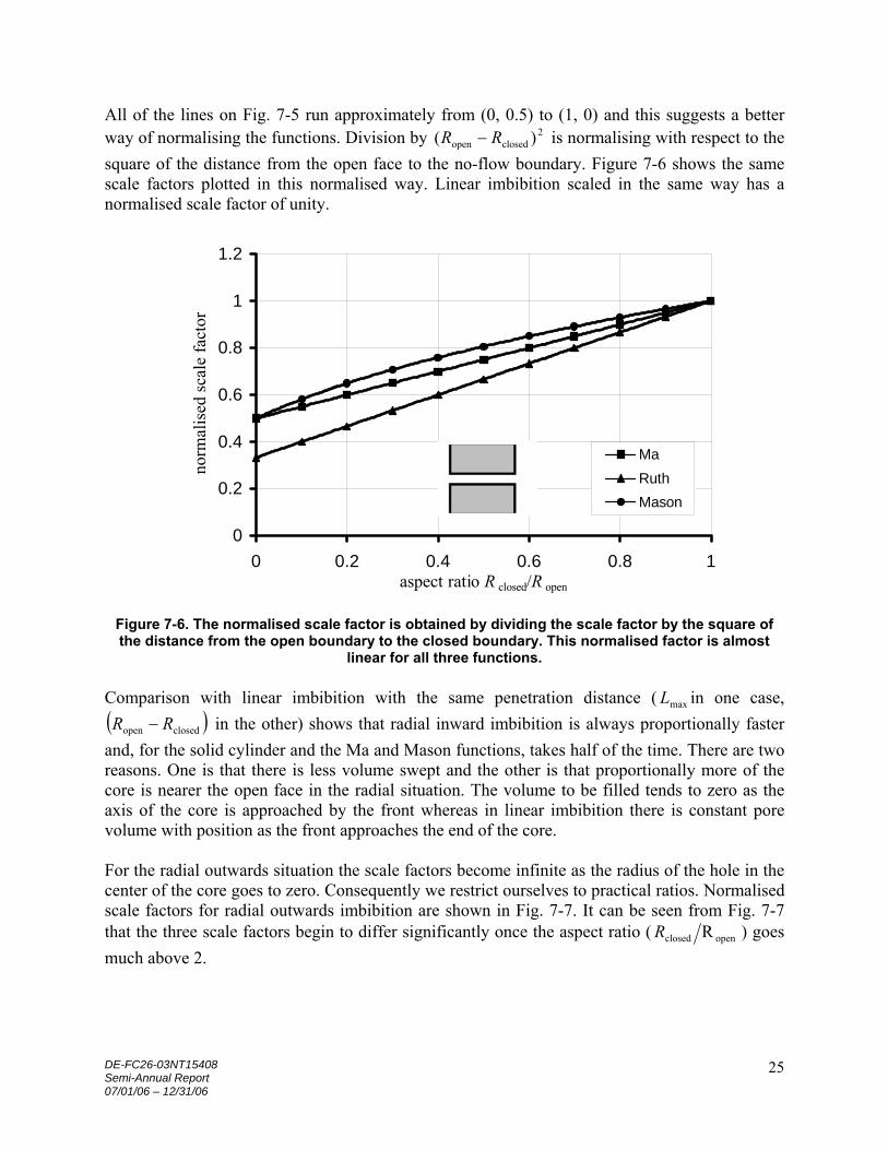
All of the lines on Fig. 7-5 run approximately from (0, 0.5) to (1, 0) and this suggests a better way of normalising the functions. Division by 2
closedopen )( RR − is normalising with respect to the square of the distance from the open face to the no-flow boundary. Figure 7-6 shows the same scale factors plotted in this normalised way. Linear imbibition scaled in the same way has a normalised scale factor of unity.
0
0.2
0.4
0.6
0.8
1
1.2
0 0.2 0.4 0.6 0.8 1aspect ratio R closed/R open
norm
alis
ed sc
ale
fact
or
MaRuthMason
Figure 7-6. The normalised scale factor is obtained by dividing the scale factor by the square of the distance from the open boundary to the closed boundary. This normalised factor is almost
linear for all three functions. Comparison with linear imbibition with the same penetration distance ( maxL in one case, ( )closedopen RR − in the other) shows that radial inward imbibition is always proportionally faster and, for the solid cylinder and the Ma and Mason functions, takes half of the time. There are two reasons. One is that there is less volume swept and the other is that proportionally more of the core is nearer the open face in the radial situation. The volume to be filled tends to zero as the axis of the core is approached by the front whereas in linear imbibition there is constant pore volume with position as the front approaches the end of the core. For the radial outwards situation the scale factors become infinite as the radius of the hole in the center of the core goes to zero. Consequently we restrict ourselves to practical ratios. Normalised scale factors for radial outwards imbibition are shown in Fig. 7-7. It can be seen from Fig. 7-7 that the three scale factors begin to differ significantly once the aspect ratio ( openclosed RR ) goes much above 2.

DE-FC26-03NT15408 Semi-Annual Report 07/01/06 – 12/31/06
26
0
1
2
3
4
5
0 1 2 3 4 5 6 7aspect ratio R closed/R open
norm
alis
ed sc
ale
fact
or
MaRuthMason
Figure 7-7. Radial imbition outwards is where the aspect ratio is greater than unity. Because the normalised scale factors are always above 1 for radial outwards imbibition, imbibition in such a geometry is proportionally much slower than for the linear situation (for which the normalised
scale factor is 1) Fractional production The key assumption has been that frontal imbibition takes place. There is a further consequence of this assumption: imbibition ceases suddenly when the front reaches the closed boundary at the time endt . With cylindrical geometry it was endt that determined the scale factor. Because the front position does not depend on the closed boundary until it actually reaches it, it follows that the shape of the production curve is independent of the actual boundary location. The scale factor ( cL ) is determined by the final front position (i.e. the closed boundary) as well as the core shape. The scale factor is thus the ultimate consequence of the production curve. For radial imbibition and a fractional production of f, the value of fR is given by Eqn(7-28), or explicitly ( )2
closed2open
2open
2f RRfRR −−= (7-36)
Substitution of fR into Eq. 7-27, also 7-37 enables the appropriate time for that fractional production, f, to be found.
( )
⎟⎟⎠
⎞⎜⎜⎝
⎛−+
−= 2
fopen
f2f
2open
spread
wiwfMason, ln2
221 R
RR
RRσMC
SSKφt f (7-37)
Different core geometries produce different shaped production curves. For example, Eq. 7-19 predicts the production versus time function for linear imbibition. The combination of Eq. 7-36 and Eq. 7-37 does the same for radial imbibiton. The two are compared on Fig. 7-8 using the conventional log10 t on the x-axis. Although one is displaced relative to the other, the actual shapes look very similar when plotted in this way.

DE-FC26-03NT15408 Semi-Annual Report 07/01/06 – 12/31/06
27
0
0.5
1
-5 -4 -3 -2 -1 0log10 t
frac
tion
fille
d f Radial
Linear
Figure 7-8. Comparison of linear and radial inwards imbibition. The fraction imbibed is plotted versus t10log . The length of the core in linear imbibition and the radius of the core in radial
imbibition have been set to unity so that the distance the front has to travel is the same in both
geometries. The factor ( )wiwf
spread2SS
MCK−φ
has also been set at 1. No adjustment for the different
characteristic lengths has been made and so the time when imbibition is completed ( endt ) for radial imbibition is half that for linear imbibition.
In order to better emphasise the difference in shape between radial and linear imbibition production curves it is better to use a time axis and to normalise with respect to endt . The comparison is shown in Fig. 7-9.

DE-FC26-03NT15408 Semi-Annual Report 07/01/06 – 12/31/06
28
0
0.2
0.4
0.6
0.8
1
0 0.2 0.4 0.6 0.8 1
frac
tion
fille
d f
RadialLinear
endtt
Figure 7-9. The imbibition curves of Fig. 8 plotted against the square root of normalised time
endtt . This plot clearly shows shows the effect of differences in shape. However, the two production curves are still very similar.
A similar analysis can be followed using the Ma and Ruth scale factors to predict the entire production curve. For radial imbibition the idea can be extended to cover different aspect ratio cores and with imbibition radial inwards or radial outwards and for all three functions (Ma, Ruth, Mason). There are clearly a large number of possible comparisons. However, it is known from past experiments that the shapes of countercurrent imbibition production curves are similar, especially when plotted on the usual log10 t scale. This can be seen from Fig. 7-8. In fact, although they look very different mathematically, the three functions (Ma, Ruth, Mason) give very similar production curves for most practical situations. To show differences one needs to go to unusual core geometries. One such is a core with a central cylindrical hole with a diameter of 0.2 times the core diameter. If sealed on the inside and both ends, this geometry gives radial inwards imbibition with an aspect ratio ( openclosed RR ) of 0.2. If sealed on the outside and both ends, the geometry is radial outwards with an aspect ratio of 5. For the same distance travelled by the front, radial inwards imbibition goes faster than linear imbibition and radial outwards imbibition goes slower. Normalising by the time imbibition is completed, endt , allows comparison of the shapes of the different production curves. Also by plotting the fraction imbibed versus endtt makes the linear imbibition production curve a straight line. Figure 7-10 shows the production curves for a core with a central hole 0.2 times the core diameter for radial inwards, radial outwards and linear imbibition. All three functions agree fairly closely but the Mason function is closest to the two outer limits of the other functions.

DE-FC26-03NT15408 Semi-Annual Report 07/01/06 – 12/31/06
29
Central hole diameter = 0.2D core
0
0.2
0.4
0.6
0.8
1
0 0.2 0.4 0.6 0.8 1 1.2
(t /t end)0.5
frac
tiona
l pro
duct
ion
MaRuthMasonLinear
inwardsoutwards
Figure 7-10. Comparison of the three functions for radial inwards, aspect ratio 0.2 (the three left hand curves) and radial outwards, aspect ratio 5 (the three right hand curves) for a core with an
axial hole diameter of 0.2 times the outer core diameter. Note that all of the curves are similar and, when plotted in this way, are almost linear. For inwards imbibition the Ma and Mason functions are
almost coincident. For outwards imbibition the Ma and Ruth functions are almost coincident. Two important imbibition geometries, linear and radial inwards into a solid core, have frequently been tested by experiment. It has been observed (Fischer et al. 2006) that logarithmic plots of the distance of frontal advance calculated from the fraction imbibed ( fx for linear and ( )fopen RR − for radial) versus time on log-log plots are straight lines. Figure 7-11 shows such plots for the three shape factors. For linear imbibition the plot is a straight line. It is also almost a straight line for the Ma, Ruth and Mason functions. However, extrapolating the straight line to full invasion saturation does not give quite the same time value as the linear case because all three curves have a small highly curved portion near to complete invasion.

DE-FC26-03NT15408 Semi-Annual Report 07/01/06 – 12/31/06
30
-1.8
-1.6
-1.4
-1.2
-1
-0.8
-0.6
-0.4
-0.2
0
-3 -2.5 -2 -1.5 -1 -0.5 0
log10(t )
log 1
0(no
rmal
ized
fron
t pen
etra
tion
dist
ance
)
Ma Radial
Ruth Radial
Mason Radial
Linear
Figure 7-11 Log-log plots of the front position calculated from the fraction imbibed, f, for radial
and linear imbibition. Note that the plots for radial imbibition are very close to being straight lines but, because of the curved parts at higher saturation, the time at which the extrapolated straight
lines reach the maximum front penetration distance is longer than for the curves given by the shape factors.
A fairly simple geometry for which experiments can be readily performed is a cylindrical core with a central axial hole and with both flat ends sealed. Such a geometry exhibits simultaneous outward imbibition from the central hole and inwards imbibition from the outer surface. It is difficult to predict the scale factors using the Ma and Ruth methods because the position of the no-flow boundary is not obvious. However, the concept of frontal imbibition indicates that at the end of imbibition the no-flow boundary will be located at a radius which makes the two scale factors (one inward, one outward) the same. The end point and associated no-flow boundary are connected by the same scale factor. If nfR is the radius at this no-flow boundary then, at the end of imbibition, nfR is the same for the radial inwards front and the radial outwards front. If outerR and innerR are the two core boundary radii then, for the Ma function, Eq. 7-32 gives
( ) ( )
⎟⎟⎠
⎞⎜⎜⎝
⎛+
−=⎟⎟
⎠
⎞⎜⎜⎝
⎛+
−=
inner
nf2
nfinner
outer
nf2
nfouter2Mac, 1
21
2 RRRR
RRRR
L (7-38)
A similar equation can be written for the Ruth function, Eq. 7-33 and for the Mason function, Eq. 7-34. The Ma and Ruth functions both give cubics for nfR but the Mason function gives an analytic expression for the final position of the no-flow boundary
( )
⎟⎟⎠
⎞⎜⎜⎝
⎛−
=
2inner
2outer
2inner
2outer2
nf
lnRR
RRR (7-39)

DE-FC26-03NT15408 Semi-Annual Report 07/01/06 – 12/31/06
31
If imbibition is not complete then the fronts are at two different positions. No analytic solution for the positions of the two fronts is possible and numerical solutions are required.
Experimental Countercurrent spontaneous imbibition experiments were carried out on a series of cylindrical matched Berea Cx sandstone cores which had been cut to have different diameter holes in the center and which had different faces sealed with epoxy resin so that imbibition would be linear, radial inwards or radial outwards. The aims were to find out if any differences in the shapes of the production versus time curves could be detected and how the scale factor, 2
cL , varied with the dimensions. This rock is characterised by a very narrow air permeability range close to 70 md. Because of the unusual core shapes the relevant permeability of every core was not measured.
TABLE 7-1. CORE PROPERTIES
Linear –One End Open Core No. Length
(cm) Outer dia (cm)
Inner dia (cm)
Aspect ratio
Initial volume oil (mL)
Porosity Permeability (mD)
C4-9 6.50 5.13 0 0 21.99 0.163 C4-8 6.62 5.13 0 0 23.59 0.172 C4-12 6.47 5.13 1.03 0.204 20.20 0.157 C-1 5.90 5.07 2.23 0.440 15.37 0.160 C1-25 5.97 5.07 3.01 0.593 12.48 0.159 71.50 C1-24 5.72 5.07 4.16 0.821 5.55 0.148 59.71 C1-25 5.93 5.07 4.15 0.818 5.47 0.138
Linear –Both Ends Open Core No. Length
(cm) Outer dia (cm)
Inner dia (cm)
Aspect ratio
Initial volume oil (mL)
Porosity Permeability (mD)
C4-5 6.50 5.13 0 0 22.45 0.167 C1-25 6.32 3.48 0 0 9.50 0.158 C4-11A 6.58 5.13 1.03 0.201 21.23 0.163 C-5 5.88 5.06 2.22 0.439 15.67 0.164 C4-4 6.55 5.13 2.19 0.427 16.44 0.148 C-7 5.92 5.07 3.02 0.595 12.69 0.164 C4-6 6.10 5.12 3.01 0.588 12.90 0.157 C1-26 5.99 5.06 4.15 0.819 6.27 0.157 67.83 C-9 6.13 5.07 4.15 0.818 6.03 0.147
Radial Inwards Core No. Length
(cm) Outer dia (cm)
Inner dia (cm)
Aspect ratio
Initial volume oil (mL)
Porosity Permeability (mD)
C4-10 6.57 5.13 0 0 23.10 0.170 C4-11 6.50 5.13 1.02 0.199 21.86 0.169 C-8 5.88 5.06 2.23 0.440 16.13 0.169 C4-14 6.15 5.13 3.00 0.585 13.61 0.163 C1-28 5.88 5.07 4.14 0.816 6.52 0.164 70.80

DE-FC26-03NT15408 Semi-Annual Report 07/01/06 – 12/31/06
32
Radial Outwards Core No. Length
(cm) Outer dia (cm)
Inner dia (cm)
Aspect ratio
Initial volume oil (mL)
Porosity Permeability (mD)
C4-13A 6.53 5.14 1.02 5.04 21.38 0.165 C4-1 6.41 5.13 2.25 2.28 17.53 0.163 C1-21 6.20 5.07 3.02 1.68 13.16 0.162 72.19 C1-22 5.71 5.07 4.16 1.22 6.36 0.167 69.70
Radial Inwards and Outwards Core No. Length
(cm) Outer dia (cm)
Inner dia (cm)
Aspect ratio
Initial volume oil (mL)
Porosity Permeability (mD)
C4-10 6.57 5.13 0 0 23.10 0.170 C4-13 6.56 5.13 1.01 0.2 22.84 0.175 C-2 6.09 5.06 2.22 0.44 16.75 0.169 C-11 5.73 5.07 3.01 0.59 12.89 0.173 C1-19 6.22 5.07 4.13 0.81 7.45 0.176 69.88 After the cores were cut, they were dried, evacuated and filled with oil. Their porosity was calculated from the weight difference between the empty and oil-filled states. Oil recovery versus time was measured in standard glass imbibition cells at ambient temperature. The oil was Soltrol 220 and had a viscosity of 3.996 cp. The invading phase was brine with a viscosity of 1.147 cp. The interfacial tension was 45.2 dynes/cm. Linear imbibition was conducted with cores filled with oil and sealed on all faces except one end. The data is shown in Figure 7-12. Different maximum volumes of brine are imbibed because some cores had large holes in them. Also the cores did not have identical length.
0
2
4
6
8
10
12
0 200 400 600 800 1000 1200 1400 1600 1800
time/ (mins)
volu
me/
(mL)
C4-9 AR=0
C4-8 AR=0
C4-12 AR=0.20
C-1 AR=0.44
C1-25 AR=0.59
C1-24 AR=0.82
C1-25 AR=0.82
Figure 7-12. Imbibition volume vs time results for linear (one-end-open) countercurrent imbibition into cylindrical cores with axial holes. The cores have different pore volumes because they have
holes in the middle and are of slightly different lengths.

DE-FC26-03NT15408 Semi-Annual Report 07/01/06 – 12/31/06
33
Similar experiments were performed on cores sealed on the inside and outside but with both ends open. Imbibition thus took place from both ends simultaneously. The results are shown in Fig. 7-13,
0
2
4
6
8
10
12
0 50 100 150 200 250 300 350 400
time/ (min)
volu
me/
(mL) C4-5 AR=0
C1-25 AR=0C4-11A AR=0.20C-5 AR=0.44C4-4 AR=0.43C-7 AR=0.60C4-6 AR=0.59C1-26 AR=0.82C-9 AR=0.82
Figure 7-13. Imbibition volume versus time for linear imbibition into cores with both ends open.
Note that imbibition is much faster than with only one end open (compare with Fig. 7-12). There were three radial boundary conditions. If the only face left open is the outer one then imbibition is radial inwards. If the inner face is the only face open then imbibition is radial outwards. If both faces are open there is combined inwards and outwards radial imbibition. Results for radial inwards are shown in Figure 7-14. If there is frontal imbibition and the core properties were identical then the initial production curves for radial inwards imbibition should all fall on the same curve. This is because all of the cores have almost the same open face dimension and the position of the closed boundary cannot affect the front until the front reaches it. It can be seen that the production curves do all start together, although when the aspect ratio is 0.82 the production curve soon starts to fall off. Results for radial outwards imbibition are shown in Figure 7-15. Because the cores all had the same outer diameter but had different diameter holes cut along the axis, the radius of the open face was now different from core to core. Consequently the production curves should have significantly different shapes. It can be seen that this is actually the case and imbibition from a small radius hole outwards is almost linear. The reason is that most of the pressure drop occurs close to the inner open boundary and so the front position makes little difference to the production rate.

DE-FC26-03NT15408 Semi-Annual Report 07/01/06 – 12/31/06
34
0
2
4
6
8
10
12
0 20 40 60 80time/ (min)
volu
me/
(mL)
C4-10 AR=0
C4-11 AR=0.2
C-8 AR=0.44
C4-14 AR=0.58
C1-28 AR=0.82
Figure 7-14. Production volume vs time for imbibition into cores with all faces except the outer
surface sealed.
0
2
4
6
8
10
12
0 20 40 60 80 100 120 140
time/ (min)
volu
me/
(mL)
C1-22 AR=1.22C1-21 AR=1.69C4-1 AR=2.27C4-13A AR=5.0
Figure 7-15. Production volume vs time results for imbibition into cores with all faces except the
surface of the axial hole in the core sealed. Note that for the highest aspect ratio imbibition is almost linear with time.
Results for combined radial inwards and outwards imbibition are shown in Fig. 7-16. Note that, as would be expected, the time taken for imbibition to be completed is much shorter.

DE-FC26-03NT15408 Semi-Annual Report 07/01/06 – 12/31/06
35
0
2
4
6
8
10
12
0 10 20 30 40 50 60 70 80time/ (min)
volu
me/
(mL)
C4-10 AR=0
C4-13 AR=0.2
C-2 AR=0.44
C-11 AR=0.59
C1-19 AR=0.82
Figure 7-16. Production volume vs time results for cores with both ends closed. Imbibition takes
place for all except C4-10 from both the inside hole and the outside surface. Consequently imbibition is much faster.
Interpretation of experimental results. The experimental results need to be compared with the predictions of the theory. This is not as simple as it seems. The first question is whether or not the theory can match the shape of the production curve. The second question is whether the physical properties of the rock-oil-brine system predicted by the different scale factors are consistent between the linear, radial inwards and radial outwards experiments. Fractional production can be determined for every experiment. This fraction can be inserted into the relevant functions relating time to fractional production (Eq. 7-36 and Eq. 7-37) and a time (multiplied by a constant factor) determined. Let the time calculated from f be ft . For linear imbibition Eq. (7-187) rearranges into
( ) 22
maxspread
wiwfMason Linear,, 2
fLσMC
SSKφt f
−= (7-40)
and for the Ma-Ruth function
22max
nwwMaMaLinear,, fL
σµµ
KφCt f = (7-41)
where MaC is a constant. Let
( )
σMCSS
KφG
spread
wiwfMason 2
−= (7-42)
and
DE-FC26-03NT15408 Semi-Annual Report 07/01/06 – 12/31/06
36
σ
µµKφCG nww
MaMa = (7-43)
As functions of f, Eq. 7-40 and Eq. 7-41 differ only by the arbitrary constants MasonG and MaG . Both Equations 7-40 and 7-41 predict that the fraction imbibed during linear imbibition varies as the square root of time. This is not surprising because the driving pressures are constant but the resistances to flow vary as the distance that the front has advanced. In Equations 7-40 and 7-41 the core length is a parameter and this is best incorporated with f. Thus a plot of 22
max fL versus the actual time for the fractional production f should be a straight line. Actually, because the production varies as the square root of time, it is better to take the square root of both axis variables because this spreads out the experimental points better. We thus have
Mason
Mason Linear,,max G
tfL f
= (7-44)
and
Ma
Ma Linear,,max G
tfL f
= (7-45)
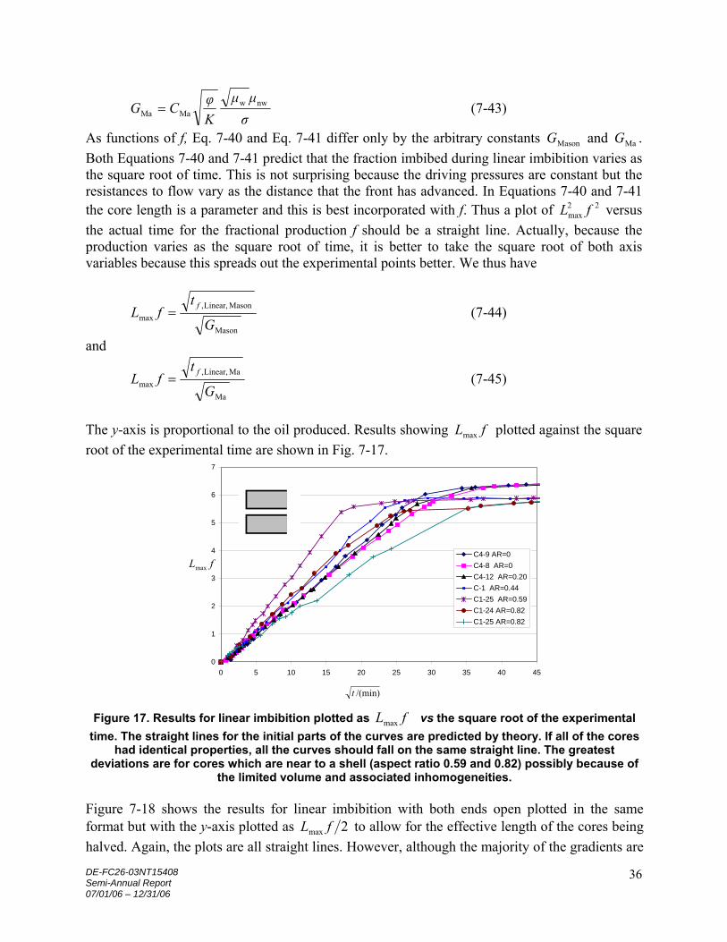
The y-axis is proportional to the oil produced. Results showing fLmax plotted against the square root of the experimental time are shown in Fig. 7-17.
0
1
2
3
4
5
6
7
0 5 10 15 20 25 30 35 40 45
C4-9 AR=0C4-8 AR=0C4-12 AR=0.20C-1 AR=0.44C1-25 AR=0.59C1-24 AR=0.82C1-25 AR=0.82
/(min)t
fLmax
Figure 17. Results for linear imbibition plotted as fLmax vs the square root of the experimental
time. The straight lines for the initial parts of the curves are predicted by theory. If all of the cores had identical properties, all the curves should fall on the same straight line. The greatest
deviations are for cores which are near to a shell (aspect ratio 0.59 and 0.82) possibly because of the limited volume and associated inhomogeneities.
Figure 7-18 shows the results for linear imbibition with both ends open plotted in the same format but with the y-axis plotted as 2max fL to allow for the effective length of the cores being halved. Again, the plots are all straight lines. However, although the majority of the gradients are

DE-FC26-03NT15408 Semi-Annual Report 07/01/06 – 12/31/06
37
the same, the one for C4-11A is significantly different. There are two open faces for these cores and thus the possibility that imbibition will predominantly take place at one face and production from the other. The equations for flow indicate that ahead of the front there is a constant pressure in the non-wetting phase. This dead-end pressure drives the non-wetting phase back through the wetting phase and overcomes the capillary back pressure at the open face. When there are two open faces it may be that the capillary back pressures at the open faces are not equal or, because of inhomogeneity in the core, the permeability may not be evenly distributed. In both of these cases the rate of frontal advance will not be symmetric between the core ends. The production pattern should still vary linearly with the square root of time, but the gradient will be different.
0
0.5
1
1.5
2
2.5
3
3.5
4
0 5 10 15 20 25
C4-5 AR=0
C1-25 AR=0
C4-11A AR=0.20
C-5 AR=0.44
C4-4 AR=0.43
C-7 AR=0.60
C4-6 AR= 0.59
C1-26 AR=0.82
C-9 AR=0.82
/(min)t
2max fL
Figure 7-18. Results for linear imbibition with both ends open plotted as 2max fL versus the
square root of the measured time. The scale factor allowing for the different effective length has been incorporated and so ideally the gradients of these functions should be the same as in Fig. 7-
17. All of the scale factors predict that these functions should be straight lines.
The same method can be followed for radial imbibition. Now, however, the Ma, Ruth and Mason functions give different predictions. Eq. 7-36, gives fR as a function of f
( )2closed
2open
2open
2f RRfRR −−= (7-45)
Then
( )
⎟⎟⎠
⎞⎜⎜⎝
⎛+
−=
open
2opennww
MaMa, 12 R
RRRσ
µµKφCt ff
f (7-46)
( )
⎟⎟⎠
⎞⎜⎜⎝
⎛+
−=
open
2opennww
MaRuth, 213 R
RRRσ
µµKφCt ff
f (7-47)
and
( )
⎟⎟⎠
⎞⎜⎜⎝
⎛−+
−= 2
open
f22open
spread
wiwfMason, ln2
21
2 fff RRRRR
σMCSS
Kφt (7-48)

DE-FC26-03NT15408 Semi-Annual Report 07/01/06 – 12/31/06
38
If we define
( )
⎟⎟⎠
⎞⎜⎜⎝
⎛+
−=
open
openMa 2 R
RRRF ff
f 12
2, (7-49)
( )
⎟⎟⎠
⎞⎜⎜⎝
⎛+
−=
open
openRuth 3 R
RRRF ff
f 212
2, (7-50)
⎟⎟⎠
⎞⎜⎜⎝
⎛−+= 2
open
f22openMason fff R
RR
RRF ln2212
, (7-51)
then the squares of these F factors are proportional to the appropriate times ( Ma,ft , Ruth,ft , Mason,ft ). Thus plotting the squares of the F factors against the actual experimental times for the same fractional production, f, should give straight lines through the origin. Again, to spread out the data points approximately with the volume of oil produced, it is better to plot the square roots of both axis variables. The results should still be straight lines. Figure 7-19 shows the results for radial inwards imbibition. In order to generate these plots, the experimental fractional productions, f, were used in Eq. 7-45 to determine a series of fR ’s. Then these value of fR were used to calculate the three values of fF using Eq. 7-49 to Eq. 7-51. All of the plots are generally linear. At short and even medium times there is not much to choose between the three functions. However, at longer times the differences are significant, especially for the low aspect ratio cores. Because the Mason factor is linear for the longest times for the low aspect ratio core, it is marginally the best. Figure 7-20 shows the results for radial outwards imbibition. Again for the high aspect ratio core the Mason factor produces the closest approximation to linearity, but otherwise there is not much difference between them, and virtually no difference at short times. Results for the two ends closed cores which had simultaneous radial inwards and outwards imbibition were more difficult to analyse. Consequently they have only been interpreted using the Mason function. Essentially two versions of Eq. 7-37 were used, one for the outer front position and the other for the inner front position but with the times to reach these positions equal. Also, the fraction filled depends on the positions of both fronts. Consequently, for a fixed fraction filled, an iterative routine calculated the position of the two fronts and also the resulting time. Knowing the position of the front associated with an open face enabled Mason,fF to be calculated using Eq. 7-51. Figure 7-21 shows the results. They are, again, except for the high aspect ratio core, close to being straight lines with the same gradient.

DE-FC26-03NT15408 Semi-Annual Report 07/01/06 – 12/31/06
39
C4-10, AR=0
0
0.2
0.4
0.6
0.8
1
1.2
1.4
1.6
1.8
2
0 2 4 6 8 10
MaRuthMason
/(min)t
Mason,
Ruth,
Ma,
f
f
f
FF
F
C4-11, AR=0.2
0
0.2
0.4
0.6
0.8
1
1.2
1.4
1.6
1.8
0 2 4 6 8 10
Ma
Ruth
Mason
/(min)t
Mason,
Ruth,
Ma,
f
f
f
F
F
F
C-8, AR=0.44
0
0.2
0.4
0.6
0.8
1
1.2
1.4
0 2 4 6 8 10
MaRuthMason
/(min)t
Mason,
Ruth,
Ma,
f
f
f
F
F
F
C4-14, AR=0.580
0.2
0.4
0.6
0.8
1
0 1 2 3 4 5 6
Ma
Ruth
Mason
Mason,
Ruth,
Ma,
f
f
f
F
F
F
/(min)t
C1-28, AR=0.820
0.1
0.2
0.3
0.4
0.5
0 1 2 3 4 5
Ma
Ruth
Mason
Mason,
Ruth,
Ma,
f
f
f
F
F
F
/(min)t Figure 7-19. Comparison of the three functions for radial inwards imbibition for cores with five
different aspect ratios. The gradients are all similar and close to the gradients for linear imbibition in Figs 7-17 and 7-18. The Mason function is closest to linearity. Only the gradient for imbibition
with an aspect ratio of 0.82 differs significantly, it being too low by a factor of about 2. Because it is a thin shell (it was about 5mm thick) the leading part of the imbibition front may reach the
closed boundary before the front is fully developed.

DE-FC26-03NT15408 Semi-Annual Report 07/01/06 – 12/31/06
40
C1-22, AR=1.22
0
0.1
0.2
0.3
0.4
0.5
0 1 2 3 4
Ma
Ruth
Mason
Mason,
Ruth,
Ma,
f
f
f
F
FF
/(min)t
C1-21, AR=1.69
0
0.2
0.4
0.6
0.8
1
1.2
1.4
0 2 4 6 8
Ma
Ruth
Mason
Mason,
Ruth,
Ma,
f
f
f
F
F
F
/(min)t
C4-1, AR=2.27
0
0.25
0.5
0.75
1
1.25
1.5
1.75
2
0 2 4 6 8 10
Ma
Ruth
Mason
Mason,
Ruth,
Ma,
f
f
f
F
F
F
/(min)t
C4-13A, AR=5.0
0
0.5
1
1.5
2
2.5
3
3.5
4
0 5 10 15
Ma
Ruth
Mason
Mason,
Ruth,
Ma,
f
f
f
F
F
F
/(min)t Figure 7-20. Radial outwards imbibition for cores with four different aspect ratios. There are only
significant differences between the three functions for the high aspect ratio core (AR 5.0).
0
0.2
0.4
0.6
0.8
1
1.2
1.4
1.6
1.8
0 2 4 6 8 10
C4-10 AR=0C4-13 AR=0.2C-2 AR=0.44C-11 AR=0.59C1-19 AR=0.82
(min)t
Mason,fF
Figure 7-21. Results for both ends closed. The analysis is more difficult for this case because there are two fronts moving radially in opposite directions at different different places and at different rates. Except for the most extreme aspect ratio (0.82), the results give close-to straight lines of
almost the same gradient. Some times are very short, making the experiments relatively inaccurate, especially for high aspect ratios. Core C4-10 has no hole in the middle (the results are also in Fig. 7-19). The square of the reciprocal of the gradients is about 20 for all of these cores,
similar to Figs 7-17 to 7-20.

DE-FC26-03NT15408 Semi-Annual Report 07/01/06 – 12/31/06
41
The reciprocal of the squares of the gradients of all of the functions for all of the results were calculated. These are typically gradients for about 75% of the recovery. For Figs 19 to 21 one might arguably subtract about half a minute (or a quarter, when squared) from the start times. These reciprocal gradients are the G values (Eqs. 7-42 and 7-43) and ideally all of these gradients would be the same. A general gradient has been taken for both the linear situations. However, the spread of the experimental values for linear imbibition does give an indication of the variability between the cores. The squares of the gradients are shown on Fig. 7-22 with the ‘both ends closed’ results omitted because they were only calculated for the Mason function and the aspect ratio varies with the predicted position of the no-flow boundary. The aspect ratio of 1 covers all of the linear imbibition results (one end or both ends open).
0
5
10
15
20
25
30
35
40
45
50
0 1 2 3 4 5 6
aspect ratio
prop
ertie
s fac
tor,
G Ma
Ruth
Mason
Figure 7-22. Comparison between the squares of the reciprocals of the gradients of Figs 7-17 to 7-20. These gradients are the G factors defined by Eqs. 7-42 and 7-43. Because they are properties of just the rock and fluids, they should, if the shape factor is correct, ideally all have the same value. Because it gives the most consistent G factor, the Mason scale factor probably the best of the three. The value for an aspect ratio of
0.82 which is too high by a factor of two. This is probably because it is only a thin shell about 5mm thick and has relatively little area open to imbibition which makes it subject to significant error.
In order to test how well the Mason function fits the shape of the production curves, the amount of oil produced as a function of time was calculated for all of the radial outwards experiments using a fixed value of 15 for the factor. The results are shown on Fig. 7-23. The early time data shows a reasonable fit except for AR=5. The function over-predicts production at short times. The linear and radial inwards production curves do not vary much in shape and are not shown.

DE-FC26-03NT15408 Semi-Annual Report 07/01/06 – 12/31/06
42
0
2
4
6
8
10
0 20 40 60 80 100 120
time/(min)
volu
me/
(mL)
C1-22 AR=1.22
C1-22 calc.
C1-21 AR=1.69
C1-21calc.
C4-1 AR=2.27
C4-1 calc.
C4-13A AR=5.0
C4-13A calc.
Figure 7-23. Comparison between experimental measurements and calculated values for radial
outwards imbibition. Except for an aspect ratio of 5 the fits are quite good for the first 70% of the volume imbibed.
Discussion The properties factor G can be obtained from the squares of the reciprocal gradients of the Mason fits in Figures 17-21. Ideally, because the same rock and fluid has been used throughout, all of these gradients should be the same. Set against this is the vast range of times for imbibition to be virtually complete; 2 minutes for the fastest and 1000 minutes for the slowest. Figure 24 shows the G values plotted against the core aspect ratio. Theory predicts that imbibition into one-end-open and two-ends-open cores should be independent of the aspect ratio. However, even for these geometries it can be seen that there is considerable scatter. The aspect ratio 0.82 gives the biggest spread. The values for radial outwards imbibition are marginally lower than the values for radial inwards imbibition. However, overall, the intrinsic variability between experiments seems to be greater than the errors incurred by differences in the shape factors. The cores have a range of volumes and this may go some way to explaining the variability. Also the capillary back pressure required to force oil from the cores is produced by the biggest connected pores at the open face and, statistically, this will probably depend on the surface area of the cores. If we take an overall average value for G of about 20 then Eq. 7-42 gives
( )
σMCSS
KφG
spread
wiwfMason 2
−= (7-42)
The dimensions of G are -2TL . Converting into internally consistent units and taking typical values for porosity and permeability gives

DE-FC26-03NT15408 Semi-Annual Report 07/01/06 – 12/31/06
43
spreadrnww
nw
rww
100011 Ckµ
µkµM
≈+= (7-52)
The viscosity ratio was about 3.5. Using the data of Li et al (2006) the value of spreadC can be estimated to be between 0.5 and 1. Consequently rwk cannot be less than 0.002 and rnwk cannot be less than 0.007. If rwk and rnwk are about equal then they will be about 0.009. Of course if
spreadC is less or the capillary pressure at the front is not determined by the Leverett radius (and interfacial tension) then the relative permeabilities will be higher.
0
5
10
15
20
25
30
35
40
45
50
0.00 1.00 2.00 3.00 4.00 5.00 6.00aspect ratio
prop
ertie
s fac
tor,
G
One end openTwo ends openOuter face openInner face openTwo ends closed
Figure 7-24. The properties factor G plotted against aspect ratio. Ideally, because the rock and
fluids are the same, the value of G should be constant. It seems that the widest spread of values is for the cores with an aspect ratio of 0.8. These are only a thin shell and this may account for the
spread of results. The G factors are plotted against the surface area open for imbibition in Fig 7-25. It can be seen that the most consistent values are obtained for radial imbibition (especially inwards), provided that results for aspect ratio 0.82 are ignored. This implies that there is a critical thickness certainly greater than 0.5mm and maybe less than 15mm, above which consistent results are obtained and below which imbibition seems to occur more slowly. Also, there seems to be a critical area for the open face of about 50 square cm. Exceeding this seems to give more-consistent results. It may be that at least this area is required to give access to the largest pores and thus the lowest and most-consistent capillary back pressure. With too little area the capillary back pressure will likely to be too high with the result that imbibition will be slower, and thus G higher.

DE-FC26-03NT15408 Semi-Annual Report 07/01/06 – 12/31/06
44
0
10
20
30
40
50
60
70
0 50 100 150 200area/(cm2)
prop
ertie
s fac
tor,
GOne end openTwo ends openOuter face openInner face openTwo ends closed
Figure 7-25. The properties factor G plotted against the area open to imbibition. The most consistent values occur with a surface area between 50 and 100 cm2 and, from Fig. 25, core thickness greater than 15 mm. The
two highest values for G come from cores with an aspect ratio of 0.82 which are only 5mm thick.
References Behbahani, H.S., Donato, G.D. & Blunt, M.J., 2006, Simulation of counter-current imbibition in
water-wet fractured reservoirs, J. Petroleum Science & Engineering, 50, 21-39. Cil, M. & Reis, J.C., 1996, A multi-dimensional, analytical model for counter-current water
imbibition into gas-saturated matrix blocks, J. Petroleum Science & Engineering, 16, 61-69. Fischer, H. & Morrow, N.R., 2005, Spontaneous imbibition with matched viscosities, SPE
Preprint 96812, SPE Annual Technical Conference, Dallas, Texas, 2005. Fischer, H. & Morrow, N.R., 2006, Scaling of oil recovery by spontaneous imbibition for wide
variation in aqueaous phase viscosity with glycerol as the viscosifying agent, Journal of Petroleum Science and Engineeering, 52, 35-53.
Le Guen, S.S. & Kovscek, A.R., 2006, Nonequilibrium effects during spontaneous imbibition, Transport in Porous Media, 63, 127-146.
Li, Y., Morrow, N.R. & Ruth, D., 2003, Similarity solution for linear counter-current spontaneous imbibition, Journal of Petroleum Science and Engineering, 39, 309-326.
Li, Y, Ruth, D., Mason, G., & Morrow, N.R., 2006, Pressures acting in counter-current spontaneous imbibition, Journal of Petroleum Science and Engineeering, 52, 87-99.
Mattax, C.C. & Kyte, J.R., 1962, Imbibition oil recovery from fractured, water drive reservoirs, Society of Petroleum Engineers Journal, June 1962, 117-.
Ma, S., Morrow, N.R. & Zhang, X., 1997, Generalized scaling of spontaneous imbibition data for strongly water-wet systems, Journal of Petroleum Science and Engineeering, 18, 165-178.
Morrow, N.R. & Mason, G., 2001, Recovery of oil by spontaneous imbibition, Current Opinion in Colloid & Interface Science, 6, 321-337.
Pirson, S., 1958, Oil Reservoir Engineering, McGraw-Hill New York.

DE-FC26-03NT15408 Semi-Annual Report 07/01/06 – 12/31/06
45
Ruth, D., Mason, G. & Morrow, N.R., 2003, A numerical study of the influence of sample shape on spontaneous imbibition, Proceedings of the Society of Core Analysts Symposium, Pau, SCA2003-16, 1-12.
Washburn, E.W., 1921, The dynamics of capillary flow, Physical Review, 17, 273-283. Yildez, H.O., Gokmen, M, & Cesur, Y., 2006, Effect of shape factor, characteristic length, and
boundary conditions on spontaneous imbibition, J. Petroleum Science & Engineering, 53, 158-170.
Zimmerman, R.W., Bodvarsson, G.S. & Kwicklis, E.M., 1990, Absorption of water into porous blocks of various shapes and sizes, Water Resources Research, 26, 2797-2806.
Task 8. Application of network/numerical model to mixed wet rocks. Experiments that illustrate and quantify the basics of co- and countercurrent spontaneous imbibition have been conducted in a series of simple model pore systems. The fundamental pore geometry is a rod in an angled round-bottomed slot with the rod touching a capping glass plate. The capillaries thus formed by the surfaces of the slot, rod and plate do not have circular cross-sections but more complicated geometric structures with angular corners. The tubes formed at each side of the rod connect at both ends. A viscous, refined oil was applied from one end. For co-current experiments, the opposite end was left open to the atmosphere and oil imbibed into both tubes. For countercurrent experiments the opposite end was sealed and connected to a sensitive pressure transducer. Oil imbibed into the smaller capillary and expelled air as a series of bubbles from the end of the larger capillary. Bubble snap-off was observed to be rate-dependent and occurred at a lower curvature than that of the cylindrical meniscus that just fits inside the tube. Only the corners of the larger capillary filled with oil during countercurrent imbibition. Meniscus curvatures were calculated using the Mayer and Stowe-Princen method and were compared with actual values by measuring the capillary rise in the tubes; agreement was close. A simple model for co-current and countercurrent imbibition has also been developed and the predictions compared with the experimental results. The model results were in agreement with the experiments. The experiments demonstrate that the capillary back pressure generated by the interfaces and bubbles in countercurrent imbibition can slow the process significantly.
Introduction of Application of network/numerical model to mixed wet rocks. A key process in the production of oil from fractured reservoirs is spontaneous imbibition. Such spontaneous imbibition may be either co-current or countercurrent, the second being more common. The main difference between the two mechanisms for imbibition is the direction of flow. In a co-current displacement the wetting and the non-wetting fluids move in the same direction with the non-wetting phase being pushed out ahead of the wetting phase. In countercurrent imbibition the phases move in opposite directions. The flows of both phases require a pressure gradient to drive them and, because the flows of each phase are in opposite directions, the pressure gradients have to be in opposite directions as well (Reis and Cil, 1993; Cil and Reis, 1996; Li et al., 2003). In general, the rate of co-current imbibition is about four times faster than that of countercurrent imbibition. The physics of immiscible displacement in porous media has been simulated extensively by many researchers using a bundle of independent capillary tubes as the model (Nicholson,

DE-FC26-03NT15408 Semi-Annual Report 07/01/06 – 12/31/06
46
1971; Nicholson, 1973; Lenormand et al., 1988; Dullien, 2000). In some of these models, the capillaries are uniform and identical, while in others they are uniform but have different diameters. The most important feature of these models is that there is no interaction between the tubes. Therefore the flow within each tube is independent of the others. The effect is that the menisci in the larger tubes advance faster than the ones in the smaller tubes. Dong and Dullien (1997) developed a capillary model for studying countercurrent flow, the model consisted of two capillary tubes connected by two short capillaries at the ends of the tubes. Only the two capillaries were involved. They analysed the saturation profiles during countercurrent imbibition inside the tubes. Dong et al ((1998) published a theoretical paper that introduced the concept of two parallel tubes for which the water in each tube at a single position along the tubes had the same pressure and the oil in each tube at the same position along the tubes had the same pressure. However, if one tube contained water and the other tube contained oil at the same position, the pressures of the two fluids could be different. They showed that, under these conditions, the invading fluid in the small tube always leads the invading fluid in the large tube. Ruth and Bartley (2003) extended this model by allowing for cross-flow without pressure-drop, what they termed “perfect cross-flow”, between many tubes. They simulated co-current flow through sixty cross-connected capillaries of different sizes. In this situation, the menisci in the smaller tubes always lead the menisci in the larger tubes, the reverse of the independent tube model. The flow of a single phase in any tube is governed by the Hagen-Poiseuille equation. The Ruth and Bartley cross-flow model yielded results consistent with the Darcy model for two phase flow. Dong et al (2005; 2006) published further work that analyzed immiscible displacement through interacting capillaries; their results were consistent with those of Ruth and Bartley and with laboratory experiments using simple pore geometries. As yet, the fundamentals of spontaneous countercurrent imbibition are still not completely understood. Our objective was to carry out experiments on some simple precise model systems and compare the results with theoretical predictions. Once the correct assumptions are known, they can be incorporated into continuum and pore network models so that they can better simulate imbibition. One key effect that we wished to observe was the actual process by which the non-wetting phase is ejected from the model pores; we also wished to measure the pressure that the process generates. Design and capillary properties Because the pores in oil reservoir rocks are normally angular, our model pores were designed to have angular corners. Based on past experience (Mason, 1983; Mason and Morrow, 1985; Mason et al., 2000), we decided to use a rod in a round-bottomed slot capped by a glass plate. The glass plate enabled the behavior of the menisci to be observed. The slot was not vertical but angled slightly so that the tubes formed on each side of the rod were of different shape and size. In co-current imbibition, both tubes filled together. In countercurrent imbibition, the small tube and the corners of the large tube filled and the displaced fluid (air) was driven out of the larger tube as a series of bubbles. Interconnection between the tubes can be made by making the slot deeper so that there is a gap between the rod and the plate. Experiments with this system will be reported separately.

DE-FC26-03NT15408 Semi-Annual Report 07/01/06 – 12/31/06
47
The relationship between pore size and capillary pressure is straightforward for capillaries with circular cross-sections but is more complicated when the cross-section is irregular. For example, the meniscus in a tube with triangular cross-section is of complex shape because liquid is held in the corners of the tube (Mason et al., 2000). In order to model imbibition mathematically, the capillary properties of each of the two tubes have to be understood. The important properties are the meniscus curvatures at which the non-cylindrical pores fill or drain. The pore geometries of the experimental models used in this study are given by a rod in an angled slot with the rod touching (|AB|) or slightly spaced from a glass plate (Figure 8-1). Because the slot is angled, the tubes at the side of the rod have different sizes and shapes (Figure 8-1c). The situation gets more complicated if there is a gap, d, present between the rod and the plate, because, in effect, a third capillary structure can form in the gap and cross-flow between the two tubes can occur (Figure 8-1d). With a very large gap, the tube acts as a single capillary.
Figure 8-1. a) The pore geometry; a rod in an angled slot. b) Diagram of the cross-section of a
rod in a square slot. c) Cross-section with the tube down one side larger than the other. d) Cross-section when the rod is spaced away from the capping glass plate. Three potential menisci are possible depending on the gap width: one large tube, one small tube and the
meniscus in the gap. The displacement curvatures of interfaces in uniform tubes of triangular, square or much more complex cross-section can be calculated using the Mayer and Stowe-Princen (MS-P) theory (Mayer and Stowe, 1965; Princen, 1969a; Princen, 1969b; Princen, 1970; Ma et al., 1996). The interface curvatures for menisci in complex cross-sections (three rods and a plate) such as those shown in Figure 1 have been calculated previously using the theory (Mason et al., 2000; Mason and Morrow, 1984). The behavior is quite complicated with, in some cases, as many as 3 coexisting menisci. The curvatures of menisci in a rod-slot geometry with a general angle have been calculated using MS-P theory. The theory covers all cell angles but only cells with slot angles (β) of 65º, 75º and 85º were built for the experimental investigations. Typical relationships between meniscus curvatures and the width of the rod-plate gap are shown in Figure 8-2 for the various possible meniscus configurations.

DE-FC26-03NT15408 Semi-Annual Report 07/01/06 – 12/31/06
48
0
5
10
15
20
25
0 0.1 0.2 0.3 0.4 0.5
d /R
Cur
vatu
re
Figure 8-2. Meniscus curvatures normalised with respect to rod radius as a function of gap size, d, for a rod in an angled slot such as that shown in Figure 1(d). Slot angle β is 75º, d is the normalized gap size between the rod and the plate. R is the rod radius. The white areas show the tube space, black shows the wetting phase, and the grey shows the nonwetting
phase, for each arc meniscus configuration.
As seen in Figure 8-2, for small gaps (d/R < 0.13) there are three menisci; a potentially very highly curved one in the gap between the rod and the plate, a less highly curved one in the small tube, and a meniscus in the large tube with about half of the curvature of the small tube meniscus. The lowest curvature indicated on Figure 8-2 is that of a cylindrical meniscus in the large tube; it corresponds to the curvature at which a bubble would snap off in this tube (Ma et al., 1996). For larger gaps (0.13<d/R<0.42), the distinct two-sided meniscus between the rod and the plate which separates the menisci in the large and small tube no longer exists. There is instead a capillary structure between the rod and the plate which is shared by the meniscus in the large tube and the meniscus in the small tube. For large spacings between the rod and the plate (d/R>0.42), this structure disappears and, apart from the arc menisci in the corners, the tube is spanned by a single meniscus. Theoretical analysis The experimental cell used to demonstrate the capillary properties of the rod-slot arrangement consists of two capillary tubes, one small (1) and one large (2), of the same length but of different cross-sections, plus the separate additional capillary. Initially all are completely filled with air (non-wetting phase) and at time t=0 the capillaries 1 and 2 are exposed to oil (wetting fluid) and oil partly fills the additional capillary. The interface in the additional capillary develops a pressure; this effect needs to be included in the analysis. General positions of the oil/air menisci during the process of oil displacing air are shown in Figure 8-3. During experiments the meniscus positions were video-taped so that the change in position of the interfaces with time could be determined.

DE-FC26-03NT15408 Semi-Annual Report 07/01/06 – 12/31/06
49
∆Pd (dead-end pressure)
x2
x =0
∆Pcb (capillary back pressure)
∆Pa (additional capillary pressure)
x1
∆P1
∆P2
additional capillary
oil
air
air
Figure 8-3. The positions of the oil/air menisci in the capillaries at time (t) in the
process of oil displacing air. The cell is operated horizontally to minimize the gravity effects. If both ends of the capillaries are open and the invading fluid is contacted with one end, then there will be co-current imbibition. The meniscus in the large tube will always be ahead of the meniscus in the small tube. Two menisci (one in each tube) will advance with the distance traveled varying as (time)1/2 (Washburn, 1921). There are also arc menisci in the corners of the tubes. If the air-filled end is closed, then countercurrent imbibition occurs. The flows of each phase are now in opposite directions with oil flowing into the small tube and air out of the large tube. The curvature of the meniscus spanning each tube will equal to the local curvature of the arc menisci in the tube corners (the basis of the MS-P theory). Eventually, air will reach the oil end of the large tube and an air bubble will form from the center. The arc menisci in the corners are initially highly curved and their curvature decreases as they expand away from the corners. In the air-filled large tube, the curvature of the arc menisci near the oil end almost equals the curvature of the bubble leaving the tube center. When these arc menisci overlap the bubble will snap off. When the small tube is filled to the end with oil, imbibition will cease with the center of the large tube still filled with air. The rate at which imbibition occurs will depend on the sizes of the two tubes. Theory of co-current imbibition The theory for co-current imbibition is less complicated than for countercurrent imbibition. The relation between the distance that the meniscus advances, x, in terms of volumetric flow rate Q and time t is,
AQ
dtdxu == (8-1)
where u is the average velocity and A is the cross-sectional area of the capillary. The cross-sectional area and the perimeters of the side capillaries for two tubes with a cell angle β are shown in Figure 8-4.

DE-FC26-03NT15408 Semi-Annual Report 07/01/06 – 12/31/06
50
Figure 8-4. Cross-sections of capillaries.
]360/)180([)2/90tan( 221 βπβ −−−= RRA (8-2)
]360/[)]2/tan([ 222 βπβ RRA −= (8-3)
)360/)180((2)2/90tan(21 βπβ −+−= RRS (8-4) )360/(2)2/tan(22 βπβ RRS += (8-5)
where A1 is the cross-sectional area of the small capillary, A2 is the cross-sectional area of the large capillary, S1 is the perimeter of the small capillary, S2 is the perimeter of the large capillary and R is the rod radius. For laminar flow, u , is given by,
xPk
dtdxu 2δ
µ== (8-6)
where δ is a dimension associated with the tube, µ is the fluid viscosity, x is the length, P is the pressure difference driving the flow and k is a shape factor. For co-current flow, the cell is open to the atmosphere so P is the difference between the pressure across the interface (∆P) and the pressure developed by the additional capillary ( aP∆ ) (see Equation 8-7).
xPPk
dtdxu
)( a2 ∆−∆== δ
µ (8-7)
Note that air is being displaced and, because the viscosity of air is so small, this takes virtually no pressure drop. The fluid imbibing into the tubes is drawn from the additional capillary, which, because of its large cross-section, also takes virtually no pressure drop. For a particular tube let Kk =2δ , a constant. Thus the variables can be separated giving,
∫∫∆−∆
=t
t
x
x
dtPPK
xdxt
00
)( a
µ (8-8)
and
))((2)(
0a1
20,1
2,1
1 ttPPxx
K t
−∆−∆
−=
µ and
))((2)(
0a2
20,2
2,2
2 ttPPxx
K t
−∆−∆
−=
µ (8-9)
In Equation 8-9, the variables µ, )( a1 PP ∆−∆ , )( a2 PP ∆−∆ , K1 and K2 are all constants, so a plot of )( 2
0,12,1 xx t − and )( 2
0,22,2 xx t − vs (t-t0) should be a straight line, with a gradient of

DE-FC26-03NT15408 Semi-Annual Report 07/01/06 – 12/31/06
51
µKPP
m 1a11
)(2 ∆−∆= for the small capillary and
µKPP
m 2a22
)(2 ∆−∆= for the large
capillary. In addition, eliminating )( 0tt − from Equation 8-9 gives
)()()( 2
0,22,2
2
1
a2
a120,1
2,1 xx
KK
PPPP
xx tt −∆−∆∆−∆
=− (8-10)
In Equation 8-10, a plot of 2
,1 tx vs 2,2 tx should be a straight line, with a gradient of
2
1
a2
a1
)()(
KK
PPPP
m∆−∆∆−∆
= and intercept of )( 20,2
20,1 mxx − since the variables 2
0,1x , 20,2x , K1, K2,
)( a1 PP ∆−∆ and )( a2 PP ∆−∆ are constants. In an experiment, the x values can be determined from time-spaced video images. The capillary pressure ( 1P∆ , 2P∆ , aP∆ ) can be measured in separate experiments and so the values of K1 and K2 can be determined. Because these factors depend only on the geometry of the capillaries, they will be the same for both co- and countercurrent imbibition. Therefore the co-current experiments can be used to obtain values for parameters in the countercurrent experiments which cannot otherwise be measured. Theory of countercurrent imbibition For countercurrent imbibition, the flow equation is the same as Equation 8-6 but the driving pressures are different. There is an additional pressure at the end of the cell which drives the countercurrent flow in the large tube but also slows the flow in the small tube. If ∆Pd is the pressure difference between atmospheric and that in the dead end then the pressure during flow in the small (tube 1) is
][ da1 PPP ∆−∆−∆ (8-11) In the larger capillary, the pressure during the countercurrent flow is
][ cbad PPP ∆−∆+∆ (8-12) where ∆Pcb is the capillary back pressure in tube 2. If the tube contains a meniscus then ∆Pcb will be ∆P2. However, when the meniscus is not in the tube, it blows a bubble at the tube exit and the pressure ∆Pcb is less than ∆P2 but it is still not zero. Eventually, the bubble snaps off and the meniscus retreats up the large tube. ∆Pcb then becomes equal to ∆P2 again. The flow rates in the two tubes during countercurrent imbibition are
1
da11
1111
][x
PPPAKAuQ ∆−∆−∆==
µ (8-13)
and
2
cbad2
2222
][x
PPPAKAuQ
∆−∆+∆==
µ (8-14)
where x1 and x2 are the positions of the interfaces, 2111 δ= kK and 2
222 δ= kK . When x2>0 then ∆Pcb=∆P2.

DE-FC26-03NT15408 Semi-Annual Report 07/01/06 – 12/31/06
52
As the interface in the small capillary imbibes, the interface in the larger capillary tube moves in the reverse direction. The volumetric flow rates are equal.
21 QQ = (8-15) giving (from Equations 8-13 – 8-15)
][][ cbadda11
2
2
1
2
1 PPPPPPxx
AA
KK
∆−∆+∆=∆−∆−∆ (8-16)
and if 2
1
2
1
AA
KK
B = (8-17)
cbadda11
2 )( PPPPPPxx
B −∆+∆=∆−∆−∆ (8-18)
and, rearranging
a
1
2
cb11
2
d
1P
xx
B
PPxx
BP ∆−
+
∆+∆=∆ (8-19)
If ∆Pcb equals ∆P2, then ∆Pd can be eliminated from Equation 8-14 giving
⎥⎥⎥⎥
⎦
⎤
⎢⎢⎢⎢
⎣
⎡
∆−∆+
⎥⎥⎥⎥
⎦
⎤
⎢⎢⎢⎢
⎣
⎡
∆−+
∆+∆= 2aa
1
2
211
2
2
222
1PPP
xx
B
PPxx
B
xAK
dtdx
µ (8-20)
which rearranges into
dtPPµ
AKdxBxdxx ⎥⎦
⎤⎢⎣
⎡∆−∆=+ )( 21
112221 (8-21)
where ⎥⎦
⎤⎢⎣
⎡∆−∆ )( 21
11 PPµAK
is constant (= D). Volumetric flows are equal in both capillaries,
so 2211 dxAdxA −= (8-22)
Integrating Equation 8-21 gives
tDxAAxB =− 2
12
122 2
121
(8-23)
Equation 8-23 shows that the relationship between ( 22
21 , xx ) and t should be linear.
Experimental Experiments were conducted for three model pore systems using a perfectly wetting oil. With the model pore system vertical, the capillary rise in each tube was measured and the
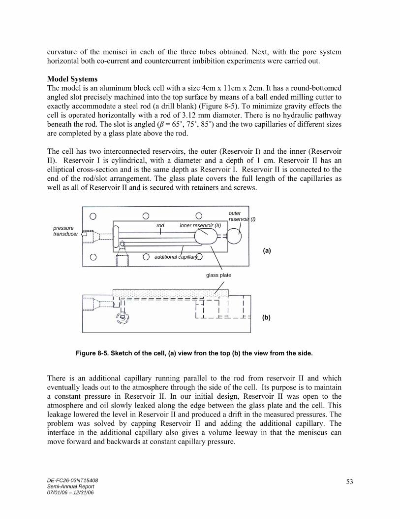
DE-FC26-03NT15408 Semi-Annual Report 07/01/06 – 12/31/06
53
curvature of the menisci in each of the three tubes obtained. Next, with the pore system horizontal both co-current and countercurrent imbibition experiments were carried out. Model Systems The model is an aluminum block cell with a size 4cm x 11cm x 2cm. It has a round-bottomed angled slot precisely machined into the top surface by means of a ball ended milling cutter to exactly accommodate a steel rod (a drill blank) (Figure 8-5). To minimize gravity effects the cell is operated horizontally with a rod of 3.12 mm diameter. There is no hydraulic pathway beneath the rod. The slot is angled (β = 65˚, 75˚, 85˚) and the two capillaries of different sizes are completed by a glass plate above the rod. The cell has two interconnected reservoirs, the outer (Reservoir I) and the inner (Reservoir II). Reservoir I is cylindrical, with a diameter and a depth of 1 cm. Reservoir II has an elliptical cross-section and is the same depth as Reservoir I. Reservoir II is connected to the end of the rod/slot arrangement. The glass plate covers the full length of the capillaries as well as all of Reservoir II and is secured with retainers and screws.
Figure 5. Sketch of the cell, (a) view from the top (b) the view from the side. There is an additional capillary running parallel to the rod from Reservoir II and which
Figure 8-5. Sketch of the cell, (a) view fron the top (b) the view from the side. There is an additional capillary running parallel to the rod from reservoir II and which eventually leads out to the atmosphere through the side of the cell. Its purpose is to maintain a constant pressure in Reservoir II. In our initial design, Reservoir II was open to the atmosphere and oil slowly leaked along the edge between the glass plate and the cell. This leakage lowered the level in Reservoir II and produced a drift in the measured pressures. The problem was solved by capping Reservoir II and adding the additional capillary. The interface in the additional capillary also gives a volume leeway in that the meniscus can move forward and backwards at constant capillary pressure.
rod inner reservoir
outer reservoir
Additional capillary
pressure transducer
rod inner reservoir (II)
outer reservoir (I)
glass plate
additional capillary (a)
(b)

DE-FC26-03NT15408 Semi-Annual Report 07/01/06 – 12/31/06
54
At the opposite end of the capillaries to Reservoir II there is a small chamber with a pressure tap for connection to one side of a sensitive differential pressure transducer (Furness Model FCO 44). The signal from the transducer is monitored by a data logger. A T-connection is placed where the additional capillary opens to the atmosphere. One end of this T-connection connects to one side of the differential pressure transducer and the other is connected to atmosphere via a long length of tubing. This design reduced the effects of short-term pressure changes in the room (i.e. doors opening). There is a slight depression ground into the glass plate just above the ends of the capillaries in Reservoir II which allows the bubbles formed during countercurrent imbibition to drift away after they have snapped off. Without this depression a successive bubble can fuse with its predecessor and trigger premature snap-off. Fluids For the imbibition experiments, both co-current and countercurrent, medicinal liquid paraffin was used to displace air. For the capillary rise experiments iso-octane was used . The densities of the liquids were measured using a pycnometer and the surface tensions using a surface tension balance (Model DB 2kS, White Electronics, WR, UK). The viscosity of paraffin was determined using a viscotester (ThermoHaake VT550, Haake, Germany). The properties of both liquids are given in Table 8-1.
Table 8-1. Properties of liquid paraffin and iso-octane. solution Density Viscosity surface
tension Liquid paraffin
0.83 g/cm3 180 mPa.s 33.83 dyne/cm
Iso-octane 0.71 g/cm3 ----- 19.42 dyne/cm
Meniscus curvatures When the rod touches the plate the system is basically a rod-in-an-angled-corner configuration for which the MS-P curvatures are known (Walsh, 1989). The capillary pressures for all of the menisci in the cells were measured by the capillary rise of iso-octane following the experimental procedure described by Mason and Morrow (1985). The actual capillary pressures for iso-octane and liquid paraffin are given in Table 8-2. Table 8-2. Capillary pressures (in Pa) determined by capillary rise experiments for iso-octane
(Iso.) and liquid paraffin (L.P.) in the rod-plate-contact cells. ∆P1 ∆P2 ∆Pa
Cell Iso. L.P. Iso. L.P. Iso. L.P.
Slot angle β 85º
133.60 232.53 105.62 183.78 31.52 54.85
Slot angle β 75º
165.18 287.41 80.22 139.61 27.62 48.32
Slot angle β 65º
212.26 368.92 64.71 112.59 27.48 47.80

DE-FC26-03NT15408 Semi-Annual Report 07/01/06 – 12/31/06
55
Normalized curvatures are compared with the MS-P theory in Figure 8-6.
0
4
8
12
16
20
24
50 70 90 110 130
slot angle
norm
aliz
ed c
urva
ture
MS-P
exp
incircle
Figure 8-6. Comparison of measured curvatures with values calculated by MS-P method for
the rod-in-angled corner geometry. Also shown is the incircle curvature (note that the insphere curvature would be double the incircle curvature).
Operation Before the experiment began, the correct volume of liquid paraffin (determined by trial) was placed in Reservoir I. The liquid was then pushed from Reservoir I by means of a close-fitting piston into Reservoir II. As the liquid is pushed out of Reservoir I, the oil level rises in Reservoir II and finally reaches the capillaries. Excess oil flows into the additional capillary forming a meniscus until it stops. In addition, a meniscus forms in each capillary on each side of the rod and these start to advance. For co-current imbibition, the pressure transducer is not connected to the cell. Hence, one end of the capillaries is open to the atmosphere. During countercurrent imbibition the transducer is connected and it measures the pressure build-up of the air in the dead end (∆Pd). For the interfaces in the two tubes there are arc menisci that advance along the corners forming liquid wedges. Although their curvature is high, their hydraulic resistance is also high (Dong and Chatzis, 1995). Consequently, as the main terminal menisci (Mason and Morrow, 1987) move along the capillaries the arc menisci do not advance far, nor carry much liquid, ahead of the main menisci.
Results Co-current imbibition Single frames from an experiment involving co-current flow are shown in Figure 8-7. The menisci have been drawn over for clarity.

DE-FC26-03NT15408 Semi-Annual Report 07/01/06 – 12/31/06
56
Figure 8-7. Single frames from an experiment involving co-current imbibition. Slot angle β is 75º.
Note that small meniscus is always ahead of the larger meniscus.
Equation 8-9 predicts that a plot of ( 2
0121 ,t, xx − ) vs ( 0tt − ) should be a straight line with the
gradient depending on the hydraulic resistance shape factor K. The same is true for the other capillary tube. Figure 8-8 shows the result for all three cells. The additional significance of the lines in Figure 8-8 being straight means that the capillary pressures generated by the menisci are constant, even though in each tube the velocity of advance varies considerably with time. The explanation is probably that the arc menisci in the corners always lead the main terminal meniscus. The significance is that in network models the interfaces are assumed to be quasi-static and generate a constant pressure. Figure 8-8 shows that this is probably a good approximation to the moving situation. In addition, Equation 8-10 predicts that a plot of 2
1x vs 22x is a straight line. This plot is
shown in Figure 8-9. It is interesting that the results for the 65º and 75º cells are almost coincident. This is because changes in the hydraulic resistance are almost compensated by changes in the capillary pressure. Because the capillaries have noncircular cross-sections with corners, their true hydraulic resistances are difficult to estimate (Dong and Chatzis, 1995; Ransohoff and Radke, 1998). This is why the shape factor, k, in Equation 8-7 is needed. For flow through circular tubes the average velocity, u , is given by Corey (1994)
xPr
dtdxu
µ8
2
== (8-24)
The shape factor k is 1/8 for this case. The hydraulic radius of irregular capillaries (rhyd) can be estimated from the ratio of the area to the perimeter (Corey, 1994; Sisavath et al., 2001; Patzek and Silin, 2001; Patzek and Kreistensen, 2001).
SArhyd = (8-25)
where A is the cross-sectional area perpendicular to flow, and S is the wetted perimeter. The A1, A2, S1 and S2 values are given in Equations 8-2 – 8-5.

DE-FC26-03NT15408 Semi-Annual Report 07/01/06 – 12/31/06
57
slot angle 65
0
200
400
600
800
1000
1200
0 10 20 30 40 50
t (s)
x2 (m
m2 )
small
large
slot angle 75
0
200
400
600
800
1000
1200
1400
0 20 40 60 80
t (s)
x2 (m
m2 )
small
large
slot angle 85
0
200
400
600
800
1000
1200
1400
1600
0 20 40 60 80 100
t (s)
x2 (m
m2 )
small
large
Figure 8-8. Plot of ( 2
02 xxt − ) vs ( 0tt − ) for both capillaries in each cell. Theory predicts that the
slope (m) should be equal to µ
KPPm
)(2 a∆−∆= values and the lines should be straight.

DE-FC26-03NT15408 Semi-Annual Report 07/01/06 – 12/31/06
58
0
200
400
600
800
1000
1200
1400
0 200 400 600 800 1000
x 12 (mm2)
x22
(mm
2 ) 65
75
85
Figure 8-9. Plot of 2
,1 tx vs. 2,2 tx for the cell with slot angles of 65º, 75º and 85º. Theory predicts
that the relationship should be straight lines.
Using distance-time measurements for each cell (and Equation 8-24) the hydraulic radius value for each capillary was found. The measured and theoretical values (from Equation 8-25) are compared in Figure 8-10. Good agreement was found between the experimental and the theoretical hydraulic radii values.
0
1
2
3
4
5
60 65 70 75 80 85 90
slot angle
r hyd
2/rhy
d1 theoryexp
Figure 8-10. Theoretical and experimental hydraulic radii value ratios at different slot angles
(º). ‘rhyd1’ is the hydraulic radius of the small capillary, ‘rhyd2’ is the hydraulic of the large capillary.
Countercurrent flow In counter- current imbibition, initially both interfaces advance, with the larger one leading. As the air is compressed, the large interface is pushed back by increasing air pressure until bubbles are blown from the large capillary tube. After each bubble snaps off, an interface advances a short way into the large capillary. Single frames from an experiment involving

DE-FC26-03NT15408 Semi-Annual Report 07/01/06 – 12/31/06
59
bubble snap-off during a countercurrent flow are shown in Figure 8-11. The menisci have been drawn over for clarity.
Figure 8-11. Countercurrent imbibition. A bubble is emerging from the large tube. After snap-off the meniscus invades the tube for some distance. Slot angle β is 75º.
At the beginning, before the oil is introduced into the capillaries, the differential pressure transducer shows a constant value of around 0 Pa. As the oil imbibes into the capillaries the pressure rises to the first positive peak. When the length of the large tube filled with oil decreases, the pressure drops slightly and then drops more rapidly as the bubble forms. Eventually the bubble snaps off and the air pressure rises back to almost the initial value and stays essentially constant until the next bubble starts to form. After the snap-off, the meniscus in the large tube appears to invade the tube for some distance but close observation shows that most of the liquid comes from drainage of the arc menisci until their curvature corresponds to that of the main meniscus. As the imbibition rate slows down, the time taken for bubble formation increases. This drop in rate is probably the cause of the slight increase in snap-off pressure of the later bubbles. With slower bubble growth the snap-off pressure moves closer to the curvature of a theoretical cylindrical meniscus within the tube. When the meniscus forms in the additional capillary, it creates an additional capillary pressure between the atmosphere and the fluid which, in effect, shifts the zero indicated pressure of the transducer. This pressure is equal to aP∆ and if this value is subtracted from the zero initial pressure, we obtain the ‘absolute base pressure’. The pressure produced by the additional capillary was obtained from the capillary rise experiments (see Table 8-2). The data plot for the transducer readings ( dP∆ ) of the cell with a slot angle of 85º is given in Figure 8-12.

DE-FC26-03NT15408 Semi-Annual Report 07/01/06 – 12/31/06
60
-100
-50
0
50
100
150
0 20 40 60 80 100 120 140 160 180
t (s)
Pd (
Pa)
Figure 8-12. Transducer pressure (∆Pd) recordings at the dead end in the cell during
countercurrent flow. The slot angle β is 85º. Negative peaks indicate bubble formation. Once the snap-off is completed, the air pressure regains the initial value and stays almost constant
until the next bubble starts to form.
In Figure 8-12, the negative peaks correspond to the onset of bubble formation. The bubble snaps off at the point ‘A’. Immediately after snap-off the pressure rises again as the arc menisci shrink back to the curvature of the main meniscus that now advances in the larger tube. This takes a surprisingly long time, mainly because of the considerable resistance to flow in the arc menisci. Little additional imbibition takes place during these local events which are mainly just a rearrangement of fluid. The time between sequential bubbles increases because advance of the meniscus in the smaller capillary slows with time. There are several measurements that can be made from the data pressure plot. The snap-off pressure is equal to the pressure between the absolute base pressure and the snap-off point ‘A’. The pressure difference created by the meniscus in the large tube (∆P2) is almost equal to the pressure difference between the absolute base pressure and the pressure that is measured between the formation of bubbles. When there is a constant capillary back pressure, the imbibition distance varies as t1/2, as predicted by the Washburn equation (Washburn, 1921) for cylindrical capillaries. However, when the bubble is forming the imbibition rate increases significantly. The imbibition distance ( 0xx − ) vs t1/2 for the small capillary during countercurrent flow is shown in Figure 8-13. Note that when a bubble starts to form, the imbibition rate increases and that after snap-off the t1/2 relationship is regained. The bumps on Figure 8-13 indicate bubble formation, the slope of the lines between bubble formation are almost the same. Comparison of Figure 12 with Figure 8-13 shows how the pressure change during bubble formation is matched by the increase in imbibition rate. The same data plots during countercurrent flow for the 75° and 65° cells are shown in Figures 8-14 – 8-17.
Snap-off pressure
∆P2
A
∆Pa
ABSOLUTE BASE
Bubble starts to form

DE-FC26-03NT15408 Semi-Annual Report 07/01/06 – 12/31/06
61
0
5
10
15
20
25
30
35
0 2 4 6 8 10 12 14 16 18
t 1/2
x- x
0
Figure 8-13. The rate of imbibition in the small capillary during countercurrent flow; slot angle β is 85º. The small steps accompany the formation of the bubbles. The dashed lines show that
the imbibition rate is almost the same between the bubble formation.
-60
-40
-20
0
20
40
60
80
100
120
0 20 40 60 80 100 120 140 160
t (s)
Pd (
Pa)
Figure 8-14. Pressure (∆Pd) recordings in the cell with a slot angle of 75º during
countercurrent flow.
A
ABSOLUTE BASE
Snap-off pressure
∆P2
∆Pa

DE-FC26-03NT15408 Semi-Annual Report 07/01/06 – 12/31/06
62
0
5
10
15
20
25
30
35
0 2 4 6 8 10 12 14 16 18 20
t 1/2
x-x
0
Figure 8-15. The rate of imbibition in the small capillary during countercurrent flow, slot angle
is 75º.
-60
-40
-20
0
20
40
60
80
0 20 40 60 80 100 120 140
t (s)
Pd (
Pa)
Figure 8-16. Pressure (∆Pd) recordings in the cell with a slot angle of 65º during
countercurrent flow.
∆P2
∆Pa Snap-off pressure
ABSOLUTE BASE
A

DE-FC26-03NT15408 Semi-Annual Report 07/01/06 – 12/31/06
63
0
5
10
15
20
25
30
35
40
0 2 4 6 8 10 12 14 16 18
t 1/2
x-x
0
Figure 8-17. The imbibition rate in the small capillary during countercurrent flow; slot angle is
65º. Only one bubble was formed because of the small tube contained so little volume. The snap-off pressure can be estimated from the incircle that just fits inside the tube (see Figure 8-2). For the 85º cell, the incircle normalized curvature under the condition ‘d/R=0’ is 5.16. Capillary pressure is related to curvature by
∆P = σ C/R (8-26) where ∆P is the capillary pressure, σ is the surface tension, C is the normalized curvature and R is the rod radius. From the incircle, the capillary pressure is calculated as 109 Pa. However, from the graph, the actual pressure for the first bubble is 70 Pa (Figure 8-12). The difference is probably because flow needs to occur for snap-off and a pressure is needed to drive this flow. The pressure at which snap- off occurs therefore depends upon the rate at which the bubble is growing, and this, in turn, depends on the position of the meniscus in the small tube. The effect can be seen in Figure 8-12 where the later bubbles snap off at higher pressures. The snap-off pressure therefore exhibits rate-dependency under dynamic conditions. In addition, the interface is not a perfect uniform cylinder. The measured curvatures are compared with the curvatures obtained from the incircle curvatures in Figure 8-18. The pressure produced by the meniscus in the large tube (∆P2 ) can be measured from the pressure record during flow. The values for all three cells can be compared with the capillary pressures obtained using capillary rise values (Table 8-2) and using Equation 8-26, where the normalized curvatures are from the MS-P theory (Figure 8-2). It can be seen that they are in excellent agreement (Figure 8-19) indicating that flow does not greatly affect the meniscus curvature predicted by the MS-P theory. To our best knowledge this has not been reported previously in other papers.

DE-FC26-03NT15408 Semi-Annual Report 07/01/06 – 12/31/06
64
0
1
2
3
4
5
6
7
60 65 70 75 80 85 90
slot angle
norm
aliz
ed c
urva
ture
incircleexp
Figure 8-18. Comparison of incircle curvature with snap-off curvature. The snap-off pressures were read from Figures 12, 14 and 16 for the slot angles of 85º (3 bubbles), 75º (2 bubbles) and
65º (1 bubble), respectively.
0
40
80
120
160
200
60 65 70 75 80 85 90
slot angle
P2 (
Pa) cap rise
flowMS-P
Figure 8-19. Theoretical MS-P and experimental (capillary rise and flow) ∆P2 values at different
slot angles (º). Equation 8-19 gives the pressure difference between atmosphere and the dead end (∆Pd) for the constant pressure periods between the release and formation of bubbles. The ∆Pd values were measured as 72 Pa, 90 Pa and 120 Pa for the cells with slot angles 65º, 75º, and 85º respectively (see Figures 8-12, 8-14 and 8-16). Corresponding pressure values from Equation 8-19 are 75 Pa, 103 Pa and 130 Pa. The countercurrent theory presented here only considers the regions between consecutive bubbles, and does not analyze behavior during bubble formation. Equation 8-20 predicts interface positions during countercurrent imbibition without a bubble being formed. In one series of experiments, imbibition was initially co-current and then the

DE-FC26-03NT15408 Semi-Annual Report 07/01/06 – 12/31/06
65
end was sealed and the imbibition became countercurrent. The B coefficient values were calculated from co-current measurements for all three cells 65º, 75º and 85º as 0.015, 0.078 and 0.35 respectively, while x1 and x2 values were determined from the countercurrent video images. Values for A1 and A2 were calculated using Equations 8-2 and 8-3, respectively. Following Equation 8-23, ( )2
221 , xxf vs time were plotted. As expected an almost linear
relationship for each cell was obtained (Figure 8-20).
-70
-60
-50
-40
-30
-20
-10
00 20 40 60 80 100 120 140
t (s)
f(x
12 , x22 ) 65
75
85
Figure 8-20. Relationship between function of ( )22
21 , xxf versus time during countercurrent
flow for cell with slot angles of 65º, 75º and 85º.
References Cil, M., J.C. Reis, J. Petroleum Sci. Eng. 16 (1996) 61. Corey, A.T., Mechanics of Immiscible Fluids in Porous Media, Water Resources Publications,
Colorado, 1994. Dong, M., F.A.L. Dullien, Transp. Porous Media. 27 (1997) 185. Dong, M., F.A.L. Dullien, J.Zhou, Transp. Porous Media, 31 (1998) 213. Dong, M., I. Chatzis, J. Colloid Interface Sci. 172 (1995) 278. Dong, M., F.A.L. Dullien, L. Dai, D. Li, Transp. Porous Media. 59 (2005) 1. Dong, M., F.A.L. Dullien, L. Dai, D. Li, Transp. Porous Media. 63, (2006) 289. Dullien, F.A.L., in: V. Kambiz (Eds), Handbook of Porous Media Marcel Dekker, Inc., New
York, 2000, p. 53. Lenormand, R., R., E. Toubul, C. Zarcone, J. Fluid Mech. 189 (1988) 165. Li, Y., N.R. Morrow, D. Ruth, J. Petroleum Sci. Eng. 39 (2003) 309. Ma, S., G. Mason, N.R. Morrow, Colloids and Surfaces A: Physicochemical and Engineering
Aspects. 117 (1996) 273. Mason, G., Chem. Eng. J. 38 (1983) 1455. Mason, G., N.R. Morrow, J. Chem. Soc. Faraday Trans. 80 (1984) 2375. Mason, G., N.R. Morrow, J. Colloid Interface Sci. 109 (1985) 46. Mason, G., N.R. Morrow, Proc. R. Soc. London A. 414 (1987) 111.
DE-FC26-03NT15408 Semi-Annual Report 07/01/06 – 12/31/06
66
Mason, G., N.R. Morrow, T.J. Walsh, Studies Surface Sci. Catalysis. 128 (2000) 495. Mayer, R.P., R.A. Stowe, J. Colloid Interface Sci. 20 (1965) 893. Nicholson, D., J.H. Petropoulos, J. Physics D: Applied Physics. 4 (1971) 181. Nicholson, D., J.H. Petropoulos, J. Physics D: Applied Physics. 6 (1973) 1737. Princen, H.M., J. Colloid Interface Sci. 30 (1969a) 69. Princen, H.M., J. Colloid Interface Sci. 30 (1969b) 359. Princen, H.M., J. Colloid Interface Sci. 34 (1970) 171. Patzek, T.W., J.G. Kristensen, J. Colloid Interface Sci. 236 (2001) 305. Patzek, T.W., D.B. Silin, J. Colloid Interface Sci. 236 (2001) 295. Ransohoff, T.C., C.J. Radke, J. Colloid Interface Sci. 172 (1988) 178. Reis, J.C., M. Cil, J. Petroleum Sci. Eng. 10 (1993) 97. Ruth, D., J.T. Bartley, J. Proc. 2002 International Symposium of the Society of Core Analysts,
Monterey, California, SCA2002-05, (2003) 12. Sisavath, S., X. Jing, R.W, Zimmerman, Transp. Porous Media. 45 (2001) 41. Washburn, E.W., The Physical Review. 17 (1921) 273. Walsh, T.J., “Capillary properties of model pores”. PhD Thesis, Loughborough University of
Technology, 1989.
Task 9. Increased oil recovery by spontaneous imbibition. The methods described under Task 6 are now being adapted to measure the buble pressures for oil production. The effect of reduction of bubble pressure on oil production rate by means of surfactants and other controlled methods of lowering interfacial tension will be tested. Further tests and variation of brine composition on use of surfactants to improve oil recovery are in progress.
CONCLUSIONS
Task 6 • Pressures in the oil phase ahead of the imbibition front (end pressures) for restricted
countercurrent spontaneous imbibition have been determined for a range of conditions. These novel measurements include strongly water wet cores with and without initial water saturation, mixed wet cores with different levels of initial water saturation, and cores initially saturated with crude oil.
• Strongly water wet cores showed decrease in end pressure with increase in initial water
saturation consistent with decrease in the capillary driving force. • In contrast to water wet conditions, mixed wet cores showed increase in driving pressure
with increase in initial water saturation. This result is consistent with the effect of aging on the available surface energy for imbibition and with standard imbibition tests on mixed wet rocks having a range of initial water saturations.
• Measured pressures stayed close to constant until the imbibition front reached the end of the
core sample.
DE-FC26-03NT15408 Semi-Annual Report 07/01/06 – 12/31/06
67
Task 7
• An analytic solution for imbibition has been developed by approximating the countercurrent imbibition process to a frontal displacement with constant saturations ahead of and behind the front, and taking the capillary back pressure at the open face to be a constant fraction of the capillary pressure at the front. This gives the production vs time functions for different core shapes. Comparison of these functions with experimental data using Berea sandstone and refined oil for both the linear and radial cases shows reasonable agreement. Variability between the cores caused by not having enough surface area and not enough volume seems of greater importance than the precise core scale factor functions.
Task 8.
• A simple analysis of co- and countercurrent imbibition for tubes of non-circular cross- section has been carried out. Shape factors were needed to describe the tube areas, hydraulic resistances and capillary pressures. Experiments using model pore systems and measurements of capillary rise were used to confirm the capillary pressures. Co-current imbibition experiments were used to measure the hydraulic resistances. Both these values were then used to quantify countercurrent imbibition. When theory was compared to experiment, the agreement was generally good
• In general, co-current imbibition was observed to occur at about four times the rate of
countercurrent imbibition. Furthermore, it takes a significant positive pressure, the capillary back pressure, for air to be driven out in countercurrent imbibition and this can make a significant difference to the imbibition rate. At the liquid inlet face there was growth of bubbles and subsequent snap-off giving significant fluctuations of the capillary back pressure. Co-current theory was in good agreement with the experiments.
• The Mayor & Stowe –Princen theory appears to predict meniscus curvatures well, even
when they are moving. This is probably because the arc menisci keep far enough ahead of the main terminal meniscus for the MS-P approximations to hold.