Embed Size (px)
Citation preview
Noboru Takigawa · Kouhei Washiyama
Fundamentals of Nuclear Physics
Fundamentals of Nuclear Physics
Noboru Takigawa • Kouhei Washiyama
Fundamentals of NuclearPhysics
123
Noboru TakigawaDepartment of PhysicsGraduate School of ScienceTohoku UniversitySendaiJapan
Kouhei WashiyamaCenter for Computational SciencesUniversity of TsukubaTsukuba, IbarakiJapan
ISBN 978-4-431-55377-9 ISBN 978-4-431-55378-6 (eBook)DOI 10.1007/978-4-431-55378-6
Library of Congress Control Number: 2016958483
Translation from the Japanese language edition: Genshikaku Butsurigaku by Noboru Takigawa, ©Asakura Publishing Company, Ltd. 2013. All rights reserved.© Springer Japan 2017This work is subject to copyright. All rights are reserved by the Publisher, whether the whole or partof the material is concerned, specifically the rights of translation, reprinting, reuse of illustrations,recitation, broadcasting, reproduction on microfilms or in any other physical way, and transmissionor information storage and retrieval, electronic adaptation, computer software, or by similar or dissimilarmethodology now known or hereafter developed.The use of general descriptive names, registered names, trademarks, service marks, etc. in thispublication does not imply, even in the absence of a specific statement, that such names are exempt fromthe relevant protective laws and regulations and therefore free for general use.The publisher, the authors and the editors are safe to assume that the advice and information in thisbook are believed to be true and accurate at the date of publication. Neither the publisher nor theauthors or the editors give a warranty, express or implied, with respect to the material contained herein orfor any errors or omissions that may have been made.
Printed on acid-free paper
This Springer imprint is published by Springer NatureThe registered company is Springer Japan KKThe registered company address is: Chiyoda First Bldg. East, 3-8-1 Nishi-Kanda, Chiyoda-ku,Tokyo 101-0065, Japan
To Noriko, Akiko, Tsuyoshiand to our parents.
Preface
This book provides an introduction to nuclear physics. Research in nuclear physicscovers a wide variety of subjects, and one can list many key words: nuclearstructure and reactions of stable and unstable nuclei, fission and decay of a nucleus,extreme states such as the limits of existence and high-spin states, properties at hightemperature and high density, hypernuclei, neutron stars, and nucleosynthesis,among others. All of these are the subjects of nuclear physics. In addition to theserather static properties, nuclear reactions such as heavy-ion collisions introduce newaspects of research, i.e., dynamical properties of nuclei or reaction mechanisms,such as heavy-ion fusion reactions, dissipation phenomena and liquid–gas phasetransition. Many of these phenomena can be understood from the point of view thata nucleus is a quantum many-body system of nucleons stabilized by nuclear force.On the other hand, phenomena at higher energies, driven by, e.g., high-energyheavy-ion collisions, require a different approach: the approach based on thequantum chromodynamics (QCD). The study of quark–gluon plasma and of theQCD phase diagram is representative and forms a large stream of current nuclearphysics.
In this book, we largely restrict our subjects and describe basic features ofnuclear structure and of nuclear decays. b-decay and most excitation motions areleft to other books. Also, nuclear reactions and current subjects such as physics ofunstable nuclei, hypernuclei, and nuclear physics based on QCD are untouchedexcept for occasional very brief references. Even with these limitations, we couldonly briefly mention recent developments. However, we have tried to convey partof them through columns on the QCD phase diagram of nuclear matter, superheavyelements, superdeformed states, and overview of the synthesis of elements. Wehope that together with the main text they help readers to grasp our currentknowledge of the nucleus and some recent research trends in nuclear physics. Byrestricting the subjects, our aim was to contain many experimental data of basicnuclear properties or suitable illustrations and explain the main structural features ofnuclei in some detail. This will be useful because most of the phenomena listed inthe first paragraph, but omitted from the book, are intimately related to thosebasic properties. We also have attempted to explain how the nuclear model has
vii
developed from the original phenomenological level of a shell model to the modernunderstanding based on a many-body theory such as the Hartree–Fock calculations.We also have described nuclear force, the basis of nuclear physics, in some detail.We sometimes introduce semi-classical approximation to the original quantummechanical formalism. We hope that it helps the readers to intuitively grasp theunderlying physics of complicated nuclear phenomena.
In writing the book our intention was to create not only a good introduction tonuclear physics, but also a good reference book for physicists to learn the appli-cation of quantum mechanics and mathematics. Toward that aim, in addition todescribing the basic phenomena of a nucleus, we attempted to convey how the basicsubjects of modern physics such as quantum mechanics, statistical physics, math-ematics for physics, e.g., complex integrals, are used to describe or interpret variousphenomena of nucleus. We also considered the standard level of knowledge ofjunior and senior students, and gave a detailed description to enable them to deriveeach equation. Finally, we added the appendix to prove a number of importantformulae in the main text and to show some fundamental formulae.
The contents of the book are based on the lectures that one of the authors, N.T.,has delivered at Tohoku University, Sendai, Japan, for a long time to junior andsenior students in the undergraduate physics course and also to beginning graduatestudents. We have included as sidebars some additional material that was presentedin the class in order to keep the atmosphere of the lecture. Many textbooks andoriginal papers and figures therein have helped in preparing the lectures and thisbook. Several of the figures are taken from them. Using this opportunity, we wish tothank the authors. The papers cited at various places are not at all complete.Moreover, it does not mean that they are necessarily the representative papers oneach citation. Nevertheless, we hope that they can help readers to do further study.This book is an English translation of the Japanese edition, which one of theauthors, N.T., published in 2013. The appendix contains the errata to the originalJapanese edition.
We would like to thank Akif Baha Balantekin for many useful comments for thewriting of this English edition. We thank D.M. Brink, A.B. Balantekin, N. Rowley,F. Michel, S.Y. Lee, P. Fröbrich, S. Landowne, K. McVoy, W.A. Friedman,G.F. Bertsch, A. Brown, H. Weidenmüller, H. Friedrich, H. Esbensen,M.S. Hussein, L.F. Canto, C. Bertulani, P.R.S. Gomes, D. Hinde, M. Dasgupta,G. Pollarolo, A. Bonasera, M. Di Toro, C. Spitaleri, C. Rolfs, I. Thompson,S. Ayik, K. Hara, Y. Abe, H. Sagawa, A. Iwamoto, T. Tazawa, M. Ohta, J. Kasagi,and many other colleagues and friends around the world; and K. Hagino andA. Ono in the Nuclear Theory Group of Tohoku University, Sendai, for usefuldiscussions. We are grateful to students of Tohoku University, especially foreignstudents, for stimulating us to write this English book. We would like to thankF. Minato, S. Yusa, S. Iwasaki and his wife, H. Tamura, and H. Koura for preparingfigures, and K. Morita, T. Hirano, Y. Aritomo, T. Kajino, and Y. Motizuki inpreparing the columns; and P. Möller, T. Wada, K. Matsuyanagi, T. Tamae, andK. Kato for kindly reading sections of the Japanese edition and making manyhelpful suggestions. We also thank all the mentors and collaborators who provided
viii Preface

us opportunities to work in their institutions. We are grateful to H. Niko andR. Takizawa for their help as the editors of this English version. Above allN.T. would like to thank his wife, Noriko, and his family for their support over theyears.
Sendai, Japan Noboru TakigawaSeptember 2016 Kouhei Washiyama
Preface ix
Contents
1 Introduction . . . . . . . . . . . . . . . . . . . . . . . . . . . . . . . . . . . . . . . . . . . . . . 11.1 The Constituents and Basic Structure of Atomic Nuclei . . . . . . . . . 11.2 Properties of Particles Relevant to Nuclear Physics . . . . . . . . . . . . 21.3 The Role of Various Forces . . . . . . . . . . . . . . . . . . . . . . . . . . . . . . 61.4 Useful Physical Quantities . . . . . . . . . . . . . . . . . . . . . . . . . . . . . . . 71.5 Species of Nuclei . . . . . . . . . . . . . . . . . . . . . . . . . . . . . . . . . . . . . . 81.6 Column: QCD Phase Diagram of Nuclear Matter . . . . . . . . . . . . . . 11References. . . . . . . . . . . . . . . . . . . . . . . . . . . . . . . . . . . . . . . . . . . . . . . . 12
2 Bulk Properties of Nuclei . . . . . . . . . . . . . . . . . . . . . . . . . . . . . . . . . . . 132.1 Nuclear Sizes . . . . . . . . . . . . . . . . . . . . . . . . . . . . . . . . . . . . . . . . . 13
2.1.1 Rutherford Scattering . . . . . . . . . . . . . . . . . . . . . . . . . . . . . 132.1.2 Electron Scattering . . . . . . . . . . . . . . . . . . . . . . . . . . . . . . . 172.1.3 Mass Distribution . . . . . . . . . . . . . . . . . . . . . . . . . . . . . . . . 25
2.2 Number Density and Fermi Momentum of Nucleons . . . . . . . . . . . 282.2.1 Number Density of Nucleons . . . . . . . . . . . . . . . . . . . . . . . 282.2.2 Fermi Momentum: Fermi-Gas Model, Thomas–Fermi
Approximation . . . . . . . . . . . . . . . . . . . . . . . . . . . . . . . . . . 282.3 Nuclear Masses. . . . . . . . . . . . . . . . . . . . . . . . . . . . . . . . . . . . . . . . 31
2.3.1 The Binding Energies: Experimental Data andCharacteristics . . . . . . . . . . . . . . . . . . . . . . . . . . . . . . . . . . . 32
2.3.2 The Semi-empirical Mass Formula (The Weizsäcker–Bethe Mass Formula)—The Liquid-Drop Model. . . . . . . . . 42
2.3.3 Applications of the Mass Formula (1): The Stability Line,the Heisenberg Valley . . . . . . . . . . . . . . . . . . . . . . . . . . . . . 43
2.3.4 Applications of the Mass Formula (2): Stabilitywith Respect to Fission . . . . . . . . . . . . . . . . . . . . . . . . . . . . 46
2.3.5 Application to Nuclear Power Generation . . . . . . . . . . . . . . 572.3.6 Fission Isomers . . . . . . . . . . . . . . . . . . . . . . . . . . . . . . . . . . 60
References. . . . . . . . . . . . . . . . . . . . . . . . . . . . . . . . . . . . . . . . . . . . . . . . 64
xi
3 The Nuclear Force and Two-Body Systems . . . . . . . . . . . . . . . . . . . . . 653.1 The Fundamentals of Nuclear Force . . . . . . . . . . . . . . . . . . . . . . . . 65
3.1.1 The Range of Forces—A Simple Estimateby the Uncertainty Principle . . . . . . . . . . . . . . . . . . . . . . . . 65
3.1.2 The Radial Dependence . . . . . . . . . . . . . . . . . . . . . . . . . . . 663.1.3 The State Dependence of Nuclear Force . . . . . . . . . . . . . . . 67
3.2 The General Structure of Nuclear Force . . . . . . . . . . . . . . . . . . . . . 713.2.1 Static Potentials (Velocity-Independent Potentials) . . . . . . . 713.2.2 Velocity-Dependent Potentials. . . . . . . . . . . . . . . . . . . . . . . 73
3.3 The Properties of Deuteron and the Nuclear Force . . . . . . . . . . . . . 743.3.1 The Effect of Tensor Force: The Wave Function
in the Spin–Isospin Space . . . . . . . . . . . . . . . . . . . . . . . . . . 743.3.2 The Radial Wave Function: Estimate of the Magnitude
of the Force Between Proton and Neutron . . . . . . . . . . . . . 773.4 Nucleon–Nucleon Scattering. . . . . . . . . . . . . . . . . . . . . . . . . . . . . . 78
3.4.1 Low-Energy Scattering: Effective Range Theory. . . . . . . . . 783.4.2 High-Energy Scattering: Exchange Force . . . . . . . . . . . . . . 813.4.3 High-Energy Scattering: Repulsive Core . . . . . . . . . . . . . . . 833.4.4 Spin Polarization Experiments. . . . . . . . . . . . . . . . . . . . . . . 85
3.5 Microscopic Considerations: Meson Theory, QCD. . . . . . . . . . . . . 853.6 Phenomenological Potential with High Accuracy: Realistic
Potential . . . . . . . . . . . . . . . . . . . . . . . . . . . . . . . . . . . . . . . . . . . . . 883.6.1 Hamada–Johnston Potential. . . . . . . . . . . . . . . . . . . . . . . . . 893.6.2 Reid Potential . . . . . . . . . . . . . . . . . . . . . . . . . . . . . . . . . . . 91
3.7 Summary of the Nuclear Force in the Free Space . . . . . . . . . . . . . 913.8 Effective Interaction Inside Nucleus . . . . . . . . . . . . . . . . . . . . . . . . 92
3.8.1 G-Matrix . . . . . . . . . . . . . . . . . . . . . . . . . . . . . . . . . . . . . . . 923.8.2 Phenomenological Effective Interaction. . . . . . . . . . . . . . . . 94
References. . . . . . . . . . . . . . . . . . . . . . . . . . . . . . . . . . . . . . . . . . . . . . . . 96
4 Interaction with Electromagnetic Field:Electromagnetic Moments. . . . . . . . . . . . . . . . . . . . . . . . . . . . . . . . . . . 974.1 Hamiltonian of the Electromagnetic Interaction
and Electromagnetic Multipole Moments . . . . . . . . . . . . . . . . . . . . 974.1.1 Operators for the Dipole and Quadrupole Moments . . . . . . 984.1.2 Various Corrections. . . . . . . . . . . . . . . . . . . . . . . . . . . . . . . 1004.1.3 Measurement of the Magnetic Moment: Hyperfine
Structure . . . . . . . . . . . . . . . . . . . . . . . . . . . . . . . . . . . . . . . 1004.2 Electromagnetic Multipole Operators . . . . . . . . . . . . . . . . . . . . . . . 1024.3 Properties of the Electromagnetic Multipole Operators . . . . . . . . . . 103
4.3.1 Parity, Tensor Property and Selection Rule . . . . . . . . . . . . . 1034.3.2 Definition of the Electromagnetic Moments . . . . . . . . . . . . 104
References. . . . . . . . . . . . . . . . . . . . . . . . . . . . . . . . . . . . . . . . . . . . . . . . 106
xii Contents
5 Shell Structure . . . . . . . . . . . . . . . . . . . . . . . . . . . . . . . . . . . . . . . . . . . . 1075.1 Magic Numbers . . . . . . . . . . . . . . . . . . . . . . . . . . . . . . . . . . . . . . . 1075.2 Explanation of the Magic Numbers by Mean-Field Theory . . . . . . 109
5.2.1 The Mean Field. . . . . . . . . . . . . . . . . . . . . . . . . . . . . . . . . . 1095.2.2 Energy Levels for the Infinite Square-Well Potential . . . . . 1105.2.3 The Harmonic Oscillator Model . . . . . . . . . . . . . . . . . . . . . 1115.2.4 The Magic Numbers in the Static Potential Due
to Short Range Force . . . . . . . . . . . . . . . . . . . . . . . . . . . . . 1125.2.5 Spin–Orbit Interaction . . . . . . . . . . . . . . . . . . . . . . . . . . . . . 114
5.3 The Spin and Parity of the Ground and Low-Lying Statesof Doubly-Magic �1 Nuclei. . . . . . . . . . . . . . . . . . . . . . . . . . . . . . 117
5.4 The Magnetic Dipole Moment in the Ground State of OddNuclei: Single Particle Model . . . . . . . . . . . . . . . . . . . . . . . . . . . . . 1195.4.1 The Schmidt Lines . . . . . . . . . . . . . . . . . . . . . . . . . . . . . . . 1205.4.2 Configuration Mixing and Core Polarization . . . . . . . . . . . . 1215.4.3 [Addendum] The Anomalous Magnetic Moments
of Nucleons in the Quark Model. . . . . . . . . . . . . . . . . . . . . 1235.5 Mass Number Dependence of the Level Spacing �hx . . . . . . . . . . . 1245.6 The Magnitude and Origin of Spin–Orbit Interaction . . . . . . . . . . . 1255.7 Difference Between the Potentials for Protons
and for Neutrons: Lane Potential . . . . . . . . . . . . . . . . . . . . . . . . . . 1255.8 The Spin and Parity of Low-Lying States
of Doubly-Magic �2 Nuclei and the Pairing Correlation . . . . . . . . 1275.8.1 The Spin and Parity of the Ground and Low Excited
States of 21082 Pb. . . . . . . . . . . . . . . . . . . . . . . . . . . . . . . . . . . 127
5.8.2 The Effect of d-Type Residual Interaction: PairingCorrelation . . . . . . . . . . . . . . . . . . . . . . . . . . . . . . . . . . . . . 128
5.9 Column: Superheavy Elements (SHE) . . . . . . . . . . . . . . . . . . . . . . 130References. . . . . . . . . . . . . . . . . . . . . . . . . . . . . . . . . . . . . . . . . . . . . . . . 133
6 Microscopic Mean-Field Theory (Hartree–Fock Theory) . . . . . . . . . . 1356.1 Hartree–Fock Equation . . . . . . . . . . . . . . . . . . . . . . . . . . . . . . . . . . 135
6.1.1 Equivalent Local Potential, Effective Mass . . . . . . . . . . . . . 1366.1.2 Nuclear Matter and Local Density Approximation . . . . . . . 1376.1.3 Saturation Property in the Well-Behaved Potential,
Constraint to the Exchange Property . . . . . . . . . . . . . . . . . . 1406.2 Skyrme Hartree–Fock Calculations for Finite Nuclei . . . . . . . . . . . 141
6.2.1 Skyrme Force . . . . . . . . . . . . . . . . . . . . . . . . . . . . . . . . . . . 1416.2.2 Skyrme Hartree–Fock Equation. . . . . . . . . . . . . . . . . . . . . . 1436.2.3 Energy Density and Determination of Parameters . . . . . . . . 1446.2.4 Comparison with the Experimental Data . . . . . . . . . . . . . . . 1476.2.5 The Equation of State, Saturation, Spinodal Line,
Surface Thickness . . . . . . . . . . . . . . . . . . . . . . . . . . . . . . . . 1486.2.6 Beyond the Hartree–Fock Calculations:
Nucleon–Vibration Coupling; x-Mass . . . . . . . . . . . . . . . . 154
Contents xiii
6.3 Relativistic Mean-Field Theory (rxq Model). . . . . . . . . . . . . . . . . 1556.3.1 Lagrangian . . . . . . . . . . . . . . . . . . . . . . . . . . . . . . . . . . . . . 1566.3.2 Field Equations . . . . . . . . . . . . . . . . . . . . . . . . . . . . . . . . . . 1576.3.3 The Mean-Field Theory . . . . . . . . . . . . . . . . . . . . . . . . . . . 1586.3.4 Prologue to How to Solve the Mean-Field Equations . . . . . 1586.3.5 Non-relativistic Approximation and the Spin–Orbit
Coupling . . . . . . . . . . . . . . . . . . . . . . . . . . . . . . . . . . . . . . . 1606.3.6 Parameter Sets. . . . . . . . . . . . . . . . . . . . . . . . . . . . . . . . . . . 161
6.4 Pairing Correlation . . . . . . . . . . . . . . . . . . . . . . . . . . . . . . . . . . . . . 1626.4.1 Overview . . . . . . . . . . . . . . . . . . . . . . . . . . . . . . . . . . . . . . 1626.4.2 Multipole Expansion of the Pairing Correlation,
Monopole Pairing Correlation Model and Quasi-SpinFormalism . . . . . . . . . . . . . . . . . . . . . . . . . . . . . . . . . . . . . . 163
6.4.3 BCS Theory . . . . . . . . . . . . . . . . . . . . . . . . . . . . . . . . . . . . 1646.4.4 The Magnitude of the Gap Parameter . . . . . . . . . . . . . . . . . 1686.4.5 The Coherence Length . . . . . . . . . . . . . . . . . . . . . . . . . . . . 169
References. . . . . . . . . . . . . . . . . . . . . . . . . . . . . . . . . . . . . . . . . . . . . . . . 170
7 The Shapes of Nuclei. . . . . . . . . . . . . . . . . . . . . . . . . . . . . . . . . . . . . . . 1717.1 The Observables Relevant to the Nuclear Shape: Multipole
Moments and the Excitation Spectrum . . . . . . . . . . . . . . . . . . . . . . 1717.2 Deformation Parameters . . . . . . . . . . . . . . . . . . . . . . . . . . . . . . . . . 1747.3 The Deformed Shell Model . . . . . . . . . . . . . . . . . . . . . . . . . . . . . . 1777.4 Nucleon Energy Levels in a Deformed One-Body Field:
Nilsson Levels . . . . . . . . . . . . . . . . . . . . . . . . . . . . . . . . . . . . . . . . 1807.5 The Spin and Parity of the Ground State of Deformed
Odd Nuclei . . . . . . . . . . . . . . . . . . . . . . . . . . . . . . . . . . . . . . . . . . . 1827.6 Theoretical Prediction of Nuclear Shape. . . . . . . . . . . . . . . . . . . . . 182
7.6.1 The Strutinsky Method: Macroscopic–MicroscopicMethod . . . . . . . . . . . . . . . . . . . . . . . . . . . . . . . . . . . . . . . . 182
7.6.2 Constrained Hartree–Fock Calculations . . . . . . . . . . . . . . . . 1847.7 Column: Superdeformed States. . . . . . . . . . . . . . . . . . . . . . . . . . . . 187References. . . . . . . . . . . . . . . . . . . . . . . . . . . . . . . . . . . . . . . . . . . . . . . . 188
8 Nuclear Decay and Radioactivity . . . . . . . . . . . . . . . . . . . . . . . . . . . . . 1918.1 Alpha Decay. . . . . . . . . . . . . . . . . . . . . . . . . . . . . . . . . . . . . . . . . . 191
8.1.1 Decay Width . . . . . . . . . . . . . . . . . . . . . . . . . . . . . . . . . . . . 1928.1.2 The Geiger–Nuttal Rule . . . . . . . . . . . . . . . . . . . . . . . . . . . 200
8.2 Fission . . . . . . . . . . . . . . . . . . . . . . . . . . . . . . . . . . . . . . . . . . . . . . 2008.3 Electromagnetic Transitions . . . . . . . . . . . . . . . . . . . . . . . . . . . . . . 203
8.3.1 Multipole Transition, Reduced Transition Probability . . . . . 2038.3.2 General Consideration of the Selection Rule
and the Magnitude . . . . . . . . . . . . . . . . . . . . . . . . . . . . . . . 2058.3.3 Single-Particle Model Estimate: Weisskopf Units
and Experimental Values. . . . . . . . . . . . . . . . . . . . . . . . . . . 206
xiv Contents
8.3.4 Connection Between Electromagnetic Transitionsand the Shapes and Collective Motions of Nuclei . . . . . . . . 209
References. . . . . . . . . . . . . . . . . . . . . . . . . . . . . . . . . . . . . . . . . . . . . . . . 212
9 Synthesis of Elements . . . . . . . . . . . . . . . . . . . . . . . . . . . . . . . . . . . . . . 2159.1 The Astrophysical S-Factor and Gamow Factor . . . . . . . . . . . . . . . 2159.2 Gamow Peak . . . . . . . . . . . . . . . . . . . . . . . . . . . . . . . . . . . . . . . . . 2179.3 Neutron Capture Cross Section. . . . . . . . . . . . . . . . . . . . . . . . . . . . 2189.4 Synthesis of Heavy Elements: S-Process and R-Process . . . . . . . . . 2199.5 Column: Overview of the Synthesis of Elements . . . . . . . . . . . . . . 220References. . . . . . . . . . . . . . . . . . . . . . . . . . . . . . . . . . . . . . . . . . . . . . . . 221
Appendix A: Important Formulae and Their Derivation . . . . . . . . . . . . . 223
Index . . . . . . . . . . . . . . . . . . . . . . . . . . . . . . . . . . . . . . . . . . . . . . . . . . . . . . 261
Contents xv
Chapter 1Introduction
Abstract It would be useful to have an overview of some fundamental aspects ofnuclei before discussing each subject in detail. In this connection, we briefly describein this chapter the constituents and basic structure of atomic nuclei, properties ofparticles which are closely related to nuclear physics, the role of the four fundamentalforces in nature in nuclear physics, nuclear species, the abundance of elements andthe phase diagram of nuclear matter.
1.1 The Constituents and Basic Structure of Atomic Nuclei
The atomic nuclei are self-bound many-body systems of protons (p) and neutrons (n)by strong interaction. Although other baryons such as Δ(1232) are also contained,their amounts are small. For example, the percentage of Δ(1232)Δ(1232) containedin the lightest nucleus deuteron (d) is about 1%.π -mesons in virtual statesmediate theinteraction between the constituent particles and affect the electromagnetic propertiesof protons and neutrons. Furthermore, each proton and neutron is also a compositeparticle consisting of three quarks. The other hadrons also consist of quarks. One cantherefore take also the view that atomic nuclei are many-body systems of quarks.
The picture of nuclei and of nuclear phenomena, hence the appropriate way todescribe them, depend on the object and method of observation and the relatedenergy scale, and lead to various models for nuclei. This book restricts to low-energy phenomena and discusses the nuclear structure and properties primarily fromthe point of view that nuclei are many-body systems of protons and neutrons. Thegoverning law is quantum mechanics. This contrasts to quantum chromodynamicsfor high-energy phenomena. Among various quantum many-body systems, nucleihave characteristics that the number of constituents is small and also that the leadingforces are strong interactions.
Each nucleus is represented, for example, as 168O. O is the symbol of the chemical
element. It represents oxygen in this example, hence the number of protons is 8.This number is called the atomic number, and is given at the left lower side. It isoften omitted, because it has a one to one correspondence to the symbol of element.The number at the left upper side is called mass number and is given by the sum
© Springer Japan 2017N. Takigawa and K. Washiyama, Fundamentals of Nuclear Physics,DOI 10.1007/978-4-431-55378-6_1
1
2 1 Introduction
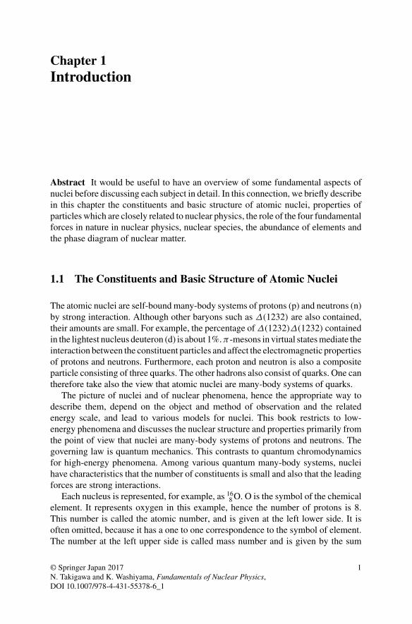
Fig. 1.1 Conceptualillustration of nuclearstructure: example of 4521Sc
of the atomic number and the neutron number. They are denoted by A, Z and N ,respectively, and A = Z + N .
Figure1.1 is a conceptual illustration of nuclear structure exemplified by 4521Sc.
The enclosing circle has been drawn to indicate the finiteness of the nuclear size. Inreality, it is absent, because nuclei are not given by any external boundary conditions,but are self-bound systems. The arrows indicate that protons p and neutrons n inside anucleus are not fixed at lattice points like atoms in solids, but are moving around withfinite velocities. We learn later that nuclei behave like either liquid or gas dependingon the observables or phenomena we are interested in.
1.2 Properties of Particles Relevant to Nuclear Physics
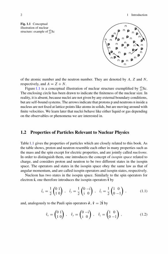
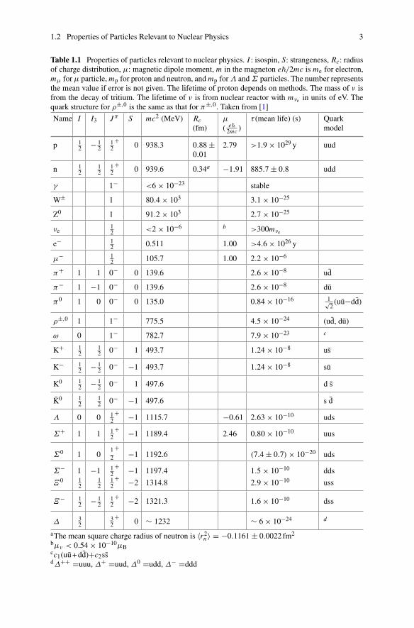
Table1.1 gives the properties of particles which are closely related to this book. Asthe table shows, proton and neutron resemble each other in many properties such asthe mass and the spin except for electric properties, and are jointly called nucleons.In order to distinguish them, one introduces the concept of isospin space related tocharge, and considers proton and neutron to be two different states in the isospinspace. The operators and states in the isospin space obey the same law as that ofangular momentum, and are called isospin operators and isospin states, respectively.
Nucleon has two states in the isospin space. Similarly to the spin operators forelectron s, one therefore introduces the isospin operators t by
tx = 1
2
(0 11 0
), ty = 1
2
(0 −ii 0
), tz = 1
2
(1 00 −1
), (1.1)
and, analogously to the Pauli spin operators σ , τ = 2t by
τx =(0 11 0
), τy =
(0 −ii 0
), τz =
(1 00 −1
), (1.2)
1.2 Properties of Particles Relevant to Nuclear Physics 3
Table 1.1 Properties of particles relevant to nuclear physics. I : isospin, S: strangeness, Rc: radiusof charge distribution, μ: magnetic dipole moment, m in the magneton e�/2mc is me for electron,mμ for μ particle,mp for proton and neutron, andmp forΛ andΣ particles. The number representsthe mean value if error is not given. The lifetime of proton depends on methods. The mass of ν isfrom the decay of tritium. The lifetime of ν is from nuclear reactor with mνe in units of eV. Thequark structure for ρ±,0 is the same as that for π±,0. Taken from [1]
Name I I3 Jπ S mc2 (MeV) Rc(fm)
μ
( e�2mc )
τ (mean life) (s) Quarkmodel
p 12 − 1
212
+0 938.3 0.88 ±
0.012.79 >1.9 × 1029 y uud
n 12
12
12
+0 939.6 0.34a −1.91 885.7 ± 0.8 udd
γ 1− <6 × 10⁻²³ stable
W± 1 80.4 × 10³ 3.1 × 10⁻²⁵
Z0 1 91.2 × 10³ 2.7 × 10⁻²⁵
νe12 <2 × 10⁻⁶ b >300mνe
e− 12 0.511 1.00 >4.6 × 1026 y
μ− 12 105.7 1.00 2.2 × 10⁻⁶
π+ 1 1 0− 0 139.6 2.6 × 10⁻⁸ ud
π− 1 −1 0− 0 139.6 2.6 × 10⁻⁸ du
π0 1 0 0− 0 135.0 0.84 × 10⁻¹⁶ 1√2(uu−dd)
ρ±,0 1 1− 775.5 4.5 × 10⁻²⁴ (ud, du)
ω 0 1− 782.7 7.9 × 10⁻²³ c
K+ 12
12 0− 1 493.7 1.24 × 10⁻⁸ us
K− 12 − 1
2 0− −1 493.7 1.24 × 10⁻⁸ su
K0 12 − 1
2 0− 1 497.6 d s
K0 12
12 0− −1 497.6 s d
Λ 0 0 12
+ −1 1115.7 −0.61 2.63 × 10⁻¹⁰ uds
Σ+ 1 1 12
+ −1 1189.4 2.46 0.80 × 10⁻¹⁰ uus
Σ0 1 012
+ −1 1192.6 (7.4 ± 0.7) × 10−20 uds
Σ− 1 −1 12
+ −1 1197.4 1.5 × 10⁻¹⁰ dds
Ξ0 12
12
12
+ −2 1314.8 2.9 × 10⁻¹⁰ uss
Ξ− 12 − 1
212
+ −2 1321.3 1.6 × 10⁻¹⁰ dss
Δ 32
32
+0 ∼ 1232 ∼ 6 × 10⁻²⁴ d
aThe mean square charge radius of neutron is 〈r2n 〉 = −0.1161 ± 0.0022 fm2
bμν < 0.54 × 10⁻¹⁰μBcc1(uu+dd)+c2ssdΔ++ =uuu, Δ+ =uud, Δ0 =udd, Δ− =ddd
4 1 Introduction
and considers proton and neutron to be simultaneous eigenstates of t2and tz in such
a way that1
|n〉 =∣∣∣∣12
1
2
⟩=
(10
), |p〉 =
∣∣∣∣12 − 1
2
⟩=
(01
). (1.3)
AsTable1.1 shows, the isospin is one of the important quantumnumbers to specifythe property of each particle. Itsmagnitude is assigned to be I when there exist 2I + 1particles which have common properties for all aspects such as the mass and spinbut the electric charge. For example, the isospin of π -mesons is 1, since there existthree particles which differ only in the electric charge. In nuclei, the isospin quantumnumber of each state and the symmetry concerning the isospin play important rolesreflecting the symmetry properties of nuclear force in the isospin space.
If a particle is a structureless fermion, one can deduce from the Dirac equationthat its magnetic dipole moment, which is often simply called magnetic moment,is given by μ = e�/2mc, where m is the mass of the particle. In fact, the magneticmoment of an electron is 1 in units of the Bohr magneton μB = e�/2mec.2 However,Table1.1 shows that the magnetic moment of a proton significantly deviates from thenuclear magneton μN = e�/2mpc. Also, the magnetic moment of a neutron is notzero, but is nearly comparable in magnitude and opposite in sign to that of a proton.They are called anomalous magnetic moments and imply that both the proton andthe neutron are composite particles with intrinsic structure.3
Exercise 1.1 Derive the approximate equation for two large components ϕ in thefour-component spinor ψ starting from the Dirac equation in the presence of elec-tromagnetic fields and assuming that the velocity v of the particle is much smallerthan the speed of light in vacuum c, i.e., v � c, and show that the term whichdescribes the interaction with the magnetic field in the effective Hamiltonian is givenby H = − e�
2mcσ · B, where B is the magnetic field. One can thus prove that themagnetic moment of a Dirac particle is given by e�/2mc.
The fact that both proton and neutron are not point particles, but have intrinsicstructure, can be seen also directly from the data of charge distribution. The radiusof the charge distribution of a proton is about 1 fm.4
1There exists an alternative definition, where proton and neutron are inverted such that |p〉 = | 12 12 〉,
|n〉 = | 12 − 12 〉. Since N ≥ Z for most stable nuclei, we adopt the Definition (1.3) in this book.
2Precisely speaking, the experimental value of the magnetic moment of an electron is larger than theprediction of the Dirac theory by about 0.1%, and can be explained by quantum electrodynamics.3It is Otto Stern who experimentally determined the magnetic moment of a proton for the firsttime. There remains an episode that Pauli visited Stern while he was conducting the experimentand denied the significance of the experiment based on the Dirac theory. Despite the criticism,Stern continued his experiment, and discovered the anomalous magnetic moment of a proton, andconsequently was awarded the Nobel Prize in Physics in 1943.4Recent experiments of the scattering of high-energy electrons, and also of polarized electrons, areshedding new lights on the intrinsic structure of nucleons. For example, it is getting uncovered thatthe electric and magnetic charge distributions are different.
1.2 Properties of Particles Relevant to Nuclear Physics 5
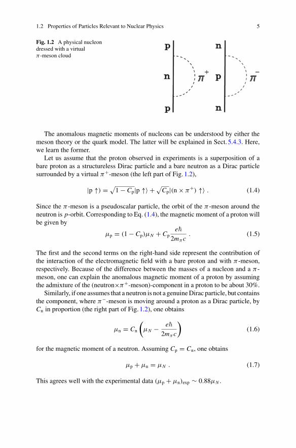
Fig. 1.2 A physical nucleondressed with a virtualπ -meson cloud
The anomalous magnetic moments of nucleons can be understood by either themeson theory or the quark model. The latter will be explained in Sect. 5.4.3. Here,we learn the former.
Let us assume that the proton observed in experiments is a superposition of abare proton as a structureless Dirac particle and a bare neutron as a Dirac particlesurrounded by a virtual π+-meson (the left part of Fig. 1.2),
|p ↑) = √1 − Cp|p ↑〉 + √
Cp|(n × π+) ↑〉 . (1.4)
Since the π -meson is a pseudoscalar particle, the orbit of the π -meson around theneutron is p-orbit. Corresponding to Eq. (1.4), the magnetic moment of a proton willbe given by
μp = (1 − Cp)μN + Cpe�
2mπc. (1.5)
The first and the second terms on the right-hand side represent the contribution ofthe interaction of the electromagnetic field with a bare proton and with π -meson,respectively. Because of the difference between the masses of a nucleon and a π -meson, one can explain the anomalous magnetic moment of a proton by assumingthe admixture of the (neutron×π+-meson)-component in a proton to be about 30%.
Similarly, if one assumes that a neutron is not a genuineDirac particle, but containsthe component, where π−-meson is moving around a proton as a Dirac particle, byCn in proportion (the right part of Fig. 1.2), one obtains
μn = Cn
(μN − e�
2mπc
)(1.6)
for the magnetic moment of a neutron. Assuming Cp = Cn, one obtains
μp + μn = μN . (1.7)
This agrees well with the experimental data (μp + μn)exp ∼ 0.88μN .
6 1 Introduction
1.3 The Role of Various Forces
It is known that four types of forces exist in nature. In this section, we briefly surveythe role of four forces in nuclear physics.
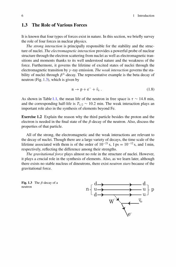
The strong interaction is principally responsible for the stability and the struc-ture of nuclei. The electromagnetic interaction provides a powerful probe of nuclearstructure through the electron scattering from nuclei as well as electromagnetic tran-sitions and moments thanks to its well understood nature and the weakness of theforce. Furthermore, it governs the lifetime of excited states of nuclei through theelectromagnetic transition by γ -ray emission. The weak interaction governs the sta-bility of nuclei through β±-decay. The representative example is the beta decay ofneutron (Fig. 1.3), which is given by
n → p + e− + νe . (1.8)
As shown in Table1.1, the mean life of the neutron in free space is τ ∼ 14.8 min,and the corresponding half-life is T1/2 ∼ 10.2 min. The weak interaction plays animportant role also in the synthesis of elements beyond Fe.
Exercise 1.2 Explain the reason why the third particle besides the proton and theelectron is needed in the final state of the β-decay of the neutron. Also, discuss theproperties of that particle.
All of the strong, the electromagnetic and the weak interactions are relevant tothe decay of nuclei. Though there are a large variety of decays, the time scale of thelifetime associated with them is of the order of 10−21 s, 1 ps = 10−12 s, and 1min,respectively, reflecting the difference among their strengths.
The gravitational force plays almost no role in the structure of nuclei. However,it plays a crucial role in the synthesis of elements. Also, as we learn later, althoughthere exists no stable nucleus of dineutrons, there exist neutron stars because of thegravitational force.
Fig. 1.3 The β-decay of aneutron
1.4 Useful Physical Quantities 7
1.4 Useful Physical Quantities
It is sometimesworthmaking order-of-magnitude estimates of various physical quan-tities. In that connection. it is useful to remember the following approximate valuesrelated to the fundamental physical constants c (the speed of light in vacuum), � (thePlanck constant divided by 2π ), e (electron charge magnitude), kB (the Boltzmannconstant) as
c = 2.99792458 × 10⁸ m/s ≈ 3.00 × 10⁸ m/s, (1.9)
�c = 197.326968MeV fm ≈ 200MeV fm, (1.10)
e2
�c= 1
137.035999074≈ 1
137(fine structure constant), (1.11)
kBT = 0.02482 eV ≈ 1
40eV at T = 288K. (1.12)
The quantity e2/�c is called the fine structure constant. Equation (1.11) holds whenthe proportional coefficient in the static electric force between two particles withelectric charge q1, q2 is determined such that the force is given by F(r) = q1q2/r2
when the two particles are apart from each other by the distance r . Equation (1.12)represents the kinetic energy of thermal neutrons. It is useful to convert the temper-ature given in units of Kelvin to the corresponding energy in units of MeV.
Exercise 1.3 The range of force is given by the Compton wave length �/mc of thecorresponding gauge particle. Estimate the range of the strong interaction and of theweak interaction.
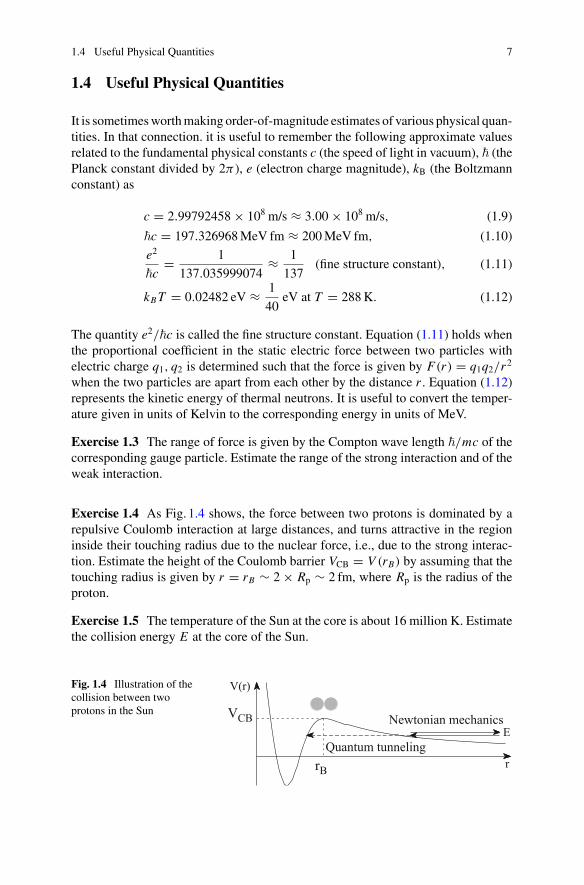
Exercise 1.4 As Fig. 1.4 shows, the force between two protons is dominated by arepulsive Coulomb interaction at large distances, and turns attractive in the regioninside their touching radius due to the nuclear force, i.e., due to the strong interac-tion. Estimate the height of the Coulomb barrier VCB = V (rB) by assuming that thetouching radius is given by r = rB ∼ 2 × Rp ∼ 2 fm, where Rp is the radius of theproton.
Exercise 1.5 The temperature of the Sun at the core is about 16 million K. Estimatethe collision energy E at the core of the Sun.
Fig. 1.4 Illustration of thecollision between twoprotons in the Sun
ENewtonian mechanics
Quantum tunnelingrrB
V(r)
VCB
8 1 Introduction
Nuclear reactions in the Sun occur very slowly, because they take place by quan-tum tunneling as indicated by Exercises1.4 and 1.5. In reality, there exists anotherimportant hindrance factor. As we learn later, there exists no stable bound state in thediproton system. The only stable dinucleon system is deuteron consisting of one pro-ton and one neutron. In order for the fusion of two protons to take place, the inversereaction of Eq. (1.8), where a proton is converted into a neutron by weak interaction,must therefore be involved. Because of the superposition of the quantum tunnelingand weak interaction, the nuclear reaction between two protons is doubly hindered.Consequently, the Sun burns very slowly. It has burnt already for 4.6 billion yearsand is expected to continue to shine for another almost same period.
1.5 Species of Nuclei
The display of nuclei on the two-dimensional plane, where one axis, say the abscissa,represents the neutron number and the other, say the ordinate, the proton number, iscalledNuclear chart or Segré chart. There are 256 stable nuclei if one includes thosenuclei which have long lifetimes of the order comparable to the lifetime of the Sunsuch as U. They lie in the vicinity of the diagonal line of the nuclear chart for thereason we learn later. The reason why there exist more stable nuclei than the numberof stable elements about 92 in nature is because there exist about three stable nucleifor each element on average. For example, there exist two stable nuclei, called protonp and deuteron d, for the element hydrogen.
Incidentally, the nuclei which have the same number of protons (i.e., the sameatomic number), but differ in the neutron number, hence in the mass number as well,are called isotopes to each other, and those whose neutron numbers are the same,but the proton numbers are different, the isotones, and those which have same massnumbers the isobars, respectively.
The study of unstable nucleiwith short lifetimes is currently one of the hot subjectsof nuclear physics. If one includes unstable nuclei whose lifetime is longer than 1µs,about 7000 nuclei are theoretically predicted to exist, amongwhich about 3000 nucleihave already been discovered experimentally. Also, a group of nuclei stabilized byshell effects (see Chap.5) are predicted to exist in the region far beyond U. Theyare called superheavy nuclei or superheavy elements, on which extensive studies aregoing on both experimentally and theoretically.
1.5 Species of Nuclei 9
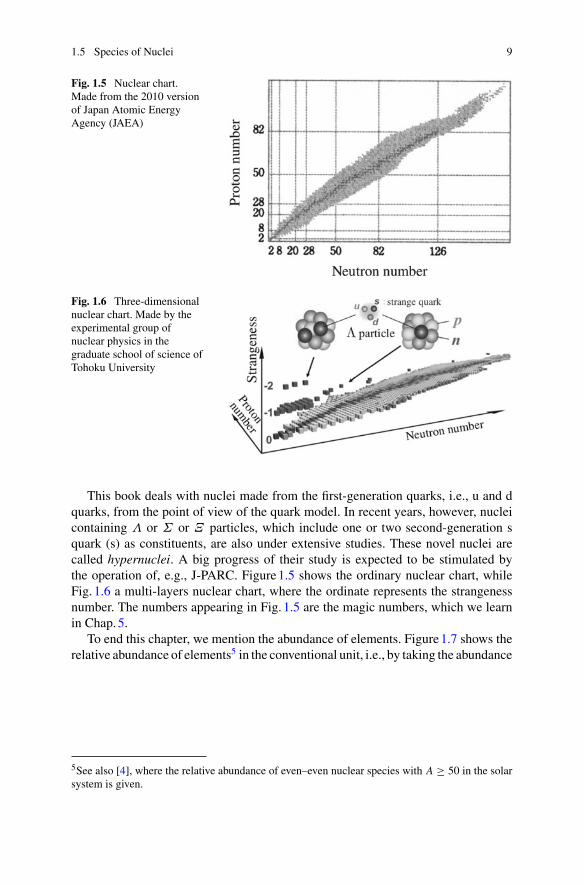
Fig. 1.5 Nuclear chart.Made from the 2010 versionof Japan Atomic EnergyAgency (JAEA)
Fig. 1.6 Three-dimensionalnuclear chart. Made by theexperimental group ofnuclear physics in thegraduate school of science ofTohoku University
This book deals with nuclei made from the first-generation quarks, i.e., u and dquarks, from the point of view of the quark model. In recent years, however, nucleicontaining Λ or Σ or Ξ particles, which include one or two second-generation squark (s) as constituents, are also under extensive studies. These novel nuclei arecalled hypernuclei. A big progress of their study is expected to be stimulated bythe operation of, e.g., J-PARC. Figure1.5 shows the ordinary nuclear chart, whileFig. 1.6 a multi-layers nuclear chart, where the ordinate represents the strangenessnumber. The numbers appearing in Fig. 1.5 are the magic numbers, which we learnin Chap.5.
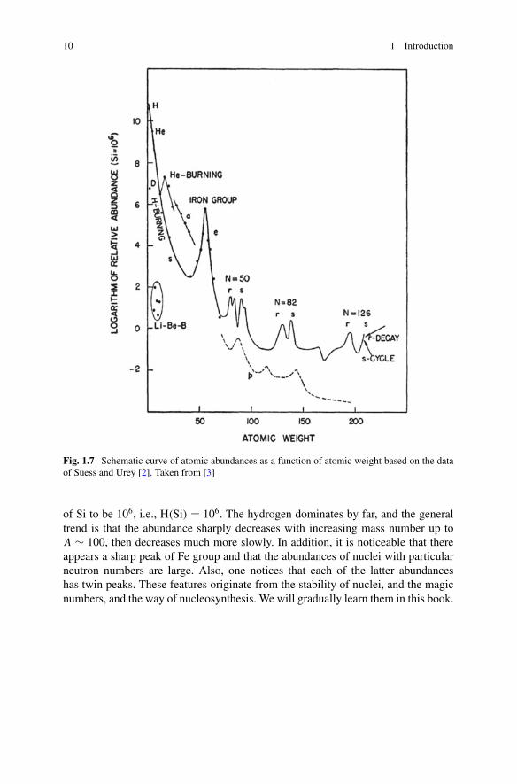
To end this chapter, we mention the abundance of elements. Figure1.7 shows therelative abundance of elements5 in the conventional unit, i.e., by taking the abundance
5See also [4], where the relative abundance of even–even nuclear species with A ≥ 50 in the solarsystem is given.
10 1 Introduction
Fig. 1.7 Schematic curve of atomic abundances as a function of atomic weight based on the dataof Suess and Urey [2]. Taken from [3]
of Si to be 106, i.e., H(Si) = 106. The hydrogen dominates by far, and the generaltrend is that the abundance sharply decreases with increasing mass number up toA ∼ 100, then decreases much more slowly. In addition, it is noticeable that thereappears a sharp peak of Fe group and that the abundances of nuclei with particularneutron numbers are large. Also, one notices that each of the latter abundanceshas twin peaks. These features originate from the stability of nuclei, and the magicnumbers, and the way of nucleosynthesis. We will gradually learn them in this book.
1.6 Column: QCD Phase Diagram of Nuclear Matter 11
1.6 Column: QCD Phase Diagram of Nuclear Matter
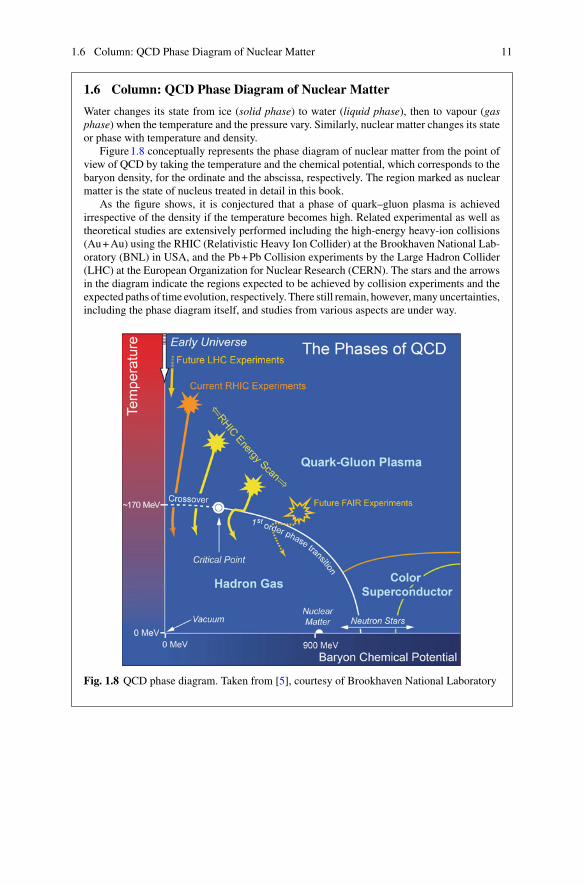
Water changes its state from ice (solid phase) to water (liquid phase), then to vapour (gasphase) when the temperature and the pressure vary. Similarly, nuclear matter changes its stateor phase with temperature and density.
Figure1.8 conceptually represents the phase diagram of nuclear matter from the point ofview of QCD by taking the temperature and the chemical potential, which corresponds to thebaryon density, for the ordinate and the abscissa, respectively. The region marked as nuclearmatter is the state of nucleus treated in detail in this book.
As the figure shows, it is conjectured that a phase of quark–gluon plasma is achievedirrespective of the density if the temperature becomes high. Related experimental as well astheoretical studies are extensively performed including the high-energy heavy-ion collisions(Au+Au) using the RHIC (Relativistic Heavy Ion Collider) at the Brookhaven National Lab-oratory (BNL) in USA, and the Pb+Pb Collision experiments by the Large Hadron Collider(LHC) at the European Organization for Nuclear Research (CERN). The stars and the arrowsin the diagram indicate the regions expected to be achieved by collision experiments and theexpected paths of time evolution, respectively. There still remain, however,many uncertainties,including the phase diagram itself, and studies from various aspects are under way.
Fig. 1.8 QCD phase diagram. Taken from [5], courtesy of Brookhaven National Laboratory

12 1 Introduction
References
1. W.-M. Yao et al. (Particle Data Group), J. Phys. G 33, 1 (2006)2. H.E. Suess, H.C. Urey, Rev. Mod. Phys. 28, 53 (1956)3. E.M. Burbidge, G.R. Burbidge, W.A. Fowler, F. Hoyle, Rev. Mod. Phys. 29, 547 (1957)4. Aage Bohr, Ben R. Mottelson, Nuclear Structure, vol. I (Benjamin, New York, 1969)5. The Nuclear Science Advisory Committee, The Frontiers of Nuclear Science – A Long Range
Plan (2007). http://science.energy.gov/np/nsac/
Chapter 2Bulk Properties of Nuclei
Abstract Their sizes andmasses are themost fundamental properties of nuclei. Theyhave simple mass number dependences which suggest that the nucleus behaves like aliquid and lead to the liquid-dropmodel for the nucleus. In this chapter we learn thesebulk properties of nuclei and their applications to discussing nuclear stability, muon-catalysed fusion and the structure of heavy stars. As an example of the applicationswe discuss somewhat in detail the basic features of fission and nuclear reactors. Wealso mention deviations from what are expected from the liquid-drop model whichsuggest the pairing correlation and shell effects. We also discuss the velocity and thedensity distributions of nucleons inside a nucleus.
2.1 Nuclear Sizes
2.1.1 Rutherford Scattering
At the beginning of the twentieth centurywhen quantummechanicswas born, variousmodels were proposed for the structure of atoms such as the plum pudding or raisinbread model of J.J. Thompson, which assumes that the plus charge distributes overwhole atom together with electrons, and the Saturn model by Hantaro Nagaoka.Rutherford led these debates to conclusion through the study of scattering of alphaparticles on atom. He proposed the existence of a central part of the atom, i.e., thecore part, which bears all the positive charge that cancels out the total negative chargeof electrons and also carries the dominant part of the mass of the atom. Rutherfordnamed this core part nucleus, and gave the limiting value to its size.1 At that time,Rutherford hadbeen engaged in the detailed studies of the properties of alphaparticlesemitted from radioactive materials, and knew that the alpha particle is the ionizedHe. What Rutherford remarked in the experimental results of Marsden is that alpha
1It was 1911 when Rutherford submitted his article on the atomic model to a science journal.The idea and the formula of Rutherford were derived by stimulation of experimental results of hiscoworker Marsden who had been engaged in the study of scattering of alpha particles emitted fromnatural radioactive elements on matter. Furthermore, they have been confirmed experimentally tobe correct by his collaborators Geiger and Marsden.
© Springer Japan 2017N. Takigawa and K. Washiyama, Fundamentals of Nuclear Physics,DOI 10.1007/978-4-431-55378-6_2
13
14 2 Bulk Properties of Nuclei
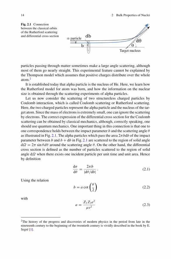
Fig. 2.1 Connectionbetween the classical orbitsof the Rutherford scatteringand differential cross section
particles passing through matter sometimes make a large angle scattering, althoughmost of them go nearly straight. This experimental feature cannot be explained bythe Thompson model which assumes that positive charges distribute over the wholeatom.2
It is established today that alpha particle is the nucleus of He. Here, we learn howthe Rutherford model for atom was born, and how the information on the nuclearsize is obtained through the scattering experiments of alpha particles.
Let us now consider the scattering of two structureless charged particles byCoulomb interaction, which is called Coulomb scattering or Rutherford scattering.Here, the two charged particles represent the alpha particle and the nucleus of the tar-get atom. Since themass of electrons is extremely small, one can ignore the scatteringby electrons. The correct expression of the differential cross section for the Coulombscattering can be obtained by classical mechanics, although, correctly speaking, oneshould use quantum mechanics. One important thing in this connection is that one toone correspondence holds between the impact parameter b and the scattering angle θ
as illustrated in Fig. 2.1. The alpha particles which pass the area 2πbdb of the impactparameter between b and b + db in Fig. 2.1 are scattered to the region of solid angledΩ = 2π sin θdθ around the scattering angle θ . On the other hand, the differentialcross section is defined as the number of particles scattered to the region of solidangle dΩ when there exists one incident particle per unit time and unit area. Henceby definition
dσ
dθ= 2πb
|dθ/db| . (2.1)
Using the relation
b = a cot
(θ
2
)(2.2)
with
a = Z1Z2e2
μv2(2.3)
2The history of the progress and discoveries of modern physics in the period from late in thenineteenth century to the beginning of the twentieth century is vividly described in the book by E.Segré [1].
2.1 Nuclear Sizes 15
which holds between the impact parameter b and the scattering angle θ in the caseof Coulomb scattering, we obtain
dσ
dΩ= dσR
dΩ≡ 1
2π sin θ
dσ
dθ= a2
4
1
sin4(θ/2), (2.4)
where the indexR inσR means theRutherford scattering. In Eq. (2.3),μ is the reducedmass, and v is the speed of the relative motion in the asymptotic region, i.e., at thebeginning of scattering. Note that Eq. (2.4) exactly agrees with the formula of thedifferential cross section dσR/dΩ obtained quantummechanically for theRutherfordscattering. The characteristics of the Coulomb scattering given by Eq. (2.4) are thatthe forward scattering is strong, but also that backward scattering takes place with acertain probability as well. These match the experimental results of Marsden.
The ground state of the natural radioactive nucleus 21084 Po decays with the half-life
of 138.4 days by emitting an alpha particle (21084 Po → 20682 Pb + α). The kinetic energy
of the alpha particle is about 5.3MeV corresponding to the Q-value of the decay5.4MeV. The differential cross section for the scattering, where this α particle is usedto bombard the Au target of atomic number 79, agrees with that for the Rutherfordscattering right up to the backward angle θ = π . This suggests that the sum of theradii of Au and α (R(Au) + R(α)) is smaller than the distance of closest approachd(θ = π) for the scattering with the impact parameter b = 0 leading to the backwardscattering θ = 180◦ in the case of Rutherford scattering. Since the distance of closestapproach d and the scattering angle θ or the impact parameter b is related by
d = a
[1 + csc
(θ
2
)]= a +
√a2 + b2 (2.5)
for theRutherford scattering, the abovementioned experimental results give the upperboundary of the radius as R(Au) + R(α) < 4.3 × 10⁻¹² cm. This upper boundary ismuch smaller than the radii of atoms, which are of the order of 10−8 cm. Rutherfordwas thus guided to his atomic model.
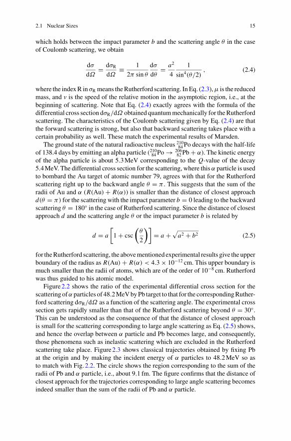
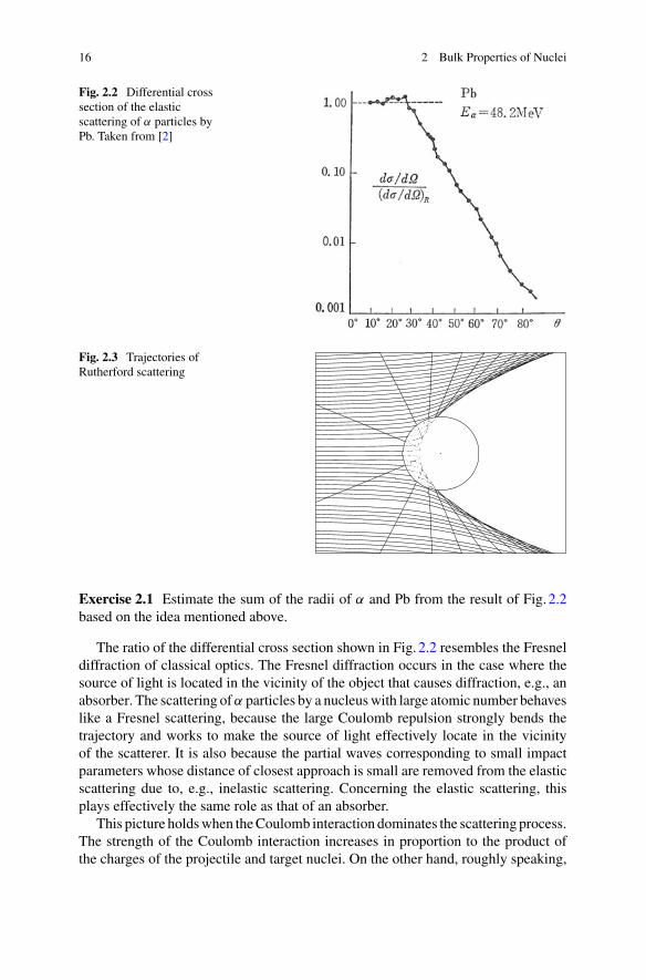
Figure2.2 shows the ratio of the experimental differential cross section for thescattering ofα particles of 48.2MeVbyPb target to that for the correspondingRuther-ford scattering dσR/dΩ as a function of the scattering angle. The experimental crosssection gets rapidly smaller than that of the Rutherford scattering beyond θ = 30◦.This can be understood as the consequence of that the distance of closest approachis small for the scattering corresponding to large angle scattering as Eq. (2.5) shows,and hence the overlap between α particle and Pb becomes large, and consequently,those phenomena such as inelastic scattering which are excluded in the Rutherfordscattering take place. Figure2.3 shows classical trajectories obtained by fixing Pbat the origin and by making the incident energy of α particles to 48.2MeV so asto match with Fig. 2.2. The circle shows the region corresponding to the sum of theradii of Pb and α particle, i.e., about 9.1 fm. The figure confirms that the distance ofclosest approach for the trajectories corresponding to large angle scattering becomesindeed smaller than the sum of the radii of Pb and α particle.
16 2 Bulk Properties of Nuclei
Fig. 2.2 Differential crosssection of the elasticscattering of α particles byPb. Taken from [2]
Fig. 2.3 Trajectories ofRutherford scattering
Exercise 2.1 Estimate the sum of the radii of α and Pb from the result of Fig. 2.2based on the idea mentioned above.
The ratio of the differential cross section shown in Fig. 2.2 resembles the Fresneldiffraction of classical optics. The Fresnel diffraction occurs in the case where thesource of light is located in the vicinity of the object that causes diffraction, e.g., anabsorber. The scattering ofα particles by a nucleuswith large atomic number behaveslike a Fresnel scattering, because the large Coulomb repulsion strongly bends thetrajectory and works to make the source of light effectively locate in the vicinityof the scatterer. It is also because the partial waves corresponding to small impactparameters whose distance of closest approach is small are removed from the elasticscattering due to, e.g., inelastic scattering. Concerning the elastic scattering, thisplays effectively the same role as that of an absorber.
This picture holdswhen theCoulomb interaction dominates the scattering process.The strength of the Coulomb interaction increases in proportion to the product ofthe charges of the projectile and target nuclei. On the other hand, roughly speaking,
2.1 Nuclear Sizes 17
the strength of the nuclear interaction increases in proportion to the reduced massA1A2/(A1 + A2). Hence the refraction effect due to the nuclear interaction becomesnon-negligible for the scattering by a target nucleus with small atomic number. Infact, a similar differential cross section appears not by diffraction effect, but byrefraction effect. The interpretation and analysis then get complicated. Accordingly,one can safely estimate the nuclear size based on the consideration of the Coulombtrajectory together with the strong absorption due to inelastic scattering as describedin the present section when the atomic number of the target nucleus is large.
2.1.2 Electron Scattering
The scattering of α particles by a nucleus had led to the Rutherford atomic model,and provided a way to estimate the nuclear size. It thus played an important historicalrole. However, as stated at the end of the last section, it has a limitation regardingapplicability. In contrast, the scattering of electrons by a nucleus, which we learn inthis section, is a powerful method to study the nuclear size, more exactly, the dis-tribution of protons inside a nucleus, because only well understood electromagneticforce is involved.3,4
2.1.2.1 The de Broglie Wavelength of Electron
In the experiments of electron scattering, electrons are injected on the target nucleusafter they are accelerated by, e.g., a linear accelerator. In order to deduce the infor-mation on the nuclear size from electron scattering, the de Broglie wavelength of theelectron must be of the same order of magnitude as that of the nuclear size or smaller.In this connection, let us first study the relation between the de Broglie wavelengthof electron and the kinetic energy of electron supplied by the accelerator.
The de Broglie wavelength of electron λe is given by
λe = h
pe(2.6)
in terms of the momentum of the electron pe and the Planck constant h. On the otherhand, it holds that
Etotal =√
m2ec4 + p2
ec2 = mec2 + Ekin = mec
2 + Ee (2.7)
3R. Hofstadter was awarded the Nobel Prize in Physics 1961 for the study of high energy electronscattering with linear accelerator and the discovery of the structure of nucleon. He performed alsosystematic studies of nuclei by electron scattering.4The electron scattering is a powerful method to learn the structure of nucleons mentioned inChap.1, and also to study nuclear excitations such as giant resonances and hypernuclei as well.
18 2 Bulk Properties of Nuclei
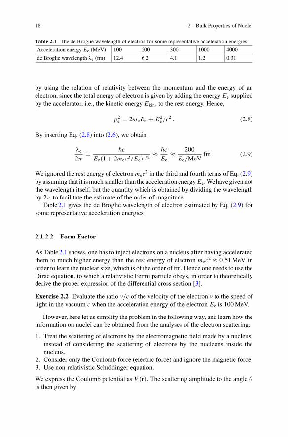
Table 2.1 The de Broglie wavelength of electron for some representative acceleration energies
Acceleration energy Ee (MeV) 100 200 300 1000 4000
de Broglie wavelength λe (fm) 12.4 6.2 4.1 1.2 0.31
by using the relation of relativity between the momentum and the energy of anelectron, since the total energy of electron is given by adding the energy Ee suppliedby the accelerator, i.e., the kinetic energy Ekin, to the rest energy. Hence,
p2e = 2meEe + E2
e /c2 . (2.8)
By inserting Eq. (2.8) into (2.6), we obtain
λe
2π= �c
Ee(1 + 2mec2/Ee)1/2≈ �c
Ee≈ 200
Ee/MeVfm . (2.9)
We ignored the rest energy of electron mec2 in the third and fourth terms of Eq. (2.9)by assuming that it ismuch smaller than the acceleration energy Ee.Wehavegivennotthe wavelength itself, but the quantity which is obtained by dividing the wavelengthby 2π to facilitate the estimate of the order of magnitude.
Table2.1 gives the de Broglie wavelength of electron estimated by Eq. (2.9) forsome representative acceleration energies.
2.1.2.2 Form Factor
As Table2.1 shows, one has to inject electrons on a nucleus after having acceleratedthem to much higher energy than the rest energy of electron mec2 ≈ 0.51MeV inorder to learn the nuclear size, which is of the order of fm. Hence one needs to use theDirac equation, to which a relativistic Fermi particle obeys, in order to theoreticallyderive the proper expression of the differential cross section [3].
Exercise 2.2 Evaluate the ratio v/c of the velocity of the electron v to the speed oflight in the vacuum c when the acceleration energy of the electron Ee is 100MeV.
However, here let us simplify the problem in the following way, and learn how theinformation on nuclei can be obtained from the analyses of the electron scattering:
1. Treat the scattering of electrons by the electromagnetic field made by a nucleus,instead of considering the scattering of electrons by the nucleons inside thenucleus.
2. Consider only the Coulomb force (electric force) and ignore the magnetic force.3. Use non-relativistic Schrödinger equation.
We express the Coulomb potential as V (r). The scattering amplitude to the angle θ
is then given by
2.1 Nuclear Sizes 19
f (1)(θ) = − 1
4π
2μ
�2
∫e−iq·rV (r)dr (2.10)
following the first order Born approximation, which is valid because of the highenergy scattering, and also because the involved electric force is weak compared tothe kinetic energy. The μ is the reduced mass. It can be identified with the mass ofelectron me to a high degree of accuracy. The q is the momentum transfer dividedby � and is given by
q = kf − ki , (2.11)
q = |q| = 2k sin(θ/2) . (2.12)
where ki is the wave-vector of the incident electron, kf is the wave-vector of theelectron scattered to the direction of angle θ and k is the wave number of the electroncorresponding to the incident energy.
Exercise 2.3 Derive Eqs. (2.10)–(2.12).
We remark that the potential V (r) obeys the following Poisson equation,
ΔV = 4π Ze2ρC(r) , (2.13)
in order to relate the scattering amplitude to the distribution of protons inside anucleus. The Z is the atomic number of the nucleus to be studied, and ρC(r) isthe charge density at the position r measured from the center of the nucleus.5 It isnormalized as ∫
ρC(r)dr = 1 . (2.14)
By repeating the integration by parts twice in Eq. (2.10), and by using Eq. (2.13), weobtain,
f (1)(θ) = Ze2
2μv21
sin2(θ/2)F(q) , (2.15)
where F(q) is defined as
F(q) ≡∫
e−iq·rρC(r)dr . (2.16)
The differential cross section is therefore given by
dσ (1)
dΩ= | f (1)(θ)|2 = dσR
dΩ|F(q)|2 . (2.17)
5The distribution of protons ρp can be derived from ρC by taking into account the intrinsic structureof proton.
20 2 Bulk Properties of Nuclei
Correctly, the expression of the differential cross section is obtained as
dσ (1)
dΩ= dσM
dΩ|F(q)|2 , (2.18)
dσM
dΩ=
[Ze2
2Ee sin2(θ/2)
]2 [1 − v2
c2sin2(θ/2)
]
≈[
Ze2 cos(θ/2)
2Ee sin2(θ/2)
]2
, (2.19)
by replacing the differential cross section of the Rutherford scattering dσR/dΩ bythat for the Mott scattering dσM/dΩ which takes into account relativistic effectsfor electrons. The dσM/dΩ gives the differential cross section of the scattering ofelectrons by the Coulomb force made by a point charge. Equation (2.18) shows thatthe information on the density distribution of protons inside a nucleus can be obtainedthrough the ratio of the experimental differential cross section to that for the Mottscattering. The F(q) defined by Eq. (2.16) is the factor which represents the effectsof the finiteness of the nuclear size and is called the form factor.
Especially, if the nucleus is spherical, i.e., if the charge distribution is spherical,the form factor is given by
F(q) = 4π∫ ∞
0ρC(r) j0(qr)r2dr = 4π
∫ ∞
0ρC(r)
sin(qr)
qrr2dr , (2.20)
where j0(x) is the spherical Bessel function of the first kind.
Exercise 2.4 Prove Eq. (2.20) in the following two methods:
1. Perform directly the integration over the angular part of r (dΩr ) in Eq. (2.16).2. Expand at first the e−iq·r in terms of Legendre functions, and then use the ortho-
normal property of the spherical harmonics.
2.1.2.3 Density Distribution
(1) Estimate of theNuclearRadius fromDiffraction PatternAsTable2.1 implies,the experiments of electron scattering are performed with high energy in order tostudy nuclear size and the density distribution of protons inside a nucleus. The cor-responding differential cross section is expected to show a diffraction pattern similarto that of the Fraunhofer diffraction in optics. Figure2.4 shows the differential crosssection for the elastic scattering of electrons fromAu target at 153 and 183MeV. Themonotonically decreasing solid line is the Mott scattering cross section for 183MeV.The figure shows that the observed cross section is smaller than that for theMott scat-tering, and that it has indeed the diffraction pattern, i.e., oscillation, of the Fraunhofertype.
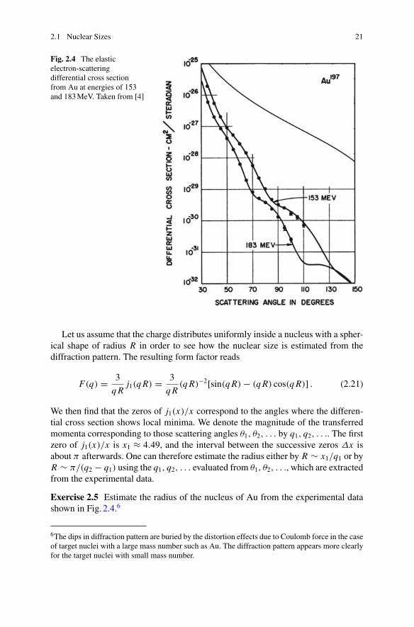
2.1 Nuclear Sizes 21
Fig. 2.4 The elasticelectron-scatteringdifferential cross sectionfrom Au at energies of 153and 183MeV. Taken from [4]
Let us assume that the charge distributes uniformly inside a nucleus with a spher-ical shape of radius R in order to see how the nuclear size is estimated from thediffraction pattern. The resulting form factor reads
F(q) = 3
q Rj1(q R) = 3
q R(q R)−2[sin(q R) − (q R) cos(q R)] . (2.21)
We then find that the zeros of j1(x)/x correspond to the angles where the differen-tial cross section shows local minima. We denote the magnitude of the transferredmomenta corresponding to those scattering angles θ1, θ2, . . . by q1, q2, . . .. The firstzero of j1(x)/x is x1 ≈ 4.49, and the interval between the successive zeros Δx isabout π afterwards. One can therefore estimate the radius either by R ∼ x1/q1 or byR ∼ π/(q2 − q1) using the q1, q2, . . . evaluated from θ1, θ2, . . ., which are extractedfrom the experimental data.
Exercise 2.5 Estimate the radius of the nucleus of Au from the experimental datashown in Fig. 2.4.6
6The dips in diffraction pattern are buried by the distortion effects due to Coulomb force in the caseof target nuclei with a large mass number such as Au. The diffraction pattern appears more clearlyfor the target nuclei with small mass number.
22 2 Bulk Properties of Nuclei
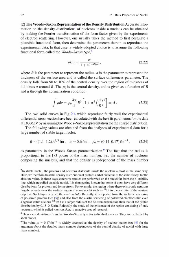
(2) TheWoods–SaxonRepresentation of theDensityDistributionAccurate infor-mation on the density distribution7 of nucleons inside a nucleus can be obtainedby making the Fourier transformation of the form factor given by the experimentsof electron scattering. However, one usually takes the method to first postulate aplausible functional form, then determine the parameters therein to reproduce theexperimental data. In that case, a widely adopted choice is to assume the followingfunctional form called the Woods–Saxon type,8
ρ(r) = ρ0
1 + e(r−R)/a, (2.22)
where R is the parameter to represent the radius. a is the parameter to represent thethickness of the surface area and is called the surface diffuseness parameter. Thedensity falls from 90 to 10% of the central density over the region of thickness of4.4 times a around R. The ρ0 is the central density, and is given as a function of Rand a through the normalization condition,
∫ρdr ∼ ρ0
4π
3R3
[1 + π2
( a
R
)2]
= A . (2.23)
The two solid curves in Fig. 2.4 which reproduce fairly well the experimentaldifferential cross section have been calculated with the best fit parameters for the dataat 183MeVby assuming theWoods–Saxon representation for the charge distribution.
The following values are obtained from the analyses of experimental data for alarge number of stable target nuclei,
R ∼ (1.1–1.2)A1/3 fm , a ∼ 0.6 fm , ρ0 ∼ (0.14–0.17) fm−3 , (2.24)
as parameters in the Woods–Saxon parametrization.9 The fact that the radius isproportional to the 1/3 power of the mass number, i.e., the number of nucleonscomposing the nucleus, and that the density is independent of the mass number
7In stable nuclei, the protons and neutrons distribute inside the nucleus almost in the same way.Here, we therefore treat the density distribution of protons and of nucleons as the same except for theabsolute value. In these days, extensive studies are performed on the nuclei far from the β-stabilityline, which are called unstable nuclei. It is then getting known that some of them have very differentdistributions for protons and for neutrons. For example, the region where there exists only neutronslargely extends over the surface region in some nuclei such as 11Li in the vicinity of the neutrondrip line. Such layer is called the neutron halo. Recently, it is reported from the inelastic scatteringof polarized protons (see [5]) and also from the elastic scattering of polarized electrons that evena typical stable nucleus 208Pb has a larger radius of the neutron distribution than that of the protondistribution by 0.15–0.33 fm. Relatedly, the study of the existence of the region consisting of onlyneutrons, which is called neutron skin, is an active area of research.8There exist deviations from the Woods–Saxon type for individual nucleus. They are explained byshell model.9The value ρ0 ∼ 0.17 fm−3 is widely accepted as the density of nuclear matter (see [6] for theargument about the detailed mass number dependence of the central density of nuclei with largemass number).
2.1 Nuclear Sizes 23
suggest that the nucleus has a property as a liquid.10 The fact that the density isindependent of the mass number is called the saturation property of nuclear density.
Incidentally, the surface area dominates in light nuclei. The Gaussian type istherefore often used, instead of theWoods–Saxon type, as a more realistic functionalform.
2.1.2.4 The Root-Mean-Square Radius
The radius of a nucleus is the average of the radii of the region of spatial occupation ofthe nucleons composing the nucleus. Hence the concept of root-mean-square radiusis often used in discussing nuclear size. We first define the mean-square radius by
⟨r2
⟩ ≡∫ ∞
0r2ρ(r)4πr2dr
/∫ ∞
0ρ(r)4πr2dr . (2.25)
The root-mean-square radius Rr.m.s. is then defined by taking the square root asRr.m.s. ≡ √〈r2〉.
We assumed a sharp density distribution without a surface diffuseness, i.e., a stepfunction, in a simple analysis of the diffraction pattern of the electron scattering,e.g., as shown in Eq. (2.21). We name the resulting radius the equivalent radius orthe effective sharp radius and designate it as Req. By definition, Rr.m.s. and Req arerelated to each other as
Req =√5
3〈r2〉 =
√5
3Rr.m.s. . (2.26)
Since Req is proportional to the 1/3 power of the mass number A, let us represent itas
Req = r0 A1/3 . (2.27)
The proportional coefficient r0, called radius parameter, is then independent ofindividual nucleus, and takes experimentally the value11 of
r0 ∼ 1.1–1.2 fm . (2.28)
10Although the nucleus appears like a drop of liquid, it is not a classical liquid, but a drop of quantumliquid, since commutation relations govern the nucleus. In the classical liquid, the momentum spaceis not deformed even if it is spatially deformed. On the other hand, in the case of nuclei, a spatialdeformation leads to the deformation in the momentum space through the uncertainty relation (seethe footnote concerning quantum liquid in Sect. 8.3.4).11Equations (2.24), (2.27) and (2.28) hold for stable nuclei. It has been found that the radii ofunstable nuclei, especially of nuclei in the vicinity of neutron drip line, significantly deviate fromthese equations. For example, in the case of Li isotopes, the radius of 11Li which has a neutron haloas mentioned before and thus called a halo nucleus or a neutron halo nucleus is much larger thanwhat we expect from Eq. (2.27), although the radii of stable isotopes 6,7Li and of the isotopes 8,9Liwhich lie close to the stability line vary with A almost following Eq. (2.27).
24 2 Bulk Properties of Nuclei
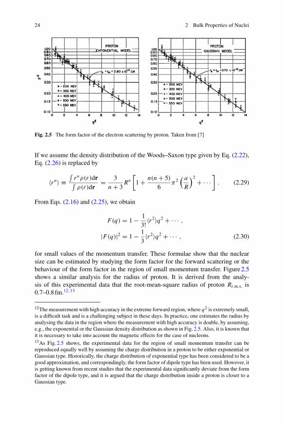
Fig. 2.5 The form factor of the electron scattering by proton. Taken from [7]
If we assume the density distribution of the Woods–Saxon type given by Eq. (2.22),Eq. (2.26) is replaced by
〈rn〉 ≡∫
rnρ(r)dr∫ρ(r)dr
= 3
n + 3Rn
[1 + n(n + 5)
6π2
( a
R
)2 + · · ·]
. (2.29)
From Eqs. (2.16) and (2.25), we obtain
F(q) = 1 − 1
3! 〈r2〉q2 + · · · ,
|F(q)|2 = 1 − 1
3〈r2〉q2 + · · · , (2.30)
for small values of the momentum transfer. These formulae show that the nuclearsize can be estimated by studying the form factor for the forward scattering or thebehaviour of the form factor in the region of small momentum transfer. Figure2.5shows a similar analysis for the radius of proton. It is derived from the analy-sis of this experimental data that the root-mean-square radius of proton Rr.m.s. is0.7–0.8 fm.12,13
12The measurement with high accuracy in the extreme forward region, where q2 is extremely small,is a difficult task and is a challenging subject in these days. In practice, one estimates the radius byanalysing the data in the region where the measurement with high accuracy is doable, by assuming,e.g., the exponential or the Gaussian density distribution as shown in Fig. 2.5. Also, it is known thatit is necessary to take into account the magnetic effects for the case of nucleons.13As Fig. 2.5 shows, the experimental data for the region of small momentum transfer can bereproduced equally well by assuming the charge distribution in a proton to be either exponential orGaussian type. Historically, the charge distribution of exponential type has been considered to be agood approximation, and correspondingly, the form factor of dipole type has been used. However, itis getting known from recent studies that the experimental data significantly deviate from the formfactor of the dipole type, and it is argued that the charge distribution inside a proton is closer to aGaussian type.
2.1 Nuclear Sizes 25
Exercise 2.6 The radius of the charge distribution of a nucleus can be estimatedalso from the energy spectrum of the X-ray of the corresponding muonic-atom, orthe energy difference between the corresponding energy levels of mirror nuclei.14
Study the principle of each method.
2.1.3 Mass Distribution
All the methods mentioned above are the method to study the distribution of protons,in other words, the charge distribution in nuclei, and give no information on thedistributionof neutrons.Onehas to use othermethods in order to study thedistributionof nucleons including neutrons, which is often called the mass distribution, insidea nucleus. The scattering of protons or neutrons by a nucleus, where the stronginteraction is involved, and nucleus-nucleus collisions are the examples. Similarlyto the case of electron scattering, high incident energies are appropriate. Here weconsider two methods.
2.1.3.1 High-Energy Neutron Scattering: Fraunhofer Scattering
Let us first consider the high-energy neutron scattering. Since the interaction betweentheneutron and the target nucleus is strong, neutrons are absorbedor the target nucleusis excited when the neutrons reach the area of the target nucleus. The associated crosssection, i.e., the sum of the cross sections of inelastic scattering and of absorption, isintuitively expected to be given by σ (inel) ∼ π R2 by using the nuclear radius R. Onthe other hand, in the scattering of relatively high energy by a short range interaction,the elastic scattering corresponds to the shadow scattering in quantummechanics andthe magnitude of its cross section is also expected to be the same, i.e., σ (el) ∼ π R2.In consequence, the total cross section is given by σ (total) ∼ 2π R2. One can thereforeobtain the information on nuclear size by measuring the cross section of high-energyneutron scattering.
In order to make the arguments more precise, let us consider the partial waveanalysis of neutron scattering by a nucleus, and postulate that the S-matrix of theelastic scattering of each partial wave � is given by
S(el) ={0 for � ≤ k R
1 for � > k R ,(2.31)
14The pair nuclei such as 157 N8 and 158 O7 which have interchanged numbers of protons and neutrons
are called mirror nuclei to each other. Their energy levels are nearly equal, but shifted.
26 2 Bulk Properties of Nuclei
by emphasizing the above mentioned absorption effects and the characteristic ofhigh-energy scattering that the phase shift is small. By inserting the extreme postulateEq. (2.31) called the sharp-cut-off-model into the partial wave expansion formulae,Eqs. (A.6), (A.8) and (A.10), for the total cross sections of elastic scattering σ (el) andof inelastic scattering σ (inel) and for the total cross section σ (total) = σ (el) + σ (inel), orinto their integral representations transformed to the form of Poisson sum formula(see Eq. (A.23)), we can confirm that σ (el) ∼ π R2, σ (inel) ∼ π R2, σ (total) ∼ 2π R2.
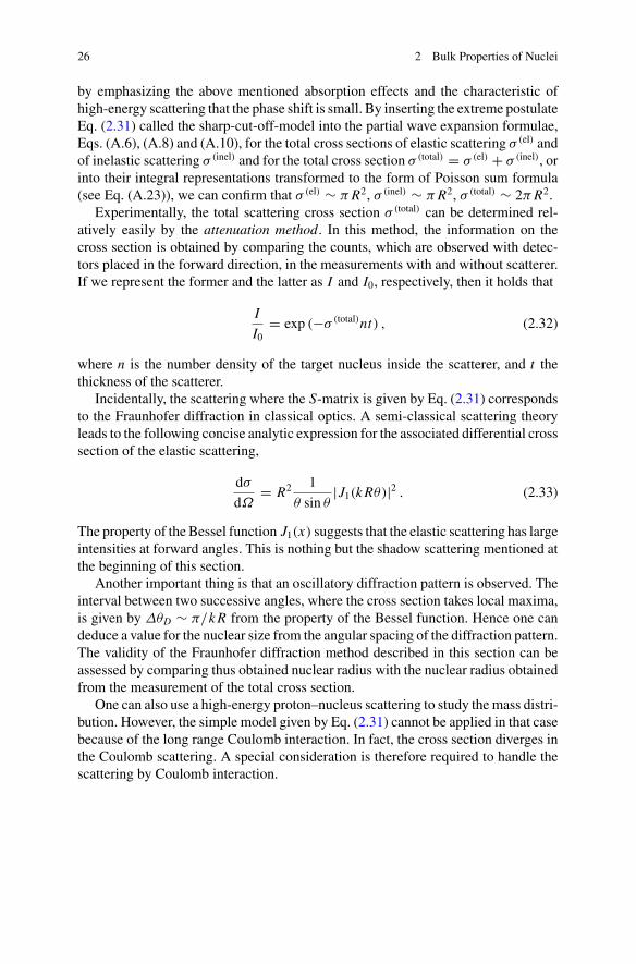
Experimentally, the total scattering cross section σ (total) can be determined rel-atively easily by the attenuation method. In this method, the information on thecross section is obtained by comparing the counts, which are observed with detec-tors placed in the forward direction, in the measurements with and without scatterer.If we represent the former and the latter as I and I0, respectively, then it holds that
I
I0= exp (−σ (total)nt) , (2.32)
where n is the number density of the target nucleus inside the scatterer, and t thethickness of the scatterer.
Incidentally, the scattering where the S-matrix is given by Eq. (2.31) correspondsto the Fraunhofer diffraction in classical optics. A semi-classical scattering theoryleads to the following concise analytic expression for the associated differential crosssection of the elastic scattering,
dσ
dΩ= R2 1
θ sin θ|J1(k Rθ)|2 . (2.33)
The property of the Bessel function J1(x) suggests that the elastic scattering has largeintensities at forward angles. This is nothing but the shadow scattering mentioned atthe beginning of this section.
Another important thing is that an oscillatory diffraction pattern is observed. Theinterval between two successive angles, where the cross section takes local maxima,is given by ΔθD ∼ π/k R from the property of the Bessel function. Hence one candeduce a value for the nuclear size from the angular spacing of the diffraction pattern.The validity of the Fraunhofer diffraction method described in this section can beassessed by comparing thus obtained nuclear radius with the nuclear radius obtainedfrom the measurement of the total cross section.
One can also use a high-energy proton–nucleus scattering to study the mass distri-bution. However, the simple model given by Eq. (2.31) cannot be applied in that casebecause of the long range Coulomb interaction. In fact, the cross section diverges inthe Coulomb scattering. A special consideration is therefore required to handle thescattering by Coulomb interaction.
2.1 Nuclear Sizes 27
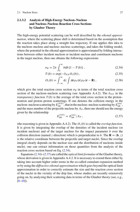
2.1.3.2 Analysis of High-Energy Nucleon–Nucleusand Nucleus–Nucleus Reaction Cross Sectionsby Glauber Theory
The high-energy potential scattering can be well described by the eikonal approxi-mation, where the scattering phase shift is determined based on the assumption thatthe reaction takes place along a straight line trajectory. If one applies this idea tothe nucleon–nucleus and nucleus–nucleus scatterings, and takes the folding model,where the potential in the eikonal approximation is approximated by folding interac-tions between either incident nucleon or incident nucleus and constituent nucleonsin the target nucleus, then one obtains the following expressions
σR = 2π∫ ∞
0bdb [1 − T (b)] , (2.34)
T (b) = exp(−σN N Ov(b)) , (2.35)
Ov(b) =∫ ∞
−∞dz
∫drρT (r)ρP(r − R) , (2.36)
which give the total reaction cross section σR in terms of the total reaction crosssection of the nucleon–nucleon scattering (see Appendix A.4.2). The σN N in thetransparency function T (b) is the average of the total cross section in the proton–neutron and proton–proton scatterings. If one denotes the collision energy in thenucleon–nucleon scattering by E (N N )
lab , that in the nucleus–nucleus scattering by E (nn)lab ,
and the mass number of the projectile nucleus by AP , then one should use the energygiven by the relationship
E (N N )lab = E (nn)
lab /AP , (2.37)
(the reasoning is given in Appendix A.4.2). The Ov(b) is called the overlap function.It is given by integrating the overlap of the densities of the incident nucleus (orincident nucleon) and of the target nucleus for the impact parameter b over thecollision direction (named z-direction) which is perpendicular to b. The R = (b, z)is the relative coordinate between the projectile and target nuclei. Since the overlapintegral clearly depends on the nuclear size and the distribution of nucleons insidenuclei, one can extract information on those quantities from the analysis of thereaction cross section based on Eq. (2.34).
Equations (2.34)–(2.37) are called the optical limit formulae of theGlauber theory,whose derivation is given in Appendix A.4.2. It is necessary to extend them either bytaking into account higher order terms in the so-called cumulant expansion methodor by using the diffractive eikonal approximationwhich goes beyond the optical limitapproximation in order to correctly estimate the size and the reaction cross sectionof the nuclei in the vicinity of the drip line, whose studies are recently extensivelygoing on, by analyzing their scattering data in terms of the Glauber theory (see, e.g.,[8–10]).
28 2 Bulk Properties of Nuclei
2.2 Number Density and Fermi Momentum of Nucleons
2.2.1 Number Density of Nucleons
Let us denote the number density of nucleons inside a nucleus by ρ. Since ρ is definedas the mass number A divided by the volume V , we have
ρ ≡ A
V= 3
4πr30(2.38)
from Eq. (2.27) for spherical nuclei. As Eq. (2.28) shows, the radius parameter r0 isalmost constant independently of the mass number. Equation (2.38) therefore showsthat the number density of nucleons inside a nucleus is almost constant independentlyof individual nucleus. This property is called the density saturation, and is one of theexperimental evidences of the liquid-like behaviour of nuclei leading to the liquid-drop model of nucleus.
2.2.2 Fermi Momentum: Fermi-Gas Model, Thomas–FermiApproximation
One of the simple pictures for the nucleus as a many-body system of nucleons, whichare fermions, is the so-called Fermi-gas model or Thomas–Fermi approximation. Inthat method, each nucleon is considered to be moving independently from each otherin a mean field of volume V . However, the Pauli exclusion principle that each quan-tum state can be occupied by at most only one fermion is respected. Consequently,the nucleons become to distribute from the state of minimum momentum to that ofthe highest momentum called the Fermi momentum. Since there exists one quantumstate for each volume (2π�)3 in the phase space, it holds
A = V
(2π�)3
∫�kF
0p2dpdΩp × 2 × 2 (2.39)
if we represent the Fermi momentum as pF = �kF. The last factor 2 × 2 is the sta-tistical weight in the spin and isospin spaces. Hence we obtain
kF =(3π2
2
)1/3
ρ1/3 =(9π
8
)1/3 1
r0(2.40)
by using Eq. (2.27). Similarly to the density, the Fermi momentum also does notdepend on the mass number. The Fermi wave number is proportional to the 1/3power of the density as one can expect from the consideration of their dimensions.
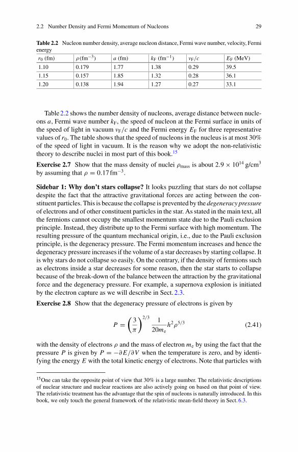
2.2 Number Density and Fermi Momentum of Nucleons 29
Table 2.2 Nucleon number density, average nucleon distance, Fermi wave number, velocity, Fermienergy
r0 (fm) ρ(fm−3) a (fm) kF (fm−1) vF/c EF (MeV)
1.10 0.179 1.77 1.38 0.29 39.5
1.15 0.157 1.85 1.32 0.28 36.1
1.20 0.138 1.94 1.27 0.27 33.1
Table2.2 shows the number density of nucleons, average distance between nucle-ons a, Fermi wave number kF, the speed of nucleon at the Fermi surface in units ofthe speed of light in vacuum vF/c and the Fermi energy EF for three representativevalues of r0. The table shows that the speed of nucleons in the nucleus is at most 30%of the speed of light in vacuum. It is the reason why we adopt the non-relativistictheory to describe nuclei in most part of this book.15
Exercise 2.7 Show that the mass density of nuclei ρmass is about 2.9 × 10¹⁴ g/cm3
by assuming that ρ = 0.17 fm−3.
Sidebar 1: Why don’t stars collapse? It looks puzzling that stars do not collapsedespite the fact that the attractive gravitational forces are acting between the con-stituent particles. This is because the collapse is prevented by the degeneracy pressureof electrons and of other constituent particles in the star. As stated in the main text, allthe fermions cannot occupy the smallest momentum state due to the Pauli exclusionprinciple. Instead, they distribute up to the Fermi surface with high momentum. Theresulting pressure of the quantum mechanical origin, i.e., due to the Pauli exclusionprinciple, is the degeneracy pressure. The Fermi momentum increases and hence thedegeneracy pressure increases if the volume of a star decreases by starting collapse. Itis why stars do not collapse so easily. On the contrary, if the density of fermions suchas electrons inside a star decreases for some reason, then the star starts to collapsebecause of the break-down of the balance between the attraction by the gravitationalforce and the degeneracy pressure. For example, a supernova explosion is initiatedby the electron capture as we will describe in Sect. 2.3.
Exercise 2.8 Show that the degeneracy pressure of electrons is given by
P =(3
π
)2/3 1
20meh2ρ5/3 (2.41)
with the density of electrons ρ and the mass of electron me by using the fact that thepressure P is given by P = −∂ E/∂V when the temperature is zero, and by identi-fying the energy E with the total kinetic energy of electrons. Note that particles with
15One can take the opposite point of view that 30% is a large number. The relativistic descriptionsof nuclear structure and nuclear reactions are also actively going on based on that point of view.The relativistic treatment has the advantage that the spin of nucleons is naturally introduced. In thisbook, we only touch the general framework of the relativistic mean-field theory in Sect. 6.3.
30 2 Bulk Properties of Nuclei
smaller mass work more effectively, i.e., give larger contribution, to the degeneracypressure if the number densities of different particles are the same as Eq. (2.41)shows.
Sidebar 2: Why don’t atoms collapse? A similar question arises for the size ofatoms. Let us consider the neutral hydrogen atom as the example. The attractiveCoulomb force acts between the proton and the electron in the hydrogen atom. Thecorresponding potential energy is given by V (r) = VC(r) = −e2/r when they areseparated by the distance r . It therefore looks energetically most stable at r = 0, i.e.,when the proton and the electron stick to each other. Nonetheless, the size of theHydrogen atom is known to be the Bohr radius given by aB = 0.5 × 10⁻⁸ cm, whichis larger than the radius of proton Rp ∼ 0.8 × 10−13 cm by 5 orders of magnitude.This is also a consequence of quantummechanics. The world of quantummechanics,i.e., the microscopic world, is governed by the uncertainty principle ΔxαΔpα � �.On the other hand, the Hamiltonian describing the motion of the electron aroundthe proton is given by H = p2
2μ + VC(r). Therefore, the uncertainty relation leads to
approximately E � �2
2μ( 1r )2 − e2
r for the corresponding energy. The kinetic energyincreases when r decreases and cancels the gain of the Coulomb energy, and evenleads to a positive total energy. The radius of the Hydrogen atom, i.e., the Bohr radiusaB, is obtained as the value of r which minimizes the energy E .
Sidebar 3: Atoms should have collapsed if the uncertainty principle or the com-mutation relation were absent Since the uncertainty principle is derived from thecommutation relation [xα, pβ ] = i�δαβ , where O is the operator corresponding to anobservable O , atoms would become point particles if the commutation relation didnot govern the nature.
Sidebar 4: Application to Screening Effect As we learnt in Sect. 1.4 concerningthe nuclear reactions in the Sun, many nuclear reactions in stars occur by quantumtunneling through the potential barrier called the Coulomb barrier made by the long-range Coulomb interaction. An interesting phenomenon in this connection is thescreening effect caused by the surrounding charged particles which are in the plasmastate in hot stars. It leads to an enhancement of the tunneling effect. Recently, thescreening effect is argued also in connection with laboratory experiments, wherelow-energy nuclear reactions are caused in matter, e.g., in host metals [11]. It isreported that the reaction rate is enhanced and the screening effect is considered tobe one of the origins of the enhancement. The interest is whether the enhancementof the reaction rate by the screening effect due to the presence of the host material islarge and can explain the observed enhancement [12].
Let us denote the effective Coulomb potential, i.e., the screened Coulomb poten-tial, around a nucleus with electric charge Ze by ϕ(r). If we represent the change ofthe density of a charged particle ζ with the electric charge Zζ e in the surroundinginduced by this nucleus as δρζ (r), then ϕ(r) obeys the Poisson equation
2.2 Number Density and Fermi Momentum of Nucleons 31
Δϕ(r) = −4π
⎡⎣Zeδ(r) +
∑ζ
Zζ eδρζ (r)
⎤⎦ . (2.42)
The nuclear reactions in matter at laboratories are performed at the room tem-perature. Hence, we can use the Thomas–Fermi approximation for the density ofelectrons of the host material, and obtain
ϕ(r) = Ze
rexp(−qTFr) (2.43)
for the solution of Eq. (2.42) within the framework of the linear approximation,where the inverse of the screening length qTF is given by
qTF =√6πρ0
ε(0)F
e2 . (2.44)
The ρ0 and ε(0)F are the density of free electrons in the metal and the Fermi energy,
respectively, before they are polarized.On the other hand, for nuclear reactions in hot stars, the densities of the charged
particles composing the plasma are well represented by the Boltzmann distribution.Consequently, the screened potential is given by the following well-known Debye–Hückel formula,
ϕ(r) = Ze
rexp(−κDHr) , (2.45)
κDH =√4πβe2
∑ζ
Z2ζ ρ
(0)ζ , (2.46)
where β = 1/kT , where k and T are the Boltzmann constant and the temperatureof the star, respectively.
Exercise 2.9 Derive Eqs. (2.44) and (2.46).
2.3 Nuclear Masses
We denote the mass of the nucleus with the mass number A and the atomic numberZ by M(A, Z). The nuclear mass is one of the basic quantities of each nucleus. Atthe same time, it is a fundamental quantity which governs various nuclear reactions.
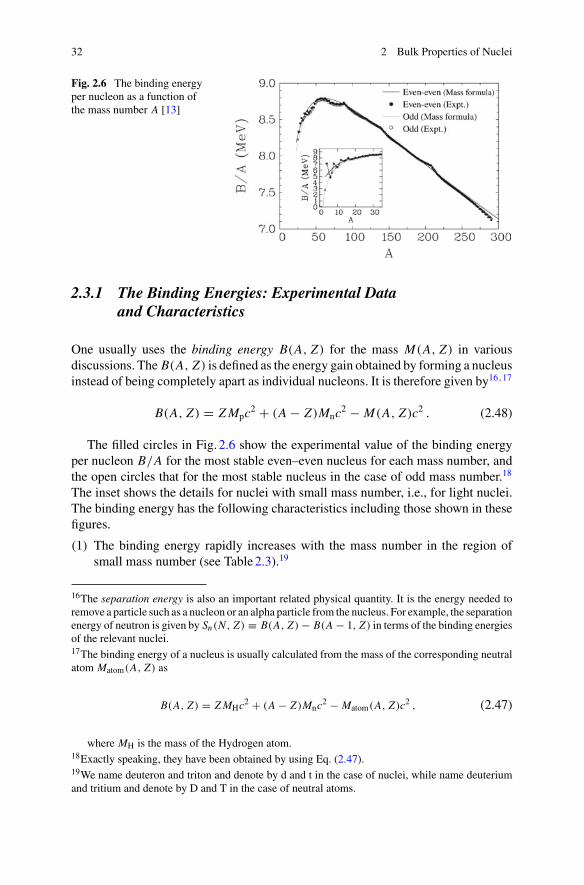
32 2 Bulk Properties of Nuclei
Fig. 2.6 The binding energyper nucleon as a function ofthe mass number A [13]
2.3.1 The Binding Energies: Experimental Dataand Characteristics
One usually uses the binding energy B(A, Z) for the mass M(A, Z) in variousdiscussions. The B(A, Z) is defined as the energy gain obtained by forming a nucleusinstead of being completely apart as individual nucleons. It is therefore given by16,17
B(A, Z) = Z Mpc2 + (A − Z)Mnc2 − M(A, Z)c2 . (2.48)
The filled circles in Fig. 2.6 show the experimental value of the binding energyper nucleon B/A for the most stable even–even nucleus for each mass number, andthe open circles that for the most stable nucleus in the case of odd mass number.18
The inset shows the details for nuclei with small mass number, i.e., for light nuclei.The binding energy has the following characteristics including those shown in thesefigures.
(1) The binding energy rapidly increases with the mass number in the region ofsmall mass number (see Table2.3).19
16The separation energy is also an important related physical quantity. It is the energy needed toremove a particle such as a nucleon or an alpha particle from the nucleus. For example, the separationenergy of neutron is given by Sn(N , Z) ≡ B(A, Z) − B(A − 1, Z) in terms of the binding energiesof the relevant nuclei.17The binding energy of a nucleus is usually calculated from the mass of the corresponding neutralatom Matom(A, Z) as
B(A, Z) = Z MHc2 + (A − Z)Mnc2 − Matom(A, Z)c2 , (2.47)
where MH is the mass of the Hydrogen atom.18Exactly speaking, they have been obtained by using Eq. (2.47).19We name deuteron and triton and denote by d and t in the case of nuclei, while name deuteriumand tritium and denote by D and T in the case of neutral atoms.
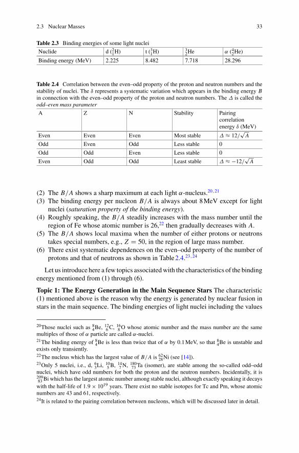
2.3 Nuclear Masses 33
Table 2.3 Binding energies of some light nuclei
Nuclide d (21H) t (31H)32He α (42He)
Binding energy (MeV) 2.225 8.482 7.718 28.296
Table 2.4 Correlation between the even–odd property of the proton and neutron numbers and thestability of nuclei. The δ represents a systematic variation which appears in the binding energy Bin connection with the even–odd property of the proton and neutron numbers. The Δ is called theodd–even mass parameter
A Z N Stability Pairingcorrelationenergy δ (MeV)
Even Even Even Most stable Δ ≈ 12/√
A
Odd Even Odd Less stable 0
Odd Odd Even Less stable 0
Even Odd Odd Least stable Δ ≈ −12/√
A
(2) The B/A shows a sharp maximum at each light α-nucleus.20,21
(3) The binding energy per nucleon B/A is always about 8MeV except for lightnuclei (saturation property of the binding energy).
(4) Roughly speaking, the B/A steadily increases with the mass number until theregion of Fe whose atomic number is 26,22 then gradually decreases with A.
(5) The B/A shows local maxima when the number of either protons or neutronstakes special numbers, e.g., Z = 50, in the region of large mass number.
(6) There exist systematic dependences on the even–odd property of the number ofprotons and that of neutrons as shown in Table2.4.23,24
Let us introduce here a few topics associatedwith the characteristics of the bindingenergy mentioned from (1) through (6).
Topic 1: The Energy Generation in the Main Sequence Stars The characteristic(1) mentioned above is the reason why the energy is generated by nuclear fusion instars in the main sequence. The binding energies of light nuclei including the values
20Those nuclei such as 84Be,
126 C,
168 O whose atomic number and the mass number are the same
multiples of those of α particle are called α-nuclei.21The binding energy of 8
4Be is less than twice that of α by 0.1MeV, so that 84Be is unstable andexists only transiently.22The nucleus which has the largest value of B/A is 62
28Ni (see [14]).23Only 5 nuclei, i.e., d, 6
3Li,105 B,
147 N,
18073 Ta (isomer), are stable among the so-called odd–odd
nuclei, which have odd numbers for both the proton and the neutron numbers. Incidentally, it is20983 Bi which has the largest atomic number among stable nuclei, although exactly speaking it decayswith the half-life of 1.9 × 10¹⁹ years. There exist no stable isotopes for Tc and Pm, whose atomicnumbers are 43 and 61, respectively.24It is related to the pairing correlation between nucleons, which will be discussed later in detail.
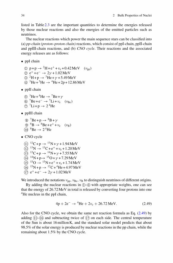
34 2 Bulk Properties of Nuclei
listed in Table2.3 are the important quantities to determine the energies releasedby those nuclear reactions and also the energies of the emitted particles such asneutrinos.
The nuclear reactions which power the main sequence stars can be classified into(a) pp-chain (proton–proton chain) reactions, which consist of ppI-chain, ppII-chainand ppIII-chain reactions, and (b) CNO cycle. Their reactions and the associatedenergy releases are as follows:
• ppI chain
1 p+p → 2H+e+ +νe +0.42MeV (νpp)2 e+ +e− → 2γ +1.02MeV3 2H+p → 3He+γ +5.49MeV4 3He+3He → 4He+2p+12.86MeV
• ppII chain
5 3He+4He → 7Be+γ
6 7Be+e− → 7Li+νe (νBe)7 7Li+p → 2 4He
• ppIII chain
8 7Be+p → 8B+γ
9 8B → 8Be+e+ +νe (νB)10 8Be → 2 4He
• CNO cycle
11 12C+p → 13N+γ +1.94MeV12 13N → 13C+e+ +νe +1.20MeV13 13C+p → 14N+γ +7.55MeV14 14N+p→ 15O+γ +7.29MeV15 15O → 15N+e+ +νe +1.74MeV16 15N+p → 12C+4He+4.97MeV17 e+ +e− → 2γ +1.02MeV
We introduced the notations νpp, νBe, νB to distinguish neutrinos of different origins.By adding the nuclear reactions in 1 – 4 with appropriate weights, one can see
that the energy of 26.72MeV in total is released by converting four protons into one4He nucleus in the ppI chain,
4p + 2e− → 4He + 2νe + 26.72MeV. (2.49)
Also for the CNO cycle, we obtain the same net reaction formula as Eq. (2.49) byadding 11– 16 and subtracting twice of 17 on each side. The central temperatureof the Sun is about 16millionK, and the standard solar model predicts that about98.5% of the solar energy is produced by nuclear reactions in the pp chain, while theremaining about 1.5% by the CNO cycle.
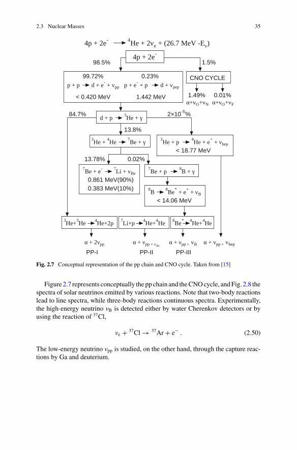
2.3 Nuclear Masses 35
Fig. 2.7 Conceptual representation of the pp chain and CNO cycle. Taken from [15]
Figure2.7 represents conceptually the pp chain and theCNOcycle, andFig. 2.8 thespectra of solar neutrinos emitted by various reactions. Note that two-body reactionslead to line spectra, while three-body reactions continuous spectra. Experimentally,the high-energy neutrino νB is detected either by water Cherenkov detectors or byusing the reaction of 37Cl,
νe + 37Cl → 37Ar + e− . (2.50)
The low-energy neutrino νpp is studied, on the other hand, through the capture reac-tions by Ga and deuterium.
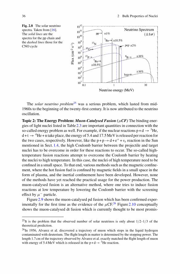
36 2 Bulk Properties of Nuclei
Fig. 2.8 The solar neutrinospectra. Taken from [16].The solid lines are thespectra for the pp chain andthe dashed lines those for theCNO cycle
The solar neutrino problem25 was a serious problem, which lasted from mid-1960s to the beginning of the twenty-first century. It is now attributed to the neutrinooscillation.
Topic 2: The Energy Problem:Muon-Catalysed Fusion (μCF) The binding ener-gies of light nuclei listed in Table2.3 are important quantities in connection with theso-called energy problem as well. For example, if the nuclear reactions p+d → 3He,d+ t → 4He+n take place, the energy of 5.4 and 17.5MeV is released per reaction forthe two cases, respectively. However, like the p+p→d+e+ +νe reaction in the Sunmentioned in Sect. 1.4, the high Coulomb barrier between the projectile and targetnuclei has to be overcome in order for these reactions to occur. The so-called high-temperature fusion reactions attempt to overcome the Coulomb barrier by heatingthe nuclei to high temperature. In this case, the nuclei of high temperature need to beconfined in a small space. To that end, various methods such as the magnetic confine-ment, where the hot fusion fuel is confined by magnetic fields in a small space in theform of plasma, and the inertial confinement have been developed. However, noneof the methods have yet reached the practical usage for the power production. Themuon-catalysed fusion is an alternative method, where one tries to induce fusionreactions at low temperature by lowering the Coulomb barrier with the screeningeffect by μ− particle.
Figure2.9 shows the muon-catalysed pd fusion which has been confirmed exper-imentally for the first time as the evidence of the μCF.26 Figure2.10 conceptuallyshows the muon-catalysed dt fusion which is currently thought to be most promis-
25It is the problem that the observed number of solar neutrinos is only about 1/2–1/3 of thetheoretical prediction.26In 1956, Alvarez et al. discovered a trajectory of muon which stops in the liquid hydrogencontaminated with deuterium. The flight length in matter is determined by the stopping power. Thelength 1.7cm of the trajectory observed by Alvarez et al. exactly matched the flight length of muonwith energy of 5.4MeV which is released in the p+d→ 3He reaction.
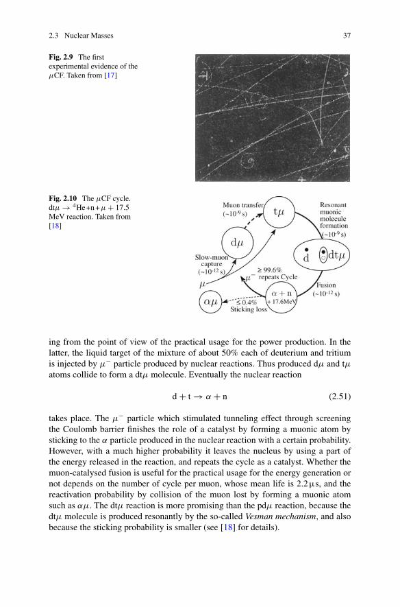
2.3 Nuclear Masses 37
Fig. 2.9 The firstexperimental evidence of theμCF. Taken from [17]
Fig. 2.10 The μCF cycle.dtμ → 4He+n+μ + 17.5MeV reaction. Taken from[18]
ing from the point of view of the practical usage for the power production. In thelatter, the liquid target of the mixture of about 50% each of deuterium and tritiumis injected by μ− particle produced by nuclear reactions. Thus produced dμ and tμatoms collide to form a dtμ molecule. Eventually the nuclear reaction
d + t → α + n (2.51)
takes place. The μ− particle which stimulated tunneling effect through screeningthe Coulomb barrier finishes the role of a catalyst by forming a muonic atom bysticking to the α particle produced in the nuclear reaction with a certain probability.However, with a much higher probability it leaves the nucleus by using a part ofthe energy released in the reaction, and repeats the cycle as a catalyst. Whether themuon-catalysed fusion is useful for the practical usage for the energy generation ornot depends on the number of cycle per muon, whose mean life is 2.2µs, and thereactivation probability by collision of the muon lost by forming a muonic atomsuch as αμ. The dtμ reaction is more promising than the pdμ reaction, because thedtμ molecule is produced resonantly by the so-called Vesman mechanism, and alsobecause the sticking probability is smaller (see [18] for details).
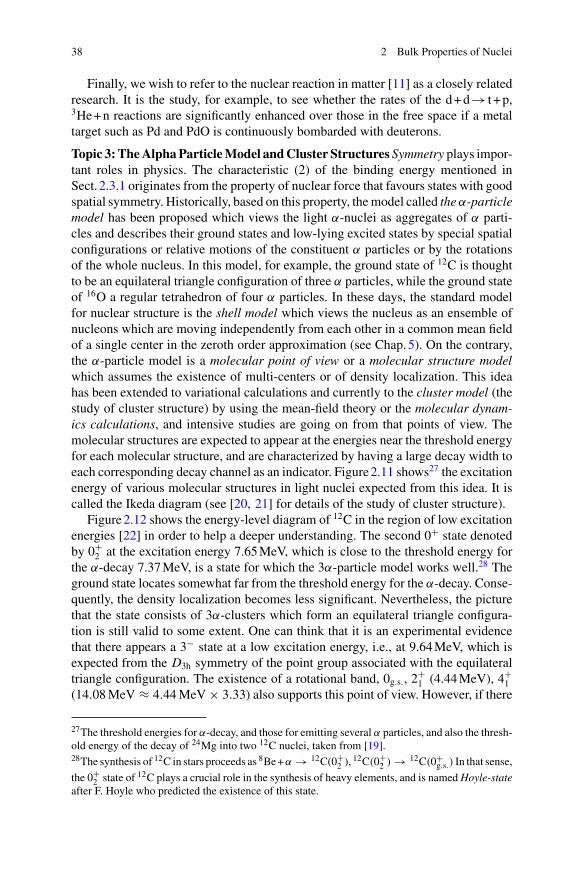
38 2 Bulk Properties of Nuclei
Finally, we wish to refer to the nuclear reaction in matter [11] as a closely relatedresearch. It is the study, for example, to see whether the rates of the d+d→ t +p,3He+n reactions are significantly enhanced over those in the free space if a metaltarget such as Pd and PdO is continuously bombarded with deuterons.
Topic 3:TheAlphaParticleModel andCluster Structures Symmetry plays impor-tant roles in physics. The characteristic (2) of the binding energy mentioned inSect. 2.3.1 originates from the property of nuclear force that favours states with goodspatial symmetry. Historically, based on this property, themodel called the α-particlemodel has been proposed which views the light α-nuclei as aggregates of α parti-cles and describes their ground states and low-lying excited states by special spatialconfigurations or relative motions of the constituent α particles or by the rotationsof the whole nucleus. In this model, for example, the ground state of 12C is thoughtto be an equilateral triangle configuration of three α particles, while the ground stateof 16O a regular tetrahedron of four α particles. In these days, the standard modelfor nuclear structure is the shell model which views the nucleus as an ensemble ofnucleons which are moving independently from each other in a common mean fieldof a single center in the zeroth order approximation (see Chap. 5). On the contrary,the α-particle model is a molecular point of view or a molecular structure modelwhich assumes the existence of multi-centers or of density localization. This ideahas been extended to variational calculations and currently to the cluster model (thestudy of cluster structure) by using the mean-field theory or the molecular dynam-ics calculations, and intensive studies are going on from that points of view. Themolecular structures are expected to appear at the energies near the threshold energyfor each molecular structure, and are characterized by having a large decay width toeach corresponding decay channel as an indicator. Figure2.11 shows27 the excitationenergy of various molecular structures in light nuclei expected from this idea. It iscalled the Ikeda diagram (see [20, 21] for details of the study of cluster structure).
Figure2.12 shows the energy-level diagram of 12C in the region of low excitationenergies [22] in order to help a deeper understanding. The second 0+ state denotedby 0+
2 at the excitation energy 7.65MeV, which is close to the threshold energy forthe α-decay 7.37MeV, is a state for which the 3α-particle model works well.28 Theground state locates somewhat far from the threshold energy for the α-decay. Conse-quently, the density localization becomes less significant. Nevertheless, the picturethat the state consists of 3α-clusters which form an equilateral triangle configura-tion is still valid to some extent. One can think that it is an experimental evidencethat there appears a 3− state at a low excitation energy, i.e., at 9.64MeV, which isexpected from the D3h symmetry of the point group associated with the equilateraltriangle configuration. The existence of a rotational band, 0g.s., 2
+1 (4.44MeV), 4+
1(14.08MeV ≈ 4.44MeV × 3.33) also supports this point of view. However, if there
27The threshold energies for α-decay, and those for emitting several α particles, and also the thresh-old energy of the decay of 24Mg into two 12C nuclei, taken from [19].28The synthesis of 12C in stars proceeds as 8Be+α → 12C(0+
2 ),12C(0+
2 ) → 12C(0+g.s.) In that sense,
the 0+2 state of 12C plays a crucial role in the synthesis of heavy elements, and is named Hoyle-state
after F. Hoyle who predicted the existence of this state.
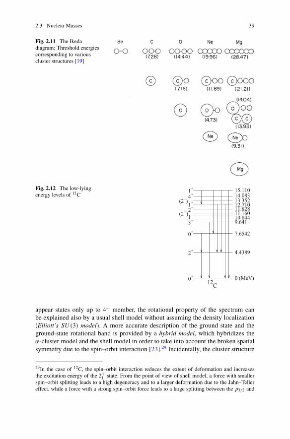
2.3 Nuclear Masses 39
Fig. 2.11 The Ikedadiagram: Threshold energiescorresponding to variouscluster structures [19]
Fig. 2.12 The low-lyingenergy levels of 12C
12C0 (MeV)
4.4389
7.6542
9.64110.84411.16011.82812.71013.35214.08315.110
0+
2+
0+
3–1–(2+)2–1+(2–)4+1+
appear states only up to 4+ member, the rotational property of the spectrum canbe explained also by a usual shell model without assuming the density localization(Elliott’s SU (3) model). A more accurate description of the ground state and theground-state rotational band is provided by a hybrid model, which hybridizes theα-cluster model and the shell model in order to take into account the broken spatialsymmetry due to the spin–orbit interaction [23].29 Incidentally, the cluster structure
29In the case of 12C, the spin–orbit interaction reduces the extent of deformation and increasesthe excitation energy of the 2+
1 state. From the point of view of shell model, a force with smallerspin–orbit splitting leads to a high degeneracy and to a larger deformation due to the Jahn–Tellereffect, while a force with a strong spin–orbit force leads to a large splitting between the p3/2 and
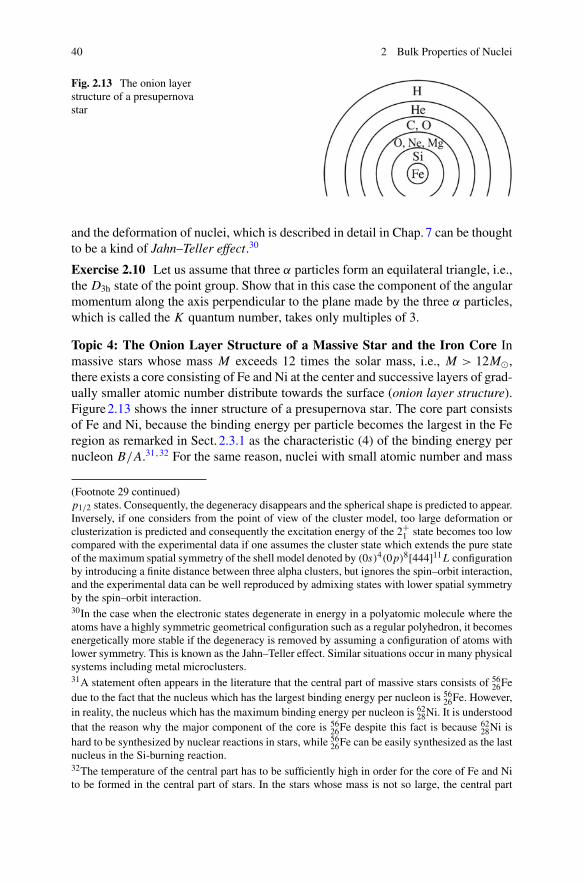
40 2 Bulk Properties of Nuclei
Fig. 2.13 The onion layerstructure of a presupernovastar
and the deformation of nuclei, which is described in detail in Chap. 7 can be thoughtto be a kind of Jahn–Teller effect.30
Exercise 2.10 Let us assume that three α particles form an equilateral triangle, i.e.,the D3h state of the point group. Show that in this case the component of the angularmomentum along the axis perpendicular to the plane made by the three α particles,which is called the K quantum number, takes only multiples of 3.
Topic 4: The Onion Layer Structure of a Massive Star and the Iron Core Inmassive stars whose mass M exceeds 12 times the solar mass, i.e., M > 12M�,there exists a core consisting of Fe and Ni at the center and successive layers of grad-ually smaller atomic number distribute towards the surface (onion layer structure).Figure2.13 shows the inner structure of a presupernova star. The core part consistsof Fe and Ni, because the binding energy per particle becomes the largest in the Feregion as remarked in Sect. 2.3.1 as the characteristic (4) of the binding energy pernucleon B/A.31,32 For the same reason, nuclei with small atomic number and mass
(Footnote 29 continued)p1/2 states. Consequently, the degeneracy disappears and the spherical shape is predicted to appear.Inversely, if one considers from the point of view of the cluster model, too large deformation orclusterization is predicted and consequently the excitation energy of the 2+
1 state becomes too lowcompared with the experimental data if one assumes the cluster state which extends the pure stateof the maximum spatial symmetry of the shell model denoted by (0s)4(0p)8[444]11L configurationby introducing a finite distance between three alpha clusters, but ignores the spin–orbit interaction,and the experimental data can be well reproduced by admixing states with lower spatial symmetryby the spin–orbit interaction.30In the case when the electronic states degenerate in energy in a polyatomic molecule where theatoms have a highly symmetric geometrical configuration such as a regular polyhedron, it becomesenergetically more stable if the degeneracy is removed by assuming a configuration of atoms withlower symmetry. This is known as the Jahn–Teller effect. Similar situations occur in many physicalsystems including metal microclusters.31A statement often appears in the literature that the central part of massive stars consists of 56
26Fedue to the fact that the nucleus which has the largest binding energy per nucleon is 56
26Fe. However,in reality, the nucleus which has the maximum binding energy per nucleon is 62
28Ni. It is understoodthat the reason why the major component of the core is 56
26Fe despite this fact is because 6228Ni is
hard to be synthesized by nuclear reactions in stars, while 5626Fe can be easily synthesized as the last
nucleus in the Si-burning reaction.32The temperature of the central part has to be sufficiently high in order for the core of Fe and Nito be formed in the central part of stars. In the stars whose mass is not so large, the central part
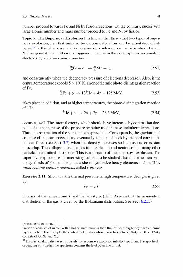
2.3 Nuclear Masses 41
number proceed towards Fe and Ni by fusion reactions. On the contrary, nuclei withlarge atomic number and mass number proceed to Fe and Ni by fission.
Topic 5: The Supernova Explosion It is known that there exist two types of super-nova explosion, i.e., that initiated by carbon detonation and by gravitational col-lapse.33 In the latter case, and in massive stars whose core part is made of Fe andNi, the gravitational collapse is triggered when Fe in the core captures surroundingelectrons by electron capture reaction,
5626Fe + e− → 56
25Mn + νe , (2.52)
and consequently when the degeneracy pressure of electrons decreases. Also, if thecentral temperature exceeds 5 × 10⁹ K, an endothermic photo-disintegration reactionof Fe,
5626Fe + γ → 134He + 4n − 125MeV, (2.53)
takes place in addition, and at higher temperatures, the photo-disintegration reactionof 4He,
4He + γ → 2n + 2p − 28.3MeV, (2.54)
occurs as well. The internal energy which should have increased by contraction doesnot lead to the increase of the pressure by being used in these endothermic reactions.Thus, the contraction of the star cannot be prevented. Consequently, the gravitationalcollapse of the star proceeds and eventually is bounced back by the hard core in thenuclear force (see Sect. 3.7) when the density increases so high as nucleons startto overlap. The collapse thus changes into explosion and neutrinos and many otherparticles are emitted into space. This is a scenario of the supernova explosion. Thesupernova explosion is an interesting subject to be studied also in connection withthe synthesis of elements, e.g., as a site to synthesize heavy elements such as U byrapid neutron capture reactions called r-process.
Exercise 2.11 Show that the thermal pressure in high temperature ideal gas is givenby
PT = ρT (2.55)
in terms of the temperature T and the density ρ. (Hint: Assume that the momentumdistribution of the gas is given by the Boltzmann distribution. See Sect. 6.2.5.)
(Footnote 32 continued)therefore consists of nuclei with smaller mass number than that of Fe, though they have an onionlayer structure. For example, the central part of stars whose mass lies between 8M� < M < 12M�consists of O, Ne and Mg.33There is an alternative way to classify the supernova explosion into the type II and I, respectively,depending on whether the spectrum contains the hydrogen line or not.
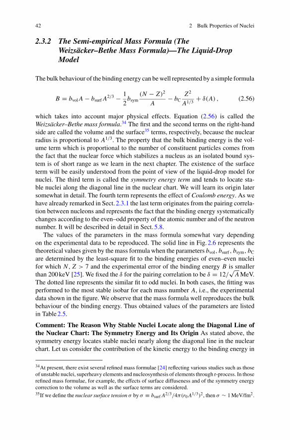
42 2 Bulk Properties of Nuclei
2.3.2 The Semi-empirical Mass Formula (TheWeizsäcker–Bethe Mass Formula)—The Liquid-DropModel
The bulk behaviour of the binding energy can bewell represented by a simple formula
B = bvol A − bsurf A2/3 − 1
2bsym
(N − Z)2
A− bC
Z2
A1/3+ δ(A) , (2.56)
which takes into account major physical effects. Equation (2.56) is called theWeizsäcker–Bethe mass formula.34 The first and the second terms on the right-handside are called the volume and the surface35 terms, respectively, because the nuclearradius is proportional to A1/3. The property that the bulk binding energy is the vol-ume term which is proportional to the number of constituent particles comes fromthe fact that the nuclear force which stabilizes a nucleus as an isolated bound sys-tem is of short range as we learn in the next chapter. The existence of the surfaceterm will be easily understood from the point of view of the liquid-drop model fornuclei. The third term is called the symmetry energy term and tends to locate sta-ble nuclei along the diagonal line in the nuclear chart. We will learn its origin latersomewhat in detail. The fourth term represents the effect of Coulomb energy. As wehave already remarked in Sect. 2.3.1 the last term originates from the pairing correla-tion between nucleons and represents the fact that the binding energy systematicallychanges according to the even–odd property of the atomic number and of the neutronnumber. It will be described in detail in Sect. 5.8.
The values of the parameters in the mass formula somewhat vary dependingon the experimental data to be reproduced. The solid line in Fig. 2.6 represents thetheoretical values given by themass formula when the parameters bvol, bsurf , bsym, bCare determined by the least-square fit to the binding energies of even–even nucleifor which N , Z > 7 and the experimental error of the binding energy B is smallerthan 200keV [25]. We fixed the δ for the pairing correlation to be δ = 12/
√AMeV.
The dotted line represents the similar fit to odd nuclei. In both cases, the fitting wasperformed to the most stable isobar for each mass number A, i.e., the experimentaldata shown in the figure. We observe that the mass formula well reproduces the bulkbehaviour of the binding energy. Thus obtained values of the parameters are listedin Table2.5.
Comment: The Reason Why Stable Nuclei Locate along the Diagonal Line ofthe Nuclear Chart: The Symmetry Energy and Its Origin As stated above, thesymmetry energy locates stable nuclei nearly along the diagonal line in the nuclearchart. Let us consider the contribution of the kinetic energy to the binding energy in
34At present, there exist several refined mass formulae [24] reflecting various studies such as thoseof unstable nuclei, superheavy elements and nucleosynthesis of elements through r-process. In thoserefined mass formulae, for example, the effects of surface diffuseness and of the symmetry energycorrection to the volume as well as the surface terms are considered.35If we define the nuclear surface tension σ by σ ≡ bsurf A2/3/4π(r0 A1/3)2, then σ ∼ 1MeV/fm2.
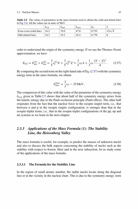
2.3 Nuclear Masses 43
Table 2.5 The values of parameters in the mass formula used to obtain the solid and dotted linesin Fig. 2.6. All the values are in units of MeV
bvol bsurf bsym bC δ
Even–even (solid line) 16.2 19.0 47.0 0.755 12/√
A
Odd (dotted line) 16.3 19.2 45.4 0.770 0
order to understand the origin of the symmetry energy. If we use the Thomas–Fermiapproximation, we have
Ekin = E (n)kin + E (p)
kin = 3
5ε
(n)F N + 3
5ε
(p)F Z ≈ 3
5εF A + 1
3εF
(N − Z)2
A. (2.57)
By comparing the second term on the right-hand side of Eq. (2.57) with the symmetryenergy term in the mass formula, we obtain
b(kin)sym = 2
3εF ∼ 25MeV. (2.58)
The comparison of this value with the value of the parameter of the symmetry energybsym given in Table2.5 shows that about half of the symmetry energy arises fromthe kinetic energy due to the Pauli exclusion principle (Pauli effect). The other halforiginates from the fact that the nuclear force in the isospin singlet term, i.e., thatbetween n and p in the isospin singlet configuration, is stronger than that in theisospin triplet terms, i.e., that in the isospin triplet configurations of the pp, np andnn systems as we learn in the next chapter.
2.3.3 Applications of the Mass Formula (1): The StabilityLine, the Heisenberg Valley
The mass formula is useful, for example, to predict the masses of unknown nucleiand also to discuss the bulk aspects concerning the stability of nuclei such as thestability with respect to fission. Here and in the next subsection, let us study someof the applications of the mass formula.
2.3.3.1 The Formula for the Stability Line
In the region of small atomic number, the stable nuclei locate along the diagonalline or in the vicinity in the nuclear chart. This is due to the symmetry energy term
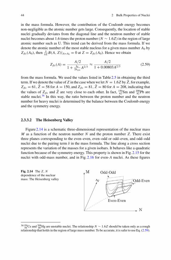
44 2 Bulk Properties of Nuclei
in the mass formula. However, the contribution of the Coulomb energy becomesnon-negligible as the atomic number gets large. Consequently, the location of stablenuclei gradually deviates from the diagonal line and the neutron number of stablenuclei becomes about 1.6 times the proton number (N ∼ 1.6Z ) in the region of largeatomic number such as U. This trend can be derived from the mass formula. If wedenote the atomic number of the most stable nucleus for a given mass number A0 byZβs(A0), then ∂
∂ Z B(A, Z)|A=A0 = 0 at Z = Zβs(A0). Hence we obtain
Zβs(A) = A/2
1 + bC2bsym
A2/3≈ A/2
1 + 0.00803A2/3(2.59)
from the mass formula. We used the values listed in Table2.5 in obtaining the thirdterm. Ifwe denote the value of Z in the casewhenwe let N = 1.6Z by Z , for example,Zβs = 61, Z = 58 for A = 150, and Zβs = 81, Z = 80 for A = 208, indicating thatthe values of Zβs and Z are very close to each other. In fact, 15062 Sm and 208
82 Pb arestable nuclei.36 In this way, the ratio between the proton number and the neutronnumber for heavy nuclei is determined by the balance between the Coulomb energyand the symmetry energy.
2.3.3.2 The Heisenberg Valley
Figure2.14 is a schematic three-dimensional representation of the nuclear massM as a function of the neutron number N and the proton number Z . There existthree planes corresponding to the even–even, even–odd or odd–even, and odd–oddnuclei due to the pairing term δ in the mass formula. The line along a cross sectionrepresents the variation of the masses for a given isobars. It behaves like a quadraticfunction because of the symmetry energy. This property is shown in Fig. 2.15 for thenuclei with odd-mass number, and in Fig. 2.16 for even-A nuclei. As these figures
Fig. 2.14 The Z , Ndependence of the nuclearmass: The Heisenberg valley
3615058 Ce and
20880 Hg are unstable nuclei. The relationship N ∼ 1.6Z should be taken only as a rough
relationship that holds in the region of largemass number. To be accurate, it is safer to use Eq. (2.59).
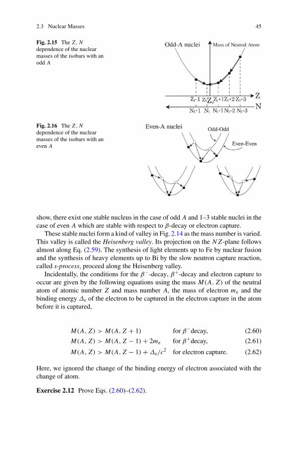
2.3 Nuclear Masses 45
Fig. 2.15 The Z , Ndependence of the nuclearmasses of the isobars with anodd A
Fig. 2.16 The Z , Ndependence of the nuclearmasses of the isobars with aneven A
show, there exist one stable nucleus in the case of odd A and 1–3 stable nuclei in thecase of even A which are stable with respect to β-decay or electron capture.
These stable nuclei form a kind of valley in Fig. 2.14 as the mass number is varied.This valley is called the Heisenberg valley. Its projection on the N Z -plane followsalmost along Eq. (2.59). The synthesis of light elements up to Fe by nuclear fusionand the synthesis of heavy elements up to Bi by the slow neutron capture reaction,called s-process, proceed along the Heisenberg valley.
Incidentally, the conditions for the β−-decay, β+-decay and electron capture tooccur are given by the following equations using the mass M(A, Z) of the neutralatom of atomic number Z and mass number A, the mass of electron me and thebinding energy Δe of the electron to be captured in the electron capture in the atombefore it is captured,
M(A, Z) > M(A, Z + 1) for β−decay, (2.60)
M(A, Z) > M(A, Z − 1) + 2me for β+decay, (2.61)
M(A, Z) > M(A, Z − 1) + Δe/c2 for electron capture. (2.62)
Here, we ignored the change of the binding energy of electron associated with thechange of atom.
Exercise 2.12 Prove Eqs. (2.60)–(2.62).
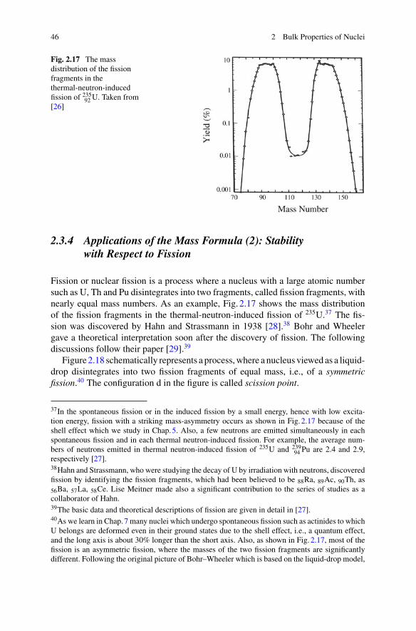
46 2 Bulk Properties of Nuclei
Fig. 2.17 The massdistribution of the fissionfragments in thethermal-neutron-inducedfission of 23592 U. Taken from[26]
2.3.4 Applications of the Mass Formula (2): Stabilitywith Respect to Fission
Fission or nuclear fission is a process where a nucleus with a large atomic numbersuch as U, Th and Pu disintegrates into two fragments, called fission fragments, withnearly equal mass numbers. As an example, Fig. 2.17 shows the mass distributionof the fission fragments in the thermal-neutron-induced fission of 235U.37 The fis-sion was discovered by Hahn and Strassmann in 1938 [28].38 Bohr and Wheelergave a theoretical interpretation soon after the discovery of fission. The followingdiscussions follow their paper [29].39
Figure2.18 schematically represents a process,where a nucleus viewed as a liquid-drop disintegrates into two fission fragments of equal mass, i.e., of a symmetricfission.40 The configuration d in the figure is called scission point.
37In the spontaneous fission or in the induced fission by a small energy, hence with low excita-tion energy, fission with a striking mass-asymmetry occurs as shown in Fig. 2.17 because of theshell effect which we study in Chap.5. Also, a few neutrons are emitted simultaneously in eachspontaneous fission and in each thermal neutron-induced fission. For example, the average num-bers of neutrons emitted in thermal neutron-induced fission of 235U and 239
94 Pu are 2.4 and 2.9,respectively [27].38Hahn and Strassmann, who were studying the decay of U by irradiation with neutrons, discoveredfission by identifying the fission fragments, which had been believed to be 88Ra, 89Ac, 90Th, as56Ba, 57La, 58Ce. Lise Meitner made also a significant contribution to the series of studies as acollaborator of Hahn.39The basic data and theoretical descriptions of fission are given in detail in [27].40As we learn in Chap.7 many nuclei which undergo spontaneous fission such as actinides to whichU belongs are deformed even in their ground states due to the shell effect, i.e., a quantum effect,and the long axis is about 30% longer than the short axis. Also, as shown in Fig. 2.17, most of thefission is an asymmetric fission, where the masses of the two fission fragments are significantlydifferent. Following the original picture of Bohr–Wheeler which is based on the liquid-drop model,
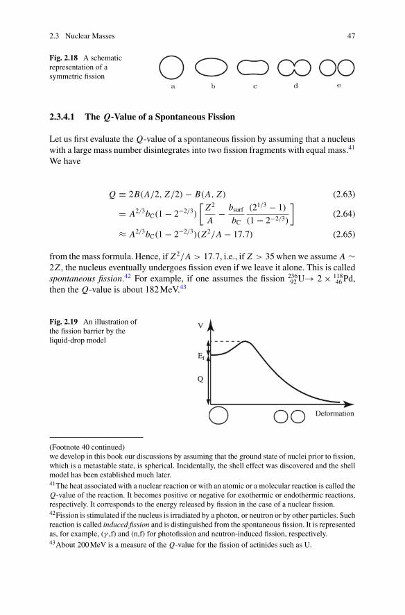
2.3 Nuclear Masses 47
Fig. 2.18 A schematicrepresentation of asymmetric fission
2.3.4.1 The Q-Value of a Spontaneous Fission
Let us first evaluate the Q-value of a spontaneous fission by assuming that a nucleuswith a large mass number disintegrates into two fission fragments with equal mass.41
We have
Q ≡ 2B(A/2, Z/2) − B(A, Z) (2.63)
= A2/3bC(1 − 2−2/3)
[Z2
A− bsurf
bC
(21/3 − 1)
(1 − 2−2/3)
](2.64)
≈ A2/3bC(1 − 2−2/3)(Z2/A − 17.7) (2.65)
from themass formula. Hence, if Z2/A > 17.7, i.e., if Z > 35when we assume A ∼2Z , the nucleus eventually undergoes fission even if we leave it alone. This is calledspontaneous fission.42 For example, if one assumes the fission 236
92U→ 2 × 11846 Pd,
then the Q-value is about 182MeV.43
Fig. 2.19 An illustration ofthe fission barrier by theliquid-drop model
(Footnote 40 continued)we develop in this book our discussions by assuming that the ground state of nuclei prior to fission,which is a metastable state, is spherical. Incidentally, the shell effect was discovered and the shellmodel has been established much later.41The heat associated with a nuclear reaction or with an atomic or a molecular reaction is called theQ-value of the reaction. It becomes positive or negative for exothermic or endothermic reactions,respectively. It corresponds to the energy released by fission in the case of a nuclear fission.42Fission is stimulated if the nucleus is irradiated by a photon, or neutron or by other particles. Suchreaction is called induced fission and is distinguished from the spontaneous fission. It is representedas, for example, (γ ,f) and (n,f) for photofission and neutron-induced fission, respectively.43About 200MeV is a measure of the Q-value for the fission of actinides such as U.
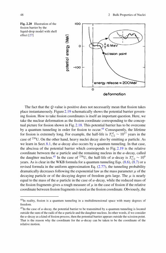
48 2 Bulk Properties of Nuclei
Fig. 2.20 Illustration of thefission barrier by theliquid-drop model with shelleffect [27]
The fact that the Q-value is positive does not necessarily mean that fission takesplace instantaneously. Figure2.19 schematically shows the potential barrier govern-ing fission. How to take fission coordinates is itself an important question. Here, wetake the nuclear deformation as the fission coordinate corresponding to the concep-tual picture for fission shown in Fig. 2.18. This potential barrier has to be overcomeby a quantum tunneling in order for fission to occur.44 Consequently, the lifetimefor fission is extremely long. For example, the half-life is T sf
1/2 ∼ 1017 years in thecase of 238U. On the other hand, heavy nuclei decay also by emitting α particle. Aswe learn in Sect. 8.1, the α-decay also occurs by a quantum tunneling. In that case,the abscissa of the potential barrier which corresponds to Fig. 2.19 is the relativecoordinate between the α particle and the remaining nucleus in the α-decay, calledthe daughter nucleus.45 In the case of 238U, the half-life of α-decay is T α
1/2 ∼ 109
years. As is clear in the WKB formula for a quantum tunneling Eqs. (8.6), (8.7) or arevised formula in the uniform approximation Eq. (2.77), the tunneling probabilitydramatically decreases following the exponential law as the mass parameter μ of thedecaying particle or of the decaying degree of freedom gets large. The μ is nearlyequal to the mass of the α particle in the case of α-decay, while the reduced mass ofthe fission fragments gives a rough measure of μ in the case of fission if the relativecoordinate between fission fragments is used as the fission coordinate. Obviously, the
44In reality, fission is a quantum tunneling in a multidimensional space with many degrees offreedom.45In the case of α-decay, the potential barrier to be transmitted by a quantum tunneling is locatedoutside the sum of the radii of the α particle and the daughter nucleus. In other words, if we considerthe α-decay as a kind of fission process, then the potential barrier appears outside the scission point.That is the reason why the coordinate for the α-decay can be taken to be the coordinate of therelative motion.
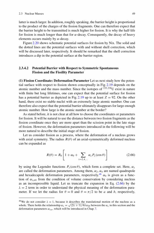
2.3 Nuclear Masses 49
latter is much larger. In addition, roughly speaking, the barrier height is proportionalto the product of the charges of the fission fragments. One can therefore expect thatthe barrier height to be transmitted is much higher for fission. It is why the half-lifefor fission is much longer than that for α-decay. Consequently, the decay of heavyelements occurs mainly by α-decay.
Figure2.20 shows schematic potential surfaces for fission by Nix. The solid andthe dotted lines are the potential surfaces with and without shell correction, whichwill be discussed later, respectively. It should be remarked that the shell correctionintroduces a dip in the potential surface at the barrier region.
2.3.4.2 Potential Barrier with Respect to Symmetric SpontaneousFission and the Fissility Parameter
(1) Fission Coordinate: Deformation Parameter Let us next study how the poten-tial surface with respect to fission shown conceptually in Fig. 2.19 depends on theatomic number and the mass number. Since the isotopes of 235,238U exist in naturewith finite but long lifetimes, one can expect that the potential surface for fissionhas a potential barrier as depicted in Fig. 2.19 up to at least Z = 92. On the otherhand, there exist no stable nuclei with an extremely large atomic number. One cantherefore also expect that the potential barrier ultimately disappears for large enoughatomic number. How large is the atomic number at the border?
As stated before, it is not clear at all how to choose the coordinates or parametersfor fission. It will be natural to use the distance between two fission fragments as thefission coordinate once they are more apart than the scission point in the late stageof fission. However, the deformation parameters introduced in the following will bemore natural to describe the initial stage of fission.
Let us consider fission as a process, where the deformation of a nucleus growswith axial symmetry. The radius R(θ) of an axial-symmetrically deformed nucleuscan be expanded as
R(θ) = R0
[1 + α0 +
∑λ=2,4,...
αλ Pλ(cos θ)
](2.66)
by using the Legendre functions Pλ(cos θ), which form a complete set. Here, αλ
are called the deformation parameters. Among them, α2, α4 are named quadrupoleand hexadecapole deformation parameters, respectively.46 α0 is given as a func-tion of αλ =0 from the condition of volume conservation by considering nucleusas an incompressible liquid. Let us truncate the expansion in Eq. (2.66) by theλ = 2 term in order to understand the physical meaning of the deformation para-meter. If we let the radius for θ = 0 and θ = π/2 to be a and b, respectively,
46We do not consider λ = 1, because it describes the translational motion of the nucleus as awhole. There holds the relationship αλ = √
(2λ + 1)/4πα20 between the αλ in this section and thedeformation parameters αλμ, which will be introduced in Chap.7.
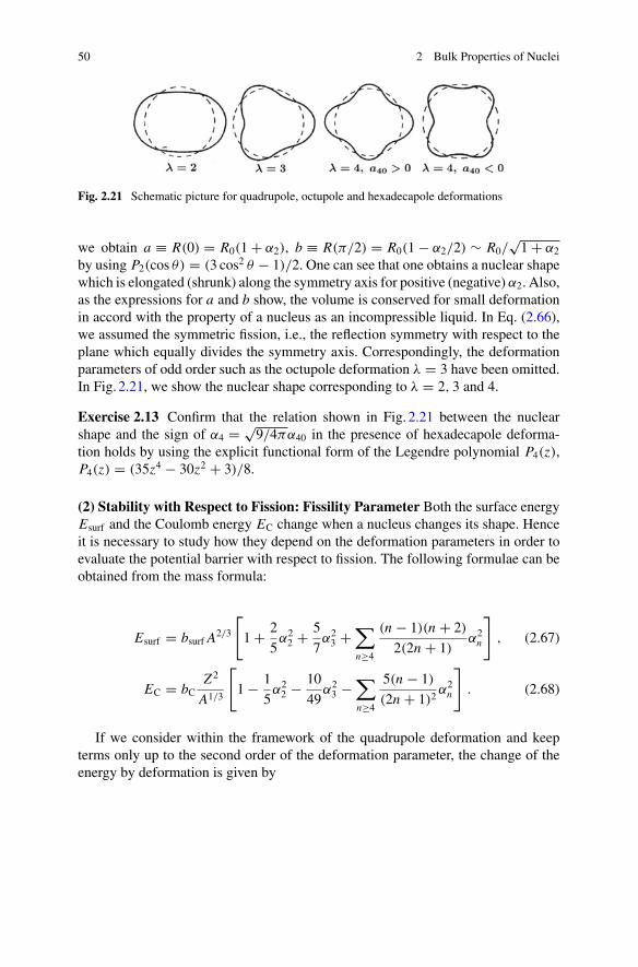
50 2 Bulk Properties of Nuclei
Fig. 2.21 Schematic picture for quadrupole, octupole and hexadecapole deformations
we obtain a ≡ R(0) = R0(1 + α2), b ≡ R(π/2) = R0(1 − α2/2) ∼ R0/√1 + α2
by using P2(cos θ) = (3 cos2 θ − 1)/2. One can see that one obtains a nuclear shapewhich is elongated (shrunk) along the symmetry axis for positive (negative) α2. Also,as the expressions for a and b show, the volume is conserved for small deformationin accord with the property of a nucleus as an incompressible liquid. In Eq. (2.66),we assumed the symmetric fission, i.e., the reflection symmetry with respect to theplane which equally divides the symmetry axis. Correspondingly, the deformationparameters of odd order such as the octupole deformation λ = 3 have been omitted.In Fig. 2.21, we show the nuclear shape corresponding to λ = 2, 3 and 4.
Exercise 2.13 Confirm that the relation shown in Fig. 2.21 between the nuclearshape and the sign of α4 = √
9/4πα40 in the presence of hexadecapole deforma-tion holds by using the explicit functional form of the Legendre polynomial P4(z),P4(z) = (35z4 − 30z2 + 3)/8.
(2) Stability with Respect to Fission: Fissility Parameter Both the surface energyEsurf and the Coulomb energy EC change when a nucleus changes its shape. Henceit is necessary to study how they depend on the deformation parameters in order toevaluate the potential barrier with respect to fission. The following formulae can beobtained from the mass formula:
Esurf = bsurf A2/3
[1 + 2
5α22 + 5
7α23 +
∑n≥4
(n − 1)(n + 2)
2(2n + 1)α2
n
], (2.67)
EC = bCZ2
A1/3
[1 − 1
5α22 − 10
49α23 −
∑n≥4
5(n − 1)
(2n + 1)2α2
n
]. (2.68)
If we consider within the framework of the quadrupole deformation and keepterms only up to the second order of the deformation parameter, the change of theenergy by deformation is given by
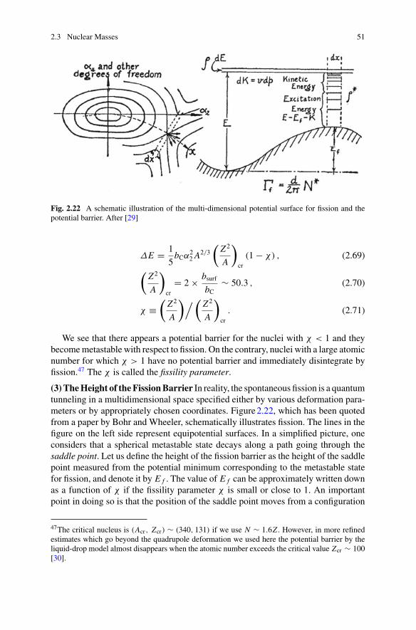
2.3 Nuclear Masses 51
Fig. 2.22 A schematic illustration of the multi-dimensional potential surface for fission and thepotential barrier. After [29]
ΔE = 1
5bCα2
2 A2/3
(Z2
A
)cr
(1 − χ) , (2.69)
(Z2
A
)cr
= 2 × bsurfbC
∼ 50.3 , (2.70)
χ ≡(
Z2
A
)/ (Z2
A
)cr
. (2.71)
We see that there appears a potential barrier for the nuclei with χ < 1 and theybecomemetastable with respect to fission. On the contrary, nuclei with a large atomicnumber for which χ > 1 have no potential barrier and immediately disintegrate byfission.47 The χ is called the fissility parameter.
(3) TheHeight of theFissionBarrier In reality, the spontaneous fission is a quantumtunneling in a multidimensional space specified either by various deformation para-meters or by appropriately chosen coordinates. Figure2.22, which has been quotedfrom a paper by Bohr and Wheeler, schematically illustrates fission. The lines in thefigure on the left side represent equipotential surfaces. In a simplified picture, oneconsiders that a spherical metastable state decays along a path going through thesaddle point. Let us define the height of the fission barrier as the height of the saddlepoint measured from the potential minimum corresponding to the metastable statefor fission, and denote it by E f . The value of E f can be approximately written downas a function of χ if the fissility parameter χ is small or close to 1. An importantpoint in doing so is that the position of the saddle point moves from a configuration
47The critical nucleus is (Acr, Zcr) ∼ (340, 131) if we use N ∼ 1.6Z . However, in more refinedestimates which go beyond the quadrupole deformation we used here the potential barrier by theliquid-drop model almost disappears when the atomic number exceeds the critical value Zcr ∼ 100[30].
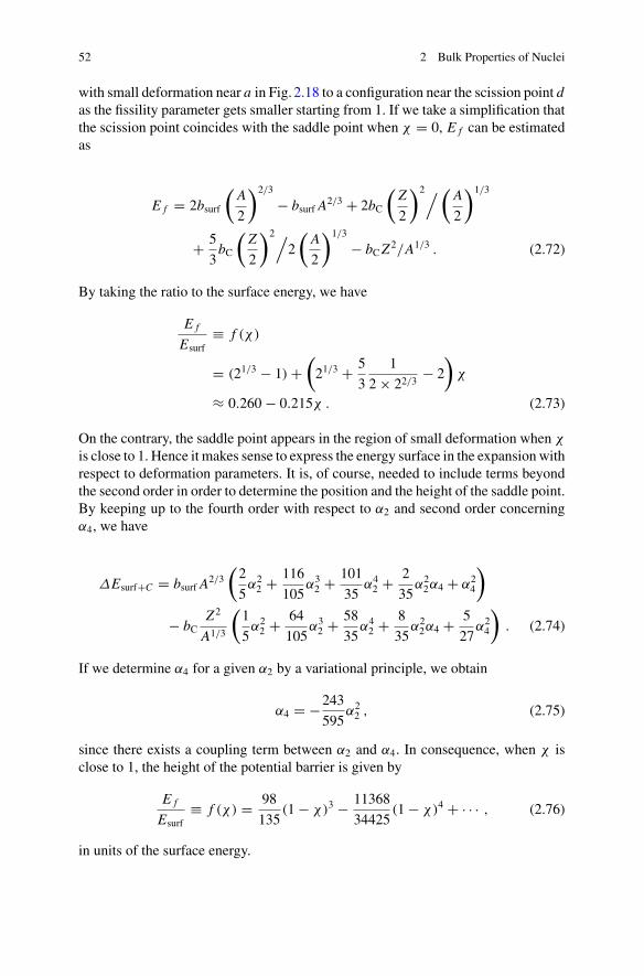
52 2 Bulk Properties of Nuclei
with small deformation near a in Fig. 2.18 to a configuration near the scission point das the fissility parameter gets smaller starting from 1. If we take a simplification thatthe scission point coincides with the saddle point when χ = 0, E f can be estimatedas
E f = 2bsurf
(A
2
)2/3
− bsurf A2/3 + 2bC
(Z
2
)2/ (A
2
)1/3
+ 5
3bC
(Z
2
)2/2
(A
2
)1/3
− bCZ2/A1/3 . (2.72)
By taking the ratio to the surface energy, we have
E f
Esurf≡ f (χ)
= (21/3 − 1) +(21/3 + 5
3
1
2 × 22/3− 2
)χ
≈ 0.260 − 0.215χ . (2.73)
On the contrary, the saddle point appears in the region of small deformation when χ
is close to 1. Hence it makes sense to express the energy surface in the expansion withrespect to deformation parameters. It is, of course, needed to include terms beyondthe second order in order to determine the position and the height of the saddle point.By keeping up to the fourth order with respect to α2 and second order concerningα4, we have
ΔEsurf+C = bsurf A2/3
(2
5α22 + 116
105α32 + 101
35α42 + 2
35α22α4 + α2
4
)
− bCZ2
A1/3
(1
5α22 + 64
105α32 + 58
35α42 + 8
35α22α4 + 5
27α24
). (2.74)
If we determine α4 for a given α2 by a variational principle, we obtain
α4 = −243
595α22 , (2.75)
since there exists a coupling term between α2 and α4. In consequence, when χ isclose to 1, the height of the potential barrier is given by
E f
Esurf≡ f (χ) = 98
135(1 − χ)3 − 11368
34425(1 − χ)4 + · · · , (2.76)
in units of the surface energy.
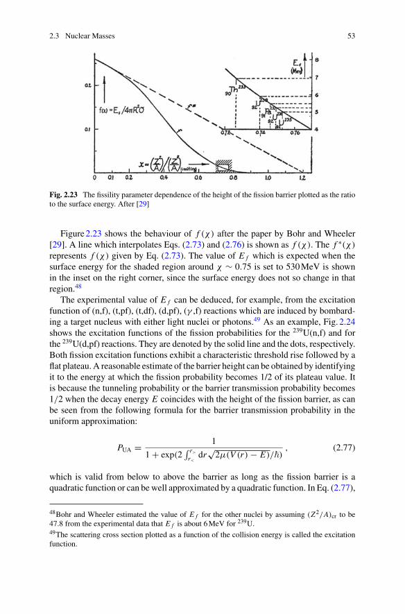
2.3 Nuclear Masses 53
Fig. 2.23 The fissility parameter dependence of the height of the fission barrier plotted as the ratioto the surface energy. After [29]
Figure2.23 shows the behaviour of f (χ) after the paper by Bohr and Wheeler[29]. A line which interpolates Eqs. (2.73) and (2.76) is shown as f (χ). The f ∗(χ)
represents f (χ) given by Eq. (2.73). The value of E f which is expected when thesurface energy for the shaded region around χ ∼ 0.75 is set to 530MeV is shownin the inset on the right corner, since the surface energy does not so change in thatregion.48
The experimental value of E f can be deduced, for example, from the excitationfunction of (n,f), (t,pf), (t,df), (d,pf), (γ ,f) reactions which are induced by bombard-ing a target nucleus with either light nuclei or photons.49 As an example, Fig. 2.24shows the excitation functions of the fission probabilities for the 239U(n,f) and forthe 239U(d,pf) reactions. They are denoted by the solid line and the dots, respectively.Both fission excitation functions exhibit a characteristic threshold rise followed by aflat plateau. A reasonable estimate of the barrier height can be obtained by identifyingit to the energy at which the fission probability becomes 1/2 of its plateau value. Itis because the tunneling probability or the barrier transmission probability becomes1/2 when the decay energy E coincides with the height of the fission barrier, as canbe seen from the following formula for the barrier transmission probability in theuniform approximation:
PUA = 1
1 + exp(2∫ r>
r<dr
√2μ(V (r) − E)/�)
, (2.77)
which is valid from below to above the barrier as long as the fission barrier is aquadratic function or can bewell approximated by a quadratic function. In Eq. (2.77),
48Bohr and Wheeler estimated the value of E f for the other nuclei by assuming (Z2/A)cr to be47.8 from the experimental data that E f is about 6MeV for 239U.49The scattering cross section plotted as a function of the collision energy is called the excitationfunction.
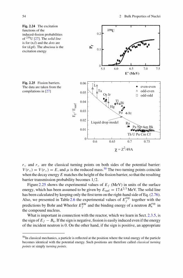
54 2 Bulk Properties of Nuclei
Fig. 2.24 The excitationfunctions of theinduced-fission probabilitiesof 239U [27]. The solid lineis for (n,f) and the dots arefor (d,pf). The abscissa is theexcitation energy
Fig. 2.25 Fission barriers.The data are taken from thecompilations in [27]
0
0.01
0.02
0.03
0.04
0.05
0.06
0.6 0.65 0.7 0.75
E f /
E sur
f
χ = Z2/49A
LuTa
Os Ir
HgTl Bi
Po At
Ra
Th U Pu Cm Cf
Pa Np Am BkLiquid drop model
even-evenodd-evenodd-odd
r< and r> are the classical turning points on both sides of the potential barrier:V (r<) = V (r>) = E , and μ is the reduced mass.50 The two turning points coincidewhen the decay energy E matches the height of the fission barrier, so that the resultingbarrier transmission probability becomes 1/2.
Figure2.25 shows the experimental values of E f (MeV) in units of the surfaceenergy, which has been assumed to be given by Esurf = 17A2/3MeV. The solid linehas been calculated by keeping only the first term on the right-hand side of Eq. (2.76).Also, we presented in Table2.6 the experimental values of Eexp.
f together with thepredictions by Bohr and Wheeler EBW
f and the binding energy of a neutron Bexp.n in
the compound nucleus.What is important in connection with the reactor, which we learn in Sect. 2.3.5, is
the sign of E f − Bn. If the sign is negative, fission is easily induced even if the energyof the incident neutron is 0. On the other hand, if the sign is positive, an appropriate
50In classical mechanics, a particle is reflected at the position where the total energy of the particlebecomes identical with the potential energy. Such positions are therefore called classical turningpoints or simply turning points.
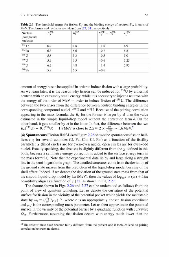
2.3 Nuclear Masses 55
Table 2.6 The threshold energy for fission E f and the binding energy of neutron Bn, in units ofMeV. The former and the latter are taken from [27, 31], respectively
Nucleus(compoundnucleus)
Eexp.f Bexp.
n Eexp.f − Bexp.
n EBWf
233Th 6.4 4.8 1.6 6.9232Pa 6.3 5.6 0.7 5.5235U 5.8 5.3 0.5 5.0236U 5.9 6.5 −0.6 5.25239U 6.2 4.8 1.4 5.95240Pu 5.9 6.5 −0.6
amount of energy has to be supplied in order to induce fissionwith a large probability.As we learn later, it is the reason why fission can be induced for 235U by a thermalneutron with an extremely small energy, while it is necessary to inject a neutron withthe energy of the order of MeV in order to induce fission of 238U. The differencebetween the two arises from the difference between neutron binding energies in thecorresponding compound nuclei, 236U and 239U. Because of the pairing correlationappearing in the mass formula, the Bn for the former is larger by Δ than the valueestimated in the simple liquid-drop model without the correction term δ. On theother hand, it gets smaller by Δ in the latter. In fact, the difference between the twoBn(
236U) − Bn(239U) = 1.7MeV is close to 2Δ ≈ 2 × 12√
238∼ 1.6MeV.51
(4) Spontaneous FissionHalf-Lives Figure2.26 shows the spontaneous fission half-lives t1/2 for several actinides (U, Pu, Cm, Cf, Fm) as a function of the fissilityparameter χ (filled circles are for even–even nuclei, open circles are for even–oddnuclei. Exactly speaking, the abscissa is slightly different from the χ defined in thisbook, because a symmetry energy correction is added to the surface energy term inthe mass formula). Note that the experimental data lie by and large along a straightline in the semi-logarithmic graph. The detailed structures come from the deviation ofthe ground state masses from the prediction of the liquid-drop model because of theshell effect. Indeed, if we denote the deviation of the ground state mass from that ofthe smooth liquid-drop model by δm (MeV), then the values of log10 t1/2 (yr) + 5δmbeautifully align as a function of χ [32] as shown in Fig. 2.27.
The feature shown in Figs. 2.26 and 2.27 can be understood as follows from thepoint of view of quantum tunneling. Let us denote the curvature of the potentialsurface for fission in the vicinity of the potential pocket which yields the metastablestate by ω0 ≡ ( ∂2V
∂r2 /μ f )1/2, where r is an appropriately chosen fission coordinate
and μ f is the corresponding mass parameter. Let us then approximate the potentialsurface in the vicinity of the potential barrier by a quadratic function with curvatureΩfb. Furthermore, assuming that fission occurs with energy much lower than the
51The reactor must have become fairly different from the present one if there existed no pairingcorrelation between nucleons.
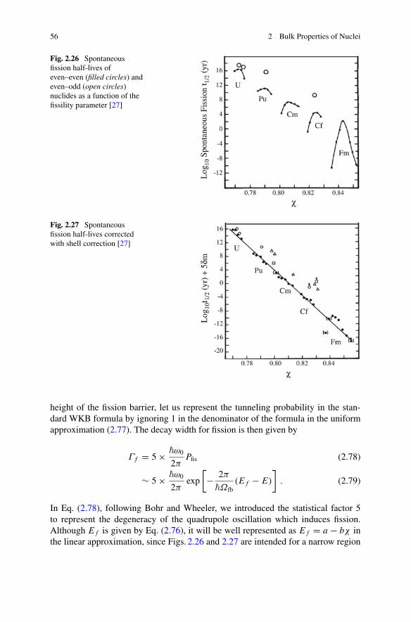
56 2 Bulk Properties of Nuclei
Fig. 2.26 Spontaneousfission half-lives ofeven–even (filled circles) andeven–odd (open circles)nuclides as a function of thefissility parameter [27]
Fig. 2.27 Spontaneousfission half-lives correctedwith shell correction [27]
height of the fission barrier, let us represent the tunneling probability in the stan-dard WKB formula by ignoring 1 in the denominator of the formula in the uniformapproximation (2.77). The decay width for fission is then given by
Γ f = 5 × �ω0
2πPfis (2.78)
∼ 5 × �ω0
2πexp
[− 2π
�Ωfb(E f − E)
]. (2.79)
In Eq. (2.78), following Bohr and Wheeler, we introduced the statistical factor 5to represent the degeneracy of the quadrupole oscillation which induces fission.Although E f is given by Eq. (2.76), it will be well represented as E f = a − bχ inthe linear approximation, since Figs. 2.26 and 2.27 are intended for a narrow region
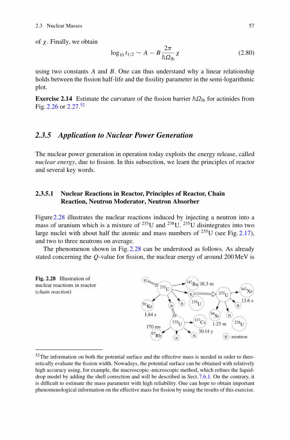
2.3 Nuclear Masses 57
of χ . Finally, we obtain
log10 t1/2 ∼ A − B2π
�Ωfbχ (2.80)
using two constants A and B. One can thus understand why a linear relationshipholds between the fission half-life and the fissility parameter in the semi-logarithmicplot.
Exercise 2.14 Estimate the curvature of the fission barrier �Ωfb for actinides fromFig. 2.26 or 2.27.52
2.3.5 Application to Nuclear Power Generation
The nuclear power generation in operation today exploits the energy release, callednuclear energy, due to fission. In this subsection, we learn the principles of reactorand several key words.
2.3.5.1 Nuclear Reactions in Reactor, Principles of Reactor, ChainReaction, Neutron Moderator, Neutron Absorber
Figure2.28 illustrates the nuclear reactions induced by injecting a neutron into amass of uranium which is a mixture of 235U and 238U. 235U disintegrates into twolarge nuclei with about half the atomic and mass numbers of 235U (see Fig. 2.17),and two to three neutrons on average.
The phenomenon shown in Fig. 2.28 can be understood as follows. As alreadystated concerning the Q-value for fission, the nuclear energy of around 200MeV is
Fig. 2.28 Illustration ofnuclear reactions in reactor(chain reaction)
52The information on both the potential surface and the effective mass is needed in order to theo-retically evaluate the fission width. Nowadays, the potential surface can be obtained with relativelyhigh accuracy using, for example, the macroscopic–microscopic method, which refines the liquid-drop model by adding the shell correction and will be described in Sect. 7.6.1. On the contrary, itis difficult to estimate the mass parameter with high reliability. One can hope to obtain importantphenomenological information on the effective mass for fission by using the results of this exercise.
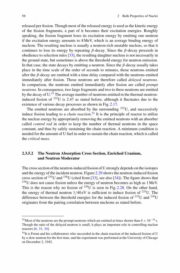
58 2 Bulk Properties of Nuclei
released per fission. Though most of the released energy is used as the kinetic energyof the fission fragments, a part of it becomes their excitation energies. Roughlyspeaking, the fission fragment loses its excitation energy by emitting one neutronif the excitation energy amounts to 8MeV, which is an average binding energy ofnucleon. The resulting nucleus is usually a neutron-rich unstable nucleus, so that itcontinues to lose its energy by repeating β-decay. Since the β-decay proceeds inobedience to selection rules [33], the resulting daughter nucleus is not necessarily inthe ground state, but sometimes is above the threshold energy for neutron emission.In that case, the state decays by emitting a neutron. Since the β-decay usually takesplace in the time scale of the order of seconds to minutes, those neutrons emittedafter the β-decay are emitted with a time delay compared with the neutrons emittedimmediately after fission. Those neutrons are therefore called delayed neutrons.In comparison, the neutrons emitted immediately after fission are called promptneutrons. In consequence, two large fragments and two to three neutrons are emittedby the decay of U.53 The average number of neutrons emitted in the thermal-neutron-induced fission of 235U is 2.47 as stated before, although it fluctuates due to theexistence of various decay processes as shown in Fig. 2.17.
The emitted neutrons are absorbed by the surrounding 235U, and successivelyinduce fission leading to a chain reaction.54 It is the principle of reactor to utilizethe nuclear energy by appropriately removing the emitted neutrons with an absorbercalled control rod in order to keep the number of thermal neutrons in the spaceconstant, and thus by safely sustaining the chain reaction. A minimum condition isneeded for the amount of U fuel in order to sustain the chain reaction, which is calledthe critical mass.
2.3.5.2 The Neutron Absorption Cross Section, Enriched Uranium,and Neutron Moderator
The cross section of the neutron-induced fission ofU strongly depends on the isotopesand the energy of the incident neutron. Figure2.29 shows the neutron-induced fissioncross section of 235U and 238U (cited from [33], see also [34]). The figure shows that238U does not cause fission unless the energy of neutron becomes as high as 1MeV.This is the reason why no fission of 238U is seen in Fig. 2.28. On the other hand,the energy of thermal neutron 1/40eV is sufficient to induce fission of 235U. Thedifference between the threshold energies for the induced fission of 235U and 238Uoriginates from the pairing correlation between nucleons as stated before.
53Most of the neutrons are the prompt neutrons which are emitted at times shorter than 4 × 10⁻¹⁴ s.Though the ratio of the delayed neutron is small, it plays an important role in controlling nuclearreactors [6, 33, 34].54It is Fermi and his collaborators who succeeded in the chain reaction of the induced fission of Uby a slow neutron for the first time, and the experiment was performed at the University of Chicagoon December 2, 1942.
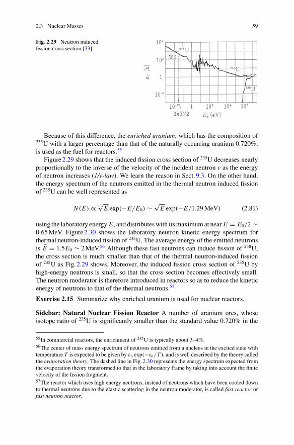
2.3 Nuclear Masses 59
Fig. 2.29 Neutron inducedfission cross section [33]
Because of this difference, the enriched uranium, which has the composition of235U with a larger percentage than that of the naturally occurring uranium 0.720%,is used as the fuel for reactors.55
Figure2.29 shows that the induced fission cross section of 235U decreases nearlyproportionally to the inverse of the velocity of the incident neutron v as the energyof neutron increases (1/v-law). We learn the reason in Sect. 9.3. On the other hand,the energy spectrum of the neutrons emitted in the thermal neutron induced fissionof 235U can be well represented as
N (E) ∝ √E exp(−E/E0) ∼ √
E exp(−E/1.29MeV) (2.81)
using the laboratory energy E , and distributeswith itsmaximum at near E = E0/2 ∼0.65MeV. Figure2.30 shows the laboratory neutron kinetic energy spectrum forthermal neutron-induced fission of 235U. The average energy of the emitted neutronsis E = 1.5E0 ∼ 2MeV.56 Although these fast neutrons can induce fission of 238U,the cross section is much smaller than that of the thermal neutron-induced fissionof 235U as Fig. 2.29 shows. Moreover, the induced fission cross section of 235U byhigh-energy neutrons is small, so that the cross section becomes effectively small.The neutron moderator is therefore introduced in reactors so as to reduce the kineticenergy of neutrons to that of the thermal neutrons.57
Exercise 2.15 Summarize why enriched uranium is used for nuclear reactors.
Sidebar: Natural Nuclear Fission Reactor A number of uranium ores, whoseisotope ratio of 235U is significantly smaller than the standard value 0.720% in the
55In commercial reactors, the enrichment of 235U is typically about 3–4%.56The center of mass energy spectrum of neutrons emitted from a nucleus in the excited state withtemperature T is expected to be given by εn exp(−εn/T ), and is well described by the theory calledthe evaporation theory. The dashed line in Fig. 2.30 represents the energy spectrum expected fromthe evaporation theory transformed to that in the laboratory frame by taking into account the finitevelocity of the fission fragment.57The reactor which uses high energy neutrons, instead of neutrons which have been cooled downto thermal neutrons due to the elastic scattering in the neutron moderator, is called fast reactor orfast neutron reactor.
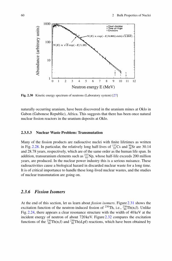
60 2 Bulk Properties of Nuclei
Fig. 2.30 Kinetic energy spectrum of neutrons (Laboratory system) [27]
naturally occurring uranium, have been discovered in the uranium mines at Oklo inGabon (Gabonese Republic), Africa. This suggests that there has been once naturalnuclear fission reactors in the uranium deposits at Oklo.
2.3.5.3 Nuclear Waste Problem: Transmutation
Many of the fission products are radioactive nuclei with finite lifetimes as writtenin Fig. 2.28. In particular, the relatively long half-lives of 137
55Cs and9038Sr are 30.14
and 28.78 years, respectively, which are of the same order as the human life span. Inaddition, transuranium elements such as 237
93Np, whose half-life exceeds 200 millionyears, are produced. In the nuclear power industry this is a serious nuisance. Theseradioactivities cause a biological hazard in discarded nuclear waste for a long time.It is of critical importance to handle these long-lived nuclear wastes, and the studiesof nuclear transmutation are going on.
2.3.6 Fission Isomers
At the end of this section, let us learn about fission isomers. Figure2.31 shows theexcitation function of the neutron-induced fission of 230Th, i.e., 23090 Th(n,f). UnlikeFig. 2.24, there appears a clear resonance structure with the width of 40keV at theincident energy of neutron of about 720keV. Figure2.32 compares the excitationfunctions of the 230
90 Th(n,f) and23090 Th(d,pf) reactions, which have been obtained by
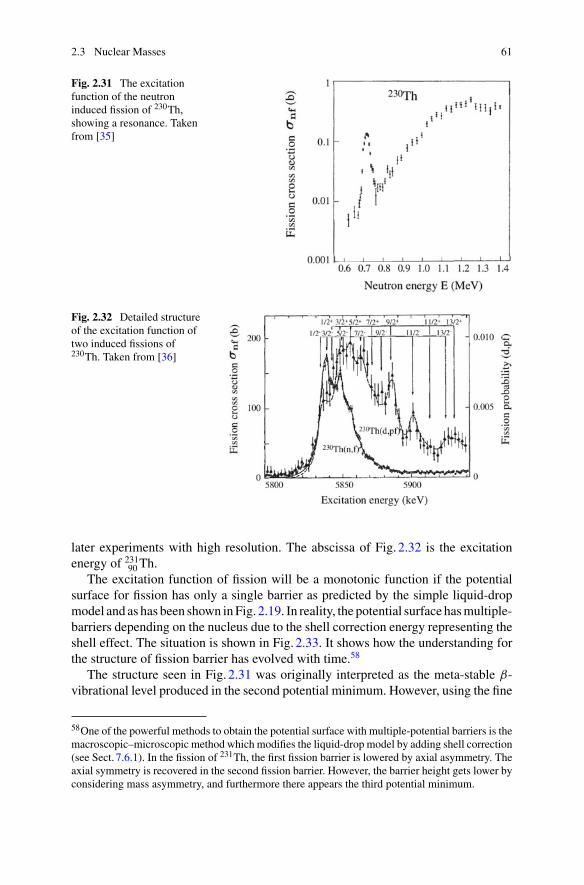
2.3 Nuclear Masses 61
Fig. 2.31 The excitationfunction of the neutroninduced fission of 230Th,showing a resonance. Takenfrom [35]
Fig. 2.32 Detailed structureof the excitation function oftwo induced fissions of230Th. Taken from [36]
later experiments with high resolution. The abscissa of Fig. 2.32 is the excitationenergy of 231
90 Th.The excitation function of fission will be a monotonic function if the potential
surface for fission has only a single barrier as predicted by the simple liquid-dropmodel and as has been shown inFig. 2.19. In reality, the potential surface hasmultiple-barriers depending on the nucleus due to the shell correction energy representing theshell effect. The situation is shown in Fig. 2.33. It shows how the understanding forthe structure of fission barrier has evolved with time.58
The structure seen in Fig. 2.31 was originally interpreted as the meta-stable β-vibrational level produced in the second potential minimum. However, using the fine
58One of the powerful methods to obtain the potential surface with multiple-potential barriers is themacroscopic–microscopic method which modifies the liquid-drop model by adding shell correction(see Sect. 7.6.1). In the fission of 231Th, the first fission barrier is lowered by axial asymmetry. Theaxial symmetry is recovered in the second fission barrier. However, the barrier height gets lower byconsidering mass asymmetry, and furthermore there appears the third potential minimum.
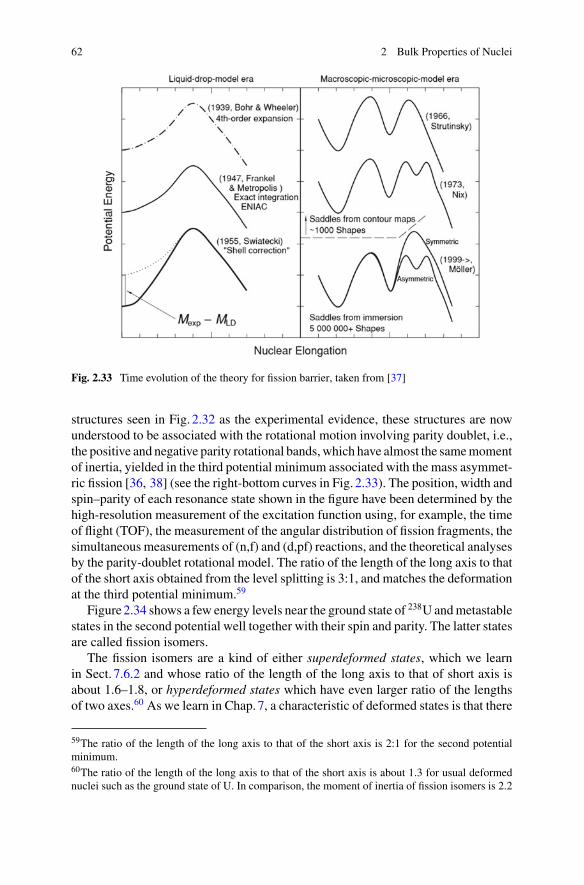
62 2 Bulk Properties of Nuclei
Fig. 2.33 Time evolution of the theory for fission barrier, taken from [37]
structures seen in Fig. 2.32 as the experimental evidence, these structures are nowunderstood to be associated with the rotational motion involving parity doublet, i.e.,the positive and negative parity rotational bands,which have almost the samemomentof inertia, yielded in the third potential minimum associated with the mass asymmet-ric fission [36, 38] (see the right-bottom curves in Fig. 2.33). The position, width andspin–parity of each resonance state shown in the figure have been determined by thehigh-resolution measurement of the excitation function using, for example, the timeof flight (TOF), the measurement of the angular distribution of fission fragments, thesimultaneous measurements of (n,f) and (d,pf) reactions, and the theoretical analysesby the parity-doublet rotational model. The ratio of the length of the long axis to thatof the short axis obtained from the level splitting is 3:1, and matches the deformationat the third potential minimum.59
Figure2.34 shows a few energy levels near the ground state of 238U andmetastablestates in the second potential well together with their spin and parity. The latter statesare called fission isomers.
The fission isomers are a kind of either superdeformed states, which we learnin Sect. 7.6.2 and whose ratio of the length of the long axis to that of short axis isabout 1.6–1.8, or hyperdeformed states which have even larger ratio of the lengthsof two axes.60 As we learn in Chap.7, a characteristic of deformed states is that there
59The ratio of the length of the long axis to that of the short axis is 2:1 for the second potentialminimum.60The ratio of the length of the long axis to that of the short axis is about 1.3 for usual deformednuclei such as the ground state of U. In comparison, the moment of inertia of fission isomers is 2.2
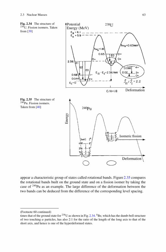
2.3 Nuclear Masses 63
Fig. 2.34 The structure of238U. Fission isomers. Takenfrom [39]
Fig. 2.35 The structure of240Pu. Fission isomers.Taken from [40]
appear a characteristic group of states called rotational bands. Figure2.35 comparesthe rotational bands built on the ground state and on a fission isomer by taking thecase of 240Pu as an example. The large difference of the deformation between thetwo bands can be deduced from the difference of the corresponding level spacing.
(Footnote 60 continued)times that of the ground state for 238U as shown in Fig. 2.34. 8Be, which has the dumb-bell structureof two touching α particles, has also 2:1 for the ratio of the length of the long axis to that of theshort axis, and hence is one of the hyperdeformed states.
64 2 Bulk Properties of Nuclei
References
1. E. Segré, From X-Rays to Quarks: Modern Physicists and Their Discoveries (W. H. Freemanand Company, San Francisco, 1980)
2. M. Nogami, Nuclear Physics, Japanese edn. (Shoukabou, Tokyo, 1973)3. T. de Forest Jr., J.D. Walecka, Adv. Phys. 15, 1 (1966)4. B. Hahn, D.G. Ravenhall, R. Hofstadter, Phys. Rev. 101, 1131 (1956)5. A. Tamii et al., Phys. Rev. Lett. 107, 062502 (2011)6. W.N. Cottingham, D.A. Greenwood, An Introduction to Nuclear Physics, 2nd edn. (Cambridge
University Press, Cambridge, 2001)7. R. Hofstadter, F. Bumiller, M.R. Yearian, Rev. Mod. Phys. 30, 482 (1958)8. N. Takigawa, M. Ueda, M. Kuratani, H. Sagawa, Phys. Lett. B 288, 244 (1992)9. J.S. Al-Khalili, J.A. Tostevin, Phys. Rev. Lett. 76, 3903 (1996)10. B. Abu-Ibrahim, Y. Suzuki, Phys. Rev. C 61, 051601 (2000)11. J. Kasagi, H. Yuki, T. Baba, T. Noda, T. Ohtsuki, A.G. Lipson, J. Phys. Soc. Jpn. 71, 2881
(2002)12. Y. Kato, N. Takigawa, Phys. Rev. C 76, 014615 (2007). And references therein13. G. Audi, A.H. Wapstra, C. Thibault, Nucl. Phys. A 729, 337 (2003)14. R. Shurtleff, E. Derringh, Am. J. Phys. 57, 552 (1989)15. T. Arima, Master thesis, Tohoku University16. W.-M. Yao et al. (Particle Data Group), J. Phys. G 33, 1 (2006)17. L. Alvarez et al., Phys. Rev. 105, 1127 (1957)18. S.E. Jones, Nature 321, 127 (1986)19. K. Ikeda, N. Takigawa, H. Horiuchi, Prog. Theor. Phys. Suppl. E68, 464 (1968)20. K. Ikeda, T. Marumori, R. Tamagaki, H. Tanaka, J. Hiura, H. Horiuchi, Y. Suzuki, F. Nemoto,
H. Bando, Y. Abe, N. Takigawa, M. Kamimura, K. Takada, Y. Akaishi, S. Nagata, Prog. Theor.Phys. Suppl. 52 (1972); K. Ikeda, R. Tamagaki, S. Saito, H. Horiuchi, A. Tohsaki-Suzuki, M.Kamimura, Prog. Theor. Phys. Suppl. 62 (1977)
21. H. Horiuchi, K. Ikeda, K. Kato, Prog. Theor. Phys. Suppl. 192, 1 (2012)22. C.M. Lederer, V. Shirley, Table of Isotopes, 7th edn. (Wiley, New York, 1978)23. N. Takigawa, A. Arima, Nucl. Phys. A 168, 593 (1971)24. P. Möller, J.R. Nix, W.D. Myers, W.J. Swiatecki, At Data Nucl. Tables 59, 185 (1995); P.
Möller, J.R. Nix, Nucl. Phys. A 536, 20 (1992); H. Koura, M. Uno, T. Tachibana, M. Yamada,Nucl. Phys. A 674, 47 (2000); H. Koura, T. Tachibana, M. Uno, M. Yamada. Prog. Theor. Phys.113, 305 (2005)
25. S. Yusa, private communication26. K.F. Flynn, L.E. Glendenin, ANL-7749 (1970); cited in [27]27. R. Vandenbosch, J.R. Huizenga, Nuclear Fission (Academic Press, New York, 1973)28. O. Hahn, F. Strassmann, Naturwiss. 27, 11 (1939)29. N. Bohr, J.A. Wheeler, Phys. Rev. 56, 426 (1939)30. F. Ivanyuk, K. Pomorski, Phys. Rev. C 79, 054327 (2009); Int. J. Mod. Phys. E 19, 514 (2010)31. A.H. Wapstra, G. Audi, Nucl. Phys. A 432, 1 (1985)32. W.J. Swiatecki, Phys. Rev. 100, 937 (1955)33. K. Yagi, Nuclear Physics, Japanese edn. (Asakura, Tokyo, 1971)34. W.S.C. Williams, Nuclear and Particle Physics (Clarendon press, Oxford, 1991)35. G.D. James, J.E. Lynn, L.G. Earwaker, Nucl. Phys. A 189, 225 (1972)36. J. Blons, Nucl. Phys. A 502, 121c (1989)37. P. Möller, A.J. Sierk, T. Ichikawa, A. Iwamoto, R. Bengtsson, H. Uhrenholt, S. Åberg, Phys.
Rev. C 79, 064304 (2009)38. P. Möller, J.R. Nix, in Proceedings of the Third IAEA Symposium on the Physics and Chemistry
of Fission, Rochester, 1973, Vol. I (International Atomic Energy Agency, Vienna, 1974), p. 10339. R. Vandenbosch, Nucl. Phys. A 502, 1c (1989)40. V. Metag, D. Habs, H.J. Specht, Phys. Rep. 65, 1 (1980); The original paper is H.J. Specht, J.
Weber, E. Konecny, D. Heunemann. Phys. Lett. B 41, 43 (1972)
Chapter 3The Nuclear Force and Two-Body Systems
Abstract The strong interaction between nucleons which is called the nuclear forceplays the central role in nuclear physics. Compared with the Coulomb interactionbetween two charged particles, which plays the exclusive role in condensed matterphysics, the nuclear force is fairly complicated reflecting the fact that nucleons arecomposite particles and have spin and isospin degrees of freedom. There are severaldifferent approaches to uncover nuclear force. The one is to consider themost generalpossibility under the constraints from the consideration of symmetry or transforma-tion invariance. The other is a phenomenological approach. The meson theory is alsoan attractive historical approach, which is often combined with phenomenologicalapproaches. Recently, approaches based on QCD are also introduced. A difficultyof nuclear force is that the effective force inside nucleus is fairly different from thebare interaction between two nucleons in free space. In this chapter we overview thebasic properties and the current understanding of the nuclear force.
3.1 The Fundamentals of Nuclear Force
3.1.1 The Range of Forces—A Simple Estimateby the Uncertainty Principle
The four forces in nature, i.e., the gravitational force, the electromagnetic force, theweak interaction and the strong interaction, can be thought to originate from exchang-ing gauge particles, i.e., graviton, photon, weak bosons (W± and Z0 particles) andmesons (or gluons at the more fundamental level of the quantum chromodynamics(QCD)), which mediate each force, between two particles. Following this idea, onecan relate the range of each force to the mass of the corresponding gauge particlesusing the uncertainty principle.
If we denote the mass of a gauge particle by m, then the uncertainty of the energyassociated with the propagation of the gauge particle is ΔE ∼ mc2. Hence, thecorrespondinguncertainty of time isΔt ∼ �/ΔE ∼ �/mc2.Assuming that the gaugeparticle moves with the light velocity during that time interval, the range of the forced can be estimated to be
© Springer Japan 2017N. Takigawa and K. Washiyama, Fundamentals of Nuclear Physics,DOI 10.1007/978-4-431-55378-6_3
65
66 3 The Nuclear Force and Two-Body Systems
d ∼ c × Δt ∼ �
mc, (3.1)
and coincides with the Compton wavelength of the gauge particle. As is well known,the electromagnetic force reaches infinite distance, because the mass of photon iszero. On the other hand, the range of the weak interaction is very short, since themasses of W± and Z0 particles are large. If we assume that the strong interaction ismediated by exchanging mesons as we learn later in the meson theory, the range ofthe force which originates from the exchange of the lightest meson, i.e., π -mesons,can be estimated to be about 1.4 fm by using that the rest energy of the π -mesons isabout 140MeV. Incidentally, although the graviton has not yet been discovered, itsmass is expected to be zero, because the gravitational force has an infinite range likethe electromagnetic force.
3.1.2 The Radial Dependence
Though we made a rough estimate of the range of forces using the uncertaintyprinciple in the previous section, the strength of the nuclear force acting betweentwo particles varies as a function of the distance between them similarly to that thestrength of the Coulomb interaction gets weaker in inverse proportion to the squareof the distance r between the two charged particles as their distance increases.
Corresponding to the fact that the strength of the Coulomb force is proportionalto 1/r2, the Coulomb potential is given by VC(r) = Q1Q2e2/r , where Q1e and Q2eare the electric charges of the two charged particles. This formula can be derived bythinking that one of the chargedparticles produces an electric field through interactionwith the electromagnetic field, and then exerts a force on the other charged particlevia the electric field. The equation which determines the electric field in this case isknown as the D’Alembert equation.
The same idea can be applied to the strong interaction. If we denote the field ofthe strong interaction by φ(r, t), then the equation called Klein–Gordon equation,which is a generalization of the D’Alembert equation for the electric force, is givenby [
∇2 − 1
c2∂2
∂t2−
(mc
�
)2]
φ(r, t) = −4πρ(r, t) , (3.2)
wherem is themass of the gauge particle. It is themass of ameson in themeson theoryfor the nuclear force. There appears on the left-hand side the Compton wavelengthof the gauge particle because of the finiteness of the mass of the gauge particle. Theρ(r, t) appearing on the right-hand side represents the density at the spatial positionr at time t of the charged particles which create the electric force in the D’Alembertequation for the Coulomb potential. It is the density of hadrons such as nucleons,which are the sources of mesons or gluons, in the case of the strong interaction.
In the static limit to ignore the time variation, the solution of Eq. (3.2) is given by
3.1 The Fundamentals of Nuclear Force 67
φ(r, t) ≈∫
ρ(r′, t)e−mc|r−r′|/�
|r − r′| dr′ . (3.3)
Exercise 3.1 Derive Eq. (3.3) by the following two methods 1 and 2.
1. The method of Fourier transformation
a. Show that the Fourier transformation of φ(r) is given by
φ(k) = 4π
k2 + (mc/�)2ρ(k, t) . (3.4)
b. Derive Eq. (3.3) by making the inverse Fourier transformation of φ(k).
2. The Green function methodDefine the Green function in the static case by
[∇2 −
(mc
�
)2]
G N (r − r′) = −4πδ(r − r′) , (3.5)
and then show that it becomes
G N (r − r′) = e−mc|r−r′|/�
|r − r′| . (3.6)
Exercise 3.2 Prove the following equation.
∇2 1
|r − r′| = −4πδ(r − r′) . (3.7)
The nuclear potential φN (r) can be obtained by letting ρ(r′) = ρ0δ(r′) in theintegral on the right-hand side of Eq. (3.3) in the limit of ignoring the size of theparticle such as a nucleon which is the source of the force. Here, we took the positionof the hadronwhich is the source of the force as the origin of the spatial coordinate.Wecan see that the distance dependence changes from the 1/r law for the electric forceto e−μr/r with μ = mc/�. This functional form including the exponential dampingfactor is called the Yukawa type, and the strength of the nuclear force becomese−1 ≈ 1/2.7 in the distance of 1/μ. This distance corresponds to the range of theforce which we obtained in the previous section and coincides with the Comptonwavelength of the gauge particle.
3.1.3 The State Dependence of Nuclear Force
In the following, we discuss the interaction between two nucleons, called nuclearforce, among the strong interactions. Since each nucleon has the spin degree of
68 3 The Nuclear Force and Two-Body Systems
freedom, and also the degree of freedom in the isospin space, which has been touchedin Sect. 1.2, in addition to that in the usual space, the nuclear force is much morecomplex than the Coulomb force, and causes a great variety of phenomena. In thissection, we learn the classification of the states of two-nucleon systems, the exchangeoperators and the projection operators in preparation for studying more details aboutthe nuclear force.
3.1.3.1 The Classification of the States of Two-Nucleon Systems
The wave function of two-nucleon systems ψ can be expressed as the product of thewave functions in the usual space, the spin space and the isospin space as
ψ(x1, x2) = ϕ(r)ζ(s1, s2)η(t1, t2) (3.8)
if there is no interaction between the coordinates in the usual and spin spaces suchas the spin–orbit interaction which we will learn in Sect. 3.2.2. The s and t are thez-components of the coordinates in the spin and isospin spaces, the lower indices1 and 2 refer to the first and the second nucleons, r ≡ r1 − r2 is the coordinate for therelative motion, r1 and r2 the spatial coordinates of the first and the second nucleons,respectively. Also, x is used to represent the coordinates in the usual, spin and isospinspaces altogether simultaneously, i.e., x = (r, s, t).
If one uses the simultaneous eigenstates of the square S2 of the total spinS ≡ s1 + s2 and its z-component Sz , |S, Sz〉, then the wave function in the spin spaceζ is one of the following states,
|1, 1〉S = α1α2 , (3.9)
|1, 0〉S = 1√2[α1β2 + β1α2] , (3.10)
|1,−1〉S = β1β2 , (3.11)
|0, 0〉S = 1√2[α1β2 − β1α2] . (3.12)
We ignored the coordinates on the left-hand side, but used the indexS to explicitlyindicate that it is the wave function in the spin space. On the right-hand side, weexpressed the coordinates s1 and s2 simply with the lower index 1 and 2. The α
and β represent the spin-up and spin-down states, | 12 12 〉 and | 12 − 1
2 〉, respectively.The states with S = 1 and S = 0 are symmetric and antisymmetric concerning thetwo nucleons, respectively, and does not change and changes the sign when the twonucleons are interchanged. The former and the latter are called the spin-triplet andthe spin-singlet states, respectively.
Similarly, the wave function in the isospin space η can be expressed using the fol-lowing simultaneous eigenstates of the square of the total isospin and the magnitudeof its z-component,
3.1 The Fundamentals of Nuclear Force 69
|1, 1〉I = n1n2 , (3.13)
|1, 0〉I = 1√2[n1p2 + p1n2] , (3.14)
|1,−1〉I = p1p2 , (3.15)
|0, 0〉I = 1√2[n1p2 − p1n2] , (3.16)
and each state can be classified into either isospin-triplet or isospin-singlet states.The lower index I means isospin space. As defined in Eq. (1.3), n and p representneutron (isospin-up) and proton (isospin-down) states, respectively.
On the other hand, the wave function for the relative motion can also be classifiedinto either symmetric or antisymmetric states with respect to the exchange of twonucleons. Since the exchange of two particles corresponds to the parity transforma-tion (or the parity inversion) of the coordinate of the relative motion r, the formerstate is called E-state in the sense of even, while the latter O-state in the sense ofodd state. For example, if the wave function ϕ(r) is given by ϕ(r) = R�(r)Y�m(θ, φ)
by using the spherical harmonics Y�m , then the states with an even number for theorbital angular momentum � such as the s-wave are E-states, while those with odd-�values such as the p-wave are O-states.
Let us now represent the state for two-nucleon systems as 2T +1 2S+1E or 2T +1 2S+1Owhen the total spin and the total isospin are S and T . The symbols E and O representthe symmetry property, i.e., the even–odd property, of the wave function of therelative motion. Since nucleons are fermions, the wave function of two-nucleonsystems has to change sign for the simultaneous coordinate interchange in the wholespace. Namely, ψ(x2, x1) = −ψ(x1, x2). Hence only the following four states, 13E,31E, 11O, 33O, are allowed for two-nucleon systems. For example, 13E is called singlettriplet even state. A characteristic of the nuclear force is that it significantly differsin these four states.
3.1.3.2 The Exchange Operators
(1) The Spin-ExchangeOperatorVarious exchanges take place when two nucleonsinteract. For example, when a proton in the spin-up state collides with another protonin the spin-down state, the orientation of the spin is interchanged between themwith acertain probability (spin exchange). This happens because the nuclear force containsterms which are proportional to the inner product σ 1 · σ 2 of the spins of the twonucleons. We can rewrite the inner product as
σ 1 · σ 2 = 1
2(σ1+σ2− + σ1−σ2+) + σ1z σ2z (3.17)
by using the raising and lowering operators of the spin. The spin exchange processesare caused by the first and the second terms on the right-hand side.
70 3 The Nuclear Force and Two-Body Systems
It is convenient to introduce the following operator in order to describe the spinexchange effect,
Pσ = 1
2(1 + σ 1 · σ 2) . (3.18)
One can easily show that Pσ |1M〉S = |1M〉S (M = 1, 0,−1) and Pσ |00〉S =−|00〉S by operating Pσ on the spin-triplet and spin-singlet states. Since thespin-triplet and spin-singlet states are symmetric and antisymmetric regarding theexchange of the spins of two nucleons, this means that Pσ has the same functionas the exchange of the spins of the two nucleons. For this reason, Pσ is called thespin-exchange operator, alternatively the Bartlett operator.
(2) TheCharge-ExchangeOperator The exchange of isospin can also occur in two-nucleon systems. For example, a proton and a neutron are interchanged when theycollide (charge exchange). In order to describe this phenomenon, it is convenient tointroduce the following charge-exchange operator, which is also called the isospin-exchange operator or the Heisenberg operator, by using the isospin operator τ ofeach nucleon,
Pτ = 1
2(1 + τ 1 · τ 2) . (3.19)
(3) The space-Exchange Operator (Majorana Operator) One can also considerthe operator which interchanges the coordinates of two nucleons in the usual space.It is denoted by PM,
PMϕ(r) = ϕ(−r) . (3.20)
Since the wave function for two-nucleon systems has to be antisymmetric in wholespace,
PMPτ Pσψ = −ψ . (3.21)
Hence,PMPτ Pσ = −1 . (3.22)
One can therefore writePM = −Pτ Pσ . (3.23)
3.1.3.3 The Projection Operators
As we see later, the nuclear force strongly depends on the states of two nucleonsthrough the σ 1 · σ 2 and τ 1 · τ 2 terms in the nuclear force.
One often uses the projection operators defined by
Πst ≡ 1
4(3 + σ 1 · σ 2) , Πss ≡ 1
4(1 − σ 1 · σ 2) , (3.24)
Πi t ≡ 1
4(3 + τ 1 · τ 2) , Πis ≡ 1
4(1 − τ 1 · τ 2) , (3.25)
3.1 The Fundamentals of Nuclear Force 71
in order to explicitly show the state dependence of the nuclear force. The indicesst, ss, i t and is represent to project on the spin-triplet states, spin-singlet state,isospin-triplet states and isospin-singlet state, respectively.
Exercise 3.3 Show that Πst satisfies the following conditions which are requiredfor the projection operator on the spin-triplet states.
Π2st = Πst , ΠstΠss = 0 , Πst |1M〉S = |1M〉S , Πst |00〉S = 0 . (3.26)
3.2 The General Structure of Nuclear Force
One of the methods to construct nuclear force or nuclear potential is to take intoaccount various conservation laws suggested by fundamental experiments and toconsider the most general structure of the nuclear potential under those constraints.Each conservation law is related to the invariance or symmetry under an associatedtransformation. For nuclear force, one can first list up that
• the potential is a scalar quantity,• it is invariant under space reflection, i.e., Parity invariant,• it is time reversal invariant
as the basic properties. Furthermore, the proton–proton and proton–neutron scatter-ings at low energies suggest that the nuclear force is the same for the three states ofisospin triplets to a high accuracy. This is called the charge independence and impliesthat the nuclear force is a function of the inner product of the isospins of two nucleonsτ 1 · τ 2. On the other hand, the way of thinking that the force between two neutronsand that between two protons are the same is called the charge symmetry. The chargesymmetry and the charge independence are suggested also from the facts that theenergy levels of mirror nuclei, e.g., 157N8 and 15
8O7, very much resemble except forthe energy shift due to the Coulomb energy, and that there appear correspondingenergy levels among isobars such as 14
8O6, 147N7 and 146C8.1
In this section, we give the general form of the nuclear potential based on theconsiderations of the invariance or the symmetry.
3.2.1 Static Potentials (Velocity-Independent Potentials)
Let us first consider the potentials, called static potentials, which do not depend onthe velocity of the relative motion between the nucleons.
1A group of energy levels which have the same Jπ but differ in the z-component of the isospin forman isobaric multiplet. For example, there exist many isobaric triplets for 148 O6, 147 N7, and 14
6 C8.
72 3 The Nuclear Force and Two-Body Systems
3.2.1.1 Central Potentials
The static potentials can be classified into the central potentials, which depend onlyon the distance r between the nucleons, and the noncentral potentials, which dependon the angle of the relative coordinate r. The most general central static potentialcan be written as
VC = V0(r) + (σ 1 · σ 2)Vσ (r) + (τ 1 · τ 2)Vτ (r) + (σ 1 · σ 2)(τ 1 · τ 2)Vστ (r)
(3.27)
by considering the symmetry and invariance conditionsmentioned at the beginning ofthis section. The strength and the functional form of V0(r), Vσ (r), Vτ (r) and Vστ (r)
cannot be determined by the consideration of symmetry alone. Equation (3.27) canbe rewritten as
VC = VW(r) + VM(r)PM + VB(r)Pσ + VH(r)Pτ , (3.28)
where the indices W, M, B and H stand for Wigner, Majorana, Bartlett, andHeisenberg, respectively, or
VC = Vst (r)Πst + Vts(r)Πts + Vtt (r)Πt t + Vss(r)Πss (3.29)
by using the exchange and projection operators. Here, Πst is the projection oper-ator on the isospin-singlet, spin-triplet states and is given by Πst ≡ Πis × Πst .Πts, Πt t , Πss are defined in a similar way. The radial functions in the different rep-resentations are transformed as
VW = V0 − Vσ − Vτ + Vστ ,
VM = −4Vστ ,
VB = 2Vσ − 2Vστ ,
VH = 2Vτ − 2Vστ , (3.30)
and
Vts = VW + VM − VB + VH = V0 − 3Vσ + Vτ − 3Vστ ,
Vst = VW + VM + VB − VH = V0 + Vσ − 3Vτ − 3Vστ ,
Vss = VW − VM − VB − VH = V0 − 3Vσ − 3Vτ + 9Vστ ,
Vtt = VW − VM + VB + VH = V0 + Vσ + Vτ + Vστ . (3.31)
Exercise 3.4 Show the relationships (3.30) and (3.31).
3.2 The General Structure of Nuclear Force 73
3.2.1.2 Noncentral Potentials
One can make an operator which satisfies the invariant conditions for nuclear forcein the following way,
S12 = 3(r · σ 1)(r · σ 2)
r2− σ 1 · σ 2 , (3.32)
by using the relative coordinate r between the nucleons and the spin of each nucleon.Equation (3.32) can be represented in the form,
S12 = (24π)1/2[[σ (1)1 × σ
(1)2 ](λ=2) × Y2(r)](0)0 , (3.33)
by using the notation of the tensor product. The S12 is therefore called the tensoroperator. Using the total spin of two-nucleon system,
S = 1
2(s1 + s2) , (3.34)
S12 can be rewritten also as
S12 = 2
[3(S · r)2
r2− S
2
]. (3.35)
Equation (3.35) shows that S12 has a finite value only when it is operated on thespin-triplet states. Hence one can represent the noncentral potential as
VT = [V even
T (r)Π(T = 0, Leven) + V oddT (r)Π(T = 1, Lodd)
]S12 , (3.36)
where Π(T = 0, Leven) and Π(T = 1, Lodd) are the projection operators on theisospin 0, even parity states and on the isospin 1, odd parity states, respectively.This force is called the tensor force. As the form of Eq. (3.32) shows, the tensorforce resembles the force acting between two magnetic dipoles. We learn later thatthe tensor force is responsible for binding the deuteron among various two-nucleonsystems, and plays a vital role in the existence of nuclei, e.g., in locating the stablenuclei along the diagonal line in the nuclear chart.
Exercise 3.5 Show Eqs. (3.33) and (3.35).
3.2.2 Velocity-Dependent Potentials
A representative of the velocity-dependent potentials is the spin–orbit interaction,whose corresponding potential is given by
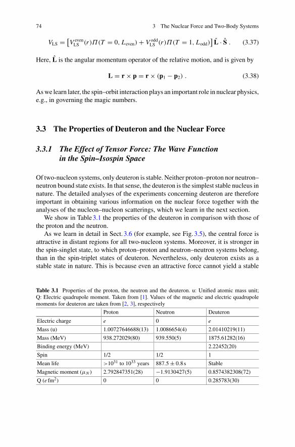
74 3 The Nuclear Force and Two-Body Systems
VLS = [V evenLS (r)Π(T = 0, Leven) + V odd
LS (r)Π(T = 1, Lodd)]L · S . (3.37)
Here, L is the angular momentum operator of the relative motion, and is given by
L = r × p = r × (p1 − p2) . (3.38)
Aswe learn later, the spin–orbit interaction plays an important role in nuclear physics,e.g., in governing the magic numbers.
3.3 The Properties of Deuteron and the Nuclear Force
3.3.1 The Effect of Tensor Force: The Wave Functionin the Spin–Isospin Space
Of two-nucleon systems, only deuteron is stable. Neither proton–proton nor neutron–neutron bound state exists. In that sense, the deuteron is the simplest stable nucleus innature. The detailed analyses of the experiments concerning deuteron are thereforeimportant in obtaining various information on the nuclear force together with theanalyses of the nucleon–nucleon scatterings, which we learn in the next section.
We show in Table3.1 the properties of the deuteron in comparison with those ofthe proton and the neutron.
As we learn in detail in Sect. 3.6 (for example, see Fig. 3.5), the central force isattractive in distant regions for all two-nucleon systems. Moreover, it is stronger inthe spin-singlet state, to which proton–proton and neutron–neutron systems belong,than in the spin-triplet states of deuteron. Nevertheless, only deuteron exists as astable state in nature. This is because even an attractive force cannot yield a stable
Table 3.1 Properties of the proton, the neutron and the deuteron. u: Unified atomic mass unit;Q: Electric quadrupole moment. Taken from [1]. Values of the magnetic and electric quadrupolemoments for deuteron are taken from [2, 3], respectively
Proton Neutron Deuteron
Electric charge e 0 e
Mass (u) 1.00727646688(13) 1.0086654(4) 2.01410219(11)
Mass (MeV) 938.272029(80) 939.550(5) 1875.61282(16)
Binding energy (MeV) 2.22452(20)
Spin 1/2 1/2 1
Mean life >1031 to 1033 years 887.5 ± 0.8s Stable
Magnetic moment (μN ) 2.792847351(28) −1.9130427(5) 0.8574382308(72)
Q (e fm2) 0 0 0.285783(30)
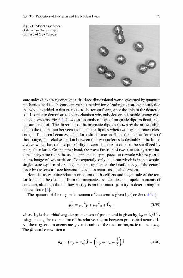
3.3 The Properties of Deuteron and the Nuclear Force 75
Fig. 3.1 Model experimentof the tensor force. Toyscourtesy of Gyo Takeda
state unless it is strong enough in the three dimensional world governed by quantummechanics, and also because an extra attractive force leading to a stronger attractionas a whole is added to deuteron due to the tensor force, since the spin of the deuteronis 1. In order to demonstrate the mechanism why only deuteron is stable among two-nucleon systems, Fig. 3.1 shows an assembly of toys of magnetic dipoles floating onthe surface of oil. The directions of the magnetic dipoles shown by the arrows aligndue to the interaction between the magnetic dipoles when two toys approach closeenough. Deuteron becomes stable for a similar reason. Since the nuclear force is ofshort range, the relative motion between the two nucleons is desirable to be in thes-wave which has a finite probability at zero distance in order to be stabilized bythe nuclear force. On the other hand, the wave function of two-nucleon systems hasto be antisymmetric in the usual, spin and isospin spaces as a whole with respect tothe exchange of two nucleons. Consequently, only deuteron which is in the isospin-singlet state (spin-triplet states) and can supplement the insufficiency of the centralforce by the tensor force becomes to exist in nature as a stable system.
Here, let us examine what information on the effects and magnitude of the ten-sor force can be obtained from the magnetic and electric quadrupole moments ofdeuteron, although the binding energy is an important quantity in determining thenuclear force [4].
The operator of the magnetic moment of deuteron is given by (see Sect. 4.1.1),
μd = μpσ p + μnσ n + Lp , (3.39)
where Lp is the orbital angular momentum of proton and is given by Lp = L/2 byusing the angular momentum of the relative motion between proton and neutron L.All the magnetic moments are given in units of the nuclear magnetic moment μN .The μd can be rewritten as
μd = (μp + μn
)J −
(μp + μn − 1
2
)L (3.40)
76 3 The Nuclear Force and Two-Body Systems
by using the total angular momentum of deuteron J ≡ L + 12 (σ p + σ n) and L.2 As
we learn in Sect. 4.3.2, the magnetic moment is defined as the expectation value ofthe z-component of μ in the case when the z-component of the angular momentumM takes its maximum value M = J ,
μ = 〈J M = J |μz|J M = J 〉 . (3.41)
Since the operator of the magnetic moment is a tensor of rank 1, the value of themagneticmoment becomes 0 and disagreeswith the experimental data if one assumesthat the spin of deuteron is 0. Forfinite J , the projection theorem (seeAppendixA.6.4)gives,
μ = 1
J + 1〈J M = J |μ · J|J M = J 〉 , (3.42)
The spin of deuteron is 1 as shown in Table3.1. This is due to the existence of thetensor force, which mixes the L = 2 state (D-state) to the L = 0 state (S-state) forthe relative motion as Eq. (3.33) implies. If we denote the amplitude of the mixingby αD , then the wave function of deuteron can be formally expressed as
|ψD〉 = |13S1〉 + αD|13D1〉 , (3.43)
where the lower index 1 shows that the magnitude of the total angular momentum Jis 1. Inserting Eq. (3.43) into the state |J M = J 〉 in Eq. (3.42), we obtain
μ = μn + μp − 3
2
(μn + μp − 1
2
)PD , (3.44)
where PD = |αD|2 represents the probability of D-state in deuteron.The fact that the magnetic moment of deuteron is nearly equal to the sum of the
magnetic moment of the proton and that of the neutron in Table3.1 supports that thespin of deuteron is 1, that is, the spins of the proton and the neutron in the deuteron arealigned. Moreover, the difference between them suggests that the deuteron containsthe D-state by about 4%.
The admixture of the D-state means that the deuteron is deformed by that amount.We learn in Chap.7 that the quadrupole moment of each nucleus gives a measureof the deformation of the nucleus. The admixture of the D-state suggested by themagnetic moment is consistent with the fact that the quadrupole moment is finite inTable3.1.
Exercise 3.6 Derive Eq. (3.44).
2We used that σ p − σ n becomes 0 when it is operated on the |S = 1, Sz = 1〉 state.
3.3 The Properties of Deuteron and the Nuclear Force 77
3.3.2 The Radial Wave Function: Estimate of the Magnitudeof the Force Between Proton and Neutron
Let us next examine the radial wave function between proton and neutron. For sim-plicity, we assume that the orbital angular momentum is zero. If we ignore the differ-ence between the neutron and proton masses and represent the radial wave functionas R0(r) = u(r)/r , then the Schrödinger equation for u(r) is given by
d2u
dr2+ MN
�2[E − V (r)] u(r) = 0 , (3.45)
where MN is the nucleon mass. If we further assume that the potential is a squarewell potential of depth V0 and range a, then the equation can be analytically solvedand its solution is given by
u(r) ={
A sin Kr for r < a
Be−γ r for r ≥ a ,(3.46)
K =√
MN (V0 − W )
�, (3.47)
γ =√
MN W
�, (3.48)
where W ∼ 2.22MeV is the binding energy. From the continuity condition at r = a,we obtain
K cot K a = −γ . (3.49)
Exercise 3.7 The assessment of the depth of the potential.
1. If we assume V0 � W , then K a ≈ π/2 from Eq. (3.49). Using this, derive
V0a2 ≈ π2�2
4MN. (3.50)
2. Show that V0 ∼ 50MeV by assuming that the range of the force nearly equalsthe Compton wavelength of pions: a ≈ �/mπc ∼ 1.45 fm.
The wave functionu = C
[e−γ r − e−αr
](3.51)
is also often used for the wave function given by Eq. (3.46), and is called the wavefunction of Hulthén-type [5]. The normalization constant is given by
C ≈ √2γ
(1 + 3γ
2α
)(3.52)
78 3 The Nuclear Force and Two-Body Systems
if one assumes α � γ . The wave function of the Hulthén-type has a desirable prop-erty that it satisfies the boundary condition that it is zero at the origin.
3.4 Nucleon–Nucleon Scattering
Theneutron–proton and proton–proton scattering data provide important informationon the nuclear force. The experimental data are given as the differential cross sectionsand scattering cross sections. More detailed information on the spin dependence canbe obtained if one uses polarized projectile or polarized target [6]. Here, we discussthe properties of nuclear force obtained from the scattering data of unpolarized beamand target nucleus.
3.4.1 Low-Energy Scattering: Effective Range Theory
Let us consider the scattering of a neutron by a proton in order to avoid specialconsiderations needed to handle the long range Coulomb interaction. When bothneutron and proton are not polarized and their spins randomly orient all the directionswith equal probability, the state of two nucleons takes the spin-singlet state and thespin-triplet states with the statistical weight 1:3. The experimentally obtained crosssection is therefore given by
σ = 1
4
(σ (0) + 3σ (1)
)(3.53)
if we denote the cross sections in the spin-singlet state and in the spin-triplet statesby σ (0) and σ (1), respectively.
Exercise 3.8 Show Eq. (3.53).
Exercise 3.9 Explain experimental methods to determine the cross section such asthe direct measurement and the measurement of the absorption cross section.
Let us study how the information on the nuclear force can be obtained from theanalysis of the scattering cross section. In general, the differential cross section isgiven by
dσ
dΩ= | f (θ)|2 (3.54)
by using the scattering amplitude f (θ), where θ is the scattering angle. Aswe explainin Appendix A.1, one of the standard methods to analyze the experimental data ofscattering is to make the partial wave expansion of the wave function and performthe phase shift analysis. In this method, the scattering amplitude f (θ) is given by
3.4 Nucleon–Nucleon Scattering 79
f (θ) = 1
2ik
∞∑�=0
(2� + 1)(e2iδ� − 1)P�(cos θ) (3.55)
byusing the phase shift δ� for eachpartialwave � and theLegendre function P�(cos θ).k is the incident wave number.
In the case of scattering by a short range force, only the s-wave contributes tothe scattering if the incident energy of the scattering is sufficiently low. Namely, thephase shift can be set equal to zero to a good approximation for the partial waves� ≥ 1. This can be understood by noting that the angular momentum is given as theproduct of the incident momentum and the impact parameter. If the incident energy islow, the impact parameter becomes large for the partial waves � ≥ 1, hence becomesoutside of the range of the nuclear force. More important thing is that the s-wavephase shift can be represented as
k cot δ = −1
a+ 1
2k2re (3.56)
by using two parameters irrespective of the details of the force (effective range theory[7]). In other words, one can determine, at best, only two parameters from the dataof low-energy scattering. The parameters a and re are called the scattering lengthand the effective range, respectively.
Exercise 3.10 Discuss the range of the incident energy for which only the s-wavecontributes to the scattering by assuming that the range of nuclear force is about 2 fm.
We obtain
σ = 4πa2
(1 − reak2/2)2 + (ak)2(3.57)
by inserting the result of Eq. (3.56) into the relationship between the cross sectionand the phase shift. We can obtain the information on the scattering length and theeffective range by experimentally studying in detail the change of the cross sectionat low energies as a function of the incident energy. An alternative way to determinethe scattering length with high precision is to use the cross sections of the scatteringof a thermal neutron by a proton, and by a parahydrogen molecule. Since the energyof the thermal neutron3 is as low as 1/40eV, the cross section is given by
σthermal-neutron = π[3(a(1))2 + (a(0))2
](3.58)
by taking the limit of k → 0. On the other hand, the cross section of the scatteringof the thermal neutron by a parahydrogen molecule4 is given by [8, 9]
σparahydrogen = π(3a(1) + a(0))2 . (3.59)
3Neutrons which are in thermal equilibrium after multiple scattering inside matters of the normaltemperature.4Hydrogen molecule consisting of two protons, where two proton spins aligned antiparallel.
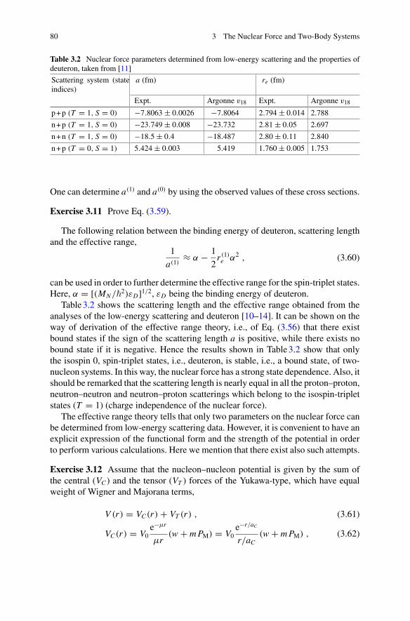
80 3 The Nuclear Force and Two-Body Systems
Table 3.2 Nuclear force parameters determined from low-energy scattering and the properties ofdeuteron, taken from [11]
Scattering system (stateindices)
a (fm) re (fm)
Expt. Argonne v18 Expt. Argonne v18
p+p (T = 1, S = 0) −7.8063 ± 0.0026 −7.8064 2.794 ± 0.014 2.788
n+p (T = 1, S = 0) −23.749 ± 0.008 −23.732 2.81 ± 0.05 2.697
n+n (T = 1, S = 0) −18.5 ± 0.4 −18.487 2.80 ± 0.11 2.840
n+p (T = 0, S = 1) 5.424 ± 0.003 5.419 1.760 ± 0.005 1.753
One can determine a(1) and a(0) by using the observed values of these cross sections.
Exercise 3.11 Prove Eq. (3.59).
The following relation between the binding energy of deuteron, scattering lengthand the effective range,
1
a(1)≈ α − 1
2r (1)
e α2 , (3.60)
can be used in order to further determine the effective range for the spin-triplet states.Here, α = [(MN /�
2)εD]1/2, εD being the binding energy of deuteron.Table3.2 shows the scattering length and the effective range obtained from the
analyses of the low-energy scattering and deuteron [10–14]. It can be shown on theway of derivation of the effective range theory, i.e., of Eq. (3.56) that there existbound states if the sign of the scattering length a is positive, while there exists nobound state if it is negative. Hence the results shown in Table3.2 show that onlythe isospin 0, spin-triplet states, i.e., deuteron, is stable, i.e., a bound state, of two-nucleon systems. In this way, the nuclear force has a strong state dependence. Also, itshould be remarked that the scattering length is nearly equal in all the proton–proton,neutron–neutron and neutron–proton scatterings which belong to the isospin-tripletstates (T = 1) (charge independence of the nuclear force).
The effective range theory tells that only two parameters on the nuclear force canbe determined from low-energy scattering data. However, it is convenient to have anexplicit expression of the functional form and the strength of the potential in orderto perform various calculations. Here we mention that there exist also such attempts.
Exercise 3.12 Assume that the nucleon–nucleon potential is given by the sum ofthe central (VC ) and the tensor (VT ) forces of the Yukawa-type, which have equalweight of Wigner and Majorana terms,
V (r) = VC(r) + VT (r) , (3.61)
VC(r) = V0e−μr
μr(w + m PM) = V0
e−r/aC
r/aC(w + m PM) , (3.62)
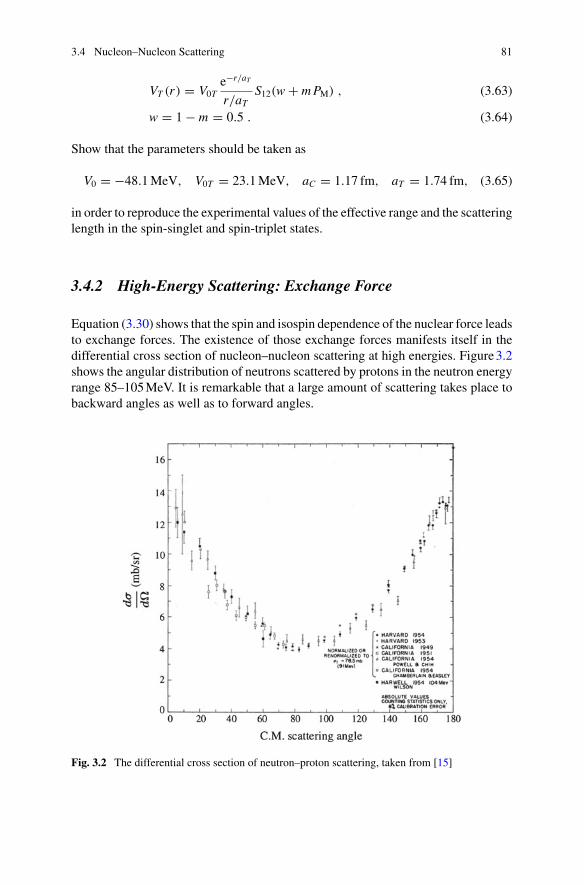
3.4 Nucleon–Nucleon Scattering 81
VT (r) = V0Te−r/aT
r/aTS12(w + m PM) , (3.63)
w = 1 − m = 0.5 . (3.64)
Show that the parameters should be taken as
V0 = −48.1MeV, V0T = 23.1MeV, aC = 1.17 fm, aT = 1.74 fm, (3.65)
in order to reproduce the experimental values of the effective range and the scatteringlength in the spin-singlet and spin-triplet states.
3.4.2 High-Energy Scattering: Exchange Force
Equation (3.30) shows that the spin and isospin dependence of the nuclear force leadsto exchange forces. The existence of those exchange forces manifests itself in thedifferential cross section of nucleon–nucleon scattering at high energies. Figure3.2shows the angular distribution of neutrons scattered by protons in the neutron energyrange 85–105MeV. It is remarkable that a large amount of scattering takes place tobackward angles as well as to forward angles.
Fig. 3.2 The differential cross section of neutron–proton scattering, taken from [15]
82 3 The Nuclear Force and Two-Body Systems
Let us now assume that the nuclear force contains only theWigner force. Since onecan use the Born approximation for high-energy scattering, the scattering amplitudeis given by
fW(θ) = − MN
�2q
∫ ∞
0VW(r)r sin qrdr , (3.66)
withq = 2k sin(θ/2) , (3.67)
to the first order. MN is the nucleon mass and q the wave number correspondingto the momentum transfer. If we assume the Gauss-type for the form factor of thenuclear force,
VW(r) = −VW0 exp
(− r2
R2W
), (3.68)
then we have
fW(θ) = MN
�2qVW0
√π
4R3W exp
[− (q RW)2
4
]. (3.69)
Equation (3.69) shows that the cross section should monotonically decrease towardsbackward angles if the nuclear force consists of the Wigner force alone. This con-tradicts the experimental data shown in Fig. 3.2.
In order to resolve this contradiction, let us assume that the nuclear force containsa Majorana term
VM(r)PM , (3.70)
and examine its effect in the first-order Born approximation. Since the scatteringamplitude is linearly proportional to the nuclear force in the first-order Born approx-imation, it gets an additional term,
fM(θ) = − MN
�2q ′
∫ ∞
0VM(r)r sin q ′rdr (3.71)
with
q′ = ki + k f , (3.72)
q ′ = 2ki sin[(π − θ)/2] , (3.73)
due to the Majorana force. If we assume the Gaussian-type for VM(r) in the sameway as that for the Wigner force, the differential cross section increases with thescattering angle. One can thus explain the large cross section at backward anglesappearing in the experimental data.5
5The Serber force, which is also called the Serber exchange force, is one of such forces. It consistsof the Wigner and the Majorana terms of the same sign with equal weight and is assumed to beproportional to 1 + PM (see Table3.4).
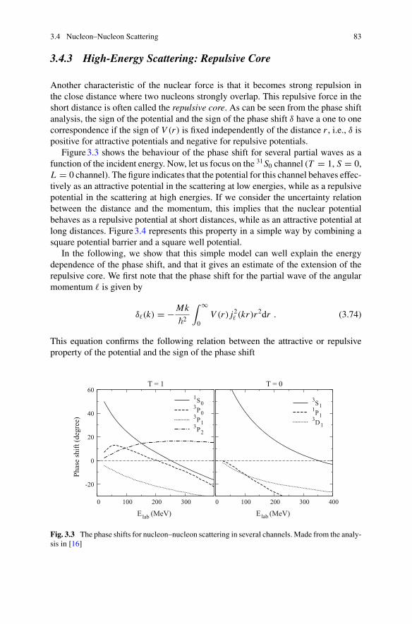
3.4 Nucleon–Nucleon Scattering 83
3.4.3 High-Energy Scattering: Repulsive Core
Another characteristic of the nuclear force is that it becomes strong repulsion inthe close distance where two nucleons strongly overlap. This repulsive force in theshort distance is often called the repulsive core. As can be seen from the phase shiftanalysis, the sign of the potential and the sign of the phase shift δ have a one to onecorrespondence if the sign of V (r) is fixed independently of the distance r , i.e., δ ispositive for attractive potentials and negative for repulsive potentials.
Figure3.3 shows the behaviour of the phase shift for several partial waves as afunction of the incident energy. Now, let us focus on the 31S0 channel (T = 1, S = 0,L = 0 channel). The figure indicates that the potential for this channel behaves effec-tively as an attractive potential in the scattering at low energies, while as a repulsivepotential in the scattering at high energies. If we consider the uncertainty relationbetween the distance and the momentum, this implies that the nuclear potentialbehaves as a repulsive potential at short distances, while as an attractive potential atlong distances. Figure3.4 represents this property in a simple way by combining asquare potential barrier and a square well potential.
In the following, we show that this simple model can well explain the energydependence of the phase shift, and that it gives an estimate of the extension of therepulsive core. We first note that the phase shift for the partial wave of the angularmomentum � is given by
δ�(k) = − Mk
�2
∫ ∞
0V (r) j2� (kr)r2dr . (3.74)
This equation confirms the following relation between the attractive or repulsiveproperty of the potential and the sign of the phase shift
-20
0
20
40
60
0 100 200 300
Phas
e sh
ift (d
egre
e)
E lab (MeV)
T = 1
1S03P03P13P2
0 100 200 300 400
Elab (MeV)
T = 0
3S11P13D1
Fig. 3.3 The phase shifts for nucleon–nucleon scattering in several channels. Made from the analy-sis in [16]
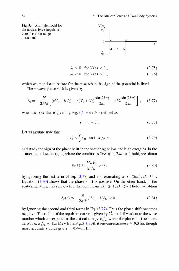
84 3 The Nuclear Force and Two-Body Systems
Fig. 3.4 A simple model forthe nuclear force (repulsivecore plus short rangeattraction)
r
V(r)V1
–V0
0
b
c a
δ� > 0 for V (r) < 0 , (3.75)
δ� < 0 for V (r) > 0 , (3.76)
which we mentioned before for the case when the sign of the potential is fixed.The s-wave phase shift is given by
δ0 = − M
2�2k
[(cV1 − bV0) − c(V1 + V0)
sin(2kc)
2kc+ aV0
sin(2ka)
2ka
], (3.77)
when the potential is given by Fig. 3.4. Here b is defined as
b = a − c . (3.78)
Let us assume now that
V1 >b
cV0 and a � c, (3.79)
and study the sign of the phase shift in the scattering at low and high energies. In thescattering at low energies, where the conditions 2kc � 1, 2ka � 1 hold, we obtain
δ0(k) ≈ MaV0
2�2k> 0 , (3.80)
by ignoring the last term of Eq. (3.77) and approximating as sin(2kc)/2kc ≈ 1.Equation (3.80) shows that the phase shift is positive. On the other hand, in thescattering at high energies, where the conditions 2kc � 1, 2ka � 1 hold, we obtain
δ0(k) ≈ − M
2�2k(cV1 − bV0) < 0 , (3.81)
by ignoring the second and third terms in Eq. (3.77). Thus the phase shift becomesnegative. The radius of the repulsive core c is given by 2kc ≈ 1 if we denote the wavenumber which corresponds to the critical energy Ecr
c.m. where the phase shift becomeszeroby k. Ecr
c.m. ∼ 125MeVfromFig. 3.3, so that one can estimate c ≈ 0.3 fm, thoughmore accurate studies give c = 0.4–0.5 fm.
3.4 Nucleon–Nucleon Scattering 85
3.4.4 Spin Polarization Experiments
Since 1990s, experiments with polarized incident nucleons and/or target nucleusbecame popular. Those experiments are very useful to obtain information on thespin-dependent forces.
Suppose that the force between two nucleons is given by
V = f (r) (V0 + Vσσ 1 · σ 2) . (3.82)
If we define the spin raising and lowering operators by
σ± ≡ σx ± iσy (3.83)
as is often done in the calculations concerning angular momentum, then the innerproduct of the spins can be rewritten as
σ 1 · σ 2 = 1
2(σ1+σ2− + σ1−σ2+) + σ10σ20 . (3.84)
The spin-flip, i.e., the exchange of direction of spins between the incident and targetnucleons, takes place through the first and the second terms on the right-hand sideof Eq. (3.84). Hence one can expect that detailed information on the spin-dependentterms in the nuclear force can be obtained from the experiments related to the spinpolarization.
Exercise 3.13 Study methods to polarize the incident particle or the target nucleus.
Exercise 3.14 Consider the proton–neutron scattering by the following potential,
V = (1 + κ σ 1 · σ 2) f (r) , (3.85)
and assume that the proton and the neutron are in the spin-up and spin-down states,respectively, at the beginning of the scattering. Obtain the probability of exchangingthe direction of spins between the proton and neutron at the end of the scatteringas a function of the strength of the spin-dependent term κ in the first-order Bornapproximation.
3.5 Microscopic Considerations: Meson Theory, QCD
In the meson theory, the force between two nucleons is assumed to work throughthe exchange of various mesons such as π -mesons, ω-mesons and ρ-mesons. In thissection, we discuss the properties of the nuclear force from this point of view.
Let us first derive the force which arises from the exchange of π -mesons. The firststep is to properly postulate a Lagrangian density. Since the π -meson field obeys theKlein–Gordon equation, the corresponding Lagrangian is given by
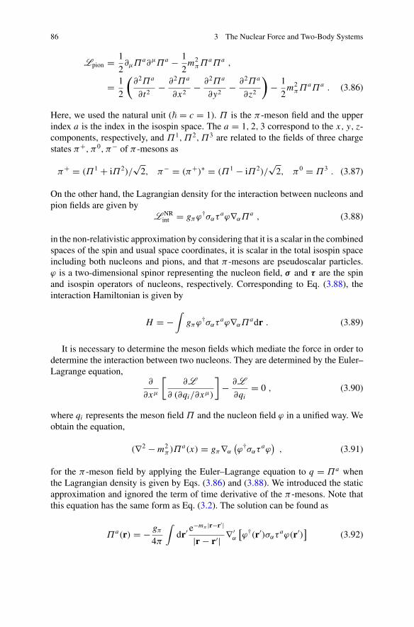
86 3 The Nuclear Force and Two-Body Systems
Lpion = 1
2∂μΠa∂μΠa − 1
2m2
πΠaΠa ,
= 1
2
(∂2Πa
∂t2− ∂2Πa
∂x2− ∂2Πa
∂y2− ∂2Πa
∂z2
)− 1
2m2
πΠaΠa . (3.86)
Here, we used the natural unit (� = c = 1). Π is the π -meson field and the upperindex a is the index in the isospin space. The a = 1, 2, 3 correspond to the x, y, z-components, respectively, and Π1,Π2,Π3 are related to the fields of three chargestates π+, π0, π− of π -mesons as
π+ = (Π1 + iΠ2)/√2, π− = (π+)∗ = (Π1 − iΠ2)/
√2, π0 = Π3 . (3.87)
On the other hand, the Lagrangian density for the interaction between nucleons andpion fields are given by
L NRint = gπϕ†σατ aϕ∇αΠa , (3.88)
in the non-relativistic approximation by considering that it is a scalar in the combinedspaces of the spin and usual space coordinates, it is scalar in the total isospin spaceincluding both nucleons and pions, and that π -mesons are pseudoscalar particles.ϕ is a two-dimensional spinor representing the nucleon field, σ and τ are the spinand isospin operators of nucleons, respectively. Corresponding to Eq. (3.88), theinteraction Hamiltonian is given by
H = −∫
gπϕ†σατ aϕ∇αΠadr . (3.89)
It is necessary to determine the meson fields which mediate the force in order todetermine the interaction between two nucleons. They are determined by the Euler–Lagrange equation,
∂
∂xμ
[∂L
∂ (∂qi/∂xμ)
]− ∂L
∂qi= 0 , (3.90)
where qi represents the meson field Π and the nucleon field ϕ in a unified way. Weobtain the equation,
(∇2 − m2π )Πa(x) = gπ∇α
(ϕ†σατ aϕ
), (3.91)
for the π -meson field by applying the Euler–Lagrange equation to q = Πa whenthe Lagrangian density is given by Eqs. (3.86) and (3.88). We introduced the staticapproximation and ignored the term of time derivative of the π -mesons. Note thatthis equation has the same form as Eq. (3.2). The solution can be found as
Πa(r) = − gπ
4π
∫dr′ e
−mπ |r−r′|
|r − r′| ∇′α
[ϕ†(r′)σατ aϕ(r′)
](3.92)
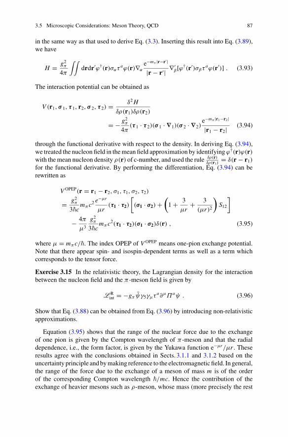
3.5 Microscopic Considerations: Meson Theory, QCD 87
in the same way as that used to derive Eq. (3.3). Inserting this result into Eq. (3.89),we have
H = g2π
4π
∫∫drdr′ϕ†(r)σατ aϕ(r)∇α
e−mπ |r−r′|
|r − r′| ∇′β[ϕ†(r′)σβτ aϕ(r′)] . (3.93)
The interaction potential can be obtained as
V (r1, σ 1, τ 1, r2, σ 2, τ 2) = δ2H
δρ(r1)δρ(r2)
= − g2π
4π(τ 1 · τ 2)(σ 1 · ∇1)(σ 2 · ∇2)
e−mπ |r1−r2|
|r1 − r2| (3.94)
through the functional derivative with respect to the density. In deriving Eq. (3.94),we treated the nucleon field in themean field approximation by identifying ϕ†(r)ϕ(r)with themean nucleon density ρ(r) of c-number, and used the rule δρ(r)
δρ(r1)= δ(r − r1)
for the functional derivative. By performing the differentiation, Eq. (3.94) can berewritten as
V OPEP(r = r1 − r2, σ1, τ1, σ2, τ2)
= g2π
3�cmπc2
e−μr
μr(τ1 · τ2)
[(σ1 · σ2) +
(1 + 3
μr+ 3
(μr)2
)S12
]
− 4π
μ3
g2π
3�cmπc2(τ1 · τ2)(σ1 · σ2)δ(r) , (3.95)
where μ = mπc/�. The index OPEP of V OPEP means one-pion exchange potential.Note that there appear spin- and isospin-dependent terms as well as a term whichcorresponds to the tensor force.
Exercise 3.15 In the relativistic theory, the Lagrangian density for the interactionbetween the nucleon field and the π -meson field is given by
L Rint = −gπ ψγ5γμτ a∂μΠaψ . (3.96)
Show that Eq. (3.88) can be obtained from Eq. (3.96) by introducing non-relativisticapproximations.
Equation (3.95) shows that the range of the nuclear force due to the exchangeof one pion is given by the Compton wavelength of π -meson and that the radialdependence, i.e., the form factor, is given by the Yukawa function e−μr/μr . Theseresults agree with the conclusions obtained in Sects. 3.1.1 and 3.1.2 based on theuncertainty principle and bymaking reference to the electromagnetic field. In general,the range of the force due to the exchange of a meson of mass m is of the orderof the corresponding Compton wavelength �/mc. Hence the contribution of theexchange of heavier mesons such as ρ-meson, whose mass (more precisely the rest
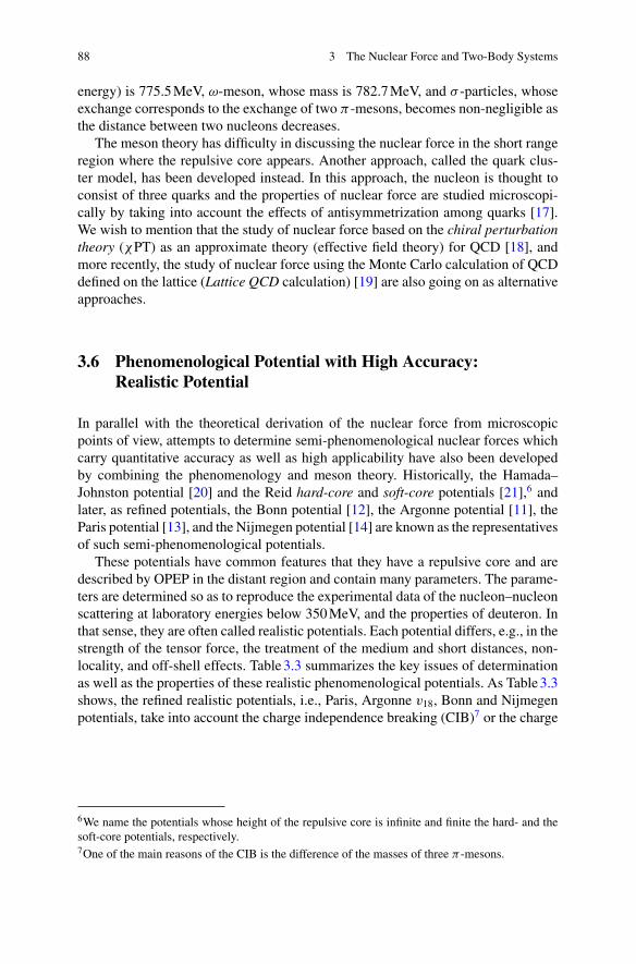
88 3 The Nuclear Force and Two-Body Systems
energy) is 775.5MeV, ω-meson, whose mass is 782.7MeV, and σ -particles, whoseexchange corresponds to the exchange of two π -mesons, becomes non-negligible asthe distance between two nucleons decreases.
The meson theory has difficulty in discussing the nuclear force in the short rangeregion where the repulsive core appears. Another approach, called the quark clus-ter model, has been developed instead. In this approach, the nucleon is thought toconsist of three quarks and the properties of nuclear force are studied microscopi-cally by taking into account the effects of antisymmetrization among quarks [17].We wish to mention that the study of nuclear force based on the chiral perturbationtheory (χPT) as an approximate theory (effective field theory) for QCD [18], andmore recently, the study of nuclear force using the Monte Carlo calculation of QCDdefined on the lattice (Lattice QCD calculation) [19] are also going on as alternativeapproaches.
3.6 Phenomenological Potential with High Accuracy:Realistic Potential
In parallel with the theoretical derivation of the nuclear force from microscopicpoints of view, attempts to determine semi-phenomenological nuclear forces whichcarry quantitative accuracy as well as high applicability have also been developedby combining the phenomenology and meson theory. Historically, the Hamada–Johnston potential [20] and the Reid hard-core and soft-core potentials [21],6 andlater, as refined potentials, the Bonn potential [12], the Argonne potential [11], theParis potential [13], and the Nijmegen potential [14] are known as the representativesof such semi-phenomenological potentials.
These potentials have common features that they have a repulsive core and aredescribed by OPEP in the distant region and contain many parameters. The parame-ters are determined so as to reproduce the experimental data of the nucleon–nucleonscattering at laboratory energies below 350MeV, and the properties of deuteron. Inthat sense, they are often called realistic potentials. Each potential differs, e.g., in thestrength of the tensor force, the treatment of the medium and short distances, non-locality, and off-shell effects. Table3.3 summarizes the key issues of determinationas well as the properties of these realistic phenomenological potentials. As Table3.3shows, the refined realistic potentials, i.e., Paris, Argonne v18, Bonn and Nijmegenpotentials, take into account the charge independence breaking (CIB)7 or the charge
6We name the potentials whose height of the repulsive core is infinite and finite the hard- and thesoft-core potentials, respectively.7One of the main reasons of the CIB is the difference of the masses of three π -mesons.
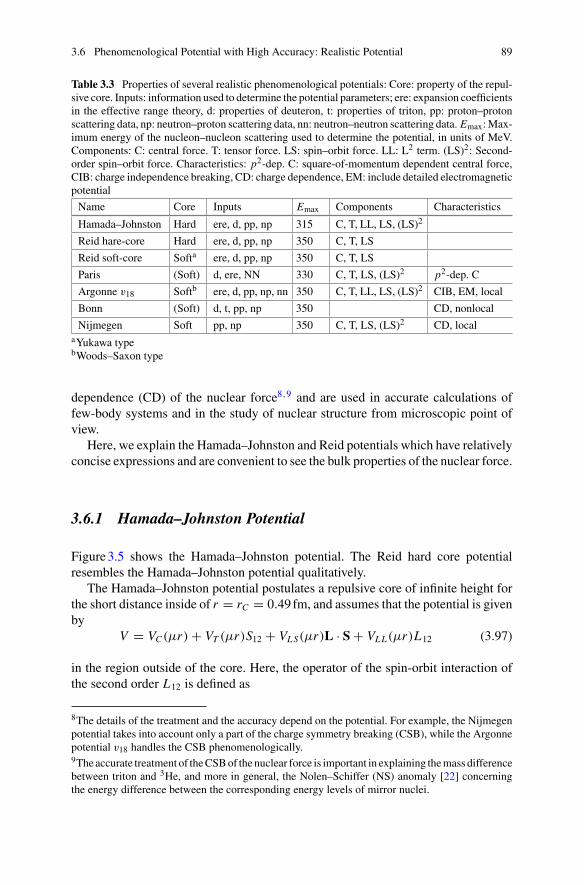
3.6 Phenomenological Potential with High Accuracy: Realistic Potential 89
Table 3.3 Properties of several realistic phenomenological potentials: Core: property of the repul-sive core. Inputs: information used to determine the potential parameters; ere: expansion coefficientsin the effective range theory, d: properties of deuteron, t: properties of triton, pp: proton–protonscattering data, np: neutron–proton scattering data, nn: neutron–neutron scattering data. Emax:Max-imum energy of the nucleon–nucleon scattering used to determine the potential, in units of MeV.Components: C: central force. T: tensor force. LS: spin–orbit force. LL: L2 term. (LS)2: Second-order spin–orbit force. Characteristics: p2-dep. C: square-of-momentum dependent central force,CIB: charge independence breaking, CD: charge dependence, EM: include detailed electromagneticpotential
Name Core Inputs Emax Components Characteristics
Hamada–Johnston Hard ere, d, pp, np 315 C, T, LL, LS, (LS)2
Reid hare-core Hard ere, d, pp, np 350 C, T, LS
Reid soft-core Softa ere, d, pp, np 350 C, T, LS
Paris (Soft) d, ere, NN 330 C, T, LS, (LS)2 p2-dep. C
Argonne v18 Softb ere, d, pp, np, nn 350 C, T, LL, LS, (LS)2 CIB, EM, local
Bonn (Soft) d, t, pp, np 350 CD, nonlocal
Nijmegen Soft pp, np 350 C, T, LS, (LS)2 CD, localaYukawa typebWoods–Saxon type
dependence (CD) of the nuclear force8,9 and are used in accurate calculations offew-body systems and in the study of nuclear structure from microscopic point ofview.
Here, we explain the Hamada–Johnston and Reid potentials which have relativelyconcise expressions and are convenient to see the bulk properties of the nuclear force.
3.6.1 Hamada–Johnston Potential
Figure3.5 shows the Hamada–Johnston potential. The Reid hard core potentialresembles the Hamada–Johnston potential qualitatively.
The Hamada–Johnston potential postulates a repulsive core of infinite height forthe short distance inside of r = rC = 0.49 fm, and assumes that the potential is givenby
V = VC(μr) + VT (μr)S12 + VL S(μr)L · S + VL L(μr)L12 (3.97)
in the region outside of the core. Here, the operator of the spin-orbit interaction ofthe second order L12 is defined as
8The details of the treatment and the accuracy depend on the potential. For example, the Nijmegenpotential takes into account only a part of the charge symmetry breaking (CSB), while the Argonnepotential v18 handles the CSB phenomenologically.9The accurate treatment of theCSBof the nuclear force is important in explaining themass differencebetween triton and 3He, and more in general, the Nolen–Schiffer (NS) anomaly [22] concerningthe energy difference between the corresponding energy levels of mirror nuclei.
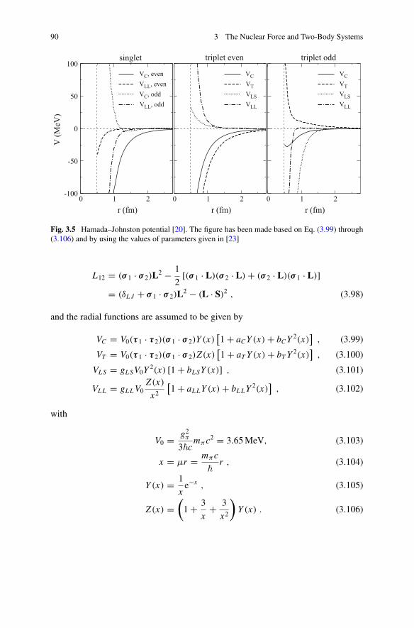
90 3 The Nuclear Force and Two-Body Systems
-100
-50
0
50
100
0 1 2
V (M
eV)
r (fm)
singlet
VC, evenVLL, evenVC, oddVLL, odd
0 1 2r (fm)
triplet even
VCVTVLSVLL
0 1 2r (fm)
triplet odd
VCVTVLSVLL
Fig. 3.5 Hamada–Johnston potential [20]. The figure has been made based on Eq. (3.99) through(3.106) and by using the values of parameters given in [23]
L12 = (σ 1 · σ 2)L2 − 1
2[(σ 1 · L)(σ 2 · L) + (σ 2 · L)(σ 1 · L)]
= (δL J + σ 1 · σ 2)L2 − (L · S)2 , (3.98)
and the radial functions are assumed to be given by
VC = V0(τ 1 · τ 2)(σ 1 · σ 2)Y (x)[1 + aC Y (x) + bC Y 2(x)
], (3.99)
VT = V0(τ 1 · τ 2)(σ 1 · σ 2)Z(x)[1 + aT Y (x) + bT Y 2(x)
], (3.100)
VL S = gL S V0Y 2(x) [1 + bL SY (x)] , (3.101)
VL L = gL L V0Z(x)
x2
[1 + aL LY (x) + bL LY 2(x)
], (3.102)
with
V0 = g2π
3�cmπc2 = 3.65MeV, (3.103)
x = μr = mπc
�r , (3.104)
Y (x) = 1
xe−x , (3.105)
Z(x) =(1 + 3
x+ 3
x2
)Y (x) . (3.106)
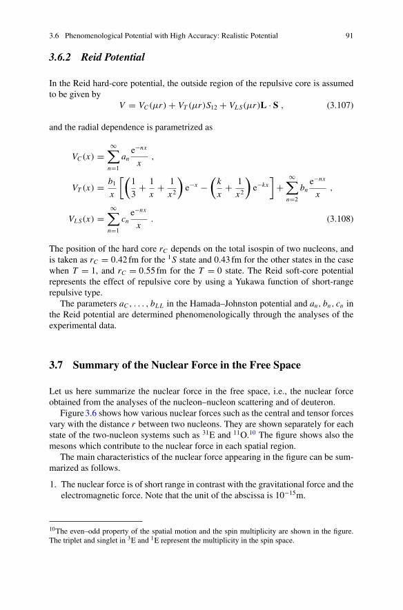
3.6 Phenomenological Potential with High Accuracy: Realistic Potential 91
3.6.2 Reid Potential
In the Reid hard-core potential, the outside region of the repulsive core is assumedto be given by
V = VC(μr) + VT (μr)S12 + VL S(μr)L · S , (3.107)
and the radial dependence is parametrized as
VC(x) =∞∑
n=1
ane−nx
x,
VT (x) = b1x
[(1
3+ 1
x+ 1
x2
)e−x −
(k
x+ 1
x2
)e−kx
]+
∞∑n=2
bne−nx
x,
VL S(x) =∞∑
n=1
cne−nx
x. (3.108)
The position of the hard core rC depends on the total isospin of two nucleons, andis taken as rC = 0.42 fm for the 1S state and 0.43 fm for the other states in the casewhen T = 1, and rC = 0.55 fm for the T = 0 state. The Reid soft-core potentialrepresents the effect of repulsive core by using a Yukawa function of short-rangerepulsive type.
The parameters aC , . . . , bL L in the Hamada–Johnston potential and an, bn, cn inthe Reid potential are determined phenomenologically through the analyses of theexperimental data.
3.7 Summary of the Nuclear Force in the Free Space
Let us here summarize the nuclear force in the free space, i.e., the nuclear forceobtained from the analyses of the nucleon–nucleon scattering and of deuteron.
Figure3.6 shows how various nuclear forces such as the central and tensor forcesvary with the distance r between two nucleons. They are shown separately for eachstate of the two-nucleon systems such as 31E and 11O.10 The figure shows also themesons which contribute to the nuclear force in each spatial region.
The main characteristics of the nuclear force appearing in the figure can be sum-marized as follows.
1. The nuclear force is of short range in contrast with the gravitational force and theelectromagnetic force. Note that the unit of the abscissa is 10−15m.
10The even–odd property of the spatial motion and the spin multiplicity are shown in the figure.The triplet and singlet in 3E and 1E represent the multiplicity in the spin space.
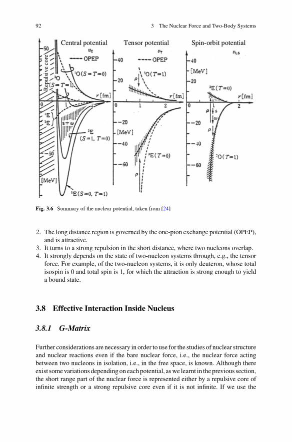
92 3 The Nuclear Force and Two-Body Systems
Fig. 3.6 Summary of the nuclear potential, taken from [24]
2. The long distance region is governed by the one-pion exchange potential (OPEP),and is attractive.
3. It turns to a strong repulsion in the short distance, where two nucleons overlap.4. It strongly depends on the state of two-nucleon systems through, e.g., the tensor
force. For example, of the two-nucleon systems, it is only deuteron, whose totalisospin is 0 and total spin is 1, for which the attraction is strong enough to yielda bound state.
3.8 Effective Interaction Inside Nucleus
3.8.1 G-Matrix
Further considerations are necessary in order to use for the studies of nuclear structureand nuclear reactions even if the bare nuclear force, i.e., the nuclear force actingbetween two nucleons in isolation, i.e., in the free space, is known. Although thereexist somevariations dependingon eachpotential, aswe learnt in the previous section,the short range part of the nuclear force is represented either by a repulsive core ofinfinite strength or a strong repulsive core even if it is not infinite. If we use the
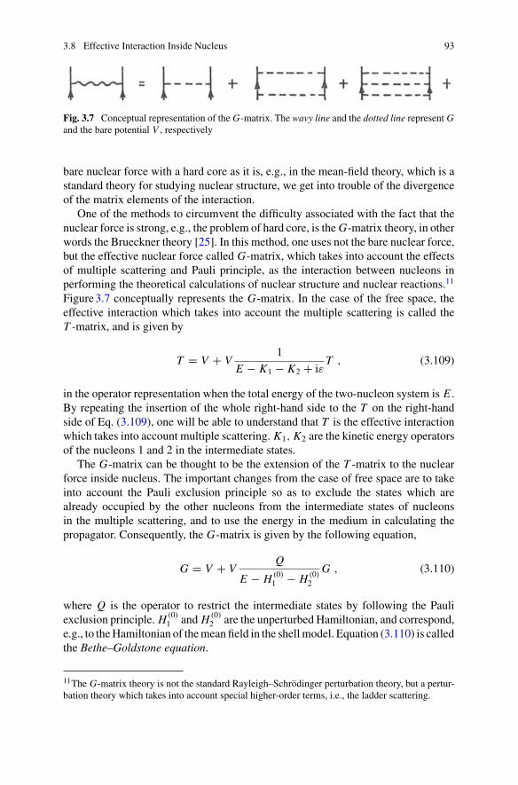
3.8 Effective Interaction Inside Nucleus 93
Fig. 3.7 Conceptual representation of the G-matrix. The wavy line and the dotted line represent Gand the bare potential V , respectively
bare nuclear force with a hard core as it is, e.g., in the mean-field theory, which is astandard theory for studying nuclear structure, we get into trouble of the divergenceof the matrix elements of the interaction.
One of the methods to circumvent the difficulty associated with the fact that thenuclear force is strong, e.g., the problem of hard core, is the G-matrix theory, in otherwords the Brueckner theory [25]. In this method, one uses not the bare nuclear force,but the effective nuclear force called G-matrix, which takes into account the effectsof multiple scattering and Pauli principle, as the interaction between nucleons inperforming the theoretical calculations of nuclear structure and nuclear reactions.11
Figure3.7 conceptually represents the G-matrix. In the case of the free space, theeffective interaction which takes into account the multiple scattering is called theT -matrix, and is given by
T = V + V1
E − K1 − K2 + iεT , (3.109)
in the operator representation when the total energy of the two-nucleon system is E .By repeating the insertion of the whole right-hand side to the T on the right-handside of Eq. (3.109), one will be able to understand that T is the effective interactionwhich takes into account multiple scattering. K1, K2 are the kinetic energy operatorsof the nucleons 1 and 2 in the intermediate states.
The G-matrix can be thought to be the extension of the T -matrix to the nuclearforce inside nucleus. The important changes from the case of free space are to takeinto account the Pauli exclusion principle so as to exclude the states which arealready occupied by the other nucleons from the intermediate states of nucleonsin the multiple scattering, and to use the energy in the medium in calculating thepropagator. Consequently, the G-matrix is given by the following equation,
G = V + VQ
E − H (0)1 − H (0)
2
G , (3.110)
where Q is the operator to restrict the intermediate states by following the Pauliexclusion principle. H (0)
1 and H (0)2 are the unperturbed Hamiltonian, and correspond,
e.g., to theHamiltonian of themean field in the shellmodel. Equation (3.110) is calledthe Bethe–Goldstone equation.
11The G-matrix theory is not the standard Rayleigh–Schrödinger perturbation theory, but a pertur-bation theory which takes into account special higher-order terms, i.e., the ladder scattering.
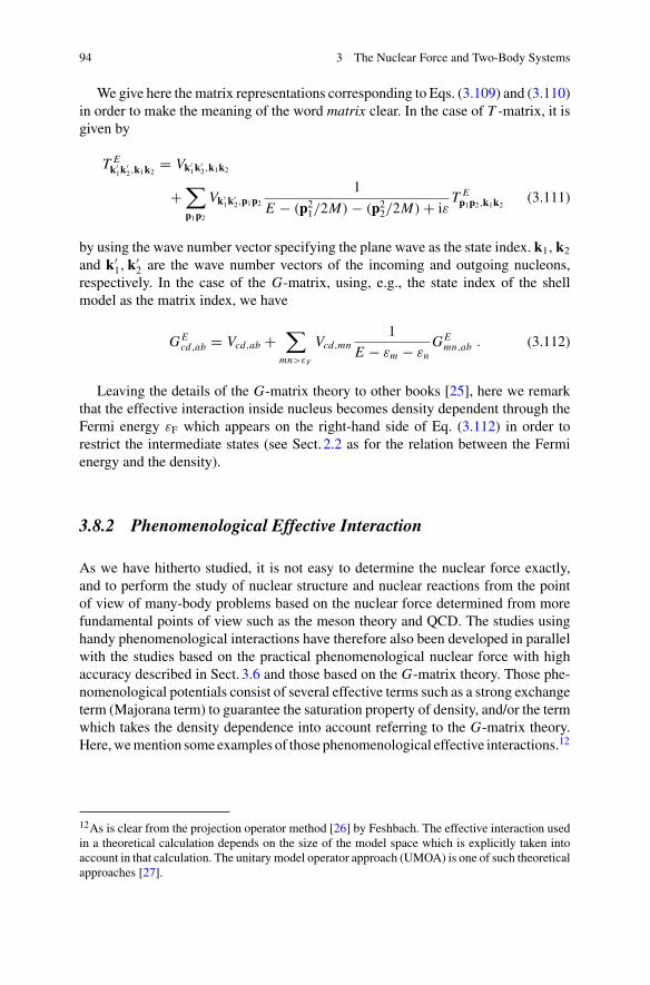
94 3 The Nuclear Force and Two-Body Systems
We give here thematrix representations corresponding to Eqs. (3.109) and (3.110)in order to make the meaning of the word matrix clear. In the case of T -matrix, it isgiven by
T Ek′1k
′2,k1k2
= Vk′1k
′2,k1k2
+∑p1p2
Vk′1k
′2,p1p2
1
E − (p21/2M) − (p22/2M) + iεT Ep1p2,k1k2
(3.111)
by using the wave number vector specifying the plane wave as the state index. k1,k2
and k′1,k
′2 are the wave number vectors of the incoming and outgoing nucleons,
respectively. In the case of the G-matrix, using, e.g., the state index of the shellmodel as the matrix index, we have
G Ecd,ab = Vcd,ab +
∑mn>εF
Vcd,mn1
E − εm − εnG E
mn,ab . (3.112)
Leaving the details of the G-matrix theory to other books [25], here we remarkthat the effective interaction inside nucleus becomes density dependent through theFermi energy εF which appears on the right-hand side of Eq. (3.112) in order torestrict the intermediate states (see Sect. 2.2 as for the relation between the Fermienergy and the density).
3.8.2 Phenomenological Effective Interaction
As we have hitherto studied, it is not easy to determine the nuclear force exactly,and to perform the study of nuclear structure and nuclear reactions from the pointof view of many-body problems based on the nuclear force determined from morefundamental points of view such as the meson theory and QCD. The studies usinghandy phenomenological interactions have therefore also been developed in parallelwith the studies based on the practical phenomenological nuclear force with highaccuracy described in Sect. 3.6 and those based on the G-matrix theory. Those phe-nomenological potentials consist of several effective terms such as a strong exchangeterm (Majorana term) to guarantee the saturation property of density, and/or the termwhich takes the density dependence into account referring to the G-matrix theory.Here,wemention some examples of those phenomenological effective interactions.12
12As is clear from the projection operator method [26] by Feshbach. The effective interaction usedin a theoretical calculation depends on the size of the model space which is explicitly taken intoaccount in that calculation. The unitary model operator approach (UMOA) is one of such theoreticalapproaches [27].
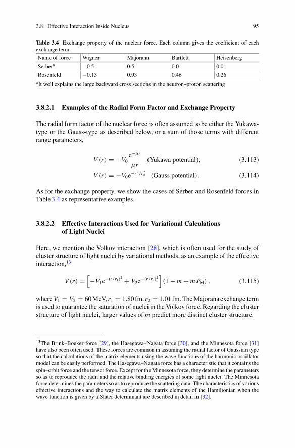
3.8 Effective Interaction Inside Nucleus 95
Table 3.4 Exchange property of the nuclear force. Each column gives the coefficient of eachexchange term
Name of force Wigner Majorana Bartlett Heisenberg
Serbera 0.5 0.5 0.0 0.0
Rosenfeld −0.13 0.93 0.46 0.26aIt well explains the large backward cross sections in the neutron–proton scattering
3.8.2.1 Examples of the Radial Form Factor and Exchange Property
The radial form factor of the nuclear force is often assumed to be either the Yukawa-type or the Gauss-type as described below, or a sum of those terms with differentrange parameters,
V (r) = −V0e−μr
μr(Yukawa potential), (3.113)
V (r) = −V0e−r2/r20 (Gauss potential). (3.114)
As for the exchange property, we show the cases of Serber and Rosenfeld forces inTable3.4 as representative examples.
3.8.2.2 Effective Interactions Used for Variational Calculationsof Light Nuclei
Here, we mention the Volkov interaction [28], which is often used for the study ofcluster structure of light nuclei by variational methods, as an example of the effectiveinteraction,13
V (r) =[−V1e
−(r/r1)2 + V2e−(r/r2)2
](1 − m + m PM) , (3.115)
whereV1 = V2 = 60MeV, r1 = 1.80 fm, r2 = 1.01 fm.TheMajorana exchange termis used to guarantee the saturation of nuclei in the Volkov force. Regarding the clusterstructure of light nuclei, larger values of m predict more distinct cluster structure.
13The Brink–Boeker force [29], the Hasegawa–Nagata force [30], and the Minnesota force [31]have also been often used. These forces are common in assuming the radial factor of Gaussian typeso that the calculations of the matrix elements using the wave functions of the harmonic oscillatormodel can be easily performed. The Hasegawa–Nagata force has a characteristic that it contains thespin–orbit force and the tensor force. Except for theMinnesota force, they determine the parametersso as to reproduce the radii and the relative binding energies of some light nuclei. The Minnesotaforce determines the parameters so as to reproduce the scattering data. The characteristics of variouseffective interactions and the way to calculate the matrix elements of the Hamiltonian when thewave function is given by a Slater determinant are described in detail in [32].
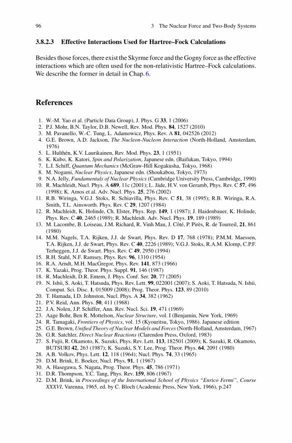
96 3 The Nuclear Force and Two-Body Systems
3.8.2.3 Effective Interactions Used for Hartree–Fock Calculations
Besides those forces, there exist the Skyrme force and theGogny force as the effectiveinteractions which are often used for the non-relativistic Hartree–Fock calculations.We describe the former in detail in Chap. 6.
References
1. W.-M. Yao et al. (Particle Data Group), J. Phys. G 33, 1 (2006)2. P.J. Mohr, B.N. Taylor, D.B. Newell, Rev. Mod. Phys. 84, 1527 (2010)3. M. Pavanello, W.-C. Tung, L. Adamowicz, Phys. Rev. A 81, 042526 (2012)4. G.E. Brown, A.D. Jackson, The Nucleon-Nucleon Interaction (North-Holland, Amsterdam,
1976)5. L. Hulthén, K.V. Laurikainen, Rev. Mod. Phys. 23, 1 (1951)6. K. Kubo, K. Katori, Spin and Polarization, Japanese edn. (Baifukan, Tokyo, 1994)7. L.I. Schiff, Quantum Mechanics (McGraw-Hill Kogakusha, Tokyo, 1968)8. M. Nogami, Nuclear Physics, Japanese edn. (Shoukabou, Tokyo, 1973)9. N.A. Jelly, Fundamentals of Nuclear Physics (Cambridge University Press, Cambridge, 1990)10. R. Machleidt, Nucl. Phys. A 689, 11c (2001); L. Jäde, H.V. von Geramb, Phys. Rev. C 57, 496
(1998); K. Amos et al. Adv. Nucl. Phys. 25, 276 (2002)11. R.B. Wiringa, V.G.J. Stoks, R. Schiavilla, Phys. Rev. C 51, 38 (1995); R.B. Wiringa, R.A.
Smith, T.L. Ainsworth. Phys. Rev. C 29, 1207 (1984)12. R. Machleidt, K. Holinde, Ch. Elster, Phys. Rep. 149, 1 (1987); J. Haidenbauer, K. Holinde,
Phys. Rev. C 40, 2465 (1989); R. Machleidt. Adv. Nucl. Phys. 19, 189 (1989)13. M. Lacombe, B. Loiseau, J.M. Richard, R. Vinh Mau, J. Côté, P. Pirès, R. de Tourreil, 21, 861
(1980)14. M.M. Nagels, T.A. Rijken, J.J. de Swart, Phys. Rev. D 17, 768 (1978); P.M.M. Maessen,
T.A. Rijken, J.J. de Swart, Phys. Rev. C 40, 2226 (1989); V.G.J. Stoks, R.A.M. Klomp, C.P.F.Terheggen, J.J. de Swart. Phys. Rev. C 49, 2950 (1994)
15. R.H. Stahl, N.F. Ramsey, Phys. Rev. 96, 1310 (1954)16. R.A. Arndt, M.H. MacGregor, Phys. Rev. 141, 873 (1966)17. K. Yazaki, Prog. Theor. Phys. Suppl. 91, 146 (1987)18. R. Machleidt, D.R. Entem, J. Phys. Conf. Ser. 20, 77 (2005)19. N. Ishii, S. Aoki, T. Hatsuda, Phys. Rev. Lett. 99, 022001 (2007); S. Aoki, T. Hatsuda, N. Ishii,
Comput. Sci. Disc. 1, 015009 (2008); Prog. Theor. Phys. 123, 89 (2010)20. T. Hamada, I.D. Johnston, Nucl. Phys. A 34, 382 (1962)21. P.V. Reid, Ann. Phys. 50, 411 (1968)22. J.A. Nolen, J.P. Schiffer, Ann. Rev. Nucl. Sci. 19, 471 (1969)23. Aage Bohr, Ben R. Mottelson, Nuclear Structure, vol. I (Benjamin, New York, 1969)24. R. Tamagaki, Frontiers of Physics, vol. 15 (Kyouritsu, Tokyo, 1986). Japanese edition25. G.E. Brown,Unified Theory of Nuclear Models and Forces (North-Holland, Amsterdam, 1967)26. G.R. Satchler, Direct Nuclear Reactions (Clarendon Press, Oxford, 1983)27. S. Fujii, R. Okamoto, K. Suzuki, Phys. Rev. Lett. 113, 182501 (2009); K. Suzuki, R. Okamoto,
BUTSURI 42, 263 (1987); K. Suzuki, S.Y. Lee, Prog. Theor. Phys. 64, 2091 (1980)28. A.B. Volkov, Phys. Lett. 12, 118 (1964); Nucl. Phys. 74, 33 (1965)29. D.M. Brink, E. Boeker, Nucl. Phys. 91, 1 (1967)30. A. Hasegawa, S. Nagata, Prog. Theor. Phys. 45, 786 (1971)31. D.R. Thompson, Y.C. Tang, Phys. Rev. 159, 806 (1967)32. D.M. Brink, in Proceedings of the International School of Physics “Enrico Fermi”, Course
XXXVI, Varenna, 1965, ed. by C. Bloch (Academic Press, New York, 1966), p.247
Chapter 4Interaction with Electromagnetic Field:Electromagnetic Moments
Abstract As mentioned in Chap.1, by measuring the magnetic moment of proton,Stern showed that the proton is not an ideal point particle which can be describedby the Dirac equation. Also, we learnt in Chap. 3 that the magnetic moment ofdeuteron tells that deuteron is in the spin-triplet and isospin-singlet states, and thatone can get information on the magnitude of the tensor force through the admixtureof the D-state in deuteron. In this way, the electromagnetic properties of nucleiprovide valuable information on the structure of nucleons and nuclei. Also, theinteraction of nuclei with the radiation field leads to the emission and absorptionof a γ -ray, governs the lifetime of each energy level, and provides information onthe nuclear structure as well as nuclear collective motions through the strength ofthe electromagnetic transitions between nuclear levels. Furthermore, the measure-ment of the angular correlation between the cascade γ -rays enables us to determinethe spin of each energy level. The electromagnetic transitions play an importantrole also in the synthesis of elements through, e.g., the radiative neutron capture(see Cottingham and Greenwood, An Introduction to Nuclear Physics, 2nd edn.(Cambridge University Press, Cambridge, 2001); Thompson and Nunes, NuclearReactions for Astrophysics: Principles, Calculation andApplications of Low-EnergyReactions (Cambridge University Press, Cambridge, 2009) [1, 2]). In this chapterwe learn the electromagnetic moments such as the magnetic dipole moment and thequadrupole moment which provides important information on the nuclear shape. Theelectromagnetic transitions by emitting γ -rays will be discussed in Sect. 8.3 after welearn about nuclear structure in Chaps. 5 and 7.
4.1 Hamiltonian of the Electromagnetic Interactionand Electromagnetic Multipole Moments
The Hamiltonian of the interaction between a nucleus and the electromagnetic fieldis given by
Hem =∫
ρC(r)ϕ(r)dr − 1
c
∫j(r) · A(r)dr , (4.1)
© Springer Japan 2017N. Takigawa and K. Washiyama, Fundamentals of Nuclear Physics,DOI 10.1007/978-4-431-55378-6_4
97
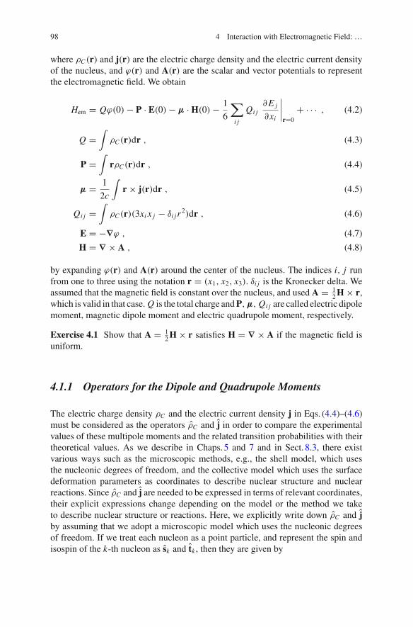
98 4 Interaction with Electromagnetic Field: …
where ρC(r) and j(r) are the electric charge density and the electric current densityof the nucleus, and ϕ(r) and A(r) are the scalar and vector potentials to representthe electromagnetic field. We obtain
Hem = Qϕ(0) − P · E(0) − μ · H(0) − 1
6
∑i j
Qi j∂E j
∂xi
∣∣∣∣r=0
+ · · · , (4.2)
Q =∫
ρC(r)dr , (4.3)
P =∫
rρC(r)dr , (4.4)
μ = 1
2c
∫r × j(r)dr , (4.5)
Qi j =∫
ρC(r)(3xi x j − δi j r2)dr , (4.6)
E = −∇ϕ , (4.7)
H = ∇ × A , (4.8)
by expanding ϕ(r) and A(r) around the center of the nucleus. The indices i, j runfrom one to three using the notation r = (x1, x2, x3). δi j is the Kronecker delta. Weassumed that the magnetic field is constant over the nucleus, and used A = 1
2H × r,which is valid in that case. Q is the total charge andP,μ, Qi j are called electric dipolemoment, magnetic dipole moment and electric quadrupole moment, respectively.
Exercise 4.1 Show that A = 12H × r satisfies H = ∇ × A if the magnetic field is
uniform.
4.1.1 Operators for the Dipole and Quadrupole Moments
The electric charge density ρC and the electric current density j in Eqs. (4.4)–(4.6)must be considered as the operators ρC and j in order to compare the experimentalvalues of these multipole moments and the related transition probabilities with theirtheoretical values. As we describe in Chaps. 5 and 7 and in Sect. 8.3, there existvarious ways such as the microscopic methods, e.g., the shell model, which usesthe nucleonic degrees of freedom, and the collective model which uses the surfacedeformation parameters as coordinates to describe nuclear structure and nuclearreactions. Since ρC and j are needed to be expressed in terms of relevant coordinates,their explicit expressions change depending on the model or the method we taketo describe nuclear structure or reactions. Here, we explicitly write down ρC and jby assuming that we adopt a microscopic model which uses the nucleonic degreesof freedom. If we treat each nucleon as a point particle, and represent the spin andisospin of the k-th nucleon as sk and tk , then they are given by

4.1 Hamiltonian of the Electromagnetic Interaction … 99
ρ(r) = e∑k
(1
2− tz(k)
)δ(r − rk) , (4.9)
j(r) = e∑k
(1
2− tz(k)
)1
2
[vkδ(r − rk) + δ(r − rk)vk
]
+ e�
2MN
∑k
gs(k)∇ × skδ(r − rk) , (4.10)
where
vk = i
�
[H , rk
]∼ 1
mpk , (4.11)
gs(k) ≡ 1
2[gn(k) + gp(k)] + tz(k)[gn(k) − gp(k)] . (4.12)
gs is called the spin g-factor. We use the values of the anomalous magnetic momentsgn = 2μn/μN = −3.826 and gp = 2μp/μN = 5.586 discussed in Chap.1 for gnand gp. The first and second terms on the right-hand side of Eq. (4.10) are calledthe convection current and the magnetization current, respectively. The former isthe usual electric current due to the orbital motion of protons, while the latter theelectric current associated with the magnetic moments of protons and neutrons.Equation (4.10) can be derived from the Dirac equation, which the Fermi particleshould obey, by making non-relativistic approximation.
Exercise 4.2 In the Dirac theory, the current density is given by j k = cψ†αkψ withαk ≡ (
0 σ k
σ k 0
). On the other hand, the two-dimensional spinor χ representing the
third and fourth components of ψ , i.e., the small components if the velocity is small,can be approximated as χ ≈ (σ · p/2mc)ϕ by using the first and second componentsϕ if the velocity of the particle is sufficiently smaller than the light velocity. Notingthese properties, derive Eq. (4.10).
By inserting Eqs. (4.9) and (4.10) into Eqs. (4.3)–(4.6), we obtain
Q = e∑k
(1
2− tz(k)
), (4.13)
P = e∑k
(1
2− tz(k)
)rk , (4.14)
μ = 1
2c
∫r ×
[jc(r) + jmag(r)
]dr ≡ μconvection + μmag , (4.15)
μconvection = μN
∑k
(1
2− tz(k)
)�k , (4.16)
μmag = μN
∑k
gs(k)sk , (4.17)
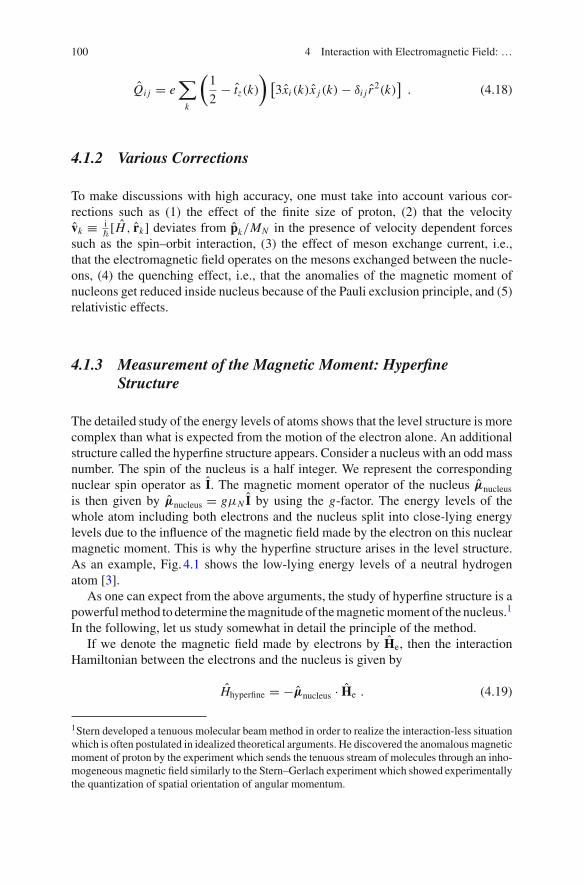
100 4 Interaction with Electromagnetic Field: …
Qi j = e∑k
(1
2− tz(k)
) [3xi (k)x j (k) − δi j r
2(k)]
. (4.18)
4.1.2 Various Corrections
To make discussions with high accuracy, one must take into account various cor-rections such as (1) the effect of the finite size of proton, (2) that the velocityvk ≡ i
�[H , rk] deviates from pk/MN in the presence of velocity dependent forces
such as the spin–orbit interaction, (3) the effect of meson exchange current, i.e.,that the electromagnetic field operates on the mesons exchanged between the nucle-ons, (4) the quenching effect, i.e., that the anomalies of the magnetic moment ofnucleons get reduced inside nucleus because of the Pauli exclusion principle, and (5)relativistic effects.
4.1.3 Measurement of the Magnetic Moment: HyperfineStructure
The detailed study of the energy levels of atoms shows that the level structure is morecomplex than what is expected from the motion of the electron alone. An additionalstructure called the hyperfine structure appears. Consider a nucleus with an oddmassnumber. The spin of the nucleus is a half integer. We represent the correspondingnuclear spin operator as I. The magnetic moment operator of the nucleus μnucleus
is then given by μnucleus = gμN I by using the g-factor. The energy levels of thewhole atom including both electrons and the nucleus split into close-lying energylevels due to the influence of the magnetic field made by the electron on this nuclearmagnetic moment. This is why the hyperfine structure arises in the level structure.As an example, Fig. 4.1 shows the low-lying energy levels of a neutral hydrogenatom [3].
As one can expect from the above arguments, the study of hyperfine structure is apowerfulmethod to determine themagnitude of themagneticmoment of the nucleus.1
In the following, let us study somewhat in detail the principle of the method.If we denote the magnetic field made by electrons by He, then the interaction
Hamiltonian between the electrons and the nucleus is given by
Hhyperfine = −μnucleus · He . (4.19)
1Stern developed a tenuous molecular beam method in order to realize the interaction-less situationwhich is often postulated in idealized theoretical arguments. He discovered the anomalous magneticmoment of proton by the experiment which sends the tenuous stream of molecules through an inho-mogeneous magnetic field similarly to the Stern–Gerlach experiment which showed experimentallythe quantization of spatial orientation of angular momentum.
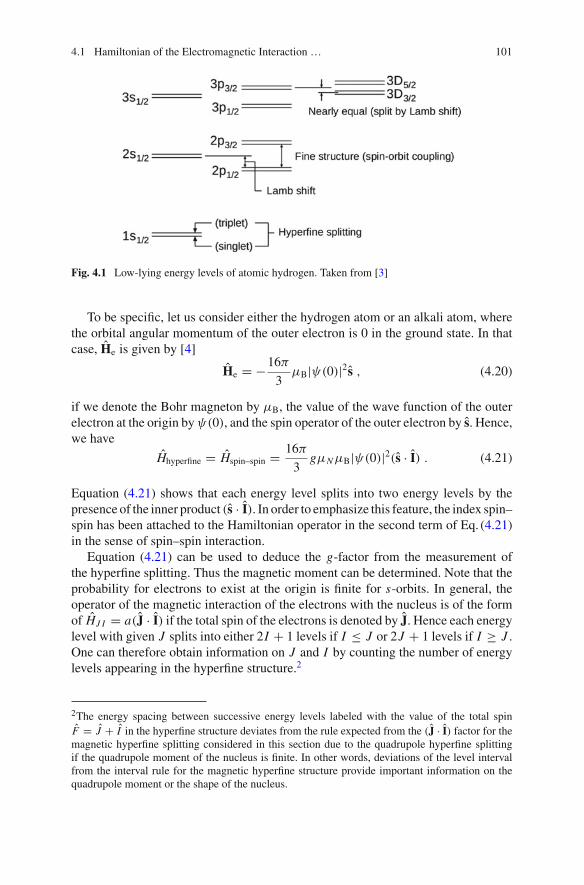
4.1 Hamiltonian of the Electromagnetic Interaction … 101
Fig. 4.1 Low-lying energy levels of atomic hydrogen. Taken from [3]
To be specific, let us consider either the hydrogen atom or an alkali atom, wherethe orbital angular momentum of the outer electron is 0 in the ground state. In thatcase, He is given by [4]
He = −16π
3μB|ψ(0)|2s , (4.20)
if we denote the Bohr magneton by μB, the value of the wave function of the outerelectron at the origin byψ(0), and the spin operator of the outer electron by s. Hence,we have
Hhyperfine = Hspin–spin = 16π
3gμNμB|ψ(0)|2(s · I) . (4.21)
Equation (4.21) shows that each energy level splits into two energy levels by thepresence of the inner product (s · I). In order to emphasize this feature, the index spin–spin has been attached to the Hamiltonian operator in the second term of Eq. (4.21)in the sense of spin–spin interaction.
Equation (4.21) can be used to deduce the g-factor from the measurement ofthe hyperfine splitting. Thus the magnetic moment can be determined. Note that theprobability for electrons to exist at the origin is finite for s-orbits. In general, theoperator of the magnetic interaction of the electrons with the nucleus is of the formof HJ I = a(J · I) if the total spin of the electrons is denoted by J. Hence each energylevel with given J splits into either 2I + 1 levels if I ≤ J or 2J + 1 levels if I ≥ J .One can therefore obtain information on J and I by counting the number of energylevels appearing in the hyperfine structure.2
2The energy spacing between successive energy levels labeled with the value of the total spinF = J + I in the hyperfine structure deviates from the rule expected from the (J · I) factor for themagnetic hyperfine splitting considered in this section due to the quadrupole hyperfine splittingif the quadrupole moment of the nucleus is finite. In other words, deviations of the level intervalfrom the interval rule for the magnetic hyperfine structure provide important information on thequadrupole moment or the shape of the nucleus.
102 4 Interaction with Electromagnetic Field: …
Exercise 4.3 Show that the strength of themagnetic fieldmade by the electron at theposition of nucleus is 105–106 Gauss depending on the species of atom by obtainingthe magnitude of |ψ(0)|2 as a function of the atomic number Z and the principalquantum number n by using the wave function of the hydrogen atom.
Exercise 4.4 Besides the study of hyperfine structure, there exist various methodsto measure the magnetic moment such as the method of nuclear magnetic resonance,molecular beam method, Rabi’s molecular beam resonance method (Rabi’s refocusmethod) and the perturbed angular correlation method (PAC). Study the principleand features of each method.
4.2 Electromagnetic Multipole Operators
It is convenient to begin with the generalized definition in order to discuss in aunified way not only the low-order moments introduced in Sect. 4.1.1, but also allthe electromagnetic properties of nuclei including higher-order multipole momentsas well as the emission and absorption of photons.
Let us first consider the static electric potential φ(r) made by a nucleus in the fardistance from the nucleus. We denote the proton density inside the nucleus by ρp(r).Using the formula of the multipole expansion of 1/|r − r′| for the case of r > r ′, wehave
φ(r) = e∫
ρp(r′)1
|r − r′|dr′
= 4πe
r
∑ m
1
2 + 1
[∫dr′ρp(r′)(r ′) Y m(Ωr ′)
]1
r Y ∗
m(Ωr ) . (4.22)
If we define the μ component of the electric multipole operator by
Qλμ =∫
ρp(r)rλYλμ(Ωr )dr , (4.23)
then, the static electric potential is given by
φ(r) = 4πe∑ m
Q m
2 + 1
Y ∗ m(Ωr )
r +1. (4.24)
Similarly we define the μ component of the magnetic multipole operator by
Mλμ ≡∫
μ(r) · ∇(rλYλμ(Ωr ))dr (4.25)
= 1
c(λ + 1)
∫[r × j(r)] · [∇rλYλμ(Ωr )
]dr . (4.26)
4.2 Electromagnetic Multipole Operators 103
We used A · (B × C) = B · (C × A) = C · (A × B) and the relationship j(r) =c∇ × μ(r) in order to transform from Eq. (4.25) to (4.26).
By inserting the results of Eqs. (4.9) and (4.10) into Eqs. (4.23) and (4.26), weobtain the expressions for the electromagnetic multipole operators in terms of nucle-onic coordinates as
Qλμ = e∑k
(1
2− tz(k)
)rλk Yλμ(θk, ϕk) , (4.27)
Mλμ = μN
∑k
[gs(k)sk + 2
λ + 1g (k)�k
]· [∇rλYλμ(θ, ϕ)
]r=rk
. (4.28)
4.3 Properties of the Electromagnetic Multipole Operators
4.3.1 Parity, Tensor Property and Selection Rule
4.3.1.1 Parity
If we denote the operator of the Parity transformation, which inverts all spatial coor-dinates, by P , and represent the coordinate using the polar coordinates (r, θ, ϕ), thedefinition of P ,
P(r, θ, ϕ)P−1 ≡ (r, π − θ, ϕ + π) , (4.29)
leads to
PYλμ(r, θ, ϕ)P−1 = Yλμ(r, π − θ, ϕ + π) = (−1)λYλμ(r, θ, ϕ) . (4.30)
Equations (4.27) and (4.28) therefore give the following properties of the electricand magnetic multipole operators concerning the parity transformation,
P QλμP−1 = (−1)λ Qλμ , (4.31)
P MλμP−1 = (−1)λ+1Mλμ . (4.32)
Note that both the spin and the angular momentum operators are invariant under theparity transformation.
4.3.1.2 Tensor Property
Furthermore, it can be derived from Eqs. (4.27) and (4.28) that both Qλμ and Mλμ
are the μ component of a rank-λ tensor. The former can be easily proved by notingthat it is directly proportional to the spherical harmonics Yλμ and that Yλμ is the μ
104 4 Interaction with Electromagnetic Field: …
component of a rank-λ tensor. The latter looks complicated at first glance becauseof the existence of the inner product of vector operators in front of Yλμ. However,the tensor property does not change and is identical with that of Yλμ, since the innerproduct of two vectors is a scalar, i.e., a rank-0 tensor. Details of tensor algebra aregiven in Appendix A.6.
4.3.1.3 Selection Rule
It is necessary to calculate the expectation values of multipole operators in order tocompare the experimental values of the multipole moments with theoretical values.If we represent the nuclear state as |ψI M〉, where I and M are the magnitude of theangular momentum and its z-component in the space-fixed coordinate system, thenthe expectation values of multipole operators are defined by
Qλμ = 〈ψI M |Qλμ|ψI M〉 , (4.33)
Mλμ = 〈ψI M |Mλμ|ψI M〉 . (4.34)
The following selection rules can be obtained from the parity and tensor propertiesof the multipole operators mentioned above,
Qλμ = 0 (for odd λ), (4.35)
Mλμ = 0 (for even λ), (4.36)
Qλμ, Mλμ �= 0 (only when μ = 0 and 0 ≤ λ ≤ 2I ). (4.37)
Equations (4.35) and (4.36) hold when one constructs the wave function |ψI M〉 byconsidering only the strong interaction, because |ψI M〉 then has a definite parity.
4.3.2 Definition of the Electromagnetic Moments
4.3.2.1 Wigner–Eckart Theorem
If we represent the μ component of a rank-λ tensor as Tλμ, the following theoremcalled the Wigner–Eckart theorem holds,3
〈β I2M2|Tλμ|α I1M1〉 = (2I2 + 1)−1/2〈I1λM1μ|I2M2〉〈β I2‖Tλ‖α I1〉 . (4.38)
Equation (4.38) implies that it is sufficient to know thematrix element for a particularz-component in order to fully determine thematrix elements of a tensor operator. The
3There exists an alternative definition which omits the factor (2I2 + 1)−1/2 on the right-hand side.
4.3 Properties of the Electromagnetic Multipole Operators 105
matrix elements for the other z-components are automatically determined accordingto the Clebsch–Gordan coefficients.
4.3.2.2 Magnetic Dipole Moment
Since the operator of the magnetic dipole moment is a tensor of rank-1, we definethe magnetic dipole moment which should be compared with the experimentaldata by
μ ≡ 〈I I |μz|I I 〉 (4.39)
=√4π
3〈I I |M10|I I 〉 , (4.40)
following the Wigner–Eckart theorem.4
4.3.2.3 The Electric Quadrupole Moment
Similarly we define the electric quadrupole moment by
Q ≡√16π
5〈I I |Q20|I I 〉 . (4.41)
The tensor component indices of both the wave functions and the operator inEq. (4.41) refer to the space-fixed coordinate system, i.e., the laboratory system.On the contrary, in the case of a statically deformed nucleus, one defines the intrinsicelectric quadrupole moment by
Q0 ≡√16π
5〈Q′
20〉 (4.42)
=∫
ρp(r′)(3z′2 − r ′2)dr′ , (4.43)
by taking the axes of the coordinate system along the directions of the principal axes,i.e., by taking the body-fixed coordinate frame (or the intrinsic coordinate system).For example, if the nucleus is a spheroid, Q0 is given by
Q0 = 2
5Ze(a2 − b2) (4.44)
= 2
5ZeR2
03α2
(1 + 1
4α2
)(4.45)
4Note that the z-component of a vector corresponds to the zeroth component of a tensor of rank-1,i.e., Vz = T10 (see Appendix A.6.2).
106 4 Interaction with Electromagnetic Field: …
∼ ZeR203
4π
√16π
5α20 , (4.46)
by using the length of the semi-axis in the direction of the symmetry axis a and thatin the perpendicular direction b, and the deformation α2 and the radius parametersR0 introduced in Eq. (2.66). These equations show that one can learn the shape of thenucleus, more precisely the shape of the distribution of protons inside the nucleus,if information on the intrinsic electric quadrupole moment can be obtained. Q0 > 0and Q0 < 0 mean the shapes prolonged and shrunk in the direction of the symmetryaxis and are called prolate and oblate shapes, respectively. In Eq. (4.46), we usedthe deformation parameter α20, which we will introduce in Chap. 7, and ignored thesecond order term with respect to α20.
What one measures experimentally is not the value of Q0, but that of Q. If anucleus is axial-symmetrically deformed, the component of the angular momentumprojected on the symmetry axis, K , becomes a good quantum number in addition tothe magnitude of the angular momentum I and its component along the space-fixedz-axis M . In this case, for even–even nuclei or for odd nuclei, where all nucleonsrotate simultaneously5 and I = K = 1/2 or K ≥ 3/2, one can prove that Q and Q0
are related as
Q = Q03K 2 − I (I + 1)
(2I + 3)(I + 1). (4.47)
Especially, if I = K as in the case of the ground state,
Q = I
I + 1
2I − 1
2I + 3Q0 . (4.48)
Equation (4.48) shows that Q = 0 irrespective of Q0 if I = 0 or 1/2. This resultcan be expected from the coupling rule of angular momenta or of tensors and theorthogonality of states with different values of angular momentum. The derivationof Eq. (4.47) is given in Appendix A.7.
References
1. W.N. Cottingham, D.A. Greenwood, An Introduction to Nuclear Physics, 2nd edn. (CambridgeUniversity Press, Cambridge, 2001)
2. I.J. Thompson, F.M. Nunes, Nuclear Reactions for Astrophysics: Principles, Calculation andApplications of Low-Energy Reactions (Cambridge University Press, Cambridge, 2009)
3. J.D. Bjorken, S.D. Drell, Relativistic Quantum Mechanics (McGraw-Hill, New York, 1964)4. L.D. Landau, E.M. Lifshitz,QuantumMechanics–Non-Relativistic Theory, 2nd edn. (Pergamon
Press, Oxford, 1965), p. 465
5There exist two possibilities for odd nuclei. In one case, the core part made from even–evennucleus makes a collective rotation, while the last odd nucleon moves almost independently fromthis motion. In the other case, both the core and the last nucleon rotate together as a whole. Theformer and the latter are called weak coupling and strong coupling states, respectively.
Chapter 5Shell Structure
Abstract Although the bulk properties of nuclei such as the mass and size, andalso fission and the compound nucleus reactions suggest that the nucleus behaveslike a liquid, there exist characteristic properties which cannot be understood fromsuch a point of view. The existence of magic numbers in various phenomena is themost evident example, suggesting the shell structure. The magic numbers appearin various systems in nature. The existence of the noble gases in the periodic tableof the elements is the most popular example. Contrary to those magic numbers foratoms, which are associated with the long range Coulomb interaction, the magicnumbers for nuclei which originate from the short range force differ in numbers.Also, the spin–orbit interaction plays a crucial role in the magic numbers for nuclei.In this chapter we discuss how the magic numbers arise, and discuss the spin andparity properties of the nuclei in the vicinity of magic numbers. Although the shellmodel which is based on the mean-field theory succeeds, it is suggested that it isimportant to take into account the effects of the residual interaction, i.e., the pairingcorrelation in order to explain the details of the nuclear phenomena. As an exampleof the current topics, we also discuss the present status of the research of superheavyelements which are stabilized by shell effects.
5.1 Magic Numbers
The saturation properties of density and binding energy per nucleon suggest thevalidity of the liquid-drop model for nuclei. The mass formula is also based on thepicture of a nucleus as a liquid drop, and various basic properties of fission can beexplained based on the liquid-drop model. Also, the compound nucleus reaction, oneof the representative nuclear reactions, strongly supports the validity of the liquid-drop model for nuclei.
The liquid-drop model is the picture that physical quantities vary continuouslyor monotonically as functions of the mass and atomic numbers and that there exist
© Springer Japan 2017N. Takigawa and K. Washiyama, Fundamentals of Nuclear Physics,DOI 10.1007/978-4-431-55378-6_5
107
108 5 Shell Structure
neither special mass number nor special proton and neutron numbers. However, thereexist many experimental data which contradict this picture. We mention here someof the examples.
Figure1.7 shows that the nuclei whose neutron number N is 50, 82, or 126 existsignificantly more than the surrounding nuclei. Figure2.6 and more detailed analysisof the binding energy show that the nuclei whose proton number and/or neutronnumber are one of 20, 28, 50, 82, 126 have larger binding energy per nucleon thanthe other nuclei whose binding energy can be well represented by the mass formulaand are more stable than them. Also, as stated concerning Fig. 2.17, most of thespontaneous fission and the induced fission at low energies are asymmetric fission,where the mass number and the atomic number of the fission products which havelarge yield are related to the special numbersmentioned above.Aswe learn inChap.7,the shape of nucleus is also intimately related to the mass and atomic numbers, andthe shape of the nucleus whose proton number and neutron number are one of thespecial numbersmentioned above is spherical, i.e., the absolute value of their intrinsicquadrupolemoment is either 0 or small.On the other hand, 42He and
168O,whose proton
and neutron numbers are both 2 or 8, respectively, are much more stable than thesurrounding nuclei.
In this way, 2, 8, 20, 28, 50, 82, 126 are special numbers for nuclei and are calledmagic numbers.1
Sidebar: The Connection Between the Magic Numbers and Life The atomicnumbers 2, 10, 18, 36, 54, 86 of the noble gases in the periodic table of the elementscan also be thought to be the magic numbers of atoms. The respiration of organismis guaranteed by the rich abundance of oxygen thanks to the fact that the magicnumber for nuclei is not 10, but 8. As we learn in the next section, the change ofthe magic number from 10 to 8 is caused because of the short range character ofthe nuclear force. If the nuclear force were not of short range, organism could notsustain respiration, i.e., could not obtain energy by reacting oxygen with glucose,and should have got into serious trouble or had to rely upon some different processesto obtain energy.
1The magic numbers can be thought to be the proton and/or neutron numbers for which the nucleusbecomes spherical, or those at which the binding energy per nucleon, i.e., the separation energy ofa nucleon, becomes particularly large compared with that in the surrounding nuclei, or the protonand neutron numbers at which the nuclear radius suddenly changes as a function of the proton andneutron numbers. If we consider in this way, the magic number is determined by the combination ofthe proton and neutron numbers, and the magic numbers for nuclei which are unstable with respectto β-decay such as neutron-rich unstable nuclei or neutron-deficient nuclei, so-called proton-richnuclei, can be different from the known magic numbers for stable nuclei. The change of magicnumbers or the appearance of new magic numbers in the region of unstable nuclei is one of thecentral research subjects in current nuclear physics.
5.2 Explanation of the Magic Numbers by Mean-Field Theory 109
5.2 Explanation of the Magic Numbers by Mean-FieldTheory
5.2.1 The Mean Field
Themagic numbers for atoms can be explained based on the picture that electrons aremoving independently in the Coulomb field VC made by the nucleus. In this picture,the central roles are played by the facts that the Coulomb field is of long ranged andthe functional form is given by the inverse of the distance from the center r and thePauli exclusion principle.
Let us derive the magic numbers for nuclei by similarly assuming that nucleonsare moving independently from each other inside the nucleus, but obeying the Pauliexclusion principle. However, there exists no central particle which governs the forcelike the nucleus for electrons inside an atom. Instead, we assume that each nucleonis moving in the mean field made by the nucleons themselves. In this case, the fieldof force at the position r will be given as
V (r) =A∑
i=1
vNN (r − ri ) =∫
vNN (r − r′)ρ(r′)dr′ , (5.1)
by adding the forces exerted on the nucleon at r from the other nucleons. vNN (r−r′)is the nuclear potential working between two nucleons at r and r′, and ρ(r) is thenumber density of nucleons at the position r. We used that ρ(r) is given by
ρ(r) =A∑
i=1
δ(r − ri ) , (5.2)
in transforming to the last term of Eq. (5.1).If we assume
vNN (r) = −V0δ(r) (V0 > 0), (5.3)
by emphasizing the short-range character of the nuclear force, we obtain
VN (r) = −V0ρ(r) (5.4)
for the nuclear potential. Equation (5.4) suggests that the nuclear part of the meanpotential which nucleons feel inside the nucleus has the radial dependence similarto that of the number density of nucleons inside the nucleus.
For this reason, the nuclear potential for nucleons inside a nucleus is often assumedto be
VN (r) = − V0
1 + exp[(r − R)/a] , (5.5)
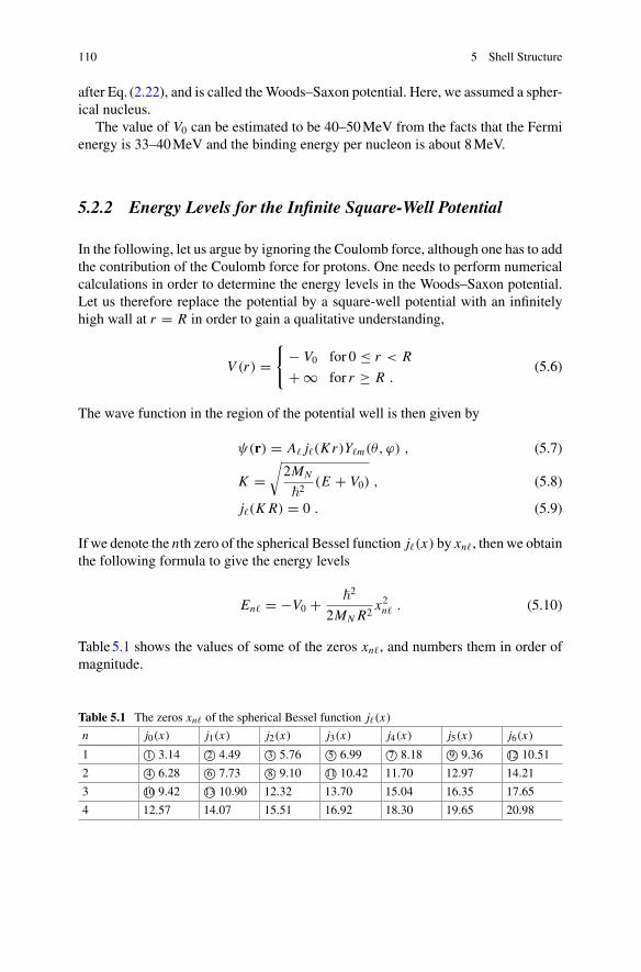
110 5 Shell Structure
after Eq. (2.22), and is called theWoods–Saxon potential. Here, we assumed a spher-ical nucleus.
The value of V0 can be estimated to be 40–50MeV from the facts that the Fermienergy is 33–40MeV and the binding energy per nucleon is about 8MeV.
5.2.2 Energy Levels for the Infinite Square-Well Potential
In the following, let us argue by ignoring the Coulomb force, although one has to addthe contribution of the Coulomb force for protons. One needs to perform numericalcalculations in order to determine the energy levels in the Woods–Saxon potential.Let us therefore replace the potential by a square-well potential with an infinitelyhigh wall at r = R in order to gain a qualitative understanding,
V (r) ={
− V0 for 0 ≤ r < R
+ ∞ for r ≥ R .(5.6)
The wave function in the region of the potential well is then given by
ψ(r) = A� j�(Kr)Y�m(θ, ϕ) , (5.7)
K =√2MN
�2(E + V0) , (5.8)
j�(K R) = 0 . (5.9)
If we denote the nth zero of the spherical Bessel function j�(x) by xn�, then we obtainthe following formula to give the energy levels
En� = −V0 + �2
2MN R2x2n� . (5.10)
Table5.1 shows the values of some of the zeros xn�, and numbers them in order ofmagnitude.
Table 5.1 The zeros xn� of the spherical Bessel function j�(x)
n j0(x) j1(x) j2(x) j3(x) j4(x) j5(x) j6(x)
1 1© 3.14 2© 4.49 3© 5.76 5© 6.99 7© 8.18 9© 9.36 12© 10.51
2 4© 6.28 6© 7.73 8© 9.10 11© 10.42 11.70 12.97 14.21
3 10© 9.42 13© 10.90 12.32 13.70 15.04 16.35 17.65
4 12.57 14.07 15.51 16.92 18.30 19.65 20.98
5.2 Explanation of the Magic Numbers by Mean-Field Theory 111
5.2.3 The Harmonic Oscillator Model
The harmonic oscillator model, where the mean field is assumed to be given by thefollowing formula, is often used as a more convenient method,
V (r) = 1
2MNω2r2 . (5.11)
In this case, the energy eigenvalues and the quantum numbers are given by
Enx ,ny ,nz = �ω
(N + 3
2
), (5.12)
N = nx + ny + nz , (5.13)
nx , ny, nz = 0, 1, 2, . . . , (5.14)
in the Cartesian coordinates, i.e., in the Descartes coordinates, and by
En�m = �ω
(N + 3
2
), (5.15)
N = 2(n − 1) + � , principal quantum number, (5.16)
n = 1, 2, 3, . . . , radial quantum number, (5.17)
� = 0, 1, . . . , azimuthal quantum number (orbital angular momentum),(5.18)
m = −�,−� + 1, . . . , � − 1, � , magnetic quantum number, (5.19)
in the spherical polar coordinates. n is the quantum number or index which showsthe numerical order of the states with the same angular momentum when they arecounted from the lowest energy state. nr ≡ n − 1 = 0, 1, 2, . . . is also often usedfor n. nr is the number of nodes of the radial wave function at positions other thanthe origin of the coordinate system, i.e., within the potential well.
The energy levels and the wave functions in the case of Cartesian coordinates canbe easily obtained by the series expansion method or by the method using the cre-ation and annihilation operators as is explained in the standard textbook of quantummechanics, and the wave function is given by
ψnx (x) = Nnx Hnx (αx) exp
(−1
2α2x2
), (5.20)
α = √MNω/� , (5.21)
112 5 Shell Structure
by using the Hermite polynomials Hn .2 Nnx = ( α√π2nx (nx )! )
1/2 is the normalizationconstant.
One can easily guess which kinds of angular momentum states are included ineach energy level when the polar coordinates are used by considering the parityand the degeneracy of each energy level, which can be easily determined in theCartesian coordinates, and the fact that the representations in terms of the Cartesiancoordinates and the polar coordinates can be transformed to each other using a unitarytransformation.
Exercise 5.1 Let us write the wave function in the polar coordinates as
ψnr �m(r) ≡ Rnr �(r)Ylm(r) = unr �(r)
rYlm(r) . (5.22)
Show that the normalized radial wave function unr � is then given by
unr �(r) =√2α
Γ (� + 32 )
[Γ (nr + � + 3
2 )
nr !
]1/2x�+1e− 1
2 x2F
(−nr ; � + 3
2; x2)
(5.23)
= √2α
[nr !
Γ (nr + � + 32 )
]1/2x�+1e− 1
2 x2L
(�+ 12 )
nr (x2) , (5.24)
where x = αr . F is the confluent hypergeometric function,
F
(−nr ; � + 3
2; z)
=nr∑k=0
(−1)k2k(nrk
)(2� + 1)!!
(2� + 2k + 1)!! zk , (5.25)
and L(�+ 1
2 )nr is the generalized Laguerre polynomial.
5.2.4 The Magic Numbers in the Static PotentialDue to Short Range Force
The first and second columns from the left in Fig. 5.1 give the single-particle energylevels together with the quantum numbers based on Eqs. (5.15) and (5.10), respec-tively. The magic numbers appear when one energy level is fully occupied and theenergy gap to the next energy level is large. If we denote the number of states in the
2The parameter b which is defined by b ≡ 1/α = √�/MNω is also often used and is called the
oscillator parameter. It gives a measure of the strength of the potential which confines nucleons andhas the dimension of length. It gives the extension of the 0s-state and the measure of the size ofclusters such as the α-cluster.
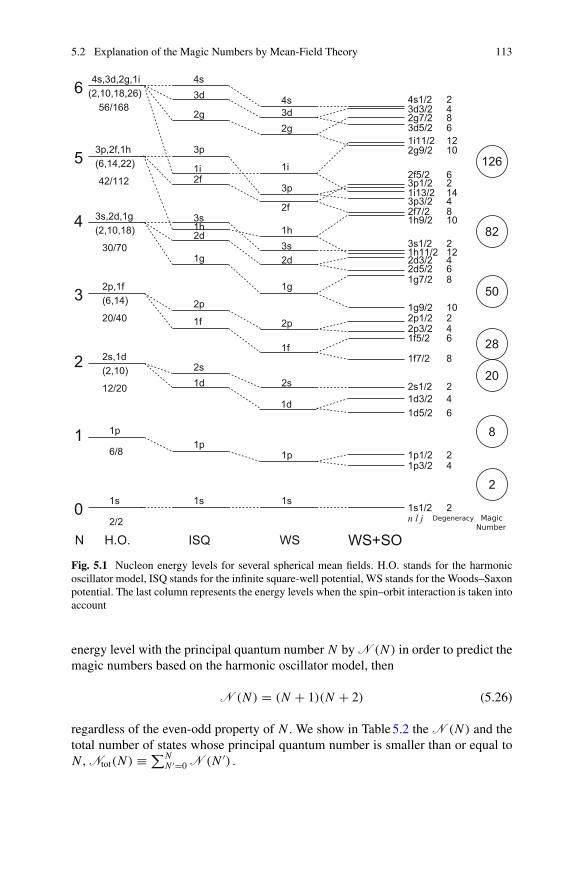
5.2 Explanation of the Magic Numbers by Mean-Field Theory 113
Fig. 5.1 Nucleon energy levels for several spherical mean fields. H.O. stands for the harmonicoscillator model, ISQ stands for the infinite square-well potential, WS stands for the Woods–Saxonpotential. The last column represents the energy levels when the spin–orbit interaction is taken intoaccount
energy level with the principal quantum number N byN (N ) in order to predict themagic numbers based on the harmonic oscillator model, then
N (N ) = (N + 1)(N + 2) (5.26)
regardless of the even-odd property of N . We show in Table5.2 the N (N ) and thetotal number of states whose principal quantum number is smaller than or equal toN ,Ntot(N ) ≡∑N
N ′=0 N (N ′) .
114 5 Shell Structure
Table 5.2 The degeneracy of energy levels and the magic numbers for the harmonic oscillatormodel
N 0 1 2 3 4 5 6 7
N (N ) 2 6 12 20 30 42 56 72
Ntot(N ) 2 8 20 40 70 112 168 240
Table5.2 shows that the magic numbers 2, 8 and 20 can be explained by theharmonic oscillator model. Figure5.1 shows that the infinite square-well potentialalso explains the small magic numbers 2, 8 and 20. In addition, in the square-wellpotential, the degeneracy concerning the angular momentum is resolved and the statewith larger angular momentum becomes energetically lower. This is because thestate with larger orbital angular momentum among the states with the same principalquantumnumber has larger probability in the surface region, and hencemore stronglyfeels the difference, i.e., a negative perturbation, between the square-well potentialand the harmonic oscillator potential.
The third column in Fig. 5.1 shows the energy levels for the Woods–Saxon poten-tial. The structure of the energy levels in this case resembles that for the square-wellpotential.
Exercise 5.2 Prove Eq. (5.26) by using thatN (N ) is given by∑N
�=0,2,...(2�+1)×2
when N is an even number and by∑N
�=1,3,...(2� + 1) × 2 when N is an odd numberbecause of the degeneracies concerning the magnetic quantum number and the spin.
5.2.5 Spin–Orbit Interaction
Suppose that the spin–orbit interaction is acting on each nucleon in addition tothe static central force in order to explain the magic numbers larger than 20. TheSchrödinger equation to determine the energy levels of nucleons is then given by
[− �
2
2MNΔ + V (r) + vLS(� · s)
]ψ(r) = Eψ(r) . (5.27)
We assume here that vLS = ξLS (constant) for simplicity.The modified energy levels for each N can be obtained by diagonalizing the
Hamiltonian with the degenerate states according to the perturbation theory fordegenerate case. Here, however, we use a more convenient method. Since the opera-tor �· s does not commute with any components of the orbital angular momentum andspin operator, their magnetic quantum numbers cannot be good quantum numbersseparately. On the other hand, since
[� · s, �2
]=[� · s, s2
]=[� · s, j2
]=[� · s, jα
]= 0 , (5.28)
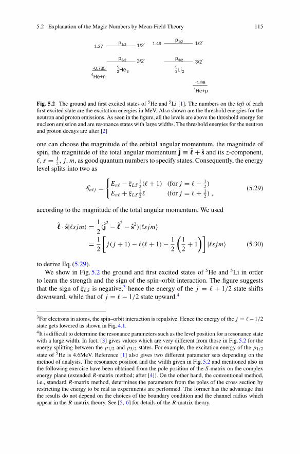
5.2 Explanation of the Magic Numbers by Mean-Field Theory 115
Fig. 5.2 The ground and first excited states of 5He and 5Li [1]. The numbers on the left of eachfirst excited state are the excitation energies in MeV. Also shown are the threshold energies for theneutron and proton emissions. As seen in the figure, all the levels are above the threshold energy fornucleon emission and are resonance states with large widths. The threshold energies for the neutronand proton decays are after [2]
one can choose the magnitude of the orbital angular momentum, the magnitude ofspin, the magnitude of the total angular momentum j ≡ � + s and its z-component,�, s = 1
2 , j,m, as good quantum numbers to specify states. Consequently, the energylevel splits into two as
En�j ={En� − ξLS
12 (� + 1) (for j = � − 1
2 )
En� + ξLS12� (for j = � + 1
2 ) ,(5.29)
according to the magnitude of the total angular momentum. We used
� · s|�s jm〉 = 1
2(j
2 − �2 − s2)|�s jm〉
= 1
2
[j ( j + 1) − �(� + 1) − 1
2
(1
2+ 1
)]|�s jm〉 (5.30)
to derive Eq. (5.29).We show in Fig. 5.2 the ground and first excited states of 5He and 5Li in order
to learn the strength and the sign of the spin–orbit interaction. The figure suggeststhat the sign of ξLS is negative,3 hence the energy of the j = � + 1/2 state shiftsdownward, while that of j = � − 1/2 state upward.4
3For electrons in atoms, the spin–orbit interaction is repulsive. Hence the energy of the j = �−1/2state gets lowered as shown in Fig. 4.1.4It is difficult to determine the resonance parameters such as the level position for a resonance statewith a large width. In fact, [3] gives values which are very different from those in Fig. 5.2 for theenergy splitting between the p1/2 and p3/2 states. For example, the excitation energy of the p1/2state of 5He is 4.6MeV. Reference [1] also gives two different parameter sets depending on themethod of analysis. The resonance position and the width given in Fig. 5.2 and mentioned also inthe following exercise have been obtained from the pole position of the S-matrix on the complexenergy plane (extended R-matrix method; after [4]). On the other hand, the conventional method,i.e., standard R-matrix method, determines the parameters from the poles of the cross section byrestricting the energy to be real as experiments are performed. The former has the advantage thatthe results do not depend on the choices of the boundary condition and the channel radius whichappear in the R-matrix theory. See [5, 6] for details of the R-matrix theory.
116 5 Shell Structure
Exercise 5.3 Estimate the magnitude of ξLS for protons and neutrons from Fig. 5.2.5
The width of the level is Γ = 648keV for the p3/2 state and Γ = 5.57MeV for thep1/2 state for 5He, while Γ = 1.23MeV for p3/2 state and Γ = 6.60MeV for p1/2state for 5Li [1]. Estimate the half-life and the mean life of the ground and excitedstates of 5He and 5Li from these values.
The last column of Fig. 5.1 gives the nucleon energy levels when the effect of thespin–orbit interaction is added based on these considerations. Each energy level isdesignated by the set of the radial quantum number n, the orbital angular momentum� and the total angularmomentum j . The figure shows that themagic numbers 28, 50,82, 126 arise due to the spin–orbit interaction.6 Note that there are 2 j +1 degeneratestates with different magnetic quantum numbers in a single energy level with theangular momentum j .
Note that the magic numbers 50, 82 and 126 are caused by the penetration of thej = � + 1/2 levels with a large orbital angular momentum into the energy regionof the energy levels with the principal quantum number N smaller by one due to thespin–orbit interaction and the surface effect, i.e., the effect that the realistic potentialis deeper in the surface region than that in the harmonic oscillator model. These statesare called intruder states. The 1g9/2, 1h11/2 and 1i13/2 levels play the principal roleas the intruder states for the magic numbers 50, 82 and 126, respectively.
Exercise 5.4 Answer the following questions concerning the transformation fromthe |� s = 1
2 m�ms〉 basis to the |�s jm j 〉 basis.1. Show that the total number of states is (2� + 1) × 2 in both bases.2. The states are given by |Y�mα〉 and |Y�mβ〉 in the former basis, where α and
β represent the spin-up and spin-down states, respectively. Write the generalexpression of theUnitary transformationwhich represents the |�s j = �+1/2 m j 〉and |�s j = � − 1/2 m j 〉 states in the |�sm�ms〉 basis. Also, write explicitly the| f7/2 m = 7/2〉 and | f5/2 m = 5/2〉 in terms of Y3m, α, β.
Sidebar: Japanese Contribution to the Development of Shell model—Pioneersof History: Tadayoshi Hikosaka and Takahiko Yamanouchi The independentparticle model, i.e., the shell model, thus succeeds in explaining the existence andthe actual numbers of magic numbers through the shell layer structure of the energylevels of nucleons, and the Pauli exclusion principle. Historically, pioneering studiesof the independent particle model (shell model) had been developed in Japan too byTadayoshi Hikosaka, Tohoku University, and Takahiko Yamanouchi, University ofTokyo. However, their pioneering works had been forgotten before their theory isaccepted as the correct effective model for many nuclear properties.
5It is necessary to handle both the ground and excited states as resonance states in order to achievea quantitatively accurate estimate. Here, however, use the harmonic oscillator model and ignore theradial dependence of the spin–orbit force in order to obtain a rough estimate of ξLS.6The tensor force also strongly affects the magic numbers and the shape of nucleus, and is one ofthe active research subjects in recent years in connection with, e.g., the structure of unstable nucleisuch as the change of the magic number. For example, 40Ca is spherical, but 32Mg is deformedamong the N = 20 isotones (see [7]).
5.2 Explanation of the Magic Numbers by Mean-Field Theory 117
There remain historical episodes that both Hikosaka and Yamanouchi receivedstrong objections when they discussed with Niels Bohr based on the success ofthe liquid-drop model to explain fission and the compound nucleus reactions. Onthe contrary, the existence of magic numbers was a strong experimental evidence inthe cases of Mayer and Jensen who established the shell model later. There remainsalso an episode that Jensen got the inspiration of the spin–orbit interaction while hewas attending a dance party. Incidentally, Hikosaka is the same person as who hasproposed the heterogeneous reactor.
Exercise 5.5 The puzzle of themagic numbers:Comparisonwith the cases for atomsand microclusters. Discuss the magic numbers for many-body systems of fermionswhen the interactions among the constituent particles can be approximated by themean fields listed below in the zeroth order approximation.
1. An attractive potential proportional to 1/r when the distance from the center isdenoted by r (periodic table of the elements).
2. Spherical Woods–Saxon potential (magic numbers for Alkali metals [8]).3. Three-dimensional harmonic oscillator plus attractive spin–orbit interaction
(magic numbers for nuclei).4. Three-dimensional harmonic oscillator plus repulsive spin–orbit interaction.5. Two-dimensional harmonic oscillator.
5.3 The Spin and Parity of the Ground and Low-LyingStates of Doubly-Magic ±1 Nuclei
The nucleus in which both proton and neutron numbers are magic numbers such as168O8 and 208
82 Pb126 is called doubly-magic nucleus or doubly-closed shell nucleus.One can predict the spin and parity of the ground state of the nuclei whose protonor neutron number is smaller or larger than those of a doubly-magic nucleus by oneby using the shell model. The spin and parity of low-lying states of those nuclei canalso be predicted to some extent.
Consider 20982 Pb for example. For the ground state, the single-particle energy levelsare successively filled with nucleons from the lowest energy level according to thePauli exclusion principle. Figure5.1 suggests that all the 82 protons are just filled inthe states from the n� j = 1s1/2 level to the 3s1/2 level. The 126 neutrons occupy allthe states from the 1s1/2 to the 2 f5/2 levels. Let us call this part, which correspondsto doubly-magic numbers, the core part. One then fills the last 127th neutron, calledthe valence neutron, in the next energy level 2g9/2. Since there is only one way to fillall the 2 j + 1 degenerate states for a given n� j with the same number of particles,Jtot =0 because of 2Jtot + 1 = 1 if we denote the total spin of these 2 j + 1 nucleonsby Jtot. Also, the total parity of these nucleons is plus irrespective of the even–oddproperty of the orbital angular momentum �, since 2 j + 1 is always an even number.Consequently, the total spin and parity of the nucleons forming the core are 0+. As
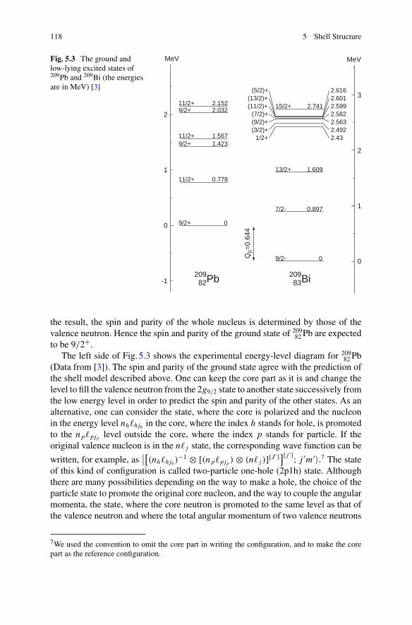
118 5 Shell Structure
Fig. 5.3 The ground andlow-lying excited states of209Pb and 209Bi (the energiesare in MeV) [3]
the result, the spin and parity of the whole nucleus is determined by those of thevalence neutron. Hence the spin and parity of the ground state of 209
82 Pb are expectedto be 9/2+.
The left side of Fig. 5.3 shows the experimental energy-level diagram for 20982 Pb
(Data from [3]). The spin and parity of the ground state agree with the prediction ofthe shell model described above. One can keep the core part as it is and change thelevel to fill the valence neutron from the 2g9/2 state to another state successively fromthe low energy level in order to predict the spin and parity of the other states. As analternative, one can consider the state, where the core is polarized and the nucleonin the energy level nh�h jh in the core, where the index h stands for hole, is promotedto the np�pjp level outside the core, where the index p stands for particle. If theoriginal valence nucleon is in the n� j state, the corresponding wave function can be
written, for example, as∣∣[(nh�h jh )−1 ⊗ [(np�pjp ) ⊗ (n� j )][J ′]][ j ′]; j ′m ′〉.7 The state
of this kind of configuration is called two-particle one-hole (2p1h) state. Althoughthere are many possibilities depending on the way to make a hole, the choice of theparticle state to promote the original core nucleon, and the way to couple the angularmomenta, the state, where the core neutron is promoted to the same level as that ofthe valence neutron and where the total angular momentum of two valence neutrons
7We used the convention to omit the core part in writing the configuration, and to make the corepart as the reference configuration.
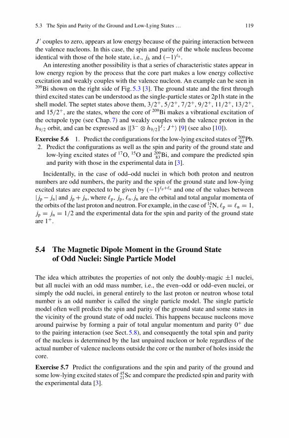
5.3 The Spin and Parity of the Ground and Low-Lying States … 119
J ′ couples to zero, appears at low energy because of the pairing interaction betweenthe valence nucleons. In this case, the spin and parity of the whole nucleus becomeidentical with those of the hole state, i.e., jh and (−1)�h .
An interesting another possibility is that a series of characteristic states appear inlow energy region by the process that the core part makes a low energy collectiveexcitation and weakly couples with the valence nucleon. An example can be seen in209Bi shown on the right side of Fig. 5.3 [3]. The ground state and the first throughthird excited states can be understood as the single-particle states or 2p1h state in theshell model. The septet states above them, 3/2+, 5/2+, 7/2+, 9/2+, 11/2+, 13/2+,and 15/2+, are the states, where the core of 209Bi makes a vibrational excitation ofthe octupole type (see Chap.7) and weakly couples with the valence proton in theh9/2 orbit, and can be expressed as |[3− ⊗ h9/2]J ; J+〉 [9] (see also [10]).
Exercise 5.6 1. Predict the configurations for the low-lying excited states of 20982 Pb.2. Predict the configurations as well as the spin and parity of the ground state and
low-lying excited states of 17O, 15O and 20983Bi, and compare the predicted spin
and parity with those in the experimental data in [3].
Incidentally, in the case of odd–odd nuclei in which both proton and neutronnumbers are odd numbers, the parity and the spin of the ground state and low-lyingexcited states are expected to be given by (−1)�p+�n and one of the values between| jp − jn| and jp + jn, where �p, jp, �n. jn are the orbital and total angular momenta ofthe orbits of the last proton and neutron. For example, in the case of 147N, �p = �n = 1,jp = jn = 1/2 and the experimental data for the spin and parity of the ground stateare 1+.
5.4 The Magnetic Dipole Moment in the Ground Stateof Odd Nuclei: Single Particle Model
The idea which attributes the properties of not only the doubly-magic ±1 nuclei,but all nuclei with an odd mass number, i.e., the even–odd or odd–even nuclei, orsimply the odd nuclei, in general entirely to the last proton or neutron whose totalnumber is an odd number is called the single particle model. The single particlemodel often well predicts the spin and parity of the ground state and some states inthe vicinity of the ground state of odd nuclei. This happens because nucleons movearound pairwise by forming a pair of total angular momentum and parity 0+ dueto the pairing interaction (see Sect. 5.8), and consequently the total spin and parityof the nucleus is determined by the last unpaired nucleon or hole regardless of theactual number of valence nucleons outside the core or the number of holes inside thecore.
Exercise 5.7 Predict the configurations and the spin and parity of the ground andsome low-lying excited states of 4521Sc and compare the predicted spin and parity withthe experimental data [3].
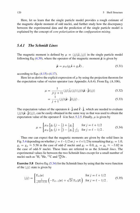
120 5 Shell Structure
Here, let us learn that the single particle model provides a rough estimate ofthe magnetic dipole moment of odd nuclei, and further study how the discrepancybetween the experimental data and the prediction of the single particle model isexplained by the concept of core polarization or the configuration mixing.
5.4.1 The Schmidt Lines
The magnetic moment is defined by μ ≡ 〈 j j |μz| j j〉 in the single particle modelfollowing Eq. (4.39), where the operator of the magnetic moment μ is given by
μ = μN (gs s + g��) , (5.31)
according to Eqs. (4.15)–(4.17).Here let us derive the explicit expression of μ by using the projection theorem for
the expectation value of vector operator (see Appendix A.6.4). From Eq. (A.106),
μ = 1
j ( j + 1)〈 j j | jZ | j j〉〈 j j |(μ · j)| j j〉 (5.32)
= 1
j + 1〈 j j |(μ · j)| j j〉 . (5.33)
The expectation values of the operators s · j and � · j , which are needed to evaluate〈 j j |(μ · j)| j j〉, can be easily obtained in the same way as that was used to obtain theexpectation value of the operator � · s in Sect. 5.2.5. Finally, μ is given by
μ ={
μN[g�
(j − 1
2
)+ 12gs]
for j = � + 1/2
μN[g�
(j + 3
2
)− 12gs] j
j+1 for j = � − 1/2 .(5.34)
Thus one can expect that the magnetic moments are given by the solid lines inFig. 5.4 depending onwhether j = �−1/2 or j = �+1/2 by remarking that g� = 1.0,gs = gp ≈ 5.58 in the case of odd-Z nuclei and g� = 0.0, gs = gn ≈ −3.82 inthe case of odd-N nuclei. These lines are referred to as the Schmidt lines. Theexperimental values lie between the two Schmidt lines except for a small number ofnuclei such as 3H, 3He, 13C and 189
76Os .
Exercise 5.8 Derive Eq. (5.34) for the Schmidt lines by using that the wave functionof the | j j〉 state is given by
| j j〉 ={Y��|α〉 for j = � + 1/2
1√2(�+1/2)
(−Y��−1|α〉 + √
2� Y��|β〉)
for j = � − 1/2 .(5.35)
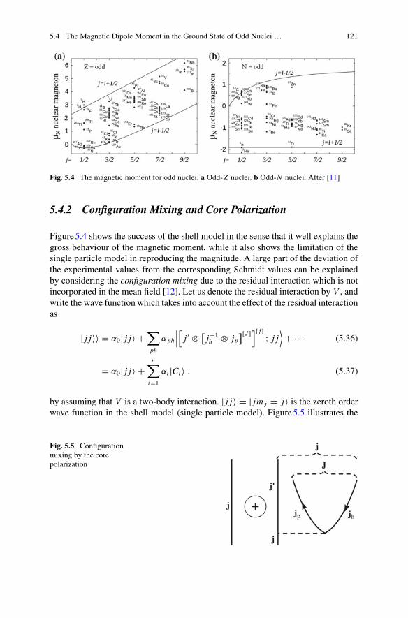
5.4 The Magnetic Dipole Moment in the Ground State of Odd Nuclei … 121
Fig. 5.4 The magnetic moment for odd nuclei. a Odd-Z nuclei. b Odd-N nuclei. After [11]
5.4.2 Configuration Mixing and Core Polarization
Figure5.4 shows the success of the shell model in the sense that it well explains thegross behaviour of the magnetic moment, while it also shows the limitation of thesingle particle model in reproducing the magnitude. A large part of the deviation ofthe experimental values from the corresponding Schmidt values can be explainedby considering the configuration mixing due to the residual interaction which is notincorporated in the mean field [12]. Let us denote the residual interaction by V , andwrite the wave function which takes into account the effect of the residual interactionas
| j j〉〉 = α0| j j〉 +∑ph
αph
∣∣∣[ j ′ ⊗ [ j−1h ⊗ jp
][J ]][ j] ; j j⟩+ · · · (5.36)
= α0| j j〉 +n∑
i=1
αi |Ci 〉 . (5.37)
by assuming that V is a two-body interaction. | j j〉 = | jm j = j〉 is the zeroth orderwave function in the shell model (single particle model). Figure5.5 illustrates the
Fig. 5.5 Configurationmixing by the corepolarization
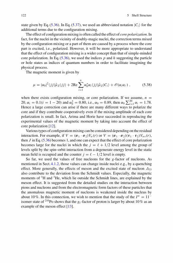
122 5 Shell Structure
state given by Eq. (5.36). In Eq. (5.37), we used an abbreviated notation |Ci 〉 for theadditional terms due to the configuration mixing.
The effect of configurationmixing is often called the effect of core polarization. Infact, for the nuclei in the vicinity of doubly-magic nuclei, the correction terms mixedby the configuration mixing or a part of them are caused by a process where the corepart is excited, i.e., polarized. However, it will be more appropriate to understandthat the effect of configuration mixing is a wider concept than that of simple-mindedcore polarization. In Eq. (5.36), we used the indices p and h suggesting the particleor hole states as indices of quantum numbers in order to facilitate imagining thephysical process.
The magnetic moment is given by
μ = |α0|2〈 j j |μZ | j j〉 + 2Ren∑
i=1
α∗0αi 〈 j j |μZ |Ci 〉 + O(αiαi ′) , (5.38)
when there exists configuration mixing, or core polarization. If we assume, n =20, αi = 0.1(i = 1 − 20) and α2
0 = 0.80, i.e., α0 = 0.89, then α0∑20
i=1 αi = 1.78.Hence a large correction can arise if there are many different ways to polarize thecore and if they contribute cooperatively even if the mixing amplitude of each corepolarization is small. In fact, Arima and Horie have succeeded in reproducing theexperimental values of the magnetic moment by taking into account the effect ofcore polarization [12].
Various types of configurationmixing can be considered depending on the residualinteraction. For example, if V = (σ 1 · σ 2)Vσ (r) or V = (σ 1 · σ 2)(τ 1 · τ 2)Vστ (r),then J in Eq. (5.36) becomes 1, and one can expect that the effect of core polarizationbecomes large for the nuclei in which the j = � + 1/2 level among the group oflevels split by the spin–orbit interaction from a degenerate energy level in the staticmean field is occupied and the counter j = � − 1/2 level is empty.
So far, we used the values of free nucleons for the g-factor of nucleons. Asmentioned in Sect. 4.1.2, those values can change inside nuclei e.g., by a quenchingeffect. More generally, the effects of meson and the excited state of nucleon Δ33
also contribute to the deviation from the Schmidt values. Especially, the magneticmoments of 3H and 3He, which lie outside the Schmidt lines, are explained by themeson effect. It is suggested from the detailed studies on the interaction betweenpions and nucleons and from the electromagnetic form factors of these particles thatthe anomalous magnetic moment of nucleons is weakened inside the nucleus byabout 10%. In this connection, we wish to mention that the study of the I π = 11−isomer state of 210Po shows that the g�-factor of proton is larger by about 10% as anexample of the meson effect [13].
5.4 The Magnetic Dipole Moment in the Ground State of Odd Nuclei … 123
5.4.3 [Addendum] The Anomalous Magnetic Momentsof Nucleons in the Quark Model
In Chap.1, we attributed the anomalous magnetic moments of nucleons to the effectsof meson cloud. Alternatively, here we show that the anomalous magnetic momentsof nucleons can be naturally derived from the point of view of the quark model.
In the quark model, proton is made up of two u quarks and one d quark. It isconsidered that all the baryons existing in nature are in the color-singlet state, whichis antisymmetric concerning the color degree of freedom, and are spatially symmetricin low-energy states. Hence the wave function for proton in the combined spaces ofthe spin and flavor degrees of freedom must be symmetric in total, and is given by[14]
|p ↑〉 =√
1
18
[uud(↑↓↑ + ↓↑↑ −2 ↑↑↓) + udu(↑↑↓ + ↓↑↑ −2 ↑↓↑)
+ duu(↑↓↑ + ↑↑↓ −2 ↓↑↑)]
. (5.39)
Similarly, the wave function for |n ↑〉 state is given by interchanging u and d quarks.On the other hand, the operator of the magnetic moment of the i th quark is given
by
μ(q)i = Q(q)
i
e�
2m(q)i c
σ(q)i ≡ μi σ
(q)i (5.40)
if we assume that quarks are structureless Dirac particles, where Q(q)i e and m(q)
i arethe charge and the mass of the i th quark. The magnetic dipole moment of proton isgiven by
μp =3∑
i=1
〈p ↑ |μ(q)i z |p ↑〉 , (5.41)
following the definition (4.39). Using Eq. (5.39) in Eq. (5.41), we obtain
μp = 1
3(4μu − μd) . (5.42)
Similarly, we obtainμn = 1
3(4μd − μu) (5.43)
for themagnetic dipole moment of neutron. If we identify the quarks with constituentquarks and assume that mu = md, then it follows
μn
μp= −2
3. (5.44)
This value well agrees with the experimental value μn/μp ≈ −0.685.
124 5 Shell Structure
Exercise 5.9 Estimate the value of μp by assuming muc2 = mdc2 ≈ 300MeV, andcompare the estimated value with the experimental data.
5.5 Mass Number Dependence of the Level Spacing �ω
The spacing between two successive energy levels, i.e., �ω in the harmonic oscillatormodel, plays the central role in the shell model. Here, we estimate the value of �ω.
We learnt in Sect. 2.1 that the mean-square radius for stable nuclei is given by
〈r2〉 = 3
5R2eq = 3
5r20 A
2/3 (5.45)
by using a radius parameter r0 ∼ 1.2 fm and the mass number A.We have
〈r2〉 ≡ 1
A
A∑k=1
〈r2k 〉 (5.46)
= 1
A
Nmax∑N=0
�
MNω
(N + 3
2
)(N + 1)(N + 2) × 2 (5.47)
≈ 1
A
�
MNω
1
2(Nmax + 2)4 (5.48)
from the definition of the mean-square radius. We used the following virial theorem,
1
2MNω2〈r2〉N = 〈V 〉N = 1
2EN = 1
2�ω
(N + 3
2
), (5.49)
to transform from Eq. (5.46) to (5.47).On the other hand, we have
A =Nmax∑N=0
(N + 1)(N + 2) × 2 ≈ 2
3(Nmax + 2)3 . (5.50)
We assumed Nmax + 2 � 1 in deriving Eqs. (5.48) and (5.50). Equations (5.48) and(5.50) lead to
〈r2〉 = 1
2
(3
2
)4/3�
MNωA1/3 . (5.51)
5.5 Mass Number Dependence of the Level Spacing �ω 125
Thus we obtain
�ω = 1
2
(3
2
)4/3(�c)2
MNc25
3r−20 A−1/3 ∼ 41.1A−1/3 MeV (5.52)
from Eq. (5.45).
5.6 The Magnitude and Origin of Spin–Orbit Interaction
It will beworth commenting on themagnitude and origin of the spin–orbit interaction[15]. For nuclei with large mass numbers, the spin–orbit interaction is suggested tobe
VLS ∼ −20� · sA−2/3 MeV (5.53)
from the experimental data for the energy difference between the j = � + 1/2and j = � − 1/2 states split by the spin–orbit interaction. Since � ∼ kF R =(9π/8)1/3A1/3 for nucleons in the vicinity of the Fermi surface, VLS becomes non-negligible compared with �ω given by Eq. (5.52), and plays an important role indetermining magic numbers.
The spin–orbit interaction used inEq. (5.27) is the one-body spin–orbit interaction.It originates partly from the two-body spin–orbit interaction, which we studied inSect. 3.2.2, by averaging over the coordinates of one of the nucleons. The tensorforce is another source of the one-body spin–orbit interaction. In the relativisticmean-field theory which we learn in Sect. 6.3, the spin–orbit interaction originatesfrom the coupling of nucleons to the σ -, ρ-, ω-mesons, and depends on the isospinof nucleons due to the contribution of the ρ-meson.
5.7 Difference Between the Potentials for Protonsand for Neutrons: Lane Potential
The potential given by Eq. (5.1) corresponds to the Hartree potential which we learnin Sect. 6.1. More precisely, the strength of the potential V0 depends on the isospinof nucleons reflecting, e.g., the exchange effects, and is replaced by
V = V0 − 1
2tzN − Z
AV1 , (5.54)
if we take the definition that tz|n〉 = 12 |n〉, and tz|p〉 = − 1
2 |p〉. Hence the potential fornucleons depends on the isospin of nucleons. The isospin dependent term is calledthe Lane potential. One can estimate the strength of V1 as
126 5 Shell Structure
V1 ∼ 4b(pot)sym = 4
(bsym − b(kin)
sym
)≈ 100MeV
from themagnitude of the contribution of the potential energy to the symmetry energyterm in the mass formula.
Exercise 5.10 Show that
E (pot)sym ≈ 1
8
(N − Z)2
AV1 (5.55)
if we express the magnitude of the potential energy given by the Lane potential asE (pot)sym , hence that V1 ∼ 4b(pot)
sym .
The Lane potential can be derived in the following way. Suppose that the interac-tion between two nucleons is given by
V (x1, x2) = −V0(w + mPM)v(r1 − r2) = −V0(w + mPM)v(r12) (5.56)
= −V0
[w − m
1
4(1 + τ 1 · τ 2)(1 + σ 1 · σ 2)
]v(r12) , (5.57)
where PM is the Majorana operator, and w and m are the strength parameters of theWigner and Majorana forces, respectively. By ignoring the correlation between thenucleons, and adding on average with respect to the second nucleon, we obtain
V (r1) = −V0
(w − m
4
) [1 − m
w − m4
1
A(t · T)
]V (r1) , (5.58)
V (r1) ≡∫
ρ(r2)v(r12)dr2 , (5.59)
for the nucleon potential. T represents the total isospin operator of nucleons excludingthe nucleon under consideration. The isospin dependent term is nothing but the Lanepotential. Let us consider two cases in order to estimate the magnitude. One ofthe cases is the Serber exchange potential, where m = w = 1/2. In this case,w − m/4 = 3/8, m/(w − m/4) = 4/3. The other case is the Volkov force, whichis often used for the study of cluster structure of light nuclei. In this case, m = 0.6,w = 1 − m = 0.4. Hence w − m/4 = 0.25, m/(w − m/4) = 2.4. Since V0 and V1
in Eq. (5.54) are about 40 and 100MeV, respectively, the Volkov force well agreeswith the phenomenological strength of the Lane potential.
Physically, the Lane potential can be considered to reflect the fact that the forcebetween proton and neutron is stronger than the forces between protons and betweenneutrons. Since the difference is intimately related to the effect of the tensor force,one can suppose that the Volkov interaction is a force which effectively incorporatesthe effect of the tensor force.
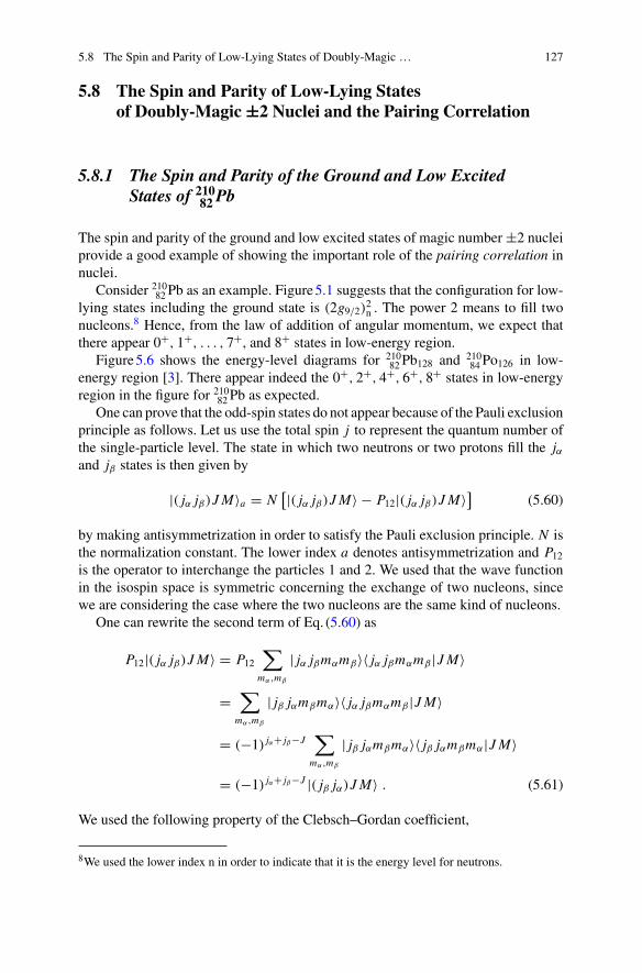
5.8 The Spin and Parity of Low-Lying States of Doubly-Magic … 127
5.8 The Spin and Parity of Low-Lying Statesof Doubly-Magic ±2 Nuclei and the Pairing Correlation
5.8.1 The Spin and Parity of the Ground and Low ExcitedStates of 21082Pb
The spin and parity of the ground and low excited states of magic number ±2 nucleiprovide a good example of showing the important role of the pairing correlation innuclei.
Consider 21082 Pb as an example. Figure5.1 suggests that the configuration for low-
lying states including the ground state is (2g9/2)2n . The power 2 means to fill twonucleons.8 Hence, from the law of addition of angular momentum, we expect thatthere appear 0+, 1+, . . . , 7+, and 8+ states in low-energy region.
Figure5.6 shows the energy-level diagrams for 21082 Pb128 and 210
84 Po126 in low-energy region [3]. There appear indeed the 0+, 2+, 4+, 6+, 8+ states in low-energyregion in the figure for 210
82 Pb as expected.One can prove that the odd-spin states do not appear because of the Pauli exclusion
principle as follows. Let us use the total spin j to represent the quantum number ofthe single-particle level. The state in which two neutrons or two protons fill the jαand jβ states is then given by
|( jα jβ)JM〉a = N[|( jα jβ)JM〉 − P12|( jα jβ)JM〉] (5.60)
by making antisymmetrization in order to satisfy the Pauli exclusion principle. N isthe normalization constant. The lower index a denotes antisymmetrization and P12is the operator to interchange the particles 1 and 2. We used that the wave functionin the isospin space is symmetric concerning the exchange of two nucleons, sincewe are considering the case where the two nucleons are the same kind of nucleons.
One can rewrite the second term of Eq. (5.60) as
P12|( jα jβ)JM〉 = P12∑mα,mβ
| jα jβmαmβ〉〈 jα jβmαmβ |JM〉
=∑mα,mβ
| jβ jαmβmα〉〈 jα jβmαmβ |JM〉
= (−1) jα+ jβ−J∑mα,mβ
| jβ jαmβmα〉〈 jβ jαmβmα|JM〉
= (−1) jα+ jβ−J |( jβ jα)JM〉 . (5.61)
We used the following property of the Clebsch–Gordan coefficient,
8We used the lower index n in order to indicate that it is the energy level for neutrons.
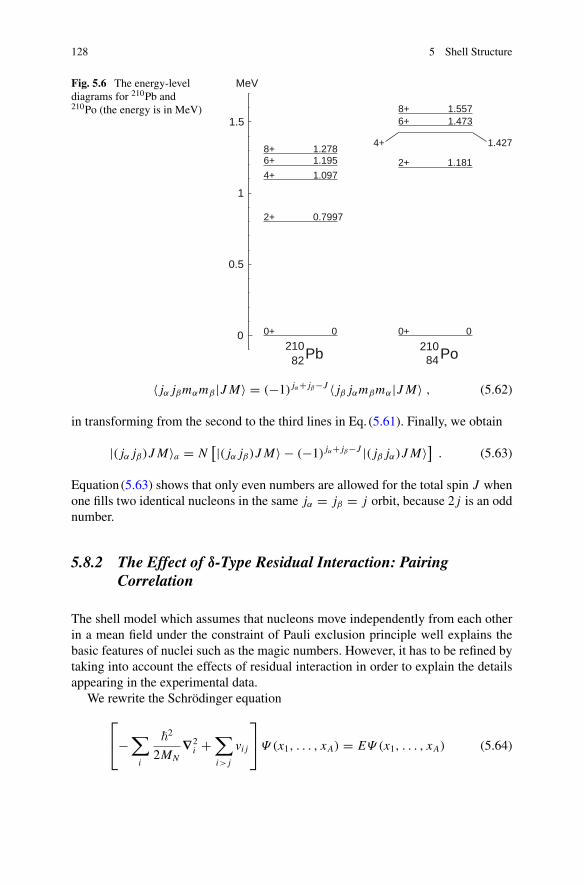
128 5 Shell Structure
Fig. 5.6 The energy-leveldiagrams for 210Pb and210Po (the energy is in MeV)
〈 jα jβmαmβ |JM〉 = (−1) jα+ jβ−J 〈 jβ jαmβmα|JM〉 , (5.62)
in transforming from the second to the third lines in Eq. (5.61). Finally, we obtain
|( jα jβ)JM〉a = N[|( jα jβ)JM〉 − (−1) jα+ jβ−J |( jβ jα)JM〉] . (5.63)
Equation (5.63) shows that only even numbers are allowed for the total spin J whenone fills two identical nucleons in the same jα = jβ = j orbit, because 2 j is an oddnumber.
5.8.2 The Effect of δ-Type Residual Interaction: PairingCorrelation
The shell model which assumes that nucleons move independently from each otherin a mean field under the constraint of Pauli exclusion principle well explains thebasic features of nuclei such as the magic numbers. However, it has to be refined bytaking into account the effects of residual interaction in order to explain the detailsappearing in the experimental data.
We rewrite the Schrödinger equation
⎡⎣−
∑i
�2
2MN∇2
i +∑i> j
vi j
⎤⎦Ψ (x1, . . . , xA) = EΨ (x1, . . . , xA) (5.64)
5.8 The Spin and Parity of Low-Lying States of Doubly-Magic … 129
for an A-nucleon system, where the nucleons are interacting with each other throughthe two-body interaction v, into
⎧⎨⎩∑i
[− �
2
2MN∇2
i +U (xi )
]+∑i> j
Vi j
⎫⎬⎭Ψ (x1, . . . , xA) = EΨ (x1, . . . , xA)
(5.65)by introducing a mean field U (x). V is the residual interaction if we consider theh(0) ≡ −�
2∇2/2MN +U as the unperturbed single-particle Hamiltonian of the shellmodel which uses, e.g., the harmonic oscillator potential for U .
We learnt in Sect. 5.4.2 that the residual interaction plays an important role in themagnetic moment. The degenerate 0+, 2+, . . . , 8+ levels in 210
82 Pb are also resolvedby the residual interaction.
Let us assume that the residual interaction between two nucleons is given by
V (r1 − r2) = −V0δ(r1 − r2) . (5.66)
Using the perturbation theory, one can then show (see Appendix A.11) that theenergy of two-nucleon system, where each of the single-particle levels (nα�α jα) and(nβ�β jβ) is occupied by one nucleon and their angular momenta couple to the totalangular momentum J , changes by the amount of
ΔEJ = −V0
2
[1 + (−1)�α+�β−J
]F(nα�α, nβ�β)A( jα jβ; J ) , (5.67)
where
F(nα�α, nβ�β) =∫ ∞
0
1
r2u2nα�α
(r)u2nβ�β(r)dr , (5.68)
A( jα jβ; J ) = 1
1 + δnαnβδ�α�β
δ jα jβ
1
4π
(2 jα + 1)(2 jβ + 1)
2J + 1
⟨jα jβ
1
2− 1
2
∣∣∣∣ J0⟩2
,
(5.69)
where un�(r) is the radial wave function defined according to Eq. (5.22). Equa-tions (5.67)–(5.69) show that the energy shift by the residual interaction dependson the total spin J only through the factor A via the Clebsch–Gordan coefficient and2J + 1. Table5.3 shows the factor A as a function of J for the case when we filltwo identical nucleons in the same jα = jβ = 9/2 orbit. The table suggests thatthe energy split among the 0+, 2+, . . . , 8+ states shown in Fig. 5.6 has been inducedby the short-range residual interaction of δ-function type. The J = 0 state appearsas the lowest energy level, because in that state two nucleons move in the sameorbit with opposite directions, so that the spatial overlap is large. Consequently, thecorrelation energy of attractive δ-function type is maximized. The spatial overlap oftwo nucleons gets smaller with increasing J . Accordingly the energy shift from theenergy in the independent particle model becomes smaller. Note that the energy shift
130 5 Shell Structure
Table 5.3 The angular momentum dependence of the energy shift factor A for the case of jα =jβ = 9/2
J 0 2 4 6 8
8π A 10 80/33 (2.42) 180/143 (1.26) 320/429 (0.75) 980/2439 (0.40)
for the J = 0 state is especially large, and that the interval between the successiveenergy levels gets narrower with increasing J . The J dependence shown in Table5.3can be qualitatively understood from the following asymptotic formula which holdswhen both j and J are large [16],
⟨j j1
2− 1
2
∣∣∣∣ J0⟩2
∼ 2
π
1
j + 12
√4 j ( j + 1)
(2 j + 1)2(J + 1
2 )2
J (J + 1)− (J + 1
2 )2
(2 j + 1)2
∼ 2
π j
√1 −
(J
2 j
)2
. (5.70)
In this way, in the ground state of nuclei, two identical nucleons occupy two orbits,which are time-reversed orbits to each other, as a pair of the total angular momentumJ = 0. This is called the pairing correlation in nuclei and corresponds to theCooperpair and superfluidity in condensed matter physics.9
5.9 Column: Superheavy Elements (SHE)
As stated in Sect. 2.3.4 concerning the stability with respect to fission, the liquid-drop modelsuggests that thefission barrier disappearswhen the atomic number exceeds about 100, becausethe Coulomb force which prefers to fission then overcomes the surface tension which resistsfission.Hence it predicts that there exist noheavynuclei beyond Z ∼ 100.However, theoreticalcalculations predict that there appear fission barriers due to shell effect and that the atomicnumber Z = 114 and the neutron number N = 18410 are the magic numbers next to theknown magic numbers Z = 82 and N = 126 and that there exists a region of relatively stablenuclei around the set of these numbers in the nuclear chart. They are called superheavy nucleiand the corresponding elements are called superheavy elements (SHE). Extensive activitiesto examine such theoretical prediction and to explore the limit of existence of nuclei in theregion of large mass number are continued.
Figures5.7 and 5.8 show reports of the Joint Institute for Nuclear Research (JINR) inDubna, Russia and the RIKEN at Wako, Japan, which are currently the world centers ofexperimental activities in this subject. In Fig. 5.7, the superheavy nuclei synthesized by theso-called hot fusion which uses actinides such as Cf and Cm as the target and 48Ca as theprojectile are shown by circles and the superheavy nuclei synthesized by the cold fusionwhich
9One can rigorously discuss the level structure in the presence of the pairing correlation in analgebraic way by using the quasi-spin formalism if one simplifies that only the pair whose totalangular momentum J is zero is affected by the attractive residual interaction [17].10These numbers vary somewhat depending on the theoretical models.
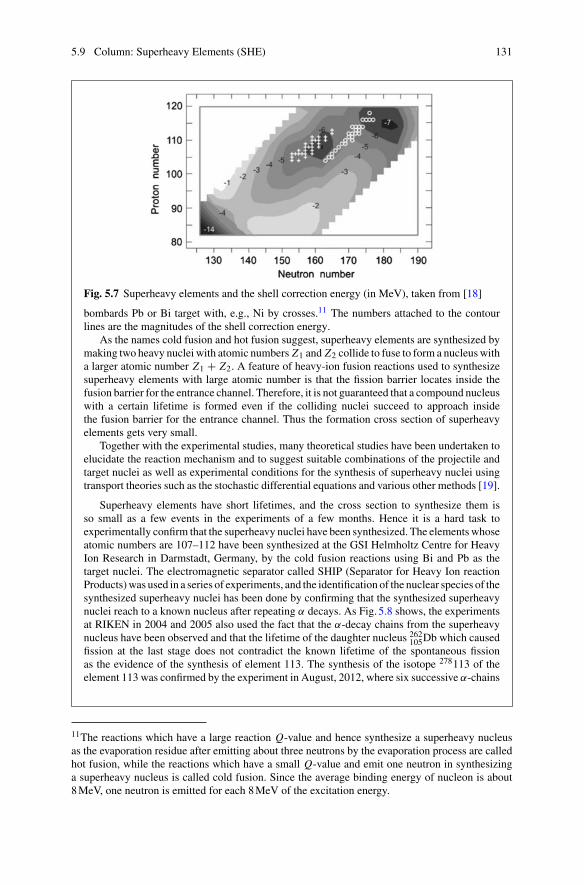
5.9 Column: Superheavy Elements (SHE) 131
Fig. 5.7 Superheavy elements and the shell correction energy (in MeV), taken from [18]
bombards Pb or Bi target with, e.g., Ni by crosses.11 The numbers attached to the contourlines are the magnitudes of the shell correction energy.
As the names cold fusion and hot fusion suggest, superheavy elements are synthesized bymaking two heavy nuclei with atomic numbers Z1 and Z2 collide to fuse to form a nucleuswitha larger atomic number Z1 + Z2. A feature of heavy-ion fusion reactions used to synthesizesuperheavy elements with large atomic number is that the fission barrier locates inside thefusion barrier for the entrance channel. Therefore, it is not guaranteed that a compound nucleuswith a certain lifetime is formed even if the colliding nuclei succeed to approach insidethe fusion barrier for the entrance channel. Thus the formation cross section of superheavyelements gets very small.
Together with the experimental studies, many theoretical studies have been undertaken toelucidate the reaction mechanism and to suggest suitable combinations of the projectile andtarget nuclei as well as experimental conditions for the synthesis of superheavy nuclei usingtransport theories such as the stochastic differential equations and various other methods [19].
Superheavy elements have short lifetimes, and the cross section to synthesize them isso small as a few events in the experiments of a few months. Hence it is a hard task toexperimentally confirm that the superheavy nuclei have been synthesized. The elementswhoseatomic numbers are 107–112 have been synthesized at the GSI Helmholtz Centre for HeavyIon Research in Darmstadt, Germany, by the cold fusion reactions using Bi and Pb as thetarget nuclei. The electromagnetic separator called SHIP (Separator for Heavy Ion reactionProducts)was used in a series of experiments, and the identification of the nuclear species of thesynthesized superheavy nuclei has been done by confirming that the synthesized superheavynuclei reach to a known nucleus after repeating α decays. As Fig. 5.8 shows, the experimentsat RIKEN in 2004 and 2005 also used the fact that the α-decay chains from the superheavynucleus have been observed and that the lifetime of the daughter nucleus 262
105Db which causedfission at the last stage does not contradict the known lifetime of the spontaneous fissionas the evidence of the synthesis of element 113. The synthesis of the isotope 278113 of theelement 113 was confirmed by the experiment in August, 2012, where six successive α-chains
11The reactions which have a large reaction Q-value and hence synthesize a superheavy nucleusas the evaporation residue after emitting about three neutrons by the evaporation process are calledhot fusion, while the reactions which have a small Q-value and emit one neutron in synthesizinga superheavy nucleus is called cold fusion. Since the average binding energy of nucleon is about8MeV, one neutron is emitted for each 8MeV of the excitation energy.
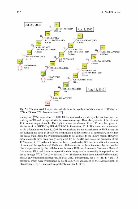
132 5 Shell Structure
Fig. 5.8 The observed decay chains which show the synthesis of the element 278113 by the209Bi+ 70Zn→ 278113+n reactions [20]
leading to 254101Md were observed [20]. Of the observed six α-decays the last two, i.e., the
α-decays of Db and Lr, agreed with the known α-decays. Thus, the synthesis of the element113 became unquestionable. The right to name the element Z = 113 was then given toMorita et al. at RIKEN by IUPAP/IUPAC in December, 2015. The name was announcedas Nh (Nihonium) on June 8, 2016. By comparison, for the experiments at JINR using thehot fusion it has been an obstacle to confirmation of the synthesis of superheavy nuclei thatthe decay chains from the synthesized nuclei do not connect to the known region. However,those elements have been finally recognized by IUPAP/IUPAC, since the synthesis of the112th element (283Cn) by hot fusion has been reproduced at GSI, and in addition the numberof events of the synthesis of 114th and 116th elements has been increased by the double-check experiments by the collaboration between JINR and Lawrence Livermore NationalLaboratory, USA and it was accepted that their decay can be reasonably interpreted as thedecay through 283Cn. The Z = 114 and Z = 116 elements have been named Fl (Flerovium)and Lv (Livermorium), respectively, in May, 2012. Furthermore, the Z = 115, 117 and 118elements, which were synthesized by hot fusion, were announced as Mc (Moscovium), Ts(Tennessine), Og (Oganesson), respectively, on June 8, 2016.
References 133
References
1. D.R. Tilley et al., Nucl. Phys. A 708, 3 (2002)2. National Nuclear Data Center. http://www.nndc.bnl.gov/nudat2/3. C.M. Lederer, V. Shirley, Table of Isotopes, 7th edn. (Wiley, New York, 1978)4. A. Csótó, G.M. Hale, Phys. Rev. C 55, 536 (1997)5. M.A. Preston, Physics of the Nucleus (Addison-Wesley, London, 1962)6. A.M. Lane, R.G. Thomas, Rev. Mod. Phys. 30, 257 (1958)7. T. Otsuka, T. Suzuki, R. Fujimoto, H. Grawe, Y. Akaishi, Phys. Rev. Lett. 95, 232502 (2005)8. W.D. Knight et al., Phys. Rev. Lett. 52, 2141 (1984)9. I. Hamamoto, Nucl. Phys. A 126, 545 (1969); 141, 1 (1970); 155, 362 (1970)10. A. Bohr, B.R. Mottelson, Nuclear Structure, vol. II (Benjamin, New York, 1975)11. N.J. Stone, At. Data Nucl. Data Tables 90, 75 (2005)12. A. Arima, H. Horie, Prog. Theor. Phys. 12, 623 (1954)13. T. Yamazaki, T. Nomura, S. Nagamiya, T. Katou, Phys. Rev. Lett. 25, 547 (1970)14. F. Halzen, A.D. Martin, QUARKS and LEPTONS (Wiley, New York, 1984)15. A. Bohr, B.R. Mottelson, Nuclear Structure, vol. I (Benjamin, New York, 1969)16. A. Molinari, M.B. Johnson, H.A. Bethe, W.M. Alberico, Nucl. Phys. A 239, 45 (1975)17. G.E. Brown,Unified Theory of NuclearModels and Forces (North-Holland, Amsterdam, 1967)18. Yu. Oganessian, J. Phys. G 34, R165 (2007)19. Here, we quote some of the related theoretical papers. (a) Papers concerning stochastic dif-
ferential equations: Y. Aritomo, T. Wada, M. Ohta, Y. Abe, Phys. Rev. C 59, 796 (1999); C.Shen, G. Kosenko, Y. Abe, Phys. Rev. C 66, 061602 (2002); Y. Abe, D. Boilley, G. Kosenko,C. Shen, Acta Phys. Pol. B 34, 2091 (2003); Y. Aritomo, Phys. Rev. C 80, 064604 (2009); V.Zagrebaev, W. Greiner, Phys. Rev. C 78, 034610 (2008); (b) Paper on the quantum diffusiontheory: N. Takigawa, S. Ayik, K. Washiyama, S. Kimura, Phys. Rev. C 69, 054605 (2004); (c)Paper using coupled-channels calculations: N. Rowley, N. Grar, K. Hagino, Phys. Lett. B 632,243 (2006)
20. K. Morita et al., J. Phys. Soc. Jpn. 81, 103201 (2012)
Chapter 6Microscopic Mean-Field Theory(Hartree–Fock Theory)
Abstract In the last chapter we discussed the shell structure of nuclei by assuminga simplified mean field such as the Wood–Saxon potential or the harmonic oscillatorpotential, which appears realistic. However, properly speaking, it is necessary to self-consistently determine the mean field and the whole nucleus as well as the individualstates of nucleons inside the nucleus, because the mean field itself is determinedbased on the interaction between constituent nucleons. In this chapter we describethe basic ingredients of the Hartree–Fock theory, which is a representative of suchself-consistent approaches, and of some related microscopic theories. It will notbe an overstatement to say that the self-consistent calculations from microscopicpoints of view are at the center of current theoretical studies of nuclear structure.An important aspect in performing microscopic calculations such as the Hartree–Fock calculations is that the force between the constituent particles, i.e., the nuclearforce, is not necessarily well established or involves some features which make thetheoretical treatment difficult in contract to the systems which are objects of, e.g.,condensed matter physics, where the interaction between the constituent particlesis the well-known Coulomb interaction. The studies based on microscopic theoriesutilizes interdependence of theory and experiments. One analyzes experimental datawith theories using the new nuclear force which looks more realistic. One thenimproves the nuclear force so as to incorporate the results of the analysis, thenreconfirms thus obtained new theoretical predictions with experimental data.
6.1 Hartree–Fock Equation
In the Hartree–Fock theory, we approximate the solution of Eq. (5.64) by a singleSlater determinant such that
Ψ (x1, . . . , xA) = 1√A!
∣∣∣∣∣∣∣∣∣
ψ1(x1) ψ1(x2) · · · ψ1(xA)
ψ2(x1) ψ2(x2) · · · ψ2(xA)...
.... . .
...
ψA(x1) ψA(x2) · · · ψA(xA)
∣∣∣∣∣∣∣∣∣, (6.1)
© Springer Japan 2017N. Takigawa and K. Washiyama, Fundamentals of Nuclear Physics,DOI 10.1007/978-4-431-55378-6_6
135
136 6 Microscopic Mean-Field Theory (Hartree–Fock Theory)
and determine the single-particle wave function {ψ} by the variational principle.From the condition of the variational principle
δ
δψ∗i (x j )
(〈Ψ |H |Ψ 〉 − E〈Ψ |Ψ 〉) = 0 , (6.2)
we obtain
[− �
2
2MNΔ + ΓH(r)
]ψk(r) +
∫ΓEX(r, r′)ψk(r′)dr′ = εkψk(r) , (6.3)
ΓH(r) =∫
v(r − r′)A∑
j=1
|ψ j (r′)|2dr′ =∫
v(r − r′)ρ(r′)dr′ , (6.4)
ΓEX(r, r′) = −v(r − r′)A∑
j=1
ψ∗j (r
′)ψ j (r) = −v(r − r′)ρ(r, r′) , (6.5)
ρ ≡A∑
j=1
| j〉〈 j | . (6.6)
We assumed a central potential of the Wigner-type for the nucleon–nucleon interac-tion v. Equation (6.3) is called the Hartree–Fock equation, and ΓH and ΓEX are theHartree and Fock or exchange potentials, respectively. Note that the Hartree potentialmatches the potential assumed in Eq. (5.1) and that the Fock potential is non-localif the range of the nuclear force is finite.
Equation (6.3) which determines single-particle wave functions and the corre-sponding single-particle energies has to be solved self-consistently, since the Hartreeand Fock potentials depend on the density of the nucleus at each position. The his-torically standard method for that aim is to expand the single-particle wave functions{ψ} in terms of the wave functions of the harmonic oscillator model which we learntin the previous section and determine the expansion coefficients by the iterationmethod. Recently, however, it is getting popular also to use an alternative methodwhich directly solves the Hartree–Fock equation by numerical integration withoutintroducing the expansion basis by dividing thewhole space into small meshes. Sincethe accuracy of the expansion method depends on the size of the expansion basis, thedirect integration method is useful, especially for the currently active area of studyof unstable nuclei where the binding energy of valence nucleons is small.
6.1.1 Equivalent Local Potential, Effective Mass
As we learnt in the previous chapter, the shell model usually assumes a local meanfield. One can convert the integro-differential equation due to non-local potentialinto an equivalent local equation if certain conditions are fulfilled. One can then
6.1 Hartree–Fock Equation 137
understand the characteristic effects caused by the non-local potential in differentphysical terms.
We show in Appendix A.5 that the effect of non-locality can be represented bythe energy or momentum dependence of the effective local potential if the changeof the potential within a wave length is small and hence if the wave function canbe well approximated in the WKB approximation, i.e., by an extension of the planewave using the local wave number. Furthermore, if the non-locality is moderate, thenon-local effect can be represented in terms of a position-dependent effective mass.
6.1.2 Nuclear Matter and Local Density Approximation
6.1.2.1 Local Density Approximation
As Eq. (6.5) shows, the Fock potential depends on the non-diagonal matrix elementsof the density operator. Its primary effect can be understood by considering thenucleus locally as a nuclear matter1 and by approximating the wave functions ofnucleonswith the planewaves distributed up to theFermi surface corresponding to thedensity ρ((r + r′)/2) at each position. This is called the local density approximation.Following this idea, ρ(r, r′) is given by
ρLDA(r, r′) ≡(
1√V
)2 ∫ kF(R)
0e−ik·r′
eik·rdk × V
(2π)3× 2 × 2 (6.7)
= 3ρ(R)1
kF(R)sj1(kF(R)s) , (6.8)
where s ≡ r − r′, R = (r + r′)/2.
Exercise 6.1 Using Eqs. (6.3) and (6.8), show that the contribution of the Fock termto the Coulomb energy is given by
E exCoul = −1
2e2∫∫ [〈r1|ρ(p)|r2〉
]2|r1 − r2| dr1dr2 × 1
2= −27
16
Z2e2
R3
1
(k(p)F )2
, (6.9)
when the density is uniform. The last factor 1/2 in the second term is the factorwhich takes into account the orthogonality in the spin space when two protons areexchanged.
1Such a medium made of nucleons which has uniform density and an infinite spatial extension iscalled nuclear matter.
138 6 Microscopic Mean-Field Theory (Hartree–Fock Theory)
The Coulomb energy is thus given by
ECoul ≈ 3
5
e2Z2
R
[1 − 5
(3
16π Z
)2/3]
(6.10)
including the Fock term for nuclei with a large mass number in the local densityapproximation.
6.1.2.2 Effective Mass in the Local Density Approximation
Let us study how the effective mass depends on the parameters of the nuclear forceand the nuclear density by using the local density approximation.2
We begin by noting that the potential energyU in theHartree–Fock approximationis given in general by
U = 1
2
∑α,β=occupied
〈αβ|v|αβ〉a , (6.11)
where α and β denote the total quantum numbers in the usual, the spin and the isospinspaces, and the ket state |αβ〉a represents the antisymmetrized state (|αβ〉 − |βα〉).The sum is carried over all states below the Fermi surface.We assume that the nuclearforce is the central force of the Yukawa type given by Eq. (3.62),
v(r) = V0e−μr
μr(w + m PM) = v0(r)(1 − m + m PM) . (6.12)
Ifwe express v asEq. (3.29) by introducing the projection operators, then the potentialin each projected state is given by
Vtt (r) = Vss(r) = V0(1 − 2m)e−μr
μr, Vst (r) = Vts(r) = V0
e−μr
μr. (6.13)
Let us consider especially the infinite nuclear matter consisting of equal numbersof protons and neutrons, where both spin-up and down states are occupied. In thatcase, the total potential energy can be expressed as
U = 1
2
[Ω
(2π)3
]2 ∫k<kF
d3k∫
k ′<kF
d3k ′[(9V (0)
t t +3V (0)ts +3V (0)
st +V (0)ss )〈kk′|v0|kk′〉
− (9V (0)t t − 3V (0)
ts − 3V (0)st + V (0)
ss )〈kk′|v0|k′k〉]
(6.14)
by taking into account the statistical weight due to the degree of degeneracy and thesymmetry property of the spatial wave function for each state of two-nucleon system.
2Similar consideration can be found in [1, 2].
6.1 Hartree–Fock Equation 139
We expressed the interaction in each projected state as the product of a common factorv0(r) = V0e−μr/μr and a state dependent coefficient V (0)
t t , V (0)ts , V (0)
st and V (0)ss , which
are 1 − 2m, 1, 1 and 1 − 2m, respectively. Equation (6.14) shows that the weightsof the direct and exchange terms are given by
9V (0)t t + 3V (0)
ts + 3V (0)st + V (0)
ss = 16 − 20m ,
9V (0)t t − 3V (0)
ts − 3V (0)st + V (0)
ss = 4 − 20m . (6.15)
The following expressions can be obtained for the local and non-local terms inEq. (6.3) by performing the functional differentiation of U with respect to ψ∗
k (r).
ΓH(r) = (4 − 5m)
∫v0(|r − r′|)ρ ′(r′)dr′ , (6.16)
ΓEX(r, r′) = −(1 − 5m)v0(|r − r′|)ρ ′(r, r′) , (6.17)
ρ ′ ≡kF∑
k′=0
|k′〉〈k′| =kF∑
k′=0
|ψk′ 〉〈ψk′ | . (6.18)
We divided each term by 4 by specifying spin and isospin in taking the functionaldifferentiation.
Let us now calculate the Fock term in the Hartree–Fock equation by using theexplicit form of the nuclear force v0(r − r′) = V0e−μ|r−r′|/μ|r − r′| and the resultof Eq. (6.8). In that procedure, we use the plane wave for the wave function accord-ing to the nuclear matter approximation. The Fock term can then be expressed asΓ ELPEX (r)ψk(r), where the equivalent local potential (ELP) for the Fock term Γ ELP
EX (r)is given by
Γ ELPEX (r) = −1
4(1 − 5m)V03ρ(r)
∫e−μs
μs
j1(kF(r)s)kF(r)s
eik·sds (6.19)
= −(1 − 5m)V0
[3πρ(r)
1
μkF(r)
∫ ∞
0e−μs j1(kF(r)s)ds
−πρ(r)1
μ(μ2 + k2F)
2k2 + · · ·
](6.20)
by noting that ρ ′(r, r′) = ρ(r, r′)/4. This leads to the following expression for theeffective mass,
1
M∗ = 1
MN
[1 + 2π(1 − 5m)V0
MN c2
(�c)2ρ(r)
1
μ(μ2 + k2F)
2
]. (6.21)
Equation (6.21) shows that the contribution of the Fock term to the effective massis zero, i.e., M∗ = MN , in the limit when the range of the nuclear force is zero, i.e.,whenμ → ∞, and gets largerwith increasing range. The same equation as Eq. (6.21)
140 6 Microscopic Mean-Field Theory (Hartree–Fock Theory)
can be obtained also from the evaluation of the energy of nucleons with momentum�k. If we take kF = 1.27 fm−1, ρ = 0.138 fm−3 (Table2.2), m = 0.5 (Serber force),V0 = −48.1MeV, a = 1/μ = 1.17 fm (see Eq. (3.64)), then M∗
N = 0.76MN . Thiswell agrees with the results of the standard Hartree–Fock calculations such as theSkyrme Hartree–Fock calculations, which we learn in the next section.
Incidentally, the Hartree potential given by Eq. (6.16) becomes
ΓH(r) = V0(4 − 5m)2
3π
(kFμ
)3
(6.22)
in the nuclear matter approximation.
6.1.3 Saturation Property in the Well-Behaved Potential,Constraint to the Exchange Property
A characteristic of the potential given by Eq. (6.12) in comparison with potentialswith repulsive core which have been introduced in Chap. 3 is that one can performHartree–Fock calculations as it is, since the matrix elements of the nuclear forcedo not diverge.3 We comment here on how the saturation property, i.e., the factthat nuclei do not collapse or that nuclei exist with a finite density, is guaranteedwithin the framework of the Hartree–Fock theory for such a well-behaved potential.Similarly to Sect. 6.1.2.2 we consider the infinite nuclear matter consisting of thesame numbers of neutrons and protons, where both spin-up and down states areoccupied, and assume that the radial dependence of the nuclear force is given byv0(r) = V0e−μr/μr similarly to Eq. (6.12). Then, the condition
16 − 20m < 0, i.e., m >4
5, (6.23)
has to be satisfied in order for nuclei to exist with a finite density as we can see fromEq. (6.22).
The condition given by Eq. (6.23) contradicts the requirement of two-nucleonscattering, which suggests m ∼ 1/2 (for example, Serber force). In this way, it is dif-ficult to satisfy the requirement of the saturation property with well-behaved poten-tials such as that given by Eq. (6.12) solely by the exchange property of the nuclearforce. Hence it is necessary to attribute the saturation property to some effective
3Such potentials are often called well-behaved potentials.
6.1 Hartree–Fock Equation 141
many-body interaction, which takes into account the medium effects. The Skyrmeinteraction, which we describe in the following, is one example of such interactions.4
6.2 Skyrme Hartree–Fock Calculations for Finite Nuclei
6.2.1 Skyrme Force
It is not so easy to systematically study nuclear structure from the point of viewof a quantum many-body problem based on the Brueckner theory (see Sect. 3.8).On the other hand, the Hartree–Fock calculations using a phenomenological nuclearforce began in early 1970s and have been very popular up to now. Especially, theHartree–Fock calculations using the simple force invented by Skyrme are knownunder the name of the Skyrme Hartree–Fock calculations [3] and have become astandard calculation for nuclear structure.
Skyrme invented the extreme nuclear force of δ-function type to emphasize theshort-range property of the nuclear force. In addition, he introduced a three-bodyforce to guarantee the saturation property,
V =∑i< j
V (i, j) +∑
i< j<k
V (i, j, k) . (6.24)
(A) Two-Body Force The force currently used as the Skyrme force, which is anextension of the force introduced originally by Skyrme himself, reads
V (1, 2) = t0(1 + x0Pσ )δ(r1 − r2)
+ 1
2t1(1 + x1Pσ )
[δ(r1 − r2)k2
R + k2Lδ(r1 − r2)
]+ t2(1 + x2Pσ )kL · δ(r1 − r2)kR
+ iW0(σ 1 + σ 2) · kL × δ(r1 − r2)kR , (6.25)
where Pσ is the spin exchange operator defined by Eq. (3.18), and kR and kL aredefined by
kR ≡ 1
2i(∇1 − ∇2) , (6.26)
kL ≡ − 1
2i(∇1 − ∇2) , (6.27)
and operate on the right and the left, respectively.
4The study of equation of state using the simple perfect rigid sphere model shows that the saturationproperty is guaranteed by the repulsive core in the high density region higher than about six timesthe standard density ρ0 ∼ 0.14 fm−3 if one assumes the radius of the repulsive core to be 0.4 fm.
142 6 Microscopic Mean-Field Theory (Hartree–Fock Theory)
(B) Three-body force The three-body force5 which was originally introduced bySkyrme reads
V (1, 2, 3) = t3δ(r1 − r2)δ(r2 − r3) . (6.28)
However, currently, it is more popular to introduce an additional two-body term∑i< j VDD(i, j) using the density-dependent two-body force
VDD(1, 2) = 1
6t3(1 + x3Pσ )ρα
(r1 + r2
2
)δ(r1 − r2) , (6.29)
instead of the term of the three-body force∑
i< j<k V (i, j, k). This model is designedto guarantee the saturation and control the nuclear incompressibility through the valueof α, which is often assumed to be either 1/3 or 1/6. The latter gives, of course, asmaller incompressibility.
The W0 term in Eq. (6.25) represents the two-body spin–orbit interaction. The t0term corresponds to the limit of zero-range nuclear force, and is the attractive termwhich is indispensable for the nucleus to exist as a self-bound system. The t1 andt2 terms have been introduced to take into account the effects of the finite rangeproperty of the nuclear force. In order to understand this, let us consider a two-bodycentral force with a finite range,6,7
v(r) = V0e−(r/a)2 . (6.30)
In this case, the matrix elements using the eigenstates of the momentum operator aregiven by
〈k|v|k′〉 = 1
Ω(a
√π)3V0e
−a2(k−k′)2/4 (6.31)
= 1
Ω(a
√π)3V0
[1 − 1
4a2(k − k′)2 + · · ·
]. (6.32)
Equation (6.31) can be derived by inserting the completeness relation∫dr|r〉〈r| = 1
on both sides of the operator v and using 〈r|k〉 = 1√Ωeik·r and also that the matrix
element of a local potential v in the Dirac notation is given by
5This term is an effective interaction, which represents the many-body effects and the effect ofrepulsive core appearing in the G-matrix theory and has been introduced to avoid the collapse ofnuclei, and should be distinguished from the genuine three-body force appearing in the discussionof nuclear force based on the meson theory as the force involving three nucleons [1]. The magnitudeof the latter has been discussed through detailed calculations of the binding energy and the formfactor of light nuclei such as the triton and 3He using, e.g., the Faddeev equation.6Instead of the Yukawa type, we assumed the Gauss type as a two-body central force to facilitatecalculations.7Here, we eliminate the center-of-mass motion and formulate only for the relative motion, and treatit as a one-body problem.
6.2 Skyrme Hartree–Fock Calculations for Finite Nuclei 143
〈r|v|r′〉 = δ(r − r′)v(r) . (6.33)
Since Eq. (6.32) is an expansion with respect to the range of the nuclear forcea, let us keep up to the first term representing the finite range effect, i.e., up to thesecond order with respect to a in Eq. (6.32), and transform back to the coordinaterepresentation. We then have
〈r|v|r′〉 = (a√
π)3V0
{δ(r)δ(r′)
+ 1
4a2[∇2
r δ(r)δ(r′) + δ(r)∇2
r ′δ(r′) + 2∇rδ(r) · ∇r ′δ(r′)]}
, (6.34)
which can be obtained by inserting the completeness relation Ω(2π)3
∫dk|k〉〈k| = 1
on both sides of v. Correspondingly, one obtains
∫∫drdr′F(r)〈r|v|r′〉G(r′)
= (a√
π)3V0
{∫∫drdr′δ(r)F(r)δ(r′)G(r′)
+ 1
4a2∫∫
drdr′δ(r)[(∇2
r F(r))δ(r′)G(r′) + F(r)δ(r′)(∇2r ′ G(r′))
]
+ 1
2a2∫∫
drdr′δ(r)∇r F(r)δ(r′) · ∇r ′ G(r′)}
(6.35)
for functions F(r) and G(r′). This means that the v(r) approximated up to the secondorder of the range of the force is given by
v(r) ≈ (a√
π)3V0
{δ(r) − 1
4a2
[(−1
i∇)2
L
δ(r) + δ(r)(1
i∇)2
R
]
+ 1
2a2
(−1
i∇)
L
δ(r)(1
i∇)
R
}. (6.36)
By comparing Eq. (6.25) with Eq. (6.36), one can expect that t0 < 0, t1 > 0, andt2 < 0. Also, the coefficient (a
√π)3 in Eq. (6.36) can be understood by considering
one of the representations of the δ-function, δ(x) = lima→0 e−(x/a)2/√
πa .
6.2.2 Skyrme Hartree–Fock Equation
In the Skyrme Hartree–Fock calculations, thanks to the feature of the interaction thatit is of the δ-function type one can explicitly write down the Hartree–Fock equationin terms of the parameters of the nuclear force and the nucleon density ρ [3]. We give
144 6 Microscopic Mean-Field Theory (Hartree–Fock Theory)
here the Hartree–Fock equation for the N = Z system in the case when the Coulombforce is ignored and when we assume the original interaction by Skyrme, i.e., whenwe set x1 = x2 = 0 for the two-body force, and assume the effective three-body forcegiven by Eq. (6.28),
[−∇ · �
2
2M∗N (r)
∇ + U (r) − iW(r) · (∇ × σ )
]ψi = εiψi , (6.37)
where the effective mass M∗N (r), scalar U (r) and spin–orbit W(r) potentials are
given as
�2
2M∗N (r)
= �2
2MN+ 1
16(3t1 + 5t2)ρ(r) , (6.38)
U (r) = 3
4t0ρ + 3
16t3ρ
2 + 1
16(3t1 + 5t2)τ + 1
32(5t2 − 9t1)∇2ρ − 3
4W0∇ · J ,
(6.39)
W(r) = 3
4W0∇ρ + 1
16(t1 − t2)J , (6.40)
with
τ(r) =∑
q=p,n
∑i,s
|∇ψi (r, s, q)|2 ∼ 3
5k2
Fρ , (6.41)
J(r) = −i∑
q=p,n
∑i,s,s ′
ψ∗i (r, s, q)
[∇ψi (r, s ′, q) × 〈s|σ |s ′〉] . (6.42)
The τ and J are the kinetic energy and the spin–orbit densities, respectively. Thereappears the effective mass M∗
N (r) in the Hartree–Fock equation reflecting themomentum-dependent terms in the Skyrme force (see Eq. (6.25)). In accord withthe result of Eq. (6.21), the effective mass stays the same as the bare nucleon massin the limit of zero-range force, i.e., in the limit of t1 = 0, t2 = 0, and gets smallerwith increasing range of the nuclear force.
6.2.3 Energy Density and Determination of Parameters
In the case of the Skyrme force we can express the interaction energy as a functionalof the nucleon density. On the other hand, in the Thomas–Fermi approximation, thekinetic energy, e.g., for protons, is given by
E (p)kin = 1
(2π�)3
∫ p(p)F (r) p2
2MNdpdr × 2 =
∫3
5
(�k(p)F (r))2
2MNρp(r)dr . (6.43)
6.2 Skyrme Hartree–Fock Calculations for Finite Nuclei 145
Consequently, if we represent the total energy as
E = ESkyrme =∫
H (r)dr (6.44)
using the energy densityH , thenH can be expressed as a functional of the protonand neutron densities. Especially, if we consider the case of N = Z and ignore theCoulomb force, then H is given by
H = �2
2MNτ + 3
8t0ρ
2 + 1
16t3ρ
3 + 1
16(3t1 + 5t2)ρτ
+ 1
64(9t1 − 5t2)(∇ρ)2 − 3
4W0ρ∇ · J + 1
32(t1 − t2)J2 , (6.45)
corresponding to Eqs. (6.37)–(6.42). Let us next move to the problem of determiningthe values of parameters such as t0 and t1. To that end, let us consider the case ofN = Z and the nuclear matter, where the surface effect can be ignored. In this case,the derivative terms in Eq. (6.45) can be ignored, and the total energy per nucleon isgiven by
E
A= H V
ρV= 3
5TF + 3
8t0ρ + 1
16t3ρ
2 + 3
80(3t1 + 5t2)ρk2
F , (6.46)
where TF = �2k2
F/2MN is the Fermi energy. Equation (6.46) leads to
K ≡ k2F
∂2
∂k2F
(E
A
)= 6
5TF + 9
4t0ρ + 15
8t3ρ
2 + 3
4(3t1 + 5t2)ρk2
F (6.47)
for the incompressibility of the nuclear matter.8 On the other hand, the pressure isgiven by
P = − ∂
∂VE = ρ2 ∂
∂ρ
(E
A
)(6.48)
by definition when the temperature is 0.
Exercise 6.2 Express the pressure as a function of the nucleon density ρ and theparameters of the nuclear force.
It is known from the mass formula that the binding energy per nucleon is about15MeV for the nuclear matter. On the other hand, the incompressibility K issuggested to be about 200MeV9 from the excitation energy [4] of the isoscalar
8Alternatively, the nuclear incompressibility is defined also by k ≡ −V ∂∂V P = ρ ∂ P
∂ρ. The two
nuclear incompressibilities are related as K = 9k(ρ0)ρ0
if we denote the equilibrium density, whichgives P(ρ0) = 0, by ρ0.9It is, however, not so easy to determine the incompressibility of nuclear matter to a good accuracyfrom the data of actual nuclei with finite sizes.
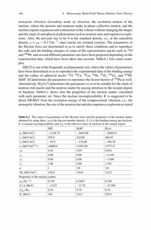
146 6 Microscopic Mean-Field Theory (Hartree–Fock Theory)
monopole vibration (breathing mode of vibration; the excitation motion of thenucleus, where the protons and neutrons make in phase collective motion, and thenucleus repeats expansion and contraction of the volumewithout changing the shape)and the study of astrophysical phenomena such as neutron stars and supernova explo-sions. Also, the pressure has to be 0 at the standard density, i.e., at the saturationdensity ρ = ρ0 ∼ 0.17 fm−3, since nuclei are isolated systems. The parameters ofthe Skyrme force are determined so as to satisfy these conditions and to reproducethe radii and the binding energies of some of the representative nuclei such as 16Oand 208Pb, and several different parameter sets have been proposed depending on theexperimental data, which have been taken into account. Table6.1 lists some exam-ples.
SIII [5] is one of the frequently used parameter sets,where the values of parametershave been determined so as to reproduce the experimental data of the binding energyand the radius of spherical nuclei 16O, 40Ca, 48Ca, 56Ni, 90Zr, 140Ce, and 208Pb.SkM∗ [6] determines the parameters to reproduce the fission barrier of 240Pu as well.Alternatively, SLy4 [7] determines the parameters so as to be suitable for the study ofneutron-rich nuclei and the neutron matter by paying attention to the isospin degreeof freedom. Table6.1 shows also the properties of the nuclear matter calculatedwith each parameter set. Since the nuclear incompressibility K is suggested to beabout 200MeV from the excitation energy of the compressional vibration, i.e., themonopole vibration, the size of the neutron star and also supernova explosion as stated
Table 6.1 The values of parameters of the Skyrme force and the properties of the nuclear matterobtained by using them. ρ0 is the baryon number density, E/A is the binding energy per nucleon,K is nuclear incompressibility and m∗
N is the effective mass of nucleon in the central region
SIII SkM∗ SLy4
t0 (MeVfm3) −1128.75 −2645.00 −2488.91
t1 (MeVfm5) 395.0 410.00 486.82
t2 (MeVfm5) −95.0 −135.00 −546.39
t3 (MeVfm3+α) 14000.0 15595.00 13777.0
x0 0.45 0.09 0.834
x1 0.00 0.00 −0.344
x2 0.00 0.00 −1.000
x3 1.00 0.00 1.354
α 1 1/6 1/6
W0 (MeVfm5) 120.0 130.0 123.0
Properties of the nuclear matter
ρ0 (fm−3) 0.145 0.1603 0.160
E/A (MeV) −15.87 −15.78 −15.969
m∗N /MN 0.76 0.79 0.70
K (MeV) 356 216.7 229.9
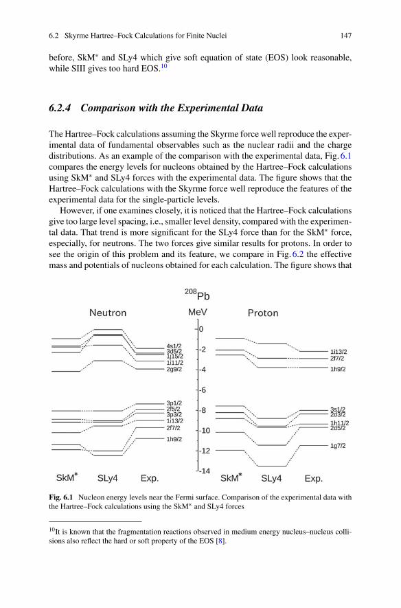
6.2 Skyrme Hartree–Fock Calculations for Finite Nuclei 147
before, SkM∗ and SLy4 which give soft equation of state (EOS) look reasonable,while SIII gives too hard EOS.10
6.2.4 Comparison with the Experimental Data
The Hartree–Fock calculations assuming the Skyrme force well reproduce the exper-imental data of fundamental observables such as the nuclear radii and the chargedistributions. As an example of the comparison with the experimental data, Fig. 6.1compares the energy levels for nucleons obtained by the Hartree–Fock calculationsusing SkM∗ and SLy4 forces with the experimental data. The figure shows that theHartree–Fock calculations with the Skyrme force well reproduce the features of theexperimental data for the single-particle levels.
However, if one examines closely, it is noticed that the Hartree–Fock calculationsgive too large level spacing, i.e., smaller level density, compared with the experimen-tal data. That trend is more significant for the SLy4 force than for the SkM∗ force,especially, for neutrons. The two forces give similar results for protons. In order tosee the origin of this problem and its feature, we compare in Fig. 6.2 the effectivemass and potentials of nucleons obtained for each calculation. The figure shows that
Fig. 6.1 Nucleon energy levels near the Fermi surface. Comparison of the experimental data withthe Hartree–Fock calculations using the SkM∗ and SLy4 forces
10It is known that the fragmentation reactions observed in medium energy nucleus–nucleus colli-sions also reflect the hard or soft property of the EOS [8].
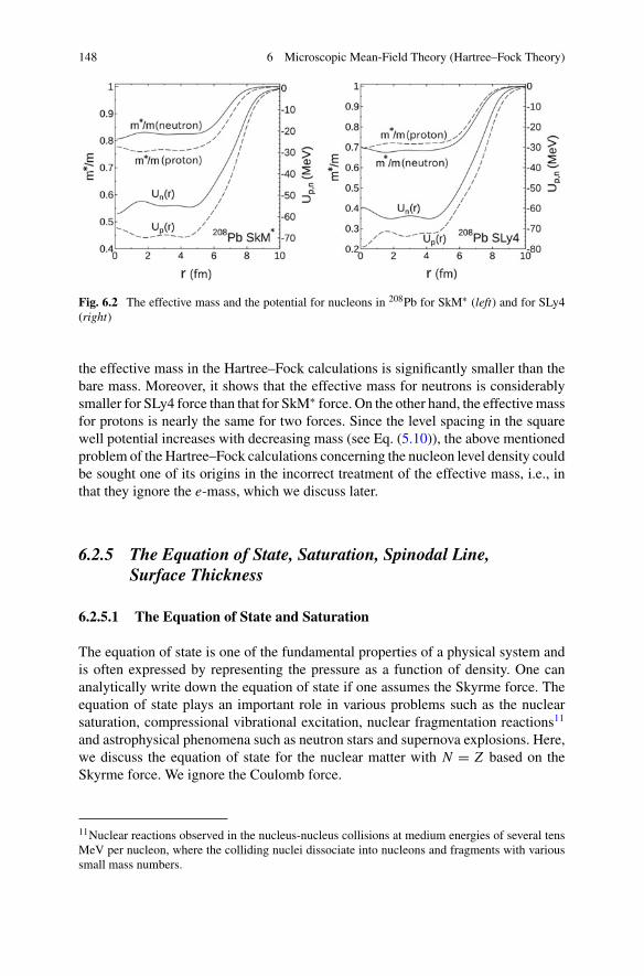
148 6 Microscopic Mean-Field Theory (Hartree–Fock Theory)
Fig. 6.2 The effective mass and the potential for nucleons in 208Pb for SkM∗ (left) and for SLy4(right)
the effective mass in the Hartree–Fock calculations is significantly smaller than thebare mass. Moreover, it shows that the effective mass for neutrons is considerablysmaller for SLy4 force than that for SkM∗ force. On the other hand, the effectivemassfor protons is nearly the same for two forces. Since the level spacing in the squarewell potential increases with decreasing mass (see Eq. (5.10)), the above mentionedproblem of the Hartree–Fock calculations concerning the nucleon level density couldbe sought one of its origins in the incorrect treatment of the effective mass, i.e., inthat they ignore the e-mass, which we discuss later.
6.2.5 The Equation of State, Saturation, Spinodal Line,Surface Thickness
6.2.5.1 The Equation of State and Saturation
The equation of state is one of the fundamental properties of a physical system andis often expressed by representing the pressure as a function of density. One cananalytically write down the equation of state if one assumes the Skyrme force. Theequation of state plays an important role in various problems such as the nuclearsaturation, compressional vibrational excitation, nuclear fragmentation reactions11
and astrophysical phenomena such as neutron stars and supernova explosions. Here,we discuss the equation of state for the nuclear matter with N = Z based on theSkyrme force. We ignore the Coulomb force.
11Nuclear reactions observed in the nucleus-nucleus collisions at medium energies of several tensMeV per nucleon, where the colliding nuclei dissociate into nucleons and fragments with varioussmall mass numbers.
6.2 Skyrme Hartree–Fock Calculations for Finite Nuclei 149
The pressure at finite temperature is given by the derivative of the Helmholtz freeenergy F = E − T S:
P = −(
∂
∂VF
)T
. (6.49)
Since the internal energy E is given by the sum of the interaction energy Eint andthe kinetic energy Ekin, we divide the pressure into the part originating from theinteraction energy and that from the kinetic energy
P = PV + PT . (6.50)
(1)Pressuredue to the InteractionEnergy: PV Weestimate the pressure originatingfrom the interaction by replacing the total energy E with the interaction energy Eint
in the formula (6.48) at zero temperature. Corresponding to Eq. (6.46), let us assumethat the interaction energy per nucleon is given by
Eint
A= −C1ρ + C2ρ
1+α . (6.51)
We have changed the power in the second term on the right-hand side of Eq. (6.51) byconsidering the general case when the nuclear force is given by Eq. (6.29) instead ofEq. (6.28), although Eq. (6.46) corresponds to the case when α = 1.12 The pressuredue to the interaction is then given by
PV = −C1ρ2 + (1 + α)C2ρ
2+α . (6.52)
(2) Pressure due to the Kinetic Energy: PT In order to obtain the pressure due tothe kinetic energy, we first calculate the kinetic energy per unit volume based on
Ekin
V= 4
(2π)3
∫d3k
�2k2
2MN
1
exp[( �2k22MN
− λ)/T ] + 1, (6.53)
then obtain PT by inserting Ekin in the place of E in Bernoulli’s formula [9, 10],
PV = 2
3E , (6.54)
which holds for both classical and quantum mechanical ideal gases irrespective ofthe statistical property. λ in Eq. (6.53) is the Fermi level or Fermi potential.(2a) The Degenerate Limit: the Case of T = 0 When T = 0, one can easily showthat
12The prescriptionwhich takes into account the finite range property of the nuclear force through thet1 and t2 terms following Skyrme would need to be reconsidered when we use α smaller than 2/3 indiscussing the saturation, since the last term on the right-hand side of Eq. (6.46) is proportional toρ5/3.
150 6 Microscopic Mean-Field Theory (Hartree–Fock Theory)
PT = 2
5ρεF = 2
5ρ
�2k2
F
2MN∝ ρ5/3 , (6.55)
where εF is the Fermi level or Fermi energy at T = 0.(2b) The Case of Non-degenerate System at High Temperature:At high temperatures,one can approximate the Fermi distribution by the Boltzmann distribution. We thenhave
Ekin
V∼ 4
(2π)34π
�2
2MN
∫ ∞
0dkk4e−( �
2k2
2MN−λ)/T
∼ 4
(2π)34π
1
2MN
1
�3eλ/T 3
8
√π(2MN T )5/2 , (6.56)
N
V∼ 4
(2π)34π∫ ∞
0dkk2e−( �
2k2
2MN−λ)/T
∼ 4
(2π)34π
1
�3eλ/T 1
4
√π(2MN T )3/2 , (6.57)
and obtainEkin
V= 3
2ρT . (6.58)
Using Bernoulli’s formula, the pressure due to the kinetic energy is finally given by
PT = ρT , (6.59)
which is well known for the ideal gas.(2c) The Case of Fermi Gas at Low Temperature: The kinetic energy at temperatureT is given by
Ekin(T ) = Ekin(T = 0) + 1
4
π2
εFAT 2 (6.60)
when the temperature T satisfies the condition T λ. The pressure due to the kineticenergy is therefore given by
P = 2
5ρεF
[1 + 5
12π2
(T
εF
)2]
(6.61)
by using Eq. (6.54).Let us guess the behaviour of the equation of state based on these results. We first
consider the case when the temperature is 0. Equations (6.52) and (6.55) suggest thatthe effect of kinetic energy, i.e., the degeneracy pressure, dominates in the regionof low density and the pressure is positive and increases with density. Eventually,the pressure due to attractive two-body interaction becomes to overcome and the
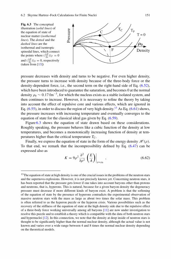
6.2 Skyrme Hartree–Fock Calculations for Finite Nuclei 151
Fig. 6.3 The conceptualillustration (solid lines) ofthe equation of state ofnuclear matter (isothermallines). The dotted and thedashed lines are theisothermal and isentropicspinodal lines, which connectthe points where ( ∂ P
∂ρ)|T = 0
and ( ∂ P∂ρ
)|S = 0, respectively(taken from [13])
pressure decreases with density and turns to be negative. For even higher density,the pressure turns to increase with density because of the three-body force or thedensity-dependent force, i.e., the second term on the right-hand side of Eq. (6.52),which have been introduced to guarantee the saturation, and becomes 0 at the normaldensity ρ0 ∼ 0.17 fm−3, for which the nucleus exists as a stable isolated system, andthen continues to increase. However, it is necessary to refine the theory by takinginto account the effect of repulsive core and various effects, which are ignored inEq. (6.55), in order to discuss the region of very high density.13 As Eq. (6.61) shows,the pressure increases with increasing temperature and eventually converges to theequation of state for the classical ideal gas given by Eq. (6.59).
Figure6.3 shows the equation of state drawn based on these considerations.Roughly speaking, the pressure behaves like a cubic function of the density at lowtemperatures, and becomes a monotonically increasing function of density at tem-peratures higher than the critical temperature TC.
Finally, we express the equation of state in the form of the energy densityH (ρ).To that end, we remark that the incompressibility defined by Eq. (6.47) can beexpressed also as
K = 9ρ2 ∂2
∂ρ2
(E
A
)∣∣∣∣ρ=ρ0
, (6.62)
13The equation of state at high density is one of the crucial issues in the problems of the neutron starsand the supernova explosions. However, it is not precisely known yet. Concerning neutron stars, ithas been reported that the pressure gets lower if one takes into account baryons other than protonsand neutrons, that is, hyperons. This is natural, because for a given baryon density the degeneracypressure must decrease if more different kinds of baryon exist. A problem is that the softeningof the equation of state by the presence of hyperons contradicts the experimental observation ofmassive neutron stars with the mass as large as about two times the solar mass. This problemis often referred to as the hyperon puzzle or the hyperon crisis. Various possibilities such as therecovery of the stiffness of the equation of state at the high density side due to the repulsive effectof a three-body force working universally among all baryons [11] are now under investigation toresolve this puzzle and to establish a theory which is compatible with the data of both neutron starsand hypernuclei [12]. In this connection, we note that the density at deep inside of neutron stars isthought to be significantly higher than the normal nuclear density, although the actual value is notknown and varies over a wide range between 4 and 8 times the normal nuclear density dependingon the theoretical models.
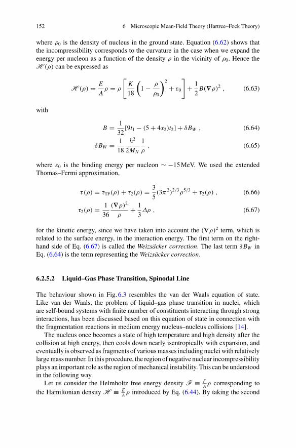
152 6 Microscopic Mean-Field Theory (Hartree–Fock Theory)
where ρ0 is the density of nucleus in the ground state. Equation (6.62) shows thatthe incompressibility corresponds to the curvature in the case when we expand theenergy per nucleon as a function of the density ρ in the vicinity of ρ0. Hence theH (ρ) can be expressed as
H (ρ) = E
Aρ = ρ
[K
18
(1 − ρ
ρ0
)2
+ ε0
]+ 1
2B(∇ρ)2 , (6.63)
with
B = 1
32[9t1 − (5 + 4x2)t2] + δBW , (6.64)
δBW = 1
18
�2
2MN
1
ρ, (6.65)
where ε0 is the binding energy per nucleon ∼ −15MeV. We used the extendedThomas–Fermi approximation,
τ(ρ) = τTF(ρ) + τ2(ρ) = 3
5(3π2)2/3ρ5/3 + τ2(ρ) , (6.66)
τ2(ρ) = 1
36
(∇ρ)2
ρ+ 1
3Δρ , (6.67)
for the kinetic energy, since we have taken into account the (∇ρ)2 term, which isrelated to the surface energy, in the interaction energy. The first term on the right-hand side of Eq. (6.67) is called the Weizsäcker correction. The last term δBW inEq. (6.64) is the term representing the Weizsäcker correction.
6.2.5.2 Liquid–Gas Phase Transition, Spinodal Line
The behaviour shown in Fig. 6.3 resembles the van der Waals equation of state.Like van der Waals, the problem of liquid–gas phase transition in nuclei, whichare self-bound systems with finite number of constituents interacting through stronginteractions, has been discussed based on this equation of state in connection withthe fragmentation reactions in medium energy nucleus–nucleus collisions [14].
The nucleus once becomes a state of high temperature and high density after thecollision at high energy, then cools down nearly isentropically with expansion, andeventually is observed as fragments of variousmasses including nucleiwith relativelylargemass number. In this procedure, the region of negative nuclear incompressibilityplays an important role as the region ofmechanical instability. This can be understoodin the following way.
Let us consider the Helmholtz free energy density F ≡ FA ρ corresponding to
the Hamiltonian density H ≡ EA ρ introduced by Eq. (6.44). By taking the second
6.2 Skyrme Hartree–Fock Calculations for Finite Nuclei 153
Fig. 6.4 The unstable region(the oblique lines: theboundary is called thespinodal line) and thecompressed region (shadedregion) which is expected tolead to the fragmentationreaction in heavy-ioncollisions. The dotted line isan example of the trajectoryin heavy-ion collisions. Thefigure is after D.K. Scott
derivative ofF with respect to the density, we have
∂2F
∂ρ2= 2
∂
∂ρ
(F
A
)+ ρ
∂2
∂ρ2
(F
A
). (6.68)
On the other hand, from the definition of pressure (6.49), we have
∂ P
∂ρ= 2ρ
∂
∂ρ
(F
A
)+ ρ2 ∂2
∂ρ2
(F
A
). (6.69)
Equations (6.68) and (6.69) lead to the relationship,
∂2F
∂ρ2= 1
ρ
∂ P
∂ρ. (6.70)
This relationship shows that the negative gradient of the pressure, i.e., negative incom-pressibility, is equivalent to that the second derivative of the free energy density withrespect to density is negative.
∂ P
∂ρ< 0 ↔ ∂2F
∂ρ2< 0 . (6.71)
The condition ∂2F∂ρ2 < 0 means that the system is unstable with respect to the density
fluctuation, i.e., themechanical instability. It is because the change of the free energydensity due to a local fluctuation of the density is given by
ΔF = 1
2[F (ρ + Δρ) + F (ρ − Δρ)] − F (ρ)
= 1
2
∂2F
∂ρ2(Δρ)2 , (6.72)
154 6 Microscopic Mean-Field Theory (Hartree–Fock Theory)
and it becomes ΔF < 0 if ∂2F∂ρ2 < 0. The former, i.e., ΔF < 0, means that the free
energy gets lower in the state with density fluctuation.Figure6.4 shows the mechanically unstable region, whose boundary is called the
spinodal line, and the region which is compressed immediately after the collisionand is expected to be required in order to reach instability region after cooling in thenucleus–nucleus collision at medium energies.
6.2.5.3 Surface Diffuseness
The surface property of nuclei is one of the intriguing physical quantities concern-ing nuclear structure as well as nuclear reactions. Equation (6.63) suggests that theparameter B given by Eq. (6.64) is related to the surface thickness. In fact, usingEq. (6.63) one can show [15] that the density distribution of nuclei is given by
ρ = ρ0 tanh2
(r − R
2b
), (6.73)
b2 = 9B
Kρ0 . (6.74)
If we approximate the functional form of Eq. (6.73) by the standard Woods–Saxontype, then the surface diffuseness parameter a is given by a ≈ 2b/3. Equations (6.74)and (6.64) suggest that the surface thickness of nuclei is governed by the nuclearincompressibility and the Weizsäcker term in the asymptotic surface region, wherethe density is extremely small, or by the range of nuclear force through the parameter9t1 − (5 + 4x2)t2 in more inside region.
6.2.6 Beyond the Hartree–Fock Calculations:Nucleon–Vibration Coupling; ω-Mass
We remarked in Sect. 6.2.4 that the single-particle level density obtained by theHartree–Fock calculations is too small compared with the experimental data, andsuggested the possibility that one of the reasons of this failure is related to theeffective mass.
The effective mass hitherto discussed within the framework of the Hartree–Focktheory arises from the antisymmetrization of nucleons. In revised theories which gobeyond the Hartree–Fock approximation, the single-particle potential has an energydependent correction term in addition to the potentialUHF in theHartree–Fock theorydue to, e.g., the coupling of nucleons to the surface vibration, which is one of thenuclear collective excitations. In consequence, the energy of the single-particle stateis given by
e = p2
2m+ UHF(r, p(r)) + UPVC(r, e) . (6.75)
6.2 Skyrme Hartree–Fock Calculations for Finite Nuclei 155
The lower index PVC in the third term on the right-hand side means particle–vibration coupling. We denoted the bare nucleon mass MN by m. Also, we rep-resented the Hartree–Fock potential by an equivalent momentum dependent localpotential in the spirit of the WKB approximation, although it is in general a non-local potential.
By taking the derivative of both sides of Eq. (6.75) with respect to p, and usingthe definition of the effective mass 1
m∗ ≡ 1pdedp , we obtain
m∗
m= mk
m
mω
m, (6.76)
mk
m=(1 + m
p
∂UHF
∂p
)−1
, (6.77)
mω
m= 1 − ∂UPVC
∂e, (6.78)
where mk stands for k-mass and mω for ω-mass or e-mass.The ω-mass mω is larger than the bare mass m, and is concentrated in the surface
region reflecting the coupling between nucleons and the surface vibrational motion[16]. Thanks to the ω-mass, the final effective mass becomes larger than the k-mass introduced in the Hartree–Fock approximation. Hence the agreement betweenthe theoretical value and the experimental data concerning the single-particle leveldensity is improved by taking into account the effect of particle–vibration coupling.
Incidentally, this is related to the fact that the parameter a,14 which is called thelevel density parameter, takes the value A/8MeV−1 in the region of low excitationenergy in contradiction to the expectation. The ω-mass approaches 1 with increas-ing excitation energy. Consequently, the level density parameter a is expected toapproach the expected value A/15MeV−1 as the excitation energy increases. It hasbeen confirmed that it is the case indeed from the study of, e.g., the excitation energydependence of the evaporation spectrum of α particles from excited nuclei [18].
6.3 Relativistic Mean-Field Theory (σωρ Model)
Theoretical studies which use the relativistic theory and introduce mesons to mediatethe nuclear force have also been extensively developed to determine nuclear proper-ties such as the binding energy and the shape of nuclei within the framework of themean-field theory in parallel with the non-relativistic Hartree–Fock theory with theSkyrme force. The relativistic approach has the advantage that the spin–orbit force is
14If one considers the nucleus as a Fermi gas, then the level density ρL exponentially increases withthe excitation energy E and can be roughly given by ρL (E) ∼ exp(aE)1/2 (see [17] for details).
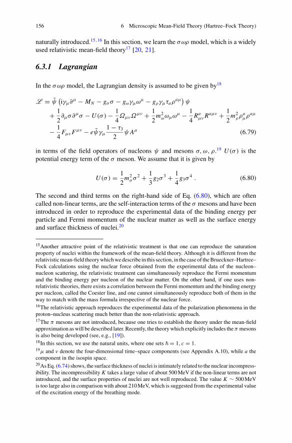
156 6 Microscopic Mean-Field Theory (Hartree–Fock Theory)
naturally introduced.15,16 In this section, we learn the σωρ model, which is a widelyused relativistic mean-field theory17 [20, 21].
6.3.1 Lagrangian
In the σωρ model, the Lagrangian density is assumed to be given by18
L = ψ(iγμ∂μ − MN − gσ σ − gωγμωμ − gργμτaρ
aμ)ψ
+ 1
2∂μσ∂μσ − U (σ ) − 1
4ΩμνΩ
μν + 1
2m2
ωωμωμ − 1
4Ra
μν Raμν + 1
2m2
ρρaμρaμ
− 1
4Fμν Fμν − eψγμ
1 − τ3
2ψ Aμ (6.79)
in terms of the field operators of nucleons ψ and mesons σ, ω, ρ.19 U (σ ) is thepotential energy term of the σ meson. We assume that it is given by
U (σ ) = 1
2m2
σ σ 2 + 1
3g2σ
3 + 1
4g3σ
4 . (6.80)
The second and third terms on the right-hand side of Eq. (6.80), which are oftencalled non-linear terms, are the self-interaction terms of the σ mesons and have beenintroduced in order to reproduce the experimental data of the binding energy perparticle and Fermi momentum of the nuclear matter as well as the surface energyand surface thickness of nuclei.20
15Another attractive point of the relativistic treatment is that one can reproduce the saturationproperty of nuclei within the framework of the mean-field theory. Although it is different from therelativisticmean-field theorywhichwedescribe in this section, in the case of theBrueckner–Hartree–Fock calculations using the nuclear force obtained from the experimental data of the nucleon–nucleon scattering, the relativistic treatment can simultaneously reproduce the Fermi momentumand the binding energy per nucleon of the nuclear matter. On the other hand, if one uses non-relativistic theories, there exists a correlation between the Fermi momentum and the binding energyper nucleon, called the Coester line, and one cannot simultaneously reproduce both of them in theway to match with the mass formula irrespective of the nuclear force.16The relativistic approach reproduces the experimental data of the polarization phenomena in theproton–nucleus scattering much better than the non-relativistic approach.17The π mesons are not introduced, because one tries to establish the theory under the mean-fieldapproximation aswill be described later. Recently, the theorywhich explicitly includes theπ mesonsis also being developed (see, e.g., [19]).18In this section, we use the natural units, where one sets � = 1, c = 1.19μ and ν denote the four-dimensional time–space components (see Appendix A.10), while a thecomponent in the isospin space.20AsEq. (6.74) shows, the surface thickness of nuclei is intimately related to the nuclear incompress-ibility. The incompressibility K takes a large value of about 500MeV if the non-linear terms are notintroduced, and the surface properties of nuclei are not well reproduced. The value K ∼ 500MeVis too large also in comparison with about 210MeV, which is suggested from the experimental valueof the excitation energy of the breathing mode.
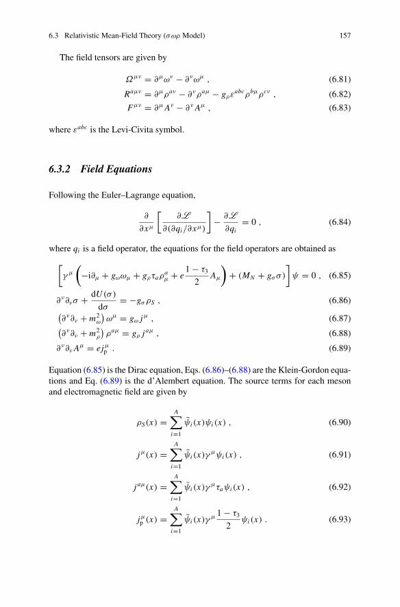
6.3 Relativistic Mean-Field Theory (σωρ Model) 157
The field tensors are given by
Ωμν = ∂μων − ∂νωμ , (6.81)
Raμν = ∂μρaν − ∂νρaμ − gρεabcρbμρcν , (6.82)
Fμν = ∂μ Aν − ∂ν Aμ , (6.83)
where εabc is the Levi-Civita symbol.
6.3.2 Field Equations
Following the Euler–Lagrange equation,
∂
∂xμ
[∂L
∂(∂qi/∂xμ)
]− ∂L
∂qi= 0 , (6.84)
where qi is a field operator, the equations for the field operators are obtained as
[γ μ
(−i∂μ + gωωμ + gρτaρ
aμ + e
1 − τ3
2Aμ
)+ (MN + gσ σ )
]ψ = 0 , (6.85)
∂ν∂νσ + dU (σ )
dσ= −gσ ρS , (6.86)(
∂ν∂ν + m2ω
)ωμ = gω jμ , (6.87)(
∂ν∂ν + m2ρ
)ρaμ = gρ j aμ , (6.88)
∂ν∂ν Aμ = ejμp . (6.89)
Equation (6.85) is the Dirac equation, Eqs. (6.86)–(6.88) are the Klein-Gordon equa-tions and Eq. (6.89) is the d’Alembert equation. The source terms for each mesonand electromagnetic field are given by
ρS(x) =A∑
i=1
ψi (x)ψi (x) , (6.90)
jμ(x) =A∑
i=1
ψi (x)γ μψi (x) , (6.91)
j aμ(x) =A∑
i=1
ψi (x)γ μτaψi (x) , (6.92)
jμp (x) =
A∑i=1
ψi (x)γ μ 1 − τ3
2ψi (x) . (6.93)
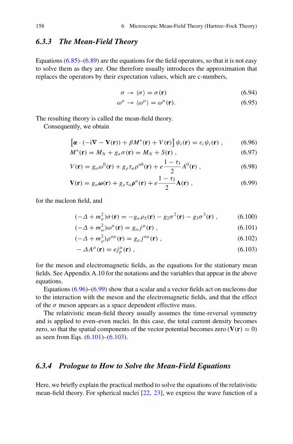
158 6 Microscopic Mean-Field Theory (Hartree–Fock Theory)
6.3.3 The Mean-Field Theory
Equations (6.85)–(6.89) are the equations for the field operators, so that it is not easyto solve them as they are. One therefore usually introduces the approximation thatreplaces the operators by their expectation values, which are c-numbers,
σ → 〈σ 〉 = σ(r) (6.94)
ωμ → 〈ωμ〉 = ωμ(r). (6.95)
The resulting theory is called the mean-field theory.Consequently, we obtain
[α · (−i∇ − V(r)) + βM∗(r) + V (r)
]ψi (r) = εiψi (r) , (6.96)
M∗(r) = MN + gσ σ (r) = MN + S(r) , (6.97)
V (r) = gωω0(r) + gρτaρa0(r) + e
1 − τ3
2A0(r) , (6.98)
V(r) = gωω(r) + gρτaρa(r) + e
1 − τ3
2A(r) , (6.99)
for the nucleon field, and
(−Δ + m2σ )σ (r) = −gσ ρS(r) − g2σ
2(r) − g3σ3(r) , (6.100)
(−Δ + m2ω)ωμ(r) = gω jμ(r) , (6.101)
(−Δ + m2ρ)ρ
aμ(r) = gρ j aμ(r) , (6.102)
− ΔAμ(r) = ejμp (r) , (6.103)
for the meson and electromagnetic fields, as the equations for the stationary meanfields. See Appendix A.10 for the notations and the variables that appear in the aboveequations.
Equations (6.96)–(6.99) show that a scalar and a vector fields act on nucleons dueto the interaction with the meson and the electromagnetic fields, and that the effectof the σ meson appears as a space dependent effective mass.
The relativistic mean-field theory usually assumes the time-reversal symmetryand is applied to even–even nuclei. In this case, the total current density becomeszero, so that the spatial components of the vector potential becomes zero (V(r) = 0)as seen from Eqs. (6.101)–(6.103).
6.3.4 Prologue to How to Solve the Mean-Field Equations
Here, we briefly explain the practical method to solve the equations of the relativisticmean-field theory. For spherical nuclei [22, 23], we express the wave function of a
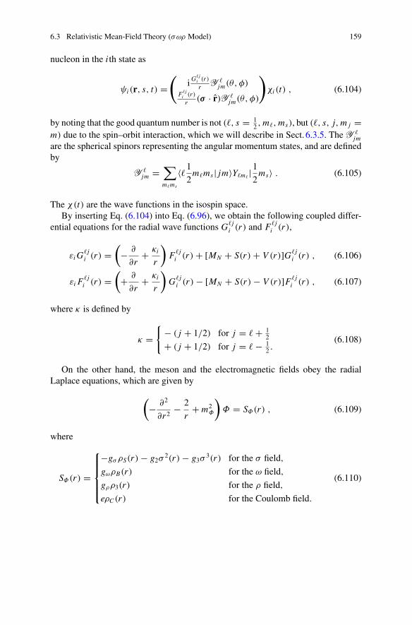
6.3 Relativistic Mean-Field Theory (σωρ Model) 159
nucleon in the i th state as
ψi (r, s, t) =(
iG�ji (r)
r Y �jm(θ, φ)
F�ji (r)
r (σ · r)Y �jm(θ, φ)
)χi (t) , (6.104)
by noting that the good quantum number is not (�, s = 12 , m�, ms), but (�, s, j, m j =
m) due to the spin–orbit interaction, which we will describe in Sect. 6.3.5. The Y �jm
are the spherical spinors representing the angular momentum states, and are definedby
Y �jm =
∑m�ms
〈�12
m�ms | jm〉Y�m�|12
ms〉 . (6.105)
The χ(t) are the wave functions in the isospin space.By inserting Eq. (6.104) into Eq. (6.96), we obtain the following coupled differ-
ential equations for the radial wave functions G�ji (r) and F�j
i (r),
εi G�ji (r) =
(− ∂
∂r+ κi
r
)F�j
i (r) + [MN + S(r) + V (r)]G�ji (r) , (6.106)
εi F�ji (r) =
(+ ∂
∂r+ κi
r
)G�j
i (r) − [MN + S(r) − V (r)]F�ji (r) , (6.107)
where κ is defined by
κ ={
− ( j + 1/2) for j = � + 12
+ ( j + 1/2) for j = � − 12 .
(6.108)
On the other hand, the meson and the electromagnetic fields obey the radialLaplace equations, which are given by
(− ∂2
∂r2− 2
r+ m2
Φ
)Φ = SΦ(r) , (6.109)
where
SΦ(r) =
⎧⎪⎪⎪⎨⎪⎪⎪⎩
−gσ ρS(r) − g2σ 2(r) − g3σ 3(r) for the σ field,
gωρB(r) for the ω field,
gρρ3(r) for the ρ field,
eρC(r) for the Coulomb field.
(6.110)
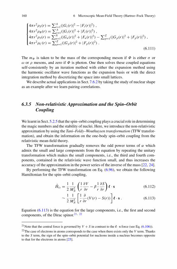
160 6 Microscopic Mean-Field Theory (Hartree–Fock Theory)
⎧⎪⎪⎪⎨⎪⎪⎪⎩
4πr2ρS(r) =∑Ai=1(|Gi (r)|2 − |Fi (r)|2) ,
4πr2ρB(r) =∑Ai=1(|Gi (r)|2 + |Fi (r)|2) ,
4πr2ρ3(r) =∑Nn=1(|Gn(r)|2 + |Fn(r)|2) −∑Z
p=1(|G p(r)|2 + |Fp(r)|2) ,
4πr2ρC(r) =∑Zp=1(|G p(r)|2 + |Fp(r)|2) .
(6.111)
The mΦ is taken to be the mass of the corresponding meson if Φ is either σ orω or ρ mesons, and zero if Φ is photon. One then solves these coupled equationsself-consistently by an iteration method with either the expansion method usingthe harmonic oscillator wave functions as the expansion basis or with the directintegration method by discretizing the space into small lattices.
We describe actual applications in Sect. 7.6.2 by taking the study of nuclear shapeas an example after we learn pairing correlations.
6.3.5 Non-relativistic Approximation and the Spin–OrbitCoupling
We learnt in Sect. 5.2.5 that the spin–orbit coupling plays a crucial role in determiningthe magic numbers and the stability of nuclei. Here, we introduce the non-relativisticapproximation by using the Tani–Foldy–Wouthuysen transformation (TFW transfor-mation), and obtain the information on the one-body spin–orbit coupling from therelativistic mean-field theory.
The TFW transformation gradually removes the odd power terms of α whichadmix the small and large components from the equation by repeating the unitarytransformation which makes the small components, i.e., the third and fourth com-ponents, contained in the relativistic wave function small, and thus increases theaccuracy of the approximation in the power series of the inverse of the mass [22, 24].
By performing the TFW transformation on Eq. (6.96), we obtain the followingHamiltonian for the spin–orbit coupling,
H�s = 1
2
1
M2N
(1
r
∂V
∂r− β
1
r
∂S
∂r
)� · s (6.112)
∼ 1
2
1
M2N
[1
r
∂
∂r(V (r) − S(r))
]� · s . (6.113)
Equation (6.113) is the equation for the large components, i.e., the first and secondcomponents, of the Dirac spinor.21, 22
21Note that the central force is governed by V + S in contrast to the � · s force (see Eq. (6.106)).22The case of electrons in atoms corresponds to the case when there exists only the V term. Thanksto the S term, the sign of the spin–orbit potential for nucleons inside a nucleus becomes oppositeto that for the electrons in atoms [25].
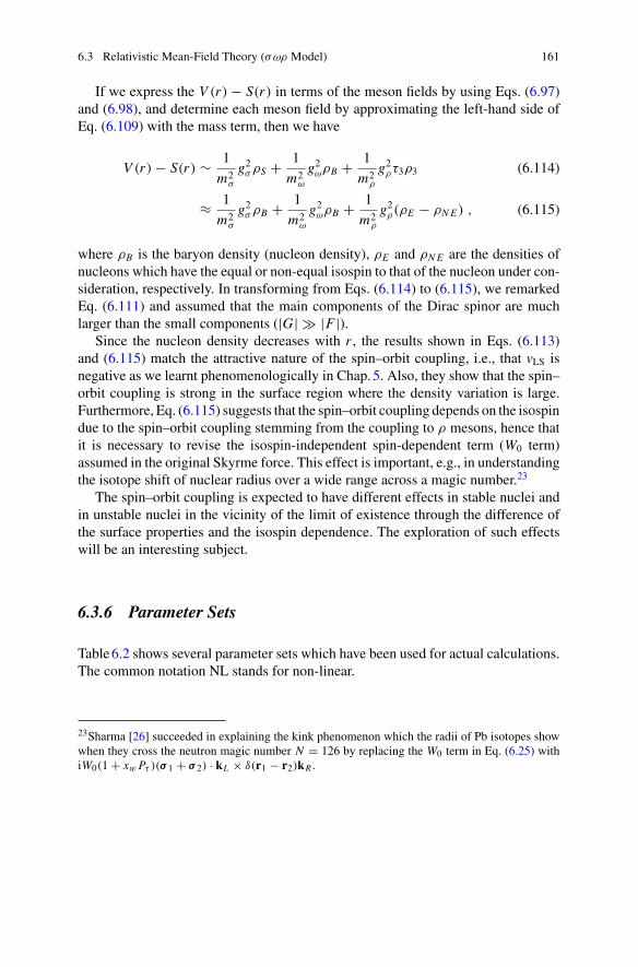
6.3 Relativistic Mean-Field Theory (σωρ Model) 161
If we express the V (r) − S(r) in terms of the meson fields by using Eqs. (6.97)and (6.98), and determine each meson field by approximating the left-hand side ofEq. (6.109) with the mass term, then we have
V (r) − S(r) ∼ 1
m2σ
g2σ ρS + 1
m2ω
g2ωρB + 1
m2ρ
g2ρτ3ρ3 (6.114)
≈ 1
m2σ
g2σ ρB + 1
m2ω
g2ωρB + 1
m2ρ
g2ρ(ρE − ρN E ) , (6.115)
where ρB is the baryon density (nucleon density), ρE and ρN E are the densities ofnucleons which have the equal or non-equal isospin to that of the nucleon under con-sideration, respectively. In transforming from Eqs. (6.114) to (6.115), we remarkedEq. (6.111) and assumed that the main components of the Dirac spinor are muchlarger than the small components (|G| � |F |).
Since the nucleon density decreases with r , the results shown in Eqs. (6.113)and (6.115) match the attractive nature of the spin–orbit coupling, i.e., that vLS isnegative as we learnt phenomenologically in Chap.5. Also, they show that the spin–orbit coupling is strong in the surface region where the density variation is large.Furthermore, Eq. (6.115) suggests that the spin–orbit coupling depends on the isospindue to the spin–orbit coupling stemming from the coupling to ρ mesons, hence thatit is necessary to revise the isospin-independent spin-dependent term (W0 term)assumed in the original Skyrme force. This effect is important, e.g., in understandingthe isotope shift of nuclear radius over a wide range across a magic number.23
The spin–orbit coupling is expected to have different effects in stable nuclei andin unstable nuclei in the vicinity of the limit of existence through the difference ofthe surface properties and the isospin dependence. The exploration of such effectswill be an interesting subject.
6.3.6 Parameter Sets
Table6.2 shows several parameter sets which have been used for actual calculations.The common notation NL stands for non-linear.
23Sharma [26] succeeded in explaining the kink phenomenon which the radii of Pb isotopes showwhen they cross the neutron magic number N = 126 by replacing the W0 term in Eq. (6.25) withiW0(1 + xw Pτ )(σ 1 + σ 2) · kL × δ(r1 − r2)kR .
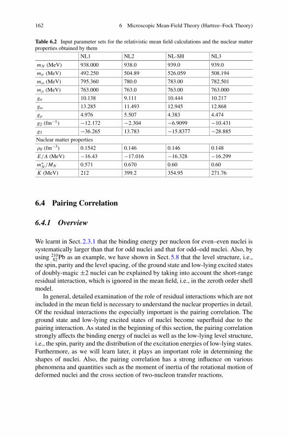
162 6 Microscopic Mean-Field Theory (Hartree–Fock Theory)
Table 6.2 Input parameter sets for the relativistic mean field calculations and the nuclear matterproperties obtained by them
NL1 NL2 NL-SH NL3
m N (MeV) 938.000 938.0 939.0 939.0
mσ (MeV) 492.250 504.89 526.059 508.194
mω (MeV) 795.360 780.0 783.00 782.501
mρ (MeV) 763.000 763.0 763.00 763.000
gσ 10.138 9.111 10.444 10.217
gω 13.285 11.493 12.945 12.868
gρ 4.976 5.507 4.383 4.474
g2 (fm−1) −12.172 −2.304 −6.9099 −10.431
g3 −36.265 13.783 −15.8377 −28.885
Nuclear matter properties
ρ0 (fm−3) 0.1542 0.146 0.146 0.148
E/A (MeV) −16.43 −17.016 −16.328 −16.299
m∗N /MN 0.571 0.670 0.60 0.60
K (MeV) 212 399.2 354.95 271.76
6.4 Pairing Correlation
6.4.1 Overview
We learnt in Sect. 2.3.1 that the binding energy per nucleon for even–even nuclei issystematically larger than that for odd nuclei and that for odd–odd nuclei. Also, byusing 210
82 Pb as an example, we have shown in Sect. 5.8 that the level structure, i.e.,the spin, parity and the level spacing, of the ground state and low-lying excited statesof doubly-magic ±2 nuclei can be explained by taking into account the short-rangeresidual interaction, which is ignored in the mean field, i.e., in the zeroth order shellmodel.
In general, detailed examination of the role of residual interactions which are notincluded in the mean field is necessary to understand the nuclear properties in detail.Of the residual interactions the especially important is the pairing correlation. Theground state and low-lying excited states of nuclei become superfluid due to thepairing interaction. As stated in the beginning of this section, the pairing correlationstrongly affects the binding energy of nuclei as well as the low-lying level structure,i.e., the spin, parity and the distribution of the excitation energies of low-lying states.Furthermore, as we will learn later, it plays an important role in determining theshapes of nuclei. Also, the pairing correlation has a strong influence on variousphenomena and quantities such as the moment of inertia of the rotational motion ofdeformed nuclei and the cross section of two-nucleon transfer reactions.
6.4 Pairing Correlation 163
The pairing interaction among electrons, which makes metals superfluid, isinduced through the electron–phonon coupling [27]. In contrast, the pairing correla-tion in nuclei originates partly from the direct attractive interaction between nucleonsand partly from the mechanism that the pair of nucleons, which occupy time-reversalstates to each other in the vicinity of Fermi surface, form a Cooper pair via surfacevibrations (see Ref. [28] for details).
In solid state physics, the origin of superfluidity depends on the system. Forexample, it is known that many metals and alloys become superfluid by the 1S pair,while heavy electron systems and liquid 3He become superfluid by 3P pair [27]. Themechanism to become superfluid depends on the system for the nucleus as well. Inthis section, by having the ground and low-lying excited states of stable nuclei inmind, we discuss the role and the theoretical treatment of themain pairing correlationdue to the pair of nucleons in the isospin-triplet and spin-singlet state, i.e., in the 1Sstate.24
6.4.2 Multipole Expansion of the Pairing Correlation,Monopole Pairing Correlation Model and Quasi-SpinFormalism
Let us first consider the behaviour of the residual interaction and its effect in the casewhen a single-particle level with total angular momentum j is occupied by nucleons.Here, we use the second quantization representation. The residual interaction V isin general represented by two creation and two annihilation operators, because it isa two-body operator. Since Hamiltonian is a tensor of rank-0, we can represent V as
V =∑
J=even
E J
∑M
C+(J M)C−(J M) , (6.116)
C+(J M) ≡ 1√2
∑m>0
〈 j jm M − m|J M〉a†jma†
j M−m[1 + (−1)J ] , (6.117)
C−(J M) = C†+(J M) , (6.118)
by separately coupling two creation and two annihilation operators into a reducedtensor.
The J = 0 term in Eq. (6.116) is called the monopole pairing, and the other termsmultipole pairing, i.e., the quadrupole pairing etc. As Table5.3 shows, the monopolepairing is much stronger thanmultipole pairing when the residual interaction is givenby the δ function. Hence one often approximates V by keeping only the monopole
24In neutron stars, it is considered that neutrons in the outer region with low density called crustare in the 1S0 superfluid state, the neutrons in more inner region with high density are in the 3P2superfluid state, and protons are in the 1S0 superfluid state. Also, these superfluidities are consideredto play important roles in the cooling and the phenomena called glitches of pulsars. See [29].
164 6 Microscopic Mean-Field Theory (Hartree–Fock Theory)
term. This is called the monopole pairing model. In that case, the residual interactionis given by25
V = −GS+S− , (6.119)
G = −2E01
2 j + 1, (6.120)
S+ =∑m>0
(−1) j−ma†jma†
j−m , (6.121)
S− = S†+ =
∑m>0
(−) j−ma j−ma jm . (6.122)
Using the so-called quasi-spin formalism [1], one can analytically show that thedegeneracy of the energy levels of the N -body system | j N 〉 is then resolved and theresulting levels can be classified according to the quantum number named senioritys, which represents the number of unpaired nucleons, i.e., the number of nucleonswhose pairwise angular momentum is not coupled to zero.
Especially, in the case when N = 2, i.e., when the number of valence nucleons is2, the seniority s is either s = 0 or s = 2, and all the energies for the J = 2, 4, 6, . . .states corresponding to s = 2 are degenerate and only the energy of the J = 0 statefor s = 0 gets lower. This result well represents the main feature of the level structureof 210
82 Pb which we learnt in Sect. 5.8 (Table5.3) as an example of the doubly-magic±2 nuclei by emphasizing the characteristic property of the pairing correlation withthe assumption that there exists only the monopole pairing correlation.
6.4.3 BCS Theory
The quasi-spin formalism can be applied not only to the case when the pairinginteraction is weak, so that the single level approximation is applicable like thecase which we described in the previous section, but to other cases as well. Forexample, if there exist many close lying levels, then one will be able to apply thequasi-spin formalism by considering those levels as approximately degenerate levels,and by considering them as a single energy level with a large effective angularmomentum. Recently, there are attempts of the quasi-spin formalism which doesnot introduce the degeneracy approximation. However, more general and standardtreatmentswhich handle the energy distribution of plural single-particle energy levelsas it is are the Bardeen–Cooper–Schrieffer (BCS) or the Hartree–Fock–Bogoliubov(HFB) theories. In this section, we learn the BCS theory.
25Since 〈 j jm − m|00〉 = (−) j−m/√2 j + 1, S+ and S− are the creation and annihilation operators,
respectively, of the pair of nucleons whose total angular momentum couples to 0.
6.4 Pairing Correlation 165
6.4.3.1 The Time-Reversed State Representation of the MonopolePairing Correlation Model
Before we describe the BCS theory, let us reconsider the meaning of the monopolepairing correlation model given by Eqs. (6.119)–(6.122) from the point of view ofthe correlation between the time-reversed states.
We fix the phase such that the time-reversed state is given by
|α J M〉 = T |α J M〉 = (−1)J−M |α J − M〉 , (6.123)
when we represent the single-particle state as |α J M〉 by using the magnitude ofthe angular momentum J , the magnitude of its z-component M and the additionalquantum number α. The T is the time-reversal operator, and is given by
T = −iσy K (6.124)
with the operator K , which implies to take complex conjugate of all c-numbers.26
Exercise 6.3 Following the time-reversal operator defined by Eq. (6.124), show thatthe time-reversed state is given by Eq. (6.123) if we define the single-particle stateas
|n�jm〉 = Rn�(r)⟨�1
2m�ms
∣∣∣ jm⟩i�Y�m�
|ms〉 . (6.125)
Hint: Use the following property of the Clebsch–Gordan coefficients:
〈 j1 j2m1m2|J M〉 = (−1) j1+ j2−J 〈 j1 j2 − m1 − m2|J − M〉 .
Note that the phase i� in Eq. (6.125) has been introduced to guarantee the phase inEq. (6.123).
Using Eqs. (6.123), (6.119) can be rewritten as
V = −G∑
m>0,m ′>0
a†jma†
jma jm ′a jm ′ . (6.126)
Equation (6.126) shows that themonopole pairingmodel is themodel which assumesthat the residual interaction works only between the states which are time reversal toeach other. This corresponds to that the Cooper pair of electrons in metals is formedfor the pair of electrons which are in the time-reversed states (k ↑,−k ↓) to eachother. Remark that the phase which appears in the quasi-spin to define the monopolepair and the phase which appears as the result of time-reversal operation are both(−1) j−m and identical with each other.
26For Eq. (6.123) and correspondingly also for Eq. (6.124), we determined the phase in the samewayas that in Ref. [30]. In Ref. [17], the phase of Eq. (6.123) is taken to be (−1)J+M . Correspondingly,the time-reversal operator is taken to be T = iσy K .
166 6 Microscopic Mean-Field Theory (Hartree–Fock Theory)
6.4.3.2 HF+BCS Theory
One of the standard methods to theoretically explore the structure of nuclei is firstto determine single-particle levels in the mean field by using, for example, eitherthe non-relativistic mean-field calculations such as the Skyrme Hartree–Fock calcu-lations or the relativistic mean-field theory, then to take into account the effects ofthe residual interaction by the BCS theory. This method is often called the Hartree–Fock+BCS theory.
Here, we proceed by having a non-relativistic theory in mind. We denote thesingle-particle state determined by the Hartree–Fock equation by |k〉. As we discussin Chap.7, most nuclei except for those whose proton or neutron numbers are eitherone of the magic numbers or in their vicinity are deformed. The n�jm which weused to write Eq. (6.126) are therefore not in general good quantum numbers forthe eigenstates of the Hartree–Fock equation. Instead, as we learn in Sect. 7.4, |k〉 isgiven by a superposition of the states which have n�jm as quantum numbers,
|k〉 =∑
α={n�jm}Dαk |α〉 . (6.127)
However, one can define the time-reversed state by |k〉 ≡ T |k〉 in the deformed caseas well. In many cases, the study is performed by assuming an axially-symmetricdeformation. In that case, themagnitude of the projection of the total angularmomen-tum along the symmetry axis m = Ω is a good quantum number, and the magnitudeof the projection of the total angular momentum of the time-reversed state along thesymmetry axis is −m = −Ω .
In the BCS theory, one assumes that the total Hamiltonian is given by
H =∑k>0
εk(a†k ak + a†
kak) − G
∑k,k ′>0
a†k a†
kak ′ak ′ , (6.128)
by extending Eq. (6.126). The summation is taken over the states whose componentof the angular momentum along the symmetry axis is positive.
Equation (6.128) implies that nucleons pairwise occupy the time-reversed statesto each other. Hence we assume that the total wave function is given by
|BCS〉 =∏k>0
(uk + vka†k a†
k)|0〉 , (6.129)
u2k + v2k = 1 . (6.130)
The v2k represents the probability that the pair of nucleons occupy the k, k levels,and Eq. (6.130) is the normalization condition. The |0〉 is the vacuum state. Thewave function assumed by Eq. (6.129) is in general a mixture of different numberof nucleons N . Therefore, introducing the Lagrange multiplier λ in order to fix
6.4 Pairing Correlation 167
the particle number on average, and by performing the variational calculation tominimize H ′ = H − λN , we obtain
u2k
v2k
}= 1
2
[1 ± εk − λ√
(εk − λ)2 + Δ2
], (6.131)
Δ ≡ G∑k>0
ukvk . (6.132)
The λ is called either the chemical potential or the Fermi energy, and is determinedby the condition,
〈BCS|N |BCS〉 = 2∑k>0
v2k = N . (6.133)
Since the nucleus is a many-body system with a small number of constituents, thefluctuation of the particle number is a serious problem. Various methods such as theprojection operator method which projects on the state with fixed number of particlesor the double constraint method which gives constraint on both the mean value andthe fluctuation of the particle number have been invented27 [31–33].
Equations (6.131) and (6.132) lead to
Δ = G
2
∑k>0
Δ√(εk − λ)2 + Δ2
. (6.134)
Equation (6.134) is called the gap equation, and determines the gap parameter Δ.If the pairing correlation is sufficiently strong, or if there are plenty of levels in thevicinity of the Fermi surface, there exists a solution of finite value of Δ besidesthe trivial solution Δ = 0. The former is the superfluid state. Figure6.5 shows theoccupation probability of each single-particle level v2k as a function of the single-particle energy εk for the case when Δ is finite. The figure shows that the occupationprobability of each level deviates from 1 or 0, and hence the distribution near theFermi surface becomes blurred due to the pairing correlation.28
27The quasi-spinmethod is advantageous in the sense that it has nofluctuation of the particle number,although it is difficult to be applied to general cases because of the restriction on the degeneracy ofthe energy levels.28Equation (6.128) corresponds to the monopole pairing correlation approximation described in theprevious section. In more advanced treatments the strength of the pairing correlation G depends onthe states and is generalized to Gkk′ . As the result, the gap parameter becomes state dependent Δk ,and the gap equation is generalized to [34]
Δk = 1
2
∑k′>0
Gkk′Δk′√(εk′ − λ)2 + Δ2
k′. (6.135)
.
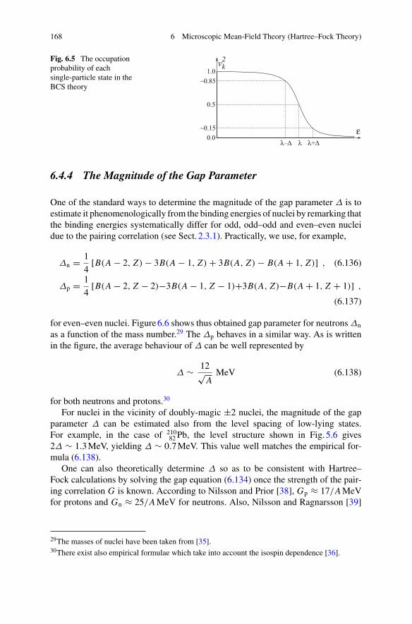
168 6 Microscopic Mean-Field Theory (Hartree–Fock Theory)
Fig. 6.5 The occupationprobability of eachsingle-particle state in theBCS theory
v2k
1.0
0.0
~0.85
~0.15
0.5
λ+Δλλ–Δ
ε
6.4.4 The Magnitude of the Gap Parameter
One of the standard ways to determine the magnitude of the gap parameter Δ is toestimate it phenomenologically from the binding energies of nuclei by remarking thatthe binding energies systematically differ for odd, odd–odd and even–even nucleidue to the pairing correlation (see Sect. 2.3.1). Practically, we use, for example,
Δn = 1
4[B(A − 2, Z) − 3B(A − 1, Z) + 3B(A, Z) − B(A + 1, Z)] , (6.136)
Δp = 1
4[B(A − 2, Z − 2)−3B(A − 1, Z − 1)+3B(A, Z)−B(A + 1, Z + 1)] ,
(6.137)
for even–even nuclei. Figure6.6 shows thus obtained gap parameter for neutrons Δn
as a function of the mass number.29 The Δp behaves in a similar way. As is writtenin the figure, the average behaviour of Δ can be well represented by
Δ ∼ 12√A
MeV (6.138)
for both neutrons and protons.30
For nuclei in the vicinity of doubly-magic ±2 nuclei, the magnitude of the gapparameter Δ can be estimated also from the level spacing of low-lying states.For example, in the case of 210
82 Pb, the level structure shown in Fig. 5.6 gives2Δ ∼ 1.3MeV, yielding Δ ∼ 0.7MeV. This value well matches the empirical for-mula (6.138).
One can also theoretically determine Δ so as to be consistent with Hartree–Fock calculations by solving the gap equation (6.134) once the strength of the pair-ing correlation G is known. According to Nilsson and Prior [38], Gp ≈ 17/AMeVfor protons and Gn ≈ 25/AMeV for neutrons. Also, Nilsson and Ragnarsson [39]
29The masses of nuclei have been taken from [35].30There exist also empirical formulae which take into account the isospin dependence [36].
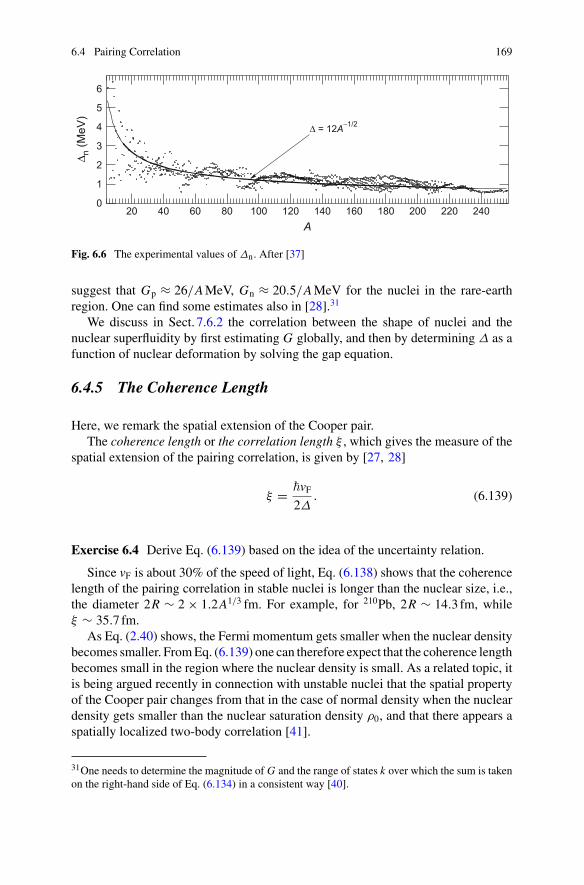
6.4 Pairing Correlation 169
6
5
4
3
2
1
0
Δ n (M
eV)
24022020018016014012010080604020A
Δ = 12A−1/2
Fig. 6.6 The experimental values of Δn. After [37]
suggest that Gp ≈ 26/AMeV, Gn ≈ 20.5/AMeV for the nuclei in the rare-earthregion. One can find some estimates also in [28].31
We discuss in Sect. 7.6.2 the correlation between the shape of nuclei and thenuclear superfluidity by first estimating G globally, and then by determining Δ as afunction of nuclear deformation by solving the gap equation.
6.4.5 The Coherence Length
Here, we remark the spatial extension of the Cooper pair.The coherence length or the correlation length ξ , which gives the measure of the
spatial extension of the pairing correlation, is given by [27, 28]
ξ = �vF2Δ
. (6.139)
Exercise 6.4 Derive Eq. (6.139) based on the idea of the uncertainty relation.
Since vF is about 30% of the speed of light, Eq. (6.138) shows that the coherencelength of the pairing correlation in stable nuclei is longer than the nuclear size, i.e.,the diameter 2R ∼ 2 × 1.2A1/3 fm. For example, for 210Pb, 2R ∼ 14.3 fm, whileξ ∼ 35.7 fm.
As Eq. (2.40) shows, the Fermi momentum gets smaller when the nuclear densitybecomes smaller. FromEq. (6.139) one can therefore expect that the coherence lengthbecomes small in the region where the nuclear density is small. As a related topic, itis being argued recently in connection with unstable nuclei that the spatial propertyof the Cooper pair changes from that in the case of normal density when the nucleardensity gets smaller than the nuclear saturation density ρ0, and that there appears aspatially localized two-body correlation [41].
31One needs to determine the magnitude of G and the range of states k over which the sum is takenon the right-hand side of Eq. (6.134) in a consistent way [40].
170 6 Microscopic Mean-Field Theory (Hartree–Fock Theory)
References
1. G.E. Brown,Unified Theory of Nuclear Models and Forces (North-Holland, Amsterdam, 1967)2. K. Sugimoto, M. Muraoka, Nuclear Physics, Japanese edn. (Kyouritsu, Tokyo, 1998)3. D. Vautherin, D.M. Brink, Phys. Rev. C 5, 626 (1972)4. J.P. Blaizot, Phys. Rep. 64, 171 (1980)5. M. Beiner, H. Flocard, N. Van Giai, P. Quentin. Nucl. Phys. A 238, 29 (1975)6. J. Bartel, P. Quentin, M. Brack, C. Guet, H.-B. Hakansson, Nucl. Phys. A 386, 79 (1982)7. E. Chabanat, P. Bonche, P. Haensel, J. Meyer, R. Schaeffer, Nucl. Phys. A 627, 710 (1997);
635, 231 (1998)8. A. Ono, H. Horiuchi, Prog. Part. Nucl. Phys. 53, 501 (2004)9. H. Ichimura, Statistical Mechanics, Japanese edn. (Shoukabou, 1992)10. R. Kubo, H. Ichimura, T. Usui, N. Hashitsume, Statistical Mechanics–An Advanced Course
with Problems and Solutions (Elsevier, Amsterdam, 1990)11. S. Nishizaki, Y. Yamamoto, T. Takatsuka, Prog. Theor. Phys. 105, 607 (2001); 108, 703 (2002);
Y. Yamamoto, T. Furumoto, N. Yasutake, Th. A. Rijken. Phys. Rev. C 90, 045805 (2014)12. T. Takatsuka, Genshikaku Kenkyu 57, Suppl. 3, 270 (2013); K. Masuda, T. Hatsuda, T. Takat-
suka, Eur. Phys. J. A 52, 65 (2016); I. Vidana. J. Phys. Conf. Ser. 668, 012031 (2016)13. P.J. Siemens, A.S. Jensen, Elements of Nuclei: Many-Body Physics with the Strong Interaction
(Addison and Wesley, California, 1987)14. T. Furuta, A. Ono, Phys. Rev. C 74, 014612 (2006); 79, 014608 (2009)15. T.H.R. Skyrme, Philos. Mag. 1, 1043 (1956); Proc. Phys. Soc. (Lond.) A 70, 433 (1957); Nucl.
Phys. 9, 615 (1958)16. J.P. Jeukenne, A. Lejeune, C. Mahaux, Phys. Rep. 25, 83 (1976); C. Mahaux, P. F. Bortignon,
R.A. Broglia, C.H. Dasso. Phys. Rep. 120, 1 (1985)17. Aage Bohr, Ben R. Mottelson, Nuclear Structure, vol. I (Benjamin, New York, 1969)18. S. Shlomo, J.B. Natowitz, Phys. Lett. B 252, 187 (1990)19. H. Toki, S. Sugimoto, K. Ikeda, Prog. Theor. Phys. 108, 903 (2002)20. B.D. Serot, J.D. Walecka, Adv. Nucl. Phys. 16, 1 (1986)21. P. Ring, Y. K. Gambhir, G. A. Lalazissis, Comp. Phys. Commun. 105, 77 (1997); Y.K. Gambhir,
P. Ring, A. Thimet, Ann. Phys. (N.Y.) 198, 132 (1990)22. W. Greiner, Relativistic Quantum Mechanics (Springer, Berlin, 2000)23. J. Meng, Nucl. Phys. A 635, 3 (1998)24. J.D. Bjorken, S.D. Drell, Relativistic Quantum Mechanics (McGraw-Hill, New York, 1964)25. H. Kurasawa, Butsuri 49, 628 (1994); J.V. Noble. Nucl. Phys. A 329, 354 (1979)26. M.M. Sharma, G. Lalazissis, J. König, P. Ring, Phys. Rev. Lett. 74, 3744 (1995)27. T. Tsuneto, Superconductivity and Superfluidity (Iwanami Modern Physics 17, Japanese edi-
tion) (Iwanami, Tokyo, 1993)28. D.M. Brink, R.A. Broglia, Nuclear Superfluidity-Pairing in Finite Systems (Cambridge Uni-
versity Press, Cambridge, 2005)29. R. Tamagaki, High density nuclear matter (Frontiers of Physics 15, Japanese edition)
(Kyouritsu, 1986); Prog. Theor. Phys. 44, 905 (1970)30. W. Greiner, J.A. Maruhn, Nuclear Models (Springer, Berlin, 1995)31. K. Dietrich, H.J. Mang, J.H. Pradal, Phys. Rev. 135, B22 (1964)32. H.J. Lipkin, Ann. Phys. (N.Y.) 9, 272 (1960); 12, 452 (1961)33. Y. Nogami, Phys. Rev. 134, B313 (1964)34. P. Ring, P. Schuck, The Nuclear Many-Body Problem (Springer, Berlin, 1980)35. G. Audi, A.H. Wapstra, C. Thibault, Nucl. Phys. A 729, 337 (2003)36. D.G. Madland, J.R. Nix, Nucl. Phys. A 476, 1 (1988)37. H. Koura, private communication38. S.G. Nilsson, O. Prior, Mat. Fys. Medd. Dan. Vid. Selsk. 32, 16 (1961)39. S.G. Nilsson, I. Ragnarsson, Shapes and Shells in Nuclear Structure (Cambridge University
Press, Cambridge, 1995)40. A. Bulgac, Y. Yu, Phys. Rev. Lett. 88, 042504 (2002)41. M. Matsuo, Phys. Rev. C 73, 044309 (2006)
Chapter 7The Shapes of Nuclei
Abstract The nucleus behaves like a liquid drop as the mass formula and thesaturation of density imply. However, a significant difference from the classical liquiddrop, which is always spherical in order to make the energy by surface tension min-imum, is that many nuclei are deformed except for those near the closed shells. Theshape of nuclei is one of the central research subjects of nuclear structure togetherwith the size of nuclei. The shape of nuclei is intimately related to the collectiveexcitations of nuclei, and also strongly affects nuclear reactions including heavy-ion fusion reactions (see Balantekin and Takigawa, Rev. Mod. Phys. 70, 77 (1998);Dasgupta et al., Annu. Rev. Nucl. Part. Sci. 48, 401 (1998); Hagino et al., Comput.Phys. Commun. 123, 143 (1999); Esbensen, Nucl. Phys. A 352, 147 (1981); Haginoand Takigawa, Butsuri 57, 588 (2002); Hagino and Takigawa, Prog. Theor. Phys. 128,1001 (2012) [1–6]). In this chapter we describe several basic concepts concerningthe shape of nuclei.
7.1 The Observables Relevant to the Nuclear Shape:Multipole Moments and the Excitation Spectrum
As pointed out in Chap. 4, the magnitude of the electric quadrupole moment providesdirect information on the nuclear shape, more precisely, on whether the distributionof protons inside the nucleus is spherical or deformed. We learn in Sect. 8.3 thatthe electromagnetic transitions give related valuable information on the shape ofthe nucleus. Figures 7.1a and 7.1b show the energy levels of 166
68 Er and 16768 Er in the
vicinity of the ground state taken from [7] (the excitation energies are in keV).The level structure of 166
68 Er resembles that for 210Pb and 210Po shown in Fig. 5.6in the sense that the I π = 0+, 2+, 4+, 6+, 8+ levels appear in low energy region inthis order. However, it significantly differs in that the level spacing increases withincreasing angular momentum I . The level spacing well agrees with the spectrumEI = �
2 I (I + 1)/2I , I being the moment of inertia, of the rotational motion,which is a characteristic collective motion of statically deformed nuclei. The levelstructure of 167
68 Er is similar. Figures 7.1a and 7.1b therefore suggest that these nucleiare deformed nuclei.
© Springer Japan 2017N. Takigawa and K. Washiyama, Fundamentals of Nuclear Physics,DOI 10.1007/978-4-431-55378-6_7
171
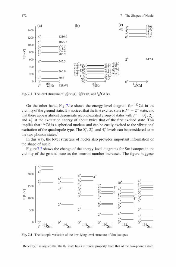
172 7 The Shapes of Nuclei
0
200
400
600
800
1000
1200
1400
E [
keV
](a) (b) (c)
166Er68Jπ E [keV]0+2+
4+
6+
2+3+8+4+5+
6+
080.6
265.0
545.5
785.9859.4911.2956.21075.3
1216.0
167Er687/2+9/2+11/2+1/2– 3/2–5/2–13/2+5/2– 7/2–7/2–15/2+9/2–
079.3178.0 207.8264.9 281.6293.7 346.6412.3 430.0432.4 442.0
112Cd480+
2+
0+2+4+(0)+ 2+
0
617.4
12231313141514291468
Fig. 7.1 The level structure of 16668 Er (a), 167
68 Er (b) and 11248 Cd (c)
On the other hand, Fig. 7.1c shows the energy-level diagram for 112Cd in thevicinity of the ground state. It is noticed that the first excited state is I π = 2+ state, andthat there appear almost degenerate second excited group of states with I π = 0+
2 , 2+2 ,
and 4+1 at the excitation energy of about twice that of the first excited state. This
implies that 112Cd is a spherical nucleus and can be easily excited to the vibrationalexcitation of the quadrupole type. The 0+
2 , 2+2 , and 4+
1 levels can be considered to bethe two phonon states.1
In this way, the level structure of nuclei also provides important information onthe shape of nuclei.
Figure 7.2 shows the change of the energy-level diagrams for Sm isotopes in thevicinity of the ground state as the neutron number increases. The figure suggests
0
500
1000
1500
2000
E [
keV
]
144Sm62Jπ0+
0+2+
4+6+
146Sm0+
2+
4+
2+6+
148Sm0+
2+
0+4+0+2+2+4+ 4+6+
150Sm0+
2+
0+4+2+2+ 0+6+2+ 4+3+
152Sm0+2+
4+
0+6+2+4+2+ 0+8+3+4+
10+
154Sm0+2+4+
6+
8+0+2+0+4+2+3+4+
Fig. 7.2 The isotopic variation of the low-lying level structure of Sm isotopes
1Recently, it is argued that the 0+2 state has a different property from that of the two-phonon state.
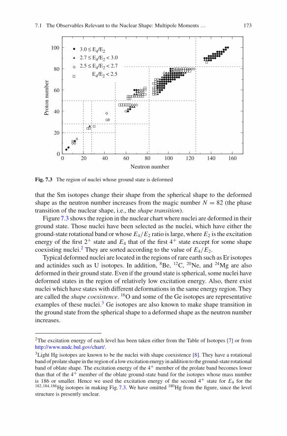
7.1 The Observables Relevant to the Nuclear Shape: Multipole Moments … 173
0
20
40
60
80
100
0 20 40 60 80 100 120 140 160
Prot
on num
ber
Neutron number
3.0 ≤ E4/E2
2.7 ≤ E4/E2 < 3.0
2.5 ≤ E4/E2 < 2.7
E4/E2 < 2.5
Fig. 7.3 The region of nuclei whose ground state is deformed
that the Sm isotopes change their shape from the spherical shape to the deformedshape as the neutron number increases from the magic number N = 82 (the phasetransition of the nuclear shape, i.e., the shape transition).
Figure 7.3 shows the region in the nuclear chart where nuclei are deformed in theirground state. Those nuclei have been selected as the nuclei, which have either theground-state rotational band or whose E4/E2 ratio is large, where E2 is the excitationenergy of the first 2+ state and E4 that of the first 4+ state except for some shapecoexisting nuclei.2 They are sorted according to the value of E4/E2.
Typical deformed nuclei are located in the regions of rare earth such as Er isotopesand actinides such as U isotopes. In addition, 8Be, 12C, 20Ne, and 24Mg are alsodeformed in their ground state. Even if the ground state is spherical, some nuclei havedeformed states in the region of relatively low excitation energy. Also, there existnuclei which have states with different deformations in the same energy region. Theyare called the shape coexistence. 16O and some of the Ge isotopes are representativeexamples of these nuclei.3 Ge isotopes are also known to make shape transition inthe ground state from the spherical shape to a deformed shape as the neutron numberincreases.
2The excitation energy of each level has been taken either from the Table of Isotopes [7] or fromhttp://www.nndc.bnl.gov/chart/.3Light Hg isotopes are known to be the nuclei with shape coexistence [8]. They have a rotationalband of prolate shape in the region of a low excitation energy in addition to the ground-state rotationalband of oblate shape. The excitation energy of the 4+ member of the prolate band becomes lowerthan that of the 4+ member of the oblate ground-state band for the isotopes whose mass numberis 186 or smaller. Hence we used the excitation energy of the second 4+ state for E4 for the182,184,186Hg isotopes in making Fig. 7.3. We have omitted 180Hg from the figure, since the levelstructure is presently unclear.
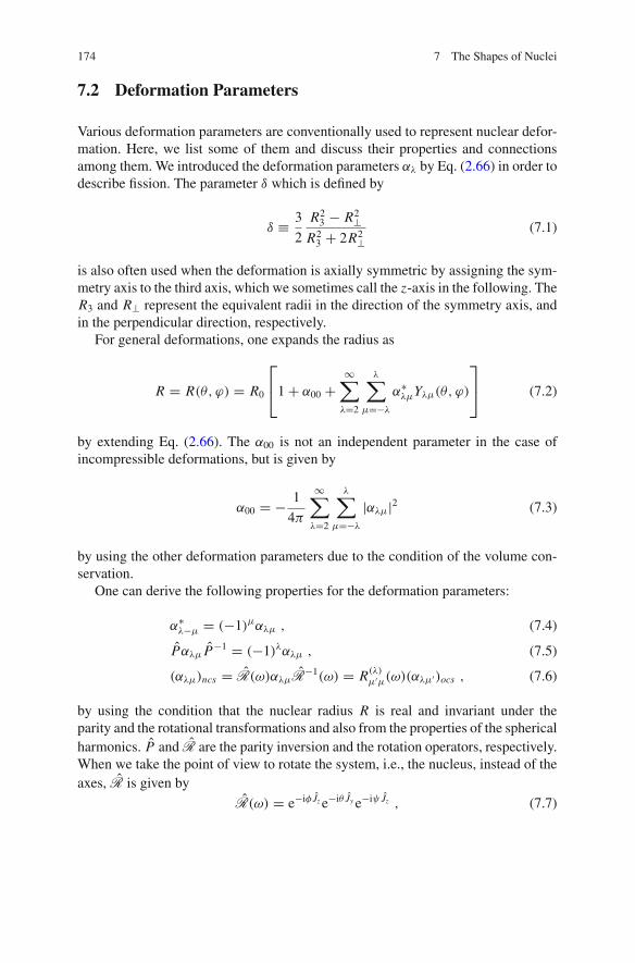
174 7 The Shapes of Nuclei
7.2 Deformation Parameters
Various deformation parameters are conventionally used to represent nuclear defor-mation. Here, we list some of them and discuss their properties and connectionsamong them. We introduced the deformation parameters αλ by Eq. (2.66) in order todescribe fission. The parameter δ which is defined by
δ ≡ 3
2
R23 − R2
⊥R2
3 + 2R2⊥
(7.1)
is also often used when the deformation is axially symmetric by assigning the sym-metry axis to the third axis, which we sometimes call the z-axis in the following. TheR3 and R⊥ represent the equivalent radii in the direction of the symmetry axis, andin the perpendicular direction, respectively.
For general deformations, one expands the radius as
R = R(θ, ϕ) = R0
⎡⎣1 + α00 +
∞∑λ=2
λ∑μ=−λ
α∗λμYλμ(θ, ϕ)
⎤⎦ (7.2)
by extending Eq. (2.66). The α00 is not an independent parameter in the case ofincompressible deformations, but is given by
α00 = − 1
4π
∞∑λ=2
λ∑μ=−λ
|αλμ|2 (7.3)
by using the other deformation parameters due to the condition of the volume con-servation.
One can derive the following properties for the deformation parameters:
α∗λ−μ = (−1)μαλμ , (7.4)
Pαλμ P−1 = (−1)λαλμ , (7.5)
(αλμ)ncs = R(ω)αλμR−1(ω) = R(λ)
μ′μ(ω)(αλμ′)ocs , (7.6)
by using the condition that the nuclear radius R is real and invariant under theparity and the rotational transformations and also from the properties of the sphericalharmonics. P and R are the parity inversion and the rotation operators, respectively.When we take the point of view to rotate the system, i.e., the nucleus, instead of theaxes, R is given by
R(ω) = e−iφ Jz e−iθ Jy e−iψ Jz , (7.7)
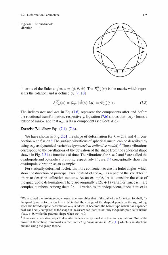
7.2 Deformation Parameters 175
Fig. 7.4 The quadrupolevibration
in terms of the Euler angles ω = (φ, θ, ψ). The R(λ)μ′μ(ω) is the matrix which repre-
sents the rotation, and is defined by [9, 10]
R(λ)μ′μ(ω) ≡ 〈λμ′|R(ω)|λμ〉 = Dλ ∗
μ′μ(ω) . (7.8)
The indices ncs and ocs in Eq. (7.6) represent the components after and beforethe rotational transformation, respectively. Equation (7.6) shows that {αλμ} forms atensor of rank-λ and that αλμ is its μ component (see Sect. A.6).
Exercise 7.1 Show Eqs. (7.4)–(7.6).
We have shown in Fig. 2.21 the shape of deformation for λ = 2, 3 and 4 in con-nection with fission.4 The surface vibrations of spherical nuclei can be described byusing αλμ as dynamical variables (geometrical collective model).5 Those vibrationscorrespond to the oscillations of the deviation of the shape from the spherical shapeshown in Fig. 2.21 as functions of time. The vibrations for λ = 2 and 3 are called thequadrupole and octupole vibrations, respectively. Figure. 7.4 conceptually shows thequadrupole vibration as an example.
For statically deformed nuclei, it is more convenient to use the Euler angles, whichshow the direction of principal axes, instead of the αλμ as a part of the variables inorder to describe collective motions. As an example, let us consider the case ofthe quadrupole deformation. There are originally 2(2λ + 1) variables, since αλμ arecomplex numbers. Among them 2λ + 1 variables are independent, since there exist
4We assumed the prolate type, whose shape resembles that of the ball of the American football, forthe quadrupole deformation λ = 2. Note that the change of the shape depends on the sign of α40when the hexadecapole deformation α40 is added. It becomes the barrel type which has expandedpeaks and belly compared to the shape in the case when there exists only the quadrupole deformationif α40 > 0, while the peanuts shape when α40 < 0.5There exist alternative ways to describe nuclear energy level structure and excitations. One of thepowerful theoretical frameworks is the interacting boson model (IBM) [11] which is an algebraicmethod using the group theory.
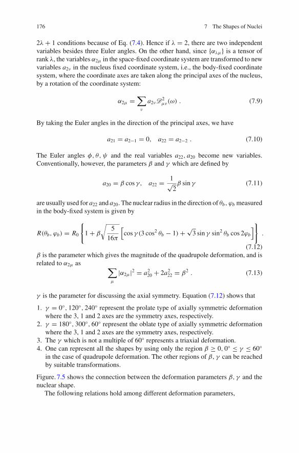
176 7 The Shapes of Nuclei
2λ + 1 conditions because of Eq. (7.4). Hence if λ = 2, there are two independentvariables besides three Euler angles. On the other hand, since {αλμ} is a tensor ofrank λ, the variables α2μ in the space-fixed coordinate system are transformed to newvariables a2ν in the nucleus fixed coordinate system, i.e., the body-fixed coordinatesystem, where the coordinate axes are taken along the principal axes of the nucleus,by a rotation of the coordinate system:
α2μ =∑
ν
a2νD2μν(ω) . (7.9)
By taking the Euler angles in the direction of the principal axes, we have
a21 = a2−1 = 0, a22 = a2−2 . (7.10)
The Euler angles φ, θ, ψ and the real variables a22, a20 become new variables.Conventionally, however, the parameters β and γ which are defined by
a20 = β cos γ, a22 = 1√2β sin γ (7.11)
are usually used for a22 and a20. The nuclear radius in the direction of θb, ϕb measuredin the body-fixed system is given by
R(θb, ϕb) = R0
{1 + β
√5
16π
[cos γ (3 cos2 θb − 1) + √
3 sin γ sin2 θb cos 2ϕb
]}.
(7.12)β is the parameter which gives the magnitude of the quadrupole deformation, and isrelated to α2μ as ∑
μ
|α2μ|2 = a220 + 2a2
22 = β2 . (7.13)
γ is the parameter for discussing the axial symmetry. Equation (7.12) shows that
1. γ = 0◦, 120◦, 240◦ represent the prolate type of axially symmetric deformationwhere the 3, 1 and 2 axes are the symmetry axes, respectively.
2. γ = 180◦, 300◦, 60◦ represent the oblate type of axially symmetric deformationwhere the 3, 1 and 2 axes are the symmetry axes, respectively.
3. The γ which is not a multiple of 60◦ represents a triaxial deformation.4. One can represent all the shapes by using only the region β ≥ 0, 0◦ ≤ γ ≤ 60◦
in the case of quadrupole deformation. The other regions of β, γ can be reachedby suitable transformations.
Figure. 7.5 shows the connection between the deformation parameters β, γ and thenuclear shape.
The following relations hold among different deformation parameters,
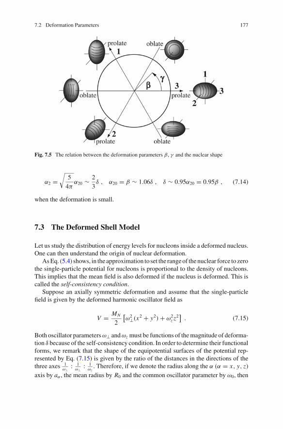
7.2 Deformation Parameters 177
Fig. 7.5 The relation between the deformation parameters β, γ and the nuclear shape
α2 =√
5
4πα20 ∼ 2
3δ , α20 = β ∼ 1.06δ , δ ∼ 0.95α20 = 0.95β , (7.14)
when the deformation is small.
7.3 The Deformed Shell Model
Let us study the distribution of energy levels for nucleons inside a deformed nucleus.One can then understand the origin of nuclear deformation.
As Eq. (5.4) shows, in the approximation to set the range of the nuclear force to zerothe single-particle potential for nucleons is proportional to the density of nucleons.This implies that the mean field is also deformed if the nucleus is deformed. This iscalled the self-consistency condition.
Suppose an axially symmetric deformation and assume that the single-particlefield is given by the deformed harmonic oscillator field as
V = MN
2
[ω2
⊥(x2 + y2) + ω2z z
2]
. (7.15)
Both oscillator parameters ω⊥ and ωz must be functions of the magnitude of deforma-tion δ because of the self-consistency condition. In order to determine their functionalforms, we remark that the shape of the equipotential surfaces of the potential rep-resented by Eq. (7.15) is given by the ratio of the distances in the directions of thethree axes 1
ω⊥ : 1ω⊥ : 1
ωz. Therefore, if we denote the radius along the α (α = x, y, z)
axis by aα , the mean radius by R0 and the common oscillator parameter by ω0, then
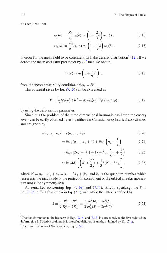
178 7 The Shapes of Nuclei
it is required that
ωz(δ) = R0
azω0(δ) ∼
(1 − 2
3δ
)ω0(δ) , (7.16)
ω⊥(δ) = R0
a⊥ω0(δ) ∼
(1 + 1
3δ
)ω0(δ) , (7.17)
in order for the mean field to be consistent with the density distribution6 [12]. If wedenote the mean oscillator parameter by ω,7 then we obtain
ω0(δ) ∼ ω
(1 + 1
9δ2
), (7.18)
from the incompressibility condition ω2⊥ωz = ω3.
The potential given by Eq. (7.15) can be expressed as
V = 1
2MNω2
0(δ)r2 − MNω2
0(δ)r2βY20(θ, φ) (7.19)
by using the deformation parameter.Since it is the problem of the three-dimensional harmonic oscillator, the energy
levels can be easily obtained by using either the Cartesian or cylindrical coordinates,and are given by
ε(nx , ny, nz) = ε(nz, nρ, k�) (7.20)
= �ω⊥(nx + ny + 1) + �ωz
(nz + 1
2
)(7.21)
= �ω⊥(2nρ + |k�| + 1) + �ωz
(nz + 1
2
)(7.22)
∼ �ω0(δ)
[(N + 3
2
)+ 1
3δ(N − 3nz)
], (7.23)
where N = nx + ny + nz = nz + 2nρ + |k�| and k� is the quantum number whichrepresents the magnitude of the projection component of the orbital angular momen-tum along the symmetry axis.
As remarked concerning Eqs. (7.16) and (7.17), strictly speaking, the δ inEq. (7.23) differs from the δ in Eq. (7.1), and while the latter is defined by
δ ≡ 3
2
R2z − R2
⊥R2z + 2R2
⊥= 3
2
ω2⊥(δ) − ω2
z (δ)
ω2⊥(δ) + 2ω2
z (δ), (7.24)
6The transformation to the last term in Eqs. (7.16) and (7.17) is correct only to the first order of thedeformation δ. Strictly speaking, it is therefore different from the δ defined by Eq. (7.1).7The rough estimate of �ω is given by Eq. (5.52).
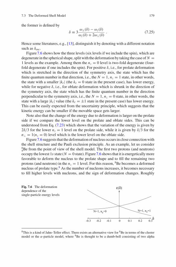
7.3 The Deformed Shell Model 179
the former is defined by
δ ≡ 3ω⊥(δ) − ωz(δ)
ωz(δ) + 2ω⊥(δ). (7.25)
Hence some literatures, e.g., [13], distinguish it by denoting with a different notationsuch as δosc.
Figure 7.6 shows how the three levels (six levels if we include the spin), which aredegenerate in the spherical shape, split with the deformation by taking the case of N =1 levels as the example. Among them the nz = 0 level is two-fold degenerate (four-fold degenerate if one includes the spin). For positive δ, i.e., for prolate deformationwhich is stretched in the direction of the symmetry axis, the state which has thefinite quantum number in that direction, i.e., the N = 1, nz = 1 state, in other words,the state with a smaller |k�| (the k� = 0 state in the present case), has lower energy,while for negative δ, i.e., for oblate deformation which is shrunk in the direction ofthe symmetry axis, the state which has the finite quantum number in the directionperpendicular to the symmetry axis, i.e., the N = 1, nz = 0 state, in other words, thestate with a large |k�| value (the k� = ±1 state in the present case) has lower energy.This can be easily expected from the uncertainty principle, which suggests that thekinetic energy can be smaller if the movable space gets larger.
Note also that the change of the energy due to deformation is larger on the prolateside if we compare the lower level on the prolate and oblate sides. This can beunderstood from Eq. (7.23) which shows that the variation of the energy is given by2δ/3 for the lower nz = 1 level on the prolate side, while it is given by δ/3 for then⊥ = 1(nz = 0) level which is the lower level on the oblate side.
Figure 7.6 suggests that the deformation of nucleus occurs in close connection withthe shell structure and the Pauli exclusion principle. As an example, let us consider84Be from the point of view of the shell model. The first two protons (and neutrons)occupy the lowest 1s state (N = 0 state). Figure 7.6 shows that it is energetically morefavorable to deform the nucleus to the prolate shape and to fill the remaining twoprotons (and neutrons) in the nz = 1 level. For this reason, 8Be becomes a deformednucleus of prolate type.8 As the number of nucleons increases, it becomes necessaryto fill higher levels with nucleons, and the sign of deformation changes. Roughly
Fig. 7.6 The deformationdependence of thesingle-particle energy levels
-0.3 -0.2 -0.1 0 0.1 0.2 0.3
ε(δ)
δ
N=1, nz=1N=1, nz=0
8This is a kind of Jahn–Teller effect. There exists an alternative view for 8Be in terms of the clustermodel or the α-particle model, where 8Be is thought to be a dumb-bell consisting of two alpha
180 7 The Shapes of Nuclei
speaking, it can be expected that the nuclei which belong to the beginning of a majorshell have prolate deformation, while those towards the end of the shell oblate. Forexample, in the case of N = 1 shell, i.e., the 1p shell, 8Be, which belongs to thefirst half, has a prolate deformation, while 12C, which belongs to the last half, has anoblate shape. However, in reality most of the deformed nuclei are prolate, and thosewhich are oblate in their ground state are limited to 12C and small number of nucleisuch as some of the Hg isotopes, which we mentioned in connection with Fig. 7.3and will discuss again in Sect. 7.6.2.
7.4 Nucleon Energy Levels in a Deformed One-Body Field:Nilsson Levels
The spin–orbit coupling is indispensable in order to discuss real nuclei. Also, theradial dependence of the harmonic oscillator type is unrealistic. Hence we assumethat the Hamiltonian for nucleons is given by
h = − �2
2MNΔ + MN
2ω2
⊥(x2 + y2) + MN
2ω2z z
2 + C� · s + D�2 (7.26)
by extending the deformed harmonic oscillator model introduced in the previoussection. The �2 term has been introduced in order to effectively improve the harmonicoscillator model so as to yield the level structure for the realistic radial dependenceof the Woods–Saxon type, and is designed in such a way that the states with largerorbital angular momentum feel stronger attraction (see Fig. 5.1). The single-particlelevels obtained by Eq. (7.26) are called Nilsson levels or Nilsson diagram or Nilssonscheme, since this model was proposed by Nilsson [14] for the first time.
The Nilsson levels and the associated wave functions can be obtained by diago-nalizing the Hamiltonian given by Eq. (7.26) by using a suitable complete set as theexpansion basis. For example, using the wave functions of the deformed shell modelconsidered in the previous section |α〉 = |Nnzk�Ω〉 as the basis, we expand the wavefunction as
|φi=Nnzk�Ω〉 =∑
α
Ciα|α〉 , (7.27)
and determine the expansion coefficients Ciα and the corresponding single-particleenergy εi by diagonalizing h. Ω = k� + ms is the magnitude of the projection com-ponent of the total angular momentum along the symmetry axis, where ms is themagnitude of the projection component of the spin along the symmetry axis.
Figure 7.7 shows an example of the Nilsson levels. The followings are someremarks concerning the Nilsson levels.
particles. However, the overlap between the wave functions of the shell model and of the clustermodel is fairly large.
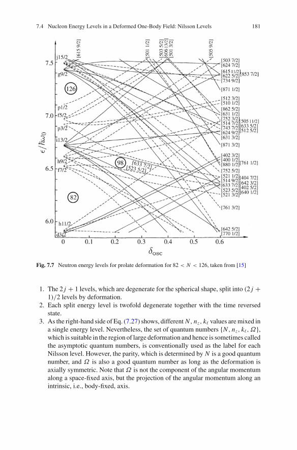
7.4 Nucleon Energy Levels in a Deformed One-Body Field: Nilsson Levels 181
Fig. 7.7 Neutron energy levels for prolate deformation for 82 < N < 126, taken from [15]
1. The 2 j + 1 levels, which are degenerate for the spherical shape, split into (2 j +1)/2 levels by deformation.
2. Each split energy level is twofold degenerate together with the time reversedstate.
3. As the right-hand side of Eq. (7.27) shows, different N , nz, k� values are mixed ina single energy level. Nevertheless, the set of quantum numbers {N , nz, k�,Ω},which is suitable in the region of large deformation and hence is sometimes calledthe asymptotic quantum numbers, is conventionally used as the label for eachNilsson level. However, the parity, which is determined by N is a good quantumnumber, and Ω is also a good quantum number as long as the deformation isaxially symmetric. Note that Ω is not the component of the angular momentumalong a space-fixed axis, but the projection of the angular momentum along anintrinsic, i.e., body-fixed, axis.
182 7 The Shapes of Nuclei
4. Roughly speaking, for prolate deformation (δ > 0), the states with small Ω gainnegative energy by deformation and the amount of the gain is larger for smallerΩ . The shift of energy by deformation gradually changes with Ω , and turns to bepositive for states with large values of Ω . The trend of the effect of deformationis opposite for oblate deformation. However, the effect of deformation is morecomplex for oblate deformation.
7.5 The Spin and Parity of the Ground State of DeformedOdd Nuclei
One can speculate the spin and parity of the ground state of deformed odd nuclei byreferring to the Nilsson diagram.
Consider 16768 Er as an example. From the analysis of the inelastic scattering of α
particles, i.e., (α, α′) scattering, it is known that the quadrupole deformation of 16668 Er
is β2 = 0.276 [16]. If the quadrupole moment of 16768 Er is assumed to be nearly equal,
then the spin of the ground state of 16768 Er is predicted to be 7/2 from the Ω value of
the 99th energy level for neutrons in Fig. 7.7. Also, the parity is expected to be plus,since this level results from the split of the i13/2 level. These predictions agree withthe experimental results shown in Fig. 7.1b.
7.6 Theoretical Prediction of Nuclear Shape
There are various theoretical methods to confirm nuclear shapes determined or pre-dicted by experimental data or to predict unknown nuclear shapes. Here, we explaintwo standard methods which determine the nuclear shape based on the calculationof binding energies.
7.6.1 The Strutinsky Method: Macroscopic–MicroscopicMethod
One of the methods is the method which reconciles the liquid-drop model and theshell model. It is called either the macroscopic–microscopic method or the Strutinskyshell correction method after the name of the inventor [17]. This method gives also thebinding energy of nuclei and the potential surface for fission with high accuracy [18].
Leaving the detailed explanation of the method to other books [19], here wemention the basic concept of this method.
As we see in Fig. 2.6, the binding energy consists of the part ELDM which smoothlydepends on the mass number and can be well explained by the liquid-drop model,
7.6 Theoretical Prediction of Nuclear Shape 183
and the part which deviates from it and oscillates, i.e., detailed structure;
Etot = ELDM + Eosc . (7.28)
The oscillating part arises because the distribution of single-particle energy lev-els deviates from the average level density and is non-uniform reflecting the shellstructure.
In the Strutinsky method, the part which depends smoothly on the mass number isestimated macroscopically based on the liquid-drop model, while the oscillating partEosc as the difference between the energy microscopically calculated by the shellmodel and the mean energy Esh calculated by introducing the average level density
Eosc = Esh − Esh . (7.29)
If we denote the accurate or shell model level density by g(ε), the average leveldensity by g(ε), the Fermi energy by λ, and the Fermi energy when the average leveldensity is used by λ, then
g(ε) =A∑
i=1
δ(ε − εi ) , (7.30)
Esh =A∑
i=1
εi =∫ λ
−∞εg(ε)dε , (7.31)
Esh =∫ λ
−∞εg(ε)dε , (7.32)
A =∫ λ
−∞g(ε)dε =
∫ λ
−∞g(ε)dε , (7.33)
where we denote the mass number by A.The folding method,
g(ε) = 1
γ
∫ ∞
−∞g(ε′) f
(ε′ − ε
γ
)dε′ , (7.34)
where f is a Gaussian, whose width γ is of the order of �ω0, is a candidate of themethod to introduce the average level density. However, one must be sure that theresult does not change when the averaging procedure is repeated [19].
Incidentally, Eq. (7.29) is revised as
Eosc = Esh − Esh + Epair − Epair (7.35)
if the pairing energy is taken into account in the BCS method.
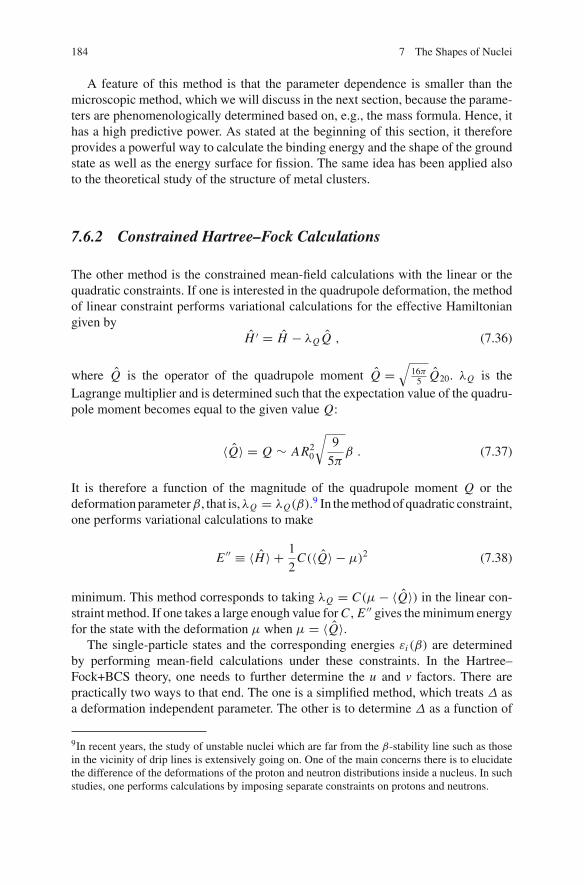
184 7 The Shapes of Nuclei
A feature of this method is that the parameter dependence is smaller than themicroscopic method, which we will discuss in the next section, because the parame-ters are phenomenologically determined based on, e.g., the mass formula. Hence, ithas a high predictive power. As stated at the beginning of this section, it thereforeprovides a powerful way to calculate the binding energy and the shape of the groundstate as well as the energy surface for fission. The same idea has been applied alsoto the theoretical study of the structure of metal clusters.
7.6.2 Constrained Hartree–Fock Calculations
The other method is the constrained mean-field calculations with the linear or thequadratic constraints. If one is interested in the quadrupole deformation, the methodof linear constraint performs variational calculations for the effective Hamiltoniangiven by
H ′ = H − λQ Q , (7.36)
where Q is the operator of the quadrupole moment Q =√
16π5 Q20. λQ is the
Lagrange multiplier and is determined such that the expectation value of the quadru-pole moment becomes equal to the given value Q:
〈Q〉 = Q ∼ AR20
√9
5πβ . (7.37)
It is therefore a function of the magnitude of the quadrupole moment Q or thedeformation parameterβ, that is,λQ = λQ(β).9 In the method of quadratic constraint,one performs variational calculations to make
E ′′ ≡ 〈H〉 + 1
2C(〈Q〉 − μ)2 (7.38)
minimum. This method corresponds to taking λQ = C(μ − 〈Q〉) in the linear con-straint method. If one takes a large enough value forC , E ′′ gives the minimum energyfor the state with the deformation μ when μ = 〈Q〉.
The single-particle states and the corresponding energies εi (β) are determinedby performing mean-field calculations under these constraints. In the Hartree–Fock+BCS theory, one needs to further determine the u and v factors. There arepractically two ways to that end. The one is a simplified method, which treats Δ asa deformation independent parameter. The other is to determine Δ as a function of
9In recent years, the study of unstable nuclei which are far from the β-stability line such as thosein the vicinity of drip lines is extensively going on. One of the main concerns there is to elucidatethe difference of the deformations of the proton and neutron distributions inside a nucleus. In suchstudies, one performs calculations by imposing separate constraints on protons and neutrons.
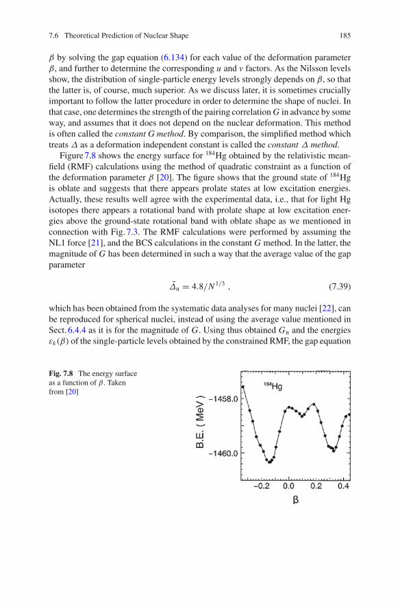
7.6 Theoretical Prediction of Nuclear Shape 185
β by solving the gap equation (6.134) for each value of the deformation parameterβ, and further to determine the corresponding u and v factors. As the Nilsson levelsshow, the distribution of single-particle energy levels strongly depends on β, so thatthe latter is, of course, much superior. As we discuss later, it is sometimes cruciallyimportant to follow the latter procedure in order to determine the shape of nuclei. Inthat case, one determines the strength of the pairing correlation G in advance by someway, and assumes that it does not depend on the nuclear deformation. This methodis often called the constant G method. By comparison, the simplified method whichtreats Δ as a deformation independent constant is called the constant Δ method.
Figure 7.8 shows the energy surface for 184Hg obtained by the relativistic mean-field (RMF) calculations using the method of quadratic constraint as a function ofthe deformation parameter β [20]. The figure shows that the ground state of 184Hgis oblate and suggests that there appears prolate states at low excitation energies.Actually, these results well agree with the experimental data, i.e., that for light Hgisotopes there appears a rotational band with prolate shape at low excitation ener-gies above the ground-state rotational band with oblate shape as we mentioned inconnection with Fig. 7.3. The RMF calculations were performed by assuming theNL1 force [21], and the BCS calculations in the constant G method. In the latter, themagnitude of G has been determined in such a way that the average value of the gapparameter
Δn = 4.8/N 1/3 , (7.39)
which has been obtained from the systematic data analyses for many nuclei [22], canbe reproduced for spherical nuclei, instead of using the average value mentioned inSect. 6.4.4 as it is for the magnitude of G. Using thus obtained Gn and the energiesεk(β) of the single-particle levels obtained by the constrained RMF, the gap equation
Fig. 7.8 The energy surfaceas a function of β. Takenfrom [20]
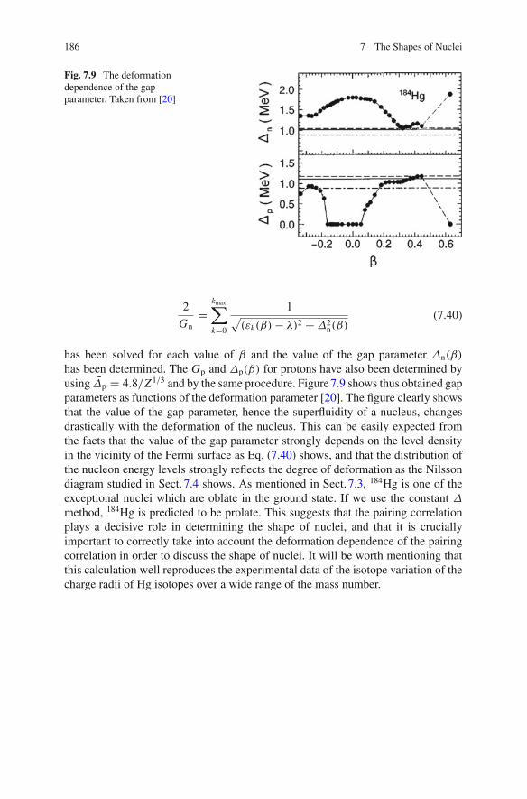
186 7 The Shapes of Nuclei
Fig. 7.9 The deformationdependence of the gapparameter. Taken from [20]
2
Gn=
kmax∑k=0
1√(εk(β) − λ)2 + Δ2
n(β)(7.40)
has been solved for each value of β and the value of the gap parameter Δn(β)
has been determined. The Gp and Δp(β) for protons have also been determined byusing Δp = 4.8/Z1/3 and by the same procedure. Figure 7.9 shows thus obtained gapparameters as functions of the deformation parameter [20]. The figure clearly showsthat the value of the gap parameter, hence the superfluidity of a nucleus, changesdrastically with the deformation of the nucleus. This can be easily expected fromthe facts that the value of the gap parameter strongly depends on the level densityin the vicinity of the Fermi surface as Eq. (7.40) shows, and that the distribution ofthe nucleon energy levels strongly reflects the degree of deformation as the Nilssondiagram studied in Sect. 7.4 shows. As mentioned in Sect. 7.3, 184Hg is one of theexceptional nuclei which are oblate in the ground state. If we use the constant Δ
method, 184Hg is predicted to be prolate. This suggests that the pairing correlationplays a decisive role in determining the shape of nuclei, and that it is cruciallyimportant to correctly take into account the deformation dependence of the pairingcorrelation in order to discuss the shape of nuclei. It will be worth mentioning thatthis calculation well reproduces the experimental data of the isotope variation of thecharge radii of Hg isotopes over a wide range of the mass number.
7.7 Column: Superdeformed States 187
7.7 Column: Superdeformed StatesThe amount of deformation of rare-earth nuclei and actinides in their groundstates is about δ ∼ 0.3. By comparison, the deformation of light deformed nucleisuch as 8Be is large.
Today, many states with large deformation have been found in the excitationenergy region in the medium-mass and heavy nuclei as well. They are calledsuperdeformed states and superdeformed rotational bands built on them, andhave been extensively studied together with high spin states [23].
The fission isomers mentioned in Sect. 2.3.3 are typical examples of superde-formed states. Figure 7.10 shows the distribution of superdeformed bands andfission isomers on the nuclear chart.
We learnt in Sect. 7.3 that the deformation of nucleus is intimately related tothe shell structure of single-particle levels. In this connection, Fig. 7.11 showsthe distribution of single-particle energy levels in the deformed shell model. Thefigure shows that there appears a distinct shell structure, i.e., the degeneracy oflevels, similar to that for δ = 0, when the ratio between the long and short axesRz : R⊥ becomes, e.g., 2:1. This happens because in that case the ratio of themagnitudes of the energy quanta in the direction parallel to the symmetry axisand in the perpendicular direction �ωz : �ω⊥ becomes 1:2 due to the consistencycondition between the potential for nucleons and the nucleon density. In thiscase, the deformation δ(SD) of the superdeformed state becomes δ(SD)
osc = 0.6 interms of δosc defined by Eq. (7.25).
Fig. 7.10 The distribution of superdeformed states, taken from [24]
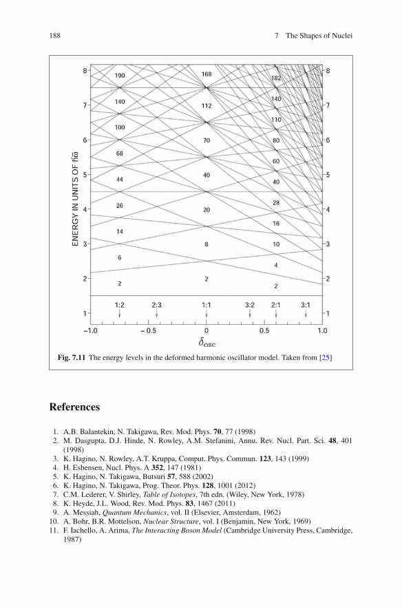
188 7 The Shapes of Nuclei
Fig. 7.11 The energy levels in the deformed harmonic oscillator model. Taken from [25]
References
1. A.B. Balantekin, N. Takigawa, Rev. Mod. Phys. 70, 77 (1998)2. M. Dasgupta, D.J. Hinde, N. Rowley, A.M. Stefanini, Annu. Rev. Nucl. Part. Sci. 48, 401
(1998)3. K. Hagino, N. Rowley, A.T. Kruppa, Comput. Phys. Commun. 123, 143 (1999)4. H. Esbensen, Nucl. Phys. A 352, 147 (1981)5. K. Hagino, N. Takigawa, Butsuri 57, 588 (2002)6. K. Hagino, N. Takigawa, Prog. Theor. Phys. 128, 1001 (2012)7. C.M. Lederer, V. Shirley, Table of Isotopes, 7th edn. (Wiley, New York, 1978)8. K. Heyde, J.L. Wood, Rev. Mod. Phys. 83, 1467 (2011)9. A. Messiah, Quantum Mechanics, vol. II (Elsevier, Amsterdam, 1962)
10. A. Bohr, B.R. Mottelson, Nuclear Structure, vol. I (Benjamin, New York, 1969)11. F. Iachello, A. Arima, The Interacting Boson Model (Cambridge University Press, Cambridge,
1987)
References 189
12. G.E. Brown,Unified Theory of NuclearModels and Forces (North-Holland, Amsterdam, 1967)13. A. Bohr, B.R. Mottelson, Nuclear Structure, vol. II (Benjamin, New York, 1975)14. S.G. Nilsson, Mat. Fys. Medd. Dan. Vid. Selsk. 29(16), (1955)15. C. Gustafson, I.L. Lam, B. Nilsson, S.G. Nilsson, Ark. Fys. 36, 613 (1967)16. D.L. Hendrie et al., Phys. Lett. B 26, 127 (1968)17. V.M. Strutinsky, Yad. Fiz. 3, 614 (1966); Sov. J. Nucl. Phys. 3, 449 (1966); Nucl. Phys. A 95,
420 (1967); Nucl. Phys. A 122, 1 (1968)18. P. Möller, J.R. Nix, W.D. Myers, W.J. Swiatecki, At. Data Nucl. Data Tables 59, 185 (1995)19. P. Ring, P. Schuck, The Nuclear Many-Body problem (Springer, Berlin, 1980)20. S. Yoshida, N. Takigawa, Phys. Rev. C 55, 1255 (1997)21. P.-G. Reinhard, M. Rufa, J. Maruhn, W. Greiner, J. Friedrich, Z. Phys. A 323, 13 (1986)22. P. Möller, J.R. Nix, Nucl. Phys. A 536, 20 (1992)23. P.J. Nolan, P.J. Twin, Annu. Rev. Nucl. Part. Sci. 38, 533 (1988); R.V.F. Janssens, T.L. Khoo,
Annu. Rev. Nucl. Part. Sci. 41, 321 (1991)24. B. Singh, R.B. Firestone, S.Y. Frank Chu, Table of Superdeformed Nuclear Bands and Fission
Isomers, WWW Edition, Updated June 1997; An updated version of the figure can be foundin B. Singh, R. Zywina, R.B. Firestone. Nucl. Data Sheets 97, 241 (2002)
25. I. Ragnarsson, S.G. Nilsson, R.K. Sheline, Phys. Rep. 45, 1 (1987)
Chapter 8Nuclear Decay and Radioactivity
Abstract Many nuclei with finite lifetimes are produced by nuclear reactions and/ornuclear decays, though the number of stable nuclei is limited to less than 300 ifwe callthose nuclei whose lifetime is longer than or nearly equal to the age of the universe,i.e., about 13.8 × 10⁹ years, as stable nuclei. Also, all the excited states of nucleieventually decay into other nuclei via α or β decay or fission, or make transitionsto lower energy levels of the same nucleus by emitting γ rays. The decay calledcluster decay or heavy particle decay or cluster radioactivity, where a nucleus decaysby emitting a nucleus heavier than α particle such as 14C, has also been activelystudied since 1980s (see Rose and Jones, Nature, 307: 245 (1984), [1]). In 2000s,the study of one-proton and two-proton radioactivities of proton-rich nuclei has alsobecome active (see Blank and Borge, Prog Part Nucl Phys, 60: 403 (2008); Blankand Płoszajczak Rep Prog Phys, 71: 046301 (2008), [2]). In this chapter we learn theα-decay and electromagnetic transitions among the decay of nuclei and radioactivity.We also briefly discuss recent developments concerning fission.
8.1 Alpha Decay
Unstable nuclei with large atomic number decay primarily by emitting an α particle(α-decay).
21084 Po
(0+g.s.
)→ 206
82 Pb + α (τ1/2 = 138.38 days) , (8.1)
23793Np
(5/2+
g.s.
)→ 233
91 Pa + α (τ1/2 = 2.14 × 10⁶ years) , (8.2)
are the examples. Each of the total numbers of protons and neutrons is preservedin the decay. The nucleus before and after the decay is called the parent and thedaughter nucleus, respectively. 210Po and 206Pb are the parent and daughter nuclei,respectively, in the decay of 210Po. Both of the states of the parent nucleus prior tothe decay and of the daughter nucleus after the decay are not necessarily the groundstates, and are also not necessarily unique. The decay of 210Po mentioned aboverepresents the decay of the ground state of 210Po. The half-life of this state is 138.38
© Springer Japan 2017N. Takigawa and K. Washiyama, Fundamentals of Nuclear Physics,DOI 10.1007/978-4-431-55378-6_8
191
192 8 Nuclear Decay and Radioactivity
days, and the decay occurs to the ground state of 206Pb (0+g.s.) with probability of
more than 99% and the remaining part decays to the first excited state (2+1 state) of
206Pb. In the case of the α-decay of the ground state of 237Np, the branching ratiosto many different states of the daughter nucleus are nearly equal and the final statesdiverge.
The amount of energy given by
Qα = B(A − 4, Z − 2) + B(4, 2) − B(A, Z) (8.3)
is released in the decay from the ground state of the parent nucleus to the groundstate of the daughter nucleus. Qα is called the Q-value of the α-decay between theground states.
The α-decay takes place only when Qα is positive. Using Eq. (8.3), the conditioncan be approximately represented as B
A < B(4,2)4 − A d
dA (BA ). Figure2.6 suggests that
ddA (B
A ) is about −7.5×10⁻³MeV. On the other hand, the binding energy of α particleis 28.3MeV. Hence the condition for the α-decay to occur becomes
B
A< 7.08 + 7.5 × 10⁻³A MeV . (8.4)
By adding the right-hand side of Eq. (8.4) to Fig. 2.6, we find that the Q-value ofthe α-decay gets positive, and hence the nucleus becomes in principle unstable withrespect to α-decay, when the mass number exceeds about 150.
8.1.1 Decay Width
There exist various theoretical methods to estimate the α-decay width. Here, weintroduce some of them.1
8.1.1.1 The Method to Obtain the Resonance Formula from the Pole ofthe S-Matrix
One of the simple methods is the potential model. In this method, one considers theα-decay to be the process that a metastable state in a potential field VDα , which wewrite simply as V in the following, of the daughter nucleus for the α particle decayswith time by a quantum tunneling. Themetastable state corresponds to the state of theparent nucleus. V consists of the nuclear and Coulomb potentials2 and will behave asshown in Fig. 8.1. Figure8.2 is its simplification. The abscissa r denotes the distance
1As a related topic, the study of resonance states by using the so-called complex scaling method isactively going on [3]. It is related also to the study of unstable nuclei.2Here, we consider the decay of the s-wave.
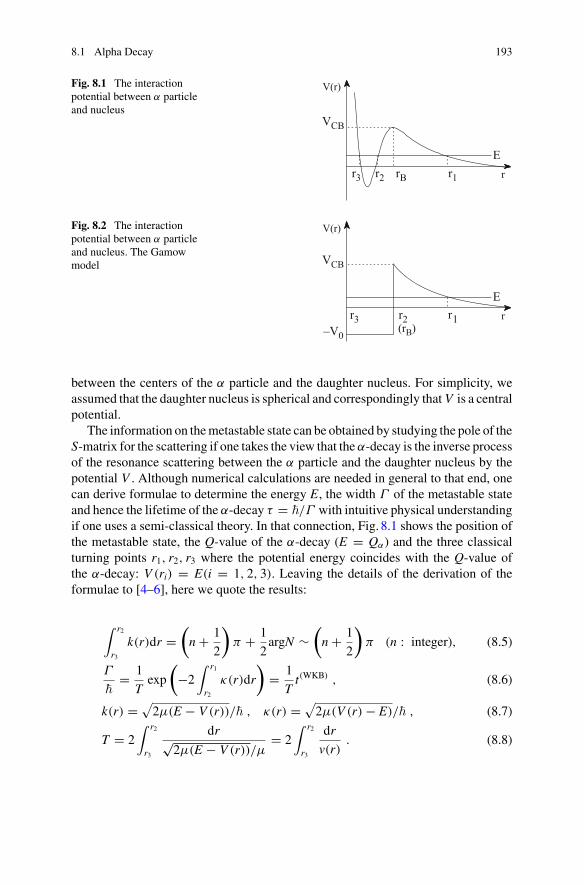
8.1 Alpha Decay 193
Fig. 8.1 The interactionpotential between α particleand nucleus
r
V(r)
ErB
VCB
r1r2r3
Fig. 8.2 The interactionpotential between α particleand nucleus. The Gamowmodel
r
V(r)
E
VCB
r1–V0
(rB)r2r3
between the centers of the α particle and the daughter nucleus. For simplicity, weassumed that the daughter nucleus is spherical and correspondingly that V is a centralpotential.
The information on themetastable state can be obtained by studying the pole of theS-matrix for the scattering if one takes the view that the α-decay is the inverse processof the resonance scattering between the α particle and the daughter nucleus by thepotential V . Although numerical calculations are needed in general to that end, onecan derive formulae to determine the energy E, the width Γ of the metastable stateand hence the lifetime of the α-decay τ = �/Γ with intuitive physical understandingif one uses a semi-classical theory. In that connection, Fig. 8.1 shows the position ofthe metastable state, the Q-value of the α-decay (E = Qα) and the three classicalturning points r1, r2, r3 where the potential energy coincides with the Q-value ofthe α-decay: V (ri) = E(i = 1, 2, 3). Leaving the details of the derivation of theformulae to [4–6], here we quote the results:
∫ r2
r3
k(r)dr =(
n + 1
2
)π + 1
2argN ∼
(n + 1
2
)π (n : integer), (8.5)
Γ
�= 1
Texp
(−2∫ r1
r2
κ(r)dr
)= 1
Tt(WKB) , (8.6)
k(r) = √2μ(E − V (r))/� , κ(r) = √
2μ(V (r) − E)/� , (8.7)
T = 2∫ r2
r3
dr√2μ(E − V (r))/μ
= 2∫ r2
r3
dr
v(r). (8.8)
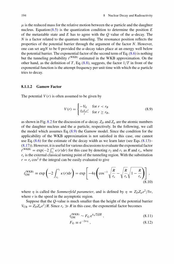
194 8 Nuclear Decay and Radioactivity
μ is the reduced mass for the relative motion between the α particle and the daughternucleus. Equation (8.5) is the quantization condition to determine the position Eof the metastable state and E has to agree with the Q value of the α-decay. TheN is a factor related to the quantum tunneling. The resonance position reflects theproperties of the potential barrier through the argument of the factor N . However,one can set argN to be 0 provided the α-decay takes place at an energy well belowthe potential barrier. The exponential factor of the second term of Eq. (8.6) is nothingbut the tunneling probability t(WKB) estimated in the WKB approximation. On theother hand, as the definition of T , Eq. (8.8), suggests, the factor 1/T in front of theexponential function is the attempt frequency per unit time with which the α particletries to decay.
8.1.1.2 Gamow Factor
The potential V (r) is often assumed to be given by
V (r) ={
−V0 for r < rBZDZαe2
r for r ≥ rB,(8.9)
as shown in Fig. 8.2 for the discussion of α-decay. ZD and Zα are the atomic numbersof the daughter nucleus and the α particle, respectively. In the following, we callthe model which assumes Eq. (8.9) the Gamow model. Since the condition for theapplicability of the WKB approximation is not satisfied in this case, one cannotuse Eq. (8.6) for the estimate of the decay width as we learn later (see Eqs. (8.13)–(8.17)). However, it is useful for various discussions to evaluate the exponential factort(WKB) = exp(−2
∫ r1r2
κ(r)dr) for this case by denoting r2 and r1 as R and re, wherere is the external classical turning point of the tunneling region. With the substitutionr = re cos2 θ the integral can be easily evaluated to give
t(WKB)GM ≡ exp
(−2∫ r1
r2
κ(r)dr
)= exp
[−4η
(cos−1
√R
re−√
R
re
√1 − R
re
)],
(8.10)
where η is called the Sommerfeld parameter, and is defined by η ≡ ZDZαe2/�v,where v is the speed in the asymptotic region.
Suppose that the Q-value is much smaller than the height of the potential barrierVCB = ZDZαe2/R. Since re � R in this case, the exponential factor becomes
t(WKB)GM ∼ FG e4
√2ηkR , (8.11)
FG ≡ e−2πη , (8.12)
8.1 Alpha Decay 195
where k is the wave number in the asymptotic region. The FG is called the Gamowfactor, and plays the principal role in governing the probability of quantum tunnelingwhen the decay energy is small. The contribution of the second factor e4
√2ηkR is much
smaller than that of the Gamow factor. However, it cannot be ignored or set equal to1 for the α-decay of heavy nuclei in order to keep the quantitative accuracy. In fact,it is larger than the pre-exponential factor which will be defined later.
8.1.1.3 Direct Method Based on the Gamow Model
In the case of the Gamow model, the wave functions are given by the sphericalBessel functions of the first kind in the potential region and by the Coulomb wavefunctions in the external region. Hence one can derive the formulae for the decaywidth by using them and the asymptotic form of the Coulomb wave function G0 [7].Leaving the derivation to AppendixA.8, here we quote the result for the case whenE � VCB. Letting T = 2R/v′, where v′ = �K/μ is the speed of the α particle insidethe potential well, i.e., at r < rB, we have
Γ
�= 1
Tt(D)GM , (8.13)
t(D)GM ∼ 4
k
K
1
G20(η, kR)
, (8.14)
1
G20(η, kR)
∼(2η
kR
)1/2
e−2πη e4√2ηkR ∼
(2η
kR
)1/2
t(WKB)GM , (8.15)
t(D)GM = 4
k
K
( re
R
)1/2t(WKB)GM = A(D)
GM t(WKB)GM , (8.16)
K ≡ √2μ(E + V0)/�, k = √
2μE/� . (8.17)
t(D)GM is the probability of the tunneling effect given by Eq. (A.127). Note that it differsfrom the value given by Eq. (8.11), which is obtained by simply applying the WKBapproximation, by the factor A(D)
GM.
8.1.1.4 Time-Dependent Perturbation Theory Based on the GamowModel: Two-Potential Approach
The two-potential approach [8] is also often used for the calculation of the α-decaywidth. In thismethod, one introduces the potential V1(r), which has an infinitely thickpotential barrier, i.e., V1(r) = −V0 for r < R and V1(r) = VCB for r ≥ R, and thepotential V2(r), which has only the Coulomb potential, i.e., V2(r) = VC(r) = ZDZαe2
r .The Gamow potential can be decomposed as
196 8 Nuclear Decay and Radioactivity
V (r) ={
V1(r) for r < R
V2(r) for r ≥ R ,(8.18)
by using these potentials. The α-decay width can be obtained by calculating thetransition probability from a bound state φn(r) with energy En in the potential V1(r)to a continuum state φE(r)with energy E close to En in the potential V2(r). Since theperturbation Hamiltonian is V (r) − V1(r), the transition probability per unit time isgiven by
Γ
�= 2π
�
∣∣∣∣∫
φ∗E(r)[V (r) − V1(r)]φn(r)dr
∣∣∣∣2
. (8.19)
One finally obtains3
Γ
�= �k1
μD2 exp
(−2∫ re
Rκ(r)dr
)= �k1
μD2e−2πηe4
√2ηkR ∼ �k1
μD2t(WKB)
GM ,
(8.20)
�k1μ
D2 = 2
R
(2
μ
)1/2
(VCB − E)1/2E + V0
VCB + V0, (8.21)
D ≡(2
R
)1/2 K√k21 + K2
; k1 = √2μ(VCB − E)/� . (8.22)
According to [8], the pre-exponential factor (�k1μ
)D2 represents the probability thatthe α particle appears at the nuclear surface per unit time.
8.1.1.5 Comparison of Three Methods
The formulae for the decay width in the three methods discussed in Sects. 8.1.1.1,8.1.1.3 and 8.1.1.4 contain the Gamow factor in common. However, the pre-exponential factor depends on the way of derivation of the formulae in each method.
The formulae introduced in Sect. 8.1.1.1 are superior in the sense that they canbe applied to smooth realistic potentials, since they have been derived based on theWKB approximation. However, one has to be careful when they are applied to theGamow model as they are, and when the tunneling probability t(WKB) in Eq. (8.6) isreplaced by the Gamow factor e−2πη or by the formula multiplied with the correctionfactor Eq. (8.11). Since the discussions in both Sect. 8.1.1.3 and 8.1.1.4 are based onthe Gamow model, their formulae must yield the correct result within the Gamowmodel, and should in principle give the same decay width.
As an example, let us consider the α-decay of 210Po. As we discuss in Sect.A.8,there exists an ambiguity for the potential describing the α-decay, and there are
3See [8] for the details of the derivation and physical interpretation. See also [9].
8.1 Alpha Decay 197
various potentials ranging from a shallow to a deep potentials.4 Here, we assumethat the wave function of the relative motion between the daughter nucleus and theα particle has 11 nodes by considering the Pauli exclusion principle. In this case, thepotential becomes a deep potential, and V0 = 108MeV, R = 7.92 fm as we show inSect.A.8. VCB is about 30MeV, while Q-value is 5.4MeV. Hence it holds that
V0 � VCB � Eα . (8.24)
In this case, the pre-exponential factor �k1μ
D2 in Eq. (8.20) approximately becomes1T 4
kα
K ( reR )1/2. The result of Sect. 8.1.1.3 given by Eqs. (8.13), (8.15), and (8.20) in
Sect. 8.1.1.4 thus become practically equivalent for the model which assumes a deeppotential for the potential between the daughter nucleus and the α particle.5
4Let us take a view of cluster model that a nucleus consists of two constituent clusters A and B. Inthe case of α-decay, the nucleus corresponds to the parent nucleus, and the clusters A and B to thedaughter nucleus and the emitted α particle, respectively. Accordingly, we first represent the totalwave function as the product of the intrinsic wave functions of the clusters A and B and the wavefunction for their relative motion. We then antisymmetrize with respect to the whole nucleons. Thisis called the resonating group method (RGM). If we represent the intrinsic wave functions of twoclusters in the harmonic oscillator model with the same oscillator parameter, then there exist ingeneral special states called either the Pauli forbidden states or the redundant states for the wavefunction of the relative motion because of the constraint that the total wave function has to beantisymmetric with respect to the exchange of any two nucleons. They are the states, for whichthe total wave function vanishes as the result of antisymmetrization. Consequently, there appearsambiguity in thewave functionof the relativemotion concerning the admixture of thePauli forbiddenstates, and it turns out that there exist several equivalent wave functions with different number ofnodes, which we denote by nr = 0, 1, . . . by excluding the node at the origin. Correspondingly,there appears an ambiguity for the potential describing the relative motion ranging from shallow todeep potentials. For example, if we represent 8Be as the product of two α particles and their relativemotion, then the 0s and 1s states are the Pauli forbidden states for the relative motion with angularmomentum 0. By counting the quantum number in the harmonic oscillator shell model, one canwrite the condition for the Pauli forbidden states as
2nr + � < N (SM)C − N (SM)
A − N (SM)B , (8.23)
when the angular momentum of the relativemotion is �. Here,N (SM)C ,N (SM)
A andN (SM)B are the total
quantum number of the whole nucleus (C) and of the constituent clusters (A) and (B) when theyare represented by the harmonic oscillator shell model. For example, in the case of α–α scatteringor in the case of the α-decay of 8Be, N (SM)
A = N (SM)B = 0, N (SM)
C = 4. Equation (8.23) is calledthe Wildermuth condition. In the case of the α-decay of 210Po, the right-hand side of Eq. (8.23) is(5 + 6) × 2, so that the states with nr = 11 and/or larger nr are the allowed states. Incidentally,the existence of the Pauli forbidden states is also the origin of the repulsive core in the potentialbetween complex nuclei. In the α–α scattering, the 0s and 1s states are the redundant states for� = 0 and the 0d state is the redundant state for � = 2. Hence there exists repulsive core in thepotential for these partial waves. On the other hand, there exists no redundant state for � = 4 andhigher partial waves, so that there is no repulsive core in the potential for those high partial waves.5Various methods to calculate the decay width have been numerically compared for the protondecay [10].
198 8 Nuclear Decay and Radioactivity
8.1.1.6 Preformation Factor—R-Matrix Theory
All the three methods so far discussed presume that the α particle with the samestructure as that of the α particle in nature exists inside the parent nucleus in advanceof the α-decay. Let us call such a point of view the potential model. On the otherhand, one can make a detailed description of the state of the parent nucleus using thewave functions of nucleons based on, e.g., the shell model or the cluster model. Insuch calculations the α particle is not presumed to exist in advance inside the nucleuswith the same structure as that in nature. For example, a simple shell model is basedon the thought that each nucleon inside a nucleus moves independently from eachother in the mean field except for the constraint due to the Pauli exclusion principle.In order to evaluate the α-decay width based on the study of nuclear structure by amany-body theory such as the shell model, it is necessary to estimate the formationprobability of α particle inside the nucleus prior to the decay. The formalism basedon the R-matrix theory6 is one of the representatives of such approaches which takesinto account the preformation probability, where the decay width is given by thefollowing formulae:
Γ = 2krcγ2L (rc)vL(rc) = 2PL(rc)γ
2L (rc) , (8.25)
vL(rc) ≡ 1
F2L(rc) + G2
L(rc)∼ 1
G2L(rc)
, (8.26)
γL(r) =(
�2
2μr
)1/2
YL(r) , (8.27)
YL(r)
r= 〈φαφDYLM(r)|ψP〉int,r . (8.28)
The FL and GL are the Coulomb wave functions. rc is chosen such that the effectof short-range force between the daughter nucleus and the emitted particle, i.e., theα particle in the case of alpha decay, is absent in the region r > rc, and is calledthe channel radius. vL(rc) is called the penetration factor, where the index L showsthat the decay takes place for the partial wave L.7,8 The ψP is the wave functionof the parent nucleus, and φD, φα are the intrinsic wave functions of the daughternucleus and the α particle, respectively. They are determined based on appropriate
6TheR-matrix theory is a theory to describe resonances in nuclear reactions. It describes the reactionby dividing the space into the internal region and the external region, i.e., the asymptotic regionwhere the nuclear force between the emitted nucleus and the remaining nucleus can be ignored. See[11–15].7As the asymptotic formula GL + iFL ∼ exp[i(ρ − η ln(2ρ) − Lπ/2+ σL)], where ρ = kr and σLbeing the Coulomb phase shift, indicates, the wave function which becomes the outgoing wave ofunit magnitude is given by ψL(r) = FL(r) + iGL(r) in the region r ≥ rc for the Gamow model.Hence the vL(rc) ≡ 1
F2L(rc)+G2
L(rc)gives the magnitude of the penetration probability from rc to the
outside of the potential barrier.8As it was shown by Eq. (8.14) in Sect. 8.1.1.3, v0 and the transmission coefficient t in the Gamowmodel are related as t(D)
GM ∼ 4 kK
1G20(krc)
∼ 4 kK v0(krc).
8.1 Alpha Decay 199
many-body theories such as the shell model, cluster model or mean-field theory. Thelower index int, r of Eq. (8.28) means to integrate over the intrinsic coordinates andthe angular coordinates of the relative motion. The YL(r)/r is therefore the radialwave function of the relative motion between the daughter nucleus and the α particle.γ 2
L (r) has the dimension of energy and called the reduced width. It gives a measure offormation probability of the α particle at the surface (r = rc) of the parent nucleus.It is often expressed as
γ 2L (rc) ≡ θ2(rc)γ
2W (rc) , γ 2
W (rc) = 3�2
2μr2c. (8.29)
γ 2W (rc) is the value of γ 2
L (rc) in the case when the initial state of the α-decay in theparent nucleus has such a structure that an α particle is clusterized and the radialwave function of the relative motion YL(r) = YL(r)/r distributes uniformly in theregion 0 ≤ r ≤ rc. It is called the Wigner limit [16].9 θ2 is the reduced width in unitsof the Wigner limit.
Exercise 8.1 Noting that G0(ρ = 0) = 1/C0(η) and C20(η) = 2πη(e2πη − 1)−1,
confirm that 1/G20 is proportional to the Gamow factor, which is the principal factor
to govern the tunneling probability, if η � 1.
Let us investigate the relation between the formulae for the α-decay widthdiscussed in Sect. 8.1.1.1, 8.1.1.3, and 8.1.1.4, and Eq. (8.25). If we denote themomentum for Y (r) in the region r < rc by pin, and estimate it as pinrc ∼ �
based on the uncertainty relation, we have
γ 2W
�= 3
2
�2
μ
1
rc
pin
�2∼ 3
T. (8.30)
Hence Eq. (8.25) can be expressed as
Γ
�= 1
Tt fP (8.31)
by writing the penetration probability as t, which is tentatively identified with PL(rc).fP ∝ θ2 represents the probability that the α particle exists inside the parent nucleusin advance of the decay. Let us therefore refer to it as the preformation factor.
The value of θ2 provides important information on the extent of clusterization inlight nuclei [18]. A large value of the reduced width for the α-decay corresponds to alarge preformation factor of the α particle, and suggests that the picture of the alphacluster structure holds. The preformation factor is ignored in some analyses of theα-decay. In that case, the effect of the preformation factor is effectively incorporatedin the parameters such as the depth V0 and the range parameter R of the potential.10
Reference [20] is an example of the calculation of θ2 based on the shell model.
9See [17] for the connection to the Teichmann–Wigner sum rule.10Here, we quote [19] as references for the analysis of α-decay.
200 8 Nuclear Decay and Radioactivity
Incidentally, for heavy particle decay such as the 14C emission, the possibility thatthe species of the emitted particle and its structure change on the way of decay dueto the channel coupling effects has also been discussed.
8.1.2 The Geiger–Nuttal Rule
The α-decay width strongly depends on the Q-value of the decay and the atomicnumber of the parent or daughter nuclei through the tunneling probability. Theirprincipal effects are expressed by the Gamow factor. Let us therefore express thedecay width, more precisely, the decay rate per unit time as
Γ
�= Ae−2πη (8.32)
by separating out the Gamow factor. Taking the logarithm of both sides and usingη ≡ ZDZαe2/�v, we obtain
log10Γ
�= log10 A − CZDE−1/2
α , (8.33)
C ≡ 2πe2
�c
√μc2
2Zα log10 e ≈ 1.72 . (8.34)
The factor A does not depend so much on the decaying system as long as weconsider nuclei in a region of similar mass number. Hence Eq. (8.33) suggests thatthe experimental data distribute almost along a straight line if we plot them by takinglog10 Γ/� as the ordinate and ZDE−1/2
α as the abscissa [12, 21]. This property iscalled the Geiger–Nuttal rule.
Incidentally, detailed information can be obtained from the analysis of the factorA, since it contains the information on the system such as the potential and thepreformation factor.
8.2 Fission
In Chap.2 we studied fission somewhat in detail with respect to nuclear instability.Here, we briefly discuss recent developments of the study of fission. As shownin Fig. 2.19 in a simplified fashion, fission is, in a general term, one of the decayprocesses of a metastable state, and occurs by quantum tunneling if the temperatureof the system is 0 or low, while occurs thermally, i.e., by thermal hopping, if thetemperature becomes sufficiently high. Figure8.3 schematically shows this situation.The critical temperature TC which divides the quantum decay and the thermal decayis given by
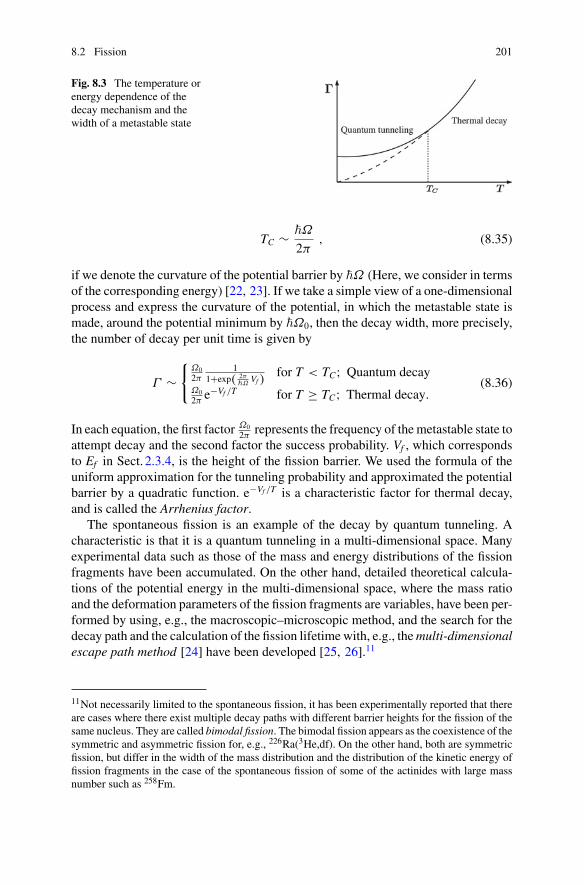
8.2 Fission 201
Fig. 8.3 The temperature orenergy dependence of thedecay mechanism and thewidth of a metastable state
TC ∼ �Ω
2π, (8.35)
if we denote the curvature of the potential barrier by �Ω (Here, we consider in termsof the corresponding energy) [22, 23]. If we take a simple view of a one-dimensionalprocess and express the curvature of the potential, in which the metastable state ismade, around the potential minimum by �Ω0, then the decay width, more precisely,the number of decay per unit time is given by
Γ ∼{
Ω02π
11+exp( 2π
�ΩVf )
for T < TC; Quantum decayΩ02π e
−Vf /T for T ≥ TC; Thermal decay.(8.36)
In each equation, the first factor Ω02π represents the frequency of themetastable state to
attempt decay and the second factor the success probability. Vf , which correspondsto Ef in Sect. 2.3.4, is the height of the fission barrier. We used the formula of theuniform approximation for the tunneling probability and approximated the potentialbarrier by a quadratic function. e−Vf /T is a characteristic factor for thermal decay,and is called the Arrhenius factor.
The spontaneous fission is an example of the decay by quantum tunneling. Acharacteristic is that it is a quantum tunneling in a multi-dimensional space. Manyexperimental data such as those of the mass and energy distributions of the fissionfragments have been accumulated. On the other hand, detailed theoretical calcula-tions of the potential energy in the multi-dimensional space, where the mass ratioand the deformation parameters of the fission fragments are variables, have been per-formed by using, e.g., the macroscopic–microscopic method, and the search for thedecay path and the calculation of the fission lifetimewith, e.g., themulti-dimensionalescape path method [24] have been developed [25, 26].11
11Not necessarily limited to the spontaneous fission, it has been experimentally reported that thereare cases where there exist multiple decay paths with different barrier heights for the fission of thesame nucleus. They are called bimodal fission. The bimodal fission appears as the coexistence of thesymmetric and asymmetric fission for, e.g., 226Ra(3He,df). On the other hand, both are symmetricfission, but differ in the width of the mass distribution and the distribution of the kinetic energy offission fragments in the case of the spontaneous fission of some of the actinides with large massnumber such as 258Fm.
202 8 Nuclear Decay and Radioactivity
The induced fission corresponds to the thermal decay if the excitation energy ishigh as it is the case for the fission induced by heavy-ion collisions. The formulafor the thermal decay given by the lower line of Eq. (8.36) is known as the formulaof the transition state theory by Bohr and Wheeler [27]. The Kramers formula [28]which takes into account the effect of friction,
Γ ∼{
γVf
T e−Vf /T when γ
2Ω < TVf
(the case of weak friction)Ω02π Ke−Vf /T when γ
2Ω > TVf
(the case of strong friction) ,(8.37)
where
K = 1
Ω
[√Ω2 + 1
4γ 2 − γ
2
](8.38)
is also often used as the basic formula for the decay width of the thermal fissionin calculating the competition between fission and the emission of particles such asneutrons by viewing the fission as a kind of Brownian motion [29, 30] in the externalfield and hence by formulating it in terms of the Fokker–Planck equation in the phasespace. γ is the friction or viscosity coefficient in the Fokker–Planck equation. K isthe factor which takes into account the effect of friction on the decay rate and iscalled the Kramers factor.12
The studies of the reaction mechanism of heavy-ion reactions and of variousphysical quantities governing the collision have significantly advanced since 1970s.In this procedure, various concepts have been introduced. They are, e.g., the completefusion reaction, where the colliding nuclei completely fuse and decay after a longtime, and the quasi-fission, which resembles the complete fusion concerning themass distribution of the reaction products, but differs in the angular distribution andthe deep inelastic collision (DIC), which is supposed to have a short reaction timebecause of the feature that the masses of the reaction products stay near the masses ofthe projectile and the target nuclei even though a large energy loss from the relativemotion is involved. Many experimental data have been accumulated in these studiesconcerning the mass and kinetic energy distributions of the reaction products suchas the fission fragments, and the number of emitted neutrons associated with fission.The theoretical approach which follows the time evolution of the system based onthe Langevin equation by simulating the reaction as a random walk (or stochasticprocess, or drunker’s walk or Wiener process) in a multi-dimensional space has beendeveloped as a powerful method to analyze these data by paying attention to thedissipation and associated fluctuation properties [35] (see also [36]).
12There appears in addition a multiplicative correction factor which takes into account the quantumfluctuation around the classical path if we relate the decay width to the imaginary part of theHelmholtz free energy [31] and evaluate the partition function by using the path integral method[32–34].
8.3 Electromagnetic Transitions 203
8.3 Electromagnetic Transitions
Anucleus in the ground state makes transitions to excited states by absorbing photon,while a nucleus in an excited state makes transition to the ground state or to lowerexcited states by emitting photon. One can extract much information on the structureof the nucleus such as the excitation energy, the spin and parity of each energylevel, the nuclear shape and the collectivity of each excitation motion through thesetransitions.
8.3.1 Multipole Transition, Reduced Transition Probability
The probability of the electromagnetic transition can be given to a good accuracy bythe Fermi golden rule in the first order perturbation theory,
Tfi = 2π
�|〈f |Hint|i〉|2g(Ef ) . (8.39)
Hint is the interaction between the nucleus and the electromagnetic field, and is givenby Eq. (A.173) as will be described in AppendixA.9. If we denote the initial and thefinal states of the nucleus by |ψi〉 and |ψf 〉, respectively, and express the state of theradiation field in the occupation number representation (see AppendixA.9.3), thenthe change of the state can be schematically written as
|i〉 = |ψi〉| · · · nλ · · · 〉 →{
|f 〉 = |ψf 〉| · · · nλ − 1 · · · 〉 for absorption,
|f 〉 = |ψf 〉| · · · nλ + 1 · · · 〉 for emission.(8.40)
Also, it holds that �kc = |Ef − Ei| because of the energy conservation if we denotethe wave length of the photon by λ = 2π/k, and the energy of the initial and finalstates of the nucleus by Ei and Ef , respectively.
g(Ef ) is the number of final states of the radiation field per unit energy. If weconsider the magnetic radiation as an example, we have
0 = jI(knR) ∼ 1
knRsin(
knR − π
2I)
(8.41)
from the boundary condition given by Eq. (A.167). Here, we considered R → ∞.Hence it follows that
knR = π
2I + nπ, n = 0,±1,±2, · · · . (8.42)
204 8 Nuclear Decay and Radioactivity
The density of the final state of the radiation field g is thus given by
g(k) = 1
ΔE(k)= 1
�(Δk)c= 1
�πR c
= R
�cπ. (8.43)
Using the explicit expressions of the vector fields, Eqs. (A.164) and (A.165), theexpression of the normalization constant Eq. (A.169), and the formula for the leveldensity Eq. (8.43), we can write the transition probability per unit time by emittingone photon of the (λ, k, I, M) type as
Tfi(E, kIM) = 8πk
�
∣∣∣∣⟨f
∣∣∣∣ 1ck
∫j · ∇ × jI(kr)YIIMdr
∣∣∣∣ i⟩∣∣∣∣
2
, (8.44)
Tfi(M, kIM) = 8πk
�
∣∣∣∣⟨f
∣∣∣∣1c∫
j · jI(kr)YIIMdr
∣∣∣∣ i⟩∣∣∣∣
2
. (8.45)
Let us write the Tfi, in general, as
Tfi(λ, kIM) = 8π(I + 1)
�I[(2I + 1)!!]2(
Eγ
�c
)2I+1 ∣∣∣〈f |M (λ, kIM)|i〉∣∣∣2 (8.46)
by using the multipole transition operator M (λ, kIM).In nuclear physics, the long wave length approximation usually well applies.
Namely, it well holds thatkR � 1 (8.47)
if we denote the nuclear radius by R. Equation (8.47) is equivalent to13
Eγ = �kc � �c
R= �c
r0A−1/3 ≈ 197A−1/3 MeV . (8.48)
In the long wave length approximation, using
jI(kr) ∼ (kr)I
(2I + 1)!![1 − 1
2
(kr)2
2I + 3+ · · ·
], (8.49)
we can show that the multipole transition operators are nothing but the electricmultipole and the magnetic multipole operators introduced in Sect. 4.2 as
M (E, kIM) ≈∫
ρrI YIMdr = QIM , (8.50)
M (M, kIM) ≈ 1
c(I + 1)
∫(r × j) · ∇(rIYIM)dr = MIM . (8.51)
13Particle decay usually occurs with a higher probability when a high energy γ ray is emitted.
8.3 Electromagnetic Transitions 205
Exercise 8.2 Show that the wave length of photons of 1MeV is about 400π fm.
One usually does not distinguish the difference of the orientation of the angularmomentum of the nucleus except for the experiments related to polarization. Bytaking average with respect to the initial value Mi of the z component of the angularmomentum of the nucleus, and sum over the value Mf in the final state, the totalelectric or magnetic transition probability with multipolarity I is given by
Tfi(λ, I) = 1
2Ii + 1
∑Mi,Mf ,M
Tfi(λ, kIM) , (8.52)
where Ii is the angular momentum of the initial state of the nucleus. Performing thesum in Eq. (8.52) by using the Wigner–Eckart theorem and the properties of the 3jsymbol or the Clebsch–Gordan coefficients, we obtain
Tfi(λ, I) = 8π(I + 1)
�I[(2I + 1)!!]2(
Eγ
�c
)2I+1
B(λI; Ii → If ) . (8.53)
Here, B(λ) is called the reduced transition probability, and is given by
B(EI; Ii → If ) = 1
2Ii + 1|〈f ‖QI‖i〉|2 (8.54)
and
B(MI; Ii → If ) = 1
2Ii + 1|〈f ‖MI‖i〉|2 (8.55)
for the electric and magnetic transitions, respectively.
8.3.2 General Consideration of the Selection Rule and theMagnitude
If one denotes the angular momentum and parity of the initial and final states byIi,Πi and If ,Πf , then the selection rules,
|Ii − If | ≤ I ≤ Ii + If , ΠiΠλIΠf = 1 , (8.56)
hold due to the structure of the transitionmatrices 〈If Mf |QIM |IiMi〉, 〈If Mf |MIM |IiMi〉.ΠλI is the parity of the multipole radiation, and is given by
ΠEI = (−1)I , ΠMI = (−1)I+1 , (8.57)
because the interaction with the radiation field is given by Hint ∝ A · j.
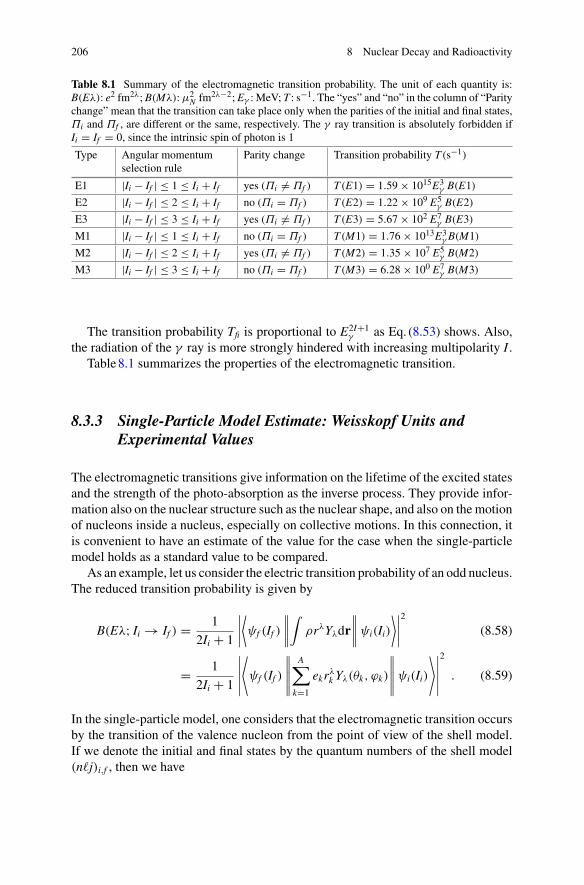
206 8 Nuclear Decay and Radioactivity
Table 8.1 Summary of the electromagnetic transition probability. The unit of each quantity is:B(Eλ): e2 fm2λ; B(Mλ):μ2
N fm2λ−2; Eγ : MeV; T : s−1. The “yes” and “no” in the column of “Paritychange” mean that the transition can take place only when the parities of the initial and final states,Πi and Πf , are different or the same, respectively. The γ ray transition is absolutely forbidden ifIi = If = 0, since the intrinsic spin of photon is 1
Type Angular momentumselection rule
Parity change Transition probability T(s−1)
E1 |Ii − If | ≤ 1 ≤ Ii + If yes (Πi �= Πf ) T(E1) = 1.59 × 10¹⁵E3γ B(E1)
E2 |Ii − If | ≤ 2 ≤ Ii + If no (Πi = Πf ) T(E2) = 1.22 × 10⁹ E5γ B(E2)
E3 |Ii − If | ≤ 3 ≤ Ii + If yes (Πi �= Πf ) T(E3) = 5.67 × 10² E7γ B(E3)
M1 |Ii − If | ≤ 1 ≤ Ii + If no (Πi = Πf ) T(M1) = 1.76 × 10¹³E3γ B(M1)
M2 |Ii − If | ≤ 2 ≤ Ii + If yes (Πi �= Πf ) T(M2) = 1.35 × 10⁷ E5γ B(M2)
M3 |Ii − If | ≤ 3 ≤ Ii + If no (Πi = Πf ) T(M3) = 6.28 × 100 E7γ B(M3)
The transition probability Tfi is proportional to E2I+1γ as Eq. (8.53) shows. Also,
the radiation of the γ ray is more strongly hindered with increasing multipolarity I .Table8.1 summarizes the properties of the electromagnetic transition.
8.3.3 Single-Particle Model Estimate: Weisskopf Units andExperimental Values
The electromagnetic transitions give information on the lifetime of the excited statesand the strength of the photo-absorption as the inverse process. They provide infor-mation also on the nuclear structure such as the nuclear shape, and also on the motionof nucleons inside a nucleus, especially on collective motions. In this connection, itis convenient to have an estimate of the value for the case when the single-particlemodel holds as a standard value to be compared.
As an example, let us consider the electric transition probability of an odd nucleus.The reduced transition probability is given by
B(Eλ; Ii → If ) = 1
2Ii + 1
∣∣∣∣⟨ψf (If )
∥∥∥∥∫
ρrλYλdr
∥∥∥∥ψi(Ii)
⟩∣∣∣∣2
(8.58)
= 1
2Ii + 1
∣∣∣∣∣⟨ψf (If )
∥∥∥∥∥A∑
k=1
ekrλk Yλ(θk, ϕk)
∥∥∥∥∥ψi(Ii)
⟩∣∣∣∣∣2
. (8.59)
In the single-particle model, one considers that the electromagnetic transition occursby the transition of the valence nucleon from the point of view of the shell model.If we denote the initial and final states by the quantum numbers of the shell model(n�j)i,f , then we have
8.3 Electromagnetic Transitions 207
Bsp(Eλ; Ii → If ) = 1
2Ii + 1
∣∣〈(n�j)f ‖eeffrλYλ‖(n�j)i〉
∣∣2 , (8.60)
which becomes
Bsp(Eλ; Ii → If ) = e2eff2λ + 1
4π
∣∣∣∣⟨jiλ
1
20
∣∣∣∣jf 12⟩∣∣∣∣
2
× ∣∣〈(n�j)f |rλ|(n�j)i〉∣∣2 1 + (−1)�i+�f +λ
2(8.61)
after some calculations. The eeff , named the effective charge, effectively takes intoaccount the effect of the nucleons other than the valence nucleon due to, e.g., thecore polarization. Let us consider especially the case when ji = I + 1/2, jf = 1/2,and approximate the Clebsch–Gordan coefficient by the asymptotic value:
⟨jiλ
1
20
∣∣∣∣jf 12⟩
= (−1)I 1√2I + 1
√2(I + 1)
2I + 1∼ (−1)I 1√
2I + 1, (8.62)
and furthermore estimate 〈f |rI |i〉 as
〈f |rI |i〉 =∫ ∞
0Rf (r)r
IRi(r)r2dr =
∫ R0
0 rI r2dr∫ R0
0 r2dr= 3
I + 3RI0 , (8.63)
where Rf (r) and Ri(r) are the radial wave functions of the final and initial states, byassuming that the nucleon uniformly distributes inside the region of radius R0. Wethen obtain
BW (EI) = e21
4π
(3
I + 3
)2
R2I0 . (8.64)
We have set eeff to the elementary charge e in order to have a measure of the single-particle transition. By introducing similar approximations, and further approximatingI2(gs − 2(I + 1)−1g�)
2 ≈ 10 [37], we obtain
BW (MI) = 10
π
(3
I + 3
)2
R2I−20 μ2
N (8.65)
for the magnetic transition [37]. The values given by Eqs. (8.64) and (8.65) are calledtheWeisskopf unit and play an important role in judging the properties of the nucleus,especially concerning whether a certain motion of the nucleus is of single-particlenature or of a collective nature.
For even–even nuclei as well, by taking the initial and final states to be
|0+g.s.〉 = |(n�j)2π ; 0+〉, |2+
1 〉 = |(n�j)2π ; 2+1 〉 , (8.66)
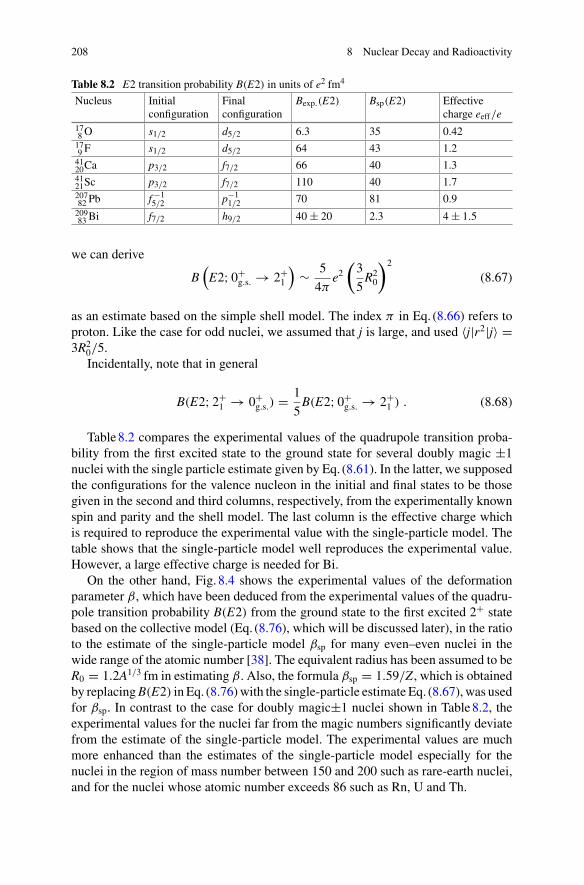
208 8 Nuclear Decay and Radioactivity
Table 8.2 E2 transition probability B(E2) in units of e2 fm4
Nucleus Initialconfiguration
Finalconfiguration
Bexp.(E2) Bsp(E2) Effectivecharge eeff/e
178 O s1/2 d5/2 6.3 35 0.42179 F s1/2 d5/2 64 43 1.24120Ca p3/2 f7/2 66 40 1.34121Sc p3/2 f7/2 110 40 1.720782 Pb f −1
5/2 p−11/2 70 81 0.9
20983 Bi f7/2 h9/2 40 ± 20 2.3 4 ± 1.5
we can derive
B(
E2; 0+g.s. → 2+
1
)∼ 5
4πe2(3
5R20
)2
(8.67)
as an estimate based on the simple shell model. The index π in Eq. (8.66) refers toproton. Like the case for odd nuclei, we assumed that j is large, and used 〈j|r2|j〉 =3R2
0/5.Incidentally, note that in general
B(E2; 2+1 → 0+
g.s.) = 1
5B(E2; 0+
g.s. → 2+1 ) . (8.68)
Table8.2 compares the experimental values of the quadrupole transition proba-bility from the first excited state to the ground state for several doubly magic ±1nuclei with the single particle estimate given by Eq. (8.61). In the latter, we supposedthe configurations for the valence nucleon in the initial and final states to be thosegiven in the second and third columns, respectively, from the experimentally knownspin and parity and the shell model. The last column is the effective charge whichis required to reproduce the experimental value with the single-particle model. Thetable shows that the single-particle model well reproduces the experimental value.However, a large effective charge is needed for Bi.
On the other hand, Fig. 8.4 shows the experimental values of the deformationparameter β, which have been deduced from the experimental values of the quadru-pole transition probability B(E2) from the ground state to the first excited 2+ statebased on the collective model (Eq. (8.76), which will be discussed later), in the ratioto the estimate of the single-particle model βsp for many even–even nuclei in thewide range of the atomic number [38]. The equivalent radius has been assumed to beR0 = 1.2A1/3 fm in estimating β. Also, the formula βsp = 1.59/Z , which is obtainedby replacingB(E2) in Eq. (8.76)with the single-particle estimate Eq. (8.67), was usedfor βsp. In contrast to the case for doubly magic±1 nuclei shown in Table8.2, theexperimental values for the nuclei far from the magic numbers significantly deviatefrom the estimate of the single-particle model. The experimental values are muchmore enhanced than the estimates of the single-particle model especially for thenuclei in the region of mass number between 150 and 200 such as rare-earth nuclei,and for the nuclei whose atomic number exceeds 86 such as Rn, U and Th.
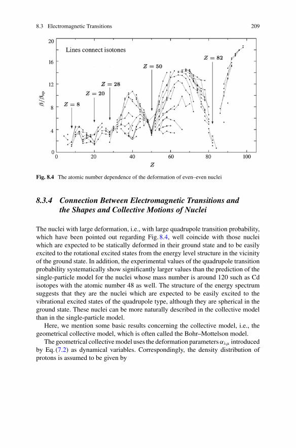
8.3 Electromagnetic Transitions 209
Fig. 8.4 The atomic number dependence of the deformation of even–even nuclei
8.3.4 Connection Between Electromagnetic Transitions andthe Shapes and Collective Motions of Nuclei
The nuclei with large deformation, i.e., with large quadrupole transition probability,which have been pointed out regarding Fig. 8.4, well coincide with those nucleiwhich are expected to be statically deformed in their ground state and to be easilyexcited to the rotational excited states from the energy level structure in the vicinityof the ground state. In addition, the experimental values of the quadrupole transitionprobability systematically show significantly larger values than the prediction of thesingle-particle model for the nuclei whose mass number is around 120 such as Cdisotopes with the atomic number 48 as well. The structure of the energy spectrumsuggests that they are the nuclei which are expected to be easily excited to thevibrational excited states of the quadrupole type, although they are spherical in theground state. These nuclei can be more naturally described in the collective modelthan in the single-particle model.
Here, we mention some basic results concerning the collective model, i.e., thegeometrical collective model, which is often called the Bohr–Mottelson model.
The geometrical collectivemodel uses the deformation parametersαλμ introducedby Eq. (7.2) as dynamical variables. Correspondingly, the density distribution ofprotons is assumed to be given by
210 8 Nuclear Decay and Radioactivity
ρp(r) = ρ(0)p Θ[R(θ, ϕ) − r]
= ρ(0)p Θ
⎡⎣R0
⎛⎝1 + α00 +
∞∑λ=2
λ∑μ=−λ
α∗λμYλμ(θ, ϕ)
⎞⎠− r
⎤⎦ (8.69)
using the step function Θ(x).14 The operator of the electric transition is then givenby
Qλμ = e∫
Vρp(r)rλYλμ(θ, ϕ)d3r ∼ eZ
3
4πRλ0 αλμ . (8.70)
Here, we truncated the sum by the first order of the operator of the deformationparameter.15
For spherical nuclei, if we approximate the surface vibration by the harmonicoscillator model, then the quadrupole transition probability from the first excitedstate to the ground state is given by
B(E2; 2+1 → 0+
g.s.) =(
eZ3
4πR20
)2�
2B2Ω2, (8.71)
if the first excited state is the one phonon state with the angular momentum and parity2+. The �Ω2 and B2 represent the excitation energy and the mass parameter of thequadrupole vibration, respectively.16
Exercise 8.3 Derive the expressions ofB(E2) from the twophonon states 0+2 , 2+
2 , 4+1
of the quadrupole vibration to the one phonon state 2+1 and discuss their ratios to
B(E2; 2+1 → 0+
g.s.).
On the other hand, for axially symmetric even–even nuclei with quadrupole defor-mation, the Euler anglesω = {φ, θ, ψ}which specify the directions of principal axesbecome the variables for the rotational motion and the total wave function is givenby
|ΨIMK〉 =(
2I + 1
16π2(1 + δK0)
)1/2 [D I
MK(ω)ΦK(q) + (−1)I+KD IM−KΦK(q)
],
(8.72)whereD I
MK is theWignerD function, andK is the component of the angular momen-tum along the direction of the symmetry axis. ΦK(q) is the wave function of theintrinsic motions, and ΦK(q) is the wave function which is obtained by rotating
14Θ(x) = 1 (x ≥ 0), Θ(x) = 0 (x < 0).15See p.13 of [39] for the expression including higher order terms.16The values of �Ω2 and B2 can be theoretically estimated in the liquid-drop model which viewsthe nucleus as an irrotational incompressible fluid. However, the resulting values are quantitativelyin significant disagreement with the experimental data. Instead, more reliable estimates can beobtained phenomenologically from the experimental values of the excitation energy of the firstexcited 2+ state E2 and of B(E2; 2+
1 → 0+g.s.).
8.3 Electromagnetic Transitions 211
ΦK(q) by 180◦ around the second axis when the symmetry axis is taken to be thethird axis. The operator of the electric quadrupole moment and the E2 transition isgiven by
Qλμ ∼(
5
16π
)1/2
eQ0Dλμ0 , (8.73)
Q0 =(16π
5
)1/2
Z3
4πR20β , (8.74)
where λ = 2. Q0 is the intrinsic quadrupole moment.Using Eqs. (8.72)–(8.74) and the properties of the D function, one can show
that the electric quadrupole transition probability within a rotational band with thequantum number K is given by
B(E2; KI1 → KI2) = 5
16πe2Q2
0〈I12K0|I2K〉2 . (8.75)
Especially, the value of B(E2) from the first excited 2+1 state to the ground state 0+
g.s.of the ground state rotational band with K = 0 of even–even nuclei is given by
B(E2; 2+1 → 0+
g.s.) = 1
5
(3
4πZeR2
0
)2
β2 . (8.76)
Equation (8.76) shows that the magnitude of B(E2) increases proportionally to thesquare of the deformation β.17,18 Note that the electromagnetic transition probabili-
17One can estimate the deformation parameter β, more precisely βR20, from the experimental data of
B(E2) by using Eq. (8.76). However, B(E2) gives only the magnitude of the deformation parameter.One of the standard methods to determine the sign is to use the so-called reorientation effectin the Coulomb excitation. Recently, it has been attempted to precisely determine the deformationincluding the sign through the analyses of heavy-ion fusion reactions at energies below the Coulombbarrier [40–45].18The transition from high excited states to lower states within a nucleus can take place not onlyby the electromagnetic transition which emits a photon, but by ejecting an electron with the energyreleased in the decay. The latter process is called the internal conversion (see [46] for details).Hence the total transition probability is given by
w = wγ + we = (1 + α)wγ , (8.77)
α ≡ we/wγ , (8.78)
if we denote the transition probability by emitting photon by wγ , and the transition probabilityby the internal conversion process by we. α is called the internal conversion coefficient. If thetransition energy is large to some extent, then α is small, so that one can ignore the contribution ofthe internal conversion. On the other hand, the internal conversion becomes the main decay processif the excitation energy of the first excited 2+
1 state is small as in the case of 23892 U, where it is about45keV. Equation (8.76) holds in this case as well. However, care should be taken when one tries toestimate the magnitude of β from the lifetime of the 2+
1 state.
212 8 Nuclear Decay and Radioactivity
ties between different states within a rotational band are related to each other throughthe Clebsch–Gordan coefficients as is given by Eq. (8.75) in the case of ideal rota-tional motion, where the deformation does not change with the angular momentum,namely, where the intrinsic state does not change in the ground and excited states.19
References
1. H.J. Rose, G.A. Jones, Nature 307, 245 (1984)2. B. Blank, M.J.G. Borge, Prog. Part. Nucl. Phys. 60, 403 (2008); B. Blank, M. Płoszajczak.
Rep. Prog. Phys. 71, 046301 (2008)3. K. Kato, K. Ikeda, Butsuri 61, 814 (2006); T. Myo, Y. Kikuchi, H. Masui, K. Kato. Prog. Part.
Nucl. Phys. 79, 1 (2014)4. D.M. Brink, N. Takigawa, Nucl. Phys. A 279, 159 (1977)5. S.Y. Lee, N. Takigawa, Nucl. Phys. A 308, 189 (1978)6. S.Y. Lee, N. Takigawa, C. Marty, Nucl. Phys. A 308, 161 (1978)7. M. Abramowitz, I.A. Stegun, Handbook of Mathematical Functions with Formulas, Graphs,
and Mathematical Tables (Dover, London, 1978)8. M. Nogami, Nuclear Physics (Shoukabou, Tokyo, 1973). Japanese edn.9. D.F. Jackson, M. Rhoades-Brown, Ann. Phys. (NY) 105, 151 (1977); S. A. Gurvitz, G. Kalber-
mann, Phys. Rev. Lett. 59, 262 (1987); S. A. Gurvitz. Phys. Rev. A 38, 1747 (1988)10. S. Åberg, P.B. Semmes, W. Nazarewicz, Phys. Rev. C 56, 1762 (1997)11. J.M. Blatt, V.F. Weiskopf, Theoretical Nuclear Physics (Wiley, New York, 1952)12. M.A. Preston, Physics of the Nucleus (Addison-Wesley, London, 1962)13. K. Kikuchi, M. Kawai, Nuclear Matter and Nuclear Reactions (North-Holland, Amsterdam,
1968)14. S. Yoshida, M. Kawai, Nuclear Reactions (Asakura, Tokyo, 2002). Japanese edn.15. A.M. Lane, R.G. Thomas, Rev. Mod. Phys. 30, 257 (1958)16. E.P. Wigner, Phys. Rev. 70, 606 (1946); E.P. Wigner, L. Eisenbud. Phys. Rev. 72, 29 (1947)17. T. Teichman, E.P. Wigner, Phys. Rev. 87, 123 (1952)
19Here, we add comments on the liquid-drop model. The experimental data show systematics givenby
E2+1
B(E2; 2+1 → 0+
g.s.) ≈ (25 ± 8)Z2
A
[MeV e2 fm4
]∝ Z2/A . (8.79)
On the other hand, the liquid-drop model leads to
�Ω2B(E2) ∝ Z2R40/B2 ∝ Z2R4
0/AR20 ∝ Z2A2/3/A ∼ Z2A−1/3 (8.80)
for vibrational excitations.The prediction of the liquid-dropmodel Eq. (8.80) has a different mass number dependence from
that of the experimental data given by Eq. (8.79). One reason of the discrepancy is the quantummechanical effect, which plays important roles in nuclear physics. It is necessary to treat nucleus asa quantum liquid in order to handle nucleus in the liquid-drop model in a quantitatively proper way.For example, the classical liquid-drop model evaluates the potential energy by taking into accountthe effect of deformation only in the ordinary space in deriving the Hamiltonian for collectivemotions. Accurately, however, one needs to consider the effects of deformation in the momentumspace as well as suggested by the uncertainty principle in quantum mechanics. This effect showsup, for example, in the vibrational excited states such as the giant quadrupole resonance (GQR)[39]. The discrepancy between the experimental data and the prediction of the liquid-drop modelappears also regarding the moment of inertia of deformed nuclei.
References 213
18. A. Arima, H. Horiuchi, K. Kubodera, N. Takigawa, Adv. Nucl. Phys. 5, 345 (1972)19. B. Buck, A.C. Merchant, S.M. Perez, Phys. Rev. C 45, 2247 (1992); B. Buck, J. C. Johnson,
A. C. Merchant, S. M. Perez. Phys. Rev. C 53, 2841 (1996)20. I. Tonozuka, A. Arima, Nucl. Phys. A 323, 45 (1979)21. C.M. Lederer, V. Shirley, Table of Isotopes, 7th edn. (Wiley, New York, 1978)22. P. Hänggi, P. Talkner, M. Borkovec, Rev. Mod. Phys. 62, 251 (1990). and references therein23. U. Weiss, Quantum Dissipative Systems (World Scientific, Singapore, 1999)24. P. L. Kapur, R. Peierls, Proc. Roy. Soc. London A 163, 606 (1937); A. Schmid, Ann. Phys.
(NY) 170, 333 (1986)25. T. Kindo, A. Iwamoto, Phys. Lett. B 225, 203 (1989)26. N. Takigawa, K. Hagino, M. Abe, Phys. Rev. C 51, 187 (1995)27. N. Bohr, J.A. Wheeler, Phys. Rev. 56, 426 (1939)28. H.A. Kramers, Physica 7(284), 284 (1940)29. R.Kubo,M.Toda,N.Hashitsume, Statistical Physics II, Non-equilibrium Statistical Mechanics
(Springer, New York, 1985)30. H. Risken, The Fokker-Planck Equation (Springer, Berlin, 1989)31. J.S. Langer, Ann. Phys. (NY) 41, 374 (1967); I. K. Affleck. Phys. Rev. Lett. 46, 388 (1981)32. R.P. Feynman, A.R. Hibbs, Quantum Mechanics and Path Integrals (McGraw-Hill, New York,
1965)33. H. Grabert, P. Olschowski, U. Weiss, Phys. Rev. B 36, 1931 (1987)34. N. Takigawa, M. Abe, Phys. Rev. C 41, 2451 (1990)35. Y. Abe, C. Gregoire, H. Delagrange, J. Phys. 47, C4 (1986); T. Wada, Y. Abe, N. Carjan, Phys.
Rev. Lett. 70, 3538 (1993); Y. Abe, S. Ayik, P.-G. Reinhard, E. Suraud, Phys. Rep. 275, 49(1996)
36. P. Fröbrich, R. Lipperheide, Theory of Nuclear Reactions (Clarendon Press, Oxford, 1996)37. Aage Bohr, Ben R. Mottelson, Nuclear Structure, vol. I (Benjamin, New York, 1969)38. S. Raman, C.W. Nestor Jr., P. Tikkanen, At. Data Nucl. Data Tables 78(1), 1 (2001)39. P. Ring, P. Schuck, The Nuclear Many-Body problem (Springer, Berlin, 1980)40. A.B. Balantekin, N. Takigawa, Rev. Mod. Phys. 70, 77 (1998)41. M. Dasgupta, D.J. Hinde, N. Rowley, A.M. Stefanini, Ann. Rev. Nucl. Part. Sci. 48, 401 (1998)42. K. Hagino, N. Rowley, A.T. Kruppa, Comp. Phys. Commun. 123, 143 (1999)43. H. Esbensen, Nucl. Phys. A 352, 147 (1981)44. K. Hagino, N. Takigawa, Butsuri 57, 588 (2002)45. K. Hagino, N. Takigawa, Prog. Theor. Phys. 128, 1001 (2012)46. K. Yagi, Nuclear Physics (Asakura, Tokyo, 1971). Japanese edn.
Chapter 9Synthesis of Elements
Abstract It is a long-standing intriguing problem to explore the synthesis ofelements, and extensive studies are going on (See Clayton (Principles of StellarEvolution and Nucleosynthesis, The University of Chicago Press, Chicago, 1968,[1]), Rolfs and Rodney (Cauldrons in the Cosmos, The University of Chicago Press,Chicago, 1988, [2]), Thompson and Nunes (Nuclear Reactions for Astrophysics:Principles, Calculation and Applications of Low-Energy Reactions, Cambridge Uni-versity Press, Cambridge, 2009, [3]), VHS Element Genesis—Solving the Mystery,2001, [4]). Roughly speaking, the synthesis of elements can be divided into the pri-mordial nucleosynthesis, which is also called the Big Bang nucleosynthesis, and thestellar nucleosynthesis. The light elements such as deuterons, He and Li have beensynthesized by nuclear reactions within 3–15min after the Big Bang. This is the BigBang nucleosynthesis. It terminates at the elements of mass number 7, since thereis no stable nucleus of mass number 8. Stars started to be formed about one billionyears later. Then, thermal nuclear reactions took place inside stars, and nuclei up toFe, which has the largest binding energy per nucleon, have been successively syn-thesized depending on the mass of each star. (Precisely speaking, the nucleus whichhas the largest binding energy per nucleon is 62
28Ni as remarked in Chap.2.) Nucleibeyond Fe are synthesized either slowly by the neutron capture reactions called slowprocess (s-process) inside red giant stars, or synthesized by the explosive astrophys-ical phenomenon called rapid process (r-process). Nuclei with extremely large massnumber such as U are thought to be synthesized at the supernovae explosion, whichis one of the last stages of stars. In this chapter we learn some basics concerning thenuclear reactions related to nucleosynthesis (See Clayton (Principles of Stellar Evo-lution and Nucleosynthesis, 1968, [1]), Rolfs and Rodney (Cauldrons in the Cosmos,1988, [2]), Thompson and Nunes (Nuclear Reactions for Astrophysics: Principles,Calculation and Applications of Low-Energy Reactions, Cambridge UniversityPress, Cambridge, 2009, [3]) for details).
9.1 The Astrophysical S-Factor and Gamow Factor
The nuclear reactions between two charged particles in stars occur with the collisionenergy much lower than the Coulomb barrier like the proton–proton reactions in the
© Springer Japan 2017N. Takigawa and K. Washiyama, Fundamentals of Nuclear Physics,DOI 10.1007/978-4-431-55378-6_9
215
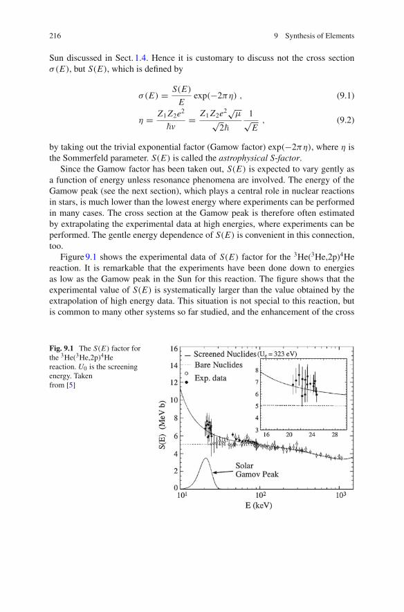
216 9 Synthesis of Elements
Sun discussed in Sect. 1.4. Hence it is customary to discuss not the cross sectionσ(E), but S(E), which is defined by
σ(E) = S(E)
Eexp(−2πη) , (9.1)
η = Z1Z2e2
�v= Z1Z2e2
√μ√
2�
1√E
, (9.2)
by taking out the trivial exponential factor (Gamow factor) exp(−2πη), where η isthe Sommerfeld parameter. S(E) is called the astrophysical S-factor.
Since the Gamow factor has been taken out, S(E) is expected to vary gently asa function of energy unless resonance phenomena are involved. The energy of theGamow peak (see the next section), which plays a central role in nuclear reactionsin stars, is much lower than the lowest energy where experiments can be performedin many cases. The cross section at the Gamow peak is therefore often estimatedby extrapolating the experimental data at high energies, where experiments can beperformed. The gentle energy dependence of S(E) is convenient in this connection,too.
Figure9.1 shows the experimental data of S(E) factor for the 3He(3He,2p)4Hereaction. It is remarkable that the experiments have been done down to energiesas low as the Gamow peak in the Sun for this reaction. The figure shows that theexperimental value of S(E) is systematically larger than the value obtained by theextrapolation of high energy data. This situation is not special to this reaction, butis common to many other systems so far studied, and the enhancement of the cross
Fig. 9.1 The S(E) factor forthe 3He(3He,2p)4Hereaction. U0 is the screeningenergy. Takenfrom [5]
9.1 The Astrophysical S-Factor and Gamow Factor 217
section has been attempted to be explained in terms of the screening effect due to,e.g., the electrons of the target nucleus.
9.2 Gamow Peak
If we denote the reaction rate per pair of colliding nuclei by λ,1 then it is given by
λ = 〈σv〉 =∫
σ(E)v(E)φ(v)dv . (9.3)
Here, φ(v) is the normalized Maxwell–Boltzmann distribution, and is given by
φ(v)dv = 2√π
β3/2 exp(−βE)√EdE , (9.4)
with β = 1/kT , where T and k are the temperature of the star and the Boltzmannconstant, respectively.
Inserting Eqs. (9.1) and (9.4) into Eq. (9.3), and using the definition of theSommerfeld parameter Eq. (9.2), we obtain
λ =√
8
μπβ3/2
∫ ∞
0S(E) exp
(−βE − bE−1/2)dE , (9.5)
b = π Z1Z2e2√2μ
�. (9.6)
b2 is called the Gamow energy.The exponential factor in the integrand of Eq. (9.5) is sharply peaked at an energy
because of the competition between the Gamow factor and the Maxwell distribution.Since S(E) is a gentle function of energy unless resonances are involved, one canapply the method of steepest descent to calculate the integral with little error. Fromthe condition
d
dE
(βE + bE−1/2) = 0 , (9.7)
the saddle point energy can be obtained as
E0 =(
b
2β
)2/3
. (9.8)
E0 is called the Gamow peak. Finally, the reaction rate is given by
λ ≈ 4√2√3
1√μE1/20 βS0e
−3βE0 , (9.9)
where S0 = S(E0).
1The actual reaction rate per pair is given by multiplying the pair density.
218 9 Synthesis of Elements
Exercise 9.1 Prove Eq. (9.9) based on the formula of the method of steepest descent
∫g(x)e− f (x)dx ≈
√2π
f ′′(x0)g(x0)e
− f (x0),
where x0 and f ′′ are the position of the saddle point and the second derivative of f ,respectively.
9.3 Neutron Capture Cross Section
We show in this section that the capture cross section of s-wave neutrons, i.e., thecross section of low-energy reactions such as the reactions by thermal neutrons, isproportional to 1/v (1/v-law), where v is the velocity of the neutron relative to thetarget nucleus, and that the v dependence changes as the energy increases.
To make the argument simple, we approximate the cross section of the capturereaction by the absorption cross section by a strongly absorbing square well poten-tial. Furthermore, we represent the strong absorption effect by the incoming waveboundary condition at the potential surface at r = a. If we express the wave functionof the relative motion as R(r) = u(r)/r , and name the region of r ≤ a the region I,and that of r > a the region II, then
uI (r) = Ae−iKr + BeiKr , (9.10)
uI I (r) = e−ikr − Seikr , (9.11)
K =√2μ(E + V0)
�2, (9.12)
k =√2μE
�2. (9.13)
V0 is the depth of the potential, which is assumed to be a real number.B = 0 if we assume the strong absorption and impose the incoming wave bound-
ary condition. In this case, the continuity conditions of the wave function and of itsderivative at r = a lead to
S = K − k
K + ke−2ika . (9.14)
Hence the cross section of the capture reaction is given by
σ = π
k2(1 − |S|2)
= π
k21
|K + k|2 4kK . (9.15)
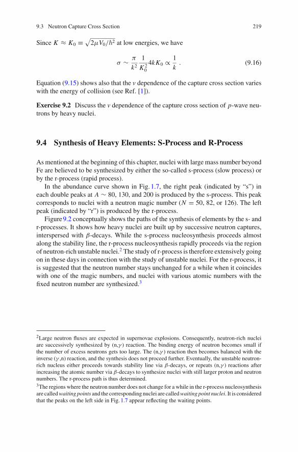
9.3 Neutron Capture Cross Section 219
Since K ≈ K0 ≡ √2μV0/�2 at low energies, we have
σ ∼ π
k21
K 20
4kK0 ∝ 1
k. (9.16)
Equation (9.15) shows also that the v dependence of the capture cross section varieswith the energy of collision (see Ref. [1]).
Exercise 9.2 Discuss the v dependence of the capture cross section of p-wave neu-trons by heavy nuclei.
9.4 Synthesis of Heavy Elements: S-Process and R-Process
Asmentioned at the beginning of this chapter, nuclei with large mass number beyondFe are believed to be synthesized by either the so-called s-process (slow process) orby the r-process (rapid process).
In the abundance curve shown in Fig. 1.7, the right peak (indicated by “s”) ineach double peaks at A ∼ 80, 130, and 200 is produced by the s-process. This peakcorresponds to nuclei with a neutron magic number (N = 50, 82, or 126). The leftpeak (indicated by “r”) is produced by the r-process.
Figure9.2 conceptually shows the paths of the synthesis of elements by the s- andr-processes. It shows how heavy nuclei are built up by successive neutron captures,interspersed with β-decays. While the s-process nucleosynthesis proceeds almostalong the stability line, the r-process nucleosynthesis rapidly proceeds via the regionof neutron-rich unstable nuclei.2 The study of r-process is therefore extensively goingon in these days in connection with the study of unstable nuclei. For the r-process, itis suggested that the neutron number stays unchanged for a while when it coincideswith one of the magic numbers, and nuclei with various atomic numbers with thefixed neutron number are synthesized.3
2Large neutron fluxes are expected in supernovae explosions. Consequently, neutron-rich nucleiare successively synthesized by (n,γ ) reaction. The binding energy of neutron becomes small ifthe number of excess neutrons gets too large. The (n,γ ) reaction then becomes balanced with theinverse (γ ,n) reaction, and the synthesis does not proceed further. Eventually, the unstable neutron-rich nucleus either proceeds towards stability line via β-decays, or repeats (n,γ ) reactions afterincreasing the atomic number via β-decays to synthesize nuclei with still larger proton and neutronnumbers. The r-process path is thus determined.3The regions where the neutron number does not change for a while in the r-process nucleosynthesisare calledwaiting points and the corresponding nuclei are calledwaiting point nuclei. It is consideredthat the peaks on the left side in Fig. 1.7 appear reflecting the waiting points.
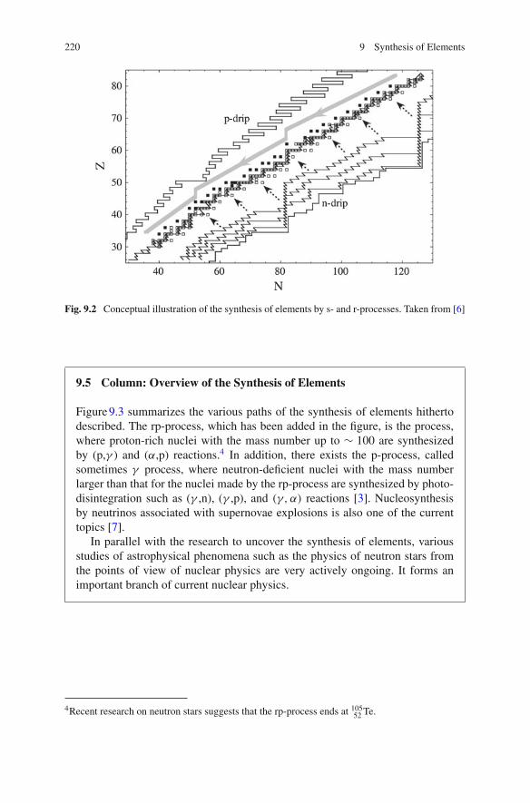
220 9 Synthesis of Elements
Fig. 9.2 Conceptual illustration of the synthesis of elements by s- and r-processes. Taken from [6]
9.5 Column: Overview of the Synthesis of Elements
Figure9.3 summarizes the various paths of the synthesis of elements hithertodescribed. The rp-process, which has been added in the figure, is the process,where proton-rich nuclei with the mass number up to ∼ 100 are synthesizedby (p,γ ) and (α,p) reactions.4 In addition, there exists the p-process, calledsometimes γ process, where neutron-deficient nuclei with the mass numberlarger than that for the nuclei made by the rp-process are synthesized by photo-disintegration such as (γ ,n), (γ ,p), and (γ, α) reactions [3]. Nucleosynthesisby neutrinos associated with supernovae explosions is also one of the currenttopics [7].
In parallel with the research to uncover the synthesis of elements, variousstudies of astrophysical phenomena such as the physics of neutron stars fromthe points of view of nuclear physics are very actively ongoing. It forms animportant branch of current nuclear physics.
4Recent research on neutron stars suggests that the rp-process ends at 10552 Te.
9.5 Column: Overview of the Synthesis of Elements 221
Fig. 9.3 Paths of nucleosynthesis. After [4] with some modifications
References
1. D.D. Clayton, Principles of Stellar Evolution and Nucleosynthesis (The University of ChicagoPress, Chicago, 1968)
2. C.E. Rolfs, W.S. Rodney, Cauldrons in the Cosmos (The University of Chicago Press, Chicago,1988)
3. I.J. Thompson, F.M. Nunes, Nuclear Reactions for Astrophysics: Principles, Calculation andApplications of Low-Energy Reactions (Cambridge University Press, Cambridge, 2009)
4. VHS Element Genesis—Solving the Mystery, Sci. Eds. Y. Motizuki, I. Tanihata, Y. Yano, R.Boyd (RIKEN & Image Science, Inc., 2001)
5. M. Junker et al., Phys. Rev. C 57, 2700 (1998)6. M. Arnould, S. Goriely, K. Takahashi, Phys. Rep. 450, 97 (2007)7. J.N. Bahcall, Neutrino Astrophysics (Cambridge University Press, Cambridge, 1989)
Appendix AImportant Formulae and Their Derivation
Abstract This chapter collects appendices to the previous chapters.
A.1 Basics of Scattering Problems
Here we summarize some basics for scattering problems such as the partial waveexpansion of the scattering amplitude.1
A.1.1 Partial Wave Expansion
(1) The asymptotic form of the radial wave function for the partial wave � (the caseof a short range force; k is the incident wave number, S is the scattering matrix,i.e., the S-matrix, and δ is the phase shift)
R�(r) ∼ 1
kr
[e−i(kr− 1
2 �π) − S(�)ei(kr− 12 �π)
](A.1)
∼ 1
krsin
(kr − 1
2�π + δ�
). (A.2)
(2) Partial wave expansion of the elastic scattering amplitude2 (θ is the scatteringangle, and α is the index of each state)
1We consider the scattering of particles without spin. See [1] for the scattering of particles withspin.2When one takes the partial wave sum in the case of the scattering problem involving Coulombforce, it is traditional to separate out the Rutherford scattering amplitude.
© Springer Japan 2017N. Takigawa and K. Washiyama, Fundamentals of Nuclear Physics,DOI 10.1007/978-4-431-55378-6
223
224 Appendix A: Important Formulae and Their Derivation
f (el)(θ) = 1
2ik
∞∑�=0
(2� + 1)(Sα,α(�) − 1
)P�(cos θ) , (A.3)
Sα,α(�) = e2iδ� . (A.4)
(3) Partial wave expansion of the inelastic scattering amplitude (α and β are thestate indices)
f (inel)β �=α (θ) = 1
2ik
∑�
(2� + 1) Sβ,α(�)P�(cos θ) . (A.5)
(4) Cross sections of the elastic, inelastic and total inelastic scattering
σ (el) =∑
�
σ(el)� = π
k2α
∑�
(2� + 1)|Sα,α(�) − 1|2 , (A.6)
σ(inel)β �=α =
∑�
σ(inel)β �=α (�) = π
k2α
∑�
(2� + 1)|Sβ,α(�)|2 , (A.7)
σ (inel) =∑β �=α
σ(inel)β �=α = π
k2α
∑�
(2� + 1)[1 − |Sα,α(�)|2] , (A.8)
(5) Unitarity condition ∑β
|Sβ,α(�)|2 = 1 . (A.9)
(6) Total cross section (ReS is the real part of the S-matrix)
σ (total) = σ (el) + σ (inel) = 2π
k2α
∑�
(2� + 1)(1 − ReS) . (A.10)
(7) Optical theorem (Im f (el) is the imaginary part of f (el))
σ (total) = 4π
kα
Im f (el)(θ = 0) . (A.11)
A.1.2 Sommerfeld–Watson Transformation
For high energy scattering, it is more convenient to use the integral representationof the scattering amplitude instead of the partial wave expansion. The integral repre-sentation sometimes becomes useful for scattering at low energies as well. Startingfrom the integral representation of the scattering amplitude and deriving character-istic closed form expression through some suitable approximation scheme such asthe stationary phase approximation or the method of steepest descent, one can often
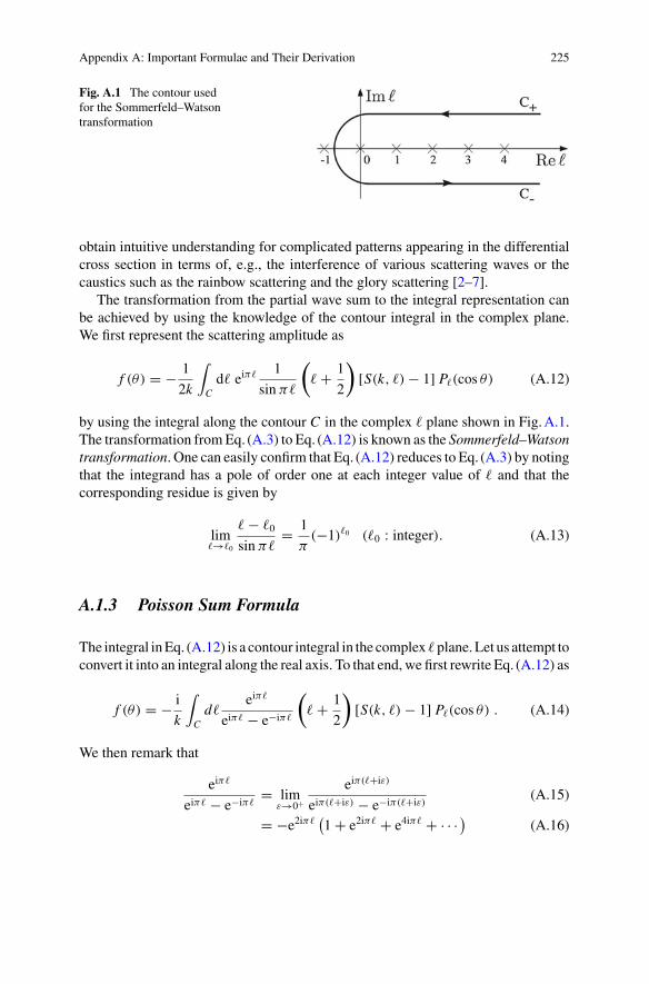
Appendix A: Important Formulae and Their Derivation 225
Fig. A.1 The contour usedfor the Sommerfeld–Watsontransformation
obtain intuitive understanding for complicated patterns appearing in the differentialcross section in terms of, e.g., the interference of various scattering waves or thecaustics such as the rainbow scattering and the glory scattering [2–7].
The transformation from the partial wave sum to the integral representation canbe achieved by using the knowledge of the contour integral in the complex plane.We first represent the scattering amplitude as
f (θ) = − 1
2k
∫Cd� eiπ� 1
sin π�
(� + 1
2
)[S(k, �) − 1] P�(cos θ) (A.12)
by using the integral along the contour C in the complex � plane shown in Fig.A.1.The transformation fromEq. (A.3) to Eq. (A.12) is known as the Sommerfeld–Watsontransformation. One can easily confirm that Eq. (A.12) reduces to Eq. (A.3) by notingthat the integrand has a pole of order one at each integer value of � and that thecorresponding residue is given by
lim�→�0
� − �0
sin π�= 1
π(−1)�0 (�0 : integer). (A.13)
A.1.3 Poisson Sum Formula
The integral inEq. (A.12) is a contour integral in the complex �plane.Let us attempt toconvert it into an integral along the real axis. To that end, we first rewrite Eq. (A.12) as
f (θ) = − i
k
∫C
d�eiπ�
eiπ� − e−iπ�
(� + 1
2
)[S(k, �) − 1] P�(cos θ) . (A.14)
We then remark that
eiπ�
eiπ� − e−iπ�= lim
ε→0+
eiπ(�+iε)
eiπ(�+iε) − e−iπ(�+iε)(A.15)
= −e2iπ�(1 + e2iπ� + e4iπ� + · · · )
(A.16)
226 Appendix A: Important Formulae and Their Derivation
on the contour C+ above the real axis, and that
eiπ�
eiπ� − e−iπ�= lim
ε→0+
eiπ(�−iε)
eiπ(�−iε) − e−iπ(�−iε)(A.17)
= 1 + e−2iπ� + e−4iπ� + · · · (A.18)
on the contour C− below the real axis, hence
∫Cd�
eiπ�
eiπ� − e−iπ�h(�) =
(∫C+
+∫
C−
)d�
eiπ�
eiπ� − e−iπ�h(�)
=∞∑
m=−∞
∫ ∞
−1/2d� e2iπm�h(�) , (A.19)
for a function h(�). We finally obtain
f (k, θ) = − i
k
∞∑m=−∞
(−1)m∫ ∞
0dλe2π imλλ [S(k, λ − 1/2) − 1] Pλ−1/2(cos θ)
(A.20)by introducing the Langer replacement � + 1/2 = λ, which is referred to also as theLanger correction or the Langer modification. Equation (A.20) is called the Poissonsum formula. In the semi-classical theory for scattering [8], m represents the numberof times which the incident particle circulates the target particle. The m = 0 termgoverns the scattering at high energies or if the attractive force between the projectileand target particles is weak. However, the m ≥ 1 terms also play important roles inthe scattering at low energies if a strong attractive force is involved [6].
We obtain the following Poisson sum formula for the cross section of the totalinelastic scattering by applying the similar procedure to Eq. (A.8),
σ (inel) = 2π
k2α
∞∑m=−∞
(−1)m∫ ∞
0dλe2iπmλλ
[1 − |Sα,α|2] (A.21)
= 2π∞∑
m=−∞(−1)m
∫ ∞
0db b e2iπmkb
[1 − |Sα,α(b)|2] (A.22)
≈ 2π∫ ∞
0db b
[1 − |Sα,α(b)|2] (for high energy). (A.23)
The relation between the angular momentum and the impact parameter λ = kb hasbeen used in transforming Eqs. (A.21) to (A.22).
Appendix A: Important Formulae and Their Derivation 227
A.2 Basics of Semi-classical Theory I: WKBApproximation
Here, let us first study theWKB approximation3 among various semi-classical meth-ods. The WKB approximation is the method to approximately obtain the solutionof the Schrödinger equation in the limit of taking the Planck constant � to be zero.Physically, it is valid when the change of the potential energy within a wave lengthcan be ignored compared with the magnitude of the local kinetic energy. Hence, itcan be said to be a short wave length approximation. In this approximation, the wavefunction and the phase shift as well as the scattering matrix for scattering problemsare given in terms of the action integrals in classical mechanics.
A.2.1 Wave Function
As an example, let us consider a problem where the potential is given by Vn(r) +VC(r), the former and the latter being the nuclear and the Coulomb potentials, re-spectively, and approximately obtain ψ�(r) when the radial wave function R�(r) ofan eigenstate of energy or the scattering problem with the orbital angular momentum� is expressed as R�(r) ≡ ψ�(r)/r . The ψ�(r) obeys the following equation:
[− �
2
2μ
d2
dr2+ V (r) − E
]ψ�(r) = 0 , (A.24)
V (r) = Vn(r) + VC(r) + V�(r) , (A.25)
V�(r) = �2
2μ
(� + 1/2)2
r2= �
2
2μ
λ2
r2. (A.26)
We introduced the Langer replacement �(� + 1) → (� + 1/2)2 ≡ λ2 in Eq. (A.26).In the WKB approximation, we express the wave function in the form of the
product of the amplitude and the phase factor, and write
ψ(r) = A(r)eiS(r)/� . (A.27)
We leave out the index � in Eq. (A.27) and throughout this section. Making thesubstitution Eq. (A.27) in Eq. (A.24) and treating A(r), S(r) and V (r) as quantitiesindependent of � and collecting the terms with the same powers of �, we obtain
3Wenzel–Kramers–Brillion approximation. It is also called the JWKB approximation by includingthe name of Jefferey.
228 Appendix A: Important Formulae and Their Derivation
[1
2μ
(dS
dr
)2
+ V (r) − E
]A�
0 − i
2μ
[2dA
dr
dS
dr+ A
d2S
dr2
]�1 − 1
2μ
d2 A
dr2�2 = 0 .
(A.28)By considering the limit of � → 0, and setting the coefficients of the zeroth and thefirst order power of � to be zero separately, we obtain
[1
2μ
(dS
dr
)2
+ V (r) − E
]= 0 , (A.29)
d
dr
(A2 dS
dr
)= 0 . (A.30)
Equation (A.29) corresponds to theHamilton–Jacobi equation in classicalmechanics,and suggests that S is given by the action integral in classical mechanics
S = ±∫ √
2μ(E − V (r))dr = ±�
∫k(r)dr . (A.31)
Equation (A.30) denotes the conservation of the current density. Together withEq. (A.31), it shows that the amplitude A is inversely proportional to the squareroot of the wave number, i.e.,
A ∝ 1√k(r)
. (A.32)
Finally, the wave function is given by
ψ(r) = A+1√k(r)
exp
(i∫ r
r0
k(r ′)dr ′)
+ A−1√k(r)
exp
(−i
∫ r
r0
k(r ′)dr ′)
,
(A.33)where A+ and A− are constants. In this way, the wave function in the WKB approx-imation is given by replacing the wave number times displacement in the argumentsof the exponential functions for a free particle with the action integral using the localwave number. This is a natural consequence, since the WKB approximation is basedon the assumption that the spatial change of momentum is small.
The �2 term in Eq. (A.28) has to be sufficiently small compared with the other
terms in order for the WKB approximation to be applicable. Equations (A.31) and(A.32) lead to
d2 A
dr2
/[A
�2
(dS
dr
)2]∼ 3
16
1
(�2k2(r)/2μ)2
1
k2(r)
(dV
dr
)2
+ · · · . (A.34)
Thus, the condition for the WKB approximation to be valid is that the amount ofchange of the potential energy within a wave length is much smaller than the kineticenergy at that position.
Appendix A: Important Formulae and Their Derivation 229
A.3 Basics of Semi-Classical Theory II: Methodof Comparison Equation
In this section, we formulate the semi-classical theory, i.e., the WKB method, usingthe method of comparison equation, which is different from the standard methoddescribed in Sect.A.2.
A.3.1 Principle of the Method of Comparison Equation
Turning points play important roles in describing the reflection of a particle in clas-sical mechanics. Since the turning points are defined as the points where the energyof the particle matches the value of the potential energy, namely, as the points whereE = V (r), they become in general complex numbers if the potential is a complexpotential as in the case of scattering by an optical potential. There exist many turningpoints in the complex r plane even if V (r) is a real potential. For example, whenthe potential between the scattering nuclei has the form shown in Fig. 8.1, and whenthe scattering energy is slightly above the potential barrier, there appears a turningpoint, whose real part is the barrier position, at each side of, i.e., above and below,the real axis in the complex plane.
Exercise A.1 Let us express the potential near the barrier position rB as V (r) =VCB − μΩ2(r − rB)2/2 when the potential looks like Fig. 8.1. Discuss the changeof the positions of the classical turning points in the complex r plane as the scatteringenergy E varies from below to above the barrier height VCB.
We therefore make an analytic continuation of the Schrödinger equation to com-plex plane and seek the solution of the second order differential equation of a complexvariable r : [
d2
dr2+ χ(r)
]ψ(r) = 0 , (A.35)
χ(r) = 2μ
�2(E − V (r)) . (A.36)
V (r) can have in general both the real and the imaginary parts; V (r) = VR(r) +iVI (r), where both VR(r) and VI (r) are analytic functions and are real functionswhen r is real.
In the method of comparison equation, we introduce another space of a com-plex number, which we denote by σ , besides the complex r space, and introduce asubsidiary second order differential equation in that space:
[d2
dσ 2+ Γ (σ)
]φ(σ) = 0 , (A.37)
which is called the comparison equation.
230 Appendix A: Important Formulae and Their Derivation
The function Γ (σ) is chosen to have the same topological structure as that ofχ(r). In simpler words, it is chosen to have the same number of important zeropoints, that is, the same number of turning points. Moreover, it is so chosen thatthe exact solutions of Eq. (A.37) are functions whose properties are well known. Thebasic idea of the method of comparison equation is to obtain an approximate solutionψ(r) of the original Eq. (A.35) in terms of the solutions φ(σ) of Eq. (A.37), whoseproperties are well known, by introducing suitable comparison equation.
The mapping between the two spaces is made in the following way. We first mapthe important zeros in the r space onto the zeros in the σ space by one to onemapping,then define the mapping between the two spaces so that
dσ
dr=
[χ(r)
Γ (σ )
]1/2
. (A.38)
Since the integral form of Eq. (A.38) reads
∫ r
r0
[χ(r)]1/2 dr =∫ σ
σ0
[Γ (σ)]1/2 dσ , (A.39)
Equation (A.38) means that the mapping is made to conserve the action integral intwo spaces.
One can show that in this case it holds
ψ(r) ≈(dσ
dr
)−1/2
φ(σ(r)) (A.40)
in the limit of � → 0.In fact, by changing Eq. (A.40) into an identity equation, and inserting it into
Eq. (A.35), one obtains
(dσ
dr
)3/2[d2φ
dσ 2+ 1
�2Q(r)
(dσ
dr
)−2
φ(σ)
]+ f (σ )φ(σ ) = 0 , (A.41)
where
f (σ ) = −1
2
d
dr
[(dσ
dr
)−3/2 d2σ
dr2
]. (A.42)
In Eq. (A.41), we expressed as χ(r) = Q(r)/�2 in order to make the role of � clear.
Equation (A.41) shows that Eq. (A.37) is obtained in the limit of � → 0 if one definesthe mapping by Eq. (A.38). The error is given by ( dσdr )−3/2 f (σ )φ(σ )/
d2φ(σ)
dσ 2 .
Appendix A: Important Formulae and Their Derivation 231
A.3.2 Derivation of the WKB Wave Function
As a simple example, let us obtain the wave function at a place far from any classicalturning points. In this case, the Γ can be chosen as
Γ (σ) = 1 . (A.43)
The solution of the corresponding comparison Eq. (A.37) is given by
φ(σ) = Aeiσ + Be−iσ . (A.44)
On the other hand, Eq. (A.39) leads to
σ =∫
χ1/2dr =∫
k(r)dr . (A.45)
Since χ(r) = k2(r), we finally obtain
ψ(r) ∼ [χ(r)]−1/4
[A exp
(i∫ r
k(r ′)dr ′)
+ B exp
(−i
∫ r
k(r ′)dr ′)]
. (A.46)
The right-hand side agrees with Eq. (A.33) obtained in Sect.A.2, and is nothing butthe wave function in the WKB approximation.
Incidentally, the WKB formula for the tunneling probability can be derived byseparately treating the two turning points on both sides of the potential barrier as anisolated turning point, and using σ as Γ for each region, and connecting the wavefunctions on both sides by using the asymptotic form of the Airy function, whichis the corresponding φ. On the other hand, the formula of the barrier transmissionprobability in the uniform approximation (2.77) can be obtained by considering thepotential barrier basically as a parabolic barrier and hence by taking Γ = σ 2/4 − ε
and by studying the asymptotic behaviours of the corresponding eigenfunctions φ,which are the Whittaker functions [9, 10]. The ε is determined so as to conserve theaction integral between the two turning points at the potential barrier in the r andσ spaces. Also, the S matrix, which is the basis of Eqs. (8.5)–(8.8) can be derivedby mapping the inner region including r3 (see Fig. 8.1) by a linear function and thebarrier region by a quadratic function, determining approximate wave function foreach region and by connecting them using their asymptotic forms. In the connection,it is crucial to use the correct asymptotic forms of the Whittaker and Airy functionsdepending on the phase of the arguments.
232 Appendix A: Important Formulae and Their Derivation
A.4 Eikonal Approximation
A.4.1 Scattering Amplitude
The scattering amplitude by a potential V at high energies can be well given in theeikonal approximation as [11]
f (k, θ) = −ik∫ ∞
0db bJ0(kbθ)
[e2iΔ(b) − 1
], (A.47)
Δ(b) = δeikonal(�) = −m
2k�2
∫ +∞
−∞V (
√b2 + z2)dz , (A.48)
and the cross section as
σ(inel)eikonal ≈ 2π
∫ ∞
0db b
[1 − e−4ΔI (b)
](for high energy), (A.49)
ΔI (b) = ImΔ(b) . (A.50)
A.4.2 Glauber Theory
Here, we derive the formulae of the Glauber theory in the optical limit given byEqs. (2.34)–(2.37).
The starting point is Eqs. (A.47)–(A.49) of the eikonal approximation. In order toapply these equations to the nucleon–nucleus and nucleus–nucleus scattering, let usmicroscopically represent the scattering potential in terms of the sum of the nuclearforce between individual nucleons vN N (riP − r jT ),
V (R) =∑iP , jT
vN N (riP − r jT ) (A.51)
=∫∫
drPdrT vN N (rP − rT + R)ρP(rP)ρT (rT ) . (A.52)
In these equations,R is the coordinate of the relativemotion,R ≡ RP − RT , betweenthe centers of mass of the projectile and target nuclei, RP , RT . riP (r jT ) is thecoordinate of the i-th nucleon in the projectile ( j-th nucleon in the target) measuredfrom the origin of the space fixed coordinate system. rP and rT are the intrinsiccoordinates of the nucleons in the projectile and target nuclei measured fromRP andRT , respectively. ρP(rP) and ρT (rT ) are the nucleon densities of the projectile andtarget nuclei at rP and rT , respectively. In transforming from Eqs. (A.51) to (A.52),we used that the nucleon densities are given by ρP(rP) = ∑
iPδ(riP − RP − rP),
and ρT (rT ) = ∑jT
δ(r jT − RT − rT ), like Eq. (5.2). vN N (r) is the nuclear potential
Appendix A: Important Formulae and Their Derivation 233
between two nucleons, which are separated by r. The potential given by Eq. (A.52)is called the double folding potential, and is often used for the interaction betweentwo nuclei.
Since the nuclear force is of short range, we approximate it as
vN N (r) = (vRe + ivIm)δ(r). (A.53)
The imaginary part (ivIm) has been introduced to take into account the other processesthan the elastic scattering. The potential is then given by
V (R) = (vRe + ivIm)
∫drρP(r − R)ρT (r) . (A.54)
By inserting the result of Eq. (A.54) into Eq. (A.48) and using Eq. (A.49), we obtain
σ (inel) ≈ 2π∫ ∞
0db b
[1 − exp
(2μnn
knn�2vImOv(b)
)](for high energy) , (A.55)
where the overlap function Ov is given by Eq. (2.36). μnn and knn are the reducedmass and the wave number in the nucleus–nucleus scattering, respectively.
We next use the Born approximation and the optical theorem in order to relatethe strength of the nuclear force to the total cross section in the nucleon–nucleonscattering. By applying the formula in the Born approximation,
f (1)(θ) = − 1
4π
2m
�2
∫e−iq·rV (r)dr ,
to the nucleon–nucleon scattering, and assuming the limit of the short range forcegiven by Eq. (A.53), we obtain
fN N = − μN N
2π�2(vRe + ivIm) (A.56)
for the scattering amplitude fN N . μN N = MN /2 is the reduced mass in the nucleon–nucleon scattering. If we use here the optical theorem, we obtain
vIm = −2π�2
μN N
kN N
4πσ
(total)N N (kN N ) . (A.57)
kN N is the wave number of the relative motion in the nucleon–nucleon scattering,σ
(total)N N (kN N ) is the total cross section when the nucleon–nucleon collision takes place
at the wave number kN N . By inserting the results of Eq. (A.57) into Eq. (A.55), weobtain
σ (inel) ≈ 2π∫ ∞
0db b
[1 − exp
(−μnnkN N
knnμN Nσ
(total)N N (kN N )Ov(b)
)]. (A.58)
234 Appendix A: Important Formulae and Their Derivation
In order for Eq. (A.58) to agree with Eq. (2.34), it is required that
μnnkN N
knnμN N= 1 . (A.59)
This is equivalent to the condition (2.37). Equations (2.34)–(2.37) are derived in thisway. Since the proof used the same reaction cross section irrespective of the nucleonspecies, it will be adequate to use the average cross section σN N .
A.5 Non-local Potential
A characteristic of nuclear physics is that a non-local potential is often involved.The Fock potential in the Hartree–Fock approximation for nuclear structure, and theexchange potentials which appear when one microscopically describes the scatteringbetween complex nuclei such as the scattering between α particle and nucleus andbetween twoheavy nuclei by taking into account antisymmetrization amongnucleonsbased on, e.g., the resonating group method are typical examples.
On the other hand, one usually assumes a local potential for phenomenologicalanalyses of nuclear structure and nuclear reactions. In this section, we review somestandardmethods to convert the Schrödinger equation involving a non-local potential,hence an integro-differential equation, into an equivalent local differential equation,and interpret the characteristic effects due to non-locality in other physical terms, suchas the effective mass, which are relevant to the description by using local potential,hence by a local differential equation [1].
A.5.1 Integro-Differential Equation
We consider a one-dimensional problem and represent the local and the non-localpotentials byU and V , respectively. In this case, the wave function obeys the integro-differential equation:
− �2
2m
d2ψ(x)
dx2+ U (x)ψ(x) +
∫V (x, x ′)ψ(x ′)dx ′ = Eψ(x) . (A.60)
A.5.2 Equivalent Effective Local Potential: WKBApproximation
One useful method to study the characteristic physical effects of a non-local potentialis the method based on the WKB approximation. To that end, we first rewrite the
Appendix A: Important Formulae and Their Derivation 235
term of the non-local potential into
∫V (x, x ′)ψ(x ′)dx ′ =
∫V (x, x ′)e
i�
(x ′−x) pψdx ′ ψ(x) . (A.61)
The subscript ψ of the momentum operator p has been attached in order to indicatethat it operates on the wave function ψ . The essence of the WKB approximationis to represent the wave function in the form of a plane wave by using the localmomentum. Also, it is based on the assumption that the spatial variation of the wavenumber is small. Hence,
pψψ(x) ∼ p(x)ψ(x) , (A.62)
where p(x) is the local momentum at the position x .
A.5.2.1 WKB Approximation I: Local Momentum Approximation,Energy Dependent Potential
By applying the approximation (A.62) to Eq. (A.61), one obtains the following equiv-alent effective local potential:
Ueff(E; x) = U (x) +∫
V (x, x ′)ei�
(x ′−x)p(x)dx ′ (A.63)
= U (x) +∫
V (x, x ′)ei�
(x ′−x)√2m(E−Ueff (E;x))dx ′ (A.64)
∼ U (x) +∫
V (x, x ′)ei�
(x ′−x)√2m(E−U (x))dx ′ . (A.65)
Equation (A.65) is an approximate equation which is valid when the contributionfrom the non-local potential is small compared with U (x). As these formulae show,the equivalent effective local potential depends on the energy.
The energy dependence discussed here originates from non-locality. The potentialhas in addition another energy dependence due to the polarization or the channel-coupling effects such as the phonon excitation on the way of collision. The latter isoften called the intrinsic energy dependence in order to distinguish from the energydependence due to non-locality [1].
A.5.2.2 WKB Approximation II: Effective Mass
Let us next expand the translation operator exp[ i�(x ′ − x) pψ ] and keep up to the
second order terms,
exp
[i
�(x ′ − x) pψ
]≈ 1 + i
�(x ′ − x) pψ − 1
2!1
�2(x ′ − x)2 p2
ψ . (A.66)
236 Appendix A: Important Formulae and Their Derivation
Equation (A.60) is then approximated as
− �2
2meff
d2ψ(x)
dx2+ U (0)
eff (x)ψ(x) + V (1)(x)d
dxψ(x) = Eψ(x) , (A.67)
where
1
meff= 1
m− 1
�2
∫(x ′ − x)2V (x, x ′)dx ′ , (A.68)
U (0)eff (x) ≡ U (x) +
∫V (x, x ′)dx ′ , (A.69)
V (1)(x) ≡∫
(x ′ − x)V (x, x ′)dx ′ . (A.70)
In particular, suppose that the non-local potential is given by a separable type suchthat [12]
V (x, x ′) = F
(x + x ′
2
)G(x ′ − x) (A.71)
= F
(x + x ′
2
)1√π
1
λN Le−[(x ′−x)/λN L]2 (A.72)
∼ F(x)1√π
1
λN Le−[(x ′−x)/λN L]2 . (A.73)
λN L is a parameter to measure the degree of non-locality. The degree of non-localityis larger for larger values of λN L . Equation (A.73) leads to
1
meff(x)= 1
m− 1
�2F(x)
λ2N L
2, (A.74)
U (0)eff (x) ≡ U (x) + F(x) , (A.75)
V (1)(x) = 0 . (A.76)
Equation (A.74) indicates that Eq. (A.67) is valid when the degree of non-locality issmall, and that the mass parameter becomes position dependent due to the non-localpotential. In addition, Eq. (A.75) shows that the static part of the potential is alsomodified by the non-local potential.
A.5.2.3 WKB Approximation III: Wigner Transformation
Here we derive an alternative expression of the equivalent local potential based onthe Wigner transformation. Let us first rewrite the non-local potential term by usingthe Wigner transformation of the non-local potential as
Appendix A: Important Formulae and Their Derivation 237
∫V (x, x ′)ψ(x ′)dx ′
=[
1
2π�
∫dx ′
∫dpe−ip(x ′−x)/�ei(x ′−x) pV /2�VW (x, p)ei(x ′−x) pψ/�
]ψ(x) .
(A.77)
pV is an operator which operates on x in VW (x, p). If we assume
ei(x ′−x) pV /2�VW (x, p) ≈ VW (x, p) , (A.78)
we obtain∫
V (x, x ′)ψ(x ′)dx ′ = VW (x, pψ)ψ(x) (A.79)
∼ VW (x, p(x))ψ(x) . (A.80)
The local momentum approximation (A.62), which is based on the WKB approxi-mation, has been used in transforming from Eq. (A.79) to (A.80). Finally, we obtain
U (W )eff = U (x) + VW (x, p(x)) , (A.81)
for the equivalent effective local potential. The right-hand side of Eq. (A.81) agreeswith the equivalent potential in the phase space which appears in the classical theoryin the presence of a non-local potential [13].4
A.6 Tensor Algebra
A.6.1 Definition of Tensor Operators
The tensor property of a physical quantity or an operator represents their transfor-mation property under a rotation of either the coordinate system or the object and isa unified generalization of scalar, vector and tensor by introducing the index namedrank. The tensor property is one of the fundamental properties of each physical quan-tity like the spatial and/or temporal dimension related to units, and plays an importantrole, e.g., in evaluating transition matrices and in deriving selection rules.
4Thanks to the large effective mass and hence the short wave length property, the classical theorywhich uses the concept of classical trajectory is useful for heavy-ion collisions, and has beensuccessfully applied to analysing fusion reactions and deep inelastic collisions involving a hugeamount of energy dissipation from the relative motion to intrinsic motions and the associatedfluctuations [14, 15]. In that connection, it is an interesting question how to incorporate the exchangeeffects of nucleons in the classical theory. The semi-classical treatment of a non-local potential hasbeen discussed also in [16].
238 Appendix A: Important Formulae and Their Derivation
Let us consider a translation beforewe discuss a rotation. In that case, there are twoalternative ways. In the one, one keeps the object as it is, and performs a translationof the coordinate system from the old one K (x, y, z) to a new one K ′(x ′, y′, z′).In the other, one translates the object by keeping the coordinate system as it is. Here,we take the latter. Let us consider the translation of an object by a. If we express thewave function before and after the translation as ψ(x) and ψ ′(x), respectively, then
ψ ′(x) = ψ(x − a)
= ψ(x) − ad
dxψ(x) + 1
2!d2
dx2ψ(x) + · · ·
= e−ia �
iddx /�ψ(x) = e−ia p/�ψ(x) . (A.82)
Equation (A.82) shows that p is the generator of the infinitesimal translation in space.Equation (A.82) is expressed as
|ψ ′〉 = T (a)|ψ〉 , (A.83)
T (a) ≡ e−ia p/� , (A.84)
in the Dirac notation. T (a) given by Eq. (A.84) is the unitary operator which causesthe translation by a.5 Also, if we define the operator O ′ for an operator O repre-senting some observable in such a way that the expectation value is conserved undertransformation, namely, by
〈ψ |O|ψ〉 ≡ 〈ψ ′|O ′|ψ ′〉 , (A.85)
then by rewriting the right-hand side of Eq. (A.85) as 〈ψ ′|O ′|ψ ′〉 = 〈ψ |T † O ′T |ψ〉,we find that O ′ is given by
O ′ = T (a)O T †(a) = T (a)O T −1(a) . (A.86)
Equation (A.86) shows that the operator is transformed by the same unitary operatoras that for the state vector ψ .
Exercise A.2 Show
x ′ ≡ T (a)x T †(a) = x − a , (A.87)
〈ψ ′|x |ψ ′〉 = 〈ψ |x |ψ〉 + a , (A.88)
by using Eq. (A.84). Equation (A.88) agrees with that |ψ ′〉 is the state, where theobject is translated by a.
5It is the operator to cause the translation by −a if one takes the point of view of fixing the objectand transforming the coordinate system.
Appendix A: Important Formulae and Their Derivation 239
Analogously, by considering infinitesimal rotations, one can show that the gen-erators of the infinitesimal rotations are the angular momentum operators Jα (α =x, y, z). For example, the rotation of an object through an angle α about the z-axisis given by the unitary operator Rz = e−iα Jz . By extending this result, the unitaryoperator for a rotation in the three-dimensional space is in general given either as
R(w) = e−iw·J (A.89)
by using the vector w, which specifies the direction and the magnitude of rotation,or as
R(φ, θ, ψ) = e−iφ Jze−iθ Jye−iψ Jz (A.90)
by using the Euler angles [17].
(i) First Definition of a Tensor Operator: When 2k + 1 operators T (k)q (q =
−k,−k + 1, . . . , k − 1, k) transform to each other following
(T (k)q )′ = RT (k)
q R−1 =k∑
q ′=−k
T (k)q ′ R(k)
q ′q(φ, θ, ψ) (A.91)
under a rotation, T (k) is called an irreducible tensor of rank k, and T (k)q the q-
component. The rotation matrix R(k)q ′q(φ, θ, ψ) is defined by
R(k)q ′q(φ, θ, ψ) ≡ 〈kq ′|R(φ, θ, ψ)|kq〉 . (A.92)
[N.B.] Equation (A.92) obeys [17]. It is the same as D function in Ref. [18]:R(k)
q ′q(φ, θ, ψ) = (D(k)q ′q(φ, θ, ψ))BS. It is related to the D function in Ref. [19] as
R(k)q ′q(φ, θ, ψ) = (D (k) ∗
q ′q (φ, θ, ψ))BM. Since Ref. [20] transforms coordinate systemrather than the object, the sign of the arguments of the D function is inverted:R(k)
q ′q(φ, θ, ψ) = (D (k)q ′q(−φ,−θ,−ψ))RS. In this book, the definition ofD
(k)qq ′ follows
Ref. [19].
(ii) Second Definition of a Tensor Operator: Since the generators of the infini-tesimal rotations are the angular momentum operators, one can alternatively definethe irreducible tensor of rank k as the set of operators which satisfy the followingcommutation relations:
[Jz, T (k)
q
]= qT (k)
q , (A.93)[J±, T (k)
q
]= √
(k ∓ q)(k ± q + 1)T (k)q±1 . (A.94)
In order to show the equivalence between the two definitions, we show here thatEqs. (A.93) and (A.94) can be derived from Eq. (A.91). Let us now assume that Ris the infinitesimal rotation operator (1 − iα Jλ). In this case, from the definition
240 Appendix A: Important Formulae and Their Derivation
Eq. (A.92), we have
R(k)q ′q = 〈kq ′|(1 − iα Jλ)|kq〉 = δq ′q − iα〈kq ′| Jλ|kq〉 . (A.95)
On the other hand,
RT (k)q R−1 = (1 − iα Jλ)T
(k)q (1 + iα Jλ) . (A.96)
Hence from Eq. (A.91)
(1 − iα Jλ)T(k)
q (1 + iα Jλ) =(δq ′q − iα〈kq ′| Jλ|kq〉
)T (k)
q ′ . (A.97)
Thus it follows[ Jλ, T (k)
q ] =∑
q ′〈kq ′| Jλ|kq〉T (k)
q ′ . (A.98)
By putting here Jλ = Jz and Jλ = J± and noting
〈kq ′| Jz|kq〉 = qδq ′q , 〈k q ± 1| J±|kq〉 = √(k ∓ q)(k ± q + 1) , (A.99)
we obtain Eqs. (A.93) and (A.94).
A.6.2 Examples of Irreducible Tensor
(i) Spherical Harmonics: Ykq(θ, ϕ).
(ii) Tensor of Rank 1: Vector Operators A vector is an irreducible tensor of rank1 and its 1, 0,−1 and x, y, z components are related as [18],
V±1 = ∓ 1√2(Vx ± iVy) ,
V0 = Vz . (A.100)
Equation (A.100) can be understood from the fact that the x , y and z components ofthe position vector r can be expressed as
rY1±1 = ∓√
3
4π
1√2(x ± iy) ,
rY10 =√
3
4πz , (A.101)
by using the explicit expressions of the irreducible tensor of rank 1, Y1q .
Appendix A: Important Formulae and Their Derivation 241
A.6.3 Wigner–Eckart Theorem
The following formula holds6
〈α J M |T (k)q |α′ J ′M ′〉 = 1√
2J + 1〈J ′k M ′q|J M〉〈α J‖T (k)‖α′ J ′〉 , (A.102)
for the q component of a tensor of rank k, T (k)q . Theα andα′ are the quantum numbers
other than the angular momentum to specify states.Equation (A.102) is called the Wigner–Eckart theorem, and shows that the matrix
element of a tensor operator can factor out the dependence on the z-component of theangular momentum in terms of the geometrical factor given by the Clebsch–Gordancoefficient. The factor 〈α J‖T (k)‖α′ J ′〉 is called the reduced matrix element. TheWigner–Eckart theorem allows to automatically determine all the matrix elementsbased on the Clebsch–Gordan coefficient if the reducedmatrix element is once deter-mined by calculating the matrix element for one combination of M ′, q, M for whichthe Clebsch–Gordan coefficient is finite.
Especially when T is 1 or the angular momentum operators or the sphericalharmonics, the reduced matrix elements are given by
〈α J‖1‖α′ J ′〉 = δαα′δJ J ′√2J + 1 , (A.103)
〈α J‖J‖α′ J ′〉 = δαα′δJ J ′√
J (J + 1)(2J + 1) (A.104)
〈�‖Y (k)‖�′〉 = (−1)�−�′−k
√(2k + 1)(2�′ + 1)
4π〈k�′00|�0〉
= (−1)�√
(2k + 1)(2�′ + 1)(2� + 1)
4π
(� k �′0 0 0
), (A.105)
where
(� k �′0 0 0
)is a 3 j symbol.
A.6.4 Projection Theorem
Using the Wigner–Eckart theorem, one can show that the matrix element of anyvector operator A can be expressed as
〈α J M |A|α J M ′〉 = 1
J (J + 1)〈α J M |J|α J M ′〉〈α J J |(A · J)|α J J 〉 . (A.106)
6There exists an alternative definition, which does not explicitly take out the factor 1/√2J + 1 on
the right-hand side, but includes it in the factor 〈α J‖T ‖α′ J ′〉.
242 Appendix A: Important Formulae and Their Derivation
Equation (A.106) is called the projection theorem or the Landé formula, and is use-ful, e.g., in deriving the Schmidt values for the magnetic dipole moment given inSect. 5.4.1.
A.6.5 Relation Between the Scalar Product and the TensorProduct of Rank 0
One can define a combined tensor operator of two tensor operators by taking anappropriate sum of the product of their components using the Clebsch–Gordancoefficients as follows
V (K )Q ≡ [
T (k1) × U (k2)](K )
Q ≡∑
q1
〈k1k2q1q2|K Q〉T (k1)q1 U (k2)
q2 . (A.107)
In the case of a combined tensor of rank 0, one can use the scalar product definedby
S ≡ (T (k) · U (k)) ≡∑
q
(−1)q T (k)q U (k)
−q (scalar product), (A.108)
for V (0)0 . Especially, the scalar product of two vectors is given by
S = (V(1) · W(1)) = Vx Wx + Vy Wy + Vz Wz . (A.109)
Exercise A.3 Show that the scalar product and the tensor of rank 0 are related as
S = (−1)k√2k + 1 V (0)
0 (A.110)
when one combines two tensors of rank k.
A.7 Relation Between the Quadrupole Momentand Intrinsic Quadrupole Moment
Here, we prove Eq. (4.47), which relates the experimentally observed quadrupolemoment for a deformed nucleus to the intrinsic quadrupole moment.
We first remark from the general transformation formula of a tensor, Eq. (A.91),that the multipole moment operator Qintr.
λμ given by the intrinsic coordinates and the
corresponding operator Qlab.λμ which is related to the experimental measurement and
is defined by the coordinates in the laboratory system are related as
Appendix A: Important Formulae and Their Derivation 243
Qintr.λμ =
∑μ′
Dλ∗μ′μ(ω)Qlab.
λμ′ , Qlab.λμ =
∑ν
Dλμν(ω)Qintr.
λν , (A.111)
through the Euler anglesω = (φ, θ, ψ)which specify the orientation of the principalaxes. We used the properties of the D function in transforming from the first to thesecond equations. Since the wave function for an axial-symmetrically deformed stateis given by Eq. (8.72), the matrix element of the operator is given in general by
⟨ΨI1M1K1
∣∣∣Qlab.λμ
∣∣∣ ΨI2M2K2
⟩=
∑ν
(2I1 + 1
16π2(1 + δK10)
)1/2 (2I2 + 1
16π2(1 + δK20)
)1/2
×[⟨D I1
M1K1
∣∣Dλμν
∣∣D I2M2K2
⟩ ⟨ΦK1
∣∣∣Qintr.λν
∣∣∣ ΦK2
⟩
+ (−1)I2+K2
⟨D I1
M1K1
∣∣Dλμν
∣∣D I2M2−K2
⟩ ⟨ΦK1
∣∣∣Qintr.λν
∣∣∣ ΦK2
⟩
+ (−1)I1+K1
⟨D I1
M1−K1
∣∣Dλμν
∣∣D I2M2K2
⟩ ⟨ΦK1
∣∣∣Qintr.λν
∣∣∣ ΦK2
⟩
+ (−1)I2+K2+I1+K1
⟨D I1
M1−K1
∣∣Dλμν
∣∣D I2M2−K2
⟩ ⟨ΦK1
∣∣∣Qintr.λν
∣∣∣ ΦK2
⟩]. (A.112)
In the following, we consider the quadrupole moment. Since the quadrupole mo-ment is defined by 〈ΨI M=I K |Qlab.
λ=2,μ=0|ΨI M=I K 〉, one can easily show that the secondand third terms on the right-hand side of Eq. (A.112) are zero for axial-symmetricallydeformed even–even nuclei7 and for odd nuclei in the strong coupling state withI = K = 1/2 or K ≥ 3/2 by noting the properties of the D function, |ν| ≤ 2, theaddition rule of two angular momenta and the fact that K = 0, 2, 4 · · · for collectivemotions of axial-symmetrically deformed even–even nuclei. In addition, the fourthand first terms become equal. It therefore follows
〈ΨI I K |Qlab.20 |ΨI I K 〉 =
∑ν
2I + 1
8π2〈D I
M=I K |D20ν |D I
M=I K 〉〈ΦK |Qintr.λν |ΦK 〉 (A.113)
= 〈2I0I |I I 〉〈2I0K |I K 〉〈ΦK |Qintr.20 |ΦK 〉 . (A.114)
We then obtain Eq. (4.47) by using the explicit expression of the Clebsch–Gordancoefficient.
A.8 Derivation of the Formula for the α-Decay WidthBased on the Gamow Model: Direct Method
Here, we derive the formulae (8.13)–(8.17) for the α-decay width. We first note thatin the Gamow model the wave function is given by
7This excludes the case when K1 = K2 = 0. The second and third terms can be combined with thefirst and/or fourth terms when K1 = K2 = 0.
244 Appendix A: Important Formulae and Their Derivation
φ(r) ={
φI (r) = N j0(Kr) for r < R
φI I (r) = (μ/�k)1/2 [G0(η, kr) + iF0(η, kr)] /r for r ≥ R ,(A.115)
where K and k = kα are given by Eq. (8.17). The continuity conditions at r = Rrequire that
N sin KR =√
μ
�kK [G0(η, k R) + iF0(η, k R)]
N cos KR =√
μ
�kk
[G ′
0(η, k R) + iF ′0(η, k R)
], (A.116)
where G ′0 and F ′
0 are the derivative of G0(η, ρ) and F0(η, ρ)with respect to ρ, whereρ = kr . These equations lead to
k
Ktan KR = G0(η, k R) + iF0(η, k R)
G ′0(η, k R) + iF ′
0(η, k R). (A.117)
On the other hand, the decay width Γ is given by the outgoing flux per unit time atthe external turning point of the potential barrier in the case when the wave functioninside the potential is normalized to be unity,
Γ
�≡ flux at the external turning point
probability to be inside the potential. (A.118)
Since Eq. (A.115) normalizes the external flux to be unity, we have
�
Γ=
∫ R
0|φI (r)|2r2dr +
∫ re
R|φI I (r)|2r2dr (A.119)
= μ
�k2
[1
2k R
G20(η, k R) + F2
0 (η, k R)
sin2 KR
(1 − sin 2KR
2KR
)
+∫ 2η
k R(G2
0(η, ρ) + F20 (η, ρ))dρ
]. (A.120)
One can determine the energy E , i.e., the Q-value for the α-decay, and the decaywidth Γ by using Eqs. (A.117) and (A.120) if the depth of the potential V0 and therange of the nuclear force R are known in advance. Conversely, one can determinethe depth of the potential V0 and the range of the nuclear force R for the α-decay fromthe Q-value and the decay width using Eqs. (A.117) and (A.120) if they are knownexperimentally. However, as discussed in Sect. 8.1.1, there remains an ambiguity ofpotential because of the presence of Pauli forbidden states, in other words, redundantstates. In order to remove the ambiguity, one needs to specify the number of nodes inthewave function for the relativemotion. As one example of such analyses, TableA.1
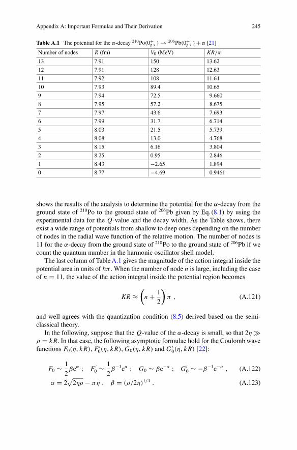
Appendix A: Important Formulae and Their Derivation 245
Table A.1 The potential for the α-decay 210Po(0+g.s.) → 206Pb(0+
g.s.) + α [21]
Number of nodes R (fm) V0 (MeV) KR/π
13 7.91 150 13.62
12 7.91 128 12.63
11 7.92 108 11.64
10 7.93 89.4 10.65
9 7.94 72.5 9.660
8 7.95 57.2 8.675
7 7.97 43.6 7.693
6 7.99 31.7 6.714
5 8.03 21.5 5.739
4 8.08 13.0 4.768
3 8.15 6.16 3.804
2 8.25 0.95 2.846
1 8.43 −2.65 1.894
0 8.77 −4.69 0.9461
shows the results of the analysis to determine the potential for the α-decay from theground state of 210Po to the ground state of 206Pb given by Eq. (8.1) by using theexperimental data for the Q-value and the decay width. As the Table shows, thereexist a wide range of potentials from shallow to deep ones depending on the numberof nodes in the radial wave function of the relative motion. The number of nodes is11 for the α-decay from the ground state of 210Po to the ground state of 206Pb if wecount the quantum number in the harmonic oscillator shell model.
The last column of TableA.1 gives the magnitude of the action integral inside thepotential area in units of �π . When the number of node n is large, including the caseof n = 11, the value of the action integral inside the potential region becomes
KR ≈(
n + 1
2
)π , (A.121)
and well agrees with the quantization condition (8.5) derived based on the semi-classical theory.
In the following, suppose that the Q-value of the α-decay is small, so that 2η �ρ = k R. In that case, the following asymptotic formulae hold for the Coulomb wavefunctions F0(η, k R), F ′
0(η, k R), G0(η, k R) and G ′0(η, k R) [22]:
F0 ∼ 1
2βeα ; F ′
0 ∼ 1
2β−1eα ; G0 ∼ βe−α ; G ′
0 ∼ −β−1e−α , (A.122)
α = 2√2ηρ − πη , β = (ρ/2η)1/4 . (A.123)
246 Appendix A: Important Formulae and Their Derivation
Let us now relate the decaywidth to the tunneling probability byusingEq. (A.121).We set sin 2KR to 0 based on Eq. (A.121). Equations (A.122) and (A.123) suggest|F0(η, k R)| � |G0(η, k R)|, so that we can ignore F0 in Eq. (A.120). Also, we ignorethe integration term as well. The decay width is then approximately given by
Γ ∼ 2�2k
μR
1
G20(η, k R)
. (A.124)
On the other hand, the tunneling probability t is given by the ratio of the outgoingflux J (+)
I I to the flux J (+)I which enters the potential barrier at r = R in the outward
direction from inside. Since J (+)I and J (+)
I I are given by
J (+)I =
∫j (+)I dS =
∫1
r2�K
μ
∣∣∣∣ N
2K
∣∣∣∣2
r2dΩ = 4π�K
μ
∣∣∣∣ N
2K
∣∣∣∣2
, (A.125)
J (+)I I =
∫j (+)I I dS =
∫1
r2r2dΩ = 4π , (A.126)
the tunneling probability becomes
t (D)GM ≡ J (+)
I I
J (+)I
∼ 4k
K
sin2 KR
G20(η, k R)
∼ 4k
K
1
G20(η, k R)
. (A.127)
Equations (A.124) and (A.127) lead to Eq. (8.13).Thus one can obtain Eqs. (8.13)–(8.17) by using the asymptotic forms of the
Coulomb wave functions given by Eqs. (A.122) and (A.123) [22], which hold whenk R � 2η = kre, i.e., when R � re or when the Q-value is small.
A.9 Basics of Electromagnetic Transitions
A.9.1 Hamiltonian of the Total System
To discuss the electromagnetic transitions of a nucleus, it is necessary to treat thecombined system consisting of the nucleus, i.e., a many-body system of nucleons,and the electromagnetic fields. The Hamiltonian of the total system is given by
Htot = Hnucl + Hfield + Hint . (A.128)
Hnucl is the Hamiltonian of an isolated nucleus, and consists of the kinetic energy ofnucleons and the strong interaction among nucleons. Alternatively, it is expressedin an appropriate model such as the shell model or the collective model. We assumethat the eigenstates and the corresponding eigenvalues are known and express as
Appendix A: Important Formulae and Their Derivation 247
HnuclΨα = EαΨα . (A.129)
The Hamiltonian of the electromagnetic fields Hfield and the interaction Hamiltonianbetween the nucleus and the electromagnetic fields Hint are given by
Hfield = 1
8π
∫ [E2(r, t) + B2(r, t)
]dr , (A.130)
Hint = −1
c
∫jμ Aμdr (A.131)
=∫ [
ρ(r, t)Φ(r, t) − 1
cj(r, t)A(r, t)
]dr , (A.132)
where E, B, ρ and j are the electric field, the magnetic field, the charge and currentdensities of the nucleus, respectively.
From the point of view of the original many-body system of nucleons, ρ is givenby
ρ(r, t) =A∑
i=1
e
(1
2− t (i)
3
)δ(r − ri (t)) , (A.133)
while j byj(r, t) = c∇ × μ(r, t) (A.134)
using the magnetic moment μ(r, t). Since the magnetic moment originates from theorbital motion of protons, and also from the spins of protons and neutrons, j is givenby a sum of two parts. If we denote j originating from the orbital motion of protonsby jc, then
jc =A∑
i=1
e
(1
2− t (i)
3
)1
2[viδ(r − ri (t)) + h.c.] . (A.135)
vi is given by vi = i�
[Hnucl, ri
], and becomes vi = pi/MN if the potential in Hnucl
does not depend on the momentum. On the other hand, if we denote the magneticmoment originating from the spin of nucleons by μs , then it is given by
μs(r, t) =A∑
i=1
δ(r − ri (t))e�
2MN c
[(1
2− t (i)
3
)gp +
(1
2+ t (i)
3
)gn
]si (A.136)
using the g-factors of protons and neutrons: gp = 2.792847 × 2 ≈ 5.586, gn =−1.9130427 × 2 ≈ −3.826.
248 Appendix A: Important Formulae and Their Derivation
A.9.2 Wave Function of Photon: Vector SphericalHarmonics
A.9.2.1 Coulomb Gauge
It is convenient to adopt the Coulomb gauge, known also as the transverse gauge orthe radiation gauge [23]: ∇ · A = 0 (A.137)
in order to discuss the electromagnetic transitions. In this case, the Hamiltonian ofthe radiation field is given by
Hfield = 1
8π
∫ (1
c2A
2 + (∇ × A)2)dr , (A.138)
and the vector potential A obeys the wave equation:
ΔA − 1
c2∂2
∂t2A = 0 . (A.139)
If we put the time dependence as e−ickt , then we obtain the Helmholtz equation
(Δ + k2)A = 0 . (A.140)
Note that Eq. (A.137) indicates that the vector potential A is perpendicular to the di-rection of the propagation of thewave (k ⊥ A), i.e., that thewave is a transversewave.
A.9.2.2 Rotational Transformation of Vector Wave Functionand the Spin and Intrinsic Wave Function of Photon
When one uses the spherical polar coordinates andmakes the partial wave expansion,the solution of the Helmholtz equation (A.140) for the partial wave � is nothing butj�(kr) provided the field is a scalar field. In reality, photons are described by a vectorfield, so that they have spin 1 as we show later. It is therefore necessary to extend the
wave function so as to be a simultaneous eigenfunction of L2, S
2, J
2and Jz .
(i) The Transformation Property of a Vector Function: Let us first study how avector function V(r, θ, ϕ) is transformed under rotation. One needs to consider boththe transformation of vector components and that of coordinates under rotation. Forexample, when one rotates the coordinate system through α about the z-axis, thevector components in the new coordinate system are given by
⎛⎝V ′
x (r, θ, ϕ)
V ′y(r, θ, ϕ)
V ′z (r, θ, ϕ)
⎞⎠ =
⎛⎝ cosα sin α 0
− sin α cosα 00 0 1
⎞⎠
⎛⎝Vx (r, θ, ϕ + α)
Vy(r, θ, ϕ + α)
Vz(r, θ, ϕ + α)
⎞⎠ . (A.141)
Appendix A: Important Formulae and Their Derivation 249
For small α, Eq. (A.141) can be represented as
V′ = (1 + iα Jz)V + O(α2) , (A.142)
where Jz is given by
Jz = −i∂
∂ϕ+ iez × (A.143)
= −i
(x
∂
∂y− y
∂
∂x
)+ iez × (A.144)
= L z + iez × . (A.145)
ez × means to take the outer product between the unit vector in the z-axis ez and thevector V which appears on the right side in Eq. (A.142).
Exercise A.4 Prove Eq. (A.143) by noting that Eq. (A.141) leads to
V ′x (r, θ, ϕ) = Vx (r, θ, ϕ) + α
∂
∂ϕVx + αVy , (A.146)
V ′z (r, θ, ϕ) = Vz(r, θ, ϕ) + α
∂
∂ϕVz , (A.147)
and thatez × V = ey Vx − ex Vy . (A.148)
(ii) Spin of a Photon: Equation (A.145) shows that the intrinsic spin operator of aphoton is given by
Sx = iex × , Sy = iey × , Sz = iez × . (A.149)
Also, the total angular momentum is given by
J = L + S . (A.150)
Exercise A.5 Show that S defined byEq. (A.149) satisfies the commutation relationsof the angular momentum operator.
(iii) The Eigenvectors of the Intrinsic Spin of Photon: If we define
e+1 = − 1√2(ex + iey) ,
e0 = ez ,
e−1 = 1√2(ex − iey) , (A.151)
250 Appendix A: Important Formulae and Their Derivation
in terms of the unit vectors in the x, y, z direction by following the general rule thatrelates the 1, 0,−1 components of a tensor of rank 1 to the x, y, z components of avector, we can show that
S2eq = 2eq , Szeq = qeq (q = ±1, 0) . (A.152)
Equation (A.152) shows that the magnitude of the intrinsic spin of photon is 1 andthat the eigenvector corresponding to Sz = q is eq .
A.9.2.3 Vector Spherical Harmonics
(i) Definition: From the above arguments, it follows that thewave function of photon,
which is the simultaneous eigenfunction of L2, S
2, J
2and Jz , is given by
YJ�M(θ, ϕ) =∑mq
〈�1mq|J M〉Y�m(θ, ϕ)eq (A.153)
by using the addition rule of two angular momenta. YJ�M(θ, ϕ) are called vectorspherical harmonics.
One can easily show that the vector spherical harmonics have the following prop-erties,
J2YJ�M(θ, ϕ) = J (J + 1)YJ�M(θ, ϕ) , (A.154)
JzYJ�M(θ, ϕ) = MYJ�M(θ, ϕ) , (A.155)
L2YJ�M(θ, ϕ) = �(� + 1)YJ�M(θ, ϕ) , (A.156)
S2YJ�M(θ, ϕ) = 2YJ�M(θ, ϕ) , (A.157)
and the orthogonality,
∫dΩY∗
J�M(θ, ϕ) · YJ�M(θ, ϕ) = δJ J ′δ��′δM M ′ . (A.158)
Note that there exist three kinds of vector spherical harmonics YJ J M(θ, ϕ) andYJ J±1M (θ, ϕ), which have different values of the orbital angular momentum for eachset of J, M . They can be classified into the following two groups depending on thedifference of parity:
• YJ J M (θ, ϕ): Parity (−1)J
This corresponds to the magnetic field for the electric multipole radiation and tothe electric field for the magnetic multipole radiation.
Appendix A: Important Formulae and Their Derivation 251
• YJ J±1M (θ, ϕ): Parity (−1)J+1
This corresponds to the electric field for the electric multipole radiation and to themagnetic field for the magnetic multipole radiation.
(ii) The Method to Construct from the Ordinary Scalar Spherical Harmonics:The vector spherical harmonics can be constructed from the ordinary scalar sphericalharmonics by the following operations:
�Y�m(θ, ϕ) = √�(� + 1)Y��m(θ, ϕ) , (A.159)
rr
Y�m = −(
� + 1
2� + 1
)1/2
Y��+1m(θ, ϕ) +(
�
2� + 1
)1/2
Y��−1m(θ, ϕ) , (A.160)
(iii) Gradient Formulae:
∇Φ(r)Y�m = −(
� + 1
2� + 1
)1/2 (d
dr− �
r
)Φ(r)Y��+1m(θ, ϕ)
+(
�
2� + 1
)1/2 (d
dr+ � + 1
r
)Φ(r)Y��−1m(θ, ϕ) , (A.161)
∇ × (Φ(r)Y��+1m) = i
(�
2� + 1
)1/2 (d
dr+ � + 2
r
)Φ(r)Y��m(θ, ϕ) . (A.162)
A.9.2.4 Eigenfunctions of Photon
(i) General form: As described in Sect.A.9.2.3, there exist three independent solu-tions of the Helmholtz equation which differ in the orbital angular momentum whenthe total angular momentum of photon is given, which we denote by I . They have tosatisfy in addition the transversality condition∇ · A = 0 in order to be thewave func-tion of photon. Equation (A.159) shows that jI (kr)YI I M(θ, ϕ) satisfies this condi-tion. The other wave functions, which are orthogonal to this wave function, are givenby taking linear combinations of jI+1(kr)YI I+1M(θ, ϕ) and jI−1(kr)YI I−1M(θ, ϕ).Among them, the unique wave function which fulfills the transversality condition is
i
k∇ × jI (kr)YI I m =
√I
2I + 1jI+1(kr)YI I+1m −
√I + 1
2I + 1jI−1(kr)YI I−1m .
(A.163)
We distinguish them with the names of the magnetic and electric radiations, andrepresent as
AMk I M(r) = N jI (kr)YI I M(θ, ϕ)
= N√I (I + 1)
1
i(r × ∇) jI (kr)YI M(θ, ϕ) , (A.164)
252 Appendix A: Important Formulae and Their Derivation
AEk I M(r) = i
k(∇ × AMk I M(r))
= − N√I (I + 1)
1
k
[∇
(YI M(θ, ϕ)
∂
∂rr jI (kr)
)+ k2r jI (kr)YI M(θ, ϕ)
],
(A.165)
by using the indices M and E , respectively. N is the normalization constant.
(ii) Quantization of the Wave Number: The wave number is quantized by con-sidering a perfectly conducting sphere of radius R,8 and by imposing the followingboundary conditions on the surface [23],
E‖ = 0 , B⊥ = 0 . (A.166)
Since E = − 1c
∂A∂t , B = ∇ × A in the Coulomb gauge, the magnetic and electric
radiations are quantized respectively as
{jI (kn R) = 0 magnetic radiation,∂∂r [r jI (knr)]∣∣
r=R= 0 electric radiation,
(A.167)
based on Eqs. (A.164) and (A.165).
(iii) Normalization: The normalization constant is determined so that
∫ R
0r2dr
∫dΩA∗
λ′k ′ I ′ M ′(r) · Aλk I M(r) = 2π�c
kδλλ′δkk ′δI I ′δM M ′ , (A.168)
where λ = M, E . We obtain
N =√4π�ck
R(A.169)
by considering the asymptotic form of j�(kr) and using the boundary conditions(A.167) in the limit of R → ∞.
A.9.3 Multipole Expansion and Quantization
The most general solution of the Helmholtz equation which satisfies the conditionof a transverse wave is given by
A(r, t) =∑λk I M
[Aλk I M(r)e−ickt a†
λk I M + A∗λk I M(r)eickt aλk I M
]. (A.170)
8R is introduced for the sake of quantization. It is taken to be much larger than the nuclear radius,and is eventually taken to be the limit of R → ∞.
Appendix A: Important Formulae and Their Derivation 253
The coefficients a† and a are independent variables to describe the electromagneticfield, and are assumed to obey the following commutation relations of the Bose–Einstein statistics,
[aλk I M , aλ′k ′ I ′ M ′
] = 0 ,[aλk I M , a†
λ′k ′ I ′ M ′
]= δλλ′δkk ′δI I ′δM M ′ . (A.171)
The Hamiltonian of the radiation field and that of the electromagnetic interactionare given by
Hfield =∑λk I M
�kc
(a†
λk I M aλk I M + 1
2
), (A.172)
Hint = −1
c
∑λk I M
(a†
λk I M
∫dr j(r, t) · Aλk I M(r)e−ikct + h.c.
), (A.173)
in terms of a† and a. The eigenstate of the radiation field is given as
| · · · nλk I M · · · 〉 (A.174)
in the occupation number representation. Since it holds that
|〈· · · nλk I M − 1 · · · |aλk I M | · · · nλk I M · · · 〉|2 = nλk I M , (A.175)
|〈· · · nλk I M + 1 · · · |a†λk I M | · · · nλk I M · · · 〉|2 = nλk I M + 1 , (A.176)
the creation and annihilation of a photon take place via a† and a in Eq. (A.173). Onthe other hand, the nucleus changes its state through j(r, t).
A.10 Notation for Relativistic Equation of Motionand Dirac Equation
Here, we summarize the notations of the Dirac equation used in this book and theirbasic functions:
xμ = (ct, x) , xμ = (ct, −x) , (A.177)
pμ = (E/c, p) , pμ = (E/c, −p) , (A.178)
∂μ ≡ ∂
∂xμ
=(
∂
c∂t, −∇
), ∂μ ≡ ∂
∂xμ=
(∂
c∂t, ∇
), (A.179)
gμν = gμν =
⎛⎜⎜⎝1 0 0 00 −1 0 00 0 −1 00 0 0 −1
⎞⎟⎟⎠ , (A.180)
254 Appendix A: Important Formulae and Their Derivation
a · b = aμbμ = aμgμνbν = a0b0 − a · b , (A.181)
∂μ∂μ = ∂2
c2∂t2− ∇2 , (A.182)
α =(0 σ
σ 0
), β =
(1 00 −1
), (A.183)
γ 0 = β , γ = βα =(
0 σ
−σ 0
), γ μ = (γ 0, γ ) , (A.184)
ψ = ψ†γ 0 , (A.185)
pμ = i�∂
∂xμ
=(i�
∂
∂(ct), i�
∂
∂x1, i�
∂
∂x2, i�
∂
∂x3
)(A.186)
= i�∇μ =(i�
∂
∂(ct), −i�
∂
∂x, −i�
∂
∂y, −i�
∂
∂z
)(A.187)
= i�
(∂
∂(ct), −∇
). (A.188)
A.11 Derivation of the Pairing Energy
In this section, we outline the derivation of Eqs. (5.67)–(5.69) for the pairing energydue to the residual interaction of the δ-function type given by Eq. (5.66).
We first remark that the antisymmetrized wave function of two-nucleon system isgiven by Eq. (5.63). We assume that each wave function |( jα jβ)J M〉 is normalized.The normalization constant N is then given by
N ={1/
√2 for (nα�α jα) �= (nβ�β jβ)
1/2 for (nα�α jα) = (nβ�β jβ) .(A.189)
Since the residual interaction is independent of spin, it is convenient to transformthe wave function from the j j-coupling scheme to the L S-coupling scheme. It canbe achieved by means of a recoupling coefficient as
|( jα jβ)J M〉 = ∣∣(�α1/2) jα, (�β1/2) jβ ; J M⟩
(A.190)
=∑L S
∣∣(�α�β)L , (1/2 1/2)S; J M⟩
× ⟨(�α�β)L , (1/2 1/2)S; J
∣∣(�α1/2) jα, (�β1/2) jβ ; J⟩
, (A.191)
Appendix A: Important Formulae and Their Derivation 255
where the recoupling coefficient is given by [24]
⟨( j1 j2)J12, ( j3 j4)J34; J
∣∣( j1 j3)J13, ( j2 j4)J24; J⟩
= [(2J12 + 1)(2J34 + 1)(2J13 + 1)(2J24 + 1)]1/2
⎧⎨⎩
j1 j2 J12j3 j4 J34
J13 J24 J
⎫⎬⎭ . (A.192)
Similarly,
|( jβ jα)J M〉 = ∣∣(�β1/2) jβ, (�α1/2) jα; J M⟩
(A.193)
=∑L S
∣∣(�β�α)L , (1/2 1/2)S; J M⟩
× ⟨(�β�α)L , (1/2 1/2)S; J
∣∣(�β1/2) jβ, (�α1/2) jα; J⟩
. (A.194)
The recoupling coefficients in Eqs. (A.191) and (A.194) can be related to eachother as
〈(�β�α)L , (1/2 1/2)S; J |(�β1/2) jβ, (�α1/2) jα; J 〉
= [(2L + 1)(2S + 1)(2 jβ + 1)(2 jα + 1)]1/2⎧⎨⎩
�β �α L1/2 1/2 Sjβ jα J
⎫⎬⎭ (A.195)
= (−1)σ1⟨(�α�β)L , (1/2 1/2)S; J
∣∣(�α1/2) jα, (�β1/2) jβ; J⟩
, (A.196)
whereσ1 = 1 + �α + �β + jα + jβ + L + S + J (A.197)
by using the following exchange property of the 9 j symbol,
⎧⎨⎩
j1 j2 J12j3 j4 J34
J13 J24 J
⎫⎬⎭ = (−1)Σ
⎧⎨⎩
j2 j1 J12j4 j3 J34
J24 J13 J
⎫⎬⎭ , (A.198)
whereΣ = j1 + j2 + j3 + j4 + J12 + J34 + J13 + J24 + J . (A.199)
The antisymmetrized wave function is now given by
|( jα jβ)J M〉a = N∑L S
⟨(�α�β)L , (1/2 1/2)S; J
∣∣(�α1/2) jα, (�β1/2) jβ; J⟩
× [∣∣(�α�β)L , (1/2 1/2)S; J M⟩ + (−1)σ
∣∣(�β�α)L , (1/2 1/2)S; J M⟩]
,
(A.200)
256 Appendix A: Important Formulae and Their Derivation
whereσ = �α + �β + L + S . (A.201)
The energy shift due to a residual interaction V is given by
ΔE((nα�α jα, nβ�β jβ)J ) = a〈( jα jβ)J |V |( jα jβ)J 〉a (A.202)
in the first order perturbation theory. Inserting Eq. (A.200), we have
ΔE((nα�α jα, nβ�β jβ)J
)= 2N 2
∑L S
⟨(�α�β)L , (1/2 1/2)S; J
∣∣(�α1/2) jα, (�β1/2) jβ; J⟩2
× [⟨(�α�β)L , (1/2 1/2)S; J |V |(�α�β)L , (1/2 1/2)S; J
⟩+ (−1)σ
⟨(�α�β)L , (1/2 1/2)S; J |V |(�β�α)L , (1/2 1/2)S; J
⟩]. (A.203)
We now remark that
δ(r1 − r2) = 1
r1r2δ(r1 − r2)δ(cos θ1 − cos θ2)δ(ϕ1 − ϕ2) (A.204)
for the residual interaction of the δ-function type, and that the two-bodywave functionis given by
|(�α�β)L , (1/2 1/2)S; J 〉=
∑ML MSmαmβ
〈L SML MS|J M〉〈�α�βmαmβ |L ML〉|SMS〉
× 1
r1unα�α
(r1)1
r2unβ�β
(r2)Y�αmα(Ω1)Y�β mβ
(Ω2) . (A.205)
It is then straightforward to obtain
⟨(�α�β)L ′, (1/2 1/2)S′; J M
∣∣δ(r1 − r2)∣∣(�α�β)L , (1/2 1/2)S; J
⟩
= δSS′δL L ′(2�α + 1)(2�β + 1)
4π
(�α �β L0 0 0
)2 ∫1
r2[unα�α
(r)unβ�β(r)
]2dr ,
(A.206)
and
⟨(�α�β)L ′, (1/2 1/2)S′; J M
∣∣δ(r1 − r2)∣∣(�β�α)L , (1/2 1/2)S; J
⟩
=δSS′δL L ′(−1)�α+�β+L (2�α + 1)(2�β + 1)
4π
(�α �β L0 0 0
)2∫ 1
r2[unα�α
(r)unβ�β(r)]2dr .
(A.207)
Appendix A: Important Formulae and Their Derivation 257
Equations (A.203), (A.206), and (A.207) lead to
ΔE((nα�α jα, nβ�β jβ)J
)= −V02N 2
∑L S
⟨(�α�β)L , (1/2 1/2)S; J
∣∣(�α1/2) jα, (�β1/2) jβ; J⟩2
× [1 + (−1)S] (2�α + 1)(2�β + 1)
4π
(�α �β L0 0 0
)2 ∫1
r2[unα�α
(r)unβ�β(r)
]2dr .
(A.208)
The factor [1 + (−1)S] shows that only S = 0 state contributes. This is a consequenceof the δ-force for the two-body system of identical nucleons. The isospin wavefunction for the system of identical nucleons is symmetric. On the other hand, theδ-force has a finite effect only in the positive parity states, i.e., spatially symmetricstates. Consequently, the δ-force affects only the spin singlet state. Equation (A.208)now becomes
ΔE((nα�α jα, nβ�β jβ)J
)= −V04N 2
⟨(�α�β)J, (1/2 1/2)0; J
∣∣(�α1/2) jα, (�β1/2) jβ; J⟩2
× (2�α + 1)(2�β + 1)
4π
(�α �β J0 0 0
)2 ∫1
r2[unα�α
(r)unβ�β(r)
]2dr . (A.209)
One has to use various properties of the 3 j , 6 j and 9 j symbols, which can be foundin [17, 24], in order to reach the final result given by Eqs. (5.67)–(5.69). The relevantformulae in the present context are
⎧⎨⎩
j1 j2 Jj ′1 j ′
2 Jk k 0
⎫⎬⎭ = 1√
(2J + 1)(2k + 1)(−1)− j2−J− j ′
1−k
{j1 j2 Jj ′2 j ′
1 k
}(A.210)
and(
j1 j2 J1/2 −1/2 0
)= −√
(2�1 + 1)(2�2 + 1)
(�1 �2 J0 0 0
) {j1 j2 J�2 �1 1/2
}. (A.211)
Using these formulae, one can rewrite Eq. (A.209) into Eqs. (5.67)–(5.69).
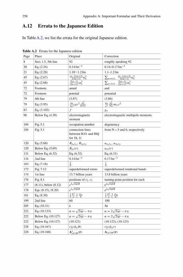
258 Appendix A: Important Formulae and Their Derivation
A.12 Errata to the Japanese Edition
In TableA.2, we list the errata for the original Japanese edition.
Table A.2 Errata for the Japanese edition
Page Place Original Correction
8 Sect. 1.5, 5th line 92 roughly speaking 92
20 Eq. (2.24) 0.14 fm−3 0.14–0.17 fm−3
21 Eq. (2.28) 1.18∼1.2 fm 1.1–1.2 fm
45 Eq. (2.67) (n−1)(n+2)2(2n+1) α2
n∑
n=4,5...(n−1)(n+2)2(2n+1) α2
n
45 Eq. (2.68) 5(n−1)(2n+1)2
α2n
∑n=4,5...
5(n−1)(2n+1)2
α2n
72 Footnote amnd and
72 Footnote potetial potential
79 4th line (3.87) (3.86)
79 Eq. (3.95) 4π3μ2 μc2 g2π
4π�c4πμ3
g2π3�c mπ c2
83 Eq. (3.103) f gπ
96 Below Eq. (4.38) electromagneticmoment
electromagnetic multipole moments
104 Fig. 5.1 occupation number degeneracy
104 Fig. 5.1 connection linesbetween H.O. and ISQfor 1h, 1i
from N=5 and 6, respectively
120 Eq. (5.68) Rnα�α , Rnβ �β unα�α , unβ �β
120 Below Eq. (5.69) Rn�(r) un�(r)
131 Below Eq. (6.32) Eq. (6.32) Eq. (6.31)
134 2nd line 0.14 fm−3 0.17 fm−3
163 Eq. (7.18) 29
19
172 Fig. 7.12 superdeformed rotors superdeformed rotational bands
174 1st line 13.7 billion years 13.8 billion years
176 Fig. 8.1 positions of r2, r3 turning point position for each
177 (8.11), below (8.12) e2√2ηk R e4
√2ηk R
178 Eqs. (8.15), (8.20) e2√2ηk R e4
√2ηk R
181 Eq. (8.30) 32
�2
μ1rc
pin�
32
�2
μ1rc
pin�2
199 2nd line 60 100
205 Eq. (10.31) k �k
222 Eq. (10.123) α = √2ηρ − πη α = 2
√2ηρ − πη
222 Below Eq. (10.127) α = √2ηρ − πη α = 2
√2ηρ − πη
222 Below Eq. (10.127) (10.123) (10.122), (10.123)
228 Eq. (10.167) r jI (kn R) r jI (knr)
228 Eq. (10.168) A∗λk I M (r) Aλk I M (r)
Appendix A: Important Formulae and Their Derivation 259
References
1. G.R. Satchler, Direct Nuclear Reactions (Clarendon Press, Oxford, 1983)2. K.W. Ford, J.A. Wheeler, Ann. Phys. 7:259 (1959); 287 (1959)3. W.E. Frahn, Ann. Phys. 72, 524 (1972); W.E. Frahn, M.S. Hussein, Nucl. Phys. A 346, 237
(1980)4. K.W. McVoy, Phys. Rev. C 3, 1104 (1971)5. N. Rowley, H.C. Doubre, C. Marty, Phys. Lett. B 69, 147 (1977)6. N. Takigawa, S.Y. Lee, Nucl. Phys. A 292, 173 (1977)7. M. Ueda, M.P. Pato, M.S. Hussein, N. Takigawa, Phys. Rev. Lett. 81, 1809 (1998)8. D.M. Brink, Semi-Classical Methods for Nucleus–Nucleus Scattering (Cambridge University
Press, London, 1985)9. D.M. Brink, N. Takigawa, Nucl. Phys. A 279, 159 (1977)10. S.Y. Lee, N. Takigawa, C. Marty, Nucl. Phys. A 308, 161 (1978)11. J.J. Sakurai, Modern Quantum Mechanics (Addison-Wesley, New York, 1985)12. W.E. Frahn, R.H. Lemmer, Nuovo Cimento 5, 1564 (1957); 6, 664 (1957); F.G. Perey, B. Buck,
Nucl. Phys. 32, 353 (1962)13. N. Takigawa, K. Hara, Z. Phys. A 276, 79 (1976)14. D.H.E. Gross, H. Kalinowski, Phys. Lett. B 48, 302 (1974); Phys. Rep. 45, 175 (1978)15. P. Fröbrich, R. Lipperheide, Theory of Nuclear Reactions (Clarendon Press, Oxford, 1996)16. H. Horiuchi, Prog. Theor. Phys. 63, 725 (1980); 64, 184 (1980)17. A. Messiah, Quantum Mechanics, vol. II (Elsevier, Amsterdam, 1962)18. D.M. Brink, G.R. Satchler, Angular Momentum (Oxford University Press, Oxford, 1962)19. A. Bohr, B.R. Mottelson, Nucl. Struct. vol. I (Benjamin, New York, 1969)20. P. Ring, P. Schuck, The Nuclear Many-Body problem (Springer, Berlin, 1980)21. DSc thesis of Yoshihiro Nozawa, Tohoku University (2002)22. M. Abramowitz, I.A. Stegun, Handbook of Mathematical Functions with Formulas, Graphs,
and Mathematical Tables (Dover, London, 1978)23. J.D. Jackson, Classical Electrodynamics, 3rd edn. (Wiley, New York, 1998)24. A. de-Shalit, I. Talmi, Nuclear Shell Theory (Academic, New York, 1963)
Index
Symbols1/v-law, 59, 218Δ(1232), 1, 3� particle, 3, 9Σ particle, 3, 9� particle, 9α particle, 15, 38α-decay, 191, 243α-nucleus, 33(α,p) reaction, 220α-particle model, 38, 179β-decay, 6, 45, 58, 219β-stability line, 22γ process, 220(γ, α) reaction, 220(γ ,n) reaction, 219(γ ,p) reaction, 220μ particle, 3ω-meson, 85, 88, 125π -meson, 3, 85
virtual, 1, 5ρ-meson, 3, 85, 87, 125σ -particle, 88, 125σωρ model, 1553H, 120, 122He, 2153He, 89, 120, 122, 1424He, 108Li, 2156Li, 336,7Li, 238,9Li, 2311Li, 22, 238Be, 33, 63, 173, 179, 187, 19710B, 3312C, 33, 38, 173, 18013C, 120
14C, 71, 191, 20014N, 33, 71, 11915N, 25, 7114O, 7115O, 25, 7116O, 1, 33, 38, 108, 117, 17320Ne, 17324Mg, 38, 17348Ca, 13045Sc, 2, 11956Fe, 40, 21562Ni, 33, 40, 215Ge, 17390Sr, 60Tc, 33Cd, 209112Cd, 172105Te, 220137Cs, 60150Ce, 44Pm, 33150Sm, 44166Er, 171167Er, 171, 182180Ta, 33189Os, 120Au, 15, 20Hg, 173, 180182Hg, 173184Hg, 173, 185186Hg, 173208Hg, 44206Pb, 191208Pb, 22, 44, 117209Pb, 117210Pb, 127, 164, 168, 171209Bi, 33, 118, 119
© Springer Japan 2017N. Takigawa and K. Washiyama, Fundamentals of Nuclear Physics,DOI 10.1007/978-4-431-55378-6
261
262 Index
210Po, 15, 122, 127, 171, 191, 196, 197, 245Rn, 208226Ra, 201230Th, 61231Th, 61U, 208, 215235U, 46, 49, 55, 57, 58236U, 55238U, 49, 55, 57, 63, 211239U, 54, 55237Np, 60, 192239Pu, 46240Pu, 63Cm, 130Cf, 130258Fm, 201Nh (Nihonium), 131Fl (Flerovium), 132Mc (Moscovium), 132Lv (Livermorium), 132Ts (Tennessine), 132Og (Oganesson), 132
AAbsorber, 16Abundance of elements, 9Actinides, 173, 187Action integral, 230Airy function, 231Alkali metals, 117Allowed states, 197Alvarez, L., 36Anomalous magnetic moments, 4, 5, 99,
122, 123Argonne potential, 88Arima, A., 122Arrhenius factor, 201Astrophysical S-factor, 216Asymmetric fission, 46, 108Atomic model, 15Atomic number, 1Attenuation method, 26
BBarrier transmission probability, 231Bartlett operator, 70Baryons, 1BCS, 164Bernoulli’s formula, 149Bethe–Goldstone equation, 93Big Bang nucleosynthesis, 215Bimodal fission, 201
Binding energy, 32, 110BNL, 11Bohr magneton, 4Bohr radius, 30Bohr, N., 46, 117Boltzmann constant, 217Bonn potential, 88Born approximation, 19, 82, 233Breathing mode of vibration, 146Brink–Boeker force, 95Broken spatial symmetry, 39Brownian motion, 202Brueckner theory, 93
CCapture reaction, 218Caustics, 225Central potential, 72CERN, 11Chain reaction, 57, 58Channel-coupling effects, 235Channel radius, 198Charge distribution, 22Charge-exchange operator, 70Charge independence, 71, 80
breaking, 88Charge symmetry, 71
breaking, 89Chiral perturbation theory, 88Classical liquid, 23, 212Classical optics, 16Classical orbits, 14Classical trajectories, 15Classical turning points, 54Clebsch–Gordan coefficient, 105, 127Closed form expression, 224Cluster decay, 191Clusterization, 199Cluster model, 38, 179, 197Cluster structure, 38, 95, 126CNO cycle, 34Coester line, 156Coherence length, 169Cold fusion, 130Collective model, 98Collective motion, 212Commutation relation, 30Comparison equation, 229Complete fusion reaction, 202Complex scaling method, 192Compound nucleus reactions, 107, 117Compton wavelength, 66, 87
Index 263
Configuration mixing, 120, 121Constant Δ method, 185Constant G method, 185Constrained Hartree–Fock, 184Control rod, 58Convection current, 99Core polarization, 120, 121, 207Correlation length, 169Coulomb barrier, 7Coulomb energy, 42Coulomb excitation, 211Coulomb gauge, 248Coulomb scattering, 14Coulomb trajectory, 17Coulomb wave functions, 245Critical mass, 58Critical temperature, 200Cumulant expansion method, 27
DD’Alembert equation, 66Daughter nucleus, 48De Broglie wavelength, 17Debye–Hückel formula, 31Decay channel, 38Decay width, 38, 192Deep inelastic collision (DIC), 202Deep potential, 197Deformation
oblate, 106prolate, 106
Deformation parameter, 106, 174αλ, 49αλμ, 49, 174β, γ , 176δ, 174
Deformed shell model, 177Degeneracy pressure, 29, 41Degree of non-locality, 236Delayed neutrons, 58Density distribution, 20Density of nuclear matter, 22Deuterium, 32Deuteron, 1, 8, 32, 74, 76, 215Diffraction, 16Diffraction effect, 17Diffraction pattern, 20Diffractive eikonal approximation, 27Dirac equation, 4, 99Dissipation, 202Distance of closest approach, 15Distortion effects, 21
Double folding potential, 233Doubly-closed shell nucleus, 117Doubly-magic ±2 nuclei, 164Doubly-magic nucleus, 117D quark, 9, 123Dtμ molecule, 37D3h symmetry, 38
EE4/E2 ratio, 173Effective charge, 207Effective many-body interaction, 141Effective mass, 57, 136, 138, 139, 144, 147,
154, 234, 235e-mass, 148, 155k-mass, 155ω-mass, 155
Effective range, 79, 80Effective range theory, 78, 79Effective sharp radius, 23Eikonal approximation, 27, 232Electric charge distribution, 4Electric dipole moment, 98Electric multipole operator, 102Electric multipole radiation, 251Electric quadrupole moment, 98, 105, 171,
211Electric transition, 205Electromagnetic field, 97Electromagnetic force, 17Electromagnetic interaction, 6Electromagnetic moments, 97Electromagnetic transitions, 191, 209, 246Electron, 3Electron capture, 29, 41, 45Elliott’s SU (3) model, 39Energy density, 145Energy dependent potential, 235Energy problem, 36Enriched uranium, 58, 59Equation of state, 141, 147, 148Equilateral triangle configuration, 38Equivalent local potential, 136, 139, 234,
237Equivalent radius, 23Escape path method, 201Euler angles, 175, 243Euler–Lagrange equation, 86, 157Evaporation theory, 59Even–odd property, 33Exchange force, 81Exchange operator, 68Exchange potentials, 234
264 Index
FFaddeev equation, 142Fast reactor (fast neutron reactor), 59Fermi, E., 58Fermi energy, 29, 94, 110, 167Fermi-gas model, 28Fermi momentum, 28Fermi’s golden rule, 203Fermi velocity, 29Feshbach, H., 94Fissility parameter, 49–51Fission, 41, 46, 57, 107, 117, 200
decay width, 56energy release, 47half-life, 55threshold energy, 55
Fission barrier, 48, 54, 62Fission coordinate, 49Fission isomer, 60, 62, 63, 187Fission lifetime, 201Fock potential, 234Fokker–Planck equation, 202Form factor, 20, 24Fourier transformation, 67Fragmentation reactions, 147, 152Fraunhofer diffraction, 20, 26Fraunhofer scattering, 25Fresnel diffraction, 16Fresnel scattering, 16Friction, 202Fusion reactions, 33, 41
GGamow energy, 217Gamow factor, 195, 199, 200Gamow model, 193, 198, 243Gamow peak, 216, 217Gap equation, 167Gap parameter, 167, 186Gaussian type, 23Geiger, H., 13Geiger–Nuttal rule, 200Geometrical collective model, 175, 209g-factor, 99, 122, 247Giant quadrupole resonance (GQR), 212Giant resonances, 17Glauber theory, 27, 232Glory scattering, 225G-matrix, 92Gogny force, 96Gradient formulae, 251Gravitational collapse, 41
Gravitational force, 6Green function, 67
HHadrons, 1Hahn, O., 46Half-life, 6Halo nucleus, 23Hamada–Johnston potential, 88, 89Hard core, 41, 93Hard-core potential, 88Harmonic oscillator, 111Hartree–Fock–Bogoliubov (HFB), 164Hartree–Fock calculations, 96Hartree potential, 140Hasegawa–Nagata force, 95Heavy-ion fusion reactions, 171, 211Heavy particle decay, 191, 200Heisenberg operator, 70Heisenberg valley, 43–45Hikosaka, Tadayoshi, 116Hofstadter, R., 17Horie, H., 122Hot fusion, 130Hoyle-state, 38Hulthén, L., 77Hybrid model, 39Hyperdeformed states, 62Hyperfine structure, 100Hypernuclei, 9, 17Hyperons, 151
IIkeda diagram, 38Incoming wave boundary condition, 218Incompressibility, 142, 145Independent particle model, 116Induced fission, 46, 47, 202Inelastic scattering, 15Inertial confinement, 36Infinite square-well potential, 110Integral representation, 224Integro-differential equation, 234Interacting boson model (IBM), 175Interference, 225Internal conversion, 211Internal conversion coefficient, 211Intrinsic electric quadrupole moment, 105Intrinsic energy dependence, 235Intrinsic quadrupole moment, 211, 242Intruder states, 116
Index 265
Irreducible tensor, 239Irrotational incompressible fluid, 210Isobaric multiplet, 71Isobars, 8Isoscalar monopole vibration, 146Isospin, 2, 3Isospin-exchange operator, 70Isospin operators, 2Isospin singlet, 43Isospin space, 2Isospin triplet, 43Isotones, 8Isotopes, 8Isotope variation of the charge radii, 186
JJahn–Teller effect, 40, 179Jensen, J.H.D., 117J-PARC, 9
KKinetic energy density, 144Klein–Gordon equation, 66K quantum number, 40Kramers factor, 202Kramers formula, 202
LLadder scattering, 93Landé formula, 242Lane potential, 125Langer replacement, 226Langevin equation, 202Lattice QCD, 88Level density parameter, 155LHC, 11Linear accelerator, 17Liquid-drop model, 28, 42, 47, 107, 117,
210, 212Liquid–gas phase transition, 152Local density approximation, 137Local momentum approximation, 235, 237Long wave length approximation, 204
MMacroscopic–microscopic method, 57, 182,
201Magic numbers, 9, 74, 107, 108, 112, 116,
117, 219atom, 108, 117
microcluster, 117Magnetic charge distribution, 4Magnetic confinement, 36Magnetic dipole moment, 3, 98, 105Magnetic effects, 24Magnetic moment, 4, 75, 97, 119, 247Magnetic multipole operator, 102Magnetic multipole radiation, 251Magnetic radiation, 203Magnetic transition, 205Magnetization current, 99Magneton, 3Main sequence stars, 33Majorana exchange term, 95Majorana force, 82Majorana operator, 70Marsden, E., 13Mass density, 29Mass distribution, 26Mass formula, 42Massive star, 40Mass number, 1Maxwell–Boltzmann distribution, 217Mayer, M.G., 117Mean field, 109Mean life, 3Mean square charge radius, 3Mean-square radius, 23Mechanical instability, 153Meitner, Lise, 46Meson effect, 122Meson exchange current, 100Meson theory, 5, 65, 85Metal microclusters, 40Method of steepest descent, 217, 224Minnesota force, 95Mirror nuclei, 25, 71Molecular dynamics calculations, 38Molecular point of view, 38Molecular structure, 38Moment of inertia, 212Mott scattering, 20Multiple scattering, 93Multipole moments, 171Multipole transition operator, 204Muon-catalysed fusion (μCF), 36Muonic-atom, 25
NNagaoka, Hantaro, 13Natural radioactive nucleus, 15Neutrino, 34, 220
266 Index
Neutrino oscillation, 36Neutron, 1, 2Neutron absorber, 57, 58Neutron capture, 215, 218, 219Neutron-deficient nuclei, 108, 220Neutron distribution, 22Neutron drip line, 22, 23Neutron flux, 219Neutron halo, 22, 23Neutron-induced fission, 46Neutron moderator, 57, 58Neutron number, 2Neutron-rich nuclei, 219Neutron-rich unstable nuclei, 108Neutron skin, 22Neutron star, 6, 146, 151, 163, 220(n,γ ) reaction, 219Nijmegen potential, 88Nilsson levels, 180Nix, J.R., 49Noble gases, 107, 108Nolen–Schiffer anomaly, 89Noncentral potential, 73Non-locality, 235Non-local potential, 136, 234Nuclear chart, 8, 9, 73, 173, 187Nuclear energy, 57Nuclear force, 7, 41, 65
charge dependence, 89density dependence, 94exchange property, 95mesons, 91radial form factor, 95range, 65state dependence, 80, 92
Nuclear interaction, 17Nuclear magneton, 4Nuclear matter, 11, 137Nuclear potential, 109Nuclear power, 57Nuclear radius, 20Nuclear reaction in matter, 38Nuclear waste, 60Nucleon, 2Nucleon–nucleon scattering, 74, 78Nucleon–nucleus reaction, 27Nucleosynthesis, 42Nucleus, 1, 13Nucleus–nucleus reaction, 27Number density, 28
OOctupole vibration, 175
Odd–even mass parameter, 33Odd–odd nuclei, 33Oklo, 60One-pion exchange potential (OPEP), 87, 92Onion layer structure, 40Optical limit, 232Optical limit formulae, 27Optical potential, 229Optical theorem, 224, 233Oscillator parameter, 112Overlap function, 27
PPairing
monopole, 163, 165multipole, 163quadrupole, 163
Pairing correlation, 33, 42, 55, 58, 127, 128,130, 162
Pairing energy, 254Parahydrogen molecule, 79Paris potential, 88Partial wave expansion, 223Particle–vibration coupling, 155Pauli exclusion principle, 29, 93, 109, 179,
197Pauli forbidden states, 197, 244Pauli, W.E., 4Penetration factor, 198Perfect rigid sphere model, 141Periodic table of the elements, 107, 108, 117(p,γ ) reaction, 220Phase diagram of nuclear matter, 11Phase shift, 79, 83Phase shift analysis, 78Photo-disintegration, 41, 220Plum pudding model, 13Point group, 38Poisson equation, 19, 30Poisson sum formula, 26, 225Polarization, 85, 235Polarized electrons, 4, 22Polarized projectile, 78Polarized protons, 22Polarized target, 78Pole of the S-matrix, 192Polyatomic molecule, 40Pp collision in the Sun, 7Pp-chain (proton–proton chain) reactions,
34PpI-chain reactions, 34PpII-chain reactions, 34
Index 267
PpIII-chain reactions, 34P-process, 220Preformation factor, 199Pressure, 145, 149Presupernova star, 40Primordial nucleosynthesis, 215Projection operator, 68, 70Projection operator method, 94Projection theorem, 76, 120, 241Prompt neutrons, 58Proton, 1, 2Proton decay, 197Proton distribution, 22Proton–nucleus scattering, 26Proton radioactivity, 191Proton-rich nuclei, 108
QQCD phase diagram, 11Quadrupole moment, 76, 242Quadrupole vibration, 175Quantization condition, 194, 245Quantum chromodynamics (QCD), 1, 65, 85Quantum decay, 200Quantum fluctuation, 202Quantum liquid, 23, 212Quantum mechanics, 1Quantum tunneling, 8, 48, 200Quark cluster model, 88Quark–gluon plasma, 11Quark model, 3, 5, 123Quarks, 1Quasi-fission, 202Quasi-spin formalism, 130, 164Quenching effect, 100, 122Q-value, 47
RRadiation gauge, 248Radiative neutron capture, 97Radioactivity, 191Radius parameter, 23Rainbow scattering, 225Raisin bread model, 13Random walk, 202Rapid neutron capture, 41Rare-earth, 169, 187, 208Reactivation probability, 37Reactor, 54, 57, 59Recoupling coefficient, 254Red giant stars, 215
Reduced matrix element, 241Reduced transition probability, 203, 205Reduced width, 199Redundant states, 197, 244Refraction effect, 17Reid potential, 88, 91Relativistic effects, 20Relativistic mean-field theory, 29, 125, 155Reorientation effect, 211Repulsive core, 83, 88, 92, 197Residual interaction, 121, 128, 254Resonance, 115Resonating group method (RGM), 197, 234Respiration, 108Rest energy, 18RHIC, 11R-matrix, 115, 198Root-mean-square radius, 23Rosenfeld force, 95Rotation, 238Rotational band, 38, 63, 173Rp-process, 220R-process, 41, 42, 215, 219Rutherford, E., 13Rutherford model for atom, 14Rutherford scattering, 13, 14
SSaddle point, 51Saturation property, 95, 140, 148
binding energy, 33, 107density, 23, 28, 107
Saturn model, 13Scalar product, 242Scattering length, 79, 80Schmidt lines, 120Schrödinger equation, 18Scission point, 46Screened Coulomb potential, 30Screening effect, 30, 36, 217Screening energy, 216Screening length, 31Segré chart, 8Segré, E., 14Selection rules, 58, 104, 205Self-consistency condition, 177Semi-classical theory, 26, 193, 227Semi-Empirical mass formula, 42Seniority, 164Separable type, 236Separation energy, 32Serber force, 82, 95, 126, 140
268 Index
Shadow scattering, 25, 26Shallow potential, 197Shape coexistence, 173Shape transition, 173Sharp-cut-off-model, 26Shell correction, 49Shell correction energy, 131Shell effect, 8, 48Shell model, 22, 38, 98, 116Shell structure, 107, 179SHIP, 131Si-burning reaction, 40Single particle model, 119Single-Particle model estimate, 206Skyrme force, 96, 141Skyrme, T.H.R., 141Soft-core potential, 88Solar neutrino problem, 36Sommerfeld parameter, 194, 216Sommerfeld–Watson transformation, 224,
225Space-exchange operator, 70Spherical spinors, 159Spin of photon, 249Spin-exchange operator, 69, 70Spin-flip, 85Spinodal line, 148, 152, 154Spin–orbit coupling, 160Spin–orbit density, 144Spin–orbit interaction, 39, 73, 114, 116, 125,
142Spontaneous fission, 46, 47, 201S-process, 45, 215, 219S quark, 9Stability line, 43, 219Stationary phase approximation, 224Stellar nucleosynthesis, 215Stern, O., 4, 97, 100Sticking probability, 37Stopping power, 36Strangeness, 3Strassmann, F., 46Strong absorption, 17Strong interaction, 1, 6, 65Structure of nucleon, 17Strutinsky method, 182Superdeformed states, 62, 187Superfluidity, 186
1S0, 1633P2, 163
Superheavy elements, 8, 42, 130Superheavy nuclei, 8
Supernova explosion, 29, 41, 146, 151, 215,219
Surface diffuseness parameter, 22Surface effect, 42, 116Surface energy, 54Surface tension, 42Surface term, 42Surface thickness, 148, 154Symmetry, 38, 65Symmetry energy, 42Synthesis of elements, 6, 97, 215
TTani–Foldy–Wouthuysen transformation,
160Teichmann–Wigner sum rule, 199Tensor force, 73, 75, 87, 92, 116, 125, 126Tensor operator, 73, 237Thermal decay, 200, 202Thermal fission, 202Thermal hopping, 200Thermal neutron, 55, 79Thermal nuclear reactions, 215Thomas–Fermi approximation, 28, 31, 43,
144extended, 152
Thompson, J.J., 13Thompson model, 14Three-body force, 142Threshold energy, 115Time-reversal operator, 165T -matrix, 93Transition state theory, 202Translation, 238Transmutation, 60Transparency function, 27Transverse gauge, 248Triaxial, 176Tritium, 3, 32Triton, 32, 89, 142Tunneling probability, 194, 246Turning points, 54, 229Two-Potential approach, 195
UUniform approximation, 53, 231Unitarity condition, 224Unitary model operator approach (UMOA),
94Unstable nuclei, 22, 42, 108, 219U quark, 9, 123
Index 269
Vvan der Waals equation of state, 152Variational method, 95Vector function, 248Vector spherical harmonics, 250Vector wave function, 248Vesman mechanism, 37Viscosity, 202Volkov interaction, 95, 126Volume term, 42
WWaiting point nuclei, 219Waiting points, 219Weak interaction, 6, 8Weisskopf units, 207Weizsäcker–Bethe mass formula, 42Weizsäcker correction, 152
Well-behaved potential, 140Wheeler, J.A., 46Whittaker functions, 231Wiener process, 202Wigner D function, 210Wigner–Eckart theorem, 104, 241Wigner force, 82Wigner limit, 199Wigner transformation, 236Wildermuth condition, 197WKB approximation, 137, 194, 227Woods–Saxon, 22Woods–Saxon potential, 110, 114
YYamanouchi, Takahiko, 116Yukawa function, 87