Embed Size (px)
Citation preview
1 - 1Fundamentals of Kalman Filtering:A Practical Approach
Fundamentals of Kalman Filtering:A Practical Approach
Paul Zarchan
1 - 2Fundamentals of Kalman Filtering:A Practical Approach
Seminar Outline - 1
• Numerical Techniques- Required background- Introduction to source code
• Method of Least Squares- How to build batch process least squares filter- Performance and software comparison of different order filters
• Recursive Least Squares Filtering- How to make batch process filter recursive- Formulas and properties of various order filters
1 - 3Fundamentals of Kalman Filtering:A Practical Approach
Seminar Outline - 2
• Polynomial Kalman Filters- Relationship to recursive least squares filter- How to apply Kalman filtering and Riccati equations- Examples of utility in absence of a priori information
• Kalman Filters in a Non Polynomial World- How polynomial filter performs when mismatched to real world- Improving Kalman filter with a priori information
• Continuous Polynomial Kalman Filter- How continuous filters can be used to understand discrete filters- Using transfer functions to represent and understand Kalman filters
1 - 4Fundamentals of Kalman Filtering:A Practical Approach
Seminar Outline - 3
• Extended Kalman Filtering- How to apply equations to a practical example- Showing what can go wrong with several different design approaches
• Drag and Falling Object- Designing two different extended filters for this problem- Demonstrating the importance of process noise
• Cannon Launched Projectile Tracking Problem- Comparing Cartesian and polar extended filters in terms of performance and software requirements- Comparing extended and linear Kalman filters in terms of performance and robustness
1 - 5Fundamentals of Kalman Filtering:A Practical Approach
Seminar Outline - 4
• Tracking a Since Wave- Developing different filter formulations and comparing results
• Satellite Navigation (Simplified GPS Example)- Step by step approach for determining receiver location based on satellite range measurements
• Biases- Filtering techniques for estimating biases in GPS example
• Linearized Kalman Filtering- Two examples and comparisons with extended filter
• Miscellaneous Topics- Detecting filter divergence- Practical illustration of inertial aiding
1 - 6Fundamentals of Kalman Filtering:A Practical Approach
Seminar Outline - 5
• Tracking an Exoatmospheric Target- Comparison of Kalman and Fading Memory Filters
• Miscellaneous Topics 2 - Using additional measurements - Batch processing - Making filters adaptive
• Filter Banks• Practical Uses of Chain Rule
- 3D GPS• Finite Memory Filter• Extra
- Stereo, Filtering Options, Cramer-Rao & More
1 - 7Fundamentals of Kalman Filtering:A Practical Approach
Numerical Basics
1 - 8Fundamentals of Kalman Filtering:A Practical Approach
Numerical BasicsOverview
• Simple vector and matrix operations• Numerical integration• Noise and random variables
- Definitions- Gaussian noise example- Simulating white noise
• State space notation• Fundamental matrix
1 - 9Fundamentals of Kalman Filtering:A Practical Approach
Simple Vector and Matrix Operations
1 - 10Fundamentals of Kalman Filtering:A Practical Approach
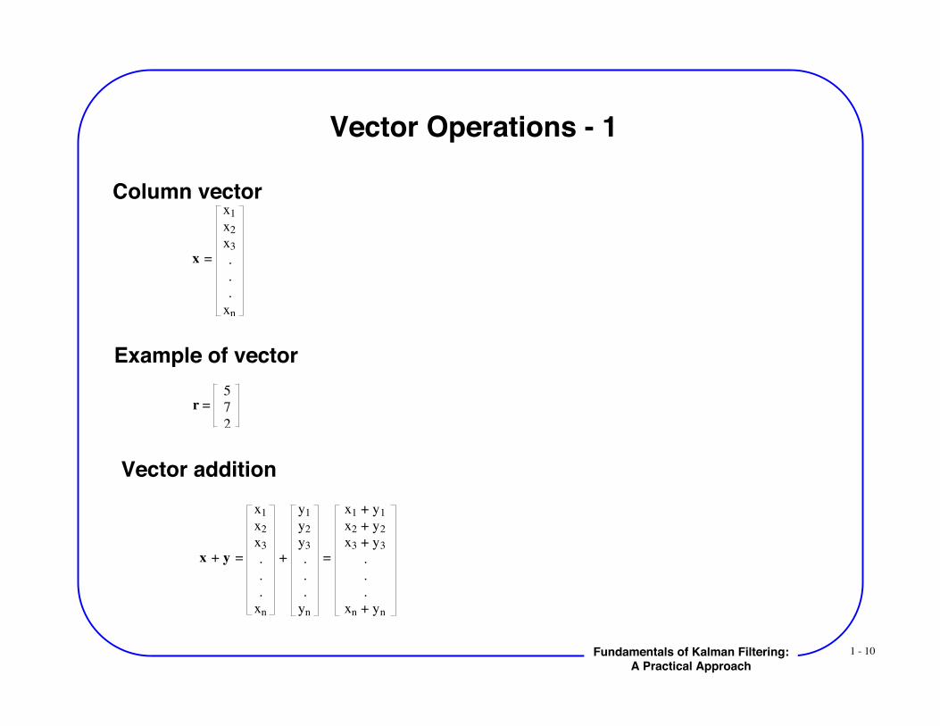
Vector Operations - 1
Column vector
x =
x1
x2
x3
.
.
.
xn
Example of vector
r =
5
7
2
Vector addition
x + y =
x1
x2
x3
.
.
.
xn
+
y1
y2
y3
.
.
.
yn
=
x1 + y1
x2 + y2
x3 + y3
.
.
.
xn + yn
1 - 11Fundamentals of Kalman Filtering:A Practical Approach
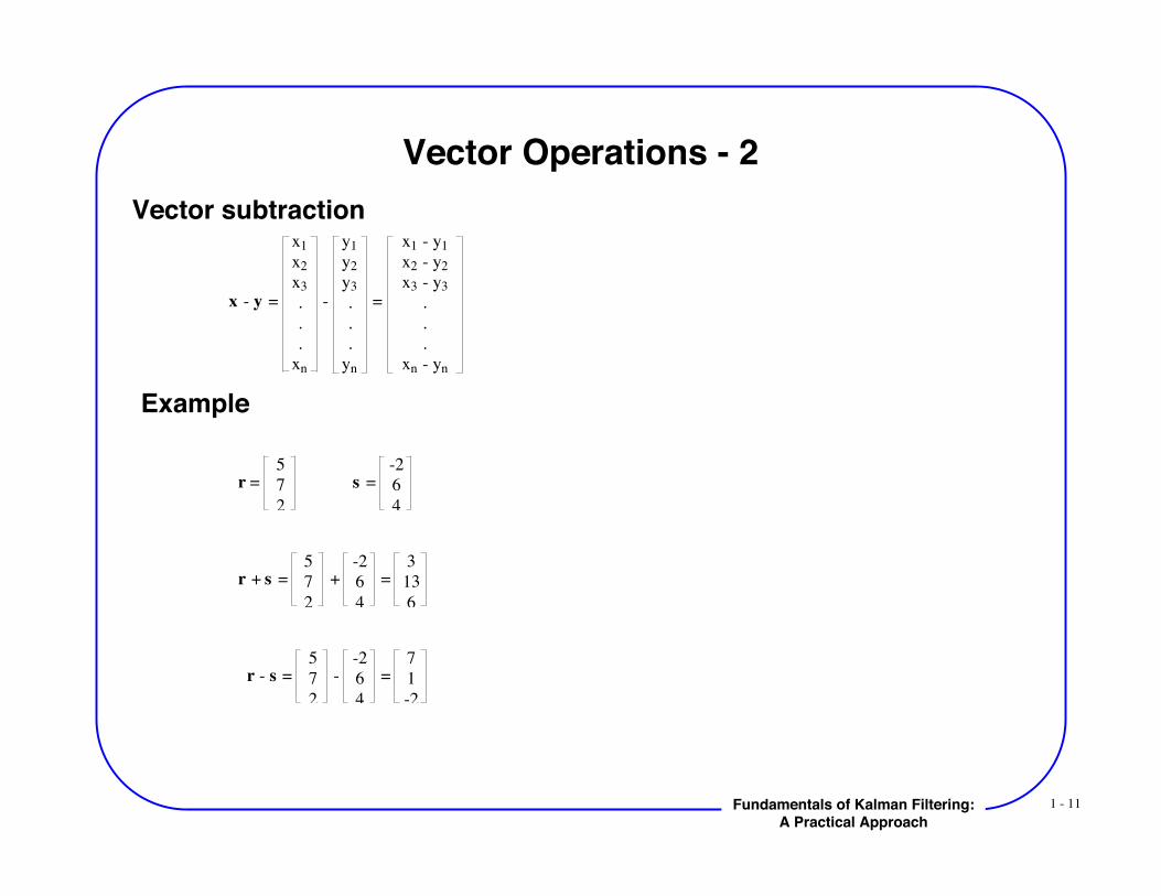
Vector Operations - 2Vector subtraction
x - y =
x1
x2
x3
.
.
.
xn
-
y1
y2
y3
.
.
.
yn
=
x1 - y1
x2 - y2
x3 - y3
.
.
.
xn - yn
Example
s =
-2
6
4
r =
5
7
2
r + s =
5
7
2
+
-2
6
4
=
3
13
6
r - s =
5
7
2
-
-2
6
4
=
7
1
-2
1 - 12Fundamentals of Kalman Filtering:A Practical Approach
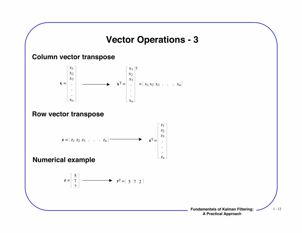
Vector Operations - 3Column vector transpose
x =
x1
x2
x3
.
.
.
xn
xT =
x1
x2
x3
.
.
.
xn
T
= x1 x2 x3 . . . xn
Row vector transpose
z = z1 z2 z3 . . . zn zT =
z1
z2
z3
.
.
.
znNumerical example
r =
5
7
2
rT = 5 7 2
1 - 13Fundamentals of Kalman Filtering:A Practical Approach
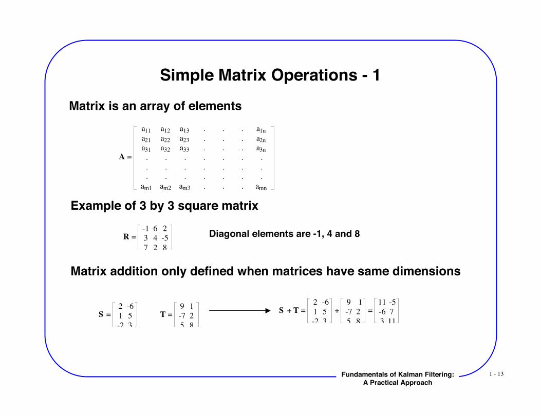
Simple Matrix Operations - 1Matrix is an array of elements
A =
a11 a12 a13 . . . a1n
a21 a22 a23 . . . a2n
a31 a32 a33 . . . a3n
. . . . . . .
. . . . . . .
. . . . . . .
am1 am2 am3 . . . amn
Example of 3 by 3 square matrix
R =
-1 6 2
3 4 -5
7 2 8
Diagonal elements are -1, 4 and 8
Matrix addition only defined when matrices have same dimensions
S =
2 -6
1 5
-2 3
T =
9 1
-7 2
5 8
S + T =
2 -6
1 5
-2 3
+
9 1
-7 2
5 8
=
11 -5
-6 7
3 11
1 - 14Fundamentals of Kalman Filtering:A Practical Approach
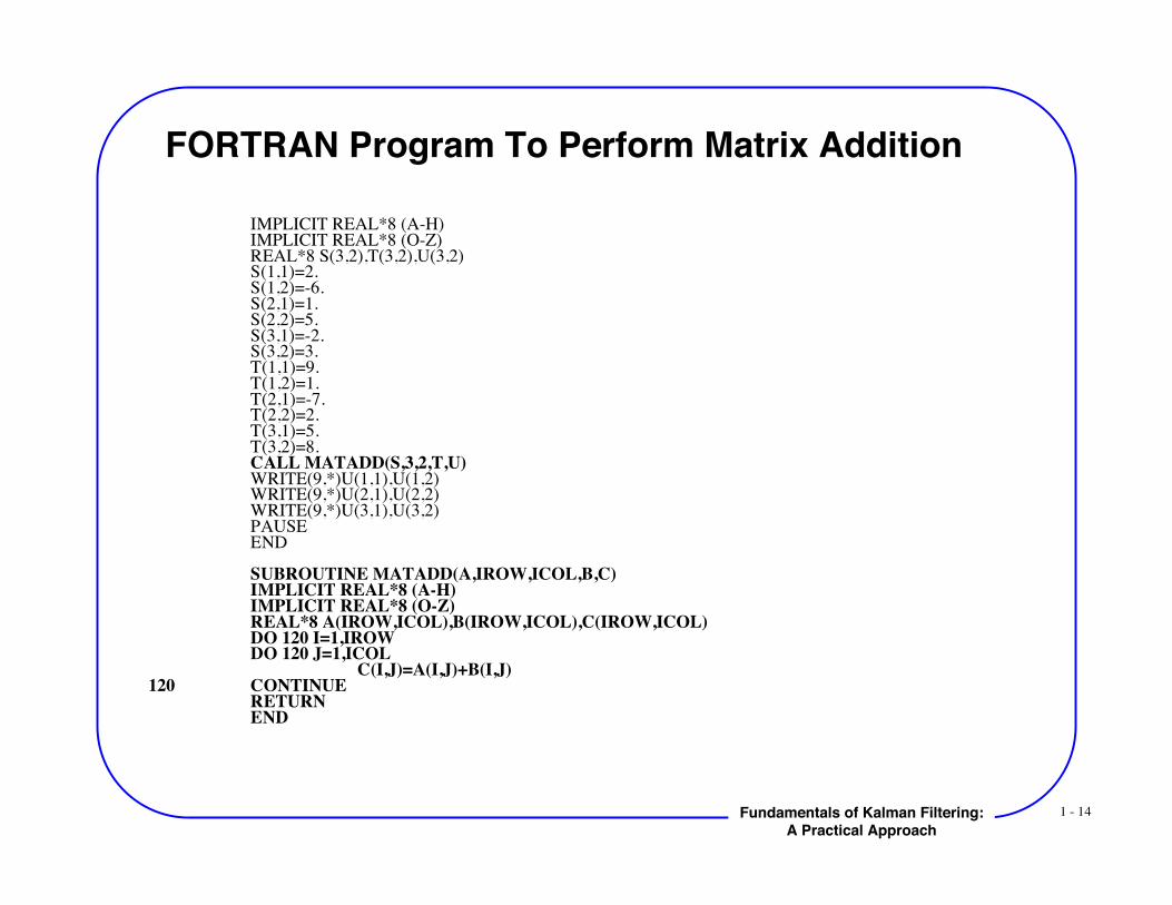
FORTRAN Program To Perform Matrix Addition
IMPLICIT REAL*8 (A-H)IMPLICIT REAL*8 (O-Z)REAL*8 S(3,2),T(3,2),U(3,2)S(1,1)=2.S(1,2)=-6.S(2,1)=1.S(2,2)=5.S(3,1)=-2.S(3,2)=3.T(1,1)=9.T(1,2)=1.T(2,1)=-7.T(2,2)=2.T(3,1)=5.T(3,2)=8.
CALL MATADD(S,3,2,T,U) WRITE(9,*)U(1,1),U(1,2)
WRITE(9,*)U(2,1),U(2,2)WRITE(9,*)U(3,1),U(3,2)
PAUSEEND
SUBROUTINE MATADD(A,IROW,ICOL,B,C)IMPLICIT REAL*8 (A-H)IMPLICIT REAL*8 (O-Z)REAL*8 A(IROW,ICOL),B(IROW,ICOL),C(IROW,ICOL)
DO 120 I=1,IROWDO 120 J=1,ICOL
C(I,J)=A(I,J)+B(I,J) 120 CONTINUE RETURN
END
1 - 15Fundamentals of Kalman Filtering:A Practical Approach
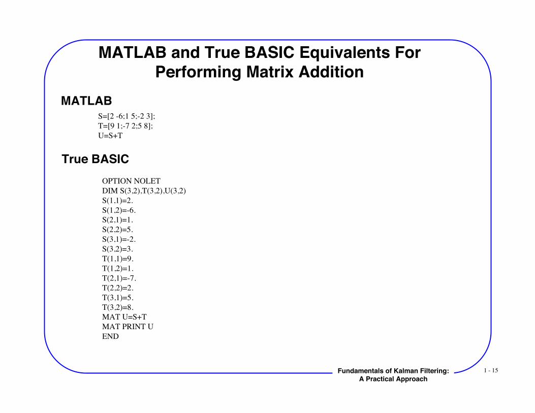
MATLAB and True BASIC Equivalents ForPerforming Matrix Addition
S=[2 -6;1 5;-2 3];T=[9 1;-7 2;5 8];U=S+T
OPTION NOLETDIM S(3,2),T(3,2),U(3,2)S(1,1)=2.S(1,2)=-6.S(2,1)=1.S(2,2)=5.S(3,1)=-2.S(3,2)=3.T(1,1)=9.T(1,2)=1.T(2,1)=-7.T(2,2)=2.T(3,1)=5.T(3,2)=8.MAT U=S+TMAT PRINT UEND
MATLAB
True BASIC
1 - 16Fundamentals of Kalman Filtering:A Practical Approach
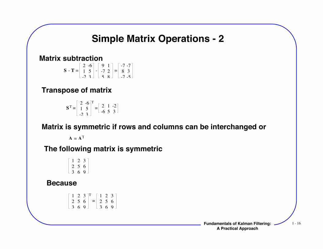
Simple Matrix Operations - 2
S - T =
2 -6
1 5
-2 3
-
9 1
-7 2
5 8
=
-7 -7
8 3
-7 -5
Matrix subtraction
Transpose of matrix
ST =
2 -6
1 5
-2 3
T
= 2 1 -2
-6 5 3
Matrix is symmetric if rows and columns can be interchanged orA = AT
The following matrix is symmetric1 2 3
2 5 6
3 6 9
Because1 2 3
2 5 6
3 6 9
T
=
1 2 3
2 5 6
3 6 9
1 - 17Fundamentals of Kalman Filtering:A Practical Approach
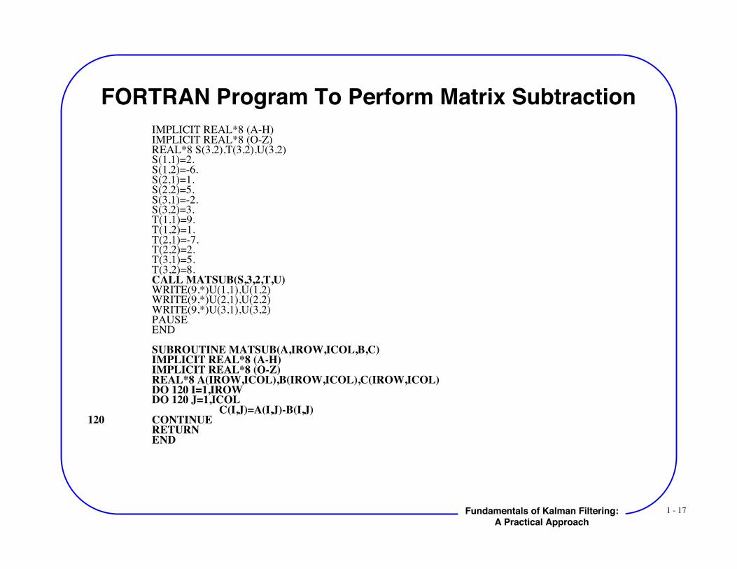
FORTRAN Program To Perform Matrix SubtractionIMPLICIT REAL*8 (A-H)IMPLICIT REAL*8 (O-Z)REAL*8 S(3,2),T(3,2),U(3,2)S(1,1)=2.S(1,2)=-6.S(2,1)=1.S(2,2)=5.S(3,1)=-2.S(3,2)=3.T(1,1)=9.T(1,2)=1.T(2,1)=-7.T(2,2)=2.T(3,1)=5.T(3,2)=8.
CALL MATSUB(S,3,2,T,U) WRITE(9,*)U(1,1),U(1,2)
WRITE(9,*)U(2,1),U(2,2)WRITE(9,*)U(3,1),U(3,2)
PAUSEEND
SUBROUTINE MATSUB(A,IROW,ICOL,B,C)IMPLICIT REAL*8 (A-H)IMPLICIT REAL*8 (O-Z)REAL*8 A(IROW,ICOL),B(IROW,ICOL),C(IROW,ICOL)
DO 120 I=1,IROWDO 120 J=1,ICOL
C(I,J)=A(I,J)-B(I,J) 120 CONTINUE RETURN
END
1 - 18Fundamentals of Kalman Filtering:A Practical Approach
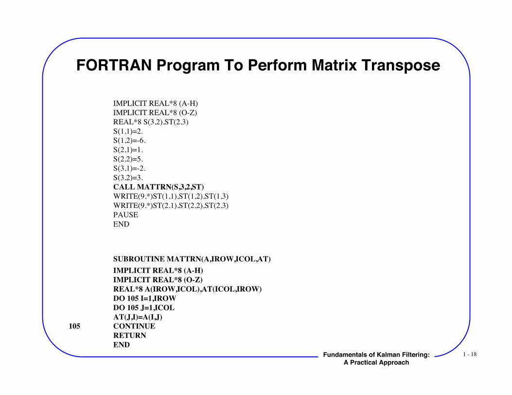
FORTRAN Program To Perform Matrix Transpose
IMPLICIT REAL*8 (A-H)IMPLICIT REAL*8 (O-Z)REAL*8 S(3,2),ST(2,3)S(1,1)=2.S(1,2)=-6.S(2,1)=1.S(2,2)=5.S(3,1)=-2.S(3,2)=3.
CALL MATTRN(S,3,2,ST) WRITE(9,*)ST(1,1),ST(1,2),ST(1,3)
WRITE(9,*)ST(2,1),ST(2,2),ST(2,3) PAUSE
END
SUBROUTINE MATTRN(A,IROW,ICOL,AT)IMPLICIT REAL*8 (A-H)IMPLICIT REAL*8 (O-Z)REAL*8 A(IROW,ICOL),AT(ICOL,IROW)DO 105 I=1,IROWDO 105 J=1,ICOLAT(J,I)=A(I,J)
105 CONTINUE RETURN
END
1 - 19Fundamentals of Kalman Filtering:A Practical Approach
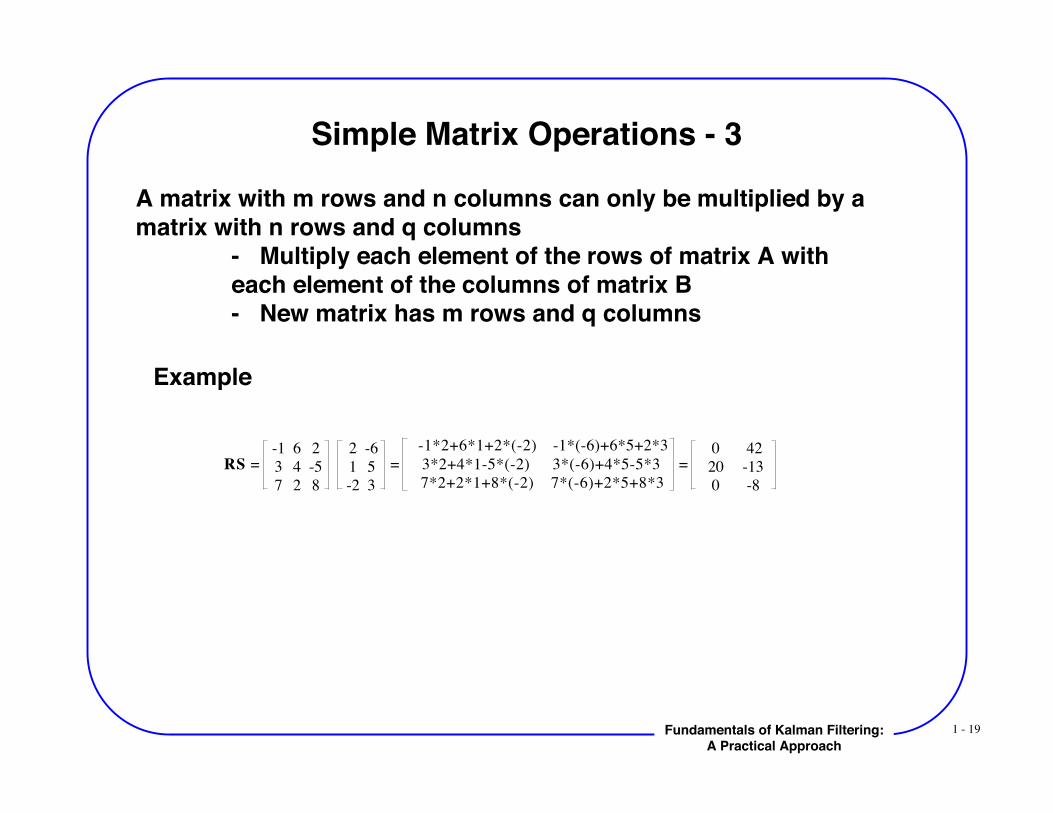
Simple Matrix Operations - 3
A matrix with m rows and n columns can only be multiplied by amatrix with n rows and q columns
- Multiply each element of the rows of matrix A with each element of the columns of matrix B- New matrix has m rows and q columns
Example
RS = -1 6 2
3 4 -5
7 2 8
2 -6
1 5
-2 3
=
-1*2+6*1+2*(-2) -1*(-6)+6*5+2*3
3*2+4*1-5*(-2) 3*(-6)+4*5-5*3
7*2+2*1+8*(-2) 7*(-6)+2*5+8*3
= 0 42
20 -13
0 -8
1 - 20Fundamentals of Kalman Filtering:A Practical Approach
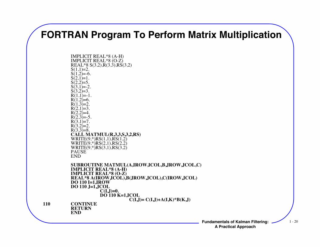
FORTRAN Program To Perform Matrix Multiplication
IMPLICIT REAL*8 (A-H)IMPLICIT REAL*8 (O-Z)REAL*8 S(3,2),R(3,3),RS(3,2)S(1,1)=2.S(1,2)=-6.S(2,1)=1.S(2,2)=5.S(3,1)=-2.S(3,2)=3.R(1,1)=-1.R(1,2)=6.R(1,3)=2.R(2,1)=3.R(2,2)=4.R(2,3)=-5.R(3,1)=7.R(3,2)=2.R(3,3)=8.
CALL MATMUL(R,3,3,S,3,2,RS) WRITE(9,*)RS(1,1),RS(1,2)
WRITE(9,*)RS(2,1),RS(2,2)WRITE(9,*)RS(3,1),RS(3,2)
PAUSEEND
SUBROUTINE MATMUL(A,IROW,ICOL,B,JROW,JCOL,C)IMPLICIT REAL*8 (A-H)IMPLICIT REAL*8 (O-Z)REAL*8 A(IROW,ICOL),B(JROW,JCOL),C(IROW,JCOL)DO 110 I=1,IROW
DO 110 J=1,JCOLC(I,J)=0.DO 110 K=1,ICOL
C(I,J)= C(I,J)+A(I,K)*B(K,J) 110 CONTINUE RETURN
END
1 - 21Fundamentals of Kalman Filtering:A Practical Approach
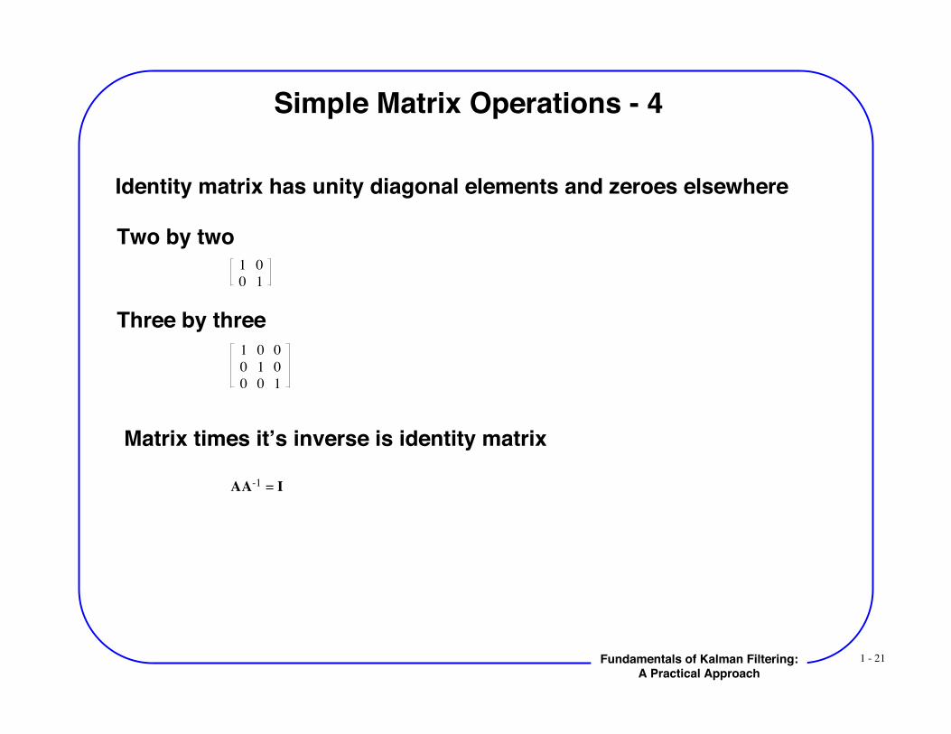
Simple Matrix Operations - 4
Identity matrix has unity diagonal elements and zeroes elsewhere
Two by two1 0
0 1
Three by three1 0 0
0 1 0
0 0 1
Matrix times itʼs inverse is identity matrix
AA-1 = I
1 - 22Fundamentals of Kalman Filtering:A Practical Approach
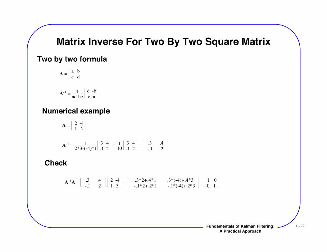
Matrix Inverse For Two By Two Square MatrixTwo by two formula
A = a b
c d
A-1 = 1
ad-bc
d -b
-c a
A = 2 -4
1 3
Numerical example
A-1 = 12*3-(-4)*1
3 4
-1 2 = 1
10 3 4
-1 2 = .3 .4
-.1 .2
Check
A-1A = .3 .4
-.1 .2 2 -4
1 3 = .3*2+.4*1 .3*(-4)+.4*3
-.1*2+.2*1 -.1*(-4)+.2*3 = 1 0
0 1
1 - 23Fundamentals of Kalman Filtering:A Practical Approach
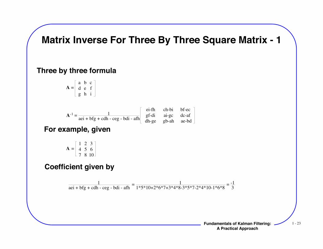
Three by three formula
A = a b c
d e f
g h i
Matrix Inverse For Three By Three Square Matrix - 1
A-1 = 1aei + bfg + cdh - ceg - bdi - afh
ei-fh ch-bi bf-ec
gf-di ai-gc dc-af
dh-ge gb-ah ae-bd
For example, given
A =
1 2 3
4 5 6
7 8 10
Coefficient given by
1aei + bfg + cdh - ceg - bdi - afh
= 11*5*10+2*6*7+3*4*8-3*5*7-2*4*10-1*6*8
= -13
1 - 24Fundamentals of Kalman Filtering:A Practical Approach
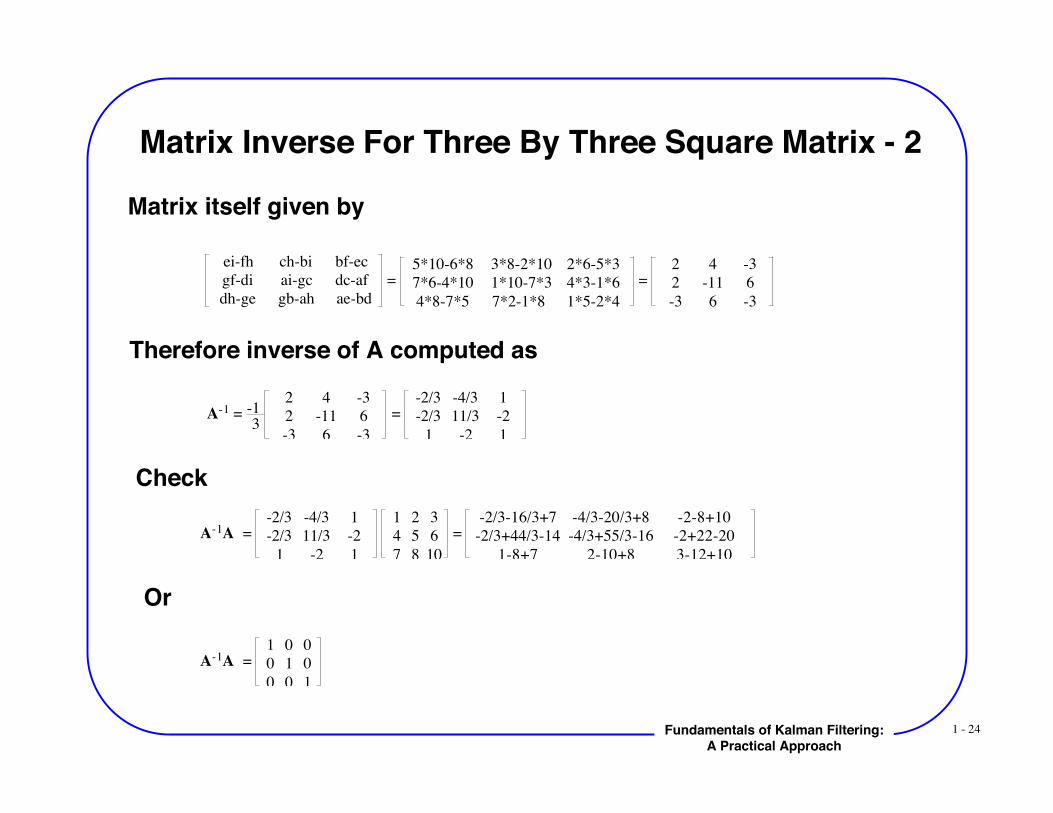
Matrix Inverse For Three By Three Square Matrix - 2
Matrix itself given by
ei-fh ch-bi bf-ec
gf-di ai-gc dc-af
dh-ge gb-ah ae-bd
= 5*10-6*8 3*8-2*10 2*6-5*3
7*6-4*10 1*10-7*3 4*3-1*6
4*8-7*5 7*2-1*8 1*5-2*4
= 2 4 -3
2 -11 6
-3 6 -3
Therefore inverse of A computed as
A-1 = -1
3
2 4 -3
2 -11 6
-3 6 -3
=
-2/3 -4/3 1
-2/3 11/3 -2
1 -2 1
Check
A-1A =
-2/3 -4/3 1
-2/3 11/3 -2
1 -2 1
1 2 3
4 5 6
7 8 10
=
-2/3-16/3+7 -4/3-20/3+8 -2-8+10
-2/3+44/3-14 -4/3+55/3-16 -2+22-20
1-8+7 2-10+8 3-12+10
Or
A-1A =
1 0 0
0 1 0
0 0 1
1 - 25Fundamentals of Kalman Filtering:A Practical Approach
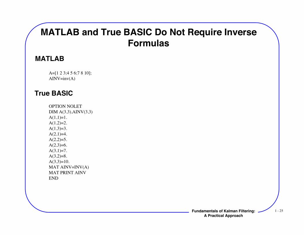
MATLAB and True BASIC Do Not Require InverseFormulas
MATLAB
A=[1 2 3;4 5 6;7 8 10];AINV=inv(A)
True BASICOPTION NOLETDIM A(3,3),AINV(3,3)A(1,1)=1.A(1,2)=2.A(1,3)=3.A(2,1)=4.A(2,2)=5.A(2,3)=6.A(3,1)=7.A(3,2)=8.A(3,3)=10.MAT AINV=INV(A)MAT PRINT AINVEND
1 - 26Fundamentals of Kalman Filtering:A Practical Approach
Numerical Integration of Differential Equations
1 - 27Fundamentals of Kalman Filtering:A Practical Approach
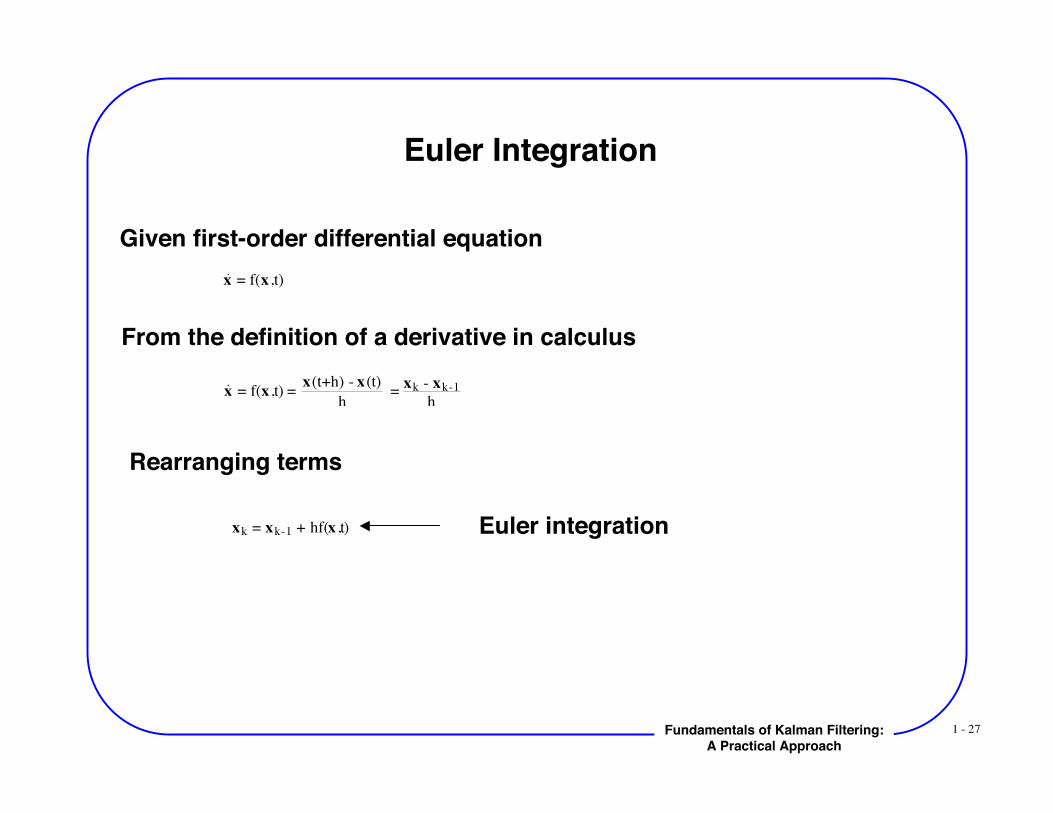
Euler Integration
Given first-order differential equationx = f(x ,t)
From the definition of a derivative in calculus
x = f(x,t) = x(t+h) - x(t)
h =
xk - xk-1
h
Rearranging terms
xk = xk-1 + hf(x ,t) Euler integration
1 - 28Fundamentals of Kalman Filtering:A Practical Approach
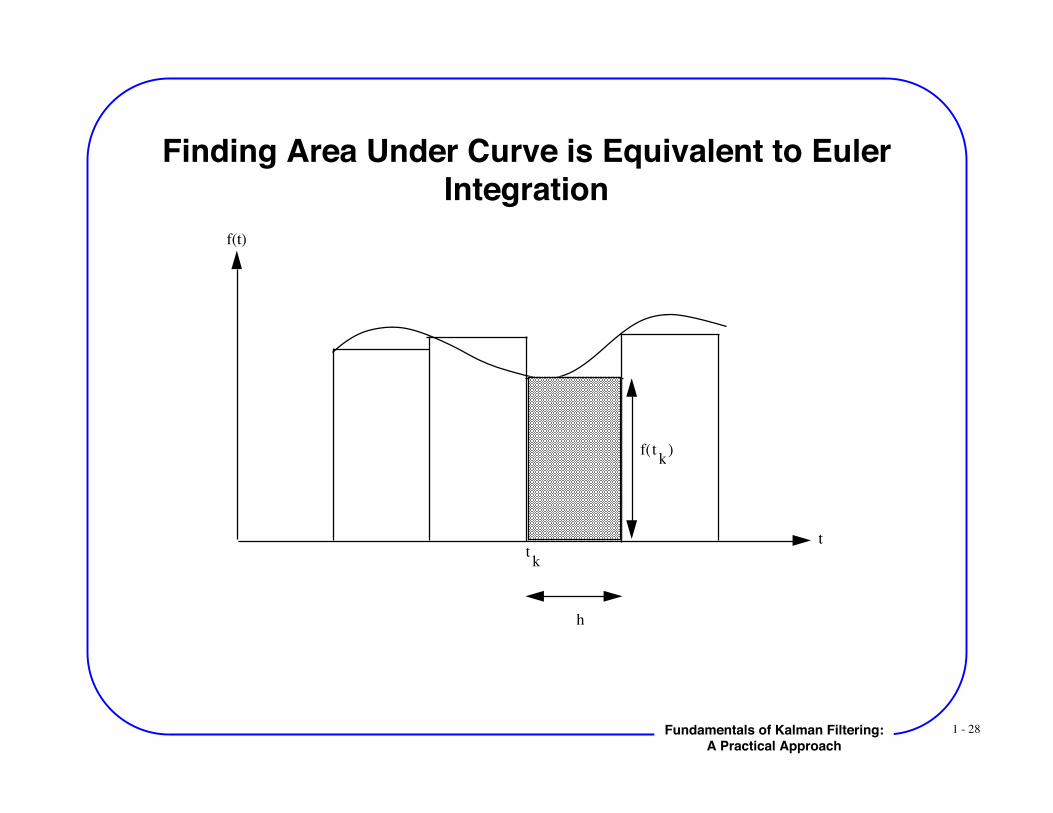
Finding Area Under Curve is Equivalent to EulerIntegration
h
t
f(t)
tk
f(tk)
1 - 29Fundamentals of Kalman Filtering:A Practical Approach
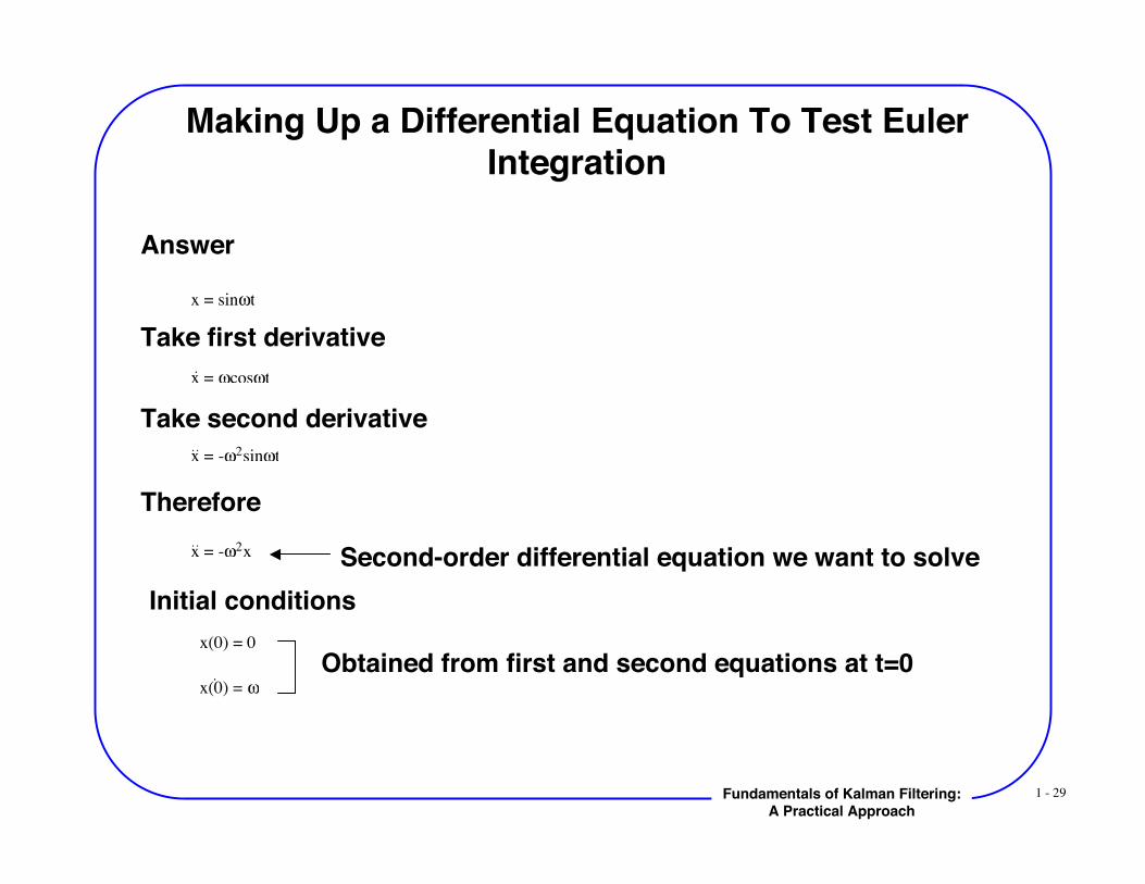
Making Up a Differential Equation To Test EulerIntegration
Answer
x = sin!t
Take first derivativex = !cos!t
Take second derivativex = -!2sin!t
Thereforex = -!2
x Second-order differential equation we want to solveInitial conditions
x(0) = 0
x(0) = !
Obtained from first and second equations at t=0
1 - 30Fundamentals of Kalman Filtering:A Practical Approach
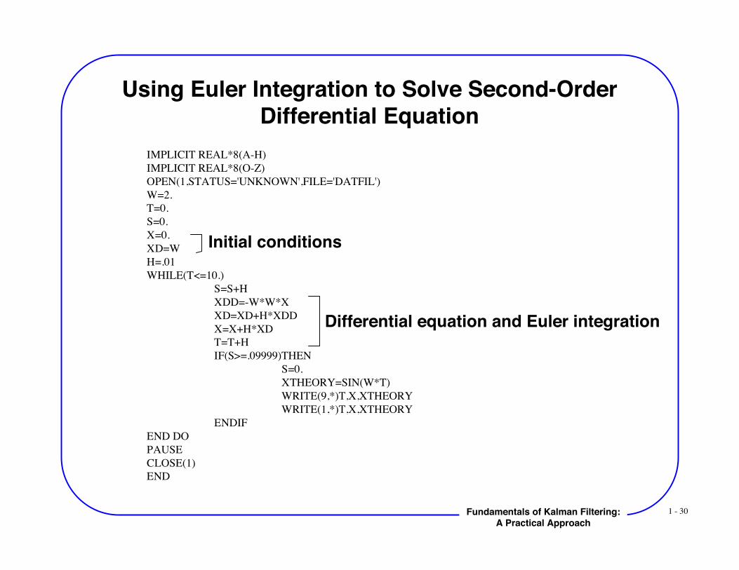
Using Euler Integration to Solve Second-OrderDifferential Equation
IMPLICIT REAL*8(A-H)IMPLICIT REAL*8(O-Z)OPEN(1,STATUS='UNKNOWN',FILE='DATFIL')W=2.T=0.S=0.X=0.XD=WH=.01WHILE(T<=10.)
S=S+HXDD=-W*W*XXD=XD+H*XDDX=X+H*XDT=T+HIF(S>=.09999)THEN
S=0.XTHEORY=SIN(W*T)WRITE(9,*)T,X,XTHEORYWRITE(1,*)T,X,XTHEORY
ENDIFEND DO
PAUSECLOSE(1)END
Differential equation and Euler integration
Initial conditions
1 - 31Fundamentals of Kalman Filtering:A Practical Approach
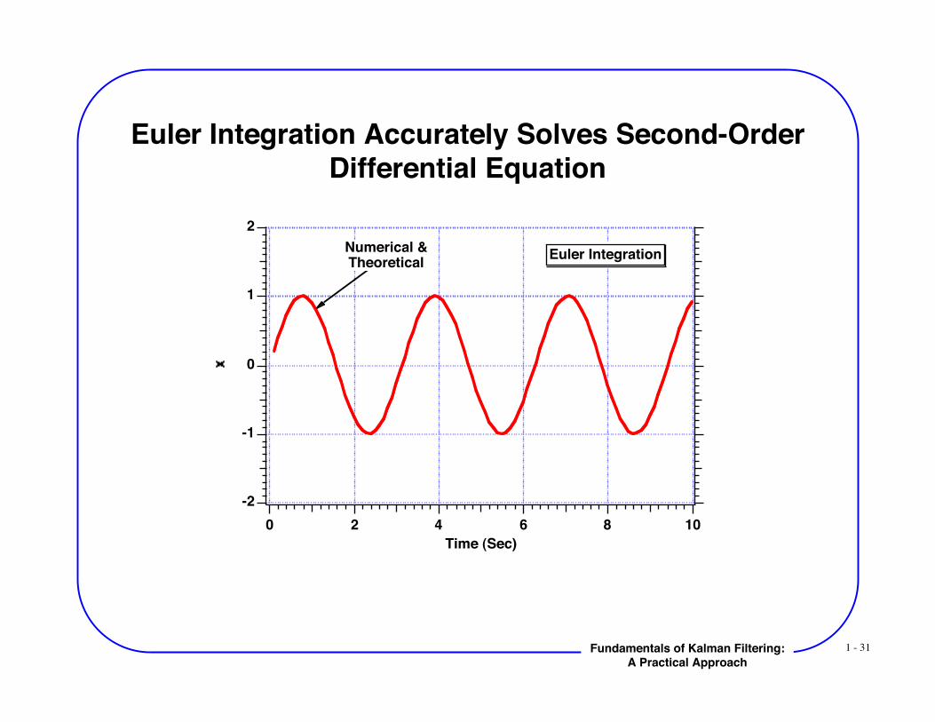
Euler Integration Accurately Solves Second-OrderDifferential Equation
-2
-1
0
1
2
1086420
Time (Sec)
Euler IntegrationNumerical &Theoretical
1 - 32Fundamentals of Kalman Filtering:A Practical Approach
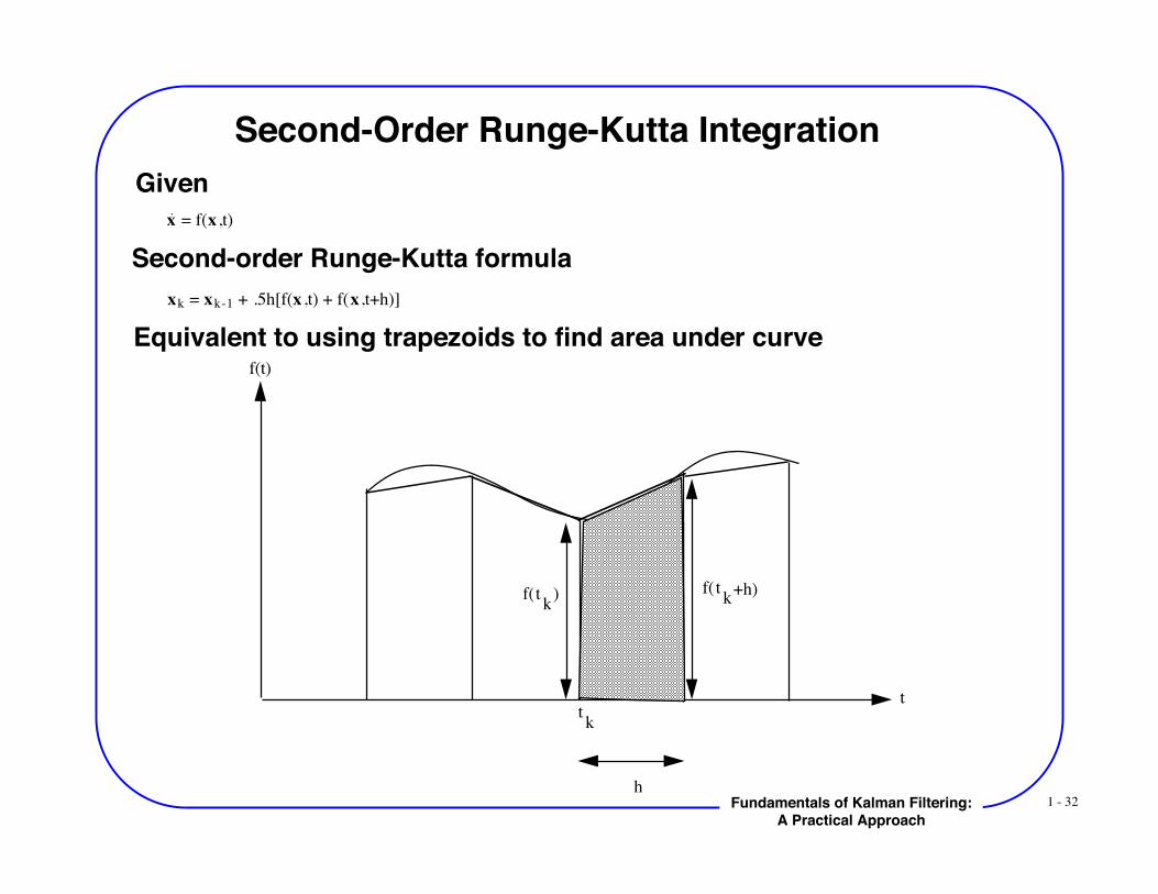
Second-Order Runge-Kutta IntegrationGiven
x = f(x ,t)
Second-order Runge-Kutta formulaxk = xk-1 + .5h[f(x ,t) + f(x ,t+h)]
h
t
f(t)
tk
f(tk) f( t
k+h)
Equivalent to using trapezoids to find area under curve

1 - 33Fundamentals of Kalman Filtering:A Practical Approach
Using Second-Order Runge-Kutta Integration toSolve Same Differential Equation
IMPLICIT REAL*8(A-H)IMPLICIT REAL*8(O-Z)OPEN(1,STATUS='UNKNOWN',FILE='DATFIL')W=2.T=0.S=0.X=0.XD=WH=.01
WHILE(T<=10.)S=S+HXOLD=XXDOLD=XDXDD=-W*W*XX=X+H*XDXD=XD+H*XDDT=T+HXDD=-W*W*XX=.5*(XOLD+X+H*XD)XD=.5*(XDOLD+XD+H*XDD)IF(S>=.09999)THEN
S=0.XTHEORY=SIN(W*T)WRITE(9,*)T,X,XTHEORYWRITE(1,*)T,X,XTHEORY
ENDIF END DO
PAUSECLOSE(1)END
Initial conditions
Second-order Runge-Kuttaintegration
1 - 34Fundamentals of Kalman Filtering:A Practical Approach
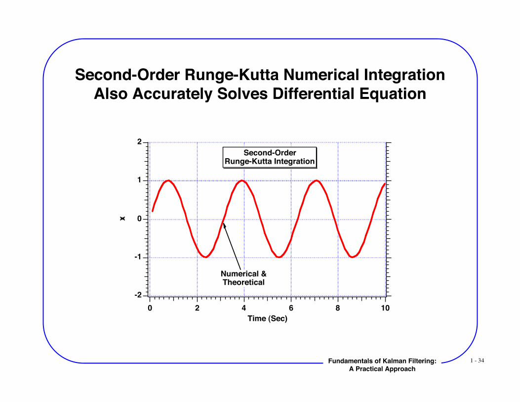
Second-Order Runge-Kutta Numerical IntegrationAlso Accurately Solves Differential Equation
-2
-1
0
1
2
1086420
Time (Sec)
Second-OrderRunge-Kutta Integration
Numerical &Theoretical
1 - 35Fundamentals of Kalman Filtering:A Practical Approach
Noise and Random Variables
1 - 36Fundamentals of Kalman Filtering:A Practical Approach
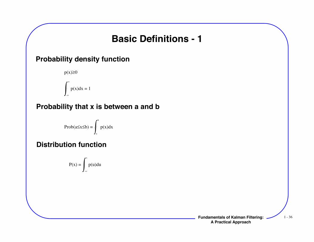
Basic Definitions - 1
Probability density functionp(x)!0
p(x)dx = 1
-!
!
Probability that x is between a and b
Distribution function
P(x) = p(u)du
-!
x
Prob(a!x!b) = p(x)dx
a
b
1 - 37Fundamentals of Kalman Filtering:A Practical Approach
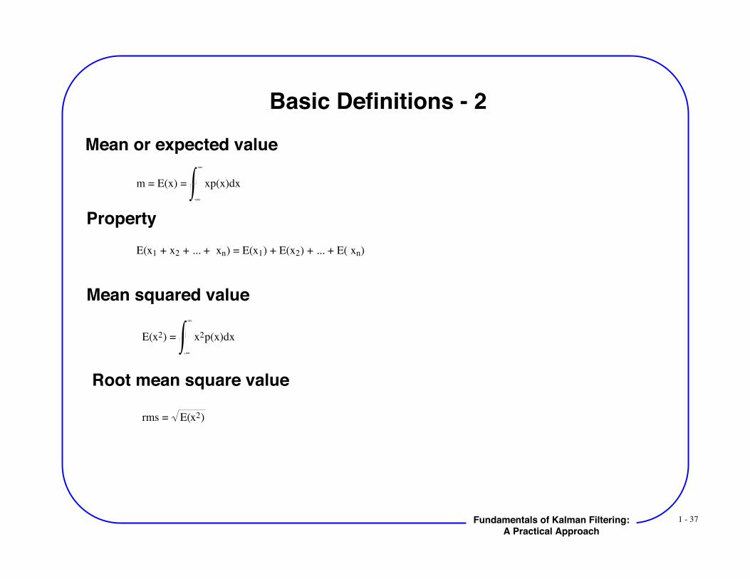
Basic Definitions - 2Mean or expected value
m = E(x) = xp(x)dx
-!
!
PropertyE(x1 + x2 + ... + xn) = E(x1) + E(x2) + ... + E( xn)
Mean squared value
E(x2) = x2p(x)dx
-!
!
Root mean square value
rms = E(x2)
1 - 38Fundamentals of Kalman Filtering:A Practical Approach
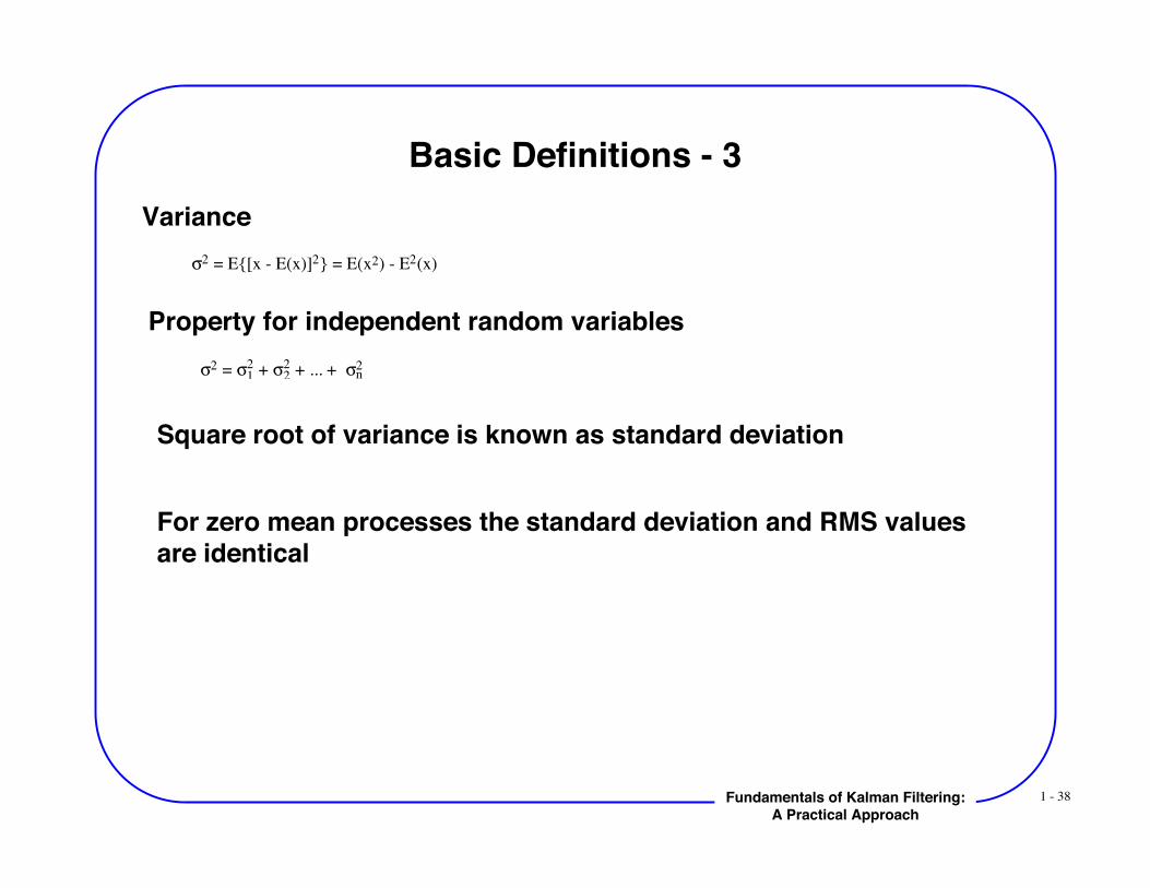
Basic Definitions - 3Variance
!2 = E{[x - E(x)]2} = E(x2) - E2(x)
Property for independent random variables!2 = !
1
2 + !
2
2 + ... + !n
2
Square root of variance is known as standard deviation
For zero mean processes the standard deviation and RMS valuesare identical
1 - 39Fundamentals of Kalman Filtering:A Practical Approach
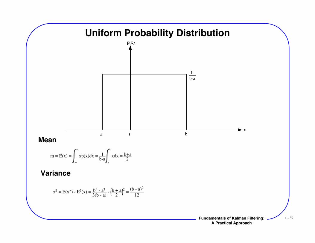
Uniform Probability Distribution
Mean
Variance
m = E(x) = xp(x)dx
-!
!
= 1b-a
xdx = b+a2
a
b
!2 = E(x2) - E2(x) = b3 - a3
3(b - a) - b + a
2
2 =
(b - a)2
12
1 - 40Fundamentals of Kalman Filtering:A Practical Approach
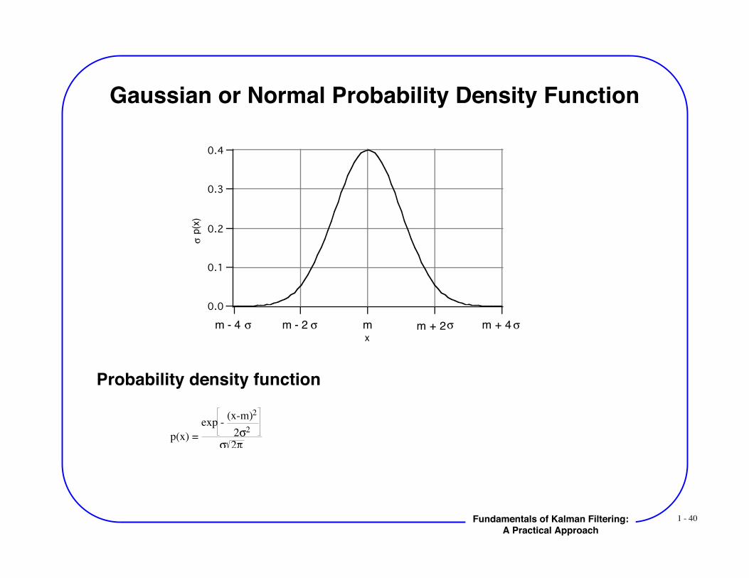
Gaussian or Normal Probability Density Function
0.4
0.3
0.2
0.1
0.0
! p(x
)
x
m - 4 ! !m - 2 m !m + 2 !m + 4
Probability density function
p(x) =
exp - (x-m)2
2!2
! 2"
1 - 41Fundamentals of Kalman Filtering:A Practical Approach
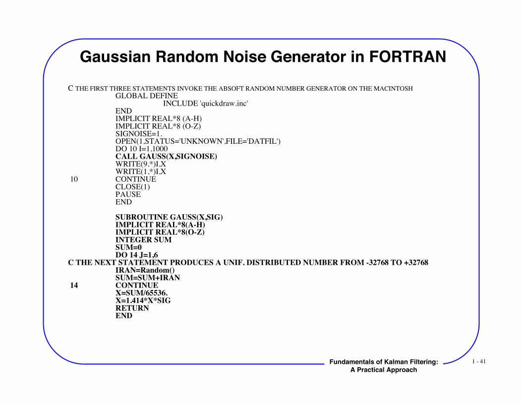
Gaussian Random Noise Generator in FORTRANC THE FIRST THREE STATEMENTS INVOKE THE ABSOFT RANDOM NUMBER GENERATOR ON THE MACINTOSH
GLOBAL DEFINE INCLUDE 'quickdraw.inc' END
IMPLICIT REAL*8 (A-H)IMPLICIT REAL*8 (O-Z)SIGNOISE=1.OPEN(1,STATUS='UNKNOWN',FILE='DATFIL')DO 10 I=1,1000CALL GAUSS(X,SIGNOISE)WRITE(9,*)I,XWRITE(1,*)I,X
10 CONTINUE CLOSE(1)
PAUSEEND
SUBROUTINE GAUSS(X,SIG)IMPLICIT REAL*8(A-H)IMPLICIT REAL*8(O-Z)INTEGER SUMSUM=0DO 14 J=1,6
C THE NEXT STATEMENT PRODUCES A UNIF. DISTRIBUTED NUMBER FROM -32768 TO +32768IRAN=Random()SUM=SUM+IRAN
14 CONTINUE X=SUM/65536.
X=1.414*X*SIGRETURNEND
1 - 42Fundamentals of Kalman Filtering:A Practical Approach
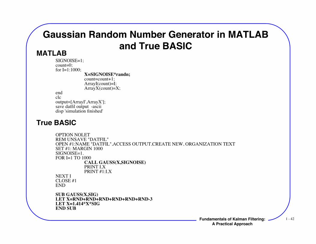
Gaussian Random Number Generator in MATLABand True BASIC
SIGNOISE=1;count=0;for I=1:1000;
X=SIGNOISE*randn;count=count+1;
ArrayI(count)=I; ArrayX(count)=X;endclcoutput=[ArrayI',ArrayX'];save datfil output -asciidisp 'simulation finished'
OPTION NOLETREM UNSAVE "DATFIL"OPEN #1:NAME "DATFIL",ACCESS OUTPUT,CREATE NEW, ORGANIZATION TEXTSET #1: MARGIN 1000SIGNOISE=1.FOR I=1 TO 1000
CALL GAUSS(X,SIGNOISE)PRINT I,XPRINT #1:I,X
NEXT ICLOSE #1END
SUB GAUSS(X,SIG)LET X=RND+RND+RND+RND+RND+RND-3LET X=1.414*X*SIGEND SUB
MATLAB
True BASIC
1 - 43Fundamentals of Kalman Filtering:A Practical Approach
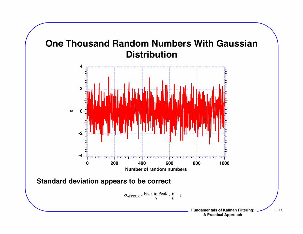
One Thousand Random Numbers With GaussianDistribution
!APPROX " Peak to Peak
6 " 6
6 = 1
Standard deviation appears to be correct
-4
-2
0
2
4
10008006004002000
Number of random numbers
1 - 44Fundamentals of Kalman Filtering:A Practical Approach
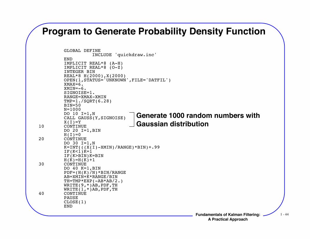
Program to Generate Probability Density Function
GLOBAL DEFINE INCLUDE 'quickdraw.inc' END
IMPLICIT REAL*8 (A-H)IMPLICIT REAL*8 (O-Z)INTEGER BINREAL*8 H(2000),X(2000)OPEN(1,STATUS='UNKNOWN',FILE='DATFIL')XMAX=6.XMIN=-6.SIGNOISE=1.RANGE=XMAX-XMINTMP=1./SQRT(6.28)BIN=50N=1000DO 10 I=1,NCALL GAUSS(Y,SIGNOISE)X(I)=Y
10 CONTINUE DO 20 I=1,BIN
H(I)=0 20 CONTINUE DO 30 I=1,N
K=INT(((X(I)-XMIN)/RANGE)*BIN)+.99IF(K<1)K=1IF(K>BIN)K=BINH(K)=H(K)+1
30 CONTINUE DO 40 K=1,BIN
PDF=(H(K)/N)*BIN/RANGEAB=XMIN+K*RANGE/BINTH=TMP*EXP(-AB*AB/2.)WRITE(9,*)AB,PDF,THWRITE(1,*)AB,PDF,TH
40 CONTINUEPAUSECLOSE(1)END
Generate 1000 random numbers withGaussian distribution
1 - 45Fundamentals of Kalman Filtering:A Practical Approach
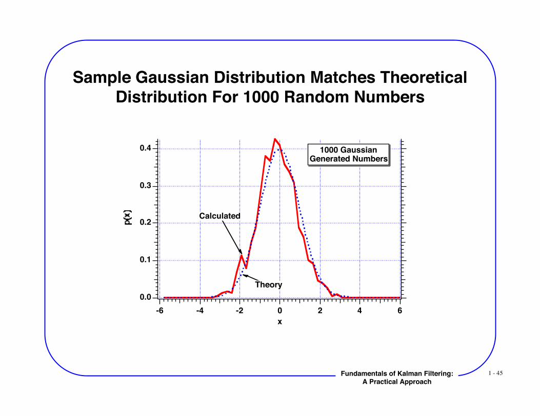
Sample Gaussian Distribution Matches TheoreticalDistribution For 1000 Random Numbers
0.4
0.3
0.2
0.1
0.0
-6 -4 -2 0 2 4 6
x
1000 GaussianGenerated Numbers
Calculated
Theory
1 - 46Fundamentals of Kalman Filtering:A Practical Approach
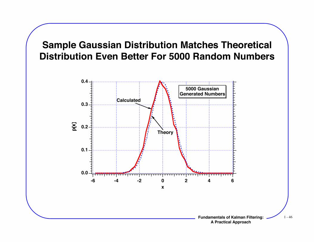
Sample Gaussian Distribution Matches TheoreticalDistribution Even Better For 5000 Random Numbers
0.4
0.3
0.2
0.1
0.0
-6 -4 -2 0 2 4 6
x
5000 GaussianGenerated Numbers
Calculated
Theory
1 - 47Fundamentals of Kalman Filtering:A Practical Approach
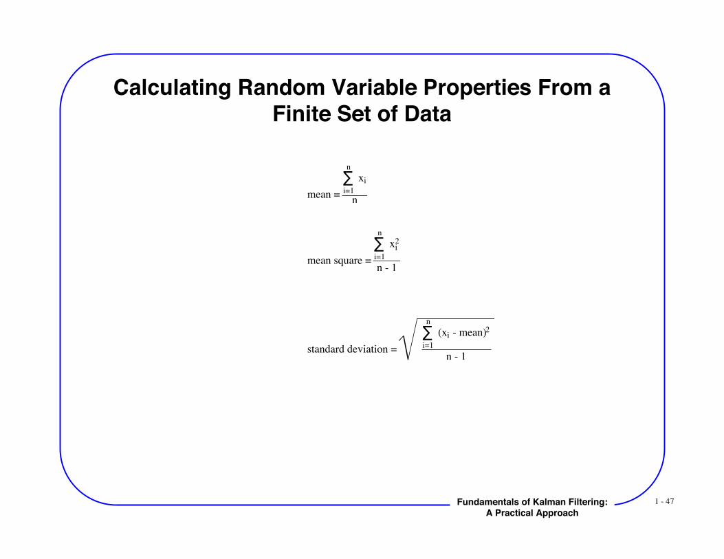
Calculating Random Variable Properties From aFinite Set of Data
mean =
xi!i=1
n
n
mean square =
xi2!
i=1
n
n - 1
standard deviation =
(xi - mean)2!i=1
n
n - 1
1 - 48Fundamentals of Kalman Filtering:A Practical Approach
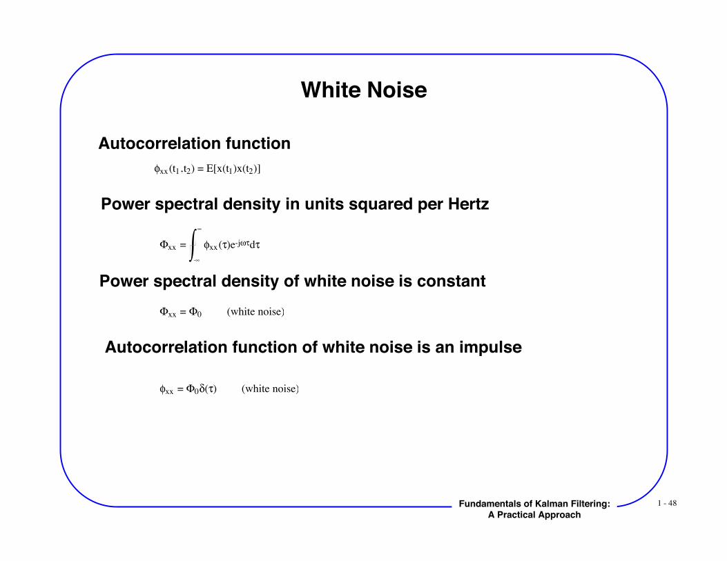
White Noise
Autocorrelation function!xx(t1,t2) = E[x(t1)x(t2)]
Power spectral density in units squared per Hertz
!xx = "xx(#)e-j$#d#
-%
%
Power spectral density of white noise is constant!xx = !0 (white noise)
Autocorrelation function of white noise is an impulse
!xx = "0#($) (white noise)
1 - 49Fundamentals of Kalman Filtering:A Practical Approach
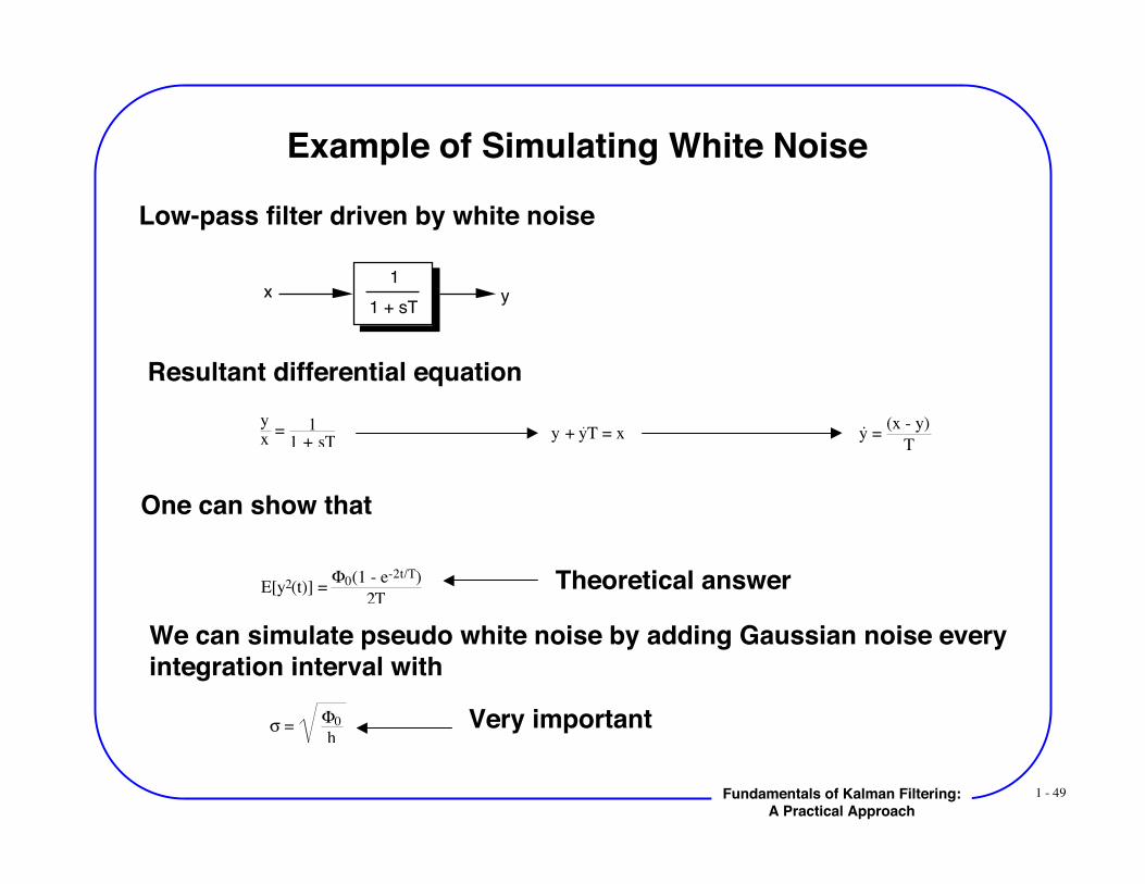
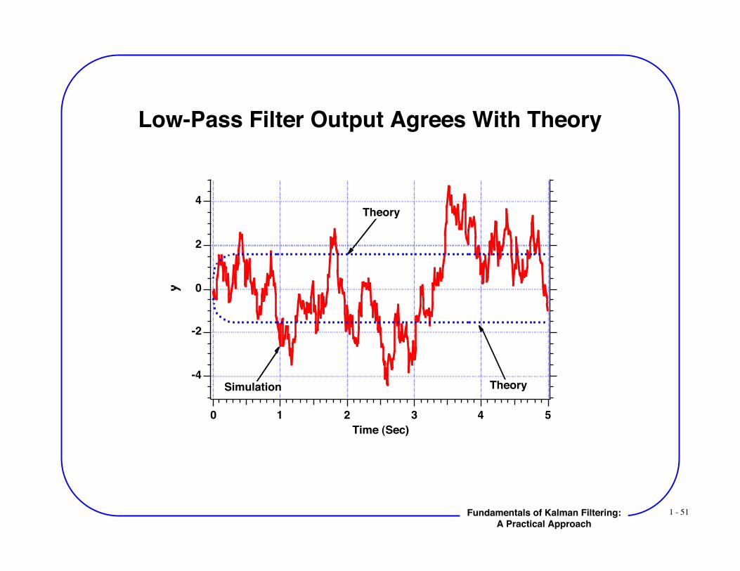
Example of Simulating White Noise
Low-pass filter driven by white noise
1
1 + sTx y
Resultant differential equation
y = (x - y)
T
One can show that
E[y2(t)] = !0(1 - e-2t/T)
2TTheoretical answer
We can simulate pseudo white noise by adding Gaussian noise everyintegration interval with
! = "0
h
Very important
yx
= 11 + sT
y + yT = x
1 - 50Fundamentals of Kalman Filtering:A Practical Approach
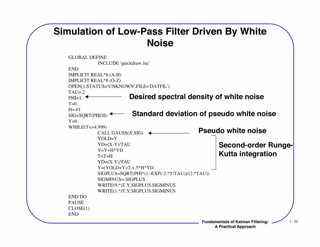
Simulation of Low-Pass Filter Driven By WhiteNoise
GLOBAL DEFINE INCLUDE 'quickdraw.inc' END
IMPLICIT REAL*8 (A-H)IMPLICIT REAL*8 (O-Z)OPEN(1,STATUS='UNKNOWN',FILE='DATFIL')TAU=.2PHI=1.T=0.H=.01SIG=SQRT(PHI/H)Y=0.
WHILE(T<=4.999) CALL GAUSS(X,SIG) YOLD=Y
YD=(X-Y)/TAU Y=Y+H*YD
T=T+HYD=(X-Y)/TAU
Y=(YOLD+Y)/2.+.5*H*YDSIGPLUS=SQRT(PHI*(1.-EXP(-2.*T/TAU))/(2.*TAU))SIGMINUS=-SIGPLUSWRITE(9,*)T,Y,SIGPLUS,SIGMINUSWRITE(1,*)T,Y,SIGPLUS,SIGMINUS
END DO PAUSE
CLOSE(1)END
Pseudo white noise
Second-order Runge-Kutta integration
Standard deviation of pseudo white noise
Desired spectral density of white noise
1 - 51Fundamentals of Kalman Filtering:A Practical Approach
Low-Pass Filter Output Agrees With Theory
-4
-2
0
2
4
543210
Time (Sec)
Simulation
Theory
Theory

1 - 52Fundamentals of Kalman Filtering:A Practical Approach
State Space Notation
1 - 53Fundamentals of Kalman Filtering:A Practical Approach
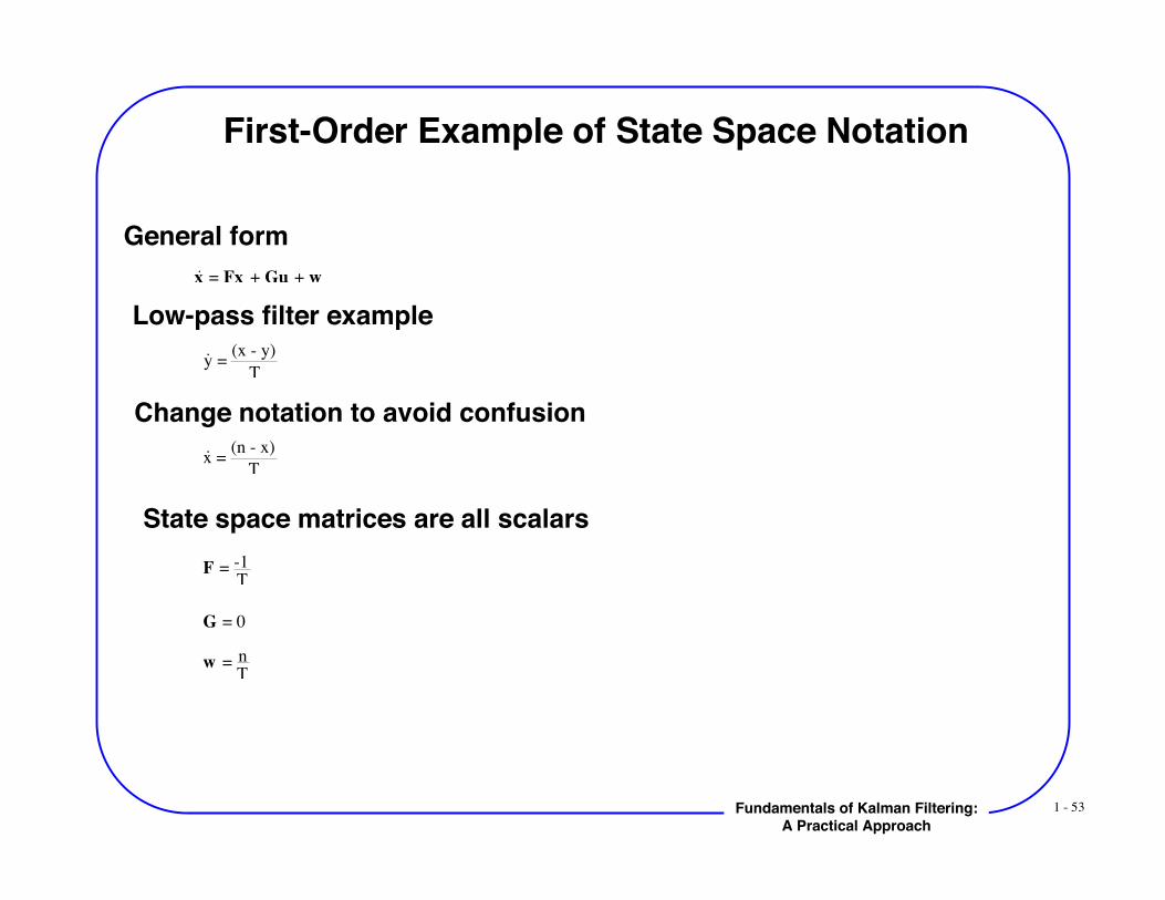
First-Order Example of State Space Notation
General formx = Fx + Gu + w
Low-pass filter exampley =
(x - y)
T
Change notation to avoid confusionx =
(n - x)
T
State space matrices are all scalars
G = 0
w = n
T
F = -1
T
1 - 54Fundamentals of Kalman Filtering:A Practical Approach
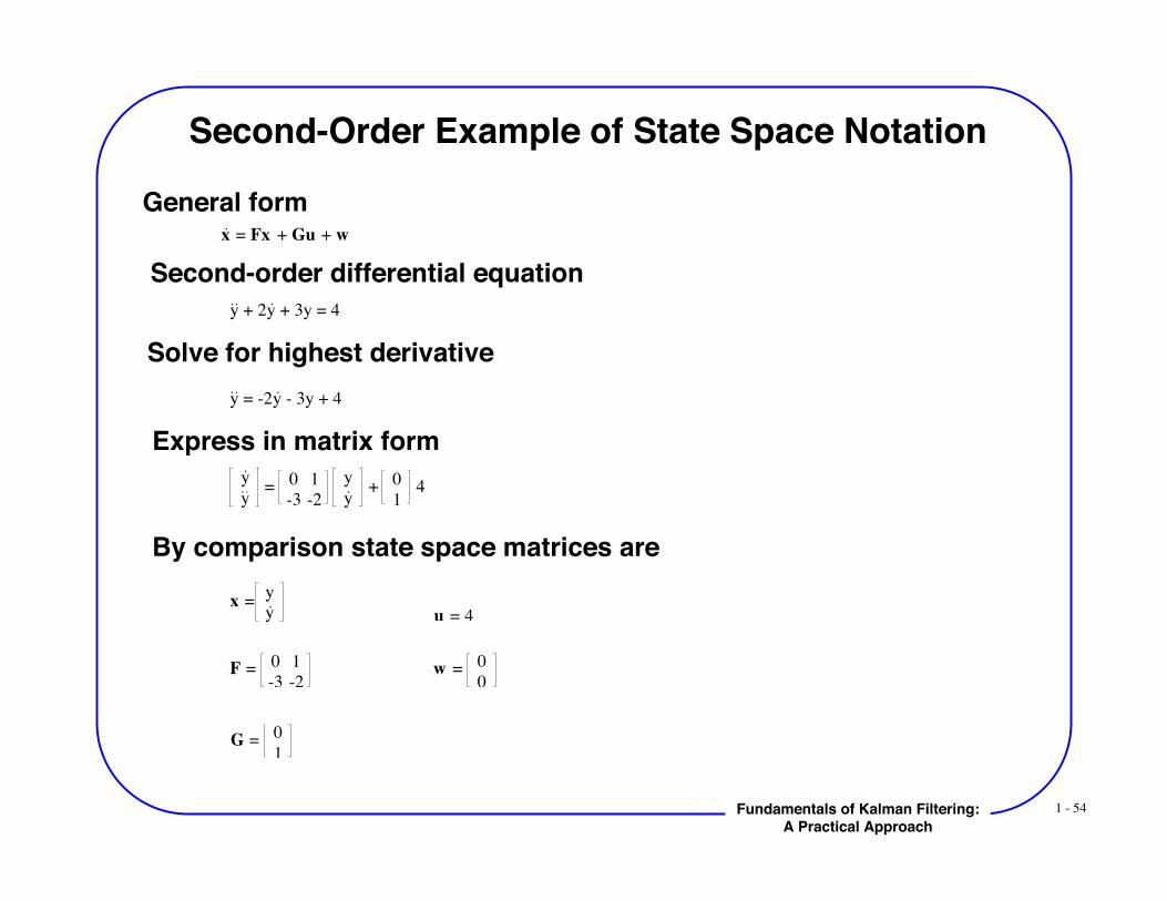
Second-Order Example of State Space Notation
General formx = Fx + Gu + w
Second-order differential equationy + 2y + 3y = 4
Solve for highest derivativey = -2y - 3y + 4
Express in matrix formy
y = 0 1
-3 -2
y
y + 0
1 4
By comparison state space matrices are
x =y
y
F = 0 1
-3 -2
G = 0
1
u = 4
w = 0
0

1 - 55Fundamentals of Kalman Filtering:A Practical Approach
Fundamental Matrix
1 - 56Fundamentals of Kalman Filtering:A Practical Approach
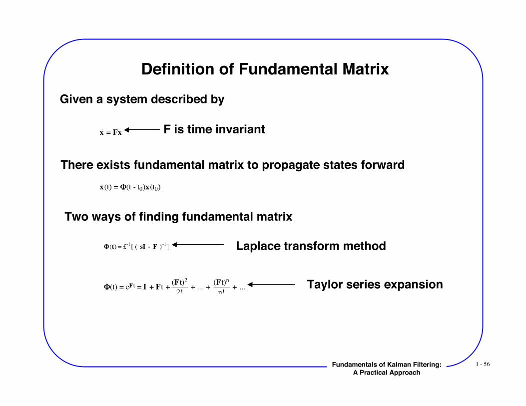
Definition of Fundamental MatrixGiven a system described by
x = Fx F is time invariant
There exists fundamental matrix to propagate states forwardx(t) = !(t - t0)x(t0)
Two ways of finding fundamental matrix
!(t) = £-1[ ( sI - F )
-1] Laplace transform method
!(t) = eFt = I + Ft + (Ft)2
2! + ... +
(Ft)n
n! + ... Taylor series expansion
1 - 57Fundamentals of Kalman Filtering:A Practical Approach
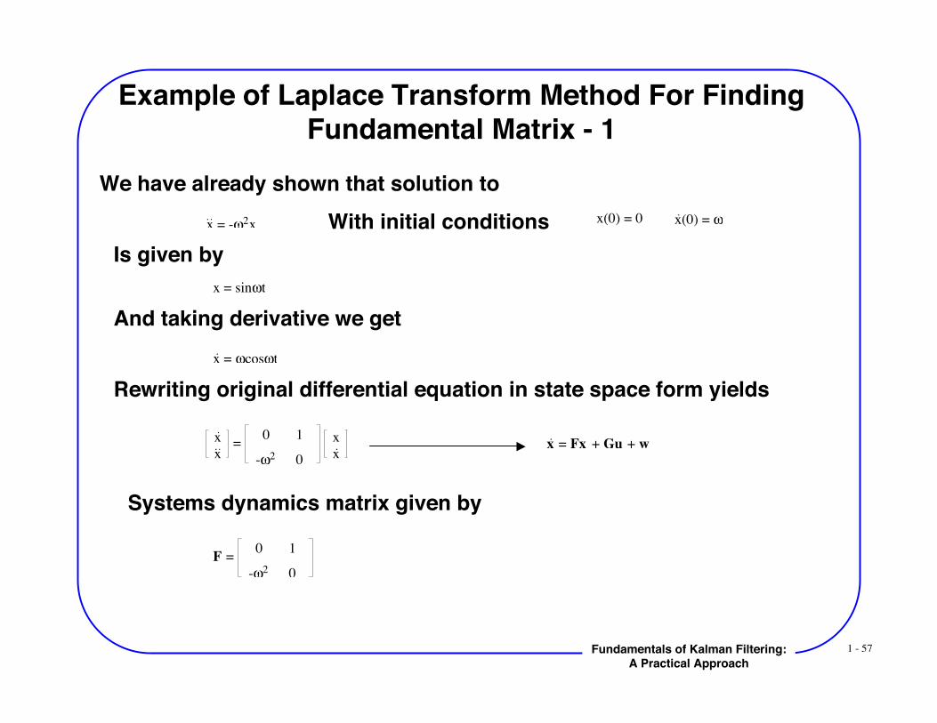
Example of Laplace Transform Method For FindingFundamental Matrix - 1
We have already shown that solution tox = -!2
x
Is given byx = sin!t
x = !cos!t
And taking derivative we get
Rewriting original differential equation in state space form yields
x
x =
0 1
-!2 0
x
xx = Fx + Gu + w
Systems dynamics matrix given by
F = 0 1
-!2 0
x(0) = 0 x(0) = !With initial conditions
1 - 58Fundamentals of Kalman Filtering:A Practical Approach
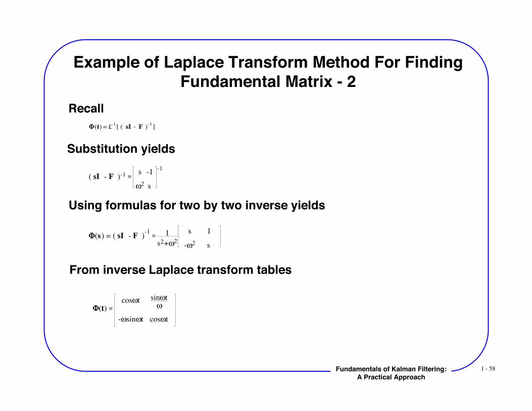
Example of Laplace Transform Method For FindingFundamental Matrix - 2
Recall!(t) = £
-1[ ( sI - F )
-1]
Substitution yields
Using formulas for two by two inverse yields
From inverse Laplace transform tables
!(t) =
cos"t sin"t"
-"sin"t cos"t
( sI - F )-1 = s -1
!2 s
-1
!(s) = ( sI - F )-1
= 1
s2+"2
s 1
-"2 s
1 - 59Fundamentals of Kalman Filtering:A Practical Approach
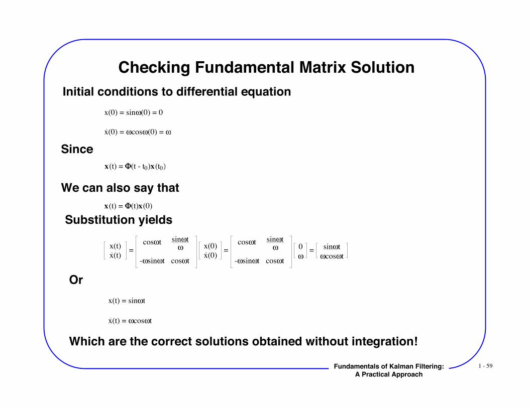
Checking Fundamental Matrix SolutionInitial conditions to differential equation
x(0) = sin!(0) = 0
x(0) = !cos!(0) = !
Sincex(t) = !(t - t0)x(t0)
We can also say thatx(t) = !(t)x(0)
Substitution yields
x(t)
x(t) =
cos!t sin!t!
-!sin!t cos!t
x(0)
x(0) =
cos!t sin!t!
-!sin!t cos!t
0
! = sin!t
!cos!t
Orx(t) = sin!t
x(t) = !cos!t
Which are the correct solutions obtained without integration!
1 - 60Fundamentals of Kalman Filtering:A Practical Approach
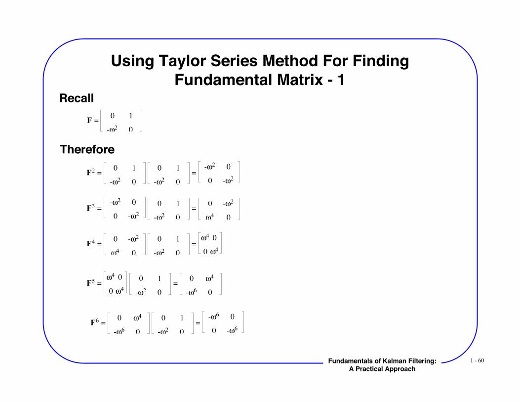
Using Taylor Series Method For FindingFundamental Matrix - 1
RecallF =
0 1
-!2 0
Therefore
F2 =
0 1
-!2 0
0 1
-!2 0
= -!2 0
0 -!2
F3 =
-!2 0
0 -!2
0 1
-!2 0
= 0 -!2
!4 0
F4 =
0 -!2
!4 0
0 1
-!2 0
= !4 0
0 !4
F5 =
!4 0
0 !4
0 1
-!2 0
= 0 !4
-!6 0
F6 =
0 !4
-!6 0
0 1
-!2 0
= -!6 0
0 -!6
1 - 61Fundamentals of Kalman Filtering:A Practical Approach
Using Taylor Series Method For FindingFundamental Matrix - 2
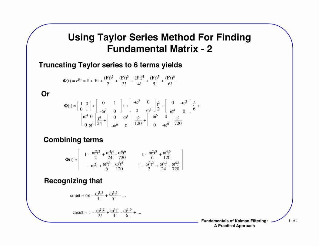
Truncating Taylor series to 6 terms yields
!(t) = eFt " I + Ft + (Ft)2
2! +
(Ft)3
3! +
(Ft)4
4! +
(Ft)5
5! +
(Ft)6
6!
Or !(t) " 1 0
0 1 +
0 1
-#2 0
t + -#2 0
0 -#2 t
2
2 +
0 -#2
#4 0
t3
6 +
#4 0
0 #4 t4
24 +
0 #4
-#6 0
t5
120 +
-#6 0
0 -#6 t6
720
Combining terms
!(t) "
1 - #2t2
2 + #
4t4
24 - #
6t6
720 t - #
2t3
6 + #
4t5
120
- #2t + #4t3
6 - #
6t5
120 1 - #
2t2
2 + #
4t4
24 - #
6t6
720
Recognizing that
sin!t " !t - !3t3
3! + !
5t5
5! - ...
cos!t " 1 - !2t2
2! + !
4t4
4! - !
6t6
6! + ...
1 - 62Fundamentals of Kalman Filtering:A Practical Approach
Using Taylor Series Method For FindingFundamental Matrix - 3
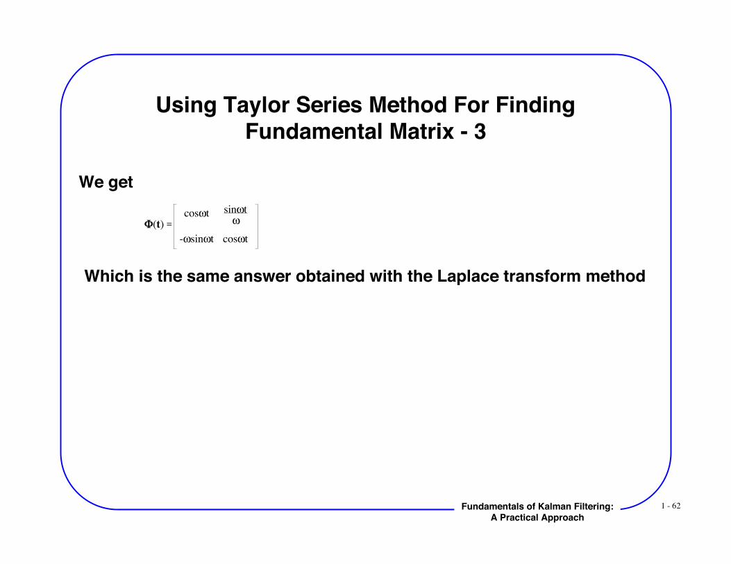
We get
!(t) =
cos"t sin"t"
-"sin"t cos"t
Which is the same answer obtained with the Laplace transform method
1 - 63Fundamentals of Kalman Filtering:A Practical Approach
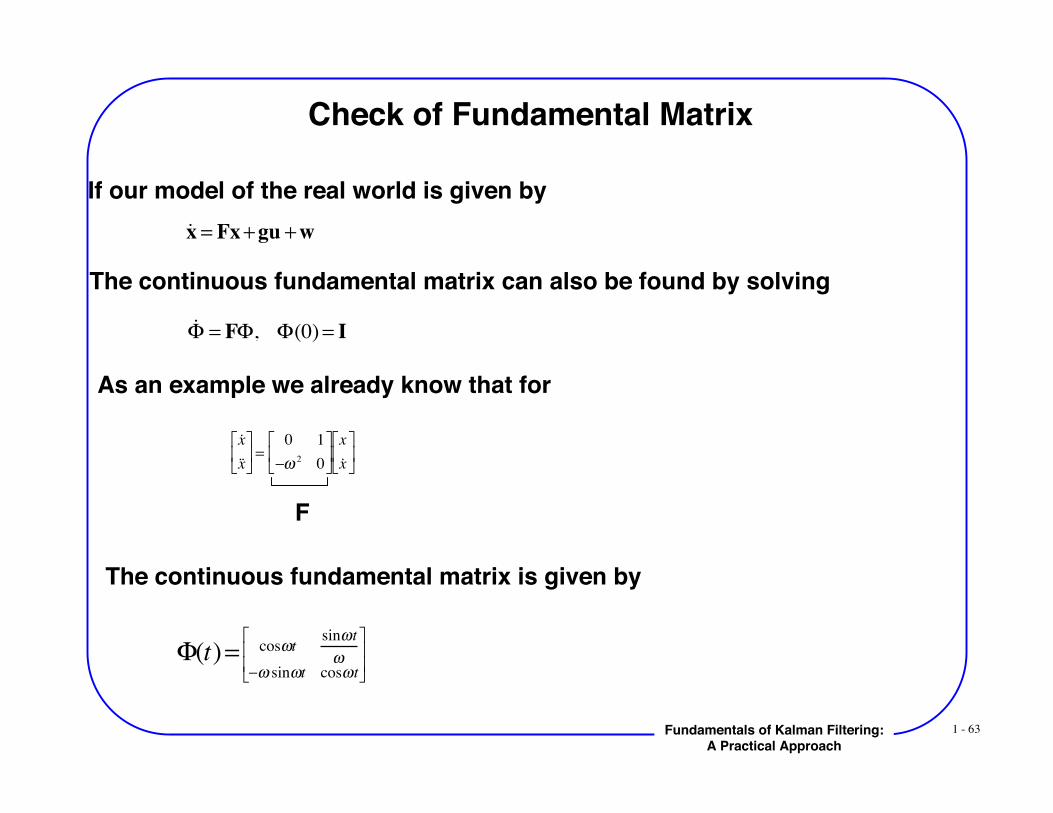
Check of Fundamental Matrix
If our model of the real world is given by
˙ x = Fx + gu + w
The continuous fundamental matrix can also be found by solving
˙ ! = F!, !(0) = I
As an example we already know that for
˙ x
˙ ̇ x
!
" #
$
% & =
0 1
'( 20
!
" #
$
% &
x
˙ x
!
" #
$
% &
The continuous fundamental matrix is given by
F
!(t)=cos"t
sin"t
"#" sin"t cos"t
$
%
&
&
'
(
)
)
1 - 64Fundamentals of Kalman Filtering:A Practical Approach
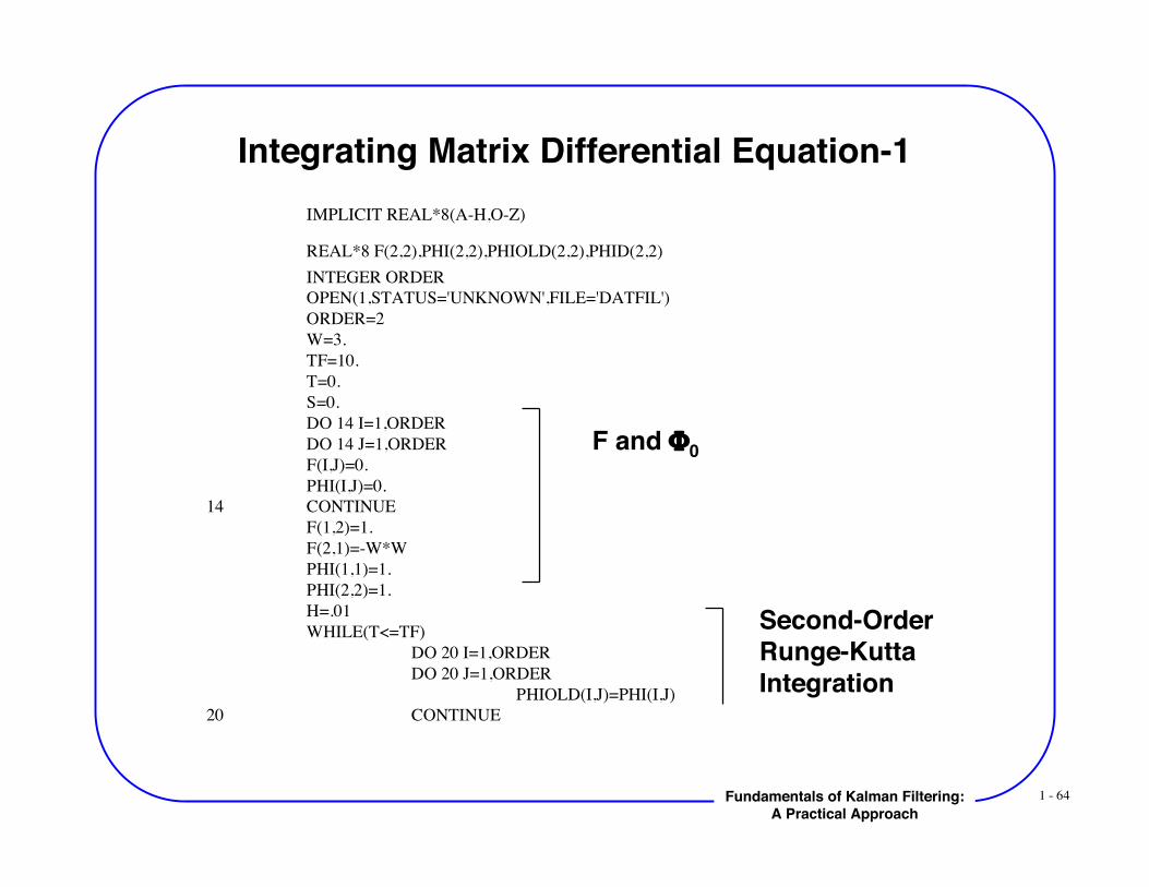
Integrating Matrix Differential Equation-1IMPLICIT REAL*8(A-H,O-Z)
REAL*8 F(2,2),PHI(2,2),PHIOLD(2,2),PHID(2,2)INTEGER ORDEROPEN(1,STATUS='UNKNOWN',FILE='DATFIL')ORDER=2W=3.TF=10.T=0.S=0.DO 14 I=1,ORDERDO 14 J=1,ORDERF(I,J)=0.PHI(I,J)=0.
14 CONTINUE F(1,2)=1. F(2,1)=-W*W
PHI(1,1)=1.PHI(2,2)=1.H=.01
WHILE(T<=TF)DO 20 I=1,ORDERDO 20 J=1,ORDER
PHIOLD(I,J)=PHI(I,J) 20 CONTINUE
F and Φ0
Second-OrderRunge-KuttaIntegration
1 - 65Fundamentals of Kalman Filtering:A Practical Approach
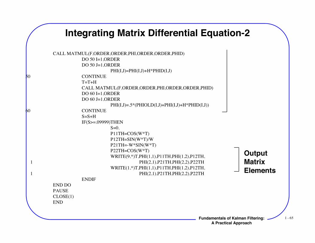
Integrating Matrix Differential Equation-2
OutputMatrixElements
CALL MATMUL(F,ORDER,ORDER,PHI,ORDER,ORDER,PHID)DO 50 I=1,ORDERDO 50 J=1,ORDER
PHI(I,J)=PHI(I,J)+H*PHID(I,J) 50 CONTINUE T=T+H
CALL MATMUL(F,ORDER,ORDER,PHI,ORDER,ORDER,PHID)DO 60 I=1,ORDERDO 60 J=1,ORDER
PHI(I,J)=.5*(PHIOLD(I,J)+PHI(I,J)+H*PHID(I,J)) 60 CONTINUE
S=S+HIF(S>=.09999)THEN
S=0.P11TH=COS(W*T)P12TH=SIN(W*T)/WP21TH=-W*SIN(W*T)P22TH=COS(W*T)WRITE(9,*)T,PHI(1,1),P11TH,PHI(1,2),P12TH,
1 PHI(2,1),P21TH,PHI(2,2),P22THWRITE(1,*)T,PHI(1,1),P11TH,PHI(1,2),P12TH,
1 PHI(2,1),P21TH,PHI(2,2),P22TH ENDIF
END DOPAUSECLOSE(1)END
1 - 66Fundamentals of Kalman Filtering:A Practical Approach
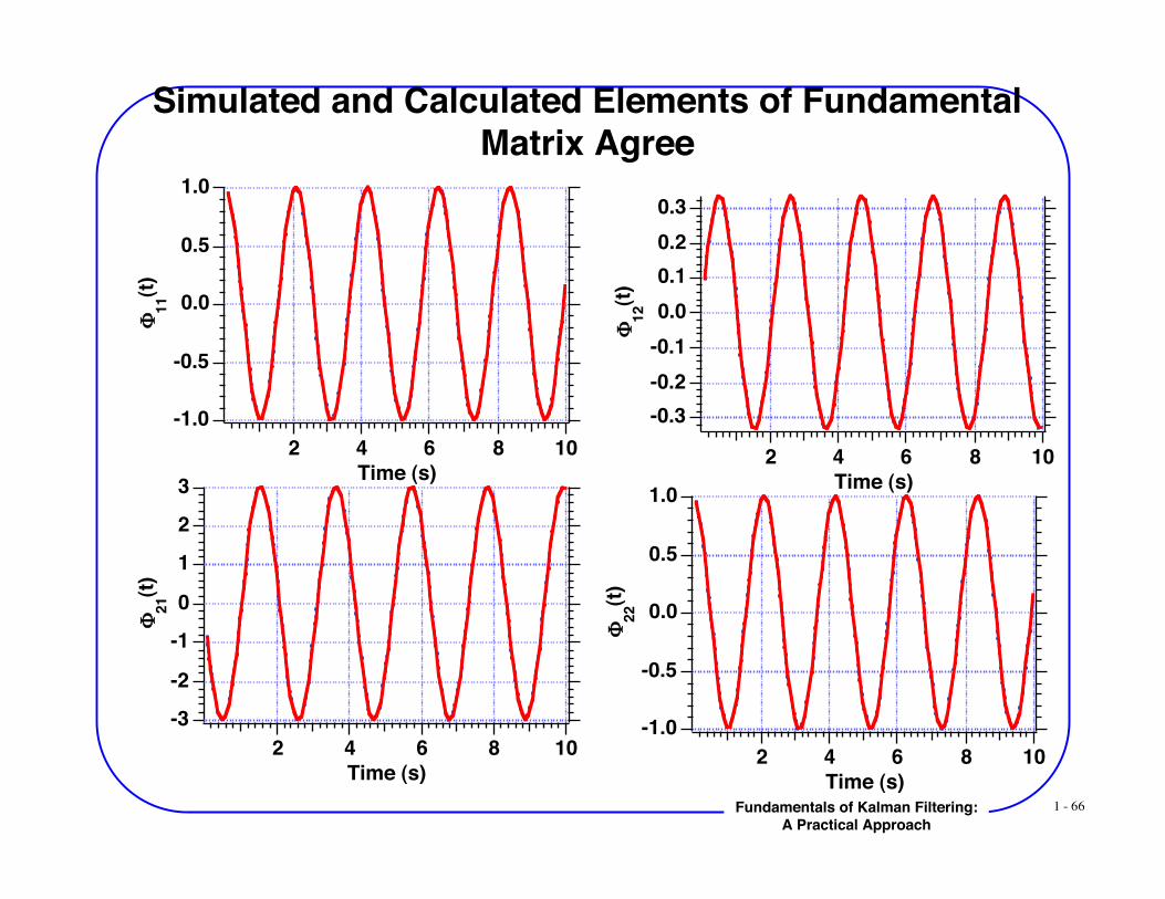
Simulated and Calculated Elements of FundamentalMatrix Agree
1.0
0.5
0.0
-0.5
-1.0
!11(t
)
108642
Time (s)
-3
-2
-1
0
1
2
3
!21(t
)
108642
Time (s)
0.3
0.2
0.1
0.0
-0.1
-0.2
-0.3
!12(t
)
108642
Time (s)1.0
0.5
0.0
-0.5
-1.0
!22(t
)
108642
Time (s)
1 - 67Fundamentals of Kalman Filtering:A Practical Approach
Numerical BasicsSummary
• Vector and matrix manipulations introduced and demonstrated
• Numerical integration techniques presented and verified
• Source code can easily be converted to other languages
• State space concepts and fundamental matrix introduced