FUNDAMENTALS OF CALCULATION OF EARTH … Sheath Bonding Application... · EARTH POTENTIAL RISE IN THE UNDERGROUND POWER DISTRIBUTION CABLE ... The calculation of sequence impedances

Companion Document to NZCCPTS Application Guide

for Cable Sheath Bonding

FUNDAMENTALS OF CALCULATION OF EARTH POTENTIAL RISE IN THE UNDERGROUND POWER DISTRIBUTION CABLE

NETWORK

Ashok Parsotam

March 1997

Reprinted 2003

2

Foreword This paper provides a detailed outline of how to calculate the fault currents and earth potential rise that will result when a high voltage cable between two substations has its sheath bonded to the substation earth mat at each end. The author, Ashok Parsotam, presented this paper at the “Power and Telecommunications Systems Co-ordination Conference”, Melbourne, on 19 March 1997. At the time he was an Engineer with Southpower. Ashok now works for Vector Limited. His contact details are: Ashok Parsotam Security Planning Engineer Vector Limited PO Box 99882 Newmarket AUCKLAND Ph: 0-9-529 8609 Fax: 0-9-529 8323 Email [email protected]

3

Power & Telecommunications Systems Coordination Conference

Bayside NOVOTEL, St. Kilda, Melbourne, Wednesday 19 March 1997

FUNDAMENTALS OF CALCULATION OF EARTH POTENTIAL RISE IN THE

UNDERGROUND POWER DISTRIBUTION CABLE NETWORK

BY

ASHOK K PARSOTAM

Project Engineer Planning Southpower Christchurch

NEW ZEALAND

Ph: +64 3 363 9750 Fax: +64 3 363 9707

Email: [email protected]

SUMMARY In this paper, the fundamentals of how to calculate earth potential rise (EPR) in an underground power distribution network are presented in some detail. The objective is to enable engineers with a basic knowledge of power system analysis to further develop their skills and understanding of EPR calculations in a typical distribution network. The calculation of sequence impedances to model overhead lines and underground cables and calculate the Earth Potential Rise in the cable network, is presented in some detail, to enable a Power Systems Engineer to understand and design cost effective earthing systems. This paper can be treated as a guide or a reference document for calculating the fault currents in a distribution network1. Several fault scenarios were modelled. For each model a numerical example outlining all steps required to calculate EPR is also provided. The equations given in this document can also be used for calculating line and cable series impedance parameters required by PTI’S Power System Simulator (PSS/U) and most other load flow and short circuit analysis software packages The methods and models presented in this paper are such that they can be readily applied to practical situations by a Power Systems Engineer using a basic scientific hand calculator.

1While the author has taken all reasonable care in compiling this paper, and satisfying himself as to the information in it, the author takes no responsibility whatsoever for any loss, expense, claim or damage suffered or incurred by any person who acts on reliance of any of the information contained in it. The author expressly disclaims all and any liability to any person, whether a purchaser of this paper or not, in respect of anything done or not done by that person in reliance either wholly or partly on the information contained in this paper.

4

For the 11kV cable network studied, the calculations show that even though 96% of the total fault current returns to the source via the cable sheath, the earth potential rise for a 10 Ohms earthing system can still be as high as 3100 Volts. This indicates that careful consideration should be given to the design of all earthing systems.

1. INTRODUCTION

The author has observed young graduate engineers using available computer programs to model substation earth mats and calculate earth potential rise (EPR) without understanding the importance of the parameters involved. In one instance, an engineer was calculating EPR for a 33/11kV zone substation earth mat. The calculated earth mat resistance was 3 Ohms, the source substation had an 11 Ohms neutral earthing resister and the length of the 33kV line to the zone substation was approximately 10km. This engineer used a 10kA fault current to simulate the substation earth potential rise and associated voltage contours. An engineer with some knowledge of power system fault analysis would have quickly worked out that the maximum phase to earth fault current (post transient steady state) at the source substation could not be greater than 33,000/(( 3 )(11 Ohm)) or 1732 amperes. Obviously, the EPR of a 3 Ohm earth mat with 1732 A fault current is only 5196 Volts compared to 30kV calculated by the earth mat analysis software. The author, in early days of exposure to such calculations, also made similar mistakes. His mistakes were associated with calculation of EPR in an 11kV underground cable network. The author had fault analysis software (PSSU) which had the facility to calculate high impedance phase to earth fault currents. He used this facility and calculated earth fault currents and EPR in a cable network and it was a mistake. The fault current calculated by PSSU was equal to the current in the faulty phase conductor and there was no way of finding out the proportions that returned to the source via the cable sheath and the general mass of earth. It was during these calculations the author realised that special considerations are required to calculate EPR in a cable network. The fundamental part of calculation of the earth potential rise is the calculation of the phase to earth fault current magnitude in a given network. This requires network impedance calculations, fault current analysis and then design of the earthing system to assess and control the hazardous EPR.

The fault current analysis of a 3-phase 3-wire overhead line distribution network is relatively simple compared to that of an underground cable network, or a combination of overhead and underground networks. In this paper, a method of calculating fault current split (between cable sheath and the general mass of earth), and the EPR and the transferred earth potential rise (TEPR) for the phase to earth faults in the overhead and the underground three core cable power distribution network will be presented.

2 EARTH POTENTIAL RISE This paper models underground cable and overhead line systems to calculate phase to earth fault current splits and EPR. In these models, the earth mat will be represented as a single lumped impedance element in the fault circuit network. The touch and step voltages associated with EPR can not be calculated explicitly in such models. However, it is possible to calculate the transferred EPR. The mathematical modelling of an earth mat for touch and step voltages inside and outside the confines of the earth mat is indeed a complex subject. The effective solution generally requires computer modelling. However, it is relatively easy to calculate EPR if the impedance of the earth mat is known.

5

3 CALCULATION OF SEQUENCE IMPEDANCES OF AN UNDERGROUND CABLE In order to calculate the fault current in a network, one must first calculate the impedance of the network elements. In this paper, the symmetrical components method of analysis for current split during phase to earth faults will be developed and used.

To use the symmetrical components method of analysis, the network elements (transformers, lines, cables and generators) impedance should be calculated or obtained from measurements. For a typical distribution network system analysis, the elements are transformers, lines and cables. However, in this paper, to simplify calculations, transformers are not explicitly modelled. This enables us to carry out calculations without the additional complexity of transformer turns ratio and hence the use of the per-unit system. The symmetrical components method of analysis is a convenient mathematical tool for the analysis of unbalanced network conditions. This method decomposes the unbalanced network parameters i.e. voltages and currents into three separate but balanced and symmetrical components, namely positive, negative and zero sequence components. Therefore, to calculate positive, negative and zero sequence voltages and currents, we must first calculate the corresponding positive, negative and zero sequence impedances which will generate and limit voltages and currents respectively. Extreme unbalances of voltages and currents in the network are caused by system faults such as phase to earth faults.

In the following sections, the equations for calculating the series positive and the zero sequence impedance values for a 3 core, insulated metallic sheath covered cables and 3-phase 3-wire short overhead lines are given and corresponding symmetrical components circuit models (for single phase to earth fault conditions) are developed.

The shunt admittance of the cables and the lines has been neglected from these calculations. In a later section, a comparison has been made between the results obtained using the models developed in this paper, and the models used in more sophisticated applications such as transient analysis.

The equations to calculate the cable and the line parameters were taken from the Wagner & Evans book (1). The derivation of these equations was shown in this book. And are in imperial units (inches, Ohm/mile) rather than metric units. The equations presented in this paper are an equivalent metric version of the original equations.

3.1 THE POSITIVE SEQUENCE IMPEDANCE OF THE 3-CORE INSULATED

METALLIC SHEATH COVERED CABLES In the following calculations, it is assumed that the cable sheath is insulated from the surrounding earth. Figure 3.1 below shows a cross section of a typical cable.

Fig. 3.1 Cross section of a typical underground cable. In this picture, the cable sheath is shown as electrically insulated from the ground.

6

3.1.1 Positive Sequence Resistance For such analysis at power frequency (i.e. 50 HZ), it can be assumed that the positive sequence AC resistance of the conductors is equal to the DC resistance of the conductor. R1=Rcond(DC) Ω/Ø/km eqn. 1

3.1.2 Positive Sequence Reactance The positive sequence reactance of the cable can be calculated from the following equation:

=Χ −

GMRSfx 10

31 log.10893.2 Ω/Ø/km eqn.2

where ƒ - frequency Hz S - separation of the conductors (in an equilateral triangle disposition), or the Geometric Mean Distance (GMD) of conductors in mm. See figure 3.1. GMR - is the Geometric Mean Radius of one conductor (mm) and is calculated by the following equation: GMR = (k a) mm eqn. 3 a radius of the conductor mm. See figure 3.1 k factor to convert the conductor radius to the Geometric mean Radius (GMR) of the conductor (See Table 3.1)

Conductor type K Solid round conductor 0.779

Full Stranding 7 0.726

19 0.758 37 0.768 61 0.772 91 0.774

127 0.776 Hollow stranded conductors and A.C.S.R. (Neglecting steel strands)

6 one layer 0.768** 30 two layer 0.826 36 two layer 0.809

54 three layer 0.810 Single layer A.C.S.R. 0.35 - 0.70

Point within circle to circle 1 Point outside circle to circle Distance to centre of circle Rectangular section of sides α and β 0.2235 (α + β)

Table 3.1 Geometric Mean Radii (GMR) factors for different Conductors. This table is from the Wagner & Evans book “Symmetrical Components” pg. 138 **The 6 one layer ASCR k factor was calculated by the author. The calculation is shown in appendix A. More information on calculation of GMR can be found in [2]. Hence, the positive sequence impedance of a 3 core cable (figure 3.1) is given by: Z1=R1+jX1 Ω/Ø/km eqn. 4

7

3.2 THE NEGATIVE SEQUENCE IMPEDANCE OF THE CABLE The negative sequence impedance of the cable is equal to the positive sequence impedance. Z2=Z1=R1+jX1 Ω/Ø/km

3.3 THE ZERO SEQUENCE IMPEDANCE OF THE CABLE 3.3.1 The Zero Sequence Self Impedance of the 3-Core Cable Conductors (Zsc0)

To calculate the zero sequence self impedance of the cable, the conductors in the cable must be considered as a group (see figure 3.2 below), and the equivalent GMR for the group of conductors must be calculated. Figure 3.2 The 3 conductors of the cable replaced by a single conductor with an equivalent GMR and resistance of 3 parallel conductors considered as group. The equation to calculate the zero sequence self impedance is given below.

Zsc0

++ −−

cond

cond

GMRf

fxjfxR

310

36658368

log10893.2102.9883

ρ

Ω/Ø/km eqn.5

where Rcond - DC Resistance of one conductor (Ω/km) f - frequency (Hz) ρ - deep layer soil resistivity (Ω-m)

GMR3cond - 3 2kaS mm eqn. 6 k - factor to convert the conductor radius to the Geometric Mean Radius (GMR). a - radius of the conductor (mm). See fig. 3.1 S - GMD of the conductors which in this case is also equal to the spacing between the centers of the conductors (mm). See fig. 3.1

The (658368fρ ) factor is known as an equivalent depth )De) of zero sequence earth

return currents.

8

++ −−

shsh GMR

ffxfxR

ρ658368log10893.2102.988 10

36

3.3.2 The Zero Sequence Self Impedance of the Sheath Zss0) The zero sequence self impedance of the sheath is calculated by equation 7 given below. Zss0=3

where Rsh = ( )220

910

i

sh

rrx−π

ρ Ω/km eqn. 8

ρsh - resistivity of the sheath material (Ω-m) ro - outer radius of the sheath mm ri - inner radius of the sheath mm ρ - deep layer soil resistivity Ω-m f - frequency Hz Typical values at 20°C are:

Lead (Pb) 21.4 x 10-8 (Ω-m) Aluminium (Al) 2.84 x 10-8 (Ω-m)

GMRsh - GMR of the sheath = 2riro+

mm eqn. 9

3.3.3 The Zero Sequence Mutual Impedance (Zmsc0)

The zero sequence mutual impedance between the group of 3 conductors and the sheath is calculated by equation 10:

Zmsc0 = 3 988.2x10-6 ƒ + ј2.893x10-3ƒlog10 scd

fρ

658368 Ω/Ø/km eqn.10

where ρ - deep layer soil resistivity Ω-m ƒ - frequency Hz dsc - Geometric mean spacing or distance (GMD) between the group of the 3 conductors and the sheath. It is the same as the GMR of the sheath.

dsc = 2

io rr + mm

3.4 THE ZERO SEQUENCE IMPEDANCE CIRCUIT MODEL FOR THE 3 CORE,

INSULATED METALLIC SHEATH CABLE The equations 5, 7, and 9 given above can now be used to develop a zero sequence impedance circuit models that can be applied to calculate the fault current split between the cable sheath and the general mass of earth (through earth mats and electrodes) for all of the five cases described below in section 5. Figure 3.3 below shows a zero sequence model representation of a typical cable section, the two terminal substation earth mats, and the source substation neutral earthing impedance (resistor in this case - NER). The possible sheath terminal connections for a phase to earth fault scenario are also shown as switches in this figure.

Ω/Ø/km eqn. 7

9

The status of switches A and B (i.e. open or closed) indicate in the circuit whether the cable sheath terminals are bonded or not to the source (POD - point of delivery) substation and the zone substation earth mats. If switch A is shown as closed, the cable sheath is bonded at the source substation earth mat. If it is shown as open, then it is not bonded to that earth mat. Similarly if switch B is shown as closed, then the cable sheath is bonded to the Zone Substation (ZS) earth mat. If the NER is not installed in the network, then it’s impedance value will be equal to zero. It should be noted that in the zero sequence network, the measured impedance of the earth mat, the auxiliary earth connections (self impedance of other cable sheaths, overhead earth wire (OHEW), MEN impedance etc) and the NER should be multiplied by a factor of 3. The equations given above are used to calculate the components of the zero sequence circuit shown in figure 3.4 below.

Fig. 3.4 A circuit to represent the zero sequence self and mutual impedances of the phase to earth fault in the cable. The switches are shown for modelling bonded and unbonded cable sheaths at POD and Zone substation earth mats

In above figure 3.4, Ic0 is the zero sequence current in the cable conductors, Ish0 is the zero sequence current in the cable sheath and Ig0 is the zero sequence current in the general mass of earth. Ic0=Ish0Ig0. It is a vector sum rather than an arithmetic sum. The calculation of the zero sequence φ - E fault current with this type of representation is mathematically rather cumbersome since it requires a solution of a set of simultaneous equations.

10

The circuit in figure 3.4 can be further developed to represent the self and the mutual impedance in a mathematically equivalent circuit as shown in figure 3.5 below. In this configuration, the equivalent impedance are represented as uncoupled series and parallel impedance branches in the circuit and can be readily used for fault current splits and earth potential rise voltage calculations. Zmsc0 in the figure 3.5 is the effective impedance to the flow of current in the general mass of earth, and therefore referred as Zg0.

Fig. 3.5 An equivalent circuit for zero sequence impedance of the cable

including the termination impedances

A closer look at the above circuit diagram reveals that at the fault point F, for the cable sheath bonded at both ends (switches A & B closed), the total fault current splits between the cable sheath (Rsh0) path and the general mass of earth path Zg0). The zero sequence current in the cable sheath is impeded only by the cable sheath resistance where as the portion returning via the general mass of earth is impeded by both, the zone substation earth mat (ZMAT ZS) and the POD earth mat (ZMATPOD) impedance. The zero sequence fault current split between the sheath and the general mass of earth is shown in the figure 3.6 below. From this figure it can be seen that if the cable sheath was not bonded to the zone substation earth mat but only bonded to the POD substation earth mat, then switch B will be open and consequently no current will flow through the cable sheath. On the other hand if the cable sheath was only bonded to the zone substation earth mat, then switch A will be open and switch B closed. In this situation, the isolated sheath terminal will develop a high voltage during fault and if it was not insulated properly, it could be hazardous to personnel working near that terminal. The zero sequence impedance circuit for a continuous piece of cable between the source (Point of Delivery, POD) and the receiving substation (Zone substation, ZS) with the cable sheath bonded at both substation earth mats, and the neutral earthing resistor impedance is shown in the figure 3.6 below.

Figure 3.6 An equivalent zero sequence circuit ready for connection to a zero

sequence network for fault current calculation

11

4. CALCULTION OF SEQUENCE IMPEDANCES OF AN OVERHEAD LINE 4.1 The Positive Sequence Impedance of 3-Phase 3-Wire Short Transmission Lines

(i.e. Without Overhead Earth Wires) Figure 4.1 below shows a general arrangement of 3-phase 3-wire overhead line conductors. The insulators, cross arm and the pole supporting the conductors are not shown. Fig. 4.1 General arrangement of a 3 phase 3 wire transmission line

4.1.1 Positive Sequence Resistance For an overhead line it can be assumed that the positive sequence AC resistance of the conductor is equal to the DC resistance of the conductor. This is similar to the cable analysis at power frequency (i.e. 50Hz). R1=Rcond(DC) km//φΩ eqn 11

4.1.2 Positive Sequence Reactance The positive sequence reactance of the 3 phase 3 wire line can be calculated from the following equation:

X1 = 2.893x10-3 ƒ.log10 kmGMRGMD //φΩ

eqn. 12

where: ƒ - frequency Hz GMD - Geometric Mean (mm). For an equilateral triangle disposition of the conductors, GMD = S - or the separation of the conductors. For any other arrangements of the 3-phase 3-wire line, it can be calculated with the following equation: GMD = 3

cabcab ddd mm eqn. 13 dab, dbc and dca are the spacing (mm) between the phase conductors as shown in the figure 4.1 above. GMR - Geometric Mean Radius of one conductor (mm). It is calculated by equation 3. We get the positive sequence impedance of a 3-phase 3-wire short transmission line combining R1 and X1 as follows: Z1 =R1 + jX1 km//φΩ eqn. 14

4.2 The Negative Sequence Impedance of a Short 3-Phase 3-Wire Transmission Line

The negative sequence impedance of the line is equal to the positive sequence impedance.

Z2 = Z1 = R1 + jX1 km//φΩ

12

4.3 The Zero Sequence Impedance of a Short 3-Phase 3-Wire Transmission Line To calculate the zero sequence impedance of a short 3-Phase 3-Wire transmission line, the 3 conductors must be considered as a group and therefore the equivalent GMR for the group of conductors must be calculated. The equation to calculate the zero sequence impedance is given below.

Z0 = 3

++ −−

cond

cond

GMRf

fxjfxR

310

36658368

log..10893.2.102.9883

ρ

km//φΩ

eqn. 15 where Rcond - Resistance of one conductor Ω/km ƒ - frequency Hz ρ - deep layer soil resistivity Ω-m GMR1cond - Geometric Mean radius of one conductor (mm) GMR3cond = mmdddGMR cabcabcond

222391 )( eqn. 16

dab, dbc, and dca are the spacing (mm) between the phase conductors as shown in the figure 4.1 above.

5 THE ZERO SEQUENCE IMPEDANCE CIRCUIT MODELS FOR THE 3 CORE,

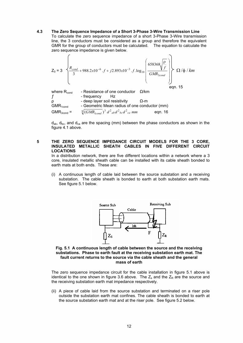
INSULATED METALLIC SHEATH CABLES IN FIVE DIFFERENT CIRCUIT LOCATIONS In a distribution network, there are five different locations within a network where a 3 core, insulated metallic sheath cable can be installed with its cable sheath bonded to earth mats at both ends. These are: (i) A continuous length of cable laid between the source substation and a receiving substation. The cable sheath is bonded to earth at both substation earth mats. See figure 5.1 below.

The zero sequence impedance circuit for the cable installation in figure 5.1 above is identical to the one shown in figure 3.6 above. The Zs and the ZR are the source and the receiving substation earth mat impedance respectively. (ii) A piece of cable laid from the source substation and terminated on a riser pole

outside the substation earth mat confines. The cable sheath is bonded to earth at the source substation earth mat and at the riser pole. See figure 5.2 below.

Fig. 5.1 A continuous length of cable between the source and the receiving substations. Phase to earth fault at the receiving substation earth mat. The

fault current returns to the source via the cable sheath and the general mass of earth

13

Figure 5.2 A cable and a line combination between the source and the receiving

substations. Phase to earth fault at the receiving substation earth mat. The fault current returns to the source via the general mass of earth and the cable

sheath

The zero sequence impedance circuit for the cable installation as shown in figure 5.2 above is shown in figure 5.3 below. RCE is the cable sheath bonding electrode resistance.

Figure 5.3 The zero sequence impedance circuit for the cable and line

combination shown in figure 5.2 above

(iii) A piece of cable laid from the riser pole (out side the confines of the receiving

substation earth mat) and terminated at the receiving substation. The cable sheath is bonded to earth at the riser pole and at the receiving substation earth mat. See figure 5.4 below.

Figure 5.4 A line and cable combination between the source and the receiving substations. Phase to earth fault at the receiving substation earth mat. The

fault current returns to the source via the cable sheath and the general mass of earth

14

The zero sequence impedance for the cable installation in figure 5.4 above is shown in figure 5.5 below.

Figure 5.5 The zero sequence impedance circuit for the line and the cable


(iv) A length of cable laid from the source substation to a riser pole and from another riser pole to the receiving substation with a line in between. Both ends of both cable sheaths are bonded to earth. See figure 5.6 below.

Figure 5.6 A cable, line and cable combination between the source and the receiving substations. Phase to earth fault at the receiving substation earth mat.

The fault current returns to the source via both cable sheaths and the general mass of earth


Figure 5.7 The zero sequence impedance circuit for a cable, line and cable


(v) A piece of cable laid from a riser pole to another riser pole, between the source substation and the receiving substation. See figure 5.8 below.

15

Figure 5.8 A line, cable, and line combination between the source and the receiving substations. Phase to earth fault at the receiving substation earth

mat. The fault current returns to the source via both the general mass of earth and the cable sheath


Figure 5.9 The zero sequence impedance circuit for a line, a cable and a line combination shown in figure 5.9 above

6 VALIDATION OF THE CABLE POSITIVE AND ZERO SEQUENCE MODELS

A separate study was carried out for a hypothetical cable to compare results from models developed here with results obtained using a very sophisticated cable model (Alternate Transients Program model) to ensure that these models were appropriate and correct for studying EPR and current splits in the cable network. The Alternate Transients Program (ATP) is a very powerful and sophisticated computer software program developed to study electromagnetic transients in an electrical network. In addition to performing transient simulations for a given network, it also calculates parameters for cables, lines, transformers, etc. The parameters are calculated using very accurate models for cables, lines and other equipment. The ATP not only calculates the series self and mutual impedance but also calculates the shunt (capacitance) admittance for cables and lines of any given configuration. It can be seen from the following figures 6.1 and table 6.1 that for the hypothetical cable, as the source voltage increases, the influence of the shunt admittance on the fault current splits and therefore the difference in results between the two models becomes noticeable. However, if the shunt admittance was neglected in the ATP model, the results becomes comparable. This shows that models presented in this paper are accurate for the type of analysis being performed. The ATP cable model parameter calculations are very difficult to perform without a computer. In contrast the models in this paper can be readily and easily used with a very basic scientific calculator.

16

Figure 6.1 Comparison of models for a hypothetical cable - fault current splits

Source Voltage 415V Current (A) A to B D to

earth D to C D to E E to

earth ATP Model Including Shunt Capacitance

36.513 +j153.72

0.014-j2.37 56.65 - j137.3

-20.16 - j13.84

-31.22 - j13.76

ATP Model Excluding Shunt Capacitance

36.202 j152.19

0.32-j1.67 56.014 - j136.55

-20.14 - j13.97

-20.14 - j13.97

Model Developed in this paper

34.737 - j151.247

032-j1.66 54.45 - j135.84

-20.02 - j13.74

-20.02 - j13.74

Source Voltage 11000V Current (A)

A to B D to



966.2 - j4067

0.37 - j62.81

1499 - j3639

-533.5 - j366

-826.17 j364


957.97 - j4027

8.64 - j44.29

1482 - j3613

-532.93 - j369

-532.9 - j369


920.75 - j4008

8.37 - j44.04

1443 - j3600

530.9 - k364.2

-530.9 - j364.2


A to B D to



2898.6 - j12203

1.11 - j188.46

4497.87 - j10917

-1600 - j1094

-2478 j1092


2873.9 - j12082

25.94 - j132.89

4446.77 - j10840

-1598.79 - j1109.10

-1598 - j1109


2762.3 -j12026

25.09 - j132.12

4329.79 -j10802

-1592.6 -j1092.17

-1592.6 -j1109


A to B D to



5797 - j24407

2.22 - j376

8995 - j21835

-3201 - j2196

-4957 - j2184


5747 - j24164

51.8 - j265.79

8893 - j21680

-3197 j2218

-3197 j2218


5524 - j24053

50.2 - j264.24

8659 - j21604

-3185 - j2185

-3185 - j2185

Table 6.1 Current split as calculated by different cable models. It can be seen

that if the shunt admittance was to be neglected from the ATP model, then model developed in this paper is accurate

17

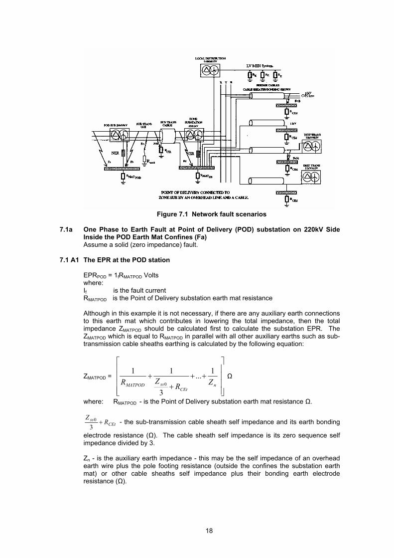
7 SYMMETRICAL COMPONENT MODEL FOR A PHASE TO EARTH FAULT IN A TYPICAL SUB-TRANSMISSION AND A DISTRIBUTION NETWORK The symmetrical components circuit models for a single phase-to-earth faults in a typical 33kV sub-transmission and a 11kV distribution network where a 220/33kV Point of Delivery substation is connected to a 33/11kV zone substation by an overhead line and a cable for the following five fault locations will be developed in this section (see Fig. 7.1). a) Fault at Point of Delivery (POD) substation on 220kV side inside POD earth mat

confines. b) Fault at POD substation on 33kV side inside POD earth mat confines c) Faults on a 33kV sub-transmission overhead line to zone substation, outside POD

and zone substation earth mat confines. d) Fault on a 33kV sub-transmission cable to zone substation, inside zone substation

earth mat confines. e) Fault on a 11kV feeder from zone substation outside zone sub-earth mat confines

- at a distribution substation earth mat. 7.1 Analysis of a Typical Sub-Transmission and Distribution Network

Point of Delivery substation (POD) connected to a Zone substation by a 33kV sub-transmission 3-phase 3-wire overhead line and a 3 core cable with an insulated metallic sheath. The Zone substation is connected to a 11,000/415V distribution substations by a 11kV 3 core cables with insulated metallic sheaths. In the following analysis, unless otherwise stated, it has been assumed that the cable sheath is insulated from the surrounding earth and both terminal ends are solidly bonded to the earth of known impedance. The figure 7.1 below shows the fault scenarios for this case.

18

Figure 7.1 Network fault scenarios

7.1a One Phase to Earth Fault at Point of Delivery (POD) substation on 220kV Side

Inside the POD Earth Mat Confines (Fa) Assume a solid (zero impedance) fault. 7.1 A1 The EPR at the POD station EPRPOD = 1fRMATPOD Volts where: If is the fault current RMATPOD is the Point of Delivery substation earth mat resistance Although in this example it is not necessary, if there are any auxiliary earth connections

to this earth mat which contributes in lowering the total impedance, then the total impedance ZMATPOD should be calculated first to calculate the substation EPR. The ZMATPOD which is equal to RMATPOD in parallel with all other auxiliary earths such as sub-transmission cable sheaths earthing is calculated by the following equation:

ZMATPOD =

+++

+n

CEtssMATPOD ZRZR

1...

3

110

Ω

where: RMATPOD - is the Point of Delivery substation earth mat resistance Ω.

CEtss RZ

+3

0 - the sub-transmission cable sheath self impedance and its earth bonding

electrode resistance (Ω). The cable sheath self impedance is its zero sequence self impedance divided by 3. Zn - is the auxiliary earth impedance - this may be the self impedance of an overhead earth wire plus the pole footing resistance (outside the confines the substation earth mat) or other cable sheaths self impedance plus their bonding earth electrode resistance (Ω).

19

7.1B One Phase to Earth Fault at Point of Delivery (POD) substation on 33kV Side Inside the POD Earth Mat Confines (Fb)

Assume a solid (zero impedance) fault to the earth mat.

For such a fault on the earth mat, no current will flow through the earth mat to the general mass of earth, therefore the Earth Potential Rise (EPR) of the station earth mat (RMATPOD) is equal to zero.

7.1C One Phase to Earth Fault On the 33kV Overhead Feeder to Zone Substation outside the POD Earth Mat Confines.

Assume a solid (zero impedance) fault. 7.1 C1 Fault at the 33kV Sub-transmission line pole Fci) With reference to figure 7.1 and 7.3. 7.1 C1.1 The Earth Potential Rise (EPR) of the sub-transmission pole EPRpole = 3I0RearthV I0 - zero sequence current. A Rearth - the resistance of the pole with respect to a remote earth Ω 7.1 C1.2 The EPR at the POD station EPRPOD = 3I0RMATPOD V I0 - zero sequence current. A RMATPOD - the resistance of the POD earth mat Ω

7.1 C2 Fault at the sub-transmission cable to overhead line termination joint (Fcii) Assume a solid (zero impedance) fault. With reference to figures 7.1 and 7.4:

20

For this particular type of fault, the zero sequence fault current will split between the cable sheath bonding earth electrode and the cable sheath. The zero sequence current flowing through the sheath will further split between the zone substation earth mat, 11kV feeder cable sheaths and the connected LV MEN system.

The EPR due to this fault will be transferred to the zone substation earth mat, the

distribution substation earth mats, and the LV MEN connected to these distribution substations.

7.1 C2.1 The Earth Potential Rise (EPR) of the sub-transmission cable sheath bonding electrode EPRRCEt = 3IgoRCEt V Igo - zero sequence current returning to the source through this electrode and

the general mass of earth. A RCEt - the resistance of the sub-transmission cable sheath bonding electrode Ω 7.1 C2.2 The EPR at the POD station EPRPOD = 3I0ZMATPOD V I0 - zero sequence current A RMATPOD - the resistance of the POD earth mat Ω 7.1 C2.3 The Transferred EPR to the Zone substation earthing system EPRzs = 3Ish0 ZMATseq V Ish0 - zero sequence current returning to the source via the sub-transmission

cable and the zone substation earthing system. A ZMATZSeq - the zone substation earthing system impedance (Ω). It is the zone

substation earthing system impedance measured with respect to a remote earth. The measurement should include the influence of the connected MEN system and the auxiliary earthing (e.g. cable sheaths bonded to earth

21

outside the substation earth mat) which contribute to this earthing system. The influence of the connected MEN system and the cable sheaths to the earth mat can be estimated by the following equations. From these equations, TEPR to remote points can also be assessed.

ZMATZSeq m - number of 11kV distribution cable sheaths connected to the zone substation

earth mat ZMATZS - the impedance of the earth mat with respect to the remote earth. This value

should preferably be obtained before installation of the 11kV cables and the LV MEN Ω Zss0d - the zero sequence self impedance of the 11kV distribution feeder cable

sheath Ω RCEd - the Distribution substation earthing system resistance measured with

respect to a remote earth (Ω). This value may include the impedance of the MEN system connected to this distribution substation earth mat.

ZMEN - the impedance of the MEN connected to the zone substation earth mat.

This value can be approximated by the following equation Ω

ZMEN = Ω

∑=

n

i nR1

11

Rn - customer earth electrode resistance Ω Note that the self impedance of the neutral conductor has been omitted from the above

equation. If the impedance of the neutral conductor is required in the above calculation, then a ladder network equation should be used to calculate the ZMEN.

7.1 C2.4 The Transferred EPR to the distribution substation earthing system With reference to figures 7.1 and 7.5:

Figure 7.5 In this figure, the circuit diagram of the transferred EPR

through cable sheath is shown. All impedance are in ohms

Ω

+

++∑

= MENCEdi

diss

m

iMATZS ZRZZ

1

3

11

1

01

22

The transferred EPR at a distribution substation is calculated by the following equation:

TEPRDS = EPRZS VR

ZR

CEddss

CEd

+3

0

where: RCEd - a Distribution substation earthing system resistance measured with respect

to a remote earth Ω Zss0d - the zero sequence self impedance of a 11kV distribution cable sheath Ω 7.1D One Phase to Earth Fault On the Feeder to Zone Substation Inside the Zone

Substation Earth Mat Confines (Fd) Assume a solid (zero impedance) fault to the earth mat With reference to figures 7.1 and 7.6:

7.1 D1 The Earth Potential Rise (EPR) of the POD station earth mat (R(MATPOD) is equal to EPRPOD = 3I0 RMATPOD V where: I0 - the zero sequence current A 7.1 D2 The Earth potential Rise (EPR) of the Zone substation (ZS) earth mat (ZMATZSeq) is

equal to EPRZS = 3IgoZMATZSeq V Igo - the zero sequence current returning to the source via zone substation

earthing system and the general mass of earth A

23

ZMATZSeq - the zone substation equivalent earthing system impedance (Ω). It was described in detail in section 7.1 C2.2 above.

7.1 D3 The Earth Potential Rise (EPR) of the sub-transmission cable sheath bonding

electrode With reference to figures 7.1 and 7.4: EPRRCE t = 3Ish0 RCE t V Ish0 - zero sequence current returning to the source through the 33kV cable

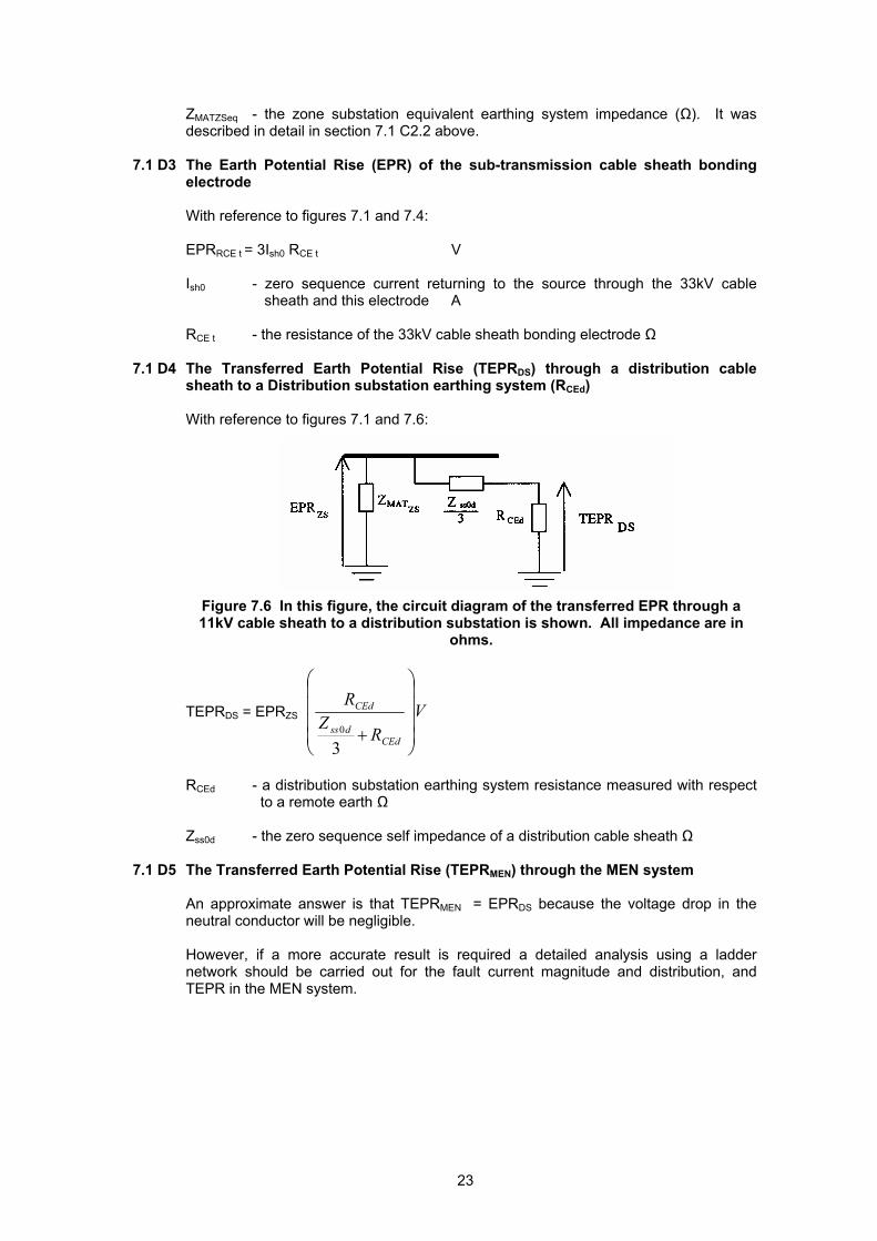
sheath and this electrode A RCE t - the resistance of the 33kV cable sheath bonding electrode Ω 7.1 D4 The Transferred Earth Potential Rise (TEPRDS) through a distribution cable

sheath to a Distribution substation earthing system (RCEd) With reference to figures 7.1 and 7.6:

Figure 7.6 In this figure, the circuit diagram of the transferred EPR through a 11kV cable sheath to a distribution substation is shown. All impedance are in

ohms.

TEPRDS = EPRZS VR

ZR

CEddss

CEd

+3

0

RCEd - a distribution substation earthing system resistance measured with respect

to a remote earth Ω Zss0d - the zero sequence self impedance of a distribution cable sheath Ω 7.1 D5 The Transferred Earth Potential Rise (TEPRMEN) through the MEN system An approximate answer is that TEPRMEN = EPRDS because the voltage drop in the

neutral conductor will be negligible. However, if a more accurate result is required a detailed analysis using a ladder

network should be carried out for the fault current magnitude and distribution, and TEPR in the MEN system.

24

7.1 E One Phase to Earth Fault on a (11kV) Cable Feeder at a Distribution Substation (Fe)

Assume a solid (zero impedance) fault. With reference to figures 7.1 and 7.7:

7.1 E1 The EPR at the Distribution Substation EPRDS = 3Igo RCEd V Igo - zero sequence current returning through the Distribution substation earth

mat and the general mass of earth A RCEd - the Distribution substation earthing system resistance measured with

respect to a remote earth. It includes the MEN system resistance Ω 7.1 E2 The EPR at the Zone Substation With reference to the figure 7.7 EPRZS = 3Igo ZMATzseqd V Igo - zero sequence current returning through the Distribution substation earth

mat A ZMATzseqd - the zone substation total earthing system impedance (earth mat resistance

in parallel with other distribution cable sheath bonding earth electrode resistance etc) measured with respect to a remote earth Ω. This impedance is different from ZMATzseq because it does not take into consideration the self impedance of the faulted cable sheath and its bonding earth electrode resistance.

Figure 7.7 The sequence network for fault Feii. In this figure, Zsource and 3ZNER are 11kv system impedance

25

7.1 E3 The Transferred Earth Potential Rise (TEPRMEN) from the Distribution Substation to the MEN system

An approximate answer is that TEPRMEN = EPRDS because the voltage drop in the

neutral conductor will be negligible. However, if a more accurate result is required a detailed analysis using a ladder

network should be carried out for the fault current magnitude and distribution, and TEPR in the MEN system.

8 A NUMERICAL EXAMPLE A complete set of calculations illustrating the use of the models developed in Section 7

of this paper were performed for typical phase to earth fault scenarios. These calculations are annexed in appendix B.

The scenarios studied are for the network discussed in Section 7, where a POD

substation was connected to a zone substation by an overhead line and a cable for the following five single phase to earth fault locations:

a) Fault at Point of Delivery (POD) substation on 220kV side inside POD earth mat

confines (Fa). b) Fault at POD substation on 33kV side inside POD earth mat confines (Fb). c) Faults on a 33kV sub-transmission overhead line from a POD substation to a

zone substation, outside the POD and zone substation earth mat confines (Fci and Fcii).

d) Fault on a 33kV sub-transmission cable from a POD substation to a zone substation, inside zone substation earth mat confines (Fd).

e) Fault on a 11kV feeder from zone substation to a distribution substation earth mat (Fe).

Table 8.1 below summarises EPR and the TEPR results for all of these faults at the various fault locations in the network shown in figure 7.1.

Description of Earth Mats The EPR and the TEPR for the following faults (Volts)

Fa Fb Fci Fcii Fd Fe 1 Point of Delivery substation 7446 0 371 5351 4250 N/A 2 At 33kV Pole N/A N/A 18,545 N/A N/A N/A 3 Sub-transmission cable

Sheath bonding electrode

N/A

N/A

N/A

3816

6470 Reader to Calculate

4 Zone substation earth mat N/A N/A N/A 868 694 52 5 Distribution substation (1)

earth mat. No MEN connected at this substation at this stage

N/A

N/A

N/A

814

662

3102

6 Distribution substation earth Mat (2) with MEN connected At this substation

N/A

N/A

N/A

318

217

Reader to calculate

Table 8.1 Summary of EPR calculation results from Appendix B

The graphs in figures 8.1 to 8.6 below show the influence of the resistance of the various earth

mats on EPR in the 33kV and the 11kV networks modelled.

26

Resistance of Pole Earth (Ohm) EPR at Pole earth

EPR at POD substation Figure 8.1 EPR at the Pole earth and the POD substation earth mat due

to a 33kV Ph-E fault at a pole midway along the line F(ci)

Figure 8.1 above shows the EPR at the pole and the POD substation for different pole earth resistance values. It can be seen that increasing the pole earth resistance causes reduced EPR at the POD substation. It also shows that EPR at the pole will be very high if the POD substation earth mat resistance is very low compared to the pole earth resistance. The EPR at the pole earth can be reduced by installing a NER at the source substation as shown in figure 8.2 below.

Resistance of Pole Earth (Ohm) EPR at Pole earth 20 Ohm NER EPR at POD substation 20 Ohm NER Figure 8.2 EPR at the Pole earth and the POD substation due to a 33kV Ph-E fault

at a pole midway along the line (F(ci)). A 20 Ohm NER is connected at the source substation

In figure 8.3 below, the influence of the 33kV cable sheath bonding electrode

resistance on the EPR at the POD substation, zone substation and 11kV distribution substation is shown. From this figure, it is observed that after certain maximum threshold value of the electrode resistance, an additional increase in the cable sheath electrode resistance has an insignificant effect on the EPR at the various locations in the 33kV and 11kV networks.

27

Figure 8.3 EPR due to a 33kV Ph-E fault at the 33kV cable to line termination joint (Fcii) for increasing value of the cable sheath bonding electrode

resistance. The EPR at the sheath bonding electrode, POD substation, zone substation and distribution substation earth mats are shown

From figure 8.3, it can be observed that (for 1 Ohm POD substation earth mat resistance) the POD substation EPR is always higher than the EPR in the rest of the network for all values of the cable sheath bonding electrode resistance. The benefit of using a 20 Ohm NER for reducing EPR for the above fault scenario is shown in figure 8.4 below.

From figure 8.4 above, it can be seen that the EPR at the POD reduces from 5,300V to 850V with a 20 Ohm NER. Likewise, EPR in the rest of 33kV and 11kV networks are reduced. Figures 8.5a and b below show EPR in the 33kV and the 11kV networks due to a 33kV fault at the zone substation (Fd) for various zone substation earth mat resistance values.

28

From figures 8.5a and b above, it can be observed that the EPR at the 33kV cable sheath bonding electrode (25 Ohm) and the POD substation earth mat (1 Ohm) is relatively very high for this particular fault for various values of the zone substation earth mat resistance. From 8.5b it can be seen that there is very little increase in the zone substation EPR for the earth mat resistance values greater than 1 Ohm.

Figures 8.6a, b and c below show the EPR in the 33kV and 11kV network due to a 11kV fault (Fe) at a distribution substation without a MEN connected to its earth mat.

Figure 8.6 c Figure 8.6 EPR due to a 11kV Ph-E fault at a distribution substation (Fd) without

MEN connection, for increasing values of the distribution substation earth mat resistance. The EPR at the 33kV cable sheath bonding electrode, zone substation and distribution substation earth mats are shown.

Figure 8.5a Figure 8.5b Figure 8.5 EPR due to a 33kV Ph-E fault at the zone substation (Fd) for increasing value of the zone substation earth mat resistance. The EPR at the 33kV cable sheath bonding electrode, POD substation, zone substation and a distribution substation earth mats are shown.

29

From figures 8.6a, b and c, it can be seen that for distribution substation earth mat resistances greater than 10 Ohm, there is very little influence on the magnitude of EPR in the 33kV and 11kV networks. Once again, the benefit of a 20 Ohm NER in reducing EPR can be seen in figure 8.6b. For very low values of the distribution substation earth mat resistance, the EPR at 33kV cable sheath bonding electrode and the zone substation earth mat will be relatively high.

In figures 8.3 to 8.6, it was shown that there exists a maximum threshold earth mat

resistance for a given earth mat in an interconnected earthing system, beyond which there is insignificant increase in the EPR. This is a very important observation since reducing one substation earth mat’s resistance to reduce its EPR, can cause an increase in EPR in the other parts of the network.

It was also shown that if the receiving substation earthing system impedance was lower

than the source substation, then the source substation may have highest EPR in that network. Relatively high earthing system resistance at the receiving substation means lower EPR at the source substation.

CONCLUSIONS In this paper, equations for calculating positive and zero sequence impedances for an overhead line and an underground three core, insulated metallic sheath covered cable are given. Appropriate symmetrical component circuit models were developed to calculate the phase to earth fault current and fault current split between the cable sheath and the earth mat.

When using the symmetrical components method of analysis of unbalanced faults in cable networks, the zero sequence impedance model of the 3-core, insulated metallic sheath cable is important for calculating EPR. Cables installed in different locations in a network (e.g. all cable, cable-line, line-cable, cable-line-cable and line-cable-line) will have different zero sequence impedance circuit models. Since EPR is caused by the zero sequence current, it is important to use the correct zero sequence impedance model.

The fault current splits calculated by models developed in this paper were checked for their validity against the more sophisticated Alternate Transients Program (ATP) models. The results of this comparison show that the models presented in this paper are sufficiently accurate for current split calculations.

Numerical examples are given to illustrate the application of the models for calculating fault current splits and the earth potential rise for various fault locations in a typical sub-transmission and distribution network.

The calculations show that even though 96% of the total fault current in the 11kV cable network with bonded cable sheaths returns to the source via the sheath, the EPR for 10 Ohms earthing system resistance can be as high as 3100 Volts (i.e. 49% of the system voltage). The calculations show that the benefits of cable sheath bonding on EPR levels are mixed. For the case of the 11kV cable sheath bonded to both the 33/11kV zone substation and 11kV/415V distribution substation earthing systems, the effects of cable sheath bonding are: (i) For an 11kV ph - E fault at the distribution substation, the EPR at both the zone and distribution substations will be low. (ii) For a 33kV ph-E fault at the zone substation, the resultant EPR at the zone substation will be reduced, but at the COST of transferring almost all this EPR to the distribution substation earthing system (which would otherwise have had no EPR). However, in an extensively MEN system, this EPR level will be insignificant, and bonding of cable sheaths will reduce it even further. A neutral earthing resistor (NER) will act as a voltage divider in the fault circuit and can substantially reduce the EPRs in the network.

30

The sequence impedance parameters (for lines and cables) and fault circuit models developed in this paper can also be used to calculate parameters required by power system analysis software such at PTI’s PSS/U. REFERENCES 1. Wagner C.F. and Evans R.D. “SYMMETRICAL COMPONENTS AS APPLIED TO THE

ANALYSIS OF UNBALANCED ELECTRICAL CIRCUITS” 2. Skilling H.H. “ELECTRIC TRANSMISSION LINES Distributed Constants, Theory and

Applications”.

ACKNOWLEDGEMENTS The author wishes to acknowledge the support from NZCCPTS and the financial assistance received from the Standards Australia for travel, accommodation and meals to present this paper in Melbourne. The author also wishes to acknowledge the technical advice received from Mr. T.L. Scott (General Manager Network Services) and Mr. Stephen Hirsch (Planning Engineer - Network) of Southpower, Mr. Alan Marshall and Dr Gordon Cameron of Telecom NZ Ltd., Dr. Don Geddey and Stephen Boroczky of Transgrid, Sydney, Patrick Pearl SEQEB Brisbane, and Dr. Maria Kobe of Mercury Energy, Auckland New Zealand, on the subject of cable modelling and distribution system earthing design. Their timely advice and motivation has made this paper a reality.

1

APPENDIX A

CALCULATIONS OF GMR, POSITIVE AND ZERO SEQUENCE LINE AND CABLE PARAMETERS

A.1 Calculation of Geometric Mean Radius of ASCR Conductor The GMR of ASCR conductors are calculated by considering positions of Aluminium strands in the conductor. It is assumed that no current flows in the steel strands and therefore are omitted from the calculation. For illustration, the GMR calculation for the DOG (Al - 6/4.72 mm and Fe - 7/1.57 mm) conductor is given below. The diameter of 7/1.57 mm strands is equal to 4.72 mm

GMR = 36 61212641

)4()32()2()( rrrre−

GMR = 2.3038r

GMR = (0.768)(7.1mm)

GMR = 5.453 mm A.2 Calculation of the Line Parameters 33kV Line - Physical dimensions Conductor type = DOG (6/4.72 Al & 7/1.57 Steel strands) Resistance of the Conductor @ 20 deg C (ohms/km) R := 0.2722 Approximate overall diameter (mm) d := 14.2 Radius of the conductor mm a “=

2d

Spacing between lines (mm) dab := 1090 dbc := 880 dac := 1970 Deep layer soil resistivity (ohm-m) ρ := 200 frequency (Hz) f := 50

GMR := a0.768 GMD := [(dab.dbc.dac) 31

] GMR3cond := [GMR3.dab2.dbc2.dac2) 91

] GMR = 5.4528 GMD = 1236.3036 GMR3cond = 202.748

2

Positive sequence Impedance (ohms/km)

Z1 = R + j .

−GMRGMDf log..10.893.2 3 Z1 = 0.2722 + 0.3407j

Zero sequence Impedance (ohms/km)

Z0 := 3.

++ −−

condGMRf

fjfR3

.658368log..10.893.2..10.2.988

336

ρ

Z0 = 0.4204 + 1.6545j

A.3 Calculation of the Cable Parameters 33kV PILCA cable. Physical dimensions Conductor type = 150 AL (37 strands) assume round conductor Resistance of the Conductor @ 20 deg C (ohms/km) R :=0.2060 Radius of the conductor (mm) a := 6.764 Spacing between conductors (mm) S := 27.76 Resistivity of the sheath (ohm-m) ρsh := 21.4.10 -8 Inside radius of the sheath (mm) ri := 30.36 Outside radius of the sheath (mm) ro := 33.09 Soil resistivity (ohm-m) ρ := 200 frequency (Hz) f := 50

GMR :=a.0.768 GMRsh := 2riro+ dsh := GMRsh GMR3cond := [(GMR.S2) 3

1 ] GMR = 5.1948 GMRsh = 31.725 dsh = 31.725 GMR3cond = 15.8782

Rsh := ( )2.2

9

.10.riro

sh−π

ρ Rsh = 0.3933

Positive sequence impedance (ohms/km)

Z 1 := R + j .

−GMRSf log..10.893.2 3 Z1 = 0.206 + 0.1053j

Zero sequence Self Impedance of the conductor (ohms/km)

Zsc0 := 3.

++ −−

condGMRf

fjfR3

.658368log..10.893.2..10.2.988

336

ρ

Zsc0 = 0.3542 + 2.1345j

Zero sequence Self Impedance of the sheath (ohms/km)

Zss0 :=3.

++ −−

condGMRf

fjfRsh3

.658368log..10.893.2..10.2.988 36

ρ

Zss0 = 1.328 + 2.004j

3

Zero impedance Mutual Impedance (ohms/km)

Zmcs0 := 3.

+ −−

dshf

fjf

ρ.658368log..10.893.2..10.2.988 36 Zmcs0 = 0.1482 + 2.004j

Zero sequence impedance of the cable for the Model (ohms/km)

Zcond0 :=Zsc0 - Zmcs0 Zcond0 = 0.206 + 0.1304j

Rsh0 := Zss0 -Zmcs0 Rsh0 = 1.1798

Zg0 := Zmcs0 Zg0 = 0.1482 + 2.004j

4

1

APPENDIX B

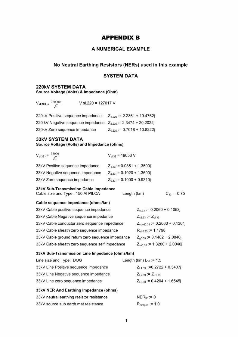
A NUMERICAL EXAMPLE

No Neutral Earthing Resistors (NERs) used in this example

SYSTEM DATA

220kV SYSTEM DATA Source Voltage (Volts) & Impedance (Ohm) Vsl.220 :=

3220000

V sl.220 = 127017 V

220kV Positive sequence impedance Z1.220 := 2.2361 + 19.4762j

220 kV Negative sequence impedance Z2.220 := 2.3474 + 20.2022j

220kV Zero sequence impedance Z0.220 := 0.7018 + 10.8222j 33kV SYSTEM DATA Source Voltage (Volts) and Impedance (ohms) Vsl.33 :=

333000 Vsl.33 = 19053 V


33kV Negative sequence impedance Z2.33 := 0.1020 + 1.3600j

33kV Zero sequence impedance Z0.33 := 0.1000 + 0.9310j 33kV Sub-Transmission Cable Impedance Cable size and Type : 150 Al PILCA Length (km) C33 := 0.75 Cable sequence impedance (ohms/km) 33kV Cable positive sequence impedance Zcl.33 := 0.2060 + 0.1053j

33kV Cable Negative sequence impedance Zc2.33 := Zcl.33

33kV Cable conductor zero sequence impedance Zcond0.33 := 0.2060 + 0.1304j

33kV Cable sheath zero sequence impedance Rsh0.33 := 1.1798

33kV Cable ground return zero sequence impedance Zg0.33 := 0.1482 + 2.0040j

33kV Cable sheath zero sequence self impedance Zss0.33 := 1.3280 + 2.0040j 33kV Sub-Transmission Line Impedance (ohms/km) Line size and Type: DOG Length (km) L33 := 1.5

33kV Line Positive sequence impedance ZL1.33 :=0.2722 + 0.3407j

33kV Line Negative sequence impedance ZL2.33 := ZL1.33

33kV Line zero sequence impedance ZL0.33 := 0.4204 + 1.6545j 33kV NER And Earthing Impedance (ohms) 33kV neutral earthing resistor resistance NER33 := 0

33kV source sub earth mat resistance Rmatpod := 1.0

2

33kV Cable sheath bonding earth electrode resistance RCE t := 25

33kV line to earth fault resistance (e.g. at a pole) Rearth := 50 11kV SYSTEM DATA Source Voltage (volts) & Impedance (ohms) Vsl.11:=

311000 Vs1.11 - 6351 V


11kV Negative sequence impedance Z2.11 := Z1.11

11kV Zero sequence impedance Z0.11 := 0.04261 + 0.4261j 11kV Distribution Cable Impedance 1. Cable size and Type : 300 Al PILCA Length (km) L1 := 0.75

Cable sequence impedance (ohms/km) 11kV Cable Positive sequence impedance Z c1.1 := 0.1086 + 0.0711j

11kV Cable Negative sequence impedance Zc2.1 := Z c1.1

11kV Cable conductor zero sequence impedance Z cond0.1 := 0.1001 + 0.1049j



11kV Cable sheath zero sequence self impedance Zss0.1 := 1.9020 + 2.0337j

2. Cable size and Type : 300 Al PILCA Length (km) L2 := 1.25

Cable sequence impedance (ohms/km) 11kV Cable Positive sequence impedance Zcl.2 := 0.1086 + 0.0711j

11kV Cable Negative sequence impedance Zc2.2 := Zc1.1



11kV Cable ground return zero sequence impedance Z g0.2 := 0.1480 + 2.0337j

11kV Cable sheath zero sequence self impedance Zss0.2 := 1.9020 + 2.0337j 3. Cable size and Type : 300 A1 PILCA Length (km) L3 ;= 0.25

Cable sequence impedance (ohms/km) 11kV Cable Positive sequence impedance Zc1.3 := 0.1086 + 0.0711j

11kV Cable Negative sequence impedance Z c2.3 := Zc1.1


11kV Cable sheath zero sequence impedance R sh0.3 := 1.754


11kV Cable sheath zero sequence self impedance Zss0.3 := 1.9020 + 2.0337j

3

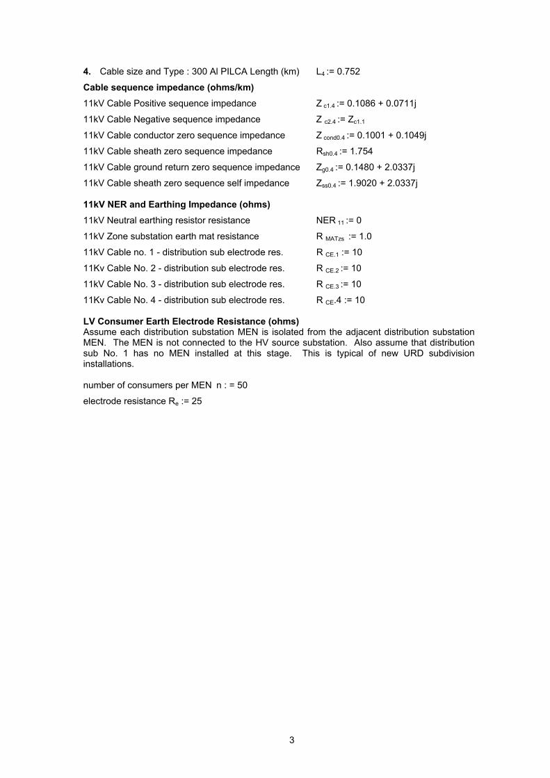
4. Cable size and Type : 300 Al PILCA Length (km) L4 := 0.752

Cable sequence impedance (ohms/km) 11kV Cable Positive sequence impedance Z c1.4 := 0.1086 + 0.0711j

11kV Cable Negative sequence impedance Z c2.4 := Zc1.1




11kV Cable sheath zero sequence self impedance Zss0.4 := 1.9020 + 2.0337j 11kV NER and Earthing Impedance (ohms) 11kV Neutral earthing resistor resistance NER 11 := 0

11kV Zone substation earth mat resistance R MATzs := 1.0

11kV Cable no. 1 - distribution sub electrode res. R CE.1 := 10

11Kv Cable No. 2 - distribution sub electrode res. R CE.2 := 10

11kV Cable No. 3 - distribution sub electrode res. R CE.3 := 10

11Kv Cable No. 4 - distribution sub electrode res. R CE.4 := 10 LV Consumer Earth Electrode Resistance (ohms) Assume each distribution substation MEN is isolated from the adjacent distribution substation MEN. The MEN is not connected to the HV source substation. Also assume that distribution sub No. 1 has no MEN installed at this stage. This is typical of new URD subdivision installations. number of consumers per MEN n : = 50

electrode resistance Re := 25

4

CALCULATIONS 7A1 The EPR at the POD Station (Fault Fa) Refer fig. 7.1 in the text Zero sequence fault current

I0.220 :=

MATPODRZZZsV

.3220.0220.2220.1

220.1+++

I 0.22 := 401.8 - 2449.2J A

220.0I = 2482 A

Fault current (Amps)

If 220 := 3I0.220

If 220 = 1205.5 - 7347.7J A

220If = 7445.9 A

EPRPOD := If 22o .RMATPOD

PODEPR = 7445.9 Ohm

7C1 Fault at the sub-transmission line pole (midway of the line) (Fci). With reference to figure 7.3

Sequence network impedance (ohms)

Zpos.33 :Z1.33 ZL1.33 . 233L Zpos.33 = 0.2893 + 1.6055j

Zneg.33 := Z2.33 + ZL2.33 . 233L Zneg.33 + 0.3061 + 1.6155j

Zzero.33 := Z0.33 + ZL0.33 . 233L + 3.4earth + 3.RMATPOD zzero.33 = 153.4153 + 2.1719j

Zero sequence fault current (Amps)

I0:= 3333.33.33.

33.1

.3 NERZZV

zeronegpos

s

+++

I0 = 123.6 - 4.3J A

0I = 123.6335 A

Fault current (Amps)

If = 3.I0

If = 370.7 - 13j A

If = 370.9 A

7C1.1 The EPR of the sub-transmission line pole (Rearth) (Volts) EPRRearth := 3.I0 .Rearth

arthEPRRe = 18545 V

5

2C1.2 The EPR at the POD station (Volts) EPRPOD := 3.I0 .RMATPOD

PODEPR = 370.9 V

7C2 Fault on the sub-transmission line to cable termination joint (Fcii). With reference to figure 7.4

Sequence network impedance (Ohms)

Zpos.33 := Z1.33 = ZL2.33 .L33 Zpos.33 = 0.4934 + 1.8611j

Zneg.33 := Z2. + ZL2.33 .L33 Zneg.33 = 0.51-03 + 1.8711j

Calculate ZMATzseq (Ohms)

Zss - total self impedance of the 11kV feeder cables including their sheath bonding electrode resistance.

ZMEN :=

eRn 1..

1 ZMEN = 0.5

The equivalent impedance of the distribution sub earthing : electrodes + MEN. MEN at distribution sub No. 1 not installed at this stage.

ZdsMEN.1 := RCE.1 ZdsMEN.2

1

2.

11−

+

MENCE ZR

ZdsMEN 3:= 1

3.

11−

+

MENCE ZR ZdsMEN.4 :=

1

4.

11−

+

MENCE ZR

Zss

:=

1

4.44.033.0

2.22.0

1.11.0

3.

1

3.

1

3.

1

3.

1

−

++

++

++

+ dsMENss

dsMENSS

dsMENss

dsMENss Z

LZZ

LZZ

LZZ

LZ

Zss = 0.2926 + 0.1198j

ZMATzseq := 1

111−

++

MENssMATzs ZZR ZMATzseq = 0.1621 + 0.0328j

Zsero.33 := Z0.33 + ZL0.33 .L33 + 1

3333.0 .3.1

.31

−

++

MATzseqsstCE ZCZR + 3.RMATPOD

zZERO.33 = 5.2164 + 4.9519J

6

Zero sequence fault current (Amps

I0 := 3333.33.33.

33.1

.3 NERZZZV

zeronegpos

s

+++

I0 = 1038.6 - 1450j A

0I = 1783.6 A

Fault current (Amps) If = 3.10

If = 3115.9 - 4350.1j A

fI = 5350.9 A

Zero sequence fault current returning through the cable sheath (Amps)

Ish0 := I0. MATzseqZtCE

tCE

ZCRR

ss.333..3

.3

33.0++

Ish0 = 988.3 - 1442.6j A

0shI = 1748.7 A

Zero sequence fault current returning through earth (Amps)

Ig0 :=I0 . MATzseqsstCE

MATzseqss

ZCZRZCZ

.3..3.3.

33.0

3333.0

++

+

Ig0 = 50.3 - 7.4j

0gI = 50.9

7C2.1 The Earth Potential Rise (EPR) of the sub-transmission cable sheath bonding electrode (RCEt) (Volts)

EPRRCE t = 3.1g0 .RCE t

EPRRCE t = 3775 - 555.9j V

RCEtEPR = 3815.7 V

7C2.2 The EPR at the POD station (Volts) EPRPOD := 3.I0 .RMATPOD

EPRPOD = 3115.9 - 4350.1j V

PODEPR = 5350.9

7C2.3 The Transferred EPR at the Zone substation (Volts) EPRzs := 3.Ish0 .ZMATzseq

EPRzs =622.4 - 604.4j

zsEPR = 867.6

7

7C2.4a The Transferred EPR at the distribution substation 1 (Volts)

TEPRDS.1 := EPRZS .

+ 1.

1.0

1.

3 DSmenSS

dsMEN

zzZ

TEPRDS.1 = 546.8 - 603.3j

1.dsTEPR = 814.2 V

7C2.4b The Transferred EPR at the distribution substation 2 (Volts)

TEPRDS.2 := EPRZS .

+ 2.

2.0

2.

3 dsMENss

dsMEN

ZZ

z

TEPRDS.2 = 79.1 - 307.6J

2.DSTEPR = 317.6 V

7D One phase to Earth fault on the 33kV sub-transmission feeder to Zone substation inside the zone Substation earth mat confines (Fd). With reference to figure 7.5

Sequence network impedance Zpos.33 := Z1.33 + ZL1.33 .L33 + Zcl.33 .C33 Zpos.33 = 0.6479 + 1.94j

Zneg.33 = Z2.33 +ZL2.33 .L33 + Zc2.33 .C33 Zneg.33 = 0.6648 + 1.95j

Zzero.33 := Z0.33 + ZL0.33 .L33 + Zcond0.33 .C33 + 1

3333.03333.0 ..3.31

.3.1

−

++

+ CZZRCR gMATzseqtCEsh

Zzero.33 = 1.966 + 8.0037j


I0 := 3333.33.33.

33.

.3.3 NERRZZZV

MATPODzeronegpos

sl

++++

I0 = 661.3 - 1252.8j A

0I = 1416.6 A

Fault current If := 3.I0

If = 1984 - 3758.3j A

fI = 4249.9 A

8

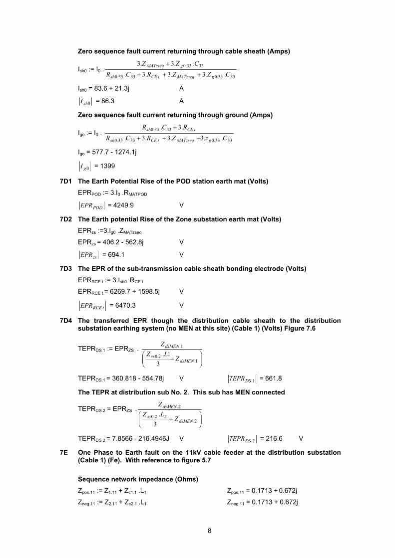
Zero sequence fault current returning through cable sheath (Amps)

Ish0 := I0 .3333.03333.0

3333.0

..3.3.3...3.3

CZZRCRCZZ

gMATzseqtCEsh

gMATzseq

+++

+

Ish0 = 83.6 + 21.3j A

0shI = 86.3 A

Zero sequence fault current returning through ground (Amps)

Igo := I0 . 3333.03333.0

3333.0

..3.3.3..3.

CzZRCRRCR

gMATzseqtCEsh

tCEsh

+++

+

Igo = 577.7 - 1274.1j

0gI = 1399

7D1 The Earth Potential Rise of the POD station earth mat (Volts) EPRPOD := 3.I0 .RMATPOD

PODEPR = 4249.9 V

7D2 The Earth potential Rise of the Zone substation earth mat (Volts) EPRzs :=3.Ig0 .ZMATzseq

EPRzs = 406.2 - 562.8j V

zsEPR = 694.1 V

7D3 The EPR of the sub-transmission cable sheath bonding electrode (Volts) EPRRCE t := 3.Ish0 .RCE t

EPRRCE t = 6269.7 + 1598.5j V

tRCEEPR = 6470.3 V

7D4 The transferred EPR though the distribution cable sheath to the distribution substation earthing system (no MEN at this site) (Cable 1) (Volts) Figure 7.6

TEPRDS.1 := EPRZS .

+ 1.

2.0

1.

31.

dsMENss

dsMEN

ZLZZ

TEPRDS.1 = 360.818 - 554.78j V 1.DSTEPR = 661.8

The TEPR at distribution sub No. 2. This sub has MEN connected

TEPRDS.2 = EPRZS .

+ 2.

22.0

2.

3.

dsMENss

dsMEN

ZLZZ

TEPRDS.2 = 7.8566 - 216.4946J V 2.DSTEPR = 216.6 V

7E One Phase to Earth fault on the 11kV cable feeder at the distribution substation (Cable 1) (Fe). With reference to figure 5.7

Sequence network impedance (Ohms) Zpos.11 := Z1.11 + Zc1.1 .L1 Zpos.11 = 0.1713 + 0.672j

Zneg.11 := Z2.11 + Zc2.1 .L1 Zneg.11 = 0.1713 + 0.672j

9

The bonded cable sheaths of the other three distribution substation also conducts ground return current to the source in parallel with the source sub earth mat. Zss is the equivalent impedance of 3 x 11kV cable sheaths + electrode + MEN and the 33kV cable sheath self impedance + RCE t .MEN of each distribution sub is assumed to have no metallic interconnection to the adjacent distribution sub MEN systems. It is also assumed that the distribution sub under investigation has no MEN system installed at this stage.

Zss := 1

33.04.

44.03..

33.02.

22.0

3

1

3.

1

3.

1

3.

1

−

++

++

++

+ tCEss

dsMENss

dsMENss

dsMENss R

ZZ

LZZ

LZZ

LZ

Zss = 0.2969 + 0.1235j

ZMATzseqd := 1

111−

++

MENssMATzs ZZR ZMATzseqd = 0.1636 + 0.0333j

Zzero.11 := Z0.11 + Zcond0.1 .L1 + 1

11.01.11.0 .3..31

.1

−

++

MATzseqdgCEsh ZLZRLR

Zzero.11 = 1.3791 + 0.5075j


I0 := 1111.11.11.

11.1

.3 NERZZZV

zeronegpos

s

+++

I0 = 1710.5 - 1839.6j A

0I = 2511.9 A

Fault current (Amps) If = 3.I0

If = 5131.4 - 5518.7j A

fI = 7535.7 A

Zero sequence fault current returning via 11kV cable sheath (Amps)

Ish0 := I0 .( )

( )MATzseqdgCEsh

MATzseqdgCE

ZLZRLRZZR

.3..3..33

11.01.11.0

1.01.

+++

++

Ish0 = 1644 - 1760.4j A

0shI = 2408.7 A

Percentage of total fault current returning via sheath

Ish (%) := 0

0

II sh . 100 (%)shI = 95.9

Zero sequence fault current returning via earth (Amps)

Ig0 := I0 ( )MATzseqdgCEsh

sh

ZLZRLRLR

.3..3..

11.01.11.0

11.0

+++

Ig0 = 66.5 - 79.2j A 0gI = 103.4 A

10

Percentage of total fault current returning via earth

Ig (%) := 0

0

II g .100 (%)gI = 4.1

7E1 The EPR at the Distribution substation (Volts) EPRds := 3.Ig0 .RCE.1

EPRds = 1994 - 2376.1j V

dsEPR = 3101.9 V

7E2 The EPR at the Zone substation EPRzs := 3.Ig0 .ZMATzseqd

EPRzs = 40.5 - 32.2j V

zsEPR = 51.8 V

Documents

FUNDAMENTALS OF CALCULATION OF EARTH … Sheath Bonding Application... · EARTH POTENTIAL RISE IN THE UNDERGROUND POWER DISTRIBUTION CABLE ... The calculation of sequence impedances