Embed Size (px)
Citation preview
Fundamentals of a SustainableU.S. Biofuels Policy
January 2010
Prepared by
The Energy Forum of the James A. Baker III Institute for Public Policyof Rice University
and
Rice University’s Department of Civil and Environmental Engineering
JAMES A. BAKER III INSTITUTE FOR PUBLIC POLICY
RICE UNIVERSITY
FUNDAMENTALS OF A
SUSTAINABLE U.S. BIOFUELS POLICY
PREPARED IN CONJUNCTION WITH AN ENERGY STUDY SPONSORED BY THE
JAMES A. BAKER III INSTITUTE FOR PUBLIC POLICY AND THE
RICE UNIVERSITY DEPARTMENT OF CIVIL AND ENVIRONMENTAL ENGINEERING
JANUARY 2010
Fundamentals of a Sustainable U.S. Biofuels Policy
2
THESE PAPERS WERE WRITTEN BY A RESEARCHER (OR RESEARCHERS) WHO PARTICIPATED IN A
BAKER INSTITUTE/RICE UNIVERSITY CEE RESEARCH PROJECT. WHEREVER FEASIBLE, THESE
PAPERS ARE REVIEWED BY OUTSIDE EXPERTS BEFORE THEY ARE RELEASED. HOWEVER, THE
RESEARCH AND VIEWS EXPRESSED IN THESE PAPERS ARE THOSE OF THE INDIVIDUAL
RESEARCHER(S), AND DO NOT NECESSARILY REPRESENT THE VIEWS OF THE JAMES A. BAKER
III INSTITUTE FOR PUBLIC POLICY OR THE RICE UNIVERSITY DEPARTMENT OF CIVIL AND
ENVIRONMENTAL ENGINEERING.
© 2010 BY THE JAMES A. BAKER III INSTITUTE FOR PUBLIC POLICY OF RICE UNIVERSITY
THIS MATERIAL MAY BE QUOTED OR REPRODUCED WITHOUT PRIOR PERMISSION,
PROVIDED APPROPRIATE CREDIT IS GIVEN TO THE AUTHOR AND
THE JAMES A. BAKER III INSTITUTE FOR PUBLIC POLICY.

Fundamentals of a Sustainable U.S. Biofuels Policy
3
ACKNOWLEDGMENTS
The James A. Baker III Institute for Public Policy and the Rice University
Department of Civil and Environmental Engineering would like to
thank Chevron Technology Ventures and the Institute for Energy
Economics of Japan for their generous support of this research.
Fundamentals of a Sustainable U.S. Biofuels Policy
4
ABOUT THE STUDY:
FUNDAMENTALS OF A
SUSTAINABLE U.S. BIOFUELS POLICY
The Baker Institute Energy Forum and Rice University’s Department of Civil and Environmental
Engineering have embarked on a two-year project examining the efficacy and impact of current U.S.
biofuels policy. Successful implementation of a sustainable biofuels program requires careful
analysis of the potential strengths and weaknesses of the current mandated program. Corporate
leaders are also in need of complete data to assess expanded industry participation in the biofuels
area.
The United States is investing billions of dollars each year in subsidies and tax breaks to domestic
ethanol producers in the hope that biofuels will become a major plank of an energy security and fuel
diversification program. Moreover, the investment has grown in recent years.
This study assesses the value of the expensive program and its potential to meet the goal of
enhancing energy security in an environmentally sustainable fashion. The policy research is designed
to identify the steps necessary to avoid unintended negative impacts on sustainable development and
the environment, including deleterious impacts on domestic agriculture, surface and ground water,
and overall air quality in the United States. It also addresses the daunting logistical and economic
challenges of expanding biofuels supplies into the U.S. fuel system and examines the costs and
benefits of different options.
STUDY AUTHORS
PEDRO ALVAREZ
JOEL G. BURKEN
JAMES D. COAN
MARCELO E. DIAS DE OLIVEIRA
ROSA DOMINGUEZ–FAUS
DIEGO E. GOMEZ
AMY MYERS JAFFE
KENNETH B. MEDLOCK III
SUSAN E. POWERS
RONALD SOLIGO
LAUREN A. SMULCER
Fundamentals of a Sustainable U.S. Biofuels Policy
5
ABOUT THE ENERGY FORUM AT THE
JAMES A. BAKER III INSTITUTE FOR PUBLIC POLICY
The Baker Institute Energy Forum is a multifaceted center that promotes original, forward-looking
discussion and research on the energy-related challenges facing our society in the 21st century. The
mission of the Energy Forum is to promote the development of informed and realistic public policy
choices in the energy area by educating policymakers and the public about important trends—both
regional and global—that shape the nature of global energy markets and influence the quantity and
security of vital supplies needed to fuel world economic growth and prosperity.
The forum is one of several major foreign policy programs at the James A. Baker III Institute for
Public Policy of Rice University. The mission of the Baker Institute is to help bridge the gap between
the theory and practice of public policy by drawing together experts from academia, government, the
media, business, and nongovernmental organizations. By involving both policymakers and scholars,
the institute seeks to improve the debate on selected public policy issues and make a difference in the
formulation, implementation, and evaluation of public policy.
JAMES A. BAKER III INSTITUTE FOR PUBLIC POLICY
RICE UNIVERSITY – MS 40
P.O. BOX 1892
HOUSTON, TX 77251–1892 USA
HTTP://WWW.BAKERINSTITUTE.ORG
Fundamentals of a Sustainable U.S. Biofuels Policy
6
ABOUT THE RICE UNIVERSITY
DEPARTMENT OF CIVIL AND ENVIRONMENTAL ENGINEERING
Rice University’s Department of Civil and Environmental Engineering (CEE) was created in July
2001 when the Civil Engineering and the Environmental Science and Engineering departments
merged. The goal of CEE is to build on the strengths of the two existing departments to create
innovative programs in education and research designed to address questions of our society's growth
and sustainability in a world of technological change. The department aims to prepare students to
deal with major engineering challenges of the future and to assess the impacts of engineering
decisions in global, ethical, and societal contexts. The program emphasizes environmental
engineering, hydrology and water resources, structural engineering and mechanics, and urban
infrastructure and management. Research projects involve collaborative efforts with professors and
students from numerous departments and institutes across campus, resulting in an interdisciplinary
research-based education that has benefited our graduate students intellectually and professionally.
DEPARTMENT OF CIVIL AND ENVIRONMENTAL ENGINEERING
RICE UNIVERSITY – MS 318
P.O. BOX 1892
HOUSTON, TX 77251–1892 USA
HTTP://CEVE.RICE.EDU/
Fundamentals of a Sustainable U.S. Biofuels Policy
7
ABOUT THE AUTHORS
PEDRO J. ALVAREZ, PH.D.
GEORGE R. BROWN PROFESSOR AND CHAIR
DEPARTMENT OF CIVIL AND ENVIRONMENTAL ENGINEERING, RICE UNIVERSITY
Pedro J. Alvarez is the George R. Brown Professor and chair of the Department of Civil and
Environmental Engineering at Rice University. Current research interests include environmental
biotechnology and bioremediation, fate and transport of toxic chemicals; environmental implications
of biofuels; and environmental nanotechnology. Alvarez is a diplomate of the American Academy of
Environmental Engineers and a fellow of the American Society of Civil Engineers. He has served as
president of the Association of Environmental Engineering and Science Professors (AEESP) and was
honorary consul of Nicaragua. He received the Water Environment Federation McKee Medal for
Groundwater Protection, the Malcom Pirnie-AEESP Frontiers in Research Award, and the Strategic
Environmental Research and Development Program cleanup project of the year award. Other honors
include the Button of the City of Valencia; the Collegiate Excellence in Teaching Award from The
University of Iowa; the Alejo Zuloaga Medal from the Universidad de Carabobo, Venezuela; a
Career Award from the National Science Foundation; and a Rackham Fellowship. Alvarez currently
serves as a guest professor at Nankai University in China and as an adjunct professor at the
Universidade Federal de Santa Catarina in Florianopolis, Brazil. He received a bachelor’s degree in
civil engineering from McGill University and his master’s degree and doctorate in environmental
engineering from the University of Michigan.
JOEL G. BURKEN, PH.D.
PROFESSOR OF CIVIL, ARCHITECTURAL, AND ENVIRONMENTAL ENGINEERING
MISSOURI UNIVERSITY OF SCIENCE AND TECHNOLOGY
Joel G. Burken has been at the Missouri University of Science and Technology (formerly
University of Missouri-Rolla) since 1997. Past experience includes time as a research intern at
EAWAG in Zurich Switzerland. Dr. Burken is also the founding coordinator of the
Undergraduate Environmental Engineering Program at UMR. Dr. Burken specializes in the fate
of organic contaminants in phytoremediation systems; the use of genetically enhanced organisms
in rhizosphere degradation of organic pollutants; and the use of constructed wetlands for treating
heavy metal contaminated waste streams. He holds B.S., M.S., and Ph.D. degrees in Civil and
Environmental Engineering from the University of Iowa.
Fundamentals of a Sustainable U.S. Biofuels Policy
8
JAMES D. COAN
ENERGY FORUM RESEARCH ASSOCIATE
JAMES A. BAKER III INSTITUTE FOR PUBLIC POLICY
James D. Coan is a research associate for the Energy Forum at the James A. Baker III Institute for
Public Policy. His research interests include renewable energy, U.S. strategic energy policy, and
international relations. Coan has previously interned at the Energy and National Security Program of
the Center for Strategic and International Studies, the Transportation Program of the American
Council for an Energy-Efficient Economy, and Sentech Inc., an alternative energy consulting firm. In
2008, Coan was a winner in the Presidential Forum on Renewable Energy Essay contest. He also was
awarded second place two years in a row in The Brookings Institution Hamilton Project Economic
Policy Innovation Prize Competition for proposals concerning coal-to-liquids fuel (2007) and a
program similar to the “Cash for Clunkers” idea passed by Congress (2008). Coan graduated cum
laude with a Bachelor of Arts from the Woodrow Wilson School of Public and International Affairs
at Princeton University and received a certificate in environmental studies. His thesis estimated the
impact of an oil shock on subjective well-being, a measure of happiness and life satisfaction, in the
United States.
MARCELO E. DIAS DE OLIVEIRA
CONSULTANT TO THE BAKER INSTITUTE FOR BIOFUELS POLICY
Marcelo E. Dias de Oliveira is a native of Brazil. His research has focused on the environmental
impacts of ethanol biofuel production. Dias de Oliveira graduated as an agronomic engineer from the
University of São Paulo, and has a master’s degree in environmental science from Washington State
University.
ROSA DOMINGUEZ-FAUS
GRADUATE STUDENT RESEARCHER
DEPARTMENT OF CIVIL AND ENVIRONMENTAL ENGINEERING, RICE UNIVERSITY
Rosa Dominguez-Faus is a Ph.D. candidate in the Civil and Environmental Engineering Department
at Rice University and a graduate fellow at the Energy Forum of the James A. Baker III Institute for
Public Policy. Her research involves modeling and environmental metrics calculation to enhance
decision making, particularly when it comes to water and energy policies. Dominguez-Faus holds a
M.Sc. in environmental engineering from Rice University (2007), and a B.Sc. in environmental
sciences from the University of Girona, Spain (2001).
Fundamentals of a Sustainable U.S. Biofuels Policy
9
DIEGO E. GOMEZ
GRADUATE STUDENT RESEARCHER
DEPARTMENT OF CIVIL AND ENVIRONMENTAL ENGINEERING, RICE UNIVERSITY
Diego E. Gomez is a Ph.D. candidate in the Civil and Environmental Engineering Department at
Rice University. His work and research experience focuses on contaminant fate, transport and
monitoring; remediation technologies and bioremediation; and use of computational tools and models
for environmental risk assessment. He currently works on ethanol and biofuel related groundwater
impacts, in projects sponsored by the American Petroleum Institute and BP Global. Mr. Gomez holds
a M.Sc. in Environmental Engineering from Rice University (2007) and a B.Sc. in Civil Engineering
with a diploma in Environmental and Hydraulic Engineering from the Pontificia Universidad
Catolica de Chile (2001).
AMY MYERS JAFFE
WALLACE S. WILSON FELLOW IN ENERGY STUDIES
JAMES A. BAKER III INSTITUTE FOR PUBLIC POLICY
Amy Myers Jaffe, a Princeton University graduate in Arabic studies, is the Wallace S. Wilson Fellow
in Energy Studies and director of the Energy Forum at the Baker Institute, as well as associate
director of the Rice Energy Program. Jaffe’s research focuses on oil geopolitics, strategic energy
policy including energy science policy, and energy economics. She served as co-editor of “Energy in
the Caspian Region: Present and Future” (Palgrave, 2002) and “Natural Gas and Geopolitics: From
1970 to 2040” (Cambridge University Press, 2006), and as co-author of “Oil, Dollars, Debt and
Crises: The Global Curse of Black Gold” (with Mahmoud A. El-Gamal; Cambridge University Press,
2010). She currently serves as a strategic adviser to the American Automobile Association of the
United States and is a member of the Council on Foreign Relations.
KENNETH B. MEDLOCK III, PH.D.
JAMES A. BAKER, III, AND SUSAN G. BAKER FELLOW IN ENERGY AND RESOURCE ECONOMICS
JAMES A. BAKER III INSTITUTE FOR PUBLIC POLICY
Kenneth B. Medlock III is the James A. Baker, III, and Susan G. Baker Fellow in Energy and
Resource Economics at the Baker Institute and adjunct professor in the Rice University Department
of Economics. Medlock received a Ph.D. in economics from Rice in 2000 and was the Baker
Institute’s M. D. Anderson Fellow from 2000 to 2001. Afterward, he held the position of corporate
consultant at El Paso Energy Corporation.
Medlock leads the Baker Institute Energy Forum’s natural gas program. He is a principal in the
development of the Rice World Natural Gas Trade Model, aimed at assessing the future of
international natural gas trade. He also teaches introductory and advanced courses in energy
Fundamentals of a Sustainable U.S. Biofuels Policy
10
economics. Medlock’s research covers a wide range of topics in energy economics and has been
published in numerous academic journals, book chapters, and industry periodicals, as well as in
various Energy Forum studies. He is a member of the International Association of Energy Economics
(IAEE), and in 2001 he won (with co-author Ron Soligo) the IAEE Award for Best Paper of the Year
in the Energy Journal.
Medlock has served as an adviser to the Department of Energy in its energy modeling efforts and is a
regular participant in Stanford University’s Energy Modeling Forum. Medlock was the lead modeler
of the Modeling Subgroup of the 2003 National Petroleum Council (NPC) study of North American
natural gas markets, was a contributing author to the California Energy Commission’s and Western
Interstate Energy Board’s “Western Natural Gas Assessment” in 2005, and contributed to the 2007
NPC study, “Facing the Hard Truths.”
SUSAN E. POWERS, PH.D., P.E.
ASSOCIATE DEAN
COULTER SCHOOL OF ENGINEERING, CLARKSON UNIVERSITY
Susan E. Powers, Ph.D., P.E., is a professor of environmental engineering and associate dean of the
Coulter School of Engineering at Clarkson University in Potsdam, N.Y. Powers has been researching
the energy and environmental effects of gasoline and its additives for more than 15 years. Her current
research focuses on life cycle assessments of the added value and potential environmental detriments
of biofuel systems. This research has been funded by the U.S. Environmental Protection Agency, the
U.S. Department of Agriculture, and the National Renewable Energy Laboratory. Powers received
her bachelor’s degree in chemical engineering and master’s degree in civil engineering from
Clarkson University, and a Ph.D. in environmental engineering from the University of Michigan at
Ann Arbor.
RONALD SOLIGO, PH.D.
BAKER INSTITUTE RICE SCHOLAR
PROFESSOR OF ECONOMICS, RICE UNIVERSITY
Ronald Soligo, Ph.D., is a Rice scholar at the Baker Institute and a professor of economics at Rice
University. His research focuses on economic growth and development and energy economics. He is
currently working on issues of energy security and the politicization of energy supplies. Soligo was
awarded the 2001 Best Paper Prize from the International Association for Energy Economics for his
co-authored paper with Kenneth B. Medlock III, “Economic Development and End-Use Energy
Demand” (Energy Journal, April 2001). Other recently published articles include “Energy Security:
The Russian Connection” with Amy Myers Jaffe in “Energy Security and Global Politics: The
Militarization of Resource Management” (Routledge, 2008); “Market Structure in the New Gas
Fundamentals of a Sustainable U.S. Biofuels Policy
11
Economy: Is Cartelization Possible?” with Jaffe in “Natural Gas and Geopolitics: From 1970 to
2040” (Oxford University Press, 2006); “The Role of Inventories in Oil Market Stability,” with Jaffe
(Quarterly Review of Economics and Finance, 2002); “Automobile Ownership and Economic
Development: Forecasting Passenger Vehicle Demand to the Year 2015,” with Medlock (Journal of
Transport Economics and Policy, May 2002); and “Potential Growth for U.S. Energy in Cuba,” with
Jaffe (ASCE Volume 12 Proceedings, Cuba in Transition Web site). Soligo earned his doctorate from
Yale University.
LAUREN A. SMULCER
ENERGY FORUM RESEARCH ASSOCIATE
JAMES A. BAKER III INSTITUTE FOR PUBLIC POLICY
Lauren A. Smulcer was a research associate for the Energy Forum at the James A. Baker III Institute
for Public Policy and the Rice University Energy Program. Smulcer assisted with research, editing
and publishing written materials, as well as personnel management. Smulcer has contributed to
publications on topics such as U.S. gasoline policy, climate policy, biofuels policy, and U.S. energy
policy and Russia. Smulcer graduated cum laude from the Edmund A. Walsh School of Foreign
Service at Georgetown University with a B.S. in science, technology, and international affairs, with a
concentration on international security. She also received a certificate in European studies and a
proficiency certificate in the French language.
The Baker Institute Energy Forum would like to thank its Rice University undergraduate student
interns Megan Buckner, Casey Calkins, Kevin Liu, Rachel Marcus, Devin McCauley, Ellory
Matzner, Adnan Poonawala, Matthew Schumann, and Christine Shaheen; and high school interns
Nick Delacey and Jenny Fan.
Fundamentals of a Sustainable U.S. Biofuels Policy
12
I. Introduction
The United States is investing billions of dollars each year in subsidies and tax breaks to
domestic ethanol producers in the hope that biofuels will become a major plank of an energy
security and fuel diversification program. Moreover, this investment has grown in recent years.
This study will assess the value of this expensive program and its potential to meet the goal of
enhancing energy security in an environmentally sustainable fashion.
The Energy Policy Act of 2005 required 7.5 billion gallons of renewable fuel to be produced
annually by 2012. More recently, Congress passed the Energy Independence and Security Act of
2007 on December 18, 2007, which increased the Renewable Fuel Standard (RFS) to require that
nine billion gallons of renewable fuels be consumed annually by 2008 and progressively increase
to 36 billion gallons by 2022. The bill specifies that 21 billion gallons of the 36 billion 2022
target must be “advanced biofuel,” which on a life cycle analysis basis must encompass 50
percent less greenhouse gas (GHG) emissions than the gasoline or diesel fuel it will replace.
“Advanced biofuels” include ethanol fuel made from cellulosic materials, hemicellulose, lignin,
sugar, starch (excluding corn), and waste, as well as biomass-based biodiesel, biogas, and other
fuels made from cellulosic biomass.
A smooth transition to a larger national biofuels program will require additional planning and
policy analysis to avoid unintended consequences that might result from large-scale production
and use of bioenergy in the United States. Greater knowledge is needed regarding the long-term
environmental impacts of large-scale production and use, specifically as to whether the
environmental attributes are indeed a net positive. Moreover, a better understanding is required
of the logistical and economic challenges associated with extending biofuels beyond the current
practice of blending corn-based ethanol as a 10 percent additive into the existing gasoline stock.
We endeavor in this report to provide an overview of some of the environmental, logistical, and
economic challenges to a broader expansion of biofuels in the U.S. transportation fuel system,
and we offer a broad range of policy recommendations to avoid some of the negative unintended
Fundamentals of a Sustainable U.S. Biofuels Policy
13
consequences of implementing this ambitious goal. This report includes the following key
findings:
Environmental and Health Impacts
• Ethanol is easily degraded in the environment and human exposure to ethanol itself
presents minimal adverse health impacts;
• However, the addition of ethanol to gasoline will impede the natural attenuation of BTEX
(benzene, toluene, ethylbenzene, and xylenes) in groundwater and soil, posing a great risk
for human exposure to these toxic constituents present in underground storage tank leaks;
• Without major reforms in the regulation of farming practices, increases in corn-based
ethanol production in the U.S. Midwest could cause an increase in detrimental
environmental impacts, including exacerbating damage to ecosystems and fisheries along
the Mississippi River and in the Gulf of Mexico and creating water shortages in some
areas experiencing significant increases in fuel crop irrigation;
• Any clearing of forests and grasslands to grow biofuels will add to the release of carbon
dioxide (CO2) into the atmosphere;
• The production and use of E-851 ethanol fuel is not carbon neutral. Rather, it is uncertain
whether existing biofuels production provides any beneficial improvement over
traditional gasoline, after taking into account land use changes and emissions of nitrous
oxide. Legislation giving biofuels preferences on the basis of greenhouse gas benefits
should be avoided.
Logistics
• It will be difficult and expensive to reach congressionally mandated levels for renewable
fuels if corn-based ethanol is the main product for achieving such targets. Based on the
latest available U.S. Government Accountability Office data, which is for the year 2008,
the U.S. government spent $4 billion in subsidies to replace about 2 percent of the U.S.
gasoline supply. The average cost to taxpayers for these “substituted” traditional gasoline
barrels was roughly $82 per barrel, or $1.95 per gallon (gal) on top of the gasoline retail
price.
1 E-85 is shorthand for 85 percent ethanol and 15 percent gasoline fuel blends.
Fundamentals of a Sustainable U.S. Biofuels Policy
14
• Limitations in the economies of scale in ethanol production pose a significant barrier to
overcoming the logistical issues that block the widespread distribution of ethanol around
the United States. While U.S. gasoline is distributed mainly by pipeline, the current U.S.
ethanol distribution system is dependent on rail, barge, and truck transportation, which is
much more costly than pipeline. With current technology, it is unlikely that an effective
pipeline distribution system can be developed for ethanol transport. Instead, major
refining companies in the United States are working to develop second generation non-
ethanol biofuels, such as algae-based fuels, that can be transported more easily by
pipeline;
• At present, the ethanol distribution system is plagued by bottlenecks that will be difficult
to eliminate, making it virtually impossible for some states to achieve a 10 percent
average content of ethanol in gasoline, unless existing barriers to trade from the
Caribbean and South America are removed. The potential for production of ethanol in
Latin America and the Caribbean is high, and much of it could be delivered to U.S.
coastal regions at a lower cost than shipping corn-based ethanol from the U.S. Midwest.
This could substantially help the Gulf Coast states successfully meet a 10 percent ethanol
content;
• Introduction of E-85 fuel to increase the average use of ethanol in the U.S. fuel system
beyond 10 percent ethanol faces major logistical problems. At present, no automobile
manufacturer will extend an engine or parts warranty for vehicles that use more than 10
percent of ethanol content in fuel, except for vehicles specifically designed to run on E-
85 fuel. This means that the majority of cars on the road today in the United States are
not under warranty for anything other than gasoline containing 10 percent ethanol or less.
E-85 flex-fuel vehicles stood at only 3 percent of the car fleet as of March 2009 and the
availability of E-85 refueling stations is mainly limited to only one region of the United
States (Styles and Acosta 2009). The use of E-85 or flex-fuel vehicles is not likely to be
extensive enough to counterweigh the number of markets that cannot achieve E-10
saturation.2 For E-85 to expand in the manner implied by U.S. congressional legislation,
consumers would have to be educated to purchase the appropriate vehicles and refueling
stations must be appropriately equipped and sited.
2 E-10 is shorthand for 10 percent ethanol and 90 percent gasoline fuel blends.
Fundamentals of a Sustainable U.S. Biofuels Policy
15
II. U.S. Biofuels Policy
Interest in biofuels as an alternative transportation fuel has percolated for many years. Propelled
by concerns related to energy security and climate change, the federal government has in recent
years backed various initiatives to push ethanol as a U.S. transportation fuel to new heights.3 The
Energy Independence and Security Act of 2007 (EISA) set targets for renewable fuels of 9
billion gallons annually for 2008, expanding to 36 billion gallons per year by 2022.4 Corn
ethanol production, under the new bill, is to be capped at 15 billion gallons per year, or close to 1
million barrels a day (b/d), in 2015. The bill specifies that 16 billion gallons per year should
come from cellulosic ethanol by 2022. Notably, the RFS implemented as part of the Energy
Policy Act of 2005 (EPAct) had more modest targets, mandating 7.5 billion gallons of ethanol
and biodiesel by 2012. So, the push to expand ethanol use has accelerated in recent years. To
date, 2009 mandates for advanced biofuels, such as those made from cellulosic materials or other
nonfood crops, do not appear to be achievable and will be rolled into 2010 mandates.
Despite the policy push for increased ethanol use, there is a debate about the efficacy of a U.S.
biofuel policy among politicians, economists, environmentalists, and lobbyists. Debate has
centered on issues such as:
• Whether corn-based ethanol should be emphasized in U.S. policy over other, possibly
more efficient, sources of renewable fuels;
• Whether ethanol-blended fuels can be safely introduced into existing vehicle fleets;
• Whether the logistics and economics of transporting large quantities of ethanol are
favorable to a sustainable program.
3 One influential report to policymakers from Oak Ridge National Laboratory (ORNL), titled “Biomass as Feedstock
for a Bioenergy and Bioproducts Industry: The Technical Feasibility of a Billion-Ton Annual Supply,” was released
in April 2005 and is commonly referred to as the “Billion-Ton” report. It concluded that U.S. forestry and
agriculture land resources could sustainably provide for more than 30 percent of current petroleum consumption.
Subsequently, in July 2006, the DOE issued, “Breaking the Biological Barriers to Cellulosic Ethanol: A Joint
Research Agenda,” asserting a goal to “make biofuels practical and cost-competitive by 2012 ($1.07/gal ethanol)
and offering the potential to displace up to 30 percent of the nation’s current gasoline use by 2030.” 4 “Renewable fuel” is defined as motor vehicle “fuel that is produced from renewable biomass and that is used to
replace or reduce the quantity of fossil fuel present in a transportation fuel.” Renewable fuel therefore includes conventional biofuel and advanced biofuels like cellulosic biofuel, waste-derived ethanol, and biodiesel. RFS2
includes the first definition of/requirement to use “renewable biomass.” Further, it creates land use restrictions
limiting renewable biomass to existing agricultural land prior to December 19, 2007, and excludes “new” land from
being used in the production of feedstock for advanced renewable fuels [Title II – Energy Security through
Increased Production of Biofuels, SEC.201. Definitions. Energy Independence and Security Act of 2007. H.R.6.].
Fundamentals of a Sustainable U.S. Biofuels Policy
16
• Whether the net energy balance of renewable fuels is positive (i.e., whether there is a net
gain in supply once the use of energy in the conversion and transport of renewable fuels
is taken into account) and, hence, actual energy security benefits are achieved by moving
to greater use of ethanol; and
• Whether environmental security concerns are addressed with renewable fuels. Some
research shows that the net carbon emissions from renewable fuels are often higher than
traditional transportation fuel emissions.
These issues call into question the feasibility of legislated targets for ethanol use.
Nevertheless, recent history has bolstered the case for renewable fuels as a means of achieving
greater energy security. Driving is part of the American way of life. The United States is the
world’s largest energy consumer, and increasing gasoline consumption is the single most
important factor behind rising U.S. dependence on foreign oil. At present, gasoline has no major
substitute fuel that can be quickly and broadly disseminated into widespread use across the
United States during a major disruption or oil pricing shock.
Because many households may find it financially imprudent to change their mode of
transportation (whether just the engine or via a new vehicle purchase), the ability of consumers
to substitute away from a particular level of motor fuel consumption is limited in the immediate
term. In other words, gasoline demand is highly price-inelastic in the short run. Thus, large or
abrupt changes in motor fuel supply and prices can have a substantial impact on consumers’
discretionary spending. It has therefore been proposed that renewable fuels, which can be used in
the existing vehicle fleet, would be the best potential substitute for traditional gasoline. It has
been argued that supplementing the existing gasoline supply pool with renewable fuels could
help lessen U.S. dependence on foreign oil and reduce the impact of oil shortages on the U.S.
economy.
Between the summers of 2003 and 2008, a fivefold increase in crude oil prices, culminating with
a near 50 percent increase in price in the first half of 2008, pushed policymakers in oil importing
nations to rethink national strategies regarding oil import dependence. For Americans, this
Fundamentals of a Sustainable U.S. Biofuels Policy
17
dramatic price increase in international crude oil markets translated into a sudden rise in U.S.
gasoline retail prices—from about $2.00/gal in early 2007 to more than $4.00/gal in the summer
of 2008.
High and wildly fluctuating gasoline prices are a problem for average Americans and small
transport-dependent businesses, and high fuel costs general present a hardship on low-income
and middle-class households. In the summer of 2008, when gasoline prices peaked, Americans
earning $10,000 per year were spending up to 15 percent of their household income on gasoline,
double the percentage in 2001 (Davis and Weiss 2008). With little ability to switch fuels in the
transportation sector, this pushed members of Congress to investigate means to keep prices in
check. Among the issues debated in Washington was the effect of America’s reliance on crude
oil as an energy source.
America’s heavy reliance on crude oil and petroleum products was also highlighted during the
aftermath of Hurricanes Rita and Katrina in 2005 and again after Hurricane Ike in 2008. Due to
severe damage to Gulf Coast refinery infrastructure, fuel was in short supply and Americans in
many parts of the country sat in gasoline lines for the first time since the 1970s. These events
prompted policymakers to reconsider measures that would reduce national dependence on oil as
an energy source, imported or not.
Rising gasoline use is the driving factor behind America’s heavy dependence on crude oil, and
more than 60 percent of U.S. crude oil supply is imported. This, in turn, puts negative pressure on
the U.S. trade balance and the strength of the U.S. dollar. The U.S. oil import bill totaled $327
billion in 2007—triple that in 2002—and accounted for more than 40 percent of the overall U.S.
trade deficit, compared to only 25 percent in 2002. This rising financial burden has exerted
inflationary pressures and created ongoing challenges for the U.S. economy. Sudden, massive
financial transfers to oil producing countries have also created new challenges for U.S. national
security and contributed to speculative bubbles in global financial markets. In his 2007 State of the
Union address, President George W. Bush noted that that U.S. dependence on imported oil makes
it “more vulnerable to hostile regimes, and to terrorists—who could cause huge disruptions of oil
shipments, raise the price of oil, and do great harm to our economy” (Bush 2007).
Fundamentals of a Sustainable U.S. Biofuels Policy
18
To aid in reducing oil dependence, the president and U.S. lawmakers promoted the idea that
biofuels could diversify the U.S. fuel system and reduce dependence on foreign oil. The concept
was introduced that an intensive program to develop domestic biofuels, together with
improvements in automobile fuel-efficiency, would allow the United States to reduce its gasoline
use by up to 15 percent. It was hoped that biofuels could provide a ready substitute if the price of
oil were to rise too sharply, shielding the economy from the negative impact of disruption of oil.
Subsequently, Congress passed regulatory targets for the amount of biofuels to be added to the
U.S. gasoline supply. Initial stages focused on corn-based ethanol from the U.S. Midwest.
Eventually, the U.S. biofuels program is targeted to expand to include “advanced” biofuels from
cellulosic waste, but a commercially viable process for the wide-scale production of cellulosic
biofuels has yet to be launched.
U.S. ethanol production was to have reached 9 billion gallons in 2008 and 15.2 billion gallons
per year (or 1 million b/d) by 2012. From January through September 2009, the United States
produced an average of 678,000 b/d of ethanol, or the equivalent of 10.4 billion gallons at an
annualized rate, mainly from corn. In 2007, about 6.5 billion gallons of ethanol were produced in
the United States, mainly from corn (Renewable Fuels Association 2009).
About 6 billion gallons per year (or 400,000 b/d) of ethanol are needed in the United States to
replace the potentially carcinogenic gasoline additive methyl tertiary-butyl ether (MTBE). Thus,
production levels of 678,000 b/d of ethanol only net about 278,000 b/d of ethanol that actually
displace gasoline rather than replace MTBE, which was a natural gas-based product. Given the
lower energy content of ethanol, this amounts to about 185,000 b/d of gasoline that are being
displaced. This figure compares with average gasoline demand of 9 million b/d. Thus, current
ethanol production is not yet significantly replacing gasoline per se, but replacing additives that
are being removed from the fuel system anyway.
Various federal and state incentives have been adopted, such as blender credits and import
tariffs, to promote domestic ethanol production. Currently, there are three major federal policies
relevant to biofuels: an RFS; a subsidy for blending biofuel; and a tariff on imported ethanol.
Fundamentals of a Sustainable U.S. Biofuels Policy
19
The RFS and blending subsidy aim to promote the production and consumption of biofuels in the
United States, while the tariff acts to restrict the import of ethanol, in effect ensuring it remains a
“home-grown” fuel. In addition, there are a variety of smaller federal policies that grant money
for research and development (R&D) purposes or give subsidies to various constituencies related
to biofuels, such as farmers, certain ethanol producers, and gasoline station owners who install
E-85 pumps.
But even the current set of policies has evolved over the past three decades. Government
financial support for corn-based ethanol has a long history dating to the Energy Tax Act of 1978,
which exempted fuels with at least 10 percent ethanol by volume from the excise tax on gasoline
(U.S. General Accounting Office 2000). The exemption effectively subsidized ethanol by
$0.40/gal. In 1980, two new options were also created, a blender’s tax credit and a pure alcohol
fuel credit (Solomon, Barnes, and Halvorsen 2007). While they subsidized ethanol to the same
degree, they were much less frequently used. The exemption and its equivalent subsidy stayed
roughly similar in nominal terms for the next 25 years, although the benefits were allowed to go
to blends of less than 10 percent after the Energy Policy Act of 1992 (U.S. General Accounting
Office 2000). The exemption and subsidies increased to $0.60/gal in the Tax Reform Act of 1984
before falling to $0.54/gal in 1990 and to $0.52/gal when they were canceled in 2004 (General
Accounting Office 2000; Rubin, Carriquiry, and Hayes 2008).5
The American Jobs Creation Act of 2004 replaced the exemption and existing credits with the
Volumetric Ethanol Excise Tax Credit (VEETC) that gave the credit directly to blenders (Rubin,
Carriquiry, and Hayes 2008).6 The rate of the credit was initially $0.51/gal, although it was
reduced to its current level of $0.45/gal in the 2008 Farm Bill (Solomon, Barnes, and Halvorsen
5 The amount of the subsidy was already scheduled to fall to $0.51/gal on January 1, 2005, when VEETC came into
effect (Government Accounting Office 2000). 6 VEETC replaces the previous federal ethanol excise tax incentive established by the Energy Security Act of 1979.
VEETC was signed into law October 22, 2004, by President Bush and was effective as of January 1, 2005. VEETC simplifies the tax collection system; it requires that highway revenues be collected and deposited into the Highway
Trust Fund (eliminating fraud complications from the previous system). Under VEETC, blenders receive a credit
from general government revenues other than taxes destined for the highway trust fund, and gasoline retailers
continue to collect regular gasoline taxes at the pump (“United States (Federal) Alternative Fuel Dealer; Renewable
Fuels Association 2008).
Fundamentals of a Sustainable U.S. Biofuels Policy
20
2007). VEETC is authorized until the end of 2010 (U.S. Department of Agriculture [USDA],
Economic Research Service 2008).
In addition to the current $0.45/gal subsidy for corn ethanol, there are other distinct subsidies for
other types of biofuels: $0.50/gal for compressed or liquefied gas from biomass or biodiesel from
recycled cooking oil and $1.01/gal for cellulosic ethanol (Rubin, Carriquiry, and Hayes 2008;
U.S. Department of Energy [DOE], Office of Energy Efficiency & Renewable Energy 2008). A
$1.00/gal credit for biodiesel from oils seeds or animal fat expired at the end of 2009, and while
the House of Representatives has passed a one-year extension, it is being debated in the Senate
as of the publication date of this report. The actual incidence of the subsidy and how it benefits
blenders and ethanol producers depends upon relative demand and supply elasticities, a point to
which we return below.
According to an Energy Information Administration (EIA) report, the United States invested
$3.2 billion in tax credits to gasoline blenders in 2007. Thus, 76 percent of all funds allocated by
the federal government to support all U.S. renewable energy developments, as laid out in EPAct
2005, went to gasoline blenders to support the introduction of ethanol into the transport fuel
market (DOE, Energy Information Administration 2008). In addition to the blenders’ subsidy,
the federal government also provides for a production income tax credit, in the amount of $0.10
per gallon for the first 15 million gallons of ethanol produced annually (credit capped at $1.5
million per producer per year), to “small” ethanol producers.7
Additional appropriations were made to support the biofuels industry through President Barack
Obama’s 2009 economic stimulus package. The stimulus bill included $480 million for
integrated pilot and demonstration-scale biorefineries that would produce advanced biofuels,
bioproducts, and heat and power in an integrated system; $176.5 million to increase the budget
for existing federal assistance for commercial-scale biorefinery projects; $110 million for
fundamental research for demonstration projects, including an algal biofuels consortium; $20
7 “Small ethanol producer” was redefined by EPAct 2005 as a plant that produces up to 60 million gallons of ethanol
annually (up from 30 million gallons per year). [H.R.6]. Furthermore, a 2004 law allows farmer cooperatives to
apply for the credit, and provides for offsetting against the alternative minimum tax. [Jumpstart our Business
Strength (JOBS) Act, H.R.4520 (2004); also referred to as American Jobs Creation Act of 2004].
Fundamentals of a Sustainable U.S. Biofuels Policy
21
million for research related to promoting E-85 fuel and studying how higher ethanol blends (E-
15 or E-20) affect conventional automobiles (DOE, Office of Energy Efficiency and Renewable
Energy 2009).
The current tariff on imported fuel ethanol is $0.54/gal plus a 2.5 percent ad valorem tax.
Ethanol from United States-Dominican Republic-Central America Free Trade Agreement
(CAFTA) countries are not subject to the tariff. CAFTA countries have used duty-free access to
import Brazilian hydrous ethanol and export anhydrous ethanol to the United States. Only
Nicaragua has a substantial domestic ethanol industry based on domestically grown sugarcane.
The Caribbean Basin Initiative (CBI) provides another way for imported ethanol to get into the
country duty-free, but is only allowed to expand to a maximum of 7 percent of U.S. domestic
ethanol production. Given the production cost differentials between sugarcane ethanol and corn-
based ethanol, these tariffs ensure that corn-based ethanol gets the priority share of the market.
Nevertheless, the potential benefits of unrestricted international trade in ethanol will be discussed
later in this report.
Despite substantial efforts by the federal government to promote expanded ethanol production
and use, current U.S. ethanol production is concentrated in the Midwest region; in addition, the
distribution system to other parts of the country and along the coasts, where most of the nation’s
gasoline consumption takes place, is not well developed. This creates difficulty in expanding
ethanol use in a cost-effective manner, regardless of the public funds devoted to encouraging
production. Transport costs and other logistical issues prohibit many states from significantly
raising consumption of ethanol. As an example regarding distribution, as of 2008 more than
1,600 E-85 ethanol fueling stations operated in over 40 U.S. states, but over one-third were in
Minnesota, Iowa, and Illinois—states near major ethanol production centers (DOE 2009). We
will explore the potential logistical barriers to expanded ethanol use in greater detail below.
Apart from the federal incentives to expand ethanol production and use, several states have
adopted policies to promote biofuel production and consumption. For example, some states have
enacted RFSs that require a greater use of ethanol-blended fuel than that required by the federal
RFS (DTN Ethanol Center 2008). Other state level policies include:
Fundamentals of a Sustainable U.S. Biofuels Policy
22
• tax credits and incentive payments to retailers of ethanol-blended fuel;
• incentives for ethanol producers;
• incentives for state agencies to purchase flex-fuel vehicles (FFVs) and use E-85; and
• requirements that a percentage of gasoline sold in the state be blended with ethanol
(Frisman 2006).
Four states are particularly noteworthy for the extent to which they have used such policies to
promote the use of ethanol: Iowa, Illinois, Minnesota, and Wisconsin. These states were able to
implement such policies because of their proximity to major corn-based ethanol producing areas.
The U.S. refining industry is attempting to address some of the logistical and economic barriers
to ethanol transportation by developing alternative, renewable fuels from source material other
than corn. ExxonMobil, for example, recently announced a new joint venture with Synthetic
Genomics, Inc., to develop advanced biofuels from photosynthetic algae. In its brochure
regarding its algae program, ExxonMobil (2009) states that “algae yield greater volumes of
biofuel per acre of production than crop plant based biofuels sources. Algae could yield more
than 2,000 gallons of fuel per acre of production per year” as compared to corn (about 400
gallons per acre per year) or sugarcane (600–750 gallons per acre per year). The fuel produced
from the proposed process would have compatible properties to existing gasoline and diesel fuel
and, therefore, could be blended directly into the existing fuel pipeline distribution system. In
addition, tanks for growing the algae could be located closer to regional centers with high
gasoline consumption, and algae could be grown using land and water that is not suitable for
crop and food production. Chevron and other companies are also working on research to convert
agricultural waste and other nonfood crops into renewable transportation fuels.
III. The Current State of Transporting Corn Ethanol in the United States
The critical determinant of whether the currently legislated U.S. biofuels targets can be achieved
and sustainably maintained will be cost. Comparisons with gasoline or other fuels should include
all costs, including the environmental costs of producing, storing, and consuming each fuel. In
practice, such a comprehensive calculation can be very difficult to determine with any measure
Fundamentals of a Sustainable U.S. Biofuels Policy
23
of accuracy. For example, if mechanisms are not in place to enforce the internalization of
externalities associated with a policy like subsidized ethanol production, market prices will not
reflect the full social cost of the policy.
In 2005, biofuels constituted about 3 percent of total U.S. gasoline consumption, with ethanol
comprising about 2.85 percent of the gasoline pool and biodiesel comprising 0.21 percent of the
diesel pool (DOE, Energy Information Administration 2007). Given existing infrastructure, the
United States is starting first by maximizing domestic biorefining capacity for corn-based
ethanol. This pathway to ethanol is highly criticized as costly, environmentally unfriendly, and
inefficient. However, alternative fuel supporters argue that corn-based ethanol will pave the way
for a more general ethanol and biofuels infrastructure and will therefore create new markets for
imported sugarcane-based ethanol and other alternative fuels, including cellulosic ethanol, which
will become available over time. The existence of sufficient economies of scale in production is
vital to this outcome, as we will discuss below.
Ethanol has been a replacement for MTBE as an oxygenate in gasoline. MTBE was banned in
most states because during the inevitable leaks in underground storage tanks of additives and fuel
at any point during the pumping process, MTBE would leak into the groundwater, causing
significant environmental damage. Thus, as ethanol replaces MTBE, it will naturally approach
the 10 percent mandate. Notwithstanding distributional effects with respect to fuel additives,
ethanol has not substantially displaced fuel imports at this juncture since the first tranche of
increased ethanol production were used first and foremost to replace MTBE being removed from
the gasoline additive market.
Despite strong government support, concerns exist that U.S. corn-based ethanol, now that it has
managed to replace MTBE in full, will soon hit a production plateau based on the high expense
of its manufacturing and transportation costs and other logistical complications, such as conflicts
created by certain state environmental and blending regulations.8
8 Several states have enacted regulations that require oil refiners to supply gasoline marketers with unblended
gasoline, thereby allowing the marketers to blend ethanol into the fuel themselves and thereby accrue the value of
Fundamentals of a Sustainable U.S. Biofuels Policy
24
In light of the limitations to manufacturing and distributing corn-based ethanol, policymakers
fashioned legislation to propel other advanced biofuels to supplement corn-based ethanol over
time. The DOE aims to make cellulosic ethanol commercially viable in a conversion plant in the
coming years. Scientific opinion varies regarding whether this can be achieved in such a short
time frame. Moreover, existing legislation requires 250 million gallons of cellulosic ethanol to be
blended into fuel supplies by 2010, but it is unlikely that this will be possible.
To produce 60 billion gallons of cellulosic ethanol at an approximate 80 gallons of ethanol per
ton of dry biomass, the United States would need 750 million tons of dry biomass. At about 10
tons of biomass yield per acre of land, the United States would require 75 million acres of land to
produce 60 billion gallons of ethanol. To put this into perspective, total cropland in the United
States is 434 million acres and U.S.-harvested cropland is 303 million acres. Using these rule-of-
thumb figures, the United States could grow the necessary biomass for fuel and still use only
about 60 percent of its nonharvested cropland, but only if current biomass and ethanol yields
could be expanded significantly in the coming years. An improvement in efficiency would help
the case on environmental and economic fronts for ethanol.
Even with explosive expansion in ethanol production in recent years, the majority of the United
States has not reached the E-10 “blending wall” level. To add insult to injury, alternative
oxygenates are now being used along with ethanol, and as refining technology becomes more
advanced, there will be less need for oxygenates in general. For E-10 to be a national average,
some states would likely have to use more than 10 percent ethanol in their fuel and, on a
practical level, this will be difficult to achieve. Only nine states in 2008 had a surplus of ethanol,
and they are all located in the Midwest: North Dakota, South Dakota, Nebraska, Kansas,
Minnesota, Iowa, Wisconsin, Illinois, and Indiana. Moreover, automobile manufacturers will
only provide warranty guarantees for engines and parts for cars that use above ten percent
ethanol in their fuel if they are FFVs or E-85 vehicles; these FFVs and E-85 cars are the only
cars are able to accept a fuel that has more than 10 percent ethanol. And, even in the nine states
credit benefits directly. These regulations are being challenged in court, and the outcome may have some impact on
the amount of ethanol blended fuel that can be attained in particular states. In addition, some states have reid vapor
pressure standards that might be inconsistent with the marketing of higher ethanol content fuels, including E-85.
Fundamentals of a Sustainable U.S. Biofuels Policy
25
that have an ethanol surplus, a majority of citizens do not drive FFVs or E-85 cars, nor does E-85
represent a fuel sold at a majority of retail gasoline stations throughout those states.
In 2007, the United States’ domestic production of ethanol was 155,263 thousand barrels, of
which 96.4 percent originated from the Midwest. By 2008, total U.S. ethanol production
increased to 219,927 thousand barrels, of which 205,709 thousand barrels were from Petroleum
Administration for Defense District (PADD) II in the Midwest. This production was mainly
corn-based ethanol. The other 41 states did not achieve an average 10 percent blending level. In
fact, as of 2008, no region of the United States was averaging as much as 10 percent ethanol
average in its fuel. Even in the Midwest region, only 80 percent of the fuel had attained an
average blend of 10 percent ethanol. In the Northeast, about 60 percent of the fuel attained an
average of 10 percent ethanol; the South, 42 percent; the West Coast, 63 percent; and the
Northwest, only 36 percent. This resulted from lack of necessary infrastructure, environmental
and regulatory complications, and a shortfall of production due to plant bankruptcies and the
recession.9
In the United States, ethanol manufacturing plants are sited near corn harvesting. There are two
processes for corn processing, wet milling and dry milling, which yield different co-products.10
The basic goal is to obtain sugars that can be fermented to ethyl alcohol (ethanol).11 In wet
milling, the corn is conveyed to large “steep” tanks where it is soaked for 30–50 hours at 120–
130° F in a dilute sulfur dioxide solution, which softens the corn kernels. The corn germ and the
bran are then separated from the starch and gluten protein. The germ is used to produce oil and a
9 In the first quarter of 2009, more than 25 biofuels facilities had closed nationwide, according to the U.S. House of
Representatives’ Small Business Committee. A survey of ethanol production in March 2009 found that roughly 17
percent of ethanol plant capacity stood idle. Several major ethanol producers have gone bankrupt during this period,
and some facilities were purchased by major refiners such as Valero, which acquired seven ethanol plants from
VeraSun Energy. The Congressional Budget Office (2009) found that ethanol producers generally break even when
the prices of a gallon of gasoline is more than 70 percent of the price of a bushel of corn (or 90 percent without
government existing subsidies). 10 The descriptions are based on a document from the Minnesota Corn Growers Association, “Corn Milling,
Processing and Generation of Co-products.” 11 The corn kernel contains starches, fiber, oil, and proteins; the kernel is hydrolyzed to release the starch (long chain
sugars), which is further hydrolyzed into small chain sugars. The sugars are fermented, under anaerobic conditions
using yeast, to produce a mixture of ethanol, solids, and water that must be separated through distillation to isolate
the ethanol. The resulting ethanol must be dehydrated, and the solids (or wastes in the form of protein, fat/oil, and
fiber co-products) can be recovered and used in other processes.
Fundamentals of a Sustainable U.S. Biofuels Policy
26
corn germ meal, while a corn gluten feed is produced from the bran. The starch and gluten are
then separated with centrifuges. The gluten protein is concentrated and dried to form corn gluten
meal, a 60 percent protein feed. The starch can be used in the food, paper, textile, and ethanol
industries. To produce ethanol, the starches are mixed with water in liquefaction tanks to
hydrolyze them into sugars. Sugars are then mixed with yeast for fermentation under anaerobic
conditions to produce ethanol. This mixture, called the “beer,” is pumped into distillation
columns to separate the ethanol from the solids and water. The solids and water are separated
through centrifugation into a thin stillage (waste water) and wet distillers grain. The ethanol from
the distillation still contains about 5 percent water, which needs to be removed through
dehydration. Finally, ethanol is denatured with a little bit of gasoline to make it unsuitable for
human consumption.
In the dry milling process, corn is milled and mixed with water to form slurry. A liquefaction
process follows at 180–196° F, which consists of breaking down cornstarch into dextrin (long
chain sugar) with the use of enzymes. This produces a mash that is cooked to kill unwanted
bacteria, cooled to 90° F, and sent to fermentation vessels where more enzymes are added to
convert dextrin into dextrose (simple sugar), which will later be converted into ethanol under
anaerobic conditions by yeast. The fermenting mash or beer will be distilled to separate the
ethanol from the water and solids. The ethanol from the distillation still contains about 5 percent
water, which needs to be removed through dehydration. The remaining solids and water are
separated through centrifugation. The coarse solids collected from the centrifuge are called wet
cake, and the remaining liquid is called stillage, which can be used to produce corn condensed
distillers solubles and corn distillers dried grains.
Once the ethanol is produced, it is shipped to wholesale distribution centers (the so-called
“rack”) or to individual gasoline retail stations where the ethanol is blended into gasoline
(typically E-10 or E-85 blends). Since ethanol is produced largely in the Midwest, it must be
shipped at great cost by railway tank cars, tank trucks, or barge toward the coasts for blending.
Gasoline, on the other hand, is produced both in the Midwest and along the coasts near urban
areas that consume the largest volumes. Gasoline is transported relatively cheaply around the
Fundamentals of a Sustainable U.S. Biofuels Policy
27
United States by refined product pipelines from refineries to distribution centers (to go onto
trucks for delivery to gas stations) or directly to major industry consumers.12 In the United
States, there are an estimated 160,868 miles of liquid petroleum pipelines transporting
“hazardous liquids” (mainly crude oil and refined petroleum products).13 By contrast, no ethanol
is shipped via this liquid petroleum pipeline network in the United States due to fuel quality and
pipeline integrity concerns, as well as economic barriers.
There are three primary modes of transportation for ethanol: truck, rail, and barge. As of 2005,
rail handled 60 percent of total ethanol transportation, trucks handled 30 percent, and barges
handled 10 percent. A single rail tank car can hold around 30,000 gallons of ethanol, while a
single tanker truck can only hold about 8,000 gallons of ethanol. In comparison, a single tank
barge can hold around 1 million gallons. Most experts believe that rail capacity is sufficient to
handle current and projected ethanol production and distribution. However, there could be
substantial fixed costs in the short-to-medium term related to repairing an aging infrastructure;
these costs will likely be rolled into the rates paid by consumers of rail transportation services.
Blueprints for future ethanol plants include rails, as well as the capacity to handle unit cars, as
part of the design. Ethanol is currently transported in manifest rail cars, but the industry is
moving toward the use of unit trains for rail transportation. Unit trains consist of about 80–100
cars all carrying the same product from source to destination and back. One obstacle with the
implementation of unit trains is size. Unit trains are large and therefore require Class 1 railroad
tracks, which support the heaviest loads, but only interstate rail lines are predominantly Class 1.
Thus, intrastate transport will, in many cases, require new rail if it is to be of the unit train
variety. There are currently only 10 locations in four U.S. states that can actually receive unit
cars: California, Texas, New York, and Maryland. Thus, there may be limits as to how rapidly
unit train transport can expand.
12 If not via pipeline, the gasoline may be imported to the United States by ship via major ports such as New York
Harbor and the Port of Houston from the global market. 13 According to the Pipeline and Hazardous Materials Safety Administration, “Liquid petroleum (oil) pipelines
transport liquid petroleum and some liquefied gases, including carbon dioxide. Liquid petroleum includes crude oil
and refined products made from crude oil, such as gasoline, home heating oil, diesel fuel, aviation gasoline, jet fuels,
and kerosene. Liquefied ethylene, propane, butane, and some petrochemical feedstocks are also transported through
oil pipelines” (U.S. Department of Transportation 2007).
Fundamentals of a Sustainable U.S. Biofuels Policy
28
Barges—while capable of transporting larger quantities than unit trains, thus delivering lower
per-unit costs—are almost entirely located in the Northeast, where they handle most of the
ethanol transportation in the area. Barges also move ethanol from Midwest producers down the
Mississippi River to the Gulf Coast region. From there, barges can take the ethanol to Florida, as
well. Barges are also used to handle Brazilian ethanol imports. Currently, barges are the fastest
growing mode of ethanol transportation.
The lack of large-scale ethanol pipeline infrastructure increases distribution costs for ethanol to
be used as either an additive to gasoline or as a substitute fuel. Rail, tank, and barge transport for
ethanol further means that oil-based fuel is consumed in ethanol distribution, constraining the
amount of gasoline, and thereby oil, that ethanol can truly displace.
Pipeline transportation has been considered vital to the future of ethanol transport for some time
now, and has been researched and tested on a relatively small scale. However, questions remain
about the viability of the construction of an ethanol pipeline network. At first, it was deemed
impossible due to ethanol’s water solubility and tendency to mix with any water present in the
pipelines (water is used for cleaning pipelines and can also enter the system during fuel entry and
exit). An ethanol-only pipeline could reduce the chance of water blending, at a high cost, but still
there would be the risk of water contamination during ethanol transfer between modes of
transportation. Furthermore, the presence of water can contribute to corrosion.
Ethanol is corrosive and can cause pipeline scouring (which could result in a perforation), and
stress corrosion cracking (SCC), particularly at weld joints in pipelines, as well as in storage and
transportation tanks (Association of Oil Pipe Lines and the American Petroleum Institute 2007).
Scouring and SCC can drastically reduce the lifetime of a pipeline or at least require constant
oversight and maintenance of the system.
The corrosive effects of ethanol have resulted in the owners of existing pipelines to, in general,
be unwilling to share their facilities with a product that could possibly damage them. In order to
combat these corrosive effects, industry has developed corrosion inhibitors that can be directly
injected in liquid form into ethanol. While promising for the use of pipelines in general, a major
Fundamentals of a Sustainable U.S. Biofuels Policy
29
drawback of the inhibitor is again the added cost; ethanol requires around 30 pounds of inhibitor
per 1,000 barrels of the ethanol, and the inhibitor is priced at around $7.00 per pound.
SCC results from the entrained ambient oxygen (captured free oxygen in air) that ethanol picks
up during movement between modes of transportation. SCC causes a sudden failure in the
pipelines as a result of a tensile stress in a corrosive environment. Mitigation techniques include
adding a different chemical agent to uptake oxygen in the ethanol (an oxygen scavenger).
Hydrazine, a type of propellant used in rocket fuel, was tested because it was a good corrosion
inhibitor and oxygen scavenger. However, it was found that there were too many other
environmental impacts, along with the fact that it was highly toxic and dangerously unstable, that
prevented hydrazine from mainstream use.
Another strike against the pipeline option is related to geography. Even if shipping the ethanol
via a multiproduct pipeline becomes technically feasible, such existing infrastructure is either not
in the right place or flowing in the wrong direction. Specifically, existing infrastructure mainly
ships product from the South toward the Midwest instead of the opposite direction. Thus,
geography and technical issues have made the ethanol pipeline transport option near impossible.
One potential solution would involve the construction of a dedicated ethanol pipeline distribution
network.
It should also be pointed out that Petrobras has been shipping ethanol in multiproduct pipelines
for several years without adverse effects in Brazil. Special procedures are taken to separate
ethanol from other products to prevent contamination. Petrobras is also investing in ethanol-only
pipelines. One U.S. pipeline currently transporting ethanol successfully is Kinder Morgan’s
existing oil pipeline in Florida. The pipeline moves pure ethanol from Tampa Bay to Orlando to
be blended with gasoline. They use a batch pipeline with ethanol and oil to protect from
corrosion. But so far, the Kinder Morgan pipeline has been the exception, not the rule, and
concerns about the sustained level of scaled up production has created a chicken-and-egg barrier
to ethanol pipeline development and financing.
Fundamentals of a Sustainable U.S. Biofuels Policy
30
A fundamental principle of pipeline economics is scale economies. Pipelines involve huge fixed
costs that are not linearly related to the volume carried. Hence, per-unit costs for transportation
decline dramatically with the volume shipped. In other words, pipelines are cost effective in
moving large volumes between two points. Yet, at least at this point in the development of the
ethanol industry where most markets can only use E-10, there is not sufficient scale and
concentration in production to justify a pipeline in most parts of the country.
IV. Ethanol Transportation Costs, Part One: A Link to Production Scale
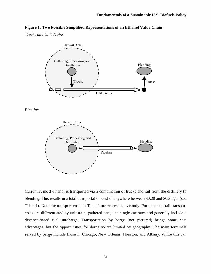
Two options for the basic structure of the ethanol “value chain” are indicated in Figure 1. The
first, labeled “Trucks and Unit Trains,” more closely reflects the current structure of the ethanol
value chain. The second, labeled “Pipeline,” is often discussed as a preferred alternative.
Fundamentals of a Sustainable U.S. Biofuels Policy
31
Figure 1: Two Possible Simplified Representations of an Ethanol Value Chain
Trucks and Unit Trains
Pipeline
Currently, most ethanol is transported via a combination of trucks and rail from the distillery to
blending. This results in a total transportation cost of anywhere between $0.20 and $0.30/gal (see
Table 1). Note the transport costs in Table 1 are representative only. For example, rail transport
costs are differentiated by unit train, gathered cars, and single car rates and generally include a
distance-based fuel surcharge. Transportation by barge (not pictured) brings some cost
advantages, but the opportunities for doing so are limited by geography. The main terminals
served by barge include those in Chicago, New Orleans, Houston, and Albany. While this can
Pipeline
Blending
Harvest Area
Gathering, Processing and
Distillation
Gathering, Processing and
Distillation
Trucks
Unit Trains
Trucks
Blending
Harvest Area
Fundamentals of a Sustainable U.S. Biofuels Policy
32
bring lower transport costs from the Midwest to markets in the Gulf Coast and East Coast, it does
nothing for costs to markets that do not have direct water access, such as those in the West.
Table 1. Representative Distribution Costs by Mode
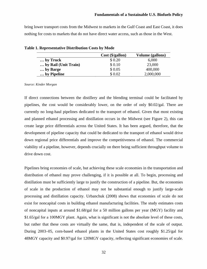
Cost ($/gallon) Volume (gallons)
… by Truck $ 0.20 6,000 … by Rail (Unit Train) $ 0.10 23,000 … by Barge $ 0.05 400,000 … by Pipeline $ 0.02 2,000,000
Source: Kinder Morgan
If direct connections between the distillery and the blending terminal could be facilitated by
pipelines, the cost would be considerably lower, on the order of only $0.02/gal. There are
currently no long-haul pipelines dedicated to the transport of ethanol. Given that most existing
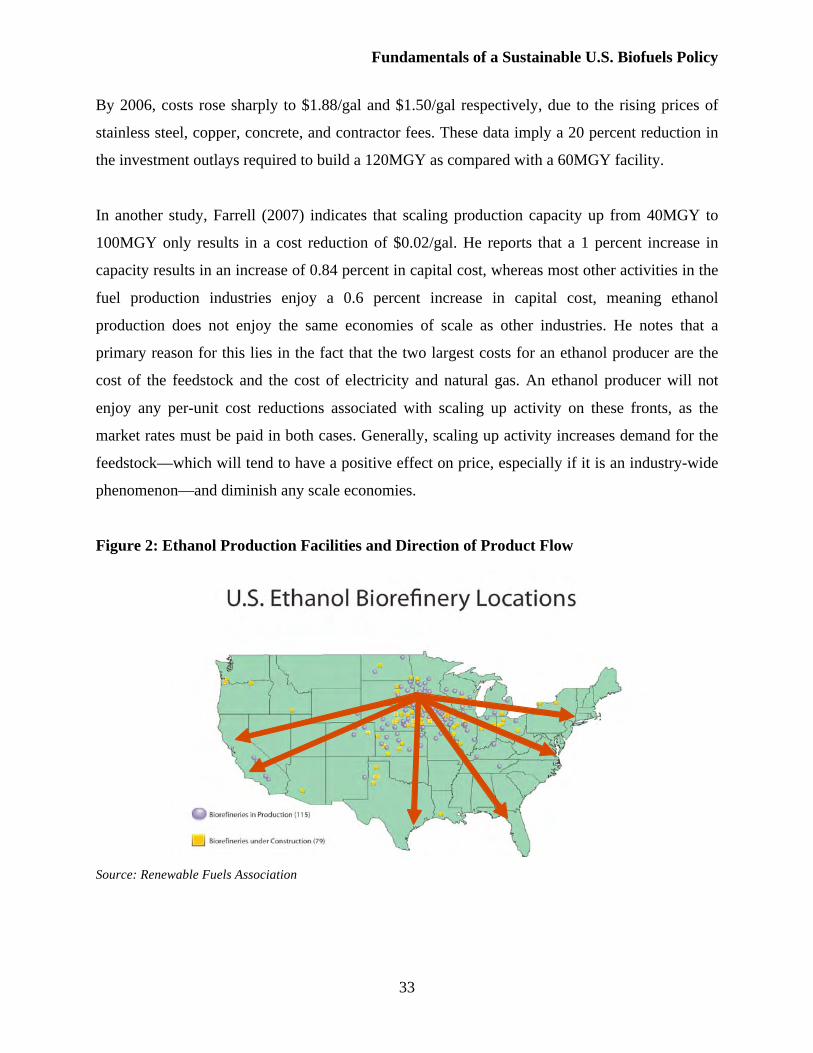
and planned ethanol processing and distillation occurs in the Midwest (see Figure 2), this can
create large price differentials across the United States. It has been argued, therefore, that the
development of pipeline capacity that could be dedicated to the transport of ethanol would drive
down regional price differentials and improve the competitiveness of ethanol. The commercial
viability of a pipeline, however, depends crucially on there being sufficient throughput volume to
drive down cost.
Pipelines bring economies of scale, but achieving these scale economies in the transportation and
distribution of ethanol may prove challenging, if it is possible at all. To begin, processing and
distillation must be sufficiently large to justify the construction of a pipeline. But, the economies
of scale in the production of ethanol may not be substantial enough to justify large-scale
processing and distillation capacity. Urbanchuk (2008) shows that economies of scale do not
exist for noncapital costs in building ethanol manufacturing facilities. The study estimates costs
of noncapital inputs at around $1.68/gal for a 50 million gallons per year (MGY) facility and
$1.65/gal for a 100MGY plant. Again, what is significant is not the absolute level of these costs,
but rather that these costs are virtually the same, that is, independent of the scale of output.
During 2003–05, corn-based ethanol plants in the United States cost roughly $1.25/gal for
48MGY capacity and $0.97/gal for 120MGY capacity, reflecting significant economies of scale.
Fundamentals of a Sustainable U.S. Biofuels Policy
33
By 2006, costs rose sharply to $1.88/gal and $1.50/gal respectively, due to the rising prices of
stainless steel, copper, concrete, and contractor fees. These data imply a 20 percent reduction in
the investment outlays required to build a 120MGY as compared with a 60MGY facility.
In another study, Farrell (2007) indicates that scaling production capacity up from 40MGY to
100MGY only results in a cost reduction of $0.02/gal. He reports that a 1 percent increase in
capacity results in an increase of 0.84 percent in capital cost, whereas most other activities in the
fuel production industries enjoy a 0.6 percent increase in capital cost, meaning ethanol
production does not enjoy the same economies of scale as other industries. He notes that a
primary reason for this lies in the fact that the two largest costs for an ethanol producer are the
cost of the feedstock and the cost of electricity and natural gas. An ethanol producer will not
enjoy any per-unit cost reductions associated with scaling up activity on these fronts, as the
market rates must be paid in both cases. Generally, scaling up activity increases demand for the
feedstock—which will tend to have a positive effect on price, especially if it is an industry-wide
phenomenon—and diminish any scale economies.
Figure 2: Ethanol Production Facilities and Direction of Product Flow
Source: Renewable Fuels Association
Fundamentals of a Sustainable U.S. Biofuels Policy
34
If the scale economies associated with expanding production capacity are indeed minimal, the
chances that investors will choose to build larger facilities are reduced, given the difficulties of
amassing large amounts of biomass in one place. The prevalence of smaller-sized plants reduces
the likelihood that a sufficient production volume will be amassed in a central location to justify
pipeline development. In fact, recent projections by the Washington, D.C.-based Renewable
Fuels Association indicate that the number of ethanol refineries will rise substantially by 2011,
but the average size of production facilities will only increase slightly, rising to about 4,400 b/d
(or about 67MGY). Given the relatively small scale of new developments, a gathering system
would be needed to aggregate production volumes to a central location if pipeline development is
to become economically viable.
A simple model will help to illustrate some important key points regarding the difficulties the
ethanol industry could face when considering expansion. For the sake of exposition, we ignore
the market value of the dried distillers grain used as livestock feed and other by-products. While
the values associated with these products are important, their inclusion is not important for what
follows, and expansion of the model to account for their values is straightforward.
Consider a firm that seeks to maximize the profits from the production and sale of ethanol, ,
from corn, . Ethanol output is a function of capacity, , and capacity utilization, , such that
. Since , in the short run when capacity is fixed, the firm can alter in response
to changes in market variables. In the long run, by contrast, the firm will tend to adjust capacity.
Desired ethanol output determines corn input according to the rule , where
reflects the current state of technology and process efficiency in converting corn to ethanol as
well as the process itself. According to a 2006 USDA study,
“Corn yield per harvested acre is directly related to land quality, management,
weather, farm input use, and advanced technologies used in corn production.
Some of these technologies include genetically modified seed, slow release
fertilizer, global positioning systems (GPS), and yield mapping.”
Fundamentals of a Sustainable U.S. Biofuels Policy
35
To the extent that best-quality acreage is planted and harvested first, the ethanol yield per bushel
of corn harvested could fall as production is expanded. Therefore, we let and
reflect the fact that increasing output will require more corn input and that there may be
diminishing returns to corn inputs. However, innovation in the production process can offset
these negative effects, which is also indicated in the above quote. So, we let account for
technological advances in the ethanol industry.
The ethanol producer receives a netback price, , for its output. The netback price is the price
received from the blender, , less transportation costs from the producer to the blender, or
. The firm takes the price paid by the blender as given, but has some influence over
the transportation cost. In particular, as discussed above, ethanol can be transported to the
blender in multiple ways. For the sake of exposition we consider only two such methods here,
but the problem can be generalized to incorporate others. Consider two methods: (1) low fixed
cost, high variable cost and (2) high fixed cost, low variable cost. If the producer chooses to ship
ethanol using method 1, the total cost is . If the producer chooses to ship by method 2, the total
cost is . The fixed cost of method 2, , is higher than the fixed cost of the method 1, .
The total variable cost of transport rises with throughput in both cases, but the marginal cost of
option 1, , is lower than the marginal cost of the option 2, . Thus, there is a quantity, , at
which the cost of the two options is equal, but above and below that quantity they are not. Thus,
transport costs from the distillery to the blender are given as
where , , , and .
Thus, there is a tradeoff between fixed and variable costs when choosing the mode of
transportation. Specifically, it will only make sense to bear the higher fixed costs of transport via
pipeline if is sufficiently large (see Figure 3). Notably, the average cost of option 2 is lower
than the average cost of option 1 for all .
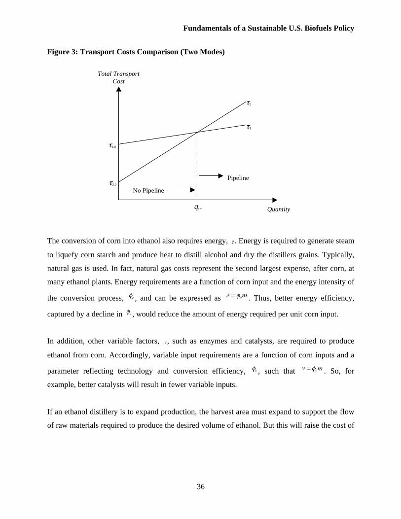
Fundamentals of a Sustainable U.S. Biofuels Policy
36
Figure 3: Transport Costs Comparison (Two Modes)
The conversion of corn into ethanol also requires energy, . Energy is required to generate steam
to liquefy corn starch and produce heat to distill alcohol and dry the distillers grains. Typically,
natural gas is used. In fact, natural gas costs represent the second largest expense, after corn, at
many ethanol plants. Energy requirements are a function of corn input and the energy intensity of
the conversion process, , and can be expressed as . Thus, better energy efficiency,
captured by a decline in , would reduce the amount of energy required per unit corn input.
In addition, other variable factors, , such as enzymes and catalysts, are required to produce
ethanol from corn. Accordingly, variable input requirements are a function of corn inputs and a
parameter reflecting technology and conversion efficiency, , such that . So, for
example, better catalysts will result in fewer variable inputs.
If an ethanol distillery is to expand production, the harvest area must expand to support the flow
of raw materials required to produce the desired volume of ethanol. But this will raise the cost of
1,0
2,0
qsw
1
2
Total Transport
Cost
Quantity
Pipeline
No Pipeline
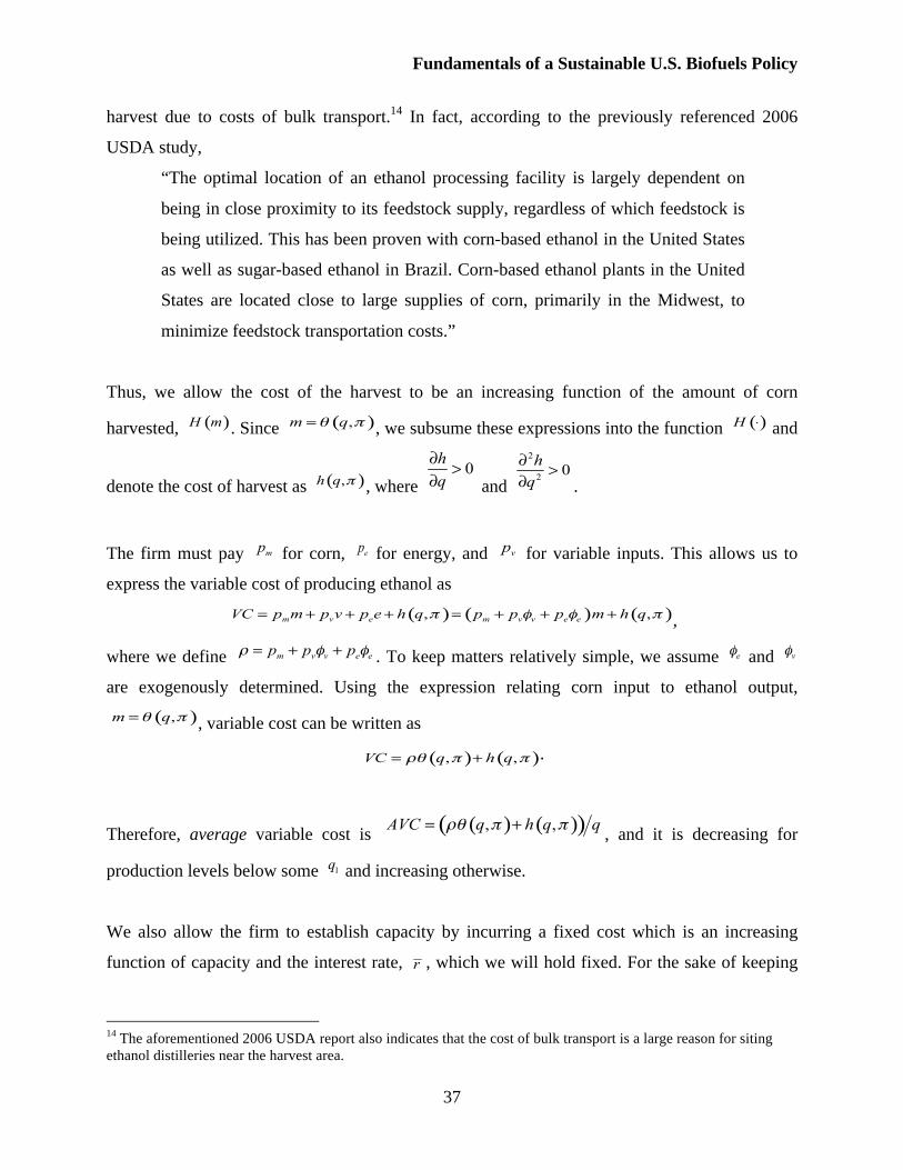
Fundamentals of a Sustainable U.S. Biofuels Policy
37
harvest due to costs of bulk transport.14 In fact, according to the previously referenced 2006
USDA study,
“The optimal location of an ethanol processing facility is largely dependent on
being in close proximity to its feedstock supply, regardless of which feedstock is
being utilized. This has been proven with corn-based ethanol in the United States
as well as sugar-based ethanol in Brazil. Corn-based ethanol plants in the United
States are located close to large supplies of corn, primarily in the Midwest, to
minimize feedstock transportation costs.”
Thus, we allow the cost of the harvest to be an increasing function of the amount of corn
harvested, . Since , we subsume these expressions into the function and
denote the cost of harvest as , where and .
The firm must pay for corn, for energy, and for variable inputs. This allows us to
express the variable cost of producing ethanol as
,
where we define . To keep matters relatively simple, we assume and
are exogenously determined. Using the expression relating corn input to ethanol output,
, variable cost can be written as
.
Therefore, average variable cost is , and it is decreasing for
production levels below some and increasing otherwise.
We also allow the firm to establish capacity by incurring a fixed cost which is an increasing
function of capacity and the interest rate, , which we will hold fixed. For the sake of keeping
14 The aforementioned 2006 USDA report also indicates that the cost of bulk transport is a large reason for siting
ethanol distilleries near the harvest area.
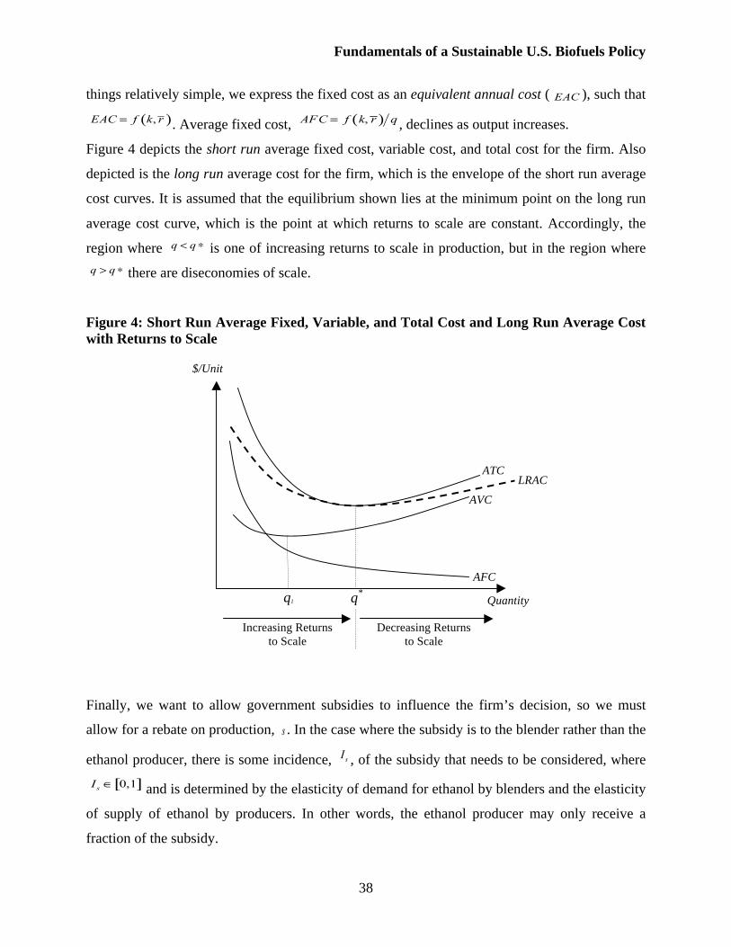
Fundamentals of a Sustainable U.S. Biofuels Policy
38
things relatively simple, we express the fixed cost as an equivalent annual cost ( ), such that
. Average fixed cost, , declines as output increases.
Figure 4 depicts the short run average fixed cost, variable cost, and total cost for the firm. Also
depicted is the long run average cost for the firm, which is the envelope of the short run average
cost curves. It is assumed that the equilibrium shown lies at the minimum point on the long run
average cost curve, which is the point at which returns to scale are constant. Accordingly, the
region where is one of increasing returns to scale in production, but in the region where
there are diseconomies of scale.
Figure 4: Short Run Average Fixed, Variable, and Total Cost and Long Run Average Cost
with Returns to Scale
Finally, we want to allow government subsidies to influence the firm’s decision, so we must
allow for a rebate on production, . In the case where the subsidy is to the blender rather than the
ethanol producer, there is some incidence, , of the subsidy that needs to be considered, where
and is determined by the elasticity of demand for ethanol by blenders and the elasticity
of supply of ethanol by producers. In other words, the ethanol producer may only receive a
fraction of the subsidy.
$/Unit
Quantity
AFC
AVC
Increasing Returns
to Scale
q*
q1
Decreasing Returns
to Scale
LRAC ATC
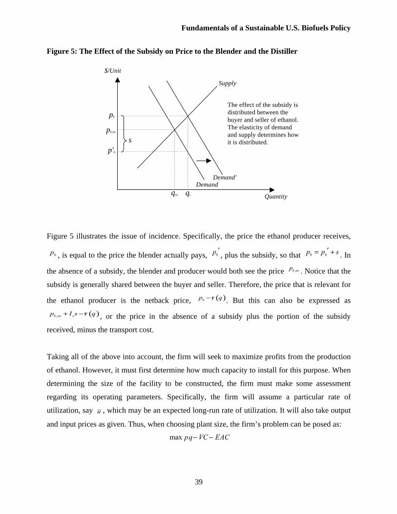
Fundamentals of a Sustainable U.S. Biofuels Policy
39
Figure 5: The Effect of the Subsidy on Price to the Blender and the Distiller
Figure 5 illustrates the issue of incidence. Specifically, the price the ethanol producer receives,
, is equal to the price the blender actually pays, , plus the subsidy, so that . In
the absence of a subsidy, the blender and producer would both see the price . Notice that the
subsidy is generally shared between the buyer and seller. Therefore, the price that is relevant for
the ethanol producer is the netback price, . But this can also be expressed as
, or the price in the absence of a subsidy plus the portion of the subsidy
received, minus the transport cost.
Taking all of the above into account, the firm will seek to maximize profits from the production
of ethanol. However, it must first determine how much capacity to install for this purpose. When
determining the size of the facility to be constructed, the firm must make some assessment
regarding its operating parameters. Specifically, the firm will assume a particular rate of
utilization, say , which may be an expected long-run rate of utilization. It will also take output
and input prices as given. Thus, when choosing plant size, the firm’s problem can be posed as:
$/Unit
Quantity
Demand
Supply
The effect of the subsidy is
distributed between the
buyer and seller of ethanol.
The elasticity of demand
and supply determines how
it is distributed.
qns
Demand'
qs
p'b
pb
pb,ns
s
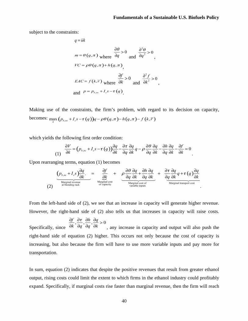
Fundamentals of a Sustainable U.S. Biofuels Policy
40
subject to the constraints:
where and ,
,
where and ,
and .
Making use of the constraints, the firm’s problem, with regard to its decision on capacity,
becomes:
which yields the following first order condition:
(1) .
Upon rearranging terms, equation (1) becomes
(2) .
From the left-hand side of (2), we see that an increase in capacity will generate higher revenue.
However, the right-hand side of (2) also tells us that increases in capacity will raise costs.
Specifically, since , any increase in capacity and output will also push the
right-hand side of equation (2) higher. This occurs not only because the cost of capacity is
increasing, but also because the firm will have to use more variable inputs and pay more for
transportation.
In sum, equation (2) indicates that despite the positive revenues that result from greater ethanol
output, rising costs could limit the extent to which firms in the ethanol industry could profitably
expand. Specifically, if marginal costs rise faster than marginal revenue, then the firm will reach
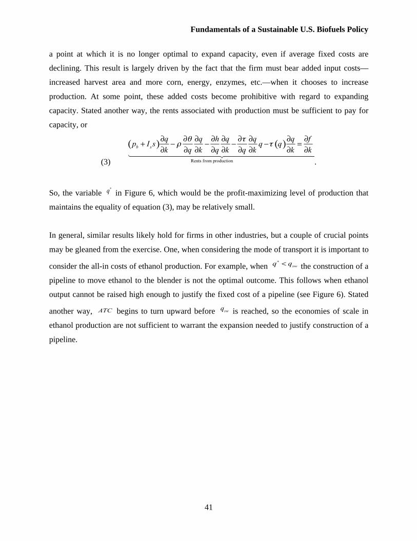
Fundamentals of a Sustainable U.S. Biofuels Policy
41
a point at which it is no longer optimal to expand capacity, even if average fixed costs are
declining. This result is largely driven by the fact that the firm must bear added input costs—
increased harvest area and more corn, energy, enzymes, etc.—when it chooses to increase
production. At some point, these added costs become prohibitive with regard to expanding
capacity. Stated another way, the rents associated with production must be sufficient to pay for
capacity, or
(3) .
So, the variable in Figure 6, which would be the profit-maximizing level of production that
maintains the equality of equation (3), may be relatively small.
In general, similar results likely hold for firms in other industries, but a couple of crucial points
may be gleaned from the exercise. One, when considering the mode of transport it is important to
consider the all-in costs of ethanol production. For example, when the construction of a
pipeline to move ethanol to the blender is not the optimal outcome. This follows when ethanol
output cannot be raised high enough to justify the fixed cost of a pipeline (see Figure 6). Stated
another way, begins to turn upward before is reached, so the economies of scale in
ethanol production are not sufficient to warrant the expansion needed to justify construction of a
pipeline.
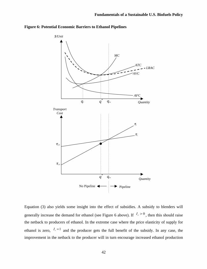
Fundamentals of a Sustainable U.S. Biofuels Policy
42
Figure 6: Potential Economic Barriers to Ethanol Pipelines
Equation (3) also yields some insight into the effect of subsidies. A subsidy to blenders will
generally increase the demand for ethanol (see Figure 6 above). If , then this should raise
the netback to producers of ethanol. In the extreme case where the price elasticity of supply for
ethanol is zero, and the producer gets the full benefit of the subsidy. In any case, the
improvement in the netback to the producer will in turn encourage increased ethanol production
qsw
$/Unit
Quantity
AFC
AVC
ATC
MC
2,0
1,0
qsw
2
1
Pipeline No Pipeline
Transport
Cost
Quantity
q*
q*
q1
LRAC
Fundamentals of a Sustainable U.S. Biofuels Policy
43
and greater capacity. If the subsidy is large enough, it is possible that production could expand
such that , in which case a pipeline could be profitably constructed.
However, the story may not be so simple. Specifically, a subsidy may not have this intended
first-order effect. In particular, according to the Stolper-Samuelson Theorem, increased output of
ethanol should raise the price of the input that is used most intensely.15 Thus, the subsidy, by
encouraging production, could have the unintended effect of raising corn prices and even land
prices, which would act as a counterweight to the first-order expansionary effect of the subsidy.
More specifically, if increased output substantially raises the price of corn and other inputs, then
the marginal cost of variable inputs, , will rise, thereby diminishing the intended
impact of the subsidy. In fact, if the subsidy also raises the price of land, it would further raise
costs and possibly even present barriers to entry into the business of ethanol production.
The fact that input costs could increase as a result of a subsidy has substantial ramifications for
policies aimed at encouraging the expansion of the ethanol industry. If subsidies ultimately raise
the cost of inputs used most intensively in the targeted industry, then the subsidies may not have
the desired effect, particularly if the second-order effect on input prices is substantial. Thus, the
ethanol industry may be incapable of expanding significantly in its current state.
The ethanol industry might best be promoted through increased efficiency in the production
process. Policies that target efficiency gains, perhaps through grants for R&D, would reduce ,
, and in the model presented above, and promote expansion by lowering the marginal cost
of variable inputs. Importantly, the efficiency gains would have to be substantial enough to offset
any increases in the input prices that might also occur with expansion. This latter point is
consistent with comments by Madson and Monceaux (2003), who state:
15 The Stolper-Samuelson Theorem states that an increase in the price of a good will cause an increase in the price of
the factor used intensively in that industry and a decrease in the price of other factors.
Fundamentals of a Sustainable U.S. Biofuels Policy
44
“Most MFGE (motor fuel grade ethanol) producers have little control over
feedstock pricing beyond hedging strategies such as trading in futures. The
producers’ primary edge is therefore to maximize yield.”
This sentiment is reinforced by the model presented above, and, in fact, yields have been
increasing since the 1980s. The question remains, however, as to how high yields must be to
support substantial industry expansion, especially without subsidies.
This is also echoed by the EIA’s report in the 2007 Annual Energy Outlook. Specifically:
“There have been large annual increases in yields of both corn and soybeans over
the past 30 years. Corn yields increased from 86.4 bushels per acre in 1975 to
151.2 bushels per acre in 2006 … If corn yields continue to increase at the same
rate (approximately 1.8 bushels per acre per year), production could increase by
more than 3.1 billion bushels (29 percent) by 2030 without requiring any
additional acreage … Improvements in biofuel collection and refining and
bioengineering of corn and soybeans also could contribute to improved biofuel
yields.” (DOE, EIA 2007).
Therefore, a common theme in studying the economic viability of ethanol expansion is one of
“more R&D.” If advances in productivity continue, the necessity of subsidies may be
diminished. Moreover, improvements in productivity could open up significant expansion
opportunities that could dramatically change the manner in which ethanol is transported.
V. Ethanol Transportation Costs, Part Two: A Role for Imports
Improvements in technologies that reduce transport and manufacturing costs are vital to an
ethanol industry that is to survive in a competitive landscape against other fuels and other
sources of ethanol. Some of the biggest logistical difficulties facing greater ethanol penetration in
the U.S. fuel supply are directly related to cost. In fact, current government support is required
for ethanol produced in the Midwest to be an attractive option to blenders in most other parts of
the country. Moreover, even with a blender credit of $0.45 and a $0.54 tariff on foreign-sourced
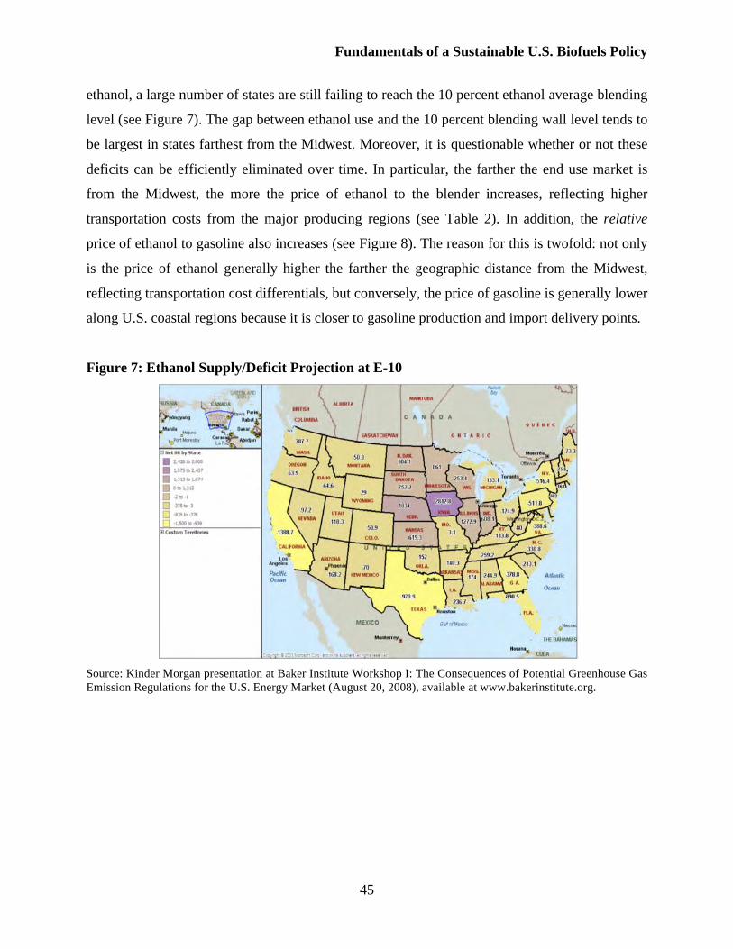
Fundamentals of a Sustainable U.S. Biofuels Policy
45
ethanol, a large number of states are still failing to reach the 10 percent ethanol average blending
level (see Figure 7). The gap between ethanol use and the 10 percent blending wall level tends to
be largest in states farthest from the Midwest. Moreover, it is questionable whether or not these
deficits can be efficiently eliminated over time. In particular, the farther the end use market is
from the Midwest, the more the price of ethanol to the blender increases, reflecting higher
transportation costs from the major producing regions (see Table 2). In addition, the relative
price of ethanol to gasoline also increases (see Figure 8). The reason for this is twofold: not only
is the price of ethanol generally higher the farther the geographic distance from the Midwest,
reflecting transportation cost differentials, but conversely, the price of gasoline is generally lower
along U.S. coastal regions because it is closer to gasoline production and import delivery points.
Figure 7: Ethanol Supply/Deficit Projection at E-10
Source: Kinder Morgan presentation at Baker Institute Workshop I: The Consequences of Potential Greenhouse Gas
Emission Regulations for the U.S. Energy Market (August 20, 2008), available at www.bakerinstitute.org.
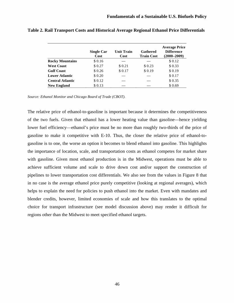
Fundamentals of a Sustainable U.S. Biofuels Policy
46
Table 2. Rail Transport Costs and Historical Average Regional Ethanol Price Differentials
Single Car
Cost
Unit Train
Cost
Gathered
Train Cost
Average Price
Difference
(2000–2009)
Rocky Mountains $ 0.16 --- --- $ 0.12
West Coast $ 0.27 $ 0.21 $ 0.23 $ 0.33
Gulf Coast $ 0.26 $ 0.17 $ 0.19 $ 0.19
Lower Atlantic $ 0.20 --- --- $ 0.17
Central Atlantic $ 0.12 --- --- $ 0.35
New England $ 0.13 --- --- $ 0.69
Source: Ethanol Monitor and Chicago Board of Trade (CBOT).
The relative price of ethanol-to-gasoline is important because it determines the competitiveness
of the two fuels. Given that ethanol has a lower heating value than gasoline—hence yielding
lower fuel efficiency—ethanol’s price must be no more than roughly two-thirds of the price of
gasoline to make it competitive with E-10. Thus, the closer the relative price of ethanol-to-
gasoline is to one, the worse an option it becomes to blend ethanol into gasoline. This highlights
the importance of location, scale, and transportation costs as ethanol competes for market share
with gasoline. Given most ethanol production is in the Midwest, operations must be able to
achieve sufficient volume and scale to drive down cost and/or support the construction of
pipelines to lower transportation cost differentials. We also see from the values in Figure 8 that
in no case is the average ethanol price purely competitive (looking at regional averages), which
helps to explain the need for policies to push ethanol into the market. Even with mandates and
blender credits, however, limited economies of scale and how this translates to the optimal
choice for transport infrastructure (see model discussion above) may render it difficult for
regions other than the Midwest to meet specified ethanol targets.
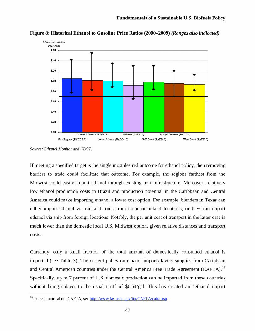
Fundamentals of a Sustainable U.S. Biofuels Policy
47
Figure 8: Historical Ethanol to Gasoline Price Ratios (2000–2009) (Ranges also indicated)
Source: Ethanol Monitor and CBOT.
If meeting a specified target is the single most desired outcome for ethanol policy, then removing
barriers to trade could facilitate that outcome. For example, the regions farthest from the
Midwest could easily import ethanol through existing port infrastructure. Moreover, relatively
low ethanol production costs in Brazil and production potential in the Caribbean and Central
America could make importing ethanol a lower cost option. For example, blenders in Texas can
either import ethanol via rail and truck from domestic inland locations, or they can import
ethanol via ship from foreign locations. Notably, the per unit cost of transport in the latter case is
much lower than the domestic local U.S. Midwest option, given relative distances and transport
costs.
Currently, only a small fraction of the total amount of domestically consumed ethanol is
imported (see Table 3). The current policy on ethanol imports favors supplies from Caribbean
and Central American countries under the Central America Free Trade Agreement (CAFTA).16
Specifically, up to 7 percent of U.S. domestic production can be imported from these countries
without being subject to the usual tariff of $0.54/gal. This has created an “ethanol import
16 To read more about CAFTA, see http://www.fas.usda.gov/itp/CAFTA/cafta.asp.
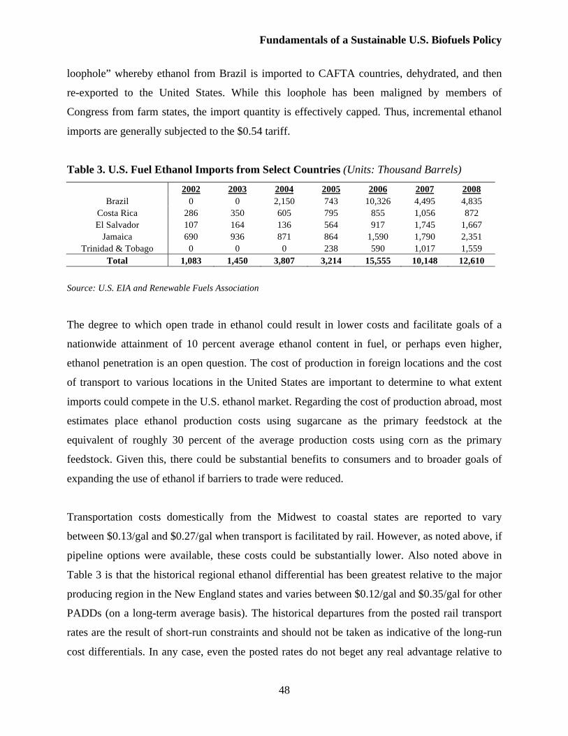
Fundamentals of a Sustainable U.S. Biofuels Policy
48
loophole” whereby ethanol from Brazil is imported to CAFTA countries, dehydrated, and then
re-exported to the United States. While this loophole has been maligned by members of
Congress from farm states, the import quantity is effectively capped. Thus, incremental ethanol
imports are generally subjected to the $0.54 tariff.
Table 3. U.S. Fuel Ethanol Imports from Select Countries (Units: Thousand Barrels)
2002 2003 2004 2005 2006 2007 2008
Brazil 0 0 2,150 743 10,326 4,495 4,835
Costa Rica 286 350 605 795 855 1,056 872
El Salvador 107 164 136 564 917 1,745 1,667
Jamaica 690 936 871 864 1,590 1,790 2,351
Trinidad & Tobago 0 0 0 238 590 1,017 1,559
Total 1,083 1,450 3,807 3,214 15,555 10,148 12,610
Source: U.S. EIA and Renewable Fuels Association
The degree to which open trade in ethanol could result in lower costs and facilitate goals of a
nationwide attainment of 10 percent average ethanol content in fuel, or perhaps even higher,
ethanol penetration is an open question. The cost of production in foreign locations and the cost
of transport to various locations in the United States are important to determine to what extent
imports could compete in the U.S. ethanol market. Regarding the cost of production abroad, most
estimates place ethanol production costs using sugarcane as the primary feedstock at the
equivalent of roughly 30 percent of the average production costs using corn as the primary
feedstock. Given this, there could be substantial benefits to consumers and to broader goals of
expanding the use of ethanol if barriers to trade were reduced.
Transportation costs domestically from the Midwest to coastal states are reported to vary
between $0.13/gal and $0.27/gal when transport is facilitated by rail. However, as noted above, if
pipeline options were available, these costs could be substantially lower. Also noted above in
Table 3 is that the historical regional ethanol differential has been greatest relative to the major
producing region in the New England states and varies between $0.12/gal and $0.35/gal for other
PADDs (on a long-term average basis). The historical departures from the posted rail transport
rates are the result of short-run constraints and should not be taken as indicative of the long-run
cost differentials. In any case, even the posted rates do not beget any real advantage relative to
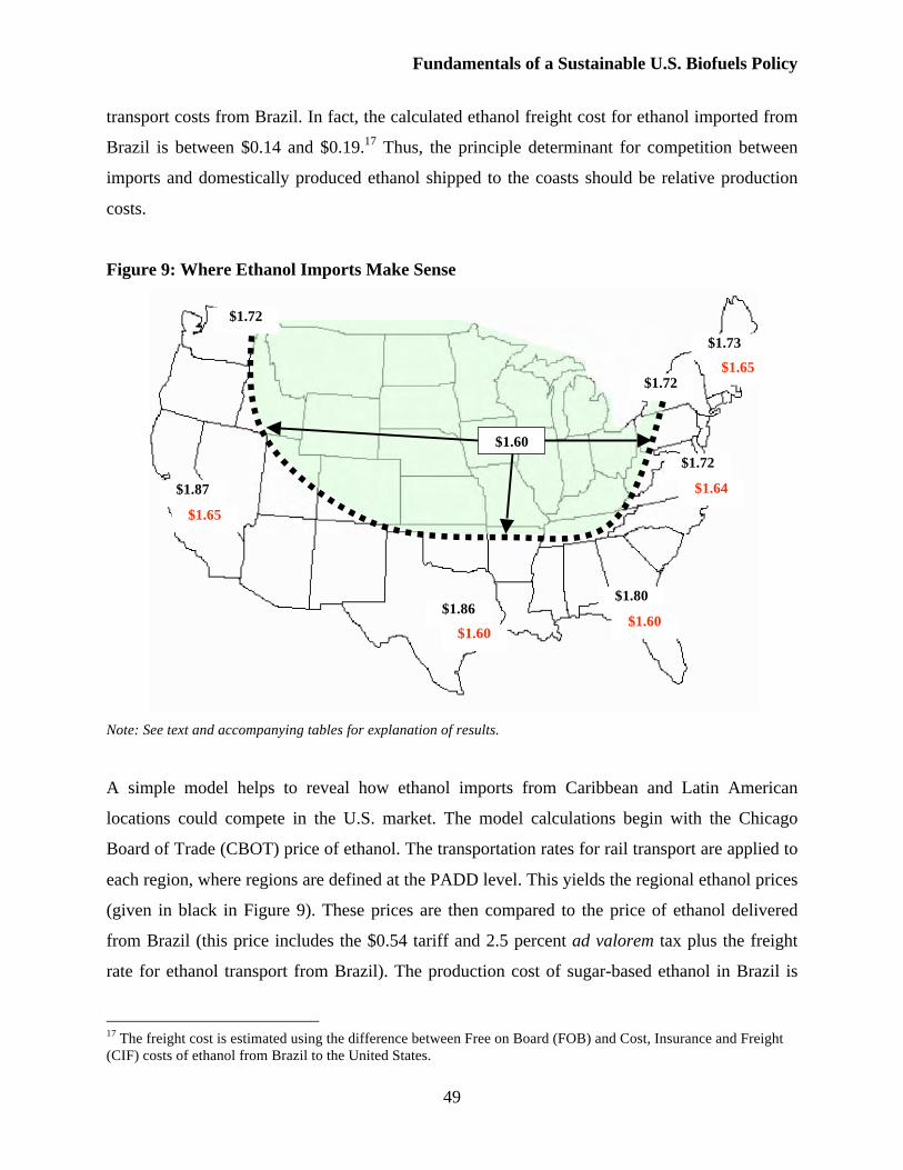
Fundamentals of a Sustainable U.S. Biofuels Policy
49
transport costs from Brazil. In fact, the calculated ethanol freight cost for ethanol imported from
Brazil is between $0.14 and $0.19.17 Thus, the principle determinant for competition between
imports and domestically produced ethanol shipped to the coasts should be relative production
costs.
Figure 9: Where Ethanol Imports Make Sense
Note: See text and accompanying tables for explanation of results.
A simple model helps to reveal how ethanol imports from Caribbean and Latin American
locations could compete in the U.S. market. The model calculations begin with the Chicago
Board of Trade (CBOT) price of ethanol. The transportation rates for rail transport are applied to
each region, where regions are defined at the PADD level. This yields the regional ethanol prices
(given in black in Figure 9). These prices are then compared to the price of ethanol delivered
from Brazil (this price includes the $0.54 tariff and 2.5 percent ad valorem tax plus the freight
rate for ethanol transport from Brazil). The production cost of sugar-based ethanol in Brazil is
17 The freight cost is estimated using the difference between Free on Board (FOB) and Cost, Insurance and Freight
(CIF) costs of ethanol from Brazil to the United States.
$1.72
$1.72
$1.86 $1.80
$1.87
$1.60
$1.73
$1.72
$1.60 $1.60
$1.65
$1.64
$1.65
Fundamentals of a Sustainable U.S. Biofuels Policy
50
taken as $0.88/gal. The resulting prices for Brazilian ethanol delivered to the United States range
from $1.60/gal to $1.65/gal, inclusive of the tariff costs.
Comparing a case with an import tariff and a U.S. blender’s credit and a case without any tariff
or subsidy, we see that the results are dramatically different, supporting the notion that the
current tariff is effective in its protection of the domestic ethanol industry. Absent any
government support, it is likely that domestic production would fall dramatically because, in that
case, Brazilian imports could land economically in the U.S. coastal markets for just over
$1.00/gal, representing a $0.60/gal savings over prices currently perpetuated by the tariff and ad
valorem tax. Arguably, this would make importing and shipping gasoline blended fuels inland
from the coasts using existing fuel delivery infrastructure (i.e., product pipelines) much more
attractive than producing ethanol domestically in the Midwest and shipping it to coastal areas.
However, with the current tariff and subsidy scheme in place, the arbitrage point lies such that
expansion of the domestic ethanol industry makes sense, at least until the Midwest and Rocky
Mountain States demands are met (see Figure 9). Beyond that, innovation will have to drive
down production and transportation costs—which, as we saw above, are not necessarily mutually
exclusive—if domestic ethanol is to compete longer term for the large coastal U.S. markets.
Feedstock and energy costs can be highly variable, so we compared several cases in which these
costs were allowed to change. But in none of the cases did the answer substantially change.
While the arbitrage point can move slightly, the largest fuel-consuming markets in the United
States—and hence largest potential ethanol consuming regions—are in California, Texas,
Florida, and the Northeast. The arbitrage point between ethanol produced in the Midwest and
ethanol imported from Brazil (represented by the dotted lines in Figure 9) does not extend
beyond these markets in any of the variants considered. In fact, for the arbitrage point to
encompass the entire lower 48, thus disadvantaging imports, corn-based ethanol prices must fall
by about $0.20/gal. To keep the crush spread at current levels (roughly $0.37 for corn prices at
$3.50/bushel and ethanol at $1.60 on the CBOT), corn prices would have to fall just below
$3.00/bushel. Of course, if the import tariff were lifted, these costs would have to fall by an even
greater amount.
Fundamentals of a Sustainable U.S. Biofuels Policy
51
In sum, the coastal U.S. regions would benefit from open trade. The obvious drawback is that
domestic ethanol production will be slightly lower, a result that will undoubtedly not sit well
with policymakers from farm states. Nevertheless, every region of the country would be able to
hit its E-10 target at a lower cost, were import tariffs to be removed.
The results indicate that imports should grow beyond the current small fraction of the total U.S.
market. Moreover, imports should grow beyond those quantities that can be imported from
Caribbean and Central American countries under the tariff-free quota (which amounts to 7
percent of the U.S. market) if E-10 requirements are to be met in the least-cost manner.
However, production capacity in countries that could expand exports to the United States would
have to grow to saturate the U.S. market. This is a difficult proposition. For foreign producers to
make large-scale investments in ethanol production capability for export to the United States
requires some certainty that the market will be viable. If the U.S. government intends to protect
its domestic ethanol industry, then it may raise tariffs, impose quotas, increase blenders’ credits,
or any other myriad of possibilities. If foreign producers see this as a possibility, they will be
reluctant to incur a sunk cost, which they may never recover, should domestic politics continue
to point toward domestic industry protectionism.
VI. Ethanol Production Potential of Select Latin American Countries
In this section, we estimate the potential of several countries in Latin America to produce more
sugarcane-based ethanol for export, possibly to the United States. The most reliable estimate is
for Cuba, a country that once had a thriving sugar industry that has collapsed since the fall of the
Soviet Union. The estimate in that country is based on the assumption that Cuba can revive the
industry and plant areas comparable to those during the era of Soviet trade, but with yields closer
to those currently being achieved in other countries in the region.
For other countries our estimate is, of necessity, a bit more uncertain because we must make
assumptions about what acreage of available land can be devoted to sugarcane without detailed
knowledge of whether all of the conditions for cultivation—such as temperature, water, and soil
Fundamentals of a Sustainable U.S. Biofuels Policy
52
conditions—are met.18 In addition, there is the issue of whether sugarcane cultivation can be
extended without impinging on food production.19
Ethanol Potential in Cuba
Cuba was a major sugar producer and exporter throughout most of the twentieth century. In fact,
it was a major source of U.S. sugar imports before the Cuban Revolution. Later, Cuba became
the primary supplier for the Soviet Union in the 1970s and 1980s. However, with the collapse of
the Soviet Union, Cuba’s sugar production fell to 1.2 million metric tons (1.3 million tons) in
2007, down from 8.1 million metric tons (8.9 million tons) in 1988. Harvested acreage of
sugarcane followed suit, falling from 1.45 million hectares, approximately 3.6 million acres, in
1991 and 1992 to only 400,000 hectares (about 1 million acres) in 2007. Finally, according to
statistics from the Food and Agriculture Organization of the United Nations (FAOSTAT),
sugarcane yields fell from 50 to 60 metric tons per hectare (t/ha), the equivalent of 22 to 27 tons
per acre (tn/ac), in the 1970s and 1980s to only 28 t/ha (12.5 tn/ac) in 2007. As a result, sugar
mills have been closed and large numbers of workers have been retrained and moved off the
land.
Despite the past scale of the sugar industry in Cuba, if Cuba were to today choose to develop its
ethanol industry, there are some questions as to how much land could be devoted to sugarcane.
Cuba currently has a policy of promoting greater land use for food production. According to
FAOSTAT, during the period 1970–1990, the average area harvested was 1.3 million hectares
(3.2 million acres), and it may be difficult to sustain levels much higher than that. Some of the
land that has been idle since the decline of the sugar industry has been converted to food crops in
an effort to reduce food imports. Other land is earmarked for forest development, and there have
18 Regarding conditions for cultivation, we are confident that our assumptions are reasonable since we are confining
ourselves to countries that lie well within areas where temperatures and, for the most part, rainfall are favorable for
sugarcane production. When it comes to soil conditions, sugarcane is not a demanding crop. Nonetheless, we have
followed a very conservative methodology in making our projections. We give high and low estimates but our high
estimates may very well be far short of these countries’ capabilities. 19 The trade-off with food production has been a contentious one of late. It should be pointed out, however, that if one or a few countries shift land from food crops to sugarcane that does not necessarily imply a reduction in world
food output. Other countries might well increase food output in response to a decrease elsewhere. Indeed, it makes
sense, for example, for the United States with a more temperate climate to produce corn and other food crops for
export rather than to convert them into ethanol and have other countries, more suitably located, to specialize to a
greater extent in the production of sugarcane for ethanol.
Fundamentals of a Sustainable U.S. Biofuels Policy
53
been recent discussions of investing in soybeans. However, given that Cuba has had a traditional
comparative advantage in the production of sugar, the diversion of land to other uses may reflect
the effects of economic sanctions that tend to encourage autarky where possible and promote
export crops that can be sold in markets other than the United States. With the removal of the
U.S.-imposed sanctions on imported ethanol, Cuba could arguably recapture its comparative
advantage in sugar, which would ease the pressure to be self-sufficient in food production. Thus,
acreage that has been diverted to other uses could return to sugarcane cultivation.
In Nicaragua and Brazil, growers have been getting agricultural yields of 75 to 80 t/ha (33 to 36
tn/ac) of sugarcane, and distillers have been achieving yields of 70 to 80 liters per metric ton
(L/t) of sugarcane, roughly 17 to 19 gallons per ton (gal/tn). At 75 t/ha and 75 L/t (5,625 L/ha, or
600 gal/ac), Cuba would need 1.33 million hectares (3.3 million acres) to produce 2 billion
gallons of ethanol. Moreover, agricultural productivity is continually improving as new plant
varieties and new cultivation practices are developed through research and innovation. In some
regions of Brazil, yields of 84 t/ha (37 tn/ac) and 82 L/t (20 gal/tn) of sugarcane (6,888 L/ha, or
750 gal/ac) have been achieved, and even higher yields have been achieved in some areas of São
Paulo. If similar yields were reached in Cuba, ethanol production could reach 2 billion gallons
with only 1.1 million hectares (2.8 million acres) of harvested land.
These production targets are ambitious and cannot be attained in a short period of time. For one,
increasing the land acreage devoted to sugarcane will take time and substantial investment. The
land has been neglected, and much of it has suffered from compaction with the use of very heavy
Soviet built harvesting machinery (Pollitt 2004). So, the land will have to be newly planted with
sugarcane. Beyond that, harvesting machinery has not been maintained, so much of that
equipment will likely have to be replaced.
Downstream of harvest, significant investment is also required. Many sugar mills have been
closed and those that remain have not been properly maintained (Perez-Lopez 2003; Mesa-Lago
2005). Cuba will have to undertake significant investments in distillation, transportation, storage,
and distribution infrastructure if it is to produce substantial levels of ethanol. It is likely that the
scale of investment necessary will run well into the billions of dollars.
Fundamentals of a Sustainable U.S. Biofuels Policy
54
Cuba has opened the door to foreign investment in the ethanol sector and may have a future
partner in Brazil. Specifically, Brazil has expressed interest in sharing its expertise with other
ethanol producers in order to promote the development of an active and liquid ethanol market.
There are also indications that Havana is considering opening access to Cuban land to foreign
companies. With flexible policies and tariff-free access to the U.S. market, Cuba would have no
difficulty finding the foreign investment needed to finance the rapid development of an ethanol
industry. However, current U.S. policy toward Cuba renders the likelihood of trade very low.
Ethanol Potential in Brazil
At the time of the rapid oil price increases in the 1970s, many countries, including the United
States, looked at ethanol as a substitute for oil. However, when oil prices collapsed by the mid-
1980s, interest waned—except in Brazil. The Brazilian government introduced Proálcool, its
national alcohol program, in 1975. Today, Brazil is the world’s largest ethanol exporter.
However, it took Brazil many years and substantial subsidies, which have been phased out, to
reach current production levels.
Brazil’s approach to promoting ethanol use was to mandate that gasoline be mixed with 10
percent ethanol and that this should be increased to 25 percent by 1980 (Colares 2008). In
addition, the government provided loans for the construction of ethanol plants and guaranteed the
price of ethanol. Following the second oil price spike in 1980, the government required
Petrobras, the state-owned oil company, to supply ethanol to filling stations. In order to promote
the substitution of ethanol for gasoline, the Brazilian government also introduced subsidies for
automakers for the production of vehicles that could run on E-100. The market for these cars
collapsed along with oil prices in the 1980s; however, the market for vehicles using ethanol was
restored in the early 2000s with the introduction of flex-fuel vehicles (FFVs) that can operate
using either ethanol or gasoline. FFVs now account for roughly 85 percent of new car sales in
Brazil.
Fundamentals of a Sustainable U.S. Biofuels Policy
55
One estimate puts Brazilian government subsidies from 1979 to the mid-1990s at over $16
billion in 2005 dollars.20 Brazil is now the world’s second-largest producer of ethanol with
output at 6.9 billion gallons (out of world production of 20.4 billion gallons) in 2008, a
significant increase from 2004 when only 3.8 billion gallons were produced. Much of the
increased production has come from increasing the acreage devoted to sugarcane cultivation.
But, productivity of sugarcane has also increased substantially over time, reaching an average of
65 tones/ha. In some regions in São Paulo, yields have reached 100 to 110 t/ha (45 to 49 tn/ac),
representing a 33 percent increase since the mid-1970s. Plans are to increase production in São
Paulo by 50 percent between 2008 and 2010.
Brazil is the largest exporter of ethanol—some 1.3 billion gallons to 48 countries in 2008. In that
year, it sent about 296.2 million gallons to Jamaica, El Salvador, Trinidad and Tobago, and Costa
Rica.21 Much of this is hydrous ethanol, which is then converted to anhydrous ethanol and
exported to the United States under the tariff free provisions of CAFTA.
Other Countries in Latin America and the Caribbean
Table 4 indicates the amount of agricultural land in Western Hemisphere countries that lies in the
tropical zone. The Food and Agricultural Organization of the United Nations (FAO) defines
agricultural area to be the sum of the following:
“(a) arable land - land under temporary crops (double-cropped areas are counted
only once), temporary meadows for mowing or pasture, land under market and
kitchen gardens and land temporarily fallow (less than five years). The abandoned
land resulting from shifting cultivation is not included in this category. (b)
permanent crops - land cultivated with crops that occupy the land for long periods
and need not be replanted after each harvest, such as cocoa, coffee and rubber;
this category includes land under flowering shrubs, fruit trees, nut trees and vines,
but excludes land under trees grown for wood or timber; and (c) permanent
pastures - land used permanently (five years or more) for herbaceous forage
20 Datagro, cited on p. 12 of draft conference report “Biomass to Chemicals and Fuels: Science, Technology, and
Public Policy,” September 25–26, 2006, Baker Institute. 21 Brazilian Sugarcane Industry Association – UNICA.
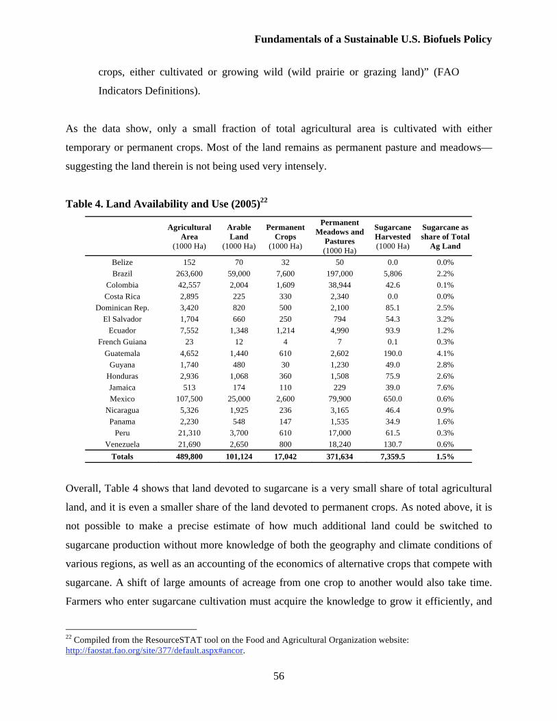
Fundamentals of a Sustainable U.S. Biofuels Policy
56
crops, either cultivated or growing wild (wild prairie or grazing land)” (FAO
Indicators Definitions).
As the data show, only a small fraction of total agricultural area is cultivated with either
temporary or permanent crops. Most of the land remains as permanent pasture and meadows—
suggesting the land therein is not being used very intensely.
Table 4. Land Availability and Use (2005)22
Agricultural
Area
(1000 Ha)
Arable
Land (1000 Ha)
Permanent
Crops (1000 Ha)
Permanent
Meadows and
Pastures (1000 Ha)
Sugarcane
Harvested (1000 Ha)
Sugarcane as
share of Total
Ag Land
Belize 152 70 32 50 0.0 0.0%
Brazil 263,600 59,000 7,600 197,000 5,806 2.2%
Colombia 42,557 2,004 1,609 38,944 42.6 0.1%
Costa Rica 2,895 225 330 2,340 0.0 0.0%
Dominican Rep. 3,420 820 500 2,100 85.1 2.5%
El Salvador 1,704 660 250 794 54.3 3.2%
Ecuador 7,552 1,348 1,214 4,990 93.9 1.2%
French Guiana 23 12 4 7 0.1 0.3%
Guatemala 4,652 1,440 610 2,602 190.0 4.1%
Guyana 1,740 480 30 1,230 49.0 2.8%
Honduras 2,936 1,068 360 1,508 75.9 2.6%
Jamaica 513 174 110 229 39.0 7.6%
Mexico 107,500 25,000 2,600 79,900 650.0 0.6%
Nicaragua 5,326 1,925 236 3,165 46.4 0.9%
Panama 2,230 548 147 1,535 34.9 1.6%
Peru 21,310 3,700 610 17,000 61.5 0.3%
Venezuela 21,690 2,650 800 18,240 130.7 0.6%
Totals 489,800 101,124 17,042 371,634 7,359.5 1.5%
Overall, Table 4 shows that land devoted to sugarcane is a very small share of total agricultural
land, and it is even a smaller share of the land devoted to permanent crops. As noted above, it is
not possible to make a precise estimate of how much additional land could be switched to
sugarcane production without more knowledge of both the geography and climate conditions of
various regions, as well as an accounting of the economics of alternative crops that compete with
sugarcane. A shift of large amounts of acreage from one crop to another would also take time.
Farmers who enter sugarcane cultivation must acquire the knowledge to grow it efficiently, and
22 Compiled from the ResourceSTAT tool on the Food and Agricultural Organization website:
http://faostat.fao.org/site/377/default.aspx#ancor.
Fundamentals of a Sustainable U.S. Biofuels Policy
57
farmers who are already growing sugarcane must acquire additional land and make investments
in the equipment necessary to increase harvest. Thus, the estimates that result from the analysis
that follows should be considered as the potential that could be reached within a decade, more or
less.
Despite the caveats, to get some notion of what might be possible with regard to sugarcane
harvest and ethanol production, we consider several scenarios. The first scenario doubles the
total amount of land devoted to sugarcane in the aggregate (as opposed to in each individual
country). So, while some countries might more than double such acreage, others would increase
acreage devoted to sugarcane by less. Nevertheless, total acreage would increase from 7,360
thousand hectares to 14,720 thousand hectares (18 million to 36 million acres). We consider this
our “low” scenario since it seems easily achievable, given sufficient time, of course. Our
“medium” scenario is that countries would, in the aggregate, allocate 5 percent of total
agricultural land to sugarcane, bringing sugarcane acreage to 24,490 thousand hectares (60.5
million acres). A third scenario assumes that 10 percent of agricultural land could be allocated,
bringing total sugarcane acreage up to 48.9 million hectares, the equivalent of nearly 121 million
acres (See Tables 4 and 5). One could consider even more ambitious shifts in land use, but the
scenarios considered herein will provide an understanding of what the consequences would be if
larger areas were devoted to sugarcane.
Within each of the three scenarios, we also consider two possible yield results. The low yield is
5,625 L/ha (600 gal/ac and equivalent to 75 t/ha and 75 L/t). The high yield is 6,888 liters/ha
(750 gal/ac and equivalent to of 84 tons/ha and 82 liters/ton of sugarcane).
The estimates for the scenarios are given in Table 5 below and range from roughly 22 to 89
billion gallons per year. Given ethanol contains about 65 percent of the energy content of
gasoline and that a barrel of oil consists of 42 gallons, these outputs translate into about 0.93 to
3.78 million b/d of crude oil equivalent. The United States alone consumes over 21 million
barrels of oil a day, while Central and South America consume about 6 million b/d. All together,
ethanol production from these countries could displace over 10 percent of Western Hemisphere
crude oil demand.
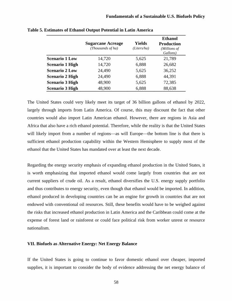
Fundamentals of a Sustainable U.S. Biofuels Policy
58
Table 5. Estimates of Ethanol Output Potential in Latin America
Sugarcane Acreage
(Thousands of ha) Yields
(Liters/ha)
Ethanol
Production (Millions of
Gallons)
Scenario 1 Low 14,720 5,625 21,789
Scenario 1 High 14,720 6,888 26,682
Scenario 2 Low 24,490 5,625 36,252
Scenario 2 High 24,490 6,888 44,391
Scenario 3 High 48,900 5,625 72,385
Scenario 3 High 48,900 6,888 88,638
The United States could very likely meet its target of 36 billion gallons of ethanol by 2022,
largely through imports from Latin America. Of course, this may discount the fact that other
countries would also import Latin American ethanol. However, there are regions in Asia and
Africa that also have a rich ethanol potential. Therefore, while the reality is that the United States
will likely import from a number of regions—as will Europe—the bottom line is that there is
sufficient ethanol production capability within the Western Hemisphere to supply most of the
ethanol that the United States has mandated over at least the next decade.
Regarding the energy security emphasis of expanding ethanol production in the United States, it
is worth emphasizing that imported ethanol would come largely from countries that are not
current suppliers of crude oil. As a result, ethanol diversifies the U.S. energy supply portfolio
and thus contributes to energy security, even though that ethanol would be imported. In addition,
ethanol produced in developing countries can be an engine for growth in countries that are not
endowed with conventional oil resources. Still, these benefits would have to be weighed against
the risks that increased ethanol production in Latin America and the Caribbean could come at the
expense of forest land or rainforest or could face political risk from worker unrest or resource
nationalism.
VII. Biofuels as Alternative Energy: Net Energy Balance
If the United States is going to continue to favor domestic ethanol over cheaper, imported
supplies, it is important to consider the body of evidence addressing the net energy balance of
Fundamentals of a Sustainable U.S. Biofuels Policy
59
domestically produced ethanol. Questions have arisen whether the energy required to plant,
produce, and transport ethanol from the U.S. Midwest is efficient or whether more fossil energy
is used in producing ethanol than is gained in new ethanol supplies.
Ethanol can be produced from a variety of feedstock. We focus on corn, which at present is the
basis of most U.S. production, and sugarcane, the basis of ethanol production in Brazil and
potentially many other countries. The production of ethanol requires the input of energy—
whether in the transportation fuel used to get biomaterials to the biorefineries or the
transportation fuel to carry the final product to market; in the production of fertilizers and
insecticides needed to enhance yields of the basic biomass; in the operation of the farm
machinery needed to prepare the soil, produce, and finally harvest the crop; or in the operation of
the biorefinery that converts the biomass to ethanol.
There has been a great deal of controversy over whether corn-based ethanol is a net contributor
to energy output. Energy balance is defined as the difference between how much energy a fuel
provides and how much energy it takes to create the fuel. For any alternative fuel, energy balance
is often used as a metric in determining the economic cost of replacing existing fuel sources with
the alternative. Studies on the energy balance of biofuels yield results ranging from positive to
negative, and there is much disagreement among specialists over the methodology of published,
peer-reviewed analysis.
The energy balance of a fuel varies considerably, based on its production process. Pimentel and
Patzek (2005) found a negative net energy balance for ethanol produced from a variety of
common U.S. feedstock, as summarized in Table 6. Interestingly, Pimentel and Patzek note that
the net energy balance of ethanol made from Brazilian sugarcane is also negative.
In contrast, Wessler (2006) found a positive net energy balance for ethanol from corn, soybeans,
and sunflowers and a less negative net energy balance for switchgrass and wood biomass-
generated fuel. His conclusions reflect his assumption that the energy inputs used in growing
feedstocks are not opportunity costs because the crops would be grown with or without an
ethanol industry.
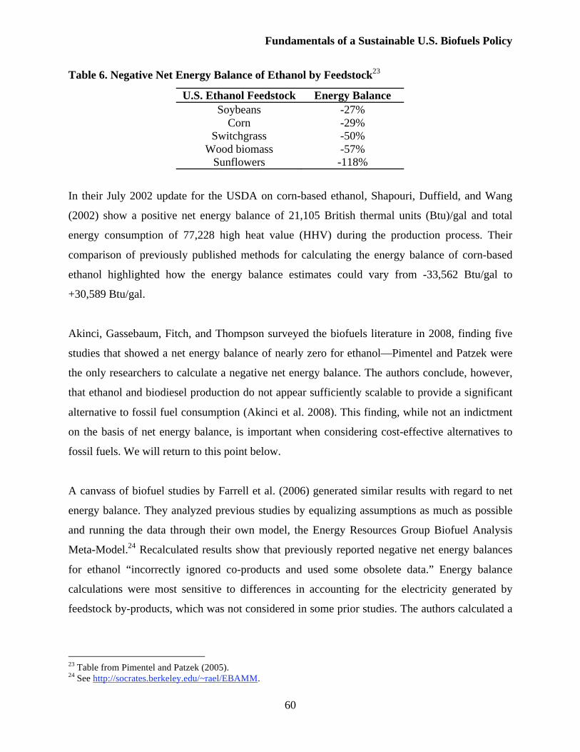
Fundamentals of a Sustainable U.S. Biofuels Policy
60
Table 6. Negative Net Energy Balance of Ethanol by Feedstock23
U.S. Ethanol Feedstock Energy Balance
Soybeans -27% Corn -29%
Switchgrass -50% Wood biomass -57%
Sunflowers -118%
In their July 2002 update for the USDA on corn-based ethanol, Shapouri, Duffield, and Wang
(2002) show a positive net energy balance of 21,105 British thermal units (Btu)/gal and total
energy consumption of 77,228 high heat value (HHV) during the production process. Their
comparison of previously published methods for calculating the energy balance of corn-based
ethanol highlighted how the energy balance estimates could vary from -33,562 Btu/gal to
+30,589 Btu/gal.
Akinci, Gassebaum, Fitch, and Thompson surveyed the biofuels literature in 2008, finding five
studies that showed a net energy balance of nearly zero for ethanol—Pimentel and Patzek were
the only researchers to calculate a negative net energy balance. The authors conclude, however,
that ethanol and biodiesel production do not appear sufficiently scalable to provide a significant
alternative to fossil fuel consumption (Akinci et al. 2008). This finding, while not an indictment
on the basis of net energy balance, is important when considering cost-effective alternatives to
fossil fuels. We will return to this point below.
A canvass of biofuel studies by Farrell et al. (2006) generated similar results with regard to net
energy balance. They analyzed previous studies by equalizing assumptions as much as possible
and running the data through their own model, the Energy Resources Group Biofuel Analysis
Meta-Model.24 Recalculated results show that previously reported negative net energy balances
for ethanol “incorrectly ignored co-products and used some obsolete data.” Energy balance
calculations were most sensitive to differences in accounting for the electricity generated by
feedstock by-products, which was not considered in some prior studies. The authors calculated a
23 Table from Pimentel and Patzek (2005). 24 See http://socrates.berkeley.edu/~rael/EBAMM.
Fundamentals of a Sustainable U.S. Biofuels Policy
61
net positive energy balance for corn-based ethanol of between 4 and 9 million joules/liter
(MJ/liter).25
While the research remains inconclusive at this point, it tends to point in the direction of saying
that there is a small but positive net energy contribution for corn-based ethanol with the ratio of
energy output:input in the range of 1.3 to 1.8. However, corn is a poor source of ethanol when
compared with sugarcane with its energy output:input ratio of 8.3.26 Dias de Oliveira puts the
ethanol advantage much lower, with the energy efficiency ratio for corn at 1.1 and for sugarcane
at 3.7. When the energy required to clean up residues left by ethanol are included, the ratios drop
to 0.7 and 1.3 respectively (Dias de Oliveira 2006).
Corn is a starch that must be converted to sugar before conversion to ethanol, while sugarcane
starts off as a sugar. In addition, sugarcane bagasse (the residue after the juice is extracted) can
be burned to produce electricity not only for the distillery but also for export to the energy grid.
Finally, as Dias de Oliveira (2006) pointed out, on a per hectare basis sugarcane produces ten
times the biomass as corn.
This measure of efficiency, while interesting and relevant in some cases, should not be the sole,
or even the most important, metric used to decide whether any particular source of ethanol is
desirable or not. Rather, the correct criterion for deciding which biomass is viable to produce
ethanol—or whether any form of ethanol itself is a viable substitute for gasoline—is to consider
the relative costs and benefits of various forms of ethanol and how they compare with gasoline in
terms of cost, environmental impact, and energy balance.
It is interesting to note that so much attention has been paid to the net energy balance of ethanol,
especially when compared with hydrogen—a fuel that was favored early in the administration of
President George W. Bush. The energy contained in hydrogen produced from natural gas is less
than that in the natural gas used, thus rendering hydrogen even less attractive in its energy
balance than ethanol (Morris 2005).
25 Note: 1 million joules = 947.8 BTU. 26 “Beyond Science: The Economics and Politics of Responding to Climate Change.” Conference report, Baker
Institute for Public Policy.
Fundamentals of a Sustainable U.S. Biofuels Policy
62
The focus on energy balance reflects a concern with technical efficiency—the relationship
between physical inputs and outputs. However, the cost effectiveness of converting one fuel to
another is an equally, if not more, important driving factor in a market-based system, and it is
this measure that should inform public policy on alternative fuels.
VIII. Biofuels as Alternative Energy: Some Environmental Issues27
We turn our attention in this section to a discussion of some environmental issues associated
with expanded use of biofuels.
Promoting the sustainable widespread use of biofuels requires careful consideration of the
potential environmental impacts of doing so. The environmental issues that give pause for
concern are related to surface and ground water impacts, greenhouse gas emissions and local air
pollution, and the impact of land use changes. Briefly:
• Recent research indicates that expanded use of ethanol can have deleterious effects on
water quality, which follow from increases in pesticide and fertilizer runoff. Moreover,
water use from irrigation is generally higher than the water demands that exist from
processing oil-based fuels and will increase along with greater demand for biofuels,
which can create issues related to water rights downstream of the irrigation site.
• With regard to leaks from underground storage, ethanol itself does not impose the most
significant risk. Rather, potential dangers arise when ethanol is blended with gasoline in
higher concentrations (greater than 10 percent by volume). Specifically, ethanol-blended
gasoline can increase the size of the plumes of harmful components in gasoline such as
benzene, toluene, ethylbenzene, and xylenes (BTEX), which can result in greater risk of
exposure.
• Overall, greenhouse gas (GHG) emissions for biofuels, once considered lower than those
for gasoline, are now uncertain due to land use changes and emissions of nitrous oxide
(N2O). It is also unclear whether local air pollution is greater or lower due to compounds
hazardous to human health from biofuels.
27 To read the full text of the environmental issues associated with expanded use of biofuels in U.S. transportation
fuel, refer to Appendix I of this report.
Fundamentals of a Sustainable U.S. Biofuels Policy
63
• The environmental impacts of cellulosic ethanol (produced from feedstock such as
switchgrass) tend to be smaller than those of corn-based ethanol, although there are even
more uncertainties because these biofuels have not yet been commercially produced.
Suggested fertilizer application rates vary widely. Water use theoretically could be zero,
but some growers may choose to irrigate switchgrass to increase yields. Finally,
excluding land use changes, GHG emissions are substantially lower, but certain land use
changes may make cellulosic ethanol worse than gasoline.
Chemical Uses and Agricultural Practices
Meeting the mandated increased production of biofuels will inevitably result in increased
agricultural activity, such as tilling more acres and higher agrichemical application. These
changes will lead to adverse environmental impacts that range from local groundwater
degradation to eutrophication of distant coastal waters. Runoff from nitrogen fertilizers results in
the most apparent example of eutrophication, the Gulf of Mexico’s “dead zone,” a large area of
low oxygen (hypoxia) near the mouth of the Mississippi River in which some organisms,
particularly those living near the sea bed, cannot survive, leading to limited biodiversity and an
altered ecosystem.
Annual row crops such as those typically used as biofuel feedstock are especially prone to cause
soil erosion and nutrient runoff to surface water, with corn having one of the highest nutrient
application rate and nutrient loading to surface waters. Marginal lands— which may require even
greater fertilizer application and may be more susceptible to erosion and runoff—will also be
pressed into agricultural service to meet the EISA mandate. This will create the potential for a
substantial increase in detrimental impacts to water quality.
Agrichemical runoff includes both fertilizers (nitrogen and phosphorous) and chemicals designed
to kill pests (herbicides, fungicides, and pesticides such as atrazine and alachlor for corn and
glycophosphate, primarily for soybeans). Nitrogen and phosphorous discharge are considered
some of the primary contributors to the hypoxic zone in the Gulf of Mexico, which covered over
20,000 km2 (7,700 mi2) in 2007. Hypoxic zones are oxygen-deficient waters, and although they
are a natural incident observed to have occurred throughout geologic time, the shallow coastal
Fundamentals of a Sustainable U.S. Biofuels Policy
64
hypoxic zone of the Gulf of Mexico has increased in size since the 1950s. This dead zone
damages fishery resources, which can experience a decrease in species diversity along with a
slump in yields. Marine species are affected by such factors as altered food supplies, forced
migration, habitat reduction, and increased susceptibility to predation.
It is difficult to assess the full impact of hypoxia on Gulf fisheries because insufficient data on
the effects of hypoxia on fisheries exists (Rabalais, Turner, and Wiseman 2002). However, the
consensus has been that hypoxia is a detrimental ecological effect of nutrient loading in the
Mississippi River Basin. Estimates for total annual freshwater costs from eutrophication are
between $105 to $160 million in the United Kingdom (Pretty et al. 2003) and approximately $2.2
billion for the United States (Dodds et al. 2009), but these calculations are uncertain and do not
attempt to price the impacts to saltwater areas such as the Gulf of Mexico.
Pesticides are toxic to humans as well as to other fauna. A 10-year (1992–2001) survey of U.S.
streams and groundwater showed that pesticides occurred in more than 50 percent of the wells
sampled in shallow groundwater and in 33 percent of deeper wells (U.S. Geological Survey
[USGS] 2006). Ninety-seven percent of stream waters in agricultural areas presented pesticide
compounds, and particularly high concentrations were found in the Corn Belt. The impact of
these agricultural pesticides on water quality continues to be studied and is often hotly debated,
but in a 2003 study, atrazine was implicated as an endocrine disruptor contributing to mutations
in frogs even at very low concentrations (Hayes et al. 2003). Since pesticides are usually found
as a mixture of compounds rather than individually, there is a potential for underestimating their
toxicity.
Application rates of agrichemicals vary widely among crops. Figure 10 presents the application
rates for nitrogen fertilizer and pesticides available for bioenergy crops in a manner that
normalizes the application rates to biofuel production potential. This metric is the most important
for comparisons of biofuels, and it is worth noting that sugarcane is among the lowest in terms of
agrichemical application. The actual application of fertilizer on a per-acre basis is similar for
sugarcane and corn, but sugarcane has a much higher net energy yield (we return to this latter
point in the next section).
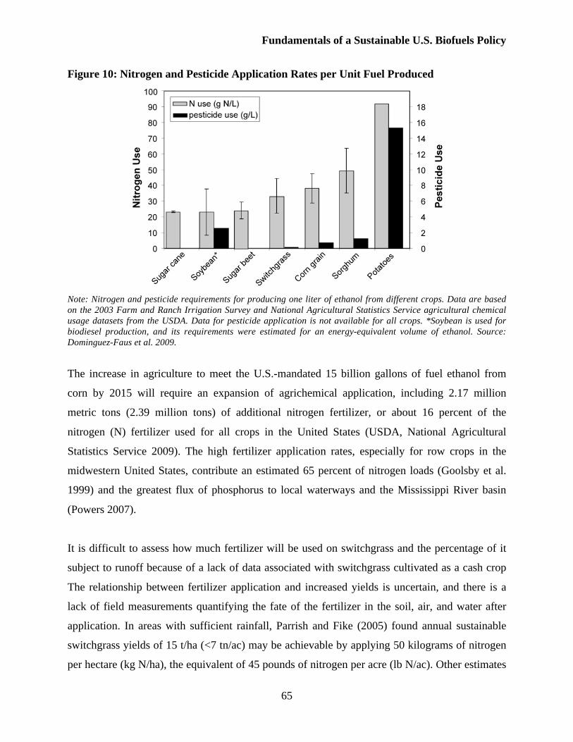
Fundamentals of a Sustainable U.S. Biofuels Policy
65
Figure 10: Nitrogen and Pesticide Application Rates per Unit Fuel Produced
Note: Nitrogen and pesticide requirements for producing one liter of ethanol from different crops. Data are based
on the 2003 Farm and Ranch Irrigation Survey and National Agricultural Statistics Service agricultural chemical
usage datasets from the USDA. Data for pesticide application is not available for all crops. *Soybean is used for
biodiesel production, and its requirements were estimated for an energy-equivalent volume of ethanol. Source:
Dominguez-Faus et al. 2009.
The increase in agriculture to meet the U.S.-mandated 15 billion gallons of fuel ethanol from
corn by 2015 will require an expansion of agrichemical application, including 2.17 million
metric tons (2.39 million tons) of additional nitrogen fertilizer, or about 16 percent of the
nitrogen (N) fertilizer used for all crops in the United States (USDA, National Agricultural
Statistics Service 2009). The high fertilizer application rates, especially for row crops in the
midwestern United States, contribute an estimated 65 percent of nitrogen loads (Goolsby et al.
1999) and the greatest flux of phosphorus to local waterways and the Mississippi River basin
(Powers 2007).
It is difficult to assess how much fertilizer will be used on switchgrass and the percentage of it
subject to runoff because of a lack of data associated with switchgrass cultivated as a cash crop
The relationship between fertilizer application and increased yields is uncertain, and there is a
lack of field measurements quantifying the fate of the fertilizer in the soil, air, and water after
application. In areas with sufficient rainfall, Parrish and Fike (2005) found annual sustainable
switchgrass yields of 15 t/ha (<7 tn/ac) may be achievable by applying 50 kilograms of nitrogen
per hectare (kg N/ha), the equivalent of 45 pounds of nitrogen per acre (lb N/ac). Other estimates
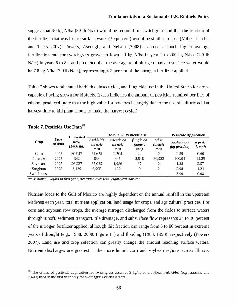
Fundamentals of a Sustainable U.S. Biofuels Policy
66
suggest that 90 kg N/ha (80 lb N/ac) would be required for switchgrass and that the fraction of
the fertilizer that was lost to surface water (30 percent) would be similar to corn (Miller, Landis,
and Theis 2007). Powers, Ascough, and Nelson (2008) assumed a much higher average
fertilization rate for switchgrass grown in Iowa—0 kg N/ha in year 1 to 260 kg N/ha (230 lb
N/ac) in years 6 to 8—and predicted that the average total nitrogen loads to surface water would
be 7.8 kg N/ha (7.0 lb N/ac), representing 4.2 percent of the nitrogen fertilizer applied.
Table 7 shows total annual herbicide, insecticide, and fungicide use in the United States for crops
capable of being grown for biofuels. It also indicates the amount of pesticide required per liter of
ethanol produced (note that the high value for potatoes is largely due to the use of sulfuric acid at
harvest time to kill plant shoots to make the harvest easier).
Table 7. Pesticide Use Data28
Total U.S. Pesticide Use Pesticide Application
Crop Year
of data
Harvested
area
(1000 ha)
herbicide
(metric
ton)
insecticide
(metric
ton)
fungicide
(metric
ton)
other
(metric
ton)
application
(kg pest./ha)
g pest./
L etoh
Corn 2005 30,947 71,625 2,204 42 0 2.39 0.66
Potatoes 2005 342 634 445 2,515 30,923 100.94 15.29
Soybeans 2005 26,237 35,085 1,086 87 0 1.38 2.57
Sorghum 2003 3,426 6,995 120 0 0 2.08 1.24
Switchgrass -- -- -- -- -- -- 3.00 0.08
** Assumed 3 kg/ha in first year, averaged over total eight-year harvest.
Nutrient loads to the Gulf of Mexico are highly dependent on the annual rainfall in the upstream
Midwest each year, total nutrient application, land usage for crops, and agricultural practices. For
corn and soybean row crops, the average nitrogen discharged from the fields to surface waters
through runoff, sediment transport, tile drainage, and subsurface flow represents 24 to 36 percent
of the nitrogen fertilizer applied, although this fraction can range from 5 to 80 percent in extreme
years of drought (e.g., 1988, 2000, Figure 11) and flooding (1983, 1993), respectively (Powers
2007). Land use and crop selection can greatly change the amount reaching surface waters.
Nutrient discharges are greatest in the more humid corn and soybean regions across Illinois,
28 The estimated pesticide application for switchgrass assumes 3 kg/ha of broadleaf herbicides (e.g., atrazine and
2,4-D) used in the first year only for switchgrass establishment.
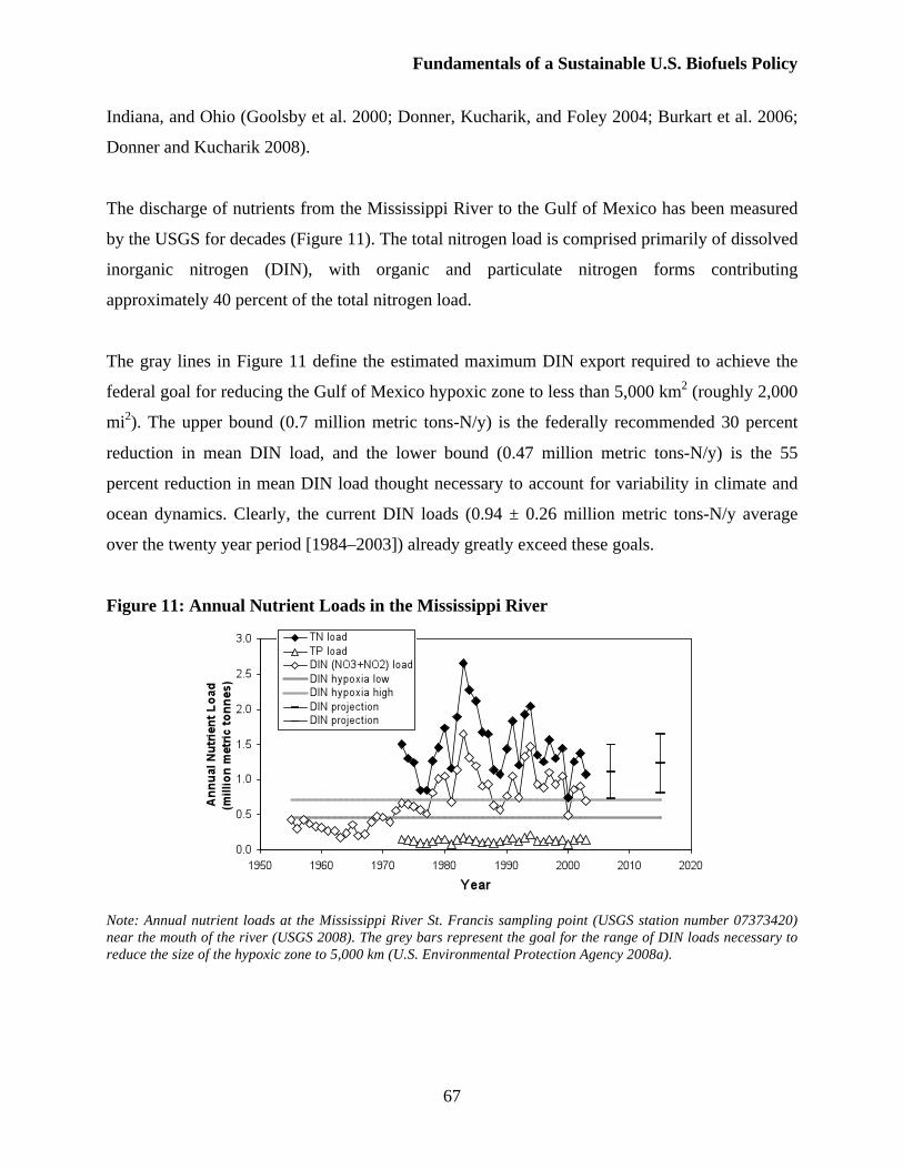
Fundamentals of a Sustainable U.S. Biofuels Policy
67
Indiana, and Ohio (Goolsby et al. 2000; Donner, Kucharik, and Foley 2004; Burkart et al. 2006;
Donner and Kucharik 2008).
The discharge of nutrients from the Mississippi River to the Gulf of Mexico has been measured
by the USGS for decades (Figure 11). The total nitrogen load is comprised primarily of dissolved
inorganic nitrogen (DIN), with organic and particulate nitrogen forms contributing
approximately 40 percent of the total nitrogen load.
The gray lines in Figure 11 define the estimated maximum DIN export required to achieve the
federal goal for reducing the Gulf of Mexico hypoxic zone to less than 5,000 km2 (roughly 2,000
mi2). The upper bound (0.7 million metric tons-N/y) is the federally recommended 30 percent
reduction in mean DIN load, and the lower bound (0.47 million metric tons-N/y) is the 55
percent reduction in mean DIN load thought necessary to account for variability in climate and
ocean dynamics. Clearly, the current DIN loads (0.94 ± 0.26 million metric tons-N/y average
over the twenty year period [1984–2003]) already greatly exceed these goals.
Figure 11: Annual Nutrient Loads in the Mississippi River
Note: Annual nutrient loads at the Mississippi River St. Francis sampling point (USGS station number 07373420)
near the mouth of the river (USGS 2008). The grey bars represent the goal for the range of DIN loads necessary to
reduce the size of the hypoxic zone to 5,000 km (U.S. Environmental Protection Agency 2008a).
Fundamentals of a Sustainable U.S. Biofuels Policy
68
Donner and Kucharik employed a rigorous agricultural and process-based dynamic ecosystem
model to predict the impact of increased corn production in the Midwest on nitrogen discharge to
the Gulf of Mexico (Donner 2003; Donner and Kucharik 2003; Donner, Kucharik, and Foley
2004; Donner and Kucharik 2008). The symbols included in Figure 11 for the year 2015 are their
estimates for the mean (±95 percent confidence interval) DIN exports that will result with
expanded production to meet the 15 billion gallons per year corn-based ethanol goals. They
predicted a 10 to 18 percent increase in DIN, further increasing the odds that these nitrogen loads
will exceed the target set without significant changes in agricultural management (Goolsby et al.
2000).
There are steps that can, and likely should, be taken to reduce the problems of nutrient runoff. A
variety of technological options can be used to reduce runoff, including contour farming,
terraced farmland, reduced nitrogen application, grassed waterways, restored wetlands, and
reduced tillage practices such as no-till or conservation tillage agriculture (Doering, Diaz-
Hermelo et al. 1999; Secchi et al. 2007). Secchi et al. (2007) analyzed the costs and effectiveness
of some of these methods for farms in Iowa, and it appears most cost-effective to focus attention
on reducing runoff from tile-drained land (Petrolia and Gowda 2006). From a more economic
perspective, nitrogen runoff would likely also be reduced with a price on nitrogen fertilizer or a
system of nitrogen runoff trading between point and nonpoint sources (Ribaudo, Heimlich, and
Peters 2005).
The presence of tile drainage is a very important factor in determining nutrient transport fluxes.
Tile drainage involves a network of clay, concrete, or perforated plastic subsurface pipes that
hasten removal of excess water, which in turn improves nutrient uptake of plant roots. A study
comparing tile-drained and nondrained soils in Iowa showed that the fraction of nitrogen
fertilizer lost to surface waters ranged from an average of 8 percent in nondrained fields to 36
percent in tile-drained fields (Powers, Ascough, and Nelson 2008). In the future, if tile drained
lands are used predominantly for growing crops that do not require significant nitrogen fertilizer
or those that are more effective at taking up the fertilizer, the nitrogen losses to surface water can
be reduced.
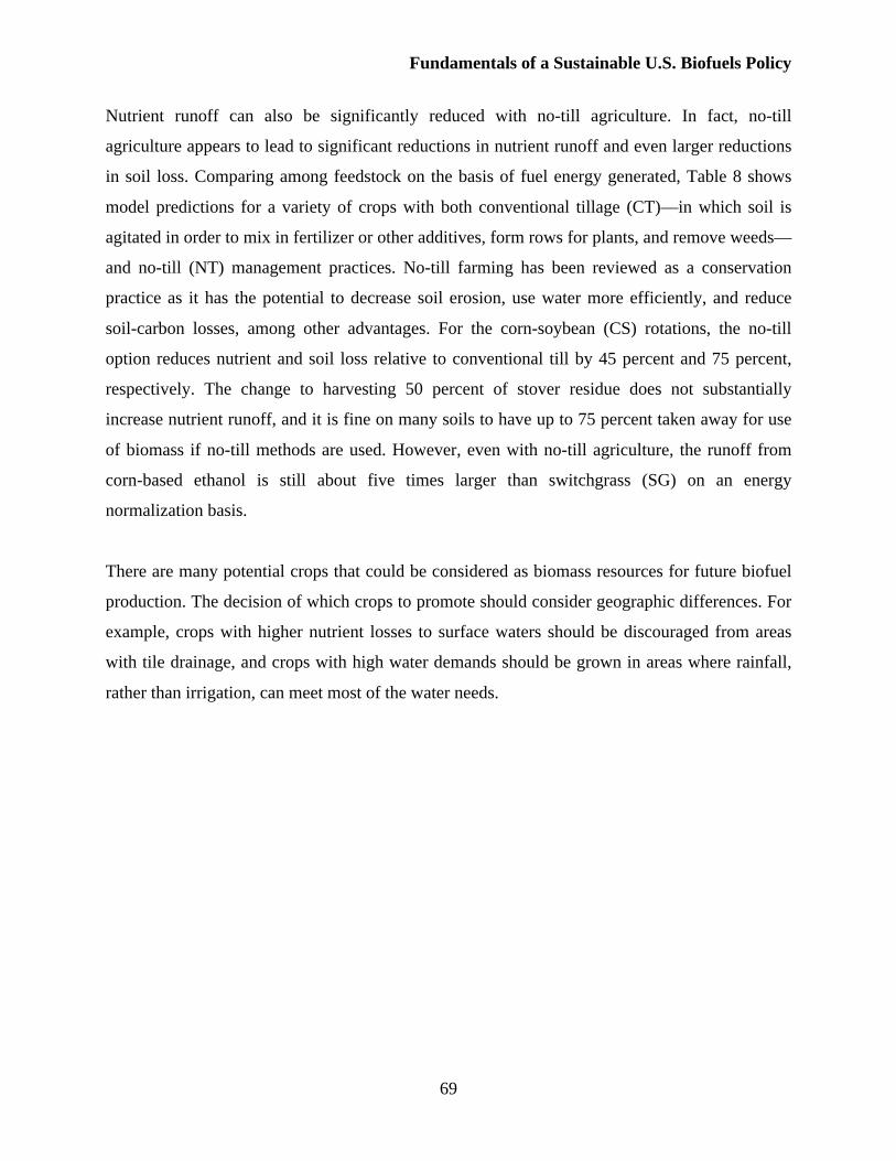
Fundamentals of a Sustainable U.S. Biofuels Policy
69
Nutrient runoff can also be significantly reduced with no-till agriculture. In fact, no-till
agriculture appears to lead to significant reductions in nutrient runoff and even larger reductions
in soil loss. Comparing among feedstock on the basis of fuel energy generated, Table 8 shows
model predictions for a variety of crops with both conventional tillage (CT)—in which soil is
agitated in order to mix in fertilizer or other additives, form rows for plants, and remove weeds—
and no-till (NT) management practices. No-till farming has been reviewed as a conservation
practice as it has the potential to decrease soil erosion, use water more efficiently, and reduce
soil-carbon losses, among other advantages. For the corn-soybean (CS) rotations, the no-till
option reduces nutrient and soil loss relative to conventional till by 45 percent and 75 percent,
respectively. The change to harvesting 50 percent of stover residue does not substantially
increase nutrient runoff, and it is fine on many soils to have up to 75 percent taken away for use
of biomass if no-till methods are used. However, even with no-till agriculture, the runoff from
corn-based ethanol is still about five times larger than switchgrass (SG) on an energy
normalization basis.
There are many potential crops that could be considered as biomass resources for future biofuel
production. The decision of which crops to promote should consider geographic differences. For
example, crops with higher nutrient losses to surface waters should be discouraged from areas
with tile drainage, and crops with high water demands should be grown in areas where rainfall,
rather than irrigation, can meet most of the water needs.
Fundamentals of a Sustainable U.S. Biofuels Policy
70
Table 8. Modeled Nutrient Losses and Soil Erosion for Energy Crop Scenarios when
Normalized by Energy Content29
g/MJ fuel g/MJ fuel t/MJ fuel
Summary TN/energy TP/energy soil/energy Corn (CSCT) 0.37 0.050 0.109 Corn (CSNT) 0.27 0.034 0.028 Soy (CSCT) 2.28 0.308 0.671 Soy (CSNT) 1.55 0.192 0.159
Stover 50% (CSNT) 0.028 0.004 0.010 SG 0.065 0.037 0.016
Notes: All values averaged over a 26-year period with soils and climate typical of eastern Iowa; CSCT/CSNT–corn
soybean rotation with conventional till/no till; Stover harvest of 50 percent of available stover as part of CSNT
rotation. Model assumes that no extra fertilizer is applied to replace the nutrient content of the harvested stover; SG
switchgrass with increasing fertilizer rates over the crop life. Model includes two consecutive 8-year cycles.
Such impressive reductions in nutrient runoff raise the question whether no-till agriculture
should be incentivized or even mandated. While pesticides are strictly regulated by the Federal
Insecticide, Fungicide, and Rodenticide Act (FIFRA) last amended in 1988, there are no
regulations on fertilizer application and storage. The USDA Natural Resources Conservation
Service (NRCS) has established nutrient management standards, which is a set of voluntary best
management practices regarding the amount, source, placement, form, and timing of the
application of nutrients (Dominguez-Faus et al. 2009).30 Biofuel production in no-till agriculture
is nearly identical to production when conventional techniques are used. Even absent expansion
of domestic ethanol production, these agricultural practices carry environmental benefits that
should be considered.
Water Demands of Biofuels from Selected Traditional Crops and Switchgrass
When discussing water use, it is important to differentiate between water withdrawals and water
consumption. Water withdrawals (water taken from a source) are more easily measured, but they
do not necessarily correspond with water consumption (water lost from the resource system that
will be unavailable for other uses). Part of the water withdrawn for a given purpose will be
consumed, while part of it will be returned to the system and available for reuse. Examples of
water consumption are evaporation losses from cooling towers in power generation and
29 Powers, Ascough et al. 2008. 30 These standards and potential regulations are under revision since research is still undergoing on the mechanisms
by which the chemicals applied to the fields can be transported to water bodies.
Fundamentals of a Sustainable U.S. Biofuels Policy
71
evapotranspiration losses from biophysical systems, such as agricultural systems. Different
economic activities have different impacts on both withdrawals and depletion of water. In the
United States, power generation is responsible for 39 percent of total national withdrawals, while
only for 3.3 percent of total national water consumption, whereas agriculture accounts for 40
percent of total water withdrawals and for as much as 80 percent of total water consumption
(Sandia National Laboratories 2006; Hutson et al. 2004; Gollehon and Quinby 2006). Any plans
that involve intensification of agriculture will have important effects on intensification of water
consumption. This is very relevant to biofuel policy because biofuel feedstock cultivation,
usually row-crop agriculture, is the most water intensive of the stages of biofuels production by
far. Water requirements for a typical sugarcane or corn ethanol refinery are around 2 to 10 liters
of water per liter of ethanol produced (National Research Council 2008), while consumption
(evapotranspiration) water requirements to produce enough feedstock to make one liter of
ethanol in the United States range from 500 to 5,000 liters, depending on what crop is used to
produce it.31 Water consumption of corn ethanol in the United States is 1,200 liters of water per
liter of ethanol (Lw/Le) (Figure 12).
In the United States, virtually all bioethanol (ethanol from biomass) currently produced is corn-
based. EISA mandates that more corn ethanol must be produced until reaching a cap of 15 billion
gallons (57 billion liters) annually by 2015. Meeting the mandated 15 billion gallons of fuel
ethanol from corn will require 44 percent of 2007 United States corn production,32 when corn
was planted on 93.6 million acres, or about 37.9 million hectares (USDA, National Agricultural
Statistics Service 2008). If the current proportion of irrigated corn (20 percent), is maintained
throughout the expansion, and assuming a national average withdrawal rate for corn ethanol of
566 Lw/Le (Figure 12), 6.3 trillion liters (1.7 trillion gallons) of irrigation water will be needed
31 Assuming a conservative volumetric water to ethanol ratio of 800 (e.g., for irrigated corn ethanol from Nebraska),
and that a car can drive 16 miles on one gallon of ethanol (or 2/3 of the mileage from gasoline), this represents about 50 gallons of water per mile driven (gwpm). To illustrate the variability of the water requirement as a function of the
crop used and where it is grown, this value could decrease to 23 gwpm for corn grown in Iowa, or increase to 90
gwpm if sorghum ethanol from Nebraska is used, or 115 gwpm if the sorghum is grown in Texas. 32 Assuming current ethanol yield efficiencies (387 liters of ethanol per metric ton of corn grain) based on the
biochemical transformation pathway of starches to ethanol.
Fundamentals of a Sustainable U.S. Biofuels Policy
72
for the corn used for ethanol, or about 3 percent of all irrigation water use in the U.S. in 2000.33
This is the equivalent of 1.25 times the total water withdrawals for all uses in the state of Iowa.
But this estimate assumes expansion will happen in the best land and water conditions like those
of much of the Corn Belt. The mandated ethanol expansion will not, however, be entirely met
with those optimal growth conditions. Expansion is, for now, occurring in the Midwest (National
Agricultural Statistics Service 2008), but while some midwestern regions can satisfy most of the
agricultural water requirements with rainfall (for example, in Ohio less than 1 percent of corn
grown is irrigated), other regions rely primarily on irrigation, such as in Nebraska, where 72
percent of corn grown is irrigated (Dominguez-Faus et al. 2009). Chiu, Walseth, and Suh (2009)
identified a general trend in which irrigation water needs for corn ethanol increase from the East
to the West and from the Midwest to the Southwest of the United States, which can be very
useful at evaluating regional water impacts associated with biofuel crop expansion.
This spatial variability makes it difficult to assess the potential for increased irrigation
requirements to exacerbate competition for water resources and create local water shortages. If
expansion occurs in less optimal areas, water demand will be higher. A comprehensive regional
analysis on this topic by Chiu, Walseth, and Suh (2009) shows that water appropriation by corn
ethanol in the United States in the past three years has increased 246 percent whereas corn
ethanol production has increased only 133 percent. They estimate that 6.1 trillion liters (1.6
trillion gallons) of water were necessary for the ethanol produced in 2008. By extrapolating this
trend, 10.9 trillion liters (2.9 trillion gallons) of water will be needed for the corn used to meet
the EISA goal of 15 billion gallons of ethanol in 2015. The new amount represents about 5.76
percent of total U.S. 2000 water irrigation withdrawals, or the equivalent to all withdrawals of
individual states such as Arizona, Kansas, or New York (Table 9).
33 Note that this figure only includes the water needed for the corn used in ethanol production, which is only
projected to be 44 percent of the total crop. Therefore, total water use for corn irrigation in the United States will be
roughly twice this figure.
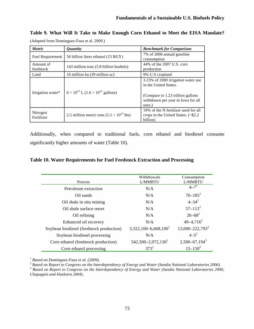
Fundamentals of a Sustainable U.S. Biofuels Policy
73
Table 9. What Will It Take to Make Enough Corn Ethanol to Meet the EISA Mandate?
(Adapted from Dominguez-Faus et al. 2009.)
Metric Quantity Benchmark for Comparison
Fuel Requirement 56 billion liters ethanol (15 BGY) 7% of 2006 annual gasoline
consumption Amount of
feedstock 143 million tons (5.8 billion bushels)
44% of the 2007 U.S. corn
production Land 16 million ha (39 million ac) 9% U.S cropland
Irrigation water* 6 1012 L (1.6 1012 gallons)
3.23% of 2000 irrigation water use
in the United States.
(Compare to 1.23 trillion gallons
withdrawn per year in Iowa for all
uses.)
Nitrogen
Fertilizer 2.5 million metric tons (5.5 1012 lbs)
19% of the N fertilizer used for all
crops in the United States. (~$2.2
billion)
Additionally, when compared to traditional fuels, corn ethanol and biodiesel consume
significantly higher amounts of water (Table 10).
Table 10. Water Requirements for Fuel Feedstock Extraction and Processing
Process
Withdrawals
L/MMBTU
Consumption
L/MMBTU
Petroleum extraction N/A 4–72
Oil sands N/A 76–1852
Oil shale in situ mining N/A 4–342
Oil shale surface retort N/A 57–1122
Oil refining N/A 26–682
Enhanced oil recovery N/A 49–4,7162
Soybean biodiesel (feedstock production) 3,322,100–6,668,1001 13,000–222,7933
Soybean biodiesel processing N/A 4–52
Corn ethanol (feedstock production) 542,500–2,072,1301 2,500–67,1943
Corn ethanol processing 3731 15–1502
1 Based on Dominguez-Faus et al. (2009).
2 Based on Report to Congress on the Interdependency of Energy and Water (Sandia National Laboratories 2006).
3 Based on Report to Congress on the Interdependency of Energy and Water (Sandia National Laboratories 2006;
Chapagain and Hoekstra 2004).
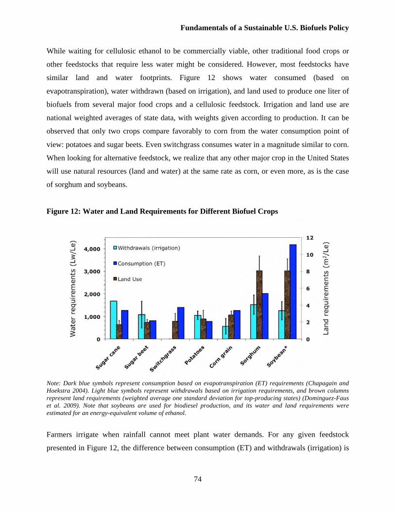
Fundamentals of a Sustainable U.S. Biofuels Policy
74
While waiting for cellulosic ethanol to be commercially viable, other traditional food crops or
other feedstocks that require less water might be considered. However, most feedstocks have
similar land and water footprints. Figure 12 shows water consumed (based on
evapotranspiration), water withdrawn (based on irrigation), and land used to produce one liter of
biofuels from several major food crops and a cellulosic feedstock. Irrigation and land use are
national weighted averages of state data, with weights given according to production. It can be
observed that only two crops compare favorably to corn from the water consumption point of
view: potatoes and sugar beets. Even switchgrass consumes water in a magnitude similar to corn.
When looking for alternative feedstock, we realize that any other major crop in the United States
will use natural resources (land and water) at the same rate as corn, or even more, as is the case
of sorghum and soybeans.
Figure 12: Water and Land Requirements for Different Biofuel Crops
Note: Dark blue symbols represent consumption based on evapotranspiration (ET) requirements (Chapagain and
Hoekstra 2004). Light blue symbols represent withdrawals based on irrigation requirements, and brown columns
represent land requirements (weighted average one standard deviation for top-producing states) (Dominguez-Faus
et al. 2009). Note that soybeans are used for biodiesel production, and its water and land requirements were
estimated for an energy-equivalent volume of ethanol.
Farmers irrigate when rainfall cannot meet plant water demands. For any given feedstock
presented in Figure 12, the difference between consumption (ET) and withdrawals (irrigation) is
Fundamentals of a Sustainable U.S. Biofuels Policy
75
indicative of the meteorological conditions of the region where it is grown. In that regard, the big
difference between consumption and withdrawals of corn and soybean only indicates that they
are mostly grown in the wet areas, such as most of the Midwest. Other crops that show a small
gap between consumption and withdrawals, or show a higher irrigation than consumption value,
such as sugarcane, sugar beets, and potatoes, will probably grow in areas where most of the
water that the plant needs comes from irrigation and not from rain.
Switchgrass theoretically requires no irrigation. It could be argued that it saves water, but since it
is similar in terms of consumption, its contribution to water conservation is just as limited as the
other crops. The real advantage of switchgrass is its greater resistance to droughts. Droughts are
abnormally dry conditions in which the water table drops temporarily. Switchgrass has a longer
rooting system than corn, which means that during a drought, it will be able to reach the deeper
water and survive until additional water arrives (rain or irrigation)—or at least survive longer
than corn, with its shorter roots. It can also be argued that switchgrass is not irrigated because it
has been relegated to marginal lands where growers have little interest in maximizing
productivity. However, when switchgrass is grown as a bioenergy crop and yields need to be
maximized, farmers can be expected to irrigate and fertilize.
Heightened Conflict over Water Resources
Increasing water use has the potential to exacerbate debates between states, localities, or farmers
about water rights, lead to negative environmental outcomes, and worsen the impacts of droughts
or more variable weather conditions. An example of a water rights argument occurred between
Nebraska and Kansas. Kansas farmers alleged that Nebraska farmers used 98 billion liters (26
billion gallons) more than their allotment of the Republican River in 2004 and 2005, as stipulated
in the agreement between the two states that the U.S. Supreme Court had approved in 2003
(Dominguez-Faus et al. 2009). Had farmers in Nebraska not used those 98 billion liters, they
would have needed to shut off irrigation to an estimated 485,000 hectares (1.2 million acres) of
farmland, or about 13 percent of the record 3.64 million hectares (9 million acres) planted in
Nebraska in 2007 and 2008. Additionally, increased use of groundwater resources, which
account for about 80 percent of irrigation in the Great Plains, can lead to spatial externalities in
which the uptake from water from one part of an underground aquifer can make it more
Fundamentals of a Sustainable U.S. Biofuels Policy
76
challenging or expensive for another user to extract water (Livingston and Garrido 2004;
Gollehon and Quinby 2006). This externality could lead to more localized disagreements or
problems.
In some locations, underground water sources are connected with surface wetlands that provide
habitats for waterfowl and other species (Livingston and Garrido 2004). If above-ground water
sources are used, certain minimum levels of water flow are needed to protect the habitat of fish
(Ward and Pulido-Velazquez 2008). Climate change has the potential to exacerbate these issues,
as extended periods of drought will put additional strain on the water supply.
Depending on the problem, water withdrawals and/or water consumption can be reduced, but
addressing one can potentially exacerbate the other. For instance, certain technologies such as
subsurface drip irrigation have been shown to reduce water withdrawals and often increase
productivity (Lamm and Trooien 2003). However, drip irrigation frequently increases net water
removal from water sources because less of the water returns to the original source through
surface runoff or deep penetration (Ward and Pulido-Velazquez 2008). Another option for
farmers is deficit irrigation, or the application of water below full requirements, but this
technique can reduce yields (Fereres and Soriano 2007).
Livingston and Garrido (2004) discuss the effectiveness of the four major administrative
approaches to managing groundwater—resource pricing, zoning, pumping quotas, and public
buyout—using theories about institutions and four case studies from the United States and Spain.
They find that it is important to establish rights to the water; one-time compensation to certain
users who agree to use less water can also be effective. In contrast, they note that raising the
price of water to encourage conservation is used infrequently. It can be difficult to set prices that
appropriately address the negative consequences of water use. Rather, disagreements over water
use are often mediated by trying to determine what the fair allocation of water is among various
users, and this can be more directly addressed with extraction limits.
The water used in biofuel processing is withdrawn from local sources and can lead to
disagreements in much the same way that irrigation can, even though it takes much less water to
Fundamentals of a Sustainable U.S. Biofuels Policy
77
turn biomass into ethanol than is needed to irrigate crops. For instance, the local water utility
refused to allow a plant proposed for Pipestone, Minn., by Cargill, Inc., because it was unable to
meet the 350 million gallon/year requirement of the proposed 100 million gallon/year plant. A
plant was approved in Grand Island, Neb., only after water use was reduced in an agricultural
area about 15 miles away (Keeney and Muller 2006). These water requirements may fall as
distilleries optimize their methods. One of many improvements under discussion is a facility that
could recycle wastewater or become a “zero process water discharge” plant that keeps and reuses
all wastewater (Marrone, Liberty, and Turton 2008).
Groundwater Pollution from Underground Storage Tanks
The increased use of ethanol nationwide increases the likelihood of leakage of ethanol into water
supplies and the environment, often when blended with gasoline in E-10 and E-85
concentrations. Underground storage tanks commonly found in gas stations and refineries are a
principal source of this contamination. These metal containers are prone to corrosion and
leaking, giving rise to a nationwide problem referred to as leaking underground storage tanks
(LUST). LUST is a quite common phenomenon, with over 479,000 confirmed releases, of which
over 377,000 have already been cleaned up (U.S. Environmental Protection Agency 2008a).
These releases can vary in magnitude from a few gallons to tens of thousands of gallons.
In order to assist remediation efforts, it is necessary to understand the unique dynamics and risks
associated with LUST that release fuel that includes ethanol. Research indicates that ethanol
itself is very unlikely to have strong direct adverse health and environmental consequences. In
this sense it is a substantial improvement over MTBE (methyl-tert-butyl ether)—a gasoline
additive that ethanol has largely replaced after MTBE was found to contaminate groundwater.
Ethanol degrades quickly in the environment through aerobic and anaerobic processes with a
surface water half-life of 6.5 to 26 hours, so there is little time for people to have the chance of
exposure (Ulrich 1999; Corseuil et al. 1998; Suflita and Mormile 1993; Howard et al. 1991).
Even if people were to consume ethanol in its denatured form, literature on ethanol metabolism
by humans indicates that environmental exposure to ethanol has minimal adverse human health
Fundamentals of a Sustainable U.S. Biofuels Policy
78
impacts with no symptoms observed below 1,000 parts per million (ppm) (American Council of
Governmental Industrial Hygienists 1991; Clayton and Clayton 1994).
Rather than the dangers of direct exposure to ethanol, the greater risk to human health comes
from the potential for BTEX mixed with ethanol to travel farther and be more difficult to degrade
(Da Silva and Alvarez 2002; Ruiz-Aguilar et al. 2002; Lovanh, Hun, and Alvarez 2002). Of the
BTEX hydrocarbons, benzene is potentially the most toxic and is known to be carcinogenic.
When more than 10 percent ethanol by volume is blended with gasoline (i.e., E-85), it inhibits
the degradation of dangerous compounds in gasoline known as BTEX (benzene, toluene,
ethylbenzene, and xylenes) that are directly damaging to human health. The BTEX-ethanol
mixture should travel farther (a phenomenon referred to as plume migration) and increase the
chances of exposure to more people, but overall impacts on human health are uncertain because
the amount of BTEX in the E-85 is generally lower and the overall life span of the plume is
shorter. In amounts of 10 percent ethanol or less, there are varying reports as to whether ethanol
will extend plume migration.
Releases of ethanol will most likely lead to some altered remediation approaches and possible
small-scale environmental damage. In terms of environmental impacts, ethanol can be toxic to
microorganisms, and the degradation of ethanol can lead to (1) hypoxic conditions, (2) a
potentially lower aqueous pH, and (3) the production of explosive methane and hydrogen gas.
A variety of factors inhibit the degradation of benzene in the presence of ethanol, which allows
the benzene to spread over a wider area. Benzene biodegrades at a much faster rate under aerobic
(with oxygen) rather than anaerobic (without oxygen) conditions, but the intense biodegradation
of ethanol depletes the oxygen in its plume path (Alvarez and Vogel 1995; Anderson et al. 1998;
Weiner and Lovley 1998a). Processes known as enzyme repression, catabolic repression, and
metabolic flux dilution also inhibit the degradation of benzene. Enzyme repression occurs when
the presence of the preferred substrate (ethanol) inhibits the production of the enzyme required to
degrade the target pollutant, BTEX (Duetz et al. 1994; Monod 1994; Hunt et al. 1997a; Corseuil
et al. 1998). Catabolic repression prevents microorganisms capable of degrading benzene from
utilizing their full potential (Madigan, Martinko, and Parker 2005), and metabolic flux dilution
Fundamentals of a Sustainable U.S. Biofuels Policy
79
involves carbon-limiting conditions when the utilization rate is due to the presence of ethanol
that is degraded simultaneously (Egli 1995; Lovanh and Alvarez 2004). Ethanol can also inhibit
anaerobic benzene degradation because ethanol depletes the available electron acceptors (sulfate,
manganese [IV], iron [III], and carbon dioxide) used in anaerobic degradation (Barker et al.
1992).
In contrast to the properties that slow the degradation of benzene, ethanol does promote the
growth of a wide variety of microbial populations, including those that can degrade BTEX
compounds (Alvarez 1999; Cápiro et al. 2008). The proliferation of these compounds would
result in faster BTEX degradation, but this positive effect of ethanol is likely to be offset by the
processes mentioned above.
Previous statistical studies show benzene plume elongation in the presence of ethanol. For
instance, benzene plumes resulting from regular versus E-10 gasoline spills show increased
benzene plume length (an average of 36 percent) when ethanol is blended with the gasoline
(Ruiz-Aguilar, O’Reilly, and Alvarez 2003). Laboratory experiments (Da Silva and Alvarez
2002; Lovanh, Hun, and Alvarez 2002; Lovanh and Alvarez 2004; Ruiz-Aguilar et al. 2002) and
modeling studies (Heermann and Powers 1996; McNab, Heermann, and Dooher 1999; Molson,
Barker, and Frind 2002; Gomez et al. 2008; Deeb et al. 2002) have also shown the elongation for
benzene, with changes ranging from 10 percent to 150 percent. However, these studies suffered
from many unknown factors influencing benzene plume length elongation, such as the age and
amount of spill, hydraulic conductivity, and soil porosity.
To address this uncertainty, a new mathematical model was recently developed to evaluate
plume elongation mechanisms and their relative importance (Gomez et al. 2008), and simulate
plume elongation as a function of ethanol content in gasoline (Gomez and Alvarez 2009).
Benzene plume lengths during the simulations showed elongations of ~60 percent for E-20 fuel
ethanol blends and of ~34 percent for E-85 blends. This modeling effort concluded that plume
elongation is primarily due to accelerated depletion of dissolved oxygen during ethanol
degradation, a decrease in the specific BTEX utilization in a noncompetitive but simultaneous
degradation of ethanol (known as metabolic flux dilution), and the repression of enzymes that
Fundamentals of a Sustainable U.S. Biofuels Policy
80
degrade BTEX in the presence of ethanol (a process known as catabolite repression). Catabolite
repression occurs because ethanol is a preferred source of carbon for the enzymes.
On the whole, this very likely plume elongation of BTEX could be detrimental to human health
from any given spill from a LUST. However, one positive sign is that the model shows a
significantly shorter life span of the benzene plume for blends with higher ethanol content: 17
years for regular gasoline, 15 years for E-10, 9 years for E-50 and 3 years for E-85. Increased
microbial activity in the presence of ethanol and a lower mass content of benzene due to dilution
account for the shorter life span.
The presence of ethanol in water sources can increase the risk for environmental damage. As
explained above, ethanol degradation lowers available oxygen, which can be damaging to marine
species living in the area of the fuel release. Ethanol also can be toxic to most microorganisms at
concentrations higher than 40,000 mg/l in water by disrupting the cellular permeability barrier
(Hunt et al. 1997a; Brusseau 1993; Ingram and Buttke 1984; Harold 1970). In the presence of
soil, microorganisms can find some protection, increasing effective toxicity values in the field;
microbial activity can occur at concentrations up to 100,000 mg/l (Araujo, Butler, and Mayfield
1998). Finally, if ethanol is degraded anaerobically, the pH of the groundwater can fall due to the
production of volatile fatty acids (VFAs) such as acetic, propionic, and butyric acid ((Lasko et al.
1997; Speece 1983). Anaerobic degradation can lead to accumulation of methane or hydrogen
gas, which may present a risk for explosive conditions with higher concentrations of ethanol,
although no instances of issues with methane have been reported. The presence of VFAs may
lead to a degradation of water quality if it leads to the reductive dissolution of metals and can
contribute undesirable taste and odor to the groundwater.
Remediation for LUST occurs at a state and local level (Sekely 2009). Certain states are
developing guidelines for how to deal with LUST with ethanol-blended fuels (Minnesota
Pollution Control Agency 2008). States that have printed guidelines do not believe E-10 fuel will
significantly alter the remediation process, and a document from the Maryland Department of the
Environment (2006) concludes, “The use of ethanol as a gasoline additive will likely have
Fundamentals of a Sustainable U.S. Biofuels Policy
81
minimal impact on the technology employed or the costs associated with groundwater or soil
remediation.”
Minnesota, a state with a significant number of E-85 pumps, is currently a leader in developing
guidelines for remediation of E-85 spills. Its interim document recognizes how the degradation
of BTEX can be delayed, leading to longer plume length, and it warns about the potential of
methane generation from ethanol degradation that could lead to explosive conditions and the
potential environmental consequences of low oxygen conditions (Minnesota Pollution Control
Agency 2008). On the whole, these recommendations fit relatively well with the analysis in this
report, but this work provides better quantitative assessments of the scope of the changes and a
better understanding of the processes that lead to various impacts.
Greenhouse Gas Emissions Associated with Biofuels Production and Use
Ethanol production leads to emission of GHGs and more localized air pollutants such as carbon
monoxide (CO) and nitrogen oxides (NOx). Older studies demonstrated that ethanol appeared to
emit less GHGs than conventional gasoline. However, thorough life cycle analysis presented in
more recent studies, however, that look at land use changes and the emissions of a less prevalent
but more potent GHG, nitrous oxide (N2O), question the overall reduction of GHGs from
biofuels. Moreover, even the benefits of cellulosic ethanol appear questionable once land use
changes are considered.
To make a proper assessment of the GHG emissions from biofuels, it is necessary to understand
that emissions are generated not only as a result of the combustion of the fuel, but also at each
phase of the fuel life cycle. Production, transport, and application of fertilizers, herbicides,
insecticides, feedstock transportation to distilleries, biofuels conversion, and distribution all
involve extensive use of fossil fuels that result in GHG emissions. These GHG emissions
primarily include carbon dioxide (CO2), methane (CH4), and nitrous oxide (N2O). The warming
potential per unit mass for each of these GHGs, which are usually expressed in CO2 equivalents,
are such that CH4 and N2O have GHG potentials that are 25 and 300 times of CO2, respectively
(Schlesinger 1997).
Fundamentals of a Sustainable U.S. Biofuels Policy
82
This conclusion that biofuels use is a carbon friendly alternative to conventional motor fuels is
now being challenged as researchers study potential land use changes and emissions of GHGs
other than CO2. In fact, research indicates that land use changes by themselves may put the
purported GHG benefits of all biofuels in doubt. On the other hand, ignoring land use changes
but fully accounting for N2O emissions would somewhat reduce but not eliminate the GHG
benefits of using cellulosic ethanol. Corn-based ethanol, however, may be another story. Crutzen
et al. (2007) argue that once N2O is considered in an assessment of life-cycle GHGs of corn-
based ethanol, there is likely no reduction in GHG emissions compared with conventional
gasoline.
With regard to land use changes, clearing forest and grassland in order to grow biofuel feedstock
results in release of carbon stored in plants and soils, either through decomposition or fire. It is
estimated that worldwide, each hectare of land converted for biofuel crops results in average
emissions of 351 mg of carbon dioxide equivalent. It is also estimated that the payback time for
such emissions is 167 years, assuming neutral tailpipe emissions from ethanol (Fargione et al.
2008; Searchinger et al. 2008). Increasing demand for biofuels has the undesirable potential to
further aggravate the already troublesome trend of clearing tropical forests in developed nations.
N2O emissions from crops come from the nitrogen (N) in the applied fertilizer. The emissions
occur both directly through nitrification and denitrification in the cropped soil and indirectly
when N is lost from the cropped soil as some form other than N2O (NOx, NH3, NO3) and later
converted to N2O off the farm. Estimates of in situ plus downstream N2O emissions range from 3
to 5 percent of the N fertilizer applied (Crutzen et al. 2007).34
Given the potential GHG impact of expanded fuel ethanol production, the stated goal of
enhancing energy security through using more biofuels must be juxtaposed with goals of
addressing climate change. More specifically, if we are to attempt to justify a renewable fuels
industry on the basis of lowering CO2 emissions as the goal of policy, this seems to call into
question that value of subsidizing biofuels energy production from traditional sources such as
34 It is estimated that croplands producing soy, wheat, and corn are responsible for about 68 percent of the total N2O
emissions in the United States (Mummey et al. 1998).
Fundamentals of a Sustainable U.S. Biofuels Policy
83
corn. The ethanol industry appears to emit GHGs per unit output in equal or greater amounts
when compared to the gasoline industry.
Localized Pollutant Effects Associated with Biofuels Production and Use
The effect of biofuels consumption on local air pollution is similarly uncertain. Pollutants such
as carbon monoxide (CO) and nitrogen oxides (NOx) that are associated with ethanol
combustion, for example, are directly harmful to human health. When compared to gasoline,
these emissions are lower at the tailpipe but higher when considering the life cycle of ethanol.
Thus, there may be some benefits to biofuels in terms of local air pollution in metropolitan areas
where tailpipe emissions are more likely to occur and affect residents in densely populated areas,
but the overall impacts are still uncertain.
As with gasoline, the burning of ethanol results in the emission of air pollutants that have
negative localized impacts. For some of these pollutants—carbon monoxide, nitrogen oxides,
particulate matter (PM), sulfur oxides (SOx), ozone (O3), volatile organic compounds (VOC),
and total hydrocarbons (THC)35—a life-cycle analysis shows that the emissions of all of these
pollutants increase with ethanol, and all but one (SOx) increase with biodiesel. However, unlike
GHGs, the impacts of these emissions depend on geography, so a reduction in air emissions in a
densely populated area from the burning of fuels can potentially be much more important than a
slight increase in life-cycle emissions.36 This follows since some proportion of the emissions
occur in less populated areas and 95 percent of the costs of air pollution are due to impacts on
human health (Rabl and Spadaro 2006). When compared with gasoline, tailpipe emissions are
uncertain for ethanol, although they look somewhat promising with three likely reductions (PM,
CO, THC) and only one increase and uncertainty (VOC and NOx). All tailpipe emissions from
biodiesel are better than conventional diesel fuel (see Table 11). It should be noted that in order
to have an estimate of such emissions as close as possible to the actual values, more
measurement experiments should be performed.
35 These six are regulated by the Clean Air Act (CAA), a bill last amended in 1990 with some minor changes since
then, that requires the U.S. Environmental Protection Agency (EPA) to set National Ambient Air Quality Standards (NAAQs) these common air pollutants. These six are known as “criteria pollutants” since the permissible levels of
pollution are based on health and/or environmental criteria. 36 The European ExternE project studied PM emission of less than 2.5 micrometers in France and determined that
the negative impact of a unit of particulate matter emitted in Paris is an order-of-magnitude worse than highway
emissions and two orders-of-magnitude worse than rural emissions (Rabl and Spadaro 2006).
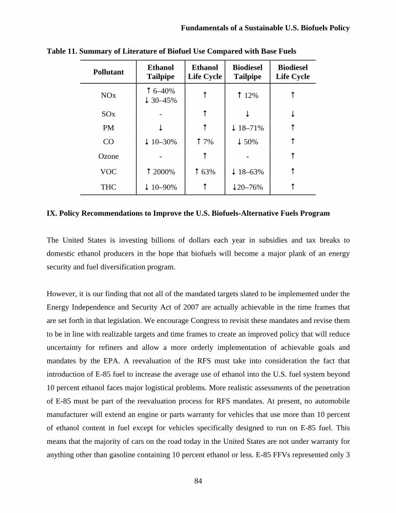
Fundamentals of a Sustainable U.S. Biofuels Policy
84
Table 11. Summary of Literature of Biofuel Use Compared with Base Fuels
Pollutant Ethanol
Tailpipe
Ethanol
Life Cycle
Biodiesel
Tailpipe
Biodiesel
Life Cycle
NOx 6–40%
30–45% 12%
SOx -
PM 18–71%
CO 10–30% 7% 50%
Ozone - -
VOC 2000% 63% 18–63%
THC 10–90% 20–76%
IX. Policy Recommendations to Improve the U.S. Biofuels-Alternative Fuels Program
The United States is investing billions of dollars each year in subsidies and tax breaks to
domestic ethanol producers in the hope that biofuels will become a major plank of an energy
security and fuel diversification program.
However, it is our finding that not all of the mandated targets slated to be implemented under the
Energy Independence and Security Act of 2007 are actually achievable in the time frames that
are set forth in that legislation. We encourage Congress to revisit these mandates and revise them
to be in line with realizable targets and time frames to create an improved policy that will reduce
uncertainty for refiners and allow a more orderly implementation of achievable goals and
mandates by the EPA. A reevaluation of the RFS must take into consideration the fact that
introduction of E-85 fuel to increase the average use of ethanol into the U.S. fuel system beyond
10 percent ethanol faces major logistical problems. More realistic assessments of the penetration
of E-85 must be part of the reevaluation process for RFS mandates. At present, no automobile
manufacturer will extend an engine or parts warranty for vehicles that use more than 10 percent
of ethanol content in fuel except for vehicles specifically designed to run on E-85 fuel. This
means that the majority of cars on the road today in the United States are not under warranty for
anything other than gasoline containing 10 percent ethanol or less. E-85 FFVs represented only 3
Fundamentals of a Sustainable U.S. Biofuels Policy
85
percent of the car fleet as of March 2009 and the availability of E-85 refueling stations is mainly
limited to only one region of the United States. The use of E-85 or FFVs is not likely to be
extensive enough to overcome the barriers to achieving the 2007 Energy Independence and
Security Act of 2007 mandates for U.S. ethanol market saturation. Moreover, existing mandated
targets for advanced biofuels are not currently achievable—commercially or scientifically—and
need to be revisited.
Furthermore, we note that ongoing implementation of current increases in feasible renewable
fuels production, such as corn-based ethanol, is coming with unintended detriments to the
environment. Because ethanol is easily degraded in the environment and human exposure to
ethanol itself presents minimal adverse health impacts, its role as a substitute for potentially
carcinogenic gasoline additive MTBE, on balance, represents a positive development. About 6
billion gallons per year (or 400,000 b/d) of ethanol are needed in the United States to replace
MTBE. However, the state and local environmental agencies responsible for site clean up must
take into consideration the fact that the addition of ethanol to gasoline beyond a 10 percent
concentration will impede the natural attenuation of BTEX in groundwater and soil, posing a
great risk for human exposure to these toxic constituents should the fuel leak from underground
storage tanks. The EPA can encourage these agencies to follow the lead of states like Minnesota,
which is already releasing guidelines for E-85 remediation.
We question the scale to which ethanol can enhance U.S. energy security by replacing oil-based
fuel and recommend that Congress order a cost-benefit analysis of the volume of renewable fuel
being added to the American transportation fuel system versus the cost per gallon to the
American taxpayer to achieve this marginal addition of non-fossil fuel based supply. We believe
that such an assessment would find that the extremely high costs of implementation of this
program would outweigh the indirect benefits to consumers of the small, marginal reductions in
U.S. oil imports.
We also recommend that Congress and the U.S. administration refrain from crediting corn-based
ethanol as receiving preferable treatment on the basis of its life-cycle greenhouse gas emissions
quality. There is no scientific consensus on the climate friendly nature of U.S. produced corn-
Fundamentals of a Sustainable U.S. Biofuels Policy
86
based ethanol and it is not justifiable to credit its use to reducing GHGs when compared to the
burning of traditional gasoline.
Increases in corn-based ethanol production in the U.S. Midwest could cause an increase in
detrimental environmental impacts, including exacerbating damage to ecosystems and fisheries
along the Mississippi River and in the Gulf of Mexico and creating water shortages in some areas
experiencing significant increases in fuel crop irrigation. Crops such as corn-based ethanol with
higher nutrient losses to surface waters should be discouraged from areas with tile drainage, and
crops with high water demands should be grown in areas where rainfall rather than irrigation can
meet most of the water needs. We recommend that Congress consider mandates that would
incentivize no-till agriculture as part of a sustainable renewable fuels program and that the
USDA’s NRCS revisit regulations on fertilizer application and storage.
Limitations in the economies of scale in ethanol production pose a significant barrier to
overcoming the logistical issues that block the widespread distribution of ethanol around the
United States, adding to the greenhouse gases emitted and conventional fuel burned in the
transportation of ethanol to end-use markets. A lifting of the $0.54/gal tariff on imported ethanol
from key countries in Central America, the Caribbean, and Latin America would allow coastal
areas of the United States to be more cheaply and sustainably supplied with ethanol while at the
same time help build trade and positive relations with important U.S. regional allies. We believe,
on balance, that the economic and geopolitical benefits of this trade with select regional suppliers
would outweigh any “energy security” costs associated with some larger percentage of U.S.
ethanol supplies arriving from foreign sources.
Imported ethanol from these regions is already making its way to U.S. shores through a variety
of loopholes, but at a higher cost. As discussed in this report, given the limitations of sustainable
production of U.S. domestic corn-based ethanol, tariff policies that block cheaper imports are
probably misguided. It is reasonable to ask if protective tariffs are meeting the goals for which
they were intended and if market participants—farmers, producers, blenders, or oil refiners—are
really reaping the actual profits from the tariffs.
Fundamentals of a Sustainable U.S. Biofuels Policy
87
Appendix I37
Introduction
Developing a sustainable national biofuels program requires careful consideration of logistical
concerns (e.g., suitable production and distribution infrastructure) and of unintended
environmental impacts. In this report we have reviewed the available scientific literature
concerning the environmental degradation associated with the increasing biofuel demand. In
particular, we have analyzed aspects of (1) air quality and greenhouse gas emissions, (2) ground
and surface water quality, and (3) impacts on water and land resources availability as a result of
increased biofuel demand.
Ethanol use as substitute for MTBE (methyl-tert-butyl ether) has significantly increased to meet
the need for renewable fuels and the requirements of the Clean Air Act. Extensive use of ethanol
in reformulated gasoline has increased its presence in gasoline- contaminated groundwater
aquifers, along with other fuel components such as benzene, toluene, ethylbenzene, and xylenes
(BTEX). A principal source of this contamination is underground storage tanks, a common
storage solution in gas stations and refineries. These metal containers are prone to corrosion and
leaking, giving rise to a nationwide problem: leaking underground storage tanks (LUST). Most
of the petroleum contamination that reaches groundwater aquifers originates from these leaking
storage tanks (Squillace et al. 1996), which has led to 479,000 confirmed cases of fuel release in
the United States since 1985 when the Environmental Protection Agency (EPA) opened its
Office of Underground Storage Tanks, with over 377,000 of them requiring some form of
remediation (U.S. EPA 2008). Although fuel spills from LUST can vary in magnitude from a
few gallons to tens of thousands of gallons (Nebraska Department of Environmental Quality
2005), the majority have constant low volume leaks that are hard to detect and could be present
for many years before remedial action is taken. Dakhel et al. (2003) performed field experiments
with small ethanol releases that indicate that groundwater impacts in these cases should be
minimal. The effects of large ethanol releases from LUST have been largely unstudied (Zhang et
37 Contributions by Pedro J. Alvarez, Joel G. Burken, Marcelo Dias de Oliveira, Rosa Dominguez-Faus, Diego E.
Gomez, and Susan E. Powers.
Fundamentals of a Sustainable U.S. Biofuels Policy
88
al. 2006). We will try to shed some light on this issue by presenting the direct and indirect
environmental implications of ethanol in groundwater. These implications on health and the
environment will be summarized, in the context of ethanol’s use as a fuel additive and its
impacts on groundwater contaminant transport.
Surface water quality is primarily affected by agrichemical (pesticides and fertilizer) runoff. The
most prominent effect is known as eutrophication (high levels of nutrients) of waters due to
fertilizer loss from agricultural fields. Eutrophication results in algal blooms. When algae die and
decay, it consumes oxygen dissolved in water, depleting it to levels as low as 2 mg/L, down from
the regular levels around 8 mg/L. Under the low oxygen conditions, scientifically referred as
hypoxia, life cannot be sustained. Areas undergoing this phenomenon have been called “dead
zones.” In the United States, the most famous dead zone is in the Gulf of Mexico, around the
Mississippi River delta, which receives high nutrient loads from agricultural activity upstream in
the Mississippi River basin. For this report, we have searched the scientific literature to identify
to what extent energy crops and various agricultural practices have contributed to hypoxia in the
Gulf of Mexico.
Another group of agrichemicals of concern are pesticides, since they are toxic to humans as well
as to other fauna. A 10-year (1992–2001) survey of streams and groundwater showed that
pesticides occurred in more that 50 percent of the wells sampled in shallow groundwater and in
33 percent of deeper wells. Ninety-seven percent of stream waters in agricultural areas presented
pesticide compounds; particularly high concentrations were found in the Corn Belt. Since
pesticides are usually found as a mixture of compounds, rather than individually, there is a
potential for underestimating their toxicity. Pesticide use is strictly regulated by the Federal
Insecticide, Fungicide, and Rodenticide Act (FIFRA), last amended in 1988. While there are no
regulations on fertilizer application and storage, the U.S. Department of Agriculture (USDA)
Natural Resources Conservation Service (NRCS) has established nutrient management standards,
which is a set of voluntary best management practices regarding the amount, source, placement,
form, and timing of the application of nutrients (Dominguez-Faus et al. 2009). These standards
and potential regulations are under revision, since research is still ongoing on the mechanisms by
which the chemicals applied to the fields can be transported to water bodies. For example,
Fundamentals of a Sustainable U.S. Biofuels Policy
89
chemicals can be transported attached to sediment in a water stream. Crop residues (cellulosic
material) protect the soil surface from the erosive effects of wind and rainfall, limiting the
amount of sediment that leaves the field. Therefore, removal of these residues can have
detrimental effects, increasing the final amount of chemicals reaching water bodies. In the
following section, we will review the fertilizers and pesticide requirements of several crops
considered for biofuel production, as well as summarize the findings of peer-reviewed studies on
the effect of removal of agricultural residue and till practices on water quality.
A final issue that has not received deserved attention is that of the water and land resources
demand for biofuels production. Forecasting future demand for such natural resources and
comparing them to available resources is a difficult task due to the many sources of uncertainty
surrounding those matters. Water and land requirements of biofuels will depend on what
feedstock is used, as well as where the feedstock is grown. Additional temporal variability of
climate plays a key role in forecasting the intensity of use of these resources, as well as its
availability (think of droughts). Changes in agricultural irrigation techniques that might come
through regulation or by choice, biotechnology advances, such as improvement of crop yields,
and conversion technology changes can alter the final value of overall land and water
requirements. The high number of variables suggest that the proper method for this analysis is
through the generation of possible future case scenarios. Unfortunately, these issues have not
been addressed by many scientists. In this report, we show what is probably the only scenario
constructed to date: a baseline scenario using current statistics, current state-of-the-art
technology, and current biofuel projections of the Energy Independence and Security Act (EISA)
of 2007, as constructed by researchers at Rice University. Ongoing research at Rice is
developing alternative scenarios, using an agricultural-climatic model combined with multiple
potential technological, political, and climatic changes.
Current State of Knowledge
1. Groundwater Pollution from Underground Storage Tanks
The main points of this analysis are:
• Ethanol is easily degraded in the environment and has a relatively short half-life (time
Fundamentals of a Sustainable U.S. Biofuels Policy
90
necessary for its concentration to be reduced to one-half of the original value) compared
to other constituents of concern in gasoline, such as BTEX and MTBE;
• Human exposure to fuel ethanol is not expected to be significant due to its short life in
the environment;
• Ethanol metabolism by ingestion into the human body and its related health effects
indicate that environmental exposures to ethanol on humans have minimal adverse health
impacts;
• Ethanol can directly hinder the biodegradation and natural attenuation of BTEX, leading
to increases in plume lengths and a higher likelihood of BTEX reaching receptors;
• Ethanol can change the growth and distribution of microbes, stimulating the proliferation
of microbial populations that degrade it, as well as BTEX degraders that fortuitously
grow on ethanol. This response to changes in oxygen and substrate availability can offset,
but not overcome, the mechanisms that hinder BTEX degradation activity at the
individual cell level. These include catabolite repression, which is defined as the
repression of inducible enzymes that degrade the target pollutant (e.g., BTEX) by the
presence of a preferred carbon source (e.g., ethanol), and metabolic flux dilution, which
is defined as a decrease in the specific BTEX utilization rate due to noncompetitive
inhibition when ethanol is present;
• The rate and metabolic end products of ethanol degradation vary depending on the
amount and concentration (E-10 vs. E-85) at the release site. This, in turn, determines the
type of end products at a receptor site;
• The released ethanol-rich phase is lighter than water and may concentrate in the source
zone at the water table interface. There, it would decrease the surface tension and
facilitate spreading through the capillary zone. As ethanol becomes diluted, the cosolvent
effect decreases and hydrocarbons come out of solution (phase-separation), creating a
residual nonaqueous phase liquid (NAPL) lens at the water table interface that serves as a
source of long-term groundwater contamination;
• Since ethanol is infinitely soluble in water, ethanol separates from the NAPL, dissolves
and is carried with the groundwater and rapidly begins biodegradation. For most releases
of E-10, ethanol rapidly biodegrades both aerobically (with oxygen) or anaerobically
(without oxygen) near the release site, with most plumes migrating more slowly and
Fundamentals of a Sustainable U.S. Biofuels Policy
91
disappearing more rapidly than BTEX plumes (1 to 2 years);
• Complete aerobic biodegradation of ethanol produces CO2 and water (acetaldehyde and
acetic acid [vinegar] as intermediates). This process consumes the oxygen in the surface
soils and potentially the subsurface aquifer. The more ethanol released, the more oxygen
consumed;
• Anaerobic biodegradation of ethanol begins when oxygen has been depleted from the
surface soils or when ethanol migrates into an oxygen-deprived zone in the subsurface.
Anaerobic biodegradation depletes these regions of electron acceptors (sulfates, nitrates,
iron, and manganese) and can lead to the accumulation of acetic acid, methane, and
hydrogen gas; and
• Ethanol may also act as a cosolvent if present in groundwater at concentrations greater
than 10,000 mg/L, increasing BTEX dissolution and mobility.
Direct health and environmental effects of ethanol releases in the environment are very unlikely
to have strong adverse consequences. This is mainly due to the fact that: (1) fast degradation of
ethanol, through aerobic and anaerobic processes, readily occurs in the environment (Ulrich
1999; Corseuil et al. 1998; Suflita and Mormile 1993); (2) due to its fast degradation and short
life in the environment, exposure of humans to toxic ethanol levels is not expected (Armstrong
2000); (3) literature on ethanol metabolism by humans, and the related health effects of ethanol
ingestion, indicate that environmental exposures to ethanol have a minimal adverse health
impact, with no symptoms observed below 1000 ppm (American Conference of Governmental
Industrial Hygienists [ACGIH] 1991; Clayton and Clayton 1994); (4) the human body
metabolizes and eliminates ethanol very quickly (Pohorecky and Brick 1987; Holford 1987); and
(5) ethanol is not persistent in the environment—it has a surface water half-life of 6.5 to 26 hours
(Howard et al. 1991).
On the other hand, ethanol has the potential to affect the natural attenuation and transport
processes of other target pollutants, like BTEX. The preferential biodegradation of ethanol and
associated accelerated depletion of dissolved oxygen and nutrients in aquifers may hinder BTEX
degradation. Decreased natural attenuation would, in turn, increase the length of BTEX plumes,
which raises a concern for increased down-gradient exposure (Da Silva and Alvarez 2002; Ruiz-
Fundamentals of a Sustainable U.S. Biofuels Policy
92
Aguilar et al. 2002; Lovanh, Hun, and Alvarez 2002). A statistical study of benzene plumes
resulting from regular versus E-10 (10 percent v/v ethanol/gasoline) gasoline spills shows an
average 36 percent increase in benzene plume length when ethanol is blended with the gasoline.
(Ruiz-Aguilar, O’Reilly, and Alvarez 2003). Laboratory experiments (Da Silva and Alvarez
2002; Lovanh, Hun, and Alvarez 2002; Lovanh and Alvarez 2004; Ruiz-Aguilar et al. 2002) and
modeling studies (Heermann and Powers 1996; McNab, Heermann, and Dooher 1999; Molson,
Barker, and Frind 2002; Gomez et al. 2008; Deeb et al. 2002) have also shown this elongation
for benzene, with changes ranging from 10 percent to 150 percent. This is particularly important
as benzene is potentially the most toxic of the BTEX hydrocarbons, and its presence in gasoline-
contaminated sites often dictates the need for remediation.
Many unknown factors influencing benzene plume length elongation remain, such as the age and
amount of spill, hydraulic conductivity, soil porosity, redox conditions, etc. As a result, there is
still considerable uncertainty regarding the magnitude and importance of the BTEX plume
elongating effects of ethanol. To address this uncertainty, a new mathematical model was
recently developed to evaluate plume elongation mechanisms and their relative importance
(Gomez et al. 2008), and to simulate plume elongation as a function of ethanol content in
gasoline (Gomez and Alvarez 2009). This modeling effort concluded that plume elongation is
primarily due to accelerated depletion of dissolved oxygen during ethanol degradation, and to a
decrease in the specific rate of benzene utilization resulting from metabolic flux dilution and
catabolite repression. Benzene plume lengths during the simulations showed elongations of ~60
percent for E-20 fuel ethanol blends and of ~34 percent for E-85 blends. Life span of the plume
was also significantly shorter for blends with higher ethanol content: 17 years for regular
gasoline, 15 years for E-10, nine years for E50 and three years for E-85. Increased microbial
activity due to the presence of ethanol, as well as lower mass content of benzene on the blends
due to dilution, account for the increased natural attenuation potential of higher ethanol blends.
Effect on the Unsaturated Zone
Ethanol can exert cosolvent effects that influence blended gasoline migration in the unsaturated
zone. First, reduced surface and interfacial tension due to ethanol results in a more complete
drainage of gasoline, leaving less residual chemicals entrapped in the unsaturated zone. Second,
Fundamentals of a Sustainable U.S. Biofuels Policy
93
a significant fraction of ethanol partitions and is retained by residual water in the capillary zone.
As this residual ethanol filters into the lower gasoline pool, it creates a nonuniform distribution
of ethanol on the light nonaqueous phase liquids (LNAPL) pool. This heterogeneous LNAPL
lens complicates the calculation and behavior of BTEX dissolution from the source. Finally, the
infiltration rate of residual ethanol toward the capillary fringe and the gasoline pool is limited by
the increased viscosity and, therefore, reduced unsaturated hydraulic conductivity of this phase
(Powers and McDowell 2001c). Another important property of ethanol is that in high
concentrations it partitions from fuel ethanol blends due to its higher buoyancy. This leads to a
phase separation and accumulation of ethanol on the capillary fringe, resulting in lower
groundwater concentrations near the source than would be expected if ethanol were considered
completely miscible (Cápiro et al. 2007).
Enzyme Induction and Repression
Easily degraded substrates, like ethanol, are often preferentially degraded by microorganisms
over more important target contaminants like benzene. One of the mechanisms for this is enzyme
repression, where the presence of the preferred substrate inhibits the production of the enzyme
required to degrade the target pollutant (Duetz et al. 1994; Monod 1949). This repression of
benzene-degrading enzymes in the presence of ethanol was reported by Hunt et al. (1997a)
during aerobic degradation experiments where benzene degradation was delayed. Furthermore,
microcosm studies by Corseuil et al. (1998) indicate that this mechanism might lead to slower in
situ BTEX biodegradation. This mechanism, known as catabolic repression, prevents
microorganisms capable of degrading benzene from utilizing their full potential, hindering
BTEX degradation and natural attenuation (Madigan, Martinko, and Parker 2005).
Other studies also point to carbon-limiting conditions as responsible for multi-substrate
utilization (Egli 1995), where a decrease in the specific benzene utilization rate is due to the
presence of ethanol, which is degraded simultaneously, a phenomenon also known as metabolic
flux dilution (Lovanh and Alvarez 2004).
Stimulation of Microbial Growth
One of the advantages of ethanol is that it promotes the growth of a wide variety of microbial
populations, including those that can degrade BTEX compounds (Alvarez 1999; Cápiro et al.
Fundamentals of a Sustainable U.S. Biofuels Policy
94
2008). Proliferation of BTEX degraders on ethanol (also known as fortuitous growth) would
result in faster BTEX degradation rates. Unfortunately, this positive effect of ethanol is likely to
be offset by its preferential degradation through the previously mentioned catabolic repression
and metabolic flux dilution. Ethanol degrading enzymes are associated with central metabolic
pathways, which can be utilized by many species that cannot degrade BTEX. Furthermore,
favorable thermodynamics lead to faster microbial growth on ethanol than on BTEX compounds,
with an increase in maximum specific growth rate of ~45 percent (Hunt 1999; McCarty 1969).
The overall result of these processes is a significant increase in BTEX degrading microbial
populations due to ethanol presence. However, ethanol can stimulate the growth of other bacteria
faster than BTEX degraders, which decreases their relative abundance (Da Silva and Alvarez
2002; Cápiro et al. 2007), a phenomenon known as genotypic dilution.
Microbial Toxicity of Ethanol
Ethanol has been shown to have high concentration toxicity values. Several sources report an
EC50 concentration (when microbial activity has been reduced by 50 percent of its maximum)
between 31,000 mg/L and 57,000 mg/L (Dutka and Kwan 1981). Ethanol concentrations higher
than 40,000 mg/L are toxic to most microorganisms, as shown during aerobic degradation
experiments reported by Hunt et al. (1997a). Ethanol is toxic to microorganisms through
disruption of the cellular permeability barrier (Brusseau 1993; Ingram and Buttke 1984; Harold
1970). In the presence of soil, microorganisms can find some protection, increasing effective
toxicity values in the field. Microbial activity can occur at concentrations up to 100,000 mg/L
(Araujo et al. 1998). The majority of microorganisms have toxicity values to ethanol in the range
of 10,000 to 100,000 mg/L.
Depletion of Nutrients and Electron Acceptors
Compared to BTEX and other gasoline components, ethanol exerts a significantly higher
biochemical oxygen demand in groundwater. This results in an accelerated consumption of
dissolved oxygen within the ethanol plume (Corseuil et al. 1998). Fast oxygen depletion hinders
aerobic BTEX degradation, and particularly of benzene, as it degrades at a much slower rate
under anaerobic conditions (Alvarez and Vogel 1995; Anderson et al. 1998; Weiner and Lovley
1998a). Anaerobic degradation of BTEX is also affected. Ethanol can be anaerobically degraded
Fundamentals of a Sustainable U.S. Biofuels Policy
95
under most common electron-acceptor conditions and this will lead to the depletion of other
important dissolved electron acceptors (i.e., ferric iron). Field studies were conducted by Barker
et al. (1992) using methanol, which presents environmental impacts similar to those of ethanol.
These studies involved releasing controlled amounts of BTEX and methanol mixtures. The
experiment showed, over the course of 476 days, that BTEX degradation is hindered by the
presence of methanol in the gasoline plume.
Accumulation of Volatile Fatty Acids
Ethanol degradation by mixed anaerobic cultures can result in the production of volatile fatty
acids (VFAs) (acetic, propionic, and butyric acid), which can accumulate and decrease the
groundwater pH (Lasko et al. 1997; Speece 1983) and contribute undesirable taste and odor to
the groundwater. This change in site conditions can also adversely affect some microbial
populations that perform BTEX natural attenuation. Methanogens can be inhibited by pH lower
than 6 (McCarty 1964), resulting in lower degradation rates of BTEX under such conditions. It is
not known if VFAs would accumulate in the field to the levels required to significantly decrease
the pH, inhibit microbial growth, and result in decreased natural attenuation rates. These effects
are likely to vary locally and be specific to site characteristic. Another potential impact of this
anaerobic souring effect is the reductive dissolution of metals that can further contribute to water
quality degradation.
Impact of Microbial Processes on Aquifer Permeability
Microbial growth is highly stimulated by ethanol’s presence. This enhanced microbial growth
could affect the hydrodynamic properties of the aquifer through the formation of biofilm and
microbial cell aggregates that can reduce the available pore space and become a potential
clogging mechanism (Taylor and Jaffe 1990; Vandevivere and Baveye 1992). Microorganisms
could also affect aquifer permeability by increasing mineral dissolution (for example, CaCO3)
and precipitation (for example, FeS). These opposing processes could affect soil pore space,
affecting the available area for contaminant sorption, thus affecting hydraulic conductivity and
darcy velocity, among other properties. However, laboratory column studies suggest that such
effects are minimal (Da Silva and Alvarez 2002).
Fundamentals of a Sustainable U.S. Biofuels Policy
96
Sorption and Cosolvency
Ethanol can have two effects on BTEX concentrations due to cosolvency effects. First, the
presence of ethanol in the water phase can decrease sorption-related retardation and is likely to
increase BTEX plume lengths. The effect of a cosolvent on BTEX has been described by Rao et
al. (1985). Cosolvent effects on sorption at ethanol concentrations expected from gasohol spills
should be minor, as shown by Powers (2001) and model simulations (Gomez et al. 2008).
The second effect is how ethanol can change the equilibrium partitioning of BTEX compounds
between the LNAPL phase and the water phase, which would have a direct impact on dissolution
rates of BTEX from spills into the ground, and pore water and the resulting plume
concentrations. Batch-equilibrium experiments were performed by Heermann and Powers (1998)
and compared with three mathematical models. Results of these experiences show an overall
increase in partition coefficients as a function of increasing ethanol content in the aqueous phase.
Heermann and Powers developed a model to predict BTEX concentrations using a linear
relationship for low ethanol volume fractions and a log-linear model for higher concentrations,
which showed that changes in gasoline-water partition due to ethanol can be significant.
Overall, although ethanol itself does not present a significant risk associated with drinking water
quality (other than perhaps to pregnant women if drunk in excess), its presence in contaminated
groundwater is likely to hinder the natural attenuation of hydrocarbons and elongate benzene
plumes, which represents a higher risk of cancer due to down-gradient exposure. Based on the
statistical field studies of Ruiz-Aguilar, O’Reilly, and Alvarez (2003), and the previous
laboratory and simulation studies (Da Silva and Alvarez 2002; Lovanh, Hun, and Alvarez 2002;
Lovanh and Alvarez 2004; Ruiz-Aguilar et al. 2002; Heermann and Powers 1996; McNab,
Heermann, and Dooher 1999; Molson, Barker, and Frind 2002; Gomez et al. 2008, Deeb et al.
2002) BTEX plume elongation is expected in the range of 35 percent to 55 percent when ethanol
is present. For an average benzene plume of 200 ft, this would mean a length of 270–310 ft under
the influence of ethanol. Values in this range have been shown in recent E-10 fuel simulation
studies by Gomez et al. (2008). This is a significant increase of 70 to 80 ft over the regular
gasoline baseline.
Fundamentals of a Sustainable U.S. Biofuels Policy
97
However, the magnitude and significance of the plume-elongating effect is likely to be site-
specific, depending on the release scenario (e.g., how much was released and what type of blend)
and the assimilative capacity of the aquifer (e.g., the rate of oxygen replenishment, which often
controls the rate of benzene degradation). Thus, ethanol is unlikely to pose a serious threat to
public health because drinking water wells are often miles down-gradient of gasoline stations
and the elongating effect would be only on the order of 100 ft, which would be insufficient to
reach well fields.
Based on all previous research and literature, we can arrive at the following conclusions:
• Following a release of E-10, the rapid diffusion and biodegradation of ethanol do not allow
benzene to cosolvate with ethanol. Hence, cosolvency does not contribute to the extension
of a benzene plume at low ethanol (E-10) concentrations. However, as the concentration of
ethanol increases due to the release of higher concentrations of ethanol (E-85) or the
inhibition of ethanol biodegradation (product inhibition), cosolvency may enhance the
migration of the LNAPL and the dissolution of hydrocarbons, including benzene. Whereas
benzene biodegrades in an aerobic environment, it is relatively recalcitrant under anaerobic
conditions. The intense biodegradation of ethanol depletes the oxygen in its plume path,
thereby inhibiting aerobic benzene biodegradation and contributing to extended benzene
plumes. Benzene plume elongation is also encouraged by the preferential (diauxic) or
concurrent biodegradation of ethanol, which decreases the rate of benzene degradation.
Higher ethanol concentrations intensify these effects. It is clear that amounts of ethanol
greater than 10 percent can significantly impact the degradation of benzene, thereby
prolonging and extending the length of the benzene plume. In amounts 10 percent or less,
there are varying reports as to whether ethanol will extend plume migration;
• Benzene can degrade anaerobically using the electron acceptors noted above for ethanol
anaerobic biodegradation (sulfate, manganese (IV), iron (III), carbon dioxide). However,
the depletion of electron acceptors by ethanol anaerobic biodegradation (methanogenic
conditions) can remove electron receptors required for benzene anaerobic biodegradation,
allowing this condition to persist even after ethanol has been completely degraded,
thereby extending benzene plumes;
• Ethanol may stimulate microbial populations that enhance benzene biodegradation,
Fundamentals of a Sustainable U.S. Biofuels Policy
98
thereby offsetting the benzene plume elongation effect caused by preferential utilization
of ethanol and the associated electron acceptor depletion.
2. Surface Water Quality from Agriculture of Energy Crops
Chemical Uses and Agricultural Practices
To meet the mandated increased production of biofuels, increased agricultural activity such as
tilling more acres and higher agrichemical application is inevitable, as are some adverse impacts
that range from local groundwater degradation to eutrophication of distant coastal waters
(Goolsby et al. 1999). Annual row crops, such as those typically used as biofuels feedstock, are
especially prone to cause soil erosion and nutrient runoff to surface water, with corn having the
highest nutrient application rate and water needs and highest nutrient loading to surface waters
on a per land area basis. Marginal lands, which require even higher fertilizer application and are
more susceptible to erosion and runoff, will also be pressed into agricultural service to meet the
EISA mandate and take advantage of beneficial crop prices. This will create the potential for an
exponential increase in detrimental impacts to water quality.
As shown above for water usage, agrichemical application rates vary widely among crops.
Figure 1 presents the application rates for nitrogen fertilizer and pesticides available for
bioenergy crops in a manner that normalizes the application rates to biofuel production potential.
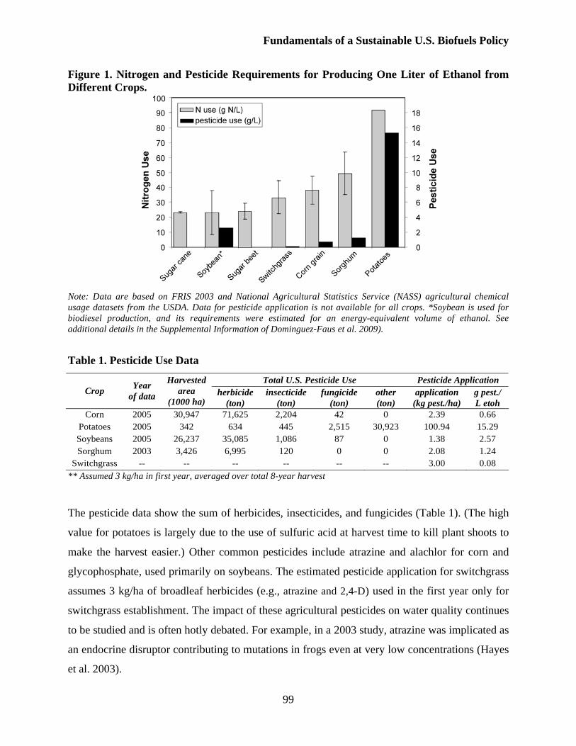
Fundamentals of a Sustainable U.S. Biofuels Policy
99
Figure 1. Nitrogen and Pesticide Requirements for Producing One Liter of Ethanol from
Different Crops.
Note: Data are based on FRIS 2003 and National Agricultural Statistics Service (NASS) agricultural chemical
usage datasets from the USDA. Data for pesticide application is not available for all crops. *Soybean is used for
biodiesel production, and its requirements were estimated for an energy-equivalent volume of ethanol. See
additional details in the Supplemental Information of Dominguez-Faus et al. 2009).
Table 1. Pesticide Use Data
Total U.S. Pesticide Use Pesticide Application
Crop Year
of data
Harvested
area
(1000 ha) herbicide
(ton)
insecticide
(ton)
fungicide
(ton)
other
(ton)
application
(kg pest./ha)
g pest./
L etoh
Corn 2005 30,947 71,625 2,204 42 0 2.39 0.66
Potatoes 2005 342 634 445 2,515 30,923 100.94 15.29
Soybeans 2005 26,237 35,085 1,086 87 0 1.38 2.57
Sorghum 2003 3,426 6,995 120 0 0 2.08 1.24
Switchgrass -- -- -- -- -- -- 3.00 0.08
** Assumed 3 kg/ha in first year, averaged over total 8-year harvest
The pesticide data show the sum of herbicides, insecticides, and fungicides (Table 1). (The high
value for potatoes is largely due to the use of sulfuric acid at harvest time to kill plant shoots to
make the harvest easier.) Other common pesticides include atrazine and alachlor for corn and
glycophosphate, used primarily on soybeans. The estimated pesticide application for switchgrass
assumes 3 kg/ha of broadleaf herbicides (e.g., atrazine and 2,4-D) used in the first year only for
switchgrass establishment. The impact of these agricultural pesticides on water quality continues
to be studied and is often hotly debated. For example, in a 2003 study, atrazine was implicated as
an endocrine disruptor contributing to mutations in frogs even at very low concentrations (Hayes
et al. 2003).
Fundamentals of a Sustainable U.S. Biofuels Policy
100
From the perspective of the total nutrient use, the increase in agriculture to meet the mandated 15
billion gallons of fuel ethanol from corn by 2015 will require an expansion of agrichemical
usage, including 2.17 million tons of additional nitrogen fertilizer, which is about 16 percent of
the N fertilizer used for all crops in the United States (National Agricultural Statistics Service
2008). The high fertilizer application rates, especially for row crops in the midwestern United
States, provide the greatest fluxes of nitrogen and phosphorus to local waterways and the
Mississippi River basin (Powers 2007), and are considered one of the primary contributors to the
growing hypoxic zone in the Gulf of Mexico, which covered over 20,000 km2 in 2007 and is
predicted to be bigger than ever in 2008. The discharge of nutrients from the Mississippi River to
the Gulf of Mexico has been measured by the USGS for decades (Figure 2). The total nitrogen
load is comprised primarily of dissolved inorganic nitrogen (DIN), with organic and particulate
nitrogen forms contributing approximately 40 percent of the total nitrogen load.
The gray lines in Figure 2 define the estimated maximum DIN export required to achieve the
federal goal for reducing the Gulf of Mexico hypoxic zone to < 5,000 km2. The upper bound (0.7
million tons-N/y) is the federal Hypoxia Task Force recommendation of a 30 percent reduction
in mean DIN load, and the lower bound (0.47 million tons-N/y) is the 55 percent reduction in
mean DIN load thought necessary to account for variability in climate and ocean dynamics.
Clearly, the current DIN loads (0.94 ± 0.26 million tons-N/y average over a 20-year period
[1984–2003]) already greatly exceed these goals. Donner and Kucharik employed a rigorous
agricultural and process-based dynamic ecosystem model to predict the impact of increased corn
production in the Midwest on nitrogen export to the Gulf of Mexico (Donner 2003; Donner and
Kucharik 2003; Donner, Kucharik, and Foley 2004; Donner and Kucharik 2008). The symbols
included in Figure 2 for the year 2015 are their estimates for the mean (± 95 percent confidence
interval) DIN exports that will result with expanded production to meet the 15 BGY corn-based
ethanol goals. The results show that the anticipated increase in corn cultivation would increase
the annual average load of DIN by 10–18 percent and increase the odds that these nitrogen loads
will exceed the target set for reducing hypoxia in the Gulf of Mexico. Thus, expanding corn-
based ethanol production would make it even more challenging to reverse the damage to this
important ecosystem and fisheries area without significant changes in agricultural management
(Goolsby et al. 2000).
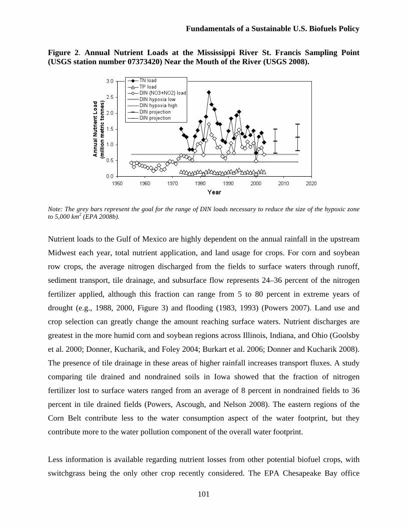
Fundamentals of a Sustainable U.S. Biofuels Policy
101
Figure 2. Annual Nutrient Loads at the Mississippi River St. Francis Sampling Point
(USGS station number 07373420) Near the Mouth of the River (USGS 2008).
Note: The grey bars represent the goal for the range of DIN loads necessary to reduce the size of the hypoxic zone
to 5,000 km2 (EPA 2008b).
Nutrient loads to the Gulf of Mexico are highly dependent on the annual rainfall in the upstream
Midwest each year, total nutrient application, and land usage for crops. For corn and soybean
row crops, the average nitrogen discharged from the fields to surface waters through runoff,
sediment transport, tile drainage, and subsurface flow represents 24–36 percent of the nitrogen
fertilizer applied, although this fraction can range from 5 to 80 percent in extreme years of
drought (e.g., 1988, 2000, Figure 3) and flooding (1983, 1993) (Powers 2007). Land use and
crop selection can greatly change the amount reaching surface waters. Nutrient discharges are
greatest in the more humid corn and soybean regions across Illinois, Indiana, and Ohio (Goolsby
et al. 2000; Donner, Kucharik, and Foley 2004; Burkart et al. 2006; Donner and Kucharik 2008).
The presence of tile drainage in these areas of higher rainfall increases transport fluxes. A study
comparing tile drained and nondrained soils in Iowa showed that the fraction of nitrogen
fertilizer lost to surface waters ranged from an average of 8 percent in nondrained fields to 36
percent in tile drained fields (Powers, Ascough, and Nelson 2008). The eastern regions of the
Corn Belt contribute less to the water consumption aspect of the water footprint, but they
contribute more to the water pollution component of the overall water footprint.
Less information is available regarding nutrient losses from other potential biofuel crops, with
switchgrass being the only other crop recently considered. The EPA Chesapeake Bay office
Fundamentals of a Sustainable U.S. Biofuels Policy
102
(Chesapeake Bay Commission 2007) modeled the potential changes in nutrient loads resulting
from increased biofuel production in the watershed, and projected a substantial reduction in
nitrogen loads to the Chesapeake Bay if cover crops are integrated into the soil (~7,800 metric
tons N/y) or if farmland is converted to switchgrass with no fertilizer (~11,500 metric tons/y). In
comparison, the Bay program partners are striving to reduce loads by 41,000 metric tons from all
sources. Thus, some of these changes will contribute substantially to that goal.
The assumption that no fertilizer would be used on the switchgrass fields in the Chesapeake Bay
region is inconsistent with other reports that recommend between zero and several hundred
kilograms of nitrogen fertilizer per hectare, with an average of 32 kg N/ha in available field trials
(see Supporting Information for Dominguez-Faus et al. 2009). These discrepancies exist because
of the lack of data associated with switchgrass cultivated as a cash crop, the uncertain
relationship between fertilizer application and increased yields, and the lack of field
measurements quantifying the fate of the fertilizer in the soil, air, and water after application.
Switchgrass uses applied N efficiently (Parrish and Fike 2005), and it appears able to obtain N
from sources that other crops cannot tap. As a result, the N removed in harvested biomass can be
greater than the amount of N applied. The long-term impacts on soil productivity are as yet
unknown. In areas with sufficient rainfall, annual sustainable switchgrass yields of 15 metric
tons/ha may be achievable by applying 50 kg N/ha (Parrish and Fike 2005). Other estimates
suggest that 90 kg N/ha would be required for switchgrass and that the fraction of the fertilizer
that was lost to surface water (30 percent) would be similar to corn (Miller, Landis et al. 2007).
With a harvest yield of 10 metric tons/ha, this would result in a loss to surface water of 12 kg
N/metric ton. The modeling study by Powers et al. assumed a much higher average fertilization
rate for switchgrass grown in Iowa (0 kg/ha in year 1 to 260 kg/ha in years 6–8), and predicted
that the average total nitrogen loads to surface water would be 7.8 kg N/ha, representing 4.2
percent of the nitrogen fertilizer applied (Powers, Ascough, and Nelson 2008).
It is better to compare among the feedstock on the basis of fuel energy generated. Table 2 shows
model predictions for a variety of crops with both conventional tillage (CT) and no-till (NT)
management practices. For the corn-soybean (CS) rotations, the no-till option reduces nutrient
(40 percent) and soil loss (75 percent) relative to conventional till and the change to harvesting
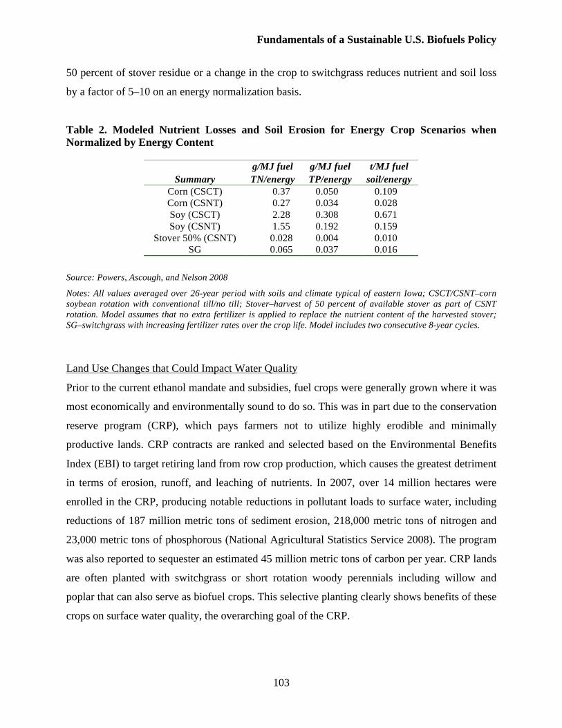
Fundamentals of a Sustainable U.S. Biofuels Policy
103
50 percent of stover residue or a change in the crop to switchgrass reduces nutrient and soil loss
by a factor of 5–10 on an energy normalization basis.
Table 2. Modeled Nutrient Losses and Soil Erosion for Energy Crop Scenarios when
Normalized by Energy Content
g/MJ fuel g/MJ fuel t/MJ fuel
Summary TN/energy TP/energy soil/energy Corn (CSCT) 0.37 0.050 0.109 Corn (CSNT) 0.27 0.034 0.028 Soy (CSCT) 2.28 0.308 0.671 Soy (CSNT) 1.55 0.192 0.159
Stover 50% (CSNT) 0.028 0.004 0.010 SG 0.065 0.037 0.016
Source: Powers, Ascough, and Nelson 2008
Notes: All values averaged over 26-year period with soils and climate typical of eastern Iowa; CSCT/CSNT–corn
soybean rotation with conventional till/no till; Stover–harvest of 50 percent of available stover as part of CSNT
rotation. Model assumes that no extra fertilizer is applied to replace the nutrient content of the harvested stover;
SG–switchgrass with increasing fertilizer rates over the crop life. Model includes two consecutive 8-year cycles.
Land Use Changes that Could Impact Water Quality
Prior to the current ethanol mandate and subsidies, fuel crops were generally grown where it was
most economically and environmentally sound to do so. This was in part due to the conservation
reserve program (CRP), which pays farmers not to utilize highly erodible and minimally
productive lands. CRP contracts are ranked and selected based on the Environmental Benefits
Index (EBI) to target retiring land from row crop production, which causes the greatest detriment
in terms of erosion, runoff, and leaching of nutrients. In 2007, over 14 million hectares were
enrolled in the CRP, producing notable reductions in pollutant loads to surface water, including
reductions of 187 million metric tons of sediment erosion, 218,000 metric tons of nitrogen and
23,000 metric tons of phosphorous (National Agricultural Statistics Service 2008). The program
was also reported to sequester an estimated 45 million metric tons of carbon per year. CRP lands
are often planted with switchgrass or short rotation woody perennials including willow and
poplar that can also serve as biofuel crops. This selective planting clearly shows benefits of these
crops on surface water quality, the overarching goal of the CRP.
Fundamentals of a Sustainable U.S. Biofuels Policy
104
Re-enrollment of lands in the CRP is dropping however, and participants are requesting early
release from CRP contracts in order to take advantage of subsidies and rapidly rising biofuels
crop prices. In 2007, Secchi and Babcock estimated that over 526 thousand hectares of Iowa
farmland would likely be pulled from the CRP and put into a corn/soybeans rotation if corn
prices hit $196 per metric ton ($5 bushel) (Secchi and Babcock 2007). In June 2008, corn rose to
nearly $314 per metric ton ($8/bushel), beyond the range modeled only one year earlier.
Although CRP contracts are established on a 10 to 15 year basis, enrollment in the program is
already decreasing. CRP enrollment dropped by more than 840,000 hectares in 2008. Due to the
erodible and less-productive nature of most land enrolled in the CRP, removing land from the
program for row crop production will likely lead to a nonlinear increase in erosion and nutrient
loading to surface waters. One proposal to avert removal of land from the CRP program is to
increase CRP payments, which totaled more than $1.6 billion in 2007 (National Agricultural
Statistics Service 2008). However, some analysts suggest that even doubling the payments would
not be sufficient to retain land in the CRP (Secchi and Babcock 2007).
3. Water and Land Requirements to Grow Energy Crops
Water and Land Demands of Biofuels from Selected Traditional Crops and Switchgrass
The water requirements of biofuel production depend on the type of feedstock used and on
geographic and climatic variables. Such factors must be considered to determine water
requirements and identify critical scenarios and mitigation strategies. Feedstock cultivation,
usually row-crop agriculture, is the most water-intensive of biofuels production stages. For
example, processing water requirements for a typical sugarcane or corn-based ethanol refinery
are around 2 to 10 liters of water per liter of ethanol produced (National Research Council 2008)
while evapotranspiration water requirements to produce enough feedstock to make one liter of
ethanol in the United States range from 500 to 5,000 liters (Figure 3). The water used in biofuel
processing and other stages in biofuel production is often withdrawn from local point sources
and can have localized impacts on water quality and quantity, despite their much lower overall
water requirements.
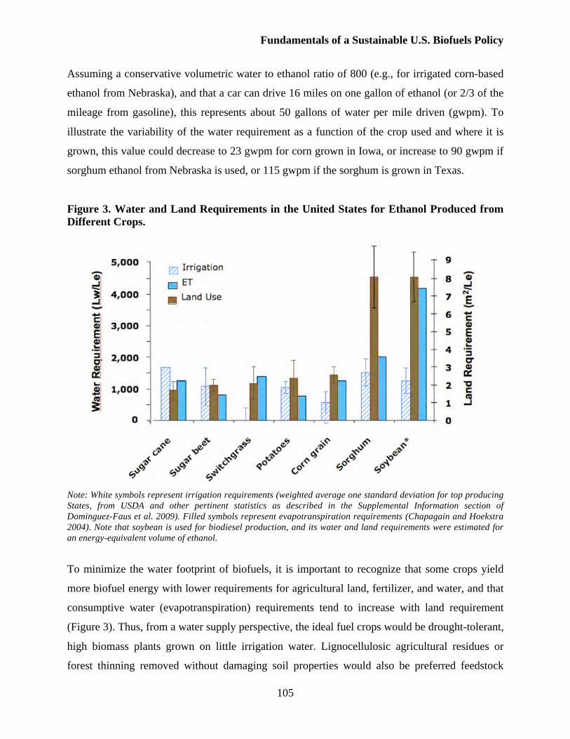
Fundamentals of a Sustainable U.S. Biofuels Policy
105
Assuming a conservative volumetric water to ethanol ratio of 800 (e.g., for irrigated corn-based
ethanol from Nebraska), and that a car can drive 16 miles on one gallon of ethanol (or 2/3 of the
mileage from gasoline), this represents about 50 gallons of water per mile driven (gwpm). To
illustrate the variability of the water requirement as a function of the crop used and where it is
grown, this value could decrease to 23 gwpm for corn grown in Iowa, or increase to 90 gwpm if
sorghum ethanol from Nebraska is used, or 115 gwpm if the sorghum is grown in Texas.
Figure 3. Water and Land Requirements in the United States for Ethanol Produced from
Different Crops.
Note: White symbols represent irrigation requirements (weighted average one standard deviation for top producing
States, from USDA and other pertinent statistics as described in the Supplemental Information section of
Dominguez-Faus et al. 2009). Filled symbols represent evapotranspiration requirements (Chapagain and Hoekstra
2004). Note that soybean is used for biodiesel production, and its water and land requirements were estimated for
an energy-equivalent volume of ethanol.
To minimize the water footprint of biofuels, it is important to recognize that some crops yield
more biofuel energy with lower requirements for agricultural land, fertilizer, and water, and that
consumptive water (evapotranspiration) requirements tend to increase with land requirement
(Figure 3). Thus, from a water supply perspective, the ideal fuel crops would be drought-tolerant,
high biomass plants grown on little irrigation water. Lignocellulosic agricultural residues or
forest thinning removed without damaging soil properties would also be preferred feedstock
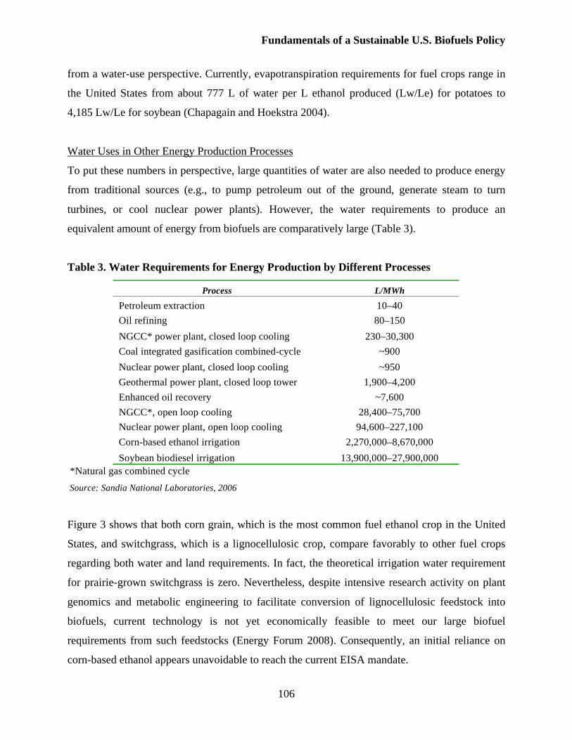
Fundamentals of a Sustainable U.S. Biofuels Policy
106
from a water-use perspective. Currently, evapotranspiration requirements for fuel crops range in
the United States from about 777 L of water per L ethanol produced (Lw/Le) for potatoes to
4,185 Lw/Le for soybean (Chapagain and Hoekstra 2004).
Water Uses in Other Energy Production Processes
To put these numbers in perspective, large quantities of water are also needed to produce energy
from traditional sources (e.g., to pump petroleum out of the ground, generate steam to turn
turbines, or cool nuclear power plants). However, the water requirements to produce an
equivalent amount of energy from biofuels are comparatively large (Table 3).
Table 3. Water Requirements for Energy Production by Different Processes
Process L/MWh
Petroleum extraction 10–40
Oil refining 80–150
NGCC* power plant, closed loop cooling 230–30,300
Coal integrated gasification combined-cycle ~900
Nuclear power plant, closed loop cooling ~950
Geothermal power plant, closed loop tower 1,900–4,200
Enhanced oil recovery ~7,600
NGCC*, open loop cooling 28,400–75,700
Nuclear power plant, open loop cooling 94,600–227,100
Corn-based ethanol irrigation 2,270,000–8,670,000
Soybean biodiesel irrigation 13,900,000–27,900,000 *Natural gas combined cycle
Source: Sandia National Laboratories, 2006
Figure 3 shows that both corn grain, which is the most common fuel ethanol crop in the United
States, and switchgrass, which is a lignocellulosic crop, compare favorably to other fuel crops
regarding both water and land requirements. In fact, the theoretical irrigation water requirement
for prairie-grown switchgrass is zero. Nevertheless, despite intensive research activity on plant
genomics and metabolic engineering to facilitate conversion of lignocellulosic feedstock into
biofuels, current technology is not yet economically feasible to meet our large biofuel
requirements from such feedstocks (Energy Forum 2008). Consequently, an initial reliance on
corn-based ethanol appears unavoidable to reach the current EISA mandate.
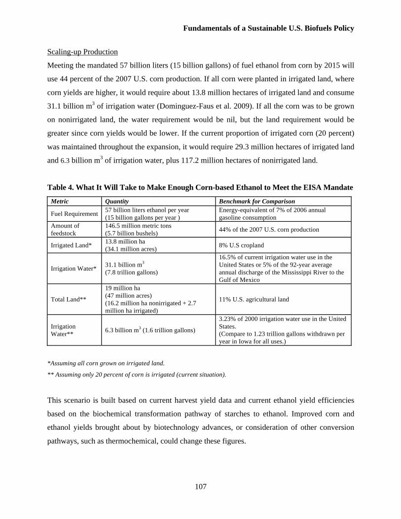
Fundamentals of a Sustainable U.S. Biofuels Policy
107
Scaling-up Production
Meeting the mandated 57 billion liters (15 billion gallons) of fuel ethanol from corn by 2015 will
use 44 percent of the 2007 U.S. corn production. If all corn were planted in irrigated land, where
corn yields are higher, it would require about 13.8 million hectares of irrigated land and consume
31.1 billion m3 of irrigation water (Dominguez-Faus et al. 2009). If all the corn was to be grown
on nonirrigated land, the water requirement would be nil, but the land requirement would be
greater since corn yields would be lower. If the current proportion of irrigated corn (20 percent)
was maintained throughout the expansion, it would require 29.3 million hectares of irrigated land
and 6.3 billion m3 of irrigation water, plus 117.2 million hectares of nonirrigated land.
Table 4. What It Will Take to Make Enough Corn-based Ethanol to Meet the EISA Mandate
Metric Quantity Benchmark for Comparison
Fuel Requirement 57 billion liters ethanol per year
(15 billion gallons per year )
Energy-equivalent of 7% of 2006 annual
gasoline consumption
Amount of
feedstock
146.5 million metric tons
(5.7 billion bushels) 44% of the 2007 U.S. corn production
Irrigated Land* 13.8 million ha
(34.1 million acres) 8% U.S cropland
Irrigation Water* 31.1 billion m3
(7.8 trillion gallons)
16.5% of current irrigation water use in the
United States or 5% of the 92-year average
annual discharge of the Mississippi River to the
Gulf of Mexico
Total Land**
19 million ha
(47 million acres)
(16.2 million ha nonirrigated + 2.7
million ha irrigated)
11% U.S. agricultural land
Irrigation
Water** 6.3 billion m3 (1.6 trillion gallons)
3.23% of 2000 irrigation water use in the United
States. (Compare to 1.23 trillion gallons withdrawn per
year in Iowa for all uses.)
*Assuming all corn grown on irrigated land.
** Assuming only 20 percent of corn is irrigated (current situation).
This scenario is built based on current harvest yield data and current ethanol yield efficiencies
based on the biochemical transformation pathway of starches to ethanol. Improved corn and
ethanol yields brought about by biotechnology advances, or consideration of other conversion
pathways, such as thermochemical, could change these figures.
Fundamentals of a Sustainable U.S. Biofuels Policy
108
Geography Matters
Expansion of corn acreage will have different consequences depending on where it occurs.
Rainfall can satisfy most of the agricultural water requirements for biofuel production in some
regions (e.g., Ohio, where less than 1 percent of corn grown is irrigated), other regions rely
primarily on irrigation (e.g., Nebraska, where 72 percent of corn grown is irrigated). This spatial
variability makes it difficult to assess the potential for increased irrigation requirements to
exacerbate competition for water resources and create local water shortages.
In already water-constrained areas, the choice of biofuel crops could lead to significant long-term
impacts. With Texas experiencing the driest spring on record in 2003 and with western states
from the Rockies to the Pacific Coast experiencing moderate to extreme droughts (Karl et al.
2008), most biofuel feedstock expansion is occurring in the Midwest where irrigated agriculture
is increasing (National Agricultural Statistics Service 2008). According to the Intergovernmental
Panel on Climate Change (IPCC) report (Kundzewicz et al. 2008) the East will get wetter and the
West will get drier. Although the East is getting wetter, precipitation is less frequent and more
intensive (Kundzewicz et al. 2008). Irrigation is necessary to provide water regularly to plants. In
Nebraska, irrigated corn area surpassed all time highs in 2007 and 2008, with over 3.64 million
hectares planted. The area is also already in all time water deficits and legal actions have been
taken by Kansas, based on allegations that Nebraska farmers used 98 billion liters more than
their allotment of the Republican River in 2004 and 2005, as ruled by the U.S. Supreme Court in
2003. Meeting the Kansas demand would mean shutting off irrigation to an estimated 485,000
hectares of Nebraska farmland. The Ogallala Aquifer is also being drawn down at record rates
(U.S. Water News Online 2009). These rates are expected to increase considerably to meet
irrigation and ethanol process water needs.
The estimates of overall water demand of scaled-up biofuel production shown in the previous
section assume expansion will happen in ideal land conditions (like those of the Corn Belt). If
expansion occurs in other not-so-suitable areas, water and land demand will be higher.
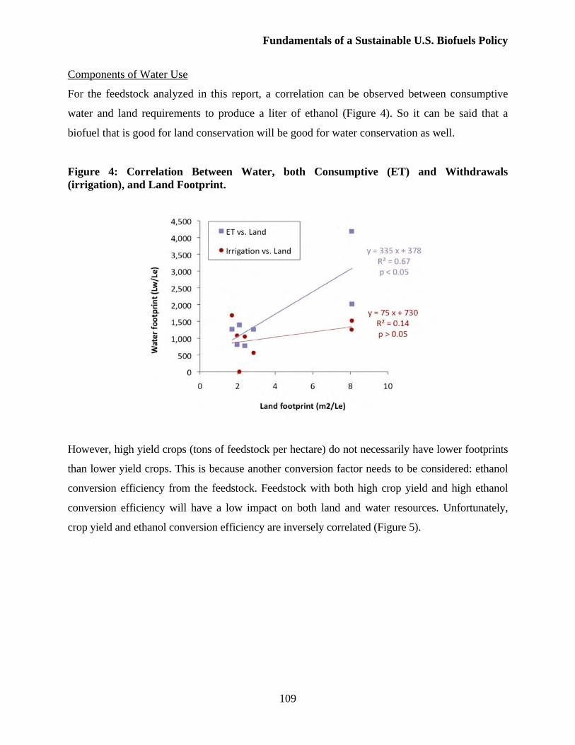
Fundamentals of a Sustainable U.S. Biofuels Policy
109
Components of Water Use
For the feedstock analyzed in this report, a correlation can be observed between consumptive
water and land requirements to produce a liter of ethanol (Figure 4). So it can be said that a
biofuel that is good for land conservation will be good for water conservation as well.
Figure 4: Correlation Between Water, both Consumptive (ET) and Withdrawals
(irrigation), and Land Footprint.
However, high yield crops (tons of feedstock per hectare) do not necessarily have lower footprints
than lower yield crops. This is because another conversion factor needs to be considered: ethanol
conversion efficiency from the feedstock. Feedstock with both high crop yield and high ethanol
conversion efficiency will have a low impact on both land and water resources. Unfortunately,
crop yield and ethanol conversion efficiency are inversely correlated (Figure 5).
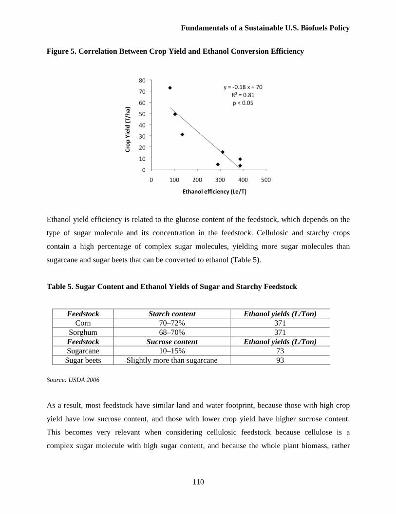
Fundamentals of a Sustainable U.S. Biofuels Policy
110
Figure 5. Correlation Between Crop Yield and Ethanol Conversion Efficiency
Ethanol yield efficiency is related to the glucose content of the feedstock, which depends on the
type of sugar molecule and its concentration in the feedstock. Cellulosic and starchy crops
contain a high percentage of complex sugar molecules, yielding more sugar molecules than
sugarcane and sugar beets that can be converted to ethanol (Table 5).
Table 5. Sugar Content and Ethanol Yields of Sugar and Starchy Feedstock
Feedstock Starch content Ethanol yields (L/Ton)
Corn 70–72% 371
Sorghum 68–70% 371
Feedstock Sucrose content Ethanol yields (L/Ton)
Sugarcane 10–15% 73
Sugar beets Slightly more than sugarcane 93
Source: USDA 2006
As a result, most feedstock have similar land and water footprint, because those with high crop
yield have low sucrose content, and those with lower crop yield have higher sucrose content.
This becomes very relevant when considering cellulosic feedstock because cellulose is a
complex sugar molecule with high sugar content, and because the whole plant biomass, rather
Fundamentals of a Sustainable U.S. Biofuels Policy
111
than the reproductive part (grain), only can be converted to ethanol, which is equivalent to
having high crop yields.
Uncertainty of Climate
Extreme hydrologic events (droughts or floods) can impact feedstock production and availability.
The 2008 floods and heavy rains in the Midwest washed away about 2 percent of the nation’s
corn crop, affecting mainly Iowa’s production (National Agricultural Statistics Service 2008).
The net effect on corn and soybean yields is yet to be determined. During 1993 flooding in the
same region, corn and soybean yields in eastern Iowa counties were reduced to 61 percent and 74
percent of the average values during the 1990s (National Agricultural Statistics Service 2006).
Extreme hydrological events are likely to persist according to the U.S. Climate Change Science
Program (Karl, Meehl et al. 2008), which infers that droughts will be more likely and severe in
the Southwest, reducing regional water supply and increasing wildfire risks. Furthermore, cold
season storms and floods will be more frequent in wet areas. On average, precipitation is likely
to be less frequent but more intense, while heat waves are likely to increase and, consequently,
more irrigation water would be necessary. Thus, in addition to geographical variability, temporal
variability in water availability and in crop requirements confound our ability to determine the
potential for biofuel irrigation to exacerbate competition for water resources and contribute to
water shortages.
Water Use Projections for Other Sectors
Energy and agriculture already rank as the top two sectors in U.S. water withdrawals, accounting
respectively for 48 percent and 34 percent of the total (Hutson et al. 2004). Regardless of climate
change, the competition for water between these two sectors will intensify in the near future. The
Energy Information Administration (EIA) predicts that thermoelectric generation from coal,
natural gas, nuclear and other fuels will increase by 22 percent between 2005 and 2030 (Donner
and Kucharik 2008), for example. Combined with a biofuel-induced increase in agricultural
water use of 16.5 percent by 2015 (Table 4), the potential to create water shortages and conflicts
cannot be dismissed.
Fundamentals of a Sustainable U.S. Biofuels Policy
112
4. Greenhouse Gases and Air Quality Effects Associated with Biofuels Production and Use.
Air quality is regulated by the Clean Air Act (CAA), which was last amended in 1990 although
some minor changes have occurred since then. The CAA requires the U.S. EPA to set National
Ambient Air Quality Standards (NAAQs) for six common air pollutants: carbon monoxide (CO),
nitrogen oxides (NOx), sulfur dioxide (SO2), lead (Pb), ozone (O3), and particulate matter (PM).
These six pollutants are known as “criteria pollutants” since the permissible levels of pollution
are based on health and/or environmental criteria. Other gaseous emissions of environmental
concern are those called greenhouse gas (GHG) emissions since it is believed that there has been
an unprecedented accumulation of these gases in the atmosphere since the industrialization, and
that they are causing anthropogenically-driven global warming. Carbon dioxide (CO2), methane
(CH4), and nitrous oxide (N2O) are among the most prominent GHGs affected by biofuel
production.
Air Pollutants of Concern
Not only are GHGs important when considering air quality implications of biofuels, but there are
other air pollutants of concern.
Criteria Pollutants
Criteria pollutants are six common pollutants regulated by EPA based on human and
environmental health guidelines. Such regulated pollutants are:
Carbon Monoxide (CO)
CO reduces oxygen delivery to human organs and tissues and is associated with heart
problems; it induces vision problems and in extremely high levels can cause death. CO
emissions are mainly produced during incomplete combustion of fuels. Biofuel blends,
ethanol-gasoline or diesel-biodiesel result in decreasing rates of CO emissions, because the
oxygen content of the biofuels allows for better fuel combustion. Values ranging from 10 to
30 percent smaller can be found (Pikunas, Pukalskas, and Grabys 2003; Yuksel and Yuksel
2004), with an ethanol-gasoline blend. For diesel-biodiesel, such values can reach 50 percent,
depending on the amount of biodiesel in the mixture (Lapuerta, Armas, and Rodriguez-
Fundamentals of a Sustainable U.S. Biofuels Policy
113
Fernandez 2008). Although tailpipe CO emissions are smaller when using E-10 or E-85, life
cycle emissions from E-85 are substantially higher than E-0 (Winebrake, He, and Wang
2000). Compared with conventional diesel, life cycle emissions for biodiesel can be
considered smaller (Hill et al. 2006).
Nitrogen Oxides (NOx)
The two most important nitrogen oxide pollutants are nitric oxide (NO) and nitrogen dioxide
(NO2). These pollutants are emitted when fossil fuels are burned. In 2003, transportation
accounted for 57 percent of emissions whereas stationary fuel combustion sources were
responsible for 37 percent. Of the anthropogenic emissions of NOx, 95 percent are in the
form of NO, which has no known adverse health effects at concentrations found in the
atmosphere. However NO readily oxidizes to NO2, which can irritate lungs, causes bronchitis
and pneumonia, as well as lower resistance to respiratory problems. NO2 can also react with
OH in the atmosphere to form nitric acid (HNO3), contributing to the acid rain problem.
NOx are also key precursor to another criteria pollutant: ground-level ozone (O3). Results on
literature regarding biofuel impacts on NOx are diverse. While some suggest tailpipe
emission reduction ranging from 30 to 45 percent, when using E-85 (Jacobson 2007). Others
suggest no changes (Graham, Belisle, and Baas 2008) or increases ranging from 6 percent
(Cooney 2007) to 50 percent (Kim and Dale 2004). Biodiesel blends are responsible for
linear increases in NOx emissions as the content of biodiesel in the mixture increases with
reductions of about 12 percent for pure biodiesel (Lapuerta et al. 2008). Life cycle analysis
(LCA) for NOx emissions, compared with base fuels, can be considered higher for both
ethanol (6–7 percent) and diesel (12 percent).
There is a trade-off between reduction in emissions of carbon monoxide and nitrogen oxides.
At higher combustion temperatures, however, there is a reduction in emissions of CO while
emissions of NOx increase.
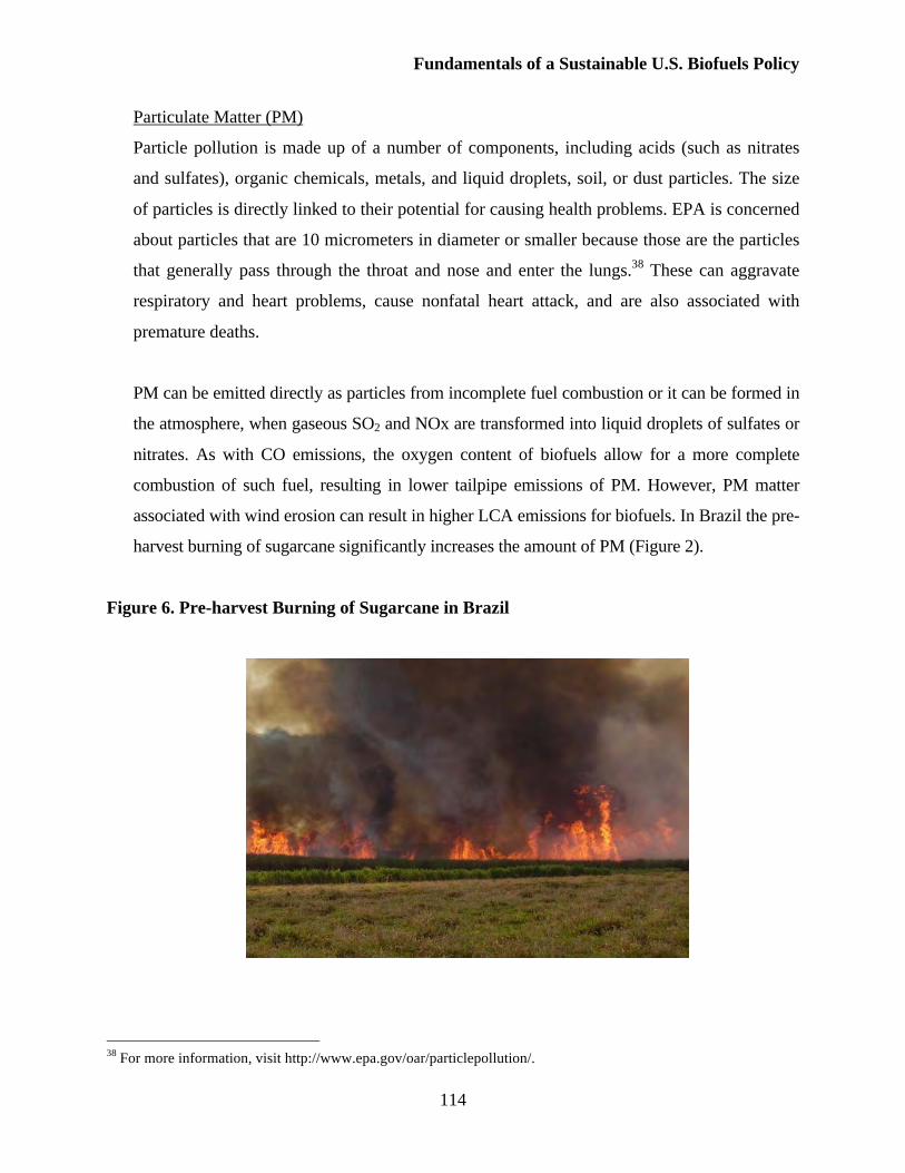
Fundamentals of a Sustainable U.S. Biofuels Policy
114
Particulate Matter (PM)
Particle pollution is made up of a number of components, including acids (such as nitrates
and sulfates), organic chemicals, metals, and liquid droplets, soil, or dust particles. The size
of particles is directly linked to their potential for causing health problems. EPA is concerned
about particles that are 10 micrometers in diameter or smaller because those are the particles
that generally pass through the throat and nose and enter the lungs.38 These can aggravate
respiratory and heart problems, cause nonfatal heart attack, and are also associated with
premature deaths.
PM can be emitted directly as particles from incomplete fuel combustion or it can be formed in
the atmosphere, when gaseous SO2 and NOx are transformed into liquid droplets of sulfates or
nitrates. As with CO emissions, the oxygen content of biofuels allow for a more complete
combustion of such fuel, resulting in lower tailpipe emissions of PM. However, PM matter
associated with wind erosion can result in higher LCA emissions for biofuels. In Brazil the pre-
harvest burning of sugarcane significantly increases the amount of PM (Figure 2).
Figure 6. Pre-harvest Burning of Sugarcane in Brazil
38 For more information, visit http://www.epa.gov/oar/particlepollution/.
Fundamentals of a Sustainable U.S. Biofuels Policy
115
Sulfur Oxides (SOx)
SO2 causes a wide variety of health and environmental impacts because of the way it reacts
with other substances in the air. Particularly sensitive groups include people with asthma who
are active outdoors, children, the elderly, and people with heart or lung disease
(Environmental Protection Agency 2009).
SOx are not a concern in terms of tailpipe emissions from motor vehicles. About 80 percent
of the anthropogenic SOx emissions are the result of fossil fuel combustion in stationary
sources, mostly coal-fired power plants. The only significant noncombustion sources of
sulfur emissions are associated with petroleum refining, copper smelting, and cement
manufacture. SOx emissions are associated with biofuels by the use of energy (electricity)
either for irrigation or distillery energy supply. It is also associated with natural gas used in
ethanol milling plants. Literature does not devote much attention for SOx LCA emissions.
Overall results are still not clear, although the literature considers increases of SOx in LCA
balances.
Ozone (O3) – Tropospheric
Ozone is related to respiratory problems such as coughing, throat irritation, bronchitis,
emphysema, and asthma. Tropospheric ozone is commonly formed in the presence of
sunlight with NOx and volatile organic compounds (VOC). Since both increase with the use
of biofuels, the tendency is for ozone to increase as well. An interesting study of possible
consequences of E-85 use concluded that it “may increase ozone-related mortality,
hospitalization, and asthma by about 9% in Los Angeles and 4% in the United States as a
whole relative to 100% gasoline” (Jacobson 2007).
Volatile Organic Compounds (VOC)
VOC causes damage to the central nervous system and can cause cancer in humans and
animals. Fatigue, nausea, and headaches are also symptoms associated with VOC exposure.
This class of compounds consists of volatile compounds that enter the atmosphere when
solvents, fuels, and other organics evaporate. The transportation sector is responsible for
almost half of anthropogenic VOC emissions. This review focuses on five VOC compounds:
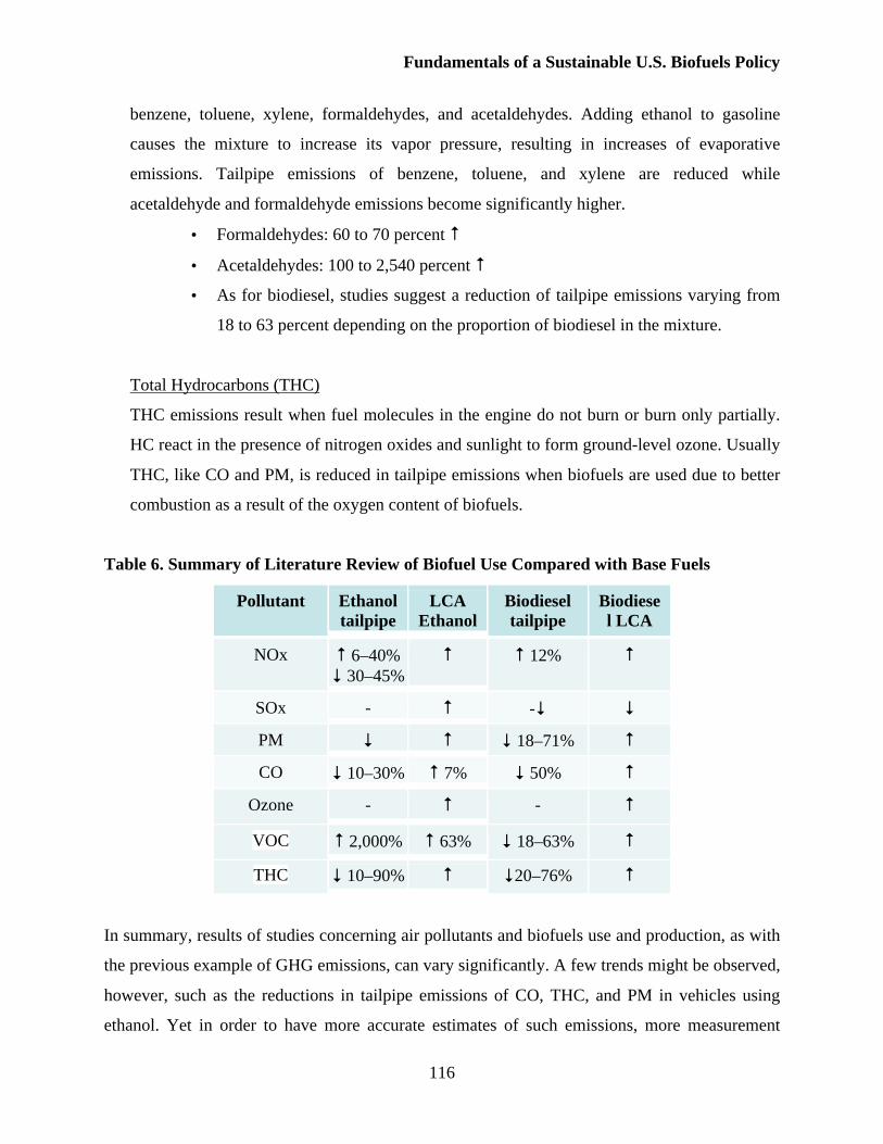
Fundamentals of a Sustainable U.S. Biofuels Policy
116
benzene, toluene, xylene, formaldehydes, and acetaldehydes. Adding ethanol to gasoline
causes the mixture to increase its vapor pressure, resulting in increases of evaporative
emissions. Tailpipe emissions of benzene, toluene, and xylene are reduced while
acetaldehyde and formaldehyde emissions become significantly higher.
• Formaldehydes: 60 to 70 percent
• Acetaldehydes: 100 to 2,540 percent
• As for biodiesel, studies suggest a reduction of tailpipe emissions varying from
18 to 63 percent depending on the proportion of biodiesel in the mixture.
Total Hydrocarbons (THC)
THC emissions result when fuel molecules in the engine do not burn or burn only partially.
HC react in the presence of nitrogen oxides and sunlight to form ground-level ozone. Usually
THC, like CO and PM, is reduced in tailpipe emissions when biofuels are used due to better
combustion as a result of the oxygen content of biofuels.
Table 6. Summary of Literature Review of Biofuel Use Compared with Base Fuels
Pollutant Ethanol
tailpipe
LCA
Ethanol
Biodiesel
tailpipe
Biodiese
l LCA
NOx 6–40%
30–45%
12%
SOx - -
PM 18–71%
CO 10–30% 7% 50%
Ozone - -
VOC 2,000% 63% 18–63%
THC 10–90% 20–76%
In summary, results of studies concerning air pollutants and biofuels use and production, as with
the previous example of GHG emissions, can vary significantly. A few trends might be observed,
however, such as the reductions in tailpipe emissions of CO, THC, and PM in vehicles using
ethanol. Yet in order to have more accurate estimates of such emissions, more measurement
Fundamentals of a Sustainable U.S. Biofuels Policy
117
experiments should be performed. That is true not only for tailpipe emissions, but as in the case
of PM, for agriculture field emissions as well.
Research Needs
Geographical Distribution of Criteria Pollutants
Impacts on air pollution resulting from the use of biofuels tend to vary locally due to a series of
factors. For instance, NOx emissions are associated with vehicle tailpipes while PM can be also
important in agricultural areas due to wind erosion. SOx emissions, on the other hand, are
associated with electricity consumed during different phases of biofuel production. Besides such
aspects, local atmospheric conditions have an important role on the concentration of certain
pollutants. Local atmospheric conditions not only affect air movement patterns, but they also
impact local assimilation capacity and the complex interactions among pollutants in the
atmosphere.
To maximize the benefits of biofuels and, in some ways, dilute their environmental impact,
careful consideration should be given to the location of agricultural fields and biofuel plants, as
well as the cities that primarily consume the fuels.
Professor Daniel Cohan’s research group at Rice University has begun to address these issues by
conducting air quality modeling for alternate scenarios of biodiesel deployment in the Houston
region. Devoting the nation’s entire soybean crop to biodiesel production would displace only 6
percent of total diesel use (Hill et al. 2006), and other feedstock face limited availability as well
(Hanna, Isom, and Campbell 2005). Targeting biodiesel toward applications with maximal
environmental benefit is thus crucial to optimizing its potential impact, especially if biodiesel is
to be deployed in a pure form.
Despite the dozens of studies comparing the emissions from biodiesel and diesel on a tailpipe or
life cycle basis, no published studies have yet examined how deployment and use of biodiesel
could be targeted to optimize its air quality and health impacts. For example, for a given amount
of biodiesel, what would be the relative impacts of deploying it broadly in low percentage blends
Fundamentals of a Sustainable U.S. Biofuels Policy
118
versus targeting its use in higher blends to specific parts of the diesel fleet? Densely populated
areas may stand to gain the most from biodiesel’s propensity to reduce PM, CO, hydrocarbons,
and air toxics, all of which have limited atmospheric lifetimes and directly harm human health
(Brunekreef and Holgate 2002).
Human and Environmental Health Assessment
Additionally, to better assess GHG and pollutant emissions, it would be recommended that at
some point this data could be used to evaluate the impacts on human health of such emissions.
This can be accomplished by the use of the risk-assessment approach. Such an approach can also
be useful to assess environmental impacts, some of which are discussed in other sections of this
document.
Land Use Change – CO2, CH4, N2O Emissions
If biofuel production continues to receive incentives, it is very likely that land area devoted to
biofuel crops will increase. This report noted earlier that this could lead to increased carbon
emissions. Existing projections for future land use devoted to biofuel crops can be useful to
estimate the net increase or decrease of CO2, CH4, and N2O emissions by comparing this land
use with current land uses. N2O emissions could also be used to calculate how land use changes
ultimately affect stratospheric O3 emissions.
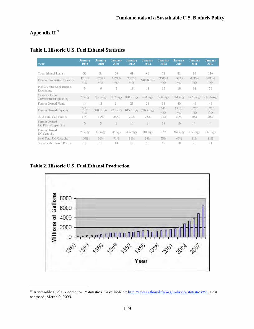
Fundamentals of a Sustainable U.S. Biofuels Policy
119
Appendix II39
Table 1. Historic U.S. Fuel Ethanol Statistics
Table 2. Historic U.S. Fuel Ethanol Production
39 Renewable Fuels Association. “Statistics.” Available at: http://www.ethanolrfa.org/industry/statistics/#A. Last
accessed: March 9, 2009.
Year
January
1999
January
2000
January
2001
January
2002
January
2003
January
2004
January
2005
January
2006
January
2007
Total Ethanol Plants 50 54 56 61 68 72 81 95 110
Ethanol Production Capacity 1701.7 mgy
1748.7 mgy
1921.9 mgy
2347.3 mgy
2706.8 mgy 3100.8 mgy
3643.7 mgy
4336.4 mgy
5493.4 mgy
Plants Under Construction/ Expanding
5 6 5 13 11 15 16 31 76
Capacity Under Construction/Expanding
77 mgy 91.5 mgy 64.7 mgy 390.7 mgy 483 mgy 598 mgy 754 mgy 1778 mgy 5635.5 mgy
Farmer Owned Plants 14 18 21 25 28 33 40 46 46
Farmer Owned Capacity 293.3 mgy
340.3 mgy 473 mgy 645.6 mgy 796.6 mgy 1041.1 mgy
1388.6 mgy
1677.1 mgy
1677.1 Mgy
% of Total Cap Farmer 17% 19% 25% 28% 29% 34% 38% 39% 39%
Farmer Owned UC Plants/Expanding
5 3 3 10 8 12 10 4 4
Farmer Owned UC Capacity
77 mgy 60 mgy 60 mgy 335 mgy 318 mgy 447 450 mgy 187 mgy 187 mgy
% of Total UC Capacity 100% 66% 71% 86% 66% 75% 60% 11% 11%
States with Ethanol Plants 17 17 18 19 20 19 18 20 21
Fundamentals of a Sustainable U.S. Biofuels Policy
120
Reference List
Akinci, B., P.G. Gassebaum, J.V. Fitch, and R.W. Thompson. “The Role of Bio-Fuels in Satisfying
US Transportation Fuel Demands.” Energy Policy 36, no. 9 (2008): 3485–3491.
Alvarez, P.J.J., and T.M. Vogel. “Degradation of BTEX and their aerobic metabolites by
indigenous microorganisms under nitrate reducing conditions.” Water Science and
Technology 31, no. 1 (1995): 15–28.
Alvarez, P.J.J., and C.S. Hunts. “The Effect of Ethanol on BTEX Biodegradation and Natural
Attenuation, Potential Ground and Surface Water Impacts.” In “Potential Ground and
Surface Water Impacts,” edited by G. Cannon and D. Rice, Chapter 3. 1999. http://www-
erd.llnl.gov/ethanol/etohdoc/vol4/chap03.pdf.
American Council of Governmental Industrial Hygienists. Documentation of the Threshold Limit
Values and Biological Exposure Indices, 6th ed. Cincinnati, Ohio, 1991.
Anderson, R.T., J.N. Rooney-Varga, C.V. Gaw, and D.R. Lovley. “Anaerobic Benzene
Oxidation in the Fe(III) Reduction zone of Petroleum-contaminated Aquifers.”
Environmental Science and Technology 32, no. 9 (1998): 1222–1229.
Araujo, D.B., B. Butler, and C. Mayfield. “Effects of Gasoline and Ethanol Mixtures on Aquifer
Microorganisms.” Poster presented at the 48th annual meeting of the Canadian Society of
Microbiologists, Guelph, Ontario, Canada, 1998.
Armstrong, S.R. “Ethanol–Its Use in Gasoline: Expected Impacts and Comments of Expert
Reviewers.” Cambridge, Massachusetts: Cambridge Environmental, Inc., 2000.
Association of Oil Pipe Lines and American Petroleum Institute. “Ethanol and Pipeline
Transportation Policy Paper.” February 2007.
http://www.aopl.org/pdf/AOPL_API_Ethanol_Transportation_Final144839.pdf (accessed
March 2, 2009).
Barker, J. F., C. E. Hubbard, L. A. Lemon, and K. A. Vooro. “The Influence of Methanol in
Gasoline Fuels on the Formation of Dissolved Plumes, and the Fate and Natural
Remediation of Methanol and BTEX Dissolved in Groundwater.” In Hydrocarbon
Contaminated Soils and Groundwater, edited by E. J. Calabrese and P. T. Kostecki, 103–
113. New York: Lewis Publishers, 1992.
Brunekreef, B. and S.T. Holgate. “Air Pollution and Health.” Lancet 360 (2002): 1233–1242.
Fundamentals of a Sustainable U.S. Biofuels Policy
121
Brusseau, M., A. Wood, and P. Rao. “Influence of Organic Solvents on the Sorption Kinetics of
Hydrophobic Organic Chemicals.” Environmental Science and Technology 25, no. 5
(1991): 903–910.
Burkart, M., D. James, M. Liebman, and E. van Ouwerkerk. “Integrating Principles of Nitrogen
Dynamics in a Method to Estimate Leachable Nitrogen Under Agricultural Systems.”
Water Science and Technology 53, no. 2 (2006): 289–301.
Bush, George W. State of the Union address, January 23, 2007. Text available at
http://frwebgate.access.gpo.gov/cgi-
bin/getdoc.cgi?dbname=2007_record&docid=cr23ja07-120.
Cápiro, N.L, B.P. Stafford, W.G. Rixey, P.B. Bedient, and P.J.J. Alvarez. “Fuel-grade Ethanol
Transport and Impacts to Groundwater in a Pilot-scale Aquifer Tank.” Water Research
41, no. 3 (2007): 656–664.
Cápiro, N.L, M.L. Da Silva, B.P. Stafford, W.G. Rixey, and P.J.J. Alvarez. “Microbial
Community Response to a Release of Neat Ethanol Onto Residual Hydrocarbons in a
Pilot-scale Aquifer Tank.” Environmental Microbiology 10, no. 9 (2008): 2236–2244.
Chapagain, A.K., and A.Y. Hoekstra. Water Footprints of Nations, Volume 1. UNESCO-IHE,
2004. http://www.waterfootprint.org/Reports/Report16Vol1.pdf.
Chesapeake Bay Commission. “Biofuels and the Bay: Getting It Right to Benefit Farms, Forests
and the Chesapeake.” September 2007.
http://www.chesbay.state.va.us/Publications/BiofuelsAndTheBay1.pdf.
Chiu Y.W., B. Walseth, and S. Suh. “Water Embodied in Bioethanol in the U.S.” Environmental
Science and Technology 43, no. 8 (2009): 2688–2692.
Clayton, G., and F. Clayton. Patty’s Industrial Hygiene and Toxicology, fourth edition. New
York: John Wiley & Sons, 1994.
Colares, Juscelino F. “A Brief History of Brazilian Biofuels Legislation.” Syracuse Journal of
Law & Commerce 35, no. 2 (2008).
Congressional Budget Office. “The Impact of Ethanol Use on Food Prices and Greenhouse-Gas
Emissions.” April 2009. http://www.cbo.gov/ftpdocs/100xx/doc10057/04-08-
Ethanol.pdf.
Cooney, C.M. “Higher Ozone Levels from Renewable Fuels.” Environmental Science and
Technology, June 15, 2007.
Fundamentals of a Sustainable U.S. Biofuels Policy
122
Corseuil, H., C. Hunt, R. dos Santos Ferreira, and P.J.J. Alvarez. “The Influence of the Gasoline
Oxygenate Ethanol on Aerobic and Anaerobic BTX Biodegradation.” Water Research
32, no. 7 (1998): 2065–2072.
Crutzen, P.J., A.R. Mosier, K.A. Smith, and W. Winiwarter. “N2O Release from Agro-biofuel
Production Negates Global Warming Reduction by Replacing Fossil Fuels.” Atmospheric
Chemistry and Physics Discussions 7, no. 4 (2007): 11,191–11,205.
Dakhel, N., G. Pasteris, D. Werner, and P. Hohener. “Small-volume Releases of Gasoline in the
Vadose Zone: Impact of the Additives MTBE and Ethanol on Ground Water Quality.”
Environmental Science and Technology 10 (2003): 2127–2133.
Da Silva, M.L.B., and P.J.J. Alvarez. “Effects of Ethanol Versus MTBE on BTEX Migration and
Natural Attenuation in Aquifer Columns.” Journal of Environmental Engineering 128,
no. 9 (2002): 862–867.
Davis, S., and D.J. Weiss. “Progressive Relief from High Fuel Prices.” Center for American
Progress. May 1, 2008. http://www.americanprogress.org/issues/2008/05/reliefbate.html
(accessed June 22, 2009).
De La Torre Ugarte, D.G., B.C. English, R. Jamey Menard, and M. Walsh. “Conditions that
Influence the Economic Viability of Ethanol from Corn Stover in the Midwest of the
USA.” International Sugar Journal 108 (2006): 152–156.
Deeb, R.A., J.O. Sharp, A. Stocking, S. McDonald, K.A. West, M. Laugier, P.J.J. Alvarez, M.C.
Kavanaugh, and L. Alvarez-Cohen. “Impact of Ethanol on Benzene Plume Lengths:
Microbial and Modeling Studies.” Journal of Environmental Engineering—ASCE 128,
no. 9 (2002): 868–875.
Dias de Oliveira, Marcelo E. “Ethanol Fuel.” Presentation at “Biomass to Chemicals and Fuels:
Science, Technology and Public Policy” conference, Houston, Texas, September 25–26, 2006.
Dodds, W.K., W.W. Bouska, J.L. Eitzmann, T.J. Pilger, K.L. Pitts, A.J. Riley, J.T. Schloesser,
and D.J. Thornbrugh. “Eutrophication of U.S. Freshwaters: Analysis of Potential
Economic Damages.” Environmental Science and Technology 43, no. 1 (2009): 12–19.
Dominguez-Faus, R., S.E. Powers, J.G. Burken, and P.J.J. Alvarez. “The Water Footprint of
Biofuels: A Drink or Drive Issue?” Environmental Science & Technology 43, no. 9
(2009): 3005–3010.
Fundamentals of a Sustainable U.S. Biofuels Policy
123
Donner S.D. “The Impact of Cropland Cover on River Nutrient Levels in The Mississippi River
Basin.” Global Ecology and Biogeography 12, no. 4 (2003): 341–355.
Donner S.D., and C.J. Kucharik. “Corn-based Ethanol Production Compromises Goal of
Reducing Nitrogen Export by the Mississippi River.” Proceedings of the National
Academy of Sciences of the United States of America 105, no. 11 (2008): 4513–4518.
Donner, S.D., C.J. Kucharik, and J.A. Foley. “Impact of Changing Land Use Practices on Nitrate
Export by the Mississippi River.” Global Biogeochemical Cycles 18, no. 1 (2004): 1–21.
Doering, O.C., F. Diaz-Hermelo, C. Howard, R. Heimlich, F. Hitzhusen, R. Kazmierczak, J. Lee,
et al. Evaluation of Economic Costs and Benefits of Methods for Reducing Nutrient Loads
to the Gulf of Mexico (Report of Task Group 6 to White House Committee on
Environment and Natural Resources, Hypoxia Work Group.) Silver Spring, Maryland:
U.S. Department of Commerce, National Oceanic and Atmospheric Administration,
Coastal Ocean Program, April 1999.
DTN Ethanol Center. “Renewable Fuels Standards Policy Updates (by state).” January 10, 2008.
http://www.dtnethanolcenter.com/index.cfm?show=10&mid=16&pid=1.
Duetz, W.A., S. Marques, C. de Jong, J.L. Ramos, and J.G. Van Andel. “Inducibility of the TOL
Catabolic Pathway in Pseudomonas putida (pWWO) Growing on Succinate in
Continuous Culture: Evidence of Carbon Catabolite Repression.” Journal of Bacteriology
176 (1994): 2354–2361.
Dutka B.J., and K.K. Kwan. “Comparison of Three Microbial Toxicity Screening Tests with the
Microtox Test.” Bulletin of Environmental Contamination and Toxicology 27 (1981): 753–757.
Egli T. “The Ecological and Physiological Significance of the Growth of Heterotrophic
Microorganisms with Mixtures of Substrates.” Advances in Microbial Ecology 14 (1995):
305–386.
Energy Forum, James A. Baker III Institute for Public Policy. “U.S. Biofuels Policy: Progress
and Challenges.” Workshop, Houston, Texas, August 20, 2008.
http://www.rice.edu/energy/events/past/20Aug08_Biofuelworkshop.html.
ExxonMobil. “Algae Biofuel.”
http://www.exxonmobil.com/Corporate/energy_climate_con_vehicle_algae.aspx
(accessed December 10, 2009).
Fundamentals of a Sustainable U.S. Biofuels Policy
124
Fargione J., J. Hill, D. Tilman, S. Polasky, and P. Hawthorne. “Land Clearing and the Biofuel
Carbon Debt.” Science 319 (2008): 1235–1238.
Farrell, A., R.J. Pleving, B.T. Turner, A.D. Jones, M. O’Hare, and D.M.Kammen. “Ethanol Can
Contribute to Energy and Environmental Goals.” Science 311 (2006): 506–508.
Fereres, E., and M. Auxiliadora Soriano. “Deficit Irrigation for Reducing Agricultural Water
Use.” Journal of Experimental Botany 58, no. 2 (2007): 147–159.
Food and Agricultural Organization. “Indicators Definitions.”
http://www.fao.org/economic/ess/other-statistics/socio-economic-agricultural-and-
environmental-indicators/database-on-macro-economic-indicators/indicators-
definitions/en/.
Food and Agricultural Organization: Statistics (FAOSTAT). “Production: Crops.”
http://faostat.fao.org/site/567/default.aspx#ancor.
Frisman, Paul. “Ethanol as an Alternative Fuel.” Connecticut Office of Legislative Research.
Report 2006-R-0524, 2006.
Gollehon, N., and W. Quinby. “Irrigation Resources and Water Costs.” Agricultural Resources
and Environmental Indicators, 2006 Edition. Economic Research Service, U.S.
Department of Agriculture.
Gomez D.E., and P.J.J. Alvarez. “Modeling the Natural Attenuation of Benzene in Groundwater
Impacted by Ethanol-blended Fuels: Effect of Ethanol Content on the Lifespan and
Maximum Length of Benzene Plumes.” Water Resources Research 45, no. 3 (2009):
article W03409.
Gomez, D.E., P.C. de Blanc, W. Rixey, P.B. Bedient, and P.J.J Alvarez. “Modeling Benzene
Plume Elongation Mechanisms Exerted by Ethanol Using RT3D with a General Substrate
Interaction Module.” Water Resouces Research 44, no. 5 (2008).
Goolsby D.A., W.A. Battaglin, B.T. Aulenbach, and R.P. Hooper. “Nitrogen Flux and Sources in the
Mississippi River Basin.” Science of the Total Environment 248, no. 2–3 (2000): 75–86.
Goolsby, D.A., W.A. Battaglin, G.B. Lawrence, R.S. Artz, B.T. Aulenbach, R.P. Hooper, D.R.
Kenney, and G.J. Stensland. Flux and Sources of Nutrients in the Mississippi-Atchafalaya
River Basin (Report of Task Group 3 to White House Committee on Environment and
Natural Resources, Hypoxia Work Group). Silver Spring, Maryland: U.S. Department of
Fundamentals of a Sustainable U.S. Biofuels Policy
125
Commerce, National Oceanic and Atmospheric Administration, Coastal Ocean Program,
May 1999.
Graham L., S.L. Belisle, and C.L Baas. “Emissions from Light-duty Gasoline Vehicles
Operating on Low-blend Ethanol Gasoline and E85.” Atmospheric Environment 42, no.
19 (2008): 4498–4516.
Hanna, M.A., L. Isom, and J. Campbell. “Biodiesel: Current Perspectives and Future.” Journal of
Scientific and Industrial Research 64, no. 11: (2005): 854–857.
Harold, F. “Antimicrobial Agents and Membrane Function.” Advances in Microbial Physiology
4 (1970): 45–104.
Hayes, T.K,. Haston, M. Tsui, A. Hoang, C. Haeffele, and A.Vonk. “Atrazine-Induced
Hermaphroditism at 0.1 ppb in American Leopard Frogs (Rana pipiens): Laboratory and
Field Evidence.” Environmental Health Perspectives 111, no. 4 (2003): 568–575.
Heermann, S. E., and S. E. Powers. “Modeling the Partitioning of BTEX in Water-reformulated
Gasoline Systems Containing Ethanol.” Journal of Contaminant Hydrology 34 (1998):
315–341.
Heermann, S. E., and S. E. Powers. “The Dissolution of BTEX Compounds from Oxygenated
Gasoline.” American Chemical Society Division of Environmental Chemistry preprints of
extended abstracts, 212th ACS, 36, no. 1 (1996): 221–224.
Hill J., E. Nelson, D. Tilman, S. Polasky, and D. Tiffany. “Environmental, Economic, and
Energetic Costs and Benefits of Biodiesel and Ethanol Biofuels.” Proceedings of the
National Academy of Sciences of the United States of America 103, no. 30 (2006):
11206–11210.
Holford, N. “Clinical Pharmacokinetics of Ethanol.” Clinical Pharmacokinetics 13, no. 5 (1987):
273–292.
Howard, P.H., R.S. Boethling, W.F Jarvis, W.M. Meylan, and E.M. Michalenko. Handbook of
Environmental Degradation Rates. Chelsea, Michigan: Lewis Publishers, 1991.
Hunt, C.S. “Effect of Alternative Substrates on the Biodegradation of Monoaromatic
Hydrocarbons.” Ph.D. diss., University of Iowa, 1999.
Hunt, C.S., P.J.J. Alvarez, R. dos Santos Ferreira, and H. Corseuil. “Effect of Ethanol on Aerobic
BTEX Degradation.” In In situ and Onsite Bioremediation, edited by B.C. Alleman and
A. L. Lesson. Columbus, Ohio: Battelle Press, 1997, 49–54.
Fundamentals of a Sustainable U.S. Biofuels Policy
126
Hutson, S.S., N.L. Barber, J.F. Kenny, K.S. Linsey, D.S. Lumia, and M.A. Maupin. “Estimated Use
of Water in the United States 2000.” U.S. Geological Survey: Reston, Virginia, 2004.
Ingram, L., and T. Buttke. “Effects of Alcohols on Micro-organisms.” Advances in Microbial
Physiology 25 (1984): 253–303.
Jacobson, M.Z. “Effects of Ethanol (E85) Versus Gasoline Vehicles on Cancer and Mortality in
the United States.” Environmental Science Technology 41, no. 11 (2007): 4150–4157.
Karl, T.R., G.A. Meehl, C.D. Miller, S.J. Hassol, A.M. Waple, and W.L. Murray, eds. “Weather and
Climate Extremes in a Changing Climate.” Final Report, Synthesis and Assessment Product
3.3. Department of Commerce, NOAA’s National Climatic Data Center, Washington, D.C.,
June 2008. http://www.climatescience.gov/Library/sap/sap3-3/final-report/.
Keeney, D., and M. Muller. “Water Use by Ethanol Plants.” Institute for Agriculture and Trade
Policy. October 2006. http://www.agobservatory.org/library.cfm?RefID=89449.
Kim, S., and B.E. Dale. “Global Potential Bioethanol Production from Wasted Crops and Crop
Residues.” Biomass and Bioenergy 26 (2004): 361–375.
Kinder Morgan. Presentation at the “U.S. Biofuels Policy: Progress and Challenges” Workshop,
Energy Forum, James A. Baker III Institute for Public Policy, Houston, Texas, August
20, 2008.
Kundzewicz, Z.W., L.J. Mata, N.W. Arnell, P. Döll, B. Jimenez, K. Miller, T. Oki, Z. Sen, and I.
Shiklomanov. “The Implications of Projected Climate Change for Freshwater Resources
and Their Management.” Hydrological Sciences Journal 53, no. 1 (2008): 3–10.
Lapuerta, M., O. Armas, and J. Rodríguez-Fernández. “Effect of Biodiesel Fuels on Diesel Engine
Emissions.” Progress in Energy and Combustion Science 34, no. 2 (2008): 198–223.
Lasko, D., C. Schwerdel, J. Bailey, and U. Sauer. “Acetate-specific Stress Response in Acetate-
resistance Bacteria: An Analysis of Protein Patterns.” Biotechnology Progress 13 (1997):
519–523.
Lamm, F.R., and T.P. Trooien. “Subsurface Drip Irrigation for Corn Production: A Review of 10
Years of Research in Kansas.” Irrigation Science 22, no. 3–4 (2003): 195–200.
Livingston, M.L., and A. Garrido. ”Entering the Policy Debate: An Economic Evaluation of
Groundwater Policy in Flux.” Water Resources Research 40, no. 12 (2004): 1–11.
Fundamentals of a Sustainable U.S. Biofuels Policy
127
Lovanh, N., and P.J.J. Alvarez. “Effect of Ethanol, Acetate, and Phenol on Toluene Degradation
Activity and Tod-lux Expression in Pseudomonas Putida TOD102: Evaluation of the
Metabolic Flux Dilution Model.” Biotechnology Bioengineering 86, no. 7 (2004): 801–808.
Lovanh, N., C.S. Hun, and P.J.J. Alvarez. “Effect of Ethanol on BTEX Biodegradation Kinetics:
Aerobic Continuous Culture Experiments.” Water Resources 36 (2002): 3739–3746.
Madigan, J. T., J. M. Martinko, and J. Parker. Brock Biology of Microorganisms, 11th ed. Upper
Saddle River, NJ: Prentice-Hall, 2005.
Madson, F.W., and Monceaux, D.A. “Fuel Ethanol Production.” Cincinnati: KATZEN
International, Inc., 2003.
http://www.bioethanol.ru/images/bioethanol/Fuel%20ethanol%20production%20-
%20Katzen.pdf.
Maryland Department of the Environment. “Methyl Tertiary Butyl Ether (MTBE) and Clean
Gasoline Alternatives.” January 2006.
http://www.mde.state.md.us/assets/document/air/MTBEReport_Jan2006.pdf.
Marrone, P.A., K.R. Liberty, and D.J. Turton. “Review of Emerging Optimization Opportunities
for Corn-to-Ethanol Production.” Ethanol Producer Magazine, October-December 2008.
http://www.ethanolproducer.com/articles/EmergingOptimizationOpportunities/.
McCarty, P. L. “Anaerobic Waste Treatment Fundamentals, Part Three—Toxic Materials and
Their Control.” Public Works 95 (1964): 91–94.
McCarty, P. L. “Energetics and Bacterial Growth.” Fifth Rudolf Research Conference, Rutgers,
The State University, New Brunswick, New Jersey, 1969.
McGuire, V.L. “Ground Water Depletion in the High Plains Aquifer.” Fact Sheet 2007–3029.
U.S. Geological Survey: Reston, Virginia, 2007.
McNab, W., S. E. Heermann, and B. Dooher. “Screening Model Evaluation of the Effects of
Ethanol on Benzene Plume Lengths.” California Environmental Council Report UCRL-
AR-135949, Ch. 4, 1999.
Mesa-Lago, C. “The Cuban Economy in 2004–2005.” Paper presented at the annual meeting of
the Association for the Study of the Cuban Economy, Miami, Florida, August 4–6, 2005.
http://lanic.utexas.edu/project/asce/pdfs/volume15/.
Miller, S.A., A.E. Landis, and T.L. Theis. “Environmental Trade-offs of Biobased Production.”
Environmental Science and Technology 41 (15), (2007): 5176–5182.
Fundamentals of a Sustainable U.S. Biofuels Policy
128
Minnesota Pollution Control Agency. “Ethanol-Blended Fuel Releases Guidance Document 1-
06.” September 2008. http://www.pca.state.mn.us/publications/c-prp1-06.pdf.
Molson, J.W., J.F. Barker, and E.O. Frind. “Modeling the Impact of Ethanol on the Persistence
of Benzene in Gasoline-Contaminated Groundwater.” Water Resources Research 38, no.
1 (2002): 41–412.
Morris, David. “The Carbohydrate Economy, Biofuels and the Net Energy Debate.” Institute for
Local Self-Reliance. August 2005.
http://www.newrules.org/sites/newrules.org/files/images/netenergyresponse.pdf.
Monod, J. “The Growth of Bacterial Cultures.” Annual Review of Microbiology 3 (1949): 371–394.
Mummey, D.L., J.L. Smith, and G. Bluhm. “Assessment of Alternative Soil Management
Practices on N2O Emissions from U.S. Agriculture.” Agriculture, Ecosystems and
Environment 70, no. 1 (1998): 79–87.
National Research Council. Water Implications of Biofuels Production in the United States.
Washington, D.C.: The National Academies Press, 2008.
Nebraska Department of Environmental Quality. “Reported Ethanol Spills to NDEQ.” 2005.
Lincoln, Nebraska. Personal communication with Dave Chambers.
Perez-Lopez, Jorge F. “The Cuban Economy in 2002–2003.” Paper presented at the annual
meeting of the Association for the Study of the Cuban Economy, Coral Gables, Florida,
August 7–9, 2003. http://lanic.utexas.edu/project/asce/pdfs/volume13/.
Pikunas, A., S. Pukalskas, and J. Grabys. “Influence of Composition of Gasoline-ethanol Blends
on Parameters of Internal Combustion Engines.” Journal of Kones Internal Combustion
Engines 10, 3-4 (2003): 205–211.
Pohorecky, L. and J. Brick. Pharmacology and Therapeutics 36, no. 2–3 (1988): 335–427.
Pollitt, B. “The Rise and Fall of the Cuban Sugar Economy.” Journal of Latin American Studies
36 (2004): 319–348.
Parrish, D.J., and J.H. Fike. “The Biology and Agronomy of Switchgrass for Biofuels.” Critical
Reviews in Plant Sciences 24, no. 5–6 (2005): 423–459.
Petrolia, D.R., and P.H. Gowda. “Missing the Boat: Midwest Farm Drainage and Gulf of Mexico
Hypoxia.” Review of Agricultural Economics 28, no. 2 (2006): 240–253.
Fundamentals of a Sustainable U.S. Biofuels Policy
129
Pimentel, D., and T.W.Patzek. “Ethanol Production Using Corn, Switchgrass, and Wood:
Biodiesel Production Using Soybean and Sunflower.” Natural Resources Research 14,
no. 1 (2005): 65–76.
Powers, S.E. “Nutrient Loads to Surface Water from Row Crop Production.” International
Journal of Lifecycle Assessment 12, no. 6 (2007): 399–407.
Powers, S.E., L.A. Ascough, and R.G. Nelson. “Soil and Water Quality Implications Associated
With Corn Stover Removal and Herbaceous Energy Crop Production in Iowa. In
Proceedings of the 2008 Annual International Meeting of the American Society of
Agricultural and Biological Engineers. Providence, Rhode Island, 2008.
Powers, S.E., C.S. Hunt, S.E. Heermann, H.X. Corseuil, D. Rice, and P.J.J Alvarez. “The
Transport and Fate of Ethanol and BTEX in Groundwater Contaminated by Gasohol.”
Critical Reviews in Environmental Sciences and Technology 31, no. 1 (2001): 79–123.
Powers, S.E., and C.J. McDowell. “Infiltration and Distribution of Ethanol and Ethanol-blended
Gasoline in the Vadose Zone.” Subsurface Fate and Transport of Gasoline Containing
Ethanol, Chapter 2, UCRL-AR-145380, (2001).
Pretty, J.N., C.F. Mason, D.B. Nedwell, R.E. Hine, S. Leaf, and R. Dils. “Environmental Costs
of Freshwater Eutrophication in England and Wales.” Environmental Science and
Technology 37 (2003): 201–208.
Rabalais, N.N., R.E. Turner, W.J. Wiseman Jr. “Hypoxia in the Gulf of Mexico, a.k.a. the Dead
Zone.” Annual Review of Ecology and Systematics 33, no. 1 (2002): 235–263.
Rabl, Ari, and Josheph V. Spadaro. “Environmental Impacts and Costs of Energy.” Annals of the
New York Academy of Sciences 1076 (2006): 516–26.
Rao, P.S.C., A.G. Hornsby, D.P. Kilcrease, P. Nkedi-Kizza. “Sorption and Transport of
Hydrophobic Organic Chemicals in Aqueous and Mixed Solvent Systems: Model
Development and Preliminary Evaluation. Journal of Environmental Quality 14 (1985):
376–383.
Renewable Fuels Association. “Resources–VEETC.” http://www.ethanolrfa.org/resource/veetc/
(accessed December 11, 2008).
Renewable Fuels Association. “Statistics.” http://www.ethanolrfa.org/industry/statistics/
(accessed October 23, 2009).
Fundamentals of a Sustainable U.S. Biofuels Policy
130
Ribaudo, M.O., R. Heimlich, and M. Peters. “Nitrogen Sources and Gulf Hypoxia: Potential for
Environmental Credit Trading.” Ecological Economics 52 (2005): 159–168.
Rubin, O.D., M. Carriquiry, and D.J. Hayes. “Implied Objectives of U.S. Biofuel Subsidies.”
Center for Agricultural and Rural Development, Working Paper 08-WP 459 (2008): 1–
31. http://www.card.iastate.edu/publications/synopsis.aspx?id=1065.
Ruiz-Aguilar, G.M.L., J. M. Fernandez-Sanchez, S. R. Kane, D. Kim, and P.J.J. Alvarez. “Effect
of Ethanol and Methyl-tert-butyl Ether on Monoaromatic Hydrocarbon Biodegradation:
Response Variability for Different Aquifer Materials Under Various Electron-accepting
Conditions.” Environmental Toxicology and Chemistry 21, no. 12 (2002): 2631–2639.
Ruiz-Aguilar, G.M.L., K. O’Reilly, and P.J.J. Alvarez. “A Comparison of Benzene and Toluene
Plume Lengths for Sites Contaminated with Regular vs. Ethanol-amended Gasoline.”
Ground Water Monitoring and Remediation 23, no. 1 (2003): 48–53.
Sandia National Laboratories. “Energy Demands on Water Resources—Report to Congress on
the Interdependency of Energy and Water.” December 2006.
http://www.sandia.gov/energy-water/congress_report.htm.
Schlesinger, W.H. Biogeochemistry: An Analysis of Global Change. San Diego: Academic Press, 1997.
Searchinger T., R. Heimlich, R.A. Houghton, F. Dong, A. Elobeid, J. Fabiosa, S. Tokgoz, D.
Hayes, and T.H. Yu. “Use of U.S. Croplands for Biofuels Increases Greenhouse Gases
through Emissions from Land-use Change.” Science 319 (2008): 1238–1240.
Secchi S., and B. Babcock. “Impact of High Crop Prices on Environmental Quality: A Case of
Iowa and the Conservation Reserve Program.” Center for Agricultural and Rural
Development, Iowa State University. May 2007.
Secchi, S., P.W. Gassman, M. Jha, L. Kurkalova, H.H. Feng, T. Campbell, and C.L. Kling. “The
Cost of Cleaner Water: Assessing Agricultural Pollution Reduction at the Watershed
Scale.” Journal of Soil and Water Conservation. 62 (2007): 10–21.
Sekely, A. Personal interview with J. Coan, June 2009.
Shapouri, H., J.A. Duffield, and M. Wang. “The Energy Balance of Corn Ethanol: An Update.”
U.S. Department of Agriculture, Office of the Chief Economist, Office of Energy Policy
and New Uses. Agricultural Economic Report No. 814, July 2002.
Speece, R.E. “Anaerobic Biotechnology for Industrial Wastewater Treatment.” Environmental
Science and Technology 17, no. 9 (1983): 416A–426A.
Fundamentals of a Sustainable U.S. Biofuels Policy
131
Squillace, P.J., J.S. Zogorski, W.G. Wilber, and C.V. Price. Preliminary Assessment of the
Occurrence and Possible Sources of MTBE in Groundwater in the United States, 1993–
1994.” Environmental Science and Technology 30 (1996): 1721–1730.
Styles, G., and R. Acosta. “Hitting the Blend Wall.” Herold Alternative Energy Insights, March 5, 2009.
Solomon, B.D., J.R. Barnes, and K.E. Halvorsen. “Grain and Cellulosic Ethanol: History,
Economics, and Energy Policy.” Biomass and Bioenergy 31 (2007): 416–425.
Suflita, J.M., and M.R. Mormile. “Anaerobic Biodegradation of Known and Potential Gasoline
Oxygenates in the Terrestrial Subsurface.” Environmental Science and Technology 27
(1993): 976–978.
Taylor, S.W., and P.R. Jaffe. “Biofilm Growth and the Related Changes in the Physical
Properties of a Porous Medium – 1. Experimental Investigation.” Water Research 26, no.
9 (1990): 2153–2159.
Ulrich, G. “The Fate and Transport of Ethanol-Blended Gasoline in the Environment: A
Literature Review and Transport Modeling.” Submitted by the Governors’ Ethanol
Coalition, Lincoln, Nebraska, October 1999.
http://www-erd.llnl.gov/FuelsoftheFuture/pdf_files/fatereport.pdf.
United States (Federal) Alternative Fuel Dealer.
http://www.afdc.energy.gov/afdc/progs/view_ind_mtx.cgi?user/AFS/US/0.
Urbanchuk, John M. “Contribution of the Ethanol Industry to the Economy of the United States.”
Prepared for the Renewable Fuels Association, February 20, 2008.
http://www.ethanolrfa.org/objects/documents/1537/2007_ethanol_economic_contribution.pdf.
U.S. Department of Agriculture. Economic Research Service. 2008 Farm Bill Side-By-Side –
Title XV: Trade and Tax Provisions.
http://www.ers.usda.gov/farmbill/2008/titles/titleXVTradeTax.htm
U.S. Department of Agriculture. The Economic Feasibility of Ethanol Production from Sugar in
the United States. July 2006.
http://www.usda.gov/oce/reports/energy/EthanolSugarFeasibilityReport3.pdf.
U.S. Department of Agriculture. National Agricultural Statistics Service.
http://www.nass.usda.gov (accessed April 16, 2009).
Fundamentals of a Sustainable U.S. Biofuels Policy
132
U.S. Department of Agriculture. National Agricultural Statistics Service. “2007 Corn Crop a
Record Breaker, USDA Reports,” news release, January 11, 2008.
http://www.nass.usda.gov/Newsroom/2008/01_11_2008.asp.
U.S Department of Energy. E85: An Alternative Fuel.
http://www.afdc.energy.gov/afdc/ethanol/e85.html (accessed May 20, 2009).
U.S. Department of Energy. Energy Information Administration. Annual Energy Outlook 2007.
U.S. Department of Energy. Energy Information Administration. Biofuels in the U.S.
Transportation Sector. 2007b.
U.S. Department of Energy. Energy Information Administration. Federal Financial
Interventions and Subsidies in Energy Markets 2007. April 9, 2008.
http://www.eia.doe.gov/oiaf/servicerpt/subsidy2/index.html.
U.S. Department of Energy. Office of Energy Efficiency & Renewable Energy. “DOE to Invest
$786.5 Million in Recovery Act Funds in Biofuels,” news release, May 6, 2009.
http://www1.eere.energy.gov/biomass/news_detail.html?news_id=12490 (accessed June
1, 2009).
U.S. Department of Transportation 2007. Pipeline and Hazardous Materials Safety
Administration. “General Pipeline FAQs.” Last Updated August 29, 2007.
U.S. Environmental Protection Agency. 2008a. Cleaning Up Underground Storage Tank System
Releases. http://www.epa.gov/swerust1/cat/index.htm.
U.S. Environmental Protection Agency. Hypoxia in the North Gulf of Mexico. EPA-SAB-08-003.
Washington, D.C., 2008b.
U.S. Environmental Protection Agency. Sulfur Dioxide: Health and Environmental Impacts of
SO2. http://www.epa.gov/air/urbanair/so2/hlth1.html (accessed May 13, 2009).
U.S. General Accounting Office. “Tax Incentives for Petroleum and Ethanol Fuels.”
GAO/RCED-00-301R. September 2000. http://www.gao.gov/archive/2000/rc00301r.pdf.
U.S. Geological Survey. Hypoxia in the Gulf of Mexico Studies. Reston, Virginia, 2008.
http://toxics.usgs.gov/hypoxia.
U.S. Geological Survey. Pesticides in the Nation’s Streams and Ground Water, 1992–2001.
http://pubs.usgs.gov/circ/2005/1291/.
U.S. Water News Online, “Ogallala Aquifer has shrunk 9 percent, new report says,” April 2009.
http://www.uswaternews.com/archives/arcsupply/9ogalaqui4.html.
Fundamentals of a Sustainable U.S. Biofuels Policy
133
Vandevivere, P., and P. Baveye. “Relationship Between Transport of Bacteria and Their
Clogging Efficiency in Sand Columns.” Applied Environmental Microbiology 58, no. 8
(1992): 2523–2530.
Ward, F.A., and M. Pulido-Velazquez. “Water Conservation in Irrigation Can Increase Water
Use.” Proceedings of the National Academy of Sciences of the United States of America
105, no. 47 (2008): 18,215-18,220.
Weiner, J. M., and D. R. Lovley. “Anaerobic Benzene Degradation in Petroleum-contaminated
Aquifer Sediments After Inoculation with a Benzene-oxidizing Enrichment.” Applied
Environmental Microbiology 64, no. 2 (1998): 775–778.
Wessler, Justus. “Opportunities (‘costs’) matter: A comment on Pimentel and Patzek ‘Ethanol
production using corn, switchgrass, and wood; biodiesel production using soybean and
sunflower,’” Energy Policy 35, no. 2: 1414–1416.
Winebrake J.J., D.Q. He, and M.Q. Wang. “Fuel-cycle Emissions for Conventional and
Alternatives Fuel Vehicles – An Assessment of Air Toxics.” August 2000. Argonne
National Laboratory. Report # ANL/ESD-44.
Yüksel, F., and B. Yüksel, B. “The Use of Ethanol-gasoline Blend as a Fuel in an SI
Engine.” Renewable Energy 29, no. 7 (2004):1181–1191.
Zhang, Y., I.A. Khan, X.-H. Chen, and R.F. Spalding. “Transport and Degradation of Ethanol in
Groundwater.” Journal of Contaminant Hydrology 82, no. 3–4 (2006): 183–194.