Fundamental Experiments with the Tucker Decomposition in theMatlab Tensor Toolbox

Sergio Garcia Tapia1, Rebecca Hsu2, Alyssa Hu3, Darren Stevens II4

1Department of Mathematics, University at Buffalo, SUNY2Department of Mathematics, University of Maryland, College Park3Department of Mathematics and Department of Computer Science,

University of Maryland, College Park4Department of Computer Science and Electrical Engineering, UMBC

Advisor: Matthias K. Gobbert, gobbert@umbc.edu,Department of Mathematics and Statistics, UMBC

Abstract

This report explores how data structures known as tensors can be used to perform multi-dimensional data analysis. If a matrix can be thought of as a two-dimensional array, then atensor can be thought of as a multi-dimensional array (with more than two dimensions). Tensordecompositions are algorithms and tools that can allow the user to directly perform analysison this type of data. After explaining the basics of tensors, we work with two different three-dimensional data sets and decompose the tensors in order to provide analysis and interpretationsof various aspects of the data. We show in detail how to use commands from the Matlab TensorToolbox to set up the problems and compute the Tucker decomposition.

Key words. Tensors, Tucker tensors, Tucker decomposition, Matlab Tensor Toolbox, Princi-pal component analysis.

1 Introduction

Many application problems in data analysis inherently contain multi-dimensional data. Potentialexamples can include behavioral studies across different situations, facial recognition algorithms,and signals processing and analysis. Matrices are oftentimes used to organize the variables reorderedafter having found an appropriate way to express the data in the two-dimensional array. On theother hand, one can also directly perform analysis on the data by using multi-dimensional arraysthat preserve the inherent structure of such multi-dimensional data represented by tensors.

The basics of how to use and operate with tensors are similar to operations with regular two-dimensional matrices. With third-order (three-dimensional) tensors, it is clearer to visualize themas slices of matrices overlayed on top of each other. Multiplying tensors requires an extra step;one must unfold the tensor into a matrix before proceeding with traditional matrix multiplicationand then refold the result back into a higher order tensor. For multi-dimensional data, one wouldnormally perform dimension reduction techniques to organize the data into a matrix. Then, amethod such as principal component analysis (PCA) would be applied on the matrix in order toprovide analysis of the data. However, we can apply what is known as a tensor decomposition toall of the multi-dimensional data at once. One specific tensor decomposition for N -dimensionaltensors is called the Tucker decomposition [5]; specifically for 3-dimensional data, Kiers et al. [4]also refer to it as 3-mode-PCA (3MPCA). This decomposition factors the original data into a coretensor that is typically smaller, as well as three factor matrices that measure the level of interaction

1

between the data [5]. Section 2 introduces some basic facts and properties of tensors and explainsthe Tucker decomposition more in-depth.

The Matlab Tensor Toolbox1 has many functions available for creating and operating withtensors, some of which we will discuss in Section 3. The Tensor Toolbox can be used to performbasic operations on both dense and sparse tensors, such as set up and multiply tensors with othertensors and with other vectors or matrices. There are in fact functions for working with tensorsthat have specific properties, as well as relevant decompositions, such as Tucker or Kruskal tensors.Section 3 discusses the features of the Matlab Tensor Toolbox in more detail.

In order to provide an illustrative example, Kiers [4] provides a fictitious set of data as abehavioral study for six different individuals measuring five behavioral responses in four differentscenarios. This data is naturally multi-dimensional and can be expressed as a 6×5×4 tensor. Kiersapplies the 3MPCA decomposition to this data to generate the component matrices and desiredcore tensor. Labels were given to each of the components after seeing the column groupings inorder to provide a clear interpretation of the data. Kiers demonstrates mathematically how to usethe results of the decomposition in order to retrieve the original data. This is shown in detail inSection 4.

Section 5 introduces data from a Dutch psychological experiment with a 326×5×2 tensor. Weapply the Tucker decomposition also to this data set and then use additional steps to analyze theresult. Kiers used the component matrices’ columns to group data and generated labels for thosecolumns. For the Dutch data set, we take the dot product of the original data with the columns ofone of the component matrices to better summarize the data. We note how we can input differentcore tensor sizes and if that affects resulting component matrices and interpretation.

Section 6 summarizes the conclusions from our calculations using the Matlab Tensor Toolboxand provides an outlook to larger problems.

2 Tensor Analysis

2.1 Tensor Basics

We now formally introduce tensors. Material presented here is based on the Kolda and Baderpaper [5]. Recall that a matrix U ∈ RI×J can be thought of as a 2-dimensional array, whereI, J are positive integers. A tensor X ∈ RI1×···×IN is a generalization of a matrix; that is, it isan N -dimensional array. As such, many properties and operations of matrices are retained inhigher dimensions with some concepts being more intricate. Tensors are denoted by Euler scriptcharacters as first done above in the usage of X. An element in a tensor is denoted by xi1,...,iN , wherein = 1, . . . , In (that is, the subscripts range from 1 to their corresponding uppercase equivalent).An N -dimensional tensor is also referred to sometimes as a tensor of order N , or a tensor with Nmodes. Addition is done element-wise as one would expect, and the Frobenius norm of a tensor isthe same as that of a matrix, satisfying

||X|| =

√√√√ I1∑i1=1

· · ·IN∑

iN=1

x2i1,...,iN for X ∈ RI1×···×IN .

1Version 2.6, http://www.sandia.gov/~tgkolda/TensorToolbox/index-2.6.html

2

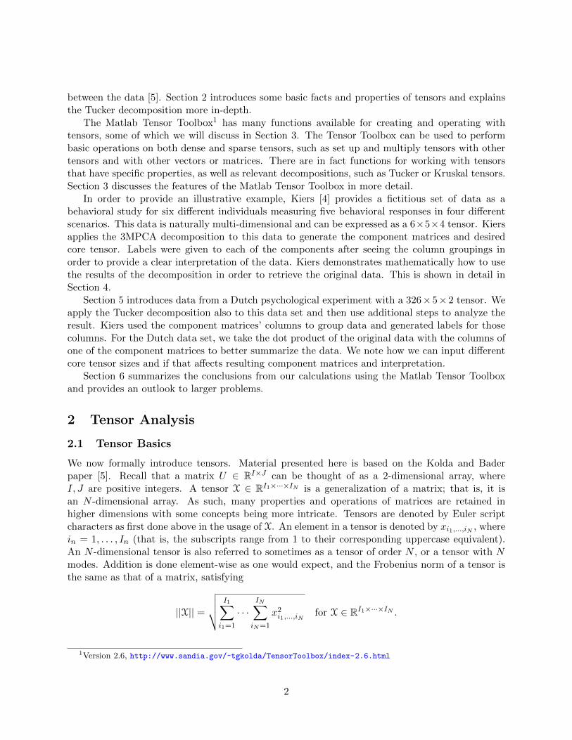
Figure 2.1: A tensor of order 3.

For N -way tensor X, fibers and slices are defined by fixing N−1 and N−2 indices, respectively.The fibers then are 1-dimensional tensors or arrays (vectors), and the slices are 2-dimensionaltensors or arrays (matrix) obtained from X with some orientation that depends on what indiceshave been fixed. For illustrative purposes, we limit our discussion to 3-way tensors and provideFigure 2.1 as a way to visualize them. For a tensor X ∈ RI×J×K of 3 dimensions, on the one hand,a fiber is obtained by fixing two of the indices. The possible choices then are vectors X(:, j, k),X(i, :, k), and X(i, j, :), for i = 1, . . . , I, j = 1, . . . , J , and k = 1, . . . ,K; these correspond tocolumns, rows, and tube fibers, respectively. In Figure 2.2, we see that fibers of a 3-way tensor arepillars with some orientation. On the other hand, a slice of a tensor X is obtained by fixing oneof the indices and the choices would be matrices X(i, :, :), X(:, j, :), and X(:, :, k) that correspondto horizontal, lateral, and frontal slices, respectively. In Figure 2.3, we see that the the slices of a3-way tensor are represented as planes with certain orientations.

Introducing fibers also allows us to introduce the idea of unfolding tensors. Visually, the mode-nunfolding or matricization of a 3-way tensor G ∈ RP×Q×R, where n = 1, 2, or 3, means to take themode-n fibers, to rotate them into column orientation, and then line them up sequentially. Theresult is that we express a tensor G as a matrix G(n) with dimensions that depend on n = 1, 2, 3, aswell as P,Q,R. The benefit of this is that it allows us to consider mode-n matrix multiplication.The mode-n product between a tensor and matrix is defined if certain dimensions match as is thecase for matrices. If G ∈ RP×Q×R is a tensor of 3 modes, and if G(3) ∈ RR×PQ is its mode-3

unfolding, then the mode-3 product with a matrix C ∈ RK×R is expressed as

Y = G×3 C ⇐⇒ Y(3) = CG(3).

where Y ∈ RP×Q×K , and Y(3) ∈ RK×PQ is its mode-3 unfolding. An example of this is explored indetail in Section 4.

2.2 Principal Component Analysis

Many methods for dealing with multi-dimensional data by using matrices have been developed.Among them is principal component analysis (PCA), a technique that seeks to find an appropriaterepresentation for data that has been collected and organized in a matrix. Generally, data isarranged in a matrix U such that each column constitutes a different type of measurement performed

3

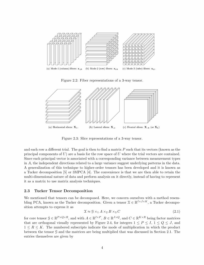
Figure 2.2: Fiber representations of a 3-way tensor.

Figure 2.3: Slice representations of a 3-way tensor.

and each row a different trial. The goal is then to find a matrix P such that its vectors (known as theprincipal components of U) are a basis for the row space of U where the trial vectors are contained.Since each principal vector is associated with a corresponding variance between measurement typesin A, the independent directions related to a large variance suggest underlying patterns in the data.A generalization of this technique to higher-order tensors has been developed and it is known asa Tucker decomposition [5] or 3MPCA [4]. The convenience is that we are then able to retain themulti-dimensional nature of data and perform analysis on it directly, instead of having to representit as a matrix to use matrix analysis techniques.

2.3 Tucker Tensor Decomposition

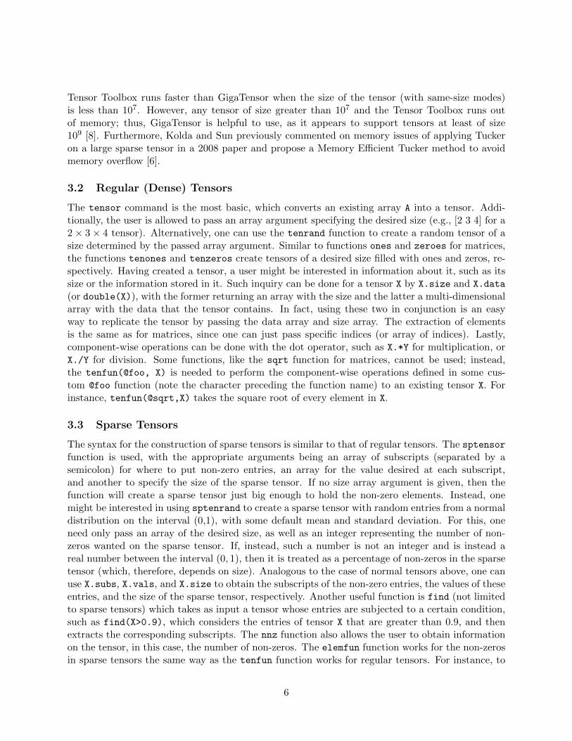
We mentioned that tensors can be decomposed. Here, we concern ourselves with a method resem-bling PCA, known as the Tucker decomposition. Given a tensor X ∈ RI×J×K , a Tucker decompo-sition attempts to express it as

X ≈ G×1 A×2 B ×3 C (2.1)

for core tensor G ∈ RP×Q×R, and with A ∈ RI×P , B ∈ RJ×Q, and C ∈ RK×R being factor matricesthat are orthogonal visually represented by Figure 2.4, for integers 1 ≤ P ≤ I, 1 ≤ Q ≤ J , and1 ≤ R ≤ K. The numbered subscripts indicate the mode of multiplication in which the productbetween the tensor G and the matrices are being multiplied that was discussed in Section 2.1. Theentries themselves are given by

4

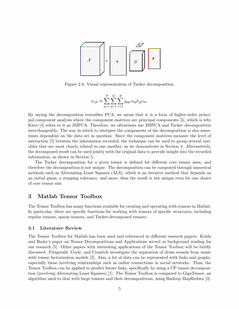
Figure 2.4: Visual representation of Tucker decomposition.

xijk ≈P∑

p=1

Q∑q=1

R∑r=1

gpqraipbjqckr.

By saying the decomposition resembles PCA, we mean that it is a form of higher-order princi-pal component analysis where the component matrices are principal components [5], which is whyKiers [4] refers to it as 3MPCA. Therefore, we oftentimes use 3MPCA and Tucker decompositioninterchangeably. The way in which to interpret the components of the decomposition is also some-times dependent on the data set in question. Since the component matrices measure the level ofinteraction [5] between the information recorded, the technique can be used to group several vari-ables that are most closely related to one another, as we demonstrate in Section 4. Alternatively,the decomposed result can be used jointly with the original data to provide insight into the recordedinformation, as shown in Section 5.

The Tucker decomposition for a given tensor is defined for different core tensor sizes, andtherefore the decomposition is not unique. The decomposition can be computed through numericalmethods such as Alternating Least Squares (ALS), which is an iterative method that depends onan initial guess, a stopping tolerance, and more, thus the result is not unique even for one choiceof core tensor size.

3 Matlab Tensor Toolbox

The Tensor Toolbox has many functions available for creating and operating with tensors in Matlab.In particular, there are specific functions for working with tensors of specific structures, includingregular tensors, sparse tensors, and Tucker-decomposed tensors.

3.1 Literature Review

The Tensor Toolbox for Matlab has been used and referenced in different research papers. Koldaand Bader’s paper on Tensor Decompositions and Applications served as background reading forour research [5]. Other papers with interesting applications of the Tensor Toolbox will be brieflydiscussed. Fitzgerald, Coyle, and Cranitch investigate the separation of drum sounds from musicwith tensor factorization models [2]. Also, a lot of data can be represented with links and graphs,especially those involving relationships such as online connections in social networks. Thus, theTensor Toolbox can be applied to predict future links, specifically by using a CP tensor decomposi-tion (involving Alternating Least Squares) [1]. The Tensor Toolbox is compared to GigaTensor, analgorithm used to deal with large tensors and their decompositions, using Hadoop MapReduce [3].

5

Tensor Toolbox runs faster than GigaTensor when the size of the tensor (with same-size modes)is less than 107. However, any tensor of size greater than 107 and the Tensor Toolbox runs outof memory; thus, GigaTensor is helpful to use, as it appears to support tensors at least of size109 [8]. Furthermore, Kolda and Sun previously commented on memory issues of applying Tuckeron a large sparse tensor in a 2008 paper and propose a Memory Efficient Tucker method to avoidmemory overflow [6].

3.2 Regular (Dense) Tensors

The tensor command is the most basic, which converts an existing array A into a tensor. Addi-tionally, the user is allowed to pass an array argument specifying the desired size (e.g., [2 3 4] for a2× 3× 4 tensor). Alternatively, one can use the tenrand function to create a random tensor of asize determined by the passed array argument. Similar to functions ones and zeroes for matrices,the functions tenones and tenzeros create tensors of a desired size filled with ones and zeros, re-spectively. Having created a tensor, a user might be interested in information about it, such as itssize or the information stored in it. Such inquiry can be done for a tensor X by X.size and X.data

(or double(X)), with the former returning an array with the size and the latter a multi-dimensionalarray with the data that the tensor contains. In fact, using these two in conjunction is an easyway to replicate the tensor by passing the data array and size array. The extraction of elementsis the same as for matrices, since one can just pass specific indices (or array of indices). Lastly,component-wise operations can be done with the dot operator, such as X.*Y for multiplication, orX./Y for division. Some functions, like the sqrt function for matrices, cannot be used; instead,the tenfun(@foo, X) is needed to perform the component-wise operations defined in some cus-tom @foo function (note the character preceding the function name) to an existing tensor X. Forinstance, tenfun(@sqrt,X) takes the square root of every element in X.

3.3 Sparse Tensors

The syntax for the construction of sparse tensors is similar to that of regular tensors. The sptensorfunction is used, with the appropriate arguments being an array of subscripts (separated by asemicolon) for where to put non-zero entries, an array for the value desired at each subscript,and another to specify the size of the sparse tensor. If no size array argument is given, then thefunction will create a sparse tensor just big enough to hold the non-zero elements. Instead, onemight be interested in using sptenrand to create a sparse tensor with random entries from a normaldistribution on the interval (0,1), with some default mean and standard deviation. For this, oneneed only pass an array of the desired size, as well as an integer representing the number of non-zeros wanted on the sparse tensor. If, instead, such a number is not an integer and is instead areal number between the interval (0, 1), then it is treated as a percentage of non-zeros in the sparsetensor (which, therefore, depends on size). Analogous to the case of normal tensors above, one canuse X.subs, X.vals, and X.size to obtain the subscripts of the non-zero entries, the values of theseentries, and the size of the sparse tensor, respectively. Another useful function is find (not limitedto sparse tensors) which takes as input a tensor whose entries are subjected to a certain condition,such as find(X>0.9), which considers the entries of tensor X that are greater than 0.9, and thenextracts the corresponding subscripts. The nnz function also allows the user to obtain informationon the tensor, in this case, the number of non-zeros. The elemfun function works for the non-zerosin sparse tensors the same way as the tenfun function works for regular tensors. For instance, to

6

obtain the square root for non-zero elements in a tensor X, one would do elemfun(X, @sqrt).

3.4 Tucker Tensors

Another tensor construction that will be represented here is that of a Tucker tensor. Recall that aTucker decomposition expresses a tensor of, say, order 3, as X ≈ G×1 A×2 B ×3 C for core tensorG and matrices A, B, and C. One simply creates a tensor G with the tensor function, and a set ofmatrices as in U = {A, B, C} for matrices A, B, C. Then, passing these arguments in that orderto the ttensor function creates the Tucker tensor, though only its components are output and notthe full tensor. The components can be accessed by the dot operator, such as in X.G for the coretensor, and U{i} for the i-ith component matrix, i = 1, 2, 3. It is interesting to note that a Tuckertensor can be used as a core for another Tucker tensor.

Aside from being able to create a tensor whose Tucker decomposition components are pre-specified at the input phase, one can attempt to find the Tucker decomposition of a regular tensorby using the tucker_als function. The function takes a tensor and an array that specifies thebest-rank approximation desired, so that it can output a Tucker-decomposed tensor by trying tofit an alternating least squares model. Other arguments the function can take (which have certaindefault values if not explicitly specified) are tolerance, the maximum number of iterations, and aninitial guess. The idea is that if we know the rank Rn of the matrix obtained from each mode-nunfolding of the tensor and provide this as input, then the decomposition is more likely to beaccurate.

3.5 Tensor Products and Miscellaneous

Tensor operations such as multiplication are handled with the ttv, ttm, and ttt. The first takesas arguments a tensor, a vector, and a number indicating the mode of multiplication (so that theproduct is defined). One can pass multiple vectors at once if enclosed in curly braces, such as{A, B, C, D}, followed by an array specifying the mode in which the vectors will be multipliedwith the tensor. In the context above, it could be as [1 3], which suggests the multiplications thatwill take place are the tensor with A in mode-1 and with C in mode-3, with the other multiplicationsnot carried out since they are unspecified. The ttm multiplication works the same way. Lastly,the ttt function is used to multiply two tensors. One simply passes the two tensors as argumentsand two arrays specifying which modes will be multiplied with each other (the order matters, forthis might be the difference between the product being handled as an outer product or an innerproduct).

If at any point one wishes to unfold these tensors (that is, matricize them), one can do so withthe tenmat function. Simply pass as arguments the tensor, X, and two arrays; one specifying themodes to be converted to rows, and the other specifying the modes to be converted to columns. Ad-ditionally, any type of tensor can be converted into a regular type of tensor via the full command,which takes as input any type of tensor and returns a dense (regular) tensor.

4 Illustrative Example of Tensor Decomposition

As discussed, the purpose of utilizing tensors and their decompositions is to make analyzing multi-dimensional data easier. Kiers et al. [4] provide several data sets that illustrate the Tucker decom-position and their respective interpretations, and they provide one particularly small illustrative

7

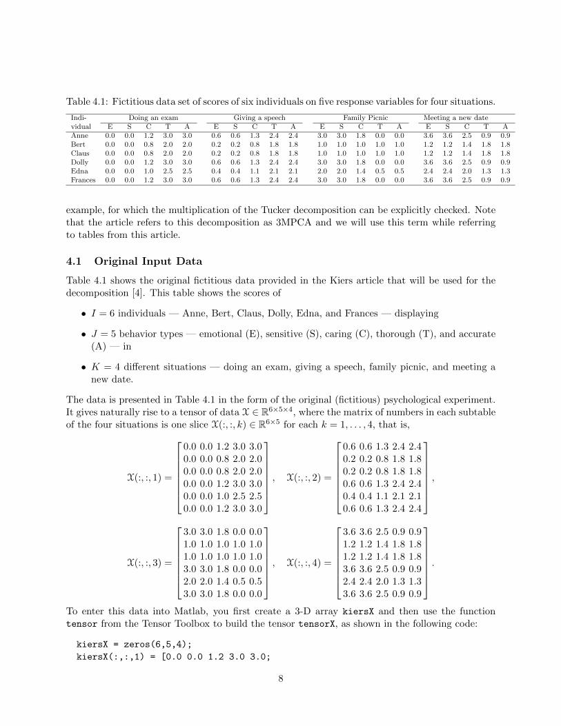
Table 4.1: Fictitious data set of scores of six individuals on five response variables for four situations.

Indi- Doing an exam Giving a speech Family Picnic Meeting a new datevidual E S C T A E S C T A E S C T A E S C T AAnne 0.0 0.0 1.2 3.0 3.0 0.6 0.6 1.3 2.4 2.4 3.0 3.0 1.8 0.0 0.0 3.6 3.6 2.5 0.9 0.9Bert 0.0 0.0 0.8 2.0 2.0 0.2 0.2 0.8 1.8 1.8 1.0 1.0 1.0 1.0 1.0 1.2 1.2 1.4 1.8 1.8Claus 0.0 0.0 0.8 2.0 2.0 0.2 0.2 0.8 1.8 1.8 1.0 1.0 1.0 1.0 1.0 1.2 1.2 1.4 1.8 1.8Dolly 0.0 0.0 1.2 3.0 3.0 0.6 0.6 1.3 2.4 2.4 3.0 3.0 1.8 0.0 0.0 3.6 3.6 2.5 0.9 0.9Edna 0.0 0.0 1.0 2.5 2.5 0.4 0.4 1.1 2.1 2.1 2.0 2.0 1.4 0.5 0.5 2.4 2.4 2.0 1.3 1.3Frances 0.0 0.0 1.2 3.0 3.0 0.6 0.6 1.3 2.4 2.4 3.0 3.0 1.8 0.0 0.0 3.6 3.6 2.5 0.9 0.9

example, for which the multiplication of the Tucker decomposition can be explicitly checked. Notethat the article refers to this decomposition as 3MPCA and we will use this term while referringto tables from this article.

4.1 Original Input Data

Table 4.1 shows the original fictitious data provided in the Kiers article that will be used for thedecomposition [4]. This table shows the scores of

• I = 6 individuals — Anne, Bert, Claus, Dolly, Edna, and Frances — displaying

• J = 5 behavior types — emotional (E), sensitive (S), caring (C), thorough (T), and accurate(A) — in

• K = 4 different situations — doing an exam, giving a speech, family picnic, and meeting anew date.

The data is presented in Table 4.1 in the form of the original (fictitious) psychological experiment.It gives naturally rise to a tensor of data X ∈ R6×5×4, where the matrix of numbers in each subtableof the four situations is one slice X(:, :, k) ∈ R6×5 for each k = 1, . . . , 4, that is,

X(:, :, 1) =

0.0 0.0 1.2 3.0 3.00.0 0.0 0.8 2.0 2.00.0 0.0 0.8 2.0 2.00.0 0.0 1.2 3.0 3.00.0 0.0 1.0 2.5 2.50.0 0.0 1.2 3.0 3.0

, X(:, :, 2) =

0.6 0.6 1.3 2.4 2.40.2 0.2 0.8 1.8 1.80.2 0.2 0.8 1.8 1.80.6 0.6 1.3 2.4 2.40.4 0.4 1.1 2.1 2.10.6 0.6 1.3 2.4 2.4

,

X(:, :, 3) =

3.0 3.0 1.8 0.0 0.01.0 1.0 1.0 1.0 1.01.0 1.0 1.0 1.0 1.03.0 3.0 1.8 0.0 0.02.0 2.0 1.4 0.5 0.53.0 3.0 1.8 0.0 0.0

, X(:, :, 4) =

3.6 3.6 2.5 0.9 0.91.2 1.2 1.4 1.8 1.81.2 1.2 1.4 1.8 1.83.6 3.6 2.5 0.9 0.92.4 2.4 2.0 1.3 1.33.6 3.6 2.5 0.9 0.9

.

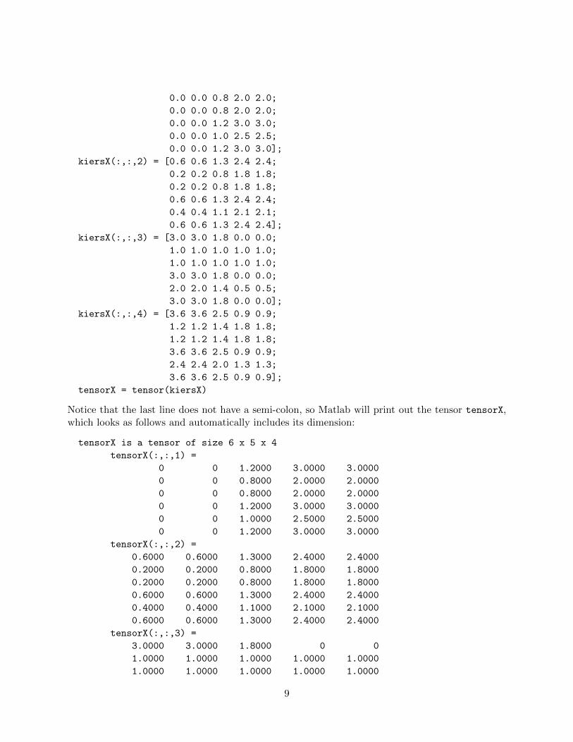
To enter this data into Matlab, you first create a 3-D array kiersX and then use the functiontensor from the Tensor Toolbox to build the tensor tensorX, as shown in the following code:

kiersX = zeros(6,5,4);

kiersX(:,:,1) = [0.0 0.0 1.2 3.0 3.0;

8

0.0 0.0 0.8 2.0 2.0;

0.0 0.0 0.8 2.0 2.0;

0.0 0.0 1.2 3.0 3.0;

0.0 0.0 1.0 2.5 2.5;

0.0 0.0 1.2 3.0 3.0];

kiersX(:,:,2) = [0.6 0.6 1.3 2.4 2.4;

0.2 0.2 0.8 1.8 1.8;

0.2 0.2 0.8 1.8 1.8;

0.6 0.6 1.3 2.4 2.4;

0.4 0.4 1.1 2.1 2.1;

0.6 0.6 1.3 2.4 2.4];

kiersX(:,:,3) = [3.0 3.0 1.8 0.0 0.0;

1.0 1.0 1.0 1.0 1.0;

1.0 1.0 1.0 1.0 1.0;

3.0 3.0 1.8 0.0 0.0;

2.0 2.0 1.4 0.5 0.5;

3.0 3.0 1.8 0.0 0.0];

kiersX(:,:,4) = [3.6 3.6 2.5 0.9 0.9;

1.2 1.2 1.4 1.8 1.8;

1.2 1.2 1.4 1.8 1.8;

3.6 3.6 2.5 0.9 0.9;

2.4 2.4 2.0 1.3 1.3;

3.6 3.6 2.5 0.9 0.9];

tensorX = tensor(kiersX)

Notice that the last line does not have a semi-colon, so Matlab will print out the tensor tensorX,which looks as follows and automatically includes its dimension:

tensorX is a tensor of size 6 x 5 x 4

tensorX(:,:,1) =

0 0 1.2000 3.0000 3.0000

0 0 0.8000 2.0000 2.0000

0 0 0.8000 2.0000 2.0000

0 0 1.2000 3.0000 3.0000

0 0 1.0000 2.5000 2.5000

0 0 1.2000 3.0000 3.0000

tensorX(:,:,2) =

0.6000 0.6000 1.3000 2.4000 2.4000

0.2000 0.2000 0.8000 1.8000 1.8000

0.2000 0.2000 0.8000 1.8000 1.8000

0.6000 0.6000 1.3000 2.4000 2.4000

0.4000 0.4000 1.1000 2.1000 2.1000

0.6000 0.6000 1.3000 2.4000 2.4000

tensorX(:,:,3) =

3.0000 3.0000 1.8000 0 0

1.0000 1.0000 1.0000 1.0000 1.0000

1.0000 1.0000 1.0000 1.0000 1.0000

9

3.0000 3.0000 1.8000 0 0

2.0000 2.0000 1.4000 0.5000 0.5000

3.0000 3.0000 1.8000 0 0

tensorX(:,:,4) =

3.6000 3.6000 2.5000 0.9000 0.9000

1.2000 1.2000 1.4000 1.8000 1.8000

1.2000 1.2000 1.4000 1.8000 1.8000

3.6000 3.6000 2.5000 0.9000 0.9000

2.4000 2.4000 2.0000 1.3000 1.3000

3.6000 3.6000 2.5000 0.9000 0.9000

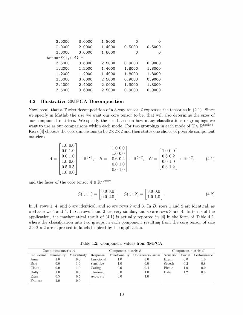
4.2 Illustrative 3MPCA Decomposition

Now, recall that a Tucker decomposition of a 3-way tensor X expresses the tensor as in (2.1). Sincewe specify in Matlab the size we want our core tensor to be, that will also determine the sizes ofour component matrices. We specify the size based on how many classifications or groupings wewant to use as our comparisons within each mode. For two groupings in each mode of X ∈ R6×5×4,Kiers [4] chooses the core dimensions to be 2×2×2 and then states one choice of possible componentmatrices

A =

1.0 0.00.0 1.00.0 1.01.0 0.00.5 0.51.0 0.0

∈ R6×2, B =

1.0 0.01.0 0.00.6 0.40.0 1.00.0 1.0

∈ R5×2, C =

1.0 0.00.8 0.20.0 1.00.3 1.2

∈ R4×2, (4.1)

and the faces of the core tensor G ∈ R2×2×2

G(:, :, 1) =

[0.0 3.00.0 2.0

], G(:, :, 2) =

[3.0 0.01.0 1.0

]. (4.2)

In A, rows 1, 4, and 6 are identical, and so are rows 2 and 3. In B, rows 1 and 2 are identical, aswell as rows 4 and 5. In C, rows 1 and 2 are very similar, and so are rows 3 and 4. In terms of theapplication, the mathematical result of (4.1) is actually reported in [4] in the form of Table 4.2,where the classification into two groups in each component resulting from the core tensor of size2× 2× 2 are expressed in labels inspired by the application.

Table 4.2: Component values from 3MPCA.

Component matrix A Component matrix B Component matrix CIndividual Femininity Masculinity Response Emotionality Conscientiousness Situation Social PerformanceAnne 1.0 0.0 Emotional 1.0 0.0 Exam 0.0 1.0Bert 0.0 1.0 Sensitive 1.0 0.0 Speech 0.2 0.8Claus 0.0 1.0 Caring 0.6 0.4 Picnic 1.0 0.0Dolly 1.0 0.0 Thorough 0.0 1.0 Date 1.2 0.3Edna 0.5 0.5 Accurate 0.0 1.0Frances 1.0 0.0

10

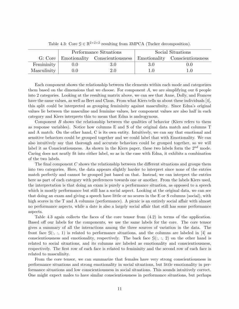
Table 4.3: Core G ∈ R2×2×2 resulting from 3MPCA (Tucker decomposition).

Performance Situations Social SituationsG: Core Emotionality Conscientiousness Emotionality Conscientiousness

Femininity 0.0 3.0 3.0 0.0Masculinity 0.0 2.0 1.0 1.0

Each component shows the relationship between the elements within each mode and categorizesthem based on the dimensions that we choose. For component A, we are simplifying our 6 peopleinto 2 categories. Looking at the resulting matrix above, we can see that Anne, Dolly, and Franceshave the same values, as well as Bert and Claus. From what Kiers tells us about these individuals [4],this split could be interpreted as grouping femininity against masculinity. Since Edna’s originalvalues lie between the masculine and feminine values, her component values are also half in eachcategory and Kiers interprets this to mean that Edna is androgynous.

Component B shows the relationship between the qualities of behavior (Kiers refers to themas response variables). Notice how columns E and S of the original data match and columns Tand A match. On the other hand, C is its own entity. Intuitively, we can say that emotional andsensitive behaviors could be grouped together and we could label that with Emotionality. We canalso intuitively say that thorough and accurate behaviors could be grouped together, so we willlabel it as Conscientiousness. As shown in the Kiers paper, these two labels form the 2nd mode.Caring does not neatly fit into either label, so as in the case with Edna, it exhibits a combinationof the two labels.

The final component C shows the relationship between the different situations and groups theminto two categories. Here, the data appears slightly harder to interpret since none of the entriesmatch perfectly and cannot be grouped just based on that. Instead, we can interpret the entrieshere as part of each category with preferences towards one or another. From the labels Kiers used,the interpretation is that doing an exam is purely a performance situation, as opposed to a speechwhich is mostly performance but still has a social aspect. Looking at the original data, we can seethat doing an exam and giving a speech have little or no scores in the E or S columns (social), withhigh scores in the T and A columns (performance). A picnic is an entirely social affair with almostno performance aspects, while a date is also a largely social affair that still has some performanceaspects.

Table 4.3 again collects the faces of the core tensor from (4.2) in terms of the application.Based off our labels for the components, we use the same labels for the core. The core tensorgives a summary of all the interactions among the three sources of variation in the data. Thefront face G(:, :, 1) is related to performance situations, and the columns are labeled in [4] asconscientiousness and emotionality, respectively. The back face G(:, :, 2) on the other hand isrelated to social situations, and its columns are labeled as emotionality and conscientiousness,respectively. The first row of each face is related to femininity and the second row of each face isrelated to masculinity.

From the core tensor, we can summarize that females have very strong conscientiousness inperformance situations and strong emotionality in social situations, but little emotionality in per-formance situations and low conscientiousness in social situations. This sounds intuitively correct.One might expect males to have similar conscientiousness in performance situations, but perhaps

11

less emotionality in social situations. We look back at the original data to see that females do havehigher scores on the conscientiousness responses (T and A) in the performance situations (Exam,Speech) and higher scores on the emotionality responses (E and S) in the social situations (Picnic,Date). Also in the original data, we note that the two males have lower scores on the conscien-tiousness responses (T and A) in the performance situations (Exam, Speech) and lower scores foremotionality responses (E and S) for social situations (Picnic and Date).

4.3 Verifying and Understanding Results

For clarity, we explain how to carry out the computations necessary to obtain the tensor thatcorresponds to the Kiers table displayed earlier. First, the multiplication with the tensor that istaking place is dependent on the mode being considered. The idea is that a tensor has 3 dimensions,or modes, and subscripts indicate the mode of multiplication considered when taking the productwith the factor matrices. For instance, mode-3 multiplication satisfies

Y = G×3 C ⇐⇒ Y(3) = CG(3)

where C ∈ RK×R, the G(3) ∈ RR×PQ, and Y(3) ∈ RK×PQ are mode-3 unfoldings of G ∈ RP×Q×R

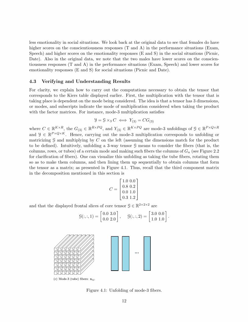
and Y ∈ RP×Q×K . Hence, carrying out the mode-3 multiplication corresponds to unfolding ormatricizing G and multiplying by C on the left (assuming the dimensions match for the productto be defined). Intuitively, unfolding a 3-way tensor G means to consider the fibers (that is, thecolumns, rows, or tubes) of a certain mode and making such fibers the columns of Gn (see Figure 2.2for clarification of fibers). One can visualize this unfolding as taking the tube fibers, rotating themso as to make them columns, and then lining them up sequentially to obtain columns that formthe tensor as a matrix; as presented in Figure 4.1. Thus, recall that the third component matrixin the decomposition mentioned in this section is

C =

1.0 0.00.8 0.20.0 1.00.3 1.2

and that the displayed frontal slices of core tensor G ∈ R2×2×2 are

G(:, :, 1) =

[0.0 3.00.0 2.0

], G(:, :, 2) =

[3.0 0.01.0 1.0

].

Figure 4.1: Unfolding of mode-3 fibers.

12

Since the mode-3 unfolding means we make the tube fibers of G into columns of the unfolded matrixG(3), then tube fibers can be thought of as columns going into the page (towards the other slices),so that we get

G(3) =

[0.0 3.0 0.0 2.03.0 0.0 1.0 1.0

]and the multiplication yields

Y(3) = CG(3) =

0.0 3.0 0.0 2.00.6 2.4 0.2 1.83.0 0.0 1.0 1.03.6 0.9 1.2 1.8

.

We can then follow this procedure for the other modes by unfolding the tensor represented by theseslices in the appropriate mode, so that one can carry out the multiplications in modes 1 and 2 withcomponent matrices A and B, respectively.

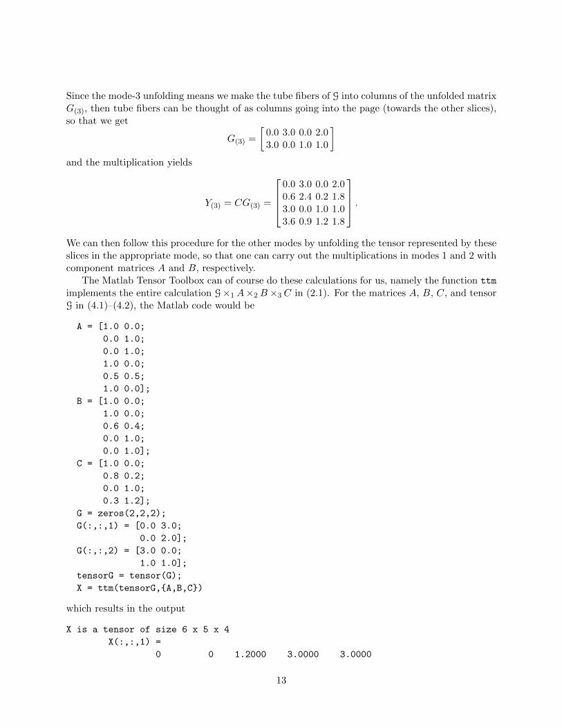
The Matlab Tensor Toolbox can of course do these calculations for us, namely the function ttm

implements the entire calculation G×1 A×2 B×3 C in (2.1). For the matrices A, B, C, and tensorG in (4.1)–(4.2), the Matlab code would be

A = [1.0 0.0;

0.0 1.0;

0.0 1.0;

1.0 0.0;

0.5 0.5;

1.0 0.0];

B = [1.0 0.0;

1.0 0.0;

0.6 0.4;

0.0 1.0;

0.0 1.0];

C = [1.0 0.0;

0.8 0.2;

0.0 1.0;

0.3 1.2];

G = zeros(2,2,2);

G(:,:,1) = [0.0 3.0;

0.0 2.0];

G(:,:,2) = [3.0 0.0;

1.0 1.0];

tensorG = tensor(G);

X = ttm(tensorG,{A,B,C})

which results in the output

X is a tensor of size 6 x 5 x 4

X(:,:,1) =

0 0 1.2000 3.0000 3.0000

13

0 0 0.8000 2.0000 2.0000

0 0 0.8000 2.0000 2.0000

0 0 1.2000 3.0000 3.0000

0 0 1.0000 2.5000 2.5000

0 0 1.2000 3.0000 3.0000

X(:,:,2) =

0.6000 0.6000 1.3200 2.4000 2.4000

0.2000 0.2000 0.8400 1.8000 1.8000

0.2000 0.2000 0.8400 1.8000 1.8000

0.6000 0.6000 1.3200 2.4000 2.4000

0.4000 0.4000 1.0800 2.1000 2.1000

0.6000 0.6000 1.3200 2.4000 2.4000

X(:,:,3) =

3.0000 3.0000 1.8000 0 0

1.0000 1.0000 1.0000 1.0000 1.0000

1.0000 1.0000 1.0000 1.0000 1.0000

3.0000 3.0000 1.8000 0 0

2.0000 2.0000 1.4000 0.5000 0.5000

3.0000 3.0000 1.8000 0 0

X(:,:,4) =

3.6000 3.6000 2.5200 0.9000 0.9000

1.2000 1.2000 1.4400 1.8000 1.8000

1.2000 1.2000 1.4400 1.8000 1.8000

3.6000 3.6000 2.5200 0.9000 0.9000

2.4000 2.4000 1.9800 1.3500 1.3500

3.6000 3.6000 2.5200 0.9000 0.9000

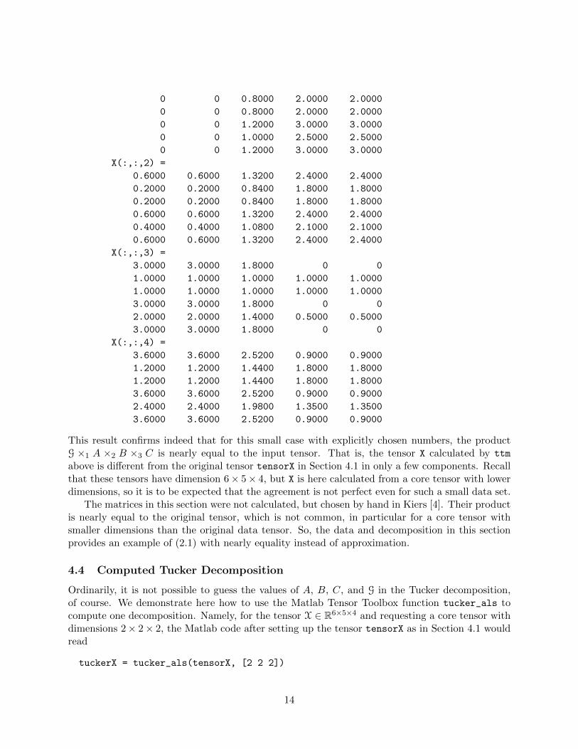
This result confirms indeed that for this small case with explicitly chosen numbers, the productG ×1 A ×2 B ×3 C is nearly equal to the input tensor. That is, the tensor X calculated by ttm

above is different from the original tensor tensorX in Section 4.1 in only a few components. Recallthat these tensors have dimension 6× 5× 4, but X is here calculated from a core tensor with lowerdimensions, so it is to be expected that the agreement is not perfect even for such a small data set.

The matrices in this section were not calculated, but chosen by hand in Kiers [4]. Their productis nearly equal to the original tensor, which is not common, in particular for a core tensor withsmaller dimensions than the original data tensor. So, the data and decomposition in this sectionprovides an example of (2.1) with nearly equality instead of approximation.

4.4 Computed Tucker Decomposition

Ordinarily, it is not possible to guess the values of A, B, C, and G in the Tucker decomposition,of course. We demonstrate here how to use the Matlab Tensor Toolbox function tucker_als tocompute one decomposition. Namely, for the tensor X ∈ R6×5×4 and requesting a core tensor withdimensions 2× 2× 2, the Matlab code after setting up the tensor tensorX as in Section 4.1 wouldread

tuckerX = tucker_als(tensorX, [2 2 2])

14

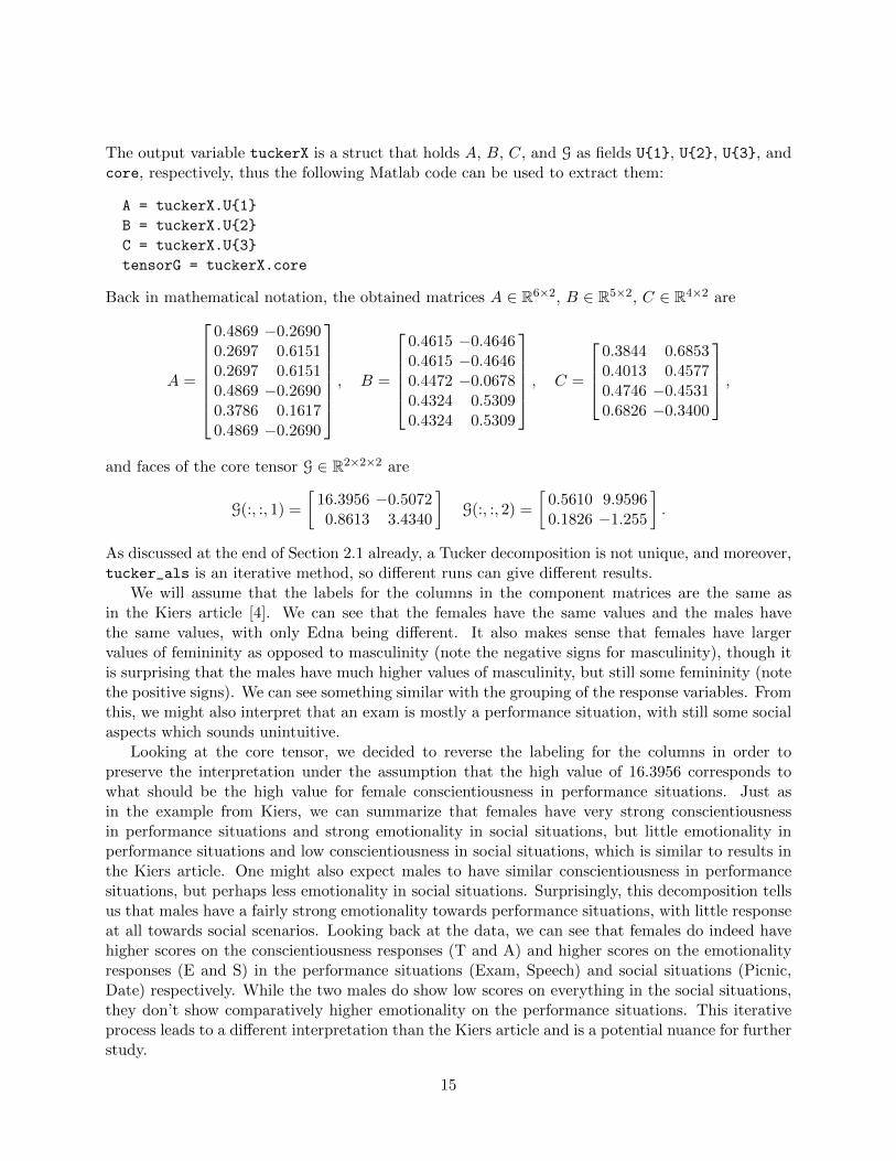
The output variable tuckerX is a struct that holds A, B, C, and G as fields U{1}, U{2}, U{3}, andcore, respectively, thus the following Matlab code can be used to extract them:

A = tuckerX.U{1}

B = tuckerX.U{2}

C = tuckerX.U{3}

tensorG = tuckerX.core

Back in mathematical notation, the obtained matrices A ∈ R6×2, B ∈ R5×2, C ∈ R4×2 are

A =

0.4869 −0.26900.2697 0.61510.2697 0.61510.4869 −0.26900.3786 0.16170.4869 −0.2690

, B =

0.4615 −0.46460.4615 −0.46460.4472 −0.06780.4324 0.53090.4324 0.5309

, C =

0.3844 0.68530.4013 0.45770.4746 −0.45310.6826 −0.3400

,

and faces of the core tensor G ∈ R2×2×2 are

G(:, :, 1) =

[16.3956 −0.50720.8613 3.4340

]G(:, :, 2) =

[0.5610 9.95960.1826 −1.255

].

As discussed at the end of Section 2.1 already, a Tucker decomposition is not unique, and moreover,tucker_als is an iterative method, so different runs can give different results.

We will assume that the labels for the columns in the component matrices are the same asin the Kiers article [4]. We can see that the females have the same values and the males havethe same values, with only Edna being different. It also makes sense that females have largervalues of femininity as opposed to masculinity (note the negative signs for masculinity), though itis surprising that the males have much higher values of masculinity, but still some femininity (notethe positive signs). We can see something similar with the grouping of the response variables. Fromthis, we might also interpret that an exam is mostly a performance situation, with still some socialaspects which sounds unintuitive.

Looking at the core tensor, we decided to reverse the labeling for the columns in order topreserve the interpretation under the assumption that the high value of 16.3956 corresponds towhat should be the high value for female conscientiousness in performance situations. Just asin the example from Kiers, we can summarize that females have very strong conscientiousnessin performance situations and strong emotionality in social situations, but little emotionality inperformance situations and low conscientiousness in social situations, which is similar to results inthe Kiers article. One might also expect males to have similar conscientiousness in performancesituations, but perhaps less emotionality in social situations. Surprisingly, this decomposition tellsus that males have a fairly strong emotionality towards performance situations, with little responseat all towards social scenarios. Looking back at the data, we can see that females do indeed havehigher scores on the conscientiousness responses (T and A) and higher scores on the emotionalityresponses (E and S) in the performance situations (Exam, Speech) and social situations (Picnic,Date) respectively. While the two males do show low scores on everything in the social situations,they don’t show comparatively higher emotionality on the performance situations. This iterativeprocess leads to a different interpretation than the Kiers article and is a potential nuance for furtherstudy.

15

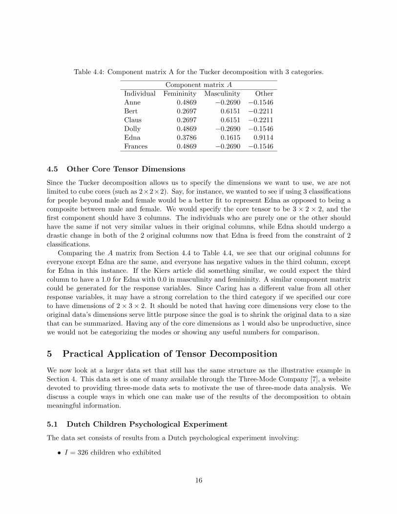
Table 4.4: Component matrix A for the Tucker decomposition with 3 categories.

Component matrix AIndividual Femininity Masculinity OtherAnne 0.4869 −0.2690 −0.1546Bert 0.2697 0.6151 −0.2211Claus 0.2697 0.6151 −0.2211Dolly 0.4869 −0.2690 −0.1546Edna 0.3786 0.1615 0.9114Frances 0.4869 −0.2690 −0.1546

4.5 Other Core Tensor Dimensions

Since the Tucker decomposition allows us to specify the dimensions we want to use, we are notlimited to cube cores (such as 2×2×2). Say, for instance, we wanted to see if using 3 classificationsfor people beyond male and female would be a better fit to represent Edna as opposed to being acomposite between male and female. We would specify the core tensor to be 3 × 2 × 2, and thefirst component should have 3 columns. The individuals who are purely one or the other shouldhave the same if not very similar values in their original columns, while Edna should undergo adrastic change in both of the 2 original columns now that Edna is freed from the constraint of 2classifications.

Comparing the A matrix from Section 4.4 to Table 4.4, we see that our original columns foreveryone except Edna are the same, and everyone has negative values in the third column, exceptfor Edna in this instance. If the Kiers article did something similar, we could expect the thirdcolumn to have a 1.0 for Edna with 0.0 in masculinity and femininity. A similar component matrixcould be generated for the response variables. Since Caring has a different value from all otherresponse variables, it may have a strong correlation to the third category if we specified our coreto have dimensions of 2× 3× 2. It should be noted that having core dimensions very close to theoriginal data’s dimensions serve little purpose since the goal is to shrink the original data to a sizethat can be summarized. Having any of the core dimensions as 1 would also be unproductive, sincewe would not be categorizing the modes or showing any useful numbers for comparison.

5 Practical Application of Tensor Decomposition

We now look at a larger data set that still has the same structure as the illustrative example inSection 4. This data set is one of many available through the Three-Mode Company [7], a websitedevoted to providing three-mode data sets to motivate the use of three-mode data analysis. Wediscuss a couple ways in which one can make use of the results of the decomposition to obtainmeaningful information.

5.1 Dutch Children Psychological Experiment

The data set consists of results from a Dutch psychological experiment involving:

• I = 326 children who exhibited

16

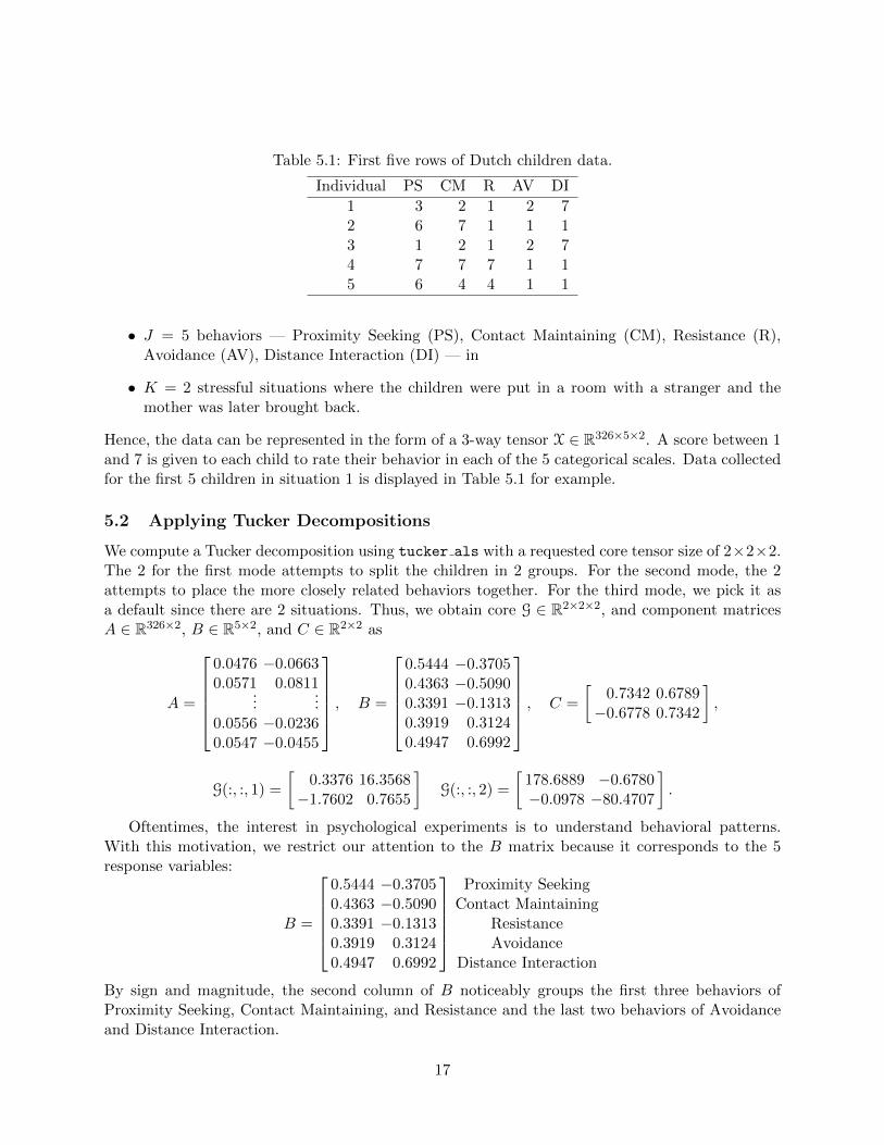
Table 5.1: First five rows of Dutch children data.

Individual PS CM R AV DI

1 3 2 1 2 72 6 7 1 1 13 1 2 1 2 74 7 7 7 1 15 6 4 4 1 1

• J = 5 behaviors — Proximity Seeking (PS), Contact Maintaining (CM), Resistance (R),Avoidance (AV), Distance Interaction (DI) — in

• K = 2 stressful situations where the children were put in a room with a stranger and themother was later brought back.

Hence, the data can be represented in the form of a 3-way tensor X ∈ R326×5×2. A score between 1and 7 is given to each child to rate their behavior in each of the 5 categorical scales. Data collectedfor the first 5 children in situation 1 is displayed in Table 5.1 for example.

5.2 Applying Tucker Decompositions

We compute a Tucker decomposition using tucker als with a requested core tensor size of 2×2×2.The 2 for the first mode attempts to split the children in 2 groups. For the second mode, the 2attempts to place the more closely related behaviors together. For the third mode, we pick it asa default since there are 2 situations. Thus, we obtain core G ∈ R2×2×2, and component matricesA ∈ R326×2, B ∈ R5×2, and C ∈ R2×2 as

A =

0.0476 −0.06630.0571 0.0811

......

0.0556 −0.02360.0547 −0.0455

, B =

0.5444 −0.37050.4363 −0.50900.3391 −0.13130.3919 0.31240.4947 0.6992

, C =

[0.7342 0.6789−0.6778 0.7342

],

G(:, :, 1) =

[0.3376 16.3568−1.7602 0.7655

]G(:, :, 2) =

[178.6889 −0.6780−0.0978 −80.4707

].

Oftentimes, the interest in psychological experiments is to understand behavioral patterns.With this motivation, we restrict our attention to the B matrix because it corresponds to the 5response variables:

B =

0.5444 −0.37050.4363 −0.50900.3391 −0.13130.3919 0.31240.4947 0.6992

Proximity Seeking

Contact MaintainingResistanceAvoidance

Distance Interaction

By sign and magnitude, the second column of B noticeably groups the first three behaviors ofProximity Seeking, Contact Maintaining, and Resistance and the last two behaviors of Avoidanceand Distance Interaction.

17

We project the first 5 children’s data onto the second column of B. In other words, we take thedot product of each row of the children’s data with the second column of B and get

X(1 :5, : , 1)B(: , 2) =

3 2 1 2 76 7 1 1 11 2 1 2 77 7 7 1 16 4 4 1 1

−0.3705−0.5090−0.1313

0.31240.6992

=

3.2583−4.0955

3.9993−6.0638−3.7725

.

Negative values correspond to the extent to which behaviors of Proximity Seeking and/or ContactMaintaining are present. Positive values correspond to the extent to which behaviors of Avoidanceand/or Distance Interaction are present. This projection helps summarize information about thebehavior of each child in situation 1.

The Tensor Toolbox allows us to request different tensor core sizes. For further exploration,we compute a Tucker decomposition by requesting a core tensor of size 2× 3× 2, which results incomponent matrices A ∈ R326×2, B ∈ R5×3, C ∈ R2×2, and core tensor G ∈ R2×3×2

A =

0.0476 −0.06670.0570 0.0807

......

0.0552 −0.02400.0546 −0.0458

, B =

0.5444 −0.3706 0.64700.4363 −0.5084 −0.55730.3391 −0.1316 −0.31010.3919 0.3111 0.32380.4947 0.7001 −0.2643

, C =

[0.7342 0.6790−0.6790 0.7342

],

G(:, :, 1) =

[0.3369 16.3405 4.6376−1.7663 0.7502 1.3683

], G(:, :, 2) =

[178.6895 −0.0863 0.0055−0.1397 −80.4702 0.9545

].

We also compute a Tucker decomposition for a core tensor of size 2×4×2, which gives componentmatrices A ∈ R326×2, B ∈ R5×4, C ∈ R2×2, and core tensor G ∈ R2×4×2

A =

0.0476 −0.06630.0570 0.0809

......

0.0552 −0.02420.0546 −0.0456

, B =

0.5444 −0.3713 0.6499 −0.00870.4363 −0.5086 −0.5581 −0.45550.3391 −0.1305 −0.3113 0.87600.3919 0.3128 0.3178 −0.04830.4947 0.6990 −0.2612 −0.1509

, C =

[0.7342 0.6789−0.6789 0.7342

],

G(:, :, 1) =

[0.3446 16.3399 4.6349 −0.4621−1.7529 0.7657 1.3615 1.6279

], G(:, :, 2) =

[178.6896 −0.0853 0.0051 0.0168−0.1362 −80.4694 0.9541 −0.0784

].

In this instance, the first and second columns of B do not drastically change across the differentsizes of the core tensor.

It is important to note at this point that we have performed a similar decomposition on twodifferent sets of data, but used them for different methods of interpretation. With the Kiers article,the decomposition was used to show how all of the components related to each other and is anillustrative example on how to label the columns given that the properties of the individuals areknown. For the Dutch experiment, we chose to only focus on the B matrix that corresponded to theresponse variables. Due to the similarity of sign and magnitude of the first column in B, we choseto focus on the second column. We have extended the analysis done with Tucker by projectingthe rows of the original data onto the second column of the second component matrix B. Doingthis allowed us to provide a summary of the children’s behavioral tendencies. How one chooses toanalyze and interpret the results depends on the data that is being used as well as what the userwants to look for.

18

6 Conclusions

Data can exist in more than two dimensions and tensor decompositions allow us to directly per-form analysis on this multi-dimensional data, as opposed to performing multiple analyses on two-dimensional data through techniques such as principal component analysis (PCA). We consideredtwo examples from psychological studies due to their intuitive nature, one small and one modestsized one. We showed the details of commands from the Matlab Tensor Toolbox needed to set upand analyze them.

The Matlab Tensor Toolbox (version 2.6) was able to do the calculations for the small amountof data in the examples of Sections 4 and 5 in seconds. This suggests it might do well with largerdata sets, and highlights that other programming languages like C might be able to handle evenlarger computations. Using these tools, there is a wide range of potential applications for multi-dimensional data such as signals analytics, facial recognition, big-data analysis, etc. with muchlarger datasets.

Acknowledgments

These results were obtained as part of the REU Site: Interdisciplinary Program in High PerformanceComputing (hpcreu.umbc.edu) in the Department of Mathematics and Statistics at the Universityof Maryland, Baltimore County (UMBC) in Summer 2016. This program is funded by the NationalScience Foundation (NSF), the National Security Agency (NSA), and the Department of Defense(DOD), with additional support from UMBC, the Department of Mathematics and Statistics, theCenter for Interdisciplinary Research and Consulting (CIRC), and the UMBC High PerformanceComputing Facility (HPCF). HPCF is supported by the U.S. National Science Foundation throughthe MRI program (grant nos. CNS–0821258 and CNS–1228778) and the SCREMS program (grantno. DMS–0821311), with additional substantial support from UMBC. Co-author Darren Stevens IIwas supported, in part, by the UMBC National Security Agency (NSA) Scholars Program througha contract with the NSA. The authors thank both our team’s graduate assistant Jonathan Graf andfaculty mentor Dr. Matthias K. Gobbert for their support throughout the program and beyond,and we are grateful to the project client Dr. Tyler Simon from the Laboratory for Physical Sciencesfor pointing us to the interesting issue of tensor analysis and the Matlab Tensor Toolbox.

References

[1] E. Acar, D. M. Dunlavy, and T. G. Kolda, Link prediction on evolving data using matrixand tensor factorizations, in 2009 IEEE International Conference on Data Mining Workshops,Dec. 2009, pp. 262–269.

[2] D. Fitzgerald, E. Coyle, and M. Cranitch, Using tensor factorisation models to separatedrums from polyphonic music, in Proceedings of the International Conference on Digital AudioEffects (DAFX09), 2009.

[3] U. Kang, E. Papalexakis, A. Harpale, and C. Faloutsos, Gigatensor: Scaling ten-sor analysis up by 100 times — algorithms and discoveries, in Proceedings of the 18th ACMSIGKDD International Conference on Knowledge Discovery and Data Mining, KDD ’12, ACM,2012, pp. 316–324.

19

[4] H. A. L. Kiers and I. V. Mechelen, Three-way component analysis: Principles and illus-trative application, Psychological Methods, 6 (2001), pp. 84–110.

[5] T. G. Kolda and B. W. Bader, Tensor decompositions and applications, SIAM Review, 51(2009), pp. 455–500.

[6] T. G. Kolda and J. Sun, Scalable tensor decompositions for multi-aspect data mining, in2008 Eighth IEEE International Conference on Data Mining, Dec. 2008, pp. 363–372.

[7] P. M. Kroonenberg, The Three-Mode Company. http://three-mode.leidenuniv.nl. Ac-cessed September 12, 2016.

[8] E. E. Papalexakis, U. Kang, C. Faloutsos, N. D. Sidiropoulos, and A. Harpale,Large scale tensor decompositions: Algorithmic developments and applications, IEEE Data En-gineering Bulletin, 36 (2013), pp. 59–66.

20