Functions

Definitions and VocabularyA function 𝑓: 𝐴 → 𝐵 is a rule that assigns to each element of the set 𝐴 exactly one element in the set 𝐵. 𝑓 is the name of the function. We write 𝑓 𝑥 = 𝑦 to denote that 𝑓 assigns the element 𝑦 ∈ 𝐵 to the element 𝑥 ∈ 𝐴, and we refer to 𝑥 as an input, and to 𝑦 as an output. We also say that 𝑦 is the image of 𝑥under f, and that 𝑥 is a preimage of 𝑦 under f.

The set of inputs 𝐴 is called the domain of the function. The definition of function allows for the function to only assign a proper subset of elements of 𝐵 to elements of 𝐴. Therefore, 𝐵 is not the set of outputs, it is only a set of potential outputs. We call 𝐵 the codomain.

The set of actual outputs is called the range of the function:

range 𝑓 = 𝑦 ∈ 𝐵 ∃𝑥 ∈ 𝐴 𝑓 𝑥 = 𝑦 ⊆ codomain 𝑓We also say that 𝑓 maps 𝐴 to 𝐵, and refer to 𝑓 as a map.

Two functions 𝑓 , 𝑔 are equal if and only if their domains are equal, their codomains are equal, and 𝑓 𝑥 = 𝑔(𝑥) for all 𝑥 in the common domain.

Range vs CodomainBeginners often confuse range and codomain, or understand the concept, but don’t see why we need the concept of codomain.It is helpful to explain the difference with a programming analogy: the codomain corresponds to the output data type of the function. For example, the following C function always outputs a long. That makes long, interpreted as a set, the codomain:

long sqr(int n) {

return n*n;

}

That does not mean, however, that every possible long will actually be produced as an output of that function, i.e be in the range. In fact, most long values will never occur as outputs, namely those longs that are negative, or not perfect squares (2,3,5, etc).

Determining the exact range requires knowledge of the domain. In C, a standard int is an integer in [-32767, 32767]. The square of such a number is at most 1,073,676,289 (which fits comfortably into a long value). Therefore, the range is { 0, 1, 4, 9, 25, 36, …, 1073676289 }.

Knowing this range is important, because it helps us identify what operations we can perform on an output of this function. For example, taking sqr(n), subtracting 1073676289 and then taking the reciprocal would not always produce a numerical value, so a program that makes that assumption would behave in unexpected ways or crash – but only for two n values out of 65534. Casual testing might never uncover this problem.

Why should I care about theoretical issues like domain and range? I’m not

studying to be a mathematician! The previous page should already have given you an answer: domain and range considerations are critical for program correctness. Failure to take domain and range properly into account can be a costly mistake: In 1996, the first Ariane 5 rocket exploded 30 seconds after lift-off due to loss of guidance, caused by a software exception in the rocket’s inertial reference system during the conversion of a 64 bit floating point value into a 16 bit signed integer value. The conversion failed because the 64 bit floating point value, which was related to the rocket’s horizontal velocity, was outside the range expected by the designers of the software.

One careless coding decision caused $500M in damage and a setback for Europe’s space program.

When you don’t pay close attention to domain and range, rockets may explode, trains collide, and bridges collapse. Considering that our civilization is getting ever more dependent on software, the end of human civilization may well be caused not by nuclear war, or a cataclysmic plague, or an asteroid impact. It may be caused by a coder whose mindset is that “domain and range are for mathematicians in their ivory towers, not for people who work in the real world”. Don’t be that person.

Representing FunctionsFunctions that have a finite domain can be represented by a table of values or an arrow diagram.

For the function on the right, the domain is 𝐴 ={1,2,3,4} and the codomain is 𝐵 = {1,4,7}.

We could have defined the function by stating that 𝑓 1 = 4, 𝑓 2 = 7, 𝑓 3 = 1 and 𝑓 4 = 1.

Observe that the definition of a function does notrequire that the action of the function can be summarized by a formula. There is no obvious algebraic expression that would reproduce the outputs of our example function 𝑓, yet 𝑓 is a valid function.

Also observe that while a function can only assign one output to each input, one element in the codomain may well be the output of more than one input.

𝒙 𝒇(𝒙)

1 4

2 7

3 1

4 1

Representing Functions AlgebraicallyMany important functions have an algebraic definition: how to get the output from the input is described by a (perhaps piecewise) algebraic expression. Mathematics users frequently omit explicit specification of domain and codomain, and do not bother with quantifiers. For example, it is customary to define a function by writing

𝑓 𝑥 = 𝑥2

without bothering to define domain and codomain, and to mention that this definition is for all (rather than just for some) numbers 𝑥.

The convention is that when the domain is not specified, it defaults to the largest set of real numbers 𝑥 for which the expression 𝑓(𝑥) is defined- in this case, all real numbers. The default codomain for a real-valued function is always all real numbers.

A precise mathematical definition of the function above would be

𝑓:ℝ → ℝ; 𝑓 𝑥 = 𝑥2 for all 𝑥 ∈ ℝ.

Well-Definedness

A function is defined by its domain and codomain, and by how you find the output corresponding to each input. These pieces of information are not entirely independent of each other. Simply by defining the domain and by specifying the outputs for the inputs, you have already constrained the codomain – the codomain must at least contain the outputs. If you formally specify a codomain that does not contain all the outputs, then your definition of the function is inconsistent. In that case, we say that the function is not well-defined.

Example: 𝑓: 0,1 → 0,1 , 𝑓 𝑥 = 𝑥2 + 1 is not well-defined because 𝑥2 + 1assumes values ranging from 1 to 2 if you evaluate it on the interval 0,1 . To make the function well-defined, we should change the codomain to 1,2 , or any superset of that.

To avoid this problem altogether, people often just make an “obviously correct” choice for the codomain, such as ℝ for a function that produces only real numbers.

Floor and Ceiling FunctionsInformally, the floor function rounds down and the ceiling function rounds up. More precisely, if 𝑥 is a real number, then the floor of 𝑥, written 𝑥 is the greatest integer that is not greater than 𝑥, and the ceiling of 𝑥, written 𝑥 , is the smallest integer that is not smaller than 𝑥.

Examples:2.1 = 2

−1.3 = −22.1 = 3

−1.3 = −1

It follows from the definition (and geometrically from the graphs shown on the right) that the inequalities

𝑥 − 1 < 𝑥 ≤ 𝑥

𝑥 ≤ 𝑥 < 𝑥 + 1

hold for all real numbers 𝑥. Image Source: Wikimedia Commons, licensed for free public use.

Some cautionary notes on the floor and ceiling functions

You must be careful when you manipulate algebraic expressions involving floor and ceilings. For example, the following equations are not identities, i.e. not universallytrue:

𝑥 + 𝑦 = 𝑥 + 𝑦 , 𝑥𝑦 = 𝑥 𝑦

You solve equations that give you the floor or ceiling of a function by transforming the given equality into an equivalent double inequality. For example, the equality 2𝑥 + 5 = 10 is equivalent to

10 ≤ 2𝑥 + 5 < 11.

[This rule is a consequence of the inequalities given on the previous page. You should fill in the details as an exercise.]

The Image Function on SetsGiven a function 𝑓: 𝐴 → 𝐵 and a set of inputs 𝑋 ⊆ 𝐴, we define the f-image of 𝑋, or just the image of 𝑋, written 𝑓(𝑋) to be the set of all outputs of the inputs in 𝑋:

𝑓 𝑋 = 𝑓 𝑥 𝑥 ∈ 𝑋For example, if 𝑓 is the square function,

𝑓:ℝ → ℝ; 𝑓 𝑥 = 𝑥2 for all 𝑥 ∈ ℝ

then the image of the interval [0,2] is 𝑓 0,2 = 0,4 .

This assignment of a set of outputs to a set of inputs is technically a new and differentfunction, because it is a function from the set of all subsets of 𝐴, which is the power set of 𝐴, to the set of all subsets of 𝐵, which is the power set of 𝐵:

𝑓:𝒫 𝐴 → 𝒫 𝐵

It would be appropriate to give this new function a different name, but it is tradition that it be called 𝑓 just like the original function𝑓: 𝐴 → 𝐵 it is based on.

The Preimage Function

Given a function 𝑓: 𝐴 → 𝐵 and a set of potential outputs 𝑌 ⊆ 𝐵, we define the f-preimage of 𝑌, or just the preimage of 𝑌, written 𝑓−1(𝑌) to be the set of inputs whose outputs lie in 𝑌:

𝑓−1(𝑌) = 𝑥 ∈ 𝐴 𝑓(𝑥) ∈ 𝑌Note that this "𝑓−1“ is not the inverse function. 𝑓 may not even have an inverse, but the preimage function𝑓−1: 𝒫 𝐵 → 𝒫 𝐴 always exists.

For example, if 𝑓 is again the square function like in the previous slide, then the preimage of the interval [0,4] is

𝑓−1 0,4 = [−2,2]

Observe that the preimage gathers ALL inputs that lead to the given set of outputs, not just some of them. While it is true that the numbers in the interval [0,2] would be sufficient to create the numbers in the interval [0,4] as outputs, the preimage of [0,4] includes all numbers whose output lie in that interval, including the ones in [-2, 0).

Example: Images and Preimages of a Function that Involves the Floor

Suppose 𝑓 𝑥 =1

2𝑥 − 1 for all real numbers 𝑥. Find 𝑓−1 {4} and 𝑓 [3,5] .

This first part asks us to find all inputs 𝑥 such that 1

2𝑥 − 1 = 4. By definition

of floor, this is equivalent to 4 ≤1

2𝑥 − 1 < 5, which is in turn equivalent to

10 ≤ 𝑥 < 12. Therefore, 𝑓−1 {4} = [10,12).

The second part asks us to determine what happens if 𝑓 is applied to all 𝑥 ∈3,5 . If 3 ≤ 𝑥 ≤ 5, then

1

2≤

1

2𝑥 − 1 ≤

3

2, which implies 0 ≤

1

2𝑥 − 1 ≤ 1.

Therefore, 1

2𝑥 − 1 can only be 0 or 1.

Thus 𝑓 [3,5] ⊆ 0,1 . Evaluating 𝑓 3 = 0 and 𝑓 5 = 1 shows

0,1 ⊆ 𝑓 [3,5] . Thus, 𝑓 [3,5] = 0,1 .

Injective or one-to-one functionsSome functions map two or more different inputs to the same output. Such functions could be called information degrading because the knowledge of an output is not sufficient to reconstruct the input that lead to it. This can be undesirable in applications.

For example, there is a function that assigns to each ASU student a number called their ASU ID number. It encodes the identity of each student as a number. This function must not be information degrading, because the identity of the student must be recoverable from the ID number. Two students cannot share the same ID.

A function that is not information degrading , that assigns each output to only one input is called injective or 1-1. The formal definition is:

𝑓: 𝐴 → 𝐵 is called injective or one-to-one (or just “1-1”) iff

∀𝑥1, 𝑥2 ∈ 𝐴(𝑓 𝑥1 = 𝑓 𝑥2 → 𝑥1 = 𝑥2)

In words, two outputs of an injective function can only be the same if the two inputs were the same. (We may omit the domain specification “∈ 𝐴” from the statement above, since 𝐴 is the default domain.)

Why should I care about a theoretical property like injectivity? I’m not studying to be a mathematician!

Unique identifiers are a backbone of the information age – for good and for bad. They are needed so that law enforcement IT systems will know that you are not the same Joe Miller as the one who just committed an armed robbery in your town. They are needed so when you order a copy of the unabridged, hardcover 1946 edition of Ulysses, you don’t get the 2014 paperback edition. They are needed so that the pharmacy knows that you are the Jane Smith who is picking up an antibiotic, not the Jane Smith who is picking up an antidepressant.

The functions that compute unique identifiers need to be injective in principle. Injectivity is just a fancy name for uniqueness of outputs. Failure to design such a function properly can have adverse consequences to life, liberty and happiness. Such failure can cause you to receive an item you didn’t order; it can cause the wrong Joe Miller to be arrested or lose his voting rights; and it can cause Jane Smith to die from trivial illness.

Proving that a function is injective

Our knowledge of the graph of a function often allows us determine instantly that the function is injective. For example, we know that the graph of the function 𝑓 𝑥 = 3𝑥 + 1 is a straight line with a positive slope. Therefore, we recognize that the function cannot repeat outputs.

Such intuitive identification is not proof however. A proof of injectivity requires us to prove that the statement

∀𝑥1, 𝑥2(𝑓 𝑥1 = 𝑓 𝑥2 → 𝑥1 = 𝑥2)is true.

Proposition: the function 𝑓:ℝ → ℝ; 𝑓 𝑥 = 3𝑥 + 1 for all 𝑥 ∈ ℝ, is injective.

Proof: Suppose 𝑥1 and 𝑥2 are real numbers with 𝑓 𝑥1 = 𝑓(𝑥2). Then by definition of 𝑓, that means 3𝑥1 + 1 = 3𝑥2 + 1. By subtracting 1 from both sides and then dividing by 3, we obtain 𝑥1 = 𝑥2.

Proving that a function is not injective

To prove a universally quantified statement wrong, we only need to produce one (set of) value(s) that make the statement false. To prove that a function is not injective, i.e. to prove that

∀𝑥1, 𝑥2(𝑓 𝑥1 = 𝑓 𝑥2 → 𝑥1 = 𝑥2)

is a false statement, we just need to find one pair of numbers 𝑥1, 𝑥2 that makes the conditional 𝑓 𝑥1 = 𝑓 𝑥2 → 𝑥1 = 𝑥2 false. This means that we need to find two different inputs 𝑥1, 𝑥2 that share the same output so that the premise 𝑓 𝑥1 = 𝑓 𝑥2is true but the conclusion 𝑥1 = 𝑥2 is false.

Let us prove that the function

𝑓:ℝ → ℝ; 𝑓 𝑥 = 𝑥2 for all 𝑥 ∈ ℝ

is not injective. We have reason to believe that it is not injective, because its graph is a parabola, which is symmetric with respect to the y axis and therefore produces each output twice.

To prove non-injectivity, we simply observe 𝑓 −1 = 𝑓(1). That completes the proof.

Making a function injective by restricting its domain

We can always force a non-injective function to become injective by restricting its domain to a suitable subset to avoid repetition of outputs. For example, the square function becomes injective if we restrict it to the non-negative real numbers.

Proposition: 𝑓: [0,∞) → [0,∞); 𝑓 𝑥 = 𝑥2 is injective.

Proof: : Suppose 𝑥1 and 𝑥2 are non-negative real numbers with 𝑓 𝑥1 = 𝑓(𝑥2). Then by definition of 𝑓, that means 𝑥1

2 = 𝑥22, which implies 𝑥1

2 − 𝑥22 = 𝑥1 + 𝑥2 (

)𝑥1 −

𝑥2 = 0. Hence, 𝑥1 + 𝑥2 = 0 or 𝑥1 − 𝑥2 = 0, which implies 𝑥1 = −𝑥2 or 𝑥1 = 𝑥2.

Case 1: 𝑥1 = −𝑥2. Since 𝑥1 and 𝑥2 are both assumed non-negative, 𝑥1 ≥ 0 and −𝑥2 ≤0. Therefore, 𝑥1 = −𝑥2 if and only if 𝑥1 = −𝑥2 = 0. In that case, 𝑥1 = 𝑥2.

Case 2: 𝑥1 = 𝑥2. There is nothing more to do in this case.

In either case, we have 𝑥1 = 𝑥2.

[Note: applying the square root function to 𝑥12 = 𝑥2

2 is not a valid proof technique because it assumes the conclusion. Details are explained on the page titled “We must not inadvertently assume the conclusion when we prove injectivity”.]

Surjective or Onto FunctionsThe definition of a function does not require the codomain to be equal to the range. This is practical because the range of a function is not always obvious. No one can see just by looking at it what the range of, say,

𝑓 𝑥 = 𝑥4 − 𝑥2 + 𝑥

might be. Rules from Calculus I tell us that this function goes to infinity on the right and left, and therefore has an absolute minimum c. Since it is also continuous, its range is 𝑐,∞ , but determining the value of c requires some labor.

In those cases however when the range equals the codomain, in other words, when the codomain has been optimally chosen to be the smallest possible set it could be, we call the function surjective or onto. The technical definition of surjectivity is:

𝑓: 𝐴 → 𝐵 is called surjective or onto iff ∀𝑦 ∈ 𝐵 ∃𝑥 ∈ 𝐴(𝑓 𝑥 = 𝑦).

It is common to declare that a function 𝑓: 𝐴 → 𝐵 is onto by saying that 𝑓 is a function from 𝐴 onto 𝐵.

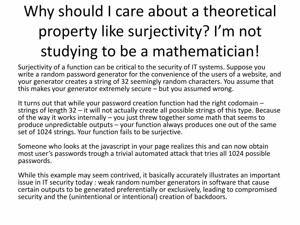
Why should I care about a theoretical property like surjectivity? I’m not studying to be a mathematician!

Surjectivity of a function can be critical to the security of IT systems. Suppose you write a random password generator for the convenience of the users of a website, and your generator creates a string of 32 seemingly random characters. You assume that this makes your generator extremely secure – but you assumed wrong.

It turns out that while your password creation function had the right codomain –strings of length 32 – it will not actually create all possible strings of this type. Because of the way it works internally – you just threw together some math that seems to produce unpredictable outputs – your function always produces one out of the same set of 1024 strings. Your function fails to be surjective.

Someone who looks at the javascript in your page realizes this and can now obtain most user’s passwords trough a trivial automated attack that tries all 1024 possible passwords.

While this example may seem contrived, it basically accurately illustrates an important issue in IT security today : weak random number generators in software that cause certain outputs to be generated preferentially or exclusively, leading to compromised security and the (unintentional or intentional) creation of backdoors.

Proving that a function is surjective

Even though knowledge of the graph can quickly convince us that a function must be surjective, proving that requires us to verify the condition

∀𝑦 ∈ 𝐵 ∃𝑥 ∈ 𝐴(𝑓 𝑥 = 𝑦)

This is a “for all, there exists” type of condition and must therefore be proved in the fashion we studied in an earlier presentation: for each arbitrary 𝑦 ∈ 𝐵, we must find the 𝑥 ∈ 𝐴 so that 𝑓 𝑥 = 𝑦 is satisfied. In practice, we do this by solving the equation 𝑓 𝑥 = 𝑦 for 𝑥. Let us discuss an example of such a proof.

Proposition: the function 𝑓:ℝ → ℝ; 𝑓 𝑥 = 3𝑥 + 1 is surjective.

Proof: assume 𝑦 is a real number. Let 𝑥 =𝑦−1

3. Then 𝑥 is a real number and therefore

in the domain of 𝑓. Then we can apply 𝑓 to 𝑥 and get

𝑓 𝑥 = 3𝑦 − 1

3+ 1 = 𝑦

That completes the proof.

Proving that a function is not surjective

To prove that a function is not surjective, we need to find a potential output 𝑦(an element of the codomain) that is not an actual output (not in the range). To show that 𝑦 is not in the range means showing that 𝑦 is unequal to 𝑓 𝑥for every 𝑥 in the domain.

Formally, we arrive at the same method for proving a function non-surjective by considering the negation of the condition for surjectivity,

¬ ∀𝑦 ∈ 𝐵 ∃𝑥 ∈ 𝐴 𝑓 𝑥 = 𝑦 = ∃𝑦 ∈ 𝐵∀𝑥 ∈ 𝐴 𝑓 𝑥 ≠ 𝑦

Let us verify this condition for the square function.

Proposition: 𝑓:ℝ → ℝ; 𝑓 𝑥 = 𝑥2 is not surjective.

Proof: let 𝑦 = −1. Since 𝑓 𝑥 = 𝑥2 ≥ 0 for all 𝑥 ∈ ℝ, 𝑓 𝑥 ≠ 𝑦 for all 𝑥 ∈ ℝ. That completes the proof.

Making a non-surjective function surjective

By changing the codomain of a non-surjective function to the range, we force the function to become surjective. (Technically, we are creating a different function by changing the codomain, but the new function is for all practical intents and purposes equal to the old function.)

For example, 𝑓:ℝ → ℝ; 𝑓 𝑥 = |𝑥| is not surjective, because negative real numbers do not occur as outputs of 𝑓.

However, 𝑔:ℝ → [0,∞); 𝑔 𝑥 = |𝑥| is surjective.

Proof: Assume 𝑦 is a member of the codomain of 𝑔, i.e. a non-negative real number. Since 𝑦 is a real number, it is in the domain of 𝑔, which means that we can apply 𝑔 to it. We get 𝑔 𝑦 = 𝑦 = 𝑦.

Visualizing Injectivity and Surjectivity

BijectivityA function that is injective and surjective (one-to-one and onto) is called bijective or a bijection. Examples of bijective functions:

𝑓:ℝ → ℝ; 𝑓 𝑥 = 3𝑥 + 1 𝑔: 0,∞ → 0,∞ ; 𝑔 𝑥 = 𝑥2

ℎ: −𝜋

2,𝜋

2→ −1,1 ; ℎ 𝑥 = sin 𝑥 𝑘: ℤ → ℤ; 𝑘 𝑥 = 𝑥 = 𝑥

Each bijective function 𝑓: 𝐴 → 𝐵 is invertible, meaning it has an inverse function𝑓−1: 𝐵 → 𝐴. The inverse function “reverses” the action of the function 𝑓: for all y ∈ 𝐵,𝑓−1(𝑦) is the unique 𝑥 ∈ 𝐴 that has the property 𝑓 𝑥 = 𝑦.

The technical definition of the inverse is the following: given 𝑓: 𝐴 → 𝐵, a function 𝑔: 𝐵 → 𝐴 is called the inverse of 𝑓, written 𝑓−1, if and only if 𝑓 𝑔 𝑥 = 𝑥 for all 𝑥 ∈𝐵 and 𝑔 𝑓 𝑥 = 𝑥 for all 𝑥 ∈ 𝐴.

Observe that the concept of the inverse function requires 𝑓 to be both one-to-one and onto. Without 𝑓 being onto, the 𝑥 ∈ 𝐴 with 𝑓 𝑥 = 𝑦 would not exist for every y ∈ 𝐵, and without 𝑓 being one-to-one, it would not always be unique.

You should convince yourself that the following is true: if 𝑓: 𝐴 → 𝐵 is bijective and 𝑌 ⊆𝐵, then the two possible interpretations of the symbol 𝑓−1(𝑌) agree. The 𝑓-preimage of 𝑌 and the 𝑓−1-image of 𝑌 are the same set.

An Example of Bijectivity

Prove that the function 𝑓: 4,7 → 2,3 , 𝑓 𝑥 =1

3𝑥 − 1 + 1 is bijective.

First we might want to convince ourselves that 𝑓 is well-defined in the first place, i.e. that the specified codomain contains all the outputs. Formally, we must show ∀𝑥(𝑥 ∈4,7 → 𝑓(𝑥) ∈ 2,3 ).

Suppose 𝑥 ∈ 4,7 . By definition of a closed interval, that means 4 ≤ 𝑥 ≤ 7. That implies 3 ≤ 𝑥 − 1 ≤ 6, which in turn implies 1 ≤

1

3𝑥 − 1 ≤ 2. Therefore, 2 ≤

1

3𝑥 − 1 + 1 = 𝑓 𝑥 ≤ 3.

Having thus proved that 𝑓 is well-defined, we prove that 𝑓 is injective: Suppose 𝑓 𝑎 = 𝑓(𝑏) for some 𝑎, 𝑏 ∈ 4,7 . By applying the definition of 𝑓, we get

1

3𝑎 − 1 +

1 =1

3𝑏 − 1 + 1. Subtracting 1, multiplying by 3 and adding 1 to both sides

simplifies that to 𝑎 = 𝑏. Thus 𝑓 is injective.

We now prove that 𝑓 is surjective: Suppose 𝑦 ∈ 2,3 . Pick 𝑥 = 3𝑦 − 2. Since 2 ≤ 𝑦 ≤3, we get that 6 ≤ 3𝑦 ≤ 9, and therefore 4 ≤ 3𝑦 − 2 ≤ 7. Thus 𝑥 ∈ 4,7 . Therefore, we are permitted to apply 𝑓 to 𝑥 and get 𝑓 𝑥 =

1

33𝑦 − 2 − 1 + 1 =

1

33𝑦 − 3 +

1 = 𝑦. Thus 𝑓 is surjective.

Invertible Functions are bijective

Theorem: if 𝒇: 𝑨 → 𝑩 is invertible, then it is bijective.

Proof: Suppose that 𝑓: 𝐴 → 𝐵 is invertible. By definition, that means that there exists a function 𝑔: 𝐵 → 𝐴 with 𝑓 𝑔 𝑥 = 𝑥 for all 𝑥 ∈ 𝐵and 𝑔 𝑓 𝑥 = 𝑥 for all 𝑥 ∈ 𝐴,

We first verify that 𝑓 is 1-1. Suppose 𝑓 𝑎 = 𝑓 𝑏 for some 𝑎 ∈ 𝐴 and 𝑏 ∈ 𝐴. By applying 𝑔 on both sides, we get 𝑔 𝑓 𝑎 = 𝑔 𝑓 𝑏 . By assumption, 𝑔 𝑓 𝑎 = 𝑎 and 𝑔 𝑓 𝑏 = 𝑏, hence 𝑎 = 𝑏. We just proved that 𝑓 is 1-1.

Now let y ∈ 𝐵 be given. Let us define 𝑥 = 𝑔(𝑦). Then 𝑥 ∈ 𝐴 by definition of 𝑔. That means we can apply 𝑓 to 𝑥. 𝑓 𝑥 = 𝑓 𝑔 𝑦 = 𝑦by assumption. Thus, we have proved that 𝑓 is onto.

Bijective Functions are Invertible

Theorem: if 𝒇:𝑨 → 𝑩 is bijective then 𝒇 is invertible.

Proof: we must construct the inverse function 𝑔: 𝐵 → 𝐴 with the property 𝑓 𝑔 𝑦 = 𝑦 for all 𝑦 ∈ 𝐵 and 𝑔 𝑓 𝑥 = 𝑥 for all 𝑥 ∈ 𝐴.

Suppose 𝑦 ∈ 𝐵 is arbitrary. Since 𝑓 is onto, there must be a 𝑥 ∈ 𝐴 such that 𝑓 𝑥 = 𝑦. This 𝑥 ∈ 𝐴 is unique because 𝑓 is 1-1: if there was another such 𝑥, say 𝑥2, then 𝑓 𝑥2 = 𝑓(𝑥) would imply 𝑥 = 𝑥2. We define 𝑔(𝑦) to be this unique 𝑥 ∈ 𝐴. Thus we have defined a function 𝑔: 𝐵 → 𝐴. We must now show

1. 𝑓 𝑔 𝑦 = 𝑦 for all 𝑦 ∈ 𝐵: Let 𝑦 ∈ 𝐵 be arbitrary. By definition of 𝑔, 𝑔(𝑦)is the (unique) 𝑥 ∈ 𝐴 with the property 𝑓 𝑥 = 𝑦. Thus 𝑓 𝑔 𝑦 = 𝑓 𝑥 = 𝑦.

2. 𝑔 𝑓 𝑥 = 𝑥 for all 𝑥 ∈ 𝐴: Let 𝑥 ∈ 𝐴 be arbitrary. Let us call its image 𝑦:𝑓 𝑥 = 𝑦. By definition of 𝑔, 𝑔 𝑦 = 𝑥. Thus 𝑔 𝑓 𝑥 = 𝑔 𝑦 = 𝑥.

We must not inadvertently assume the conclusion when we prove injectivity

What’s wrong with the following proof that 𝑓:ℝ → ℝ; 𝑓 𝑥 = 𝑥3 is injective?

Attempted Proof: Suppose 𝑥1, 𝑥2 are real numbers with 𝑓 𝑥1 =𝑓 𝑥2 . That means 𝑥1

3 = 𝑥23. By applying the cube root, we get 𝑥1 =

𝑥2.

The problem with this “proof” is that it is implicitly assuming the conclusion. It applies the cube root function to 𝑥1

3 = 𝑥23. What is the

cube root function? It has no explicit, elementary algebraic definition that defines it independently of 𝑓. It is only implicitly defined, as the inverse of our function 𝑓 here. It therefore only exists in the first place because 𝑓 is bijective. Therefore, by using the cube root function, we are implicitly assuming that 𝑓 is bijective, and therefore also that it is injective.

A correct proof of injectivity or bijectivity of f cannot use the cube root function.

Proving the Injectivity of the Cube Function (1)

We will prove that 𝑓:ℝ → ℝ; 𝑓 𝑥 = 𝑥3 is injective using only elementary algebra.

Before we do this, we will prove a lemma: if 0 < 𝑎 < 𝑏 and 0 < 𝑐 < 𝑑, then 𝑎𝑐 < 𝑏𝑑.

Proof: we know that multiplying an inequality by a positive quantity produces an equivalent inequality. Multiplying 𝑎 < 𝑏 by the positive quantity 𝑐 produces 𝑎𝑐 < 𝑏𝑐.Multiplying 𝑐 < 𝑑 by the positive quantity 𝑏 produces 𝑏𝑐 < 𝑏𝑑. Combining that inequality with 𝑎𝑐 < 𝑏𝑐 leads to our goal 𝑎𝑐 < 𝑏𝑑.

We now prove that 𝑓 is injective contrapositively. Instead of showing that for all real numbers 𝑥1, 𝑥2, if 𝑓(𝑥1) = 𝑓(𝑥2), then 𝑥1 = 𝑥2, we show that if 𝑥1 ≠ 𝑥2, then 𝑓(𝑥1) ≠ 𝑓 𝑥2 .

Proof: Suppose 𝑥1, 𝑥2 are distinct real numbers. Then one of them is greater than the other; suppose without loss of generality that 𝑥1 < 𝑥2. [If 𝑥2 < 𝑥1, then we can just switch the roles of 𝑥1 and 𝑥2.]

If one of the two numbers 𝑥1, 𝑥2 is zero, then its cube is zero too, but not the other cube, so 𝑥1

3 ≠ 𝑥23 trivially. This leaves the situation where both numbers are not zero.

We distinguish three cases.

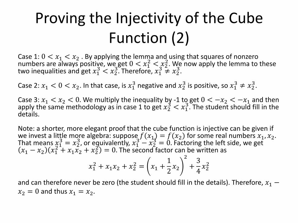
Proving the Injectivity of the Cube Function (2)

Case 1: 0 < 𝑥1 < 𝑥2 . By applying the lemma and using that squares of nonzero numbers are always positive, we get 0 < 𝑥1

2 < 𝑥22. We now apply the lemma to these

two inequalities and get 𝑥13 < 𝑥2

3. Therefore, 𝑥13 ≠ 𝑥2

3.

Case 2: 𝑥1 < 0 < 𝑥2. In that case, is 𝑥13 negative and 𝑥2

3 is positive, so 𝑥13 ≠ 𝑥2

3.

Case 3: 𝑥1 < 𝑥2 < 0. We multiply the inequality by -1 to get 0 < −𝑥2 < −𝑥1 and then apply the same methodology as in case 1 to get 𝑥2

3 < 𝑥13. The student should fill in the

details.

Note: a shorter, more elegant proof that the cube function is injective can be given if we invest a little more algebra: suppose 𝑓(𝑥1) = 𝑓(𝑥2) for some real numbers 𝑥1, 𝑥2.That means 𝑥1

3 = 𝑥23, or equivalently, 𝑥1

3 − 𝑥23 = 0. Factoring the left side, we get

𝑥1 − 𝑥2 𝑥12 + 𝑥1𝑥2 + 𝑥2

2 = 0. The second factor can be written as

𝑥12 + 𝑥1𝑥2 + 𝑥2

2 = 𝑥1 +1

2𝑥2

2

+3

4𝑥22

and can therefore never be zero (the student should fill in the details). Therefore, 𝑥1 −𝑥2 = 0 and thus 𝑥1 = 𝑥2.

A common Misunderstanding of Domain and Range of Inverses

Let us study the following example problem:

If 𝑓: 0,∞ → 0,∞ ; 𝑓 𝑥 = 𝑥, what is the domain of 𝑓−1?

Many students, will immediately get busy going through the algebraic steps they learned for finding an inverse function: write 𝑦 = 𝑥, switch x and y, solve for y again and get 𝑓−1 𝑥 =𝑥2.

Clearly, then, the domain of 𝑓−1 should be all real numbers? Isn’t 𝑥2 defined for all real numbers? It is, but 𝑓−1 𝑥 is only 𝑥2 when x is an output of 𝑓.

The inverse function, by definition, is the function that reverses the action of 𝑓. 𝑓−1 takes an output of 𝑓, and finds the corresponding input of 𝑓.

𝑓 only produces non-negative numbers as outputs. Therefore, 𝑓−1 only takes non-negative numbers as inputs. The domain of 𝑓−1 is therefore 0,∞ .

If you do not find this argument persuasive, consider the graph of 𝑓. It is one branch of a parabola. Therefore, the graph of 𝑓−1 is also only one branch of a parabola. It is the right branch of 𝑦 = 𝑥2.

The domain of 𝑓−1 is always the range of 𝑓, not necessarily the domain implied by the algebraic expression you get when you find 𝑓−1explicitly.

Increasing and Decreasing Functions

Intuitively, a function is strictly increasing if it “always goes up”. It is increasing if it “never goes down”, i.e. “always goes up or is at least constant.”

These concepts requires a rigorous definition that clarifies the meaning of “going up” or “down”:

Let 𝑓: 𝐴 → 𝐵 be a real function, i.e. 𝐴, 𝐵 ⊆ ℝ. Then 𝑓 is called

increasing iff ∀𝑥, 𝑦 ∈ 𝐴 𝑥 < 𝑦 → 𝑓 𝑥 ≤ 𝑓 𝑦 ,

strictly increasing iff ∀𝑥, 𝑦 ∈ 𝐴 𝑥 < 𝑦 → 𝑓 𝑥 < 𝑓 𝑦 ,

decreasing iff ∀𝑥, 𝑦 ∈ 𝐴 𝑥 < 𝑦 → 𝑓 𝑥 ≥ 𝑓 𝑦 ,

strictly decreasing iff ∀𝑥, 𝑦 ∈ 𝐴 𝑥 < 𝑦 → 𝑓 𝑥 > 𝑓 𝑦 .

Note that x and y both represent inputs of 𝑓.

Observe the universal quantifier in the definition - for a function to qualify for any of those four properties, 𝑥 < 𝑦 must always guarantee that 𝑓 𝑥 and 𝑓 𝑦 are in the indicated relationship. 𝑓:ℝ → ℝ; 𝑓 𝑥 = 𝑥2 is not both strictly increasing and decreasing, it is neither. The next slide expands on this point.

A Big Misunderstanding of the Strictly Increasing and Decreasing Properties

Consider the sine function.Some think that it is both strictly increasing and strictlydecreasing, when it is actually neither. They ignore the quantifiers in the definition.

For a function to be strictly increasing, 𝑥 < 𝑦 must ALWAYS guarantee 𝑓 𝑥 < 𝑓 𝑦 , and that is not the case for the sine function, because for some 𝑥 < 𝑦, we have 𝑓 𝑥 ≥ 𝑓 𝑦 (for example, if 𝑥 = 𝜋 and 𝑦 = 3𝜋/2).

Likewise, sine is not strictly decreasing, because for some 𝑥 < 𝑦, we have 𝑓 𝑥 ≤𝑓 𝑦 (for example, if 𝑥 = 0 and 𝑦 = 𝜋/2).

There is only one special condition under which a function can simultaneously be strictly increasing and strictly decreasing. Try to discover it yourself.

Increasing Functions and InequalitiesThe algebraic importance of increasing functions lies in the fact that they preserve non-strict inequalities. More precisely, if you know 𝑎 ≤ 𝑏, and 𝑎, 𝑏 are both in the domain of the increasing function 𝑓, then 𝑓(𝑎) ≤ 𝑓(𝑏) must also be true.

Strictly increasing functions preserve both non-strict and strict inequalities. If 𝑎 ≤ 𝑏, and 𝑎, 𝑏 are both in the domain of the strictly increasing function 𝑓, then 𝑓(𝑎) ≤ 𝑓(𝑏). If 𝑎 <𝑏, then 𝑓 𝑎 < 𝑓(𝑏).

These conclusions may be incorrect if 𝑓 is not (strictly) increasing. Examples:

𝑓:ℝ → ℝ; 𝑓 𝑥 = 𝑒𝑥 is strictly increasing. Thus, 10 < 11 tells us that 𝑒10 < 𝑒11.

𝑓:ℝ → ℝ; 𝑓 𝑥 = 𝑥2 is not strictly increasing. Therefore, even though -5 < 2 is true, the inequality could become false when we square both sides. In fact, 25 is not less than 4.

𝑓: [0,∞) → ℝ; 𝑓 𝑥 = 𝑥2 is strictly increasing. Thus, knowing 101 < 102, we can also be certain that 1012 < 1022.

This is why you must never square both sides of an inequality without careful deliberation. If you know for certain that neither side can be negative, then you can square both sides.

Decreasing Functions and Inequalities

Decreasing functions do not preserve inequalities, but they turn them around in a predictable way.

If 𝑎 ≤ 𝑏, and 𝑎, 𝑏 are both in the domain of the decreasing function 𝑓, then 𝑓 𝑎 ≥ 𝑓 𝑏 .

If 𝑎 < 𝑏, and 𝑎, 𝑏 are both in the domain of the strictly decreasing function 𝑓, then 𝑓 𝑎 > 𝑓 𝑏 . Example:

𝑓: (0,∞) → ℝ; 𝑓 𝑥 = 1/𝑥 is strictly decreasing. Thus, 3 < 5 implies 1/3 > 1/5.

When a function is neither increasing nor decreasing, it does not interact with inequalities in always the same way. For example, 𝑓:ℝ − {0} →ℝ; 𝑓 𝑥 = 1/𝑥 is not decreasing or increasing. It preserves some inequalities and turns around others: -3 < 5 and -1/3 < 1/5 (same relationship) but 3 < 5 and 1/3 > 1/5 (opposite relationship).

Do not take the reciprocal of an inequality without careful deliberation.

The Calculus Connection (1)

Calculus provides non-elementary shortcuts by which we can prove certain properties of differentiable functions: suppose f is a differentiable function defined on an interval. Then if for all 𝑥 in the interval• 𝑓′ 𝑥 ≠ 0, then f is 1-1. • 𝑓′ 𝑥 > 0, then f is strictly increasing. • 𝑓′ 𝑥 ≥ 0, then f is (at least) increasing. (It could still be strictly increasing, as

the example 𝑓 𝑥 = 𝑥3 shows.)

The Mean Value Theorem of Differentiation is the means by which these relationships can be proved: suppose 𝑓 is defined and continuous on the interval 𝑎, 𝑏 , and further suppose that 𝑓 is differentiable at all points strictly between 𝑎 and 𝑏. Then there exists a number 𝑐, strictly between 𝑎 and 𝑏, such that

𝑓 𝑏 − 𝑓 𝑎

𝑏 − 𝑎= 𝑓′ 𝑐 .

The interested student should try to prove the relationships above using the MVT.

The Calculus Connection (2)

To prove that a differentiable function f is onto, the range of f can be determined by using the techniques of calculus to find absolute extrema, or to determine that they don’t exist, and by employing the Intermediate Value Theorem for continuous functions.

Intermediate Value Theorem: suppose 𝑓: 𝑎, 𝑏 →ℝ is continuous. Then any real number between 𝑓(𝑎) and 𝑓(𝑏) occurs as an output of 𝑓.

The Calculus Connection (3)

We will illustrate these techniques by proving that the function 𝑓:ℝ → 0,∞ ; 𝑓 𝑥 = 𝑒𝑥 is bijective. That function is non-elementary - the correct technical term is transcendental, meaning that 𝑒𝑥 cannot be expressed in terms of finitely many elementary algebraic operations. The rigorous calculus definitions all involve limits:

𝑒𝑥 = lim𝑛→∞

1 +𝑥

𝑛

𝑛

=

𝑛=0

∞𝑥𝑛

𝑛!

Since the definition of 𝑒𝑥 involves calculus, any rigorous proof that 𝑓 is bijective must involve calculus.

The Calculus Connection (4)

Proof that 𝑓 is injective: 𝑓 is differentiable, and 𝑓′ 𝑥 = 𝑒𝑥 ≠ 0 for all 𝑥 ∈ ℝ. Now suppose that 𝑥1, 𝑥2 are distinct real numbers. We can assume without loss of generality that 𝑥1 < 𝑥2 (otherwise, we just switch the roles of 𝑥1 and 𝑥2.)

The Mean Value Theorem of differentiation implies that there exists a 𝑐 with

𝑥1 < 𝑐 < 𝑥2 and 𝑓 𝑥2 −𝑓 𝑥1

𝑥2−𝑥1= 𝑓′(𝑐). Since 𝑓′ 𝑐 ≠ 0, we conclude that

𝑓 𝑥2 − 𝑓 𝑥1 ≠ 0, or equivalently, 𝑓 𝑥2 ≠ 𝑓 𝑥1 .

We have shown that 𝑓 𝑥2 ≠ 𝑓 𝑥1 whenever 𝑥1 ≠ 𝑥2. That is the contrapositive definition of injectivity of 𝑓. [Observe that we assumed without proof the non-elementary fact that 𝑒𝑥 ≠ 0 for all 𝑥 ∈ ℝ. This can be proved from either of the two definitions of 𝑒𝑥 using limit laws.]

[We essentially just gave the general proof that if the derivative of a differentiable function on an interval is nonzero, then the function is 1-1.]

The Calculus Connection (5)

Proof that 𝑓 is surjective: let 𝑦 be an arbitrary positive number. Since lim𝑥→∞

𝑒𝑥 = ∞, by definition of what that limit means (𝑒𝑥 will eventually

get larger than any given positive number if we search sufficiently far to the right), we can find a real number 𝑏 so that 𝑒𝑏 > 𝑦.

Since lim𝑥→−∞

𝑒𝑥 = 0, by definition of what that limit means (𝑒𝑥 will

eventually get smaller than any given positive number if we search sufficiently far to the left), we can find a real number 𝑎 so that 𝑒𝑎 < 𝑦.

Therefore, since 𝑒𝑎 < 𝑦 < 𝑒𝑏 , application of the intermediate value theorem to 𝑓 on the interval [𝑎, 𝑏] tells us that 𝑦 is an output of 𝑓, i.e. there exists some 𝑥 between 𝑎 and 𝑏 with 𝑓 𝑥 = 𝑦.

Observe that our argument used not only the intermediate value theorem, but relied heavily on the concept of limit and its exact definition.

Composition

If 𝑔: 𝐴 → 𝐵 and 𝑓: 𝐵 → 𝐶 are functions, then the function 𝑓 ∘ 𝑔: 𝐴 → 𝐶 defined by 𝑓 ∘ 𝑔 𝑥 = 𝑓(𝑔 𝑥 ) for all 𝑥 ∈ 𝐴 is called the composition of 𝑓 with 𝑔. The symbol 𝑓 ∘ 𝑔 is read as “𝑓 composed with 𝑔“.

It is an important theorem that if 𝑔: 𝐴 → 𝐵 and 𝑓: 𝐵 → 𝐶are both bijective, then so is 𝑓 ∘ 𝑔.

[Interestingly, 𝑓 ∘ 𝑔 may be bijective even when 𝑓 and 𝑔are not bijective. Bijectivity of 𝑓, 𝑔 is only a sufficient condition for 𝑓 ∘ 𝑔 to be bijective, not a necessary one.]

We will prove the theorem in two parts.

A composition of 1-1 functions is 1-1

Suppose that 𝑔: 𝐴 → 𝐵 and 𝑓: 𝐵 → 𝐶 are both 1-1. We will show that 𝑓 ∘ 𝑔 is 1-1 as well.

Proof: Suppose 𝑓 ∘ 𝑔 𝑥1 = 𝑓 ∘ 𝑔 𝑥2 for some 𝑥1 and 𝑥2 in 𝐴. By definition of composition, that means

𝑓(𝑔 𝑥1 ) = 𝑓(𝑔 𝑥2 )

Since 𝑓 is 1-1, we conclude that 𝑔 𝑥1 = 𝑔(𝑥2).

Since 𝑔 is 1-1, we conclude that 𝑥1 = 𝑥2.

A composition of onto functions is onto

Suppose that 𝑔: 𝐴 → 𝐵 and 𝑓: 𝐵 → 𝐶 are both onto. We will show that 𝑓 ∘ 𝑔 is onto as well.

Proof: Suppose 𝑧 ∈ 𝐶. Since 𝑓 is onto, there is 𝑦 ∈ 𝐵 with 𝑓 𝑦 = 𝑧. Since 𝑔 is onto, there is 𝑥 ∈ 𝐴 with 𝑔 𝑥 = 𝑦.

By definition of composition, that means

(𝑓 ∘ 𝑔)(𝑥) = 𝑓 𝑔 𝑥 = 𝑓 𝑦 = 𝑧

We have therefore shown that for each 𝑧 ∈ 𝐶, there is 𝑥 ∈ 𝐴such that (𝑓 ∘ 𝑔)(𝑥) = 𝑧. Therefore, we have shown that 𝑓 ∘𝑔 is onto.

Preimage and Image (I)

Inspired by the property 𝑓 𝑓−1 𝑦 = 𝑦 for all 𝑦 ∈𝐵 and 𝑓−1 𝑓 𝑥 = 𝑥 for all 𝑥 ∈ 𝐴 for invertible functions, we ask whether the image and preimage operators satisfy the corresponding relationship:

If 𝑋 ⊆ 𝐴, is 𝑓−1 𝑓 𝑋 equal to 𝑋, and if 𝑌 ⊆ 𝐵, is 𝑓 𝑓−1 𝑌 equal to 𝑌? The answer is generally no. Understanding the reason teaches us a deeper understanding of 1-1 and onto function. On the next slide, we will investigate the problem with an example first.

Preimage and Image (II)

Let 𝑓:ℝ → ℝ; 𝑓 𝑥 = 𝑥2 and 𝑋 = 0,2 .

Then 𝑓 0,2 = [0,4]. Now we see what is going to happen when we apply the preimage. The interval [0,4] is the output of the interval 0,2 , but it is also the output of the interval [−2,0]. The preimage collects all inputs that lead to the specified set of outputs. The function 𝑓 is not 1-1, and in fact every output except zero comes from two different inputs. Therefore, the preimage is going to contain more than the inputs we started with: 𝑓−1(𝑓 0,2 ) = [−2,2].

We therefore arrive at the following hypothesis: for a general function 𝑓, 𝑋 ⊆ 𝑓−1 𝑓 𝑋 , with set equality if 𝑓 is 1-1.

Preimage and Image (III)

We will prove the theorem that we just came up with in two parts.

Let 𝑓: 𝐴 → 𝐵 be a function and 𝑋 ⊆ 𝐴. Then

a. 𝑋 ⊆ 𝑓−1 𝑓 𝑋 .

b. If 𝑓 is 1-1, then 𝑓−1 𝑓 𝑋 ⊆ 𝑋.

Proof:

a. Suppose 𝑡 ∈ 𝑋. By definition of image, 𝑓 𝑡 ∈ 𝑓(𝑋). By definition of preimage, 𝑓−1 𝑓(𝑋) = 𝑥 ∈ 𝑋 𝑓(𝑥) ∈ 𝑓(𝑋) . Since 𝑡 is one of those members of 𝑋 for which the output is in 𝑓 𝑋 , we conclude 𝑡 ∈ 𝑓−1 𝑓(𝑋) .

a. Suppose 𝑡 ∈ 𝑓−1 𝑓 𝑋 . By definition of preimage, that means 𝑓 𝑡 ∈ 𝑓 𝑋 . Since by definition of image, 𝑓 𝑋 is the set of all 𝑓 𝑥 where 𝑥 ∈ 𝑋,we conclude that 𝑓 𝑡 = 𝑓(𝑥) for some 𝑥 ∈ 𝑋. Since 𝑓 is 1-1, 𝑡 = 𝑥, and since 𝑥 ∈ 𝑋, 𝑡 ∈ 𝑋.

A corollary of the this theorem is that if 𝑓: 𝐴 → 𝐵 is a 1-1 function, 𝑋 = 𝑓−1 𝑓 𝑋 .

Preimage and Image (IV)

Let us now investigate the relationship between the two sets 𝑓 𝑓−1 𝑌 and 𝑌 if 𝑌 ⊆ 𝐵 using the square function 𝑓 again. Let 𝑌 =−1,0 . Then 𝑓−1 𝑌 = {0}.

We can already see what prevents 𝑓 𝑓−1 𝑌 and 𝑌 from being equal: not every element of 𝑌 is an output of the function. This is possible because 𝑓 is not onto. Those real numbers that are not in the range of 𝑓 are going to be missing from 𝑓 𝑓−1 𝑌 . Indeed, they will be the only ones missing:

𝑓 𝑓−1 𝑌 = 𝑌 ∩ range 𝑓

For an onto function 𝑓, 𝑓 𝑓−1 𝑌 = 𝑌. To prove these equalities is left as a student exercise.

Application to the Power Set

We conclude this presentation with an important theorem: there can be no onto function from a set to its power set.

We learned previously that the cardinality of the power set of a finite set 𝑆 is given by the equation 𝒫 𝑆 = 2 𝑆 . This means that the cardinality of the power set of 𝑆 is larger than the cardinality of 𝑆, usually vastly larger. It follows, that you could not possibly have a function 𝑓 from 𝑆 onto 𝒫 𝑆because there are too many elements in 𝒫 𝑆 . The range of 𝑓can have at most as many elements as 𝑆 itself.

It is interesting that this theorem remains true if 𝑆 is infinite. The proof, however, requires more sophistication. The heart of the proof lies in an idea known as Russell’s Paradox.

Russell’s Paradox

We shall not make a precise mathematical statement of Russell’s Paradox but merely discuss the following popular form:

Suppose there is a village with just one barber who is a man. Every man of the village either shaves himself, or lets the barber shave him. Therefore, the barber is the man who shaves every man who does not shave himself. Then does the barber shave himself?

The question is a paradox, because either possible answer leads to a contradiction. If the barber shaves himself, then he is one of the men who he is not shaving. If the barber does not shave himself, then he must be shaving himself.

We will construct a version of this paradox to derive a contradiction from the assumption that there is a function from 𝑆 onto 𝒫 𝑆 for some set 𝑆.

Proof of the Statement

Suppose 𝑆 is a set and 𝑓 is a function from 𝑆 onto 𝒫 𝑆 .Observe that this 𝑓 maps every element of 𝑆 to a subset of 𝑆. For each element 𝑠 ∈ 𝑆, there are only two possibilities: 𝑠 ∈ 𝑓(𝑠) or 𝑠 ∉ 𝑓(𝑠).To get a contradiction, we now define the subset 𝑈 ⊆ 𝑆 as follows: 𝑈 is the set of all elements that are not in their own 𝑓 -associated subset. (𝑈 plays the role of the barber):

𝑈 = {𝑥 ∈ 𝑆|𝑥 ∉ 𝑓(𝑥)}

Since 𝑓 is onto, 𝑈 must be the image of some element 𝑢 ∈ 𝑆: 𝑓 𝑢 = 𝑈. We now ask: is 𝑢 ∈ 𝑈? The answer can only be yes or no, and either way, we have a contradiction.

Case 1: 𝑢 ∈ 𝑈. Then by definition of 𝑈, 𝑢 ∉ 𝑓 𝑢 = 𝑈.Case 2: 𝑢 ∉ 𝑈. Then by definition of 𝑈, 𝑢 ∈ 𝑓 𝑢 = 𝑈.

This proves: if 𝑆 is a set, there can be no function from 𝑆 onto 𝒫 𝑆 .