functions

Lecture #3

Functions

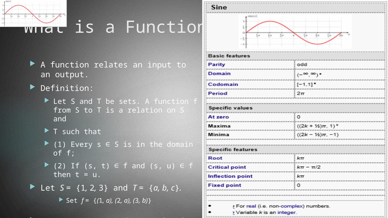
What is a Function?

A function relates an input to an output.

Definition: Let S and T be sets. A function f from S

to T is a relation on S and

T such that

(1) Every s ∈ S is in the domain of f;

(2) If (s, t) ∈ f and (s, u) ∈ f then t = u.

Let S = {1, 2, 3} and T = {a, b, c}. Set f = {(1, a), (2, a), (3, b)}

Let S = {1, 2, 3} and T = {a, b, c, d, e}. Set f = {(1, b), (2, a), (3, c), (4, a), (5,

b)}

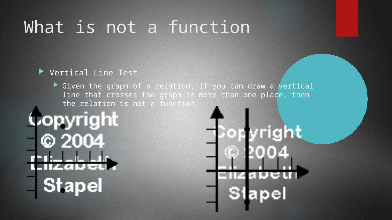
What is not a function

Vertical Line Test Given the graph of a relation, if you can draw a vertical line that

crosses the graph in more than one place, then the relation is not a function.

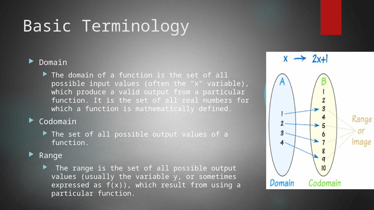
Basic Terminology

Domain The domain of a function is the set of all possible input

values (often the "x" variable), which produce a valid output from a particular function. It is the set of all real numbers for which a function is mathematically defined.

Codomain The set of all possible output values of a function.

Range The range is the set of all possible output values (usually

the variable y, or sometimes expressed as f(x)), which result from using a particular function.

Symbolic Notation

let f denote a function from A into B. Then we write f: A → B

Which is read: “f is a function from A into B,”

“f takes (or maps) A into B.”

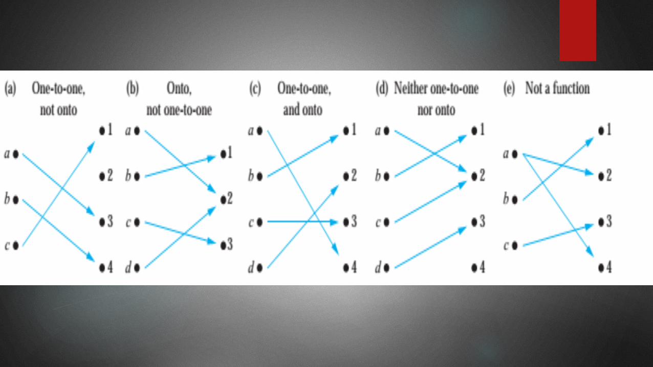
Types of Functions

One-to-One Functions

Onto Functions

Inverse Functions

One-to-One Function

A function f is said to be one-to-one, or an injunction, if and only if f(a) = f(b) implies that a =

b for all a and b in the domain of f.

A function is said to be injective if it is one-to-one.

If different elements in the domain A have distinct images.

A function for which every element of the range of the function corresponds to exactly one element of the domain.

Onto Function

A function f: A → B is said to be an onto function if each element of B is the image of some element of A.

In other words, f: A → B is onto if the image of f is the entire codomain, i.e., if f (A) = B. In such a case we say that f is a function from A onto B or that f maps A onto B.

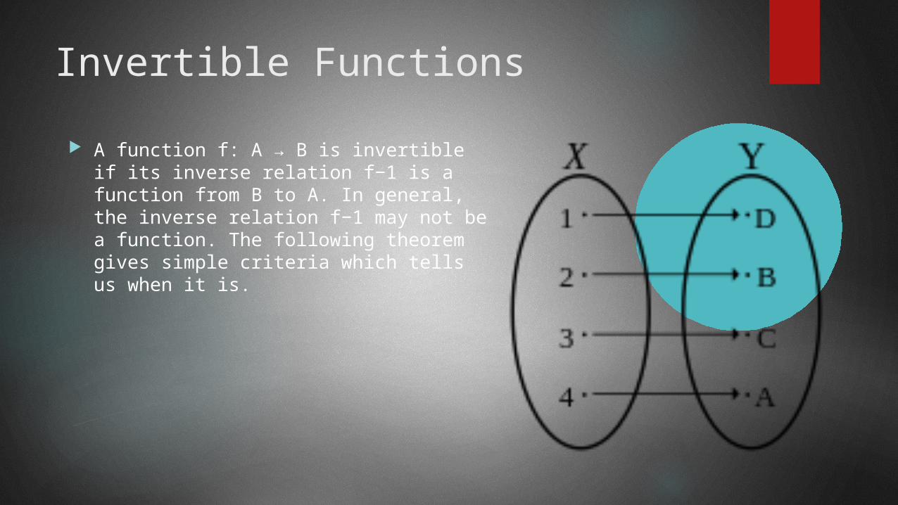
Invertible Functions

A function f: A → B is invertible if its inverse relation f−1 is a function from B to A. In general, the inverse relation f−1 may not be a function. The following theorem gives simple criteria which tells us when it is.

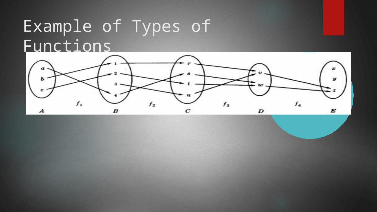
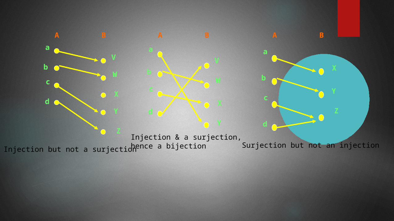
Example of Types of Functions

A B

a

b

c

dX

Y

Z

W

V

Injection but not a surjection

A B

a

b

c

dX

Y

W

V

Injection & a surjection, hence a bijection

A B

a

b

c

d

X

Y

Z

Surjection but not an injection

MATHEMATICAL FUNCTIONS, EXPONENTIAL AND LOGARITHMIC FUNCTIONS

Floor and Ceiling Functions Let x be any real number. Then x lies between two integers called

the floor and the ceiling of x. Specifically,

⌊x⌋ , called the floor of x, denotes the greatest integer that does not exceed x.

⌈x⌉ , called the ceiling of x, denotes the least integer that is not less than x.

If x is itself an integer, then ⌊x⌋ = ⌈x ; otherwise ⌊x⌋ + 1 = ⌈x⌉ .

MATHEMATICAL FUNCTIONS, EXPONENTIAL AND LOGARITHMIC FUNCTIONS For example,

⌊3.14⌋ = 3

⌊√5⌋ = 2

⌊−8.5⌋ = −9

⌊7⌋ = 7

⌊−4⌋ = −4

⌈3.14⌉ = 4

⌈√5⌉ = 3

⌈−8.5⌉ = −8

⌈7⌉ = 7

⌈−4⌉ = −4

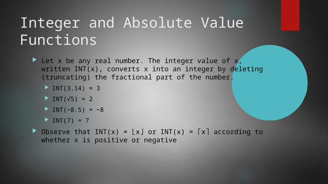
Integer and Absolute Value Functions

Let x be any real number. The integer value of x, written INT(x), converts x into an integer by deleting (truncating) the fractional part of the number. INT(3.14) = 3

INT(√5) = 2

INT(−8.5) = −8

INT(7) = 7

Observe that INT(x) = ⌊x⌋ or INT(x) = ⌈x⌉ according to whether x is positive or negative

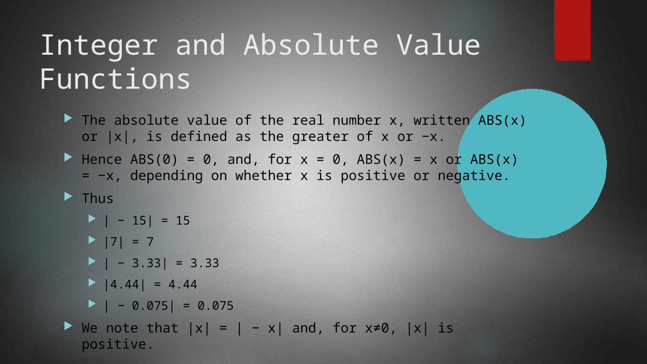
Integer and Absolute Value Functions

The absolute value of the real number x, written ABS(x) or |x|, is defined as the greater of x or −x.

Hence ABS(0) = 0, and, for x = 0, ABS(x) = x or ABS(x) = −x, depending on whether x is positive or negative.

Thus | − 15| = 15

|7| = 7

| − 3.33| = 3.33

|4.44| = 4.44

| − 0.075| = 0.075

We note that |x| = | − x| and, for x≠0, |x| is positive.

Recursively Defined Functions

A function is said to be recursively defined if the function definition refers to itself.

In order for the definition not to be circular, the function definition must have the following two properties:

Base case that tells us directly what the answer is.

In factorial, the base case is factorial(0)=1, this directly tells us the answer; There is a recursive case that defines the answer in terms of the answer to

some other, related problem.

The recursive case is factorial(n) = n * factorial(n-1). This does not directly tell us the answer, but tells how to construct the answer for factorial(n) on the basis of the answer to the related problem, factorial(n-1).

Algorithms and COMPLEXITY OF ALGORITHMS

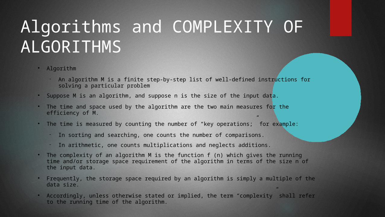
Algorithm

An algorithm M is a finite step-by-step list of well-defined instructions for solving a particular problem

Suppose M is an algorithm, and suppose n is the size of the input data.

The time and space used by the algorithm are the two main measures for the efficiency of M.

The time is measured by counting the number of “key operations;” for example:

In sorting and searching, one counts the number of comparisons.

In arithmetic, one counts multiplications and neglects additions.

The complexity of an algorithm M is the function f (n) which gives the running time and/or storage space requirement of the algorithm in terms of the size n of the input data.

Frequently, the storage space required by an algorithm is simply a multiple of the data size.

Accordingly, unless otherwise stated or implied, the term “complexity” shall refer to the running time of the algorithm.


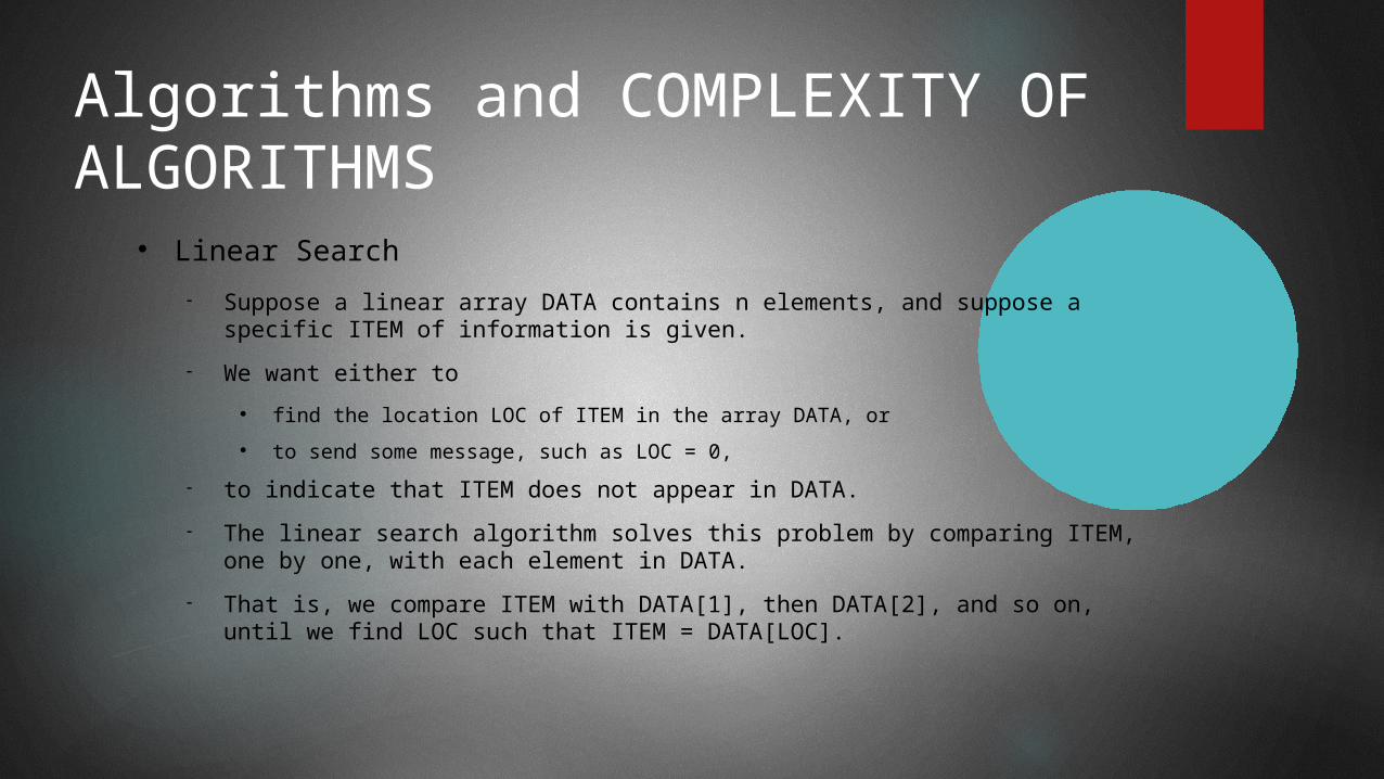
Linear Search

Suppose a linear array DATA contains n elements, and suppose a specific ITEM of information is given.

We want either to

find the location LOC of ITEM in the array DATA, or

to send some message, such as LOC = 0,

to indicate that ITEM does not appear in DATA.

The linear search algorithm solves this problem by comparing ITEM, one by one, with each element in DATA.

That is, we compare ITEM with DATA[1], then DATA[2], and so on, until we find LOC such that ITEM = DATA[LOC].


Linear Search

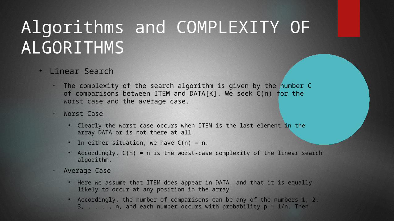
The complexity of the search algorithm is given by the number C of comparisons between ITEM and DATA[K]. We seek C(n) for the worst case and the average case.

Worst Case

Clearly the worst case occurs when ITEM is the last element in the array DATA or is not there at all.

In either situation, we have C(n) = n.

Accordingly, C(n) = n is the worst-case complexity of the linear search algorithm.

Average Case

Here we assume that ITEM does appear in DATA, and that it is equally likely to occur at any position in the array.

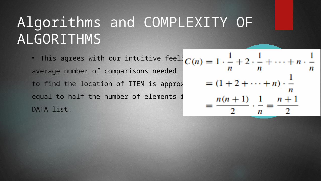
Accordingly, the number of comparisons can be any of the numbers 1, 2, 3, . . . , n, and each number occurs with probability p = 1/n. Then


This agrees with our intuitive feeling that the

average number of comparisons needed

to find the location of ITEM is approximately

equal to half the number of elements in the

DATA list.

Documents

functions