Functional, size and taxonomic diversityof fish along a depth gradient in thedeep sea

Beth L. Mindel1, Francis C. Neat2, Clive N. Trueman3, Thomas J. Webb1

and Julia L. Blanchard4

1 Department of Animal and Plant Sciences, University of Sheffield, Sheffield, United Kingdom2 Marine Scotland, The Scottish Government, Aberdeen, United Kingdom3 Ocean and Earth Science, University of Southampton, Southampton, United Kingdom4 Institute for Marine and Antarctic Studies, University of Tasmania, Hobart, Australia

ABSTRACTBiodiversity is well studied in ecology and the concept has been developed to

include traits of species, rather than solely taxonomy, to better reflect the functional

diversity of a system. The deep sea provides a natural environmental gradient within

which to study changes in different diversity metrics, but traits of deep-sea fish

are not widely known, hampering the application of functional diversity to this

globally important system. We used morphological traits to determine the

functional richness and functional divergence of demersal fish assemblages along the

continental slope in the Northeast Atlantic, at depths of 300–2,000 m. We compared

these metrics to size diversity based on individual body size and species richness.

Functional richness and size diversity showed similar patterns, with the highest

diversity at intermediate depths; functional divergence showed the opposite pattern,

with the highest values at the shallowest and deepest parts of the study site. Species

richness increased with depth. The functional implications of these patterns were

deduced by examining depth-related changes in morphological traits and the

dominance of feeding guilds as illustrated by stable isotope analyses. The patterns

in diversity and the variation in certain morphological traits can potentially be

explained by changes in the relative dominance of pelagic and benthic feeding

guilds. All measures of diversity examined here suggest that the deep areas of the

continental slope may be equally or more diverse than assemblages just beyond the

continental shelf.

Subjects Aquaculture, Fisheries and Fish Science, Biodiversity, Ecology, Marine Biology

Keywords Bathymetry, Deep scattering layer, Environmental gradient, Morphometrics, Rockall

Trough, Trait-based approach, Demersal fish, Continental slope, Biodiversity, Functional role

INTRODUCTIONUnderstanding biotic responses to environmental change remains a major challenge in

ecology. Increasingly, approaches based on quantifying the functional traits of species are

seen as a useful way to meet this challenge (e.g. Harfoot et al., 2014; Violle et al., 2014;

Pawar, Woodward & Dell, 2015). Over the last decade, trait-based approaches have thus

become central to ecology in both terrestrial and marine systems (McGill et al., 2006;

Bremner, 2008; Litchman et al., 2010; Webb et al., 2010; Tyler et al., 2012; Mouillot et al.,

How to cite this articleMindel et al. (2016), Functional, size and taxonomic diversity of fish along a depth gradient in the deep sea. PeerJ

4:e2387; DOI 10.7717/peerj.2387

Submitted 23 June 2015Accepted 31 July 2016Published 15 September 2016

Corresponding authorBeth L. Mindel,

b.l.mindel@gmail.com

Academic editorMarıa Angeles Esteban

Additional Information andDeclarations can be found onpage 19

DOI 10.7717/peerj.2387

Copyright2016 Mindel et al.

Distributed underCreative Commons CC-BY 4.0

2013). Using traits, rather than taxonomy, to describe communities confers several

benefits, such as being more widely applicable to other ecosystems that may share

function even with no taxonomic overlap, reducing the number of variables from

hundreds of species down to only a few traits, and having a clearer connection to the

function and properties of the system than do taxonomic lists (Bremner, 2008; Enquist

et al., 2015; Schmitz et al., 2015). However, the extent to which we can predict the response

of ecosystems to environmental change based on the traits of species remains a

fundamental question in ecology (Sutherland et al., 2013), and more studies of how

different dimensions of diversity vary across environmental gradients are needed.

A trait-based approach that has often been applied to marine systems, including the

deep sea, uses size-based metrics (e.g. Blanchard et al., 2005; Collins et al., 2005; Piet &

Jennings, 2005;Mindel et al., 2016). Body size is important in the oceans because fish grow

several orders of magnitude over the course of their lives, and size, rather than species

identity, often determines what prey is consumed (Cohen et al., 1993; Scharf, Juanes &

Rountree, 2000; Jennings et al., 2001). Body size can be used to calculate a distinct measure

of diversity, based solely on the range of individual sizes present in an assemblage,

irrespective of species identity (e.g. Ye et al., 2013; Rudolf et al., 2014; Quintana et al.,

2015). The diversity of individual sizes present could give more information about

the range of size-based niches a fish community is occupying than does a mean or a

maximum size. Leinster & Cobbold (2012) proposed a measure of diversity based on

Hill numbers (Hill, 1973) that allows traditional measures of diversity based on richness

and evenness to be adjusted to account for the relative similarity of the biological units of

assessment. Similarity can be based on any trait, and although typically the biological

units will be species, the method can be generalised to any biologically meaningful group,

including size classes.

Traits other than body size also impact assemblage function. For example, gape size

can be used as a proxy for what prey are consumed (Boubee & Ward, 1997) and tail

measurements can be used to estimate swimming capabilities (Fisher et al., 2005). In the

deep sea, variation in some morphological characteristics has been attributed to the

habitat occupied. For example, species that aggregate at seamounts are deep-bodied to

cope with the strong currents in these areas (Koslow, 1996; Koslow et al., 2000) and

deeper-living species have more elongated body plans to increase swimming efficiency

(Neat & Campbell, 2013). Locomotory capacity also declines with depth, which is likely a

response to decreased light for vision that relaxes the demand for high activity levels

needed to obtain prey or escape predation (Childress, 1995). Age at maturity increases

with depth while fecundity and potential rate of population growth decrease (Drazen &

Haedrich, 2012), ultimately having important implications for the productivity and

resilience of deep-sea populations. Traits are also able to predict where or on what a

species is feeding. Species that vertically migrate through the water column to feed on

pelagic prey have worldwide impacts for carbon storage in the deep sea (Trueman et al.,

2014). Furthermore, scavengers exhibit different traits to non-scavengers due to the

high-energy reward of carrion compared to the low food availability for predators in the

deep (Haedrich & Rowe, 1977; Collins et al., 2005). Large food falls are an important

Mindel et al. (2016), PeerJ, DOI 10.7717/peerj.2387 2/25

resource in the deep sea (Hilario et al., 2015) and scavengers that exploit

this resource must possess traits such as the ability to undergo prolonged starvation,

recognition of carrion odours, and sufficient motility to locate and reach the carcass

(Tamburri & Barry, 1999).

Thus, traits determine what individuals feed on, where they live, and ultimately the

function of deep-sea ecosystems. How communities function is not constant throughout

the deep sea, as it is now known to be a diverse environment (Danovaro, Snelgrove &

Tyler, 2014). The continental slope, which links shallow waters to the abyssal plain,

experiences profound environmental changes due to depth, such as increased pressure

and decreased temperature, light and food availability (Lalli & Parsons, 1993; Kaiser

et al., 2011). These changes mean that assemblage structure varies more on a vertical

gradient than it does horizontally (i.e. spatially; Angel, 1993; Lalli & Parsons, 1993; Kaiser

et al., 2011), but what these structural changes mean in terms of distribution of traits

and function is not yet known.

A popular approach that uses traits as building blocks is functional diversity (Tilman,

2001; Petchey & Gaston, 2002), which aims to quantify differences and similarities in

function and role between species. Higher species richness may not necessarily confer a

more diverse ecosystem if species overlap in the roles they perform (Walker, 1992);

functional diversity aims to address this by quantifying the distinctness of different species

based on biological traits. How traits are partitioned among groups of co-occurring

species is debated. The ‘limiting similarity’ hypothesis predicts that species that occupy

similar niches will not be able to co-exist due to interspecific competition (Macarthur &

Levins, 1967), resulting in high diversity of traits (Mouillot, Dumay & Tomasini, 2007).

The ‘environmental filtering’ hypothesis states that species must adapt in similar ways

to local abiotic conditions, resulting in the co-existence of similar species (Keddy, 1992;

Violle et al., 2007) and hence low trait diversity (Mouillot, Dumay & Tomasini, 2007).

Alternatively, under the neutral hypothesis (Hubbell, 2001; Hubbell, 2005), no species are

at a competitive advantage or disadvantage, so assemblages are formed by stochastic

processes. Along the depth gradient of the continental slope, resource availability declines

and environmental conditions become more extreme (Carney, 2005). It could therefore

be expected that functional diversity will be highest in the shallowest areas where ‘limiting

similarity’ causes species to occupy different niches (Macarthur & Levins, 1967), while in

the deepest areas, the harsh conditions result in ‘environmental filtering’ (Keddy, 1992;

Violle et al., 2007) and hence a reduction in functional diversity.

We use the depth gradient of the continental slope to compare the trait-based

approaches of functional diversity calculated using species-level morphological traits, and

size diversity calculated using individual body size data, to a simple measure of taxonomic

diversity, species richness. We investigate the drivers behind patterns in functional

diversity by examining average morphological trait values across the depth gradient. This

allows us to deduce which traits are contributing most to values of functional diversity

and also to explore how morphological traits relate to the dominance of feeding

guilds. Feeding guilds were established using stable isotope analysis, which reveals the

position of an individual in the food chain from the relative concentrations of light

Mindel et al. (2016), PeerJ, DOI 10.7717/peerj.2387 3/25

and heavy isotopes of nitrogen and carbon in body tissue (e.g. Michener & Schell, 1994),

hence allowing us to class species as either benthic or pelagic feeders. We use this

combination of taxonomic and trait-based approaches to answer for the first time in

deep-sea fish assemblages the following key questions: i) How does functional diversity

based on species-level traits vary along a depth gradient? ii) How do patterns in functional

diversity compare to depth-dependent changes in species richness and the diversity of

individual body sizes? iii) What traits are driving the changes in functional diversity

along a depth gradient, and how do these traits relate to the relative dominance of

feeding guilds?

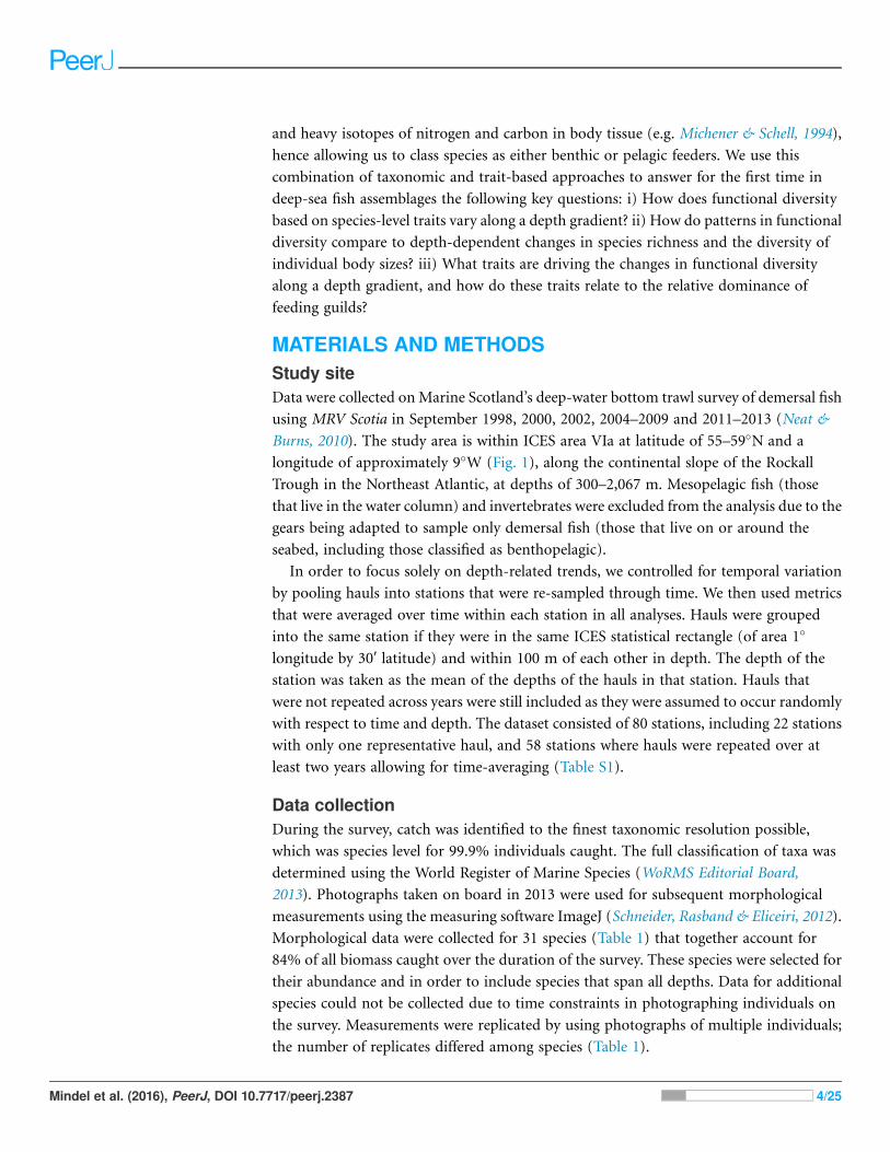
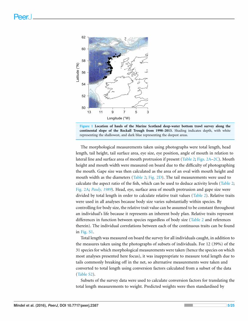
MATERIALS AND METHODSStudy siteData were collected on Marine Scotland’s deep-water bottom trawl survey of demersal fish

using MRV Scotia in September 1998, 2000, 2002, 2004–2009 and 2011–2013 (Neat &

Burns, 2010). The study area is within ICES area VIa at latitude of 55–59�N and a

longitude of approximately 9�W (Fig. 1), along the continental slope of the Rockall

Trough in the Northeast Atlantic, at depths of 300–2,067 m. Mesopelagic fish (those

that live in the water column) and invertebrates were excluded from the analysis due to the

gears being adapted to sample only demersal fish (those that live on or around the

seabed, including those classified as benthopelagic).

In order to focus solely on depth-related trends, we controlled for temporal variation

by pooling hauls into stations that were re-sampled through time. We then used metrics

that were averaged over time within each station in all analyses. Hauls were grouped

into the same station if they were in the same ICES statistical rectangle (of area 1�

longitude by 30′ latitude) and within 100 m of each other in depth. The depth of the

station was taken as the mean of the depths of the hauls in that station. Hauls that

were not repeated across years were still included as they were assumed to occur randomly

with respect to time and depth. The dataset consisted of 80 stations, including 22 stations

with only one representative haul, and 58 stations where hauls were repeated over at

least two years allowing for time-averaging (Table S1).

Data collectionDuring the survey, catch was identified to the finest taxonomic resolution possible,

which was species level for 99.9% individuals caught. The full classification of taxa was

determined using the World Register of Marine Species (WoRMS Editorial Board,

2013). Photographs taken on board in 2013 were used for subsequent morphological

measurements using the measuring software ImageJ (Schneider, Rasband & Eliceiri, 2012).

Morphological data were collected for 31 species (Table 1) that together account for

84% of all biomass caught over the duration of the survey. These species were selected for

their abundance and in order to include species that span all depths. Data for additional

species could not be collected due to time constraints in photographing individuals on

the survey. Measurements were replicated by using photographs of multiple individuals;

the number of replicates differed among species (Table 1).

Mindel et al. (2016), PeerJ, DOI 10.7717/peerj.2387 4/25

The morphological measurements taken using photographs were total length, head

length, tail height, tail surface area, eye size, eye position, angle of mouth in relation to

lateral line and surface area of mouth protrusion if present (Table 2; Figs. 2A–2C). Mouth

height and mouth width were measured on board due to the difficulty of photographing

the mouth. Gape size was then calculated as the area of an oval with mouth height and

mouth width as the diameters (Table 2; Fig. 2D). The tail measurements were used to

calculate the aspect ratio of the fish, which can be used to deduce activity levels (Table 2;

Fig. 2A; Pauly, 1989). Head, eye, surface area of mouth protrusion and gape size were

divided by total length in order to calculate relative trait values (Table 2). Relative traits

were used in all analyses because body size varies substantially within species. By

controlling for body size, the relative trait value can be assumed to be constant throughout

an individual’s life because it represents an inherent body plan. Relative traits represent

differences in function between species regardless of body size (Table 2 and references

therein). The individual correlations between each of the continuous traits can be found

in Fig. S1.

Total length was measured on board the survey for all individuals caught, in addition to

the measures taken using the photographs of subsets of individuals. For 12 (39%) of the

31 species for which morphological measurements were taken (hence the species on which

most analyses presented here focus), it was inappropriate to measure total length due to

tails commonly breaking off in the net, so alternative measurements were taken and

converted to total length using conversion factors calculated from a subset of the data

(Table S2).

Subsets of the survey data were used to calculate conversion factors for translating the

total length measurements to weight. Predicted weights were then standardised by

Longitude (°W)

Latit

ude

(°N

)

50

52

54

56

58

60

62

13 11 9 7 5 3

Figure 1 Location of hauls of the Marine Scotland deep-water bottom trawl survey along the

continental slope of the Rockall Trough from 1998–2013. Shading indicates depth, with white

representing the shallowest, and dark blue representing the deepest areas.

Mindel et al. (2016), PeerJ, DOI 10.7717/peerj.2387 5/25

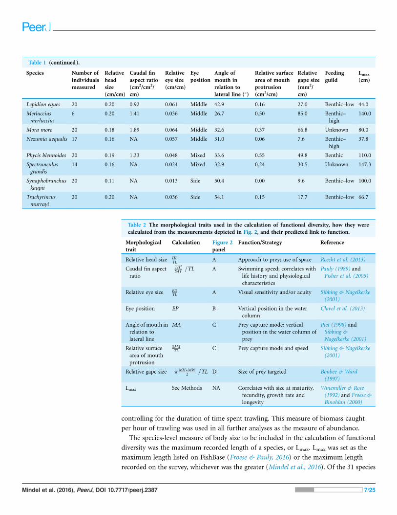
Table 1 Species-level trait data for the 31 species for which morphological measurements were collected. Lmax was downloaded from FishBase

(Froese & Pauly, 2016) or calculated from the survey data (please see Methods for details), feeding guild classification was based on stable isotope

analyses, and all other traits were measured from photos taken on Marine Scotland’s deep-water trawl survey in 2013. Please refer to Fig. 2 and

Table 2 for definitions and calculations of traits.

Species Number of

individuals

measured

Relative

head

size

(cm/cm)

Caudal fin

aspect ratio

(cm2/cm2/

cm)

Relative

eye size

(cm/cm)

Eye

position

Angle of

mouth in

relation to

lateral line (�)

Relative surface

area of mouth

protrusion

(cm2/cm)

Relative

gape size

(mm2/

cm)

Feeding

guild

Lmax

(cm)

Alepocephalus

agassizii

22 0.29 3.11 0.074 Side 25.6 0.34 75.7 Pelagic 123.0

Alepocephalus

bairdii

19 0.21 5.29 0.065 Side 23.3 0.19 43.8 Pelagic 127.4

Antimora rostrata 16 0.21 2.77 0.044 Side 16.5 0.17 58.2 Unknown 87.0

Aphanopus carbo 19 0.19 3.09 0.032 Side 16.9 0.00 55.8 Pelagic–high 129.0

Apristurus

aphyodes

13 0.24 0.38 0.013 Side 9.3 0.00 20.4 Benthic 85.0

Argentina silus 20 0.19 3.53 0.087 Side 26.5 0.13 14.9 Pelagic 81.1

Bathypterois

dubius

18 0.16 3.10 0.010 Side 21.1 0.17 24.8 Unknown 29.0

Bathysaurus ferox 6 0.14 2.19 0.018 Side 28.8 0.00 97.2 Unknown 74.2

Beryx

decadactylus

17 0.24 3.93 0.111 Side 35.1 1.30 93.4 Unknown 100.0

Cataetyx laticeps 10 0.21 NA 0.020 Top 28.2 0.51 101.1 Benthic–

suspension

101.0

Centroscymnus

coelolepis

1 0.15 2.58 0.021 Side NA NA 35.5 Benthic 122.0

Chimaera

monstrosa

19 0.15 NA 0.037 Side 48.3 0.08 7.9 Benthic 150.0

Coelorinchus

caelorhincus

16 0.18 NA 0.045 Side 50.9 0.10 10.2 Benthic–low 48.0

Coelorinchus

labiatus

20 0.26 NA 0.046 Side 57.7 0.12 5.9 Unknown 50.0

Coryphaenoides

guentheri

21 0.17 NA 0.044 Side 35.6 0.06 6.7 Benthic 55.3

Coryphaenoides

mediterraneus

19 0.10 NA 0.023 Side 47.5 0.19 19.8 Benthic–low 105.8

Coryphaenoides

rupestris

29 0.15 NA 0.038 Side 56.0 0.27 25.4 Pelagic 127.7

Halargyreus

johnsonii

20 0.22 2.72 0.061 Side 42.7 0.22 27.9 Unknown 56.0

Halosauropsis

macrochir

11 0.13 NA 0.012 Side 44.7 0.08 15.9 Benthic–

high

90.0

Harriotta

raleighana

9 0.30 NA 0.027 Side NA NA 6.6 Unknown 120.0

Helicolenus

dactylopterus

20 0.31 2.27 0.076 Side 46.5 0.67 76.3 Benthic 47.0

Hoplostethus

atlanticus

15 0.30 3.82 0.067 Side 40.2 0.82 140.8 Benthic 75.0

Hydrolagus affinis 9 0.20 0.49 0.029 Side NA NA 19.3 Unknown 131.6

Mindel et al. (2016), PeerJ, DOI 10.7717/peerj.2387 6/25

controlling for the duration of time spent trawling. This measure of biomass caught

per hour of trawling was used in all further analyses as the measure of abundance.

The species-level measure of body size to be included in the calculation of functional

diversity was the maximum recorded length of a species, or Lmax. Lmax was set as the

maximum length listed on FishBase (Froese & Pauly, 2016) or the maximum length

recorded on the survey, whichever was the greater (Mindel et al., 2016). Of the 31 species

Table 2 The morphological traits used in the calculation of functional diversity, how they were

calculated from the measurements depicted in Fig. 2, and their predicted link to function.

Morphological

trait

Calculation Figure 2

panel

Function/Strategy Reference

Relative head size HLTL

A Approach to prey; use of space Reecht et al. (2013)

Caudal fin aspect

ratio

TH2

SAT

� �=TL A Swimming speed; correlates with

life history and physiological

characteristics

Pauly (1989) and

Fisher et al. (2005)

Relative eye size EDTL

A Visual sensitivity and/or acuity Sibbing & Nagelkerke

(2001)

Eye position EP B Vertical position in the water

column

Clavel et al. (2013)

Angle of mouth in

relation to

lateral line

MA C Prey capture mode; vertical

position in the water column of

prey

Piet (1998) and

Sibbing &

Nagelkerke (2001)

Relative surface

area of mouth

protrusion

SAMTL

C Prey capture mode and speed Sibbing & Nagelkerke

(2001)

Relative gape size �MH�MW2

� �=TL D Size of prey targeted Boubee & Ward

(1997)

Lmax See Methods NA Correlates with size at maturity,

fecundity, growth rate and

longevity

Winemiller & Rose

(1992) and Froese &

Binohlan (2000)

Table 1 (continued).

Species Number of

individuals

measured

Relative

head

size

(cm/cm)

Caudal fin

aspect ratio

(cm2/cm2/

cm)

Relative

eye size

(cm/cm)

Eye

position

Angle of

mouth in

relation to

lateral line (�)

Relative surface

area of mouth

protrusion

(cm2/cm)

Relative

gape size

(mm2/

cm)

Feeding

guild

Lmax

(cm)

Lepidion eques 20 0.20 0.92 0.061 Middle 42.9 0.16 27.0 Benthic–low 44.0

Merluccius

merluccius

6 0.20 1.41 0.036 Middle 26.7 0.50 85.0 Benthic–

high

140.0

Mora moro 20 0.18 1.89 0.064 Middle 32.6 0.37 66.8 Unknown 80.0

Nezumia aequalis 17 0.16 NA 0.057 Middle 31.0 0.06 7.6 Benthic–

high

37.8

Phycis blennoides 20 0.19 1.33 0.048 Mixed 33.6 0.55 49.8 Benthic 110.0

Spectrunculus

grandis

14 0.16 NA 0.024 Mixed 32.9 0.24 30.5 Unknown 147.3

Synaphobranchus

kaupii

20 0.11 NA 0.013 Side 50.4 0.00 9.6 Benthic–low 100.0

Trachyrincus

murrayi

20 0.20 NA 0.036 Side 54.1 0.15 17.7 Benthic–low 66.7

Mindel et al. (2016), PeerJ, DOI 10.7717/peerj.2387 7/25

for which morphological data were available, one (Apristurus aphyodes) did not have an

Lmax listed on FishBase. Therefore, its Lmax was set as that of the largest species of that

genus caught on the survey (Apristurus manis). Standard Lengths on FishBase were

converted to total length using conversion factors calculated from the survey data where

possible (Table S2). If there was no survey-derived conversion factor available (due to total

length being measured on the survey and Standard Length being provided by FishBase)

then the conversion factor listed on FishBase was used. Where both conversion factors

were missing, we used an average conversion factor that was calculated across all species

caught on the survey for which there was a Standard Length conversion available.

Stable isotope data were available for 21 of the species for which morphological

data were collected. The stable isotope analyses are described in Trueman et al. (2014;

data are available at Dryad Digital Respository doi: 10.5061/dryad.n576n). The isotopic

dataset was compared to a meta-dataset of diet studies based on stomach content

analyses (Trueman et al., 2014). Where species were present in both datasets, stable isotope

compositions clearly distinguished between species categorised as feeding on either

benthic (seabed) or pelagic (water column) prey (Trueman et al., 2014). Stable isotope

compositions were subsequently used to assign feeding guild to species and individuals

lacking reliable stomach content data (Trueman et al., 2014). The distinction between

benthic and pelagic feeders was less pronounced in the assemblage at 500 m, as the diets of

Figure 2 How morphological measurements were taken using photographs (panels A, B and C) and

on board the survey (panel D). Morphological traits were calculated from these measurements using

the formulae in Table 2. (A) TL, total length; HL, head length; ED, eye diameter; SAT, surface area of

tail; TH, tail height. (B) EP, eye position. (C) SAM, surface area of mouth protrusion; MA, mouth angle.

(D) MW, mouth width; MH, mouth height.

Mindel et al. (2016), PeerJ, DOI 10.7717/peerj.2387 8/25

the two guilds are similar at this depth. However, species could still be assigned to a

feeding guild based on their relative isotope signatures throughout the rest of their depth

range. Specialised signatures within these two feeding guilds could be established in some

cases: if the smallest individual sampled for that species was in the upper half of stable

isotope space for that category, the species was defined as high trophic level; if the largest

individual sampled was in the lower half of stable isotope space, the species was defined as

low trophic level; fish that feed on benthic suspension feeding prey have a noticeably

enriched isotope signature for a given body size, depth and feeding guild, so were

categorised separately.

Data analysisDiversity was calculated in four ways: 1) functional richness, 2) functional divergence,

3) size diversity, and 4) species richness. The two measures of functional diversity are

described by Villeger, Mason & Mouillot (2008) and were calculated using the R (R Core

Team, 2015) package FD (Laliberte & Shipley, 2011). Functional richness is an estimate

of the degree to which the assemblage fills functional space (Fig. 3A; Villeger, Mason &

Mouillot, 2008) and functional divergence measures how abundance is distributed within

the volume of functional trait space occupied by species (Fig. 3B; Villeger, Mason &

Mouillot, 2008). The traits included in the calculation of functional diversity were relative

head size, aspect ratio of the caudal fin, relative eye size, eye position, angle of mouth

in relation to lateral line, relative surface area of mouth protrusion if present, relative

gape size, and Lmax (Table 2). A species-level mean was calculated from the relative trait

values for all continuous traits (Table 1). Functional richness does not include species

abundances in its calculation; functional divergence includes a weighting of traits by

species abundance, which in this case was biomass caught per hour of trawling. Due

to only having trait data for a maximum of 31 species, functional diversity was only

calculated using those species and their biomasses, and the rarer species were not

considered. As these 31 species accounted for 84% of all biomass caught on the survey

and spanned the entirety of the depth range studied, they were considered to be a good

representation of the study system.

Size diversity was calculated using the generalised measure of diversity proposed by

Leinster & Cobbold (2012). In this index, abundance of biologically meaningful groups

and similarities between them are accounted for. Here the groups were size classes

each of 10 cm in width, and abundance was calculated as the proportional biomass

per hour that each size class accounts for in each station, when only the species for which

morphological data were known were included. The Euclidean distance matrix (d)

between the mid-points of size classes was converted to similarities using the formula

suggested by Leinster & Cobbold (2012):

Similarity ¼ e

log 2ð Þ � dThe final input for the Leinster-Cobbold measure of diversity is the sensitivity

parameter, q, which determines how much emphasis is given to rare species (or in

Mindel et al. (2016), PeerJ, DOI 10.7717/peerj.2387 9/25

this case, size classes; Leinster & Cobbold, 2012). Here a value of q = 1.1 was used in

order to balance the richness (lower q) and evenness (higher q) components of diversity,

and to be comparable to the widely used Shannon index (Shannon, 1948; Leinster &

Cobbold, 2012).

Species richness was calculated using only hauls that were of 120 ± 5 min in duration

in order to control for sampling effort. For this subset of hauls, the number of species

present was averaged across hauls in each station. All species were included in the

calculation of species richness, not just those with morphological data available. This

is because calculating species richness using only the morphological subset would

merely be a count of the number of species for which morphological data were available

and not be meaningful in a diversity context.

The four diversity measures were calculated for each station and then analysed with

respect to the depth of that station with Generalised Additive Models (GAMs) using the

R (R Core Team, 2015) package mgcv (Wood, 2011). A smoother function of depth was

used as the predictor, and the values for the test statistic, significance, R-squared, and

effective degrees of freedom (e.d.f.; the flexibility of the fitted model; Wood, 2006) were

extracted from the model summary.

Abundance-weighted station means were calculated for each continuous

morphological trait included in the functional diversity metric and analysed with respect

to the depth of the station using GAMs. The weighted mean was said to be the mean

value across species, where values were weighted by the biomass caught per hour of

trawling for each species. The mean observed size of individuals, irrespective of species

identity, was also calculated for comparison. This value was not included in the functional

diversity metric because a species-level measure of body size (Lmax) was needed. The

station mean body size was therefore calculated as the average length across individuals

0.0 0.5 1.0 1.5 2.0

0.0

0.5

1.0

1.5

2.0

Trait 1

Trai

t 2

A

0.0 0.5 1.0 1.5 2.0

0.0

0.5

1.0

1.5

2.0

Trait 1

Trai

t 2

B

Figure 3 Toy example using only two traits of the calculation of (A) functional richness and (B)

functional divergence. Each black point represents a species that exhibits trait values indicated by

their positioning within the axes, and the size of the point represents the abundance of that species.

(A) Functional richness is represented by the green shaded area, corresponding to the volume of trait

space occupied by the species. (B) Functional divergence is determined by species abundances, how far

those species are from the centre of gravity as determined by the species traits (illustrated by dashed

lines), and how this distance compares to the mean distance to the centre of gravity (illustrated by the

circle). Figures are adapted from Villeger, Mason & Mouillot (2008).

Mindel et al. (2016), PeerJ, DOI 10.7717/peerj.2387 10/25

in a station, when only individuals of species for which morphological data were

obtained were included, in order to be comparable to the measures of functional and

size diversity. The standard deviation of each continuous trait at each station was also

calculated and analysed with respect to depth using GAMs in order to relate variation

in traits to patterns seen in functional diversity. The Pearson’s product-moment

correlation coefficient was calculated for the relationships between the means and

standard deviations of each of the traits, and each measure of diversity.

The isotopic feeding guild data (Table 1) were interpreted using the percentage of

biomass that each guild accounted for in depth bands of 200 m in width. The percentage

was calculated as a proportion of the biomass accounted for by the species for which

there were morphological data.

All data manipulation and analysis was performed using R version 3.1.2 (R Core

Team, 2015) and figures were produced using the packages ggplot2 (Wickham, 2009),

gridExtra (Auguie, 2016) and marmap (Pante & Simon-Bouhet, 2013).

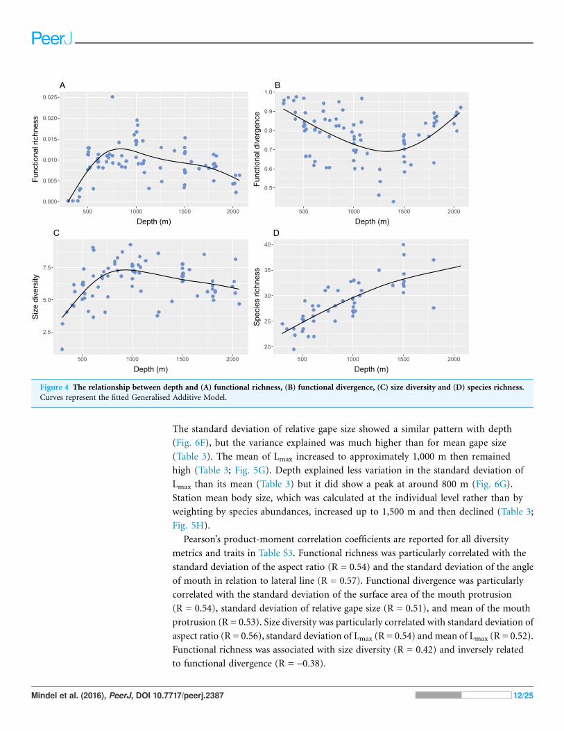
RESULTSFunctional richness was low in the shallowest and deepest depths, and high at around

800 m (Fig. 4A; GAM: F = 14.1, e.d.f. = 3.8, R2 = 0.40, p < 0.001). Functional divergence

was high at both the shallow and deep ends of the depth gradient, with lowest values at

around 1,300 m (Fig. 4B; GAM: F = 10.4, e.d.f. = 2.9, R2 = 0.31, p < 0.001). Size diversity

increased to a peak at roughly 900 m, then declined as depth increased further, but

remained higher in the deepest areas than in the shallowest ones (Fig. 4C; GAM: F = 10.8,

e.d.f. = 3.5, R2 = 0.33, p < 0.001). Species richness increased significantly with depth

(Fig. 4D; GAM: F = 34.2, e.d.f. = 1.9, R2 = 0.61, p < 0.001).

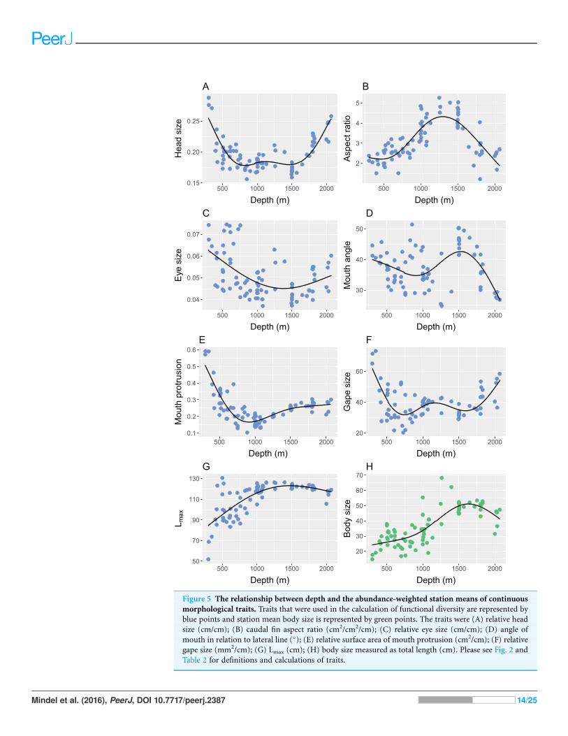
Abundance-weighted station means and the standard deviation of continuous

morphological variables changed with depth and all statistics are reported in Table 3.

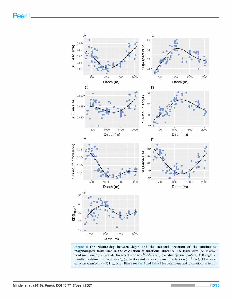
The mean and standard deviation of relative head size exhibited strong relationships

with depth (Table 3), where heads were larger in proportion to body size, and more

varied, in the shallowest and deepest parts of the study site (Figs. 5A and 6A). Mean and

standard deviation of aspect ratio also varied strongly with depth (Table 3), showing

peaks at 1,000–1,500 m (Figs. 5B and 6B). Depth did not explain as much variation in

relative eye size as it did relative head size (Table 3), but there was still a significant

relationship and eye size was largest at the shallowest depths (Fig. 5C). Variation in

eye size was highest at the deepest depths (Fig. 6C). The mean angle of the mouth

in relation to the lateral line varied with depth but the variance explained was low

(Table 3). However, the standard deviation of the mouth angle showed a highly

significant pattern with depth (Table 3), with the highest variation at intermediate

depths (Fig. 6D). The mean and standard deviation of the relative surface area of

the mouth protrusion exhibited strong relationships with depth (Table 3) where

both values were high in the shallows then decreased and remained constant from

1,000–2,000 m (Figs. 5E and 6E). Depth explained an intermediate amount of variation

in mean relative gape size (Table 3), which showed a pattern similar to that of head size,

with the highest values at the shallowest and deepest parts of the study site (Fig. 5F).

Mindel et al. (2016), PeerJ, DOI 10.7717/peerj.2387 11/25

The standard deviation of relative gape size showed a similar pattern with depth

(Fig. 6F), but the variance explained was much higher than for mean gape size

(Table 3). The mean of Lmax increased to approximately 1,000 m then remained

high (Table 3; Fig. 5G). Depth explained less variation in the standard deviation of

Lmax than its mean (Table 3) but it did show a peak at around 800 m (Fig. 6G).

Station mean body size, which was calculated at the individual level rather than by

weighting by species abundances, increased up to 1,500 m and then declined (Table 3;

Fig. 5H).

Pearson’s product-moment correlation coefficients are reported for all diversity

metrics and traits in Table S3. Functional richness was particularly correlated with the

standard deviation of the aspect ratio (R = 0.54) and the standard deviation of the angle

of mouth in relation to lateral line (R = 0.57). Functional divergence was particularly

correlated with the standard deviation of the surface area of the mouth protrusion

(R = 0.54), standard deviation of relative gape size (R = 0.51), and mean of the mouth

protrusion (R = 0.53). Size diversity was particularly correlated with standard deviation of

aspect ratio (R = 0.56), standard deviation of Lmax (R = 0.54) andmean of Lmax (R = 0.52).

Functional richness was associated with size diversity (R = 0.42) and inversely related

to functional divergence (R = -0.38).

0.000

0.005

0.010

0.015

0.020

0.025

500 1000 1500 2000

Depth (m)

Func

tiona

l ric

hnes

s

A

2.5

5.0

7.5

500 1000 1500 2000

Depth (m)

Siz

e di

vers

ity

C

0.5

0.6

0.7

0.8

0.9

1.0

500 1000 1500 2000

Depth (m)

Func

tiona

l div

erge

nce

B

20

25

30

35

40

500 1000 1500 2000

Depth (m)

Spe

cies

rich

ness

D

Figure 4 The relationship between depth and (A) functional richness, (B) functional divergence, (C) size diversity and (D) species richness.

Curves represent the fitted Generalised Additive Model.

Mindel et al. (2016), PeerJ, DOI 10.7717/peerj.2387 12/25

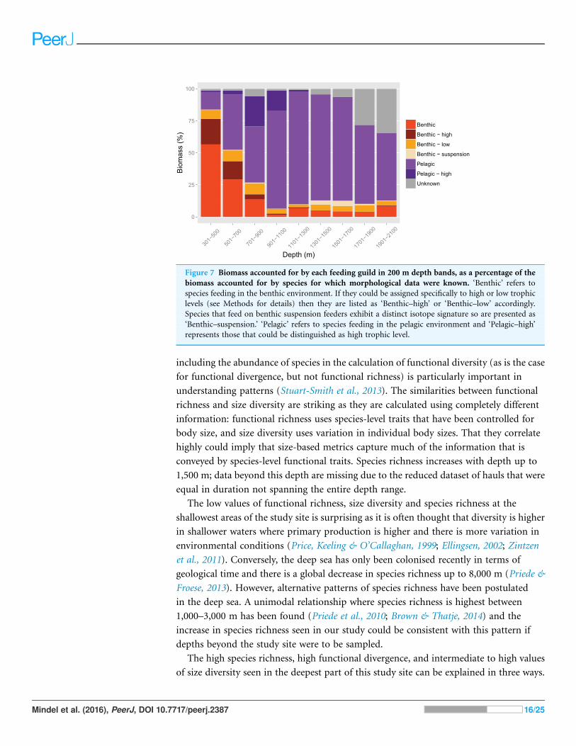
Relative contributions of feeding guilds to total biomass changed with depth (Fig. 7).

Benthic feeders were the largest component of biomass up to 700 m then declined as

depth increased. The benthic feeders that were of particularly high or low trophic

levels followed the same pattern, but those of a high trophic level virtually disappeared

at around 1,100 m. The specialised fish that feed on benthic suspension feeders lived

mainly at 1,300–1,900 m. Generalist pelagic feeders increased with depth and dominated

the biomass from 700 m, then started to decline in dominance at particularly deep

depths. The high trophic level pelagic feeders were abundant only from 500–1,100 m. The

biomass accounted for by species for which isotopic signatures were not known increased

with depth.

DISCUSSIONThe four measures of diversity examined here exhibit different patterns along a depth

gradient, but all show intermediate or high values in the deepest part of the study site

(Fig. 4). At the shallower end of the continental slope, functional richness, size diversity

and species richness indicate low levels of diversity, but functional divergence is high. This

implies that species are widely and unevenly distributed around the small amount of trait-

space occupied (Fig. 3). The deepest areas exhibit similar patterns but functional richness

and size diversity are higher than in the shallowest areas. Functional richness and size

diversity are both highest at around 800–1,000 m in depth where functional divergence is

low, implying that species are evenly distributed around a wide range of trait space. The

conflicting patterns of the two different measures of functional diversity have been found

previously in a global analysis of reef fish communities, and it has been suggested that

Table 3 Statistics extracted from Generalised Additive Models (GAMs) on the relationships between

trait means and trait variances in a station, and the depth of that station.

Trait Calculation F e.d.f. R2 p

Relative head size (cm/cm) Mean 37.6 3.9 0.65 < 0.001

SD 33.6 3.3 0.62 < 0.001

Caudal fin aspect ratio (cm2/cm2/cm) Mean 34.7 3.8 0.63 < 0.001

SD 36.7 3.4 0.64 < 0.001

Relative eye size (cm/cm) Mean 10.5 2.3 0.28 < 0.001

SD 9.4 2.9 0.29 < 0.001

Mouth angle (�) Mean 7.3 3.7 0.28 < 0.001

SD 39.0 3.4 0.65 < 0.001

Relative surface area of mouth protrusion (cm2/cm) Mean 46.6 3.8 0.70 < 0.001

SD 81.4 3.8 0.80 < 0.001

Relative gape size (mm2/cm) Mean 14.9 3.9 0.42 < 0.001

SD 40.1 3.0 0.65 < 0.001

Lmax (cm) Mean 31.8 2.5 0.56 0.004

SD 10.7 3.5 0.34 < 0.001

Individual body size (cm) Mean 35.4 3.6 0.64 < 0.001

Note:e.d.f., effective degrees of freedom; the flexibility of the fitted model (Wood, 2006). Please refer to Fig. 2 and Table 2 forcalculations and definitions of traits.

Mindel et al. (2016), PeerJ, DOI 10.7717/peerj.2387 13/25

0.15

0.20

0.25

500 1000 1500 2000

Depth (m)

Head size

A

2

3

4

5

500 1000 1500 2000

Depth (m)

Aspect ratio

B

0.04

0.05

0.06

0.07

500 1000 1500 2000

Depth (m)

Eye

size

C

30

40

50

500 1000 1500 2000

Depth (m)

Mouth

ang

le

D

0.1

0.2

0.3

0.4

0.5

0.6

500 1000 1500 2000

Depth (m)

Mouth

protrusion

E

20

40

60

500 1000 1500 2000

Depth (m)

Gape size

F

50

70

90

110

130

500 1000 1500 2000

Depth (m)

L max

G

20

30

40

50

60

70

500 1000 1500 2000

Depth (m)

Body size

H

Figure 5 The relationship between depth and the abundance-weighted station means of continuous

morphological traits. Traits that were used in the calculation of functional diversity are represented by

blue points and station mean body size is represented by green points. The traits were (A) relative head

size (cm/cm); (B) caudal fin aspect ratio (cm2/cm2/cm); (C) relative eye size (cm/cm); (D) angle of

mouth in relation to lateral line (�); (E) relative surface area of mouth protrusion (cm2/cm); (F) relative

gape size (mm2/cm); (G) Lmax (cm); (H) body size measured as total length (cm). Please see Fig. 2 and

Table 2 for definitions and calculations of traits.

Mindel et al. (2016), PeerJ, DOI 10.7717/peerj.2387 14/25

0.03

0.04

0.05

0.06

0.07

500 1000 1500 2000

Depth (m)

SD(Head size)

A

0.010

0.015

0.020

500 1000 1500 2000

Depth (m)

SD(Eye

size)

C

0.10

0.15

0.20

0.25

500 1000 1500 2000

Depth (m)

SD(Mouth

protrusion)

E

10

20

30

40

50

500 1000 1500 2000

Depth (m)

SD

(Lmax

)

G

0.5

1.0

1.5

2.0

500 1000 1500 2000

Depth (m)

SD(Aspect ratio)

B

4

8

12

16

500 1000 1500 2000

Depth (m)

SD(Mouth

ang

le)

D

10

15

20

25

30

500 1000 1500 2000

Depth (m)

SD(Gape size)F

Figure 6 The relationship between depth and the standard deviation of the continuous

morphological traits used in the calculation of functional diversity. The traits were (A) relative

head size (cm/cm); (B) caudal fin aspect ratio (cm2/cm2/cm); (C) relative eye size (cm/cm); (D) angle of

mouth in relation to lateral line (�); (E) relative surface area of mouth protrusion (cm2/cm); (F) relative

gape size (mm2/cm); (G) Lmax (cm). Please see Fig. 2 and Table 2 for definitions and calculations of traits.

Mindel et al. (2016), PeerJ, DOI 10.7717/peerj.2387 15/25

including the abundance of species in the calculation of functional diversity (as is the case

for functional divergence, but not functional richness) is particularly important in

understanding patterns (Stuart-Smith et al., 2013). The similarities between functional

richness and size diversity are striking as they are calculated using completely different

information: functional richness uses species-level traits that have been controlled for

body size, and size diversity uses variation in individual body sizes. That they correlate

highly could imply that size-based metrics capture much of the information that is

conveyed by species-level functional traits. Species richness increases with depth up to

1,500 m; data beyond this depth are missing due to the reduced dataset of hauls that were

equal in duration not spanning the entire depth range.

The low values of functional richness, size diversity and species richness at the

shallowest areas of the study site is surprising as it is often thought that diversity is higher

in shallower waters where primary production is higher and there is more variation in

environmental conditions (Price, Keeling & O’Callaghan, 1999; Ellingsen, 2002; Zintzen

et al., 2011). Conversely, the deep sea has only been colonised recently in terms of

geological time and there is a global decrease in species richness up to 8,000 m (Priede &

Froese, 2013). However, alternative patterns of species richness have been postulated

in the deep sea. A unimodal relationship where species richness is highest between

1,000–3,000 m has been found (Priede et al., 2010; Brown & Thatje, 2014) and the

increase in species richness seen in our study could be consistent with this pattern if

depths beyond the study site were to be sampled.

The high species richness, high functional divergence, and intermediate to high values

of size diversity seen in the deepest part of this study site can be explained in three ways.

0

25

50

75

100

301−

500

501−

700

701−

900

901−

1100

1101

−130

0

1301

−150

0

1501

−170

0

1701

−190

0

1901

−210

0

Depth (m)

Bio

mas

s (%

)

Benthic

Benthic − high

Benthic − low

Benthic − suspension

Pelagic

Pelagic − high

Unknown

Figure 7 Biomass accounted for by each feeding guild in 200 m depth bands, as a percentage of the

biomass accounted for by species for which morphological data were known. ‘Benthic’ refers to

species feeding in the benthic environment. If they could be assigned specifically to high or low trophic

levels (see Methods for details) then they are listed as ‘Benthic–high’ or ‘Benthic–low’ accordingly.

Species that feed on benthic suspension feeders exhibit a distinct isotope signature so are presented as

‘Benthic–suspension.’ ‘Pelagic’ refers to species feeding in the pelagic environment and ‘Pelagic–high’

represents those that could be distinguished as high trophic level.

Mindel et al. (2016), PeerJ, DOI 10.7717/peerj.2387 16/25

Firstly, biodiversity and functional diversity are influenced by the range and quality of

food sources, as well as total productivity (Gambi et al., 2014), implying that even if

quantity of resources is lower in the deep (Carney, 2005), functional divergence could still

be high if there is a heterogeneous food supply. This is consistent with the ‘limiting

similarity’ hypothesis (Macarthur & Levins, 1967) whereby high trait diversity results

from interspecific competition preventing species from occupying similar niches. In

contrast, the declining functional richness at depth supports the ‘environmental filtering’

hypothesis (Keddy, 1992; Violle et al., 2007), perhaps because species share similar

traits to cope with the extreme environmental conditions. Secondly, fishing in this study

region mostly occurs above 1,200 m in depth so the deepest fish assemblages are not

harvested. Human exploitation has been known to decrease diversity (de Boer & Prins,

2002; Tittensor et al., 2007; Nanola, Alino & Carpenter, 2011), which may explain the

high diversity in areas outside of human impacts. Fishing pressure is also likely to have

supressed size diversity in the shallower areas due to its well-known impact on body

sizes (Bianchi et al., 2000). Thirdly, it is hypothesised that the peak in species richness

generally found at 1,000–3,000 m is due to a peak in speciation rates that occurs at the

physiological boundary where shallow-living species became adapted to the low

temperature and high pressure beyond these depths (Brown & Thatje, 2014).

The patterns in functional and size diversity can also be examined within the context

of the distribution of individual functional traits (Fig. 5). Body size is known to be a

particularly important functional trait in marine species (Winemiller & Rose, 1992;

Froese & Binohlan, 2000; Cohen et al., 1993; Scharf, Juanes & Rountree, 2000; Jennings et al.,

2001), but as most other continuous morphological traits were calculated relative to

body size, their individual relationships with depth illustrate that functional traits of

an assemblage are not solely determined by body size. For example, in the shallowest

areas, observed body size is small while relative gape size is high. This means that for their

size, the species that occupy shallower depths will have relatively larger gapes, even if

this does not necessarily equate to them having the largest observed gape of all individuals

in the study system.

The links between trait values and function can be observed by using stable isotope data

to illustrate the relative dominance of different feeding guilds across depths (Fig. 7).

Benthic feeders dominate in the shallowest areas of the slope and then drop off sharply to

remain low in abundance from 900 m. This pattern mirrors that shown by the relative

surface area of the mouth protrusion, which is used to suck up prey from the benthos.

Similarly, the dominance of pelagic feeders at 900–1,700 m (in this study: the greater

argentine, Argentina silus; Agassiz’s slickhead, Alepocephalus agassizii; Baird’s slickhead,

Alepocephalus bairdii; the roundnose grenadier, Coryphaenoides rupestris; the black

scabbardfish, Aphanopus carbo) is mirrored by several traits. The high aspect ratios of

the caudal fin at these depths equate to increased swimming capabilities and are common

in species that live or feed in the pelagic ocean (Pauly, 1989; Sambilay, 1990). These

species also have small heads and gapes in relation to their body length (Fig. 5). As they

feed mainly on planktonic invertebrates (Froese & Pauly, 2016), aside from the black

scabbardfish, which is a top predator, it is unnecessary for them to have large mouths.

Mindel et al. (2016), PeerJ, DOI 10.7717/peerj.2387 17/25

The weighted mean head and gape size are highest in the shallowest and deepest areas

(Figs. 5A and 5F), where a wider range of prey sources are utilised (Fig. 7).

Variation in traits generally mirror the patterns seen in the means of those traits

(Fig. 6), aside from relative gape size and angle of mouth in relation to lateral line,

which show lower correlations between the mean and the standard deviation than in other

traits (Table S3). Despite the low correlation for relative gape size, both the mean and

standard deviation are highest at the shallow and deep areas of the study site. Mouth angle

shows an inconclusive relationship with depth when the mean is used, but a very strong

relationship when the standard deviation is used. The high variation at intermediate

depths is perhaps more informative than the mean because it could be explained by the

dominance of pelagic feeders in a similar way to the aforementioned traits. It may be that

there is no particular mouth angle that is selected for in pelagic feeders, hence species

show a wider range of angles. In comparison, the shallowest and deepest areas exhibit

lower variation because a certain mouth angle is selected for in the benthic feeders in

the shallows, and potentially in the unknown feeders in the deep (Fig. 7).

Depth-dependent patterns in the variation of all traits can be linked to diversity

metrics, apart from relative head size and eye size, which show lower correlations

with diversity (Table S3). The mean and variation in Lmax are linked to patterns in size

diversity, implying that variation in observed individual sizes is at least partially explained

by the potential maximum sizes of the species present. It may therefore be possible to

use this species-level measure of potential size as a proxy for variation in observed sizes in

data-poor scenarios. Functional divergence is particularly associated with relative gape

size and the surface area of the mouth protrusion, and aspect ratio of the caudal fin

links highly with functional richness and size diversity. Higher aspect ratios have been

found to associate with depth generalist species in coral reefs (Bridge et al., 2016),

further highlighting this trait’s role in many aspects of community assembly, and the

aforementioned potential link between high aspect ratios and the dominance of pelagic

feeders over a wide depth range.

The dominance of pelagic feeders at intermediate depths is mainly due to the

presence of a community of Diel Vertical Migrators (DVM; Mauchline & Gordon, 1991;

Trueman et al., 2014), otherwise known as the deep scattering layer. This is a mesopelagic

community containing fish, invertebrates and zooplankton, which has recently been

found to be particularly important for global biogeochemical cycles and carbon storage

in the oceans (Irigoien et al., 2014; Trueman et al., 2014). Its relative positioning could

potentially explain the patterns that we see in the two measures of functional diversity

examined here. At the shallow end of the continental slope (< 500 m), the DVM

community is close to the seabed, so both benthic- and pelagic-feeding demersal fish are

able to exploit it. This could be consistent with the low functional richness that we see in

this area, if all species are occupying similar functional space in order to exploit the same

resources, and the high functional divergence, because multiple species could co-exist

through fine partitioning of resources in-line with the ‘limiting similarity’ hypothesis

(Macarthur & Levins, 1967). With increasing depth, the distance of the DVM community

from the seabed also increases, meaning that benthic feeders are no longer able to exploit

Mindel et al. (2016), PeerJ, DOI 10.7717/peerj.2387 18/25

it (1,000–1,500 m). The dominance of pelagic-feeders here, and the related traits of

those species, may therefore be caused by their competitive release. The low functional

divergence seen at these depths may be due to the dominance of only a few species, all with

similar traits that are adapted to feeding on pelagic prey, such as small gapes and high

aspect ratio as discussed above. The co-existence of species with similar traits, exploiting

similar resources, may be maintained by an assembly rule termed ‘emergent neutrality’

(Scheffer & van Nes, 2006). This is when species aggregate in certain areas of a niche

axis and has been supported by studies on marine phytoplankton (Vergnon, Dulvy &

Freckleton, 2009), pollinators (Fort, 2014) and beetles (Scheffer et al., 2015). Beyond

1,500 m, the DVM community is too far above the seabed for even the pelagic-feeding

demersal fish to reach. Less is known about the feeding habits of fish species at these

depths, but the high functional divergence could illustrate a high level of specialisation

and exploitation of different resources among the benthic- and pelagic-feeders.

CONCLUSIONSHere we have shown non-linear patterns in functional and size diversity of a deep-sea

demersal fish assemblage. Functional richness and size diversity are lowest at the

shallowest (< 500 m) and deepest (∼2,000 m) parts of the continental slope studied;

functional divergence is the opposite, with the lowest values seen at 1,000–1,500 m.

Species richness increases linearly along the depth gradient, at least up to 1,500 m.

Changes in functional diversity appear to be driven by traits such as caudal fin aspect

ratio and relative surface area of mouth protrusion, which can in turn be linked to the

dominance of different feeding guilds along the slope. Functional richness and size

diversity show similar depth-dependent patterns, despite accounting for different

morphological traits. Future work could incorporate individual-level traits, rather than

the species-level traits used here, and could investigate the different drivers of community

assembly along the continental slope.

ACKNOWLEDGEMENTSWith thanks to Marine Scotland for providing the data; all participants in the deep-

water survey; M-T. Chung & R. Vieira for collecting isotope data; J. Bedford, D. Buss,

J. Crawley, M. Ellis & C. Waldock for collecting morphological measurements; O. Holmes

for creating diagrams of morphological measurements (Fig. 2); J. Dwyer & an anonymous

reviewer for valuable comments on an earlier draft; R. Stuart-Smith & A. Bates for

their input on the manuscript.

ADDITIONAL INFORMATION AND DECLARATIONS

FundingThis work was performed as part of the Beth L. Mindel’s PhD which was funded by

the Natural Environment Research Council and supplemented by Marine Scotland under

the CASE studentship scheme. Marine Scotland collected and provided the survey data

used in this study.

Mindel et al. (2016), PeerJ, DOI 10.7717/peerj.2387 19/25

Competing InterestsThomas J Webb is an Academic Editor for PeerJ.

Author Contributions� Beth L. Mindel conceived and designed the experiments, analyzed the data, wrote the

paper, prepared figures and/or tables.

� Francis C. Neat contributed reagents/materials/analysis tools, reviewed drafts of the

paper, collected data.

� Clive N. Trueman contributed reagents/materials/analysis tools, reviewed drafts of the

paper, collected data.

� Thomas J. Webb reviewed drafts of the paper.

� Julia L. Blanchard conceived and designed the experiments, reviewed drafts of the paper.

Data DepositionThe following information was supplied regarding data availability:

Figshare: http://dx.doi.org/10.6084/m9.figshare.1449217.

Supplemental InformationSupplemental information for this article can be found online at http://dx.doi.org/

10.7717/peerj.2387#supplemental-information.

REFERENCESAngel MV. 1993. Biodiversity of the pelagic ocean. Conservation Biology 7(4):760–772

DOI 10.1046/j.1523-1739.1993.740760.x.

Auguie B. 2016. gridExtra: miscellaneous functions for “grid” graphics. R Package version 2.2.0.

Available at https://cran.r-project.org/package=gridExtra.

Bianchi G, Gislason H, Graham K, Hill L, Jin X, Koranteng K, Manickchand-Heileman S,

Paya I, Sainsbury K, Sanchez F, Zwanenburg K. 2000. Impact of fishing on size composition

and diversity of demersal fish communities. ICES Journal of Marine Science 57(3):558–571

DOI 10.1006/jmsc.2000.0727.

Blanchard JL, Dulvy NK, Jennings S, Ellis JR, Pinnegar JK, Tidd A, Kell LT. 2005. Do climate

and fishing influence size-based indicators of Celtic Sea fish community structure? ICES Journal

of Marine Science 62(3):405–411 DOI 10.1016/j.icesjms.2005.01.006.

Boubee JAT, Ward FJ. 1997. Mouth gape, food size, and diet of the common smelt Retropinna

retropinna (Richardson) in the Waikato River system, North Island, New Zealand. New Zealand

Journal of Marine and Freshwater Research 31(2):147–154 DOI 10.1080/00288330.1997.9516753.

Bremner J. 2008. Species’ traits and ecological functioning in marine conservation and

management. Journal of Experimental Marine Biology and Ecology 366(1–2):37–47

DOI 10.1016/j.jembe.2008.07.007.

Bridge TCL, Luiz OJ, Coleman RR, Kane CN, Kosaki RK. 2016. Ecological and morphological

traits predict depth-generalist fishes on coral reefs. Proceedings of the Royal Society B: Biological

Sciences 283(1823):20152332 DOI 10.1098/rspb.2015.2332.

Brown A, Thatje S. 2014. Explaining bathymetric diversity patterns in marine benthic

invertebrates and demersal fishes: physiological contributions to adaptation of life at depth.

Biological Reviews 89(2):406–426 DOI 10.1111/brv.12061.

Mindel et al. (2016), PeerJ, DOI 10.7717/peerj.2387 20/25

Carney RS. 2005. Zonation of deep biota on continental margins. Oceanography and Marine

Biology: An Annual Review 43:211–278 DOI 10.1201/9781420037449.ch6.

Childress JJ. 1995. Are there physiological and biochemical adaptations of metabolism in deep-sea

animals? Trends in Ecology & Evolution 10(1):30–36 DOI 10.1016/S0169-5347(00)88957-0.

Clavel J, Poulet N, Porcher E, Blanchet S, Grenouillet G, Pavoine S, Biton A, Seon-Massin N,

Argillier C, Daufresne M, Teillac-Deschamps P, Julliard R. 2013. A new freshwater

biodiversity indicator based on fish community assemblages. PLoS ONE 8(11):e80968

DOI 10.1371/journal.pone.0080968.

Cohen JE, Pimm SL, Yodzis P, Saldana J. 1993. Body sizes of animal predators and animal prey

in food webs. Journal of Animal Ecology 62(1):67–78 DOI 10.2307/5483.

Collins MA, Bailey DM, Ruxton GD, Priede IG. 2005. Trends in body size across an

environmental gradient: a differential response in scavenging and non-scavenging demersal

deep-sea fish. Proceedings of the Royal Society B: Biological Sciences 272(1576):2051–2057

DOI 10.1098/rspb.2005.3189.

Danovaro R, Snelgrove PVR, Tyler P. 2014. Challenging the paradigms of deep-sea ecology.

Trends in Ecology & Evolution 29(8):465–475 DOI 10.1016/j.tree.2014.06.002.

de Boer WF, Prins HHT. 2002. The community structure of a tropical intertidal mudflat

under human exploitation. ICES Journal of Marine Science 59(6):1237–1247

DOI 10.1006/jmsc.2002.1287.

Drazen JC, Haedrich RL. 2012. A continuum of life histories in deep-sea demersal fishes. Deep Sea

Research Part I: Oceanographic Research Papers 61:34–42 DOI 10.1016/j.dsr.2011.11.002.

Ellingsen KE. 2002. Soft-sediment benthic biodiversity on the continental shelf in

relation to environmental variability. Marine Ecology Progress Series 232:15–27

DOI 10.3354/meps232015.

Enquist BJ, Norberg J, Bonser SP, Violle C, Webb CT, Henderson A, Sloat LL, Savage VM. 2015.

Scaling from traits to ecosystems: developing a general Trait Driver Theory via integrating

trait-based and metabolic scaling theories. Advances in Ecological Research 52:249–318

DOI 10.1016/bs.aecr.2015.02.001.

Fisher R, Leis JM, Clark DL, Wilson SK. 2005. Critical swimming speeds of late-stage coral reef

fish larvae: variation within species, among species and between locations. Marine Biology

147(5):1201–1212 DOI 10.1007/s00227-005-0001-x.

Fort H. 2014. Quantitative predictions of pollinators’ abundance from qualitative data on their

interactions with plants and evidences of emergent neutrality. Oikos 123(12):1469–1478

DOI 10.1111/oik.01539.

Froese R, Binohlan C. 2000. Empirical relationships to estimate asymptotic length, length at

first maturity, and length at maximum yield per recruit in fishes, with a simple method to

evaluate length frequency data. Journal of Fish Biology 56(4):758–773

DOI 10.1111/j.1095-8649.2000.tb00870.x.

Froese R, Pauly D. 2016. FishBase.World wide web electronic publication. Available at www.fishbase.org.

Gambi C, Pusceddu A, Benedetti-Cecchi L, Danovaro R. 2014. Species richness, species

turnover and functional diversity in nematodes of the deep Mediterranean Sea: searching

for drivers at different spatial scales. Global Ecology and Biogeography 23(1):24–39

DOI 10.1111/geb.12094.

Haedrich RL, Rowe GT. 1977. Megafaunal biomass in the deep sea. Nature 269(5624):141–142

DOI 10.1038/269141a0.

Harfoot MBJ, Newbold T, Tittensor DP, Emmott S, Hutton J, Lyutsarev V, Smith MJ,

Scharlemann JPW, Purves DW. 2014. Emergent global patterns of ecosystem structure and

Mindel et al. (2016), PeerJ, DOI 10.7717/peerj.2387 21/25

function from a mechanistic general ecosystem model. PLoS Biology 12(4):e1001841

DOI 10.1371/journal.pbio.1001841.

Hilario A, Cunha MR, Genio L, Marcal AR, Ravara A, Rodrigues CF, Wiklund H. 2015. First

clues on the ecology of whale falls in the deep Atlantic Ocean: results from an experiment using

cow carcasses. Marine Ecology 36(S1):82–90 DOI 10.1111/maec.12246.

Hill MO. 1973. Diversity and evenness: a unifying notation and its consequences. Ecology

54(2):427–432 DOI 10.2307/1934352.

Hubbell SP. 2001. The Unified Neutral Theory of Biodiversity and Biogeography. Princeton:

Princeton University Press.

Hubbell SP. 2005. Neutral theory in community ecology and the hypothesis of

functional equivalence. Functional Ecology 19(1):166–172

DOI 10.1111/j.0269-8463.2005.00965.x.

Irigoien X, Klevjer TA, Røstad A, Martinez U, Boyra G, Acuna JL, Bode A, Echevarria F,

Gonzalez-Gordillo JI, Hernandez-Leon S, Agusti S, Aksnes DL, Duarte CM, Kaartvedt S.

2014. Large mesopelagic fishes biomass and trophic efficiency in the open ocean. Nature

Communications 5:3271 DOI 10.1038/ncomms4271.

Jennings S, Pinnegar JK, Polunin NVC, Boon TW. 2001. Weak cross-species relationships

between body size and trophic level belie powerful size-based trophic structuring in

fish communities. Journal of Animal Ecology 70(6):934–944

DOI 10.1046/j.0021-8790.2001.00552.x.

Kaiser MJ, Attrill MJ, Jennings S, Thomas DN, Barnes DKA, Brierley AS, Hiddink JG,

Kaartokallio H, Polunin NVC, Raffaelli DG. 2011. The deep sea. In:Marine Ecology: Processes,

Systems and Impacts. Second edition. UK: Oxford University Press, 251–276.

Keddy PA. 1992. Assembly and response rules: two goals for predictive community ecology.

Journal of Vegetation Science 3(2):157–164 DOI 10.2307/3235676.

Koslow JA. 1996. Energetic and life-history patterns of deep-sea benthic, benthopelagic and

seamount-associated fish. Journal of Fish Biology 49(sA):54–74

DOI 10.1111/j.1095-8649.1996.tb06067.x.

Koslow JA, Boehlert GW, Gordon JDM, Haedrich RL, Lorance P, Parin N. 2000. Continental

slope and deep-sea fisheries: implications for a fragile ecosystem. ICES Journal of Marine Science

57(3):548–557 DOI 10.1006/jmsc.2000.0722.

Laliberte E, Shipley B. 2011. FD: measuring functional diversity from multiple traits, and

other tools for functional ecology. R Package version 1.0-11. Available at http://artax.karlin.mff.

cuni.cz/r-help/library/FD/html/00Index.html.

Lalli CM, Parsons TR. 1993. Deep sea ecology. In: Biological Oceanography: An Introduction.

Oxford: Pergamon, Elsevier Science Ltd., 238–250.

Leinster T, Cobbold CA. 2012. Measuring diversity: the importance of species similarity. Ecology

93(3):477–489 DOI 10.1890/10-2402.1.

Litchman E, de Tezanos Pinto P, Klausmeier CA, Thomas MK, Yoshiyama K. 2010. Linking

traits to species diversity and community structure in phytoplankton. Hydrobiologia

653(1):15–28 DOI 10.1007/s10750-010-0341-5.

Macarthur R, Levins R. 1967. The limiting similarity, convergence, and divergence of

coexisting species. American Naturalist 101(921):377–385 DOI 10.1086/282505.

Mauchline J, Gordon JDM. 1991. Oceanic pelagic prey of benthopelagic fish in the benthic

boundary layer of a marginal oceanic region. Marine Ecology Progress Series 74:109–115

DOI 10.3354/meps074109.

Mindel et al. (2016), PeerJ, DOI 10.7717/peerj.2387 22/25

McGill BJ, Enquist BJ, Weiher E, Westoby M. 2006. Rebuilding community ecology

from functional traits. Trends in Ecology & Evolution 21(4):178–185

DOI 10.1016/j.tree.2006.02.002.

Michener RH, Schell DM. 1994. Stable isotope ratios as tracers in marine and aquatic food

webs. In: Lajtha K, Michener RH, eds. Stable Isotopes in Ecology and Environmental Science.

Oxford: Blackwell Scientific Publications, 138–157.

Mindel BL, Webb TJ, Neat FC, Blanchard JL. 2016. A trait-based metric sheds new light

on the nature of the body size-depth relationship in the deep sea. Journal of Animal Ecology

85(2):427–436 DOI 10.1111/1365-2656.12471.

Mouillot D, Dumay O, Tomasini JA. 2007. Limiting similarity, niche filtering and

functional diversity in coastal lagoon fish communities. Estuarine, Coastal and Shelf Science

71(3–4):443–456 DOI 10.1016/j.ecss.2006.08.022.

Mouillot D, Graham NAJ, Villeger S, Mason WH, Bellwood DR. 2013. A functional approach

reveals community responses to disturbances. Trends in Ecology & Evolution 28(3):167–177

DOI 10.1016/j.tree.2012.10.004.

Nanola CL, Alino PM, Carpenter KE. 2011. Exploitation-related reef fish species richness

depletion in the epicenter of marine biodiversity. Environmental Biology of Fishes 90(4):405–420

DOI 10.1007/s10641-010-9750-6.

Neat FC, Burns F. 2010. Stable abundance, but changing size structure in grenadier fishes

(Macrouridae) over a decade (1998–2008) in which deepwater fisheries became regulated.

Deep Sea Research Part I: Oceanographic Research Papers 57(3):434–440

DOI 10.1016/j.dsr.2009.12.003.

Neat FC, Campbell N. 2013. Proliferation of elongate fishes in the deep sea. Journal of Fish Biology

83(6):1576–1591 DOI 10.1111/jfb.12266.

Pante E, Simon-Bouhet B. 2013. marmap: a package for importing, plotting and analyzing

bathymetric and topographic data in R. PLoS ONE 8(9):e73051

DOI 10.1371/journal.pone.0073051.

Pauly D. 1989. A simple index of metabolic level in fishes. Fishbyte 7(1):22.

Pawar S, Woodward G, Dell AI. 2015. Trait-based ecology–from structure to function. In:

Advances in Ecological Research. Vol. 52. Amsterdam: Elsevier Science and Technology, 2–367.

Petchey OL, Gaston KJ. 2002. Functional diversity (FD), species richness and community

composition. Ecology Letters 5(3):402–411 DOI 10.1046/j.1461-0248.2002.00339.x.

Piet GJ. 1998. Ecomorphology of a size-structured tropical freshwater fish community.

Environmental Biology of Fishes 51(1):67–86 DOI 10.1023/A:1007338532482.

Piet GJ, Jennings S. 2005. Response of potential fish community indicators to fishing. ICES

Journal of Marine Science 62(2):214–225 DOI 10.1016/j.icesjms.2004.09.007.

Price ARG, Keeling MJ, O’Callaghan CJ. 1999. Ocean-scale patterns of ‘biodiversity’ of Atlantic

asteroids determined from taxonomic distinctness and other measures. Biological Journal of the

Linnean Society 66(2):187–203 DOI 10.1111/j.1095-8312.1999.tb01883.x.

Priede IG, Froese R. 2013. Colonization of the deep sea by fishes. Journal of Fish Biology

83(6):1528–1550 DOI 10.1111/jfb.12265.

Priede IG, Godbold JA, King NJ, Collins MA, Bailey DM, Gordon JDM. 2010.Deep-sea demersal

fish species richness in the Porcupine Seabight, NE Atlantic Ocean: global and regional patterns.

Marine Ecology 31(1):247–260 DOI 10.1111/j.1439-0485.2009.00330.x.

Quintana XD, ArimM, Badosa A, Blanco JM, Boix D, Brucet S, Compte J, Egozcue JJ, de Eyto E,

Gaedke U, Gascon S, de Sola LG, Irvine K, Jeppesen E, Lauridsen TL, Lopez-Flores R,

Mindel et al. (2016), PeerJ, DOI 10.7717/peerj.2387 23/25

Mehner T, Romo S, Søndergaard M. 2015. Predation and competition effects on the size

diversity of aquatic communities. Aquatic Sciences 77(1):45–57

DOI 10.1007/s00027-014-0368-1.

R Core Team. 2015. R: a language and environment for statistical computing. Vienna: R

Foundation for Statistical Computing. Available at http://www.R-project.org/.

Reecht Y, Rochet M-J, Trenkel VM, Jennings S, Pinnegar JK. 2013. Use of morphological

characteristics to define functional groups of predatory fishes in the Celtic Sea. Journal of Fish

Biology 83(2):355–377 DOI 10.1111/jfb.12177.

Rudolf VHW, Rasmussen NL, Dibble CJ, Van Allen BG. 2014. Resolving the roles of body size

and species identity in driving functional diversity. Proceedings of the Royal Society B: Biological

Sciences 281(1781):20133203 DOI 10.1098/rspb.2013.3203.

Sambilay VC Jr. 1990. Interrelationships between swimming speed, caudal fin aspect ratio and

body length of fishes. Fishbyte 8(3):16–20.

Scharf FS, Juanes F, Rountree RA. 2000. Predator size-prey size relationships of marine fish

predators: interspecific variation and effects of ontogeny and body size on trophic-niche

breadth. Marine Ecology Progress Series 208:229–248 DOI 10.3354/meps208229.

Scheffer M, van Nes EH. 2006. Self-organized similarity, the evolutionary emergence of groups of

similar species. Proceedings of the National Academy of Sciences of the United States of America

103(16):6230–6235 DOI 10.1073/pnas.0508024103.

Scheffer M, Vergnon R, van Nes EH, Cuppen JGM, Peeters ETHM, Leijs R, Nilsson AN. 2015.

The evolution of functionally redundant species; evidence from beetles. PLoS ONE

10(10):e137974 DOI 10.1371/journal.pone.0137974.

Schmitz OJ, Buchkowski RW, Burghardt KT, Donihue CM. 2015. Functional traits and trait-

mediated interactions: connecting community-level interactions with ecosystem functioning.

Advances in Ecological Research 52:319–343 DOI 10.1016/bs.aecr.2015.01.003.

Schneider CA, Rasband WS, Eliceiri KW. 2012. NIH Image to ImageJ: 25 years of image analysis.

Nature Methods 9(7):671–675 DOI 10.1038/nmeth.2089.

Shannon CE. 1948. A mathematical theory of communication. Bell System Technical Journal

27(3):379–423 DOI 10.1002/j.1538-7305.1948.tb01338.x.

Sibbing FA, Nagelkerke LAJ. 2001. Resource partitioning by Lake Tana barbs predicted from fish

morphometrics and prey characteristics. Reviews in Fish Biology and Fisheries 10(4):393–437

DOI 10.1023/A:1012270422092.

Stuart-Smith RD, Bates AE, Lefcheck JS, Duffy JE, Baker SC, Thomson RJ, Stuart-Smith JF, Hill

NA, Kininmonth SJ, Airoldi L, Becerro MA, Campbell SJ, Dawson TP, Navarrete SA, Soler

GA, Strain EMA,Willis TJ, Edgar GJ. 2013. Integrating abundance and functional traits reveals

new global hotspots of fish diversity. Nature 501(7468):539–542 DOI 10.1038/nature12529.

Sutherland WJ, Freckleton RP, Godfray HCJ, Beissinger SR, Benton T, Cameron DD, Carmel Y,

Coomes DA, Coulson T, Emmerson MC, Hails RS, Hays GC, Hodgson DJ, Hutchings MJ,

Johnson D, Jones JPG, Keeling MJ, Kokko H, Kunin WE, Lambin X, Lewis OT, Malhi Y,

Mieszkowska N, Milner-Gulland EJ, Norris K, Phillimore AB, Purves DW, Reid JM,

Reuman DC, Thompson K, Travis JMJ, Turnbull LA, Wardle DA, Wiegand T. 2013.

Identification of 100 fundamental ecological questions. Journal of Ecology 101(1):58–67

DOI 10.1111/1365-2745.12025.

Tamburri MN, Barry JP. 1999. Adaptations for scavenging by three diverse bathyal

species, Eptatretus stouti, Neptunea amianta and Orchomene obtusus. Deep Sea

Research Part I: Oceanographic Research Papers 46(12):2079–2093

DOI 10.1016/S0967-0637(99)00044-8.

Mindel et al. (2016), PeerJ, DOI 10.7717/peerj.2387 24/25

Tilman D. 2001. Functional diversity. In: Levin SA, ed. Encyclopedia of Biodiversity. San Diego:

Academic Press, 109–120.

TittensorDP,Micheli F,NystromM,WormB. 2007.Human impacts on the species-area relationship

of reef fish assemblages. Ecology Letters 10(9):760–772 DOI 10.1111/j.1461-0248.2007.01076.x.

Trueman CN, Johnston G, O’Hea B, MacKenzie KM. 2014. Trophic interactions of fish

communities at midwater depths enhance long-term carbon storage and benthic production on

continental slopes. Proceedings of the Royal Society B: Biological Sciences 281(1787):20140669

DOI 10.1098/rspb.2014.0669.

Tyler EHM, Somerfield PJ, Berghe EV, Bremner J, Jackson EV, Langmead O, Palomares MLD,

Webb TJ. 2012. Extensive gaps and biases in our knowledge of a well-known fauna: implications

for integrating biological traits into macroecology. Global Ecology and Biogeography

21(9):922–934 DOI 10.1111/j.1466-8238.2011.00726.x.

Vergnon R, Dulvy NK, Freckleton RP. 2009. Niches versus neutrality: uncovering the drivers of

diversity in a species-rich community. Ecology Letters 12(10):1079–1090

DOI 10.1111/j.1461-0248.2009.01364.x.

Villeger S, Mason NWH, Mouillot D. 2008. New multidimensional functional diversity indices

for a multifaceted framework in functional ecology. Ecology 89(8):2290–2301

DOI 10.1890/07-1206.1.

Violle C, Navas M-L, Vile D, Kazakou E, Fortunel C, Hummel I, Garnier E. 2007. Let the concept

of trait be functional! Oikos 116(5):882–892 DOI 10.1111/j.0030-1299.2007.15559.x.

Violle C, Reich PB, Pacala SW, Enquist BJ, Kattge J. 2014. The emergence and promise of

functional biogeography. Proceedings of the National Academy of Sciences of the United States of

America 111(38):13690–13696 DOI 10.1073/pnas.1415442111.

Walker BH. 1992. Biodiversity and ecological redundancy. Conservation Biology 6(1):18–23

DOI 10.1046/j.1523-1739.1992.610018.x.

Webb CT, Hoeting JA, Ames GM, Pyne MI, LeRoy Poff N. 2010. A structured and dynamic

framework to advance traits-based theory and prediction in ecology. Ecology Letters

13(3):267–283 DOI 10.1111/j.1461-0248.2010.01444.x.

Wickham H. 2009. ggplot2: Elegant Graphics for Data Analysis. New York: Springer.

Winemiller KO, Rose KA. 1992. Patterns of life-history diversification in North American fishes:

implications for population regulation. Canadian Journal of Fisheries and Aquatic Sciences

49(10):2196–2218 DOI 10.1139/f92-242.

Wood SN. 2006. Generalized Additive Models: An Introduction with R. Boca Raton: Chapman &

Hall/CRC.

Wood SN. 2011. Fast stable restricted maximum likelihood and marginal likelihood estimation of

semiparametric generalized linear models. Journal of the Royal Statistical Society: Series B

(Statistical Methodology) 73(1):3–36 DOI 10.1111/j.1467-9868.2010.00749.x.

WoRMS Editorial Board. 2013. World Register of Marine Species. Available at http://www.

marinespecies.org.

Ye L, Chang C-Y, Garcıa-Comas C, Gong G-C, Hsieh C-H. 2013. Increasing zooplankton size

diversity enhances the strength of top-down control on phytoplankton through diet niche

partitioning. Journal of Animal Ecology 82(5):1052–1061 DOI 10.1111/1365-2656.12067.

Zintzen V, Anderson MJ, Roberts CD, Diebel CE. 2011. Increasing variation in taxonomic

distinctness reveals clusters of specialists in the deep sea. Ecography 34(2):306–317

DOI 10.1111/j.1600-0587.2010.06546.x.

Mindel et al. (2016), PeerJ, DOI 10.7717/peerj.2387 25/25