arX

iv:1

704.

0300

5v3

[st

at.M

E]

12

Apr

201

9

Functional Regression on Manifold with Contamination

Zhenhua Lin∗ Fang Yao †

Abstract

We propose a new perspective on functional regression with a predictor process via the concept

of manifold that is intrinsically finite-dimensional and embedded in an infinite-dimensional func-

tional space, where the predictor is contaminated with discrete/noisy measurements. By a method

of functional local linear manifold smoothing, we achieve a polynomial rate of convergence that

adapts to the intrinsic manifold dimension and the level of sampling/noise contamination with a

phase transition phenomenon depending on their interplay. This is in contrast to the logarithmic

convergence rate in the literature of functional nonparametric regression. We demonstrate that the

proposed method enjoys favorable finite sample performance relative to commonly used methods

via simulated and real data examples.

Keywords: Contaminated functional data, functional nonparametric regression, intrinsic dimension,

local linear manifold smoothing, phase transition

∗Department of Statistics, University of California at Davis.†Department of Probability and Statistics, Peking University.

1 Introduction

Regression with a functional predictor is of central importance in the field of functional data analysis,

the field that has been advanced by Ramsay and Silverman (1997) and Ramsay and Silverman (2002),

among other researchers. Early development of functional regression focuses on functional linear

models, such as Cardot et al. (1999), Yao et al. (2005b), Hall and Horowitz (2007), and Yuan and Cai (2010).

Extensions of linear models include generalized linear regression by Cardot and Sarda (2005) and

Müller and Stadtmüller (2005), additive model by Müller and Yao (2008), quadratic model by Yao and Müller (2010),

among many others. These works prescribe some specific forms of the regression model, and may be

regarded as functional “parametric” regression models (Ferraty and Vieu, 2006) which often entail

an efficient estimation procedure and hence are well studied in the literature.

In contrast, functional “nonparametric” regression that does not impose structural constraints

on the regression function receives relatively less attention. The first landmark development of

nonparametric functional data analysis is the monograph of Ferraty and Vieu (2006). Recent

advances on functional nonparametric regression include Nadaraya-Watson estimator studied by

Ferraty et al. (2012), and k-nearest-neighbor (kNN) estimators investigated by Kudraszow and Vieu (2013).

The development of functional nonparametric regression is hindered by a theoretical barrier that is

formulated in Mas (2012) and is linked to the small ball probability problem (Delaigle and Hall, 2010).

Essentially, it is shown that in a rather general setting, the minimax rate of nonparametric regression

on a generic functional space is slower than any polynomial of sample size, as opposite to functional

parametric regression (e.g. Hall and Horowitz, 2007; Yuan and Cai, 2010, for functional linear re-

gression). These endeavors on functional nonparametric regression do not explore the intrinsic

structures that are not uncommon in practice. However, it is suggested in Chen and Müller (2012)

that functional data often possess a low-dimensional manifold structure which can be utilized for

more efficient representation. By contrast, we consider to explore nonlinear low-dimensional struc-

tures for functional nonparametric regression.

1

Specifically, we study Functional REgression on Manifolds (FREM), a model given by

Y = g(X) + ε, (1)

where Y is a scalar response, X is a functional predictor sampled from an unknown manifold M,

ε is the error term that is independent of X, and g is some unknown functional that is to be

estimated. In reality, the functional predictor X is rarely fully observed. To accommodate this

common practice, we assume X is recorded at a grid of points with noise.

The FREM model features a manifold structure M that underlies the functional predictor X

and is assumed to be a finite-dimensional but potentially nonlinear submanifold of the functional

space L2(D), the space of square integrable functions defined on a compact domain D ⊂ R. For

a background on both finite-dimensional and infinite-dimensional manifolds, we refer readers to

Lang (1995) and Lang (1999). Although data analysis with manifold structures has been studied

in the statistical literature (e.g., Aswani et al., 2011; Cornea et al., 2017; Yuan et al., 2012), the

literature relating functional data to manifolds is scarce. Chen and Müller (2012) considers the

representation of functional data on a manifold that has only one chart and hence is essentially

a linear manifold. Zhou and Pan (2014) investigates functional principal component analysis on

an irregular planar domain which can be viewed as a linear manifold as well. Mostly related to

our work is Lila and Aston (2016) that models functions sampled from a nonlinear two-dimensional

manifold and focuses on the principal component analysis. To the best of our knowledge, we are

the first to consider a nonlinear manifold structure in the setting of functional regression where

a global representation of X living in a nonlinear low-dimensional space can be inefficient. For

illustration, we provide Example 1 in the appendix, where a random process takes values in a one-

dimensional nonlinear submanifold of L2([0, 1]) while has an infinite number of components in its

Karhunen-Loève expansion.

When estimating the regression functional g in (1), we explicitly account for the hidden man-

ifold structure by estimating the tangent spaces of the manifold. Tangent space based estimation

2

methods are common in the analysis of multivariate data with a manifold structure. For example,

Aswani et al. (2011) utilizes the tangent structure for regularization on regression with collinear

predictors. To the best of our knowledge, this article is the first to explore tangent space based

methods for functional regression analysis. Specifically, we first recover the observed functional pre-

dictors from their discrete/noisy measurements, and then adopt the local linear manifold smoothing

acting on tangent spaces proposed by Cheng and Wu (2013) (referred as MALLER hereafter as in

their paper) to study manifold regression of Euclidean data. While FREM and MALLER share

the same intrinsic aspect of the manifold setup, they fundamentally differ in the ambient aspect,

which raises challenging issues unique to functional data. First, functional data naturally live in an

infinite-dimensional ambient space, while the Euclidean data considered by Cheng and Wu (2013)

have finite ambient dimension. The infinite dimensionality poses significant challenge on theoretical

analysis of the estimated intrinsic dimension and tangent spaces. To appreciate this, for example, it

is nontrivial to establish Lemma S.9 and S.10 (given in the Supplementary Material) which are crit-

ical for determining the convergence rate of the estimated tangent spaces, as these lemmas involve

derivation of tight uniform bounds for some infinite sequences of variables tied to the ambiently in-

finite dimensionality of functional data, while such bounds are relatively straightforward for a finite

sequence in Cheng and Wu (2013). Hence the results in Cheng and Wu (2013) are not applicable

in our analysis.

Second, the effect of noise/sampling in the observed functional data needs to be explicitly

accounted, since functional data are discretely and noisily recorded in practice, which then intro-

duces contamination on the functional predictor. This contamination issue is not encountered in

Cheng and Wu (2013), or is only considered in the context of linear regression of multivariate data

(Aswani et al., 2011; Loh and Wainwright, 2012). Although the smoothness nature of functional

data makes it possible to recover functional predictors from their discrete/noisy measurements, the

contamination persists (it might decay with a growing sample size, but does not disappear com-

pletely) and lives in the ambient space (since the manifold is unknown, it is difficult to utilize its

information for function recovery). We are now faced with the conundrum that, the unobservable

3

functional predictor being on a low-dimensional manifold, we only have its (infinite-dimensional)

contaminated surrogate for regression. Coupled with the infinite dimensionality of the ambient

space, it is unclear whether the intrinsic dimension can be consistently estimated, whether the local

manifold structure can be well approximated, and whether the theoretical barrier (Mas, 2012) can

be bypassed with such contaminated functional predictors. It is the primary goal of our paper to

answer these questions and tackle the challenging issues of an infinite-dimensional ambient space

and contamination on the functional predictors in the presence of an intrinsic low-dimensional man-

ifold structure. As such, our development here is distinct from Cheng and Wu (2013) which aims

at dimension reduction for multivariate data and assumes fully observed predictors without noise.

The main contributions of this article are as follows. First, by exploring structural information of

the predictor, FREM entails an effective estimation procedure that adapts to the manifold structure

and the contamination level while maintaining the flexibility of functional nonparametric regression.

We stress that the underlying manifold M is unknown, and we do not require knowledge of the

manifold to construct our estimator. Second, by careful theoretical analysis, we confirm that the

regression functional g can be estimated at a polynomial convergence rate of the sample size,

especially when only the contaminated functional predictors are available. This provides a new

angle to functional nonparametric regression that does not utilize intrinsic structure and is subject

to the theoretical barrier of logarithmic rates (Mas, 2012). Third, the contamination on predictors is

explicitly taken into account and the level of contamination is shown to be an integrated part of the

convergence rate, which has not been well studied even in classical functional linear regression, e.g.,

Hall and Horowitz (2007) is based on fully observed functions and Kong et al. (2016) asymptotically

ignores the error induced by pre-smoothing densely observed functions. Finally, we discover that,

the polynomial convergence rate exhibits a phase transition phenomenon, depending on the interplay

between the intrinsic dimension of the manifold and the contamination level in the predictor. This

type of phase transition in functional regression has not yet been studied, and is distinct from those

concerning estimation of mean/covariance functions for functional data (e.g. Cai and Yuan, 2011;

Zhang and Wang, 2016). In addition, during our theoretical development, we obtain some results

4

that are generally useful with their own merit, such as the consistent estimation for the intrinsic

dimension and the tangent spaces of the manifold that underlies the contaminated functional data.

We organize the rest of the paper as follows. In Section 2, we describe the estimation procedure

for FREM. The theoretical properties of the proposed method are presented in Section 3. Numerical

evidence via simulation studies is provided in Section 4, followed by real data examples in Section

5. Proofs of main theorems are deferred to the Appendix, while some auxiliary results and technical

lemmas with proofs are placed in the online Supplementary Material for space economy.

2 Estimation of FREM

To estimate the functional g in model (1) based on an independently and identically distributed

(i.i.d.) sample {(Xi, Yi)}ni=1 of size n, we assume that each predictor Xi is observed at mi de-

sign points Ti1, Ti2, . . . , Timi∈ D. Here, we consider a random design of Tij , where Tij are i.i.d.

sampled from a density fT . We should point out that our method and theory in this article

apply to the fixed design with slight modification. Denote the observed values at the Tij by

X∗ij = Xi(Tij) + ζij, where ζij are random noise with mean zero and independent of all Xi and

Tij . Let Xi = {(Ti1, X∗i1), (Ti2, X

∗i2), . . . , (Timi

, X∗imi

)}, which represents all measurements for the re-

alization Xi, and X = {X1,X2, . . . ,Xn} constitutes the observed data for the functional predictor.

At this point, we shall clarify that, although each trajectory Xi as a whole function resides on the

manifold M, its discrete values Xi(Tij) (or the noisy version X∗ij) as real numbers do not. Neither

does each mi-dimensional vector Vi = (Xi(Ti1), . . . , Xi(Timi)) or V∗

i = (X∗i1, . . . , X

∗imi

). As Vi are

multi-dimensional vectors, one might think of the model Yi = gMALLER(Vi) + εi and applying the

MALLER estimator from Cheng and Wu (2013), which is in fact not applicable. First, the vector

Vi does not necessarily have a low-dimensional structure, so that the manifold assumption on Vi

in Cheng and Wu (2013) may not hold. Second, the number mi may vary from subject to subject

and hence vectors Vi live in different Euclidean spaces, while MALLER requires samples of the

5

predictor to be from the same Euclidean space. Third, even when mi ≡ m for all i, the observation

time points Ti = {Ti1, . . . , Timi} can be different across subjects, so that the regression function

gMALLER depends on Ti and also i, while Cheng and Wu (2013) implicitly requires gMALLER to be

independent of subjects. Similar argument applies to the noisy version V∗i as well.

We first recover each function Xi based on the observed data X by individual smoothing

estimation. Here we do not consider the case of sparsely observed functions when only a few

noisy measurements are available for each subject (Yao et al., 2005a,b), due to the elevated chal-

lenge of estimating the unknown manifold structure, which can be a topic for further investiga-

tion. Commonly used techniques include local linear smoother (Fan, 1993) and spline smoothing

(Ramsay and Silverman, 2005), among others. By applying any smoothing method, we obtain the

estimated Xi of Xi, referred to as the contaminated version of Xi that are used in subsequent steps

to estimate g at any given x ∈ M. To be specific, we consider the local linear estimate of Xi(t)

given by b1 with

(b1, b2) = argmin(b1,b2)∈R2

1

mi

mi∑

j=1

{

X∗ij − b1 − b2(Tij − t)

}2K

(

Tij − t

hi

)

, (2)

where K is a compactly supported symmetric density function and hi is the bandwidth, leading to

b1 =R0S2 −R1S1

S0S2 − S21

, (3)

where for r = 0, 1 and 2,

Sr(t) =1

mihi

mi∑

j=1

K

(

Tij − t

hi

)(

Tij − t

hi

)r

, Rr(t) =1

mihi

mi∑

j=1

K

(

Tij − t

hi

)(

Tij − t

hi

)r

X∗ij .

One technical issue with the estimate (3) is the nonexistence of unconditional mean squared error

(MSE, i.e., the expected squared L2 discrepancy), as the denominator in (3) is zero with a positive

probability for finite sample. This can be overcome by ridging, as used by Fan (1993) and discussed

6

in more details by Seifert and Gasser (1996) and Hall and Marron (1997). We thus use a ridged

local linear estimate for Xi(t)

Xi(t) =R0S2 − R1S1

S0S2 − S21 + δ1{|S0S2−S2

1|<δ}

, (4)

where δ > 0 is a sufficiently small constant depending on mi, e.g., a convenient choice is δ = m−2i .

To characterize the manifold structure in FREM, we estimate the tangent space at the given

x explicitly and then perform local linear smoothing on the coordinates xi of the observations

Xi when projected onto the estimated tangent space. To do so, we shall first determine the in-

trinsic dimension d of the manifold M. We adopt the maximum likelihood estimator proposed

by Levina and Bickel (2004), substituting the unobservable Xi with the contaminated version Xi.

Denoting Gi(x) = ‖x− Xi‖L2 and G(k)(x) the kth order statistic of G1(x), . . . , Gn(x), then

d =1

k2 − k1 + 1

k2∑

k=k1

dk, with dk =1

n

n∑

i=1

dk(Xi), dk(x) =

{

1

k − 1

k−1∑

j=1

logG(k)(x) + ∆

G(j)(x) + ∆

}−1

, (5)

where ∆ is a positive constant depending on n, and k1 and k2 are tuning parameters. Note that,

in order to overcome the additional variability introduced by contamination, we regularize dk(x) by

an extra term ∆. We conveniently set ∆ = 1/ logn, while refer readers to Levina and Bickel (2004)

for the choice of k1 and k2. Given the estimate d, we proceed to estimate the tangent space at the

given point x as follows.

• A neighborhood of x is determined by a tuning parameter hpca > 0, denoted by NL2(hpca, x) =

{Xi : ‖x− Xi‖L2 < hpca, i = 1, 2, . . . , n}.

• Compute the local empirical covariance function

Cx(s, t) =1

|NL2(hpca, x)|∑

X∈NL2(hpca,x)

{X(s)− µx(s)}{X(t)− µx(t)} (6)

7

using the data within NL2(hpca, x) and obtain eigenvalues ρ1 > ρ2 > · · · > ρd and correspond-

ing eigenfunctions ϕ1, ϕ2, . . . , ϕd, where µx = |NL2(hpca, x)|−1∑

X∈NL2 (hpca,x)

X is the local

mean function and |NL2(hpca, x)| denotes the number of observations in NL2(hpca, x). This

can be done by standard functional principal component analysis (FPCA) procedures, such

as Yao et al. (2005a) and Hall and Hosseini-Nasab (2006).

• Estimate the tangent space at x by TxM = span{ϕ1, ϕ2, . . . , ϕd}, the linear space spanned by

the first d eigenfunctions.

Note that the eigen-decomposition of the function Cx(s, t) provides a local Karhunen-Loève ex-

pansion of X at the given x which is used to construct an estimate of the tangent space at

x. Finally, we project all Xi onto the estimated tangent space TxM and obtain coordinates

xi = (〈Xi, ϕ1〉, . . . , 〈Xi, ϕd〉)T . Then, the estimate of g(x) is given by

g(x) = eT1 (XTWX)−1XTWY, where X =

1 1 · · · 1

x1 x2 · · · xn

T

, (7)

W = diag(Khreg(‖x− X1‖L2), Khreg(‖x− X2‖L2), . . . , Khreg(‖x− Xn‖L2)) with Kh(t) = K(t/h)/hd

and the bandwidth hreg, Y = (Y1, Y2, . . . , Yn)T , and eT1 = (1, 0, 0, . . . , 0) is an n×1 vector. Note that

the matrix X incorporates the estimated geometric structure that is encoded by the local eigenbasis

ϕ1, . . . , ϕd. The tuning parameter hreg, along with hpca, is selected by modified generalized cross-

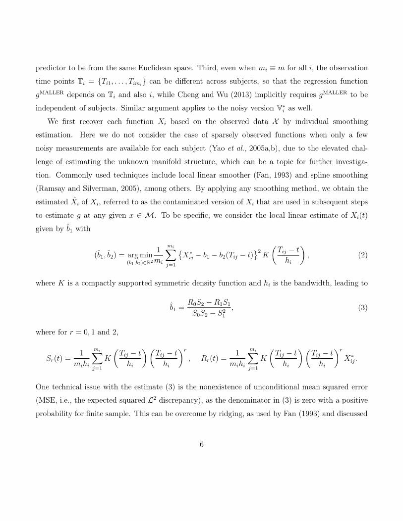
validation detailed in Cheng and Wu (2013). We emphasize that, in the above estimation procedure

which is illustrated by a diagram in the left panel of Figure 1, all steps are based on the contaminated

sample {X1, . . . , Xn}, rather than the unavailable functions Xi.

In practice, the predictor x is often not fully observed either. Instead, it is measured at mx

discrete points t1, . . . , tmx , and the measurements are corrupted by random noise. In this case, we

then estimate x by the same local linear smoothing method as in (2). We denote this estimate by

x, and replace x with x in (5)–(7) to obtain an estimate of g(x).

8

x

estimated TxM

proje

ctio

n

LLS on projected coordinates

observed (Xi’s)projected (xi’s)

manifold M

ϕ1

ι∗φ1

ι ∗φ2

tangent space TxM

OP(h

pca)u

⊥

OP(h3/

2

pca)u

Figure 1: Left: illustration of functional regression on manifold; Right: illustration of estimationquality of the tangent space at x.

3 Theoretical Properties

In this section, we investigate the theoretical properties of the estimate g(x) in (7). Recalling that

mi denotes the number of measurements for the predictor Xi, we assume that mi grows with sample

size n at a polynomial rate. Without loss of generality, assume mi ≍ m ≍ nα for some constant

α > 0, where an ≍ bn denotes 0 < lim inf an/bn < lim sup an/bn < ∞. The random noise ζij is

assumed to be i.i.d. for simplicity. It is worth pointing out that the development below can be

modified to accommodate weakly dependent and heterogeneous noise. This generality will introduce

considerably more tedious derivations without adding further insight, which is not pursued here.

The discrepancy between Xi and Xi, quantified by ‖Xi − Xi‖L2, is termed contamination of Xi.

It turns out that, the decay of this contamination is intimately linked to the consistency of the

estimates of the intrinsic dimension, the tangent spaces, and eventually the regression functional

g(x). As one of our main contributions, we discover that the convergence rate of g(x) exhibits a

phase transition phenomenon depending on the interplay between the intrinsic dimension and the

decay of contamination. We start with the property of contamination in recovery of functional data

to set the stage.

Recall that the individual smoothing to recover each Xi is based on the measurements available

for that individual, Xi = {(Ti1, X∗i1), (Ti2, X

∗i2), . . . , (Tim, X

∗im)}, so the estimates Xi are also i.i.d. if

9

the observed data are i.i.d., which simplifies our analysis and can be extended to weakly dependent

Xi without substantial changes. Specifically, we study the pth moment of contamination in L2 norm

when Xi is the ridged local linear estimate given by (4), while Fan (1993) derived the convergence

rate of ‖Xi −Xi‖2L2 conditional on Xi, , i.e., a special case of p = 2. As a matter of fact, our result

below for an arbitrary pth moment is not present in the literature.

Let Σ(ν, L) denote the Hölder class with exponent ν and Hölder constant L, which represents

the set of ℓ = ⌊ν⌋ times differentiable functions F whose derivative F (ℓ) satisfies |F (ℓ)(t)−F (ℓ)(s)| ≤L|t − s|ν−ℓ for s, t ∈ D, where ⌊ν⌋ is the largest integer strictly smaller than ν. We require mild

assumptions as follows, and assume hi ≍ h0 without loss of generality.

(A1) K is a differentiable kernel with a bounded derivative,´ 1

−1K(u)du = 1,

´ 1

−1uK(u)du =

0, and´ 1

−1|u|pK(u)du <∞ for all p > 0.

(A2) The sampling density fT is bounded away from zero and infinity, i.e., for some constants

CT,1, CT,2 ∈ (0,∞), CT,1 = inft∈D fT (t) ≤ supt∈D fT (t) = CT,2.

(A3) X ∈ Σ(ν, LX), where LX > 0 is a random quantity and 0 < ν ≤ 2 is some constant that

quantifies the smoothness of the process.

(A4) For all r ≥ 1, E supt |X(t)|r <∞, E(LX)r <∞ and E|ζ |r <∞.

Note that E supt |X(t)|r <∞ holds rather generally, as discussed in Li and Hsing (2010); Zhang and Wang (2016),

compared to a stronger assumption on X given in (A.1) of Hall et al. (2006). The following propo-

sition is an immediate consequence of Lemma S.1 in the Supplementary Material, and hence its

proof is omitted.

Proposition 1 For any p ≥ 1, assume E|ζ |p <∞. Under assumptions (A1)–(A3), for the estimate

X in (4) with h0 ≍ m− 1

2ν+1 and a proper choice of δ, we have

{E(‖X −X‖pL2 | X)}1/p = O(m− ν2ν+1 )

{

supt

|X(t)|+ LX

}

. (8)

10

Furthermore, if additionally assumption (A4) holds and m ≍ nα for some α > 0, then

(

E‖X −X‖pL2

)1/p

= O(n− αν2ν+1 ).

When X is deterministic as in nonparametric regression, the rate in (8) for p = 2 coincides with

that in Tsybakov (2008). Note that the pth order of the contamination ‖Xi − Xi‖L2 decays at a

polynomial rate which depends on the sampling rate α and smoothness ν, but not the order of p.

To analyze the asymptotic property of g(x), we make following assumptions.

(B1) The probability density f of X on M satisfies Cf,1 = infx∈M f(x) ≤ supx∈M f(x) = Cf,2

for some constants 0 < Cf,1 ≤ Cf,2 <∞.

(B2) The regression functional g is twice differentiable with a bounded second derivative.

(B3) X1, X2, . . . , Xn are independently and identically distributed. For some β ∈ (0,∞) and

all p ≥ 1, {E(‖X−X‖pL2 | X)}1/p ≤ Cpn−βη(X) for some constant Cp depending only on

p and some nonnegative function η(X) depending only on X such that E{η(X)}p <∞.

For (B1), since the predictor functions resides on a low-dimensional manifold, the existence of

a density can be safely assumed. Note that the assumption (B3) is presented in terms of the

contaminated predictor X, and hence implicitly poses requirement for the smoothing method. Under

assumptions (A1)–(A4), by Proposition 1, the individual smoothing via local linear estimation (4)

satisfies (B3) with β = αν/(2ν + 1). To give an intuitive interpretation, we define γ = β−1 =

(2+ ν−1)/α as the contamination level of X. We see that the contamination level is low for densely

observed (i.e., large α) or smoother (i.e., large ν) functions. We emphasize that our theory on the

estimated regression functional g does not depend on the smoothing method used in recovering

Xi, as long as (B3) is fulfilled. Further, we may extend (B3) to allow weak independence and

heterogeneous distribution of {X1, . . . , Xn} by modifying proofs. This will accommodate weakly

dependent functional data or the contaminated Xi that are attained by borrowing information

11

across individuals (e.g. Yao et al., 2005a), which is beyond our scope here and can be a topic of

future research.

The contamination of the predictor X poses substantial challenge on the estimation of the man-

ifold structures. For instance, the quality of the tangent space at x, denoted by TxM, crucially

depends on a bona fide neighborhood around x, while the contaminated neighborhood NL2(hpca, x)

and the inaccessible true neighborhood NL2(hpca, x) = {Xi : ‖Xi − x‖L2 < hpca} might contain

different observations. Fortunately we can show that they are not far apart in the sense of Propo-

sition S.2 in the Supplementary Material. In practice, we suggest to choose max(hreg, hpca) <

min{2/τ, inj(M)}/4, where τ is the condition number of M and inj(M) is the injectivity radius of

M (Cheng and Wu, 2013), so that NL2(hpca, x) provides a good approximation of the true neigh-

borhood of x within the manifold. The following result concerns the estimation quality of the local

manifold structures.

Theorem 1 Under assumptions (B1) and (B3), we have

(a) d is a consistent estimator of d when min{k1, k2} → ∞ and max{k1, k2}/n→ 0.

(b) Let = 1/(d+2) if β ≥ 2/d and = β/2 otherwise, hpca ≍ n−. Then the eigenbasis {ϕk}dk=1

derived from Cx in (6) is close to an orthonormal basis {φk}dk=1 of TxM: if x ∈ M, for

k = 1, 2, . . . , d,

ϕk = φk +OP (h3/2pca)uk +OP (hpca)u

⊥k , (9)

where uk ∈ TxM, u⊥k ⊥ TxM, and ‖uk‖L2 = ‖u⊥

k ‖L2 = 1.

In light of Theorem 1.(a), we shall from now on present the subsequent results by conditioning on

the event d = d, and the right panel of Figure 1 provides a geometric illustration of equation (9)

for the case d = 2. Note that, although the curvature at x does not appear in the asymptotic

rates in (9), it does play a role as a constant that is absorbed into the OP terms. The intuition

is that, no matter how large the curvature is at x, as long as it is fixed and bounded away from

infinity, the L2 distance can serve as a good approximation to the metric (distance) of objects on

12

the manifold M, provided that the distance of these objects is sufficiently small; e.g., Lemma A.2.3

of Cheng and Wu (2013). In practice, it is usually more difficult to estimate the tangent structure

at a point with larger curvature.

We are ready to state the results on the estimated regression functional. Recall that g(x) in (7)

is obtained by applying local linear smoother on the coordinates of contaminated predictors within

the estimated tangent space at x. It is well known that local linear estimator does not suffer from

boundary effects, i.e., the first order behavior of the estimator at the boundary is the same as in the

interior (Fan, 1992). However, the contamination on predictor has different impact, and we shall

address the interior and boundary cases separately. Denote X = {(X1, X1), (X2, X2), . . . , (Xn, Xn)}and Mh = {x ∈ M : infy∈∂M d(x, y) ≤ h}, where ∂M denotes the boundary of M and d(·, ·)denotes the distance function on M. For points sufficiently far away from the boundary of M, we

have the following result about the conditional mean square errors (MSE) of the estimate g(x).

Theorem 2 Assume that (A1) and (B1)–(B3) hold. Let x ∈ M\Mhreg and hpca chosen as in

Theorem 1((b)). For any ǫ > 0, if we choose hreg ≍ n−1/(d+4) when β > 3/(d + 4), and hreg ≍n−β/(3+ǫd) when β ≤ 3/(d+ 4), then

E[

{g(x)− g(x)}2 | X]

= OP

(

n− 4

d+4 + n− 4β3+ǫ

)

. (10)

We emphasize the following observations from this theorem. First, the convergence rate of g(x) is a

polynomial of the sample size n depending on both the intrinsic dimension d and the contamination

level defined as γ = β−1. This is in contrast with traditional functional nonparametric regression

methods that do not explore the intrinsic structure, which cannot reach a polynomial rate of conver-

gence. Second, when contamination level γ < γ0 = (d+4)/3, the intrinsic dimension dominates the

convergence rate in (10), while when γ ≥ γ0, the contamination dominates. Thus the convergence

rate exhibits a phase transition separated at the threshold level γ0. Intuitively, when the contam-

ination is low, the manifold structure can be estimated reliably and hence determines the quality

of the estimated regression. On the other hand, when the contamination passes the threshold γ0,

13

the manifold structure is buried by noise and cannot be well utilized. Third, it is observed that the

phase transition threshold γ0 increases with the intrinsic dimension d that indicates the complexity

of a manifold. This interesting finding suggests that, although estimating a complex manifold is

more challenging (i.e., slower rate), such a manifold is more resistant to contamination.

Theorem 2 can be also interpreted by relating the sampling rate m and the sample size n. Recall

that m ≥ nα and γ = (2 + ν−1)/α, where ν denotes the Hölder smoothness of the process X as

in (A3). When the sampling rate is low, α ≤ 3(2 + ν−1)/(d + 4), i.e., m . n3(2+ν−1)/(d+4), the

contamination reflected by the second term in the right hand side (r.h.s.) of (10) dominates and is

actually determined by m. Otherwise the first term prevails and involves only the sample size n and

the intrinsic dimension prevails. In the literature of functional data analysis, ν is typically at least 2,

i.e., continuously twice differentiable. For a moderate dimension such as d = 6, the contamination

blurs the estimation of g when m . n3/4, and becomes asymptotically negligible otherwise, where

an . bn denotes an/bn → 0.

The above interpretation clearly separates our theory from that in Cheng and Wu (2013) where

the actual observed predictor comes from a finite and fixed dimensional Euclidean space without

noise. In the functional setup, actual observed predictor is Xi = {(Ti1, X∗i1), (Ti2, X

∗i2), . . . , (Tim, X

∗im)}

(under assumption mi ≡ m), which is an m-dimensional vector whose distribution is fully supported

on Rm due to the presence of noise ζij, rather than a low-dimensional subspace of Rm. This im-

plies that the support of the distribution of Xi is also m-dimensional. The smoothness structure of

functional data could help tighten the distribution of Xi, but does not reduce its dimension. Thus,

as m goes to infinity, it might raise a serious concern of curse of dimensionality. In this sense, the

polynomial rate and phase transition phenomenon in Theorem 2 is nontrivial: when m is small

relative to the sample size n, it determines the convergence rate, while when it surpasses certain

threshold, by explicitly exploring the low-dimensional manifold structure, the growing dimension of

the contamination can be defeated with the aid of smoothness, so that m does not play a role any

more in the convergence rate. Next theorem characterizes the asymptotic behavior of g at x close

to the boundary of M.

14

Theorem 3 Assume that (A1) and (B1)–(B3) hold. Let x ∈ Mhreg and hpca chosen as in Theorem

1. For any ǫ > 0, if we choose hreg ≍ n−1/(d+4) when β > 4/(d + 4), and hreg ≍ n−β/(4+ǫd) when

β ≤ 4/(d+ 4), then the conditional MSE satisfies

E[

{g(x)− g(x)}2 | X]

= OP

(

n− 4

d+4 + n− 4β4+ǫ

)

. (11)

It is interesting to note that the effect of the intrinsic dimension on convergence is the same,

regardless where g is evaluated on the manifold. However, the effect of contamination behaves

differently, due to the fact that the second order behavior of local linear estimator that depends

on the location needs to be taken into account when there is contamination on X. We see that

when contamination effect dominates, the convergence is slightly slower for boundary points than

for interior points, and the phase transition occurs at γ0 = (d + 4)/4. This is the price we pay for

the boundary effect when predictors are contaminated, which is in contrast with the classical result

on local linear estimator (Fan, 1993).

Finally, we address the case that the predictor x is not fully observed. It is reasonable to assume

that x comes from the same source of the data, in the sense that its smoothed version x has the

same contamination level as those X1, . . . , Xn, as per (B3). To be specific, assume that

(B4) the estimate x is independent of X1, . . . , Xn and X1, . . . ,Xn. Also {E‖x − x‖pL2}1/p ≤C ′

pn−β for all p ≥ 1, where C ′

p is constant depending on p only.

Note that the independent condition in (B4) is satisfied if t1, . . . , tmx are independent of X1, . . . , Xn

and X1, . . . ,Xn. The second part of (B4) is met if assumptions similar to (A1)-(A4) hold also for x

and t1, . . . , tmx , according to Proposition 1.

Theorem 4 With conditions (A1), (B1)-(B3), and additional assumption (B4), equation (10) holds

when x ∈ M\Mhreg, and equation (11) holds when x ∈ Mhreg, both with g(x) replaced by g(x).

15

4 Simulation Study

To demonstrate the performance of our FREM framework, we conduct simulations for three different

manifold structures, namely, the three-dimensional rotation group SO(3), the Klein bottle (Klein)

and the mixture of two Gaussian densities (MixG). For all settings, a functional predictor Xi is

observed at m = 100 equally spaced points T1, T2, . . . , Tm in the interval [0, 1] with heteroscedastic

measurement error ǫij ∼ N(0, σ2j ), where σj is determined by the signal-to-noise ratio on X(Tj) so

that snrdbX = Var{X(Tj)}/σ2j = 4. The response is generated by Yi = 4 sin(4Zi) cos(Z

2i ) + 2Γ(1 +

Zi/2) + εi with Zi =´ 1

0X2

i (t)tdt and Γ(α) =´∞

0sα−1e−sds the gamma function. The noise εi on

response Y is a centered Gaussian variable with variance σ2ε that is determined by the signal-to-noise

ratio on Y so that snrdbY = Var(Y )/σ2ε = 2. Other information of each stetting is provided below.

• SO(3): Xi(t) =∑9

k=1 ξikbk(t), where φ2ℓ−1(t) = cos{(2ℓ−1)πt/10}/√5 and φ2ℓ(t) = sin{(2ℓ−

1)πt/10}/√5. To generate random variables ξik, we define vector r = (r1, r2, r3) and matrix

R(r, θ) = (1− cos θ)rrT +

cos θ −r3 sin θ r2 sin θ

r3 sin θ cos θ −r1 sin θ−r2 sin θ r1 sin θ cos θ

.

Denote e2 = (1, 0, 0)T and similarly e3, and we generate (ξi1, . . . , ξi9)T = vec(Zi) with

Zi = R(e3, ui)R(e2, vi)R(e3, wi), (12)

where (ui, vi) are i.i.d. random pairs uniformly distributed on the 2D sphere S2 = [0, 2π) ×[0, π], and wi are i.i.d. uniformly distributed on the unit circle S1 = [0, 2π). Note that

(12) is the Euler angles parameterization of SO(3) (Stuelpnagel, 1964) that has an intrinsic

dimension d = 3.

• Klein: Xi(t) =∑4

k=1 ξikφk(t) with φk as in the SO(3) setting. For random variables ξk,

we use ξi1 = (2 cos vi + 1) cosui, ξi2 = (2 cos vi + 1) sin ui, ξi3 = 2 sin vi cos(ui/2) and ξi4 =

16

2 sin vi sin(ui/2), where ui, vii.i.d.∼ Unif(0, 2π). Here (u, v) 7→ (ξ1, ξ2, ξ3, ξ4) is a parametrization

of Klein bottle with an intrinsic dimension d = 2.

• MixG: Xi is a mixture of two Gaussian densities, i.e., Xi(t) = exp{−(t − ui)2/2}/

√2π +

exp{−(t − vi)2/2}/

√2π with (v1, v2)

T uniformly sampled from a circle with diameter 0.5,

similar to that used in Chen and Müller (2012).

Note that, to see the impact of manifold structures on regression, we normalize the functional

predictor in all settings to the unit scale, i.e, multiplying X by the constant c = 1/√

E‖X‖2 so

that the resultant X satisfies E‖X‖2 = 1. Such scaling does not change the geometric structure

of manifolds but the size. In order to account for at least 95% of variance of the contaminated

data, we find empirically that more than 10 principal components are needed in all settings, i.e.,

the dimensions of the contaminated data are considerably larger than their intrinsic dimensions.

For each setting, three different sample sizes are considered, n = 250, n = 500 and n = 1000.

For evaluation, we generate independent test data of size 5000, and compute the square-root of

mean square error (rMSE) using the test data. It is noted that in the test data, each predictor

is also discretely measured and contaminated by noise in the same way of the training sample.

For comparison, we compute the rMSE for various functional nonparametric regression methods

described in Ferraty and Vieu (2006): functional Nadaraya-Watson estimator (FNW), functional

conditional expectation (FCE), functional mode (FMO), functional conditional median (FCM) and

the multi-method (MUL) that averages estimates from FCE, FMO and FCM. Functional linear

regression (FLR) is also included to illustrate the impact of nonlinear relationship not captured by

FLR. The tuning parameters in these methods, such as the number of principal components for

FLR and the bandwidth for FNW, FCE, FMO and FCM, are selected by 10-fold cross validation.

We repeat each study 100 times independently, and the results are presented in Table 4.

First, we observe that FREM enjoys favorable numerical performance in all simulation settings.

Second, as sample size grows, the reduction in rMSE is more prominent for FREM than for the

other methods. Take FNW and FREM in the Klein setting for example. The relative rMSE

reduction from n = 250 (n = 500, respectively) to n = 500 (n = 1000, respectively) is 25.5%

17

Table 1: Shown are the Monte Carlo averages of square-root mean square error (rMSE) and itsstandard error in parenthesis based on 100 independent simulation runs, for different settings andmethods described in Section 4, in the scale of 10−1.

SO(3) Klein Bottle MixGn = 250 n = 500 n = 1000 n = 250 n = 500 n = 1000 n = 250 n = 500 n = 1000

FLR 2.21(.034) 2.18(.023) 2.16(.020) 6.13(.062) 6.12(.039) 6.09(.035) 2.96(.143) 2.90(.126) 2.88(.099)FNW 1.62(.058) 1.57(.043) 1.55(.032) 3.18(.405) 2.91(.179) 2.83(.068) 1.87(.146) 1.75(.083) 1.70(.065)FCE 1.53(.066) 1.41(.052) 1.32(.030) 2.97(.146) 2.71(.104) 2.61(.081) 2.11(.132) 2.04(.093) 1.98(.064)FMO 2.54(.116) 2.30(.094) 2.20(.085) 4.62(.307) 4.12(.220) 3.83(.187) 3.59(.280) 3.36(.205) 3.22(.161)FCM 2.02(.060) 1.86(.052) 1.72(.035) 3.91(.267) 3.39(.161) 3.09(.102) 2.73(.171) 2.51(.105) 2.32(.083)MUL 1.82(.059) 1.66(.048) 1.54(.031) 3.40(.213) 3.00(.124) 2.77(.092) 2.46(.149) 2.31(.107) 2.18(.081)

FREM 1.01(.072) .816(.056) .638(.025) 1.65(.139) 1.23(.111) .951(.074) 1.05(.132) .808(.086) .612(.075)

(22.7%, respectively) for FREM, and 8.49% (2.75%, respectively) for FNW. This may provide

some numerical evidence that the proposed FREM has a faster convergence rate compared to its

counterparts (Mas, 2012). Furthermore, it also provides evidence for the polynomial rate stated

in Theorem 2–4, based on which the relative reduction is expected to be 1 − (n1/n2)2/(d+4) with

sample size from n1 to n2. For Klein setting, it is about 20.6%, and the empirical relative reduction

is 22.7% from n1 = 500 to n2 = 1000. Similar observations can be made for other settings.

In contrast, the existing kernel methods perform no better than a logarithmic rate, providing

numerical evidence for the theory of Mas (2012). Take FNW as example. The empirical relative

reduction is 2.75% from n1 = 500 to n2 = 1000, even less than what the logarithmic rate suggests,

1 − log(500)/ log(1000) ≈ 10.0%. Third, as the intrinsic dimension goes up, the relative rMSE

reduction for FREM decreases, suggesting that the intrinsic dimension plays an important role in

convergence rate. Finally, different manifold structures result in different constants hidden in the

OP terms in Theorem 2 and 3, e.g., those in the SO(3) setting are relatively smaller than their

counterparts in the Klein setting, which agrees with the empirical results.

18

Table 2: Shown are the relative reduction of rMSE in percentage.

SO(3) Klein Bottle MixG250 → 500 500 → 1000 250 → 500 500 → 1000 250 → 500 500 → 1000

FLR 1.36 .917 .163 .490 2.02 .690FNW 3.09 1.27 8.49 2.75 6.42 2.86FCE 7.84 6.38 8.75 3.69 3.32 2.94FMO 9.45 4.35 10.8 7.04 6.41 4.17FCM 7.92 7.53 13.3 8.85 8.06 7.57MUL 8.79 7.23 11.8 7.67 6.10 5.63

FREM 19.2 21.8 25.5 22.7 23.0 24.3

5 Real Data Examples

We apply FREM to analyze two real datasets. For the purpose of evaluation, we train our method

on 75% of each dataset and reserve the other 25% as test data. The rMSE is computed on the

held-out test data. For comparison, we also compute rMSE for FLR, FNW, FCE, FMO and FCM

as described in Section 4. We repeat this 100 times based on random partitions of the datasets,

and present the Monte Carlo averages of rMSE together with their standard errors in Table 3.

The first application is to predict fat content of a piece of meat based on a spectrometric

curve of spectra of absorbances for the meat using the Tecator dataset with 215 meat samples

(Ferraty and Vieu, 2006). For each sample, the spectrometric curve for a piece of finely chopped

pure meat was measured at 100 different wavelengths from 850 to 1050nm. Along with spectromet-

ric curves, the fat content for each piece of meat was recorded. Comparing to the analytic chemistry

required for measuring the fat content, obtaining a spectrometric curve is less time and cost consum-

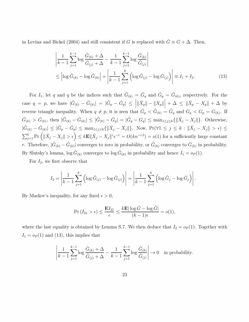
ing. As in Ferraty and Vieu (2006), we predict the fat content based on the first derivative curves

approximated by the difference quotient between measurements at adjacent wavelengths, shown

in the left panel of Figure 2. It is seen that there are some striking patterns around the middle

wavelengths. The proposed FREM is able to capture these patterns by a low-dimensional manifold

structure and yields more efficient estimates of fat content. For example, the FLR model uses 15.7

19

850 900 950 1000 1050−0.02

0

0.02

0.04

0.06

Abs

orba

nce

(1st

der

iv)

Wavelength20 40 60 80

0.2

0.3

0.4

0.5

0.6

0.7

0.8

Fra

ctio

nal A

niso

trop

y

Tract location

Figure 2: Left: first derivative curves of the spectra of absorbance for finely chopped 215 puremeat samples. Right: 340 fractional anisotropy profiles along corpus callosum tract location.

principal components on average with standard error 1.07, while the intrinsic dimension estimated

by FREM is 5.05 with a standard error 0.62. From Table 3, FREM predicts the fat content more

accurately than the other methods by a significant margin.

The second example studies the relationship between cognitive function and brain microstructure

in the corpus callosum of patients with multiple sclerosis (MS), a common demyelinating disease

caused by inflammation in the brain. It is observed that nerve cells are often covered by myelin,

an insulating material that protects axons and helps nerve signal to travel faster. Demyelination

refers to damage to myelin, which can result from immune-mediated inflammation, among other

causes. Demyelination occurring in the white matter of brain, from which MS patients suffer, can

potentially lead to loss of mobility or even cognitive impairment (Jongen et al., 2012). Diffusion

tensor imaging (DTI), a technique that can produce high-resolution images of white matter tissues

by tracing water diffusion within the tissues, is an important method to examine potential myelin

damage in the brain. For example, from the DTI images, some properties of white matter, such as

fractional anisotropy (FA) of water diffusion, can be derived. It has been shown that FA is related

to multiple sclerosis (Ibrahim et al., 2011).

To predict cognitive performance based on FA profiles for MS patients, we utilize the DTI

20

Table 3: Shown are the Monte Carlo averages of square-root mean square error (rMSE) and itsstandard error based on 100 random partitions, for different methods on the meat spectrometricdata and DTI data, where the results for DTI data is multiplied by 0.1 for visualization.

FLR FNW FCE FMO FCM MUL FREM

Meat 2.56(.433) 2.42(.334) 1.97(.354) 2.66(.459) 2.82(.454) 2.31(.354) 1.06(.344)DTI 1.14(.092) 1.28(.115) 1.36(.126) 1.78(.158) 1.25(.141) 1.33(.126) .961(.089)

data collected at Johns Hopkins University and the Kennedy-Krieger Institute. The data contains

n = 340 FA profiles from MS patients and Paced Auditory Serial Addition Test (PASAT) scores that

quantify cognitive function (Gronwall, 1977), where each FA profile is recorded at a grid of 93 points.

In the right panel of Figure 2, we show all FA profiles, and observe that the data is considerably more

complex than the spectrometric data. The average of estimated intrinsic dimensions is 5.82 with

standard error 0.098. By contrast, the average number of principal components for FLR is 11.98

with standard error 5.22. According to Table 3, our method enjoys the most accurate prediction,

followed by the FLR, while all other functional nonparametric methods deteriorate substantially.

SUPPLEMENTARY MATERIAL

Auxiliary results and technical lemmas with proofs, as well as the proof of Theorem 3 (similar

to the proof of Theorem 2) are collected in an online Supplementary Material for space economy.

ACKNOWLEDGMENTS

This research is partially supported by Natural Science and Engineering Research Council of

Canada.

Example and Proofs of Theorems

For illustration purpose, we present below a one-dimensional submanifold of L2([0, 1]) and a random

process taking value in this manifold while having an infinite number of components in its Karhunen-

21

Loève expansion. Note that examples for dimensions larger than one can be constructed in a similar

fashion.

Example 1 Let S1 = {vω = (cosω, sinω) : ω ∈ [0, 2π)} denote the unit circle regarded as a one-

dimensional Riemannian manifold. Let D = [0, 1] and denote φ1, φ2, . . . a complete orthonormal

basis of L2(D). Define map X(vω) =√C∑

k k−c{cos(kω)φ2k−1+sin(kω)φ2k} with c > 3/2 and C =

1/∑

k k−2c+2 ∈ (0,∞). According to Proposition S.1 in Supplementary Material, X is an isometric

embedding of S1 into L2(D). Then M = X(S1) is a submanifold of L2(D). Moreover, no finite-

dimensional linear subspace of L2(D) fully encompasses M. A consequence of this observation is

that, a random process taking samples from such M might have an infinite number of eigenfunctions,

even though M is merely one-dimensional, as we shall exhibit in the following. Let us treat S1

as a probability space endowed with the uniform probability measure, and define random variables

ξ2k−1(vω) =√Ck−c cos(kω) and ξ2k(vω) =

√Ck−c sin(kω). Then X =

∑

k ξkφk can be regarded as

a random process with samples from M. It is easy to check that E(ξkξj) = 0 if k 6= j, E(ξk) =

0, and Eξ22k−1 = Eξ22k = Cπk−2c, which implies that E(‖X‖2L2) < ∞. One can see that the

eigenfunctions of the covariance operator of X are exactly φk. Therefore, X =∑

k ξkφk is the

Karhunen-Loève expansion of the random process X, which clearly includes an infinite number of

principal components, while X is intrinsically sampled from the one-dimensional manifold M.

Below we shall provide proofs for Theorem 1 and 2, while the proof of Theorem 3 using similar

techniques is deferred to the Supplementary Material. To reduce notational burden, L2(D) is

simplified by L2, and we shall use ‖ · ‖ to denote the norm ‖ · ‖L2 when no confusion arises.

Proof of Theorem 1. (a) Without loss of generality, assume x = 0. Let Gj = Gj +∆ and

G(1), G(2), . . . , G(k) be the associated order statistics of G1, G2, . . . , Gk. Also note that the estimator

22

in Levina and Bickel (2004) and still consistent if G is replaced with G ≡ G +∆. Then,

∣

∣

∣

∣

∣

1

k − 1

k−1∑

j=1

logG(k) +∆

G(j) +∆− 1

k − 1

k−1∑

j=1

logG(k)

G(j)

∣

∣

∣

∣

∣

≤∣

∣

∣log G(k) − log G(k)

∣

∣

∣+

∣

∣

∣

∣

∣

1

k − 1

k∑

j=1

(

log G(j) − log G(j)

)

∣

∣

∣

∣

∣

≡ I1 + I2. (13)

For I1, let q and q be the indices such that G(k) = Gq and Gp = G(k), respectively. For the

case q = p, we have |G(k) − G(k)| = |Gp − Gp| ≤∣

∣

∣‖Xp‖ − ‖Xp‖

∣

∣

∣+ ∆ ≤ ‖Xp − Xp‖ + ∆ by

reverse triangle inequality. When q 6= p, it is seen that Gp < G(k) = Gq and Gq < Gp = G(k). If

G(k) > G(k), then |G(k) − G(k)| ≤ |G(k) − Gq| = |Gq − Gq| ≤ max1≤j≤k{‖Xj − Xj‖}. Otherwise,

|G(k) − G(k)| ≤ |Gp − Gp| ≤ max1≤j≤k{‖Xj − Xj‖}. Now, Pr(∀1 ≤ j ≤ k : ‖Xj − Xj‖ > ǫ) ≤∑k

j=1Pr(

‖Xj −Xj‖ > ǫ)

≤ kE‖Xj −Xj‖rǫ−r = O(kn−rβ) = o(1) for a sufficiently large constant

r. Therefore, |G(k) − G(k)| converges to zero in probability, or G(k) converges to G(k) in probability.

By Slutsky’s lemma, log G(k) converges to log G(k) in probability and hence I1 = oP (1).

For I2, we first observe that

I2 =

∣

∣

∣

∣

∣

1

k − 1

k∑

j=1

(

log G(j) − log G(j)

)

∣

∣

∣

∣

∣

=

∣

∣

∣

∣

∣

1

k − 1

k∑

j=1

(

log Gj − log Gj

)

∣

∣

∣

∣

∣

.

By Markov’s inequality, for any fixed ǫ > 0,

Pr (I21 > ǫ) ≤ EI21ǫ

≤ kE| log G− log G|(k − 1)ǫ

= o(1),

where the last equality is obtained by Lemma S.7. We then deduce that I2 = oP (1). Together with

I1 = oP (1) and (13), this implies that

∣

∣

∣

∣

∣

1

k − 1

k−1∑

j=1

logG(k) +∆

G(j) +∆− 1

k − 1

k−1∑

j=1

logG(k)

G(j)

∣

∣

∣

∣

∣

→ 0 in probability.

23

Now we apply the argument in Levina and Bickel (2004) to conclude that d is a consistent estimator.

(b) Let h = hpca, and {φk}dk=1 be a orthonormal basis system for TxM and {ψk}∞k=1 be an or-

thonormal basis of L2. Without loss of generality, assume that M is properly rotated and translated

so that ψk = φk for k = 1, 2, . . . , d, and x = 0 ∈ L2. The sample covariance operator based on ob-

servations in NL2(h, x) is denoted by Cx as in (6). It is seen that Cx = n−1∑n

i=1(Xi−µx)(Xi−µx)Zi,

where Zi = 1{Xi∈BL2

h (x)}and µx = n−1

∑ni=1 XiZi. Let H1 = span{ψk : k = 1, 2, . . . , d} and H2 be

the complementary subspace of H1 in L2, so that L2 = H1 ⊕H2. Let Pj : L2 → Hj be projection

operators, and we define operator A = P1CxP1, B = P2CxP2, D12 = P1CxP2 and D21 = P2CxP1.

Then Cx = A+B+D12+D21. Note that D12+D21 is self-adjoint. Therefore, if y =∑∞

k=1 akψk ∈ L2,

‖D12 +D21‖op = sup‖y‖=1

〈(D12 +D21)y, y〉 = sup‖y‖=1

(

〈P1CxP2y, y〉+ 〈P2CxP1y, y〉)

=2 sup‖y‖=1

(

∞∑

k=d+1

d∑

j=1

ajak〈Cxψj , ψk〉)

≤ 2 sup‖y‖=1

(

∞∑

k=d+1

d∑

j=1

|ajak| ·∣

∣

∣〈Cxψj , ψk〉

∣

∣

∣

)

≤2 supj≤d

supk≥d+1

∣

∣

∣〈Cxψj , ψk〉

∣

∣

∣sup‖y‖=1

{

∞∑

k=d+1

d∑

j=1

(a2j + a2k)

}

≤ 2 supj≤d

supk≥d+1

∣

∣

∣〈Cxψj , ψk〉

∣

∣

∣.

From Lemma S.9, ‖D12+D21‖op = OP

(

hd+3 + n−1/2hd/2+3 + n−βhd+1)

. Similarly, we have ‖B‖op =OP

(

hd+4 + n−1/2hd/2+4 + n−βhd+1)

, and A = πd−1f(x)d−1hd+2Id + OP

(

n−1/2hd/2+2 + n−βhd+1)

,

where πd−1 is the volume of d− 1 dimensional unit sphere, and Id is the identity operator on H1.

By assumption on , we have < min{1/d, β}. Then hd+2 is the dominant term. Let an =

n−1/2h−d/2 and bn = n−βh−1, we have

Cx = πd−1f(x)d−1hd+2{Id +OP (an + bn) A+OP

(

h2 + bn)

B +OP (h+ bn) (D12 + D21)}

where A, B, D12 and D21 are all with operator norm equal to one, and D12 is the adjoint of D21. With

the choice of , we have Cx = πd−1f(x)d−1hd+2

{

Id +OP (√h)A+OP (h)B +OP (h)(D12 + D21)

}

.

The same perturbation argument done in Singer and Wu (2012) leads to the desired result. �

24

Proof of Theorem 2. The proof is analogous to that of Theorem 4.2 of Cheng and Wu (2013),

except that we need to handle the extra difficulty caused by noise on X. For clarity, we give a

self-contained proof with emphasis on the extra issues. To reduce notions, let h = hreg and fix

x ∈ M\Mhreg. Let {ϕk}dk=1 be the orthonormal set determined by local FPCA and {φk}dk=1 the

associated orthonormal basis of TxM. Let {ψk}∞k=1 be an orthonormal basis of L2. Without loss

of generality, assume M is properly rotated and translated so that x = 0 ∈ L2 and ψk = φk for

k = 1, 2, . . . , d. Let g = (g(X1), g(X2), . . . , g(Xn))T . Then we have

E{g(x) | X } = eT1 (XTWX)−1XTWg.

Take z = expx(tθ), where t = O(h), θ ∈ TxM, ‖θ‖L2 = 1, and expx denotes the exponential map

of M at x. By Theorem 1, we have 〈θ, ϕk〉 = 〈θ, ψk〉+OP (h3/2pca) and 〈Πx(θ, θ), ϕk〉 = OP (hpca). By

Lemma A.2.2. of Cheng and Wu (2013), we have

tθ = y − t2Πx(θ, θ)/2 +O(t3). (14)

Therefore, for k = 1, 2, . . . , d, 〈tθ, ψk〉 = 〈tθ, ϕk − OP (h3/2pca)uk〉 = 〈z, ϕk〉 − t2〈Πx(θ, θ), ϕk〉/2 +

OP (hh3/2pca + h2hpca) = 〈z, ϕk〉 + OP

(

hh3/2pca + h2hpca

)

. Since θ ∈ TxM, we have θ =∑d

k=1〈θ, ψk〉φk.

Let z = (〈z, ϕ1〉, 〈z, ϕ2〉, . . . , 〈z, ϕd〉)T . By (14), it is easy to see that

g(x)− g(z) = tθ∇g(x) + Hess g(z)(θ, θ)t2/2 +OP (t3)

=

d∑

k=1

〈tθ, ψk〉∇φkg(z) +

1

2

d∑

j,k=1

〈tθ, ψj〉〈tθ, ψk〉Hess g(z)(φj, φk) +OP (h3)

= zT∇g(x) + 1

2zTHess g(x)z+OP (h

5/2).

Due to smoothness of g, compactness of M and the compact support of K, we have g =

X[g(x) ∇g(x)]T +H/2+OP (h5/2), where H = [xT

1Hess g(x)x1,xT2Hess g(x)x2, . . . ,x

TnHess g(x)xn]

T .

25

Then the conditional bias is

E{g(x)− g(x) | X } = eT1 (XTWX)−1XTWg − g(x)

= eT1

(

1

nXTWX

)−11

nXTW(X− X)

g(x)

∇g(x)

(15)

+ eT1

(

1

nXTWX

)−11

nXTW

{

1

2H+OP (h

5/2)

}

. (16)

Now we analyze the term in (15). Let Z = 1X∈BL2

h (x). By Lemma S.8, EZ ≍ hd. Then, by

Hölder’s inequality, for any fixed ǫ > 0, we choose a constant q > 1 and a sufficiently large p > 0 so

that 1/q + 1/p = 1 and EZ‖X −X‖ = (EZ)1/q(E‖X −X‖p)1/p = O(hd−ǫdn−β). Therefore,

1

nXTW(X− X)

g(x)

∇g(x)

=

1n

∑ni=1Kh(‖Xi − x‖)(xi − xi)

T∇g(x)1n

∑ni=1Kh(‖Xi − x‖)(xi − xi)

T∇g(x)xi

= OP (h−1−ǫdn−β), (17)

since

∣

∣

∣

∣

∣

1

n

n∑

i=1

Kh(‖Xi − x)‖)(xi − xi)T∇g(x)

∣

∣

∣

∣

∣

≤ 1

n

n∑

i=1

Kh(‖Xi − x‖)‖xi − xi‖Rd‖∇g(x)‖

≤ {supv

|K(v)|}‖∇g(x)‖(

1

n

n∑

i=1

Zi‖xi − xi‖Rd

)

= OP (h−1−ǫdn−β),

and similarly, n−1∑n

i=1Kh(‖Xi − x‖)(xi − xi)T∇g(x)xi = OP (h

−1−ǫdn−β)1d×1.

For XTWX, a direct calculation shows that

1

nXTWX =

n−1∑n

i=1Kh(‖Xi − x‖) n−1∑n

i=1Kh(‖Xi − x‖)xTi

n−1∑n

i=1Kh(‖Xi − x‖)xi n−1∑n

i=1 xTi Kh(‖Xi − x)‖)xi

.

It is easy to check that n−1∑n

i=1Kh(‖Xi − x‖) = n−1∑n

i=1Kh(‖Xi − x‖) + OP (h−1−ǫdn−β), and

note that the choice of h ensures that h1+ǫd ≫ n−β . Similar calculation shows that 1n

∑ni=1Kh(‖Xi−

26

x‖)xTi = 1

n

∑ni=1Kh(‖Xi−x‖)xT

i +OP (h−1−ǫdn−β) and also 1

n

∑ni=1 x

Ti Kh(‖Xi−x)‖)xi =

1n

∑ni=1 x

Ti Kh(‖Xi−

x‖)xi +OP (h−1−ǫdn−β). Therefore,

1

nXTWX =

1

nXTWX+OP (h

−1−ǫdn−β)1d×11Td×1, (18)

with

1

nXTWX =

n−1∑n

i=1Kh(‖Xi − x‖) n−1∑n

i=1Kh(‖Xi − x‖)xTi

n−1∑n

i=1Kh(‖Xi − x‖)xi n−1∑n

i=1 xiKh(‖Xi − x‖)xTi

.

By Lemma S.4, S.5 and S.6, we have

1

nXTWX

=

f(x) h2u1,2d−1∇f(x)T

h2u1,2d−1∇f(x) h2u1,2d

−1f(x)Id

+

O(h2) +OP (n− 1

2h−d2 ) O(h3) +OP (n

− 1

2h−d2+1)

O(h3) +OP (n− 1

2h−d2+1) O(h7/2) +OP (n

− 1

2h−d2+2)

,

where uq,k are constants defined in Section S.2 of Supplementary Material. Therefore, combined

with (18), it yields

1

nXTWX =

f(x) h2u1,2d−1∇f(x)T

h2u1,2d−1∇f(x) h2u1,2d

−1f(x)Id

+

O(h2) +OP (n− 1

2h−d2 ) +OP (h

−1−ǫdn−β) O(h3) +OP (n− 1

2h−d2+1) +OP (h

−1−ǫdn−β)

O(h3) +OP (n− 1

2h−d2+1) +OP (h

−1−ǫdn−β) O(h7/2) +OP (n− 1

2h−d2+2) +OP (h

−1−ǫdn−β)

.

By our choice of h, we have h−1−ǫdn−β ≪ h2. Then, by binomial inverse theorem and matrix

27

blockwise inversion, we have

(

1

nXTWX

)−1

=

1f(x)

−∇T f(x)f(x)2

∇T f(x)f(x)2

h−2 du1,2f(x)

Id

+

OP (h2 + h−1−ǫdn−β + n− 1

2h−d2 ) OP (h+ h−3−ǫdn−β + n− 1

2h−d2−1)

OP (h+ h−3−ǫdn−β + n− 1

2h−d2−1) OP (h

− 1

2 + h−5−ǫdn−β + n− 1

2h−d2−2)

. (19)

Therefore, with (17), we conclude that

eT1 (XTWX)−1XTW

(X− X)

g(x)

∇g(x)

=OP (h−1−ǫdn−β). (20)

Now we analyze (16) with a focus on the term XTWH. A calculation similar to those in Lemma

S.5 and S.6 shows that 1n

∑ni=1Kh (‖Xi − x‖)xT

i Hess g(x)xi = h2u1,2d−1f(x)∆g(x) + OP (h

7/2 +

n−1/2h−d/2+2) and 1n

∑ni=1Kh (‖Xi − x‖)xT

i Hess g(x)xixi = OP (h4 + n− 1

2h−d2+3). Therefore,

1

nXTWH =

h2u1,2d−1f(x)∆g(x) +OP (h

7/2 + n−1/2h−d/2+2)

h4 + n− 1

2h−d2+3

and hence

1

nXTWH =

h2u1,2d−1f(x)∆g(x) +OP (h

7/2 + n−1/2h−d/2+2 + h−1−ǫdn−β)

OP (h4 + n− 1

2h−d2+3 + h−1−ǫdn−β)

.

The choice of h implies that n− 1

2h−d2 ≪ 1. Thus, with (19), eT1 (X

TWX)−1XTW{

12H+OP (h

3)}

=

12dh2u1,2∆g(x)+OP (h

3+n− 1

2h−d2+2+h−1−ǫdn−β). Combining this equation with (16) and (20) , we

immediately see that the conditional bias is

E{g(x)− g(x) | X } =1

2dh2u1,2∆g(x) +OP (h

3 + n− 1

2h−d2+2 + h−1−ǫdn−β). (21)

28

Now we analyze the conditional variance. Simple calculation shows that

Var{g(x) | X } = n−1σ2ζe

T1 (n

−1XTWX)−1(n−1XTWWX)(n−1XTWX)−1eT1 . (22)

It is easy to see that

1

nXTWWX =

1

nXTWWX+OP (n

−βh−d−1−ǫd)1(d+1)×(d+1). (23)

Also,

1

nXTWWX =

1n

∑ni=1K

2h (‖Xi − x‖) 1

n

∑ni=1K

2h (‖Xi − x‖)xT

i

1n

∑ni=1K

2h (‖Xi − x‖)xi

1n

∑ni=1K

2h (‖Xi − x‖)xix

Ti

.

With Lemma S.4, S.5 and S.6, we can show that

hd

nXTWWX

=

u2,0σ2f(x) h2d−1u2,2σ

2∇f(x)h2d−1u2,2σ

2∇Tf(x) h2d−1u2,2σ2f(x)Id

+

O(h2) +OP (n− 1

2h−d2 ) OP (h

3 + n− 1

2h−d2+1)

OP (h3 + n− 1

2h−d2+1) OP (h

7

2 + n− 1

2h−d2+2)

.

Combined with (19), the above equation implies that

n−1σ2ǫ e

T1 (n

−1XTWX)−1(n−1XTWWX)(n−1XTWX)−1eT1

=1

nhdu2,0σ

2ζ

f(x)+OP

(

n−1h−d(h−1−ǫdn−β + n− 1

2h−d2 ))

. (24)

Also,

n−1σ2ζe

T1 (n

−1XTWX)−11(d+1)×(d+1)(n−1XTWX)−1eT1OP (h

−d−1−ǫdn−β)

= OP

(

n−β−1h−d−1−ǫd(1 + h+ h−1−ǫdn−β + n− 1

2h−d2−1))

. (25)

Combining the above result with (22), (23), (24), (25) and the fact h2 ≥ h−1−ǫdn−β due to the

29

choice of h, gives the conditional variance

Var{g(x) | X } =1

nhdu2,0σ

2ζ

f(x)+OP

(

n−1h−d(h+ n− 1

2h−d2 ))

. (26)

Finally, the rate for E[{g(x)− g(x)}2 | X ] is derived from (21) and (26). �

Proof of Theorem 4. We first observe that

E[

{g(x)− g(x)}2 | X]

≤ 2E[

{g(x)− g(x)}2 | X]

+ 2E[

{g(x)− g(x)}2 | X]

.

To derive the order for the first term, we shall point out that, with Lemma S.7, S.8 and S.9, by

following almost the same lines of argument, conclusions of Theorem 1 hold for x. This means, by

working on x instead of x, we still have a consistent estimate of dimension and a good estimate of

tangent space at x. Given this, it is not difficult but somewhat tedious to verify that the argument

in the proof of Theorem 2 and 3 still holds for x, with care for the discrepancy ‖x − x‖L2 instead

of the discrepancy ‖Xi − Xi‖L2. This argument also shows that the order of the first term is the

same as the second one (this is expected since x has the same contamination level of those Xi), and

hence the conclusion of Theorem 4 follows. �

References

Aswani, A., Bickel, P. and Tomlin., C. (2011). Regression on manifolds: Estimation of the

exterior derivative. The Annals of Statistics 39 48–81.

Cai, T. and Yuan, M. (2011). Optimal estimation of the mean function based on discretely

sampled functional data: Phase transition. The Annals of Statistics 39 2330–2355.

Cardot, H., Ferraty, F. and Sarda, P. (1999). Functional linear model. Statistics & Probability

Letters 45 11–22.

Cardot, H. and Sarda, P. (2005). Estimation in generalized linear models for functional data

30

via penalized likelihood. Journal of Multivariate Analysis 92 24–41.

Chen, D. and Müller, H. (2012). Nonlinear manifold representations for functional data. The

Annals of Statistics 40 1–29.

Cheng, M. and Wu, H. (2013). Local linear regression on manifolds and its geometric interpreta-

tion. Journal of the American Statistical Association 108 1421–1434.

Cornea, E., Zhu, H., Kim, P. and Ibrahim, J. G. (2017). Regression models on Riemannian

symmetric spaces. Journal of the Royal Statistical Society, Series B 79 463–482.

Delaigle, A. and Hall, P. (2010). Defining probability density for a distribution of random

functions. The Annals of Statistics 38 1171–1193.

Fan, J. (1992). Design-adaptive nonparametric regression. Journal of the American Statistical

Association 87 998–1004.

Fan, J. (1993). Local linear regression smoothers and their minimax efficiencies. The Annals of

Statistics 21 196–216.

Ferraty, F., Keilegom, I. V. and Vieu, P. (2012). Regression when both response and predictor

are functions. Journal of Multivariate Analysis 109 10–28.

Ferraty, F. and Vieu, P. (2006). Nonparametric Functional Data Analysis: Theory and Practice.

Springer-Verlag, New York.

Gronwall, D. M. A. (1977). Paced auditory serial-addition task: A measure of recovery from

concussion. Perceptual and Motor Skills 44 367–373.

Hall, P. and Horowitz, J. L. (2007). Methodology and convergence rates for functional linear

regression. The Annals of Statistics 35 70–91.

Hall, P. and Hosseini-Nasab, M. (2006). On properties of functional principal components

analysis. Journal of the Royal Statistical Society: Series B (Statistical Methodology) 68 109–126.

Hall, P. and Marron, J. S. (1997). On the shrinkage of local linear curve estimators. Statistics

and Computing 516 11–17.

Hall, P., Müller, H. G. and Wang, J. L. (2006). Properties of principal component methods

31

for functional and longitudinal data analysis. The Annals of Statistics 34 1493–1517.

Ibrahim, I., Tintera, J., Skoch, A., F., J., P., H., Martinkova, P., Zvara, K. and Rasova,

K. (2011). Fractional anisotropy and mean diffusivity in the corpus callosum of patients with

multiple sclerosis: the effect of physiotherapy. Neuroradiology 53 917–926.

Jongen, P., Ter Horst, A. and Brands, A. (2012). Cognitive impairment in multiple sclerosis.

Minerva Medica 103 73–96.

Kong, D., Xue, K., Yao, F. and Zhang, H. H. (2016). Partially functional linear regression in

high dimensions. Biometrika 103 147–159.

Kudraszow, N. L. and Vieu, P. (2013). Uniform consistency of kNN regressors for functional

variables. Statistics & Probability Letters 83 1863–1870.

Lang, S. (1995). Differential and Riemannian Manifolds. Springer, New York.

Lang, S. (1999). Fundamentals of Differential Geometry. Springer, New York.

Levina, E. and Bickel, P. (2004). Maximum likelihood estimation of intrinsic dimension. Ad-

vances in Neural Information 17 777–784.

Li, Y. and Hsing, T. (2010). Uniform convergence rates for nonparametric regression and principal

component analysis in functional/longitudinal data. The Annals of Statistics 38 3321–3351.

Lila, E. and Aston, J. (2016). Smooth principal component analysis over two-dimensional man-

ifolds with an application to neuroimaging. The Annals of Applied Statistics 10 1854–1879.

Loh, P.-L. and Wainwright, M. J. (2012). High-dimensional regression with noisy and missing

data: Provable guarantees with non-convexity. The Annals of Statistics 40 1637–1664.

Mas, A. (2012). Lower bound in regression for functional data by representation of small ball

probabilities. Electronic Journal of Statistics 6 1745–1778.

Müller, H. G. and Stadtmüller, U. (2005). Generalized functional linear models. The Annals

of Statistics 33 774–805.

Müller, H. G. and Yao, F. (2008). Functional additive models. Journal of the American

Statistical Association 103 1534–1544.

32

Ramsay, J. O. and Silverman, B. (2002). Applied Functional Data Analysis: Methods and Case

Studies. Springer, New York.

Ramsay, J. O. and Silverman, B. W. (1997). Functional Data Analysis. Springer-Verlag, New

York.

Ramsay, J. O. and Silverman, B. W. (2005). Functional Data Analysis. Springer Series in

Statistics, 2nd edition. Springer, New York.

Seifert, B. and Gasser, T. (1996). Finite-sample variance of local polynomials: analysis and

solutions. Journal of the American Statistical Association 91 267–275.

Singer, A. and Wu, H.-T. (2012). Vector diffusion maps and the connection Laplacian. Commu-

nications on Pure and Applied Mathematics 65 1067–1144.

Stuelpnagel, J. (1964). On the parametrization of the three-dimensional rotation group. SIAM

Review 6 422–430.

Tenenbaum, J. B., de Silva, V. and Langford, J. C. (2000). A global geometric framework

for nonlinear dimensionality reduction. Science 290 2319–2323.

Tsybakov, A. B. (2008). Introduction to Nonparametric Estimation. Springer, New York.

Yao, F. and Müller, H. G. (2010). Functional quadratic regression. Biometrika 97 49–64.

Yao, F., Müller, H. G. and Wang, J.-L. (2005a). Functional data analysis for sparse longitu-

dinal data. Journal of the American Statistical Association 100 577–590.

Yao, F., Müller, H. G. and Wang, J.-L. (2005b). Functional linear regression analysis for

longitudinal data. The Annals of Statistics 33 2873–2903.

Yuan, M. and Cai, T. T. (2010). A reproducing kernel Hilbert space approach to functional linear

regression. The Annals of Statistics 38 3412–3444.

Yuan, Y., Zhu, H., Lin, W. and Marron, J. S. (2012). Local polynomial regression for sym-

metric positive definite matrices. Journal of Royal Statistical Society, Series B 74 697–719.

Zhang, X. and Wang, J.-L. (2016). From sparse to dense functional data and beyond. The

Annals of Statistics 44 2281–2321.

33

Zhou, L. and Pan, H. (2014). Principal component analysis of two-dimensional functional data.

Journal of Computational and Graphical Statistics 23 779–801.

34

20 40 60 800.2

0.3

0.4

0.5

0.6

0.7

0.8

Fra

ctio

nal A

niso

trop

y

Tract location

850 900 950 1000 10502

3

4

5

6

Abs

orba

nce

Wavelength

arX

iv:1

704.

0300

5v3

[st

at.M

E]

12

Apr

201

9

Supplementary Material for “Functional Regression on

Manifold with Contamination”

Zhenhua Lin∗ Fang Yao∗†

S.1 Auxiliary Results

For convenience, in the sequel we might simplify L2(D) by L2, and use ‖ · ‖ to denote the norm

‖ · ‖L2 when no confusion arises.

Proposition S.1. The embedding X defined in Example 1 is an isometric embedding. Moreover,

there is no finite-dimensional linear subspace of L2(D) that fully contains the image X(S1).

Proof. Let V = {(cosω, sinω) : ω ∈ (a, b)} be a local neighborhood of v, and let ψ(v) = ω ∈(a, b) for v = (v1, v2) = (cosω, sinω) ∈ V . Then ψ is a chart of S1. Let U be open in L2 such that

X(v) ∈ U . Since L2 is a linear space, the identity map I serves as a chart. Let XU,V : ψ(V ) → L2

denote the map X ◦ ψ−1. Let ϑ =√C∑

k k−c+1{− sin(kω)φ2k−1 + cos(kω)φ2k}. It defines a linear

∗Department of Statistics, University of California, Davis.†Department of Probability and Statistics, Peking University. Email: fyao@utstat.toronto.edu

1

map from R to L2, denoted by Θ(t) = tϑ ∈ L2. Then,

A(t) ≡t−2‖XU,V (ω + t)−XU,V (ω)−Θ(t)‖2

=C∞∑

k=1

{

k−c cos(kω + kt)− k−c cos(kω) + tk−c+1 sin(kω)

t

}2

+

C

∞∑

k=1

{

k−c sin(kω + kt)− k−c sin(kω)− tk−c+1 cos(kω)

t

}2

≡CB21(t) + CB2

2(t).

By Lipschitz property of the function

B1,k(t) ≡ k−c cos(kω + kt)− k−c cos(kω) + tk−c+1 sin(kω),

we conclude that |B1,k(t)| ≤ t supt |B′1,k(t)| ≤ 2k−c+1t. This implies that suptB

21(t) ≤

∑

k 4k−2c+2 <

∞. By similar reasoning, suptB22(t) < ∞ and hence suptA(t) < ∞. We now apply Dominated

Convergence Theorem to conclude that

limt→0

A(t) = C limt→0

{B21(t) +B2

2(t)} = C∞∑

k=1

limt→0

{

B1,k(t)

t

}2

+ C∞∑

k=1

limt→0

{

B2,k(t)

t

}2

= 0.

By recalling that the tangent space TvωS1 at vω is R and the tangent space TX(vω)L2(D) at X(vω)

is L2(D), the above shows that the differential map X∗,vω : TvωS1 → TX(vω)L2(D) at vω is given by

the linear map Θ, i.e,

X∗,vω(t) = Θ(t) = t∑

k

√Ck−c+1{− sin(kω)φ2k−1 + cos(kω)φ2k},

and the embedded tangent space at vω is span{−∑k k−c+1 sin(kω)φ2k−1 +

∑

k k−c+1 cos(kω)φ2k}.

As this differential map is injective at all v ∈ S1, X is indeed an immersion. Since S1 is compact,

2

X is also an embedding, and the image X(S1) is a submanifold of manifold in L2(D).

To show that X is isometric, note that the tangent space of S1 at v is the real line R, equipped with

the usual inner product 〈s, t〉 = st for s, t ∈ R. Let 〈〈f1, f2〉〉 =´

Df1(t)f2(t)dt for f1, f2 ∈ L2(D)

denote the canonical inner product of L2(D). Recalling the definition C = 1/∑∞

k=1 k−2c+2 in the

example, we deduce that

〈〈X∗,vω(s), X∗,vω(t)〉〉 = 〈〈Θ(s),Θ(t)〉〉 = st〈〈ϑ, ϑ〉〉

= Cst∞∑

k=1

{k−2c+2 sin2(kω) + k−2c+2 cos2(kω)}

= Cst∞∑

k=1

k−2c+2 = st = 〈s, t〉,

which shows that X is isometric.

Finally, to show that there is no finite-dimensional linear subspace of L2(D) that fully contains

X(S1), we take the strategy of “proof by contradiction” to assume that H is a finite-dimensional

linear subspace of L2(D) such that X(S1) ⊂ H . Since H is finite-dimensional, there exists 0 6= ϕ ∈L2(D) such that ϕ ⊥ H and hence ϕ ⊥ X(S1), or more specifically, 〈〈ϕ, x〉〉 = 0 for each x ∈ X(S1).

As φ1, φ2, . . . form a complete orthonormal basis of L2(D), we can find real numbers a1, a2, . . .

such that ϕ =∑

k(a2k−1φ2k−1 + a2kφ2k). Then, 〈〈ϕ, x〉〉 = 0 for each x ∈ X(S1) is equivalent to∑

k k−c{a2k−1 cos(kω)+a2k sin(kω)} = 0 for all ω. Since cos(kω) and sin(kω), as functions of ω, are

orthogonal, it implies that a2k−1 = 0 and a2k = 0 for all k, which indicates that ϕ = 0. However,

by assumption, ϕ 6= 0, and we draw a contradiction. �

Next result asserts that the local neighborhood based on contaminated data Xi is indeed close to

that based on true Xi with large probability.

Proposition S.2. Define h− = hpca − n−(β+)/2 and h+ = hpca + n−(β+)/2. Let Zi = 1{Xi∈BL2

hpca(x)}

,

Vi0 = 1{Xi∈BL2

h−(x)} and Vi1 = 1{Xi∈BL2

h+(x)}. Under assumption (B3) in the paper, then Pr(∀i : Vi0 ≤

3

Zi ≤ Vi1) → 1, n→ ∞.

Hence one can always obtain lower and upper bounds for quantities involving Zi in terms of Vi0 and

Vi1, i.e., with large probability, it is equivalent to substitute Zi with Vi0 and Vi1 in our analysis.

Proof. We first bound the following event

Pr(∀i : Zi ≤ Vi1) =n∏

i=1

{1− Pr(Zi > Vi1)} = {1− Pr(Z > V1)}n

= {1− Pr(Z = 1, V1 = 0)}n ≥{

1− Pr(‖X −X‖ ≥ n−(β+)/2)}n

≥(

1− cp1np(β+)/2n−pβ

)n ≥(

1− cp1n−2)n → 1,

where c1 > 0 is some constant, and p > 0 is a constant that is sufficiently large so that p(β−) ≥ 4.

Similarly, we can deduce that

Pr(∀i : Vi0 ≤ Zi) → 1,

and the conclusion Pr(∀i : V0i ≤ Zi ≤ V1i) → 1 follows. �

S.2 Technical Lemmas

Here we collect some technical lemmas that will be used in the proofs of Theorems in the paper.

The lemma below is used to establish Proposition 1. The proof of the lemma depends on Lemma

S.2 and S.3.

Lemma S.1. Suppose h0 → 0, and mh0 → ∞. For any p ≥ 1, assume E|ζ |p < ∞. Under

assumptions (A1)–(A3), for the estimate X in (4) with a proper choice of δ,

{E(‖X −X‖pL2 | X)}1/p = O(

m−1/2h−1/20

)

{

supt

|X(t)|+ LX

}

+O(hν0)LX , (S.1)

where O(·) does not depend on X.

4

Proof. In order to reduce notations, let h = h0. Denoting ∆ = δ1|S0S2−S21|<δ with δ = m−2,

according to (4), we have

X(t)−X(t) =S2(R0 − S0X)

S0S2 − S21 +∆

− S1(R1 − S1X)

S0S2 − S21 +∆

− ∆X

S0S2 − S21 +∆

≡ I1 + I2 + I3.

Therefore,

‖X −X‖p ≤ cp(‖I1‖p + ‖I2‖p + ‖I3‖p) (S.2)

for some constant cp depending on p only.

For I1, we have

‖I1‖p =[

ˆ

D

{

S2(R0 − S0X)

S0S2 − S21 +∆

}2

dt

]p/2

≤[

ˆ

D

{S2(R0 − S0X)}4 dtˆ

D

(

1

S0S2 − S21 +∆

)4]p/4

≤{ˆ

D

S82dt

ˆ

D

(R0 − S0X)8dt

}p/8{

ˆ

D

(

1

S0S2 − S21 +∆

)4}p/4

.

This also shows that, for p ≥ 2,

E(‖I1‖p | X)

≤(

E

{

[ˆ

D

S82dt

ˆ

D

(R0 − S0X)8dt

]p/4

| X})1/2

E

[

ˆ

D

(

1

S0S2 − S21 +∆

)4

dt

]p/2

| X

1/2

≤(

E

[ˆ

D

S4p2 dt

]

E

[ˆ

D

(R0 − S0X)4pdt | X])1/4

(

E

[

ˆ

D

{

1

S0S2 − S21 +∆

}2p

dt

])1/2

=

{ˆ

D

E(S4p2 )dt

}1/4 [ˆ

D

E{(R0 − S0X)4p | X}dt]1/4

[

ˆ

D

E

{

(

1

S0S2 − S21 +∆

)2p}

dt

]1/2

.

(S.3)

5

Let E0,X = E(R0−S0X | X) and ℓ be the largest integer strictly less than ν. By Taylor expansion,

E0,X = E

[

1

mh

m∑

j=1

K

(

Tj − t

h

)

{X(Tj) + ζj −X(t)} | X]

=1

mh

m∑

j=1

E

[

K

(

Tj − t

h

){

X(ℓ)(t + τj(Tj − t))−X(ℓ)(t)

ℓ!(Tj − t)ℓ

}

| X]

,

where τj ∈ [0, 1]. Hence, with uν denoting´ 1

−1K(s)|s|νds,

|E0,X | ≤1

mh

m∑

j=1

E

{

K

(

Tj − t

h

) ∣

∣

∣

∣

X(ℓ)(t+ τj(Tj − t))−X(ℓ)(t)

ℓ!(Tj − t)ℓ

∣

∣

∣

∣

| X}

,

≤ 1

hℓ!LXE

{

K

(

T − t

h

)

|T − t|ν}

≤ LXCT,2

ℓ!hνuν . (S.4)

Let σr,X = E(

[h−1K {(Tj − t)/h} {X(Tj) + ζj −X(t)} − E0,X ]r | X

)

. Then, for r ≥ 2,

σr,X = E

([

1

hK

(

Tj − t

h

)

{X(Tj) + ζj −X(t)} − E0,X

]r

| X)

≤ 3rE

[{

1

hK

(

Tj − t

h

)

|X(Tj)−X(t)|}r

| X]

+ 3rE

[{

1

hK

(

Tj − t

h

)

|ζj|}r

| X]

+ 3r|E0,X |r

≤ 2 · 3r{

supt

|X(t)|r}

E

[{

1

hK

(

Tj − t

h

)}r]

+ 3rE

[{

1

hK

(

Tj − t

h

)}r

|ζj|r]

+ 3r|E0,X |r

≤ 2 · 3r{

supt

|X(t)|r}

h1−rCrT,2 + 3rh1−rCr

T,2E|ζ |r + 3rLrXC

rT,2h

rνurν. (S.5)

With (S.4) and (S.5), by Lemma S.2, conditioning on X, we have E {(R0 − S0X −E0,X)4p | X} ≤

c1(p)C4pT,2{supt |X(t)|4p + L4p

X u4pν }m−2ph−2p, where cj(p) denote a constant depending on p only for

6

any j. This implies that

E{

(R0 − S0X)4p | X}

≤ 24pE{

(R0 − S0X −E0,X)4p | X

}

+ 24pE{

(E0,X)4p | X

}

(S.6)

≤ 24pc1(p)C4pT,2{sup

t|X(t)|4p + L4p

X u4pν }m−2ph−2p + (2CT,2uν)

4p h4pνL4pX .

By a similar argument, we can show that E(S2 −ES2)4p ≤ c2(p)m

−2ph−2p. Also, it is easy to check

that CT,1u2 ≤ ES2 ≤ CT,2u2 with uq denoting´ 1

−1K(u)|u|qdu and hence

E(S4p2 ) ≤ 24pE(S2 − ES2)

4p + 24p|ES2|4p ≤ C4pT,2u

4p2 + c2(p)m

−2ph−2p = O(1). (S.7)

The same argument leads to E{S0S2−S21−E(S0S2−S2

1)}2p ≤ c3(p)m−ph−p. Note that inftE(S0S2−

S21) > 0 so that {E(S0S2 − S2

1)}−1 = O(1). By Lemma S.3, this also implies that

ˆ

D

E

{

(

1

S0S2 − S21 +∆

)2p}

dt = O(1) +O(m−ph−p +m−4p) = O(1). (S.8)

Puting (S.3), (S.6), (S.7) and (S.8) together, we conclude that

E(‖I1‖p | X) = c4(p)

[

{supt

|X(t)|p + LpX}m−p/2h−p/2 + hpνLp

X

]

. (S.9)

The same rate for I2 can be obtained in a similar fashion. For I3, we have

‖I3‖p ={

ˆ

D

(

∆X

S0S2 − S21 +∆

)2

dt

}p/2

≤ ∆p supt

|X(t)|p{

ˆ

D

(

1

S0S2 − S21 +∆

)2

dt

}p/2

.

Therefore, with (S.8),

E(‖I3‖p | X) ≤ ∆p supt

|X(t)|pˆ

D

E

{

(

1

S0S2 − S21 +∆

)2p}

dt ≤ O(m−2p) supt

|X(t)|p. (S.10)

7

Now, by (S.9) and (S.10), observing that m−2p is asymptotically dominated by m−p/2h−p/2, with

(S.2) we conclude that

E(‖X −X‖p | X) = O(m−p/2h−p/2){supt

|X(t)|p + LpX}+O(hpν)Lp

X . (S.11)

Then the statement (S.1) follows from p ≥ 1. �

Lemma S.2. Suppose V1, V2, . . . , VN are i.i.d. random variables with mean zero. Assume EV r ≤arh1−r + brhκr for some constants a, b, κ ≥ 0 and r ≥ 2. Suppose h ≥ N−1. Then, for any integer

p ≥ 1, we have

E

(

1

N

N∑

j=1

Vj

)2p

≤ (2p)p−1(2p)!p2p(a2p + b2p)N−ph−p.

Proof. By multinomial theorem,

(

N∑

j=1

Vj

)2p

=∑

k1+···+kN=2p

(

2p

k1, k2, . . . , kN

) N∏

j=1

Vkjj .

For each∏N

j=1 Vkjj , if kj = 1 for some j, then it is zero. Let S(k1, . . . , kN) denote the number

of non-zero kj . Then, there are in total(

N1

)

items such that S(k1, . . . , kN) = 1, at most(

N2

)

(2p)

items such that S(k1, . . . , kN) = 2, etc. In fact, there are at most(

Nq

)

(2p)q−1 items such that

S(k1, . . . , kN) = q, for every q ≤ p. Note that by assumption, EV r ≤ arh1−r+brhνκr ≤ (ar+br)h1−r

8

for r ≥ 2. Therefore,

E

(

N∑

j=1

Vj

)2p

≤p∑

q=1

(

N

q

)

(2p)q−1

(

2p

k1, k2, . . . , kN

)

2q(a2phq−2p + b2phq−2p)

≤ (2p)p−1(2p)!2p(a2p + b2p)

p∑

q=1

N !

(N − q)!q!hq−2p

≤ (2p)p−1(2p)!p2p(a2p + b2p)

p∑

q=1

Nphq−2p

≤ (2p)p−1(2p)!p2p(a2p + b2p)Nph−p.

Multiplying both sides by N−2p yields the conclusion of the lemma. �

Lemma S.3. Suppose D ⊂ Rp is compact set and SN(t) for t ∈ D is a sequence of random

processes defined on D. For bN > 0, define δN(t) = 2bN1{|S(t)|≤bN}. Suppose for some constant c0,

0 < c0 ≤ ESN(t) < ∞ for all t and sufficiently large N . Also, assume limN→∞ inft∈D ESN(t) > 0.

For a sequence of aN → 0 and any p > 0, if b−rN apN ≤ 1 for some p and r > 0, and

1. if E (supt∈D |SN (t)−ES(t)|p) = O(apN), then we have

E supt∈D

∣

∣

∣

∣

1

SN(t) + δN (t)− 1

ESN(t)

∣

∣

∣

∣

r

= O(arN + brN );

2. if´

DE (|SN(t)− ESN(t)|p) dt = O(apN), then we have

E

ˆ

∣

∣

∣

∣

ESN(t)

SN (t) + δN(t)− 1

∣

∣

∣

∣

r

dt = O(arN + brN ).

Proof. From now on, we shall supress N when there is no confusion raised. Let S(t) = S(t)+δ(t)

9

and v(t) = ES(t)− Eδ(t) = ES(t). For a fixed t that is suppressed below,

∣

∣

∣

∣

v

S− 1

∣

∣

∣

∣

r

≤(

|S − v|r|S|r

)

1{|S−v|≤v/2} +

(

|S − v|r|S|r

)

1{|S−v|>v/2}

≤ (v/2)−r∣

∣

∣S − v

∣

∣

∣

r

+ b−rN

∣

∣

∣S − v

∣

∣

∣

r

1{|S−v|>v/2}

≤ cr(v/2)−r |S −ES|r + cr(v/2)

−rδr + b−rN

∣

∣

∣S − v

∣

∣

∣

r

1{|S−v|>v/2}

≡ I1 + I2 + I3,

where cr > 0 is a constant independent of t.

(1) By assumption, E supt I1 = O(arN). Since |δ| ≤ 2bN , we have E supt I2 = O(brN). Also,

E suptI3 ≤ cpb

−rN sup

t(v/2)−p

E(supt

|S − v|p+r + supt

|δ|p+r) = O(b−rN ap+r

N ) = O(arN + brN )

for sufficiently large p, and a constant cp > 0.

(2) By assumption,´

I1dt = O(arN). Since |δ| ≤ 2bN , we have´

I2dt = O(brN). Also,

ˆ

I3dt ≤ b−rN

ˆ

{v(t)/2}−pE|S(t)− v(t)|p+rdt = O(b−r

N ap+rN ) = O(arN + brN ).

Therefore, the conclusion of part (2) follows. �

In order to state the following lemmas, we shall first establish some notations and convention. Let

uq,k =´

BR

1(0)Kq(‖u‖Rd)‖u‖k

Rddu. We also identify TxM with Rd. Let Dx,h denote the set {θ ∈ Rd :

expx(θ) ∈ BMh (x)}, where expx denotes the exponential map at x. Let κ11,q =

´

h−1Dx,hKq(‖u‖Rd)du,

κ12,q,j =´

h−1Dx,hKq(‖u‖Rd)θjdu and κ22,q,j,k =

´

h−1DxKq (h−1‖θ‖Rd) θjθkdθ, where θj denotes the

jth component of θ. Let πd−1 denote the volume of the unit sphere Sd−1. The following three

lemmas are based on Lemma A.2.5 of Cheng and Wu (2013) and hence their proofs are omitted.

Lemma S.4. Suppose K is a kernel function compactly supported in [−1, 1] and continuously dif-

10

ferentiable in [0, 1]. Let h ≥ hpca.

1. If x ∈ M\Mh, then

n−1

n∑

i=1

h−dKq

(‖Xi − x‖L2

h

)

= uq,0f(x) +O(h2) +OP (n− 1

2h−d2 )

2. If x ∈ Mh, then

n−1n∑

i=1

h−dKq

(‖Xi − x‖L2

h

)

= f(x)κ11,q +O(h) +OP (n− 1

2h−d2 ).

Lemma S.5. Suppose K is a kernel function compactly supported in [−1, 1] and continuously dif-

ferentiable in [0, 1]. Let h ≥ hpca and ϕk be the estimate in Theorem 1. Then,

1. if x ∈ M\Mh,

1

n

n∑

i=1

h−dKq

(‖Xi − x‖L2

h

)

〈Xi − x, ϕk〉

= h2uq,1d−1∇φk

f(x) +OP (h3 + n− 1

2h−d2+1 + h2h3/2pca + h3hpca).

2. if x ∈ Mh,

1

n

n∑

i=1

h−dKq

(‖Xi − x‖L2

h

)

〈Xi − x, ϕk〉 = hκ12,q,k(x) +OP (h2 + n− 1

2h−d2+1 + hh3/2pca + h2hpca).

Lemma S.6. Suppose K is a kernel function compactly supported in [−1, 1] and continuously dif-

ferentiable in [0, 1]. Let h ≥ hpca.

11

1. If x ∈ M\Mh, then

n−1n∑

i=1

h−dKq

(‖Xi − x‖L2

h

)

〈Xi − x, ϕj〉〈Xi − x, ϕk〉

=

h2uq,2d−1f(x) +OP (h

7

2 + n− 1

2h−d2+2) if 1 ≤ j = k ≤ d

OP (h7

2 + n− 1

2h−d2+2) otherwise.

2. If x ∈ Mh, then

n−1n∑

i=1

h−dKq

(‖Xi − x‖L2

h

)

〈Xi − x, ϕj〉〈Xi − x, ϕk〉

= h2f(x)κ22,q,j,k(x) +OP (h3 + n− 1

2h−d2+2 + h2h3/2pca).

In order to prove Theorem 1, we establish the following auxiliary lemmas.

Lemma S.7. Let G = G + ∆ and G = G +∆ with ∆ = 1/ logn. Then E| log G − log G| = o(1).

This result also holds for Cx, if x is independent of X1, . . . , Xn, and that {E‖x− x‖p}1/p = O(n−β)

for all p ≥ 1.

Proof. By Jensen’s inequality and concavity of log(·),

E(log G− log G) ≤ logEG

G= logE

‖X − x‖+∆

‖X − x‖+∆≤ logE

‖X − x‖+ ‖X −X‖+∆

‖X − x‖+∆

≤ log(1 + ∆−1E‖X −X‖) ≡ an

12

with an ≥ 0 and an → 0. For the other direction, we first observe that

E

(

G

G

)1/4

= E

{

1

G1/4E[G1/4 | X)

}

≤ E

{

1

G1/4E(‖X −X‖1/4 + (‖X − x‖+∆)1/4 | X ]

}

≤ E

[

C1/41 n−β/4{η(X)}1/4

G1/4+ 1

]

≤ 1 + ∆−1/4E

[

C1/41 n−β/4{η(X)}1/4

]

1 +O(

n−β/4(log n)1/4)

where C1 > 0 is some constant. This implies that

1

4E(log G− log G) = E log

(

G

G

)1/4

≤ logE

(

G

G

)1/4

≡ bn4

with bn ≥ 0 and bn → 0, or equivalently,

E(log G− log G) ≥ −bn.

Therefore E| log G − log G| ≤ an + bn = o(1). Following almost the same lines, we can deduce the

same result for G(x), i.e., the quantity G(x) when x is replaced with x.

Lemma S.8. Let x be an estimate of x such that x is independent of X and X, and that {E‖x−x‖p}1/p = O(n−β) for all p ≥ 1. Suppose 0 < a < β, h ≍ n−a and h+ = h + n−(β+a)/2. Let Z =

1{X∈BL2

h (x)}and V = 1

{X∈BL2

h+(x)}

. If F is a positive functional of X and X such that E{F (X, X)V } =

O(hb) for some b ≥ 0, and E{F (X, X)}q <∞ for some q > 1, then we have E{F (X, X)|Z−V |} =

O(hb) and E{F (X, X)Z} = O(hb). Also, E{F (X, X)|Z − Z|} = o(hb) with Z denoting 1{X∈BL2

h (x)}

Proof. Let κ = n−(β+a)/2 and V = 1{X∈BL2

h+(x)}

. Choose r > 1 such that r−1 + q−1 = 1. To

reduce notational burden, we simply use F to denote F (X, X).

13

We shall first establish that E(F |V − V |) = O(hb). To this end, we observe that

E(F |V − V |) ≤ E(FV 1V=0) + E(F V 1V=0).

For the first term, for any fixed s ≥ 2rab/(β − a), we have

E(FV 1V=0) = E{F1‖X−x‖≤h,‖X−x‖≥h}

≤ E{F1‖x−x‖≥κ,‖X−x‖≤h + F1h−κ≤‖X−x‖≤h}

≤ E{F1‖x−x‖≥κ}+ E{FV }

≤ {EF q}1/qPr (‖x− x‖ ≥ κ)1/r +O(hb)

≤ {EF q}1/q(

ns(β+a)/2E‖x− x‖s

)1/r+O(hb)

= O(ns(β+a)/(2r)−sβ/r + hb) = O(hb).

Similar result can be derived for the second term. Thus, we prove that E(F |V − V |) = O(hb).

Define h− = h− κ, U = 1{X∈BL2

h−(x)}

. Note that U ≤ V . Then, by Hölder inequality, we have

E(F |Z − V |) = E(F1Z=11V=0) + E(F1Z=01U=1) + E(F1Z=01V=11U=0)

≤ E(F1Z=11V=0) + E(F1Z=01U=1) + E(F V 1U=0)

≤ (EF q)1/q{

(E1Z=11V=0)1/r + (E1Z=01U=1)

1/r}

+O(hb)

≤ 2(EF q)1/q{Pr(‖X − X‖ ≥ n−(β+a)/2)}1/r +O(hb)

≤ 2(EF q)1/q(

ns(β+a)/2E‖X − X‖s

)1/r

+O(hb)

= O(

ns(β+a)/(2r)−sβ/r)

+O(hb) = O(hb).

Then E(F |Z−V |) ≤ E(F |Z− V |)+E(F |V −V |) = O(hb). Since |E(FZ)−E(FV )| ≤ E(F |Z−V |),the result E(FZ) = O(hb) follows. �

14

Lemma S.9. Suppose {ψk}∞k=1 is an orthonormal basis of H and x ∈ M is fixed. Assume that

{ψ1, . . . , ψd} span the tangent space TxM. Let πd−1 be the volume of the d − 1 dimensional unit

sphere Sd−1 and Cx the sample covariance operator based on NL2(h, x) for some h ≍ n−a with

0 < a < β. Then,

supj≤d

supk≥d+1

∣

∣

∣〈Cxψj, ψk〉

∣

∣

∣= OP

(

hd+4 log n+ n−1/2hd/2+3 + n−βhd+1)

,

supj,k≥d+1

∣

∣

∣〈Cxψj, ψk〉

∣

∣

∣= OP

(

hd+4 + n−1/2hd/2+4 + n−βhd+1)

,

sup1≤j 6=k≤d

∣

∣

∣〈Cxψj, ψk〉

∣

∣

∣= OP

(

hd+3 + n−1/2hd/2+3 + n−βhd+1)

,

for 1 ≤ k ≤ d : 〈Cxψk, ψk〉 = πd−1f(x)d−1hd+2 +OP

(

n−1/2hd/2+2 + n−βhd+1)

.

The above results hold also for Cx, if x is independent of X1, . . . , Xn, and that {E‖x − x‖p}1/p =

O(n−β) for all p ≥ 1.

Proof. Denote Zi = 1{Xi∈BL2

h (x)}. Then Cx can be written as Cx = n−1

∑ni=1(Xi − µx) ⊗ (Xi −

µx)Zi, where µx =∑n

i=1 XiZi. For any y, z such that ‖y‖L2 = ‖z‖L2 = 1, we have

〈Cxy, z〉 =〈n−1n∑

i=1

Zi(Xi − µx)⊗ (Xi − µx)y, z〉 = n−1n∑

i=1

〈Xi − µx, y〉〈Xi − µx, z〉Zi

=n−1

n∑

i=1

〈Xi − µx, y〉〈Xi − µx, z〉Zi + n−1

n∑

i=1

〈(Xi −Xi)− (µx − µx), y〉〈Xi − µx, z〉Zi

+ n−1n∑

i=1

〈Xi − µx, y〉〈(Xi −Xi)− (µx − µx), z〉Zi

+ n−1n∑

i=1

〈(Xi −Xi)− (µx − µx), y〉〈(Xi −Xi)− (µx − µx), z〉Zi

≡I1 + I2 + I3 + I4,

where µx =∑n

i=1XiZi. Before we proceed to analyze I1, I2, I3 and I4, we prepare some calculations.

15

First, it is easy to check that

‖µx − µx‖ =

∥

∥

∥

∥

∥

1

n

n∑

i=1

{(Xi − µx) + (Xi −Xi)}Zi

∥

∥

∥

∥

∥

≤ 1

n

n∑

i=1

‖Xi −Xi‖Zi.

This implies thatn∑

i=1

‖µx − µx‖Zi ≤n∑

i=1

‖µx − µx‖ ≤n∑

i=1

‖Xi −Xi‖Zi (S.12)

andn∑

i=1

‖µx − µx‖2Zi ≤n∑

i=1

‖µx − µx‖2 ≤ 2n∑

i=1

‖Xi −Xi‖2Zi. (S.13)

Now we analyze I2. It is seen that

E supy,z

|I2| ≤ E supy,z

∣

∣

∣

∣

∣

n−1

n∑

i=1

〈(Xi −Xi)− (µx − µx), y〉〈Xi − µx, z〉Zi

∣

∣

∣

∣

∣

≤ E supy,z

n−1n∑

i=1

‖(Xi −Xi)− (µx − µx)‖‖Xi − µx‖Zi

≤ E supy,z

n−1

n∑

i=1

‖(Xi −Xi)− (µx − µx)‖hZi

≤ n−1hEn∑

i=1

(

‖Xi −Xi‖+ ‖µx − µx‖)

Zi

≤ 2hE(

‖Xi −Xi‖Zi

)

, (S.14)

where the second inequality follows from Cauchy-Schwarz inequality and ‖y‖L2 = ‖z‖L2 = 1, the

third one is from the fact that µx, Xi ∈ BL2

h (x) for Zi = 1, the fourth one follows from triangle

inequality, the fifth inequality is based on (S.12). Now, let h1 = h+n−(β+a)/2 and Vi = 1{Xi∈BL2

h1(x)}.

Based on assumption (B3), E(‖Xi−Xi‖Vi) = O(n−βhd+11 ). Then, by Lemma S.8, E(‖Xi−Xi‖Zi) =

O(n−βhd+11 ) = O(n−βhd+1), since h1 ≍ h. With (S.14), this shows that E supy,z |I2| = O(n−βhd+1).

Similarly, E supy,z |I3| = O(n−βhd+1).

16

For I4, we have

E supy,z

|I4| = E supy,z

n−1

∣

∣

∣

∣

∣

n∑

i=1

〈(Xi −Xi)− (µx − µx), y〉〈(Xi −Xi)− (µx − µx), z〉Zi

∣

∣

∣

∣

∣

≤ E supy,z

n−1

n∑

i=1

‖(Xi −Xi)− (µx − µx)‖2Zi ≤ 2En−1

n∑

i=1

(‖Xi −Xi‖2 + ‖µx − µx‖2)Zi

≤ 4En−1n∑

i=1

‖Xi −Xi‖2Zi = 4E(‖Xi −Xi‖2Zi),

where the first inequality comes from Cauchy-Schwarz inequaity and ‖y‖L2 = ‖z‖L2 = 1, the second

one follows from triangle inequality, and the third one is based on (S.13). By Lemma S.8, we can

show that E(‖Xi −Xi‖2Zi) = O(n−2βhd).

The order of I1 is given in Lemma S.10. Therefore, results of the lemma follow. It is easy but

somewhat tedious to check that the above derivation also holds for x. �

Lemma S.10. For 0 < a < β, let h ≍ n−a and h1 = h + n−(β+a)/2. Denote Zi = 1{Xi∈BL2

h (x)}and

Ξj,k = n−1∑n

i=1〈Xi−µx, ψj〉〈Xi−µx, ψk〉Zi, where {ψk} are defined in Lemma S.9. Then, we have

E supj≤d

supk≥d+1

|Ξj,k| = O(hd+3), (S.15)

E supj,k≥d+1

|Ξj,k| = O(hd+4), (S.16)

for 1 ≤ j 6= k ≤ d : EΞj,k = O(hd+3), (S.17)

for 1 ≤ k ≤ d : EΞk,k = O(hd+2). (S.18)

17

Also,

Var

(

supj≤d

supk≥d+1

|Ξj,k|)

= O(n−1hd+6), (S.19)

Var

(

supj,k≥d+1

|Ξj,k|)

= O(n−1hd+8),

for 1 ≤ j 6= k ≤ d : Var (|Ξj,k|) = O(n−1hd+6),

for 1 ≤ k ≤ d : Var (Ξk,k) = O(n−1hd+4).

Proof. Let Vi = 1{Xi∈BL2

h1(x)}

. Since h1 ≍ h, we shall use them exchangeably when no confusion

arises. Let P1 be projection into {ψ1, . . . , ψd} and P2 be projection into {ψd+1, . . .}. First, for

1 ≤ j ≤ d,

E supk≥d+1

|Ξj,k| ≤E supk≥d+1

∣

∣

∣

∣

∣

n−1

n∑

i=1

〈Xi − µx, ψj〉〈Xi − µx, ψk〉Zi

∣

∣

∣

∣

∣

≤E supk≥d+1

∣

∣

∣

∣

∣

n−1

n∑

i=1

〈Xi, ψj〉〈Xi, ψk〉Zi

∣

∣

∣

∣

∣

+ E supk≥d+1

∣

∣

∣

∣

∣

n−1n∑

i=1

〈µx, ψj〉〈µx, ψk〉Zi

∣

∣

∣

∣

∣

=c1(I1 + I2). (S.20)

It is easy to see that I1 is the dominant term, which we evaluate below (utilizing the fact that

18

Πx(θ, θ) ⊥ TxM):

I1 = E supk≥d+1

∣

∣

∣

∣

∣

n−1n∑

i=1

〈Xi, ψj〉〈Xi, ψk〉Zi

∣

∣

∣

∣

∣

≤ 1

nE

n∑

i=1

supk≥d+1

|〈Xi, ψj〉〈Xi, ψk〉Zi|

= E supk≥d+1

|〈Xi, ψj〉〈Xi, ψk〉Zi| = E supk≥d+1

|〈Xi, ψj〉〈P2Xi, ψk〉Zi| .

≤ E (|〈Xi, ψj〉|‖P2Xi‖Zi) . (S.21)

Since by Lemma A.2.4 of Cheng and Wu (2013),

E |〈Xi, ψj〉‖P2Xi‖Vi|

≤ˆ

Sd−1

ˆ h1

0

〈tθ, ψj〉‖t2Πx(θ, θ)‖L2f(exp(tθ))td−1dtdθ +O(hd+5)

= O(hd+3),

we can apply Lemma S.8 to conclude E (|〈Xi, ψj〉|‖P2Xi‖Zi) = O(hd+3), and hence with (S.21), we

assert that I1 = O(hd+3). This proves (S.15). The result (S.16) is obtained in a similar way.

For (S.17), by the same argument of obtaining (S.20), we can show that for 1 ≤ j 6= k ≤ d, EΞj,k

is dominated by

En−1

n∑

i=1

〈Xi, ψj〉〈Xi, ψk〉Zi = E〈Xi, ψj〉〈Xi, ψk〉Zi.

Now, because

E〈Xi, ψj〉〈Xi, ψk〉Vi

=

ˆ

Sd−1

ˆ h1

0

〈tθ, ψj〉〈tθ, ψk〉[f(x) + t∇θf(x)]td−1dtdθ +O(hd+4)

= O(hd+3),

19

where the second equality is based on the fact that the second fundamental form is self-adjoint, by

Lemma S.8, (S.17) follows. The result (S.18) is dervied in a similar fashion.

Let χi,k = n−1〈Xi, ψj〉〈Xi, ψk〉Zi. Then Ξj,k =∑n

i=1 χi,k. Then by Theorem 11.1 of Boucheron et al. (2016),

we have

Var

(

supk≥d+1

Ξj,k

)

= Var

(

supk≥d+1

n∑

i=1

χi,k

)

≤n∑

i=1

E supk≥d+1

χ2i,k = nE sup

k≥d+1χ2i,k. (S.22)

The term E supk≥d+1 χ2i,k can be computed as follows:

E supk≥d+1

χ2i,k = E sup

k≥d+1

[

n−1〈Xi, ψj〉〈P2Xi, ψk〉Zi

]2

≤ n−2E sup

k≥d+1‖Xi‖2‖P2Xi‖2‖ψj‖2‖ψk‖2Zi = n−2

E‖Xi‖2‖P2Xi‖2Zi.

Since

E‖Xi‖2‖P2Xi‖2Vi =ˆ

Sd−1

ˆ h1

0

‖tθ‖2‖t2Πx(θ, θ)‖2f(exp(tθ))td−1dtdθ +O(hd+8) = O(

hd+6)

,

we apply Lemma S.8 to conclude E‖Xi‖2‖P2Xi‖2Zi = O(hd+6). Therefore, E supk≥d+1 χ2i,k =

O(n−2hd+6). With (S.22), we show that

Var

(

supk≥d+1

Ξj,k

)

= O(

n−1hd+6)

.

Other results are dervied in the same way. �

S.3 Proof of Theorem 3

Proof of Theorem 3. The proof is similar to the proof for Theorem 2. Below we shall only

20

discuss those that are different. Let h = hreg to reduce notational burden.

1

nX

TWX = f(x)vκ1v

+

O(h) +OP (n− 1

2h−d2 ) O(h2) +OP (n

− 1

2h−d2+1)

O(h2) +OP (n− 1

2h−d2+1) O(h3) +OP (n

− 1

2h−d2+2)

where

κq =

κ11,q κ12,q

κT12,q κ22,q

, κ22,q = (κ22,q,j,k)dj,k=1 ,v =

1 0

0 hId

.

Therefore,

1

nX

TWX = f(x)vκ1v

+

O(h) +OP (n− 1

2h−d2 ) +OP (h

−1−ǫdn−β) O(h2) +OP (n− 1

2h−d2+1) +OP (h

−1−ǫdn−β)

O(h2) +OP (n− 1

2h−d2+1) +OP (h

−1−ǫdn−β) O(h3) +OP (n− 1

2h−d2+2) +OP (h

−1−ǫdn−β)

.

and hence

(

1

nX

TWX

)−1

= v−1κ−1

1 v−1/f(x)

+

OP (h + h−2−ǫdn−β + n− 1

2h−d2 ) OP (1 + h−4−ǫdn−β + n− 1

2h−d2−1)

OP (1 + h−4−ǫdn−β + n− 1

2h−d2−1) OP (h

−1 + h−5−ǫdn−β + n− 1

2h−d2−2)

.

This implies that

eT1 (X

TWX)−1

XTW

(X− X)

g(x)

∇g(x)

= eT1

1 h−1

h−1 h−2

OP (h−1−ǫdn−β)1d×1 = OP (h

−1−ǫdn−β).

21

By Lemma (S.4), (S.5) and (S.6), one can show that

1

nX

TWH =

h2f(x)´

1

hDxK(‖θ‖Rd)Hess g(x)θdθ +OP (h

3 + n−1/2h−d/2+2)

h3f(x)´

1

hDxK(‖θ‖Rd)θTHess g(x)θθdθ +OP (h

7/2 + n− 1

2h−d2+3)

,

and hence

1

nX

TWH =

h2f(x)´

1

hDxK(‖θ‖Rd)Hess g(x)θdθ +OP (h

3 + n−1/2h−d/2+2 + h−1−ǫdn−β)

h3f(x)´

1

hDxK(‖θ‖Rd)θTHess g(x)θθdθ +OP (h

7/2 + n− 1

2h−d2+3 + h−1−ǫdn−β)

.

Thus, with the choice of h, which implies that n− 1

2h−d2 ≪ 1 and h−1−ǫdn−β ≪ h3,

eT1 (X

TWX)−1

XTW

{

1

2H(x) +OP (h

3)

}

= h2tr(Hessg(x)κ22,1)

2(κ11,1 − κT12,1κ

−122,1κ12,1)

+OP (h5/2 + n− 1

2h−d2+2 + h−2−ǫdn−β).

Therefore, the conditional bias is

E{g(x)− g(x) | D} = h2tr(Hessg(x)κ22,1)

2(κ11,1 − κT12,1κ

−122,1κ12,1)

+OP (h5/2 + n− 1

2h−d2+2 + h−2−ǫdn−β).

For the conditional variance, by Lemma S.4, S.5 and S.6, we have

1

nX

TWWX =f(x)vκ2vh

−d + h−d

O(h) +OP (n− 1

2h−d2 ) OP (h

2 + n− 1

2h−d2+1)

OP (h2 + n− 1

2h−d2+1) OP (h

5

2 + n− 1

2h−d2+2)

.

22

Thus,

n−1σ2ζe

T1 (n

−1X

TWX)−1(n−1

XTWWX)(n−1

XTWX)−1

eT1

=1

nhdσ2ε

f(x)eT1 κ

−122,1κ22,2κ

−122,1e1 +OP

(

n−1h−d(h1

2 + n−βh−4−ǫd + n− 1

2h−d2 ))

. (S.23)

Also, similar to (25), we have

n−1σ2ζe

T1 (n

−1X

TWX)−1

1(d+1)×(d+1)(n−1X

TWX)−1

eT1OP (h

−d−1−ǫdn−β)

= n−1OP (h−2 + n−βh−5−ǫd + n− 1

2h−d2−2)OP (h

−d−1−ǫdn−β).

= OP

(

n−1h−dh−1−ǫdn−β(h−2 + n−βh−5−ǫd + n− 1

2h−d2−2))

. (S.24)

With n−βh−2−ǫd ≪ h2, combining (22), (23), (S.23) and (S.24), we conclude that the conditional

variance is

Var{g(x) | D} =1

nhdσ2ε

f(x)eT1 κ

−122,1κ22,2κ

−122,1e1 + oP (n

−1h−d).

�

References

Boucheron, S., Lugosi, G., and Massart, P. (2016). Concentration Inequalities: A Nonasymptotic

Theory of Independence. Oxford University Press, Oxford, United Kingdom.

Cheng, M. and Wu, H. (2013). Local linear regression on manifolds and its geometric interpretation.

Journal of the American Statistical Association, 108:1421–1434.

23