Functional limit theorems for generalized variations of ... limit theorems for generalized variations of the fractional ... and non-central limit theorems for generalized variations

$Page 1: Functional limit theorems for generalized variations of ... limit theorems for generalized variations of the fractional ... and non-central limit theorems for generalized variations$
Submitted to BernoulliarXiv: 1404.2822

Functional limit theorems for generalized

variations of the fractional Brownian sheetMIKKO S. PAKKANEN1,2 and ANTHONY REVEILLAC3

1Department of Mathematics, Imperial College London, South Kensington Campus, LondonSW7 2AZ, UK. E-mail: [email protected]

2CREATES, Aarhus University, Denmark.

3INSA de Toulouse, IMT UMR CNRS 5219, Universite de Toulouse, 135 avenue de Rangueil,31077 Toulouse Cedex 4, France. E-mail: [email protected]

We prove functional central and non-central limit theorems for generalized variations of theanisotropic d-parameter fractional Brownian sheet (fBs) for any natural number d. Whether thecentral or the non-central limit theorem applies depends on the Hermite rank of the variationfunctional and on the smallest component of the Hurst parameter vector of the fBs. The limitingprocess in the former result is another fBs, independent of the original fBs, whereas the limitgiven by the latter result is an Hermite sheet, which is driven by the same white noise as theoriginal fBs. As an application, we derive functional limit theorems for power variations of thefBs and discuss what is a proper way to interpolate them to ensure functional convergence.

Keywords: central limit theorem, fractional Brownian sheet, Hermite sheet, Malliavin calculus,non-central limit theorem, power variation.

1. Introduction

Since the seminal works by Breuer and Major [7], Dobrushin and Major [9], Giraitis andSurgailis [10], Rosenblatt [27], and Taqqu [28, 29, 30, 31], much attention has been givento the study of the asymptotic behaviour of normalized functionals of Gaussian fields, asthese quantities arise naturally in applications, e.g., where models exhibiting long-rangedependence are needed. The aforementioned papers focus on nonlinear functionals of astationary Gaussian field, for which one can derive a central limit theorem (in a finite-dimensional sense or in a functional sense) if the correlation function of the field decayssufficiently fast to zero; see [7] for a precise formulation. However, if the correlation func-tion decays too slowly to zero, then only a non-central limit theorem can be established,meaning that the limiting distribution fails to be Gaussian; see, e.g., [27].

In particular, these results apply to functionals of the fractional Brownian motion(fBm). Let BH := BH(t) : t ∈ R be a fBm with Hurst parameter H ∈ (0, 1), which isthe unique (in law) H-self similar Gaussian process with stationary increments; see (3.2)and (3.3) below for the definitions of these key properties. The behaviour of the so-calledHermite variations of BH , depending on the value of H, can be described as follows. Let

1

http://isi.cbs.nl/bernoulli/

http://arxiv.org/abs/1404.2822

mailto:[email protected]

mailto:[email protected]

2 M. S. Pakkanen and A. Reveillac

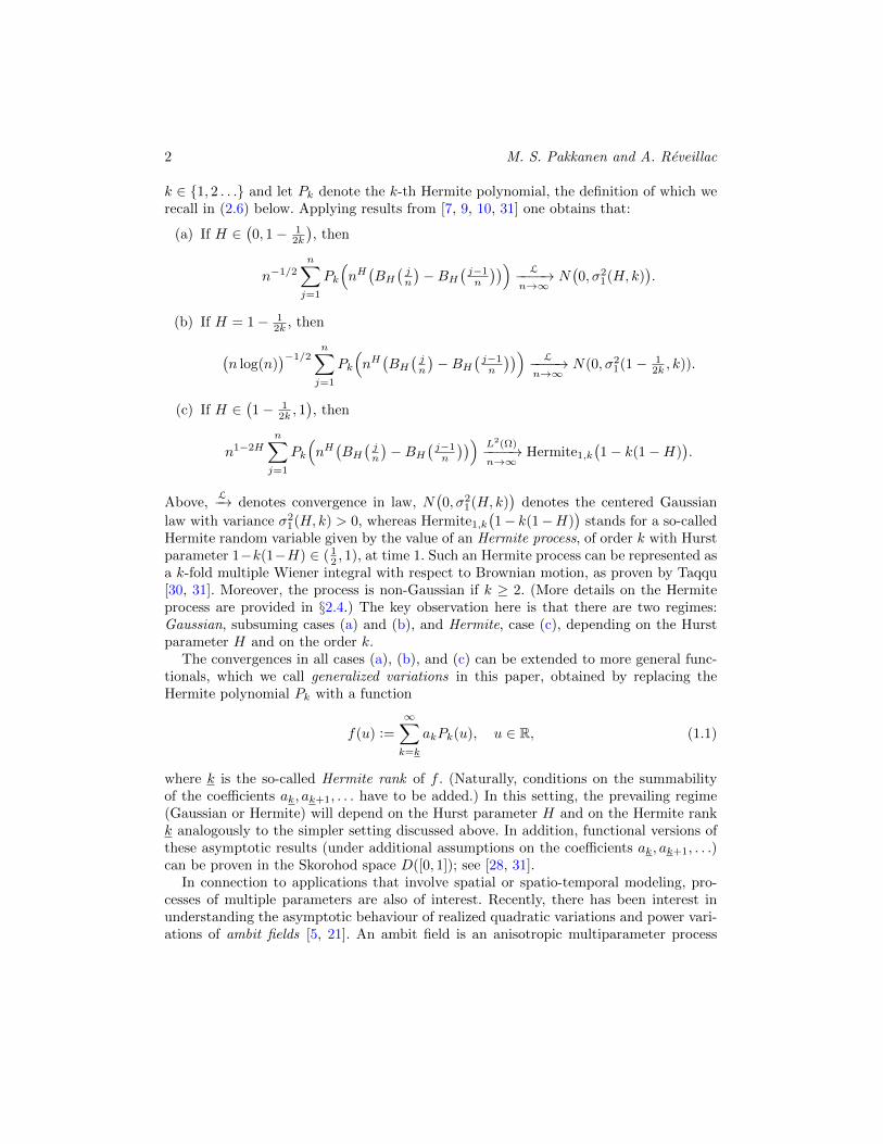
k ∈ 1, 2 . . . and let Pk denote the k-th Hermite polynomial, the definition of which werecall in (2.6) below. Applying results from [7, 9, 10, 31] one obtains that:

(a) If H ∈(0, 1− 1

2k

), then

n−1/2n∑j=1

Pk

(nH(BH(jn

)−BH

(j−1n

))) L−−−−→n→∞

N(0, σ2

1(H, k)).

(b) If H = 1− 12k , then

(n log(n)

)−1/2n∑j=1

Pk

(nH(BH(jn

)−BH

(j−1n

))) L−−−−→n→∞

N(0, σ21(1− 1

2k , k)).

(c) If H ∈(1− 1

2k , 1), then

n1−2Hn∑j=1

Pk

(nH(BH(jn

)−BH

(j−1n

))) L2(Ω)−−−−→n→∞

Hermite1,k

(1− k(1−H)

).

Above,L−→ denotes convergence in law, N

(0, σ2

1(H, k))

denotes the centered Gaussian

law with variance σ21(H, k) > 0, whereas Hermite1,k

(1− k(1−H)

)stands for a so-called

Hermite random variable given by the value of an Hermite process, of order k with Hurstparameter 1−k(1−H) ∈ ( 1

2 , 1), at time 1. Such an Hermite process can be represented asa k-fold multiple Wiener integral with respect to Brownian motion, as proven by Taqqu[30, 31]. Moreover, the process is non-Gaussian if k ≥ 2. (More details on the Hermiteprocess are provided in §2.4.) The key observation here is that there are two regimes:Gaussian, subsuming cases (a) and (b), and Hermite, case (c), depending on the Hurstparameter H and on the order k.

The convergences in all cases (a), (b), and (c) can be extended to more general func-tionals, which we call generalized variations in this paper, obtained by replacing theHermite polynomial Pk with a function

f(u) :=

∞∑k=k

akPk(u), u ∈ R, (1.1)

where k is the so-called Hermite rank of f . (Naturally, conditions on the summabilityof the coefficients ak, ak+1, . . . have to be added.) In this setting, the prevailing regime(Gaussian or Hermite) will depend on the Hurst parameter H and on the Hermite rankk analogously to the simpler setting discussed above. In addition, functional versions ofthese asymptotic results (under additional assumptions on the coefficients ak, ak+1, . . .)can be proven in the Skorohod space D([0, 1]); see [28, 31].

In connection to applications that involve spatial or spatio-temporal modeling, pro-cesses of multiple parameters are also of interest. Recently, there has been interest inunderstanding the asymptotic behaviour of realized quadratic variations and power vari-ations of ambit fields [5, 21]. An ambit field is an anisotropic multiparameter process

Limit theorems for the fractional Brownian sheet 3

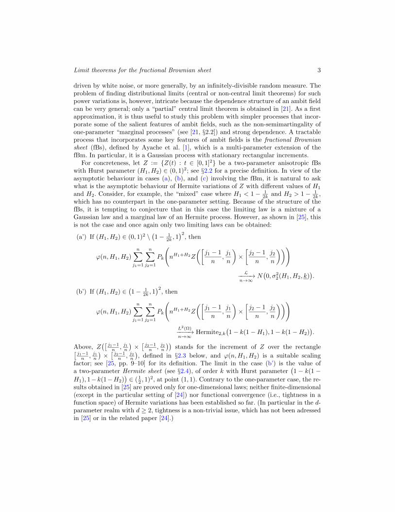
driven by white noise, or more generally, by an infinitely-divisible random measure. Theproblem of finding distributional limits (central or non-central limit theorems) for suchpower variations is, however, intricate because the dependence structure of an ambit fieldcan be very general; only a “partial” central limit theorem is obtained in [21]. As a firstapproximation, it is thus useful to study this problem with simpler processes that incor-porate some of the salient features of ambit fields, such as the non-semimartingality ofone-parameter “marginal processes” (see [21, §2.2]) and strong dependence. A tractableprocess that incorporates some key features of ambit fields is the fractional Browniansheet (fBs), defined by Ayache et al. [1], which is a multi-parameter extension of thefBm. In particular, it is a Gaussian process with stationary rectangular increments.

For concreteness, let Z := Z(t) : t ∈ [0, 1]2 be a two-parameter anisotropic fBswith Hurst parameter (H1, H2) ∈ (0, 1)2; see §2.2 for a precise definition. In view of theasymptotic behaviour in cases (a), (b), and (c) involving the fBm, it is natural to askwhat is the asymptotic behaviour of Hermite variations of Z with different values of H1

and H2. Consider, for example, the “mixed” case where H1 < 1− 12k and H2 > 1− 1

2k ,which has no counterpart in the one-parameter setting. Because of the structure of thefBs, it is tempting to conjecture that in this case the limiting law is a mixture of aGaussian law and a marginal law of an Hermite process. However, as shown in [25], thisis not the case and once again only two limiting laws can be obtained:

(a’) If (H1, H2) ∈ (0, 1)2 \(1− 1

2k , 1)2

, then

ϕ(n,H1, H2)

n∑j1=1

n∑j2=1

Pk

(nH1+H2Z

([j1 − 1

n,j1n

)×[j2 − 1

n,j2n

)))L−−−−→

n→∞N(0, σ2

2(H1, H2, k)).

(b’) If (H1, H2) ∈(1− 1

2k , 1)2

, then

ϕ(n,H1, H2)

n∑j1=1

n∑j2=1

Pk

(nH1+H2Z

([j1 − 1

n,j1n

)×[j2 − 1

n,j2n

)))L2(Ω)−−−−→n→∞

Hermite2,k

(1− k(1−H1), 1− k(1−H2)

).

Above, Z([j1−1n , j1n

)×[j2−1n , j2n

))stands for the increment of Z over the rectangle[

j1−1n , j1n

)×[j2−1n , j2n

), defined in §2.3 below, and ϕ(n,H1, H2) is a suitable scaling

factor; see [25, pp. 9–10] for its definition. The limit in the case (b’) is the value ofa two-parameter Hermite sheet (see §2.4), of order k with Hurst parameter

(1 − k(1 −

H1), 1−k(1−H2))∈ ( 1

2 , 1)2, at point (1, 1). Contrary to the one-parameter case, the re-sults obtained in [25] are proved only for one-dimensional laws; neither finite-dimensional(except in the particular setting of [24]) nor functional convergence (i.e., tightness in afunction space) of Hermite variations has been established so far. (In particular in the d-parameter realm with d ≥ 2, tightness is a non-trivial issue, which has not been adressedin [25] or in the related paper [24].)


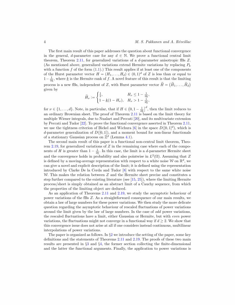
The first main result of this paper addresses the question about functional convergencein the general, d-parameter case for any d ∈ N. We prove a functional central limittheorem, Theorem 2.11, for generalized variations of a d-parameter anisotropic fBs Z.(As mentioned above, generalized variations extend Hermite variations by replacing Pkwith a function f of the form (1.1).) This result applies if at least one of the componentsof the Hurst parameter vector H = (H1, . . . ,Hd) ∈ (0, 1)d of Z is less than or equal to1− 1

2k , where k is the Hermite rank of f . A novel feature of this result is that the limiting

process is a new fBs, independent of Z, with Hurst parameter vector H =(H1, . . . , Hd

)given by

Hν :=

12 , Hν ≤ 1− 1

2k ,

1− k(1−Hν), Hν > 1− 12k ,

for ν ∈ 1, . . . , d. Note, in particular, that if H ∈(0, 1− 1

2k

]d, then the limit reduces to

an ordinary Brownian sheet. The proof of Theorem 2.11 is based on the limit theory formultiple Wiener integrals, due to Nualart and Peccati [20], and its multivariate extensionby Peccati and Tudor [22]. To prove the functional convergence asserted in Theorem 2.11,we use the tightness criterion of Bickel and Wichura [6] in the space D([0, 1]d), which isd-parameter generalization of D([0, 1]), and a moment bound for non-linear functionalsof a stationary Gaussian process on Zd (Lemma 4.1).

The second main result of this paper is a functional non-central limit theorem, Theo-rem 2.19, for generalized variations of Z in the remaining case where each of the compo-nents of H is greater than 1− 1

2k . In this case, the limit is a d-parameter Hermite sheet

and the convergence holds in probability and also pointwise in L2(Ω). Assuming that Zis defined by a moving-average representation with respect to a white noise W on Rd, wecan give a novel and explicit description of the limit; it is defined using the representationintroduced by Clarke De la Cerda and Tudor [8] with respect to the same white noiseW. This makes the relation between Z and the Hermite sheet precise and constitutes astep further compared to the existing literature (see [15, 25]), where the limiting Hermiteprocess/sheet is simply obtained as an abstract limit of a Cauchy sequence, from whichthe properties of the limiting object are deduced.

As an application of Theorems 2.11 and 2.19, we study the asymptotic behaviour ofpower variations of the fBs Z. As a straightforward consequence of our main results, weobtain a law of large numbers for these power variations. We then study the more delicatequestion regarding the asymptotic behaviour of rescaled fluctuations of power variationsaround the limit given by the law of large numbers. In the case of odd power variations,the rescaled fluctuations have a limit, either Gaussian or Hermite, but with even powervariations, the fluctuations might not converge in a functional way if d ≥ 2. We show thatthis convergence issue does not arise at all if one considers instead continuous, multilinearinterpolations of power variations.

The paper is organized as follows. In §2 we introduce the setting of the paper, some keydefinitions and the statements of Theorems 2.11 and 2.19. The proofs of these two mainresults are presented in §3 and §4, the former section collecting the finite-dimensionaland the latter the functional arguments. Finally, the application to power variations is


given in §5.

2. Preliminaries and main results

2.1. Notations

We use the convention that N := 1, 2, . . . and R+ := [0,∞). The notation |A| standsfor the cardinality of a finite set A. For any y ∈ R, we write byc := maxn ∈ Z : n ≤ v,y := y − byc, and (y)+ := max(y, 0). The symbol γ denotes the standard Gaussianmeasure on R, i.e., γ(dy) := (2π)−1/2 exp(−y2/2)dy. From now on we fix d in N.

For any vectors s = (s1, . . . , sd) ∈ Rd and t = (t1, . . . , td) ∈ Rd, the relation s ≤ t(resp. s < t) signifies that sν ≤ tν (resp. sν < tν) for all ν ∈ 1, . . . , d. We also use thenotation

st := (s1t1, . . . , sdtd) ∈ Rd,s

t:=(s1

t1, . . . ,

sdtd

)∈ Rd,

bsc := (bs1c, . . . , bsdc) ∈ Zd, 〈s〉 := s1 · · · sd ∈ R,|s| := (|s1|, . . . , |sd|) ∈ Rd+, s := (s1, . . . , sd) ∈ [0, 1)d.

Further, when s ∈ Rd+, we write st := (st11 , . . . , stdd ) ∈ Rd+, and when s ≤ t, we

write [s, t) := [s1, t1) × · · · × [sd, td) ⊂ Rd. Occasionally, we use the norm ‖s‖∞ :=max(|s1|, . . . , |sd|) for s ∈ Rd.

For the sake of clarity, we will consistently use the following convention: i, i(1), i(2), . . .are multi-indices (vectors) in Zd and j, j1, j2, . . . are indices (scalars) in Z.

2.2. Anisotropic fractional Brownian sheet

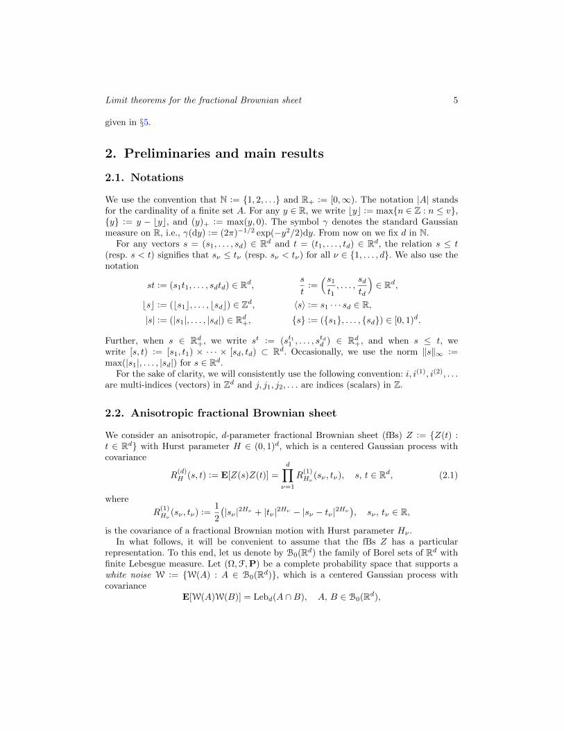
We consider an anisotropic, d-parameter fractional Brownian sheet (fBs) Z := Z(t) :t ∈ Rd with Hurst parameter H ∈ (0, 1)d, which is a centered Gaussian process withcovariance

R(d)H (s, t) := E[Z(s)Z(t)] =

d∏ν=1

R(1)Hν

(sν , tν), s, t ∈ Rd, (2.1)

where

R(1)Hν

(sν , tν) :=1

2

(|sν |2Hν + |tν |2Hν − |sν − tν |2Hν

), sν , tν ∈ R,

is the covariance of a fractional Brownian motion with Hurst parameter Hν .In what follows, it will be convenient to assume that the fBs Z has a particular

representation. To this end, let us denote by B0(Rd) the family of Borel sets of Rd withfinite Lebesgue measure. Let (Ω,F,P) be a complete probability space that supports awhite noise W := W(A) : A ∈ B0(Rd), which is a centered Gaussian process withcovariance

E[W(A)W(B)] = Lebd(A ∩B), A, B ∈ B0(Rd),


where Lebd(·) denotes the Lebesgue measure on Rd. The process Z can be defined as aWiener integral with respect to W (see, e.g., [19] for the definition), namely

Z(t) :=

∫G

(d)H (t, u)W(du), t ∈ Rd, (2.2)

where the kernel

G(d)H (t, u) :=

d∏ν=1

G(1)Hν

(tν , uν), t, u ∈ Rd, (2.3)

is defined using the one-dimensional Mandelbrot–Van Ness [13] kernel

G(1)Hν

(tν , uν) :=1

χ(Hν)

((tν − uν)

Hν− 12

+ − (−uν)Hν− 1

2+

), tν , uν ∈ R, (2.4)

with the normalizing constant

χ(Hν) :=

(1

2Hν+

∫ ∞0

((1 + y)Hν−

12 − yHν− 1

2

)dy

) 12

.

We refer to [1] for a proof that the process Z defined via (2.2) does indeed have thecovariance structure (2.1). The fBs admits a continuous modification (see [3, p. 1040]),so we may assume from now on that Z is continuous.

2.3. Increments and generalized variations

Given a function (or a realization of a stochastic process) h : Rd → R, we define theincrement of h over the half-open hyperrectangle [s, t) ⊂ Rd for any s ≤ t by

h([s, t)) :=∑

i∈0,1d(−1)d−

∑dν=1 iνh

((1− i)s+ it

).

(Note that iν above stands for the ν-th component of the multi-index i.) This definitioncan be recovered by differencing iteratively with respect to each of the arguments ofthe function h. Thus, the increment can be seen as a discrete analogue of the partial

derivative ∂d

∂t1···∂td .

Remark 2.5. It is useful to note that if there exists functions hν : R → R, ν ∈1, . . . , d, such that h(t) = h1(t1) · · ·hd(td) for any t ∈ Rd, then

h([s, t)) =

d∏ν=1

(hν(tν)− hν(sν)

),

which is easily verified by induction with respect to d using iterative differencing.


Let us fix a sequence(m(n)

)n∈N ⊂ Nd of multi-indices with the property

m(n) := min(m1(n), . . . ,md(n)

)−−−−→n→∞

∞

and a function f ∈ L2(R, γ) such that∫R f(u)γ(du) = 0. Our aim is to study the

asymptotic behaviour of a familyU

(n)f : n ∈ N

of d-parameter processes, generalized

variations of Z, defined by

U(n)f (t) :=

∑1≤i≤bm(n)tc

f

(⟨m(n)H

⟩Z

([i− 1

m(n),

i

m(n)

))), t ∈ [0, 1]d, n ∈ N.

In this definition,⟨m(n)H

⟩= m1(n)H1 · · ·md(n)Hd according to the notations and con-

ventions set forth in §2.1. The realizations of U(n)f belong to the space D([0, 1]d), which for

d ≥ 2 is a generalization of the space D([0, 1]) of cadlag functions on [0, 1]. We refer to [6,pp. 1662] for the definition of the space D([0, 1]d). In particular, C([0, 1]d) ⊂ D([0, 1]d).We endow D([0, 1]d) with the Skorohod topology described in [6, pp. 1662]. Convergenceto a continuous function in this topology is, however, equivalent to uniform convergence(see, e.g., [21, Lemma B.2] for a proof in the case d = 2).

2.4. Functional limit theorems for generalized variations

We will now formulate two functional limit theorems for the familyU

(n)f : n ∈ N

of

generalized variations, defined above. The class of admissible functions f needs to berestricted somewhat, however, and the choice of f and the Hurst parameter H of Z will

determine which of the limit theorems applies. Also, we need to rescale U(n)f in suitable

way that, likewise, depends on both f and H.To this end, recall that the Hermite polynomials,

P0(u) := 1, Pk(u) := (−1)keu2

2dk

duke−

u2

2 , u ∈ R, k ∈ N, (2.6)

form a complete orthogonal system in L2(R, γ). Thus, we may expand f in L2(R, γ) as

f(u) =

∞∑k=k

akPk(u), (2.7)

where the Hermite coefficients ak, ak+1, . . . ∈ R are such that ak 6= 0 and

∞∑k=k

k!a2k <∞. (2.8)

The index k is called the Hermite rank of f , and the proviso∫R f(u)γ(du) = 0 ensures

that k ≥ 1. We will assume that the Hermite coefficients decay somewhat faster thanwhat (2.8) entails.


Assumption 2.9. The Hermite coefficients ak, ak+1, . . . of the function f satisfy

∞∑k=k

3k2

√k!|ak| <∞.

Let us define a sequence(c(n)

)n∈N ⊂ Rd+ of rescaling factors by setting for any ν ∈

1, . . . , d and n ∈ N,

cν(n) :=

mν(n)2−2k(1−Hν), Hν ∈

(1− 1

2k , 1),

mν(n) log(mν(n)

), Hν = 1− 1

2k ,

mν(n), Hν ∈(0, 1− 1

2k

).

Remark 2.10. Note that lim supn→∞mν(n)cν(n) <∞ and that, in fact, limn→∞

mν(n)cν(n) = 0

if Hν ∈[1− 1

2k , 1).

Now we can define a familyU

(n)

f : n ∈ N of rescaled generalized variations as

U(n)

f (t) :=U

(n)f (t)

〈c(n)〉 12

, t ∈ [0, 1]d, n ∈ N.

Our first result is the following functional central limit theorem (FCLT) for generalizedvariations. Its proof is carried out in §3.2 and §4.2.

Theorem 2.11 (FCLT). Let f be as above such that Assumption 2.9 holds and suppose

that H ∈ (0, 1)d \(1− 1

2k , 1)d

. Then

(Z, U

(n)

f

) L−−−−→n→∞

(Z, Λ

12

H,f Z)

in D([0, 1]d)2, (2.12)

where Z is a d-parameter fBs with Hurst parameter H ∈[

12 , 1)d

, independent of Z(defined, possibly, on an extension of (Ω,F,P)), and

ΛH,f :=

∞∑k=max(k,2)

k!a2k〈b(k)〉 ∈ R. (2.13)

The vectors H ∈[

12 , 1)d

and b(k) ∈ Rd+, k ≥ max(k, 2), that appear above are defined bysetting for any ν ∈ 1, . . . , d,

Hν :=

12 , Hν ∈

(0, 1− 1

2k

],

1− k(1−Hν), Hν ∈(1− 1

2k , 1),

(2.14)


and

b(k)ν :=

∑j∈Z

(|j + 1|2Hν − 2|j|2Hν + |j − 1|2Hν

2

)k, Hν ∈

(0, 1− 1

2k

),

2

((2k − 1)(k − 1)

2k2

)k=: ι(k), Hν = 1− 1

2k , k = k,

Hkν (2Hν − 1)k

(1− k(1−Hν))(1− 2k(1−Hν))=: κ(Hν , k), Hν ∈

(1− 1

2k , 1), k = k,

0, Hν ∈[1− 1

2k , 1), k > k.

(2.15)

Remark 2.16. (1) The counterpart of the convergence (2.12) for finite dimensionallaws holds without Assumption 2.9, see Proposition 3.15, below.

(2) We may use max(k, 2), instead of k, as the lower bound for the summation index kin (2.13) since ι(1) = 0 and

∑j∈Z

|j + 1|2H − 2|j|2H + |j − 1|2H

2

=∑j∈Z

|j|2H − |j − 1|2H

2−∑j∈Z

|j|2H − |j − 1|2H

2= 0

for any H ∈(0, 1

2

). (Then,

∑j∈Z

∣∣ |j|2H−|j−1|2H2

∣∣ <∞ by the mean value theorem.)(3) The convergence (2.12) can be understood in the framework of stable convergence

in law, introduced by Renyi [23]. Equivalently to (2.12), U(n)

f converges to Λ12

H,f Z as

n→∞ stably in law with respect to the σ-algebra generated by Z(t) : t ∈ [0, 1]d.

Theorem 2.11 excludes the case H ∈(1− 1

2k , 1)d

. Then, the generalized variations do

have a limit, but the limit is non-Gaussian, unless k = 1. To describe the limit, we needthe following definition, due to Clarke De la Cerda and Tudor [8].

Definition 2.17. An anisotropic, d-parameter Hermite sheet Z :=Z(t) : t ∈ Rd+

of order k ≥ 2 with Hurst parameter H ∈

(12 , 1)d

is defined as a k-fold multiple Wienerintegral (see §3.2) with respect to the white noise W,

Z(t) :=

∫· · ·∫G

(k)

H

(t, u(1), . . . , u(k)

)W(du(1)

)· · ·W

(du(k)

):= IWk

(G

(k)

H

(t, ·))

(2.18)


for any t ∈ Rd+. In (2.18), the kernel G(d,k)

H(t, ·) ∈ L2(Rkd) is given by

G(k)

H

(t, u(1), . . . , u(k)

):=

1

χ(H, k

) ∫[0,t)

k∏κ=1

d∏ν=1

(yν − u(κ)

ν

)− 12−

1−Hνk

+dy, u(1), . . . , u(k) ∈ Rd,

using the normalizing constant

χ(H, k

):=

d∏ν=1

(B(

12 −

1−Hνk , 2(Hν−1)

k

)Hν(2Hν − 1)

) 12

,

where B stands for the beta function.

The Hermite sheet Z is self-similar and has the same correlation structure as a fBs withHurst parameter H. In the case k = 1, the process Z is Gaussian (in fact, it coincides with

a fractional Brownian sheet with Hurst parameter H) but for k ≥ 2 it is non-Gaussian. Inthe case k = 2, the name Rosenblatt sheet (and Rosenblatt process, when d = 1; see [32])is often used, in honor of Murray Rosenblatt’s seminal paper [26]. See also the recentpapers [12, 33] for more details on the Rosenblatt distribution, including proofs that thisdistribution is infinitely divisible.

As our second main result, we obtain the following functional non-central limit theorem(FNCLT) for generalized variations. The proof of this result is carried out in §3.3 and§4.2.

Theorem 2.19 (FNCLT). Let f be as above such that Assumption 2.9 holds and sup-

pose that H ∈(1− 1

2k , 1)d

. Then,

U(n)

fP−−−−→

n→∞Λ

12

H,f Z in D([0, 1]d), (2.20)

where Z is a d-parameter Hermite sheet of order k with Hurst parameter H, given by(2.14), and ΛH,f is given by (2.13).

Remark 2.21. (1) The convergence (2.20) holds pointwise in L2(Ω,F,P), even whenAssumption 2.9 does not hold, see Proposition 3.27, below.

(2) Unlike in Theorem 2.11, the non-central limit Z is defined on the original probability

space (Ω,F,P). In particular, Z is driven by the same white noise W as Z.(3) In the special case k = 1, the limit in (2.20) is Gaussian. In fact, then ΛH,f = a2

1

and Z = Z.

Remark 2.22. Our method of proving the convergence of finite-dimensional distribu-

tions of U(n)

f , using chaotic expansions, is particularly suitable for providing estimates


on the speed of convergence (for example in the Wasserstein distance) as is done in [18]following the original idea presented in [16], which combines the Malliavin calculus andStein’s method. In addition, the study of weighted variations of the fBs is still partially in-complete, especially with regards to functional convergence (see [24]). To keep the lengthof this paper within limits — and since proving functional convergence of weighted vari-ations requires slighly different methods — we have decided to treat these two questionsin a separate paper.

3. Finite-dimensional convergence

In this section, we begin the proofs of Theorems 2.11 and 2.19. To be more precise, weprove the finite-dimensional statements corresponding to (2.12) and (2.20), see Proposi-tions 3.15 and 3.27, respectively. As a preparation, we study the correlation structure ofthe increments of the fBs Z and recall the chaotic expansion of functionals of Z.

3.1. Correlation structure of increments

In what follows, it will be convenient to use the shorthand

Z(n)i := 〈m(n)H〉Z

([i− 1

m(n),

i

m(n)

)), 1 ≤ i ≤ m(n), n ∈ N. (3.1)

For any n ∈ N, the familyZ

(n)i : 1 ≤ i ≤ m(n)

is clearly centered and Gaussian. We

will next derive its correlation structure.To describe the correlation structure of the rescaled increments (3.1), let BH(t) : t ∈

R be an auxiliary fractional Brownian motion with Hurst parameter H ∈ (0, 1). Usingthe kernel (2.4), we may represent it as

BH(t) :=

∫RG

(1)

H(t, u)dB(u), t ∈ R,

where B(t) : t ∈ R is a standard Brownian motion. Recall that BH is H-self similar,i.e.,

BH(at) : t ∈ R L

=aHBH(t) : t ∈ R

for any a > 0, (3.2)

and has stationary increments, i.e.,BH([s, s+ t)) : t ∈ R

L= BH([0, t)) : t ∈ R for any s ∈ R. (3.3)

The discrete parameter process

BH([j, j + 1)), j ∈ Z,


which is stationary by (3.3), is called a fractional Gaussian noise. Its correlation functioncan be expressed as

rH(j) := E[BH([j, j + 1))BH([0, 1))

]=|j + 1|2H − 2|j|2H + |j − 1|2H

2, j ∈ Z.

One can show, e.g., using the mean value theorem, that there exists a constant C(H) > 0such that

|rH(j)| ≤ C(H)|j|−2(1−H), j ∈ Z. (3.4)

Thus, if k > 12 and H ∈

(0, 1− 1

2k

), then∑j∈Z|rH(j)|k <∞. (3.5)

If H ∈[1 − 1

2k , 1), then the series (3.5) diverges. In this case it is still useful to have

estimates for the partial sums corresponding to (3.5). Using (3.4), one can prove thatthere exists a constant C ′(H, k) > 0 such that∑

|j|<l

|rH(j)|k ≤

C ′(H, k) log l, H = 1− 1

2k ,

C ′(H, k)l1−2k(1−H), H ∈(1− 1

2k , 1).

(3.6)

We can now describe the correlations of the rescaled increments (3.1) using the corre-lation function of the fractional Gaussian noise as follows.

Lemma 3.7 (Correlation structure). For any n ∈ N, and 1 ≤ i(1), i(2) ≤ m(n),

E[Z

(n)

i(1)Z(n)

i(2)

]=

d∏ν=1

rHν(i(1)ν − i(2)

ν

).

Proof. Using first the linearity of Wiener integrals and then the product structure (2.3)

of the kernel G(d)H and Remark 2.5, we obtain for any s, t ∈ [0, 1]d such that s ≤ t,

Z([s, t)) =

∫G

(d)H ([s, t), u)W(du) =

∫ d∏ν=1

G(1)Hν

([sν , tν), uν)W(du). (3.8)

Thus, by Fubini’s theorem,

E

[Z

([i(1) − 1

m(n),i(1)

m(n)

))Z

([i(2) − 1

m(n),i(2)

m(n)

))]

=

d∏ν=1

∫G

(1)Hν

([i(1)ν − 1

mν(n),i(1)ν

mν(n)

), v

)G

(1)Hν

([i(2)ν − 1

mν(n),i(2)ν

mν(n)

), v

)dv

=

d∏ν=1

E

[BHν

([i(1)ν − 1

mν(n),i(1)ν

mν(n)

))BHν

([i(2)ν − 1

mν(n),i(2)ν

mν(n)

))].


For any ν ∈ 1, . . . , d, the fractional Brownian motion BHν is Hν-self similar and hasstationary increments, cf. (3.2) and (3.3), so we obtain

E

[BHν

([i(1)ν − 1

mν(n),i(1)ν

mν(n)

))BHν

([i(2)ν − 1

mν(n),i(2)ν

mν(n)

))]=rHν

(i(1)ν − i(2)

ν

)mν(n)2Hν

,

from which the assertion follows.

3.2. Multiple Wiener integrals and central limit theorem

The proofs of Theorems 2.11 and 2.19 rely on particular representations of generalizedvariations in terms of multiple Wiener integrals with respect to the underlying whitenoise W. We will now briefly review the theory of multiple Wiener integrals and howthese integrals can be used to prove central limit theorems. As an application, we takethe first step in the proof of Theorem 2.11 by establishing the convergence of finite-dimensional laws.

In what follows, we write H := L2(Rd). Recall that H is a separable Hilbert spacewhen we endow it with the usual inner product. For any k ∈ N, we denote by H⊗k thek-fold tensor power of H and by Hk ⊂ H⊗k the symmetrization of H⊗k. Note that wecan make the identification H⊗k ∼= L2(Rkd). For any h ∈ Hk, we may define the k-foldmultiple Wiener integral IWk (h) of h with respect to W. This is done, using Hermitepolynomials, by setting for any κ ∈ N, any orthonormal h1, . . . , hκ ∈ H, and for anyk1, . . . , kκ ∈ N such that k1 + · · ·+ kκ = k,

IWk

(κ⊙j=1

h⊗kjj

):= k!

κ∏j=1

Pkj

(∫hj(u)W(du)

), (3.9)

where denotes symmetrization of the tensor product, and extended to general inte-grands h ∈ Hk using a density argument. It is worth stressing that the multiple Wienerintegral is linear with respect to the integrand and has zero expectation. Moreover, by(3.9), for h ∈ H one has

IW1 (h) =

∫h(u)W(du), (3.10)

and if ‖h‖H = 1, then for any k ∈ N it holds that h⊗k ∈ Hk and

Pk(IW1 (h)

)= IWk (h⊗k). (3.11)

Multiple Wiener integrals have the following isometry and orthogonality properties: forany k1, k2 ∈ N, h1 ∈ Hk1 , and h2 ∈ Hk2 ,

E[IWk1

(h1)IWk2(h2)

]=

k1!〈h1, h2〉H⊗k1 , k1 = k2,

0, k1 6= k2.(3.12)


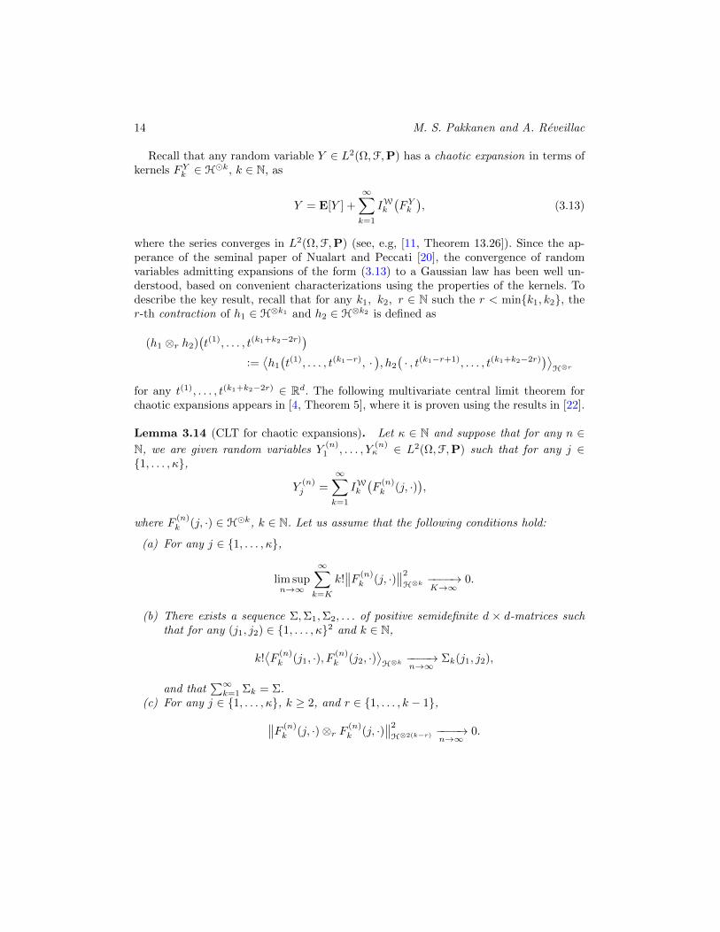
Recall that any random variable Y ∈ L2(Ω,F,P) has a chaotic expansion in terms ofkernels FYk ∈ Hk, k ∈ N, as

Y = E[Y ] +

∞∑k=1

IWk(FYk), (3.13)

where the series converges in L2(Ω,F,P) (see, e.g, [11, Theorem 13.26]). Since the ap-perance of the seminal paper of Nualart and Peccati [20], the convergence of randomvariables admitting expansions of the form (3.13) to a Gaussian law has been well un-derstood, based on convenient characterizations using the properties of the kernels. Todescribe the key result, recall that for any k1, k2, r ∈ N such the r < mink1, k2, ther-th contraction of h1 ∈ H⊗k1 and h2 ∈ H⊗k2 is defined as

(h1 ⊗r h2)(t(1), . . . , t(k1+k2−2r)

):=⟨h1

(t(1), . . . , t(k1−r), ·

), h2

(· , t(k1−r+1), . . . , t(k1+k2−2r)

)⟩H⊗r

for any t(1), . . . , t(k1+k2−2r) ∈ Rd. The following multivariate central limit theorem forchaotic expansions appears in [4, Theorem 5], where it is proven using the results in [22].

Lemma 3.14 (CLT for chaotic expansions). Let κ ∈ N and suppose that for any n ∈N, we are given random variables Y

(n)1 , . . . , Y

(n)κ ∈ L2(Ω,F,P) such that for any j ∈

1, . . . , κ,

Y(n)j =

∞∑k=1

IWk(F

(n)k (j, ·)

),

where F(n)k (j, ·) ∈ Hk, k ∈ N. Let us assume that the following conditions hold:

(a) For any j ∈ 1, . . . , κ,

lim supn→∞

∞∑k=K

k!∥∥F (n)

k (j, ·)∥∥2

H⊗k−−−−→K→∞

0.

(b) There exists a sequence Σ,Σ1,Σ2, . . . of positive semidefinite d × d-matrices suchthat for any (j1, j2) ∈ 1, . . . , κ2 and k ∈ N,

k!⟨F

(n)k (j1, ·), F (n)

k (j2, ·)⟩H⊗k

−−−−→n→∞

Σk(j1, j2),

and that∑∞k=1 Σk = Σ.

(c) For any j ∈ 1, . . . , κ, k ≥ 2, and r ∈ 1, . . . , k − 1,∥∥F (n)k (j, ·)⊗r F (n)

k (j, ·)∥∥2

H⊗2(k−r) −−−−→n→∞

0.


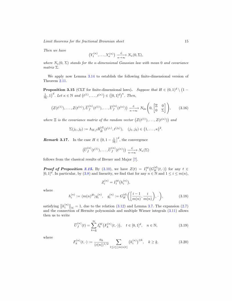
Then we have (Y

(n)1 , . . . , Y (n)

κ

) L−−−−→n→∞

Nκ(0,Σ),

where Nκ(0, Σ) stands for the κ-dimensional Gaussian law with mean 0 and covariancematrix Σ.

We apply now Lemma 3.14 to establish the following finite-dimensional version ofTheorem 2.11.

Proposition 3.15 (CLT for finite-dimensional laws). Suppose that H ∈ (0, 1)d \(1 −

12k , 1

)d. Let κ ∈ N and

(t(1), . . . , t(κ)

)∈([0, 1]d

)κ. Then,

(Z(t(1)), . . . , Z(t(κ)), U

(n)

f (t(1)), . . . , U(n)

f (t(κ))) L−−−−→n→∞

N2κ

(0,

[Ξ 00 Σ

]), (3.16)

where Ξ is the covariance matrix of the random vector(Z(t(1)), . . . , Z(t(κ))

)and

Σ(j1, j2) := ΛH,fR(d)

H(t(j1), t(j2)), (j1, j2) ∈ 1, . . . , κ2.

Remark 3.17. In the case H ∈(0, 1− 1

2k

]d, the convergence

(U

(n)

f (t(1)), . . . , U(n)

f (t(κ))) L−−−−→n→∞

Nκ(Σ)

follows from the classical results of Breuer and Major [7].

Proof of Proposition 3.15. By (3.10), we have Z(t) = IW1(G

(d)H (t, ·)

)for any t ∈

[0, 1]d. In particular, by (3.8) and linearity, we find that for any n ∈ N and 1 ≤ i ≤ m(n),

Z(n)i = IW1

(h

(n)i

),

where

h(n)i := 〈m(n)H〉g(n)

i , g(n)i := G

(d)H

([i− 1

m(n),

i

m(n)

), ·), (3.18)

satisfying∥∥h(n)

i

∥∥H

= 1, due to the relation (3.12) and Lemma 3.7. The expansion (2.7)and the connection of Hermite polynomials and multiple Wiener integrals (3.11) allowsthen us to write

U(n)

f (t) =

∞∑k=k

IWk(F

(n)k (t, ·)

), t ∈ [0, 1]d, n ∈ N, (3.19)

whereF

(n)k (t, ·) :=

ak〈c(n)〉1/2

∑1≤i≤bm(n)tc

(h

(n)i

)⊗k, k ≥ k. (3.20)


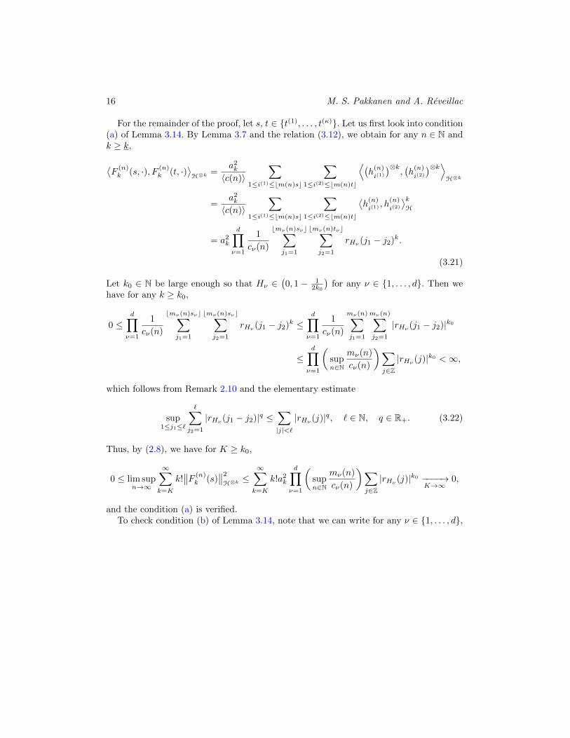
For the remainder of the proof, let s, t ∈ t(1), . . . , t(κ). Let us first look into condition(a) of Lemma 3.14. By Lemma 3.7 and the relation (3.12), we obtain for any n ∈ N andk ≥ k,

⟨F

(n)k (s, ·), F (n)

k (t, ·)⟩H⊗k

=a2k

〈c(n)〉∑

1≤i(1)≤bm(n)sc

∑1≤i(2)≤bm(n)tc

⟨(h

(n)

i(1)

)⊗k,(h

(n)

i(2)

)⊗k⟩H⊗k

=a2k

〈c(n)〉∑

1≤i(1)≤bm(n)sc

∑1≤i(2)≤bm(n)tc

⟨h

(n)

i(1) , h(n)

i(2)

⟩kH

= a2k

d∏ν=1

1

cν(n)

bmν(n)sνc∑j1=1

bmν(n)tνc∑j2=1

rHν (j1 − j2)k.

(3.21)

Let k0 ∈ N be large enough so that Hν ∈(0, 1 − 1

2k0

)for any ν ∈ 1, . . . , d. Then we

have for any k ≥ k0,

0 ≤d∏ν=1

1

cν(n)

bmν(n)sνc∑j1=1

bmν(n)sνc∑j2=1

rHν (j1 − j2)k ≤d∏ν=1

1

cν(n)

mν(n)∑j1=1

mν(n)∑j2=1

|rHν (j1 − j2)|k0

≤d∏ν=1

(supn∈N

mν(n)

cν(n)

)∑j∈Z|rHν (j)|k0 <∞,

which follows from Remark 2.10 and the elementary estimate

sup1≤j1≤`

∑j2=1

|rHν (j1 − j2)|q ≤∑|j|<`

|rHν (j)|q, ` ∈ N, q ∈ R+. (3.22)

Thus, by (2.8), we have for K ≥ k0,

0 ≤ lim supn→∞

∞∑k=K

k!∥∥F (n)

k (s)∥∥2

H⊗k≤∞∑k=K

k!a2k

d∏ν=1

(supn∈N

mν(n)

cν(n)

)∑j∈Z|rHν (j)|k0 −−−−→

K→∞0,

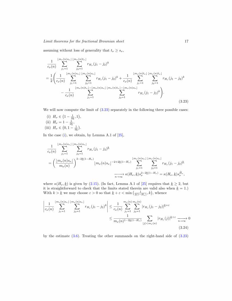
and the condition (a) is verified.To check condition (b) of Lemma 3.14, note that we can write for any ν ∈ 1, . . . , d,


assuming without loss of generality that tν ≥ sν ,

1

cν(n)

bmν(n)sνc∑j1=1

bmν(n)tνc∑j2=1

rHν (j1 − j2)k

=1

2

(1

cν(n)

bmν(n)sνc∑j1=1

bmν(n)sνc∑j2=1

rHν (j1 − j2)k +1

cν(n)

bmν(n)tνc∑j1=1

bmν(n)tνc∑j2=1

rHν (j1 − j2)k

− 1

cν(n)

bmν(n)tνc−bmν(n)sνc∑j1=1

bmν(n)tνc−bmν(n)sνc∑j2=1

rHν (j1 − j2)k

).

(3.23)

We will now compute the limit of (3.23) separately in the following three possible cases:

(i) Hν ∈(1− 1

2k , 1),

(ii) Hν = 1− 12k ,

(iii) Hν ∈(0, 1− 1

2k

).

In the case (i), we obtain, by Lemma A.1 of [25],

1

cν(n)

bmν(n)sνc∑j1=1

bmν(n)sνc∑j2=1

rHν (j1 − j2)k

=

(bmν(n)sνcmν(n)

)2−2k(1−Hν)

bmν(n)sνc−2+2k(1−Hν)

bmν(n)sνc∑j1=1

bmν(n)sνc∑j2=1

rHν (j1 − j2)k

−−−−→n→∞

κ(Hν , k)s2−2k(1−Hν)ν = κ(Hν , k)sHνν ,

where κ(Hν , k) is given by (2.15). (In fact, Lemma A.1 of [25] requires that k ≥ 2, butit is straightforward to check that the limits stated therein are valid also when k = 1.)With k > k we may choose ε > 0 so that k + ε < min

(1

2(1−Hν) , k), whence∣∣∣∣∣ 1

cν(n)

bmν(n)sνc∑j1=1

bmν(n)sνc∑j2=1

rHν (j1 − j2)k

∣∣∣∣∣ ≤ 1

cν(n)

mν(n)∑j1=1

mν(n)∑j2=1

|rHν (j1 − j2)|k+ε

≤ 1

mν(n)1−2k(1−Hν)

∑|j|<mν(n)

|rHν (j)|k+ε −−−−→n→∞

0

(3.24)

by the estimate (3.6). Treating the other summands on the right-hand side of (3.23)


similarly, we arrive at

limn→∞

1

cν(n)

bmν(n)sνc∑j1=1

bmν(n)tνc∑j2=1

rHν (j1 − j2)k

=

κ(Hν ,k)

2

(sHνν + tHνν − (tν − sν)Hν

)= κ(Hν , k)R

(1)

Hν(sν , tν), k = k,

0, k > k.

In the case (ii), rearranging and applying Lemma A.1 of [25] yields

1

cν(n)

bmν(n)sνc∑j1=1

bmν(n)sνc∑j2=1

rHν (j1 − j2)k

=

(1 +

log( bmν(n)sνc

mν(n)

)log(mν(n)

) )bmν(n)sνc/mν(n)

bmν(n)sνc log(bmν(n)sνc)

bmν(n)sνc∑j1=1

bmν(n)sνc∑j2=1

rHν (j1 − j2)k

−−−−→n→∞

ι(k)sν ,

where ι(k) is given by (2.15). When k > k, we have Hν ∈(0, 1− 1

2k

)and, consequently,∣∣∣∣∣ 1

cν(n)

bmν(n)sνc∑j1=1

bmν(n)sνc∑j2=1

rHν (j1 − j2)k

∣∣∣∣∣ ≤ 1

log(mν(n)

) ∑j∈Z|rHν (j)|k −−−−→

n→∞0.

Again, a similar treatment of the other summands on right-hand side of (3.23) establishesthat

limn→∞

1

cν(n)

bmν(n)sνc∑j1=1

bmν(n)tνc∑j2=1

rHν (j1 − j2)k

=

ι(k)

2

(sν + tν − (tν − sν)

)= ι(k)R

(1)

Hν(sν , tν), k = k,

0, k > k.

Finally, in the case (iii), we deduce in a straightforward manner that for any k ≥ k,

limn→∞

1

cν(n)

bmν(n)sνc∑j1=1

bmν(n)tνc∑j2=1

rHν (j1 − j2)k =1

2

∑j∈Z

rHν (j)k(sν + tν − (tν − sν)

)=∑j∈Z

rHν (j)kR(1)

Hν(sν , tν)

using Lemma A.1 of [25].Returning to the expression (3.21), we have shown that for any k ≥ k,

k!⟨F

(n)k (s), F

(n)k (t)

⟩H⊗k

−−−−→n→∞

k!a2k〈b(k)〉R(d)

H(s, t). (3.25)


When k = 1, we need to check, additionally, that the covariance matrix appearing inthe limit (3.16) is block-diagonal. To this end, note that it follows from the assumption

H ∈ (0, 1)d \(

12 , 1)d

, that b(1)ν = 0 for some ν ∈ 1, . . . , d, which in turn implies that∥∥F (n)

1 (s, ·)∥∥2

H−−−−→n→∞

0.

By the Cauchy–Schwarz inequality, we have then⟨F

(n)1 (s, ·), G(d)

H (t, ·)⟩H−−−−→n→∞

0,

which ensures block diagonality, and concludes the verification of condition (b).In order to check condition (c) of Lemma 3.14, let k ≥ max(k, 2) and r ∈ 1, . . . , k−1.

Using the bilinearity of contractions and inner products, we obtain∥∥F (n)k (t, ·)⊗r F (n)

k (t, ·)∥∥2

H⊗2(k−r)

=a4k

〈c(n)〉2∑

1≤i(j)≤bm(n)tcj∈1,2,3,4

⟨(h

(n)

i(1)

)⊗k ⊗r (h(n)

i(2)

)⊗k,(h

(n)

i(3)

)⊗k ⊗r (h(n)

i(4)

)⊗k⟩H⊗2(k−r)

=a4k

〈c(n)〉2∑

1≤i(j)≤bm(n)tcj∈1,2,3,4

⟨h

(n)

i(1) , h(n)

i(2)

⟩rH

⟨h

(n)

i(3) , h(n)

i(4)

⟩rH

⟨h

(n)

i(1) , h(n)

i(3)

⟩k−rH

⟨h

(n)

i(2) , h(n)

i(4)

⟩k−rH

= a4k

d∏ν=1

1

cν(n)2

bmν(n)tνc∑j1,j2,j3,j4=1

rHν (j1 − j2)rrHν (j3 − j4)rrHν (j1 − j3)k−rrHν (j2 − j4)k−r.

Following the proof of Lemma 4.1 of [17], we apply the bound

|rHν (j1)|r|rHν (j2)|k−r ≤ |rHν (j1)|k + |rHν (j2)|k, j1, j2 ∈ Z,

which is a consequence of Young’s inequality, and use repeatedly (3.22) to deduce that

∥∥F (n)k (t, ·)⊗r F (n)

k (t, ·)∥∥2

H⊗2(k−r) ≤ 16da4k

d∏ν=1

mν(n)φν(n)

cν(n)2, (3.26)

where

φν(n) :=∑

|j1|<mν(n)

|rHν (j1)|r∑

|j2|<mν(n)

|rHν (j2)|k−r∑

|j3|<mν(n)

|rHν (j3)|k.

We need to analyze the asymptotic behaviour of φν(n) as n → ∞. This can be ac-complished by considering separately the three possible cases:

(i’) Hν ∈(1− 1

2k , 1),


(ii’) Hν = 1− 12k ,

(iii’) Hν ∈(0, 1− 1

2k

).

In the case (i’) we have clearly Hν ∈(1 − 1

2(k−r) , 1)∩(1 − 1

2r , 1), and by the estimate

(3.6), it follows thatφν(n) ≤ C ′′(Hν , k, r)mν(n)3−4k(1−Hν),

where C ′′(Hν , k, r) := C ′(Hν , r)C′(Hν , k − r)C ′(Hν , k). Since Hν ∈

(1 − 1

2k , 1)⊂(1 −

12k , 1

), we obtain

lim supn→∞

mν(n)φν(n)

cν(n)2≤ lim sup

n→∞

C ′′(Hν , k, r)

mν(n)4(k−k)(1−Hν)<∞.

Let us then consider to the case (ii’). We have still Hν ∈(1− 1

2(k−r) , 1)∩(1− 1

2r , 1), so

by (3.6) we find that

φν(n) ≤ C ′′(Hν , k, r)mν(n)2−2k(1−Hν) log(mν(n)

)= C ′′(Hν , k, r)mν(n) log

(mν(n)

).

Necessarily Hν ∈[1 − 1

2k , 1), whence there is an index n0 ∈ N such that cν(n) ≥

mν(n) log(mν(n)

)for all n ≥ n0. We deduce then that

limn→∞

mν(n)φν(n)

cν(n)2≤ limn→∞

C ′′(Hν , k, r)

log(mν(n)

) = 0.

In the remaining case (iii’) we have∑j∈Z |rHν (j)|k <∞. Since there is n0 ∈ N such that

cν(n) ≥ mν(n) for all n ≥ n0, we find that

limn→∞

mν(n)φν(n)

cν(n)2

≤ limn→∞

1

mν(n)

∑|j1|<mν(n)

|rHν (j1)|r∑

|j2|<mν(n)

|rHν (j2)|k−r∑j3∈Z|rHν (j3)|k = 0

by Lemma 2.2 of [17].Finally, let us return to the upper bound (3.26). The crucial observation is that the

assumption H ∈ (0, 1)d \(1 − 1

2k , 1)d

implies that there is at least one coordinate ν ∈1, . . . , d that falls within case (ii’) or (iii’). Thus,∥∥F (n)

k (t, ·)⊗r F (n)k (t, ·)

∥∥2

H⊗2(k−r) −−−−→n→∞

0,

concluding the verification of the condition (c), and the convergence (3.16) follows.


3.3. Convergence to the Hermite sheet

We prove next a pointwise version of Theorem 2.19 in L2(Ω). The argument is basedmainly on the chaotic expansion (3.19) and the isometry property (3.12) of multipleWiener integrals. However, compared to the proof of Proposition 3.15, we need to analyzethe asymptotic behaviour of the associated kernels more carefully.

Proposition 3.27 (Pointwise NCLT). Suppose that H ∈(1 − 1

2k , 1)d

. Then, for any

t ∈ [0, 1]d,

U(n)

f (t)L2(Ω)−−−−→n→∞

Λ12

H,f Z(t), (3.28)

where Z is the Hermite sheet appearing in Theorem 2.19.

Proof. Fix t ∈ [0, 1]d. By the chaotic expansion (3.19), we have for any n ∈ N,

U(n)

f (t) = IWk(F

(n)k (t, ·)

)+

∞∑k=k+1

IWk(F

(n)k (t, ·)

).

Using the property (3.12) and Parseval’s identity, we find that

E

[( ∞∑k=k+1

IWk(F

(n)k (t, ·)

))2]=

∞∑k=k+1

k!∥∥F (n)

k (t, ·)∥∥2

H⊗k.

Since H ∈(1− 1

2k , 1)d

, we may choose ε ∈ (0, 1] so that H ∈(1− 1

2(k+ε) , 1)d

. Combining

(3.21) and (3.24), we find that

∞∑k=k+1

k!∥∥F (n)

k (t, ·)∥∥2

H⊗k≤

∞∑k=k+1

k!a2k

d∏ν=1

1


∑|j|<mν(n)

|rHν (j)|k+ε −−−−→n→∞

0,

where convergence to zero is a consequence of the bound (3.6). Thus, it remains to showthat

IWk(F

(n)k (t, ·)

) L2(Ω)−−−−→n→∞

IWk

(Λ

12

H,f G(k)

H(t, ·)

)= Λ

12

H,f Z(t),

which follows by (3.12), if we can show that

F(n)k (t, ·) H⊗k−−−−→

n→∞Λ

12

H,f G(k)

H(t, ·). (3.29)

In the special case k = 1, the convergence (3.28) follows already. Namely,

IW1(F

(n)1 (t, ·)

)= a1Z

(bm(n)tcm(n)

)L2(Ω)−−−−→n→∞

a1Z(t) = Λ12

H,fZ(t) = Λ12

H,f Z(t)

by the L2-continuity of Z. Thus, we can assume that k ≥ 2 from now on.


We will prove the convergence (3.29) in two steps. First, we show that(F

(n)k (t, ·)

)n∈N

is a Cauchy sequence in H⊗k. Later, we characterize the limit. Let n1, n2 ∈ N andconsider∥∥F (n1)

k (t, ·)− F (n2)k (t, ·)

∥∥2

H⊗k

=∥∥F (n1)

k (t, ·)∥∥2

H⊗k+∥∥F (n2)

k (t, ·)∥∥2

H⊗k− 2⟨F

(n1)k (t, ·), F (n2)

k (t, ·)⟩H⊗k

. (3.30)

By Definition (3.20), we have⟨F

(n1)k (t, ·), F (n2)

k (t, ·)⟩H⊗k

= a2k〈m(n1)〉k−1〈m(n2)〉k−1

∑1≤i(1)≤bm(n1)tc

∑1≤i(2)≤bm(n2)tc

⟨g

(n1)

i(1) , g(n2)

i(2)

⟩kH⊗k

,

where g(n)i is given by (3.18). Mimicking the proof of Lemma 3.7, we obtain⟨

g(n1)

i(1) , g(n2)

i(2)

⟩H⊗k

=

d∏ν=1

∫G

(1)Hν

([i(1)ν − 1

mν(n1),

i(1)ν

mν(n1)

), v

)G

(1)Hν

([i(2)ν − 1

mν(n2),

i(2)ν

mν(n2)

), v

)dv

=

d∏ν=1

E

[BHν

([i(1)ν − 1

mν(n1),

i(1)ν

mν(n1)

))BHν

([i(2)ν − 1

mν(n2),

i(2)ν

mν(n2)

))]

=

d∏ν=1

Hν(2Hν − 1)

∫ i(1)ν

mν (n1)

i(1)ν −1mν (n1)

∫ i(2)ν

mν (n2)

i(2)ν −1mν (n2)

|v1 − v2|−2(1−Hν)dv1dv2,

where the final equality follows (see, e.g., [14, p. 574]) since Hν > 1 − 12k >

12 for any

ν ∈ 1, . . . , d. Adapting the argument used in [15, pp. 1064–1065], we deduce that

limn1,n2→∞

⟨F

(n1)k (t, ·), F (n2)

k (t, ·)⟩H⊗k

= a2k

d∏ν=1

Hkν (2Hν − 1)k

∫ t

0

∫ t

0

|v1 − v2|−2k(1−Hν)dv1dv2

= a2k

d∏ν=1

t2Hνν Hkν (2Hν − 1)k

∫ 1

0

∫ 1

0

|v1 − v2|−2k(1−Hν)dv1dv2

= a2k

d∏ν=1

t2Hνν κ(Hν , k) = a2k〈b(k)〉R(d)

H(t, t).

(3.31)

Thus, by (3.25) and (3.30),

limn1,n2→∞

∥∥F (n1)k (t, ·)− F (n2)

k (t, ·)∥∥2

H⊗k= 0,


whence(F

(n)k (t, ·)

)n∈N is a Cauchy sequence.

To characterize the limit of(F

(n)k (t, ·)

)n∈N, let us consider for any s(1), . . . , s(k) ∈ Rd,

F(n)k

(t, s(1), . . . , s(k)

)= ak〈m(n)〉k−1

∑1≤i≤bm(n)tc

k∏κ=1

G(d)H

([i− 1

m(n),

i

m(n)

), s(κ)

)

= ak〈m(n)〉k−1∑

1≤i≤bm(n)tc

k∏κ=1

d∏ν=1

G(1)Hν

([iν − 1

mν(n),

iνmν(n)

), s(κ)ν

)

= ak

d∏ν=1

1

mν(n)

bmν(n)tνc∑j=1

k∏κ=1

mν(n)G(1)Hν

([j − 1

mν(n),

j

mν(n)

), s(κ)ν

),

where the second equality is a consequence of Remark 2.5. Since

G(1)Hν

([j − 1

mν(n),

j

mν(n)

), s(κ)ν

)=

1

χ(Hν)

((j

mν(n)−s(κ)

ν

)Hν− 12

+

−(j − 1

mν(n)−s(κ)

ν

)Hν− 12

+

),

it follows from Lemma 3.33, below, that

F(n)k (t, ·) −−−−→

n→∞C ′′′(ak, H, k

)G

(k)

H(t, ·) a.e. on Rkd (3.32)

for some constant C ′′′(ak, H, k

)> 0. By the Cauchy property of

(F

(n)k (t, ·)

)n∈N, the

convergence (3.32) holds also in H⊗k. Clarke De la Cerda and Tudor [8, pp. 4–6] have

shown that E[Z(t)2

]= k!

∥∥G(k)

H(t, ·)

∥∥2

H⊗k= R

(d)

H(t, t). In view of (3.31), we find that

C ′′′(ak, H, k

)2= k!a2

k

⟨b(k)⟩

= ΛH,f ,

whence (3.29) follows.

The following technical lemma was essential in the proof of Proposition 3.27.

Lemma 3.33. Suppose that k ≥ 2, H ∈(

12 , 1), and v > 0. Then,

1

n

bnvc∑j=1

k∏κ=1

n

((j

n−sκ

)H− 12

+

−(j − 1

n−sκ

)H− 12

+

)−−−−→n→∞

(H−1

2

)k ∫ v

0

k∏κ=1

(u−sκ)H− 3

2+ du

(3.34)for almost any s = (s1, . . . , sk) ∈ Rk.

Proof. We may assume that s := max(s1, . . . , sk) < v, as otherwise (3.34) is triviallytrue. In fact, ∫ v

0

k∏κ=1

(y − sκ)H− 3

2+ dy =

∫ v

s

k∏κ=1

(y − sκ)H−32 dy.


We split the sum on the left-hand side of (3.34) for any n ∈ N, such that bnvc > bnsc+3,as

1

n

bnvc∑j=1

k∏κ=1

n

((j

n− sκ

)H− 12

+

−(j − 1

n− sκ

)H− 12

+

)

=1

n

bnsc+2∑j=bnsc+1

k∏κ=1

n

((j

n− sκ

)H− 12

−(j − 1

n− sκ

)H− 12

+

)

+1

n

bnvc∑j=bnsc+3

k∏κ=1

n

((j

n− sκ

)H− 12

−(j − 1

n− sκ

)H− 12

)=: S(1)

n + S(2)n .

Using the mean value theorem, we obtain for any y ∈ R and n, j ∈ N, such that j−1n > y,

the bounds

n

((j

n− y)H− 1

2

−(j − 1

n− y)H− 1

2

)≤(H − 1

2

)(j − 1

n− y)H− 3

2

, (3.35)

n

((j

n− y)H− 1

2

−(j − 1

n− y)H− 1

2

)≥(H − 1

2

)(j

n− y)H− 3

2

. (3.36)

Since we are aiming to prove (3.34) for almost any s ∈ Rk, we may assume (by symmetry)that s = s1 > sκ for any κ ∈ 2, . . . , k. Then we have for j ∈ 1, 2,

lim supn→∞

k∏κ=2

n

((bnsc+ j

n− sκ

)H− 12

−(bnsc+ j − 1

n− sκ

)H− 12

+

)<∞

by (3.35), and

0 ≤(bnsc+ j

n− s1

)H− 12

−(bnsc+ j − 1

n− s1

)H− 12

+

≤(bnsc+ 2

n− s1

)H− 12

−−−−→n→∞

0.

Hence, we find that S(1)n → 0 as n→∞.


Finally, invoking (3.35), we obtain

S(2)n ≤

(H − 1

2

)k1

n

bnvc∑j=bnsc+3

k∏κ=1

(j − 1

n− sκ

)H− 32

=

(H − 1

2

)k ∫ bnvcn

bnsc+2n

k∏κ=1

(bnyc+ 1

n− 1

n− sκ

)H− 32

dy

≤(H − 1

2

)k ∫ bnvc−1n

bnsc+1n

k∏κ=1

(y − sκ)H−32 dy −−−−→

n→∞

(H − 1

2

)k ∫ v

s

k∏κ=1

(y − sκ)H−32 dy

and similarly by (3.36),

S(2)n ≥

(H − 1

2

)k1

n

bnvc∑j=bnsc+3

k∏κ=1

(j

n− sκ

)H− 32

=

(H − 1

2

)k ∫ bnvcn

bnsc+2n

k∏κ=1

(bnyc+ 1

n− sκ

)H− 32

dy

≥(H − 1

2

)k ∫ bnvc+1n

bnsc+3n

k∏κ=1

(y − sκ)H−32 dy −−−−→

n→∞

(H − 1

2

)k ∫ v

s

k∏κ=1

(y − sκ)H−32 dy.

(The convergence of the bounding integrals above, as n → ∞, is ensured by Lebesgue’sdominated convergence theorem.) Thus, the convergence (3.34) follows from the sandwichlemma.

4. Functional convergence

To show that Theorems 2.11 and 2.19 indeed hold in the functional sense, we need toestablish tightness of the relevant families of processes in the space D([0, 1]d). To thisend, we use the tightness criterion due to Bickel and Wichura [6, Theorem 3]. To apply

this criterion, we need to bound the fourth moments of the increments of U(n)

f uniformlyover n ∈ N.

4.1. Moment bound and diagrams

As a preparation for the proof of tightness, we establish a moment bound for non-linearfunctionals of stationary Gaussian processes indexed by Nd. The bound is a multiparam-eter extension of Proposition 4.2 of [29], albeit under more restrictive assumptions.

Lemma 4.1 (Moment bound). Let f be as in §2 and Yi : i ∈ Nd a Gaussian processsuch that E[Yi] = 0 and E[Y 2

i ] = 1 for any i ∈ Nd. Moreover, suppose that there exists a


function ρ : Zd → [−1, 1] such that E[Yi(1)Yi(2) ] = ρ(i(1) − i(2)) for any i(1), i(2) ∈ Nd. Ifp ∈ 2, 3, . . . and the Hermite coefficients ak, ak+1, . . . of the function f satisfy

C ′′′′(f, p) :=

∞∑k=k

(p− 1)k/2√k!|ak| <∞,

then for any l ∈ Nd,∣∣∣∣∣E[(〈l〉−1/2

∑1≤i≤l

f(Yi)

)p]∣∣∣∣∣ ≤(

2dC ′′′′(f, p)2∑|i|<l

|ρ(i)|k)p/2

.

The proof of Proposition 4.2 of [29] is based on a graph theoretic argument thatinvolves multigraphs. We prove Lemma 4.1 using slightly different (but essentially analo-gous) formalism based on diagrams, defined below. Breuer and Major [7] used diagramsto prove their central limit theorem for non-linear functionals of Gaussian random fieldsvia the method of moments. In fact in the proof of Lemma 4.1, we adapt some of thearguments used in [7].

Definition 4.2. Let p ∈ 2, 3, . . . and (k1, . . . , kp) ∈ Np be such that k1 + · · · + kpis an even number. A diagram of order (k1, . . . , kp) is a graph G = (VG, EG) with thefollowing three properties:

(1) We have VG =

p⋃j=1

(j, 1), . . . , (j, kj).

(2) The degree of any vertex v ∈ VG is one.(3) Any edge

((j, k), (j′, k′)

)∈ EG has the property that j 6= j′.

We denote the class of diagrams of order (k1, . . . , kp) by G(k1, . . . , kp). For the sakeof completeness we set G(k1, . . . , kp) := ∅ when k1 + · · · + kp is an odd number (nodiagrams can then exist by the handshaking lemma of graph theory). Let us also definetwo functions λ1 and λ2 of an edge e =

((j, k), (j′, k′)

)∈ EG, where j < j′, by setting

λ1(e) := j and λ2(e) := j′.

Diagrams are connected to Hermite polynomials and Gaussian random variables viathe so-called diagram formula, which is originally due to Taqqu [29, Lemma 3.2]. Below,we state a version of the formula that appears in [7, p. 431].

Lemma 4.3 (Diagram formula). Let p ∈ 2, 3, . . . and let Y1, . . . , Yp be jointly Gaus-sian random variables with E[Yi] = 0 and E[Y 2

i ] = 1 for any i ∈ 1, . . . , p. For any(k1, . . . , kp) ∈ Np, we have

E

[ p∏j=1

Pkj (Yj)

]=

∑G∈G(k1,...,kp)

∏e∈EG

E[Yλ1(e)Yλ2(e)

],

where a sum over an empty index set is interpreted as zero.


Remark 4.4. The diagram formula can be used to estimate the cardinalities of classesof diagrams. As pointed out by Bardet and Surgailis [2, p. 461], using Lemma 4.3 andLemma 3.1 of [29] in the special case Y := Y1 = · · · = Yp, we obtain

|G(k1, . . . , kp)| = E

[ p∏j=1

Pkj (Y )

]≤ (p− 1)(k1+···+kp)/2

√k1! · · · kp!. (4.5)

Proof of Lemma 4.1. Fix l ∈ Nd. Let us define for any K ≥ k, a polynomial function

fK(x) =

K∑k=k

akPk(x), x ∈ R.

By Fatou’s lemma, Lemma 4.3, and inequality (4.5), it follows that

E[∣∣f(Yi)− fK(Yi)

∣∣p] ≤ ∞∑k1,...,kp=K+1

|ak1 · · · akp ||G(k1, . . . , kp)|

≤( ∞∑k=K+1

(p− 1)k/2√k!|ak|

)p−−−−→K→∞

0

for any i ∈ Nd. Thus, if ε > 0, then there exists K(l) ∈ N such that∣∣∣∣∣E[(〈l〉−1/2

∑1≤i≤l

f(Yi)

)p]−E

[(〈l〉−1/2

∑1≤i≤l

fK(l)(Yi)

)p]∣∣∣∣∣ ≤ ε, (4.6)

by Minkowski’s inequality and the fact that XnLp(Ω)−−−−→ X implies E[Xp

n]→ E[Xp] whenp ∈ 2, 3, . . .. Lemma 4.3 yields now the expansion

E

[(〈l〉−1/2

∑1≤i≤l

fK(l)(Yi)

)p]

= 〈l〉−p/2∑

1≤i(j)≤lj∈1,...,p

K(l)∑k1,...,kp=k

ak1 · · · akp∑

G∈G(k1,...,kp)

∏e∈EG

E[Yi(λ1(e))Yi(λ2(e))

]

=

K(l)∑k1,...,kp=k

ak1· · · akp

∑G∈G(k1,··· ,kp)

IG(l),

where

IG(l) := 〈l〉−p/2∑

1≤i(j)≤lj∈1,...,p

∏e∈EG

ρ(i(λ1(e)) − i(λ2(e))

), G ∈ G(k1, . . . , kp). (4.7)


By Lemma 4.8, below, and inequality (4.5), we obtain the bound∣∣∣∣∣K(l)∑

k1,...,kp=k

ak1 · · · akp∑

G∈G(k1,··· ,kp)

IG(l)

∣∣∣∣∣≤

(K(l)∑k=k

(p− 1)k/2√k!|ak|

)p(2d∑|i|<l

|ρ(i)|k)p/2

≤(

2dC ′′′′(f, p)2∑|i|<l

|ρ(i)|k)p/2

.

In view of (4.6),∣∣∣∣∣E[(〈l〉−1/2

∑1≤i≤l

f(Yi)

)p]∣∣∣∣∣ ≤(

2dC ′′′′(f, p)2∑|i|<l

|ρ(i)|k)p/2

+ ε,

and letting ε→ 0 concludes the proof.

The key ingredient in the proof of Lemma 4.1 was the following uniform bound forthe absolute value of the quantity IG(l). We will derive this bound by adapting theasymptotic analysis of the moments of a non-linear functional of a Gaussian randomfield, carried out in [7, pp. 435–436].

Lemma 4.8. For any k1, . . . , kp ≥ k, G ∈ G(k1, . . . , kp), and l ∈ Nd,

|IG(l)| ≤(

2d∑|i|<l

|ρ(i)|k)p/2

,

where IG(l) is defined by (4.7).

Proof. As pointed out by Breuer and Major [7, p. 435], the quantity IG(l) is invariantunder permutation of the levels of the diagram G. More precisely, if σ is a permutationof the set 1, . . . , p, then we define a new diagram G ∈ G(kσ(1), . . . , kσ(p)) such that((j, k), (j′, k′)

)∈ EG if and only if

((σ−1(j), k), (σ−1(j′), k′)

)∈ EG. For such a diagram

G it holds that IG(l) = IG(l). Relying on this invariance property we assume, withoutloss of generality, that

k1 ≤ k2 ≤ · · · ≤ kp−1 ≤ kp. (4.9)

Let us introduce the notation kG(j) := |e ∈ EG : λ1(e) = j| ∈ 0, 1, . . . , kj for anyj ∈ 1, . . . , p. Since λ1(e) < λ2(e) for any e ∈ EG, we have

|IG(l)| ≤ 〈l〉−p/2∑

1≤i(κ)≤lκ∈1,...,p

p∏j=1

∏e∈EGλ1(e)=j

∣∣ρ(i(j) − i(λ2(e)))∣∣

= 〈l〉−p/2∑

1≤i(κ)≤lκ∈2,...,p

p∏j=2

∏e∈EGλ1(e)=j

∣∣ρ(i(j) − i(λ2(e)))∣∣ ∑

1≤i(1)≤l

∏e∈EGλ1(e)=1

∣∣ρ(i(1) − i(λ2(e)))∣∣.

(4.10)


Using Young’s inequality (see [7, p. 435]) and the trivial estimate

sup1≤i≤l

∑1≤i(1)≤l

∣∣ρ(i(1) − i)∣∣q ≤∑

|i|<l

|ρ(i)|q, q ≥ 0,

one can show that

sup1≤i(κ)≤lκ∈2,...,p

∑1≤i(1)≤l

∏e∈EGλ1(e)=1

∣∣ρ(i(1) − i(λ2(e)))∣∣ ≤∑

|i|<l

|ρ(i)|kG(1).

Applying this procedure, mutatis mutandis, to (4.10) repeatedly we arrive at

|IG(l)| ≤ 〈l〉−p/2p∏j=1

∑|i|<l

|ρ(i)|kG(j). (4.11)

By Holder’s inequality, we have for any j ∈ 1, . . . , p,

∑|i|<l

|ρ(i)|kG(j) ≤ 〈2l〉1−kG(j)/kj

(∑|i|<l

|ρ(i)|kj)kG(j)/kj

≤ 〈2l〉1−kG(j)/kj

(∑|j|<l

|ρ(i)|k)kG(j)/kj

,

where we use the proviso kj ≥ k to deduce the second inequality. Returning to (4.11),we have thus established that

|IG(l)| ≤(2d)p/2〈2l〉p/2−∑p

j=1 kG(j)/kj

(∑|i|<l

|ρ(i)|k)∑p

j=1 kG(j)/kj

. (4.12)

Breuer and Major [7, p. 436] have shown that whenever (4.9) holds, we have

p∑j=1

kG(j)

kj− p

2≥ 0 (4.13)

(see also Remark 4.15, below). By (4.13), we may use the rough estimate∑|i|<l |ρ(i)|k ≤

〈2l〉 to deduce that(∑|i|<l

|ρ(i)|k)∑p

j=1 kG(j)/kj

=

(∑|i|<l

|ρ(i)|k)∑p

j=1 kG(j)/kj−p/2(∑|i|<l

|ρ(i)|k)p/2

≤ 〈2l〉∑pj=1 kG(j)/kj−p/2

(∑|i|<l

|ρ(i)|k)p/2

.

(4.14)

The assertion follows now by applying (4.14) to (4.12).


Remark 4.15. Strictly speaking, the inequality (4.13) is shown in [7] as a part of amore extensive argument that uses the assumption that the diagram G is not regular (see[7, p. 432] for the definition of regularity). However, the assumption of non-regularity ofG is completely immaterial concerning the validity of (4.13) and, in fact, not used in theproof in [7, p. 436].

4.2. Tightness

Furnished with the moment bound of Lemma 4.1, we prove the following lemma thatenables us to complete the proofs of Theorems 2.11 and 2.19.

Lemma 4.16 (Tightness). Suppose that H ∈ (0, 1)d and that Assumption 2.9 holds.

Then, the familyU

(n)

f : n ∈ N

is tight in D([0, 1]d).

Proof. The assertion follows from Theorem 3 of [6], provided that

supn∈Nd

sups, t∈[0,1]d

s<t

E[U

(n)

f ([s, t))4]

〈t− s〉2<∞. (4.17)

But since for any n ∈ N, the realization of U(n)

f is constant on any set of the form[i− 1

m(n),

i

m(n)

), 1 ≤ i ≤ m(n),

it suffices to show (see [6, p. 1665]) that

supn∈N

sups, t∈Ens<t

E[U

(n)

f ([s, t))4]

〈t− s〉2<∞, (4.18)

where En := i/m(n) : 0 ≤ i ≤ m(n), instead of (4.17).Using Lemmas 3.7 and 4.1, we arrive at

supn∈N

sups,t∈Ens<t

E[U

(n)

f ([s, t))4]

〈t− s〉2= supn∈N

⟨m(n)

c(n)

⟩2

sup1≤l≤m(n)

E

[(〈l〉−1/2

∑1≤i≤l

f(X

(n)i

))4]

≤ supn∈N

(2dC ′′′′(f, 4)

d∏ν=1

ψν(n)

)2

,


where

ψν(n) :=

1


∑|j|<mν(n)

|rHν (j)|k ≤ C ′(Hν , k), Hν ∈(1− 1

2k , 1),

1

log(mν(n)

) ∑|j|<mν(n)

|rHν (j)|k ≤ C ′(Hν , k), Hν = 1− 12k ,∑

|j|<mν(n)

|rHν (j)|k ≤∑j∈Z|rHν (j)|k <∞, Hν ∈

(0, 1− 1

2k

).

(The first two inequalities above follow from the estimate (3.6).) We have, thus, verifiedthe tightness condition (4.18).

Proof of Theorem 2.11. Recall that, for a family of pairs of random elements, tight-ness of marginals implies joint tightness. Thus, it follows from Lemma 4.16 that the family(Z, U

(n)

f

): n ∈ N

is tight in D([0, 1]d)2. The assertion follows then from Proposition

3.15 and Theorem 2 of [6].

Proof of Theorem 2.19. Analogously to the proof of Theorem 2.11, above, we de-

duce from Lemma 4.16 that(

Λ12

H,f Z, U(n)

f

): n ∈ N

is tight in D([0, 1]d)2. Moreover,

Proposition 3.27 implies that

U(n)

f (t)P−−−−→

n→∞Λ

12

H,f Z(t), t ∈ [0, 1]d,

which, in turn, implies the corresponding convergence of finite-dimensional laws. Thus,by Theorem 2 of [6], we have(

Λ12

H,f Z, U(n)

f

) L−−−−→n→∞

(Λ

12

H,f Z, Λ12

H,f Z)

in D([0, 1]d)2. (4.19)

Since the limit in (4.19) belongs to C([0, 1]d)2 and since substraction is a continuousoperation on C([0, 1]d)2 (with respect to the Skorohod topology), the continuous mappingtheorem implies that

U(n)

f − Λ12

H,f ZL−−−−→

n→∞0 in D([0, 1]d). (4.20)

It remains to note that the convergence (4.20) holds also in probability as the limit isdeterministic.

5. Application to power variations

5.1. Convergence of power variations and their fluctuations

As an application of Theorems 2.11 and 2.19, we study the asymptotic behaviour ofsigned power variations of the fBs Z. Let p ∈ N be fixed throughout this section. We


consider a family V (n)p : n ∈ N of d-parameter processes, given by

V (n)p (t) := 〈m(n)pH−1〉

∑1≤i≤bm(n)tc

Z

([i− 1

m(n),

i

m(n)

))p, t ∈ [0, 1]d, n ∈ N.

The realizations of V(n)p belong to the space D([0, 1]d), as was the case with generalized

variations. To describe the asymptotic behaviour of V(n)p , we introduce

vp(t) := γp〈t〉, t ∈ [0, 1]d,

ρp(y) := yp − γp, y ∈ R,

where γp is the p-th moment of the standard Gaussian law, that is,

γp :=

∫Rypγ(dy) =

0, p is odd,p/2∏j=1

(2j − 1), p is even.

Since the function ρp is a polynomial, it belongs to L2(R, γ) and is a linear combinationof finitely many Hermite polynomials. Moreover, it is easy to check that the Hermiterank of ρp is given by

k = kp =

1, p is odd,

2, p is even.

Thus, the Hermite coefficients of ρp satisfy Assumption 2.9. In what follows, we denoteby ΛH,ρp the constant given by (2.13), substituting f with ρp therein.

As a straightforward application of Theorems 2.11 and 2.19, we can prove a functional

law of large numbers (FLLN) for V(n)p as n→∞, namely,

V (n)p

P−−−−→n→∞

vp in D([0, 1]d).

It would then be natural to expect that the rescaled fluctuation process

〈m(n)〉〈c(n)〉 1

2

(V (n)p (t)− vp(t)

), t ∈ [0, 1]d, (5.1)

has a non-trivial limit as n→∞. In fact, we can write for any t ∈ [0, 1]d and n ∈ N,

〈m(n)〉〈c(n)〉 1

2

(V (n)p (t)− vp(t)

)= U

(n)

ρp (t)− β(n)p (t), (5.2)

where

β(n)p (t) :=

〈m(n)〉〈c(n)〉 1

2

(vp(t)− vp

(bm(n)tcm(n)

))≥ 0.


If the remainder β(n)p were asymptotically negligible in D([0, 1]d), the limit of the fluc-

tuation process (5.1) when n → ∞ would be easy to deduce from Theorems 2.11 and

2.19. If p is odd, then indeed β(n)p = 0 = vp for any n ∈ N. However, when p is even,

the situation is more delicate. In the special case d = 1, it is not difficult to see that

β(n)p (t) < c(n)−

12 → 0 when n → ∞ for any t ∈ [0, 1]. But when d ≥ 2, the fluctuations

of β(n)p may be non-negligible or even explosive when n → ∞, as the following example

shows.

Example 5.3. Consider the case where p is even, d ≥ 2, m(n) := (n, . . . , n) for any

n ∈ N, and H ∈(0, 3

4

)d. Then we have by the mean value theorem,

β(n)p (t) = nd/2−1

d∑ν=1

(∏κ 6=ν

ξ(n)κ (t)

)ntν, t ∈ [0, 1]d, n ∈ N,

where ξ(n)(t) is some convex combination of n−1bntc and t. We will now show that β(n)p

cannot converge to a continuous function in D([0, 1]d) as n → ∞ (similar, but slightlylonger, argument shows that a discontinuous limit in D([0, 1]d) is also impossible).

To this end, suppose that β(n)p → β in D([0, 1]d), where β ∈ C([0, 1]d). Then, it follows

that β(n)p → β uniformly. By the continuity of β, there exists an open set E ⊂

[23 , 1]d

such that

sups,t∈E

|β(s)− β(t)| ≤ 1

2d. (5.4)

Note that there exists n0 ∈ N such that E∩En 6= ∅ for any n ≥ n0, where En = i/m(n) :0 ≤ i ≤ m(n). Moreover, we can find n1 ≥ n0 such that

inft∈E

∏κ6=ν

ξ(n)κ (t) ≥ 1

2d−1for any n ≥ n1.

Thus, we find that for any n ≥ n1,

supt∈E

β(n)p (t) ≥ nd/2−1

2d−1, (5.5)

whileinft∈E

β(n)p (t) = 0. (5.6)

But when β(n)p → β uniformly, the estimate (5.4) is not compatible with (5.5) and

(5.6), which is a contradiction. (This also shows that β(n)p cannot converge to β along a

subsequence.)


5.2. Multilinear interpolations

We have just seen that the rescaled fluctuations (5.1) of the power variations V(n)p ,

n ∈ N, around their FLLN limit vp do not necessarily satisfy a functional limit theorem

in D([0, 1]d) when d ≥ 2 and p is even. Note that it is implicit in the definition of V(n)p that

the corresponding partial sums are interpolated in a piecewise constant manner. Such aninterpolation can have very poor precision in higher dimensions. In fact, interpolating

V(n)p using a more appropriate, multilinear method enables functional convergence in the

general case.

Definition 5.7. For any n ∈ N, we define a (piecewise) multilinear interpolation

operator Ln : R[0,1]d → C([0, 1]d) acting on a function g : [0, 1]d → R, sampled on thelattice En, by

(Lng)(t) :=∑

i∈0,1dg

(bm(n)tc+ i

m(n)

)α

(n)i (t), t ∈ [0, 1]d, (5.8)

where the weights

α(n)i (t) := 〈m(n)ti(1− m(n)t)1−i〉, i ∈ 0, 1d,

belong to [0, 1] and satisfy ∑i∈0,1d

α(n)i (t) = 1. (5.9)

Remark 5.10. (1) In the cases d = 1 and d = 2, the definition (5.8) reduces to thewell-known (piecewise) linear and bilinear interpolation formulae, respectively.

(2) The definition (5.8) involves slight abuse of notation. Namely,

bm(n)tc+ i

m(n)/∈ [0, 1]d (5.11)

when tν = 1 and iν = 1 for some ν ∈ 1, . . . , d. But then α(n)i (t) = 0, whence (5.11)

is of no concern.

The fluctuation process, analogous to (5.1), obtained by substituting the power vari-

ation V(n)p with its multilinear interpolation V

(n)p := LnV

(n)p satisfies the following func-

tional limit theorem. In particular, it applies with any d ∈ N and p ∈ N.

Theorem 5.12 (Interpolated power variations). (1) If H ∈ (0, 1)d \(1 − 1

2kp, 1)d

,

then (Z,〈m(n)〉〈c(n)〉1/2

(V (n)p − vp

)) L−−−−→n→∞

(Z,ΛH,ρpZ

)in C([0, 1]d)2,

where Z is the fBs of Theorem 2.11.


(2) If H ∈(1− 1

2kp, 1)d

, then

〈m(n)〉〈c(n)〉1/2

(V (n)p − vp

) P−−−−→n→∞

ΛH,ρpZ in C([0, 1]d),

where Z is the Hermite sheet of Theorem 2.19.

Remark 5.13. As mentioned above, the remainder term β(n)p in the decomposition

(5.2) is asymptotically negligible in D([0, 1]d) if d = 1 or p is odd. In these special cases,multilinear interpolations can be dispensed with, to wit the convergences of Theorem 5.12

hold also with the original power variation V(n)p in place of V

(n)p , in the spaces D([0, 1]d)2

and D([0, 1]d), respectively.

The proof of Theorem 5.12 is based on the following two simple lemmas concerningthe multilinear interpolation operators. First, we show that the function vp is a fixedpoint of the operator Ln for any n ∈ N.

Lemma 5.14 (Fixed point). We have Lnvp = vp for any n ∈ N.

Proof. Let t ∈ [0, 1]d and n ∈ N. By rearranging, we obtain that

(Lnvp)(t) =∑

i∈0,1dγp

⟨bm(n)tc+ i

m(n)m(n)ti(1− m(n)t)1−i

⟩

= γp

d∏ν=1

∑j∈0,1

bmν(n)tνc+ j

mν(n)mν(n)tνj(1− mν(n)tν)1−j .

It remains to observe that for any ν ∈ 1, . . . , d,∑j∈0,1

bmν(n)tνc+ j

mν(n)mν(n)tνj(1− mν(n)tν)1−j =

bmν(n)tνc+ mν(n)tνmν(n)

= tν ,

and the assertion follows.

Second, we show that convergence in probability in the space D([0, 1]d) can be con-verted to convergence in probability in C([0, 1]d) via interpolations.

Lemma 5.15 (Convergence and interpolation). Let X1, X2, . . . be random elements inD([0, 1]d) and X a random element in C([0, 1]d), all defined on a common probability

space. If XnP−→ X in D([0, 1]d) as n→∞, then

LnXnP−−−−→

n→∞X in C([0, 1]d).


Proof. By (5.9), we can write for any t ∈ [0, 1]d and n ∈ N,

(LnXn)(t)−X(t) =∑

i∈0,1d

(Xn

(bm(n)tc+ i

m(n)

)−X

(bm(n)tc+ i

m(n)

))α

(n)i (t)

+∑

i∈0,1d

(X

(bm(n)tc+ i

m(n)

)−X(t)

)α

(n)i (t).

Thus, invoking (5.9) again, we obtain the bound

supt∈[0,1]d

|(LnXn)(t)−X(t)| ≤ supt∈[0,1]d

|Xn(t)−X(t)|+ wX(m(n)−1

),

where

wX(u) := sup|X(s)−X(t)| : s, t ∈ [0, 1]d, ‖s− t‖∞ ≤ u

, u > 0,

is the modulus of continuity of X, which satisfies limu→0 wX(u) = 0 a.s. since the realiza-tions of X are uniformly continuous. Thus, limn→∞ wX

(m(n)−1

)= 0 a.s. Finally, since

convergence to a continuous function in D([0, 1]d) is equivalent to uniform convergence,

it follows that supt∈[0,1]d |Xn(t)−X(t)| P→ 0 as n→∞.

Proof of Theorem 5.12. We have for any n ∈ N, by Lemma 5.14, decomposition (5.2),and the linearity of the operator Ln,

〈m(n)〉〈c(n)〉1/2

(V (n)p − vp

)= Ln

(〈m(n)〉〈c(n)〉1/2

(V (n)p − vp

))= LnU

(n)

ρp + Lnβ(n)p .

Note that the function

t 7→ vp

(bm(n)tcm(n)

)coincides with vp on En. Since Lng depends on the function g only through the values ofg on En, we find that

Lnvp = Lnvp

(bm(n)·cm(n)

),

whence

Lnβ(n)p =

〈m(n)〉〈c(n)〉1/2

(Lnvp − Lnvp

(bm(n)·cm(n)

))= 0.

The assertion in the case (2) follows now from Theorem 2.19 and Lemma 5.15. In the case(1) one can apply Theorem 2.11, Lemma 5.15, and Skorohod’s representation theorem[11, Theorem 4.30].


Acknowledgements

M. S. Pakkanen wishes to thank CEREMADE, Universite Paris-Dauphine for warm hos-pitality and acknowledge support from CREATES (DNRF78), funded by the DanishNational Research Foundation, from the Aarhus University Research Foundation regard-ing the project “Stochastic and Econometric Analysis of Commodity Markets”, and fromthe Academy of Finland (project 258042).

References

[1] Ayache, A., Leger, S. and Pontier, M. (2002). Drap brownien fractionnaire.Potential Anal. 17 31–43. MR1906407

[2] Bardet, J.-M. and Surgailis, D. (2013). Moment bounds and central limittheorems for Gaussian subordinated arrays. J. Multivariate Anal. 114 457–473.MR2993899

[3] Bardina, X. and Florit, C. (2005). Approximation in law to the d-parameterfractional Brownian sheet based on the functional invariance principle. Rev. Mat.Iberoamericana 21 1037–1052. MR2232675

[4] Barndorff-Nielsen, O. E., Corcuera, J. M. and Podolskij, M. (2009).Power variation for Gaussian processes with stationary increments. Stochastic Pro-cess. Appl. 119 1845–1865. MR2519347

[5] Barndorff-Nielsen, O. E. and Graversen, S. E. (2011). Volatility determina-tion in an ambit process setting. J. Appl. Probab. 48A 263–275. MR2865631

[6] Bickel, P. J. and Wichura, M. J. (1971). Convergence criteria for multiparam-eter stochastic processes and some applications. Ann. Math. Statist. 42 1656–1670.MR383482

[7] Breuer, P. and Major, P. (1983). Central limit theorems for nonlinear functionalsof Gaussian fields. J. Multivariate Anal. 13 425–441. MR716933

[8] Clarke De la Cerda, J. and Tudor, C. A. (2014). Wiener integrals with respectto the Hermite random field and applications to the wave equation. Collect. Math.65 341–356. MR3240998

[9] Dobrushin, R. L. and Major, P. (1979). Non-central limit theorems for nonlinearfunctionals of Gaussian fields. Z. Wahrsch. Verw. Gebiete 50 27–52. MR550122

[10] Giraitis, L. and Surgailis, D. (1985). CLT and other limit theorems for func-tionals of Gaussian processes. Z. Wahrsch. Verw. Gebiete 70 191–212. MR799146

[11] Kallenberg, O. (2002). Foundations of modern probability, Second ed. Springer,New York. MR1876169

[12] Maejima, M. and Tudor, C. A. (2013). On the distribution of the Rosenblattprocess. Statist. Probab. Lett. 83 1490–1495. MR3048314

[13] Mandelbrot, B. B. and Van Ness, J. W. (1968). Fractional Brownian motions,fractional noises and applications. SIAM Rev. 10 422–437. MR242239

http://www.ams.org/mathscinet-getitem?mr=1906407














[14] Norros, I., Valkeila, E. and Virtamo, J. (1999). An elementary approach toa Girsanov formula and other analytical results on fractional Brownian motions.Bernoulli 5 571–587. MR1704556

[15] Nourdin, I., Nualart, D. and Tudor, C. A. (2010). Central and non-centrallimit theorems for weighted power variations of fractional Brownian motion. Ann.Inst. Henri Poincare Probab. Stat. 46 1055–1079. MR2744886

[16] Nourdin, I. and Peccati, G. (2009). Stein’s method on Wiener chaos. Probab.Theory Related Fields 145 75–118. MR2520122

[17] Nourdin, I., Peccati, G. and Podolskij, M. (2011). Quantitative Breuer-Majortheorems. Stochastic Process. Appl. 121 793–812. MR2770907

[18] Nourdin, I., Peccati, G. and Reveillac, A. (2010). Multivariate normal ap-proximation using Stein’s method and Malliavin calculus. Ann. Inst. Henri PoincareProbab. Stat. 46 45–58. MR2641769

[19] Nualart, D. (2006). The Malliavin calculus and related topics, Second ed. Springer,Berlin. MR2200233

[20] Nualart, D. and Peccati, G. (2005). Central limit theorems for sequences ofmultiple stochastic integrals. Ann. Probab. 33 177–193. MR2118863

[21] Pakkanen, M. S. (2014). Limit theorems for power variations of ambit fields drivenby white noise. Stochastic Process. Appl. 124 1942–1973. MR3170230

[22] Peccati, G. and Tudor, C. A. (2005). Gaussian limits for vector-valued multiplestochastic integrals. In Seminaire de Probabilites XXXVIII. Lecture Notes in Math.1857 247–262. Springer, Berlin. MR2126978

[23] Renyi, A. (1963). On stable sequences of events. Sankhya Ser. A 25 293 302.MR170385

[24] Reveillac, A. (2009). Convergence of finite-dimensional laws of the weightedquadratic variations process for some fractional Brownian sheets. Stoch. Anal. Appl.27 51–73. MR2473140

[25] Reveillac, A., Stauch, M. and Tudor, C. A. (2012). Hermite variations of thefractional Brownian sheet. Stoch. Dyn. 12 1150021, 21 pp. MR2926578

[26] Rosenblatt, M. (1961). Independence and dependence. In Proc. 4th Berkeley Sym-pos. Math. Statist. and Prob., Vol. II 431–443. Univ. California Press, Berkeley.MR133863

[27] Rosenblatt, M. (1981). Limit theorems for Fourier transforms of functionals ofGaussian sequences. Z. Wahrsch. Verw. Gebiete 55 123–132. MR608012

[28] Taqqu, M. S. (1975). Weak convergence to fractional Brownian motion and to theRosenblatt process. Z. Wahrscheinlichkeitstheorie und Verw. Gebiete 31 287–302.MR400329

[29] Taqqu, M. S. (1977). Law of the iterated logarithm for sums of non-linear functionsof Gaussian variables that exhibit a long range dependence. Z. Wahrscheinlichkeit-stheorie und Verw. Gebiete 40 203–238. MR471045

[30] Taqqu, M. S. (1978). A representation for self-similar processes. Stochastic Process.Appl. 7 55–64. MR492691

[31] Taqqu, M. S. (1979). Convergence of integrated processes of arbitrary Hermiterank. Z. Wahrsch. Verw. Gebiete 50 53–83. MR550123




















[32] Tudor, C. A. (2008). Analysis of the Rosenblatt process. ESAIM Probab. Stat. 12230–257. MR2374640

[33] Veillette, M. S. and Taqqu, M. S. (2013). Properties and numerical evaluationof the Rosenblatt distribution. Bernoulli 19 982–1005. MR3079303



Documents

Functional limit theorems for generalized variations of ... limit theorems for generalized variations of the fractional ... and non-central limit theorems for generalized variations