Functional and Effective Connectivity: A Reviekarl/Functional and Effective Connectivity A... · Functional and Effective Connectivity: A Review ... his review of functional and effective

Functional and Effective Connectivity: A Review

Karl J. Friston

Abstract

Over the past 20 years, neuroimaging has become a predominant technique in systems neuroscience. One mightenvisage that over the next 20 years the neuroimaging of distributed processing and connectivity will play a majorrole in disclosing the brain’s functional architecture and operational principles. The inception of this journal hasbeen foreshadowed by an ever-increasing number of publications on functional connectivity, causal modeling,connectomics, and multivariate analyses of distributed patterns of brain responses. I accepted the invitation towrite this review with great pleasure and hope to celebrate and critique the achievements to date, while address-ing the challenges ahead.

Key words: causal modeling; brain connectivity; effective connectivity; functional connectivity

Introduction

This review of functional and effective connectivity inimaging neuroscience tries to reflect the increasing inter-

est and pace of development in this field. When discussingthe nature of this piece with Brain Connectivity’s editors, Igot the impression that Dr. Biswal anticipated a scholarly re-view of the fundamental issues of connectivity in brain imag-ing. On the other hand, Dr. Pawela wanted somethingslightly more controversial and engaging, in the sense thatit would incite discussion among its readers. I reassuredChris that if I wrote candidly about the background and cur-rent issues in connectivity research, there would be more thansufficient controversy to keep him happy. I have therefore ap-plied myself earnestly to writing a polemic and self-referen-tial commentary on the development and practice ofconnectivity analyses in neuroimaging.

This review comprises three sections. The first representsa brief history of functional integration in the brain, with aspecial focus on the distinction between functional and ef-fective connectivity. The second section addresses morepragmatic issues. It pursues the difference between func-tional and effective connectivity, and tries to clarify the re-lationships among various analytic approaches in light oftheir characterization. In the third section, we look at recentadvances in the modeling of both experimental and endog-enous network activity. To illustrate the power of these ap-proaches thematically, this section focuses on processinghierarchies and the necessary distinction between forwardand backward connections. This section concludes by con-sidering recent advances in network discovery and the

application of these advances in the setting of hierarchicalbrain architectures.

The Fundaments of Connectivity

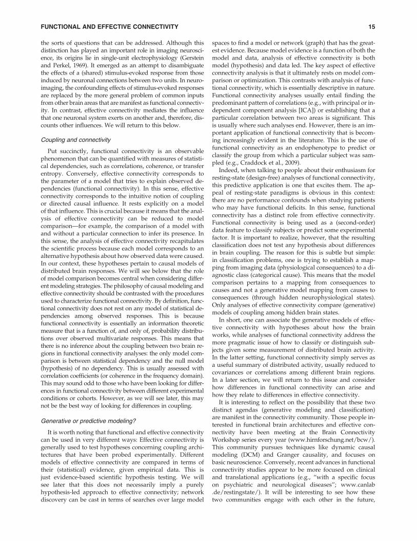
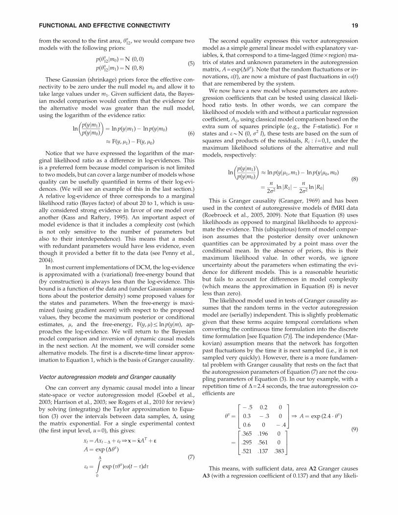
Here, we will establish the key dichotomies, or axes, thatframe the analysis of brain connectivity in both a practicaland a conceptual sense. The first distinction we consider is be-tween functional segregation and integration. This distinctionhas a deep history, which has guided much of brain mappingover the past two decades. A great deal of brain mapping isconcerned with functional segregation and the localizationof function. However, last year the annual increase in publi-cations on connectivity surpassed the yearly increase in pub-lications on activations per se (see Fig. 1). This may reflect ashift in emphasis from functional segregation to integration:the analysis of distributed and connected processing appealsto the notion of functional integration among segregatedbrain areas and rests on the key distinction between func-tional and effective connectivity. We will see that this distinc-tion not only has procedural and statistical implications fordata analysis but also is partly responsible for a segregationof the imaging neuroscience community interested in these is-sues. The material in this section borrows from its original for-mulation in Friston et al. (1993) and an early synthesis inFriston (1995).

Functional segregation and integration

From a historical perspective, the distinction between func-tional segregation and functional integration relates to thedialectic between localizationism and connectionism that

The Wellcome Trust Centre for Neuroimaging, University College London, London, United Kingdom.

BRAIN CONNECTIVITYVolume 1, Number 1, 2011ª Mary Ann Liebert, Inc.DOI: 10.1089/brain.2011.0008

13

dominated ideas about brain function in the 19th century.Since the formulation of phrenology by Gall, the identifica-tion of a particular brain region with a specific function hasbecome a central theme in neuroscience. Somewhat ironically,the notion that distinct brain functions could be localized wasstrengthened by early attempts to refute phrenology. In 1808,a scientific committee of the Athenee at Paris, chaired by Cuv-ier, declared that phrenology was unscientific and invalid(Staum, 1995). This conclusion may have been influencedby Napoleon Bonaparte (after an unflattering examinationof his skull by Gall). During the following decades, lesionand electrical stimulation paradigms were developed to testwhether functions could indeed be localized in animals. Theinitial findings of experiments by Flourens on pigeons wereincompatible with phrenologist predictions, but later experi-ments, including stimulation experiments in dogs and mon-keys by Fritsch, Hitzig, and Ferrier, supported the idea thatthere was a relation between distinct brain regions and spe-cific functions. Further, clinicians like Broca and Wernickeshowed that patients with focal brain lesions showed specificimpairments. However, it was realized early on that it wasdifficult to attribute a specific function to a cortical area,given the dependence of cerebral activity on the anatomicalconnections between distant brain regions. For example, ameeting that took place on August 4, 1881, addressed the dif-ficulties of attributing function to a cortical area given the de-pendence of cerebral activity on underlying connections(Phillips et al., 1984). This meeting was entitled Localizationof Function in the Cortex Cerebri. Goltz (1881), althoughaccepting the results of electrical stimulation in dog and mon-key cortex, considered the excitation method inconclusive, inthat the movements elicited might have originated in relatedpathways or current could have spread to distant centers. Inshort, the excitation method could not be used to infer func-tional localization because localizationism discounted inter-actions or functional integration among different brainareas. It was proposed that lesion studies could supplementexcitation experiments. Ironically, it was observations on pa-tients with brain lesions several years later (see Absher andBenson, 1993) that led to the concept of disconnection syn-

dromes and the refutation of localizationism as a completeor sufficient account of cortical organization. Functional local-ization implies that a function can be localized in a corticalarea, whereas segregation suggests that a cortical area is spe-cialized for some aspects of perceptual or motor processing,and that this specialization is anatomically segregated withinthe cortex. The cortical infrastructure supporting a singlefunction may then involve many specialized areas whoseunion is mediated by the functional integration amongthem. In this view, functional segregation is only meaningfulin the context of functional integration and vice versa.

Functional and effective connectivity

Imaging neuroscience has firmly established functionalsegregation as a principle of brain organization in humans.The integration of segregated areas has proven more difficultto assess. One approach to characterize integration is in termsof functional connectivity, which is usually inferred on thebasis of correlations among measurements of neuronal activ-ity. Functional connectivity is defined as statistical dependen-cies among remote neurophysiological events. However,correlations can arise in a variety of ways. For example, in mul-tiunit electrode recordings, correlations can result from stimu-lus-locked transients evoked by a common input or reflectstimulus-induced oscillations mediated by synaptic connec-tions (Gerstein and Perkel, 1969). Integration within a distrib-uted system is usually better understood in terms of effectiveconnectivity: effective connectivity refers explicitly to the influ-ence that one neural system exerts over another, either at a syn-aptic or population level. Aertsen and Preißl (1991) proposedthat ‘‘effective connectivity should be understood as the exper-iment and time-dependent, simplest possible circuit diagramthat would replicate the observed timing relationships be-tween the recorded neurons.’’ This speaks to two importantpoints: effective connectivity is dynamic (activity-dependent),and depends on a model of interactions or coupling.

The operational distinction between functional and effec-tive connectivity is important because it determines the na-ture of the inferences made about functional integration and

FIG. 1. Publication rates pertaining to functional segregation and integration. Publications per year searching for ‘‘Activa-tion’’ or ‘‘Connectivity’’ and functional imaging. This reflects the proportion of studies looking at functional segregation (ac-tivation) and those looking at integration (connectivity). Source: PubMed.gov. U.S. National Library of Medicine. The imageon the left is from the front cover of The American Phrenological Journal: Vol. 10, No. 3 (March) 1846.

14 FRISTON

the sorts of questions that can be addressed. Although thisdistinction has played an important role in imaging neurosci-ence, its origins lie in single-unit electrophysiology (Gersteinand Perkel, 1969). It emerged as an attempt to disambiguatethe effects of a (shared) stimulus-evoked response from thoseinduced by neuronal connections between two units. In neuro-imaging, the confounding effects of stimulus-evoked responsesare replaced by the more general problem of common inputsfrom other brain areas that are manifest as functional connectiv-ity. In contrast, effective connectivity mediates the influencethat one neuronal system exerts on another and, therefore, dis-counts other influences. We will return to this below.

Coupling and connectivity

Put succinctly, functional connectivity is an observablephenomenon that can be quantified with measures of statisti-cal dependencies, such as correlations, coherence, or transferentropy. Conversely, effective connectivity corresponds tothe parameter of a model that tries to explain observed de-pendencies (functional connectivity). In this sense, effectiveconnectivity corresponds to the intuitive notion of couplingor directed causal influence. It rests explicitly on a modelof that influence. This is crucial because it means that the anal-ysis of effective connectivity can be reduced to modelcomparison—for example, the comparison of a model withand without a particular connection to infer its presence. Inthis sense, the analysis of effective connectivity recapitulatesthe scientific process because each model corresponds to analternative hypothesis about how observed data were caused.In our context, these hypotheses pertain to causal models ofdistributed brain responses. We will see below that the roleof model comparison becomes central when considering differ-ent modeling strategies. The philosophy of causal modeling andeffective connectivity should be contrasted with the proceduresused to characterize functional connectivity. By definition, func-tional connectivity does not rest on any model of statistical de-pendencies among observed responses. This is becausefunctional connectivity is essentially an information theoreticmeasure that is a function of, and only of, probability distribu-tions over observed multivariate responses. This means thatthere is no inference about the coupling between two brain re-gions in functional connectivity analyses: the only model com-parison is between statistical dependency and the null model(hypothesis) of no dependency. This is usually assessed withcorrelation coefficients (or coherence in the frequency domain).This may sound odd to those who have been looking for differ-ences in functional connectivity between different experimentalconditions or cohorts. However, as we will see later, this maynot be the best way of looking for differences in coupling.

Generative or predictive modeling?

It is worth noting that functional and effective connectivitycan be used in very different ways: Effective connectivity isgenerally used to test hypotheses concerning coupling archi-tectures that have been probed experimentally. Differentmodels of effective connectivity are compared in terms oftheir (statistical) evidence, given empirical data. This isjust evidence-based scientific hypothesis testing. We willsee later that this does not necessarily imply a purelyhypothesis-led approach to effective connectivity; networkdiscovery can be cast in terms of searches over large model

spaces to find a model or network (graph) that has the great-est evidence. Because model evidence is a function of both themodel and data, analysis of effective connectivity is bothmodel (hypothesis) and data led. The key aspect of effectiveconnectivity analysis is that it ultimately rests on model com-parison or optimization. This contrasts with analysis of func-tional connectivity, which is essentially descriptive in nature.Functional connectivity analyses usually entail finding thepredominant pattern of correlations (e.g., with principal or in-dependent component analysis [ICA]) or establishing that aparticular correlation between two areas is significant. Thisis usually where such analyses end. However, there is an im-portant application of functional connectivity that is becom-ing increasingly evident in the literature. This is the use offunctional connectivity as an endophenotype to predict orclassify the group from which a particular subject was sam-pled (e.g., Craddock et al., 2009).

Indeed, when talking to people about their enthusiasm forresting-state (design-free) analyses of functional connectivity,this predictive application is one that excites them. The ap-peal of resting-state paradigms is obvious in this context:there are no performance confounds when studying patientswho may have functional deficits. In this sense, functionalconnectivity has a distinct role from effective connectivity.Functional connectivity is being used as a (second-order)data feature to classify subjects or predict some experimentalfactor. It is important to realize, however, that the resultingclassification does not test any hypothesis about differencesin brain coupling. The reason for this is subtle but simple:in classification problems, one is trying to establish a map-ping from imaging data (physiological consequences) to a di-agnostic class (categorical cause). This means that the modelcomparison pertains to a mapping from consequences tocauses and not a generative model mapping from causes toconsequences (through hidden neurophysiological states).Only analyses of effective connectivity compare (generative)models of coupling among hidden brain states.

In short, one can associate the generative models of effec-tive connectivity with hypotheses about how the brainworks, while analyses of functional connectivity address themore pragmatic issue of how to classify or distinguish sub-jects given some measurement of distributed brain activity.In the latter setting, functional connectivity simply serves asa useful summary of distributed activity, usually reduced tocovariances or correlations among different brain regions.In a later section, we will return to this issue and considerhow differences in functional connectivity can arise andhow they relate to differences in effective connectivity.

It is interesting to reflect on the possibility that these twodistinct agendas (generative modeling and classification)are manifest in the connectivity community. Those people in-terested in functional brain architectures and effective con-nectivity have been meeting at the Brain ConnectivityWorkshop series every year (www.hirnforschung.net/bcw/).This community pursues techniques like dynamic causalmodeling (DCM) and Granger causality, and focuses onbasic neuroscience. Conversely, recent advances in functionalconnectivity studies appear to be more focused on clinicaland translational applications (e.g., ‘‘with a specific focuson psychiatric and neurological diseases’’; www.canlab.de/restingstate/). It will be interesting to see how thesetwo communities engage with each other in the future,

FUNCTIONAL AND EFFECTIVE CONNECTIVITY 15

especially as the agendas of both become broader and lessdistinct. This may be particularly important for a mechanis-tic understanding of disconnection syndromes and otherdisturbances of distributed processing. Further, there is agrowing appreciation that classification models (mappingfrom consequences to causes) may be usefully constrainedby generative models (mapping from causes to conse-quences). For example, generative models can be used toconstruct an interpretable and sparse feature-space for sub-sequent classification. This ‘‘generative embedding’’ was in-troduced by Brodersen and associates (2011a), who useddynamic causal models of local field potential recordingsfor single-trial decoding of cognitive states. This approachmay be particularly attractive for clinical applications,such as classification of disease mechanisms in individualpatients (Brodersen et al., 2011b). Before turning to the tech-nical and pragmatic implications of functional and effectiveconnectivity, we consider structural or anatomical connec-tivity that has been referred to, appealingly, as the connec-tome (Sporns et al., 2005).

Connectivity and the connectome

In the many reviews and summaries of the definitions usedin brain connectivity research (e.g., Guye et al., 2008; Sporns,2007), researchers have often supplemented functional andeffective connectivity with structural connectivity. In recentyears, the fundamental importance of large-scale anatomicalinfrastructures that support effective connections for cou-pling has reemerged in the context of the connectome and at-tendant graph theoretical treatments (Bassett and Bullmore,2009; Bullmore and Sporns, 2009; Sporns et al., 2005). Thismay, in part, reflect the availability of probabilistic tractogra-phy measures of extrinsic (between area) connections fromdiffusion tensor imaging (Behrens and Johansen-Berg,2005). The status of structural connectivity and its relation-ship to functional effective connectivity is interesting. I seestructural connectivity as furnishing constraints or prior be-liefs about effective connectivity. In other words, effectiveconnectivity depends on structural connectivity, but struc-tural connectivity per se is neither a sufficient nor a completedescription of connectivity.

I have heard it said that if we had complete access to the con-nectome, we would understand how the brain works. I suspectthat most people would not concur with this; it presupposesthat brain connectivity possesses some invariant propertythat can be captured anatomically. However, this is not thecase. Synaptic connections in the brain are in a state of constantflux showing exquisite context-sensitivity and time- or activity-dependent effects (e.g., Saneyoshi et al., 2010). These are man-ifest over a vast range of timescales, from synaptic depressionover a few milliseconds (Abbott et al., 1997) to the maintenanceof long-term potentiation over weeks. In particular, there aremany biophysical mechanisms that underlie fast, nonlinear‘‘gating’’ of synaptic inputs, such as voltage-dependent ionchannels and phosphorylation of glutamatergic receptors bydopamine (Wolf et al., 2003). Even structural connectivitychanges over time, at microscopic (e.g., the cycling of postsyn-aptic receptors between the cytosol and postsynaptic mem-brane) and macroscopic (e.g., neurodevelopmental) scales.Indeed, most analyses of effective connectivity focus specifi-cally on context- or condition-specific changes in connectivity

that are mediated by changes in cognitive set or unfold overtime due to synaptic plasticity. These sorts of effects have mo-tivated the development of nonlinear models of effective con-nectivity that consider explicitly interactions among synapticinputs (e.g., Friston et al., 1995; Stephan et al., 2008). In short,connectivity is as transient, adaptive, and context-sensitive asbrain activity per se. Therefore, it is unlikely that characteriza-tions of connectivity that ignore this will furnish deep insightsinto distributed processing. So what is the role of structuralconnectivity?

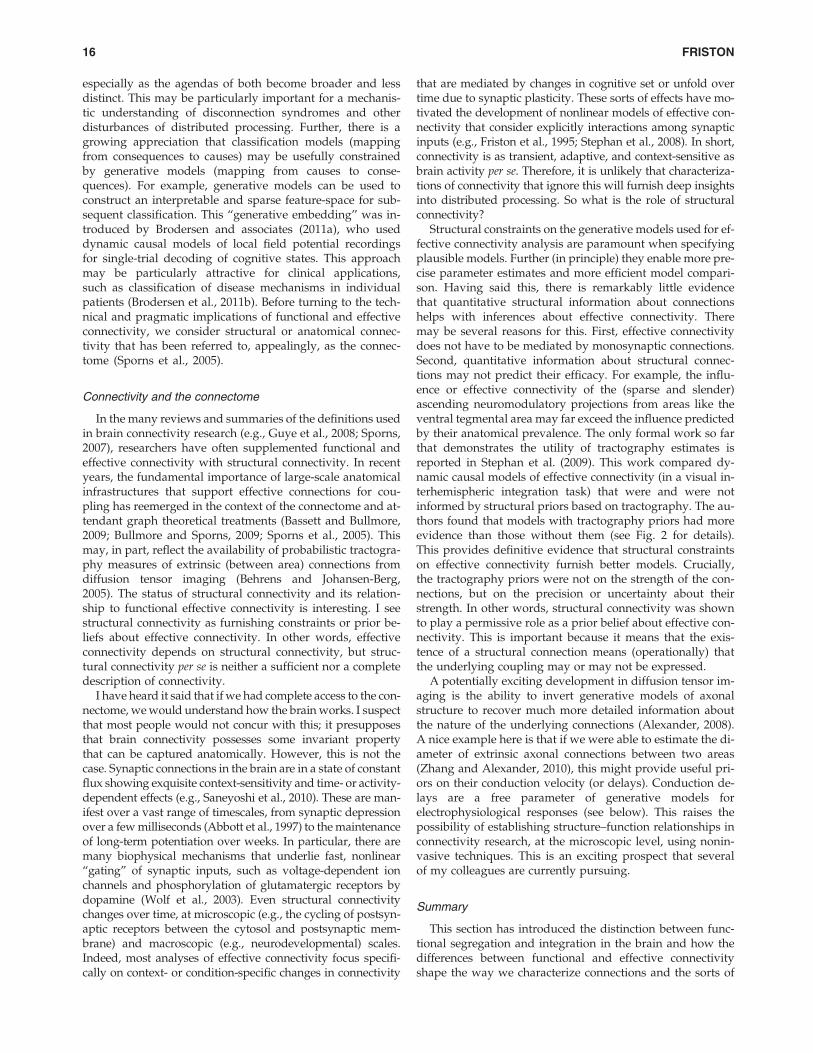
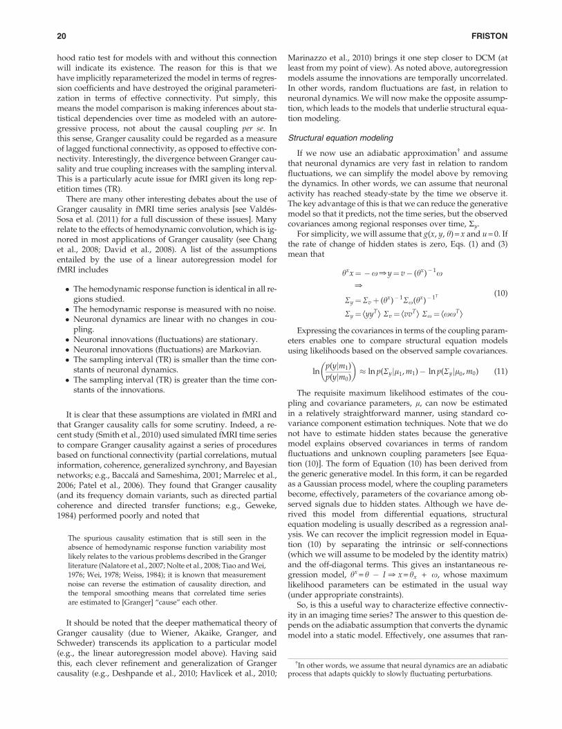
Structural constraints on the generative models used for ef-fective connectivity analysis are paramount when specifyingplausible models. Further (in principle) they enable more pre-cise parameter estimates and more efficient model compari-son. Having said this, there is remarkably little evidencethat quantitative structural information about connectionshelps with inferences about effective connectivity. Theremay be several reasons for this. First, effective connectivitydoes not have to be mediated by monosynaptic connections.Second, quantitative information about structural connec-tions may not predict their efficacy. For example, the influ-ence or effective connectivity of the (sparse and slender)ascending neuromodulatory projections from areas like theventral tegmental area may far exceed the influence predictedby their anatomical prevalence. The only formal work so farthat demonstrates the utility of tractography estimates isreported in Stephan et al. (2009). This work compared dy-namic causal models of effective connectivity (in a visual in-terhemispheric integration task) that were and were notinformed by structural priors based on tractography. The au-thors found that models with tractography priors had moreevidence than those without them (see Fig. 2 for details).This provides definitive evidence that structural constraintson effective connectivity furnish better models. Crucially,the tractography priors were not on the strength of the con-nections, but on the precision or uncertainty about theirstrength. In other words, structural connectivity was shownto play a permissive role as a prior belief about effective con-nectivity. This is important because it means that the exis-tence of a structural connection means (operationally) thatthe underlying coupling may or may not be expressed.

A potentially exciting development in diffusion tensor im-aging is the ability to invert generative models of axonalstructure to recover much more detailed information aboutthe nature of the underlying connections (Alexander, 2008).A nice example here is that if we were able to estimate the di-ameter of extrinsic axonal connections between two areas(Zhang and Alexander, 2010), this might provide useful pri-ors on their conduction velocity (or delays). Conduction de-lays are a free parameter of generative models forelectrophysiological responses (see below). This raises thepossibility of establishing structure–function relationships inconnectivity research, at the microscopic level, using nonin-vasive techniques. This is an exciting prospect that severalof my colleagues are currently pursuing.

Summary

This section has introduced the distinction between func-tional segregation and integration in the brain and how thedifferences between functional and effective connectivityshape the way we characterize connections and the sorts of

16 FRISTON

questions that are addressed. We have touched upon the roleof structural connectivity in providing constraints on the ex-pression of effective connectivity or coupling among neuro-nal systems. In the next section, we look at the relationshipbetween functional and effective connectivity and how theformer depends upon the latter.

Analyzing Connectivity

This section looks more formally at functional and effectiveconnectivity, starting with a generic (state-space) model of theneuronal systems that we are trying to characterize. This nec-essarily entails a generative model and, implicitly, frames theproblem in terms of effective connectivity. We will look atways of identifying the parameters of these models and com-paring different models statistically. In particular, we will con-sider successive approximations that lead to simpler modelsand procedures commonly employed to analyze connectivity.In doing this, we will hopefully see the relationships among thedifferent analyses and the assumptions on which they rest. Tomake this section as clear as possible, it will use a toy exampleto quantify the implications of various assumptions. This ex-ample uses a plausible connectivity architecture and showshow changes in coupling, under different experimental condi-tions or cohorts, would be manifest as changes in effective orfunctional connectivity. This section concludes with a heuristic

discussion of how to compare connectivity between conditionsor groups. The material here is a bit technical but uses a tutorialstyle that tries to suppress unnecessary mathematical details(with a slight loss of rigor and generality).

A generative model of coupled neuronal systems

We start with a generic description of distributed neuronaland other physiological dynamics, in terms of differentialequations. These equations describe the motion or flow,f(x, u, h), of hidden neuronal and physiological states, x(t),such as synaptic activity and blood volume. These statesare hidden because they are not observed directly. Thismeans we also have to specify mapping, g(x, u, h), fromhidden states to observed responses, y(t):

_x¼ f (x, u, h)þx

y¼ g(x, u, h)þ v(1)

Here, u(t) corresponds to exogenous inputs that might en-code changes in experimental conditions or the context underwhich the responses were observed. Random fluctuationsx(t) and v(t) on the motion of hidden states and observa-tions render Equation (1) a random or stochastic differentialequation. One might wonder why we need both exogenous(deterministic) and endogenous (random) inputs; whereasthe exogenous inputs are generally known and under experi-

FIG. 2. Structural con-straints on functional connec-tions. This schematicillustrates the procedurereported in Stephan et al.(2009), providing evidencethat anatomical tractographymeasures provide informa-tive constraints on modelsand effective connectivity.Consider the problem of esti-mating the effective connec-tivity among some regions,given quantitative (if proba-bilistic) estimates of their an-atomical connection strengths(demoted by uij). This is il-lustrated in the lower leftpanel using bilateral areas inthe lingual and fusiform gyri.The first step would be tospecify some mapping be-tween the anatomical infor-mation and prior beliefsabout the effective connec-tions. This mapping is illus-trated in the upper left panel,by expressing the prior vari-ance on effective connectivity(model parameters h) as asigmoid function of anatomi-cal connectivity, with un-

known hyperparameters a b � m, where m denotes a model. We can now optimize the model in terms of its hyperparametersand select the model with the highest evidence p(yjm), as illustrated by model scoring on the upper right. When this was doneusing empirical data, tractography priors were found to have a sensible and quantitatively important role. The inset on thelower right shows the optimum relationship between tractography estimates and prior variance constraints on effectiveconnectivity. The four asterisks correspond to the four tractography measures shown on the lower left [see Stephan et al. (2009)for further detail].


mental control, endogenous inputs represent unknown influ-ences (e.g., from areas not in the model or spontaneous fluctu-ations). These can only be modeled probabilistically (usuallyunder Gaussian, and possibly Markovian, assumptions).

Clearly, the equations of motion (first equality) and observerfunction (second equality) are, in reality, immensely compli-cated equations of very large numbers of hidden states. Inpractice, there are various theorems such as the center mani-fold theorem* and slaving principle, which means one can re-duce the effective number of hidden states substantially butstill retain the underlying dynamical structure of the system(Ginzburg and Landau, 1950; Carr, 1981; Haken, 1983; Kopelland Ermentrout, 1986). The parameters of these equations, h,include effective connectivity and control how hidden statesin one part of the brain affect the motion of hidden states else-where. Equation (1) can be regarded as a generative model ofobserved data that is specified completely, given assumptionsabout the random fluctuations and prior beliefs about thestates and parameters. Inverting or fitting this generativemodel corresponds to estimating its unknown states and pa-rameters (effective connectivity), given some observed data.This is called dynamic causal modeling (DCM) and usuallyemploys Bayesian techniques.

However, the real power of DCM lies in the ability to com-pare different models of the same data. This comparison restson the model evidence, which is simply the probability of theobserved data, under the model in question (and known ex-ogenous inputs). The evidence is also called the marginal like-lihood because one marginalizes or removes dependencies onthe unknown quantities (states and parameters).

p(yjm, u)¼Z

p(y, x, hjm, u)dxdh (2)

Model comparison rests on the relative evidence for onemodel compared to another [see Penny et al. (2004) for adiscussion in the context of functional magnetic resonanceimaging (fMRI). Likelihood-ratio tests of this sort are com-monplace. Indeed, one can cast the t-statistic as a likelihoodratio. Model comparison based on the likelihood of differentmodels will be a central theme in this review and provides thequantitative basis for all evidence-based hypothesis testing.In this section, we will see that all analyses of effective con-nectivity can be reduced to model comparison. This meansthe crucial differences among these analyses rest with themodels on which they are based.

Clearly, to search over all possible models (to find the onewith the most evidence) is generally impossible. One, there-fore, appeals to simplified but plausible models. To illustratethis simplification and to create an illustrative toy example,we will use a local (bilinear) approximation to Equation (1)of the sort used in DCM of fMRI time series (Friston et al.,2003) and with a single exogenous input, u 2 f0, 1g:

_x¼ hxxþ uhxuxþ huuþx

hx¼ vf

vxhxu¼ v2f

vxvuhu¼ vf

vu

��x¼ 0, u¼ 0

(3)

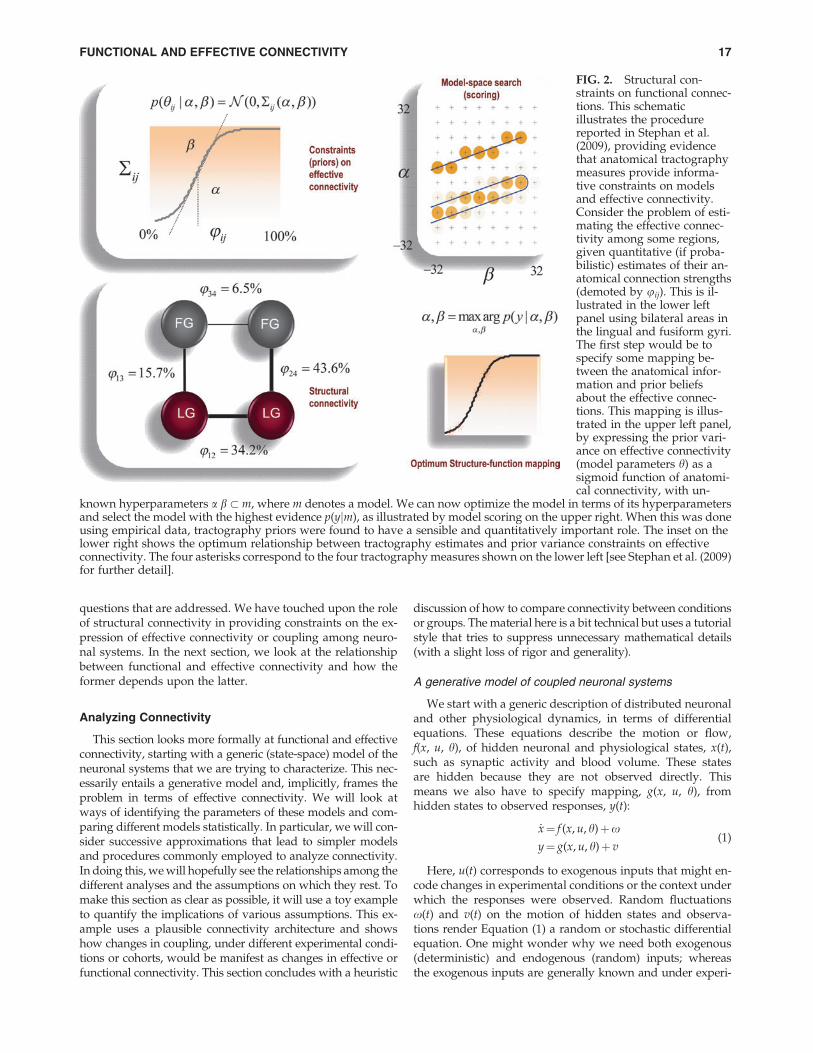
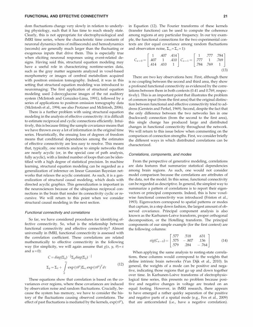
Here, superscripts indicate whether the parameters refer tothe strength of connections, hx, their context-dependent (bilin-ear) modulation, hxu, or the effects of perturbations or exoge-nous inputs, hu. To keep things very simple, we will furtherpretend that we have direct access to hidden neuronal statesand that they are measured directly (as in invasive electro-physiology). This means we can ignore hemodynamics andthe observer function (for now). Equation (3) parameterizesconnectivity in terms of partial derivatives of the state-equation. For example, the network in Figure 3 can be de-scribed with the following effective connectivity parameters:

hx¼� :5 0:2 0

0:3 �:3 0

0:6 0 �:4

264

375 hxu¼

0 0:2 0

0 0 0

0 0 0

264

375 hu¼

0

0

0

264375 (4)

Here, the input u 2 f0, 1g encodes a condition or cohort-spe-cific effect that selectively increases the (backward) couplingfrom the second to the first node or region (from now onwe will use effective connectivity and coupling synonymous-ly). These values have been chosen as fairly typical for fMRI.Note that the exogenous inputs do not exert a direct (activat-ing) effect on hidden states, but act to increase a particularconnection and endow it with context-sensitivity. Note fur-ther that we have assumed that hidden neuronal dynamicscan be captured with a single state for each area. We willnow consider the different ways in which one can try to esti-mate these parameters.

Dynamic causal modeling

As noted above, DCM would first select the best modelusing Bayesian model comparison. Usually, different modelsare specified in terms of priors on the coupling parameters.These are used to switch off parameters by assuming a priorithat they are zero (to create a new model). For example, if wewanted to test for the presence of a backward connection

FIG. 3. Toy connectivity architecture. This schematic showsthe connections among three brain areas or nodes that will beused to demonstrate the relationship between effective con-nectivity and functional connectivity in the main text. Tohighlight the role of changes in connectivity, the right graphshows the connection that changes (over experimental condi-tion or diagnostic cohort) as the thick black line. This is an ex-ample of a directed cyclic graph. It is cyclic by virtue of thereciprocal connections between A1 and A2.

*Strictly speaking, the center manifold theorem is used to reducethe degrees of freedom only in the neighborhood of a bifurcation.

18 FRISTON

from the second to the first area, hx12, we would compare two

models with the following priors:

p(hx12jm0)¼N (0, 0)

p(hx12jm1)¼N (0, 8)

(5)

These Gaussian (shrinkage) priors force the effective con-nectivity to be zero under the null model m0 and allow it totake large values under m1. Given sufficient data, the Bayes-ian model comparison would confirm that the evidence forthe alternative model was greater than the null model,using the logarithm of the evidence ratio:

lnp(yjm1)

p(yjm0)

� �¼ ln p(yjm1)� ln p(yjm0)

� F(y, l1)� F(y, l0)

(6)

Notice that we have expressed the logarithm of the mar-ginal likelihood ratio as a difference in log-evidences. Thisis a preferred form because model comparison is not limitedto two models, but can cover a large number of models whosequality can be usefully quantified in terms of their log-evi-dences. (We will see an example of this in the last section.)A relative log-evidence of three corresponds to a marginallikelihood ratio (Bayes factor) of about 20 to 1, which is usu-ally considered strong evidence in favor of one model overanother (Kass and Raftery, 1995). An important aspect ofmodel evidence is that it includes a complexity cost (whichis not only sensitive to the number of parameters butalso to their interdependence). This means that a modelwith redundant parameters would have less evidence, eventhough it provided a better fit to the data (see Penny et al.,2004).

In most current implementations of DCM, the log-evidenceis approximated with a (variational) free-energy bound that(by construction) is always less than the log-evidence. Thisbound is a function of the data and (under Gaussian assump-tions about the posterior density) some proposed values forthe states and parameters. When the free-energy is maxi-mized (using gradient ascent) with respect to the proposedvalues, they become the maximum posterior or conditionalestimates, l, and the free-energy, F(y, l)p ln p(yjm), ap-proaches the log-evidence. We will return to the Bayesianmodel comparison and inversion of dynamic causal modelsin the next section. At the moment, we will consider somealternative models. The first is a discrete-time linear approx-imation to Equation 1, which is the basis of Granger causality.

Vector autoregression models and Granger causality

One can convert any dynamic causal model into a linearstate-space or vector autoregression model (Goebel et al.,2003; Harrison et al., 2003; see Rogers et al., 2010 for review)by solving (integrating) the Taylor approximation to Equa-tion (3) over the intervals between data samples, D, usingthe matrix exponential. For a single experimental context(the first input level, u = 0), this gives:

xt¼Axt�Dþ et0x¼ ~xAT þ e

A¼ exp (Dhx)

et¼ZD

0

exp (shx)x(t� s)ds

(7)

The second equality expresses this vector autoregressionmodel as a simple general linear model with explanatory var-iables, ~x, that correspond to a time-lagged (time · region) ma-trix of states and unknown parameters in the autoregressionmatrix, A = exp(Dhx). Note that the random fluctuations or in-novations, e(t), are now a mixture of past fluctuations in x(t)that are remembered by the system.

We now have a new model whose parameters are autore-gression coefficients that can be tested using classical likeli-hood ratio tests. In other words, we can compare thelikelihood of models with and without a particular regressioncoefficient, Aij, using classical model comparison based on theextra sum of squares principle (e.g., the F-statistic). For nstates and e*N (0, r2 I), these tests are based on the sum ofsquares and products of the residuals, Ri : i = 0,1, under themaximum likelihood solutions of the alternative and nullmodels, respectively:

lnp(yjm1)

p(yjm0)

� �� ln p(yjl1, m1)� ln p(yjl0, m0)

¼ n

2r2ln jR1j �

n

2r2ln jR0j

(8)

This is Granger causality (Granger, 1969) and has beenused in the context of autoregressive models of fMRI data(Roebroeck et al., 2005, 2009). Note that Equation (8) useslikelihoods as opposed to marginal likelihoods to approxi-mate the evidence. This (ubiquitous) form of model compar-ison assumes that the posterior density over unknownquantities can be approximated by a point mass over theconditional mean. In the absence of priors, this is theirmaximum likelihood value. In other words, we ignoreuncertainty about the parameters when estimating the evi-dence for different models. This is a reasonable heuristicbut fails to account for differences in model complexity(which means the approximation in Equation (8) is neverless than zero).

The likelihood model used in tests of Granger causality as-sumes that the random terms in the vector autoregressionmodel are (serially) independent. This is slightly problematicgiven that these terms acquire temporal correlations whenconverting the continuous time formulation into the discretetime formulation [see Equation (7)]. The independence (Mar-kovian) assumption means that the network has forgottenpast fluctuations by the time it is next sampled (i.e., it is notsampled very quickly). However, there is a more fundamen-tal problem with Granger causality that rests on the fact thatthe autoregression parameters of Equation (7) are not the cou-pling parameters of Equation (3). In our toy example, with arepetition time of D = 2.4 seconds, the true autoregression co-efficients are

hx¼� :5 0:2 0

0:3 � :3 0

0:6 0 � :4

264

3750 A¼ exp (2:4 � hx)

¼:365 :196 0

:295 :561 0

:521 :137 :383

264

375

(9)

This means, with sufficient data, area A2 Granger causesA3 (with a regression coefficient of 0.137) and that any likeli-


hood ratio test for models with and without this connectionwill indicate its existence. The reason for this is that wehave implicitly reparameterized the model in terms of regres-sion coefficients and have destroyed the original parameteri-zation in terms of effective connectivity. Put simply, thismeans the model comparison is making inferences about sta-tistical dependencies over time as modeled with an autore-gressive process, not about the causal coupling per se. Inthis sense, Granger causality could be regarded as a measureof lagged functional connectivity, as opposed to effective con-nectivity. Interestingly, the divergence between Granger cau-sality and true coupling increases with the sampling interval.This is a particularly acute issue for fMRI given its long rep-etition times (TR).

There are many other interesting debates about the use ofGranger causality in fMRI time series analysis [see Valdes-Sosa et al. (2011) for a full discussion of these issues]. Manyrelate to the effects of hemodynamic convolution, which is ig-nored in most applications of Granger causality (see Changet al., 2008; David et al., 2008). A list of the assumptionsentailed by the use of a linear autoregression model forfMRI includes

� The hemodynamic response function is identical in all re-gions studied.� The hemodynamic response is measured with no noise.� Neuronal dynamics are linear with no changes in cou-

pling.� Neuronal innovations (fluctuations) are stationary.� Neuronal innovations (fluctuations) are Markovian.� The sampling interval (TR) is smaller than the time con-

stants of neuronal dynamics.� The sampling interval (TR) is greater than the time con-

stants of the innovations.

It is clear that these assumptions are violated in fMRI andthat Granger causality calls for some scrutiny. Indeed, a re-cent study (Smith et al., 2010) used simulated fMRI time seriesto compare Granger causality against a series of proceduresbased on functional connectivity (partial correlations, mutualinformation, coherence, generalized synchrony, and Bayesiannetworks; e.g., Baccala and Sameshima, 2001; Marrelec et al.,2006; Patel et al., 2006). They found that Granger causality(and its frequency domain variants, such as directed partialcoherence and directed transfer functions; e.g., Geweke,1984) performed poorly and noted that

The spurious causality estimation that is still seen in theabsence of hemodynamic response function variability mostlikely relates to the various problems described in the Grangerliterature (Nalatore et al., 2007; Nolte et al., 2008; Tiao and Wei,1976; Wei, 1978; Weiss, 1984); it is known that measurementnoise can reverse the estimation of causality direction, andthe temporal smoothing means that correlated time seriesare estimated to [Granger] ‘‘cause’’ each other.

It should be noted that the deeper mathematical theory ofGranger causality (due to Wiener, Akaike, Granger, andSchweder) transcends its application to a particular model(e.g., the linear autoregression model above). Having saidthis, each clever refinement and generalization of Grangercausality (e.g., Deshpande et al., 2010; Havlicek et al., 2010;

Marinazzo et al., 2010) brings it one step closer to DCM (atleast from my point of view). As noted above, autoregressionmodels assume the innovations are temporally uncorrelated.In other words, random fluctuations are fast, in relation toneuronal dynamics. We will now make the opposite assump-tion, which leads to the models that underlie structural equa-tion modeling.

Structural equation modeling

If we now use an adiabatic approximation{ and assumethat neuronal dynamics are very fast in relation to randomfluctuations, we can simplify the model above by removingthe dynamics. In other words, we can assume that neuronalactivity has reached steady-state by the time we observe it.The key advantage of this is that we can reduce the generativemodel so that it predicts, not the time series, but the observedcovariances among regional responses over time, Sy.

For simplicity, we will assume that g(x, y, h) = x and u = 0. Ifthe rate of change of hidden states is zero, Eqs. (1) and (3)mean that

hxx¼ �x0y¼ v� (hx)� 1x

0

Sy¼Svþ (hx)� 1Sx(hx)� 1T

Sy¼ ÆyyTæ Sv¼ ÆvvTæ Sx¼ ÆxxTæ

(10)

Expressing the covariances in terms of the coupling param-eters enables one to compare structural equation modelsusing likelihoods based on the observed sample covariances.

lnp(yjm1)

p(yjm0)

� �� ln p(Syjl1, m1)� ln p(Syjl0, m0) (11)

The requisite maximum likelihood estimates of the cou-pling and covariance parameters, l, can now be estimatedin a relatively straightforward manner, using standard co-variance component estimation techniques. Note that we donot have to estimate hidden states because the generativemodel explains observed covariances in terms of randomfluctuations and unknown coupling parameters [see Equa-tion (10)]. The form of Equation (10) has been derived fromthe generic generative model. In this form, it can be regardedas a Gaussian process model, where the coupling parametersbecome, effectively, parameters of the covariance among ob-served signals due to hidden states. Although we have de-rived this model from differential equations, structuralequation modeling is usually described as a regression anal-ysis. We can recover the implicit regression model in Equa-tion (10) by separating the intrinsic or self-connections(which we will assume to be modeled by the identity matrix)and the off-diagonal terms. This gives an instantaneous re-gression model, hx = h � I 0 x = hx + x, whose maximumlikelihood parameters can be estimated in the usual way(under appropriate constraints).

So, is this a useful way to characterize effective connectiv-ity in an imaging time series? The answer to this question de-pends on the adiabatic assumption that converts the dynamicmodel into a static model. Effectively, one assumes that ran-

{In other words, we assume that neural dynamics are an adiabaticprocess that adapts quickly to slowly fluctuating perturbations.

20 FRISTON

dom fluctuations change very slowly in relation to underly-ing physiology, such that it has time to reach steady state.Clearly, this is not appropriate for electrophysiological andfMRI time series, where the characteristic time constants ofneuronal dynamics (tens of milliseconds) and hemodynamics(seconds) are generally much larger than the fluctuating orexogenous inputs that drive them. This is especially truewhen eliciting neuronal responses using event-related de-signs. Having said this, structural equation modeling mayhave a useful role in characterizing nontime-series data,such as the gray matter segments analyzed in voxel-basedmorphometry or images of cerebral metabolism acquiredwith positron emission tomography. Indeed, it was in thissetting that structural equation modeling was introduced toneuroimaging: The first application of structural equationmodeling used 2-deoxyglucose images of the rat auditorysystem (McIntosh and Gonzalez-Lima, 1991), followed by aseries of applications to positron emission tomography data(McIntosh et al., 1994; see also Protzner and McIntosh, 2006).

There is a further problem with using structural equationmodeling in the analysis of effective connectivity: it is difficultto estimate reciprocal and cyclic connections efficiently. Intui-tively, this is because fitting the sample covariance means thatwe have thrown away a lot of information in the original timeseries. Heuristically, the ensuing loss of degrees of freedommeans that conditional dependencies among the estimatesof effective connectivity are less easy to resolve. This meansthat, typically, one restricts analyse to simple networks thatare nearly acyclic (or, in the special case of path analysis,fully acyclic), with a limited number of loops that can be iden-tified with a high degree of statistical precision. In machinelearning, structural equation modeling can be regarded as ageneralization of inference on linear Gaussian Bayesian net-works that relaxes the acyclic constraint. As such, it is a gen-eralization of structural causal modeling, which deals withdirected acyclic graphics. This generalization is important inthe neurosciences because of the ubiquitous reciprocal con-nections in the brain that render its connectivity cyclic or re-cursive. We will return to this point when we considerstructural causal modeling in the next section.

Functional connectivity and correlations

So far, we have considered procedures for identifying ef-fective connectivity. So, what is the relationship betweenfunctional connectivity and effective connectivity? Almostuniversally in fMRI, functional connectivity is assessed withthe correlation coefficient. These correlations are relatedmathematically to effective connectivity in the followingway (for simplicity, we will again assume that g(x, y, h) = xand u = 0):

C¼ diag(Sy)�12Sydiag(Sy)�

12

Sy¼SvþZ1

0

exp (shx)Sx exp (shx)Tds(12)

These equations show that correlation is based on the co-variances over regions, where these covariances are inducedby observation noise and random fluctuations. Crucially, be-cause the system has memory, we have to consider the his-tory of the fluctuations causing observed correlations. Theeffect of past fluctuations is mediated by the kernels, exp(shx),

in Equation (12). The Fourier transforms of these kernels(transfer functions) can be used to compute the coherenceamong regions at any particular frequency. In our toy exam-ple, the functional connections for the two experimental con-texts are (for equal covariance among random fluctuationsand observation noise, Sx =Sv = 1):

Cu¼ 0¼1 :407 :414:407 1 :410:414 :410 1

24

35Cu¼ 1¼

1 :777 :784:777 1 :769:784 :769 1

24

35

(13)

There are two key observations here. First, although thereis no coupling between the second and third area, they showa profound functional connectivity as evidenced by the corre-lations between them in both contexts (0.41 and 0.769, respec-tively). This is an important point that illustrates the problemof common input (from the first area) that the original distinc-tion between functional and effective connectivity tried to ad-dress (Gerstein and Perkel, 1969). Second, despite the fact thatthe only difference between the two networks lies in one(backward) connection (from the second to the first area),this single change has produced large and distributedchanges in functional connectivity throughout the network.We will return to this issue below when commenting on thecomparison of connection strengths. First, we consider brieflythe different ways in which distributed correlations can becharacterized.

Correlations, components, and modes

From the perspective of generative modeling, correlationsare data features that summarize statistical dependenciesamong brain regions. As such, one would not considermodel comparison because the correlations are attributes ofthe data, not the model. In this sense, functional connectivitycan be regarded as descriptive. In general, the simplest way tosummarize a pattern of correlations is to report their eigen-vectors or principal components. Indeed, this is how voxel-wise functional connectivity was introduced (Friston et al.,1993). Eigenvectors correspond to spatial patterns or modesthat capture, in a step down fashion, the largest amount of ob-served covariance. Principal component analysis is alsoknown as the Karhunen-Loeve transform, proper orthogonaldecomposition, or the Hotelling transform. The principalcomponents of our simple example (for the first context) arethe following columns:

eig(Cu¼ 0)¼:577 :518 :631:575 � :807 :136:579 :284 � :764

24

35 (14)

When applying the same analysis to resting-state correla-tions, these columns would correspond to the weights thatdefine intrinsic brain networks (Van Dijk et al., 2010). Ingeneral, the weights of a mode can be positive and nega-tive, indicating those regions that go up and down togetherover time. In Karhunen-Loeve transforms of electrophysio-logical time series, this presents no problem because posi-tive and negative changes in voltage are treated on anequal footing. However, in fMRI research, there appearsto have emerged a rather quirky separation of the positiveand negative parts of a spatial mode (e.g., Fox et al., 2009)that are anticorrelated (i.e., have a negative correlation).


This may reflect the fact that the physiological interpreta-tion of activation and deactivation is not completely sym-metrical in fMRI. Another explanation may be related tothe fact that spatial modes are often identified using spatialindependent component analysis (ICA).

Independent component analysis. ICA has very similarobjectives to principal component analysis (PCA), but as-sumes the modes are driven by non-Gaussian random fluctu-ations (Calhoun and Adali, 2006; Kiviniemi et al., 2003;McKeown et al., 1998). If we reprieve the assumptions ofstructural equation modeling [Equation (10)], we can regardprincipal component analysis as based up the following gen-erative model:

x¼ �Wx

W¼ (hx)� 1

x ~ N(0,Sx)

(15)

By simply replacing Gaussian assumptions about randomfluctuations with non-Gaussian (supra-Gaussian) assump-tions, we can obtain the generative model on which ICA isbased. The aim of ICA is to identify the maximum likelihoodestimates of the mixing matrix, W = (hx)�1, given observed co-variances. These correspond to the modes above. However,when performing ICA over voxels in fMRI, there is one finaltwist. For computational reasons, it is easier to analyze samplecorrelations over voxels than to analyze the enormous (voxel ·voxel) matrix of correlations over time. Analyzing the smaller(time · time) matrix is known as spatial ICA (McKeown et al.,1998). [See Friston (1998) for an early discussion of the relativemerits of spatial and temporal ICA.] In the present context, thismeans that the modes are independent (and orthogonal) overspace and that the temporal expression of these independentcomponents may be correlated. Put plainly, this means that in-dependent components obtained by spatial ICA may or maynot be functionally connected in time. I make this point be-cause those from outside the fMRI community may be con-fused by the assertion that two spatial modes (intrinsic brainnetworks) are anticorrelated. This is because they might as-sume temporal ICA (or PCA) was used to identify themodes, which are (by definition) uncorrelated.

Changes in connectivity

So far, we have focused on comparing different models ornetwork architectures that best explain observed data. Wenow look more closely at inferring quantitative changes in cou-pling due to experimental manipulations. As noted above, thereis a profound difference between comparing effective connec-tion strengths and functional connectivity. In effective connec-tivity modeling, one usually makes inferences about couplingchanges by comparing models with and without an effect of ex-perimental context or cohort. These effects correspond to the bi-linear parameters hxu in Equation (3). If model comparisonsupported the evidence for the model with a context or cohorteffect, one would then conclude the associated connection (orconnections) had changed. However, when comparing func-tional connectivity, one cannot make any comment aboutchanges in coupling. Basically, showing that there is a differ-ence in the correlation between two areas does not mean thatthe coupling between these areas has changed; it only means

that there has been some change in the distributed activity ob-served in one context and another and that this change is man-ifest in the correlation [see Equation (13)]. Clearly, this is not aproblem if one is only interested in using correlations to predictthe cohort or condition from which data were sampled. How-ever, it is important not to interpret a difference in correlationas a change in coupling. The correlation coefficient reportsthe evidence for a statistical dependency between two areas,but changes in this dependency can arise without changes incoupling. This is particularly important for Granger causality,where it might be tempting to compare Granger causality, ei-ther between two experimental situations or between directedconnections between two nodes. In short, a difference in evi-dence (correlation, coherence, or Granger causality) shouldnot be taken as evidence for a difference in coupling. One canillustrate this important point with three examples of how achange in correlation could be observed in the absence of achange in effective connectivity.

Changes in another connection. Because functional con-nectivity can be expressed at a distance from changes in effec-tive connectivity, any observed change in the correlationbetween two areas can be easily caused by a coupling changeelsewhere. Using our example above, we can see immediatelythat the correlation between A1 and A2 changes when we in-crease the backward connection strength from A2 to A1.Quantitatively, this is evident from Equation (13), where:

DC¼Cu¼ 1�Cu¼ 0¼0 :369 :370:369 0 :359:370 :359 0

24

35 (16)

This is perfectly sensible and reflects the fact that statisticaldependencies among the nodes of a network are exquisitelysensitive to changes in coupling anywhere. So, does thismean a change in a correlation can be used to infer a changein coupling somewhere in the system? No, because the corre-lation can change without any change in coupling.

Changes in the level of observation noise. An importantfallacy of comparing correlation coefficients rests on the factthat correlations depend on the level of observation noise.This means that one can see a change in correlation by simplychanging the signal-to-noise ratio of the data. This can be par-ticularly important when comparing correlations betweendifferent groups of subjects. For example, obsessive compul-sive patients may have a heart rate variability that differsfrom normal subjects. This may change the noise in observedhemodynamic responses, even in the absence of neuronal dif-ferences or changes in effective connectivity. We can simulatethis effect, using Equation (12) above, where, using noise lev-els of Sv = 1 and Sv = 1.252, we obtain the following differencein correlations:

DC¼0 � :061 � :060

� :061 0 � :048� :060 � :048 0

24

35 (17)

These changes are just due to increasing the standard devi-ation of observation noise by 25%. This reduces the correla-tion because it changes with the noise level [see Equation(12)]. The ensuing difficulties associated with comparing cor-relations are well known in statistics and are related to the

22 FRISTON

problem of dilution or attenuation in regression problems(e.g., Spearman, 1904). If we ensured that the observationnoise was the same over different levels of an experimentalfactor, could we then infer some change in the underlyingconnectivity? Again, the answer is no because the correlationalso depends on the variance of hidden neuronal states, Sx,that can only be estimated under a generative model.

Changes in neuronal fluctuations. One can produce thesame sort of difference in correlations by changing the ampli-tude of neuronal fluctuations (designed or endogenous) with-out changing the coupling. As a quantitative example, fromEquation (12) we obtain the following difference in correla-tions when changing Sx = 1 to Sx = 1.252:

DC¼0 :053 :052:053 0 :038:052 :038 0

24

35 (18)

The possible explanations for differences in neuronalactivity between different cohorts of subjects, or indeeddifferent conditions, are obviously innumerable. Yet, anyof these differences can produce a change in functionalconnectivity.

These examples highlight the difficulties of interpretingdifferences in functional connectivity in relation to changesin the underlying coupling. Importantly, these argumentspertain to any measures reporting the evidence for statisticaldependencies, including coherence, mutual information,transfer entropy, and Granger causality. The fallacy of com-paring statistics in this way can be seen intuitively in termsof model comparison. Usually, one compares the evidencefor different models of the same data. When testing for achange in coupling, this entails comparing models that doand do not include a change in connectivity. This is not thesame as comparing the evidence for the same model of differ-ent data. A change in evidence here simply means the datahave changed. In short, a change in model evidence is not ev-idence for model of change.

As noted above, these interpretational issues may not berelevant when simply trying to establish group differencesor classify subjects. However, if one wants to make some spe-cific and mechanistic inference about the impact of an exper-imental manipulation on the coupling between particularbrain regions, he or she has to use effective connectivity. Hap-pily, there is a relatively straightforward way of doing this forfMRI that is less complicated than comparing correlations.

Psychophysiological interactions

Assume that we wanted to test the hypothesis that fronto-temporal coupling differed significantly between two groupsof subjects. Given the above arguments, we would comparemodels of effective connectivity that did and did not allowfor a change. One of the most basic model comparisons thatcan be implemented using standard linear convolution mod-els for fMRI is the test for a psychophysiological interaction.In this comparison, one tests for interactions between a phys-iological variable and a psychological variable or experimen-tal factor. This interaction is generally interpreted in terms ofan experimentally mediated change in (linear) effective con-nectivity between the area expressing a significant interactionand the seed or reference region from which the physiological

variable was harvested. At the between-subject or grouplevel, this reduces to a group difference between the regres-sion coefficient that is obtained from regressing the activityat any point in the brain on the activity of the seed region[see Kasahara et al. (2010) for a nice application]. It is this re-gression coefficient that can be associated with effective con-nectivity (i.e., change in activity per unit change in the seedregion). To test the null hypothesis that there is no group dif-ference in coupling, one simply performs a two sample t-teston the regression coefficients. The results of this whole-brainanalysis can be treated in the usual way to identify those re-gions whose effective connectivity with the reference regiondiffers significantly.

Note that this is very similar to a comparison of correla-tions with a seed region. The crucial difference is that thesummary statistic (summarizing the connectivity) reports ef-fective connectivity, not functional connectivity. This meansthat it is not confounded by differences in signal or noise,and (under the simple assumptions of a psychophysiologicalinteraction model) can be interpreted as a change in coupling.It should be said that there are many qualifications to theuse of these simple linear models of effective connectivity(because they belong to the class of structural equation or re-gression models; Friston et al., 1997). However, psychophys-iologic interactions are simple, intuitive, and (mildly)principled. Further, because the fluctuations in the physiolog-ical measure are typically slow in resting-state studies, theusual caveats of hemodynamic convolution can be ignored.

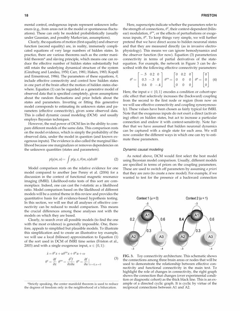
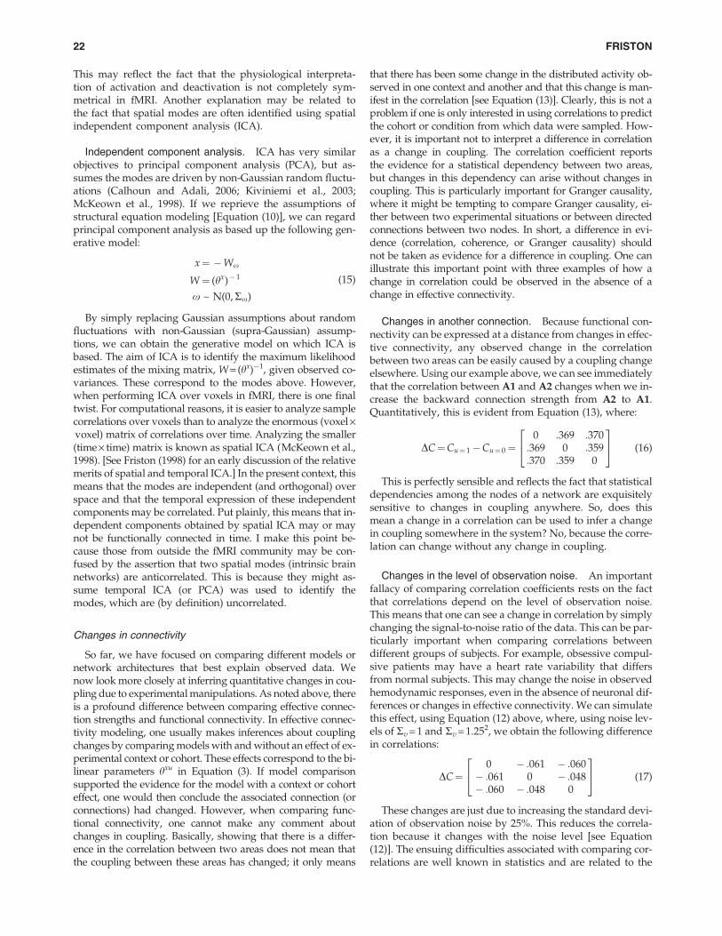
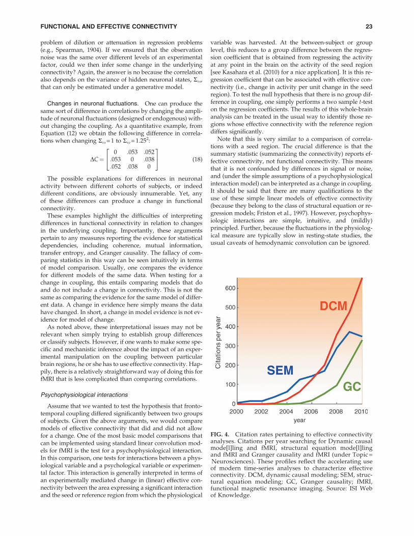
FIG. 4. Citation rates pertaining to effective connectivityanalyses. Citations per year searching for Dynamic causalmode[l]ling and fMRI, structural equation mode[l]lingand fMRI and Granger causality and fMRI (under Topic =Neurosciences). These profiles reflect the accelerating useof modern time-series analyses to characterize effectiveconnectivity. DCM, dynamic causal modeling; SEM, struc-tural equation modeling; GC, Granger causality; fMRI,functional magnetic resonance imaging. Source: ISI Webof Knowledge.


Summary

This section has tried to place different analyses of connec-tivity in relation to each other. The most prevalent approachesto effective connectivity analysis are DCM, structural equationmodeling, and Granger causality. All have enjoyed a rapid up-take over the past decade (see Fig. 4). This didactic (and polem-ic) treatment has highlighted some of the implicit andimplausible assumptions made when applying structuralequation modeling and Granger causality to fMRI time series.I personally find the recent upsurge of Granger causality infMRI worrisome, and it is difficult to know what to do whenasked to review these articles. In practice, I generally just askauthors to qualify their conclusions by listing the assumptionsthat underlie their analysis. On the one hand, it is importantthat people are not discouraged from advancing and applyingclassical time series analyses to fMRI. On the other hand, thepersistent use of models and procedures that are not fit for pur-pose may confound scientific progress in the long term. Per-haps, having written this, people will exclude me fromreviewing their articles on Granger causality and I will no lon-ger have to worry about these things. On a more constructivenote, casting Granger causality as a time-finessed measure offunctional connectivity may highlight its potentially usefulrole in identifying distributed networks for subsequent analy-ses of effective connectivity.

In summary, we have considered some of the practical is-sues that attend the analysis of functional and effective con-nectivity and have exposed the assumptions on whichdifferent approaches are based. We have seen that there is acomplicated relationship between functional connectivityand the underlying effective connectivity. We have touchedon the difficulties of interpreting differences in correlationsand have described one simple solution. In the remainderof this review, we will focus on generative models of distrib-uted brain responses and consider some of the exciting devel-opments in this field.

Modeling Distributed Neuronal Systems

This section considers the modeling of distributed dynam-ics in more general terms. Biophysical models of neuronal dy-namics are usually used for one of two things: either tounderstand the emergent properties of neuronal systems oras observation models for measured neuronal responses.We discuss examples of both. In terms of emergent behaviors,we will consider dynamics on structure (Bressler and Tognoli,2006; Buice and Cowan, 2009; Coombes and Doole, 1996;Freeman, 1994, 2005; Kriener et al., 2008; Robinson et al.,1997; Rubinov et al., 2009; Tsuda, 2001) and how this behav-ior has been applied to characterizing autonomous or endog-enous fluctuations in fMRI (e.g., Deco et al., 2009, 2011; Ghoshet al., 2008; Honey et al., 2007, 2009). We will then considercausal models that are used to explain empirical observations.This section concludes with recent advances in DCM of di-rected neuronal interactions that support endogenous fluctu-ations. The first half of this section is based on Friston andDolan (2010), to which readers are referred for more detail.

Modeling autonomous dynamics

There has been a recent upsurge in studies of fMRI signalcorrelations observed while the brain is at rest (Biswal et al.,

1995). These patterns reflect anatomical connectivity (Greiciuset al., 2009; Pawela et al., 2008) and can be characterized interms of remarkably reproducible spatial modes (resting-state or intrinsic networks). One of these modes recapitulatesthe pattern of deactivations observed across a range of activa-tion studies (the default mode; Raichle et al., 2001). These stud-ies show that even at rest endogenous brain activity is self-organizing and highly structured. There are many questionsabout the genesis of autonomous dynamics and the structuresthat support them. Some of the more interesting come fromcomputational anatomy and neuroscience. The emerging pic-ture is that endogenous fluctuations are a consequence of dy-namics on anatomical connectivity structures with particularscale-invariant and small-world characteristics (Achard et al.,2006; Bassett et al., 2006; Deco et al., 2009; Honey et al.,2007). These are well-studied and universal characteristics ofcomplex systems and suggest that we may be able to under-stand the brain in terms of universal phenomena (Sporns,2010). For example, Buice and Cowan (2009) model neocorticaldynamics using field-theoretic methods (from nonequilibriumstatistical processes) to describe both neural fluctuations andresponses to stimuli. In their models, the density and extentof lateral cortical interactions induce a region of state space,in which the effects of fluctuations are negligible. However,as the generation and decay of neuronal activity comes intobalance, there is a transition into a regime of critical fluctua-tions. These models suggest that the scaling laws found inmany measurements of neocortical activity are consistentwith the existence of phase-transitions at a critical point.They also speak to larger questions about how the brain main-tains itself near phase-transitions (i.e., self-organized criticalityand gain control; Abbott et al., 1997; Kitzbichler et al., 2009).This is an important issue because systems near phase-transi-tions show universal phenomena ( Jirsa et al., 1994; Jirsa andHaken, 1996; Jirsa and Kelso, 2000; Tognoli and Kelso, 2009;Tschacher and Haken, 2007). Although many people arguefor criticality and power law effects in large-scale cortical activ-ity (e.g., Freyer et al., 2009; Kitzbichler et al., 2009; Linkenkaer-Hansen et al., 2001; Stam and de Bruin, 2004), other people donot (Bedard et al., 2006; Miller et al., 2007; Touboul and Des-texhe, 2009). It may be that slow (electrophysiological) frequen-cies contain critical oscillations, whereas high-frequencycoherent oscillations may reflect other dynamical processes.In summary, endogenous fluctuations may be one way inwhich anatomy is expressed through dynamics. They alsopose interesting questions about how fluctuations shapeevoked responses (e.g., Hesselmann et al., 2008) and viceversa (e.g., Bianciardi et al., 2009).

Dynamical approaches to understanding phenomena inneuroimaging data focus on emergent behaviors and the con-straints under which brain-like behaviors manifest (e.g.,Breakspear and Stam, 2005; Alstott et al., 2009). In the remain-der of this section, we turn to models that try to explain ob-served neuronal activity directly. This rests on model fittingor inversion. Model inversion is important. To date, most ef-forts in computational neuroscience have focused on genera-tive models of neuronal dynamics (which define a mappingfrom causes to neuronal dynamics). The inversion of thesemodels (the mapping from neuronal dynamics to theircauses) now allows one to test different models against em-pirical data. This is best exemplified by model selection as dis-cussed in the previous section. In what follows, we will

24 FRISTON

consider two key classes of probabilistic generative models—namely, structural and dynamic causal models.

Structural causal modeling

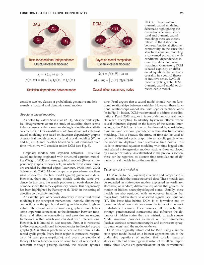
As noted by Valdes-Sosa et al. (2011), ‘‘despite philosoph-ical disagreements about the study of causality, there seemsto be a consensus that causal modeling is a legitimate statisti-cal enterprise.’’ One can differentiate two streams of statisticalcausal modeling: one based on Bayesian dependency graphsor graphical models called structural causal modeling (Whiteand Lu, 2010), and the other based on causal influences overtime, which we will consider under DCM (see Fig. 5).

Graphical models and Bayesian networks. Structuralcausal modeling originated with structural equation model-ing (Wright, 1921) and uses graphical models (Bayesian de-pendency graphs or Bayes nets) in which direct causal linksare encoded by directed edges (Lauritzen, 1996; Pearl, 2000;Spirtes et al., 2000). Model comparison procedures are thenused to discover the best model (graph) given some data.However, there may be many models with the same evi-dence. In this case, the search produces an equivalence classof models with the same explanatory power. This degeneracyhas been highlighted by Ramsey et al. (2010) in the setting ofeffective connectivity analysis.

An essential part of network discovery in structural causalmodeling is the concept of intervention—namely, eliminatingconnections in the graph and setting certain nodes to givenvalues. The causal calculus based on graphical models hassome important connections to the distinction between func-tional and effective connectivity and provides an elegantframework within which one can deal with interventions.However, it is limited in two respects. First, it is restrictedto discovering conditional independencies in directed acyclicgraphs (DAG). This is problematic because the brain is a di-rected cyclic graph. Every brain region is connected recipro-cally (at least polysynaptically), and every computationaltheory of brain function rests on some form of reciprocal orreentrant message passing. Second, the calculus ignores

time. Pearl argues that a causal model should rest on func-tional relationships between variables. However, these func-tional relationships cannot deal with (cyclic) feedback loops(as in Fig. 3). In fact, DCM was invented to address these lim-itations. Pearl (2000) argues in favor of dynamic causal mod-els when attempting to identify hysteresis effects, wherecausal influences depend on the history of the system. Inter-estingly, the DAG restriction can be finessed by consideringdynamics and temporal precedence within structural causalmodeling. This is because the arrow of time can be used toconvert a directed cyclic graph into an acyclic graph whenthe nodes are deployed over successive time points. Thisleads to structural equation modeling with time-lagged dataand related autoregression models, such as those employedby Granger causality. As established in the previous section,these can be regarded as discrete time formulations of dy-namic causal models in continuous time.

Dynamic causal modeling

DCM refers to the (Bayesian) inversion and comparison ofdynamic models that cause observed data. These models canbe regarded as state-space models expressed as (ordinary,stochastic, or random) differential equations that govern themotion of hidden neurophysiological states. Usually, thesemodels are also equipped with an observer function thatmaps from hidden states to observed signals [see Equation(1)]. The basic idea behind DCM is to formulate one ormore models of how data are caused in terms of a networkof distributed sources. These sources talk to each otherthrough parameterized connections and influence the dy-namics of hidden states that are intrinsic to each source.Model inversion provides estimates of their parameters(such as extrinsic connection strengths and intrinsic or synap-tic parameters) and the model evidence.

DCM was originally introduced for fMRI using a simplestate-space model based on a bilinear approximation to theunderlying equations of motion that couple neuronalstates in different brain regions (Friston et al., 2003). Impor-tantly, these DCMs are generalizations of the conventional

FIG. 5. Structural anddynamic causal modeling.Schematic highlighting thedistinctions between struc-tural and dynamic causalmodeling; these are closelyrelated to the distinctionbetween functional effectiveconnectivity, in the sense thatstructural equation modelingis concerned principally withconditional dependencies in-duced by static nonlinearmappings. Conversely, DCMis based explicitly on differ-ential equations that embodycausality in a control theoryor intuitive sense. DAG, di-rected a cyclic graph; DCM,dynamic causal model or di-rected cyclic model.


convolution model used to analyze fMRI data. The only dif-ference is that one allows for hidden neuronal states in onepart of the brain to be influenced by neuronal states else-where. In this sense, they are biophysically informed multi-variate analyses of distributed brain responses.

Most DCMs consider point sources for fMRI,magnetoencephalography (MEG) and electroencephalography(EEG) data (c.f., equivalent current dipoles) and are formallyequivalent to the graphical models used in structural causalmodeling. However, in DCM, they are used as explicit gener-

ative models of observed responses. Inference on the couplingwithin and between nodes (brain regions) is generally based onperturbing the system and trying to explain the observed re-sponses by inverting the model. This inversion furnishes poste-rior or conditional probability distributions over unknownparameters (e.g., effective connectivity) and the model evi-dence for model comparison (Penny et al., 2004). The powerof Bayesian model comparison, in the context of DCM, has be-come increasingly evident. This now represents one of themost important applications of DCM and allows different

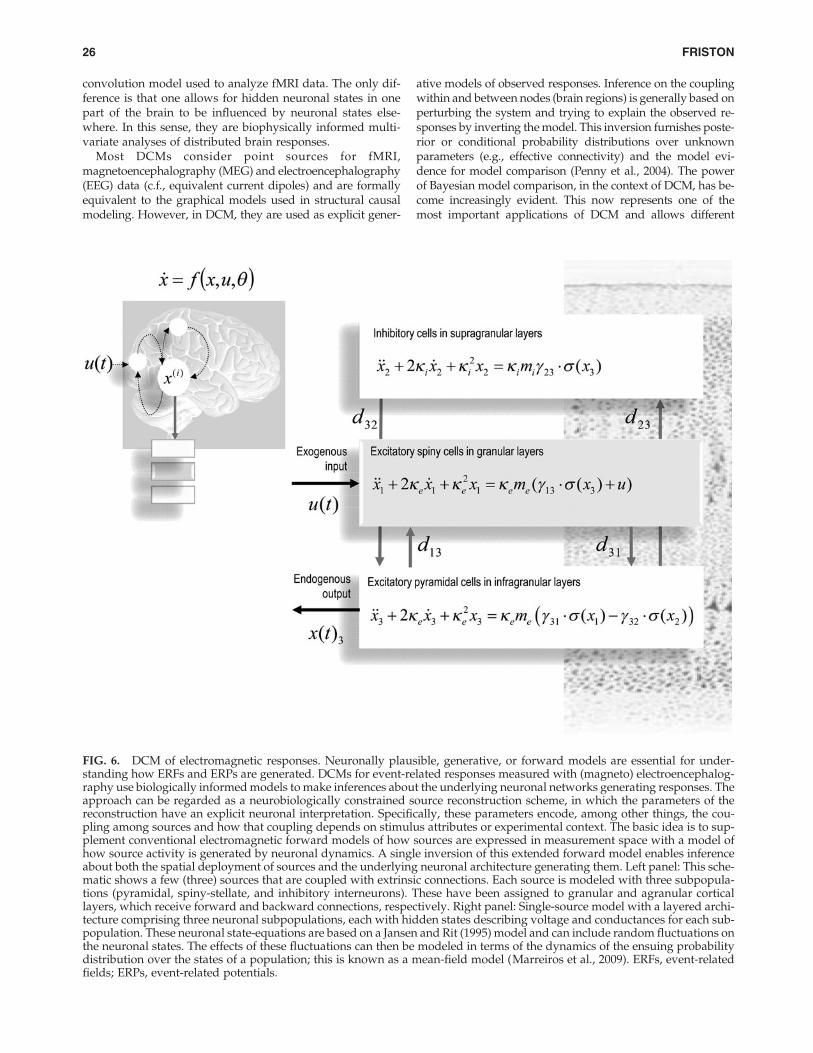
FIG. 6. DCM of electromagnetic responses. Neuronally plausible, generative, or forward models are essential for under-standing how ERFs and ERPs are generated. DCMs for event-related responses measured with (magneto) electroencephalog-raphy use biologically informed models to make inferences about the underlying neuronal networks generating responses. Theapproach can be regarded as a neurobiologically constrained source reconstruction scheme, in which the parameters of thereconstruction have an explicit neuronal interpretation. Specifically, these parameters encode, among other things, the cou-pling among sources and how that coupling depends on stimulus attributes or experimental context. The basic idea is to sup-plement conventional electromagnetic forward models of how sources are expressed in measurement space with a model ofhow source activity is generated by neuronal dynamics. A single inversion of this extended forward model enables inferenceabout both the spatial deployment of sources and the underlying neuronal architecture generating them. Left panel: This sche-matic shows a few (three) sources that are coupled with extrinsic connections. Each source is modeled with three subpopula-tions (pyramidal, spiny-stellate, and inhibitory interneurons). These have been assigned to granular and agranular corticallayers, which receive forward and backward connections, respectively. Right panel: Single-source model with a layered archi-tecture comprising three neuronal subpopulations, each with hidden states describing voltage and conductances for each sub-population. These neuronal state-equations are based on a Jansen and Rit (1995) model and can include random fluctuations onthe neuronal states. The effects of these fluctuations can then be modeled in terms of the dynamics of the ensuing probabilitydistribution over the states of a population; this is known as a mean-field model (Marreiros et al., 2009). ERFs, event-relatedfields; ERPs, event-related potentials.

26 FRISTON

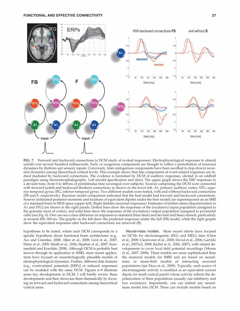
hypotheses to be tested, where each DCM corresponds to aspecific hypothesis about functional brain architectures (e.g.,Acs and Greenlee, 2008; Allen et al., 2008; Grol et al., 2007;Heim et al., 2009; Smith et al., 2006; Stephan et al., 2007; Sum-merfield and Koechlin, 2008). Although DCM is probably bestknown through its application to fMRI, more recent applica-tions have focused on neurobiologically plausible models ofelectrophysiological dynamics. Further, different data features(e.g., event-related potentials [ERPs] or induced responses)can be modeled with the same DCM. Figures 6–8 illustratesome key developments in DCM. I will briefly review thesedevelopments and then showcase them thematically by focus-ing on forward and backward connections among hierarchicalcortical areas.

Neural-mass models. More recent efforts have focusedon DCMs for electromagnetic (EEG and MEG) data (Chenet al., 2008; Clearwater et al., 2008; David et al., 2006; Garridoet al., 2007a,b, 2008; Kiebel et al., 2006, 2007), with related de-velopments to cover local field potential recordings (Moranet al., 2007, 2008). These models are more sophisticated thanthe neuronal models for fMRI and are based on neural-mass or mean-field models of interacting neuronalpopulations (see Deco et al., 2008). Typically, each source ofelectromagnetic activity is modeled as an equivalent currentdipole (or small cortical patch) whose activity reflects the de-polarization of three populations (usually one inhibitory andtwo excitatory). Importantly, one can embed any neural-mass model into DCM. These can include models based on

FIG. 7. Forward and backward connections (a DCM study of evoked responses). Electrophysiological responses to stimuliunfold over several hundred milliseconds. Early or exogenous components are thought to reflect a perturbation of neuronaldynamics by (bottom-up) sensory inputs. Conversely, later endogenous components have been ascribed to (top-down) recur-rent dynamics among hierarchical cortical levels. This example shows that late components of event-related responses are in-deed mediated by backward connections. The evidence is furnished by DCM of auditory responses, elicited in an oddballparadigm using electroencephalography. Left (model specification and data): The upper graph shows the ERP responses toa deviant tone, from 0 to 400 ms of peristimulus time (averaged over subjects). Sources comprising the DCM were connectedwith forward (solid) and backward (broken) connections as shown on the lower left. A1, primary auditory cortex; STG, supe-rior temporal gyrus; IFG, inferior temporal gyrus. Two different models were tested, with and without backward connections(FB and F, respectively). Bayesian model comparison indicated that the best model had forward and backward connections.Sources (estimated posterior moments and locations of equivalent dipoles under the best model) are superimposed on an MRIof a standard brain in MNI space (upper left). Right (hidden neuronal responses): Estimates of hidden states (depolarization inA1 and STG) are shown in the right panels. Dotted lines show the responses of the (excitatory) input population (assigned tothe granular layer of cortex), and solid lines show the responses of the (excitatory) output population (assigned to pyramidalcells) (see Fig. 6). One can see a clear difference in responses to standard (blue lines) and deviant (red lines) stimuli, particularlyat around 200–300 ms. The graphs on the left show the predicted responses under the full (FB) model, while the right graphsshow the equivalent responses after backward connections are removed (B).


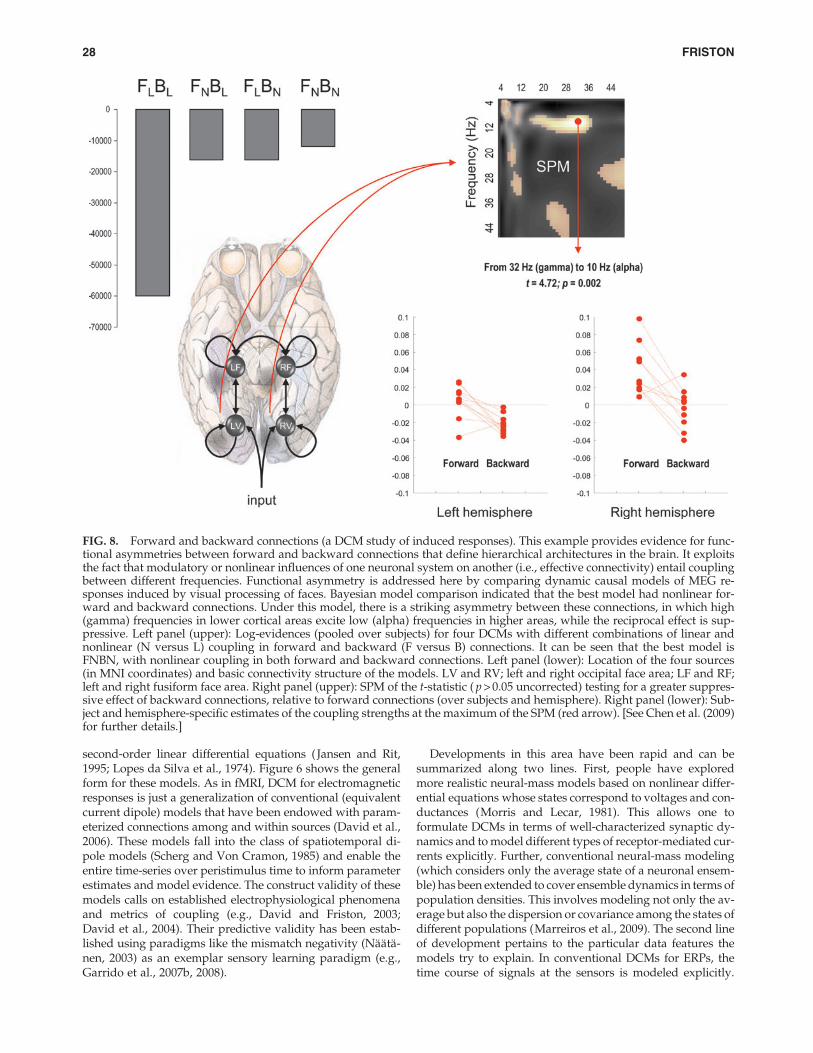
second-order linear differential equations ( Jansen and Rit,1995; Lopes da Silva et al., 1974). Figure 6 shows the generalform for these models. As in fMRI, DCM for electromagneticresponses is just a generalization of conventional (equivalentcurrent dipole) models that have been endowed with param-eterized connections among and within sources (David et al.,2006). These models fall into the class of spatiotemporal di-pole models (Scherg and Von Cramon, 1985) and enable theentire time-series over peristimulus time to inform parameterestimates and model evidence. The construct validity of thesemodels calls on established electrophysiological phenomenaand metrics of coupling (e.g., David and Friston, 2003;David et al., 2004). Their predictive validity has been estab-lished using paradigms like the mismatch negativity (Naata-nen, 2003) as an exemplar sensory learning paradigm (e.g.,Garrido et al., 2007b, 2008).

Developments in this area have been rapid and can besummarized along two lines. First, people have exploredmore realistic neural-mass models based on nonlinear differ-ential equations whose states correspond to voltages and con-ductances (Morris and Lecar, 1981). This allows one toformulate DCMs in terms of well-characterized synaptic dy-namics and to model different types of receptor-mediated cur-rents explicitly. Further, conventional neural-mass modeling(which considers only the average state of a neuronal ensem-ble) has been extended to cover ensemble dynamics in terms ofpopulation densities. This involves modeling not only the av-erage but also the dispersion or covariance among the states ofdifferent populations (Marreiros et al., 2009). The second lineof development pertains to the particular data features themodels try to explain. In conventional DCMs for ERPs, thetime course of signals at the sensors is modeled explicitly.

FIG. 8. Forward and backward connections (a DCM study of induced responses). This example provides evidence for func-tional asymmetries between forward and backward connections that define hierarchical architectures in the brain. It exploitsthe fact that modulatory or nonlinear influences of one neuronal system on another (i.e., effective connectivity) entail couplingbetween different frequencies. Functional asymmetry is addressed here by comparing dynamic causal models of MEG re-sponses induced by visual processing of faces. Bayesian model comparison indicated that the best model had nonlinear for-ward and backward connections. Under this model, there is a striking asymmetry between these connections, in which high(gamma) frequencies in lower cortical areas excite low (alpha) frequencies in higher areas, while the reciprocal effect is sup-pressive. Left panel (upper): Log-evidences (pooled over subjects) for four DCMs with different combinations of linear andnonlinear (N versus L) coupling in forward and backward (F versus B) connections. It can be seen that the best model isFNBN, with nonlinear coupling in both forward and backward connections. Left panel (lower): Location of the four sources(in MNI coordinates) and basic connectivity structure of the models. LV and RV; left and right occipital face area; LF and RF;left and right fusiform face area. Right panel (upper): SPM of the t-statistic ( p > 0.05 uncorrected) testing for a greater suppres-sive effect of backward connections, relative to forward connections (over subjects and hemisphere). Right panel (lower): Sub-ject and hemisphere-specific estimates of the coupling strengths at the maximum of the SPM (red arrow). [See Chen et al. (2009)for further details.]

28 FRISTON

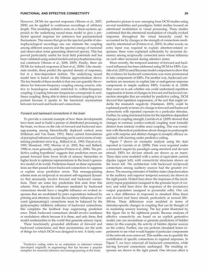
However, DCMs for spectral responses (Moran et al., 2007,2008) can be applied to continuous recordings of arbitrarylength. This modeling initiative rests on a linear-systems ap-proach to the underlying neural-mass model to give a pre-dicted spectral response for unknown but parameterizedfluctuations. This means that given the spectral profile of elec-trophysiological recordings one can estimate the couplingamong different sources and the spectral energy of neuronaland observation noise generating observed spectra. This hasproved particularly useful for local field potentials and hasbeen validated using animal models and psychopharmacolog-ical constructs (Moran et al., 2008, 2009). Finally, there areDCMs for induced responses (Chen et al., 2008). Like steady-state models, these predict the spectral density of responses,but in a time-dependent fashion. The underlying neuralmodel here is based on the bilinear approximation above.The key benefit of these models is that one can quantify the ev-idence for between-frequency coupling among sources, rela-tive to homologous models restricted to within-frequencycoupling. Coupling between frequencies corresponds to non-linear coupling. Being able to detect nonlinear coupling is im-portant because it speaks to the functional asymmetriesbetween forward and backward connections.

Forward and backward connections in the brain

To provide a concrete example of how these developmentshave been used to build a picture of distributed processing inthe brain, we focus on the role of forward and backward mes-sage-passing among hierarchically deployed cortical areas(Felleman and Van Essen, 1991). Many current formulationsof perceptual inference and learning can be cast in terms of min-imizing prediction error (e.g., Ballard et al., 1983; Dayan et al.,1995; Mumford, 1992; Murray et al., 2002; Rao and Ballard,1998) or, more generally, surprise (Friston et al., 2006). The pre-dictive coding hypothesis{ suggests that prediction errors arepassed forward from lower levels of sensory hierarchies tohigher levels to optimize representations in the brain’s genera-tive model of its world. Predictions based on these representa-tions are then passed down backward connections to suppressor explain away prediction errors. This message-passingscheme rests on reciprocal or recurrent self-organized dynam-ics that necessarily involve forward and backward connec-tions. There are some key predictions that arise from thisscheme. First, top-down influences mediated by backwardconnections should have a tangible influence on evoked re-sponses that are modulated by prior expectations induced bypriming and attention. Second, the excitatory influences of for-ward (glutamatergic) connections must be balanced by the(polysynaptic) inhibitory influence of backward connections;this completes the feedback loop suppressing predictionerror. Third, backward connections should involve nonlinearor modulatory effects because it is these, and only these, thatmodel nonlinearities in the world that generate sensory input.

These functionally grounded attributes of forward andbackward connections, and their asymmetries, are the sortsof things for which DCM was designed to test. A fairly com-

prehensive picture is now emerging from DCM studies usingseveral modalities and paradigms: Initial studies focused onattentional modulation in visual processing. These studiesconfirmed that the attentional modulation of visually evokedresponses throughout the visual hierarchy could beaccounted for by changes in the strength of connections medi-ated by attentional set (Friston et al., 2003). In other words, noextra input was required to explain attention-related re-sponses; these were explained sufficiently by recurrent dy-namics among reciprocally connected areas whose influenceon each other increased during attentive states.

More recently, the temporal anatomy of forward and back-ward influences has been addressed using DCM for ERPs. Gar-rido et al. (2007a) used Bayesian model comparison to show thatthe evidence for backward connections was more pronouncedin later components of ERPs. Put another way, backward con-nections are necessary to explain late or endogenous responsecomponents in simple auditory ERPs. Garrido et al. (2008)then went on to ask whether one could understand repetitionsuppression in terms of changes in forward and backward con-nection strengths that are entailed by predictive coding. DCMshowed that repetition suppression, of the sort that might un-derlie the mismatch negativity (Naatanen, 2003), could beexplained purely in terms of a change in forward and backwardconnections with repeated exposure to a particular stimulus.Further, by using functional forms for the repetition-dependentchanges in coupling strength, Garrido et al. (2009) showed thatchanges in extrinsic (cortico-cortical) coupling were formallydistinct from intrinsic (within area) coupling. This was consis-tent with theoretical predictions about changes in postsynapticgain with surprise and distinct changes in synaptic efficacy as-sociated with learning under predictive coding.

Figure 7 shows an exemplar analysis using the datareported in Garrido et al. (2008). Data were acquired undera mismatch negativity paradigm using standard and deviantstimuli. ERPs for deviant stimuli are shown as an insert.These data were modeled with a series of equivalent currentdipoles (upper left), with connectivity structures shown onthe lower left. The architecture with backward (reciprocal)connections among auditory sources had the greatest evi-dence. The ensuing estimates of hidden states (depolarizationin the auditory and superior temporal sources) are shown inthe right panels. Dotted lines show the responses of the (excit-atory) input population (assigned to the granular layer of cor-tex), and solid lines show the responses of the (excitatory)output population (assigned to pyramidal cells). One cansee a clear difference in responses to standard (blue lines)and deviant (red lines) stimuli, particularly at around 200–300 ms. These differences were modeled in terms ofstimulus-specific changes in coupling that can be thought ofas mediating sensory learning. The key point illustrated bythis figure lies in the rightmost panels. Because analyses ofeffective connectivity are based on an explicit generativemodel, one can reconstitute or generate predictions of hiddenstates (in this example, the activity of hidden dipolar sourceson the cortex). Further, one can perform simulated lesion ex-periments to see what would happen if particular componentsof the network were removed. This enables one to quantify thecontribution of specific connections to regional responses. InFigure 7, we have removed all backward connections, whileleaving forward connections unchanged. The resulting re-sponses are shown in the right panels. One obvious effect is

{Predictive coding refers to an estimation or inference scheme(developed originally in engineering) that has become a popularmetaphor for neuronal inference and message-passing in the brain.


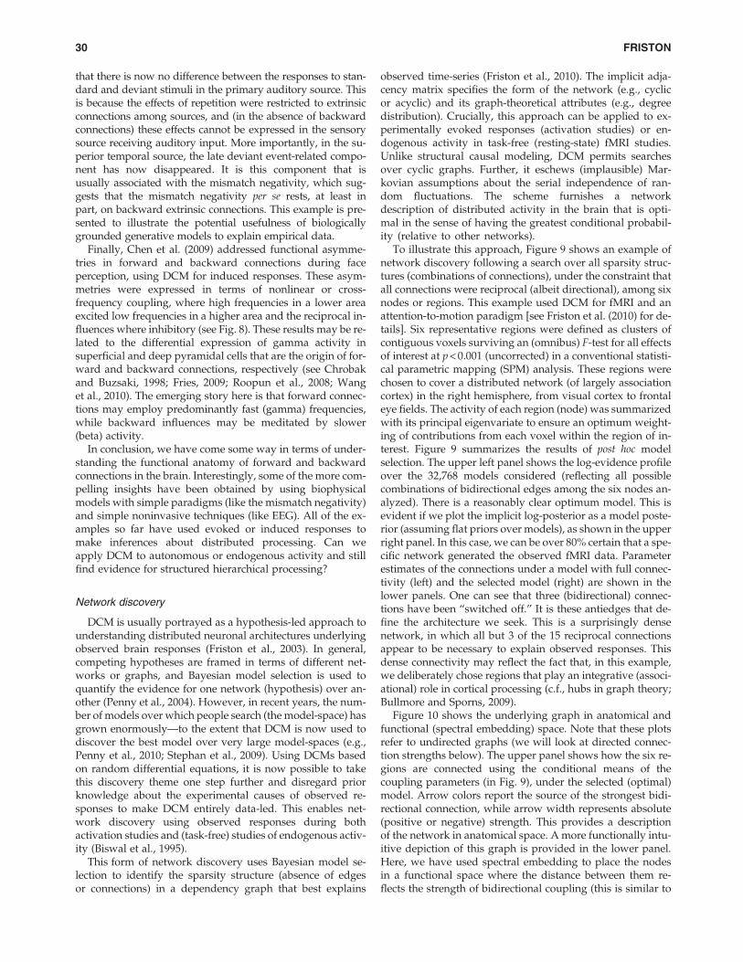
that there is now no difference between the responses to stan-dard and deviant stimuli in the primary auditory source. Thisis because the effects of repetition were restricted to extrinsicconnections among sources, and (in the absence of backwardconnections) these effects cannot be expressed in the sensorysource receiving auditory input. More importantly, in the su-perior temporal source, the late deviant event-related compo-nent has now disappeared. It is this component that isusually associated with the mismatch negativity, which sug-gests that the mismatch negativity per se rests, at least inpart, on backward extrinsic connections. This example is pre-sented to illustrate the potential usefulness of biologicallygrounded generative models to explain empirical data.

Finally, Chen et al. (2009) addressed functional asymme-tries in forward and backward connections during faceperception, using DCM for induced responses. These asym-metries were expressed in terms of nonlinear or cross-frequency coupling, where high frequencies in a lower areaexcited low frequencies in a higher area and the reciprocal in-fluences where inhibitory (see Fig. 8). These results may be re-lated to the differential expression of gamma activity insuperficial and deep pyramidal cells that are the origin of for-ward and backward connections, respectively (see Chrobakand Buzsaki, 1998; Fries, 2009; Roopun et al., 2008; Wanget al., 2010). The emerging story here is that forward connec-tions may employ predominantly fast (gamma) frequencies,while backward influences may be meditated by slower(beta) activity.

In conclusion, we have come some way in terms of under-standing the functional anatomy of forward and backwardconnections in the brain. Interestingly, some of the more com-pelling insights have been obtained by using biophysicalmodels with simple paradigms (like the mismatch negativity)and simple noninvasive techniques (like EEG). All of the ex-amples so far have used evoked or induced responses tomake inferences about distributed processing. Can weapply DCM to autonomous or endogenous activity and stillfind evidence for structured hierarchical processing?

Network discovery

DCM is usually portrayed as a hypothesis-led approach tounderstanding distributed neuronal architectures underlyingobserved brain responses (Friston et al., 2003). In general,competing hypotheses are framed in terms of different net-works or graphs, and Bayesian model selection is used toquantify the evidence for one network (hypothesis) over an-other (Penny et al., 2004). However, in recent years, the num-ber of models over which people search (the model-space) hasgrown enormously—to the extent that DCM is now used todiscover the best model over very large model-spaces (e.g.,Penny et al., 2010; Stephan et al., 2009). Using DCMs basedon random differential equations, it is now possible to takethis discovery theme one step further and disregard priorknowledge about the experimental causes of observed re-sponses to make DCM entirely data-led. This enables net-work discovery using observed responses during bothactivation studies and (task-free) studies of endogenous activ-ity (Biswal et al., 1995).

This form of network discovery uses Bayesian model se-lection to identify the sparsity structure (absence of edgesor connections) in a dependency graph that best explains

observed time-series (Friston et al., 2010). The implicit adja-cency matrix specifies the form of the network (e.g., cyclicor acyclic) and its graph-theoretical attributes (e.g., degreedistribution). Crucially, this approach can be applied to ex-perimentally evoked responses (activation studies) or en-dogenous activity in task-free (resting-state) fMRI studies.Unlike structural causal modeling, DCM permits searchesover cyclic graphs. Further, it eschews (implausible) Mar-kovian assumptions about the serial independence of ran-dom fluctuations. The scheme furnishes a networkdescription of distributed activity in the brain that is opti-mal in the sense of having the greatest conditional probabil-ity (relative to other networks).

To illustrate this approach, Figure 9 shows an example ofnetwork discovery following a search over all sparsity struc-tures (combinations of connections), under the constraint thatall connections were reciprocal (albeit directional), among sixnodes or regions. This example used DCM for fMRI and anattention-to-motion paradigm [see Friston et al. (2010) for de-tails]. Six representative regions were defined as clusters ofcontiguous voxels surviving an (omnibus) F-test for all effectsof interest at p < 0.001 (uncorrected) in a conventional statisti-cal parametric mapping (SPM) analysis. These regions werechosen to cover a distributed network (of largely associationcortex) in the right hemisphere, from visual cortex to frontaleye fields. The activity of each region (node) was summarizedwith its principal eigenvariate to ensure an optimum weight-ing of contributions from each voxel within the region of in-terest. Figure 9 summarizes the results of post hoc modelselection. The upper left panel shows the log-evidence profileover the 32,768 models considered (reflecting all possiblecombinations of bidirectional edges among the six nodes an-alyzed). There is a reasonably clear optimum model. This isevident if we plot the implicit log-posterior as a model poste-rior (assuming flat priors over models), as shown in the upperright panel. In this case, we can be over 80% certain that a spe-cific network generated the observed fMRI data. Parameterestimates of the connections under a model with full connec-tivity (left) and the selected model (right) are shown in thelower panels. One can see that three (bidirectional) connec-tions have been ‘‘switched off.’’ It is these antiedges that de-fine the architecture we seek. This is a surprisingly densenetwork, in which all but 3 of the 15 reciprocal connectionsappear to be necessary to explain observed responses. Thisdense connectivity may reflect the fact that, in this example,we deliberately chose regions that play an integrative (associ-ational) role in cortical processing (c.f., hubs in graph theory;Bullmore and Sporns, 2009).

Figure 10 shows the underlying graph in anatomical andfunctional (spectral embedding) space. Note that these plotsrefer to undirected graphs (we will look at directed connec-tion strengths below). The upper panel shows how the six re-gions are connected using the conditional means of thecoupling parameters (in Fig. 9), under the selected (optimal)model. Arrow colors report the source of the strongest bidi-rectional connection, while arrow width represents absolute(positive or negative) strength. This provides a descriptionof the network in anatomical space. A more functionally intu-itive depiction of this graph is provided in the lower panel.Here, we have used spectral embedding to place the nodesin a functional space where the distance between them re-flects the strength of bidirectional coupling (this is similar to

30 FRISTON

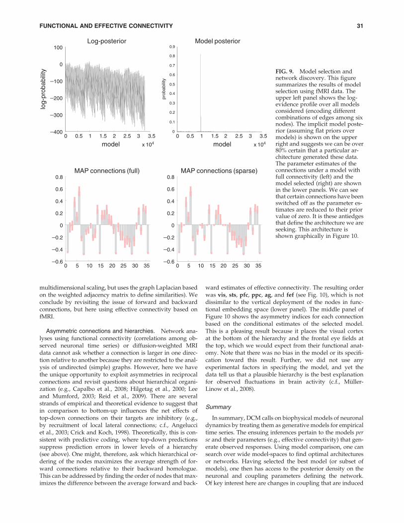
multidimensional scaling, but uses the graph Laplacian basedon the weighted adjacency matrix to define similarities). Weconclude by revisiting the issue of forward and backwardconnections, but here using effective connectivity based onfMRI.

Asymmetric connections and hierarchies. Network ana-lyses using functional connectivity (correlations among ob-served neuronal time series) or diffusion-weighted MRIdata cannot ask whether a connection is larger in one direc-tion relative to another because they are restricted to the anal-ysis of undirected (simple) graphs. However, here we havethe unique opportunity to exploit asymmetries in reciprocalconnections and revisit questions about hierarchical organi-zation (e.g., Capalbo et al., 2008; Hilgetag et al., 2000; Leeand Mumford, 2003; Reid et al., 2009). There are severalstrands of empirical and theoretical evidence to suggest thatin comparison to bottom-up influences the net effects oftop-down connections on their targets are inhibitory (e.g.,by recruitment of local lateral connections; c.f., Angelucciet al., 2003; Crick and Koch, 1998). Theoretically, this is con-sistent with predictive coding, where top-down predictionssuppress prediction errors in lower levels of a hierarchy(see above). One might, therefore, ask which hierarchical or-dering of the nodes maximizes the average strength of for-ward connections relative to their backward homologue.This can be addressed by finding the order of nodes that max-imizes the difference between the average forward and back-

ward estimates of effective connectivity. The resulting orderwas vis, sts, pfc, ppc, ag, and fef (see Fig. 10), which is notdissimilar to the vertical deployment of the nodes in func-tional embedding space (lower panel). The middle panel ofFigure 10 shows the asymmetry indices for each connectionbased on the conditional estimates of the selected model.This is a pleasing result because it places the visual cortexat the bottom of the hierarchy and the frontal eye fields atthe top, which we would expect from their functional anat-omy. Note that there was no bias in the model or its specifi-cation toward this result. Further, we did not use anyexperimental factors in specifying the model, and yet thedata tell us that a plausible hierarchy is the best explanationfor observed fluctuations in brain activity (c.f., Muller-Linow et al., 2008).

Summary

In summary, DCM calls on biophysical models of neuronaldynamics by treating them as generative models for empiricaltime series. The ensuing inferences pertain to the models perse and their parameters (e.g., effective connectivity) that gen-erate observed responses. Using model comparison, one cansearch over wide model-spaces to find optimal architecturesor networks. Having selected the best model (or subset ofmodels), one then has access to the posterior density on theneuronal and coupling parameters defining the network.Of key interest here are changes in coupling that are induced

0 0.5 1 1.5 2 2.5 3 3.5

x 104 x 104

-400

-300

-200

-100

0

100Log-posterior

model

log-

prob

abili

ty

0 0.5 1 1.5 2 2.5 3 3.50

0.1

0.2

0.3

0.4

0.5

0.6

0.7

0.8

0.9Model posterior

model

prob

abili

ty

0 5 10 15 20 25 30 35-0.6

-0.4

-0.2

0

0.2

0.4

0.6

0.8

-0.6

-0.4

-0.2

0

0.2

0.4

0.6

0.8MAP connections (full)

0 5 10 15 20 25 30 35

MAP connections (sparse)

FIG. 9. Model selection andnetwork discovery. This figuresummarizes the results of modelselection using fMRI data. Theupper left panel shows the log-evidence profile over all modelsconsidered (encoding differentcombinations of edges among sixnodes). The implicit model poste-rior (assuming flat priors overmodels) is shown on the upperright and suggests we can be over80% certain that a particular ar-chitecture generated these data.The parameter estimates of theconnections under a model withfull connectivity (left) and themodel selected (right) are shownin the lower panels. We can seethat certain connections have beenswitched off as the parameter es-timates are reduced to their priorvalue of zero. It is these antiedgesthat define the architecture we areseeking. This architecture isshown graphically in Figure 10.


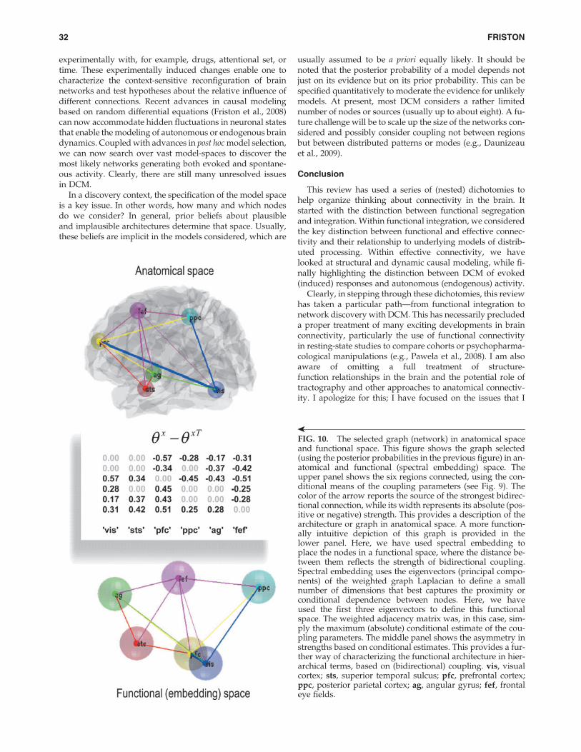
experimentally with, for example, drugs, attentional set, ortime. These experimentally induced changes enable one tocharacterize the context-sensitive reconfiguration of brainnetworks and test hypotheses about the relative influence ofdifferent connections. Recent advances in causal modelingbased on random differential equations (Friston et al., 2008)can now accommodate hidden fluctuations in neuronal statesthat enable the modeling of autonomous or endogenous braindynamics. Coupled with advances in post hoc model selection,we can now search over vast model-spaces to discover themost likely networks generating both evoked and spontane-ous activity. Clearly, there are still many unresolved issuesin DCM.

In a discovery context, the specification of the model spaceis a key issue. In other words, how many and which nodesdo we consider? In general, prior beliefs about plausibleand implausible architectures determine that space. Usually,these beliefs are implicit in the models considered, which are

usually assumed to be a priori equally likely. It should benoted that the posterior probability of a model depends notjust on its evidence but on its prior probability. This can bespecified quantitatively to moderate the evidence for unlikelymodels. At present, most DCM considers a rather limitednumber of nodes or sources (usually up to about eight). A fu-ture challenge will be to scale up the size of the networks con-sidered and possibly consider coupling not between regionsbut between distributed patterns or modes (e.g., Daunizeauet al., 2009).

Conclusion

This review has used a series of (nested) dichotomies tohelp organize thinking about connectivity in the brain. Itstarted with the distinction between functional segregationand integration. Within functional integration, we consideredthe key distinction between functional and effective connec-tivity and their relationship to underlying models of distrib-uted processing. Within effective connectivity, we havelooked at structural and dynamic causal modeling, while fi-nally highlighting the distinction between DCM of evoked(induced) responses and autonomous (endogenous) activity.

Clearly, in stepping through these dichotomies, this reviewhas taken a particular path—from functional integration tonetwork discovery with DCM. This has necessarily precludeda proper treatment of many exciting developments in brainconnectivity, particularly the use of functional connectivityin resting-state studies to compare cohorts or psychopharma-cological manipulations (e.g., Pawela et al., 2008). I am alsoaware of omitting a full treatment of structure-function relationships in the brain and the potential role oftractography and other approaches to anatomical connectiv-ity. I apologize for this; I have focused on the issues that I

FIG. 10. The selected graph (network) in anatomical spaceand functional space. This figure shows the graph selected(using the posterior probabilities in the previous figure) in an-atomical and functional (spectral embedding) space. Theupper panel shows the six regions connected, using the con-ditional means of the coupling parameters (see Fig. 9). Thecolor of the arrow reports the source of the strongest bidirec-tional connection, while its width represents its absolute (pos-itive or negative) strength. This provides a description of thearchitecture or graph in anatomical space. A more function-ally intuitive depiction of this graph is provided in thelower panel. Here, we have used spectral embedding toplace the nodes in a functional space, where the distance be-tween them reflects the strength of bidirectional coupling.Spectral embedding uses the eigenvectors (principal compo-nents) of the weighted graph Laplacian to define a smallnumber of dimensions that best captures the proximity orconditional dependence between nodes. Here, we haveused the first three eigenvectors to define this functionalspace. The weighted adjacency matrix was, in this case, sim-ply the maximum (absolute) conditional estimate of the cou-pling parameters. The middle panel shows the asymmetry instrengths based on conditional estimates. This provides a fur-ther way of characterizing the functional architecture in hier-archical terms, based on (bidirectional) coupling. vis, visualcortex; sts, superior temporal sulcus; pfc, prefrontal cortex;ppc, posterior parietal cortex; ag, angular gyrus; fef, frontaleye fields.

‰

32 FRISTON

am familiar with and believe hold the key to a mechanistic ap-plication of connectivity analyses in systems neuroscience. Ialso apologize if you have been pursuing Granger causalityor the comparison of correlations with gay abandon. I havebeen deliberately contrived in framing some of the conceptualissues to provoke a discussion. I may be wrong about theseissues, although I do not usually make mistakes. Havingsaid this, I did make a naive mistake in my first article onfunctional connectivity (Friston et al., 1993), which no onehas subsequently pointed out (perhaps out of kindness). Asubstantial part of Friston et al. (1993) was devoted to theproblem of identifying the eigenvectors of very large (voxel ·voxel) matrices, using a recursive (self-calling) algorithm.This was misguided and completely redundant becausethese eigenvectors can be accessed easily using singularvalue decomposition of the original (voxel · time) data ma-trix. I am grateful to Fred Brookstein for pointing this outafter seeing me present the original idea. I tell this story to re-mind myself that every journey of discovery has to beginsomewhere, and there is so much to learn (individually andcollectively). Given the trends in publications on brain con-nectivity (Fig. 1), one might guess that we have nowembarked on a journey; a journey that I am sure is takingus in the right direction. I would like to conclude by thankingthe editors of Brain Connectivity (Chris and Bharat) for askingme to write this review and helping shape its content. On be-half of their readers, I also wish them every success in theireditorial undertaking over the years to come.

Acknowledgments

This work was funded by the Wellcome Trust. I would liketo thank my colleagues on whose work this commentary isbased, including Michael Breakspear, Christian Buchel, C.C.Chen, Jean Daunizeau, Olivier David, Marta Garrido, LeeHarrison, Martin Havlicek, Maria Joao, Stefan Kiebel, Bao-juan Li, Andre Marreiros, Andreas Mechelli, RosalynMoran, Will Penny, Alard Roebroeck, Olaf Sporns, Klaas Ste-phan, Pedro Valdes-Sosa, and many others. I thank Klaas Ste-phan in particular for reading this article carefully andadvising on its content.

Author Disclosure Statement

No competing financial interests exist.

References

Abbott LF, Varela JA, Sen K, Nelson SB. 1997. Synaptic depres-sion and cortical gain control. Science 275:220–224.

Absher JR, Benson DF. 1993. Disconnection syndromes: an over-view of Geschwind’s contributions. Neurology 43:862–867.

Achard S, Salvador R, Whitcher B, Suckling J, Bullmore E. 2006. Aresilient, low-frequency, small-world human brain functionalnetwork with highly connected association cortical hubs. JNeurosci 26:63–72.

Acs F, Greenlee MW. 2008. Connectivity modulation of early vi-sual processing areas during covert and overt tracking tasks.Neuroimage 41:380–388.

Aertsen A, Preißl H. 1991. Dynamics of activity and connectivityin physiological neuronal networks. In: Schuster HG (ed.)Nonlinear Dynamics and Neuronal Networks. New York: VCHpublishers, Inc.; pp. 281–302.

Alexander DC. 2008. A general framework for experiment designin diffusion MRI and its application in measuring direct tis-sue-microstructure features. Magn Reson Med 60:439–448.

Allen P, Mechelli A, Stephan KE, Day F, Dalton J, Williams S,McGuire PK. 2008. Fronto-temporal interactions during overtverbal initiation and suppression. J Cogn Neurosci 20:1656–1669.

Alstott J, Breakspear M, Hagmann P, Cammoun L, Sporns O.2009. Modeling the impact of lesions in the human brain.PLoS Comput Biol 5:e1000408.

Baccala L, Sameshima K. 2001. Partial directed coherence: a new con-cept in neural structure determination. Biol Cybern 84:463–474.

Ballard DH, Hinton GE, Sejnowski TJ. 1983. Parallel visual com-putation. Nature 306:21–26.

Bassett DS, Bullmore ET. 2009. Human brain networks in healthand disease. Curr Opin Neurol 22:340–347.

Bassett DS, Meyer-Lindenberg A, Achard S, Duke T, Bullmore E.2006. Adaptive reconfiguration of fractal small-world humanbrain functional networks. Proc Natl Acad Sci U S A103:19518–19523.

Bedard C, Kroger H, Destexhe A. 2006. Model of low-pass filter-ing of local field potentials in brain tissue. Phys Rev E StatNonlin Soft Matter Phys 73(5 Pt 1):051911.

Behrens TE, Johansen-Berg H. 2005. Relating connectional archi-tecture to grey matter function using diffusion imaging.Philos Trans R Soc Lond B Biol Sci 360:903–911.

Bianciardi M, Fukunaga M, Van Gelderen P, Horovitz SG, DeZwart JA, Duyn JH. 2009. Modulation of spontaneous fMRIactivity in human visual cortex by behavioral state. Neuro-image 45:160–168.

Biswal B, Yetkin FZ, Haughton VM, Hyde JS. 1995. Functionalconnectivity in the motor cortex of resting human brainusing echo-planar MRI. Magn Reson Med 34:537–541.

Breakspear M, Stam CJ. 2005. Dynamics of a neural system with amultiscale architecture. Philos Trans R Soc Lond B Biol Sci360:1051–1074.

Bressler SL, Tognoli E. 2006. Operational principles of neurocog-nitive networks. Int J Psychophysiol 60:139–148.

Brodersen KH, Haiss F, Ong CS, Jung F, Tittgemeyer M, Buh-mann JM, Weber B, Stephan KE. (2011a). Model-based featureconstruction for multivariate decoding. Neuroimage (inpress); doi:10.1016/j.neuroimage.2010.04.036.

Brodersen KH, Schofield TM, Leff AP, Ong CS, Lomakina EI,Buhmann JM, Stephan KE (2011b). Generative embeddingfor model-based classification of fMRI data. Under review.

Buice MA, Cowan JD. 2009. Statistical mechanics of the neocor-tex. Prog Biophys Mol Biol 99:53–86.

Bullmore E, Sporns O. 2009. Complex brain networks: graph the-oretical analysis of structural and functional systems. Nat RevNeurosci 10:186–198.

Calhoun VD, Adali T. 2006. Unmixing fMRI with independentcomponent analysis. IEEE Eng Med Biol Mag 25:79–90.

Carr J. 1981. Applications of Centre Manifold Theory. Applied Math-ematical Sciences 35, Berlin-Heidelberg-New York: Springer-Verlag.

Chang C, Thomason M, Glover G. 2008. Mapping and correctionof vascular hemodynamic latency in the BOLD signal. Neuro-image 43:90–102.

Chen CC, Kiebel SJ, Friston KJ. 2008. Dynamic causal modellingof induced responses. Neuroimage 41:1293–1312.

Chen CC, Henson RN, Stephan KE, Kilner JM, Friston KJ. 2009.Forward and backward connections in the brain: a DCMstudy of functional asymmetries. Neuroimage 45:453–462.

Chrobak JJ, Buzsaki G. 1998. Gamma oscillations in the entorhi-nal cortex of the freely behaving rat. J Neurosci 18:388–398.


Clearwater JM, Kerr CC, Rennie CJ, Robinson PA. 2008. Neuralmechanisms of ERP change: combining insights from electro-physiology and mathematical modeling. J Integr Neurosci7:529–550.

Coombes S, Doole SH. 1996. Neuronal populations with recipro-cal inhibition and rebound currents: effects of synaptic andthreshold noise. Phys Rev E Stat Phys Plasmas Fluids RelatInterdiscip Top 54:4054–4065.

Craddock RC, Holtzheimer PE 3rd, Hu XP, Mayberg HS. 2009.Disease state prediction from resting state functional connec-tivity. Magn Reson Med 62:1619–1628.

Daunizeau J, Kiebel SJ, Friston KJ. 2009. Dynamic causal model-ling of distributed electromagnetic responses. Neuroimage47:590–601.

David O, Friston KJ. 2003. A neural-mass model for MEG/EEG:coupling and neuronal dynamics. Neuroimage 20:1743–1755.

David O, Cosmelli D, Friston KJ. 2004. Evaluation of differentmeasures of functional connectivity using a neural-massmodel. Neuroimage 21:659–673.

David O, Kiebel SJ, Harrison LM, Mattout J, Kilner JM, Friston KJ.2006. Dynamic causal modeling of evoked responses in EEGand MEG. Neuroimage 30:1255–1272.

David O, Guillemain I, Saillet S, Reyt S, Deransart C, Segebarth C,Depaulis A. 2008. Identifying neural drivers with functional MRI:an electrophysiological validation. PLoS Biology 6:2683–2697.

Dayan P, Hinton GE, Neal RM. 1995. The Helmholtz machine.Neural Comput 7:889–904.

Deco G, Jirsa VK, Robinson PA, Breakspear M, Friston K. 2008.The dynamic brain: from spiking neurons to neural-massesand cortical fields. PLoS Comput Biol 4:e1000092.

Deco G, Jirsa V, McIntosh AR, Sporns O, Kotter R. 2009. Key roleof coupling, delay, and noise in resting brain fluctuations.Proc Natl Acad Sci U S A 106:10302–10307.

Deco G, Jirsa VK, McIntosh AR. 2011. Emerging concepts for thedynamical organization of resting-state activity in the brain.Nat Rev Neurosci 12:43–56.

Deshpande G, Sathian K, Hu X. 2010. Assessing and compensat-ing for zero-lag correlation effects in time-lagged Grangercausality analysis of FMRI. IEEE Trans Biomed Eng 57:1446–1456.

Felleman DJ, Van Essen DC. 1991. Distributed hierarchical pro-cessing in the primate cerebral cortex. Cereb Cortex 1:1–47.

Fox M, Zhang D, Snyder A, Raichle M. 2009. The global signaland observed anticorrelated resting state brain networks.J Neurophysiol 101:3270–3283.

Freeman WJ. 1994. Characterization of state transitions in spa-tially distributed, chaotic, nonlinear, dynamical systems in ce-rebral cortex. Integr Physiol Behav Sci 29:294–306.

Freeman WJ. 2005. A field-theoretic approach to understandingscale-free neocortical dynamics. Biol Cybern 92:350–359.

Freyer F, Aquino K, Robinson PA, Ritter P, Breakspear M. 2009.Non-Gaussian statistics in temporal fluctuations of spontane-ous cortical activity. J Neurosci 29:8512–8524.

Fries P. 2009. Neuronal gamma-band synchronization as a funda-mental process in cortical computation. Annu Rev Neurosci32:209–224.

Friston K, Kilner J, Harrison L. 2006. A free-energy principle forthe brain. J Physiol Paris 100:70–87.

Friston KJ. 1995. Functional and effective connectivity in neuroi-maging: a synthesis. Hum Brain Mapp 2:56–78.

Friston KJ. 1998. Modes or models: a critique on independentcomponent analysis for fMRI. Trends Cogn Sci 2:373–375.

Friston KJ, Dolan RJ. 2010. Computational and dynamic modelsin neuroimaging. Neuroimage 52:752–765.

Friston KJ, Frith CD, Liddle PF, Frackowiak RS. 1993. Functionalconnectivity: the principal-component analysis of large (PET)data sets. J Cereb Blood Flow Metab 13:5–14.

Friston KJ, Ungerleider LG, Jezzard P, Turner R. 1995. Character-izing modulatory interactions between areas V1 and V2 inhuman cortex: a new treatment of functional MRI data.Hum Brain Mapp 2:211–224.

Friston KJ, Buchel C, Fink GR, Morris J, Rolls E, Dolan RJ. 1997.Psychophysiological and modulatory interactions in neuroi-maging. Neuroimage 6:218–229.

Friston KJ, Harrison L, Penny W. 2003. Dynamic causal model-ling. Neuroimage 19:1273–1302.

Friston KJ, Trujillo-Barreto N, Daunizeau J. 2008. DEM: a varia-tional treatment of dynamic systems. Neuroimage 41:849–885.

Friston KJ, Li B, Daunizeau J, Stephan KE. 2010. Network discov-ery with DCM. Neuroimage 56:1202–1221.

Garrido MI, Kilner JM, Kiebel SJ, Friston KJ. 2007a. Evoked brainresponses are generated by feedback loops. Proc Natl AcadSci U S A 104:20961–20966.

Garrido MI, Kilner JM, Kiebel SJ, Stephan KE, Friston KJ. 2007b.Dynamic causal modelling of evoked potentials: a reproduc-ibility study. Neuroimage 36:571–580.

Garrido MI, Friston KJ, Kiebel SJ, Stephan KE, Baldeweg T, KilnerJM. 2008. The functional anatomy of the MMN: a DCM studyof the roving paradigm. Neuroimage 42:936–944.

Garrido MI, Kilner JM, Kiebel SJ, Stephan KE, Baldeweg T, Fris-ton KJ. 2009. Repetition suppression and plasticity in thehuman brain. Neuroimage 48:269–279.

Gerstein GL, Perkel DH. 1969. Simultaneously recorded trains ofaction potentials: analysis and functional interpretation. Sci-ence 164:828–830.

Geweke JF. 1984. Measures of conditional linear dependence andfeedback between time series. J Am Stat Assoc 79:907–915.

Ghosh A, Rho Y, McIntosh AR, Kotter R, Jirsa VK. 2008. Corticalnetwork dynamics with time delays reveals functional con-nectivity in the resting brain. Cogn Neurodyn 2:115–120.

Ginzburg VL, Landau LD. 1950. On the theory of superconduc-tivity. Zh Eksp Teor Fiz 20:1064.

Goebel R, Roebroeck A, Kim D-S, Formisano E. 2003. Investigat-ing directed cortical interactions in time-resolved fMRI datausing vector autoregressive modeling and Granger causalitymapping. Magn Reson Imaging 21:1251–1261.

Goltz F. 1881. In: MacCormac W (ed.) Transactions of the 7th Inter-national Medical Congress. Vol. I. London: JW Kolkmann; pp.218–228.

Granger CWJ. 1969. Investigating causal relations by econometricmodels and cross-spectral methods. Econometrica 37:424–438.

Greicius MD, Supekar K, Menon V, Dougherty RF. 2009. Resting-state functional connectivity reflects structural connectivity inthe default mode network. Cereb Cortex 19:72–78.

Grol MY, Majdandzic J, Stephan KE, Verhagen L, DijkermanHC, Bekkering H, Verstraten FA, Toni I. 2007. Parieto-frontalconnectivity during visually guided grasping. J Neurosci 27:11877–11887.

Guye M, Bartolomei F, Ranjeva JP. 2008. Imaging structural andfunctional connectivity: towards a unified definition ofhuman brain organization? Curr Opin Neurol 21:393–403.

Haken H. 1983. Synergetics: An Introduction. Non-EquilibriumPhase Transition and Self-Organisation in Physics, Chemistryand Biology. 3rd Edition. Berlin-Heidelberg-New York:Springer-Verlag.

Harrison LM, Penny W, Friston KJ. 2003. Multivariate autore-gressive modeling of fMRI time series. Neuroimage 19:1477–1491.

34 FRISTON

Havlicek M, Jan J, Brazdil M, Calhoun VD. 2010. Dynamic Grangercausality based on Kalman filter for evaluation of functionalnetwork connectivity in fMRI data. Neuroimage 53:65–77.

Heim S, Eickhoff SB, Ischebeck AK, Friederici AD, Stephan KE,Amunts K. 2009. Effective connectivity of the left BA 44, BA45, and inferior temporal gyrus during lexical and phonologicaldecisions identified with DCM. Hum Brain Mapp 30:392–402.

Hesselmann G, Kell CA, Kleinschmidt A. 2008. Ongoing activityfluctuations in hMT + bias the perception of coherent visualmotion. J Neurosci 28:14481–14485.

Honey CJ, Kotter R, Breakspear M, Sporns O. 2007. Networkstructure of cerebral cortex shapes functional connectivityon multiple time scales. Proc Natl Acad Sci U S A104:10240–10245.

Honey CJ, Sporns O, Cammoun L, Gigandet X, Thiran JP, MeuliR, Hagmann P. 2009. Predicting human resting-state func-tional connectivity from structural connectivity. Proc NatlAcad Sci U S A 106:2035–2040.

Jansen BH, Rit VG. 1995. Electroencephalogram and visualevoked potential generation in a mathematical model of cou-pled cortical columns. Biol Cybern 73:357–366.

Jirsa VK, Haken H. 1996. Field theory of electromagnetic brain ac-tivity. Phys Rev Lett 77:960–963.

Jirsa VK, Kelso JA. 2000. Spatiotemporal pattern formation inneural systems with heterogeneous connection topologies.Phys Rev E Stat Phys Plasmas Fluids Relat Interdiscip Topics62(6 Pt B):8462–8465.

Jirsa VK, Friedrich R, Haken H, Kelso JA. 1994. A theoreticalmodel of phase transitions in the human brain. Biol Cybern71:27–35.

Kasahara M, Menon DK, Salmond CH, Outtrim JG, TaylorTavares JV, Carpenter TA, Pickard JD, Sahakian BJ, Stamata-kis EA. 2010. Altered functional connectivity in the motor net-work after traumatic brain injury. Neurology 75:168–176.

Kass RE, Raftery AE. 1995. Bayes factors. J Am Stat Assoc 90:773–795.

Kiebel SJ, David O, Friston KJ. 2006. Dynamic causal modellingof evoked responses in EEG/MEG with lead field parameter-ization. Neuroimage 30:1273–1284.

Kiebel SJ, Garrido MI, Friston KJ. 2007. Dynamic causal model-ling of evoked responses: the role of intrinsic connections.Neuroimage 36:332–345.

Kitzbichler MG, Smith ML, Christensen SR, Bullmore E. 2009.Broadband criticality of human brain network synchroniza-tion. PLoS Comput Biol 5:e1000314.

Kiviniemi V, Kantola J-H, Jauhiainen J, Hyvarinen A, TervonenO. 2003. Independent component analysis of nondeterministicfMRI signal sources. Neuroimage 19:253–260.

Kopell N, Ermentrout GB. 1986. Symmetry and phase-locking inchains of weakly coupled oscillators. Comm Pure Appl Math39:623–660.

Kriener B, Tetzlaff T, Aertsen A, Diesmann M, Rotter S. 2008.Correlations and population dynamics in cortical networks.Neural Comput 20:2185–2226.

Lauritzen S. 1996. Graphical Models. Oxford University Press:Oxford, UK.

Lee TS, Mumford D. 2003. Hierarchical Bayesian inference in thevisual cortex. J Opt Soc Am Opt Image Sci Vis 20:1434–1448.

Linkenkaer-Hansen K, Nikouline VV, Palva JM, Ilmoniemi RJ.2001. Long-range temporal correlations and scaling behaviorin human brain oscillations. J Neurosci 21:1370–1377.

Lopes da Silva FH, Hoeks A, Smits H, Zetterberg LH. 1974.Model of brain rhythmic activity. The alpha-rhythm of thethalamus. Kybernetik 15:27–37.

Marinazzo D, Liao W, Chen H. Stramaglia S. 2010. Nonlinearconnectivity by Granger causality. Neuroimage. [Epub aheadof print].

Marreiros AC, Kiebel SJ, Daunizeau J, Harrison LM, Friston KJ.2009. Population dynamics under the Laplace assumption.Neuroimage 44:701–714.

Marrelec G, Krainik A, Duffau H, Pelegrini-Issac M, Lehericy S,Doyon J, Benali H. 2006. Partial correlation for functionalbrain interactivity investigation in functional MRI. Neuro-image 32:228–237.

McIntosh AR, Gonzalez-Lima F. 1991. Structural modeling offunctional neural pathways mapped with 2-deoxyglucose: ef-fects of acoustic startle habituation on the auditory system.Brain Res 547:295–302.

McIntosh AR, Grady CL, Ungerleider LG, Haxby JV, RapoportSI, Horwitz B. 1994. Network analysis of cortical visual path-ways mapped with PET. J Neurosci 14:655–666.

McKeown MJ, Makeig S, Brown GG, Jung TP, Kindermann SS,Bell AJ, Sejnowski TJ. 1998. Analysis of fMRI data by blindseparation into independent spatial components. Hum BrainMapp 6:160–188.

Miller KJ, Sorensen LB, Ojemann JG, den Nijs M. 2009. ECoG ob-servations of power-law scaling in the human cortex. PLoSComput Biol 5:e1000609.

Moran RJ, Kiebel SJ, Stephan KE, Reilly RB, Daunizeau J, FristonKJ. 2007. A neural-mass model of spectral responses in elec-trophysiology. Neuroimage 37:706–720.

Moran RJ, Stephan KE, Kiebel SJ, Rombach N, O’Connor WT,Murphy KJ, Reilly RB, Friston KJ. 2008. Bayesian estimationof synaptic physiology from the spectral responses ofneural-masses. Neuroimage 42:272–284.

Moran RJ, Stephan KE, Seidenbecher T, Pape HC, Dolan RJ, Fris-ton KJ. 2009. Dynamic causal models of steady-state re-sponses. NeuroImage 44:796–811.

Morris C, Lecar H. 1981. Voltage oscillations in the barnacle giantmuscle fiber. Biophys J 35:193–213.

Muller-Linow M, Hilgetag CC, Hutt M-T. 2008. Organization ofexcitable dynamics in hierarchical biological networks. PLoSComput Biol 4:e1000190.

Mumford D. 1992. On the computational architecture of the neo-cortex. II. The role of cortico-cortical loops. Biol Cybern 66:241–251.

Murray SO, Kersten D, Olshausen BA, Schrater P, WoodsDL. 2002. Shape perception reduces activity in human pri-mary visual cortex. Proc Natl Acad Sci U S A 99:15164–15169.

Naatanen R. 2003. Mismatch negativity: clinical research andpossible applications. Int J Psychophysiol 48:179–188.

Nalatore H, Ding M, Rangarajan G. 2007. Mitigating the effectsof measurement noise on Granger causality. Phys Rev E 75:31123.1–31123.10.

Nolte G, Ziehe A, Nikulin V, Schlogl A, Kramer N, Brismar T,Muller K. 2008. Robustly estimating the flow direction of in-formation in complex physical systems. Phys Rev Lett100:234101.1–234101.4.

Patel R, Bowman F, Rilling J. 2006. A Bayesian approach to deter-mining connectivity of the human brain. Hum Brain Mapp27:267–276.

Pawela CP, Biswal BB, Cho YR, Kao DS, Li R, Jones SR, SchulteML, Matloub HS, Hudetz AG, Hyde JS. 2008. Resting-statefunctional connectivity of the rat brain. Magn Reson Med59:1021–1029.

Pearl J. 2000. Causality: Models, Reasoning and Inference. Cam-bridge University Press: Cambridge, UK.


Penny WD, Stephan KE, Mechelli A, Friston KJ. 2004. Comparingdynamic causal models. Neuroimage 22:1157–1172.

Phillips CG, Zeki S, Barlow HB. 1984. Localisation of functionin the cerebral cortex past present and future. Brain 107:327–361.

Protzner AB, McIntosh AR. 2006. Testing effective connectivitychanges with structural equation modeling: what does abad model tell us? Hum Brain Mapp 27:935–947.

Raichle ME, MacLeod AM, Snyder AZ, Powers WJ, Gusnard DA,Shulman GL. 2001. A default mode of brain function. ProcNatl Acad Sci U S A 98:676–682.

Ramsey JD, Hanson SJ, Hanson C, Halchenko YO, Poldrack RA,Glymour C. 2010. Six problems for causal inference fromfMRI. Neuroimage 49:1545–1558.

Rao RP, Ballard DH. 1998. Predictive coding in the visual cortex:a functional interpretation of some extra-classical receptivefield effects. Nat Neurosci 2:79–87.

Robinson PA, Rennie CJ, Wright JJ. 1997. Propagation and stabil-ity of waves of electrical activity in the cerebral cortex. PhysRev E 56:826–840.

Roebroeck A, Formisano E, Goebel R. 2005. Mapping directed in-fluence over the brain using Granger causality and fMRI.Neuroimage 25:230–242.

Roebroeck A, Formisano E, Goebel R. 2009. The identification ofinteracting networks in the brain using fMRI: model selection,causality and deconvolution. Neuroimage Sep 25. [Epubahead of print].

Rogers BP, Katwal SB, Morgan VL, Asplund CL, Gore JC. 2010.Functional MRI and multivariate autoregressive models.Magn Reson Imaging 28:1058–1065.

Roopun AK, Kramer MA, Carracedo LM, Kaiser M, Davies CH,Traub RD, Kopell NJ, Whittington MA. 2008. Period concate-nation underlies interactions between gamma and betarhythms in neocortex. Front Cell Neurosci 2:1.

Rubinov M, Sporns O, van Leeuwen C, Breakspear M. 2009. Sym-biotic relationship between brain structure and dynamics.BMC Neurosci 10:55.

Saneyoshi T, Fortin DA, Soderling TR. 2010. Regulation of spineand synapse formation by activity-dependent intracellularsignaling pathways. Curr Opin Neurobiol 20:108–115.

Scherg M, Von Cramon D. 1985. Two bilateral sources of the lateAEP as identified by a spatio-temporal dipole model. Electro-encephalogr Clin Neurophysiol 62:32–44.

Smith AP, Stephan KE, Rugg MD, Dolan RJ. 2006. Task and con-tent modulate amygdala-hippocampal connectivity in emo-tional retrieval. Neuron 49:631–638.

Smith SM, Miller KL, Salimi-Khorshidi G, Webster M, BeckmannCF, Nichols TE, Woolrich M. 2010. Network Modelling Meth-ods for FMRI. Neuroimage 54:875–891.

Spearman C. 1904. The proof and measurement of association be-tween two things. Am J Psychol 15:72–101.

Spirtes P, Glymour C, Scheines R. 1993. Causation, Prediction, andSearch. Berlin-Heidelberg-New York: Springer-Verlag.

Sporns O. 2007. Brain connectivity. Scholarpedia 2:4695.Sporns O. 2010. Networks of the Brain. Boston: MIT Press. ISBN-13:

978–0-262–01469-4.Sporns O, Tononi G, Kotter R. 2005. The human connectome: a

structural description of the human brain. PLoS ComputBiol 1:e42.

Stam CJ, de Bruin EA. 2004. Scale-free dynamics of global functionalconnectivity in the human brain. Hum Brain Mapp 22:97–109.

Staum M. 1995. Physiognomy and phrenology at the Paris Athe-nee. J Hist Ideas 56:443–462.

Stephan KE, Weiskopf N, Drysdale PM, Robinson PA, Friston KJ.2007. Comparing hemodynamic models with DCM. Neuro-image 38:387–401.

Stephan KE, Kasper L, Harrison LM, Daunizeau J, den OudenHE, Breakspear M, Friston KJ. 2008. Nonlinear dynamiccausal models for fMRI. Neuroimage 42:649–662.

Stephan KE, Tittgemeyer M, Knosche TR, Moran RJ, Friston KJ.2009. Tractography-based priors for dynamic causal models.Neuroimage 47:1628–1638.

Summerfield C, Koechlin E. 2008. A neural representation of priorinformation during perceptual inference. Neuron 59:336–347.

Tiao G, Wei W. 1976. Effect of temporal aggregation on the dy-namic relationship of two time series variables. Biometrika63:513–523.

Tognoli E, Kelso JA. 2009. Brain coordination dynamics: true andfalse faces of phase synchrony and metastability. Prog Neuro-biol 87:31–40.

Touboul J, Destexhe A. 2009. Can power-law scaling and neuro-nal avalanches arise from stochastic dynamics? PLoS One5:e8982.

Tschacher W, Haken H. 2007. Intentionality in non-equilibriumsystems? The functional aspects of self-organised pattern for-mation. New Ideas Psychol 25:1–15.

Tsuda I. 2001. Toward an interpretation of dynamic neural activ-ity in terms of chaotic dynamical systems. Behav Brain Sci24:793–810.

Valdes-Sosa PA, Roebroeck A, Daunizeau J, Friston K. 2011.Effective connectivity: influence, causality and biophysicalmodeling. Neuroimage Apr 5. [Epub a head of print].

Van Dijk KR, Hedden T, Venkataraman A, Evans KC, Lazar SW,Buckner RL. 2010. Intrinsic functional connectivity as a toolfor human connectomics: theory, properties, and optimiza-tion. J Neurophysiol 103:297–321.

Wang XJ. 2010. Physiological and computational principles ofcortical rhythms in cognition. Physiol Rev 90:1195–1268.

Wei W. 1978. The effect of temporal aggregation on parame-ter estimation in distributed lag model. J Econometrics 8:237–246.

White H, Lu X. 2010. Granger causality and dynamic structuralsystems. J Financial Econometrics 8:193–243.

Wolf ME, Mangiavacchi S, Sun X. 2003. Mechanisms by whichdopamine receptors may influence synaptic plasticity. AnnN Y Acad Sci 1003:241–249.

Wright S. 1921. Correlation and causation. J Agric Res 20:557–585.

Zhang H, Alexander DC. 2010. Axon diameter mapping in thepresence of orientation dispersion with diffusion MRI. MedImage Comput Comput Assist Interv 13:640–647.

Address correspondence to:Karl J. Friston

The Wellcome Trust Centre for NeuroimagingInstitute of Neurology

12 Queen SquareLondon WC1N 3BG

United Kingdom

E-mail: [email protected]

36 FRISTON

Documents

Functional and Effective Connectivity: A Reviekarl/Functional and Effective Connectivity A... · Functional and Effective Connectivity: A Review ... his review of functional and effective