Embed Size (px)
Citation preview
FUNCTIONAL ANALYSIS
AND
OPERATOR ALGEBRAS:
An Introduction
John M. Erdman
Portland State University
Version October 4, 2015
E-mail address: [email protected]
This work is licensed under the Creative Commons Attribution-ShareAlike 4.0 InternationalLicense. To view a copy of this license, visit http://creativecommons.org/licenses/by-sa/4.0/.
It is not essential for the value of an education that every idea be understood at thetime of its accession. Any person with a genuine intellectual interest and a wealthof intellectual content acquires much that he only gradually comes to understandfully in the light of its correlation with other related ideas. . . . Scholarship is aprogressive process, and it is the art of so connecting and recombining individualitems of learning by the force of one’s whole character and experience that nothingis left in isolation, and each idea becomes a commentary on many others.
- NORBERT WIENER

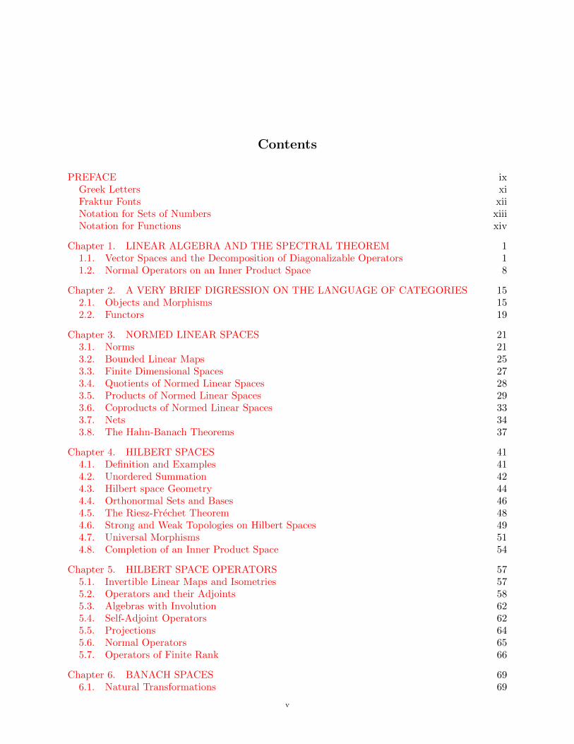
Contents
PREFACE ixGreek Letters xiFraktur Fonts xiiNotation for Sets of Numbers xiiiNotation for Functions xiv
Chapter 1. LINEAR ALGEBRA AND THE SPECTRAL THEOREM 11.1. Vector Spaces and the Decomposition of Diagonalizable Operators 11.2. Normal Operators on an Inner Product Space 8
Chapter 2. A VERY BRIEF DIGRESSION ON THE LANGUAGE OF CATEGORIES 152.1. Objects and Morphisms 152.2. Functors 19
Chapter 3. NORMED LINEAR SPACES 213.1. Norms 213.2. Bounded Linear Maps 253.3. Finite Dimensional Spaces 273.4. Quotients of Normed Linear Spaces 283.5. Products of Normed Linear Spaces 293.6. Coproducts of Normed Linear Spaces 333.7. Nets 343.8. The Hahn-Banach Theorems 37
Chapter 4. HILBERT SPACES 414.1. Definition and Examples 414.2. Unordered Summation 424.3. Hilbert space Geometry 444.4. Orthonormal Sets and Bases 464.5. The Riesz-Frechet Theorem 484.6. Strong and Weak Topologies on Hilbert Spaces 494.7. Universal Morphisms 514.8. Completion of an Inner Product Space 54
Chapter 5. HILBERT SPACE OPERATORS 575.1. Invertible Linear Maps and Isometries 575.2. Operators and their Adjoints 585.3. Algebras with Involution 625.4. Self-Adjoint Operators 625.5. Projections 645.6. Normal Operators 655.7. Operators of Finite Rank 66
Chapter 6. BANACH SPACES 696.1. Natural Transformations 69
v
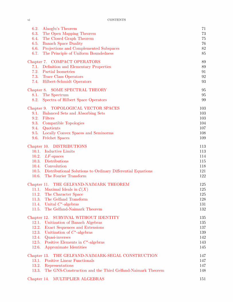
vi CONTENTS
6.2. Alaoglu’s Theorem 716.3. The Open Mapping Theorem 736.4. The Closed Graph Theorem 756.5. Banach Space Duality 766.6. Projections and Complemented Subspaces 826.7. The Principle of Uniform Boundedness 85
Chapter 7. COMPACT OPERATORS 897.1. Definition and Elementary Properties 897.2. Partial Isometries 917.3. Trace Class Operators 927.4. Hilbert-Schmidt Operators 93
Chapter 8. SOME SPECTRAL THEORY 958.1. The Spectrum 958.2. Spectra of Hilbert Space Operators 99
Chapter 9. TOPOLOGICAL VECTOR SPACES 1039.1. Balanced Sets and Absorbing Sets 1039.2. Filters 1039.3. Compatible Topologies 1049.4. Quotients 1079.5. Locally Convex Spaces and Seminorms 1089.6. Frechet Spaces 109
Chapter 10. DISTRIBUTIONS 11310.1. Inductive Limits 11310.2. LF -spaces 11410.3. Distributions 11510.4. Convolution 11810.5. Distributional Solutions to Ordinary Differential Equations 12110.6. The Fourier Transform 122
Chapter 11. THE GELFAND-NAIMARK THEOREM 12511.1. Maximal Ideals in C(X) 12511.2. The Character Space 12511.3. The Gelfand Transform 12811.4. Unital C∗-algebras 13111.5. The Gelfand-Naimark Theorem 132
Chapter 12. SURVIVAL WITHOUT IDENTITY 13512.1. Unitization of Banach Algebras 13512.2. Exact Sequences and Extensions 13712.3. Unitization of C∗-algebras 13912.4. Quasi-inverses 14212.5. Positive Elements in C∗-algebras 14312.6. Approximate Identities 145
Chapter 13. THE GELFAND-NAIMARK-SEGAL CONSTRUCTION 14713.1. Positive Linear Functionals 14713.2. Representations 14713.3. The GNS-Construction and the Third Gelfand-Naimark Theorem 148
Chapter 14. MULTIPLIER ALGEBRAS 151
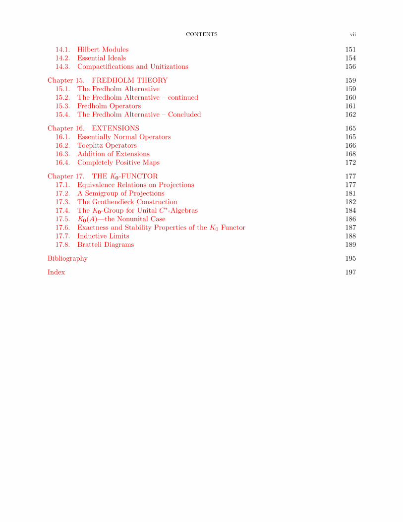
CONTENTS vii
14.1. Hilbert Modules 15114.2. Essential Ideals 15414.3. Compactifications and Unitizations 156
Chapter 15. FREDHOLM THEORY 15915.1. The Fredholm Alternative 15915.2. The Fredholm Alternative – continued 16015.3. Fredholm Operators 16115.4. The Fredholm Alternative – Concluded 162
Chapter 16. EXTENSIONS 16516.1. Essentially Normal Operators 16516.2. Toeplitz Operators 16616.3. Addition of Extensions 16816.4. Completely Positive Maps 172
Chapter 17. THE K0-FUNCTOR 17717.1. Equivalence Relations on Projections 17717.2. A Semigroup of Projections 18117.3. The Grothendieck Construction 18217.4. The K0-Group for Unital C∗-Algebras 18417.5. K0(A)—the Nonunital Case 18617.6. Exactness and Stability Properties of the K0 Functor 18717.7. Inductive Limits 18817.8. Bratteli Diagrams 189
Bibliography 195
Index 197

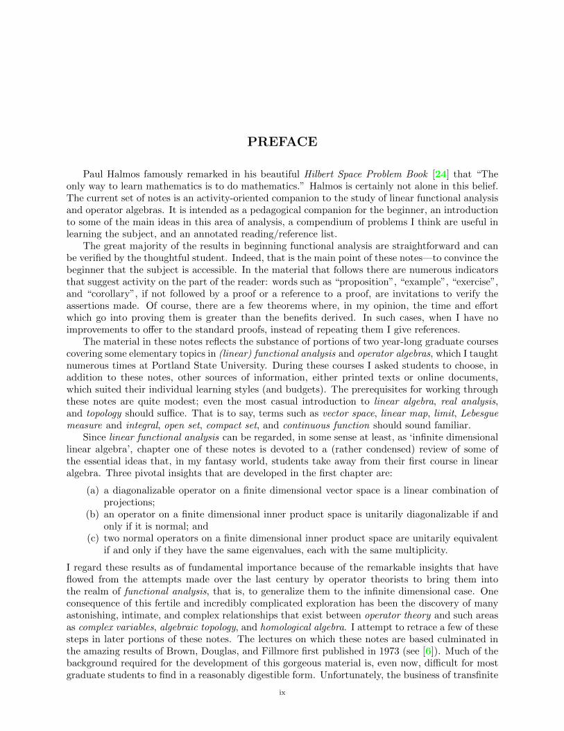
PREFACE
Paul Halmos famously remarked in his beautiful Hilbert Space Problem Book [24] that “Theonly way to learn mathematics is to do mathematics.” Halmos is certainly not alone in this belief.The current set of notes is an activity-oriented companion to the study of linear functional analysisand operator algebras. It is intended as a pedagogical companion for the beginner, an introductionto some of the main ideas in this area of analysis, a compendium of problems I think are useful inlearning the subject, and an annotated reading/reference list.
The great majority of the results in beginning functional analysis are straightforward and canbe verified by the thoughtful student. Indeed, that is the main point of these notes—to convince thebeginner that the subject is accessible. In the material that follows there are numerous indicatorsthat suggest activity on the part of the reader: words such as “proposition”, “example”, “exercise”,and “corollary”, if not followed by a proof or a reference to a proof, are invitations to verify theassertions made. Of course, there are a few theorems where, in my opinion, the time and effortwhich go into proving them is greater than the benefits derived. In such cases, when I have noimprovements to offer to the standard proofs, instead of repeating them I give references.
The material in these notes reflects the substance of portions of two year-long graduate coursescovering some elementary topics in (linear) functional analysis and operator algebras, which I taughtnumerous times at Portland State University. During these courses I asked students to choose, inaddition to these notes, other sources of information, either printed texts or online documents,which suited their individual learning styles (and budgets). The prerequisites for working throughthese notes are quite modest; even the most casual introduction to linear algebra, real analysis,and topology should suffice. That is to say, terms such as vector space, linear map, limit, Lebesguemeasure and integral, open set, compact set, and continuous function should sound familiar.
Since linear functional analysis can be regarded, in some sense at least, as ‘infinite dimensionallinear algebra’, chapter one of these notes is devoted to a (rather condensed) review of some ofthe essential ideas that, in my fantasy world, students take away from their first course in linearalgebra. Three pivotal insights that are developed in the first chapter are:
(a) a diagonalizable operator on a finite dimensional vector space is a linear combination ofprojections;
(b) an operator on a finite dimensional inner product space is unitarily diagonalizable if andonly if it is normal; and
(c) two normal operators on a finite dimensional inner product space are unitarily equivalentif and only if they have the same eigenvalues, each with the same multiplicity.
I regard these results as of fundamental importance because of the remarkable insights that haveflowed from the attempts made over the last century by operator theorists to bring them intothe realm of functional analysis, that is, to generalize them to the infinite dimensional case. Oneconsequence of this fertile and incredibly complicated exploration has been the discovery of manyastonishing, intimate, and complex relationships that exist between operator theory and such areasas complex variables, algebraic topology, and homological algebra. I attempt to retrace a few of thesesteps in later portions of these notes. The lectures on which these notes are based culminated inthe amazing results of Brown, Douglas, and Fillmore first published in 1973 (see [6]). Much of thebackground required for the development of this gorgeous material is, even now, difficult for mostgraduate students to find in a reasonably digestible form. Unfortunately, the business of transfinite
ix
x PREFACE
arm-waving that works passably well in the lecture room translates very poorly indeed to paper orelectronic media. As a result, these notes are in a sadly unfinished state. I’m working on them;and conceivably someone will finish what I do not.
If the material on linear algebra in the first chapter seems too condensed, a somewhat moreleisurely and thorough account can be found in my online notes [17]. Similarly, supplementarybackground material in advanced calculous, metric and topological spaces, Lebesgue integrals, andthe like, can be found in very many places, including [15] and [16].
There are of course a number of advantages and disadvantages in consigning a document toelectronic life. One advantage is the rapidity with which links implement cross-references. Huntingabout in a book for lemma 3.14.8 can be time-consuming (especially when an author engages inthe entirely logical but utterly infuriating practice of numbering lemmas, propositions, theorems,corollaries, and so on, separately). A perhaps more substantial advantage is the ability to correcterrors, add missing bits, clarify opaque arguments, and remedy infelicities of style in a timelyfashion. The correlative disadvantage is that a reader returning to the web page after a short timemay find everything (pages, definitions, theorems, sections) numbered differently. (LATEX is anamazing tool.) I will change the date on the title page to inform the reader of the date of the lastnontrivial update (that is, one that affects numbers or cross-references).
The most serious disadvantage of electronic life is impermanence. In most cases when a webpage vanishes so, for all practical purposes, does the information it contains. For this reason (andthe fact that I want this material to be freely available to anyone who wants it) I am making use ofa “Share Alike” license from Creative Commons. It is my hope that anyone who finds this materialuseful will correct what is wrong, add what is missing, and improve what is clumsy. I will includethe LATEX source files on my website so that using the document, or parts of it, does not involveendless retyping. Concerning the text itself, please send corrections, suggestions, complaints, andother comments to the author at
GREEK LETTERS xi
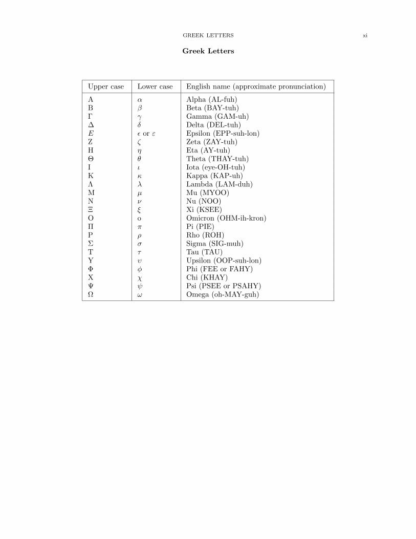
Greek Letters
Upper case Lower case English name (approximate pronunciation)
A α Alpha (AL-fuh)B β Beta (BAY-tuh)Γ γ Gamma (GAM-uh)∆ δ Delta (DEL-tuh)E ε or ε Epsilon (EPP-suh-lon)Z ζ Zeta (ZAY-tuh)H η Eta (AY-tuh)Θ θ Theta (THAY-tuh)I ι Iota (eye-OH-tuh)K κ Kappa (KAP-uh)Λ λ Lambda (LAM-duh)M µ Mu (MYOO)N ν Nu (NOO)Ξ ξ Xi (KSEE)O o Omicron (OHM-ih-kron)Π π Pi (PIE)P ρ Rho (ROH)Σ σ Sigma (SIG-muh)T τ Tau (TAU)Y υ Upsilon (OOP-suh-lon)Φ φ Phi (FEE or FAHY)X χ Chi (KHAY)Ψ ψ Psi (PSEE or PSAHY)Ω ω Omega (oh-MAY-guh)
xii PREFACE
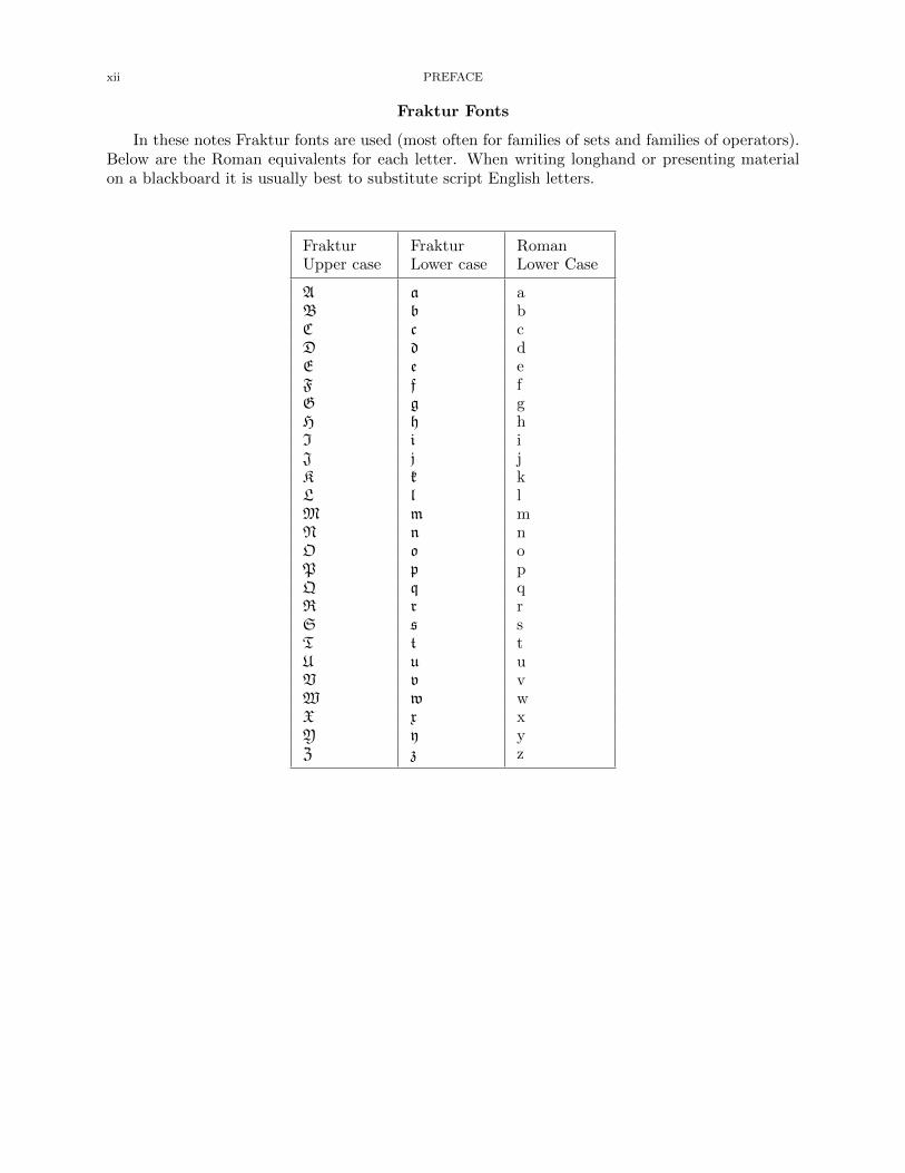
Fraktur Fonts
In these notes Fraktur fonts are used (most often for families of sets and families of operators).Below are the Roman equivalents for each letter. When writing longhand or presenting materialon a blackboard it is usually best to substitute script English letters.
Fraktur Fraktur RomanUpper case Lower case Lower Case
A a aB b bC c cD d dE e eF f fG g gH h hI i iJ j jK k kL l lM m mN n nO o oP p pQ q qR r rS s sT t tU u uV v vW w wX x xY y yZ z z
NOTATION FOR SETS OF NUMBERS xiii
Notation for Sets of Numbers
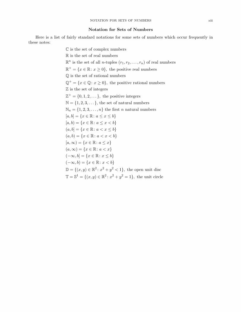
Here is a list of fairly standard notations for some sets of numbers which occur frequently inthese notes:
C is the set of complex numbers
R is the set of real numbers
Rn is the set of all n-tuples (r1, r2, . . . , rn) of real numbers
R+ = x ∈ R : x ≥ 0, the positive real numbers
Q is the set of rational numbers
Q+ = x ∈ Q : x ≥ 0, the positive rational numbers
Z is the set of integers
Z+ = 0, 1, 2, . . . , the positive integers
N = 1, 2, 3, . . . , the set of natural numbers
Nn = 1, 2, 3, . . . , n the first n natural numbers
[a, b] = x ∈ R : a ≤ x ≤ b[a, b) = x ∈ R : a ≤ x < b(a, b] = x ∈ R : a < x ≤ b(a, b) = x ∈ R : a < x < b[a,∞) = x ∈ R : a ≤ x(a,∞) = x ∈ R : a < x(−∞, b] = x ∈ R : x ≤ b(−∞, b) = x ∈ R : x < bD = (x, y) ∈ R2 : x2 + y2 < 1, the open unit disc
T = S1 = (x, y) ∈ R2 : x2 + y2 = 1, the unit circle
xiv PREFACE
Notation for Functions
Functions are familiar from beginning calculus. Informally, a function consists of a pair of setsand a “rule” which associates with each member of the first set (the domain) one and only onemember of the second (the codomain). While this informal “definition” is certainly adequate formost purposes and seldom leads to any misunderstanding, it is nevertheless sometimes useful tohave a more precise formulation. This is accomplished by defining a function in terms of a specialtype of relation between two sets.
A function f is an ordered triple (S, T,G) where S and T are sets and G is a subset of S×Tsatisfying:
(a) for each s ∈ S there is a t ∈ T such that (s, t) ∈ G, and(b) if (s, t1) and (s, t2) belong to G, then t1 = t2.
In this situation we say that f is a function from S into T (or that f maps S into T ) and writef : S → T . The set S is the domain (or the input space) of f . The set T is the codomain(or target space, or the output space) of f . And the relation G is the graph of f . In orderto avoid explicit reference to the graph G it is usual to replace the expression “(x, y) ∈ G ” by“y = f(x)”; the element f(x) is the image of x under f . In these notes (but not everywhere!) thewords “transformation”, “map”, and “mapping” are synonymous with “function”. The domain off is denoted by dom f .
If S and T are sets, then the family of all functions with domain S and codomain T is denotedby F(S, T ).
If f : S → T and A ⊆ S, then the restriction of f to A, denoted by f∣∣A
, is the mapping fromA into T whose value at each x in A is f(x).
If f : S → T and A ⊆ S, then f→(A), the image of A under f , is f(x) : x ∈ A. It is commonpractice to write f(A) for f→(A). The set f→(S) is the range (or image) of f ; usually we writeran f for f→(S).
If f : S → T and B ⊆ T , then f←(B), the inverse image of B under f , is x ∈ S : f(x) ∈ B.In many texts f←(B) is denoted by f−1(B). This notation may cause confusion by suggesting thatthe function f has an inverse when, in fact, it may not.
A function f : S → T is injective (or one-to-one) if f(x) = f(y) implies x = y for all x,y ∈ S. It is surjective (or onto) in for every t ∈ T there exists x ∈ S such that f(x) = t. Andit is bijective (or a one-to-one correspondence if it is both injective and surjective.
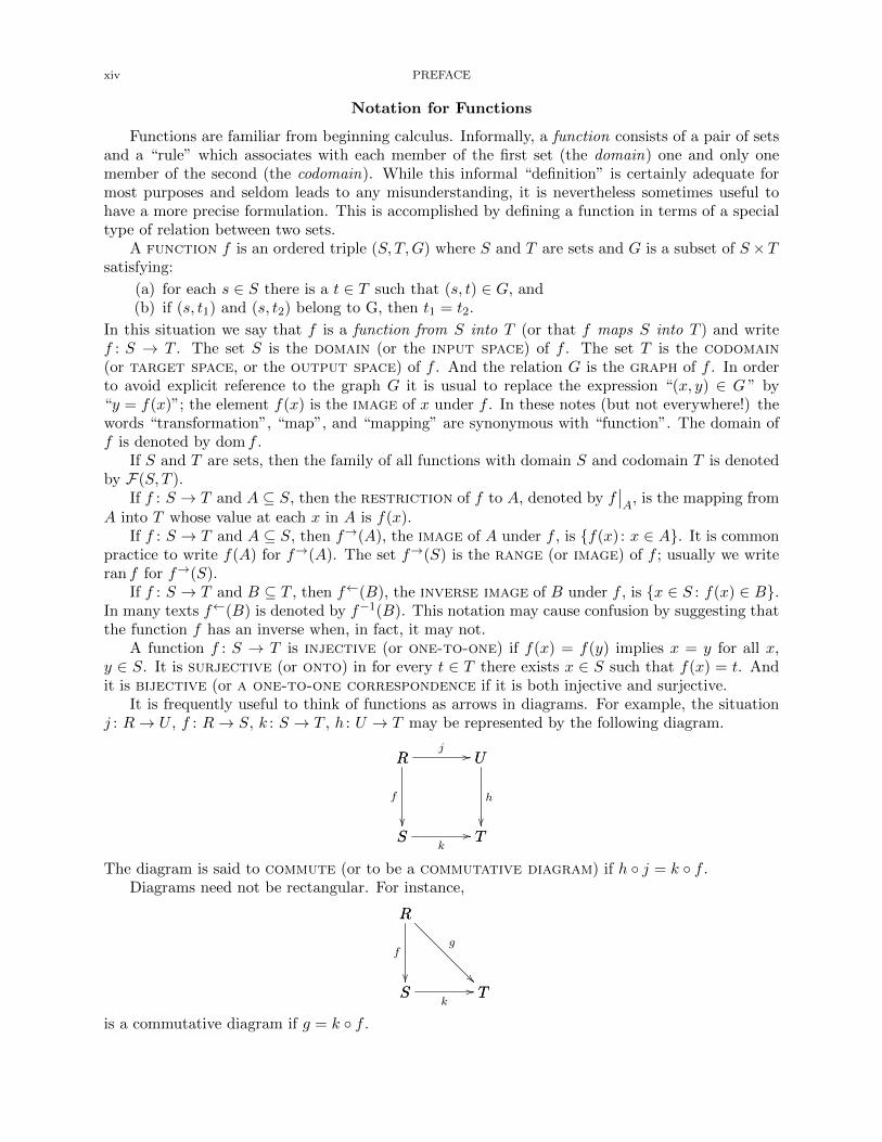
It is frequently useful to think of functions as arrows in diagrams. For example, the situationj : R→ U , f : R→ S, k : S → T , h : U → T may be represented by the following diagram.
S Tk
//
R
S
f
R Uj // U
T
h
The diagram is said to commute (or to be a commutative diagram) if h j = k f .Diagrams need not be rectangular. For instance,
S Tk
//
R
S
f
R
T
g
is a commutative diagram if g = k f .
CHAPTER 1
LINEAR ALGEBRA AND THE SPECTRAL THEOREM
The emphasis in beginning analysis courses is on the behavior of individual (real or complexvalued) functions. In a functional analysis course the focus is shifted to spaces of such functionsand certain classes of mappings between these spaces. It turns out that a concise, perhaps overlysimplistic, but certainly not misleading, description of such material is infinite dimensional linearalgebra. From an analyst’s point of view the greatest triumphs of linear algebra were, for themost part, theorems about operators on finite dimensional vector spaces (principally Rn and Cn).However, the vector spaces of scalar-valued mappings defined on various domains are typicallyinfinite dimensional. Whether one sees the process of generalizing the marvelous results of finitedimensional linear algebra to the infinite dimensional realm as a depressingly unpleasant string ofabstract complications or as a rich source of astonishing insights, fascinating new questions, andsuggestive hints towards applications in other fields depends entirely on one’s orientation towardsmathematics in general.
In light of the preceding remarks it may be helpful to begin our journey into this new terrainwith a brief review of some of the classical successes of linear algebra. It is not unusual for studentswho successfully complete a beginning linear algebra to have at the end only the vaguest idea ofwhat the course was about. Part of the blame for this may be laid on the many elementary textswhich make an unholy conflation of two quite different, if closely related subjects: the study ofvector spaces and the linear maps between them on the one hand, and inner product spaces andtheir linear maps on the other. Vector spaces have none of the geometric/topological notions ofdistance or length or perpendicularity or open set or angle between vectors; there is only additionand scalar multiplication. Inner product spaces are vector spaces endowed with these additionalstructures. Let’s look at them separately.
1.1. Vector Spaces and the Decomposition of Diagonalizable Operators
1.1.1. Convention. In these notes all vector spaces will be assumed to be vector spaces over thefield C of complex numbers (in which case it is called a complex vector space) or the field R of realnumbers (in which case it is a real vector space). No other fields will appear. When K appears itcan be taken to be either C or R. A scalar is a member of K; that is, either a complex numberor a real number.
1.1.2. Definition. The triple (V,+,M) is a vector space over K if (V,+) is an Abelian groupand M : K→ Hom(V ) is a unital ring homomorphism (where Hom(V ) is the ring of group homo-morphisms on V ).
To check on the meanings of any the terms in the preceding definition, take a look at the firstthree sections of the first chapter of my linear algebra notes [17].
1.1.3. Exercise. The definition of vector space found in many elementary texts is something likethe following: a vector space over K is a set V together with operations of addition and scalarmultiplication which satisfy the following axioms:
(1) if x, y ∈ V , then x+ y ∈ V ;(2) (x+ y) + z = x+ (y + z) for every x, y, z ∈ V (associativity);(3) there exists 0 ∈ V such that x+ 0 = x for every x ∈ V (existence of additive identity);(4) for every x ∈ V there exists −x ∈ V such that x+(−x) = 0 (existence of additive inverses);
1
2 1. LINEAR ALGEBRA AND THE SPECTRAL THEOREM
(5) x+ y = y + x for every x, y ∈ V (commutativity);(6) if α ∈ K and x ∈ V , then αx ∈ V ;(7) α(x+ y) = αx+ αy for every α ∈ K and every x, y ∈ V ;(8) (α+ β)x = αx+ βx for every α, β ∈ K and every x ∈ V ;(9) (αβ)x = α(βx) for every α, β ∈ K and every x ∈ V ; and
(10) 1x = x for every x ∈ V .
Verify that this definition is equivalent to the one given above in 1.1.2.
1.1.4. Definition. A subset M of a vector space V is a vector subspace of V if it is a vectorspace under the operations it inherits from V .
1.1.5. Proposition. A nonempty subset of M of a vector space V is a vector subspace of V if andonly if it is closed under addition and scalar multiplication. (That is: if x and y belong to M , sodoes x + y; and if x belongs to M and α ∈ K, then αx belongs to M .)
1.1.6. Definition. A vector y is a linear combination of vectors x1, . . . , xn if there existscalars α1, . . .αn such that y =
∑nk=1 αkxk. The linear combination
∑nk=1 αkxk is trivial if all
the coefficients α1, . . .αn are zero. If at least one αk is different from zero, the linear combinationis nontrivial.
1.1.7. Definition. If A is a nonempty subset of a vector space V , then spanA, the span of A, isthe set of all linear combinations of elements of A. This is also frequently called the linear spanof A.
1.1.8. Notation. Let A be a set which spans a vector space V . For every x ∈ V there exists a finiteset S of vectors in A and for each element e in A there exists a scalar xe such that x =
∑e∈S xee.
If we agree to let xe = 0 whenever e ∈ B \ S, we can just as well write x =∑
e∈B xee. Althoughthis notation may make it appear as if we are summing over an arbitrary, perhaps uncountable,set, the fact of the matter is that all but finitely many of the terms are zero, so no “convergence”problems arise. Treat
∑e∈B xee as a finite sum. Associativity and commutativity of addition in V
make the expression unambiguous.
1.1.9. Definition. A subset A of a vector space is linearly dependent if the zero vector 0can be written as a nontrivial linear combination of elements of A; that is, if there exist vectorsx1, . . . , xn ∈ A and scalars α1, . . . , αn, not all zero, such that
∑nk=1 αkxk = 0. A subset of a
vector space is linearly independent if it is not linearly dependent.
Technically, it is a set of vectors that is linearly dependent or independent. Nevertheless, theseterms are frequently used as if they were properties of the vectors themselves. For instance, ifS = x1, . . . , xn is a finite set of vectors in a vector space, you may see the assertions “the set S islinearly independent” and “the vectors x1, . . .xn are linearly independent” used interchangeably.
1.1.10. Definition. A set B of vectors in a vector space V is a Hamel basis for V if it is linearlyindependent and spans B.
1.1.11. Convention. The vector space containing a single vector, the zero vector, is the trivial(or zero) vector space. Associated with this space is a technical, if not very interesting, question.Does it have a Hamel basis? It is clear from the definition of linear dependence 1.1.9 that theempty set ∅ is linearly independent. And it is certainly a maximal linearly independent subset ofthe zero space (which condition, for nontrivial spaces, is equivalent to being a linearly independentspanning set). But it is hard to argue that the empty set spans anything. So, simply as a matter ofconvention, we will say that the answer to the question is yes. The zero vector space has a Hamelbasis, and it is the empty set!
In beginning linear algebra texts a linearly independent spanning set is called simply a basis. Iuse Hamel basis instead to distinguish it from orthonormal basis and Schauder basis, terms whichrefer to concepts which are of more interest in functional analysis.
1.1. VECTOR SPACES AND THE DECOMPOSITION OF DIAGONALIZABLE OPERATORS 3
1.1.12. Proposition. Let B be a Hamel basis for a nontrivial vector space V . Then every elementin V can be written in a unique way as a linear combination of members of B.
Hint for proof . Existence is clear. Simplify the proof of uniqueness by making use of thenotational convention suggested in 1.1.8.
1.1.13. Proposition. Let A be a linearly independent subset of a vector space V . Then there existsa Hamel basis for V which contains A.
Hint for proof . Show first that, for a nontrivial space, a linearly independent subset of V is abasis for V if and only if it is a maximal linearly independent subset. Then order the family oflinearly independent subsets of V which contain A by inclusion and apply Zorn’s lemma. (If youare not familiar with Zorn’s lemma, see section 1.7 of my linear algebra notes [17].)
1.1.14. Corollary. Every vector space has a Hamel basis.
1.1.15. Definition. Let M and N be subspaces of a vector space V . If M ∩ N = 0 andM +N = V , then V is the (internal) direct sum of M and N . In this case we write
V = M ⊕N .
We say that M and N are complementary vector subspaces and that each is a (vectorspace) complement of the other. The codimension of the subspace M is the dimension of itscomplement N .
1.1.16. Proposition. Let V be a vector space and suppose that V = M⊕N . Then for every v ∈ Vthere exist unique vectors m ∈M and n ∈ N such that v = m+ n.
1.1.17. Example. Let C = C[−1, 1] be the vector space of all continuous real valued functionson the interval [−1, 1]. A function f in C is even if f(−x) = f(x) for all x ∈ [−1, 1]; it is oddif f(−x) = −f(x) for all x ∈ [−1, 1]. Let Co = f ∈ C : f is odd and Ce = f ∈ C : f is even .Then C = Co ⊕ Ce.
1.1.18. Proposition. If M is a subspace of a vector space V , then there exists a subspace N of Vsuch that V = M ⊕N .
1.1.19. Lemma. Let V be a vector space with a nonempty finite basis e1, . . . , en and let v =∑nk=1 αke
k be a vector in V . If p ∈ Nn and αp 6= 0, then e1, . . . , ep−1, v, ep+1, . . . , en is a basisfor V .
1.1.20. Proposition. If some basis for a vector space V contains n elements, then every linearlyindependent subset of V with n elements is also a basis.
Hint for proof . Suppose e1, . . . , en is a basis for V and v1, . . . , vn is linearly independentin V . Start by using lemma 1.1.19 to show that (after perhaps renumbering the ek’s) the setv1, e2, . . . , en is a basis for V .
1.1.21. Corollary. If a vector space V has a finite basis B, then every basis for V is finite andcontains the same number of elements as B.
1.1.22. Definition. A vector space is finite dimensional if it has a finite basis and the dimen-sion of the space is the number of elements in this (hence any) basis for the space. The dimensionof a finite dimensional vector space V is denoted by dimV . By the convention made above 1.1.11,the zero vector space has dimension zero. If the space does not have a finite basis, it is infinitedimensional.
1.1.23. Definition. A function T : V →W between vector spaces (over the same field) is linearif T (u + v) = Tu + Tv for all u, v ∈ V and T (αv) = αTv for all α ∈ K and v ∈ V . Linearfunctions are frequently called linear transformations or linear maps. When V = W we say thatthe linear map T is an operator on V . Depending on context we denote the identity operator
4 1. LINEAR ALGEBRA AND THE SPECTRAL THEOREM
x 7→ x on V by idV or IV or just I. Recall that if T : V →W is a linear map, then the kernel ofT , denoted by kerT , is T←(0) := x ∈ V : Tx = 0. Also, the range of T , denoted by ranT , isT→(V ) := Tx : x ∈ V .
1.1.24. Proposition. A linear map T : V →W is injective if and only if its kernel is zero.
1.1.25. Proposition. Let T : V → W be an injective linear map between vector spaces. If A is alinearly independent subset of V , then T→(A) is a linearly independent subset of W .
1.1.26. Proposition. Let T : V → W be a linear map between vector spaces and A ⊆ V . ThenT→(spanA) = spanT→(A).
1.1.27. Proposition. Let T : V → W be an injective linear map between vector spaces. If B is abasis for a subspace U of V , then T→(B) is a basis for T→(U).
1.1.28. Proposition. Two finite dimensional vector spaces are isomorphic if and only if they havethe same dimension.
1.1.29. Definition. Let T be a linear map between vector spaces. Then rank T , the rank of Tis the dimension of the range of T , and nullity T , the nullity of T is the dimension of the kernelof T .
1.1.30. Proposition. Let T : V → W be a linear map between vector spaces. If V is finitedimensional, then
rank T + nullity T = dimV.
1.1.31. Definition. A linear map T : V → W between vector spaces is invertible (or is anisomorphism) if there exists a linear map T−1 : W → V such that T−1T = idV and TT−1 = idW .Two vector spaces V and W are isomorphic if there exists an isomorphism from V to W .
1.1.32. Proposition. A linear map T : V → W between vector spaces is invertible if and only ifhas both a left inverse and a right inverse.
1.1.33. Proposition. A linear map between vector spaces is invertible if and only if it is bijective.
1.1.34. Proposition. For an operator T on a finite dimensional vector space the following areequivalent:
(a) T is an isomorphism;(b) T is injective; and(c) T is surjective.
1.1.35. Definition. Two operators R and T on a vector space V are similar if there exists aninvertible operator S on V such that R = STS−1.
1.1.36. Proposition. If V is a vector space, then similarity is an equivalence relation on L(V ).
Let V and W be finite dimensional vector spaces with ordered bases. Suppose that V is n-dimensional with ordered basis e1, e2, . . . , en and W is m-dimensional. Recall from beginninglinear algebra that if T : V → W is linear, then its matrix representation [T ] (taken with respectto the ordered bases in V and W ) is the m × n-matrix [T ] whose kth column (1 ≤ k ≤ n) is thecolumn vector Tek in W . The point here is that the action of T on a vector x can be representedas multiplication of x by the matrix [T ]; that is,
Tx = [T ]x.
Perhaps this equation requires a little interpretation. The left side is the function T evaluated atx, the result of this evaluation being thought of as a column vector in W ; the right side is an m×nmatrix multiplied by an n× 1 matrix (that is, a column vector). So the asserted equality is of twom× 1 matrices (column vectors).
1.1. VECTOR SPACES AND THE DECOMPOSITION OF DIAGONALIZABLE OPERATORS 5
1.1.37. Definition. Let V be a finite dimensional vector space and B = e1, . . . , en be a basisfor V . An operator T on V is diagonal if there exist scalars α1, . . . , αn such that Tek = αke
k foreach k ∈ Nn. Equivalently, T is diagonal if its matrix representation [T ] = [Tij ] has the propertythat Tij = 0 whenever i 6= j.
Asking whether a particular operator on some finite dimensional vector space is diagonal is,strictly speaking, nonsense. As defined, the operator property of being diagonal is definitely not avector space concept. It makes sense only for a vector space for which a basis has been specified.This important, if obvious, fact seems to go unnoticed in many beginning linear algebra courses,due, I suppose, to a rather obsessive fixation on Rn in such courses. Here is the relevant vectorspace property.
1.1.38. Definition. An operator T on a finite dimensional vector space V is diagonalizable ifthere exists a basis for V with respect to which T is diagonal. Equivalently, an operator on a finitedimensional vector space with basis is diagonalizable if it is similar to a diagonal operator.
1.1.39. Definition. Let V be a vector space and suppose that V = M ⊕N . We know from 1.1.16that for each v ∈ V there exist unique vectors m ∈ M and n ∈ N such that v = m + n. Definea function E
MN: V → V by E
MNv = n. The function E
MNis the projection of V along M
onto N . (Frequently we write E for EMN
. But keep in mind that E depends on both M and N .)
1.1.40. Proposition. Let V be a vector space and suppose that V = M ⊕N . If E is the projectionof V along M onto N , then
(a) E is linear;(b) E2 = E (that is, E is idempotent);(c) ranE = N ; and(d) kerE = M .
1.1.41. Proposition. Let V be a vector space and suppose that E : V → V is a function whichsatisfies
(a) E is linear, and(b) E2 = E.
ThenV = kerE ⊕ ranE
and E is the projection of V along kerE onto ranE.
It is important to note that an obvious consequence of the last two propositions is that afunction T : V → V from a finite dimensional vector space into itself is a projection if and only ifit is linear and idempotent.
1.1.42. Proposition. Let T : V →W be a linear transformation between vector spaces. Then
(a) T has a left inverse if and only if it is injective; and(b) T has a right inverse if and only if it is surjective.
1.1.43. Proposition. Let V be a vector space and suppose that V = M ⊕N . If E is the projectionof V along M onto N , then I − E is the projection of V along N onto M .
As we have just seen, if E is a projection on a vector space V , then the identity operator onV can be written as the sum of two projections E and I − E whose corresponding ranges form adirect sum decomposition of the space V = ranE ⊕ ran(I − E). We can generalize this to morethan two projections.
1.1.44. Definition. Suppose that on a vector space V there exist projection operators E1, . . . ,En such that
(a) IV = E1 + E2 + · · ·+ En and
6 1. LINEAR ALGEBRA AND THE SPECTRAL THEOREM
(b) EiEj = 0 whenever i 6= j.
Then we say that IV = E1 + E2 + · · ·+ En is a resolution of the identity.
1.1.45. Proposition. If IV = E1 +E2 + · · ·+En is a resolution of the identity on a vector spaceV , then V =
⊕nk=1 ranEk.
1.1.46. Example. Let P be the plane in R3 whose equation is x− z = 0 and L be the line whoseequations are y = 0 and x = −z. Let E be the projection of R3 along L onto P and F be theprojection of R3 along P onto L. Then
[E] =
12 0 1
20 1 012 0 1
2
and [F ] =
12 0 −1
20 0 0−1
2 0 12
.1.1.47. Definition. A complex number λ is an eigenvalue of an operator T on a vector spaceV if ker(T − λIV ) contains a nonzero vector. Any such vector is an eigenvector of T associatedwith λ and ker(T − λIV ) is the eigenspace of T associated with λ. The set of all eigenvalues ofthe operator T is its point spectrum and is denoted by σp(T ).
If M is an n × n matrix, then det(M − λIn) (where In is the n × n identity matrix) is apolynomial in λ of degree n. This is the characteristic polynomial of M . A standard wayof computing the eigenvalues of an operator T on a finite dimensional vector space is to find thezeros of the characteristic polynomial of its matrix representation. It is an easy consequence ofthe multiplicative property of the determinant function that the characteristic polynomial of anoperator T on a vector space V is independent of the basis chosen for V and hence of the particularmatrix representation of T that is used.
1.1.48. Example. The eigenvalues of the operator on (the real vector space) R3 whose matrix
representation is
0 0 20 2 02 0 0
are −2 and +2, the latter having (both algebraic and geometric)
multiplicity 2. The eigenspace associated with the negative eigenvalue is span(1, 0,−1) and theeigenspace associated with the positive eigenvalue is span(1, 0, 1), (0, 1, 0).
1.1.49. Proposition. Every operator on a complex finite dimensional vector space has an eigen-value.
1.1.50. Example. The preceding proposition does not hold for real finite dimensional spaces.
Hint for proof . Consider rotations of the plane.
The central fact asserted by the finite dimensional vector space version of the spectral theoremis that every diagonalizable operator on such a space can be written as a linear combination ofprojection operators where the coefficients of the linear combination are the eigenvalues of theoperator and the ranges of the projections are the corresponding eigenspaces. Thus if T is adiagonalizable operator on a finite dimensional vector space V , then V has a basis consisting ofeigenvectors of T .
Here is a formal statement of the theorem.
1.1.51. Theorem (Spectral Theorem: finite dimensional vector space version). Suppose that T isa diagonalizable operator on a finite dimensional vector space V . Let λ1, . . . , λn be the (distinct)eigenvalues of T . Then there exists a resolution of the identity IV = E1 + · · ·+En, where for eachk the range of the projection Ek is the eigenspace associated with λk, and furthermore
T = λ1E1 + · · ·+ λnEn .
Proof. A proof of this theorem can be found in [30] on page 212.
1.1. VECTOR SPACES AND THE DECOMPOSITION OF DIAGONALIZABLE OPERATORS 7
1.1.52. Example. Let T be the operator on (the real vector space) R2 whose matrix representation
is
[−7 8−16 17
].
(a) The characteristic polynomial for T is cT
(λ) = λ2 − 10λ+ 9.
(b) The eigenspace M1 associated with the eigenvalue 1 is span(1, 1).(c) The eigenspace M2 associated with the eigenvalue 9 is span(1, 2).(d) We can write T as a linear combination of projection operators. In particular,
T = 1 · E1 + 9 · E2 where [E1] =
[2 −12 −1
]and [E2] =
[−1 1−2 2
].
(e) Notice that the sum of [E1] and [E2] is the identity matrix and that their product is thezero matrix.
(f) The matrix S =
[1 11 2
]diagonalizes [T ]. That is, S−1 [T ]S =
[1 00 9
].
(g) A matrix representing√T is
[−1 2−4 5
].
1.1.53. Exercise. Let T be the operator on R3 whose matrix representation is
2 0 0−1 3 21 −1 0
.
(a) Find the characteristic and minimal polynomials of T .(b) What can be concluded from the form of the minimal polynomial?(c) Find a matrix which diagonalizes T . What is the diagonal form of T produced by this
matrix?(d) Find (the matrix representation of)
√T .
1.1.54. Definition. A vector space operator T is nilpotent if Tn = 0 for some n ∈ N.
An operator on a finite dimensional vector space need not be diagonalizable. If it is not, howclose to diagonalizable is it? Here is one answer.
1.1.55. Theorem. Let T be an operator on a finite dimensional vector space V . Suppose that theminimal polynomial for T factors completely into linear factors
mT (x) = (x− λ1)r1 . . . (x− λk)rk
where λ1, . . . λk are the (distinct) eigenvalues of T . For each j let Wj = ker(T − λjI)rj and Ej bethe projection of V onto Wj along W1 + · · ·+Wj−1 +Wj+1 + · · ·+Wk. Then
V = W1 ⊕W2 ⊕ · · · ⊕Wk,
each Wj is invariant under T , and I = E1 + · · ·+ Ek. Furthermore, the operator
D = λ1E1 + · · ·+ λkEk
is diagonalizable, the operatorN = T −D
is nilpotent, and N commutes with D.
Proof. See [30], pages 222–223.
1.1.56. Definition. Since, in the preceding theorem, T = D + N where D is diagonalizable andN is nilpotent, we say that D is the diagonalizable part of T and N is the nilpotent partof T .
1.1.57. Exercise. Let T be the operator on R3 whose matrix representation is
3 1 −12 2 −12 2 0
.
8 1. LINEAR ALGEBRA AND THE SPECTRAL THEOREM
(a) Find the characteristic and minimal polynomials of T .(b) Find the eigenspaces of T .(c) Find the diagonalizable part D and nilpotent part N of T .(d) Find a matrix which diagonalizes D. What is the diagonal form of D produced by this
matrix?(e) Show that D commutes with N .
1.2. Normal Operators on an Inner Product Space
1.2.1. Definition. Let V be a vector space. A function s which associates to each pair of vectorsx and y in V a scalar s(x, y) is an semi-inner product on V provided that for every x, y, z ∈ Vand α ∈ K the following four conditions are satisfied:
(a) s(x+ y, z) = s(x, z) + s(y, z);(b) s(αx, y) = αs(x, y);
(c) s(x, y) = s(y, x); and(d) ] s(x, x) ≥ 0.
If, in addition, the function s satisfies
(a) For every nonzero x in V we have s(x, x) > 0.
then s is an inner product on V . We will usually write the inner product of two vectors x andy as 〈x, y〉 rather than s(x, y).The overline in (c) denotes complex conjugation (so is redundant in the case of a real vector space).Conditions (a) and (b) show that a semi-inner product is linear in its first variable. Conditions (a)and (b) of proposition 1.2.3 say that a complex inner product is conjugate linear in its secondvariable. When a scalar valued function of two variables on a complex semi-inner product space islinear in one variable and conjugate linear in the other, it is often called sesquilinear. (The prefix“sesqui-” means “one and a half”.) We will also use the term sesquilinear for a bilinear functionon a real semi-inner product space. Taken together conditions (a)–(d) say that the inner productis a positive definite, conjugate symmetric, sesquilinear form.
1.2.2. Notation. If V is a vector space which has been equipped with an semi-inner product andx ∈ V we introduce the abbreviation
‖x‖ :=√s(x, x)
which is read the norm of x or the length of x. (This somewhat optimistic terminology is justified,at least when s is an inner product, in proposition 1.2.15 below.)
1.2.3. Proposition. If x, y, and z are vectors in a space with semi-inner product s and α ∈ K,then
(a) s(x, y + z) = s(x, y) + s(x, z),(b) s(x, αy) = αs(x, y), and(c) s(x, x) = 0 if and only if x = 0.
1.2.4. Example. For vectors x = (x1, x2, . . . , xn) and y = (y1, y2, . . . , yn) belonging to Kn define
〈x, y〉 =n∑k=1
xkyk .
Then Kn is an inner product space.
1.2.5. Example. Let l2 = l2(N) be the set of all square summable sequences of complex numbers.(A sequence x = (xk)
∞k=1 is square summable if
∑∞k=1|xk|2 <∞.) (The vector space operations
are defined pointwise.) For vectors x = (x1, x2, . . . ) and y = (y1, y2, . . . ) belonging to l2 define
〈x, y〉 =
∞∑k=1
xkyk .
1.2. NORMAL OPERATORS ON AN INNER PRODUCT SPACE 9
Then l2 is an inner product space. (It must be shown, among other things, that the series in thepreceding definition actually converges.) A similar space is l2(Z) the set of all square summablebilateral sequences x = (. . . , x−2, x−1, x0, x1, x2, . . . ) with the obvious inner product.
1.2.6. Example. For a < b let C([a, b]) be the family of all continuous complex valued functionson the interval [a, b]. For every f , g ∈ C([a, b]) define
〈f, g〉 =
∫ b
af(x)g(x) dx.
Then C([a, b]) is an inner product space.
Here is the single most useful fact about semi-inner products. It is an inequality attributedvariously to Cauchy, Schwarz, Bunyakowsky, or combinations of the three.
1.2.7. Theorem (Schwarz inequality). Let s be a semi-inner product defined on a vector space V .Then the inequality
|s(x, y)| ≤ ‖x‖ ‖y‖.holds for all vectors x and y in V .
Hint for proof . Fix x, y ∈ V . For every α ∈ K we know that
0 ≤ s(x− αy, x− αy). (1.2.1)
Expand the right hand side of (1.2.1) into four terms and write s(y, x) in polar form: s(y, x) = reiθ,where r > 0 and θ ∈ R. Then in the resulting inequality consider those α of the form e−iθt wheret ∈ R. Notice that now the right side of (1.2.1) is a quadratic polynomial in t. What can you sayabout its discriminant?
1.2.8. Proposition. Let V be a vector space with semi-inner product s and let z ∈ V . Thens(z, z) = 0 if and only if s(z, y) = 0 for all y ∈ V .
1.2.9. Proposition. Let V be a vector space on which a semi-inner product s has been defined.Then the set L := z ∈ V : s(z, z) = 0 is a vector subspace of V and the quotient vector space V/Lcan be made into an inner product space by defining
〈 [x], [y] 〉 := s(x, y)
for all [x], [y] ∈ V/L.
The next proposition shows that an inner product is continuous in its first variable. Conjugatesymmetry then guarantees continuity in the second variable.
1.2.10. Proposition. If (xn) is a sequence in an inner product space V which converges to a vectora ∈ V , then 〈xn, y〉 → 〈a, y〉 for every y ∈ V .
1.2.11. Example. If (ak) is a square summable sequence of real numbers, then the series∑∞
k=1 k−1ak
converges absolutely.
1.2.12. Exercise. Let 0 < a < b.
(a) If f and g are continuous real valued functions on the interval [a, b], then(∫ b
af(x)g(x) dx
)2
≤∫ b
a
(f(x)
)2dx ·
∫ b
a
(g(x)
)2dx.
(b) Use part (a) to find numbers M and N (depending on a and b) such that
M(b− a) ≤ ln
(b
a
)≤ N(b− a).
(c) Use part (b) to show that 2.5 ≤ e ≤ 3.
10 1. LINEAR ALGEBRA AND THE SPECTRAL THEOREM
Hint for proof . For (b) try f(x) =√x and g(x) =
1√x
. Then try f(x) =1
xand g(x) = 1. For
(c) try a = 1 and b = 3. Then try a = 2 and b = 5.
1.2.13. Definition. Let V be a vector space. A function ‖ ‖ : V → R : x 7→ ‖x‖ is a norm on Vif
(a) ‖x+ y‖ ≤ ‖x‖+ ‖y‖ for all x, y ∈ V ;(b) ‖αx‖ = |α| ‖x‖ for all x ∈ V and α ∈ K; and(c) if ‖x‖ = 0, then x = 0.
The expression ‖x‖ may be read as “the norm of x” or “the length of x”. If the function ‖ ‖satisfies (a) and (b) above (but perhaps not (c)) it is a seminorm on V .
A vector space on which a norm has been defined is a normed linear space (or normedvector space). A vector in a normed linear space which has norm 1 is a unit vector.
1.2.14. Exercise. Show why it is clear from the definition that ‖0‖ = 0 and that norms (andseminorms) can take on only positive values.
Every inner product space is a normed linear space. In more precise language, an inner producton a vector space induces a norm on the space.
1.2.15. Proposition. Let V be an inner product space. The map x 7→ ‖x‖ defined on V in 1.2.2is a norm on V .
And every normed linear space is a metric space. Recall the following definition.
1.2.16. Definition. Let M be a nonempty set. A function d : M × M → R is a metric (ordistance function) on M if for all x, y, z ∈M
(a) d(x, y) = d(y, x),(b) d(x, y) ≤ d(x, z) + d(z, y), (the triangle inequality)(c) d(x, x) = 0, and(d) d(x, y) = 0 only if x = y.
If d is a metric on a set M , then we say that the pair (M,d) is a metric space. The notation“d(x, y)” is read, “the distance between x and y”. (As usual we substitute the phrase, “Let M bea metric space . . . ” for the correct formulation “Let (M,d) be a metric space . . . ”.
If d : M ×M → R satisfies conditions (1)–(3), but not (4), then d is a pseudometric on M .
As mentioned above, every normed linear space is a metric space. More precisely, a norm ona vector space induces a metric d, which is defined by d(x, y) = ‖x − y‖. That is, the distancebetween two vectors is the length of their difference.
y//
??
x
__
x−y
If no other metric is specified we always regard a normed linear space as a metric space under thisinduced metric. The metric is referred to as the metric induced by the norm.
1.2.17. Example. Let V be a normed linear space. Define d : V × V → R by d(x, y) = ‖x − y‖.Then d is a metric on V . If V is only a seminormed space, then d is a pseudometric.
1.2.18. Definition. Vectors x and y in an inner product space V are orthogonal (or perpen-dicular) if 〈x, y〉 = 0. In this case we write x ⊥ y. Subsets A and B of V are orthogonal ifa ⊥ b for every a ∈ A and b ∈ B. In this case we write A ⊥ B.
1.2. NORMAL OPERATORS ON AN INNER PRODUCT SPACE 11
1.2.19. Definition. If M and N are subspaces of an inner product space V we use the notationV = M ⊕N to indicate not only that V is the (vector space) direct sum of M and N but also thatM and N are orthogonal. Thus we say that V is the (internal) orthogonal direct sum of Mand N .
1.2.20. Proposition. Let a be a vector in an inner product space V . Then a ⊥ x for every x ∈ Vif and only if a = 0.
1.2.21. Proposition. In an inner product space x ⊥ y if and only if ‖x+ αy‖ = ‖x− αy‖ for allscalars α.
1.2.22. Proposition (The Pythagorean theorem). If x ⊥ y in an inner product space, then
‖x+ y‖2 = ‖x‖2 + ‖y‖2 .
1.2.23. Definition. Let V and W be inner product spaces. For (v, w) and (v′, w′) in V ×W andα ∈ C define
(v, w) + (v′, w′) = (v + v′, w + w′)
and
α(v, w) = (αv, αw) .
This results in a vector space, which is the (external) direct sum of V and W . To make it into aninner product space define
〈(v, w), (v′, w′)〉 = 〈v, v′〉+ 〈w,w′〉.This makes the direct sum of V and W into an inner product space. It is the (external orthog-onal) direct sum of V and W and is denoted by V ⊕W .
Notice that the same notation ⊕ is used for both internal and external direct sums and for bothvector space direct sums (see definition 1.1.15) and orthogonal direct sums. So when we see thesymbol V ⊕W it is important to know which category we are in: vector spaces or inner productspaces, especially as it is common practice to omit the word “orthogonal” as a modifier to “directsum” even in cases when it is intended.
1.2.24. Example. In R2 let M be the x-axis and L be the line whose equation is y = x. If wethink of R2 as a (real) vector space, then it is correct to write R2 = M ⊕ L. If, on the otherhand, we regard R2 as a (real) inner product space, then R2 6= M ⊕ L (because M and L are notperpendicular).
1.2.25. Proposition. Let V be an inner product space. The inner product on V , regarded as amap from V ⊕ V into C, is continuous. So is the norm, regarded as a map from V into R.
Concerning the proof of the preceding proposition, notice that the maps (v, v′) 7→ ‖v‖ + ‖v′‖,(v, v′) 7→
√‖v‖2 + ‖v′‖2, and (v, v′) 7→ max‖v‖, ‖v′‖ are all norms on V ⊕ V . Which one is
induced by the inner product on V ⊕V ? Why does it not matter which one we use in proving thatthe inner product is continuous?
1.2.26. Proposition (The parallelogram law). If x and y are vectors in an inner product space,then
‖x+ y‖2 + ‖x− y‖2 = 2‖x‖2 + 2‖y‖2 .
While every inner product induces a norm not every norm comes from an inner product.
1.2.27. Example. There is no inner product on space C([0, 1]) which induces the uniform norm.
Hint for proof . Use the preceding proposition.
12 1. LINEAR ALGEBRA AND THE SPECTRAL THEOREM
1.2.28. Proposition (The polarization identity). If x and y are vectors in a complex inner productspace, then
〈x, y〉 = 14(‖x+ y‖2 − ‖x− y‖2 + i ‖x+ iy‖2 − i ‖x− iy‖2) .
What is the correct identity for a real inner product space?
1.2.29. Notation. Let V be an inner product space, x ∈ V , and A, B ⊆ V . If x ⊥ a for everya ∈ A, we write x ⊥ A; and if a ⊥ b for every a ∈ A and b ∈ B, we write A ⊥ B. We defineA⊥, the orthogonal complement of A, to be x ∈ V : x ⊥ A. Since the phrase “orthogonalcomplement of A” is a bit unwieldy, especially when used repeatedly, the symbol “A⊥” is usually
pronounced “A perp”. We write A⊥⊥ for(A⊥)⊥
.
1.2.30. Proposition. If A is a subset of an inner product space V , then A⊥ is a closed linearsubspace of V .
1.2.31. Proposition (Gram-Schmidt orthonormalization). If (vk) is a linearly independent se-quence in an inner product space V , then there exists an orthonormal sequence (ek) in V such thatspanv1, . . . , vn = spane1, . . . , en for every n ∈ N.
1.2.32. Corollary. If M is a subspace of a finite dimensional inner product space V , then V =M ⊕M⊥.
It will be convenient to say of sequences that they eventually have a certain property or thatthey frequently have that property.
1.2.33. Definition. Let (xn) be a sequence of elements of a set S and P be some property thatmembers of S may possess. We say that the sequence (xn) eventually has property P if thereexists n0 ∈ N such that xn has property P for every n ≥ n0. (Another way to say the same thing:xn has property P for all but finitely many n.)
1.2.34. Example. Denote by lc the vector space consisting of all sequences of complex num-bers which are eventually zero; that is, the set of all sequences with only finitely many nonzeroentries. They are also referred to as the sequences with finite support. The vector space op-erations are defined pointwise. We make the space lc into an inner product space by defining〈a, b〉 = 〈 (an), (bn) 〉 :=
∑∞k=1 anbn.
1.2.35. Definition. Let (xn) be a sequence of elements of a set S and P be some property thatmembers of S may possess. We say that the sequence (xn) frequently has property P if forevery k ∈ N there exists n ≥ k such that xn has property P . (An equivalent formulation: xn hasproperty P for infinitely many n.)
1.2.36. Example. Let V = l2 be the inner product space of all square-summable sequences ofcomplex numbers (see example 1.2.5) and M = lc (see example 1.2.34). Then the conclusionof 1.2.32 fails.
1.2.37. Definition. A linear functional on a vector space V is a linear map from V into itsscalar field. The set of all linear functionals on V is the (algebraic) dual space of V . We willuse the notation V # for the algebraic dual space.
1.2.38. Theorem (Riesz-Frechet Theorem). If f ∈ V # where V is a finite dimensional innerproduct space, then there exists a unique vector a in V such that
f(x) = 〈x, a〉for all x in V .
We will prove shortly (in 4.5.2)that every continuous linear functional on an arbitrary innerproduct space has the above representation. The finite dimensional version stated here is a spe-cial case, since every linear map on a finite dimensional inner product space is continuous (seeproposition 3.3.9).
1.2. NORMAL OPERATORS ON AN INNER PRODUCT SPACE 13
1.2.39. Definition. Let T : V → W be a linear transformation between complex inner productspaces. If there exists a function T ∗ : W → V which satisfies
〈Tv,w〉 = 〈v, T ∗w〉for all v ∈ V and w ∈ W , then T ∗ is the adjoint (or conjugate transpose, or Hermitianconjugate) of T .
1.2.40. Proposition. If T : V → W is a linear map between finite dimensional inner productspaces, then T ∗ exists.
Hint for proof . The functional φ : V ×W → C : (v, w) 7→ 〈Tv,w〉 is sesquilinear. Fix w ∈ Wand define φw : V → C : v 7→ φ(v, w). Then φw ∈ V #. Use the Riesz-Frechet theorem (1.2.38).
1.2.41. Proposition. If T : V → W is a linear map between finite dimensional inner productspaces, then the function T ∗ defined above is linear and T ∗∗ = T .
1.2.42. Theorem (The fundamental theorem of linear algebra). If T : V → W is a linear mapbetween finite dimensional inner product spaces, then
kerT ∗ = (ranT )⊥ and ranT ∗ = (kerT )⊥ .
1.2.43. Definition. An operator U on an inner product space is unitary if UU∗ = U∗U = I,that is if U∗ = U−1.
1.2.44. Definition. Two operators R and T on an inner product space V are unitarily equiv-alent if there exists a unitary operator U on V such that R = U∗TU .
1.2.45. Proposition. If V is an inner product space, then unitary equivalence is in fact an equiv-alence relation on L(V ).
1.2.46. Definition. An operator T on a finite dimensional inner product space V is unitarilydiagonalizable if there exists an orthonormal basis for V with respect to which T is diagonal.Equivalently, an operator on a finite dimensional inner product space with basis is diagonalizableif it is unitarily equivalent to a diagonal operator.
1.2.47. Definition. An operator T on an inner product space is self-adjoint (or Hermitian)if T ∗ = T .
1.2.48. Definition. A projection P in an inner product space is an orthogonal projection ifit is self-adjoint. If M is the range of an orthogonal projection we will adopt the notation P
Mfor
the projection rather than the more cumbersome EM⊥M
.
CAUTION. A projection on a vector space or a normed linear space is linear and idempotent,while an orthogonal projection on an inner product space is linear, idempotent, and self-adjoint.This otherwise straightforward situation is somewhat complicated by a common tendency to refer toorthogonal projections simply as “projections”. In fact, later in these notes we will adopt this veryconvention. In inner product spaces ⊕ usually indicates orthogonal direct sum and “projection”usually means “orthogonal projection”. In many elementary linear algebra texts, where everythinghappens in Rn, it can be quite exasperating trying to divine whether on any particular page theauthor is treating Rn as a vector space or as an inner product space.
1.2.49. Proposition. If P is an orthogonal projection on an inner product space V , then we havethe orthogonal direct sum decomposition V = kerP ⊕ ranP .
1.2.50. Definition. If IV = P1 + P2 + · · ·+ Pn is a resolution of the identity in an inner productspace V and each Pk is an orthogonal projection, then we say that I = P1 + P2 + · · · + Pn is anorthogonal resolution of the identity.
1.2.51. Proposition. If IV = P1 +P2 + · · ·+Pn is an orthogonal resolution of the identity on aninner product space V , then V =
⊕nk=1 ranPk.
14 1. LINEAR ALGEBRA AND THE SPECTRAL THEOREM
1.2.52. Definition. An operator N on an inner product space is normal if NN∗ = N∗N .
Two great triumphs of linear algebra are the spectral theorem for operators on a (complex) finitedimensional inner product space (see 1.2.53), which gives a simply stated necessary and sufficientcondition for an operator to be unitarily diagonalizable, and theorem 1.2.54, which gives a completeclassification of those operators.
1.2.53. Theorem (Spectral Theorem for Finite Dimensional Complex Inner Product Spaces).Let T be an operator on a finite dimensional inner product space V with (distinct) eigenvaluesλ1, . . . , λn. Then T is unitarily diagonalizable if and only if it is normal. If T is normal, then thereexists an orthogonal resolution of the identity IV = P1 + · · ·+Pn, where for each k the range of theorthogonal projection Pk is the eigenspace associated with λk, and furthermore
T = λ1P1 + · · ·+ λnPn .
Proof. See [44], page 227.
1.2.54. Theorem. Two normal operators on a finite dimensional inner product space are unitarilyequivalent if and only if they have the same eigenvalues each with the same multiplicity; that is, ifand only if they have the same characteristic polynomial.
Proof. See [30], page 357.
Much of the remainder of these notes is devoted to the definitely nontrivial adventure of findingappropriate generalizations of the preceding two results to the infinite dimensional setting and tothe astonishing mathematical landscapes which come into view along the way.
1.2.55. Exercise. Let N =1
3
4 + 2i 1− i 1− i1− i 4 + 2i 1− i1− i 1− i 4 + 2i
.
(a) The matrix N is normal.
(b) Thus according to the spectral theorem N can be written as a linear combination of or-thogonal projections. Explain clearly how to do this (and carry out the computation).
CHAPTER 2
A VERY BRIEF DIGRESSION ON THE LANGUAGE OFCATEGORIES
In mathematics we study things (objects) and certain mappings between them (morphisms).To mention just a few, sets and functions, groups and homomorphisms, topological spaces andcontinuous maps, vector spaces and linear transformations, and Hilbert spaces and bounded linearmaps. These examples come from different branches of mathematics—set theory, group theory,topology, linear algebra, and functional analysis, respectively. But these different areas have manythings in common: in many field terms like product, coproduct, subobject, quotient, pullback,isomorphism, and projective limit appear. Category theory is an attempt to unify and formalizesome of these common concepts. In a sense, category theory is the study of what different branchesof mathematics have in common. Perhaps a better description is: categorical language tells us“how things work”, not “what they are”.
In these notes, indeed any text at this level, ubiquitously uses the language of sets withoutassuming a detailed prior study of axiomatic set theory. Similarly, we will cheerfully use thelanguage of categories without first embarking on a foundationally satisfactory study of categorytheory (which itself is a large and important area of research). Sometimes textbooks make learningeven the language of categories challenging by leaning heavily on one’s algebraic background. Justas most people are comfortable using the language of sets (whether or not they have made a seriousstudy of set theory), nearly everyone should find the use of categorical language both convenientand enlightening without elaborate prerequisites.
For those who wish to delve more deeply into the subject I can recommend a very gentle entreeto the world of categories which appears as Chapter 3 of Semadeni’s beautiful book [48]. A classictext written by one of the founders of the subject is [34]. A more recent text is [35].
By pointing to unifying principles the language of categories often provides striking insight into“the way things work” in mathematics. Equally importantly, one gains in efficiency by not havingto go through essentially the same arguments over and over again in just slightly different contexts.
For the moment we do little more than define “object”, “morphism”, and “functor”, and givea few examples.
2.1. Objects and Morphisms
2.1.1. Definition. Let A be a class, whose members we call objects. For every pair (S, T ) ofobjects we associate a class Mor(S, T ), whose members we call morphisms (or arrows) from Sto T . We assume that Mor(S, T ) and Mor(U, V ) are disjoint unless S = U and T = V .
We suppose further that there is an operation (called composition) that associates withevery α ∈Mor(S, T ) and every β ∈Mor(T,U) a morphism β α ∈Mor(S,U) in such a way that:
(a) γ (β α) = (γ β) α whenever α ∈Mor(S, T ), β ∈Mor(T,U), and γ ∈Mor(U, V );(b) for every object S there is a morphism IS ∈ Mor(S, S) satisfying α IS = α whenever
α ∈Mor(S, T ) and IS β = β whenever β ∈Mor(R,S).
Under these circumstances the class A, together with the associated families of morphisms, is acategory.
15

16 2. A VERY BRIEF DIGRESSION ON THE LANGUAGE OF CATEGORIES
We will reserve the notation Sα // T for a situation in which S and T are objects in some
category and α is a morphism belonging to Mor(S, T ). As is the case with groups and vector spaceswe usually omit the composition symbol and write βα for β α.
A category is locally small if Mor(S, T ) is a set for every pair of objects S and T in thecategory. It is small if, in addition, the class of all its objects is a set. In these notes the categoriesin which we are interested will be locally small.
2.1.2. Example. The category SET has sets for objects and functions (maps) as morphisms.
2.1.3. Example. The category AbGp has Abelian groups for objects and group homomorphismsas morphisms.
2.1.4. Example. The category VEC has vector spaces for objects and linear transformations asmorphisms.
2.1.5. Definition. Let ≤ be a relation on a nonempty set S.
(a) If the relation ≤ is reflexive (that is, x ≤ x for all x ∈ S) and transitive (that is, if x ≤ yand y ≤ z, then x ≤ z), it is a preordering.
(b) If ≤ is a preordering and is also antisymmetric (that is, if x ≤ y and y ≤ x, then x = y),it is a partial ordering.
(c) Elements x and y in a set on which a preordering has been defined are comparable ifeither x ≤ y or y ≤ x.
(d) If ≤ is a partial ordering with respect to which any two elements are comparable, it is alinear ordering (or a total ordering).
(e) If the relation ≤ is a preordering (respectively, partial ordering, linear ordering) on S, thenthe pair (S,≤) is a preordered set (respectively, partially ordered set, linearlyordered set).
(f) A linearly ordered subset of a partially ordered set (S,≤) is a chain in S.
We may write b ≥ a as a substitute for a ≤ b. The notation a < b ( or equivalently, b > a) meansthat a ≤ b and a 6= b.
2.1.6. Definition. A map f : S → T between preordered sets is order preserving if x ≤ y in Simplies f(x) ≤ f(y) in T .
2.1.7. Example. The category POSET has partially ordered sets for objects and order preservingmaps as morphisms.
2.1.8. Notation. Let f : S → T be a function between sets. Then for A ⊆ S we define f→(A) =f(x) : x ∈ A and for B ⊆ T we define f←(B) = x ∈ S : f(x) ∈ B. We say that f→(A) is theimage of A under f and that f←(B) is the preimage (or the inverse image) of B under f .Sometimes, to avoid clutter, I will succumb to the dubious practice of writing f(A) for f→(A).
2.1.9. Definition. Recall that a family T of subsets of a set X is a topology on X if it containsboth the empty set ∅ and X itself and is closed under taking of unions (
⋃S ∈ T whenever S ⊆ T)
and of finite intersections (⋂F ∈ T whenever F ⊆ T and F is finite). A nonempty set X together
with a topology on X is a topological space. If (X,T) is a topological space, a member of T
is an open set. To indicate that a set U is an open subset of X we often write U⊆ X. The
complement of an open set is a closed set. A function f : X → Y between topological spaces
is continuous if the inverse image of every open set is open; that is, if f←(V )⊆ X whenever
V⊆ Y . (If you have not previously encountered topological spaces, look at the first two items in
both the first section of chapter 10 and the first section of chapter 11 of my online notes [16].)
2.1.10. Example. Every nonempty set X admits a smallest (coarsest) topology; it is the oneconsisting of exactly two sets, ∅ and X. This is the indiscrete topology on X. (Note the spelling:there is another word in the English language, “indiscreet”, which means something quite different.)
2.1. OBJECTS AND MORPHISMS 17
The set X also admits a largest (finest) topology, which comprises the family P(X) of all subsetsof X. This is the discrete topology on X.
2.1.11. Example. The category TOP has topological spaces for objects and continuous functionsas morphisms.
2.1.12. Definition. Let (A,+,M) be a vector space over K which is equipped with another binaryoperation A×A→ A where (x, y) 7→ x · y in such a way that (A,+, · ) is a ring. (The notation x · yis usually shortened to xy.) If additionally the equations
α(xy) = (αx)y = x(αy) (2.1.1)
hold for all x, y ∈ A and α ∈ K, then (A,+,M, · ) is an algebra over the field K (sometimesreferred to as a linear associative algebra). We abuse terminology in the usual way by writingsuch things as, “Let A be an algebra.” We say that an algebra A is unital if its underlying ring(A,+, · ) has a multiplicative identity; that is, if there exists an element 1A 6= 0 in A such that1A · x = x · 1A = x for all x ∈ A. And it is commutative if its ring is; that is, if xy = yx for allx, y ∈ A.
A subset B of an algebra A is a subalgebra of A if it is an algebra under the operations itinherits from A. A subalgebra B of a unital algebra A is a unital subalgebra if it contains themultiplicative identity of A.
CAUTION. To be a unital subalgebra it is not enough for B to have a multiplicative identityof its own; it must contain the identity of A. Thus, an algebra can be both unital and a subalgebraof A without being a unital subalgebra of A.
A map f : A → B between algebras is an (algebra) homomorphism if it is a linear mapbetween A and B as vector spaces which preserves multiplication (that is, f(xy) = f(x)f(y) forall x, y ∈ A). In other words, an algebra homomorphism is a linear ring homomorphism. It is aunital (algebra) homomorphism if it preserves identities; that is, if both A and B are unitalalgebras and f(1A) = 1B. The kernel of an algebra homomorphism f : A → B is, of course,a ∈ A : f(a) = 0.
If f−1 exists and is also an algebra homomorphism, then f is an isomorphism from A to B.If an isomorphism from A to B exists, then A and B are isomorphic.
2.1.13. Example. The category ALG has algebras for objects and algebra homomorphisms formorphisms.
The preceding examples are examples of concrete categories—that is, categories in which theobjects are sets (together, usually, with additional structure) and the morphism are functions(usually preserving this extra structure). In these notes the categories of interest to us are bothconcrete and locally small. Here (for those who are curious) is a more formal definition of concretecategory.
2.1.14. Definition. A category A together with a function | | which assigns to each object A inA a set |A| is a concrete category if the following conditions are satisfied:
(a) every morphism Af // B is a function from |A| to |B|;
(b) each identity morphism IA in A is the identity function on |A|; and
(c) composition of morphismsAf // B andB
g // C agrees with composition of the functionsf : |A| → |B| and g : |B| → |C|.
If A is an object in a concrete category A, then |A| is the underlying set of A.
Although it is true that the categories of interest in these notes are concrete categories, it maynevertheless be interesting to see an example of a category that is not concrete.
2.1.15. Example. Let G be a monoid (that is, a semigroup with identity). Consider a category Chaving exactly one object, which we call ?. Since there is only one object there is only one family
18 2. A VERY BRIEF DIGRESSION ON THE LANGUAGE OF CATEGORIES
of morphisms Mor(?, ?), which we take to be G. Composition of morphisms is defined to be themonoid multiplication. That is, a b := ab for all a, b ∈ G. Clearly composition is associative andthe identity element of G is the identity morphism. So C is a category.
2.1.16. Definition. In any concrete category we will call an injective morphism a monomorphismand a surjective morphism an epimorphism.
CAUTION. The definitions above reflect the original Bourbaki use of the term and are the onesmost commonly adopted by mathematicians outside of category theory itself where “monomor-phism” means “left cancellable” and “epimorphism” means “right cancellable”. (Notice that theterms injective and surjective may not make sense when applied to morphisms in a category thatis not concrete.)
A morphism Bg // C is left cancellable if whenever morphisms A
f1 // B and Af2 // B
satisfy gf1 = gf2, then f1 = f2. Mac Lane suggested calling left cancellable morphisms monicmorphisms. The distinction between monic morphisms and monomorphisms turns out to be slight.In these notes almost all of the morphisms we encounter are monic if and only if they are monomor-phisms. As an easy exercise prove that any injective morphism in a (concrete) category is monic.The converse sometimes fails.
In the same vein Mac Lane suggested calling a right cancellable morphism (that is, a morphism
Af // B such that whenever morphisms B
g1 // C and Bg2 // C satisfy g1f = g2f , then
g1 = g2) an epic morphism. Again it is an easy exercise to show that in a (concrete) category anyepimorphism is epic. The converse, however, fails in some rather common categories.
2.1.17. Definition. The terminology for inverses of morphisms in categories is essentially the same
as for functions. Let Aα // B and B
β // A be morphisms in a category. If β α = IA, then βis a left inverse of α and, equivalently, α is a right inverse of β. We say that the morphism
α is an isomorphism (or is invertible) if there exists a morphism Bβ // A which is both a left
and a right inverse for α. Such a function is denoted by α−1 and is called the inverse of α.
2.1.18. Proposition. Let Aα // B be a morphism in a category. If α has both a left inverse λ
and a right inverse ρ, then λ = ρ and consequently α is an isomorphism.
In any concrete category one can inquire whether every bijective morphism (that is, every mapwhich is both a monomorphism and an epimorphism) is an isomorphism. The answer is often atrivial yes (as in SET, AbGp, and VEC) or a trivial no (for example, in the category POSETof partially ordered sets and order preserving maps. But on occasion the answer turns out to be afascinating and deep result (see for example the open mapping theorem 6.3.4).
2.1.19. Example. In the category SET every bijective morphism is an isomorphism.
2.1.20. Example. The category LAT has lattices as objects and lattice homomorphisms as mor-phisms. (A lattice is a partially ordered set in which every pair of elements has an infimum anda supremum and a lattice homomorphism is a map between lattices which preserves infima andsuprema.) In this category bijective morphisms are isomorphisms.
2.1.21. Example. A homeomorphism is a continuous bijection f between topological spaceswhose inverse f−1 is also continuous. Homeomorphisms are the isomorphisms in the categoryTOP. In this category not every continuous bijection is a homeomorphism.
2.1.22. Example. If in the category C of example 2.1.15 the monoid G is a group then everymorphism in C is an isomorphism.
2.2. FUNCTORS 19
2.2. Functors
2.2.1. Definition. If A and B are categories a covariant functor F from A to B (written
AF // B) is a pair of maps: an object map F which associates with each object S in A an
object F (S) in B and a morphism map (also denoted by F ) which associates with each morphismf ∈Mor(S, T ) in A a morphism F (f) ∈Mor(F (S), F (T )) in B, in such a way that
(a) F (g f) = F (g) F (f) whenever g f is defined in A; and(b) F (idS) = idF (S) for every object S in A.
The definition of a contravariant functor AF // B differs from the preceding definition
only in that, first, the morphism map associates with each morphism f ∈ Mor(S, T ) in A amorphism F (f) ∈Mor(F (T ), F (S)) in B and, second, condition (a) above is replaced by
(a’) F (g f) = F (f) F (g) whenever g f is defined in A.
2.2.2. Example. A forgetful functor is a functor that maps objects and morphisms from acategory C to a category C′ with less structure or fewer properties. For example, if V is a vectorspace, the functor F which “forgets” about the operation of scalar multiplication on vector spaceswould map V into the category of Abelian groups. (The Abelian group F (V ) would have the sameset of elements as the vector space V and the same operation of addition, but it would have noscalar multiplication.) A linear map T : V → W between vector spaces would be taken by thefunctor F to a group homomorphism F (T ) between the Abelian groups F (V ) and F (W ).
Forgetful functor can “forget” about properties as well. If G is an object in the category ofAbelian groups, the functor which “forgets” about commutativity in Abelian groups would take Ginto the category of groups.
It was mentioned in the preceding section that all the categories that are of interest in thesenotes are concrete categories (ones in which the objects are sets with additional structure and themorphisms are maps which preserve, in some sense, this additional structure). We will have severaloccasions to use a special type of forgetful functor—one which forgets about all the structure ofthe objects except the underlying set and which forgets any structure preserving properties of themorphisms. If A is an object in some concrete category C, we denote by |A| its underlying set.
And if Af // B is a morphism in C we denote by |f | the map from |A| to |B| regarded simply
as a function between sets. It is easy to see that | | , which takes objects in C to objects in SET(the category of sets and maps) and morphisms in C to morphisms in SET, is a covariant functor.
In the category VEC of vector spaces and linear maps, for example, | | causes a vector space Vto “forget” about both its addition and scalar multiplication (|V | is just a set). And if T : V →Wis a linear transformation, then |T | : |V | → |W | is just a map between sets—it has “forgotten”about preserving the operations.
2.2.3. Definition. A partially ordered set is order complete if every nonempty subset has asupremum (that is, a least upper bound) and an infimum (a greatest lower bound).
2.2.4. Definition. Let S be a set. Then the power set of S, denoted by P(S), is the family ofall subsets of S.
2.2.5. Example (The power set functors). Let S be a nonempty set.
(a) The power set P(S) of S partially ordered by ⊆ is order complete.(b) The class of order complete partially ordered sets and order preserving maps is a category.
(c) For each function f between sets let P(f) = f→. Then P is a covariant functor from thecategory of sets and functions to the category of order complete partially ordered sets andorder preserving maps.
20 2. A VERY BRIEF DIGRESSION ON THE LANGUAGE OF CATEGORIES
(d) For each function f between sets let P(f) = f←. Then P is a contravariant functor fromthe category of sets and functions to the category of order complete partially ordered setsand order preserving maps.
2.2.6. Definition. Let T : V → W be a linear map between vector spaces. For every g ∈ W# letT#(g) = g T . Notice that T#(g) ∈ V #. The map T# from the vector space W# into the vectorspace V # is the (vector space) adjoint map of T .
2.2.7. Example. The pair of maps V 7→ V # (taking a vector space to its algebraic dual) andT 7→ T# (taking a linear map to its dual) is a contravariant functor from the category VEC ofvector spaces and linear maps to itself.
2.2.8. Example. If C is a category let C2 be the category whose objects are ordered pairs of
objects in C and whose morphisms are ordered pairs of morphisms in C. Thus if Af // C and
Bg // D are morphisms in C, then (A,B)
(f,g) // (C,D) (where (f, g)(a, b) =(f(a), g(b)
)for all
a ∈ A and b ∈ B) is a morphism in C2. Composition of morphism is defined in the obvious way:
(f, g) (h, j) = (f h, g j). We define the diagonal functor CD // C2 by D(A) := (A,A).
This is a covariant functor.
2.2.9. Example. Let X and Y be topological spaces and φ : X → Y be continuous. Define Cφ onC(Y ) by
Cφ(g) = g φfor all g ∈ C(Y ). Then the pair of maps X 7→ C(X) and φ 7→ Cφ is a contravariant functor fromthe category TOP of topological spaces and continuous maps to the category of unital algebrasand unital algebra homomorphisms.
CHAPTER 3
NORMED LINEAR SPACES
3.1. Norms
In the world of analysis the predominant denizens are function spaces, vector spaces of real orcomplex valued functions. To be of interest to an analyst such a space should come equipped witha topology. Often the topology is a metric topology, which in turn frequently comes from a norm(see proposition 1.2.17).
3.1.1. Example. For x = (x1, . . . , xn) ∈ Kn let ‖x‖ =(∑n
k=1 |xk|2)1/2
. This is the usual norm
(or Euclidean norm) on Kn; unless the contrary is explicitly stated, Kn when regarded as anormed linear space will always be assumed to possess this norm. It is clear that this norm inducesthe usual (Euclidean) metric on Kn.
3.1.2. Example. For x = (x1, . . . , xn) ∈ Kn let ‖x‖1 =∑n
k=1|xk|. The function x 7→ ‖x‖1 is easilyseen to be a norm on Kn. It is sometimes called the 1-norm on Kn. It induces the so-called taxicabmetric on R2.
Of the next six examples the last is the most general. Notice that all the others are specialcases of it or subspaces of special cases.
3.1.3. Example. For x = (x1, . . . , xn) ∈ Kn let ‖x‖∞ = max |xk| : 1 ≤ k ≤ n. This defines anorm on Kn; it is the uniform norm on Kn. It induces the uniform metric on Kn. An alternativenotation for ‖x‖∞ is ‖x‖U .
3.1.4. Example. The set l∞ of all bounded sequences of complex numbers is clearly a vector spaceunder pointwise operations of addition and scalar multiplication. For x = (x1, x2, . . . , ) ∈ l∞ let‖x‖∞ = sup |xk| : 1 ≤ k. This defines a norm on l∞; it is the uniform norm on l∞.
3.1.5. Example. A subspace of 3.1.4 is the space c of all convergent sequences of complex numbers.Under the uniform norm it is a normed linear space.
3.1.6. Example. Contained in c is another interesting normed linear space c0
the space of allsequences of complex numbers which converge to zero (again with the uniform norm).
3.1.7. Example. Let S be a nonempty set. If f is a bounded K-valued function on S, let
‖f‖u := sup|f(x)| : x ∈ S .This is a norm on the vector space B(S) of all bounded complex valued functions on S and iscalled the uniform norm. Clearly this norm gives rise to the uniform metric on B(S). Notice thatexamples 3.1.3 and 3.1.4 are special cases of this one. (Let S = Nn := 1, 2, . . . , n or S = N.)
3.1.8. Example. It is easy to make a substantial generalization of the preceding example byreplacing the field K by an arbitrary normed linear space. Suppose then that S is a nonemptyset and V is a normed linear space. For f in the vector space B(S, V ) of all bounded V -valuedfunctions on S, let
‖f‖u := sup‖f(x)‖ : x ∈ S .Then this is a norm and it is called the uniform norm on B(S, V ). (Why is the word “easy” inthe first sentence of this example appropriate?)
21
22 3. NORMED LINEAR SPACES
3.1.9. Definition. Let S be a set, V be a normed linear space, and F(S, V ) be the vector spaceof all V -valued functions on S. Consider a sequence (fn) of functions in F(S, V ). If there is afunction g in F(S, V ) such that
sup‖fn(x)− g(x)‖ : x ∈ S → 0 as n→∞,
then we say that the sequence (fn) converges uniformly to g and write fn → g (unif). Thefunction g is the uniform limit of the sequence (fn). Notice that if g and all the fn’s belong toB(S, V ), then uniform convergence of (fn) to g is just convergence of (fn) to g with respect to theuniform metric.
There are many ways in which sequences of functions converge. Arguably the two most com-mon modes of convergence are uniform convergence, which we have just discussed, and pointwiseconvergence.
3.1.10. Definition. Let S be a set, V be a normed linear space, and (fn) be a sequence in F(S, V ).If there is a function g such that
fn(x)→ g(x) for all x ∈ S,then (fn) converges pointwise to g. In this case we write
fn → g (ptws).
The function g is the pointwise limit of the fn’s.If (fn) is an increasing sequence of real (or extended real) valued functions and fn → g (ptws), we
write fn ↑ g (ptws). And if (fn) is decreasing and has g as a pointwise limit, we write fn ↓ g (ptws).
The most obvious connection, familiar from any real analysis course, between these two typesof convergence is that uniform convergence implies pointwise convergence.
3.1.11. Proposition. Let S be a set and V be a normed linear space. If a sequence (fn) in F(S, V )converges uniformly to a function g in F(S, V ), then (fn) converges pointwise to g.
The converse is not true.
3.1.12. Example. For each n ∈ N let fn : [0, 1] → R : x 7→ xn. Then the sequence (fn) convergespointwise on [0, 1], but not uniformly.
3.1.13. Example. For each n ∈ N and each x ∈ R+ let fn(x) = 1n x. Then on each interval of the
form [0, a] where a > 0 the sequence (fn) converges uniformly to the constant function 0. On theinterval [0,∞) it converges pointwise to 0, but not uniformly.
Recall also from real analysis that a uniform limit of bounded functions must itself be bounded.
3.1.14. Proposition. Let S be a set, V be a normed linear space, and (fn) be a sequence in B(S, V )and g be a member of F(S, V ). If fn → g (unif), then g is bounded.
And a uniform limit of continuous functions is continuous.
3.1.15. Proposition. Let X be a topological space, V be a normed linear space, and (fn) be asequence of continuous V -valued functions on X and g be a member of F(X,V ). If fn → g (unif),then g is continuous.
3.1.16. Proposition. If x and y are elements of a vector space V equipped with a norm ‖ ‖, then∣∣ ‖x‖ − ‖y‖ ∣∣ ≤ ‖x− y‖ .3.1.17. Corollary. The norm on a normed linear space is a uniformly continuous function.
3.1.18. Notation. Let M be a metric space, a ∈M , and r > 0. We denote x ∈M : d(x, a) < r,the open ball of radius r about a, by Br(a). Similarly, we denote x ∈M : d(x, a) ≤ r, the closedball of radius r about a, by Cr(a) and x ∈M : d(x, a) = r, the sphere of radius r about a, bySr(a). We will use Br, Cr, and Sr as abbreviations for Br(0), Cr(0), and Sr(0), respectively.
3.1. NORMS 23
3.1.19. Proposition. If V is a normed linear space, if x ∈ V , and if r, s > 0, then
(a) Br(0) = −Br(0);(b) Brs(0) = rBs(0);(c) x+Br(0) = Br(x); and(d) Br(0) + Br(0) = 2Br(0). (Is it true in general that A+ A = 2A when A is a subset of a
vector space?)
3.1.20. Definition. If a and b are vectors in the vector space V , then the closed segmentbetween a and b, denoted by [a, b], is (1− t)a+ tb : 0 ≤ t ≤ 1.
CAUTION. Notice that there is a slight conflict between this notation for closed segments, whenapplied to the vector space R of real numbers, and the usual notation for closed intervals in R. InR the closed segment [a, b] is the same as the closed interval [a, b] provided that a ≤ b. If a > b,however, the closed segment [a, b] is the same as the segment [b, a], it contains all numbers c suchthat b ≤ c ≤ a, whereas the closed interval [a, b] is empty.
3.1.21. Definition. A subset C of a vector space V is convex if the closed segment [a, b] iscontained in C whenever a, b ∈ C.
3.1.22. Example. In a normed linear space every open ball is a convex set. And so is every closedball.
3.1.23. Proposition. The intersection of a family of convex subsets of a vector space is convex.
3.1.24. Definition. Let V be a vector space. Recall that a linear combination of a finite setx1, . . . , xn of vectors in V is a vector of the form
∑nk=1 αkxk where α1, . . . , αn ∈ R. If α1 = α2 =
· · · = αn = 0, then the linear combination is trivial ; if at least one αk is different from zero, thelinear combination is nontrivial. A linear combination
∑nk=1 αkxk of the vectors x1, . . . , xn is a
convex combination if αk ≥ 0 for each k (1 ≤ k ≤ n) and if∑n
k=1 αk = 1.
3.1.25. Definition. Let A be a nonempty subset of a vector space V . We define the convexhull of A, denoted by co(A), to be the smallest convex subset of V which contain A.
The preceding definition should provoke instant suspicion. How do we know there is a ‘smallest’convex subset of V which contains A? One fairly obvious candidate (let’s call it the ‘abstract’ one)for such a set is the intersection of all the convex subsets of V which contain A. (Of course,this might also be nonsense—unless we know that there is at least one convex set in V whichcontains A and that the intersection of the family of all convex sets containing A is itself a convexset containing A.) Another plausible candidate (we’ll call it the ‘constructive’ one) is the set ofall convex combinations of elements of A. (But is this a convex set? And is it the smallest onecontaining A?) Finally, even if these two approaches both make sense, do they constitute equivalentdefinitions of convex hull? That is, do they both define the same set, and does that set satisfydefinition 3.1.25?
3.1.26. Proposition. The definitions suggested in the preceding paragraph, labeled ‘abstract’ and‘constructive’, make sense and are equivalent. Moreover, the set they describe satisfies the definitiongiven in 3.1.25 for convex hull.
3.1.27. Proposition. If T : V → W is a linear map between vector spaces and C is a convexsubset of V , then T→(C) is a convex subset of W .
3.1.28. Proposition. In a normed linear space the closure of every convex set is convex.
3.1.29. Proposition. Let V be a normed linear space. For each a ∈ V the map Ta : V → V : x 7→x+ a (called translation by a) is a homeomorphism.
3.1.30. Corollary. If U is a nonempty open subset of a normed linear space V , then U−U containsa neighborhood of 0.
24 3. NORMED LINEAR SPACES
3.1.31. Proposition. If (xn) is a sequence in a normed linear space and xn → a, then1
n
n∑k=1
xk → a.
In proposition 1.2.15 we showed how an inner product on a vector space induces a norm on thatspace. It is reasonable to ask if all norms can be generated in this fashion from an inner product.The answer is no. The next proposition gives a very simple necessary and sufficient condition fora norm to arise from an inner product.
3.1.32. Proposition. Let V be a normed linear space. There exists an inner product on V whichinduces the norm on V if and only if the norm satisfies the parallelogram law 1.2.26.
Hint for proof . To prove that if a norm satisfies the parallelogram law then it is induced by aninner product, use the equation given in the polarization identity (proposition 1.2.28) as a definition.
Prove first that 〈y, x〉 = 〈x, y〉 for all x, y ∈ V and that 〈x, x〉 > 0 whenever x 6= 0. Next, forarbitrary z ∈ V , define a function f : V → C : x 7→ 〈x, z〉. Prove that
f(x+ y) + f(x− y) = 2f(x) (∗)for all x, y ∈ V . Use this to prove that f(αx) = αf(x) for all x ∈ V and α ∈ R. (Start with αbeing a natural number.) Then show that f is additive. (If u and v are arbitrary elements of V letx = u + v and y = u − v. Use (∗).) Finally prove that f(αx) = αf(x) for complex α by showingthat f(ix) = i f(x) for all x ∈ V .
3.1.33. Definition. Let (X,T) be a topological space. A family B ⊆ T is a base for T if eachmember of T is a union of members of B. In other words, a family B of open sets is a base for Tif for each open set U there exists a subfamily B′ of B such that U =
⋃B′.
3.1.34. Example. In the plane R2 with its usual (Euclidean) topology, the family of all open ballsin the space is a base for its topology, since any open set in R2 can be expressed as a union of openballs. Indeed in any metric space whatever the family of open balls is a base for a topology on thespace. This is the topology induced by the metric.
In practice (in metric spaces for example) it is often more convenient to specify a base for atopology than to specify the topology itself. It is important to realize, however, that there may bemany different bases for the same topology. Once a particular base has been chosen we refer to itsmembers as basic open sets.
The word “induces” is regarded as a transitive relation. For example, given an inner productspace V , no one would refer to the topology on V induced by the metric induced by the norm inducedby the inner product. One just speaks of the topology on V induced by the inner product. Sometimesone says “generated by” instead of “induced by”.
3.1.35. Proposition. Let V be a vector space with two norms ‖ · ‖1 and ‖ · ‖2. Let Tk be the topologyinduced on V by ‖ · ‖k (for k = 1, 2). If there exists a constant α > 0 such that ‖x‖1 ≤ α‖x‖2 forevery x ∈ V , then T1 ⊆ T2.
3.1.36. Definition. Two norms on a vector space V are equivalent if there exist constants α,β > 0 such that for all x ∈ V
α‖x‖1 ≤ ‖x‖2 ≤ β‖x‖1 .
3.1.37. Proposition. If ‖ ‖1 and ‖ ‖2 are equivalent norms on a vector space V , then they inducethe same topology on V .
Proposition 3.1.37 gives us an easily verifiable sufficient condition for two norms to induceidentical topologies on a vector space. Thus, if we are trying to show, for example, that somesubset of a normed linear space is open it may very well be the case that the proof can be simplifiedby replacing the given norm with an equivalent one.
Similarly, suppose that we are attempting to verify that a function f between two normedlinear spaces is continuous. Since continuity is defined in terms of open sets and equivalent norms
3.2. BOUNDED LINEAR MAPS 25
produce exactly the same open sets (see proposition 3.1.37), we are free to replace the norms onthe domain of f and the codomain of f with any equivalent norms we please. This process cansometimes simplify arguments significantly. (This possibility of simplification, incidentally, is onemajor advantage of giving a topological definition of continuity in the first place.)
3.1.38. Definition. Let x = (xn) a sequence of vectors in a normed linear space V . The infiniteseries
∑∞k=1 xk is convergent if there exists a vector b ∈ V such that ‖b−sn‖ → 0 as n→∞, where
sn =∑n
k=1 xk is the nth partial sum of the sequence x. The series is absolutely convergent if∑∞k=1‖xk‖ <∞.
3.1.39. Exercise. Let l1 be the set of all sequences x = (xn) of complex numbers such that theseries
∑xk is absolutely convergent. Make l1 into a vector space with the usual pointwise definition
of addition and scalar multiplication. For every x ∈ l1 define
‖x‖1 :=∞∑k=1
|xk|
and
‖x‖∞ := sup|xk| : k ∈ N.
(These are, respectively, the 1-norm and the uniform norm.) Show that both ‖ ‖1 and ‖ ‖∞ arenorms on l1. Then prove or disprove:
(a) If a sequence (xi) of vectors in the normed linear space(l1, ‖ ‖1
)converges, then the
sequence also converges in(l1, ‖ ‖∞
).
(b) If a sequence (xi) of vectors in the normed linear space(l1, ‖ ‖∞
)converges, then the
sequence also converges in(l1, ‖ ‖1
).
3.2. Bounded Linear Maps
Analysts work with objects having both algebraic and topological structure. In the precedingsection we examined vector spaces endowed with a topology derived from a norm. If these are theobjects under consideration, what morphisms are likely to be of greatest interest? The plausible, andcorrect, answer is maps which preserve both topological and algebraic structures; that is, continuouslinear maps. The resulting category is denoted by NLS∞. The isomorphisms in this category are,topologically, homeomorphisms.
Here is a very useful condition which, for linear maps, turns out to be equivalent to continuity.
3.2.1. Definition. A linear transformation T : V →W between normed linear spaces is boundedif T (B) is a bounded subset of W whenever B is a bounded subset of V . In other words, a boundedlinear map takes bounded sets to bounded sets. We denote by B(V,W ) the family of all boundedlinear transformations from V into W . A bounded linear map from a space V into itself is oftencalled a (bounded linear) operator. The family of all operators on a normed linear space Vis denoted by B(V ). The class of normed linear spaces together with the bounded linear mapsbetween them constitute a category. We verify below that this is just the category NLS∞.
CAUTION. It is extremely important to realize that a bounded linear map will not, in general,be a bounded function in the usual sense of a bounded function on some set (see examples 3.1.7and 3.1.8). The use of “bounded” in these two conflicting senses may be unfortunate, but it is wellestablished.
3.2.2. Example. The linear map T : R → R : x 7→ 3x is a bounded linear map (since it mapsbounded subsets of R to bounded subsets of R), but, regarded just as a function, T is not bounded(since its range is not a bounded subset of R).
The following observation my help reduce confusion.
26 3. NORMED LINEAR SPACES
3.2.3. Proposition. A linear transformation, unless it is the constant map that takes every vectorto zero, cannot be a bounded function.
3.2.4. Definition. Let (M,d) and (N, ρ) be metric spaces. A function f : M → N is uniformlycontinuous if for every ε > 0 there exists δ > 0 such that ρ(f(x), f(y)) < ε whenever x, y ∈ Mand d(x, y) < δ.
One of the most striking aspects of linearity is that for linear maps the concepts of continuity,continuity at a single point, and uniform continuity coalesce. And in fact they are exactly the samething as boundedness.
3.2.5. Theorem. Let T : V → W be a linear transformation between normed linear spaces. Thenthe following are equivalent:
(a) T is bounded.(b) The image of the closed unit ball under T is bounded.(c) T is uniformly continuous on V .(d) T is continuous on V .(e) T is continuous at 0.(f) There exists a number M > 0 such that ‖Tx‖ ≤M‖x‖ for all x ∈ V .
3.2.6. Proposition. Let T : V → W be a bounded linear transformation between normed linearspaces. Then the following four numbers (exist and) are equal.
(a) sup‖Tx‖ : ‖x‖ ≤ 1(b) sup‖Tx‖ : ‖x‖ = 1(c) sup‖Tx‖ ‖x‖−1 : x 6= 0(d) infM > 0: ‖Tx‖ ≤M‖x‖ for all x ∈ V
3.2.7. Definition. If T is a bounded linear map, then ‖T‖, called the norm (or the operatornorm of T , is defined to be any one of the four expressions in the previous exercise.
3.2.8. Example. If V and W are normed linear spaces, then the function
‖ ‖ : B(V,W )→ R : T 7→ ‖T‖is, in fact, a norm.
3.2.9. Example. The family B(V,W ) of all bounded linear maps between normed linear spacesis itself a normed linear space under the operator norm defined above and the usual pointwiseoperations of addition and scalar multiplication. Of special importance is the family V ∗ = B(V,K)of the continuous members of V #, the continuous linear functionals, also known as bounded linearfunctionals. Recall that in 1.2.37 we defined the algebraic dual V # of a vector space V . Of greaterimportance in our work here is V ∗, which is called the dual space of V . To distinguish it from thealgebraic dual and the order dual, it is sometimes called the norm dual or the topological dualof V . (Note that this distinction is unnecessary in finite dimensional spaces since there V ∗ = V #
(see 3.3.9).
3.2.10. Proposition. The family B(V,W ) of all bounded linear maps between normed linear spacesis complete (with respect to the metric induced by its norm) whenever W is complete. In particular,the dual space of every normed linear space is complete.
3.2.11. Proposition. Let U , V , and W be normed linear spaces. If S ∈ B(U, V ) and T ∈B(V,W ), then TS ∈ B(U,W ) and ‖TS‖ ≤ ‖T‖‖S‖.
3.2.12. Example. On any normed linear space V the identity operator
idV = IV = I : V → V : v 7→ v
is bounded and ‖IV ‖ = 1. The zero operator
0V = 0 : V → V : v 7→ 0
3.3. FINITE DIMENSIONAL SPACES 27
is also bounded and ‖0V ‖ = 0.
3.2.13. Example. Let T : R2 → R3 : (x, y) 7→ (3x, x+ 2y, x− 2y). Then ‖T‖ =√
11.
Many students just finishing a beginning calculus course feel that differentiation is a “nicer”operation than integration—probably because the rules for integration seem more complicated thanthose for differentiation. However, when we regard them as linear maps exactly the opposite is true.
3.2.14. Example. As a linear map on the space of differentiable functions on [0, 1] (with theuniform norm) integration is bounded; differentiation is not (and so is continuous nowhere!).
3.2.15. Definition. Let f : V1 → V2 be a function between normed linear spaces. For k = 1, 2 let‖ ‖k be the norm on Vk and dk be the metric on Vk induced by ‖ ‖k (see example 1.2.17). Thenf is an isometry (or an isometric map) if d2(f(x), f(y)) = d1(x, y) for all x, y ∈ V1. It is normpreserving if ‖f(x)‖2 = ‖x‖1 for all x ∈ V1.)
Previously in this section we have been discussing the category NLS∞ of normed linear spacesand continuous linear maps. In this category, isomorphisms preserve topological structure (inaddition to the vector space structure). What would happen if instead we wished the isomorphismsto preserve the metric space structure of the normed linear spaces; that is, to be isometries? It iseasy to see that this is equivalent (in the presence of linearity) to asking the isomorphisms to benorm preserving. In this new category, denoted by NLS1, the morphisms would be contractivelinear maps, that is, linear maps T : V →W between normed linear spaces such that ‖Tx‖ ≤ ‖x‖for all x ∈ V . It seems appropriate to refer to NLS∞ as the topological category of normedlinear spaces and to NLS1 as the geometric category of normed linear spaces. Many authors usethe unmodified term “isomorphism” for an isomorphism in the topological category NLS∞ and“isometric isomorphism” for an isomorphism in the geometric category NLS1. In these notes wewill focus on the topological category. The isometric theory of normed linear spaces althoughimportant is somewhat more specialized.
3.2.16. Exercise. Verify the unproved assertions in the preceding paragraph. In particular, provethat
(a) NLS∞ is a category.(b) An isomorphism in NLS∞ is both a vector space isomorphism and a homeomorphism.(c) A linear map between normed linear spaces is an isometry if and only if it is norm pre-
serving.(d) NLS1 is a category.(e) An isomorphism in NLS1 is both an isometry and a vector space isomorphism.(f) The category NLS1 is a subcategory of NLS∞ in the sense that every morphism of the
former belongs to the latter.
3.3. Finite Dimensional Spaces
In this section are listed a few standard and useful facts about finite dimensional spaces. Proofsof these results are quite easy to find. Consult, for example, [4], section 4.4; [8], section III.3; [33],sections 2.4–5; or [47], pages 16–18.
3.3.1. Definition. A sequence (xn) in a metric space is a Cauchy sequence if for every ε > 0there exists n0 ∈ N such that d(xm, xn) < ε wheneverm, n ≥ n0. This condition is often abbreviatedas follows: d(xm, xn)→ 0 as m, n→∞ (or limm,n→∞ d(xm, xn) = 0).
3.3.2. Definition. A metric space M is complete if every Cauchy sequence in M converges. (Fora review of the most elementary facts about complete metric spaces see the first section of chapter20 of my online notes [16].)
3.3.3. Proposition. If V is an n-dimensional normed linear space over K, then there exists a mapfrom V onto Kn which is both a homeomorphism and a vector space isomorphism.
28 3. NORMED LINEAR SPACES
3.3.4. Corollary. Every finite dimensional normed linear space is complete.
3.3.5. Corollary. Every finite dimensional vector subspace of a normed linear space is closed.
3.3.6. Corollary. Any two norms on a finite dimensional vector space are equivalent.
3.3.7. Definition. A subset K of a topological space X is compact if every family U of opensubsets of X whose union contains K can be reduced to a finite subfamily of U whose unioncontains K.
3.3.8. Proposition. The closed unit ball in a normed linear space is compact if and only if thespace is finite dimensional.
3.3.9. Proposition. If V and W are normed linear spaces and V is finite dimensional, then everylinear map T : V →W is continuous.
Let T be a bounded linear map between (perhaps infinite dimensional) normed linear spaces.Just as in the finite dimensional case, the kernel and range of T are objects of great importance. Inboth the finite and infinite dimensional case they are vector subspaces of the spaces which containthem. Additionally, in both cases the kernel of T is closed. (Under a continuous function the inverseimage of a closed set is closed.) There is, however, a major difference between the two cases. In thefinite dimensional case the range of T must be closed (by 3.3.5). As we will see in example 5.2.14linear maps between infinite dimensional spaces need not have closed range.
3.4. Quotients of Normed Linear Spaces
3.4.1. Definition. Let A be an object in a concrete category C. A surjective morphism Aπ // B
in C is a quotient map for A if a function g : B → C (in SET) is a morphism (in C) wheneverg π is a morphism. An object B in C is a quotient object for A if it is the range of somequotient map for A.
3.4.2. Example. In the category VEC of vector spaces and linear maps every surjective linearmap is a quotient map.
3.4.3. Example. In the category TOP not every epimorphism is a quotient map.
Hint for proof . Consider the identity map on the reals with different topologies on the domainand codomain.
The next item, which should be familiar from linear algebra, shows how a particular quotientobject can be generated by “factoring out a subspace”.
3.4.4. Definition. Let M be a subspace of a vector space V . Define an equivalence relation ∼ onV by
x ∼ y if and only if y − x ∈M.
For each x ∈ V let [x] be the equivalence class containing x. Let V/M be the set of all equivalenceclasses of elements of V . For [x] and [y] in V/M define
[x] + [y] := [x+ y]
and for α ∈ R and [x] ∈ V/M define
α[x] := [αx].
Under these operations V/M becomes a vector space. It is the quotient space of V by M . Thenotation V/M is usually read “V mod M”. The linear map
π : V → V/M : x 7→ [x]
is called the quotient map.
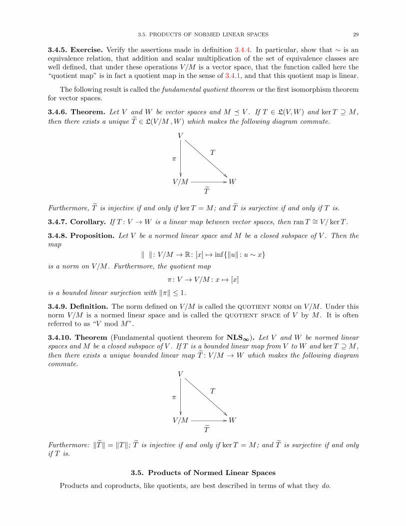
3.5. PRODUCTS OF NORMED LINEAR SPACES 29
3.4.5. Exercise. Verify the assertions made in definition 3.4.4. In particular, show that ∼ is anequivalence relation, that addition and scalar multiplication of the set of equivalence classes arewell defined, that under these operations V/M is a vector space, that the function called here the“quotient map” is in fact a quotient map in the sense of 3.4.1, and that this quotient map is linear.
The following result is called the fundamental quotient theorem or the first isomorphism theoremfor vector spaces.
3.4.6. Theorem. Let V and W be vector spaces and M V . If T ∈ L(V,W ) and kerT ⊇ M ,
then there exists a unique T ∈ L(V/M ,W ) which makes the following diagram commute.
V
π
T
!!V/M
T
// W
Furthermore, T is injective if and only if kerT = M ; and T is surjective if and only if T is.
3.4.7. Corollary. If T : V →W is a linear map between vector spaces, then ranT ∼= V/ kerT .
3.4.8. Proposition. Let V be a normed linear space and M be a closed subspace of V . Then themap
‖ ‖ : V/M → R : [x] 7→ inf‖u‖ : u ∼ xis a norm on V/M . Furthermore, the quotient map
π : V → V/M : x 7→ [x]
is a bounded linear surjection with ‖π‖ ≤ 1.
3.4.9. Definition. The norm defined on V/M is called the quotient norm on V/M . Under thisnorm V/M is a normed linear space and is called the quotient space of V by M . It is oftenreferred to as “V mod M”.
3.4.10. Theorem (Fundamental quotient theorem for NLS∞). Let V and W be normed linearspaces and M be a closed subspace of V . If T is a bounded linear map from V to W and kerT ⊇M ,
then there exists a unique bounded linear map T : V/M → W which makes the following diagramcommute.
V
π
T
!!V/M
T
// W
Furthermore: ‖T‖ = ‖T‖; T is injective if and only if kerT = M ; and T is surjective if and onlyif T is.
3.5. Products of Normed Linear Spaces
Products and coproducts, like quotients, are best described in terms of what they do.
30 3. NORMED LINEAR SPACES
3.5.1. Definition. Let A1 and A2 be objects in a category C. We say that the triple (P, π1, π2),where P is an object and πk : P → Ak (k = 1, 2) are morphisms, is a product of A1 and A2 if forevery object B and every pair of morphisms fk : B → Ak (k = 1, 2) there exists a unique morphismf : B → P such that fk = πk f for k = 1, 2.
It is conventional to say, “Let P be a product of . . . ” for, “Let (P, π1, π2) be a product of . . . ”.The product of A1 and A2 is often written as A1 ×A2 or as
∏k=1,2Ak.
In a particular category products may or may not exist. It is an interesting and elementary factthat whenever they exist they are unique (up to isomorphism), so that we may unambiguously speakof the product of two objects. When we say that a categorical object satisfying some condition(s) isunique up to isomorphism we mean, of course, that any two objects satisfying the condition(s) mustbe isomorphic. We will often use the phrase “essentially unique” for “unique up to isomorphism.”
3.5.2. Proposition. In any category products (if they exist) are essentially unique.
3.5.3. Example. In the category SET the product of two sets A1 and A2 exists and is in fact theusual Cartesian product A1 × A2 together with the usual coordinate projections πk : A1 × A2 →Ak : (a1, a2) 7→ ak.
3.5.4. Example. If V1 and V2 are vector spaces we make the Cartesian product V1 × V2 into avector space as follows. Define addition by
(u, v) + (w, x) := (u+ w, v + x)
and scalar multiplication byα(u, v) := (αu, αv) .
This makes V1 × V2 into a vector space and that this space together with the usual coordinateprojections πk : V1 × V2 → Vk : (v1, v2) 7→ vk (k = 1, 2) is a product in the category VEC. It isusually called the direct sum of V and W and is denoted by V ⊕W .
It often possible and desirable to take the product of an arbitrary family of objects in a category.Following is a generalization of definition 3.5.1.
3.5.5. Definition. Let(Aλ)λ∈Λ
be an indexed family of objects in a category C. We say that the
object P together with an indexed family(πλ)λ∈Λ
of morphisms πλ : P → Aλ is a product of the
objects Aλ if for every object B and every indexed family(fλ)λ∈Λ
of morphisms fλ : B → Aλ thereexists a unique map g : B → P such that fλ = πλ g for every λ ∈ Λ.
A category in which arbitrary products exist is said to be product complete. Many of thecategories we encounter in these notes are product complete.
3.5.6. Definition. Let(Sλ)λ∈Λ
be an indexed family of sets. The Cartesian product of the
indexed family, denoted by∏λ∈Λ Sλ or just
∏Sλ, is the set of all functions f : Λ→
⋃Sλ such that
f(λ) ∈ Sλ for each λ ∈ Λ. The maps πλ :∏Sλ → Sλ : f 7→ f(λ) are the canonical coordinate
projections. In many cases the notation fλ is more convenient than f(λ). (See, for example,example 3.5.8 below.)
3.5.7. Example. A very important special case of the preceding definition occurs when all of thesets Sλ are identical: say Sλ = A for every λ ∈ Λ. In this case the Cartesian product comprisesall the functions which map Λ into A. That is,
∏λ∈Λ Sλ = AΛ. Notice also that in this case the
coordinate projections are evaluation maps. For each λ the coordinate projection πλ takes eachpoint f in the product (that is, each function f from Λ into A) to f(λ) its value at λ. Briefly, eachcoordinate projection is an evaluation map at some point.
3.5.8. Example. What is Rn? It is just the set of all n-tuples of real numbers. That is, it is theset of functions from Nn = 1, 2, . . . , n into R. In other words Rn is just shorthand for RNn . InRn one usually writes xj for the jth coordinate of a vector x rather than x(j).
3.5. PRODUCTS OF NORMED LINEAR SPACES 31
3.5.9. Example. In the category SET the product of an indexed family of sets exists and is infact the Cartesian product of these sets together with the canonical coordinate projections.
3.5.10. Example. If(Vλ)λ∈Λ
is an indexed family of vector spaces we make the Cartesian product∏Vλ into a vector space as follows. Define addition and scalar multiplication pointwise: for f ,
g ∈∏Aλ and α ∈ R
(f + g)(λ) := f(λ) + g(λ)
and(αf)(λ) := αf(λ) .
This makes∏Vλ into a vector space, which is sometimes called the direct product of the spaces
Vλ, and this space together with the canonical coordinate projections (which are certainly linearmaps) is a product in the category VEC.
3.5.11. Example. Let V and W be normed linear spaces. On the Cartesian product V ×W define
‖(x, y)‖2 =√‖x‖2 + ‖y‖2,
‖(x, y)‖1 = ‖x‖+ ‖y‖,
and
‖(x, y)‖u = max‖x‖, ‖y‖ .The first of these is the Euclidean norm (or 2-norm) on V ×W , the second is the 1-norm, andthe last is the uniform norm. Verifying that these are all norms on V ×W is quite similar tothe arguments required in examples 3.1.1, 3.1.2, and 3.1.3. That they are equivalent norms is aconsequence of the following inequalities and proposition 3.1.37.
‖x‖+ ‖y‖ ≤√
2√‖x‖2 + ‖y‖2 ≤ 2 max‖x‖, ‖y‖ ≤ 2(‖x‖+ ‖y‖)
3.5.12. Convention. In the preceding example we defined three (equivalent) norms on the productspace V ×W . We will take the first of these ‖ ‖1 as the product norm on V ×W . Thus wheneverV and W are normed linear spaces, unless the contrary is specified we will regard the product V ×Was a normed linear space under this norm. Usually we write just ‖(x, y)‖ instead of ‖(x, y)‖1. Theproduct of the normed linear spaces V and W is usually denoted by V ⊕W and is called the directsum of V and W . (In the special case where V = W = R, what metric does the product norminduce on R2?)
3.5.13. Example. Show that product V ⊕W of normed linear spaces is in fact a product in thecategory NLS∞ of normed linear spaces and bounded linear maps.
3.5.14. Proposition. Let((xn, yn)
)be a sequence in the direct sum V ⊕W of two normed linear
spaces. Prove that((xn, yn)
)converges to a point (a, b) in V ⊕W if and only if xn → a in V and
yn → b in W .
3.5.15. Proposition. Addition is a continuous operation on a normed linear space V . That is,the map
A : V ⊕ V → V : (x, y) 7→ x+ y
is continuous.
3.5.16. Exercise. Give a very short proof (no ε’s or δ’s or open sets) that if (xn) and (yn) aresequences in a normed linear space which converge to a and b, respectively, then xn + yn → a+ b.
3.5.17. Proposition. Scalar multiplication is a continuous operation on a normed linear space Vin the sense that the map
S : K× V → V : (α, x) 7→ αx
is continuous.
32 3. NORMED LINEAR SPACES
3.5.18. Proposition. If B and C are subsets of a normed linear space and α is a scalar, then
(a) αB = αB; and(b) B + C ⊆ B + C.
3.5.19. Example. If B and C are closed subsets of a normed linear space, then it does notnecessarily follow that B + C is closed (and therefore B + C and B + C need not be equal).
3.5.20. Proposition. Let C1 and C2 be compact subsets of a normed linear space V . Then
(a) C1 × C2 is a compact subset of V × V , and(b) C1 + C2 is a compact subset of V .
3.5.21. Example. Let X be a topological space. Then the family C(X) of all continuous complexvalued functions on X is a vector space under the usual pointwise operations of addition and scalarmultiplication.
3.5.22. Example. Let X be a topological space. We denote by Cb(X) the family of all boundedcontinuous complex valued functions on X. It is a normed linear space under the uniform norm.In fact, it is a subspace of B(X) (see example 3.1.7).
3.5.23. Example. If S is a set and a ∈ S, then the evaluation functional
Ea : B(S)→ R : f 7→ f(a)
is a bounded linear functional on the space B(S) of all bounded real valued functions on S. If Shappens to be a topological space then we may also regard Ea as a member of the dual space ofCb(S). (In either case, what is ‖Ea‖?)
3.5.24. Definition. Let A be an algebra on which a norm has been defined. Suppose that addi-tionally the submultiplicative property
‖xy‖ ≤ ‖x‖ ‖y‖
is satisfied for all x, y ∈ A. Then A is a normed algebra. We make one further requirement: ifthe algebra A is unital, then
‖1‖ = 1 .
In this case A is a unital normed algebra.
3.5.25. Example. In example 3.1.7 we showed that the family B(S) of bounded real valuedfunctions on a set S is a normed linear space under the uniform norm. It is also a commutativeunital normed algebra.
3.5.26. Proposition. Multiplication is a continuous operation on a normed algebra V in the sensethat the map
M : V × V → V : (x, y) 7→ xy
is continuous.
Hint for proof . If you can prove that multiplication on the real numbers is continuous you canalmost certainly prove that it is continuous on arbitrary normed algebras.
3.5.27. Example. The family Cb(X) of bounded continuous real valued functions on a topologicalspace X is, under the usual pointwise operations and the uniform norm, a commutative unitalnormed algebra. (See example 3.5.22.)
3.5.28. Example. The family B(V ) of all (bounded linear) operators on a normed linear space Vis a unital normed algebra. (See 3.2.9 and 3.2.10.)
3.6. COPRODUCTS OF NORMED LINEAR SPACES 33
3.6. Coproducts of Normed Linear Spaces
Coproducts are like products—except all the arrows are reversed.
3.6.1. Definition. Let A1 and A2 be objects in a category C. The triple (Q, ι1, ι2), (Q is an objectand ιk : Ak → Q, k = 1, 2 are morphisms) is a coproduct of A1 and A2 if for every object B andevery pair of morphisms fk : Ak → B (k = 1,2) there exists a unique morphism f : P → B suchthat fk = f ιk for k = 1, 2.
3.6.2. Proposition. In any category coproducts (if they exist) are essentially unique.
3.6.3. Definition. Let A and B be sets. When A and B are disjoint we will often use the notationA ] B instead of A ∪ B (to emphasize the disjointness of A and B). When C = A ] B we saythat C is the disjoint union of A and B. Similarly we frequently choose to write the union of apairwise disjoint family A of sets as
⊎A. And the notation
⊎λ∈ΛAλ may be used to denote the
union of a pairwise disjoint indexed family Aλ : λ ∈ Λ of sets. When C =⊎A or C =
⊎λ∈ΛAλ
we say that C is the disjoint union of the appropriate family.
3.6.4. Definition. In the preceding definition we introduced the notation A ]B for the union oftwo disjoint sets A and B. We now extend this notation somewhat and allow ourselves to takethe disjoint union of sets A and B even if they are not disjoint. We “make them disjoint” byidentifying (in the obvious way) the set A with the set A′ = (a, 1) : a ∈ A and B with the setB′ = (b, 2) : b ∈ B. Then we denote the union of A′ and B′, which are disjoint, by A ] B andcall it the disjoint union of A and B.
In general, if(Aλ)λ∈Λ
is an indexed family of sets, its disjoint union,⊎λ∈Λ
Aλ is defined to be⋃(Aλ, λ) : λ ∈ Λ.
3.6.5. Example. In the category SET the coproduct of two sets A1 and A2 exists and is theirdisjoint union A1 ]A2 together with the obvious inclusion maps ιk : Ak → A1 ]A2 (k = 1, 2).
It is interesting to observe that while the product and coproduct of a finite collection of objectsin the category SET are quite different, in the more complex category VEC they turn out to beexactly the same thing.
3.6.6. Example. If V1 and V2 are vector spaces make the Cartesian product V1× V2 into a vectorspace as in example 3.5.4. This space together with the obvious injections is a coproduct in thecategory VEC.
It often possible and desirable to take the coproduct of an arbitrary family of objects in acategory. Following is a generalization of definition 3.6.1.
3.6.7. Definition. Let(Aλ)λ∈Λ
be an indexed family of objects in a category C. We say that the
object C together with an indexed family(ιλ)λ∈Λ
of morphisms ιλ : Aλ → C is a coproduct of
the objects Aλ if for every object B and every indexed family(fλ)λ∈Λ
of morphisms fλ : Aλ → Bthere exists a unique map g : C → B such that fλ = g ιλ for every λ ∈ Λ. The usual notation forthe coproduct of the objects Aλ is
∐λ∈ΛAλ.
3.6.8. Example. In the category SET the coproduct of an indexed family of sets exists and isthe disjoint union of these sets.
3.6.9. Definition. Let S be a set and V be a vector space. The support of a function f : S → Vis s ∈ S : f(s) 6= 0.
3.6.10. Example. If(Vλ)λ∈Λ
is an indexed family of vector spaces we make the Cartesian product
into a vector space as in example 3.5.10. The set of functions f belonging to∏Vλ which have finite
support (that is, which are nonzero only finitely often) is clearly a subspace of∏Vλ. This subspace
is the direct sum of the spaces Vλ. It is denoted by⊕
λ∈Λ Vλ. This space together with theobvious injective maps (which are linear) is a coproduct in the category VEC.
34 3. NORMED LINEAR SPACES
3.6.11. Exercise. What are the coproducts in the category NLS∞ ?
3.6.12. Exercise. Identify the product and coproduct of two spaces V and W in the categoryNLS1 of normed linear spaces and linear contractions.
3.7. Nets
Nets (sometimes called generalized sequences) are useful for characterizing many properties ofgeneral topological spaces. In such spaces they are used in basically the same way as sequences areused in metric spaces.
3.7.1. Definition. A preordered set in which every pair of elements has an upper bound is adirected set.
3.7.2. Example. If S is a set, then FinS is a directed set under inclusion ⊆.
3.7.3. Definition. Let S be a set and Λ be a directed set. A mapping x : Λ→ S is a net in S (ora net of members of S). The value of x at λ ∈ Λ is usually written x
λ(rather than x(λ)) and the
net x itself is often denoted by(xλ
)λ∈Λ
or just(xλ
).
3.7.4. Example. The most obvious examples of nets are sequences. These are functions whosedomain is the (preordered) set N of natural numbers.
3.7.5. Definition. A net x =(xλ
)is said to eventually have some specified property if there
exists λ0 ∈ Λ such that xλ
has that property whenever λ ≥ λ0; and it has the property frequentlyif for every λ0 ∈ Λ there exists λ ∈ Λ such that λ ≥ λ0 and x
λhas the property.
3.7.6. Definition. A neighborhood of a point in a topological space is any set which containsan open set containing the point.
3.7.7. Definition. A net x in a topological space X converges to a point a ∈ X if it is eventuallyin every neighborhood of a. In this case a is the limit of x and we write
xλ λ∈Λ
// a
or just xλ→ a. When limits are unique we may also use the notation limλ∈Λ xλ = a or, more
simply, limxλ
= a.The point a in X is a cluster point of the net x if x is frequently in every neighborhood of a.
3.7.8. Definition. Let (X,T) be a topological space. A subfamily S ⊆ T is a subbase for thetopology T if the family of all finite intersections of members of S is a base for T.
3.7.9. Example. Let X be a topological space and a ∈ X. A base for the family of neighborhoodsof the point a is a family Ba of neighborhoods of a with the property that every neighborhood ofa contains at least one member of Ba. In general, there are many choices for a neighborhood baseat a point. Once such a base is chosen we refer to its members as basic neighborhoods of a.
Let Ba be a base for the family of neighborhoods at a. Order Ba by containment (the reverseof inclusion); that is, for U , V ∈ Ba set
U V if and only if U ⊇ V .This makes Ba into a directed set. Now (using the axiom of choice) choose one element xU fromeach set U ∈ Ba. Then (x
U) is a net in X and x
U→ a.
The next two propositions assure us that in order for a net to converge to a point a in atopological space it is sufficient that it be eventually in every basic (or even subbasic) neighborhoodof a.
3.7.10. Proposition. Let B be a base for the topology on a topological space X and a be a pointof X. A net (xλ) converges to a if and only if it is eventually in every neighborhood of a whichbelongs to B.
3.7. NETS 35
3.7.11. Proposition. Let S be a subbase for the topology on a topological space X and a be apoint of X. A net (xλ) converges to a if and only if it is eventually in every neighborhood of awhich belongs to S.
3.7.12. Example. Let J = [a, b] be a fixed interval in the real line, x = (x0, x1, . . . , xn) be an(n+1)-tuple of points of J , and t = (t1, . . . , tn) be an n-tuple. The pair (x; t) is a partition withselection of the interval J if:
(a) xk−1 < xk for 1 ≤ k ≤ n;(b) tk ∈ [xk−1, xk] for 1 ≤ k ≤ n;(c) x0 = a; and(d) xn = b.
The idea is that x partitions the interval into subintervals and tk is the point selected from the kth
subinterval. If x = (x0, x1, . . . , xn), then x denotes the set x0, x1, . . . , xn. Let P = (x; s) andQ = (y; t) be partitions (with selections) of the interval J . We write P 4 Q and say that Q is arefinement of P if x ⊆ y. Under the relation 4 the family P of partitions with selection onJ is a directed (but not partially ordered) set.
Now suppose f is a bounded function on the interval J and P = (x; t) is a partition of J inton subintervals. Let ∆xk := xk − xk−1 for 1 ≤ k ≤ n. Then define
Sf (P ) :=n∑k=1
f(tk) ∆xk .
Each such sum Sf (P ) is a Riemann sum of f on J . Notice that since P is a directed set, Sfis a net of real numbers. If the net Sf of Riemann sums converges we say that the function f isRiemann integrable. The limit of the net Sf (when it exists) is the Riemann integral of f
over the interval J and is denoted by∫ ba f(x) dx.
3.7.13. Example. In a topological space X with the indiscrete topology (where the only open setsare X and the empty set) every net in the space converges to every point of the space.
3.7.14. Example. In a topological space X with the discrete topology (where every subset of Xis open) a net in the space converges if and only if it is eventually constant.
3.7.15. Definition. A Hausdorff topological space is one in which every pair of distinct pointscan be separated by open sets; that is, for every pair x and y of distinct points in the space thereexist open neighborhoods of x and y that are disjoint.
As example 3.7.13 shows nets in general topological spaces need not have unique limits. Aspace does not require very restrictive assumptions however to make this pathology go away. Forlimits to be unique it is sufficient to require that a space be Hausdorff. Interestingly, it turns outthat this condition is also necessary.
3.7.16. Proposition. If X is a topological space, then the following are equivalent:
(a) X is Hausdorff.(b) No net in X can converge to more than one point.(c) The diagonal in X ×X is closed.
(The diagonal of a set S is (s, s) : s ∈ S ⊆ S × S.)
3.7.17. Example. Recall from beginning calculus that the nth partial sum of an infinite series∑∞k=1 xk is defined to be sn =
∑nk=1 xk. The series is said to converge if the sequence (sn) of
partial sums converges and, if the series converges, its sum is the limit of the sequence (sn) ofpartial sums. Thus, for example, the infinite series
∑∞k=1 2−k converges and its sum is 1.
The idea of summing an infinite series depends heavily on the fact that the partial sums ofthe series are linearly ordered by inclusion. The “partial sums” of a net of numbers need not be
36 3. NORMED LINEAR SPACES
partially ordered, so we need a new notion of “summation”, sometimes referred to as unorderedsummation.
3.7.18. Notation. If A is a set we denote by FinA the family of all finite subsets of A. (Notethat this is a directed set under the relation ⊆.)
3.7.19. Definition. Let A ⊆ R. For every F ∈ FinA define SF to be the sum of the numbersin F , that is, SF =
∑F . Then S =
(SF)F∈FinA
is a net in R. If this net converges, the set A of
numbers is said to be summable; the limit of the net is the sum of A and is denoted by∑A.
3.7.20. Definition. A net (xλ) of real numbers is increasing if λ ≤ µ implies xλ ≤ xµ. A net ofreal (or complex) numbers is bounded if its range is.
3.7.21. Example. Let f(n) = 2−n for every n ∈ N, and let x : Fin(N) → R be defined byx(A) =
∑n∈A f(n).
(a) The net x is increasing.(b) The net x is bounded.(c) The net x converges to 1.(d) The set of numbers 1
2 ,14 ,
18 ,
116 , . . . is summable and its sum is 1.
3.7.22. Example. In a metric space every convergent sequence is bounded. Give an example toshow that a convergent net in a metric space (even in R) need not be bounded.
It is familiar from beginning calculus that bounded increasing sequences in R converge. Thepreceding example is a special case of a more general observation: bounded increasing nets in Rconverge.
3.7.23. Proposition. Every bounded increasing net(xλ
)λ∈Λ
of real numbers converges and
limxλ
= supxλ
: λ ∈ Λ .
3.7.24. Example. Let (xk) be a sequence of distinct positive real numbers and A = xk : k ∈ N.Then
∑A (as defined above) is equal to the sum of the series
∑∞k=1 xk.
3.7.25. Example. The set
1k : k ∈ N
is not summable and the infinite series
∑∞k=1
1k does not
converge.
3.7.26. Example. The set
(−1)k 1k : k ∈ N
is not summable but the infinite series
∑∞k=1(−1)k 1
kdoes converge.
3.7.27. Proposition. Every summable subset of real numbers is countable.
Hint for proof. If A is a summable set of real numbers and n ∈ N, how many members of Acan be larger than 1/n?
In proposition 3.7.16 we have already seen one example of a way in which nets characterize atopological property: a space is Hausdorff if and only if limits of nets in the space are unique (whenthey exist). Here is another topological property—continuity at a point—that can be convenientlycharacterized in terms of nets.
3.7.28. Proposition. Let X and Y be topological spaces. A function f : X → Y is continuous ata point a in X if and only if f
(xλ
)→ f(a) in Y whenever
(xλ
)is a net converging to a in X.
In metric spaces we characterize closures and interiors of sets in terms of sequences. For generaltopological spaces we must replace sequences by nets.
In defining the terms “interior” and “closure” we have choices similar to the ones we had indefining “convex hull” in 3.1.25. There is an ’abstract’ definition and there is a ‘constructive’ one.You may find it helpful to recall proposition 3.1.26 and the paragraph preceding it.
3.8. THE HAHN-BANACH THEOREMS 37
3.7.29. Definition. The interior of a set A in a topological space X is the largest open subsetof X contained in A; that is, the union of all open subsets of X contained in A. The interior of Ais denoted by A.
3.7.30. Proposition. The preceding definition makes sense. Furthermore, a point a in a topologicalspace X is in the interior of a subset A of X if and only if every net in X that converges to a iseventually in A.
Hint for proof . One direction is easy. In the other use proposition 3.7.10 and the sort of netconstructed in example 3.7.9.
3.7.31. Definition. The closure of a set A in a topological space X is the smallest closed subsetof X containing A; that is, the intersection of all closed subsets of X which contain A. The closureof A is denoted by A.
3.7.32. Proposition. The preceding definition makes sense. Furthermore, a point b in a topologicalspace X belongs to the closure of a subset A of X if and only if some net in A converges to b.
3.7.33. Corollary. A subset A of a topological space is closed if and only if the limit of everyconvergent net in A belongs to A.
3.8. The Hahn-Banach Theorems
It should be said at the beginning that referring to “the” Hahn-Banach theorem is somethingof a misnomer. A writer who claims to be using the Hahn-Banach theorem may be using any of adozen or so versions of the theorem or its corollaries. What do the various versions have in common?Basically they assure us that normed linear spaces have, in general, a rich enough supply of boundedlinear functionals to make their dual spaces useful tools in studying the spaces themselves. Thatis, they guarantee an interesting and productive duality theory. Below we consider four versions ofthe ‘theorem’ and three of its corollaries. We will succumb to usual practice: when in the sequelwe make use of any of these results, we will say we are using ‘the’ Hahn-Banach theorem.
As is often the case in mathematics the attribution of these results to Hahn and Banach is a bitpeculiar. It seems that the basic insights were due originally to Eduard Helly. For an interestinghistory of the ‘Hahn-Banach’ results see [29].
Incidentally, in the name “Banach”, the “a”’s are pronounced as in car and the “ch” as inchaos; and the accent is on the first syllable (BAH-nakh).
3.8.1. Definition. A real valued function f on a real vector space V is a sublinear functionalif f(x+ y) ≤ f(x) + f(y) and f(αx) = αf(x) for all x, y ∈ V and α ≥ 0.
3.8.2. Example. A norm on a real vector space is a sublinear functional.
Our first version of the Hahn-Banach theorem is pure linear algebra and applies only to realvector spaces. It allows us to extend certain linear functionals on such spaces from subspaces tothe whole space.
3.8.3. Theorem (Hahn-Banach theorem I). Let M be a subspace of a real vector space V and pbe a sublinear functional on V . If f is a linear functional on M such that f ≤ p on M , then f hasan extension g to all of V such that g ≤ p on V .
Hint for proof . In this theorem the notation h ≤ p means that domh ⊆ dom p = V and thath(x) ≤ p(x) for all x ∈ domh. In this case we say that h is dominated by p. We write f 4 g if gis an extension of f (that is, if f(x) = g(x) for all x ∈ dom f).
Let S be the family of all real valued linear functionals on subspaces of V which are extensionsof f and are dominated by p. The family S is partially ordered by 4. Use Zorn’s lemma to producea maximal element g of S. The proof is finished if you can show that dom g = V .
38 3. NORMED LINEAR SPACES
To this end, suppose to the contrary that there is a vector c ∈ V which does not belongto D = dom g. Prove first that
g(y)− p(y − c) ≤ −g(x) + p(x+ c) (3.8.1)
for all x, y ∈ D. Conclude that there is a number γ which lies between the supremum of all thenumbers on the left side of (3.8.1) and the infimum of those on the right.
Let E be the span of D ∪ c. Define h on E by h(x+ αc) = g(x) + αγ for x ∈ D and α ∈ R.Now show h ∈ S. (Take α > 0 and work separately with h(x+ αc) and h(x− αc).)
The next theorem is the version of theorem 3.8.3 for spaces with complex scalars. It is sometimesreferred to as the Bohnenblust-Sobczyk-Suhomlinov theorem.
3.8.4. Theorem (Hahn-Banach theorem II). Let V be a complex vector space, p be a seminormon V , and M be a subspace of V . If f : M → C is a linear functional such that |f | ≤ p, then f hasan extension g which is a linear functional on all of V satisfying |g| ≤ p.
Hint for proof . This result is essentially a straightforward corollary to the real version of theHahn-Banach theorem given above in 3.8.3. Let VR be the real vector space associated with V(same vectors but using only R as the scalar field). Notice that if u is the real part of f (thatis, u(x) = <(f(x)) for each x ∈ M), then u is an R-linear functional on M (that is, f(x + y) =f(x) + f(y) and f(αx) = αf(x) for all x, y ∈ M and all α ∈ R) and f(x) = u(x) − i u(ix). Andconversely, if u is a R-linear functional on some vector space, then f(x) := u(x) − i u(ix) definesa (complex valued) linear functional on that space. Notice also that if u is the real part of f ,then |u(x)| ≤ p for all x if and only if |f(x)| ≤ p for all x. With these observations in mind justapply 3.8.3 to the real part of f on VR.
Next is perhaps the most often used version of the Hahn-Banach theorem.
3.8.5. Theorem (Hahn-Banach theorem III). Let M be a vector subspace of a (real or complex)normed linear space V . Then every continuous linear functional f on M has an extension g to allof V such that ‖g‖ = ‖f‖.
Hint for proof . Consider the function p : V → R : x 7→ ‖f‖‖x‖.
It is sometimes useful, when proving a theorem, to consider the possibility of more “natural”or even more “obvious” proofs. On occasion one is rewarded by an enlightening simplification andclarification of complex material. And sometimes one is fooled.
3.8.6. Exercise. Your buddy Fred R. Dimm thinks he has discovered a really simple direct proof ofthe version of the Hahn-Banach theorem given in proposition 3.8.5: A continuous linear functionalf defined on a (linear) subspace M of a normed linear space V can be extended to a continuouslinear functional g on all of V without increasing its norm. He says that all one needs to do is letN be any vector space complement of M and let B be a (Hamel) basis for N . Define g(e) = 0 forevery vector e ∈ B and g = f on M . Then extend g by linearity to all of V . Surely, Fred says, g islinear by construction and its norm has not increased since we have made it zero where it was notpreviously defined. Show Fred the error of his ways.
3.8.7. Theorem (Hahn-Banach theorem IV). Let V be a (real or complex) normed linear space,M be a vector subspace of V , and suppose that y ∈ V is such that d := dist(y,M) > 0. Then thereexists a functional g ∈ V ∗ such that g→(M) = 0, g(y) = d, and ‖g‖ = 1.
Hint for proof . Let N := span (M ∪ y) and define f : N → K : x+αy 7→ αd (x ∈M , α ∈ K).
The most useful special case of the preceding theorem is when M = 0 and y 6= 0. This tellsus that the only way for f(x) to vanish for every f ∈ V ∗ is for x to be the zero vector.
3.8.8. Corollary. Let V be a normed linear space and x ∈ V . If f(x) = 0 for every f ∈ V ∗, thenx = 0.
3.8. THE HAHN-BANACH THEOREMS 39
3.8.9. Definition. A family G(S) of scalar valued functions on a set S separates points of S iffor every pair x and y of distinct points in S there exists a function f ∈ G(S) such that f(x) 6= f(y).
3.8.10. Corollary. If V is a normed linear space, then V ∗ separates points of V .
3.8.11. Corollary. Let V be a normed linear space and x ∈ V . Then there exists f ∈ V ∗ suchthat ‖f‖ = 1 and f(x) = ‖x‖.
3.8.12. Proposition. Let V be a normed linear space, x1, . . . , xn be a linearly independent subsetof V , and α1, . . . , αn be scalars. Then there exists an f in V ∗ such that f(xk) = αk for 1 ≤ k ≤ n.
Hint for proof . For x =∑n
k=1 βkxk let g(x) =∑n
k=1 αkβk.
3.8.13. Proposition. Let V be a normed linear space and 0 6= x ∈ V . Then
‖x‖ = max|f(x)| : f ∈ V ∗ and ‖f‖ ≤ 1 .
The use of max instead of sup in the preceding proposition is intentional. The propositionclaims that there exists an f in the closed unit ball of V ∗ such that f(x) = ‖x‖.
3.8.14. Definition. A subset A of a topological space X is dense in X if A = X. The space Xis separable if it contains a countable dense subset.
3.8.15. Example. The space Kn is separable under its usual topology; that is the topology itinherits from its usual norm. (See 3.1.1, 1.2.17, and 3.1.34.)
3.8.16. Example. Given the discrete topology the real line R is not separable.
3.8.17. Proposition. Let V be a normed linear space. If V ∗ is separable, then so is V .

CHAPTER 4
HILBERT SPACES
For the most elementary facts about Hilbert spaces I can think of no better introduction thanthe first two chapters of Halmos’s classic text [23]. Another good introduction is [55]. You mayalso find chapters 3 and 9 of [33] and chapter 4 of [22] helpful. For a start towards more seriousexplorations into the mysteries of Hilbert space look at [8], [9], and [25].
4.1. Definition and Examples
A Hilbert space is a complete inner product space. In more detail:
4.1.1. Definition. In proposition 1.2.15 we showed how an inner product on a vector space inducesa norm on the space and in proposition 1.2.17 how a norm in turn induces a metric. If an innerproduct space is complete with respect to this metric it is a Hilbert space. Similarly, a Banachspace is a complete normed linear space and a Banach algebra is a complete normed algebra.
4.1.2. Example. Under the inner product defined in example 1.2.4 Kn is a Hilbert space.
4.1.3. Example. Under the inner products in example 1.2.5 l2 = l2(N) and l2(Z) are Hilbertspaces.
4.1.4. Example. Under the inner product defined in example 1.2.6 C([a, b]) is not a Hilbert space.
4.1.5. Example. Let C(X) = C(X,C) be the family of all continuous complex valued functions ona compact Hausdorff space X. Under the uniform norm
‖f‖u := sup|f(x)| : 0 ≤ x ≤ 1C(X) is a Banach space. If the space X is not compact we can make the set Cb(X) of all boundedcontinuous complex valued functions on X into a Banach space in the same way. When the scalarfield is R we will write C(X,R) for the family of continuous real valued functions on X. It too is aBanach space.
4.1.6. Example. The inner product space lc of all sequences (an) of complex numbers which areeventually zero (see example 1.2.34) is not a Hilbert space.
4.1.7. Example. Let µ be a positive measure on a σ-algebra A of subsets of a set S. If you areunacquainted with general measure theory, a casual introduction to Lebesgue measure on the realline should suffice for examples which appear in these notes. A complex valued function f on Sis measurable if the inverse image under f of every Borel set (equivalently, every open set) inC belongs to A. We define an equivalence relation ∼ on the family of measurable complex valuedfunctions by setting f ∼ g whenever f and g differ on a set of measure zero, that is, wheneverµ(x ∈ S : f(x) 6= g(x)) = 0. We adopt conventional notation and denote the equivalence classcontaining f by f itself (rather than something more logical such as [f ]). We denote the familyof (equivalence classes of) measurable complex valued functions on S by M(S, µ). A functionf ∈M(S, µ) is square integrable if
∫S |f(x)|2 dµ(x) <∞. We denote the family of (equivalence
classes of) square integrable functions on S by L2(S, µ). For every f , g ∈ L2(S, µ) define
〈f, g〉 :=
∫Sf(x)g(x) dµ(x) .
With this inner product (and the obvious pointwise vector space operations) L2(S, µ) is a Hilbertspace.
41
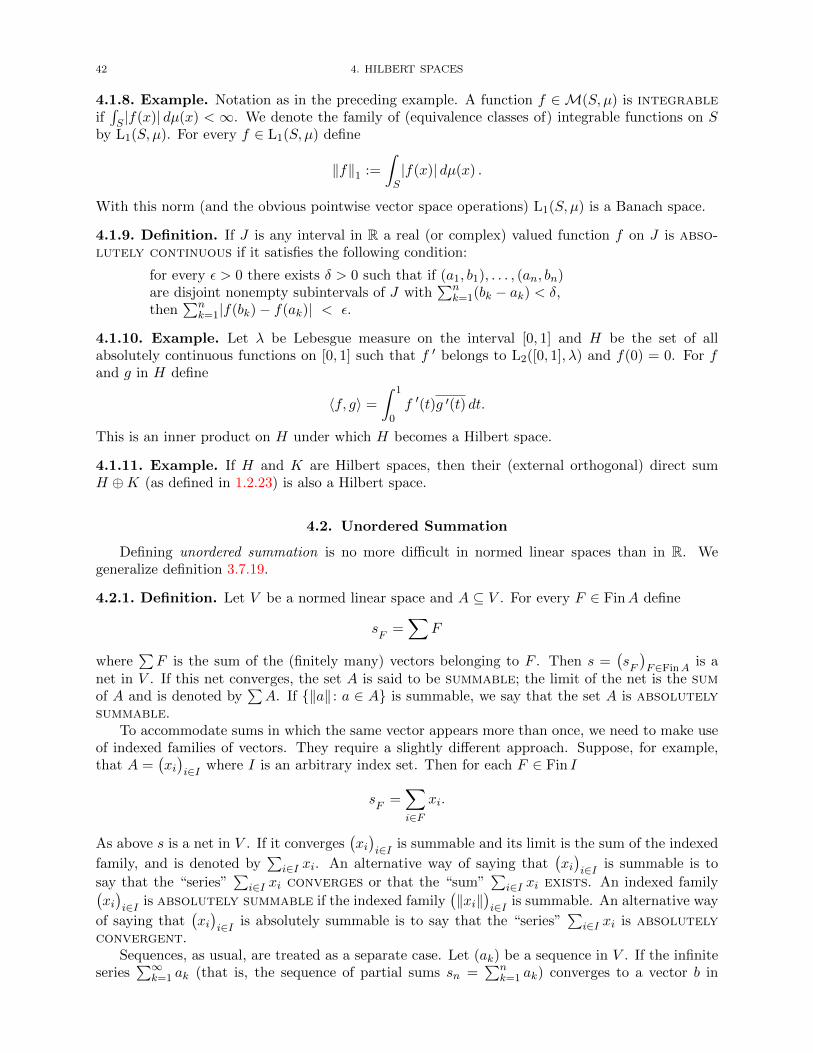
42 4. HILBERT SPACES
4.1.8. Example. Notation as in the preceding example. A function f ∈ M(S, µ) is integrableif∫S |f(x)| dµ(x) < ∞. We denote the family of (equivalence classes of) integrable functions on S
by L1(S, µ). For every f ∈ L1(S, µ) define
‖f‖1 :=
∫S|f(x)| dµ(x) .
With this norm (and the obvious pointwise vector space operations) L1(S, µ) is a Banach space.
4.1.9. Definition. If J is any interval in R a real (or complex) valued function f on J is abso-lutely continuous if it satisfies the following condition:
for every ε > 0 there exists δ > 0 such that if (a1, b1), . . . , (an, bn)are disjoint nonempty subintervals of J with
∑nk=1(bk − ak) < δ,
then∑n
k=1|f(bk)− f(ak)| < ε.
4.1.10. Example. Let λ be Lebesgue measure on the interval [0, 1] and H be the set of allabsolutely continuous functions on [0, 1] such that f ′ belongs to L2([0, 1], λ) and f(0) = 0. For fand g in H define
〈f, g〉 =
∫ 1
0f ′(t)g ′(t) dt.
This is an inner product on H under which H becomes a Hilbert space.
4.1.11. Example. If H and K are Hilbert spaces, then their (external orthogonal) direct sumH ⊕K (as defined in 1.2.23) is also a Hilbert space.
4.2. Unordered Summation
Defining unordered summation is no more difficult in normed linear spaces than in R. Wegeneralize definition 3.7.19.
4.2.1. Definition. Let V be a normed linear space and A ⊆ V . For every F ∈ FinA define
sF
=∑
F
where∑F is the sum of the (finitely many) vectors belonging to F . Then s =
(sF
)F∈FinA
is anet in V . If this net converges, the set A is said to be summable; the limit of the net is the sumof A and is denoted by
∑A. If ‖a‖ : a ∈ A is summable, we say that the set A is absolutely
summable.To accommodate sums in which the same vector appears more than once, we need to make use
of indexed families of vectors. They require a slightly different approach. Suppose, for example,that A =
(xi)i∈I where I is an arbitrary index set. Then for each F ∈ Fin I
sF
=∑i∈F
xi.
As above s is a net in V . If it converges(xi)i∈I is summable and its limit is the sum of the indexed
family, and is denoted by∑
i∈I xi. An alternative way of saying that(xi)i∈I is summable is to
say that the “series”∑
i∈I xi converges or that the “sum”∑
i∈I xi exists. An indexed family(xi)i∈I is absolutely summable if the indexed family
(‖xi‖
)i∈I is summable. An alternative way
of saying that(xi)i∈I is absolutely summable is to say that the “series”
∑i∈I xi is absolutely
convergent.Sequences, as usual, are treated as a separate case. Let (ak) be a sequence in V . If the infinite
series∑∞
k=1 ak (that is, the sequence of partial sums sn =∑n
k=1 ak) converges to a vector b in
4.2. UNORDERED SUMMATION 43
V , then we say that the sequence (ak) is summable or, equivalently, that the series∑∞
k=1 ak is aconvergent series. The vector b is called the sum of the series
∑∞k=1 ak and we write
∞∑k=1
ak = b .
It is clear that a necessary and sufficient condition for a series∑∞
k=1 ak to be convergent or,equivalently, for the sequence (ak) to be summable, is that there exist a vector b in V such that∥∥∥∥b− n∑
k=1
ak
∥∥∥∥→ 0 as n→∞. (4.2.1)
4.2.2. Proposition. A normed linear space V is complete if and only if every absolutely summablesequence in V is summable.
Hint for proof . Let (xn) be a Cauchy sequence in a normed linear space in which every abso-lutely summable sequence is summable. Find a subsequence
(xnk)
of (xn) such that ‖xn−xm‖ < 2−k
whenever m, n ≥ nk. If we let y1 = xn1 and yj = xnj − xnj−i for j > 1, then (yj) is absolutelysummable.
4.2.3. Proposition. If(xi)i∈I and
(yi)i∈I are summable indexed families in a normed linear space
and α is a scalar, then(αxi)i∈I and
(xi + yi
)i∈I are summable; and∑
i∈Iαxi = α
∑i∈I
xi
and ∑i∈I
xi +∑i∈I
yi =∑i∈I
(xi + yi).
4.2.4. Remark. One frequently finds some version of the following “proposition” in textbooks.
If∑
i∈I xi = u and∑
i∈I xi = v in a Hilbert (or Banach) space, then u = v.
(I once saw a 6 line proof of this.) Of which result is this a trivial consequence?
4.2.5. Proposition. If(xi)i∈I is a summable indexed family of vectors in a Hilbert space H and
y is a vector in H, then(〈xi, y〉
)i∈I is a summable indexed family of scalars and∑
i∈I〈xi, y〉 =
⟨∑i∈I
xi, y
⟩.
The following is a generalization of example 4.1.3.
4.2.6. Example. Let I be an arbitrary nonempty set and l2(I) be the set of all complex valuedfunctions x on I such that
∑i∈I |xi|2 <∞. For all x, y ∈ l2(I) define
〈x, y〉 =∑i∈I
x(i)y(i).
(a) If x ∈ l2(I), then x(i) = 0 for all but countably many i.(b) The map (x, y) 7→ 〈x, y〉 is an inner product on the vector space l2(I).(c) The space l2(I) is a Hilbert space.
4.2.7. Proposition. Let (xn) be a sequence in a Hilbert space. If the sequence regarded as anindexed family is summable, then the infinite series
∑∞k=1 xk converges.
4.2.8. Example. The converse of proposition 4.2.7 does not hold.
The direct sum of two Hilbert spaces is a Hilbert space.
44 4. HILBERT SPACES
4.2.9. Proposition. If H and K are Hilbert spaces, then their (orthogonal) direct sum (as definedin 1.2.23) is a Hilbert space.
We can also take the product of more than two Hilbert spaces—even an infinite family of them.
4.2.10. Proposition. Let(Hi
)i∈I be an indexed family of Hilbert spaces. A function x : I →
⋃Hi
belongs to H =⊕i∈I
Hi if x(i) ∈ Hi for every i and if∑
i∈I‖x(i)‖2 < ∞. Defining 〈 , 〉 on H by
〈x, y〉 :=∑
i∈I〈x(i), y(i)〉 makes H into an Hilbert space.
4.2.11. Definition. The Hilbert space defined in the preceding proposition is the (externalorthogonal) direct sum of the Hilbert spaces Hi.
4.2.12. Exercise. Is the direct sum defined above (with appropriate morphisms) a product in thecategory HSp of Hilbert spaces and bounded linear maps? Is it a coproduct?
4.3. Hilbert space Geometry
4.3.1. Convention. In the context of Hilbert spaces the word “subspace” will always mean closedvector subspace. The reason for this is that we want a subspace of a Hilbert space to be a Hilbertspace in its own right; that is to say, a subspace of a Hilbert space should be a subobject in thecategory of Hilbert spaces (and appropriate morphisms). To indicate that M is a subspace of H wewrite M 4 H. A (not necessarily closed) vector subspace of a Hilbert space is also called a linearsubspace or a linear manifold.
4.3.2. Definition. Let A be a nonempty subset of a Banach (or Hilbert) space B. We define theclosed linear span of A (denoted by
∨A) to be the smallest subspace of B containing A; that
is, the intersection of all subspaces of B which contain A.
As with definitions 3.1.25, 3.7.29, and 3.7.31, we need to show that the preceding one makessense.
4.3.3. Proposition. The preceding definition makes sense. Furthermore, a vector is in the closedlinear span of A if and only if it belongs to the closure of the linear span of A.
4.3.4. Theorem (Minimizing Vector Theorem). If C is a nonempty closed convex subset of aHilbert space H and a ∈ Cc, then there exists a unique b ∈ C such that ‖b− a‖ ≤ ‖x− a‖ for everyx ∈ C.
x
a
33
// b
C
Hint for proof . For the existence part let d = inf‖x − a‖ : x ∈ C. Choose a sequence (yn)of vectors in C such that ‖yn − a‖ → d. To prove that the sequence (yn) is Cauchy, apply theparallelogram law 1.2.26 to the vectors ym − a and yn − a for m, n ∈ N. The uniqueness part issimilar: apply the parallelogram law to the vectors b − a and c − a where b and c are two vectorssatisfying the conclusion of the theorem.
4.3. HILBERT SPACE GEOMETRY 45
4.3.5. Example. The vector space R2 under the uniform metric is a Banach space. To see thatin this space the minimizing vector theorem does not hold take C to be the closed unit ball aboutthe origin and a to be the point (2, 0).
4.3.6. Example. The sets
C1 =
f ∈ C([0, 1]) :
∫ 1/2
0f −
∫ 1
1/2f = 1
and C2 =
f ∈ L1([0, 1], λ) :
∫ 1
0f = 1
are examples that show that neither the existence nor the uniqueness claims of the minimizingvector theorem necessarily holds in a Banach space. (The symbol λ denotes Lebesgue measure.)
4.3.7. Theorem (Vector Decomposition Theorem). Let H be a Hilbert space and M be a (closedlinear) subspace of H. Then for every x ∈ H there exist unique vectors y ∈ M and z ∈ M⊥ suchthat x = y + z.
Hint for proof . Assume x /∈ M (otherwise the result is trivial). Explain how we know thatthere exists a unique vector y ∈M such that
‖x− y‖ ≤ ‖x−m‖ (4.3.1)
for all m ∈ M . Explain why it is enough, for the existence part of the proof, to prove that x − yis perpendicular to every unit vector m ∈ M . Explain why it is true that for every unit vectorm ∈M
‖x− y‖2 ≤ ‖x− (y + λm)‖2 (4.3.2)
where λ := 〈x− y,m〉.
4.3.8. Corollary. If M is a subspace of a Hilbert space H, then H = M ⊕M⊥.
4.3.9. Example. The preceding result says that every subspace of a Hilbert space is a directsummand. This result need not be true if M is assumed to be just a linear subspace of the space.For example, notice that M = lc (see example 4.1.6) is a linear subspace of the Hilbert space l2(see example 4.1.3) but M⊥ = 0.
4.3.10. Corollary. A vector subspace A of a Hilbert space H is dense in H if and only if A⊥ = 0.
4.3.11. Proposition. Every proper subspace of a Hilbert space has empty interior.
4.3.12. Proposition. If a Hamel basis for a Hilbert space is not finite, then it is uncountable.
Hint for proof . Suppose the space has a countably infinite basis e1, e2, e3, . . . . For each n ∈ Nlet Mn = spane1, e2, . . . , en. Apply the Baire category theorem (see [16], theorem 29.3.20) to⋃∞n=1Mn keeping in mind the preceding proposition.
4.3.13. Proposition. Let H be a Hilbert space. Then the following hold:
(a) if A ⊆ H, then A ⊆ A⊥⊥;(b) if A ⊆ B ⊆ H, then B⊥ ⊆ A⊥;(c) if M is a subspace of H, then M = M⊥⊥; and(d) if A ⊆ H, then
∨A = A⊥⊥.
4.3.14. Proposition. Let M and N be subspaces of a Hilbert space. Then
(a) (M +N)⊥ = (M ∪N)⊥ = M⊥ ∩N⊥, and(b) (M ∩N)⊥ = M⊥ +N⊥.
4.3.15. Proposition. Let V be a normed linear space. There exists an inner product on V whichinduces the norm on V if and only if the norm satisfies the parallelogram law 1.2.26.
46 4. HILBERT SPACES
Hint for proof . We say that an inner product 〈 · , · 〉 on V induces the norm ‖ · ‖ if ‖x‖ =√〈x, x〉 holds for every x in V .) To prove that if a norm satisfies the parallelogram law then it is
induced by an inner product, use the equation in the polarization identity 1.2.28 as a definition.Prove first that 〈y, x〉 = 〈x, y〉 for all x, y ∈ V and that 〈x, x〉 > 0 whenever x 6= 0. Next, forarbitrary z ∈ V , define a function f : V → C : x 7→ 〈x, z〉. Prove that
f(x+ y) + f(x− y) = 2f(x) (∗)
for all x, y ∈ V . Use this to prove that f(αx) = αf(x) for all x ∈ V and α ∈ R. (Start with αbeing a natural number.) Then show that f is additive. (If u and v are arbitrary elements of V letx = u + v and y = u − v. Use (∗).) Finally prove that f(αx) = αf(x) for complex α by showingthat f(ix) = i f(x) for all x ∈ V .
4.4. Orthonormal Sets and Bases
4.4.1. Definition. A nonempty subset E of a Hilbert space is orthonormal if e ⊥ f for everypair of distinct vectors e and f in E and ‖e‖ = 1 for every e ∈ E.
4.4.2. Proposition. In an inner product space every orthonormal set is linearly independent.
4.4.3. Proposition (Bessel’s inequality). Let H be a Hilbert space and E be an orthonormal subsetof H. For every x ∈ H ∑
e∈E‖〈x, e〉‖2 ≤ ‖x‖2 .
4.4.4. Corollary. If E is an orthonormal subset of a Hilbert space H and x ∈ H, then e ∈E : 〈x, e〉 6= 0 is countable.
4.4.5. Proposition. Let E be an orthonormal set in a Hilbert space H. Then the following areequivalent.
(a) E is a maximal orthonormal set.(b) If x ⊥ E, then x = 0 (E is total).(c)
∨E = H (E is a complete orthonormal set).
(d) x =∑e∈E〈x, e〉e for all x ∈ H. (Fourier expansion)
(e) 〈x, y〉 =∑e∈E〈x, e〉〈e, y〉 for all x, y ∈ H. (Parseval’s identity.)
(f) ‖x‖2 =∑e∈E|〈x, e〉|2 for all x ∈ H. (Parseval’s identity.)
4.4.6. Definition. If H is a Hilbert space, then an orthonormal set E satisfying any one (henceall) of the conditions in proposition 4.4.5 is called an orthonormal basis for H (or a completeorthonormal set in H, or a Hilbert space basis for H). Notice that this is a very differentthing from the usual (Hamel) basis for a vector space (see 1.1.10). For a Hilbert space the basisvectors are required to be of length one and to be mutually perpendicular (conditions which makeno sense in a vector space); but it is not necessary that every vector in the space be a linearcombination of the basis vectors.
4.4.7. Proposition. If E is an orthonormal subset of a Hilbert space H, then there exists anorthonormal basis for H which contains E.
4.4.8. Corollary. Every nonzero Hilbert space has a basis.
4.4.9. Proposition. If E is an orthonormal subset of a Hilbert space H and x ∈ H, then 〈x, e〉e :e ∈ E is summable.
4.4. ORTHONORMAL SETS AND BASES 47
4.4.10. Example. For each n ∈ N let en be the sequence in l2 whose nth coordinate is 1 and allthe other coordinates are 0. Then en : n ∈ N is an orthonormal basis for l2. This is the usual(or standard) orthonormal basis for l2.
4.4.11. Exercise. A function f : R→ C of the form
f(t) = a0 +
n∑k=1
(ak cos kt+ bk sin kt)
where a0, . . . , an, b1, . . . , bn are complex numbers is a trigonometric polynomial.
(a) Explain why complex valued 2π-periodic functions on the real line R are often identifiedwith complex valued functions on the unit circle T.
(b) Some authors say that a trigonometric polynomial is a function of the form
f(t) =n∑
k=−ncke
ikt
where c1, . . . , cn are complex numbers. Explain carefully why this is exactly the same asthe preceding definition.
(c) Justify the use of the term trigonometric polynomial.(d) Prove that every continuous 2π-periodic function on R is the uniform limit of a sequence
of trigonometric polynomials.
4.4.12. Proposition. Let E be a basis for a Hilbert space H and x ∈ H. If x =∑
e∈E αee, thenαe = 〈x, e〉 for each e ∈ E.
4.4.13. Proposition. Consider the Hilbert space L2([0, 2π],C) of (equivalence classes of complexvalued, square integrable functions on [0, 2π] with inner product
〈f, g〉 =1
2π
∫ 2π
0f(x)g(x) dx.
For every integer n (positive, negative, or zero) let en(x) = einx for all x ∈ [0, 2π]. Then the set ofthese functions en for n ∈ Z is an orthonormal basis for L2([0, 2π],C).
4.4.14. Example. The sum of the infinite series∞∑k=1
1
k2isπ2
6.
Hint for proof . Let f(x) = x for 0 ≤ x ≤ 2π. Regard f as a member of L2([0, 2π]). Find ‖f‖in two ways.
The next proposition allows us to define the notion of the dimension of a Hilbert space. (Infinite dimensional spaces it agrees with the vector space concept.)
4.4.15. Proposition. Any two orthonormal bases of a Hilbert space have the same cardinality(that is, they are in one-to-one correspondence).
Proof. See [23], page 29, Theorem 1.
4.4.16. Definition. The dimension of a Hilbert space is the cardinality of any orthonormal basisfor the space.
4.4.17. Proposition. A Hilbert space is separable if and only if it has a countable orthonormalbasis.
Proof. See [33], page 171, Theorem 3.6-4.
48 4. HILBERT SPACES
4.5. The Riesz-Frechet Theorem
4.5.1. Example. Let H be a Hilbert space and a ∈ H. Define ψa : H → C : x 7→ 〈x, a〉. Thenψa ∈ H∗.
Now we generalize theorem 1.2.38 to the infinite dimensional setting. This result is sometimescalled the Riesz representation theorem (which invites confusion with the more substantial resultabout representing certain linear functionals as measures) or the little Riesz representation theorem.This theorem says that the only continuous linear functionals on a Hilbert space are the functionsψa defined in 4.5.1. In other words, given a continuous linear functional f on a Hilbert space thereis a unique vector a in the space such that the action of f on a vector x can be represented simplyby taking the inner product of x with a.
4.5.2. Theorem (Riesz-Frechet Theorem). If f ∈ H∗ where H is a Hilbert space, then there existsa unique vector a in H such that f = ψa. Furthermore, ‖a‖ = ‖ψa‖.
Hint for proof . For the case f 6= 0, choose a unit vector z in (ker f)⊥. Notice that for every
x ∈ H the vector x− f(x)f(z) z belongs to ker f .
4.5.3. Corollary. The kernel of every nonzero bounded linear functional on a Hilbert space hascodimension 1.
Hint for proof . The codimension of a subspace of a Hilbert space is the dimension of itsorthogonal complement. This is really a corollary to the proof of the Riesz-Frechet theorem. Inour proof we found that the vector representing the bounded linear functional f was a (nonzero)multiple of a unit vector in (ker f)⊥. What would happen if there were two linearly independentvectors in (ker f)⊥?
4.5.4. Definition. Recall that a mapping T : V → W between complex vector spaces is conju-gate linear if T (x + y) = Tx + Ty and T (αx) = αTx for all x, y ∈ V and α ∈ C. A bijectiveconjugate linear map is an anti-isomorphism.
4.5.5. Example. For a Hilbert space H, the mapping ψ : H → H∗ : a 7→ ψa defined in exam-ple 4.5.1 is an isometric anti-isomorphism between H and its dual space.
4.5.6. Definition. A conjugate linear mapping C : V → V from a vector space into itself whichsatisfies C2 = idV is called a conjugation on V .
4.5.7. Example. Complex conjugation z 7→ z is an example of a conjugation in the vector space C.
4.5.8. Example. Let H be a Hilbert space and E be a basis for H. Then the map x 7→∑
e∈E〈e, x〉eis a conjugation and an isometry on H.
The term “anti-isomorphism” is a bit misleading. It suggests something entirely different froman isomorphism. In fact, an anti-isomorphism is nearly as good as an isomorphism. The nextproposition says in essence that a Hilbert space and its dual are isomorphic because they are anti-isomorphic.
4.5.9. Proposition. Let H be a Hilbert space, ψ : H → H∗ be the anti-isomorphism defined in 4.5.1(see 4.5.5), and C be the conjugation defined in 4.5.8. Then the composite Cψ−1 is an isometricisomorphism from H∗ onto H.
4.5.10. Corollary. Every Hilbert space is isometrically isomorphic to its dual.
4.5.11. Proposition. Let H be a Hilbert space and ψ : H → H∗ be the anti-isomorphism definedin 4.5.1 (see 4.5.5). If we define 〈f, g〉 := 〈ψ−1g, ψ−1f〉 for all f , g ∈ H∗, then H∗ becomes aHilbert space isometrically isomorphic to H. The resulting norm on H∗ is its usual norm.
4.5.12. Corollary. Every Hilbert space is reflexive.
4.6. STRONG AND WEAK TOPOLOGIES ON HILBERT SPACES 49
4.5.13. Example. Let H be the collection of all absolutely continuous complex valued functionsf on [0, 1] such that f(0) = 0 and f ′ ∈ L2([0, 1], λ). Define an inner product on H by
〈f, g〉 :=
∫ 1
0f ′(t) g′(t) dt.
We already know that H is a Hilbert space (see example 4.1.10) Fix t ∈ (0, 1]. Define
Et : H → C : f 7→ f(t).
Then Et is a bounded linear functional on H. What is its ‖Et‖? What vector g in H representsthe functional Et?
4.5.14. Exercise. One afternoon your pal Fred R. Dimm comes to you with a problem. “Look,”he says, “On L2 = L2(R,R) the evaluation functional E0, which evaluates each member of L2 at 0,is clearly a bounded linear functional. So by the Riesz representation theorem there should be somefunction g in L2 such that f(0) = 〈f, g〉 =
∫∞−∞ fg for all f in L2. But that’s a property of the
‘δ-function’, which I was told doesn’t exist. What am I doing wrong?” Give Freddy some (helpful)advice.
4.5.15. Exercise. Later the same afternoon Freddy’s back. After considering the advice you gavehim (in the preceding problem) he has revised his question by letting the domain of E0 be the setof bounded continuous real valued functions defined on R. Patiently you explain to Freddy thatthere are now at least two things wrong his invocation of the ‘δ-function’. What are they?
4.5.16. Exercise. The nightmare continues. It’s 11 P. M. and Freddy’s back again. This time(happily having given up on δ-functions) he wants to apply the representation theorem to thefunctional “evaluation at zero” on the space l2(Z). Can he do it? Explain.
4.6. Strong and Weak Topologies on Hilbert Spaces
We recall briefly the definition and crucial facts about weak topologies. For a more detailedintroduction to this class of topologies see any good textbook on topology or section 11.4 of mynotes [16].
4.6.1. Definition. Suppose that S is a set, that for every α ∈ A (where A is an arbitrary indexset) Xα is a topological space, and that fα : S → Xα for every α ∈ A. Let
S = fα←(Uα) : Uα⊆ Xα and α ∈ A .
Use the family S as a subbase for a topology on S. This topology is called the weak topologyinduced by (or determined by) the functions fα.
4.6.2. Proposition. Under the weak topology (defined above) on a set S each of the functions fαis continuous; in fact the weak topology is the weakest topology on S under which these functionsare continuous.
4.6.3. Proposition. Let X be a topological space with the weak topology determined by a familyF of functions. Prove that a function g : W → X, where W is a topological space, is continuous ifand only if f g is continuous for every f ∈ F .
4.6.4. Definition. Let(Aλ)λ∈Λ
be an indexed family of topological spaces. The weak topology on
the Cartesian product∏Aλ induced by the family of coordinate projections πλ (see definition 3.5.6)
is called the product topology.
4.6.5. Proposition. The product of a family of Hausdorff spaces is Hausdorff.
4.6.6. Example. Let Y be a topological space with the weak topology (see definition 4.6.1) de-termined by an indexed family (fα)α∈A of functions where for each α ∈ A the codomain of fαis a topological space Xα. Then a net
(yλ
)λ∈Λ
in Y converges to a point a ∈ Y if and only if
fα(yλ)
λ∈Λ// fα(a) for every α ∈ A.
50 4. HILBERT SPACES
4.6.7. Example. If Y =∏α∈AXα is a product of nonempty topological spaces with the product
topology (see definition 4.6.4), then a net(yλ
)in Y converges to a ∈ Y if and only if
(yλ
)α→ aα
for every α ∈ A.
4.6.8. Example. If V and W are normed linear spaces, then the product topology on V ×W isthe same as the topology induced by the product norm on V ⊕W .
The next example illustrates the inadequacy of sequences when dealing with general topologicalspaces.
4.6.9. Example. Let F = F([0, 1]) be the set of all functions f : [0, 1]→ R and give F the producttopology, that is, the weak topology determined by the evaluation functionals
Ex : F → [0, 1] : f 7→ f(x)
where x ∈ [0, 1]. Thus a basic open neighborhood of a point g ∈ F is determined by a finite set ofpoints A ∈ Fin[0.1] and a number ε > 0:
U(g ; A ; ε) := f ∈ F : |f(t)− g(t)| < ε for all t ∈ A.
(What is usual name for this topology?) Let G be the set of all functions in F having finite support.Then
(a) the constant function 1 belongs to G,(b) there is a net of functions in G which converges to 1, but(c) no sequence in G converges to 1.
4.6.10. Definition. A net (xλ) in a Hilbert space H is said to converge weakly to a point a
in H if 〈xλ, y〉 // 〈a, y〉 for every y ∈ H. In this case we write xλ
w // a. In a Hilbert space anet is said to converge strongly (or converge in norm) if it converges with respect to thetopology induced by the norm. This is the usual type of convergence in a Hilbert space. If we
wish to emphasize a distinction between modes of convergence we may write xλ
s // a for strongconvergence.
4.6.11. Exercise. Explain why the topology on a Hilbert space generated by the weak convergenceof nets is in fact a weak topology in the usual topological sense of the term.
When we say that a subset of a Hilbert space H is weakly closed we mean that it is closedwith respect to the weak topology on H; a set is weakly compact if it is compact in the weaktopology on H; and so on. A function f : H → H is weakly continuous if it is continuous as amap from H with the weak topology into H with the weak topology.
4.6.12. Exercise. Let H be a Hilbert space and (xλ) be a net in H.
(a) If xλ
s // a in H, then xλ
w // a in H(b) The strong (norm) topology on H is stronger (bigger) than the weak topology.(c) Show by example that the converse of (a) does not hold.(d) Is the norm on H weakly continuous?
(e) If xλ
w // a in H and if ‖xλ‖ // ‖a‖, then x
λ
s // a in H.(f) If a linear map T : H → H is (strongly) continuous, then it is weakly continuous.
4.6.13. Exercise. Let H be an infinite dimensional Hilbert space. Consider the following subsetsof H:
(a) the open unit ball;(b) the closed unit ball;(c) the unit sphere;(d) a closed linear subspace.
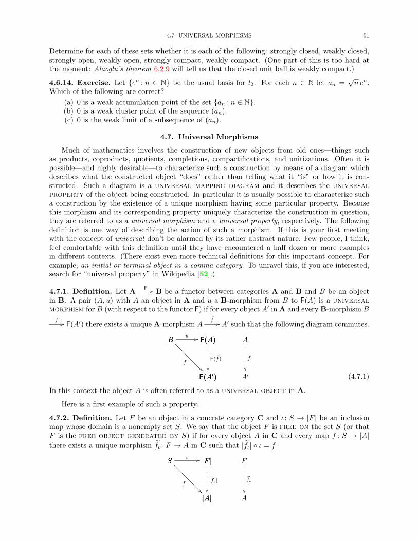
4.7. UNIVERSAL MORPHISMS 51
Determine for each of these sets whether it is each of the following: strongly closed, weakly closed,strongly open, weakly open, strongly compact, weakly compact. (One part of this is too hard atthe moment: Alaoglu’s theorem 6.2.9 will tell us that the closed unit ball is weakly compact.)
4.6.14. Exercise. Let en : n ∈ N be the usual basis for l2. For each n ∈ N let an =√n en.
Which of the following are correct?
(a) 0 is a weak accumulation point of the set an : n ∈ N.(b) 0 is a weak cluster point of the sequence (an).(c) 0 is the weak limit of a subsequence of (an).
4.7. Universal Morphisms
Much of mathematics involves the construction of new objects from old ones—things suchas products, coproducts, quotients, completions, compactifications, and unitizations. Often it ispossible—and highly desirable—to characterize such a construction by means of a diagram whichdescribes what the constructed object “does” rather than telling what it “is” or how it is con-structed. Such a diagram is a universal mapping diagram and it describes the universalproperty of the object being constructed. In particular it is usually possible to characterize sucha construction by the existence of a unique morphism having some particular property. Becausethis morphism and its corresponding property uniquely characterize the construction in question,they are referred to as a universal morphism and a universal property, respectively. The followingdefinition is one way of describing the action of such a morphism. If this is your first meetingwith the concept of universal don’t be alarmed by its rather abstract nature. Few people, I think,feel comfortable with this definition until they have encountered a half dozen or more examplesin different contexts. (There exist even more technical definitions for this important concept. Forexample, an initial or terminal object in a comma category. To unravel this, if you are interested,search for “universal property” in Wikipedia [52].)
4.7.1. Definition. Let AF // B be a functor between categories A and B and B be an object
in B. A pair (A, u) with A an object in A and u a B-morphism from B to F(A) is a universalmorphism for B (with respect to the functor F) if for every object A′ in A and every B-morphism B
f // F(A′) there exists a unique A-morphism Af // A′ such that the following diagram commutes.
B F(A)u //B
F(A′)
f
F(A)
F(A′)
F(f)
A
A′
f
(4.7.1)
In this context the object A is often referred to as a universal object in A.
Here is a first example of such a property.
4.7.2. Definition. Let F be an object in a concrete category C and ι : S → |F | be an inclusionmap whose domain is a nonempty set S. We say that the object F is free on the set S (or thatF is the free object generated by S) if for every object A in C and every map f : S → |A|there exists a unique morphism fι : F → A in C such that |fι| ι = f .
S |F |ι //S
|A|
f
|F |
|A|
|fι|
F
A
fι
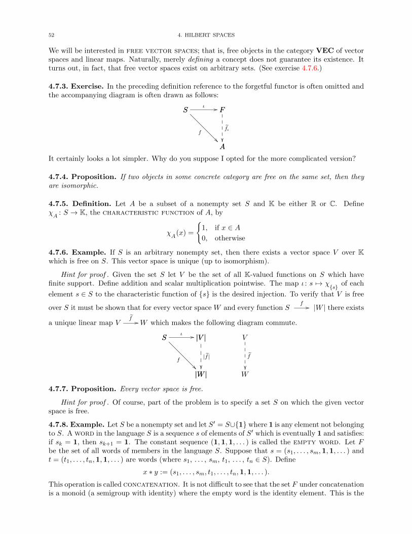
52 4. HILBERT SPACES
We will be interested in free vector spaces; that is, free objects in the category VEC of vectorspaces and linear maps. Naturally, merely defining a concept does not guarantee its existence. Itturns out, in fact, that free vector spaces exist on arbitrary sets. (See exercise 4.7.6.)
4.7.3. Exercise. In the preceding definition reference to the forgetful functor is often omitted andthe accompanying diagram is often drawn as follows:
S Fι //S
A
f
F
A
fι
It certainly looks a lot simpler. Why do you suppose I opted for the more complicated version?
4.7.4. Proposition. If two objects in some concrete category are free on the same set, then theyare isomorphic.
4.7.5. Definition. Let A be a subset of a nonempty set S and K be either R or C. DefineχA
: S → K, the characteristic function of A, by
χA
(x) =
1, if x ∈ A0, otherwise
4.7.6. Example. If S is an arbitrary nonempty set, then there exists a vector space V over Kwhich is free on S. This vector space is unique (up to isomorphism).
Hint for proof . Given the set S let V be the set of all K-valued functions on S which havefinite support. Define addition and scalar multiplication pointwise. The map ι : s 7→ χs of each
element s ∈ S to the characteristic function of s is the desired injection. To verify that V is free
over S it must be shown that for every vector space W and every function Sf // |W | there exists
a unique linear map Vf //W which makes the following diagram commute.
S |V |ι //S
|W |
f
|V |
|W |
|f |
V
W
f
4.7.7. Proposition. Every vector space is free.
Hint for proof . Of course, part of the problem is to specify a set S on which the given vectorspace is free.
4.7.8. Example. Let S be a nonempty set and let S′ = S∪1 where 1 is any element not belongingto S. A word in the language S is a sequence s of elements of S′ which is eventually 1 and satisfies:if sk = 1, then sk+1 = 1. The constant sequence (1,1,1, . . . ) is called the empty word. Let Fbe the set of all words of members in the language S. Suppose that s = (s1, . . . , sm,1,1, . . . ) andt = (t1, . . . , tn,1,1, . . . ) are words (where s1, . . . , sm, t1, . . . , tn ∈ S). Define
x ∗ y := (s1, . . . , sm, t1, . . . , tn,1,1, . . . ).
This operation is called concatenation. It is not difficult to see that the set F under concatenationis a monoid (a semigroup with identity) where the empty word is the identity element. This is the
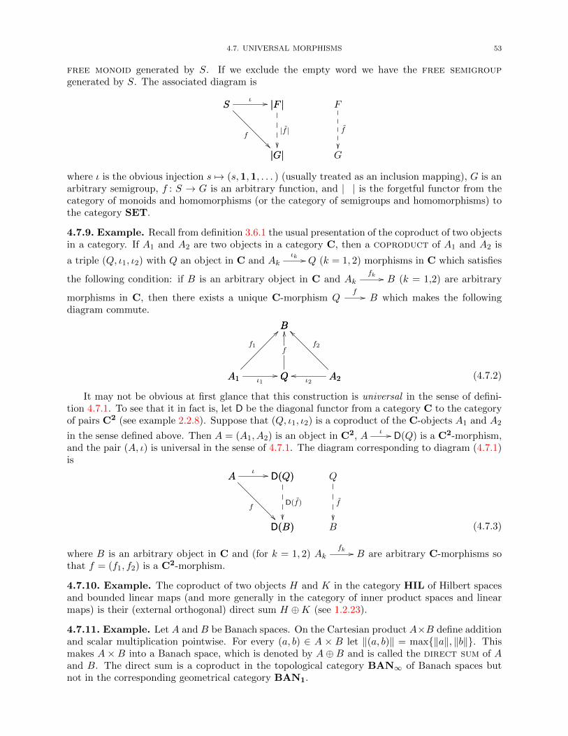
4.7. UNIVERSAL MORPHISMS 53
free monoid generated by S. If we exclude the empty word we have the free semigroupgenerated by S. The associated diagram is
S |F |ι //S
|G|
f
|F |
|G|
|f |
F
G
f
where ι is the obvious injection s 7→ (s,1,1, . . . ) (usually treated as an inclusion mapping), G is anarbitrary semigroup, f : S → G is an arbitrary function, and | | is the forgetful functor from thecategory of monoids and homomorphisms (or the category of semigroups and homomorphisms) tothe category SET.
4.7.9. Example. Recall from definition 3.6.1 the usual presentation of the coproduct of two objectsin a category. If A1 and A2 are two objects in a category C, then a coproduct of A1 and A2 is
a triple (Q, ι1, ι2) with Q an object in C and Akιk // Q (k = 1, 2) morphisms in C which satisfies
the following condition: if B is an arbitrary object in C and Akfk // B (k = 1,2) are arbitrary
morphisms in C, then there exists a unique C-morphism Qf // B which makes the following
diagram commute.
A1 Qι1// Q A2oo
ι2
B
A1
??
f1
B
Q
OO
f
B
A2
__
f2
(4.7.2)
It may not be obvious at first glance that this construction is universal in the sense of defini-tion 4.7.1. To see that it in fact is, let D be the diagonal functor from a category C to the categoryof pairs C2 (see example 2.2.8). Suppose that (Q, ι1, ι2) is a coproduct of the C-objects A1 and A2
in the sense defined above. Then A = (A1, A2) is an object in C2, Aι // D(Q) is a C2-morphism,
and the pair (A, ι) is universal in the sense of 4.7.1. The diagram corresponding to diagram (4.7.1)is
A D(Q)ι //A
D(B)
f
D(Q)
D(B)
D(f)
Q
B
f
(4.7.3)
where B is an arbitrary object in C and (for k = 1, 2) Akfk // B are arbitrary C-morphisms so
that f = (f1, f2) is a C2-morphism.
4.7.10. Example. The coproduct of two objects H and K in the category HIL of Hilbert spacesand bounded linear maps (and more generally in the category of inner product spaces and linearmaps) is their (external orthogonal) direct sum H ⊕K (see 1.2.23).
4.7.11. Example. Let A and B be Banach spaces. On the Cartesian product A×B define additionand scalar multiplication pointwise. For every (a, b) ∈ A × B let ‖(a, b)‖ = max‖a‖, ‖b‖. Thismakes A×B into a Banach space, which is denoted by A⊕B and is called the direct sum of Aand B. The direct sum is a coproduct in the topological category BAN∞ of Banach spaces butnot in the corresponding geometrical category BAN1.
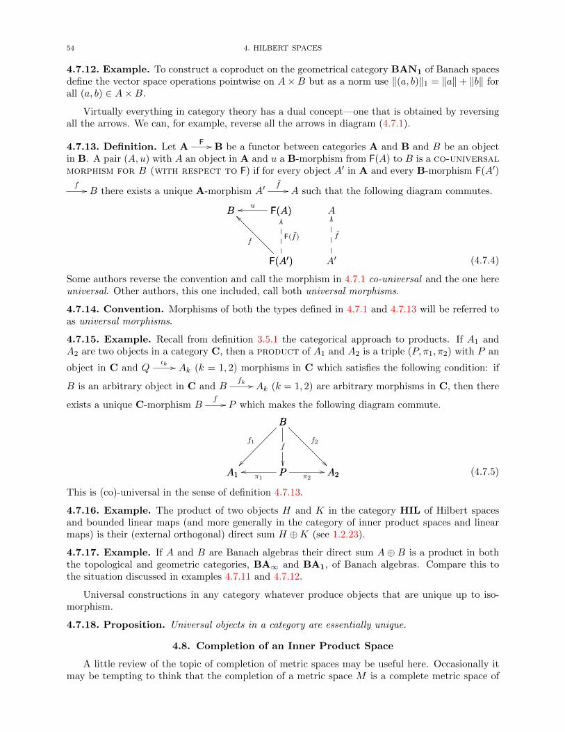
54 4. HILBERT SPACES
4.7.12. Example. To construct a coproduct on the geometrical category BAN1 of Banach spacesdefine the vector space operations pointwise on A×B but as a norm use ‖(a, b)‖1 = ‖a‖+ ‖b‖ forall (a, b) ∈ A×B.
Virtually everything in category theory has a dual concept—one that is obtained by reversingall the arrows. We can, for example, reverse all the arrows in diagram (4.7.1).
4.7.13. Definition. Let AF // B be a functor between categories A and B and B be an object
in B. A pair (A, u) with A an object in A and u a B-morphism from F(A) to B is a co-universalmorphism for B (with respect to F) if for every object A′ in A and every B-morphism F(A′)
f // B there exists a unique A-morphism A′f // A such that the following diagram commutes.
B F(A)oo uB
F(A′)
__
f
F(A)
F(A′)
OO
F(f)
A
A′
OO
f
(4.7.4)
Some authors reverse the convention and call the morphism in 4.7.1 co-universal and the one hereuniversal. Other authors, this one included, call both universal morphisms.
4.7.14. Convention. Morphisms of both the types defined in 4.7.1 and 4.7.13 will be referred toas universal morphisms.
4.7.15. Example. Recall from definition 3.5.1 the categorical approach to products. If A1 andA2 are two objects in a category C, then a product of A1 and A2 is a triple (P, π1, π2) with P an
object in C and Qιk // Ak (k = 1, 2) morphisms in C which satisfies the following condition: if
B is an arbitrary object in C and Bfk // Ak (k = 1, 2) are arbitrary morphisms in C, then there
exists a unique C-morphism Bf // P which makes the following diagram commute.
A1 Pooπ1
P A2π2//
B
A1
f1
B
P
f
B
A2
f2
(4.7.5)
This is (co)-universal in the sense of definition 4.7.13.
4.7.16. Example. The product of two objects H and K in the category HIL of Hilbert spacesand bounded linear maps (and more generally in the category of inner product spaces and linearmaps) is their (external orthogonal) direct sum H ⊕K (see 1.2.23).
4.7.17. Example. If A and B are Banach algebras their direct sum A ⊕ B is a product in boththe topological and geometric categories, BA∞ and BA1, of Banach algebras. Compare this tothe situation discussed in examples 4.7.11 and 4.7.12.
Universal constructions in any category whatever produce objects that are unique up to iso-morphism.
4.7.18. Proposition. Universal objects in a category are essentially unique.
4.8. Completion of an Inner Product Space
A little review of the topic of completion of metric spaces may be useful here. Occasionally itmay be tempting to think that the completion of a metric space M is a complete metric space of
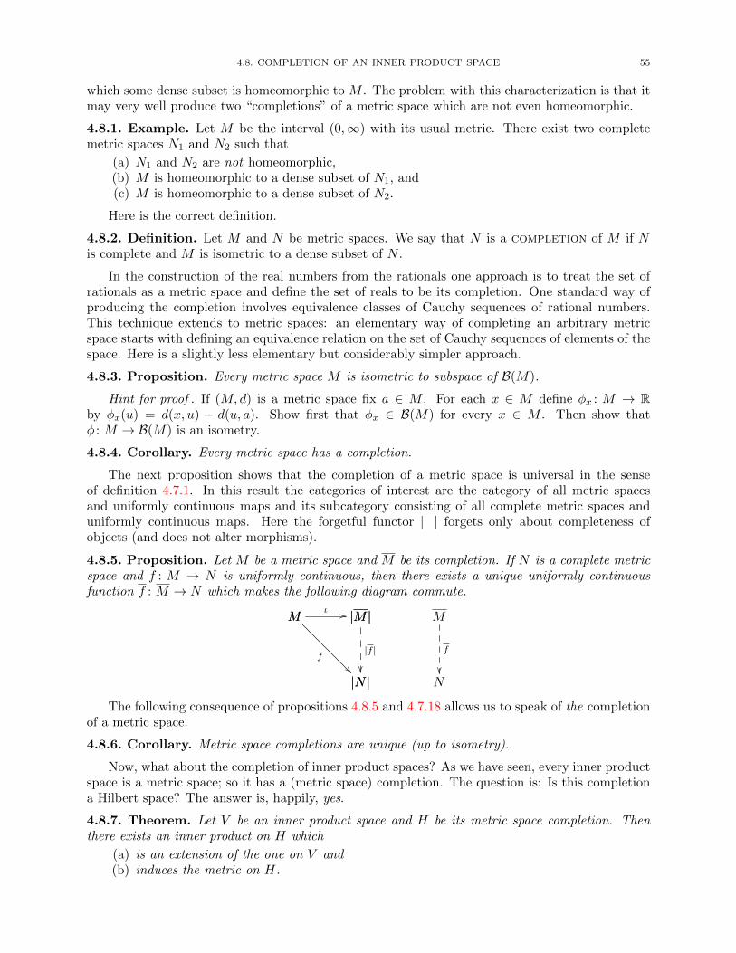
4.8. COMPLETION OF AN INNER PRODUCT SPACE 55
which some dense subset is homeomorphic to M . The problem with this characterization is that itmay very well produce two “completions” of a metric space which are not even homeomorphic.
4.8.1. Example. Let M be the interval (0,∞) with its usual metric. There exist two completemetric spaces N1 and N2 such that
(a) N1 and N2 are not homeomorphic,(b) M is homeomorphic to a dense subset of N1, and(c) M is homeomorphic to a dense subset of N2.
Here is the correct definition.
4.8.2. Definition. Let M and N be metric spaces. We say that N is a completion of M if Nis complete and M is isometric to a dense subset of N .
In the construction of the real numbers from the rationals one approach is to treat the set ofrationals as a metric space and define the set of reals to be its completion. One standard way ofproducing the completion involves equivalence classes of Cauchy sequences of rational numbers.This technique extends to metric spaces: an elementary way of completing an arbitrary metricspace starts with defining an equivalence relation on the set of Cauchy sequences of elements of thespace. Here is a slightly less elementary but considerably simpler approach.
4.8.3. Proposition. Every metric space M is isometric to subspace of B(M).
Hint for proof . If (M,d) is a metric space fix a ∈ M . For each x ∈ M define φx : M → Rby φx(u) = d(x, u) − d(u, a). Show first that φx ∈ B(M) for every x ∈ M . Then show thatφ : M → B(M) is an isometry.
4.8.4. Corollary. Every metric space has a completion.
The next proposition shows that the completion of a metric space is universal in the senseof definition 4.7.1. In this result the categories of interest are the category of all metric spacesand uniformly continuous maps and its subcategory consisting of all complete metric spaces anduniformly continuous maps. Here the forgetful functor | | forgets only about completeness ofobjects (and does not alter morphisms).
4.8.5. Proposition. Let M be a metric space and M be its completion. If N is a complete metricspace and f : M → N is uniformly continuous, then there exists a unique uniformly continuousfunction f : M → N which makes the following diagram commute.
M |M |ι //M
|N |
f
|M |
|N |
|f |
M
N
f
The following consequence of propositions 4.8.5 and 4.7.18 allows us to speak of the completionof a metric space.
4.8.6. Corollary. Metric space completions are unique (up to isometry).
Now, what about the completion of inner product spaces? As we have seen, every inner productspace is a metric space; so it has a (metric space) completion. The question is: Is this completiona Hilbert space? The answer is, happily, yes.
4.8.7. Theorem. Let V be an inner product space and H be its metric space completion. Thenthere exists an inner product on H which
(a) is an extension of the one on V and(b) induces the metric on H.

CHAPTER 5
HILBERT SPACE OPERATORS
5.1. Invertible Linear Maps and Isometries
5.1.1. Definition. A linear map T : H → K between two inner product spaces is inner productpreserving if 〈Tx, Ty〉 = 〈x, y〉 for all x, y ∈ H.
5.1.2. Proposition. Let T : H → K be a linear map between inner product spaces. Then thefollowing are equivalent:
(a) T is inner product preserving;(b) T is norm preserving; and(c) T is an isometry.
Just as was the case with normed linear spaces (see the very end of section 3.2) there are (atleast) two important categories in which the objects are Hilbert spaces:
(a) HSp = Hilbert spaces and bounded linear maps, and(b) HSp1 = Hilbert spaces and linear contractions.
In any category it is usual to define isomorphism to be an invertible morphism. Since it is the (topo-logical) category of Hilbert spaces and bounded linear maps that we encounter nearly exclusively inthese notes it might seem reasonable to apply the word “isomorphism” to the isomorphisms in thiscategory—in other words, to invertible maps; while an isomorphism in the more restrictive (geo-metric) category of Hilbert spaces and linear contractions might reasonably be called an isometricisomorphism. But this is not the convention. When most mathematicians think of a “Hilbert spaceisomorphism” they think of a map which preserves all the Hilbert space structure—including the in-ner product. Thus (invoking 5.1.2) the word “isomorphism” when applied to maps between Hilbertspaces has come, in most places, to mean isometric isomorphism. And consequently, the isomor-phisms in the more common category HSp are called invertible (bounded linear) maps. Recall also:We reserve the word “operator” for bounded linear maps from a space into itself.
5.1.3. Example. Define an operator T on the Hilbert space H = L2([0,∞)) by
Tf(t) =
f(t− 1), if t ≥ 1
0, if 0 ≤ t < 1.
Then T is an isometry but not an isometric isomorphism. If, on the other hand, H = L2(R) and Tmaps each f ∈ H to the function t 7→ f(t− 1), then T is an isometric isomorphism.
5.1.4. Example. Let H be the Hilbert space defined in example 4.1.10. Then the differentiationmapping D : f 7→ f ′ from H into L2([0, 1]) is an isometric isomorphism. What is its inverse?
5.1.5. Example. Let (Xi, µi) : i ∈ I be a family of σ-finite measure spaces. Make the disjoint
union X =⊎i∈I
Xi into a measure space (X,µ) in the usual way. Then L2(X,µ) is isometrically
isomorphic to the direct sum of the Hilbert spaces L2(Xi, µi).
5.1.6. Example. Let µ be Lebesgue measure on [−π2 ,
π2 ] and ν be Lebesgue measure on R. Let
(Uf)(x) =f(arctanx)√
1 + x2for all f ∈ L2(µ) and all x ∈ R. Then U is an isometric isomorphism
between L2([−π2 ,
π2 ], µ) and L2(R, ν).
57
58 5. HILBERT SPACE OPERATORS
5.1.7. Proposition. Every inner product preserving surjection from one Hilbert space to anotheris automatically linear.
5.1.8. Proposition. If T : H → K is a bounded linear map between Hilbert spaces, then
‖T‖ = sup|〈Tx, y〉| : ‖x‖ = ‖y‖ = 1 .
Hint for proof . Show first that ‖x‖ = sup|〈x, y〉| : ‖y‖ = 1.
5.1.9. Definition. A curve in a Hilbert space H is a continuous map from [0, 1] into H. A curveis simple if it is injective. If c is a curve and 0 ≤ a < b ≤ 1, then the chord of c corresponding tothe interval [a, b] is the vector c(b) − c(a). Two chords are non-overlapping if their associatedparameter intervals have at most an endpoint in common.
Halmos, in [24], illustrates the roominess of infinite dimensional Hilbert spaces by means of thefollowing elegant example.
5.1.10. Example. In every infinite dimensional Hilbert space there exists a simple curve whichmakes a right-angle turn at each point, in the sense that every pair of non-overlapping chords areperpendicular.
Hint for proof . Consider characteristic functions in L2([0, 1]).
5.2. Operators and their Adjoints
5.2.1. Proposition. Let S, T ∈ B(H,K) where H and K are Hilbert spaces. If 〈Sx, y〉 = 〈Tx, y〉for every x ∈ H and y ∈ K, then S = T .
5.2.2. Definition. Let T be an operator on a Hilbert space H. Then QT , the quadratic formassociated with T , is the scalar valued function defined by
QT (x) := 〈Tx, x〉for all x ∈ H.
An operator on complex Hilbert spaces is zero if and only if its associated quadratic forms is.
5.2.3. Proposition. If H is a complex Hilbert space and T ∈ B(H), then T = 0 if and only ifQT = 0.
Hint for proof . In the hypothesis QT (z) = 0 for all z ∈ H replace z first by y + x and then byy + ix.
The preceding proposition is one of the few we will encounter that does not hold for both realand complex Hilbert spaces.
5.2.4. Example. Proposition 5.2.3 is not true if in the hypothesis the word “real” is substitutedfor “complex”.
5.2.5. Definition. A function T : V → W between complex vector spaces is conjugate linearif it is additive (T (x + y) = Tx + Ty) and satisfies T (αx) = αTx for all x ∈ V and α ∈ C. Acomplex valued function of two variables φ : V ×W → C is a sesquilinear functional if it islinear in its first variable and conjugate linear in its second variable.
If H and K are normed linear spaces, a sesquilinear functional φ on H×K is bounded if thereexists a constant M > 0 such that
|φ(x, y)| ≤M‖x‖‖y‖for all x ∈ H and y ∈ K.
5.2.6. Proposition. If φ : H ⊕K → C is a bounded sesquilinear functional on the direct sum oftwo Hilbert spaces, then the following numbers (exist and) are equal:
5.2. OPERATORS AND THEIR ADJOINTS 59
(a) sup|φ(x, y)| : ‖x‖ ≤ 1, ‖y‖ ≤ 1(b) sup|φ(x, y)| : ‖x‖ = ‖y‖ = 1
(c) sup
|φ(x, y)|‖x‖ ‖y‖
: x, y 6= 0
(d) infM > 0: |φ(x, y)| ≤M‖x‖ ‖y‖ for all x, y ∈ H.
Hint for proof . The proof is virtually identical to the corresponding result for linear maps(see 3.2.5).
5.2.7. Definition. Let φ : H ⊕ K → C be a bounded sesquilinear functional on the direct sumof two Hilbert spaces. We define ‖φ‖, the norm of φ, to be any of the (equal) expressions in thepreceding result.
5.2.8. Proposition. Let T : H → K be a bounded linear map between Hilbert spaces. Then
φ : H ⊕K → C : (x, y) 7→ 〈Tx, y〉is a bounded sesquilinear functional on H ⊕K and ‖φ‖ = ‖T‖.
5.2.9. Proposition. Let φ : H × K → C be a bounded sesquilinear functional on the product oftwo Hilbert spaces. Then there exist unique bounded linear maps T ∈ B(H,K) and S ∈ B(K,H)such that
φ(x, y) = 〈Tx, y〉 = 〈x, Sy〉for all x ∈ H and y ∈ K. Also, ‖T‖ = ‖S‖ = ‖φ‖.
Hint for proof . Show that for every x ∈ H the map y 7→ φ(x, y) is a bounded linear functionalon K.
5.2.10. Definition. Let T : H → K be a bounded linear map between Hilbert spaces. Themapping (x, y) 7→ 〈Tx, y〉 from H⊕K into C is a bounded sesquilinear functional. By the precedingproposition there exists an unique bounded linear map T ∗ : K → H called the adjoint of T suchthat
〈Tx, y〉 = 〈x, T ∗y〉for all x ∈ H and y ∈ K.
5.2.11. Example. Recall from example 4.1.3 that the family l2 of all square summable sequencesof complex numbers is a Hilbert space. Let
S : l2 → l2 : (x1, x2, x3, . . . ) 7→ (0, x1, x2, . . . ) .
Then S is an operator on l2,called the unilateral shift operator, and ‖S‖ = 1. The adjointS∗ of the unilateral shift is given by
S∗ : l2 → l2 : (x1, x2, x3, . . . ) 7→ (x2, x3, x4, . . . ).
5.2.12. Example. Let(en)∞n=1
be an orthonormal basis for a separable Hilbert space H and(αn)∞n=1
be a bounded sequence of complex numbers. Let Ten = αnen for every n. Then T can be
extended uniquely to a operator on H. What is the norm of this operator? What is its adjoint?
5.2.13. Definition. The operator discussed in the preceding example is known as a diagonaloperator. A common notation for this operator is diag(α1, α2, . . . ).
In the category of inner product spaces and bounded linear maps both the kernel and rangeof a morphism are objects in the category. However, as the next example shows, this need not betrue of Hilbert spaces. While a Hilbert space operator always has a kernel which is itself a Hilbertspace, its range may fail to be closed and consequently fail to be complete.
5.2.14. Example. The range of the diagonal operator diag(1, 1
2 ,13 , . . .
)on the Hilbert space l2 is
not closed.
60 5. HILBERT SPACE OPERATORS
5.2.15. Example. Let (S,A, µ) be a sigma-finite positive measure space and L2(S, µ) be theHilbert space of all (equivalence classes of) complex valued functions on S which are square inte-grable with respect to µ. Let φ be an essentially bounded complex valued µ-measurable functionon S. Define Mφ on L2(S, µ) by Mφ(f) := φf . Then Mφ is an operator on L2(S, µ); it is called amultiplication operator. Its norm is given by ‖Mφ‖ = ‖φ‖∞ and its adjoint by Mφ
∗ = Mφ.
It will be convenient to expand definition 1.2.44 slightly.
5.2.16. Definition. Operators S and T on Hilbert spaces H and K, respectively, are said to beunitarily equivalent if there is an isometric isomorphism U : H → K such that T = USU−1.
5.2.17. Example. Let µ be Lebesgue measure on [−π2 ,
π2 ] and ν be Lebesgue measure on R. Let
φ(x) = x for x ∈ [−π2 ,
π2 ] and ψ(x) = arctanx for x ∈ R. Then the multiplication operators Mφ
and Mψ (on L2([−π2 ,
π2 ], µ) and L2(R, ν), respectively) are unitarily equivalent.
5.2.18. Example. Let Let Mφ be a multiplication operator on L2(S, µ) where (S,A, µ) is a σ-finitemeasure space as in example 5.2.15. Then Mφ is idempotent if and only if φ is the characteristicfunction of some set in A.
One may regard the spectral theorem in beginning linear algebra as saying: Every nor-mal operator on a finite dimensional inner product space is unitarily equivalent to amultiplication operator. What is truly remarkable is the way in which this generalizes to infinitedimensional Hilbert spaces—a subject for much later discussion.
5.2.19. Exercise. Let N3 = 1, 2, 3 and µ be counting measure on N3.
(a) Identify the Hilbert space L2(N3, µ).(b) Identify the multiplication operators on L2(N3, µ).(c) Let T be the linear operator on C3 whose matrix representation is2 0 1
0 2 −11 −1 1
.Use the operator T to illustrate the preceding formulation of the spectral theorem.
5.2.20. Example. Let L2 = L2([0, 1], λ) be the Hilbert space of all (equivalence classes of) complexvalued functions on [0, 1] which are square integrable with respect to Lebesgue measure λ. Ifk : [0, 1]× [0, 1]→ C is a bounded Borel measurable function, define K on L2 by
(Kf)(x) =
∫ 1
0k(x, y)f(y) dy .
Then K is an integral operator and its kernel is the function k. (This is another useof the word “kernel”; it has nothing whatever to do with the more common use of the word:kerK = K←(0)—see definition 1.1.23 ). The adjoint K∗ of K is also an integral operator on L2
and its kernel is the function k∗ defined on [0, 1]× [0, 1] by k∗(x, y) = k(y, x).
Hint for proof . Verify that for f ∈ L2
|(Kf)(x)| ≤ ‖k‖1/2∞[∫ 1
0|k(x, y)||f(y)|2 dy
]1/2
.
5.2.21. Example. Let H = L2([0, 1]) be the real Hilbert space of all (equivalence classes of) realvalued functions on [0, 1] which are square integrable with respect to Lebesgue measure. Define Von H by
V f(x) =
∫ x
0f(t) dt . (5.2.1)
Then V is an operator on H. This is a Volterra operator and is an example of an integraloperator. (What is its kernel k ?)

5.2. OPERATORS AND THEIR ADJOINTS 61
5.2.22. Exercise. Let V be the Volterra operator defined above.
(a) Show that V is injective.(b) Compute V ∗.(c) What is V + V ∗? What is its range?
5.2.23. Proposition. If S and T are operators on a Hilbert space H and α ∈ C, then
(a) (S + T )∗ = S∗ + T ∗;(b) (αT )∗ = αT ∗;(c) T ∗∗ = T ; and(d) (TS)∗ = S∗T ∗.
5.2.24. Proposition. Let T be an operator on a Hilbert space H. Then
(a) ‖T ∗‖ = ‖T‖ and
(b) ‖T ∗T‖ = ‖T‖2.
Hint for proof . Notice that since T = T ∗∗ to prove (a) it is sufficient to show that ‖T‖ ≤ ‖T ∗‖.To this end observe that ‖Tx‖2 = 〈T ∗Tx, x〉 ≤ ‖T ∗‖‖T‖ whenever x ∈ H and ‖x‖ ≤ 1. From this
conclude that ‖T‖2 ≤ ‖T ∗T‖ ≤ ‖T ∗‖‖T‖.
The rather innocent looking condition (b) in the preceding proposition will turn out to be theproperty of fundamental interest when C∗-algebras are first introduced in chapter 7.
5.2.25. Proposition. If T is an operator on a Hilbert space, then
(a) kerT ∗ = (ranT )⊥,(b) ranT ∗ = (kerT )⊥,(c) kerT = (ranT ∗)⊥, and(d) ranT = (kerT ∗)⊥.
Compare the preceding result with theorem 1.2.42.
5.2.26. Definition. A bounded linear map T : V →W between normed linear spaces is boundedaway from zero (or bounded below) if there exists a number δ > 0 such that ‖Tx‖ ≥ δ‖x‖ forall x ∈ V .
5.2.27. Example. Clearly if a bounded linear map is bounded away from zero, then it is injective.The operator T : x 7→ (x1,
12x2,
13x3, . . . ) defined on the Hilbert space l2 shows that being bounded
away from zero is a strictly stronger condition than being injective.
5.2.28. Proposition. Every bounded linear map between Hilbert spaces which is bounded awayfrom zero has closed range.
5.2.29. Proposition. An operator on a Hilbert space is invertible if and only if it is bounded awayfrom zero and has dense range.
5.2.30. Proposition. The pair of maps H 7→ H and T 7→ T ∗ taking every Hilbert space to itselfand every bounded linear map between Hilbert spaces to its adjoint is a contravariant functor fromthe category HSp of Hilbert spaces and bounded linear maps to itself.
5.2.31. Proposition. Let H be a Hilbert space, T ∈ B(H), M = H ⊕ 0, and N be the graphof T .
(a) Then N is a closed linear subspace of H ⊕H.(b) T is injective if and only if M ∩N = (0, 0).(c) ranT is dense in H if and only if M +N is dense in H ⊕H.(d) T is surjective if and only if M +N = H ⊕H.
5.2.32. Example. There exists a Hilbert space H with subspaces M and N such that M +N isnot closed.
62 5. HILBERT SPACE OPERATORS
5.2.33. Proposition. Let H and K be Hilbert spaces and V be a vector subspace of H. Everybounded linear map T : V → K can be extended to a bounded linear map from V , the closure of V ,without increasing its norm.
5.2.34. Exercise. Let E be an orthonormal basis for a Hilbert space H. Discuss linear transfor-mations T on H such that T (e) = 0 for every e ∈ E . Give a nontrivial example.
5.3. Algebras with Involution
5.3.1. Definition. An involution on an algebra A is a map x 7→ x∗ from A into A which satisfies
(a) (x+ y)∗ = x∗ + y∗,(b) (αx)∗ = αx∗,(c) x∗∗ = x, and(d) (xy)∗ = y∗x∗
for all x, y ∈ A and α ∈ C. An algebra on which an involution has been defined is a ∗ -algebra(pronounced “star algebra”). If a is an element of a ∗ -algebra, then a∗ is called the adjoint of a.
5.3.2. Example. In the algebra C of complex numbers the map z 7→ z of a number to its complexconjugate is an involution.
5.3.3. Example. The map of an n × n matrix to its conjugate transpose is an involution on theunital algebra Mn.
5.3.4. Example. Let X be a compact Hausdorff space. The map f 7→ f of a function to itscomplex conjugate is an involution in the algebra C(X).
5.3.5. Example. The map T 7→ T ∗ of a Hilbert space operator to its adjoint is an involution inthe algebra B(H) (see proposition 5.2.23).
5.3.6. Proposition. Let a and b be elements of a ∗ -algebra. Then a commutes with b if and onlyif a∗ commutes with b∗.
5.3.7. Proposition. In a unital ∗ -algebra 1∗ = 1.
5.3.8. Proposition. If a ∗ -algebra A has a left multiplicative identity e, then A is unital ande = 1A.
5.3.9. Proposition. Let a be an element of a unital ∗ -algebra. Then a∗ is invertible if and onlyif a is. And when a is invertible we have
(a∗)−1 =(a−1)∗.
5.3.10. Definition. An algebra homomorphism φ between ∗ -algebras which preserves involution(that is, such that φ(a∗) = (φ(a))∗) is a ∗ -homomorphism (pronounced “star homomorphism”.A ∗ -homomorphism φ : A → B between unital algebras is said to be unital if φ(1A) = 1B.In the category of ∗ -algebras and ∗ -homomorphisms, the isomorphisms (called for emphasis ∗ -isomorphisms) are the bijective ∗ -homomorphisms.
5.3.11. Proposition. Let φ : A → B be a ∗ -homomorphism between ∗ -algebras. Then the kernelof φ is a ∗ -ideal in A and the range of φ is a ∗ -subalgebra of B.
5.4. Self-Adjoint Operators
5.4.1. Definition. An element a of a ∗ -algebra A is self-adjoint (or Hermitian) if a∗ = a. Itis normal if a∗a = aa∗. And it is unitary if a∗a = aa∗ = 1. The set of all self-adjoint elements ofA is denoted by H(A), the set of all normal elements by N (A), and the set of all unitary elementsby U(A).
5.4.2. Proposition. Let a be an element of a complex ∗ -algebra. Then there exist unique self-adjoint elements u and v such that a = u+ iv.
5.4. SELF-ADJOINT OPERATORS 63
Hint for proof . Think of the special case of writing a complex number in terms of its real andimaginary parts.
5.4.3. Definition. Let S be a subset of a ∗ -algebra A. Then S∗ = s∗ : s ∈ S. The subset Sis self-adjoint if S∗ = S.
A nonempty self-adjoint subalgebra of A is a ∗ -subalgebra (or a sub-∗ -algebra).
CAUTION. The preceding definition does not say that the elements of a self-adjoint subset of a∗ -algebra are themselves self-adjoint.
5.4.4. Proposition. An operator T on a complex Hilbert space H is self-adjoint if and only if itsassociated quadratic form QT is real valued.
Hint for proof . Use the same trick as in 5.2.3. In the hypothesis that QT (z) is always real,replace z first by y + x and then by y + ix.
5.4.5. Definition. Let T be an operator on a Hilbert space H. The numerical range of T ,denoted by W (T ), is the range of the restriction to the unit sphere of H of the quadratic formassociated with T . That is,
W (T ) := QT (x) : x ∈ H and ‖x‖ = 1.The numerical radius of T , denoted by w(T ), is sup|λ| : λ ∈W (T ).5.4.6. Proposition. If T is a self-adjoint Hilbert space operator, then ‖T‖ = w(T ).
Hint for proof . The hard part is showing that ‖T‖ ≤ w(T ). To this end show first that
QT (x+ y)−QT (x− y) = 4<〈Tx, y〉 (5.4.1)
for all vectors x and y in the Hilbert space, where QT is the quadratic form associated with T and<z is the real part of the complex number z. Use this to verify that if ‖x‖ = ‖y‖ = 1, then
<〈Tx, y〉 ≤ w(T ). (5.4.2)
Write the complex number 〈Tx, y〉 in polar form reiθ. Clearly if we replace x by e−iθx in inequal-ity (5.4.2) the resulting inequality still holds whenever ‖x‖ = ‖y‖ = 1.
Finally notice that if ‖x‖ = 1 and y is any vector in H such that Tx = ‖Tx‖ y, then
‖Tx‖ = 〈Tx, y〉 . (5.4.3)
Then the desired result follows immediately.
In proposition 5.2.3 we saw that an operator T on a complex Hilbert space is zero if and onlyif its associated quadratic form is. It is an easy corollary of the preceding proposition that thisequivalence also holds for self-adjoint operators on a real Hilbert space.
5.4.7. Corollary. Let T be a self-adjoint operator on a Hilbert space. Then T = 0 if and only ifits associated quadratic form QT is zero.
5.4.8. Definition. An operator T on a Hilbert space H is positive if it is self-adjoint and itsassociated quadratic form is positive (QT (x) ≥ 0 for every x ∈ H).
5.4.9. Exercise. Let H be a complex Hilbert space and T be a positive operator on H. Define
〈x, y〉1 := 〈Tx, y〉 and ‖x‖1 ≡√〈x, x〉1
for all x ∈ H.
(a) Prove that ‖ ‖1 is a norm if and only if kerT = 0.(b) Suppose kerT = 0. Show that the norms ‖ ‖ and ‖ ‖1 induce the same topology on H
if and only if T is invertible in B(H). Hint. When there are two topologies on H, it isfrequently useful to consider the identity operator on H.
(c) Suppose T is invertible in B(H). For S ∈ B(H) find an expression for the adjoint of Swith respect to the inner product 〈 , 〉1.
64 5. HILBERT SPACE OPERATORS
5.5. Projections
5.5.1. Convention. At the moment our attention is focused primarily on operators on Hilbertspaces. In this context the term projection is always taken to mean orthogonal projection (seedefinition 1.2.48). Thus a Hilbert space operator is called a projection if P 2 = P and P ∗ = P .
We generalize the definition of “(orthogonal) projection” from Hilbert spaces to ∗ -algebras.
5.5.2. Definition. A projection in a ∗ -algebra A is an element p of the algebra which is idem-potent (p2 = p) and self-adjoint (p∗ = p). The set of all projections in A is denoted by P(A). In thecase of B(H), the bounded operators on a Hilbert space, we write P(H), or, if H is understood,just P, for the more informative P(B(H)).
5.5.3. Proposition. Every operator on a Hilbert space that is an isometry on the orthogonalcomplement of its kernel has closed range.
Hint for proof . Notice first that if M = (kerT )⊥, where T is the operator in question, thenranT = T→(M).
5.5.4. Proposition. Let P be a projection on a Hilbert space H. Then
(a) Px = x if and only if x ∈ ranP ;(b) kerP = (ranP )⊥; and(c) H = kerP ⊕ ranP .
In part (c) of the preceding proposition the symbol ⊕ stands of course for orthogonal directsum (see the paragraph following 1.2.48).
5.5.5. Proposition. Let M be a subspace of a Hilbert space H. If P ∈ B(H), if Px = x for everyx ∈M , and if Px = 0 for every x ∈M⊥, then P is the projection of H onto M .
In the remainder of this section it is important to keep firmly in mind that the spaces B(H)of Hilbert space operators are examples of ∗ -algebras, and that (orthogonal) projections on aHilbert space are examples of projections in ∗ -algebras. Thus on the one hand, everything thatis claimed for such projections in ∗ -algebras holds for Hilbert space projections. For lack of abetter name we will refer to these results as documenting the abstract structure of projections.On the other hand, Hilbert space projections have additional structure which makes no sense ingeneral ∗ -algebras: they have domains and ranges, and they act on vectors. When we investigatesuch matters we will say we are dealing with the spatial (or concrete) structure of projections.Notice how these two views alternate in the remainder of this section.
Our first result gives necessary and sufficient conditions for the sum of projections to be aprojection.
5.5.6. Proposition. Let p and q be projections in a ∗ -algebra. Then the following are equivalent:
(a) pq = 0;(b) qp = 0;(c) qp = −pq;(d) p+ q is a projection.
5.5.7. Definition. Let p and q be projections in a ∗ -algebra. If any of the conditions in thepreceding result holds, then we say that p and q are orthogonal and write p ⊥ q. (Thus foroperators on a Hilbert space we could correctly, if unpleasantly, speak of orthogonal orthogonalprojections!)
Next is the corresponding spatial result for the sum of two projections.
5.5.8. Proposition. Let P and Q be projections on a Hilbert space H. Then P ⊥ Q if and onlyif ranP ⊥ ranQ. In this case P +Q is a projection whose kernel is kerP ∩ kerQ and whose rangeis ranP + ranQ.
5.6. NORMAL OPERATORS 65
5.5.9. Example. On a Hilbert space (orthogonal) projections need not commute. For example letP be the projection of the (real) Hilbert space R2 onto the line y = x and Q be the projection ofR2 onto the x-axis. Then PQ 6= QP .
The product of two projections is a projection if and only if they commute.
5.5.10. Proposition. Let p and q be projections in a ∗ -algebra. Then pq is a projection if andonly if pq = qp.
5.5.11. Proposition. Let P and Q be projections on a Hilbert space H. If PQ = QP , then PQis a projection whose kernel is kerP + kerQ and whose range is ranP ∩ ranQ.
5.5.12. Proposition. Let p and q be projections in a ∗ -algebra. Then the following are equivalent:
(a) pq = p;(b) qp = p;(c) q − p is a projection.
5.5.13. Definition. Let p and q be projections in a ∗ -algebra. If any of the conditions in thepreceding result holds, then we write p q.
5.5.14. Proposition. Let P and Q be projections on a Hilbert space H. Then the following areequivalent:
(a) P Q;(b) ‖Px‖ ≤ ‖Qx‖ for all x ∈ H; and(c) ranP ⊆ ranQ.
In this case Q−P is a projection whose kernel is ranP + kerQ and whose range is ranQ ranP .
Notation: Let H, M , and N be subspaces of a Hilbert space. The assertion H = M ⊕N , may berewritten as M = H N (or N = H M).
5.5.15. Proposition. The operation defined in 5.5.13 for projections on a ∗ -algebra A is apartial ordering on P(A). If p is a projection in A, then 0 p 1.
5.5.16. Proposition. Suppose p and q are projections on a ∗ -algebra A. If pq = qp, then theinfimum of p and q, which we denote by p f q, exists with respect to the partial ordering andp f q = pq. The infimum p f q may exist even when p and q do not commute. A necessary andsufficient condition that p ⊥ q hold is that both pf q = 0 and pq = qp hold.
5.5.17. Proposition. Suppose p and q are projections on a ∗ -algebra A. If p ⊥ q, then thesupremum of p and q, which we denote by p g q, exists with respect to the partial ordering andpg q = p+ q. The supremum pg q may exist even when p and q are not orthogonal.
5.5.18. Proposition. Let A be C∗-algebra, a ∈ A+, and 0 < ε ≤ 12 . If ‖a2 − a‖ < ε/2, then there
exists a projection p in A such that ‖p− a‖ < ε.
5.6. Normal Operators
5.6.1. Proposition. An operator T on a Hilbert space H is normal if and only if ‖Tx‖ = ‖T ∗x‖for all x ∈ H.
Hint for proof . Use corollary 5.4.7.
5.6.2. Corollary. If T is a normal operator on a Hilbert space, then kerT = kerT ∗.
5.6.3. Proposition. If T is a normal operator on a Hilbert space, then ‖T 2‖ = ‖T‖2.
Hint for proof . Substitute Tx for x in proposition 5.6.1. Use proposition 5.2.24.
5.6.4. Proposition. If T is a normal operator on a Hilbert space H, then
H = ranT ⊕ kerT .
66 5. HILBERT SPACE OPERATORS
5.6.5. Corollary. A normal operator on a Hilbert space has dense range if and only if it is injective.
5.6.6. Example. The unilateral shift operator (5.2.11) is an example of a Hilbert space operatorthat is injective but does not have dense range. Its adjoint has dense range (in fact, is surjective)but is not injective.
5.6.7. Corollary. A normal operator on a Hilbert space is invertible if and only if it is boundedaway from zero.
5.7. Operators of Finite Rank
5.7.1. Definition. The rank of a linear map is the (vector space) dimension of its range. Thusan operator of finite rank is one which has finite dimensional range. We denote by FR(V ) thecollection of finite rank operators on a vector space V .
5.7.2. Example. For vectors x and y in a Hilbert space H define
x⊗ y : H → H : z 7→ 〈z, y〉x .If x and y are nonzero vectors in H, then x⊗ y is a rank-one operator on H.
The next two propositions identify the adjoints and composites of these rank-one operators.
5.7.3. Proposition. If u and v are vectors in a Hilbert space, then
(u⊗ v)∗ = v ⊗ u .
5.7.4. Proposition. If u, v, x, and y are vectors in a Hilbert space, then
(u⊗ v)(x⊗ y) = 〈x, v〉(u⊗ y) .
5.7.5. Proposition. If x is a vector in a Hilbert space H, then x ⊗ x is a rank-one projection ifand only if x is a unit vector.
5.7.6. Proposition. Suppose that e1, e2, e3, . . . , en is an orthonormal set in a Hilbert space H.Let M = spane1, . . . , en. Then P =
∑nk=1 e
k ⊗ ek is the orthogonal projection of H onto M .
5.7.7. Proposition. If u and v are vectors in a Hilbert space and T is an operator on H, then
T (u⊗ v) = (Tu)⊗ v .
5.7.8. Proposition. If u and v are vectors in a Hilbert space and T is an operator on H, then
(u⊗ v)T = u⊗ T ∗v .
We will see shortly that the family of all finite rank operators on a Hilbert space is a minimal∗ -ideal in the ∗ -algebra B(H). In preparation for this we review a few basic facts about ideals inalgebras.
5.7.9. Definition. An left ideal in an algebra A is a vector subspace J of A such that AJ ⊆ J .(For right ideals, of course, we require JA ⊆ J .) We say that J is an ideal if it is a two-sidedideal, that is, both a left and a right ideal. A proper ideal is an ideal which is a proper subsetof A.
The ideals 0 and A are often referred to as the trivial ideals of A. The algebra A is simpleif it has no nontrivial ideals.
A maximal ideal is a proper ideal that is properly contained in no other proper ideal. Wedenote the family of all maximal ideals in an algebra A by MaxA. A minimal ideal is a nonzeroideal that properly contains no other nonzero ideal.
5.7.10. Convention. Whenever we refer to an ideal in an algebra we understand it to be a two-sided ideal (unless the contrary is stated).
5.7.11. Proposition. No invertible element in a unital algebra can belong to a proper ideal.
5.7. OPERATORS OF FINITE RANK 67
5.7.12. Proposition. Every proper ideal in a unital algebra A is contained in a maximal ideal.Thus, in particular, MaxA is nonempty whenever A is a unital algebra.
Hint for proof . Zorn’s lemma.
5.7.13. Proposition. Let a be an element of a commutative algebra A. If A is unital and a is notinvertible, then aA is a proper ideal in A.
5.7.14. Definition. The ideal aA in the preceding proposition is the principal ideal generatedby a.
5.7.15. Definition. Let J be an ideal in an algebra A. Define an equivalence relation ∼ on A by
a ∼ b if and only if b− a ∈ J.For each a ∈ A let [a] be the equivalence class containing a. Let A/J be the set of all equivalenceclasses of elements of A. For [a] and [b] in A/J define
[a] + [b] := [a+ b] and [a][b] := [ab]
and for α ∈ C and [a] ∈ A/J defineα[a] := [αa] .
Under these operations A/J becomes an algebra. It is the quotient algebra of A by J . Thenotation A/J is usually read “A mod J”. The surjective algebra homomorphism
π : A→ A/J : a 7→ [a]
is called the quotient map.
5.7.16. Proposition. The preceding definition makes sense and the claims made therein are cor-rect. Furthermore, if the ideal J is proper, then the quotient algebra A/J is unital if A is.
Hint for proof . You will need to show that:
(a) ∼ is an equivalence relation.(b) Addition and multiplication of equivalence classes is well defined.(c) Multiplication of an equivalence class by a scalar is well defined.(d) A/J is an algebra.(e) The “quotient map” π really is a surjective algebra homomorphism.
(At what point is it necessary that we factor out an ideal and not just a subalgebra?)
5.7.17. Definition. In an algebra A with involution a ∗ -ideal is a self-adjoint ideal in A.
5.7.18. Proposition. Suppose that J is a ∗ -ideal in a ∗ -algebra A. In the quotient algebra A/J , asdeveloped in 5.7.15, define [a]∗ := [a∗] for every [a] ∈ A/J . This is a well-defined unary operationon the resulting quotient algebra A/J , which becomes a ∗ -algebra, and the quotient map a 7→ [a] isa ∗ -homomorphism. The ∗ -algebra A/J is,of course, the quotient of A by J .
5.7.19. Proposition. Let H be a Hilbert space. Then the family FR(H) of all finite rank operatorson H is a ∗ -ideal in the ∗ -algebra B(H).
5.7.20. Proposition. Let T be an operator of rank-n on a Hilbert space H. Then there existvectors u1, . . . , un, v1, . . . , vn in H such that
T =n∑k=1
uk ⊗ vk .
Hint for proof . Let e1, . . . , en be an orthonormal basis for the range of T . For an arbitraryvector x ∈ H write out the Fourier expansion of Tx (see proposition 4.4.5(d) ).
5.7.21. Corollary. Every rank-one operator on a Hilbert space is of the form u ⊗ v for somenonzero vectors u and v in H.
68 5. HILBERT SPACE OPERATORS
5.7.22. Corollary. Every finite rank operator on a Hilbert space is a sum of (finitely many) rank-one operators.
5.7.23. Proposition. If H is a Hilbert space, then the family FR(H) of finite rank operators onH is a minimal ideal in B(H).
Hint for proof . Let J be a nonzero ideal in B(H). We need to show that J contains FR(H).By proposition 5.7.20 it suffices to prove that J contains every operator of the form u⊗ v. To thisend let T be any nonzero member of J, let y be a unit vector in the range of T , and let x be anyvector in H such that y = Tx. Consider the operator (u⊗ y)T (x⊗ v).
Although the set of finite rank operators is an ideal in the Banach algebra of operators on aHilbert space, it is not a closed ideal and, as a consequence, turns out not to be an appropriateset to factor out in hopes of getting a quotient object in the category of Banach algebras. Theclosure of the ideal of finite rank operators on a Hilbert space is the ideal of compact operators.In a sense it would be a natural next step to examine the properties of this class of operators,among which we find some of the most important operators in applications, integral operators,for example. However, a smoother and more perspicuous exposition is possible with a bit moretechnical apparatus at our disposal. So in the next chapter we will concentrate on developing someof the standard tools used in functional analysis.
CHAPTER 6
BANACH SPACES
6.1. Natural Transformations
Recall that if V is a normed linear space its dual space V ∗ is the set of all continuous linearfunctionals on V . On V ∗ addition and scalar multiplication are defined pointwise. The norm is theusual operator norm: if f ∈ V ∗, then
‖f‖ := infM > 0: |f(x)| ≤M‖x‖ for all x ∈ V = sup|f(x)| : ‖x‖ ≤ 1.
Under the metric induced by this norm the dual space V ∗ is complete and thus is a Banach space.
6.1.1. Definition. If T : V → W is a continuous linear map between normed linear spaces,T ∗ : W ∗ → V ∗ is defined as for vector spaces: T ∗(g) = g T for every g ∈ W ∗. The map T ∗, iscalled the adjoint of T .
6.1.2. Example. The adjoint T ∗ of a bounded linear map between normed linear spaces V andW is itself a bounded linear map between W ∗ and V ∗. In the category of normed linear spaces andcontinuous linear maps the pair of maps V 7→ V ∗ (object map) and T 7→ T ∗ (morphism map) is acontravariant functor from NLS∞ to itself.
Notice that the preceding definition 6.1.1 differs from the definition of the adjoint of a mappingbetween Hilbert spaces (see 5.2.10). Since every Hilbert space is a normed linear space, this couldconceivably generate confusion. It is worthwhile convincing oneself of a simple fact: because ofthe anti-isomorphism (and consequent isomorphism) between a Hilbert space and its dual providedby the Riesz-Frechet theorem (see 4.5.5 and 4.5.10) the normed linear space adjoint of a boundedlinear map is very similar (although certainly not identical) to its Hilbert space adjoint.
6.1.3. Example. The dual V ∗∗ of the dual V ∗ of a normed linear space V is the second dual of Vand T ∗∗ :=
(T ∗)∗
is a bounded linear map of V ∗∗ into W ∗∗. On the category BAN∞ of Banachspaces and bounded linear transformations the second dual functor comprises the object mapB 7→ B∗∗ and the morphism map T 7→ T ∗∗. It is a covariant functor.
6.1.4. Definition. Let A and B be categories and F ,G : A→ B be covariant functors. A naturaltransformation from F to G is a map τ which assigns to each object A in A a morphismτA : F (A) → G(A) in B in such a way that for every morphism α : A → A′ in A the followingdiagram commutes.
F (A)F (α)−−−−→ F (A′)
τA
y yτA′G(A) −−−−→
G(α)G(A′)
We denote such a transformation by τ : F → G. (The definition of a natural transformation betweentwo contravariant functors should be obvious: just reverse the horizontal arrows in the precedingdiagram.
A natural transformation τ : F → G is a natural equivalence if each morphism τA is anisomorphism in B.
69
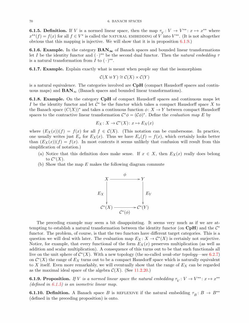
70 6. BANACH SPACES
6.1.5. Definition. If V is a normed linear space, then the map τV
: V → V ∗∗ : x 7→ x∗∗ wherex∗∗(f) = f(x) for all f ∈ V ∗ is called the natural embedding of V into V ∗∗. (It is not altogetherobvious that this mapping is injective. We will show that it is in proposition 6.1.9.)
6.1.6. Example. In the category BAN∞ of Banach spaces and bounded linear transformationslet I be the identity functor and ( · )∗∗ be the second dual functor. Then the natural embedding τis a natural transformation from I to ( · )∗∗.
6.1.7. Example. Explain exactly what is meant when people say that the isomorphism
C(X ] Y ) ∼= C(X)× C(Y )
is a natural equivalence. The categories involved are CpH (compact Hausdorff spaces and contin-uous maps) and BAN∞ (Banach spaces and bounded linear transformations).
6.1.8. Example. On the category CpH of compact Hausdorff spaces and continuous maps letI be the identity functor and let C∗ be the functor which takes a compact Hausdorff space X tothe Banach space (C(X))∗ and takes a continuous function φ : X → Y between compact Hausdorffspaces to the contractive linear transformation C∗φ = (Cφ)∗. Define the evaluation map E by
EX : X → C∗(X) : x 7→ EX(x)
where (EX(x))(f) = f(x) for all f ∈ C(X). (This notation can be cumbersome. In practice,one usually writes just Ex for EX(x). Thus we have Ex(f) = f(x), which certainly looks betterthan (EX(x))(f) = f(x). In most contexts it seems unlikely that confusion will result from thissimplification of notation.)
(a) Notice that this definition does make sense. If x ∈ X, then EX(x) really does belongto C∗(X).
(b) Show that the map E makes the following diagram commute
Xφ
//
EX
Y
EY
C∗(X)
C∗(φ)
// C∗(Y )
The preceding example may seem a bit disappointing. It seems very much as if we are at-tempting to establish a natural transformation between the identity functor (on CpH) and the C∗functor. The problem, of course, is that the two functors have different target categories. This is aquestion we will deal with later. The evaluation map EX : X → C∗(X) is certainly not surjective.Notice, for example, that every functional of the form EX(x) preserves multiplication (as well asaddition and scalar multiplication). A consequence of this turns out to be that such functionals alllive on the unit sphere of C∗(X). With a new topology (the so-called weak-star topology—see 6.2.7)on C∗(X) the range of EX turns out to be a compact Hausdorff space which is naturally equivalentto X itself. Even more remarkably, we will eventually show that the range of EX can be regardedas the maximal ideal space of the algebra C(X). (See 11.2.20.)
6.1.9. Proposition. If V is a normed linear space the natural embedding τV
: V → V ∗∗ : x 7→ x∗∗
(defined in 6.1.5) is an isometric linear map.
6.1.10. Definition. A Banach space B is reflexive if the natural embedding τB
: B → B∗∗
(defined in the preceding proposition) is onto.
6.2. ALAOGLU’S THEOREM 71
Example 6.1.6 shows that in the category of Banach spaces and bounded linear maps, themapping τ : B 7→ τ
Bis a natural transformation from the identity functor to the second dual
functor. Invoking the Hahn-Banach theorem we can say more.
6.1.11. Proposition. In the category of reflexive Banach spaces and bounded linear maps themapping τ : B 7→ τ
Bis a natural equivalence between the identity and second dual functors.
6.1.12. Example. Every Hilbert space is reflexive.
6.1.13. Exercise. Let V and W be normed linear spaces, U be a nonempty convex subset of V ,and f : U → W . Without using any form of the mean value theorem show that if df = 0 on U ,then f is constant on U . (For the definition of df , the differential of f , see sections 13.1–2 in mynotes [16].)
6.1.14. Example. Let l∞ be the Banach space of all bounded sequences of real numbers and c bethe subspace of l∞ comprising all sequences x = (xn) such that limn→∞ xn exists. Define
f : c→ R : x 7→ limn→∞
xn.
Then f is a continuous linear functional on c and ‖f‖ = 1. By the Hahn-Banach theorem f
has an extension to f ∈ l∞∗ with ‖f‖ = 1. For every subset A of N define a sequence(xAn)
by
xAn =
1, if n ∈ A;0, if n /∈ A.
Next define µ : P(N) → R : A 7→ f(xAn). Then µ is a finitely additive set
function but is not countably additive.
6.2. Alaoglu’s Theorem
6.2.1. Notation. Let V be a normed linear space, M ⊆ V , and F ⊆ V ∗. Then we define
M⊥ := f ∈ V ∗ : f(x) = 0 for all x ∈MF⊥ := x ∈ V : f(x) = 0 for all f ∈ F
One may read M⊥ as “M perp” or “M upper perp”; and F⊥ is “F perp” or “F lower perp”. Theset M⊥ is the annihilator of M and F⊥ is the pre-annihilator of F .
6.2.2. Proposition (Annihilators). Let B be a Banach space, M ⊆ B, and F ⊆ B∗. Then
(a) If M ⊆ N ⊆ B, then N⊥ ⊆M⊥.(b) If F ⊆ G ⊆ B∗, then G⊥ ⊆ F⊥.(c) M⊥ is a closed linear subspace of B∗.(d) F⊥ is a closed linear subspace of B.(e) M ⊆M⊥⊥.(f) F ⊆ F⊥⊥.(g) M⊥⊥ =
∨M .
(h) M⊥ = B∗ if and only if M = 0.(i) F⊥ = B if and only if F = 0.(j) If M is a linear subspace of B, then M⊥ = 0 if and only if M is dense in B.(k) If B is reflexive, then F⊥
⊥ =∨F .
Hint for proof . For (k) show that τ(F⊥) = F⊥ (where τ is the natural embedding) and thattherefore F⊥
⊥ = F⊥⊥.
6.2.3. Example. Let B be a Banach space that is not reflexive. Let F = ran τ (where τ is thenatural embedding). Then F⊥
⊥ = B∗∗ 6=∨F , so it is clear that (k) in the preceding proposition
need not hold in the nonreflexive case.
The next result is the Banach space analog of the fundamental theorem of linear algebra 1.2.42and proposition 5.2.25.
72 6. BANACH SPACES
6.2.4. Proposition. Let T ∈ B(B,C) where B and C are Banach spaces. Then
(a) kerT ∗ = (ranT )⊥.(b) kerT = (ranT ∗)⊥.
(c) ranT = (kerT ∗)⊥.
(d) ranT ∗ ⊆ (kerT )⊥.
6.2.5. Example. An example of a Banach space operator T for which ranT ∗ and (kerT )⊥ aredifferent is given in exercise 7, page 243 of [4].
The following example is of course a trivial consequence of proposition 3.3.8, but try to give asimple direct proof.
6.2.6. Example. The closed unit ball in l2 is not compact.
The usual norm topology on normed linear spaces turns out to be much too large for someapplications. As we have seen it has so many open sets that the closed unit ball is not compact(except in the finite dimensional case). On the other hand, too few open sets (the indiscretetopology, as an extreme example) would destroy duality theory by failing to provide a plentifulsupply of continuous linear functionals. The so-called weak-star topology (defined below) on thedual of a normed linear space turns out to be just the right size. It has enough open sets toguarantee a vigorous duality theory and few enough open sets to make the closed unit ball compact(see Alaoglu’s theorem 6.2.9).
6.2.7. Definition. Let V be a normed linear space. The weak topology on V is the weaktopology induced by the elements of V ∗. (So, of course, the weak topology on the dual space V ∗
is the weak topology induced by the elements of V ∗∗.) When a net (xλ) converges weakly to a
vector a in V we write xλw // a. The w∗-topology (pronounced weak star topology) on the dual
space V ∗ is the weak topology induced by the elements of ran τ where τ is the natural injection of
V into V ∗∗. When a net (fλ) converges weakly to a vector g in V ∗ we write fλw∗ // g. Notice
that when a Banach space B is reflexive (in particular, for Hilbert spaces) the weak and weak startopologies on B∗ are identical.
6.2.8. Proposition. Let f ∈ V ∗ where V is a Banach space. For every ε > 0 and every finitesubset F ⊆ V define
U(f ;F ; ε) = g ∈ V ∗ : |f(x)− g(x)| < ε for all x ∈ F.The family of all such sets is a base for the w∗-topology on V ∗.
The next result, Alaoglu’s theorem, asserting the w∗-compactness of the closed unit ball in thedual of a normed linear space V is one of the most useful theorems in functional analysis. Thus atfirst it may seem somewhat surprising that it is so hard to find a complete and carefully explainedproof of this result. The standard proof is in a sense very simple; it is basically just recognizingthat the members of a family F of scalar valued functions can be regarded either
(i) as functions defined on an uncountable product of compact subsets of the scalar field, oralternatively
(ii) as members of the closed unit ball of V ∗.
The crux of the proof is convincing yourself that the convergence of a net of such functions in theproduct space is exactly “the same thing” as its w∗-convergence in the closed unit ball of V ∗. Tryingsimultaneously to identify and distinguish between two sets of functions is notationally challenging.So my best advice is to work through it yourself until you see how ingenious, but basically simple,the argument is.
6.2.9. Theorem (Alaoglu’s theorem). The closed unit ball of a normed linear space is compact inthe w∗-topology.
6.3. THE OPEN MAPPING THEOREM 73
Hint for proof . Let V be a normed linear space and denote by [V ∗]1 the closed unit ball of itsdual space. For each x ∈ V define Dx = λ ∈ K : |λ| ≤ ‖x‖. The product P =
∏x∈V
Dx is compactby Tychonoff’s theorem. Consider the function
Φ: [V ∗]1 → P : f 7→(f(x)
)x∈V
where [V ∗]1 has the w∗-topology and P has the product topology (see 4.6.4). Here we have written(f(x)
)x∈V for the indexed family of numbers (or generalized sequence) rather than the more usual(
fx)x∈V . (For more on indexed families see [16], section 7.2.) It is easy to see that Φ is injective.
To show that it is continuous let(fλ)λ∈Λ
be a net in [V ∗]1 and g be a function in [V ∗]1 such
that fλw∗ // g. Notice that this happens if and only if πx(fλ) → πx(g) for every x ∈ V (where
πx is a coordinate projection on P—see 3.5.6). Finally, let(fλ)λ∈Λ
be a net in [V ∗]1 such that(Φ(fλ)
)λ∈Λ
converges in P. Show that the net(fλ(x)
)λ∈Λ
converges in K for every x ∈ V . Let
g(x) = limλfλ(x) for all x ∈ V and prove that g is linear, that ‖g‖ ≤ 1, that fλ
w∗ // g in [V ∗]1,
and that Φ(fλ)→ Φ(g) in P.
To the best of my knowledge the most reader-friendly version of this standard proof can befound in [5], Theorem 15.11. A much shorter, much easier notationally, much slicker, and muchless edifying proof is available in [41], theorem 2.5.2. I find it less edifying because of its reliance onuniversal nets. A net in a set S is universal if for every subset T of S the net is either eventuallyin T or eventually in its complement. Despite the fact that every net can be shown to have auniversal subnet, even to find a singe nontrivial example of a universal net (that is, one that is noteventually constant) requires the axiom of choice.
6.3. The Open Mapping Theorem
A question one can (and should) ask of any concrete category is whether every bijective mor-phism is necessarily an isomorphism. In some categories the answer is trivially yes (for example, inVEC). In other categories the answer is trivially no (in TOP, for example, consider the identitymap from the reals with the discrete topology to the reals with their usual topology). Frequentlyin categories which arise in studying analysis, algebra is tugging enthusiastically in one directionwhile topology is vigorously resisting, pulling in the other. Here the question can become quitefascinating—and the answer definitely nontrivial. In the category BAN∞ of Banach spaces andcontinuous linear maps, the question turns out to be intriguingly deep. In this case algebra prevails;the answer is affirmative. It turns out to be a direct consequence of the celebrated open mappingtheorem. Notice as you work through the following proof of this result that for the map in questioncompleteness of domain and completeness of codomain are both essential—and for quite differentreasons.
6.3.1. Definition. A mapping f : X → Y between topological spaces is open if it takes open setsto open sets; that is, f is an open mapping provided that f→(U) is open in Y whenever U is openin X.
The open mapping theorem says that continuous linear surjections between Banach spaces arealways open mappings. There is one technical detail that makes the proof of this result a bit tricky.Suppose that T is a continuous linear map from a Banach space B into a normed linear space Vand R is the image under T of an open ball around the origin in B. We will need to know thatif the closure of R contains some open ball about the origin in V , then R itself contains the sameball. It will be convenient to isolate this crucial bit of information in the next proposition.
6.3.2. Notation. In a normed linear space V we denote by (V )r the open ball about the origin inV of radius r.
74 6. BANACH SPACES
6.3.3. Proposition. Let T : B → V be a continuous linear map from a Banach space into a normed
linear space. If r, s > 0 and (V )s ⊆ T(
(B)r), then (V )s ⊆ T
((B)r
).
Hint for proof . First verify that without loss of generality we may assume that r = s = 1.
Thus our hypothesis is that (V )1 ⊆ T(
(B)1
).
Let z ∈ (V )1. The proof is complete if we can show that z ∈ T(
(B)1
). Choose δ > 0 such that
‖z‖ < 1− δ and let y = (1− δ)−1z. Construct a sequence (vk)∞k=0 of vectors in V which satisfy
(i) ‖y − vk‖ < δk for k = 0, 1, 2, . . . and(ii) vk − vk−1 ∈ T
(δk−1(B)1
)for k = 1, 2, 3, . . . .
To this end, start with v0 = 0. Use the hypothesis to conclude that y − v0 ∈ T(
(B)1
)and that
therefore there is a vector w0 ∈ T(
(B)1
)such that ‖(y − v0) − wo‖ < δ. Let v1 = v0 + w0 and
check that (i) and (ii) hold for k = 1.Then find w1 ∈ T
(δ(B)1
)so that ‖(y − v1) − w1‖ < δ2 and let v2 = v1 + w1. Check that (i)
and (ii) hold for k = 2. Proceed inductively.For each n ∈ N choose a vector un ∈ δn−1(B)1 such that T (un) = vn − vn−1. Show that the
sequence (un) is summable (use4.2.2) and let x =∑∞
n=1 un. Conclude the proof by showing thatTx = y and that z ∈ T
((B)1
).
6.3.4. Theorem (Open mapping theorem). Every bounded linear surjection between Banach spacesis an open mapping.
Hint for proof . Suppose that T : B → C is a bounded linear surjection between Banach spaces.Start by verifying the following claim: All we need to show is that T
((B)1
)contains an open ball
about the origin in C. Suppose for the moment we know that such a ball exists. Call it W . Givenan open subset U of B, we wish to show that its image under T is open in C. To this end take anarbitrary point y in T (U) and choose an x in U such that y = Tx. Since U − x is a neighborhoodof the origin in B, we can find a number r > 0 such that r (B)1 ⊆ U − x. Verify that T (U) is openby proving that y + rW ⊆ T (U).
To establish the claim above, let V = T((B)1
)and notice that since T is surjective, C =
T (B) =⋃∞k=1 kV . Use the version of the Baire category theorem which says that if a nonempty
complete metric space is the union of a sequence of closed sets, then at least one of these sets hasnonempty interior. (See, for example, Theorem 29.3.21 in[16].) Choose k ∈ N so that
(kV)o 6= ∅.
Thus there exists y ∈ V and r > 0 such that y+(C)r ⊆ kV . It is not hard to see from the convexityof kV that (C)r ⊆ kV . (Write an arbitrary point z in (C)r as 1
2(y + z) + 12(−y + z).) Now you
have (C)r/k ⊆ V . Use proposition 6.3.3.
6.3.5. Corollary. Every bounded linear bijection between Banach spaces is an isomorphism.
6.3.6. Corollary. Every bounded linear surjection between Banach spaces is a quotient map in BAN∞.
6.3.7. Example. Let Cu be the set of continuous real valued functions on [0, 1] under the uniform
norm and C1 be the same set of functions under the L1 norm ( ‖f‖1 =∫ 1
0 |f | dλ ). Then the identitymap I : Cu → C1 is a continuous linear bijection but is not open. (Why does this not contradict theopen mapping theorem?)
6.3.8. Example. Let l be the set of sequences of real numbers that are eventually zero, V be lequipped with the l1 norm, and W be l with the uniform norm. The identity map I : V →W is abounded linear bijection but is not an isomorphism.
6.3.9. Example. The mapping T : R2 → R : (x, y) 7→ x shows that although bounded linearsurjections between Banach spaces map open sets to open sets they need not map closed sets toclosed sets.
6.3.10. Proposition. Let V be a vector space and suppose that ‖·‖1 and ‖·‖2 are norms on Vwhose corresponding topologies are T1 and T2. If V is complete with respect to both norms and ifT1 ⊇ T2, then T1 = T2.
6.4. THE CLOSED GRAPH THEOREM 75
6.3.11. Exercise. Does there exist a sequence (an) of complex numbers satisfying the followingcondition: a sequence (xn) in C is absolutely summable if and only if (anxn) is bounded? Hint.Consider T : l∞ → l1 : (xn) 7→ (xn/an).
6.3.12. Example. Let C2([a, b]) be the family of all twice continuously differentiable real valuedfunctions on the interval [a, b]. Regard it as a vector space in the usual fashion. For each f ∈C2([a, b]) define
‖f‖ = ‖f‖u + ‖f ′‖u + ‖f ′′‖u .This is in fact a norm and under this norm C2([a, b]) is a Banach space.
6.3.13. Example. Let C2([a, b]) be the Banach space given in exercise 6.3.12, and p0 and p1 bemembers of C([a, b]). Define
T : C2([a, b])→ C([a, b]) : f 7→ f ′′ + p1f′ + p0f.
Then T is a bounded linear map.
6.3.14. Exercise. Consider a differential equation of the form
y′′ + p1 y′ + p0 y = q (∗)
where p0, p1, and q are (fixed) continuous real valued functions on the interval [a, b]. Make precise,and prove, the assertion that the solutions to (∗) depend continuously on the initial values. Youmay use without proof a standard theorem: For every point c in [a, b] and every pair of real numbersa0 and a1, there exists a unique solution of (∗) such that y(c) = a0 and y′(c) = a1. Hint. For afixed c ∈ [a, b] consider the map
S : C2([a, b])→ C([a, b])× R2 : f 7→(Tf, f(c), f ′(c)
)where C2([a, b]) is the Banach space of example 6.3.12 and T is the bounded linear map of exam-ple 6.3.13.
6.3.15. Definition. An bounded linear map T : V →W between normed linear spaces is boundedaway from zero (or bounded below) if there exists a number δ > 0 such that ‖Tx‖ ≥ δ‖x‖ forall x ∈ V . (Recall that the word “bounded” means one thing when modifying a linear map andand something quite different when applied to a general function; so does the expression “boundedaway from zero”. See definition 5.2.26.)
6.3.16. Proposition. A bounded linear map between Banach spaces is bounded away from zero ifand only if it has closed range and zero kernel.
6.4. The Closed Graph Theorem
A simple necessary and sufficient condition for a linear map T : B → C between Banach spacesto be continuous is that its graph be closed. In one direction this is almost obvious. The converseis called the closed graph theorem. When we ask for the graph of T to be “closed” we mean closedas a subset of B×C with the product topology. Recall (from 4.6.8) that the topology on the directsum B ⊕ C induced by the product norm is the same as the product topology on B × C.
6.4.1. Exercise. If T : B → C is a continuous linear map between Banach spaces, then its graphis closed.
6.4.2. Theorem (Closed graph theorem). Let T : B → C be a linear map between Banach spaces.If the graph of T is closed, then T is continuous.
Hint for proof. Let G = (x, Tx) : x ∈ B be the graph of T . Apply (corollary 6.3.5 of) theopen mapping theorem to the map
π : G→ B : (x, Tx) 7→ x .
76 6. BANACH SPACES
The next proposition gives a very simple necessary and sufficient condition for the graph of alinear map between Banach spaces to be closed.
6.4.3. Proposition. Let T : B → C be a linear mapping between Banach spaces. Then T iscontinuous if and only if the following condition is satisfied:
if xn → 0 in B and Txn → c in C, then c = 0.
6.4.4. Proposition. Suppose T : B → C is a linear map between Banach spaces such that if xn → 0in B then (g T )(xn)→ 0 for every g ∈ C∗. Then T is bounded.
6.4.5. Proposition. Let T : B → C be a linear function between Banach spaces. Define T ∗f = fTfor every f ∈ C∗. If T ∗ maps C∗ into B∗, then T is continuous.
6.4.6. Definition. A linear map T from a vector space into itself is idempotent if T 2 = T .
6.4.7. Proposition. An idempotent linear map from a Banach space into itself is continuous ifand only if it has closed kernel and range.
Hint for proof . For the “if” part, use proposition 6.4.3.
The next proposition is a useful application of the closed graph theorem to Hilbert space oper-ators.
6.4.8. Proposition. Let H be a Hilbert space and S and T be functions from H into itself suchthat
〈Sx, y〉 = 〈x, Ty〉for all x, y ∈ H. Then S and T are bounded linear operators.
Hint for proof . To verify the linearity of the map S consider the inner product of the vectorsS(αx + βy) − αSx − βSy and z, where x, y, z ∈ H and α, β ∈ K. To establish the continuity ofS, show that its graph is closed.
Recall that in the preceding proposition the operator T is the (Hilbert space) adjoint of S; thatis, T = S∗.
6.4.9. Definition. Let a < b in R. A function f : [a, b] → R is continuously differentiable if it isdifferentiable on (an open set containing) [a, b] and its derivative f ′ is continuous on [a, b]. The setof all continuously differentiable real valued functions on [a, b] is denoted by C1( [a, b] ).
6.4.10. Example. Let D : C1( [0, 1] ) → C( [0, 1] ) : f 7→ f ′ where both C1( [0, 1] ) and C( [0, 1] )are equipped with the uniform norm. The mapping D is linear and has closed graph but is notcontinuous. (Why does this not contradict the closed graph theorem? What can we concludeabout C1( [0, 1] )?)
6.4.11. Proposition. Suppose that S : A → B and T : B → C are linear maps between Banachspaces and that T is bounded and injective. Then S is bounded if and only if TS is.
6.5. Banach Space Duality
6.5.1. Convention. In the context of Banach spaces we adopt the same convention for the useof the word “subspace” we used for Hilbert spaces. The word “subspace” will always mean closedvector subspace. To indicate that M is a subspace of a Banach space B we write M 4 B.
6.5.2. Proposition. If M is a subspace of a Banach space B, then the quotient normed linearspace B/M is also a Banach space.
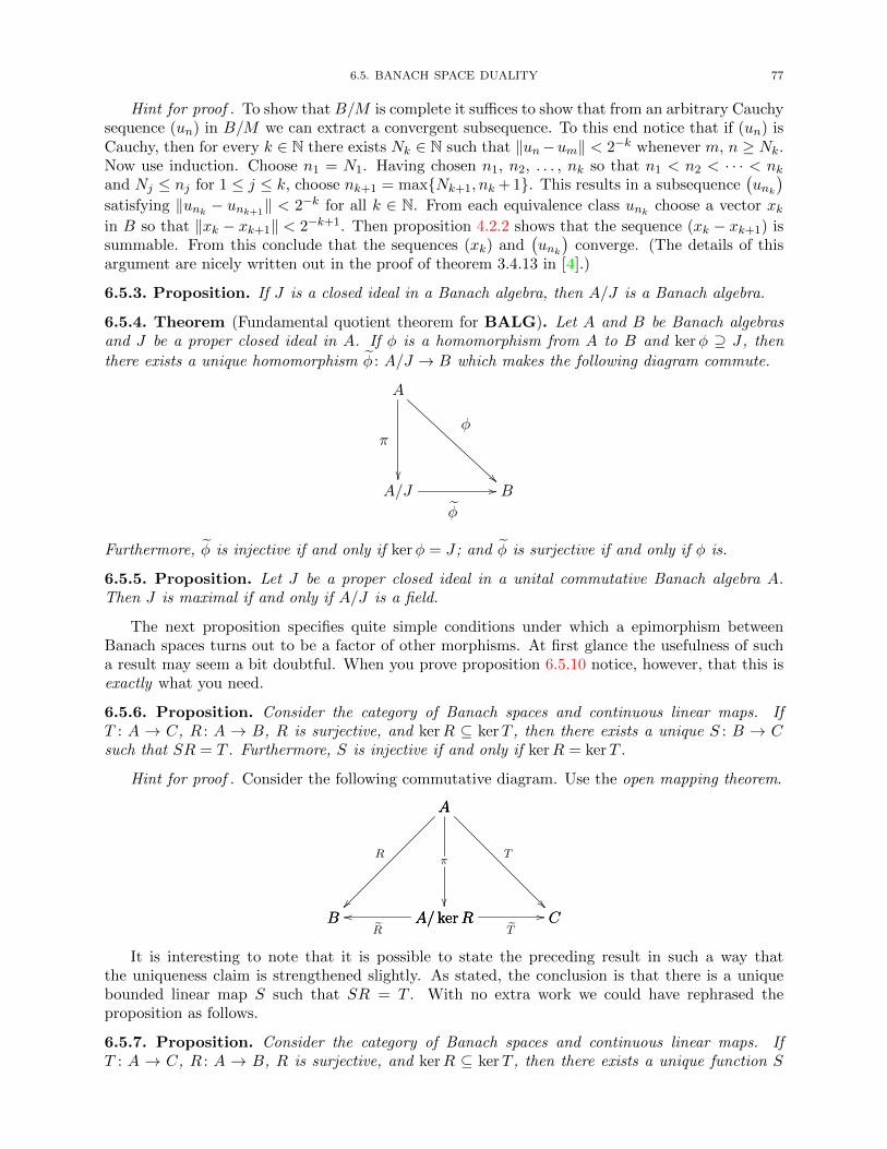
6.5. BANACH SPACE DUALITY 77
Hint for proof . To show that B/M is complete it suffices to show that from an arbitrary Cauchysequence (un) in B/M we can extract a convergent subsequence. To this end notice that if (un) isCauchy, then for every k ∈ N there exists Nk ∈ N such that ‖un−um‖ < 2−k whenever m, n ≥ Nk.Now use induction. Choose n1 = N1. Having chosen n1, n2, . . . , nk so that n1 < n2 < · · · < nkand Nj ≤ nj for 1 ≤ j ≤ k, choose nk+1 = maxNk+1, nk + 1. This results in a subsequence
(unk)
satisfying ‖unk − unk+1‖ < 2−k for all k ∈ N. From each equivalence class unk choose a vector xk
in B so that ‖xk − xk+1‖ < 2−k+1. Then proposition 4.2.2 shows that the sequence (xk − xk+1) issummable. From this conclude that the sequences (xk) and
(unk)
converge. (The details of thisargument are nicely written out in the proof of theorem 3.4.13 in [4].)
6.5.3. Proposition. If J is a closed ideal in a Banach algebra, then A/J is a Banach algebra.
6.5.4. Theorem (Fundamental quotient theorem for BALG). Let A and B be Banach algebrasand J be a proper closed ideal in A. If φ is a homomorphism from A to B and kerφ ⊇ J , then
there exists a unique homomorphism φ : A/J → B which makes the following diagram commute.
A
π
φ
A/J
φ
// B
Furthermore, φ is injective if and only if kerφ = J ; and φ is surjective if and only if φ is.
6.5.5. Proposition. Let J be a proper closed ideal in a unital commutative Banach algebra A.Then J is maximal if and only if A/J is a field.
The next proposition specifies quite simple conditions under which a epimorphism betweenBanach spaces turns out to be a factor of other morphisms. At first glance the usefulness of sucha result may seem a bit doubtful. When you prove proposition 6.5.10 notice, however, that this isexactly what you need.
6.5.6. Proposition. Consider the category of Banach spaces and continuous linear maps. IfT : A → C, R : A → B, R is surjective, and kerR ⊆ kerT , then there exists a unique S : B → Csuch that SR = T . Furthermore, S is injective if and only if kerR = kerT .
Hint for proof . Consider the following commutative diagram. Use the open mapping theorem.
B A/ kerRooR
A/ kerR CT
//
A
B
R
A
A/ kerR
π
A
C
T
It is interesting to note that it is possible to state the preceding result in such a way thatthe uniqueness claim is strengthened slightly. As stated, the conclusion is that there is a uniquebounded linear map S such that SR = T . With no extra work we could have rephrased theproposition as follows.
6.5.7. Proposition. Consider the category of Banach spaces and continuous linear maps. IfT : A → C, R : A → B, R is surjective, and kerR ⊆ kerT , then there exists a unique function S
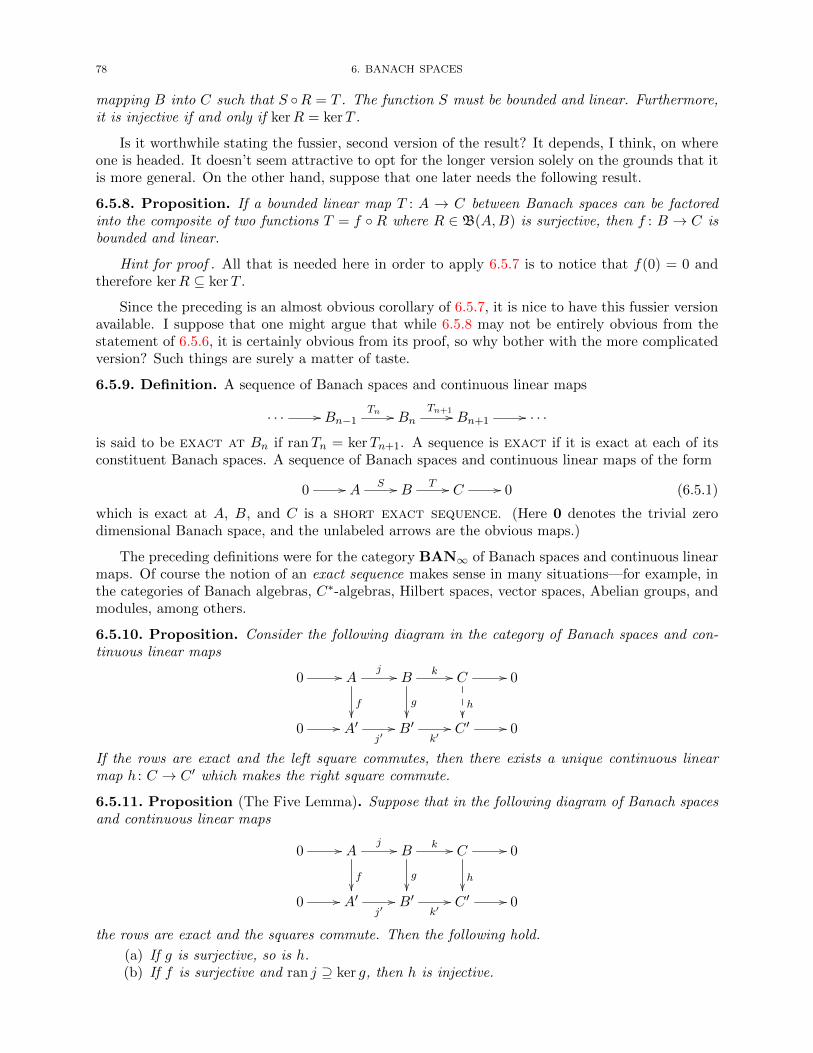
78 6. BANACH SPACES
mapping B into C such that S R = T . The function S must be bounded and linear. Furthermore,it is injective if and only if kerR = kerT .
Is it worthwhile stating the fussier, second version of the result? It depends, I think, on whereone is headed. It doesn’t seem attractive to opt for the longer version solely on the grounds that itis more general. On the other hand, suppose that one later needs the following result.
6.5.8. Proposition. If a bounded linear map T : A → C between Banach spaces can be factoredinto the composite of two functions T = f R where R ∈ B(A,B) is surjective, then f : B → C isbounded and linear.
Hint for proof . All that is needed here in order to apply 6.5.7 is to notice that f(0) = 0 andtherefore kerR ⊆ kerT .
Since the preceding is an almost obvious corollary of 6.5.7, it is nice to have this fussier versionavailable. I suppose that one might argue that while 6.5.8 may not be entirely obvious from thestatement of 6.5.6, it is certainly obvious from its proof, so why bother with the more complicatedversion? Such things are surely a matter of taste.
6.5.9. Definition. A sequence of Banach spaces and continuous linear maps
· · · // Bn−1Tn // Bn
Tn+1 // Bn+1// · · ·
is said to be exact at Bn if ranTn = kerTn+1. A sequence is exact if it is exact at each of itsconstituent Banach spaces. A sequence of Banach spaces and continuous linear maps of the form
0 // AS // B
T // C // 0 (6.5.1)
which is exact at A, B, and C is a short exact sequence. (Here 0 denotes the trivial zerodimensional Banach space, and the unlabeled arrows are the obvious maps.)
The preceding definitions were for the category BAN∞ of Banach spaces and continuous linearmaps. Of course the notion of an exact sequence makes sense in many situations—for example, inthe categories of Banach algebras, C∗-algebras, Hilbert spaces, vector spaces, Abelian groups, andmodules, among others.
6.5.10. Proposition. Consider the following diagram in the category of Banach spaces and con-tinuous linear maps
0 // A
f
j // B
g
k // C
h
// 0
0 // A′j′// B′
k′// C ′ // 0
If the rows are exact and the left square commutes, then there exists a unique continuous linearmap h : C → C ′ which makes the right square commute.
6.5.11. Proposition (The Five Lemma). Suppose that in the following diagram of Banach spacesand continuous linear maps
0 // A
f
j // B
g
k // C
h
// 0
0 // A′j′// B′
k′// C ′ // 0
the rows are exact and the squares commute. Then the following hold.
(a) If g is surjective, so is h.(b) If f is surjective and ran j ⊇ ker g, then h is injective.
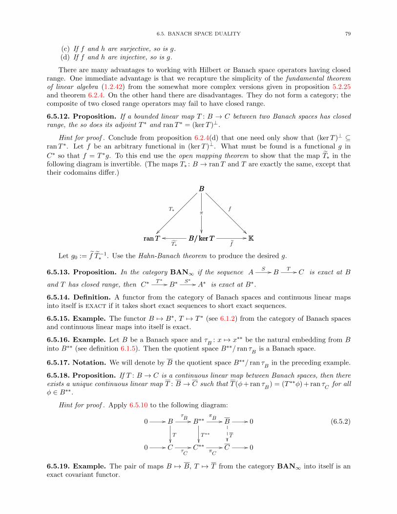
6.5. BANACH SPACE DUALITY 79
(c) If f and h are surjective, so is g.(d) If f and h are injective, so is g.
There are many advantages to working with Hilbert or Banach space operators having closedrange. One immediate advantage is that we recapture the simplicity of the fundamental theoremof linear algebra (1.2.42) from the somewhat more complex versions given in proposition 5.2.25and theorem 6.2.4. On the other hand there are disadvantages. They do not form a category; thecomposite of two closed range operators may fail to have closed range.
6.5.12. Proposition. If a bounded linear map T : B → C between two Banach spaces has closedrange, the so does its adjoint T ∗ and ranT ∗ = (kerT )⊥.
Hint for proof . Conclude from proposition 6.2.4(d) that one need only show that (kerT )⊥ ⊆ranT ∗. Let f be an arbitrary functional in (kerT )⊥. What must be found is a functional g in
C∗ so that f = T ∗g. To this end use the open mapping theorem to show that the map T∗ in thefollowing diagram is invertible. (The maps T∗ : B → ranT and T are exactly the same, except thattheir codomains differ.)
ranT B/ kerTooT∗
B/ kerT Kf
//
B
ranT
T∗
B
B/ kerT
π
B
K
f
Let g0 := f T−1∗ . Use the Hahn-Banach theorem to produce the desired g.
6.5.13. Proposition. In the category BAN∞ if the sequence AS // B
T // C is exact at B
and T has closed range, then C∗T ∗ // B∗
S∗ // A∗ is exact at B∗.
6.5.14. Definition. A functor from the category of Banach spaces and continuous linear mapsinto itself is exact if it takes short exact sequences to short exact sequences.
6.5.15. Example. The functor B 7→ B∗, T 7→ T ∗ (see 6.1.2) from the category of Banach spacesand continuous linear maps into itself is exact.
6.5.16. Example. Let B be a Banach space and τB
: x 7→ x∗∗ be the natural embedding from Binto B∗∗ (see definition 6.1.5). Then the quotient space B∗∗/ ran τ
Bis a Banach space.
6.5.17. Notation. We will denote by B the quotient space B∗∗/ ran τB
in the preceding example.
6.5.18. Proposition. If T : B → C is a continuous linear map between Banach spaces, then thereexists a unique continuous linear map T : B → C such that T (φ+ ran τ
B) = (T ∗∗φ) + ran τ
Cfor all
φ ∈ B∗∗.
Hint for proof . Apply 6.5.10 to the following diagram:
0 // B
T
τB // B∗∗
T ∗∗
πB // B
T
// 0
0 // C τC
// C∗∗ πC
// C // 0
(6.5.2)
6.5.19. Example. The pair of maps B 7→ B, T 7→ T from the category BAN∞ into itself is anexact covariant functor.
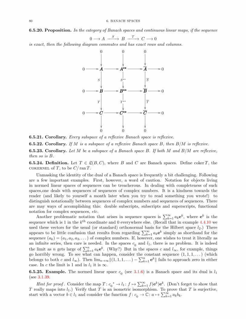
80 6. BANACH SPACES
6.5.20. Proposition. In the category of Banach spaces and continuous linear maps, if the sequence
0 −→ AS−−−−→ B
T−−−−→ C −→ 0
is exact, then the following diagram commutes and has exact rows and columns.
C C∗∗//C0 // C
0
C∗∗ C//C∗∗
0
C
0
C 0//
B 0//B∗∗ B//B B∗∗//B0 //
A A∗∗//A0 // A
0
A∗∗ A//A∗∗
0
A
0
A 0//A
B
S
A∗∗
B∗∗
S∗∗
A
B
S
B
C
T
B∗∗
C∗∗
T ∗∗
B
C
T
6.5.21. Corollary. Every subspace of a reflexive Banach space is reflexive.
6.5.22. Corollary. If M is a subspace of a reflexive Banach space B, then B/M is reflexive.
6.5.23. Corollary. Let M be a subspace of a Banach space B. If both M and B/M are reflexive,then so is B.
6.5.24. Definition. Let T ∈ L(B,C), where B and C are Banach spaces. Define cokerT , thecokernel of T , to be C/ ranT .
Unmasking the identity of the dual of a Banach space is frequently a bit challenging. Followingare a few important examples. First, however, a word of caution. Notation for objects livingin normed linear spaces of sequences can be treacherous. In dealing with completeness of suchspaces,one deals with sequences of sequences of complex numbers. It is a kindness towards thereader (and likely to yourself a month later when you try to read something you wrote!) todistinguish notationally between sequences of complex numbers and sequences of sequences. Thereare may ways of accomplishing this: double subscripts, subscripts and superscripts, functionalnotation for complex sequences, etc.
Another problematic notation that arises in sequence spaces is∑∞
k=1 akek, where ek is the
sequence which is 1 in the kth coordinate and 0 everywhere else. (Recall that in example 4.4.10 weused these vectors for the usual (or standard) orthonormal basis for the Hilbert space l2.) Thereappears to be little confusion that results from regarding
∑∞k=1 ake
k simply as shorthand for thesequence (ak) = (a1, a2, a3, . . . ) of complex numbers. If, however, one wishes to treat it literally asan infinite series, then care is needed. In the spaces c
0and l1, there is no problem. It is indeed
the limit as n gets large of∑n
k=1 akek. (Why?) But in the spaces c and l∞, for example, things
go horribly wrong. To see what can happen, consider the constant sequence (1, 1, 1, . . . ) (whichbelongs to both c and l∞). Then limn→∞‖(1, 1, 1, . . . )−
∑nk=1 ek‖ fails to approach zero in either
case. In c the limit is 1 and in l1 it is ∞.
6.5.25. Example. The normed linear space c0
(see 3.1.6) is a Banach space and its dual is l1(see 3.1.39.
Hint for proof . Consider the map T : c0∗ → l1 : f 7→
∑∞k=1 f(ek)ek. (Don’t forget to show that
T really maps into l1.) Verify that T is an isometric isomorphism. To prove that T is surjective,start with a vector b ∈ l1 and consider the function f : c
0→ C : a 7→
∑∞k=1 akbk.
6.5. BANACH SPACE DUALITY 81
6.5.26. Corollary. The space l1 is a Banach space.
It is interesting that, as it turns out, the spaces c0
and c are not isometrically isomorphic, eventhough their dual spaces are. The computation of the dual of c is technically slightly fussier thanthe one for c
0∗. It may be helpful to consider the Schauder bases for these two spaces.
6.5.27. Definition. A sequence (ek) of vectors in a Banach space is a Schauder basis for thespace if for every x ∈ B there exists a unique sequence (αk) of scalars such that x =
∑∞k=1 αke
k.
Two comments about the preceding definition: The word “unique” is very important; and it isnot true that every Banach space has a Schauder basis.
6.5.28. Example. An orthonormal basis in a separable Hilbert space is a Schauder basis for thespace. (See propositions 4.4.12 and 4.4.17.)
6.5.29. Example. We choose the standard (or usual) basis vectors for c0
in the same way
as for l2 (see 4.4.10). For each n ∈ N let en be the sequence in l2 whose nth coordinate is 1 and allthe other coordinates are 0. Then en : n ∈ N is a Schauder basis for c
0.
At first glance the space c of all convergent sequences may seem enormously larger than c0,
which contains only those sequences which converge to zero. After all, corresponding to each vectorx in c
0there are uncountably many distinct vectors in c (just add any nonzero complex number to
each term of the sequence x). Is it possible for c, containing, as it does, uncountably many copiesof the uncountable collection of members of c
0, to have a (necessarily countable) Schauder basis?
The answer, upon reflection, is yes. All we need to do is add a single element to the basis for c0
todeal with the translations.
6.5.30. Example. Let e1, e2, . . . be as in the preceding example 6.5.29. Also denote by 1 theconstant sequence (1, 1, 1, . . . ) in c. Then (1, e1, e2, . . . ) is a Schauder basis for c.
6.5.31. Example. The normed linear space c (see 3.1.5) is a Banach space and its dual is l1(see 3.1.39).
Hint for proof . Observe initially that for every f ∈ c∗ the sequence(f(ek)
)is absolutely sum-
mable and that as a consequence∑∞
k=1 akf(ek) converges for every sequence a = (a1, a2, . . . ) in c.
Also note that each a ∈ c can be written as a = a∞1 +∑∞
k=1(ak − a∞)ek where a∞ := limk→∞ akand let 1 := (1, 1, 1, . . . ). Use this to prove that for every f ∈ c∗
|f(a)| ≤[|βf |+
∞∑k=1
|f(ek)|]‖a‖∞
where βf := f(1)−∑∞
k=1 f(ek). For t = (t0, t1, t2, . . . ) ∈ l1 and a = (a1, a2, a3, . . . ) ∈ c define
St(a) := t0a∞ +∞∑k=1
tkak
and verify that S : t 7→ St is a continuous linear map from l1 into c∗. Next, for f ∈ c∗ define
Tf := (βf , f(e1), f(e2), . . . )
and show that T : f 7→ Tf is a linear isometry from c∗ into l1. Now in order to see that c∗ and l1are isometrically isomorphic all that is needed is to show that ST = idc∗ and TS = idl1 .
6.5.32. Definition. A topological space is locally compact if every point of the space has acompact neighborhood.
6.5.33. Notation. Let X be a locally compact space. A scalar valued function f on X belongs toC0(X) if it is continuous and vanishes at infinity (that is, if for every number ε > 0 there exists acompact subset of X outside of which |f(x)| < ε).
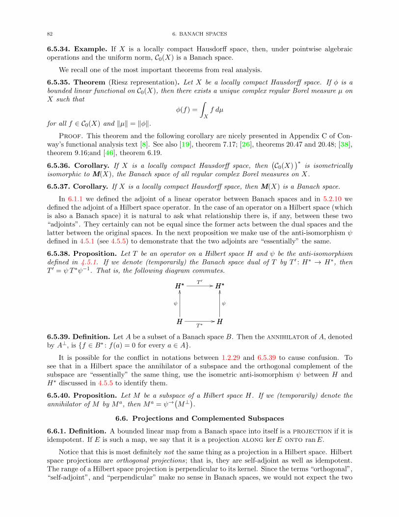
82 6. BANACH SPACES
6.5.34. Example. If X is a locally compact Hausdorff space, then, under pointwise algebraicoperations and the uniform norm, C0(X) is a Banach space.
We recall one of the most important theorems from real analysis.
6.5.35. Theorem (Riesz representation). Let X be a locally compact Hausdorff space. If φ is abounded linear functional on C0(X), then there exists a unique complex regular Borel measure µ onX such that
φ(f) =
∫Xf dµ
for all f ∈ C0(X) and ‖µ‖ = ‖φ‖.
Proof. This theorem and the following corollary are nicely presented in Appendix C of Con-way’s functional analysis text [8]. See also [19], theorem 7.17; [26], theorems 20.47 and 20.48; [38],theorem 9.16;and [46], theorem 6.19.
6.5.36. Corollary. If X is a locally compact Hausdorff space, then(C0(X)
)∗is isometrically
isomorphic to M(X), the Banach space of all regular complex Borel measures on X.
6.5.37. Corollary. If X is a locally compact Hausdorff space, then M(X) is a Banach space.
In 6.1.1 we defined the adjoint of a linear operator between Banach spaces and in 5.2.10 wedefined the adjoint of a Hilbert space operator. In the case of an operator on a Hilbert space (whichis also a Banach space) it is natural to ask what relationship there is, if any, between these two“adjoints”. They certainly can not be equal since the former acts between the dual spaces and thelatter between the original spaces. In the next proposition we make use of the anti-isomorphism ψdefined in 4.5.1 (see 4.5.5) to demonstrate that the two adjoints are “essentially” the same.
6.5.38. Proposition. Let T be an operator on a Hilbert space H and ψ be the anti-isomorphismdefined in 4.5.1. If we denote (temporarily) the Banach space dual of T by T ′ : H∗ → H∗, thenT ′ = ψ T ∗ψ−1. That is, the following diagram commutes.
H HT ∗
//
H∗
H
OO
ψ
H∗ H∗T ′ // H∗
H
OO
ψ
6.5.39. Definition. Let A be a subset of a Banach space B. Then the annihilator of A, denotedby A⊥, is f ∈ B∗ : f(a) = 0 for every a ∈ A.
It is possible for the conflict in notations between 1.2.29 and 6.5.39 to cause confusion. Tosee that in a Hilbert space the annihilator of a subspace and the orthogonal complement of thesubspace are “essentially” the same thing, use the isometric anti-isomorphism ψ between H andH∗ discussed in 4.5.5 to identify them.
6.5.40. Proposition. Let M be a subspace of a Hilbert space H. If we (temporarily) denote theannihilator of M by Ma, then Ma = ψ→
(M⊥
).
6.6. Projections and Complemented Subspaces
6.6.1. Definition. A bounded linear map from a Banach space into itself is a projection if it isidempotent. If E is such a map, we say that it is a projection along kerE onto ranE.
Notice that this is most definitely not the same thing as a projection in a Hilbert space. Hilbertspace projections are orthogonal projections; that is, they are self-adjoint as well as idempotent.The range of a Hilbert space projection is perpendicular to its kernel. Since the terms “orthogonal”,“self-adjoint”, and “perpendicular” make no sense in Banach spaces, we would not expect the two
6.6. PROJECTIONS AND COMPLEMENTED SUBSPACES 83
notions of “projection” to be identical. In both cases, however, the projections are bounded, linear,and idempotent.
6.6.2. Definition. Let M be a closed linear subspace of a Banach space B. If there exists aclosed linear subspace N of B such that B = M ⊕ N , then we say that M is a complementedsubspace, that N is its (Banach space) complement, and that the subspaces M and N arecomplementary.
6.6.3. Proposition. Let M and N be complementary subspaces of a Banach space B. Clearly,each element in B can be written uniquely in the form m+ n for some m ∈M and n ∈ N . Definea mapping E : B → B by E(m + n) = m for m ∈ M and n ∈ N . Then E is the projection alongN onto M .
Hint for proof . Use 6.4.7.
6.6.4. Proposition. If E is a projection on a Banach space B, then its kernel and range arecomplementary subspaces of B.
The following is an obvious corollary of the two preceding propositions
6.6.5. Corollary. A subspace of a Banach space is complemented if and only if it is the range ofa projection.
6.6.6. Proposition. Let B be a Banach space. If E : B → B is a projection onto a subspace Malong a subspace N , then I − E is a projection onto N along M .
6.6.7. Proposition. If M and N are complementary subspaces of a Banach space B, then B/Mand N are isomorphic.
6.6.8. Proposition. Let T : B → C be a bounded linear map between Banach spaces. If T isinjective and ranT is complemented, then T has a left inverse.
Hint for proof . For this hint we introduce a (somewhat fussy) notation. If f : X → Y is afunction between two sets, we define f• : X → ran f : x 7→ f(x). That is, f• is exactly the samefunction as f , except that its codomain is the range of f .
Since ranT is complemented there exists a projection E from C onto ranT (by 6.6.5). Showthat T• has a continuous inverse. Let S = T•
−1E•.
6.6.9. Proposition. Let S : C → B be a bounded linear map between Banach spaces. If S issurjective and kerS is complemented, then S has a right inverse.
Hint for proof . Since kerS is complemented there exists N C such that C = N ⊕ kerS.Show that the restriction of S to N has a continuous inverse and compose this inverse with theinclusion mapping of N into C.
The next result serves as a converse to both propositions 6.6.8 and 6.6.9.
6.6.10. Proposition. Let T : B → C and S : C → B be bounded linear maps between Banachspaces. If ST = idB, then
(a) S is surjective;(b) T is injective;(c) TS is a projection along kerS onto ranT ; and(d) C = ranT ⊕ kerS.
6.6.11. Proposition. If in the category BAN∞ the sequences
0 −−−−→ Aj−−−−→ B
f−−−−→ C −−−−→ 0and
0 −−−−→ Cg−−−−→ B
p−−−−→ D −−−−→ 0are exact and if fg = idC , then pj is an isomorphism from A onto D.
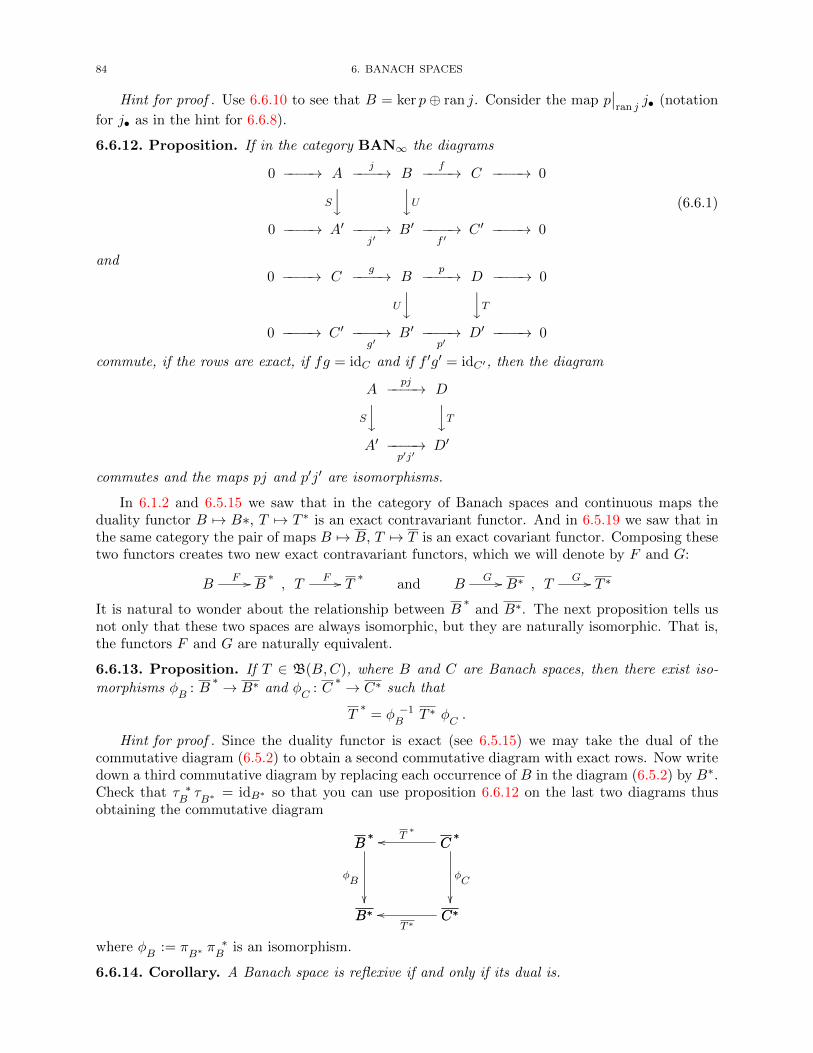
84 6. BANACH SPACES
Hint for proof . Use 6.6.10 to see that B = ker p⊕ ran j. Consider the map p∣∣ran j
j• (notation
for j• as in the hint for 6.6.8).
6.6.12. Proposition. If in the category BAN∞ the diagrams
0 −−−−→ Aj−−−−→ B
f−−−−→ C −−−−→ 0
S
y yU0 −−−−→ A′ −−−−→
j′B′ −−−−→
f ′C ′ −−−−→ 0
(6.6.1)
and0 −−−−→ C
g−−−−→ Bp−−−−→ D −−−−→ 0
U
y yT0 −−−−→ C ′ −−−−→
g′B′ −−−−→
p′D′ −−−−→ 0
commute, if the rows are exact, if fg = idC and if f ′g′ = idC′, then the diagram
Apj−−−−→ D
S
y yTA′ −−−−→
p′j′D′
commutes and the maps pj and p′j′ are isomorphisms.
In 6.1.2 and 6.5.15 we saw that in the category of Banach spaces and continuous maps theduality functor B 7→ B∗, T 7→ T ∗ is an exact contravariant functor. And in 6.5.19 we saw that inthe same category the pair of maps B 7→ B, T 7→ T is an exact covariant functor. Composing thesetwo functors creates two new exact contravariant functors, which we will denote by F and G:
BF // B
∗, T
F // T∗
and BG // B∗ , T
G // T ∗
It is natural to wonder about the relationship between B∗
and B∗. The next proposition tells usnot only that these two spaces are always isomorphic, but they are naturally isomorphic. That is,the functors F and G are naturally equivalent.
6.6.13. Proposition. If T ∈ B(B,C), where B and C are Banach spaces, then there exist iso-
morphisms φB
: B∗ → B∗ and φ
C: C∗ → C∗ such that
T∗
= φB−1 T ∗ φ
C.
Hint for proof . Since the duality functor is exact (see 6.5.15) we may take the dual of thecommutative diagram (6.5.2) to obtain a second commutative diagram with exact rows. Now writedown a third commutative diagram by replacing each occurrence of B in the diagram (6.5.2) by B∗.Check that τ
B∗ τ
B∗= idB∗ so that you can use proposition 6.6.12 on the last two diagrams thus
obtaining the commutative diagram
B∗ C∗ooT ∗
B∗
B∗
φB
B∗
C∗oo T
∗
C∗
C∗
φC
where φB
:= πB∗πB∗ is an isomorphism.
6.6.14. Corollary. A Banach space is reflexive if and only if its dual is.
6.7. THE PRINCIPLE OF UNIFORM BOUNDEDNESS 85
6.6.15. Proposition. Every finite dimensional subspace of a Banach space is complemented.
Hint for proof . Let F be a finite dimensional subspace of a Banach space B and let e1, . . . , enbe a Hamel basis for F . Then for each x ∈ F there exist unique scalars α1(x), . . . , αn(x) such thatx =
∑nk=1 αk(x)ek. For each 1 ≤ k ≤ n verify that αk is a bounded linear functional, which can
be extended to all of B. Let N be the intersection of the kernels of these extensions and show thatB = F ⊕N .
6.6.16. Definition. Recall that in 1.1.15 we defined the codimension of a subspace of a vectorspace as the dimension of its vector space complement (which always exists by proposition 1.1.18).We adopt the same language for Banach spaces: the codimension of any vector subspace of aBanach space is the dimension of its vector space complement.
For the following corollary (of proposition 6.6.15) keep in mind the convention 6.5.1 on the useof the word “subspace” in the context of Banach spaces.
6.6.17. Corollary. In a Banach space every subspace of finite codimension is complemented.
Let M be a nonzero subspace of a Banach space M . Consider the following two properties ofthe pair B and M .
Property P: There exists a projection of norm 1 from B onto M .Property E: For every Banach space C, every bounded linear map from M to C can be extended
to a bounded linear map from B to C without increasing its norm.
6.6.18. Proposition. For a nonzero subspace M of a Banach space B, properties P and E areequivalent.
Hint for proof . To show that E implies P start by extending the identity map on M to allof B.
6.7. The Principle of Uniform Boundedness
6.7.1. Definition. Let S be a set and V be a normed linear space. A family F of functions fromS into V is pointwise bounded if for every x ∈ S there exists a constant Mx > 0 such that‖f(x)‖ ≤Mx for every f ∈ F .
6.7.2. Definition. Let V and W be normed linear spaces. A family T of bounded linear mapsfrom V into W is uniformly bounded if there exists M > 0 such that ‖T‖ ≤M for every T ∈ T .
6.7.3. Exercise. Let V and W be normed linear spaces. If a family T of bounded linear mapsfrom V into W is uniformly bounded, then it is pointwise bounded.
The principle of uniform boundedness is the assertion that the converse of 6.7.3 holds wheneverV is complete. To prove this we will make use of a “local” analog of this for continuous functionson a complete metric space. It says, roughly, that if a family of real valued functions on a completemetric space is pointwise bounded then it is uniformly bounded on some nonempty open subset ofthe space.
6.7.4. Proposition. Let M be a complete metric space and F ⊆ C(M,R). If for every x ∈ Mthere exists a constant Nx > 0 such that |f(x)| ≤ Nx for every f ∈ F , then there exists a nonemptyopen set U in M and a number N > 0 such that |f(u)| ≤ N for every f ∈ F and every u ∈ U .
Hint for proof . For each natural number k let Ak =⋂f←
([−k, k]
): f ∈ F. Use the same
version of the Baire category theorem we used in proving the open mapping theorem (6.3.4) toconclude that for at least one n ∈ N the set An has nonempty interior. Let U = An
.
6.7.5. Theorem (Principle of uniform boundedness). Let B be a Banach space and W be a normedlinear space. If a family T of bounded linear maps from B into W is pointwise bounded, then it isuniformly bounded.
86 6. BANACH SPACES
Hint for proof . For every T ∈ T define
fT
: B → R : x 7→ ‖Tx‖.Use the preceding proposition to show that there exist a nonempty open subset U of B and aconstant M > 0 such that f
T(x) ≤ M for every T ∈ T and every x ∈ U . Choose a point a ∈ B
and a number r > 0 so that Br(a) ⊆ U . Then verify that
‖Ty‖ ≤ r−1(fT
(a+ ry) + fT
(a))≤ 2Mr−1
for every T ∈ T and every y ∈ B such that ‖y‖ ≤ 1.
6.7.6. Theorem (Banach-Steinhaus). Let B be a Banach space, W be a normed linear space, and(Tn) be a sequence of bounded linear maps from B into W . If the pointwise limit limn→∞ Tnx existsfor every x in B, then the map S : B →W : x 7→ limn→∞ Tnx is a bounded linear transformation.
Hint for proof . For every x ∈ B the sequence(‖Tnx‖
)∞n=1
is convergent, therefore bounded.Use 6.7.5.
6.7.7. Definition. A subset A of a normed linear space V is weakly bounded (w-bounded) iff→(A) is a bounded subset of the scalar field of V for every f ∈ V ∗.
6.7.8. Proposition. A subset A of a Hilbert space H is weakly bounded if and only if for everyy ∈ H the set 〈a, y〉 : a ∈ A is bounded.
The preceding proposition is more or less obvious. The next one is an important consequenceof the principle of uniform boundedness.
6.7.9. Proposition. A subset of a normed linear space is weakly bounded if and only if it isbounded.
Hint for proof . If A is a weakly bounded subset of a normed linear space V and f ∈ V ∗, whatcan you say about supa∗∗(f) : a ∈ A?
6.7.10. Exercise. Your good friend Fred R. Dimm needs help again. This time he is worriedabout the assertion (see 6.7.9) that a subset of a normed linear space is bounded if and only if it isweakly bounded. He is considering the sequence (an) in the Hilbert space l2 defined by an =
√n en
for each n ∈ N, where en : n ∈ N is the usual orthonormal basis for l2 (see example 4.4.10). Hesees that it is obviously not bounded (given the usual topology on l2). But it looks to him as if it isweakly bounded. If not, he argues, then according to the Riesz-Frechet theorem 4.5.2 there wouldexist a sequence x in l2 such that the set |〈an, x〉| : n ∈ N is unbounded. It looks to him as ifthis cannot happen because such a sequence would have to decrease more slowly than the sequence(n−1/2
), which already decreases too slowly to belong to l2. Put Fred’s mind to rest by finding him
a suitable sequence. Hint: Use a sequence with lots of zeros.
6.7.11. Definition. A sequence (xn) in a normed linear space V is weakly Cauchy if thesequence (f(xn)) is Cauchy for every f in V ∗. The sequence converges weakly to a pointa ∈ V if f(xn) → f(a) for every f ∈ V ∗ (that is, if it converges in the weak topology induced by
the members of V ∗). In this case we write xnw // a. The space V is weakly sequentially
complete if every weakly Cauchy sequence in V converges weakly.
6.7.12. Proposition. In a normed linear space every weakly Cauchy sequence is bounded.
6.7.13. Proposition. Every reflexive Banach space is weakly sequentially complete.
6.7.14. Example. Let fn(t) =
1− nt, if 0 ≤ t ≤ 1
n ;0, if 1
n < t ≤ 1.
for every n ∈ N. The sequence (fn) of
functions shows that the Banach space C([0, 1]) is not w-sequentially complete.
6.7.15. Corollary. The Banach space C([0, 1]) is not reflexive.
6.7. THE PRINCIPLE OF UNIFORM BOUNDEDNESS 87
6.7.16. Proposition. Let E be an orthonormal basis for a Hilbert space H and (xn) be a sequence
in H. Then xnw // 0 if and only if (xn) is bounded and 〈xn, e〉 → 0 for every e ∈ E.
6.7.17. Definition. Let H be a Hilbert space. A net (Tλ) in B(H) converges weakly (orconverges in the weak operator topology) to S ∈ B(H) if
〈Tλx, y〉 → 〈Sx, y〉
for every x, y ∈ H. In this case we write TλWOT // S.
A family T ⊆ B(H) is weakly bounded (or bounded in the weak operator topology)if for every x, y ∈ H there exists a positive constant αx,y such that
|〈Tx, y〉| ≤ αx,yfor every T ∈ T.
It is unfortunate that the preceding definition can be the source of confusion. Since B(H) is anormed linear space it already has a “weak” topology (see 6.2.7). So how does one deal with twodifferent topologies on B(H) having the same name? Some authors call the one just defined theweak operator topology thereby forestalling any possible confusion. Other writers feel that the weaktopology in the normed linear space sense is of so little use in operator theory on Hilbert spacesthat unless specifically modified the phrase weak topology in the context of Hilbert space operatorsshould be understood to refer to the one just defined. (See, for example, Halmos’s comments inthe two paragraphs preceding Problem 108 in [24].) Similarly, often one sees the phrase a boundedset of Hilbert space operators. Unless otherwise qualified, this is intended to say that the set inquestion is uniformly bounded. In any case, be careful of these phrases when reading.
Here is an important consequence of the principle of uniform boundedness 6.7.5.
6.7.18. Proposition. Every family of Hilbert space operators which is bounded in the weak operatortopology is uniformly bounded.
Hint for proof . Let H be a Hilbert space and T a family of operators on H which is boundedwith respect to the weak operator topology. Use proposition 6.7.9 to show, for a fixed y ∈H, that T ∗y : T ∈ T is a bounded subset of H. Use this (and 6.7.9 again) to show thatTx : T ∈ T, x ∈ H, and ‖x‖ ≤ 1 is bounded in H.
As noted above, many writers would shorten the statement of the preceding proposition to:Every weakly bounded family of Hilbert space operators is bounded.
6.7.19. Definition. A net (Tλ) in B(H) converges strongly (or converges in the strongoperator topology) to S ∈ B(H) if
Tλx→ Sx
for every x ∈ H. In this case we write TλSOT // S.
The usual norm convergence of operators in B(H) is often referred to as uniform conver-gence (or convergence in the uniform operator topology). That is, we write Tλ → S if‖S − Tλ‖ → 0.
6.7.20. Proposition. Let H be a Hilbert space, (Tn) be a sequence in B(H), and B ∈ B(H).Then the following implications hold:
Tn → B =⇒ TnSOT // B =⇒ Tn
WOT // B.
6.7.21. Proposition. Let (Sn) and (Tn) be sequences of operators on a Hilbert space H.
If SnWOT // A and Tn
SOT // B, then SnTnWOT // AB.
Hint for proof . Write SnTn −AB as SnTn − SnB + SnB −AB.
88 6. BANACH SPACES
6.7.22. Example. In the preceding proposition the hypothesis TnSOT // B cannot be replaced
by TnWOT // B.
Hint for proof . Consider powers of the unilateral shift operator.
CHAPTER 7
COMPACT OPERATORS
7.1. Definition and Elementary Properties
We will pick up where we left off at the end of chapter 5, studying classes of operators. Ourcontext will be slightly more general; in the case of compact operators we will be looking at operatorson Banach spaces. First, let us recall a few definitions and elementary facts from advanced calculus(or a first course in analysis).
7.1.1. Definition. A subset A of a metric space M is totally bounded if for every ε > 0 thereexists a finite subset F of A such that for every a ∈ A there is a point x ∈ F such that d(x, a) < ε.For normed linear spaces this definition may be rephrased: A subset A of a normed linear space Vis totally bounded if for every open ball B about zero in V there exists a finite subset F of Asuch that A ⊆ F +B. This has a more or less standard paraphrase: A space is totally bounded ifit can be kept under surveillance by a finite number of arbitrarily near-sighted policemen. (Someauthors call this property precompact.)
7.1.2. Proposition. A metric space is compact if and only if its is complete and totally bounded.
7.1.3. Proposition. A metric space is compact if and only if it is complete and totally bounded.
7.1.4. Definition. A subset A of a topological space X is relatively compact if its closure iscompact.
7.1.5. Proposition. In a metric space every relatively compact set is totally bounded.
In a complete metric space the converse is true.
7.1.6. Proposition. In a complete metric space every totally bounded set is relatively compact.
7.1.7. Proposition. In a metric space every totally bounded set is separable.
7.1.8. Theorem (Arzela-Ascoli Theorem). Let X be a compact Hausdorff space. A subset F ofC(X) is totally bounded whenever it is (uniformly) bounded and equicontinuous.
In the following we will be contrasting the weak and strong topologies on normed linear spaces.The term weak topology will refer to the usual weak topology determined by the bounded linearfunctionals on the space as defined in 6.2.7, while strong topology will refer to the norm topologyon the space. Keep in mind, however, that the modifier “strong” in the context of normed linearspaces is, strictly speaking, redundant. It is used solely for emphasis. For example, many writerswould state the next proposition as: Every weakly convergent sequence in a normed linear space isbounded.
7.1.9. Proposition. Every weakly convergent sequence in a normed linear space is strongly bounded.
Hint for proof . Use the principle of uniform boundedness 6.7.5.
7.1.10. Definition. We say that a linear map T : V → W is weakly continuous if it takesweakly convergent nets to weakly convergent nets.
7.1.11. Proposition. Every (strongly) continuous linear map between normed linear spaces isweakly continuous.
89
90 7. COMPACT OPERATORS
7.1.12. Definition. A linear map T : V →W between normed linear spaces is compact if it takesbounded sets to relatively compact sets. Equivalently, T is compact if it maps the closed unit ballin V onto a relatively compact set in W . The family of all compact linear maps from V to W isdenoted by K(V,W ); and we write K(V ) for K(V, V ).
7.1.13. Proposition. Every compact linear map is bounded.
7.1.14. Proposition. A linear map T : V → W between normed linear spaces is compact if andonly if it maps every bounded sequence in V to a sequence in W which has a convergent subsequence.
7.1.15. Example. Every finite rank operator on a Banach space is compact.
7.1.16. Example. Every bounded linear functional on a Banach space B is a compact linear mapfrom B to K.
7.1.17. Example. Let C be the Banach space C([0, 1]) and k ∈ C([0, 1] × [0, 1]). For each f ∈ Cdefine a function Kf on [0, 1] by
Kf(x) =
∫ 1
0k(x, y)f(y) dy .
Then the integral operator K is a compact operator on C.
Hint for proof . Use the Arzela-Ascoli theorem 7.1.8.
7.1.18. Example. Let H be the Hilbert space L2[0, 1] of (equivalence classes of) functions whichare square-integrable on [0, 1] with respect to Lebesgue measure and k be square-integrable functionon [0, 1]× [0, 1]. For each f ∈ H define a function Kf on [0, 1] by
Kf(x) =
∫ 1
0k(x, y)f(y) dy .
Then the integral operator K is a compact operator on H.
7.1.19. Proposition. An operator on a Hilbert space is compact if and only if it maps the closedunit ball in the space onto a compact set.
7.1.20. Corollary. The identity operator on an infinite dimensional Hilbert space is not compact.(See example 6.2.6
7.1.21. Example. If B is a Banach space the family B(B) of operators on B is a unital Banachalgebra and the family K(B) of compact operators on B is a closed ideal in B(B). If B is infinitedimensional the ideal K(H) is proper.
7.1.22. Proposition. Let T : B → C be a bounded linear map between Banach spaces. Then T iscompact if and only if T ∗ is.
7.1.23. Definition. A C∗-algebra is a Banach algebra A with involution which satisfies
‖a∗a‖ = ‖a‖2
for every a ∈ A. This property of the norm is usually referred to as the C∗-condition. An algebranorm satisfying this condition is a C∗-norm. A C∗-subalgebra of a C∗-algebra A is a closed∗ -subalgebra of A.
We denote by CSA the category of C∗-algebras and ∗ -homomorphisms. It may seem oddat first that in this category, whose objects have both algebraic and topological properties, thatthe morphisms should be required to preserve only algebraic structure. Remarkably enough, itturns out that every morphism in CSA is automatically continuous—in fact, contractive (seeproposition 12.3.16)—and that every injective morphism is an isometry (see proposition 12.3.17).It is clear that (as in definition 5.3.1) every bijective morphism in this category is an isomorphism.And thus every bijective ∗ -homomorphism is an isometric ∗ -isomorphism.
7.2. PARTIAL ISOMETRIES 91
7.1.24. Example. The vector space C of complex numbers with the usual multiplication of complexnumbers and complex conjugation z 7→ z as involution is a unital commutative C∗-algebra.
7.1.25. Example. If X is a compact Hausdorff space, the algebra C(X) of continuous complexvalued functions on X is a unital commutative C∗-algebra when involution is taken to be complexconjugation.
7.1.26. Example. If X is a locally compact Hausdorff space, the Banach algebra C0(X) = C0(X,C)of continuous complex valued functions on X which vanish at infinity is a (not necessarily unital)commutative C∗-algebra when involution is taken to be complex conjugation.
7.1.27. Example. If (X,µ) is a measure space, the algebra L∞(X,µ) of essentially boundedmeasurable complex valued functions on X (again with complex conjugation as involution) is aC∗-algebra. (Technically, of course, the members of L∞(X,µ) are equivalence classes of functionswhich differ on sets of measure zero.)
7.1.28. Example. The algebra B(H) of bounded linear operators on a Hilbert space H is a unitalC∗-algebra. The family K(H) of compact operators is a closed ∗ -ideal in the algebra.
7.1.29. Example. As a special case of the preceding example note that the set Mn of n × nmatrices of complex numbers is a unital C∗-algebra.
7.1.30. Proposition. In a Hilbert space H the ideal K(H) of compact operators is the closure ofthe ideal FR(H) of finite rank operators.
In the decade or so before the Second World War, some leading Polish mathematicians gatheredregularly in coffee houses in Lwow to discuss results and propose problems. First they met in theCafe Roma and later in the Scottish Cafe. In 1935 Stefan Banach produced a bound notebookin which they could write down the problems. This was the origin of the now famous ScottishBook [37]. On November 6, 1936 Stanislaw Mazur wrote down Problem 153, known as the approxi-mation problem, which asked, essentially, if the preceding proposition holds for Banach spaces. Canevery compact Banach space operator be approximated in norm by finite rank operators? Mazuroffered as the prize for solving this problem a live goose (one of the more generous prizes promisedin the Scottish Book). The problem remained open for decades, until 1972 when it was solvednegatively by Per Enflo, who succeeded in finding a separable reflexive Banach space in which suchan approximation fails. In a ceremony held that year in Warsaw, Enflo received his live goose fromMazur himself. The result was published in Acta Mathematica [14] in 1973.
7.1.31. Example. The diagonal operator diag(1, 12 ,
13 , . . . ) is a compact operator on the Hilbert
space l2.
7.2. Partial Isometries
7.2.1. Definition. An element v of a C∗-algebra A is a partial isometry if v∗v is a projectionin A. (Since v∗v is always self-adjoint, it is enough to require that v∗v be idempotent.) The elementv∗v is the initial (or support) projection of v and vv∗ is the final (or range) projectionof v. (It is an obvious consequence of the next proposition that if v is a partial isometry, then vv∗
is in fact a projection.)
7.2.2. Proposition. If v is a partial isometry in a C∗-algebra, then
(a) vv∗v = v ; and(b) v∗ is a partial isometry.
Hint for proof . Let z = v − vv∗v and consider z∗z.
7.2.3. Proposition. Let v be a partial isometry in a C∗-algebra A. Then its initial projection p isthe smallest projection (with respect to the partial ordering on P(A) ) such that vp = v and itsfinal projection q is the smallest projection such that qv = v.
92 7. COMPACT OPERATORS
7.2.4. Proposition. If V is a partial isometry on a Hilbert space H (that is, if V is a partialisometry in the C∗-algebra B(H) ), then the initial projection V ∗V is the projection of H onto(kerV )⊥ and the final projection V V ∗ is the projection of H onto ranV .
Because of the preceding result (kerV )⊥ is called the initial (or support) space of V andranV is sometimes called the final space of V .)
7.2.5. Proposition. An operator on a Hilbert space is a partial isometry if and only if it is anisometry on the orthogonal complement of its kernel.
7.2.6. Theorem (Polar Decomposition). If T is an operator on a Hilbert space H, then thereexists a partial isometry V on H such that
(i) the initial space of V is (kerT )⊥,(ii) the final space of V is ranT , and
(iii) T = V |T |.This decomposition of T is unique in the sense that if T = V0P where V0 is a partial isometry andP is a positive operator such that kerV0 = kerP , then P = |T | and V0 = V .
Proof. See [8], VIII.3.11; [10], theorem I.8.1; [32], theorem 6.1.2; [39], theorem 2.3.4; or [41],theorem 3.2.17.
7.2.7. Corollary. If T is an invertible operator on a Hilbert space, then the partial isometry inthe polar decomposition (see 7.2.6) is unitary.
7.2.8. Proposition. If T is a normal operator on a Hilbert space H, then there exists a unitaryoperator U on H which commutes with T and satisfies T = U |T |.
Proof. See [41], proposition 3.2.20.
7.2.9. Exercise. Let (S,A, µ) be a σ-finite measure space and φ ∈ L∞(µ). Find the polar decom-position of the multiplication operator Mφ (see example 5.2.15).
7.3. Trace Class Operators
Let’s start by reviewing some of the standard properties of the trace of an n× n matrix.
7.3.1. Definition. Let a = [aij ] ∈Mn. Define tr a, the trace of a by
tr a =
n∑i=1
aii.
7.3.2. Proposition. The function tr : Mn → C is linear.
7.3.3. Proposition. If a, b ∈Mn, then tr(ab) = tr(ba).
The trace is invariant under similarity. Two n× n matrices a and b are similar if there existsan invertible matrix s such that b = sas−1.
7.3.4. Proposition. If matrices in Mn are similar, then they have the same trace.
7.3.5. Definition. Let H be a separable Hilbert space, (en) be an orthonormal basis for H, andT be a positive operator on H. Define the trace of T by
trT :=
∞∑k=1
〈Tek, ek〉.
(The trace is not necessarily finite.)
7.4. HILBERT-SCHMIDT OPERATORS 93
7.3.6. Proposition. If S and T are positive operators on a separable Hilbert space and α ∈ K,then
tr(S + T ) = trS + trT
andtr(αT ) = α trT.
7.3.7. Proposition. If T is an operator on a separable Hilbert space then tr(T ∗T ) = tr(TT ∗).
To show that the definition given above of the trace of a positive operator does not depend onthe orthonormal basis chosen for the Hilbert space we will need a result (given next) which dependson a fact which appears later in these notes: every positive Hilbert space operator has a (positive)square root (see example 11.5.7).
7.3.8. Proposition. On the family of positive operators on a separable Hilbert space H the trace isinvariant under unitary equivalence; that is, if T is positive and U is unitary, then trT = tr(UTU∗).
Hint for proof . In the preceding proposition let S = UT12 .
7.3.9. Proposition. The definition of the trace 7.3.5 of a positive operator on a separable Hilbertspace is independent of the choice of orthonormal basis for the space.
Hint for proof . Let (ek) and (fk) be orthonormal bases for the space and T be a positiveoperator on the space. Take U to be the unique unitary operator with the property that ek = Tfk
for each k ∈ N.
7.3.10. Definition. Let V be a vector space. A subset C of V is a cone in V is αC ⊆ C for everyα ≥ 0. A cone C in V is proper is C ∩ (−C) = 0.
7.3.11. Proposition. A cone C in a vector space is convex if and only if C + C ⊆ C.
7.3.12. Example. On a separable Hilbert space the family of all positive operators with finitetrace forms a proper convex cone in the vector space B(H).
7.3.13. Definition. In a separable Hilbert space H the linear subspace of B(H) spanned by thepositive operators with finite trace is the family T(H) of trace class operators on H.
7.3.14. Proposition. Let H be a separable Hilbert space with orthonormal basis (en). If T is atrace class operator on H, then
trT =∞∑k=1
〈Tek, ek〉
and the sum on the right is absolutely convergent.
7.4. Hilbert-Schmidt Operators
7.4.1. Definition. An operator A on a separable Hilbert space H is a Hilbert-Schmidt operatorif A∗A is of trace class; that is, if
∑∞k=1‖Aek‖2 < ∞, where (ek) is an orthonormal basis for H.
The family of all Hilbert-Schmidt operators on H is denoted by HS(H).
7.4.2. Proposition. If H is a separable Hilbert space, then the family of Hilbert-Schmidt operatorson H is a two-sided ideal in B(H).
7.4.3. Example. The family of Hilbert-Schmidt operators on a Hilbert space H can be made intoan inner product space.
Hint for proof . Polarization. If A, B ∈ HS(H), consider∑3
k=0 ik(A+ ikB
)∗(A+ ikB).
7.4.4. Example. The inner product you defined in the preceding example makes HS(H) into aHilbert space.
7.4.5. Proposition. On a separable Hilbert space every Hilbert-Schmidt operator is compact.
94 7. COMPACT OPERATORS
Hint for proof . If (ek) is an orthonormal basis for the Hilbert space, consider the operatorsFn := APn where Pn is the projection onto the span of e1 . . . , en.
7.4.6. Example. The integral operator defined in example 7.1.18 is a Hilbert-Schmidt operator.
7.4.7. Example. The Volterra operator defined in example 5.2.21 is a Hilbert-Schmidt operator.
CHAPTER 8
SOME SPECTRAL THEORY
In this chapter we will, for the first time, assume, unless otherwise stated, that vector spacesand algebras have complex, rather than real, scalars. A good part of the reason for this is thenecessity of using Liouville’s theorem 8.1.40 to prove proposition 8.1.41.
8.1. The Spectrum
8.1.1. Definition. An element a of a unital algebra A is left invertible if there exists an elemental in A (called a left inverse of a) such that ala = 1 and is right invertible if there existsan element ar in A (called a right inverse of a)such that aar = 1. The element is invertibleif it is both left invertible and right invertible. The set of all invertible elements of A is denotedby invA.
An element of a unital algebra can have at most one multiplicative inverse. In fact, more istrue.
8.1.2. Proposition. If an element of a unital algebra has both a left inverse and a right inverse,then these two inverses are equal (and so the element is invertible).
When an element a of a unital algebra is invertible its (unique) inverse is denoted by a−1.
8.1.3. Proposition. If a is an invertible element of a unital algebra, then a−1 is also invertibleand (
a−1)−1
= a .
8.1.4. Proposition. If a and b are invertible elements of a unital algebra, then their product ab isalso invertible and
(ab)−1 = b−1a−1 .
8.1.5. Proposition. If a and b are invertible elements of a unital algebra, then
a−1 − b−1 = a−1(b− a)b−1 .
8.1.6. Proposition. Let a and b be elements of a unital algebra. If both ab and ba are invertible,then so are a and b.
Hint for proof . Use proposition 8.1.2.
8.1.7. Corollary. Let a be an element of a unital ∗ -algebra. Then a is invertible if and only ifa∗a and aa∗ are invertible, in which case
a−1 =(a∗a)−1
a∗ = a∗(aa∗)−1
.
8.1.8. Proposition. Let a and b be elements of a unital algebra. Then 1− ab is invertible if andonly if 1− ba is.
Proof. If 1− ab is invertible, then 1 + b(1− ab)−1a is the inverse of 1− ba.
8.1.9. Example. The simplest example of a complex algebra is the family C of complex numbers.It is both unital and commutative.
95
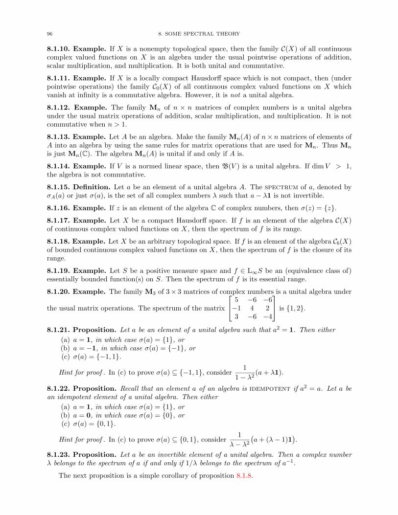
96 8. SOME SPECTRAL THEORY
8.1.10. Example. If X is a nonempty topological space, then the family C(X) of all continuouscomplex valued functions on X is an algebra under the usual pointwise operations of addition,scalar multiplication, and multiplication. It is both unital and commutative.
8.1.11. Example. If X is a locally compact Hausdorff space which is not compact, then (underpointwise operations) the family C0(X) of all continuous complex valued functions on X whichvanish at infinity is a commutative algebra. However, it is not a unital algebra.
8.1.12. Example. The family Mn of n × n matrices of complex numbers is a unital algebraunder the usual matrix operations of addition, scalar multiplication, and multiplication. It is notcommutative when n > 1.
8.1.13. Example. Let A be an algebra. Make the family Mn(A) of n× n matrices of elements ofA into an algebra by using the same rules for matrix operations that are used for Mn. Thus Mn
is just Mn(C). The algebra Mn(A) is unital if and only if A is.
8.1.14. Example. If V is a normed linear space, then B(V ) is a unital algebra. If dimV > 1,the algebra is not commutative.
8.1.15. Definition. Let a be an element of a unital algebra A. The spectrum of a, denoted byσA(a) or just σ(a), is the set of all complex numbers λ such that a− λ1 is not invertible.
8.1.16. Example. If z is an element of the algebra C of complex numbers, then σ(z) = z.
8.1.17. Example. Let X be a compact Hausdorff space. If f is an element of the algebra C(X)of continuous complex valued functions on X, then the spectrum of f is its range.
8.1.18. Example. Let X be an arbitrary topological space. If f is an element of the algebra Cb(X)of bounded continuous complex valued functions on X, then the spectrum of f is the closure of itsrange.
8.1.19. Example. Let S be a positive measure space and f ∈ L∞S be an (equivalence class of)essentially bounded function(s) on S. Then the spectrum of f is its essential range.
8.1.20. Example. The family M3 of 3× 3 matrices of complex numbers is a unital algebra under
the usual matrix operations. The spectrum of the matrix
5 −6 −6−1 4 23 −6 −4
is 1, 2.
8.1.21. Proposition. Let a be an element of a unital algebra such that a2 = 1. Then either
(a) a = 1, in which case σ(a) = 1, or(b) a = −1, in which case σ(a) = −1, or(c) σ(a) = −1, 1.
Hint for proof . In (c) to prove σ(a) ⊆ −1, 1, consider1
1− λ2(a+ λ1).
8.1.22. Proposition. Recall that an element a of an algebra is idempotent if a2 = a. Let a bean idempotent element of a unital algebra. Then either
(a) a = 1, in which case σ(a) = 1, or(b) a = 0, in which case σ(a) = 0, or(c) σ(a) = 0, 1.
Hint for proof . In (c) to prove σ(a) ⊆ 0, 1, consider1
λ− λ2
(a+ (λ− 1)1
).
8.1.23. Proposition. Let a be an invertible element of a unital algebra. Then a complex numberλ belongs to the spectrum of a if and only if 1/λ belongs to the spectrum of a−1.
The next proposition is a simple corollary of proposition 8.1.8.
8.1. THE SPECTRUM 97
8.1.24. Proposition. If a and b are elements of a unital algebra, then, except possibly for 0, thespectra of ab and ba are the same.
8.1.25. Definition. A map f : A→ B between Banach algebras is a (Banach algebra) homo-morphism if it is both an algebraic homomorphism and a continuous map between A and B. Wedenote by BALG the category of Banach algebras and continuous algebra homomorphisms.
8.1.26. Proposition. Let A and B be Banach algebras. The direct sum of A and B, denotedby A⊕B, is defined to be the set A×B equipped with pointwise operations:
(a) (a, b) + (a′, b′) = (a+ a′, b+ b′);(b) (a, b) (a′, b′) = (aa′, bb′);(c) α(a, b) = (αa, αb)
for a,a′ ∈ A, b, b′ ∈ B, and α ∈ C. As in 3.5.12 define ‖(a, b)‖ = ‖a‖ + ‖b‖. This makes A ⊕ Binto a Banach algebra.
8.1.27. Exercise. Identify products and coproducts (if they exist) in the category BALG ofBanach algebras and continuous algebra homomorphisms and in the category of Banach algebrasand contractive algebra homomorphisms. (Here contractive means ‖Tx‖ ≤ ‖x‖ for all x.)
8.1.28. Proposition. In a Banach algebra A the operations of addition and multiplication (re-garded as maps from A⊕A to A) are continuous and scalar multiplication (regarded as a map fromK⊕A to A) is also continuous.
8.1.29. Proposition (The Neumann series). Let a be an element of a unital Banach algebra. If‖a‖ < 1, then 1− a ∈ invA and (1− a)−1 =
∑∞k=0 a
k.
Hint for proof . Show that the sequence (1, a, a2, . . . ) is summable. (In a unital algebra we takea0 to mean 1.)
8.1.30. Corollary. If a is an element of a unital Banach algebra with ‖1 − a‖ < 1, then a isinvertible and
‖a−1‖ ≤ 1
1− ‖1− a‖.
8.1.31. Corollary. Suppose that a is an invertible element of a unital Banach algebra A, thatb ∈ A, and that ‖a− b‖ < ‖a−1‖−1. Then b is invertible in A.
Hint for proof . Use the preceding corollary to show that a−1b is invertible.
8.1.32. Corollary. If a belongs to a unital Banach algebra and ‖a‖ < 1, then
‖(1− a)−1 − 1‖ ≤ ‖a‖1− ‖a‖
.
8.1.33. Proposition. If A is a unital Banach algebra, then invA⊆ A.
Hint for proof . Let a ∈ invA. Show, for sufficiently small h, that 1− a−1h is invertible.
8.1.34. Proposition. Let A be a unital Banach algebra. The map a 7→ a−1 from invA into itselfis a homeomorphism.
8.1.35. Proposition. Let A be a unital Banach algebra. The map r : a 7→ a−1 from invA intoitself is differentiable and at each invertible element a, we have dra(h) = −a−1ha−1 for all h ∈ A.
Hint for proof . For a quick introduction to differentiation on infinite dimensional spaces, seeChapter 13 of my notes [16] on Real Analysis.
8.1.36. Proposition. Let a be an element of a unital Banach algebra A. Then the spectrum of ais compact and |λ| ≤ ‖a‖ for every λ ∈ σ(a).
98 8. SOME SPECTRAL THEORY
Hint for proof . Use the Heine-Borel theorem. To prove that the spectrum is closed notice that(σ(a))c = f←(invA) where f(λ) = a−λ1 for every complex number λ. Also show that if |λ| > ‖a‖,then 1− λ−1a is invertible.
8.1.37. Definition. Let a be an element of a unital Banach algebra. The resolvent mappingfor a is defined by
Ra : C \ σ(a)→ A : λ 7→ (a− λ1)−1 .
8.1.38. Definition. Let U⊆ C and A be a unital Banach algebra. A function f : U → A is
analytic on U if
f ′(a) := limz→a
f(z)− f(a)
z − aexists for every a ∈ U . A complex valued function which is analytic on all of C is an entirefunction.
8.1.39. Proposition. For a an element of a unital Banach algebra A and φ a bounded linearfunctional on A let f := φ Ra : C \ σ(a)→ C. Then
(a) f is analytic on its domain, and(b) f(λ)→ 0 as |λ| → ∞.
Hint for proof . For (i) notice that in a unital algebra a−1 − b−1 = a−1(b− a)b−1.
8.1.40. Theorem (Liouville). Every bounded entire function on C is constant.
Comment on proof . The proof of this theorem requires a little background in the theory ofanalytic functions, material that is not covered in these notes. The theorem would surely becovered in any first course in complex variables. For example, you can find a nice proof in [46],theorem 10.23.
8.1.41. Proposition. The spectrum of every element of a unital Banach algebra is nonempty.
Hint for proof . Argue by contradiction. Use Liouville’s theorem 8.1.40 to show that φ Ra isconstant for every bounded linear functional φ on A. Then use (a version of) the Hahn-Banachtheorem to prove that Ra is constant. Why must this constant be 0?
Note. It is important to keep in mind that we are working only with complex algebras. This result
is false for real Banach algebras. An easy counterexample is the matrix
[0 1−1 0
]regarded as an
element of the (real) Banach algebra M2 of all 2× 2 matrices of real numbers.
8.1.42. Theorem (Gelfand-Mazur). If A is a unital Banach algebra in which every nonzero ele-ment is invertible, then A is isometrically isomorphic to C.
Hint for proof . Let B = λ1 : λ ∈ C. Use the preceding proposition 8.1.41) to show thatB = A.
The following is an immediate consequence of the Gelfand-Mazur theorem 8.1.42 and proposi-tion 6.5.5.
8.1.43. Corollary. If I is a maximal ideal in a commutative unital Banach algebra A, then A/Iis isometrically isomorphic to C.
8.1.44. Proposition. Let a be an element of a unital algebra. Then
σ(an) = [σ(a)]n
for every n ∈ N. (The notation [σ(a)]n means λn : λ ∈ σ(a).)
8.1.45. Definition. Let a be an element of a unital algebra. The spectral radius of a, denotedby ρ(a), is defined to be sup|λ| : λ ∈ σ(a).
8.2. SPECTRA OF HILBERT SPACE OPERATORS 99
8.1.46. Proposition. If a is an element of a unital Banach algebra, then ρ(a) ≤ ‖a‖ and ρ(an) =(ρ(a)
)n.
8.1.47. Proposition. Let φ : A → B be a unital homomorphism between unital algebras. If a isan invertible element of A, then φ(a) is invertible in B and its inverse is φ(a−1).
8.1.48. Corollary. If φ : A→ B is a unital homomorphism between unital algebras, then
σ(φ(a)) ⊆ σ(a)
for every a ∈ A.
8.1.49. Corollary. If φ : A→ B is a unital homomorphism between unital algebras, then
ρ(φ(a)) ≤ ρ(a)
for every a ∈ A.
8.1.50. Theorem (Spectral radius formula). If a is an element of a unital Banach algebra, then
ρ(a) = inf‖an‖1/n : n ∈ N
= lim
n→∞‖an‖1/n .
8.1.51. Exercise. The Volterra operator V (defined in example 5.2.21) is an integral operator onthe Banach space C([0, 1]).
(a) Compute the spectrum of the operator V . (Hint. Show that ‖V n‖ ≤ (n!)−1 for everyn ∈ N and use the spectral radius formula.)
(b) What does (a) say about the possibility of finding a continuous function f which satisfiesthe integral equation
f(x)− µ∫ x
0f(t) dt = h(x),
where µ is a scalar and h is a given continuous function on [0, 1]?(c) Use the idea in (b) and the Neumann series expansion for 1− µV (see proposition 8.1.29)
to calculate explicitly (and in terms of elementary functions) a solution to the integralequation
f(x)− 12
∫ x
0f(t) dt = ex.
8.1.52. Proposition. Let A be a unital Banach algebra and B a closed subalgebra containing 1A.Then
(a) invB is both open and closed in B ∩ invA;(b) σA(b) ⊆ σB(b) for every b ∈ B; and(c) if b ∈ B and σA(b) has no holes (that is, if its complement in C is connected), then
σA(b) = σB(b).
Hint for proof . Consider the function fb : (σA(b))c → B ∩ invA : λ 7→ b− λ1.
8.2. Spectra of Hilbert Space Operators
8.2.1. Proposition. For a self-adjoint operator T on a Hilbert space the following are equivalent:
(i) σ(T ) ⊆ [0,∞);(ii) there exists an operator S on H such that T = S∗S; and
(iii) T is positive.
8.2.2. Notation. If A is a set of the complex numbers we define A∗ := λ : λ ∈ A. We do this toavoid confusion with the closure of the set A.
8.2.3. Proposition. If T is a Banach space operator then σ(T ∗) = σ(T ), while if it is a Hilbertspace operator then σ(T ∗) = (σ(T ))∗.
100 8. SOME SPECTRAL THEORY
In a finite dimensional space there is only one way that a complex number λ can end up inthe spectrum of an operator T . The reason for this is that there is only one way an operator, inthis case T − λI, on a finite dimensional space can fail to be invertible (see the paragraph beforedefinition 1.1.35). On the other hand there are several ways for λ to get into the spectrum of anoperator on an infinite dimensional space—because an operator has several ways in which it mayfail to be invertible. (See, for example, proposition 5.2.29.) Historically this has led to a numberof proposed taxonomies of the spectrum of an operator.
8.2.4. Definition. Let T be an operator on a Hilbert (or Banach) space H. A complex number λbelongs to the resolvent set of T if T − λI is invertible. The resolvent set is the complement ofthe spectrum of T . The set of complex numbers λ for which T −λI fails to be injective is the pointspectrum of T and is denoted by σp(T ). Members of the point spectrum of T are eigenvaluesof T . The set of complex numbers λ for which T − λI is not bounded away from zero is theapproximate point spectrum of T and is denoted by σap(T ). The set of all complex numbersλ such that the closure of the range of T − λI is a proper subspace of H is the compressionspectrum of T and is denoted by σc(T ). The residual spectrum of T , which we denote byσr(T ), is σc(T ) \ σp(T ).
8.2.5. Proposition. If T is a Hilbert space operator, then σp(T ) ⊆ σap(T ) ⊆ σ(T ).
8.2.6. Proposition. If T is a Hilbert space operator, then σ(T ) = σap(T ) ∪ σc(T ).
8.2.7. Proposition. If T is a Hilbert space operator, then σp(T∗) = (σc(T ))∗.
8.2.8. Corollary. If T is a Hilbert space operator, then σ(T ) = σap(T ) ∪ (σap(T∗))∗.
8.2.9. Theorem. Spectral Mapping Theorem If T is a Hilbert space operator and p is a polynomial,then
σ(p(T )) = p(σ(T )).
The preceding theorem is true more generally for any analytic function defined in a neighbor-hood of the spectrum of T . (For a proof see [8], chapter VII, theorem 4.10.) The result also holdsfor parts of the spectrum.
8.2.10. Proposition. If T is a Hilbert space operator and p is a polynomial, then
(a) σp(p(T )) = p(σp(T )),(b) σap(p(T )) = p(σap(T )), and(c) σc(p(T )) = p(σc(T )),
8.2.11. Proposition. If T is an invertible operator on a Hilbert space, then σ(T−1) = (σ(T ))−1.
8.2.12. Definition. As with vector spaces, two operators R and T on a Hilbert (or Banach) spaceH are similar if there exists an invertible operator S on H such that R = STS−1.
8.2.13. Proposition. If S and T are similar operators on a Hilbert space, then σ(S) = σ(T ),σp(S) = σp(T ), σap(S) = σap(T ), and σc(S) = σc(T ).
8.2.14. Proposition. If T is a normal operator on a Hilbert space, then σc(T ) = σp(T ), so thatσr(T ) = ∅.
8.2.15. Proposition. If T is an operator on a Hilbert space, then σap(T ) is closed.
8.2.16. Example. Let D = diag(a1, a2, a3, . . . ) be a diagonal operator on a Hilbert space and letA = ∪∞k=1ak. Then
(a) σp(D) = σc(D) = A,
(b) σap(D) = A, and(c) σr(D) = ∅.
8.2.17. Example. Let S be the unilateral shift operator on l2 (see example 5.2.11). Then
8.2. SPECTRA OF HILBERT SPACE OPERATORS 101
(a) σ(S) = D,(b) σp(S) = ∅,(c) σap(S) = C,(d) σc(S) = B,(e) σ(S∗) = D,(f) σp(S
∗) = B,(g) σap(S
∗) = D, and(h) σc(S
∗) = ∅.where B is the open unit disk, D is the closed unit disk, and C is the unit circle in the complexplane.
8.2.18. Example. Let (S,A, µ) be a σ-finite positive measure space, φ ∈ L∞(S, µ), and Mφ bethe corresponding multiplication operator on the Hilbert space L2S, µ (see example 5.2.15). Thenthe spectrum and the approximate point spectrum of Mφ are the essential range of φ, while thepoint spectrum and compression spectrum of Mφ are λ ∈ C : µ(φ←(λ)) > 0.

CHAPTER 9
TOPOLOGICAL VECTOR SPACES
9.1. Balanced Sets and Absorbing Sets
9.1.1. Definition. A set S in a vector space is balanced (or circled) if DS ⊆ S.
9.1.2. Notation. Let D denote the closed unit disk in the complex plane z ∈ C : |z| ≤ 1.
9.1.3. Proposition. Let B be a balanced subset of a vector space. If α and β are scalars such that|α| ≤ |β|, then αB ⊆ βB.
9.1.4. Corollary. If B is a balanced subset of a vector space and |λ| = 1, then λB = B.
9.1.5. Definition. If S is a subset of a vector space, then the set DS is the balanced hull of S.
9.1.6. Proposition. Let S be a subset of a vector space V . Then the balanced hull of S is theintersection of all the balanced subsets of V which contain S; thus it is the smallest balanced subsetof V containing S.
9.1.7. Definition. A subset A of a vector space V absorbs a subset B ⊆ V if there exists M > 0such that B ⊆ tA whenever |t| ≥ M . The set A is absorbing (or radial) if it absorbs everyone-element set (equivalently, every finite set).
Thus, speaking loosely, a set is absorbing if any vector in the space can be covered by anappropriate dilation of the set.
9.1.8. Example. Let B be the union of the x- and y-axes in the real vector space R2. Then B isbalanced but not convex.
9.1.9. Example. In the vector space C an ellipse with one focus at the origin is an example of anabsorbing set which is not balanced.
9.1.10. Example. In the vector space C2 the set D× 0 is balanced but not absorbing.
9.1.11. Proposition. A balanced set B in a vector space V is absorbing if and only if for everyx ∈ V there exists a scalar α 6= 0 such that αx ∈ B.
9.2. Filters
In the study of topological vector spaces it is convenient to use the language of filters tocharacterize topological properties of the spaces. It is a tool, alternative, but largely equivalent, tonets, useful especially in (nonmetric) situations where sequences are no longer helpful.
Roughly, a filter is a nonempty family of nonempty sets which is closed under finite intersectionsand supersets.
9.2.1. Definition. A nonempty family F of nonempty subsets of a set S is a filter on S if
(a) A, B ∈ F implies A ∩B ∈ F, and(b) if A ∈ F and A ⊆ B, then B ∈ F.
9.2.2. Example. A simple (and, for our work, the most important) example of a filter is the familyof neighborhoods of a point a in a topological space. This is the neighborhood filter at a. Itwill be denoted by Na.
103
104 9. TOPOLOGICAL VECTOR SPACES
9.2.3. Definition. A nonempty family B of nonempty sets of a set S is a filterbase on S if forevery A, B ∈ B there exists C ∈ B such that C ⊆ A ∩B.
We say that a subfamily B of a filter F is a filterbase for F if every member of F containsa member of B. (It is important to check that any such subfamily really is a filterbase.)
9.2.4. Example. Every filter is a filterbase.
9.2.5. Example. Let a be a point in a topological space. Any neighborhood base at a is a filterbasefor the filter Na of all neighborhoods of a. In particular, the family of all open neighborhoods of ais a filterbase for Na.
9.2.6. Example. Let B be a filterbase in a set S. Then the family F of all supersets of membersof B is a filter in S and B is a filterbase for F. We will call this filter the filter generatedby B.
9.2.7. Definition. A filterbase (in particular, a filter) B on a topological space X converges toa point a ∈ X if every member N of Na, the neighborhood filterbase at a, contains a member of B.In this case we write B→ a.
9.2.8. Proposition. A filterbase on a Hausdorff topological space converges to at most one point.
9.2.9. Example. Let (xλ) be a net in a set S and F be the family of all A ⊆ S for which thenet (xλ) is eventually in A. Then F is a filter in S. We will call this the filter generated by thenet (xλ).
9.2.10. Proposition. Suppose that (xλ) is a net in a topological space X, that F is the filtergenerated by (xλ), and a ∈ X. Then F→ a if and only if xλ → a.
9.2.11. Example. Let B be a filter base on a set S. Let D be the set of all ordered pairs (b, B)such that b ∈ B ∈ B. For (b1, B1), (b2, B2) ∈ D define (b1, B1) ≤ (b2, B2) if B2 ⊆ B1. This makesD into a directed set. Now create a net in S by defining
x : D → S : (b, B) 7→ b
that is, let xλ = b for all λ = (b, B) ∈ D. Then(xλ)λ∈D is a net in S. It is the net generated by
(or based on) the filter base B.
9.2.12. Proposition. Let B be a filter base in a topological space X, let (xλ) the the net generatedby B, and let a ∈ X. Then xλ → a if and only if B→ a.
9.3. Compatible Topologies
9.3.1. Definition. Let T be a topology on a vector space X. We say that T is compatible withthe linear structure on X if the operations of addition A : X ×X → X : (x, y) 7→ x+ y and scalarmultiplication M : K×X : (α, x) 7→ αx are continuous. (Here we understand X ×X and K×X tobe equipped with the product topology.)
If X is a vector space on which has been defined a topology T compatible with its linearstructure, we say that the pair (X,T) is a topological vector space. (As you doubtlessexpect, we will almost always continue using standard illogical abridgements such as “Let X be atopological vector space . . . ”.) We denote by TVS the category of topological vector space andcontinuous linear maps.
9.3.2. Example. Let X be a nonzero vector space. The discrete topology on X is not compatiblewith the linear structure on X.
9.3.3. Proposition. Let X be a topological vector space, a ∈ X, and α ∈ K.
(a) The mapping Ta : x 7→ x+ a ( translation by a) of X into itself is a homeomorphism.(b) If α 6= 0, the mapping x 7→ αx of X into itself is a homeomorphism.
9.3. COMPATIBLE TOPOLOGIES 105
9.3.4. Corollary. A set U is a neighborhood of a point x in a topological vector space if and onlyif −x+ U is a neighborhood of 0.
9.3.5. Corollary. Let U be a filterbase for the neighborhood filter at the origin in a topologicalvector space X. A subset V of X is open if and only if for every x ∈ V there exists U ∈ U suchthat x+ U ⊆ V .
What the preceding corollary tells us is that the topology of a topological vector space iscompletely determined by a filterbase for the neighborhood filter at the origin of the space. Wecall such a filterbase a local base (for the topology).
9.3.6. Proposition. If U is a neighborhood of the origin in a topological vector space and 0 6= λ ∈K, then λU is a neighborhood of the origin.
9.3.7. Proposition. In a topological vector space every neighborhood of 0 contains a balancedneighborhood of 0.
9.3.8. Proposition. In a topological vector space every neighborhood of 0 every neighborhood ofthe origin is absorbing.
9.3.9. Proposition. If V is a neighborhood of 0 in a topological vector space, then there exists aneighborhood U of 0 such that U + U ⊆ V .
The next proposition is (almost) a converse of the preceding three.
9.3.10. Proposition. Let X be a vector space and U be a filterbase on X which satisfies thefollowing conditions:
(a) every member of U is balanced;(b) every member of U is absorbing; and(c) for every V ∈ U there exists U ∈ U such that U + U ⊆ V .
Then there exists a topology T on X under which X is a topological vector space and U is a localbase for T.
9.3.11. Example. In a normed linear space the family Cr(0) : r > 0 of closed balls about theorigin is a local base for the topology on the space.
9.3.12. Example. Let Ω be a nonempty open subset of Rn. For every compact subset K ⊆ Ω andevery ε > 0 let UK,ε = f ∈ C(Ω): |f(x)| ≤ ε whenever x ∈ K. Then the family of all such setsUK,ε is a local base for a topology on C(Ω). This is the topology of uniform convergenceon compact sets.
9.3.13. Proposition. Let A be a subset of a topological vector space and 0 6= α ∈ K. ThenαA = αA.
9.3.14. Proposition. Let S be a set in a topological vector space.
(a) If S is balanced, so is its closure.(b) The balanced hull of S may fail to be closed even if S itself is closed.
Hint for proof . For (b) let S be the hyperbola in R2 whose equation is xy = 1.
9.3.15. Proposition. If M is a vector subspace of a topological vector space, then so is M .
It is clear that every absorbing set in a topological vector space must contain the origin. Thenext example shows, however, that it need not contain a neighborhood of the origin.
9.3.16. Example (Schatz’s apple). In the real vector space R2 the set
C1
((−1, 0)
)∪ C1
((1, 0)
)∪(0 × [−1, 1]
)is absorbing, but is not a neighborhood of the origin.
106 9. TOPOLOGICAL VECTOR SPACES
The next result tells us that in a topological vector space compact sets and closed sets can beseparated by open sets if they are disjoint.
9.3.17. Proposition. If K and C are nonempty disjoint subsets of a topological space X with Kcompact and C closed, then there is a neighborhood V of the origin such that (K+V )∩(C+V ) = ∅.
9.3.18. Corollary. If K is a compact subset of a Hausdorff topological vector space X and C is aclosed subset of X, then K + C is closed in X.
Hint for proof . Let x ∈ (K + C)c. Consider the sets x−K and C.
9.3.19. Corollary. Every member of a local base B for a topological vector space contains theclosure of a member of B.
9.3.20. Proposition. Let X be a topological vector space. Then the following are equivalent.
(a) 0 is a closed set in X.(b) x is a closed set for every x ∈ X.(c) For every x 6= 0 in X there exists a neighborhood of the origin to which x does not belong.(d)
⋂U = 0 where U is a local base for X.
(e) X is Hausdorff
9.3.21. Definition. A topological space is regular if points and closed sets can be separated byopen sets; that is, if C is a closed subset of the space and x is a point of the space not in C, thenthere exist disjoint open sets U and V such that C ⊆ U and x ∈ V .
9.3.22. Proposition. Every Hausdorff topological vector space is regular.
9.3.23. Corollary. If X is a topological space in which points are closed sets, then X is regular.
9.3.24. Proposition. Let X be a Hausdorff topological vector space. If M is a subspace of X andF is a finite dimensional vector subspace of X, then M + F is closed in X. (In particular, F isclosed.)
9.3.25. Definition. A subset B of a topological vector space is bounded if for every neighborhoodU of 0 in the space there exists α > 0 such that B ⊆ αU .
9.3.26. Proposition. A subset of a topological vector space is bounded if and only if it is absorbedby every neighborhood of 0.
9.3.27. Proposition. A subset B of a topological vector space is bounded if and only if αnxn → 0whenever (xn) is a sequence of vectors in B and (αn) is a sequence of scalars in c0.
9.3.28. Proposition. If a subset of a topological vector space is bounded, then so is its closure.
9.3.29. Proposition. If subsets A and B of a topological vector space are bounded, then so isA ∪B.
9.3.30. Proposition. If subsets A and B of a topological vector space are bounded, then so isA+B.
9.3.31. Proposition. Every compact subset of a topological vector space is bounded.
As is the case with normed linear spaces, we say that linear maps are bounded if they takebounded sets to bounded sets.
9.3.32. Definition. A linear map T : X → Y between topological vector spaces is bounded ifT→(B) is a bounded subset of Y whenever B is a bounded subset of X.
9.3.33. Proposition. Every continuous linear map between topological vector spaces is bounded.
9.4. QUOTIENTS 107
9.3.34. Definition. A filter F on a subset A of a topological vector space X is a Cauchy filterif for every neighborhood U of the origin in X there exists B ⊆ A such that
B −B ⊆ U .
9.3.35. Proposition. On a topological vector space every convergent filter is Cauchy.
9.3.36. Definition. A subset A of a topological vector space X is complete if every Cauchy filteron A converges to a point of A.
9.3.37. Proposition. Every complete subset of a Hausdorff topological vector space is closed.
9.3.38. Proposition. If C is a closed subset of a complete set in a topological vector space, thenC is complete.
9.3.39. Proposition. A linear map T : X → Y between topological vector spaces, is continuous ifand only if it is continuous at zero.
9.4. Quotients
9.4.1. Convention. As is the case with Hilbert and Banach spaces the word “subspace” in thecontext of topological vector spaces means closed vector subspace.
9.4.2. Definition. Let M be a vector subspace of a topological vector space X and π : X →X/M : x 7→ [x] be the usual quotient map. On the quotient vector space X/M we define a topology,which we call the quotient topology, by specifying the neighborhood filter at the origin in X/Mto be the image under π of the neighborhood filter at the origin in X. That is, we declare a subsetV of X/M to be a neighborhood of 0 when, and only when, there exists a neighborhood U of theorigin in X such that V = π→(U).
9.4.3. Proposition. Let M be a vector subspace of a topological vector space X. When X/M isgiven the quotient topology the quotient map π : X → X/M is both an open map and continuous.
9.4.4. Example. Let M be the y-axis in the topological vector space R2 (with its usual topology).Identify R2/M with the x-axis. Although the quotient map takes open sets to open sets, thehyperbola (x, y) ∈ R2 : xy = 1 shows that π need not take closed sets to closed sets.
9.4.5. Proposition. Let M be a vector subspace of a topological vector space X. The quotienttopology on X/M is the largest topology under which the quotient map is continuous.
The next proposition assures us that the quotient topology, as defined above, makes the quotientvector space into a topological vector space.
9.4.6. Proposition. Let M be a vector subspace of a topological vector space X. The quotienttopology on X/M is compatible with the vector space operations on that space.
9.4.7. Proposition. If M is a vector subspace of a topological vector space X, then the quotientspace X/M is a Hausdorff if and only if M is closed in X.
9.4.8. Exercise. Explain also how the preceding proposition enables us to associate with a non-Hausdorff topological vector space another space that is Hausdorff.
9.4.9. Proposition. Let T : X → Y be a linear map between topological vector spaces and M be a
subspace of X. If M ⊆ kerT , then there exists a unique function T : X/M → Y such that T = T π(where π is the quotient map). The function T is linear; it is continuous if and only if T is; it isopen if and only if T is.
108 9. TOPOLOGICAL VECTOR SPACES
9.5. Locally Convex Spaces and Seminorms
9.5.1. Proposition. In a topological vector space the closure of a convex set is convex.
9.5.2. Proposition. In a topological vector space every convex neighborhood of 0 contains a bal-anced convex neighborhood of 0.
9.5.3. Proposition. A closed subset C of a topological vector space is convex if and only if 12(x+y)
belongs to C whenever x and y do.
9.5.4. Proposition. If a subset of a topological vector space is convex so are its closure and itsinterior.
9.5.5. Definition. A topological vector space is locally convex if it has a local base consistingof convex sets. For brevity we will refer to a locally convex topological vector space simply as alocally convex space.
9.5.6. Proposition. If p is a seminorm on a vector space, then p(0) = 0.
9.5.7. Proposition. If p is a seminorm on a vector space V , then |p(x)− p(y)| ≤ p(x− y) for allx, y ∈ V .
9.5.8. Corollary. If p is a seminorm on a vector space V , then p(x) ≥ 0 for all x ∈ V .
9.5.9. Proposition. If p is a seminorm on a vector space V , then p←(0) is a vector subspaceof V .
9.5.10. Definition. Let p be a seminorm on a vector space V and ε > 0. We will call the setBp,ε := p←
([0, ε)
)the open semiball of radius ε at the origin determined by p. Similarly, the set
Cp,ε := p←([0, ε]
)is the closed semiball of radius ε at the origin determined by p. For the open
and closed semiballs of radius one determined by p use the notations Bp and Cp, respectively.
9.5.11. Proposition. Let P be a family of seminorms on a vector space V . The family U ofall finite intersections of open semiballs at the origin of V induces a (not necessarily Hausdorff)topology on V which is compatible with the linear structure of V and for which U is a local base.
Hint for proof . Proposition 9.3.10.
9.5.12. Proposition. Let p be a seminorm on a topological vector space X. Then the followingare equivalent:
(a) Bp is open in X;(b) p is continuous at the origin; and(c) p is continuous.
9.5.13. Proposition. If p and q are continuous seminorms on a topological vector space, then soare p+ q and maxp, q.9.5.14. Example. Let N be an absorbing, balanced, convex subset of a vector space V . Define
µN
: V → R : x 7→ infλ > 0: x ∈ λN.The function µ
Nis a seminorm on V . It is called the Minkowski functional of N .
9.5.15. Proposition. If N is an absorbing balanced convex set in a vector space V and µN
is theMinkowski functional of N , then
BµN⊆ N ⊆ Cµ
N
and the Minkowski functionals generated by the three sets BµN
, N , and CµN
are all identical.
9.5.16. Proposition. If N is an absorbing balanced convex set in a vector space V and µN
is theMinkowski functional of N , then µ
Nis continuous if and only if N is a neighborhood of zero, in
which caseBµ
N= N and Cµ
N= N.
9.6. FRECHET SPACES 109
9.5.17. Corollary. Let N be an absorbing, balanced, convex, closed subset of a topological vectorspace X. Then the Minkowski functional µ
Nis the unique seminorm on X such that N = Cµ
N.
9.5.18. Proposition. Let p be a seminorm on a vector space V . Then the set Bp is absorbing,balanced, and convex. Furthermore, p = µ
Bp.
9.5.19. Definition. A family P of seminorms on a vector space V is separating if for everyx ∈ X there exists p ∈ P such that p(x) 6= 0.
9.5.20. Proposition. In a topological vector space let B be a local base consisting of balancedconvex open sets. Then µ
N: N ∈ B is a separating family of continuous seminorms on the space
such that N = BµN
for every N ∈ B.
The next proposition demonstrates the way in which many of the most important locally convexspaces arise—from a separating family of seminorms.
9.5.21. Proposition. Let P be a separating family of seminorms on a vector space V . For eachp ∈ P and each n ∈ N let Up,n = p←
([0, 1
n)). Then the family of all finite intersections of the sets
Up,n comprises a balanced convex local base for a topology on V under which V becomes a locallyconvex space and every seminorm in P is continuous.
9.5.22. Example. Let X be a locally compact Hausdorff space. For every nonempty compactsubset K of X define
pK
: C(X)→ K : f 7→ sup|f(x)| : x ∈ K.Then the family P of all p
Kwhere K is a nonempty compact subset of X is a family of seminorms
under which C(X) becomes a locally convex space.
9.5.23. Proposition. A linear map T : V →W from a topological vector space to a locally convexspaces is continuous if and only if p T is a continuous seminorm on V for every continuousseminorm p on W .
9.5.24. Proposition. Let p be a continuous seminorm on a subspace M of a locally convex space X.Then p can be extended to a continuous linear functional on all of X.
Proof. See [8], proposition IV.5.13.
9.6. Frechet Spaces
9.6.1. Definition. A topological space (X,T) is metrizable if there exists a metric d on X ×Xsuch that the topology generated by d is T.
9.6.2. Definition. A metric d on a vector space V is translation invariant if
d(x, y) = d(x+ a, y + a)
for all x, y, and a in V .
9.6.3. Proposition. Let (X,T) be a Hausdorff topological vector space with a countable local base.Then there exists a translation invariant metric d on V which generates the topology T and whoseopen balls at the origin are balanced. If X is a locally convex space then d may be chosen so that,additionally, its open balls are convex.
Proof. See [47], theorem 1.24.
9.6.4. Example. Let pn : n ∈ N be a a countable separating family of seminorms on a vectorspace X and T be the topology on X guaranteed by proposition 9.5.21. In this case we can explicitlydefine a translation invariant metric on X which induces the topology T. For an arbitrary sequence(αk)∈ c0 a metric with the desired properties is given by
d(x, y) = maxk∈N
αkpk(x− y)
1 + pk(x− y)
.
110 9. TOPOLOGICAL VECTOR SPACES
Proof. See [47], remark 1.38(c).
9.6.5. Definition. A Frechet space is a complete metrizable locally convex space.
9.6.6. Notation. Let A and B be subsets of a topological space. We write A ≺ B if A ⊆ B.
9.6.7. Proposition. The following hold for subsets A, B, and C of a topological space:
(a) if A ≺ B and B ≺ C, then A ≺ C;(b) if A ≺ C and B ≺ C, then A ∪B ≺ C; and(c) if A ≺ B and A ≺ C, then A ≺ B ∩ C.
Here is a standard result from elementary topology.
9.6.8. Proposition. Let Ω be a nonempty open subset of Rn. The there exists a sequence (Kn) of
nonempty compact subsets of Ω such that Ki ≺ Kj whenever i < j and∞⋃i=1
Ki = Ω.
Proof. See [49], lemma 10.1.
9.6.9. Example. Let Ω be a nonempty open subset of some Euclidean space Rn and C(Ω) bethe family of all continuous scalar valued functions on Ω. By the preceding proposition we canwrite Ω as the union of a countable collection of nonempty compact sets K1, K2, . . . such thatKi ≺ Kj whenever i < j. For each n ∈ N and f ∈ C(Ω) let pn(f) = sup|f(x)| : x ∈ Kn as inexample 9.5.22. According to proposition 9.5.21 this family of seminorms makes C(Ω) into a locallyconvex space. Let T be the resulting topology on this space. By example 9.6.4 the function
d(f, g) = maxk∈N
2−kpk(f − g)
1 + pk(f − g)
defines a metric on C(Ω) which induces the topology T. Under this metric C(Ω) is a Frechet space.
9.6.10. Notation (Multi-index notation). Let Ω be an open subset of a Euclidean space Rn. Wewill consider infinitely differentiable scalar valued functions on Ω; that is, functions on Ω which havederivatives of all orders at each point of Ω. We will refer to such functions as smooth functionson Ω. The class of all smooth functions on Ω is denoted by C∞(Ω).
Another important class we will consider is C∞c (Ω), the family of all infinitely differentiablescalar valued functions on Ω which have compact support; that is, which vanish outside of somecompact subset of Ω. The functions in this family are frequently called test functions on Ω.Another, shorter, notation in common use for this family is D(Ω).
We will be interested in differential operators on the spaces D(Ω). Let α = (α1, . . . , αn) be amulti-index, that is, an n-tuple of integers where each αk ≥ 0, and let
Dα =
(∂
∂x1
)α1
. . .
(∂
∂xn
)αn.
The order of the differential operator Dα is |α| :=∑n
k=1 αk. (When |α| = 0 we understand
Dα(f) = f for each function f .) An alternative notation for Dαf is f (α).
9.6.11. Example. On the family C∞(Ω) of smooth functions on a open subset Ω of a Euclideanspace Rn define a family p
K,j of seminorms. For each compact subset K of Ω and each j ∈ N let
pK,j
(f) = sup|Dαf(x)| : x ∈ K and |α| ≤ j.
This family of seminorms makes C∞(Ω) into a Frechet space. The resulting topology on C∞(Ω) issometimes called the topology of uniform convergence on compacta of the functions and all theirderivatives.
Hint for proof . To see that the space is metrizable use example 9.6.4 and proposition 9.6.8.
9.6. FRECHET SPACES 111
9.6.12. Example. Let n ∈ N . Denote by S = S(Rn) the space of all smooth functions f definedon all of Rn which satisfy
lim‖x‖→∞
‖x‖k|Dαf(x)| = 0
for all multi-indices α = (α1. . . . , αn) ∈ Nn and all integers k ≥ 0. Such functions are frequentlyreferred to as functions with rapidly decreasing derivatives or even more simply as rapidly decreasingfunctions. On S we place the topology defined by the seminorms
pm,k
:= sup|α|≤m
supx∈Rn(1 + ‖x‖2)m|(Dαf)(x)|
for k, m = 0, 1, 2, . . . . The resulting space is a Frechet space called the Schwartz space of Rn.
Hint for proof . For a proof of completeness see [49], Example IV, pages 92–94.
9.6.13. Proposition. A test function ψ on R is the derivative of another test function if and onlyif∫∞−∞ ψ = 0.
9.6.14. Proposition. Let F be a Frechet space whose topology is induced by a translation invariantmetric. Then every bounded subset of F a has finite diameter.
9.6.15. Example. Consider the Frechet space R with the topology induced by the translation
invariant metric d(x, y) =|x− y|
1 + |x− y|. Then the set N of natural numbers has finite diameter but
is not bounded.

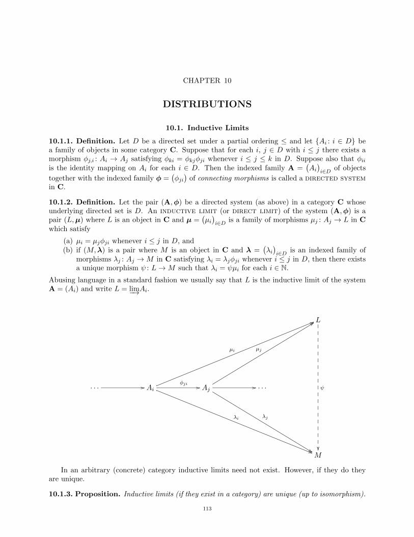
CHAPTER 10
DISTRIBUTIONS
10.1. Inductive Limits
10.1.1. Definition. Let D be a directed set under a partial ordering ≤ and let Ai : i ∈ D bea family of objects in some category C. Suppose that for each i, j ∈ D with i ≤ j there exists amorphism φj,i : Ai → Aj satisfying φki = φkjφji whenever i ≤ j ≤ k in D. Suppose also that φiiis the identity mapping on Ai for each i ∈ D. Then the indexed family A =
(Ai)i∈D of objects
together with the indexed family φ =(φji)
of connecting morphisms is called a directed systemin C.
10.1.2. Definition. Let the pair (A,φ) be a directed system (as above) in a category C whoseunderlying directed set is D. An inductive limit (or direct limit) of the system (A,φ) is apair (L,µ) where L is an object in C and µ =
(µi)i∈D is a family of morphisms µj : Aj → L in C
which satisfy
(a) µi = µjφji whenever i ≤ j in D, and(b) if (M,λ) is a pair where M is an object in C and λ =
(λi)i∈D is an indexed family of
morphisms λj : Aj →M in C satisfying λi = λjφji whenever i ≤ j in D, then there existsa unique morphism ψ : L→M such that λi = ψµi for each i ∈ N.
Abusing language in a standard fashion we usually say that L is the inductive limit of the systemA = (Ai) and write L = lim−→Ai.
L
ψ
· · · // Ai
µi
55
λi
))
φji // Aj
µj
99
λj
%%
// · · ·
M
In an arbitrary (concrete) category inductive limits need not exist. However, if they do theyare unique.
10.1.3. Proposition. Inductive limits (if they exist in a category) are unique (up to isomorphism).
113
114 10. DISTRIBUTIONS
10.1.4. Example. Let S be a nonempty object in the category SET. Consider the family P(S)of all subsets of S directed by the partial ordering ⊆. Whenever A ⊆ B ⊆ S, take the connectingmorphism ι
BAto be the inclusion mapping from A into B. Then P(S), together with the family
of connecting morphisms, form a directed system. The inductive limit if this system is S.
10.1.5. Example. Direct limits exist in the category VEC of vector spaces and linear maps.
Hint for proof . Let (V,φ) be a directed system in VEC (as in definition 10.1.1) and D be
its underlying directed set. For the inductive limit of this system try∏i∈D
Vi
/⊕i∈D
Vi (see exam-ples 3.5.10 and 3.6.10).
It is helpful to keep in mind that two elements x and y in the quotient space lie in the sameequivalence class if their difference has finite support, that is, if xi and yi are eventually equal.You may find it helpful to make use of the functions νi : Vi →
∏k∈D
Vk (where i ∈ D) defined by
νi(u) =
φji(u), if i ≤ j ;0, otherwise.
10.1.6. Example. The sequence Z 1 // Z 2 // Z 3 // Z 4 // . . . (where n : Z → Z satisfiesn(1) = n) is an inductive sequence of Abelian groups whose inductive limit is the set Q of rationalnumbers.
10.1.7. Example. The sequence Z 2 // Z 2 // Z 2 // Z 2 // . . . is an inductive sequence ofAbelian groups whose inductive limit is the set of dyadic rational numbers.
10.2. LF -spaces
Since our principal goal in this chapter is an introduction to the theory of distributions, wewill from now on restrict our attention to an especially simple type of inductive limit—the strictinductive limit of an inductive sequence. In particular, we will interested in strict inductive limitsof increasing sequences of Frechet spaces.
Recall that a weak topology on a set S is induced by a family of functions fα : S → Xα mappinginto topological spaces. It is the weakest topology on S which makes all these functions continuous(see exercise 4.6.2). A dual notion is that of a strong topology, a topology induced by a familyof functions mapping from topological spaces Xα into S. It is the strongest topology under whichall these functions are continuous. One strong topology which we have already encountered is thequotient topology (see proposition 9.4.5). Another important example, which we introduce next, isthe inductive limit topology.
10.2.1. Definition. A strict inductive sequence is a sequence (Xi) of locally convex spacessuch that for each i ∈ N
(i) Xi is a closed subspace of Xi+1 and(ii) the topology Ti on the space Xi is the restriction to Xi of the sets belonging to Ti+1.
This is, of course, a directed system in which the connecting morphisms φji are just the inclusionmaps of Xi into Xj for i < j.
The strict inductive limit of such a sequence of spaces is their union L =⋃∞i=1Xi. We
give L the largest locally convex topology under which all the inclusion maps ψi : Xi → L arecontinuous. This is the inductive limit topology on L.
10.2.2. Proposition. The inductive limit topology defined above exists.
10.2.3. Definition. The strict inductive limit of a sequence of Frechet spaces is an LF -space.
10.2.4. Example. The space D(Ω) = C∞c (Ω) of test functions on an open subset Ω of a Euclideanspace is an LF -space (see notation 9.6.10).
10.2.5. Proposition. Every LF -space is complete.
10.3. DISTRIBUTIONS 115
Proof. See [49], theorem 13.1.
10.2.6. Proposition. Let T : L→ Y be a linear map from an LF -space to a locally convex space.Suppose that L = lim−→Xk where (Xk) is a strict inductive sequence of Frechet spaces. Then T is
continuous if and only if its restriction T∣∣Xk
to each Xk is continuous.
Proof. See [49], proposition 13.1, or [8], proposition IV.5.7, or [21], theorem B.18(c).
CAUTION. Francois Treves, in his beautifully written book on Topological Vector Spaces, Dis-tributions, and Kernels, warns his readers against a particularly insidious error: it is very easy toassume that if M is a closed vector subspace of an LF -space L = lim−→Xk, then the topology which
M inherits from L must be the same as the inductive limit topology it gets from the strict inductivesequence of Frechet spaces M ∩Xk. This turns out not to be true in general.
10.2.7. Proposition. Let T : L→ Y be a linear map from an LF -space to a locally convex space.Then T is continuous if and only if it is sequentially continuous.
10.3. Distributions
10.3.1. Definition. Let Ω be a nonempty open subset of Rn. A function f : Ω → R is locallyintegrable if
∫K |f | dµ <∞ for every compact subset K of Ω. (Here µ is the usual n-dimensional
Lebesgue measure.) The family of all such functions on Ω is denoted by Lloc1 (Ω).
10.3.2. Example. The constant function 1 on the real line is locally integrable, even though it iscertainly not integrable.
A locally integrable function need not even be continuous. On the real line, for example, thecharacteristic function of any Lebesgue measurable set is locally integrable. Imagine how convenientit would be if we could speak meaningfully of the derivative of any such function and, even better,be permitted to differentiate it as often as we please. — Welcome to the world of distributions.Here
(a) every locally integrable function may be regarded as a distribution, and(b) every distribution is infinitely differentiable, and furthermore,(c) all the familiar differentiation rules of beginning calculus hold.
10.3.3. Definition. Let Ω be a nonempty open subset of Rn. A distribution is a continuouslinear functional on the space D(Ω) = C∞c (Ω) of test functions on Ω. Although such a functionalis, technically, defined on a space of functions on Ω, we will follow the usual sloppy practice andrefer to it as a distribution on Ω. The set of all distributions on Ω, the dual space of D(Ω) will bedenoted by D∗(Ω).
10.3.4. Proposition. Let Ω be an open subset of Rn. A linear functional L on the space D(Ω)of test functions on Ω is a distribution if and only if L(φk) → 0 whenever (φk) is a sequence of
test functions such that φ(α)k → 0 uniformly for every multi-index α and there exists a compact set
K ⊆ Ω which contains the support of each φk.
Proof. See [8], proposition IV.5.21 or [49], proposition 21.1(b).
10.3.5. Example. If Ω is a nonempty open subset of Rn and f is a locally integrable function onΩ, then the map
Lf : D(Ω)→ K : φ 7→∫fφ dλ
is a distribution. Such a distribution is called a regular distribution. A distribution which is notregular is called a singular distribution.
116 10. DISTRIBUTIONS
Note. Let u be a distribution and φ be a test function on Ω. Standard notations for u(φ) are
〈u, φ〉 and 〈φ, u〉. Also we use the notation f for Lf . Thus in the preceding example
〈f , φ〉 = 〈φ, f〉 = f(φ) = 〈Lf , φ〉 = 〈φ,Lf 〉 = Lf (φ)
for f ∈ Lloc1 (Ω).
10.3.6. Example. If µ is a regular Borel measure on a nonempty open subset Ω of Rn and f is alocally integrable function on Ω, then the map
Lµ : D(Ω)→ R : φ 7→∫
Ωfφ dµ
is a distribution on Ω.
10.3.7. Notation. Let a ∈ R. Define µa, Dirac measure concentrated at a, on the Borel sets ofR by
µa(B) =
1, if a ∈ B0, if a /∈ B.
We denote the corresponding distribution by δa and call it the Dirac delta distribution at a.Thus δa = Lµa . If a = 0, we write δ for δ0. Historically the distribution δ has been afflicted with anotoriously misleading (although not technically incorrect) name: the Dirac delta function.
10.3.8. Example. If δa is the Dirac delta distribution at a point a ∈ R and φ is a test functionon R, then δa(φ) = φ(a).
10.3.9. Notation. Let H denote the characteristic function of the interval [0,∞). This is the
Heaviside function. Its corresponding distribution H = LH is the Heaviside distribution.
10.3.10. Example. If H is the Heaviside distribution and φ ∈ D(R), then H(φ) =∫∞
0 φ.
10.3.11. Example. Let f be a differentiable function on R whose derivative is locally integrable.Then
Lf ′(φ) = −Lf (φ ′) (10.3.1)
for every φ ∈ D(R).
Hint for proof . Integration by parts.
Now an important question arises: How can we define the “derivative” of a distribution? It iscertainly natural to want a regular distribution to behave in much the same way as the functionfrom which it arises. That is, we would like the derivative (Lf )′ of a regular distribution Lf tocorrespond with the regular distribution arising from the derivative of the function f . That is tosay, what we want is (Lf )′ = Lf ′ . This suggests, according to the preceding example, that fordifferentiable functions f with locally integrable derivatives we should define
(Lf )′(φ) = −Lf (φ ′) (10.3.2)
for every φ ∈ D(R). The observation that the right side of the equation (10.3.2) makes sense forany distribution whatever motivates the following definition.
10.3.12. Definition. Let u be a distribution on a nonempty open subset Ω of R. We define u ′,the derivative of u, by
u ′(φ) := −u(φ ′)
for every test function φ on Ω. We also use the notation Du for the derivative of u.
10.3.13. Example. The Dirac distribution δ is the derivative of the Heaviside distribution H.
10.3.14. Exercise. Let S be the signum (or sign) function on R; that is, let S = 2H − 1, whereH is the Heaviside function. Also let g be the function on R such that g : x 7→ −x − 3 for x < 0and g : x 7→ x+ 5 for x ≥ 0.
10.3. DISTRIBUTIONS 117
(a) Find constants α and β such that g′ = αS + βδ.
(b) Find a function a on R such that a′ = S.
10.3.15. Exercise. Let f(x) =
1− |x|, if |x| ≤ 1;0, otherwise.
By calculating both sides of equation (10.3.1)
separately, show that it is classically correct for every test functions whose support is contained inthe interval [−1, 1].
10.3.16. Exercise. Let f(x) = χ(0,1)
for x ∈ R and φ ∈ D((−1, 1)
). Compare the values of
Lf ′(φ) and(Lf)′
(φ).
10.3.17. Exercise. Let f(x) =
x, if 0 ≤ x ≤ 1;x+ 2, if 1 < x ≤ 2;0, otherwise.
Compare the values of Lf ′(φ) and(Lf)′
(φ) for a test function φ.
10.3.18. Exercise. Let h(x) =
2x, if x < −1;1, if −1 ≤ x < 1;0, if x ≥ 1.
Find a locally integrable function f such
that f ′ = h+ 3δ1 − δ−1.
No difficulty is encountered in extending definition 10.3.12 to partial derivatives of distributions.
10.3.19. Definition. Let u be a distribution on some nonempty open subset Ω of Rn for somen ≥ 2 and α be a multi-index. We define the differential operator Dα =
(∂∂x1
)α1 . . .(
∂∂xn
)αnof order |α| acting on u by
Dαu(φ) := (−1)|α|u(φ(α))
for every test function φ on Ω. An alternative notation for Dαu is u(α).
10.3.20. Exercise. A dipole (of electric moment 1 at the origin in R) may be thought of as the“limit” as ε→ 0+ of a system Tε of two charges −1
ε and 1ε placed at 0 and ε, respectively. Show how
this might lead one to define a dipole mathematically as −δ ′. Hint. Think of Tε as the distribution1ε δε −
1ε δ.
10.3.21. Definition. Let X be a Hausdorff locally convex space and X∗ be its dual space, thatis, the space of all continuous linear functionals on X. For every f ∈ X∗ define
pf : X → K : x 7→ |f(x)|.Clearly each pf is a seminorm on X. Just as in the case of normed linear spaces we define the weaktopology on X, denoted by σ(X,X∗), to be the weak topology generated the family pf : f ∈ X∗of seminorms on X. Similarly, for each x ∈ X define
px : X∗ → K : f 7→ |f(x)|.Again each px is a seminorm on X∗ and we define the w∗-topology on X∗, denoted by σ(X∗, X),to be the weak topology generated by the family px : x ∈ X of seminorms on X∗.
10.3.22. Proposition. If the space of distributions D∗(Ω) on an open subset Ω of Rn is given thew∗-topology, then a net (uλ) of distributions on Ω converges to a distribution v on Ω if and only if〈uλ, φ〉 → 〈v, φ〉 for every test function φ on Ω.
10.3.23. Proposition. Suppose that a net (uλ) of distributions converges to a distribution v. Then
uλ(α) → v(α) for every multi-index α.
Proof. See [47], Theorem 6.17; or [54], Chapter II, Section 3, Theorem; or [21], Theorem 3.9;or [28], Chapter 8, Proposition 2.4.
118 10. DISTRIBUTIONS
10.3.24. Proposition. If g, fk ∈ Lloc1 (Ω) for every k (where Ω
⊆ Rn) and fk → g uniformly on
every compact subset of Ω, then fk → g.
10.3.25. Proposition. If f ∈ C∞(Rn), then (Lf )(α) = Lf (α) for any multi-index α.
10.3.26. Exercise. If δ isn’t a function on R, then what do people think they mean when theywrite
limk→∞
k
π(1 + k2x2)= δ(x) ?
Show that, properly interpreted (as an assertion about distributions), it is even correct. Hint. Ifsk(x) = k π−1(1 + k2x2)−1 and φ is a test function on R, then
∫∞−∞ skφ =
∫∞−∞ skφ(0) +
∫∞−∞ skη
where η(x) = φ(x)− φ(0). Show that∫∞−∞ skη → 0 as k →∞.
10.3.27. Exercise. Let fn(x) = sinnx for n ∈ N and x ∈ R. The sequence (fn) does not convergeclassically; but it does converge distributionally (to 0). Make this assertion precise, and prove it.Hint. Antidifferentiate.
10.3.28. Proposition. If φ is an infinitely differentiable function on R with compact support, then
limn→∞
2
π
∫ ∞−∞
n3x(1 + n2x2
)2 φ(x) dx = φ′(0) .
10.3.29. Exercise. Make sense of the expression
2π∞∑
n=−∞δ(x− 2πn) = 1 + 2
∞∑n=1
cosnx ,
and show that, properly interpreted, it is correct. Hint. Anyone depraved enough to believe thatδ(x) means something would be likely to interpret δ(x − a) as being the same thing as δa(x).You might start the process of rationalization by calculating the Fourier series of the function gdefined by g(x) = 1
4πx2 − 1
2x on [0, 2π] and then extended periodically to R. You may need tolook up theorems on pointwise and uniform convergence of Fourier series and on term-by-termdifferentiation of such series.
10.3.30. Definition. Let Ω be an open subset of Rn, u ∈ D∗(Ω), and f ∈ C∞(Ω). Define
(fu)(φ) := u(fφ)
for all test functions φ on Ω. Equivalently, we may write 〈fu, φ〉 = 〈u, fφ〉.
10.3.31. Proposition. The function fu in the preceding definition is a distribution on Ω.
Proof. See [47], page 159, section 6.15.
10.4. Convolution
This section and section 10.6 provide a very brief introduction to the convolution and Fouriertransforms of distributions. For many of the proofs, and a more detailed exposition, the reader isreferred to Walter Rudin’s elegant Functional Analysis text [47].
To avoid the appearance in formulas of an excessive number of factors of the form√
2π andits reciprocal, we will for the remainder of this chapter integrate with respect to normalizedLebesgue measure m on R. It is defined by
m(A) :=1√2πλ(A)
for every Lebesgue measurable subset A of R (where λ is ordinary Lebesgue measure on R).We review a few elementary facts from real analysis concerning convolution of scalar valued
functions. Recall that a complex or extended real valued function on R is said to be Lebesgueintegrable if
∫R|f | dm <∞ (where m is normalized Lebesgue measure on R). We denote by L1(R)
10.4. CONVOLUTION 119
the Banach space of all equivalence classes of Lebesgue integrable functions on R, two functionsbeing equivalent if the Lebesgue measure of the set on which they differ is zero. The norm on thisBanach space is given by
‖f‖1 :=
∫R|f | dm.
10.4.1. Proposition. Let f and g be Lebesgue integrable functions on R. Then the function
y 7→ f(x− y)g(y)
belongs to L1(R) for almost all x. Define a function f ∗ g by
(f ∗ g)(x) :=
∫Rf(x− y)g(y) dm(y)
wherever the right hand side makes sense. Then the function f ∗ g belongs to L1(R).
Proof. See [26], Theorem 21.31.
10.4.2. Definition. The function f ∗ g defined above is the convolution of f and g.
10.4.3. Proposition. The Banach space L1(R) under convolution is a commutative Banach alge-bra. It is, however, not unital.
Proof. See [26], Theorems 21.34 and 21.35.
10.4.4. Definition. For each f in L1(R) define a function f by
f(x) =
∫ ∞−∞
f(t)e−itx dm(t).
The function f is the Fourier transform of f . Sometimes we write Ff for f .
10.4.5. Theorem (Riemann-Lebesgue Lemma). If f ∈ L1(R), then f ∈ C0(R).
Proof. See [26], 21.39.
10.4.6. Proposition. The Fourier transform
F : L1(R)→ C0(R) : f 7→ f
is a homomorphism of Banach algebras. Neither algebra is unital.
For applications the most useful aspect of the preceding proposition is that the Fourier transform
converts convolution in L1(R) to pointwise multiplication in C0(R); that is, fg = f g.We next define what it means to take the convolution of a distribution and a test function.
10.4.7. Notation. For a point x ∈ R and a scalar valued function φ on R define
φx : R→ R : y 7→ φ(x− y).
10.4.8. Proposition. If φ and ψ are scalar valued functions on R and x ∈ R, then
(φ+ ψ)x = φx + ψx .
10.4.9. Proposition. For u ∈ D∗(R) and φ ∈ D(R), let
(u ∗ φ)(x) := 〈u, φx〉for all x ∈ R. Then u ∗ φ ∈ C∞(R).
Proof. See [47], Theorem 6.30(b).
10.4.10. Definition. When u and φ are as in the preceding proposition, the function u ∗ φ is theconvolution of u and φ.
120 10. DISTRIBUTIONS
10.4.11. Proposition. If u and v are distributions on R and φ is a test function on R, then
(u+ v) ∗ φ = (u ∗ φ) + (v ∗ φ) .
10.4.12. Proposition. If u is a distribution on R and φ and ψ are test functions on R, then
u ∗ (φ+ ψ) = (u ∗ φ) + (u ∗ ψ) .
10.4.13. Example. If H is the Heaviside function and φ is a test function on R, then
(H ∗ φ)(x) =
∫ x
−∞φ(t) dt.
10.4.14. Proposition. If u ∈ D∗(R) and φ ∈ D(R), then
Dα(u ∗ φ) = (Dαu) ∗ φ = u ∗(Dα(φ)
).
Proof. See [47], Theorem 6.30(b).
10.4.15. Proposition. If u ∈ D∗(R) and φ, ψ ∈ D(R), then
u ∗ (φ ∗ ψ) = (u ∗ φ) ∗ ψ.
Proof. See [47], Theorem 6.30(c).
10.4.16. Proposition. Let u, v ∈ D∗(R). If
u ∗ φ = v ∗ φfor all φ ∈ D(R), then u = v.
10.4.17. Definition. Let Ω be an open subset of Rn and u ∈ D∗(Rn). We say that “u = 0 onΩ” if u(φ) = 0 for every φ ∈ D(Ω). In the same vein we say that “two distributions u and v areequal on Ω” if u − v = 0 on Ω. A point x ∈ Rn belongs to the support of u if there is no openneighborhood of x on which u = 0. Denote the support of u by suppu.
10.4.18. Example. The support of the Dirac delta distribution δ is 0.
10.4.19. Example. The support of the Heaviside distribution H is [0,∞).
10.4.20. Remark. Suppose that a distribution u on Rn has compact support. Then it can beshown that u has a unique extension to a continuous linear functional on C∞(Rn), the family of allsmooth functions on Rn. Under these conditions the conclusion of proposition 10.4.9 remains trueand the following definition applies. If u ∈ D∗(Rn) has compact support and φ ∈ C∞(Rn), thenthe conclusion of proposition 10.4.14 remains true. And if, additionally, ψ is a test function on Rn,then u ∗ψ is a test function on Rn and the conclusion of 10.4.15 continues to hold. For a thoroughdiscussion and verification of these claims see [47], Theorems 6.24 and 6.35.
10.4.21. Proposition. If u and v are distributions on Rn and at least one of them has compactsupport, then there exists a unique distribution u ∗ v such that
(u ∗ v) ∗ φ = u ∗ (v ∗ φ)
for all test functions φ on Rn.
Proof. See [47], Definition 6.36ff.
10.4.22. Definition. In the preceding proposition the distribution u ∗ v is the convolution of uand v.
10.4.23. Example. If δ is the Dirac delta distribution, then
1 ∗ δ ′ = 0 .
10.4.24. Example. If δ is the Dirac delta distribution and H is the Heaviside function, then
δ ′ ∗ H = δ .
10.5. DISTRIBUTIONAL SOLUTIONS TO ORDINARY DIFFERENTIAL EQUATIONS 121
10.4.25. Proposition. If u and v are distributions on Rn and at least one of them has compactsupport, then u ∗ v = v ∗ u.
Proof. See [47], Theorem 6.37(a).
10.4.26. Exercise. Prove the preceding proposition under the assumption that both u and v havecompact support. Hint. Work with (u ∗ v) ∗ (φ ∗ ψ) where φ and ψ are test functions, keeping inmind that convolution of functions is commutative.
10.4.27. Proposition. If u and v are distributions on Rn and at least one of them has compactsupport, then
supp(u ∗ v) ⊆ suppu+ supp v.
Proof. See [47], Theorem 6.37(b).
10.4.28. Proposition. If u, v, and w are distributions on Rn and at least two of them havecompact support, then
u ∗ (v ∗ w) = (u ∗ v) ∗ w.
10.4.29. Example. The expression 1 ∗ δ ′ ∗ H is ambiguous. Thus the hypothesis concerning thesupport of the distributions in the preceding proposition cannot be omitted.
10.4.30. Proposition. Under addition, scalar multiplication, and convolution the family of alldistributions on R with compact support is a unital commutative algebra.
10.5. Distributional Solutions to Ordinary Differential Equations
10.5.1. Notation. Let Ω be a nonempty open subset of R, n ∈ N, and a0, a1, . . . an ∈ C∞(Ω). Weconsider the (ordinary) differential operator
L =
n∑k=0
ak(x)dk
dxk
and its associated (ordinary) differential equation
Lu = v (10.5.1)
where u and v are distributions on Ω. In connection with equation (10.5.1) one can also considertwo variants: the equation
〈Lu, φ〉 = 〈v, φ〉 (10.5.2)
where φ is a test function, and the equation
〈u, L∗φ〉 = 〈v, φ〉 (10.5.3)
where φ is a test function and L∗ :=n∑k=0
(−1)kdk(akφ)
dxkis the formal adjoint of L.
10.5.2. Definition. Suppose that in the equations above the distribution v is given. If thereis a regular distribution u which satisfies (10.5.1), we say that u is a classical solution to thedifferential equation. If u is a regular distribution corresponding to a function which does notsatisfy (10.5.1) in the classical sense but which does satisfy (10.5.2) for every test function φ, thenwe say that u is a weak solution to the differential equation. And if u is a singular distributionwhich satisfies (10.5.3) for every test function φ, we say that u is a distributional solution tothe differential equation. The family of generalized solutions comprises all classical, weak, anddistributional solutions.
10.5.3. Example. The only generalized solutions to the equationdu
dx= 0 on R are the con-
stant distributions (that is, the regular distributions arising from constant functions). Thus everygeneralized solution is classical.
122 10. DISTRIBUTIONS
Hint for proof . Suppose that u is a generalized solution to the equation. Choose a test functionφ
0such that
∫R φ0
= 1. Let φ be an arbitrary test function on R. Define
ψ(x) = φ(x)− φ0(x)
∫Rφ
for all x ∈ R. Observe that 〈u, ψ〉 = 0 and compute 〈u, φ〉.
10.5.4. Example. The Heaviside distribution is a weak solution to the differential equation
xdu
dx= 0 on R. Of course, the constant distributions are classical solutions.
10.5.5. Example. The Dirac δ distribution is a distributional solution to the differential equation
x2du
dx= 0 on R. (The Heaviside distribution is a weak solution; and constant distributions are
classical solutions.)
10.5.6. Example. For p = 0, 1, 2, . . . the pth derivativedP δ
dxpof the Dirac delta distribution is a
solution to the differential equation xp+2du
dx= 0 on R.
10.5.7. Exercise. Find a distributional solution to the differential equation xdu
dx+ u = 0 on R.
10.6. The Fourier Transform
In 10.4.4 we defined the Fourier transform of an L1R function. An equivalent way of expressingthis definition is in terms of convolution:
(Ff)(x) = (f ∗ εx)(0)
for x ∈ R, where εx is the function t 7→ eitx.
10.6.1. Definition. We wish to extend this helpful transform to distributions. However the spaceD∗(R) turns out to be much too large to support a reasonable definition for it. By starting with alarger set of “test functions”, those in the Schwartz space S(R) (in which D(R) is dense), we get asmaller space of continuous linear functionals, on which, happily, we can define in a natural way aFourier transform.
Before defining the Fourier transform on distributions, let us recall two important facts fromreal analysis concerning the Fourier transform acting on smooth integrable functions.
10.6.2. Proposition (Fourier Inversion Formula). If f ∈ S(R), then
f(x) =
∫Rf εx dm .
10.6.3. Proposition. The Fourier transform
F : S(R)→ S(R) : f 7→ f
is a Frechet space isomorphism (that is, it is a bijective continuous linear map with a continuousinverse) and for all f ∈ S(R) and x ∈ R we have F2f(x) = f(−x) and therefore F4f = f .
Proof. Proofs of the two preceding results, together with much other information about thisfascinating transform and its many applications to both ordinary and partial differential equations,can be found in a great variety of sources. A few that come readily to mind are [7], Chapter 7; [31],Chapter 4, Section 11; [38], Section 11.3; [47], Chapter 7; [49], Chapter 25; and [54], Chapter VI.
10.6. THE FOURIER TRANSFORM 123
10.6.4. Definition. The inclusion function ι : D(R) → S(R) is continuous. Then the mappingbetween their dual spaces
u : S∗(R)→ D∗(R) : τ 7→ uτ = τ ιis a vector space isomorphism from S∗(R) onto a space of distributions on R, which we call thespace of tempered distributions (some authors prefer the phrase temperate distributions).It is conventional to identify linear functionals τ and uτ above. Thus S∗(R) itself is regarded asthe space of tempered distributions.
If you have trouble verifying any of the assertions in the preceding definition, look at Theorem7.10ff in [47].
10.6.5. Example. Every distribution with compact support is tempered.
10.6.6. Definition. Define the Fourier transform u of a tempered distribution u ∈ S∗(R) by
u(φ) = u(φ)
for all φ ∈ S(R). The notation Fu is an alternative to u.
10.6.7. Proposition. If f ∈ L1R, then we may treat f as a tempered distribution and in that case
ˆf =
˜f .
10.6.8. Example. The Fourier transform of the Dirac delta function is given by
δ = 1 .
10.6.9. Example. The Fourier transform of the regular distribution 1 is given by
ˆ1 = δ .
Proposition 10.6.3 has a gratifying generalization to tempered distributions.
10.6.10. Proposition. The Fourier transform F : S∗(R)→ S∗(R) is a bijective continuous linearmap whose inverse is also continuous. Furthermore, F4 is the identity map on S∗(R).
We will return briefly to our discussion of the Fourier transform in the next chapter.

CHAPTER 11
THE GELFAND-NAIMARK THEOREM
As in Chapter 8 we will in this chapter—and for the rest of these notes—assume that our fieldof scalars is the field C of complex numbers.
11.1. Maximal Ideals in C(X)
11.1.1. Proposition. If J is a proper ideal in a unital Banach algebra, then so is its closure.
11.1.2. Corollary. Every maximal ideal in a unital Banach algebra is closed.
11.1.3. Example. For every subset C of a topological space X the set
JC :=f ∈ C(X) : f→(C) = 0
is an ideal in C(X). Furthermore, JC ⊇ JD whenever C ⊆ D ⊆ X. (In the following we willwrite Jx for the ideal Jx.)
11.1.4. Proposition. Let X be a compact topological space and I be a proper ideal in C(X). Thenthere exists x ∈ X such that I ⊆ Jx.
11.1.5. Proposition. Let x and y be points in a compact Hausdorff space. If Jx ⊆ Jy, then x = y.
11.1.6. Proposition. Let X be a compact Hausdorff space. A subset I of C(X) is a maximal idealin C(X) if and only if I = Jx for some x ∈ X.
11.1.7. Corollary. If X is a compact Hausdorff space, then the map x 7→ Jx from X to Max C(X)is bijective.
Compactness is an important ingredient in proposition 11.1.6.
11.1.8. Example. In the Banach algebra Cb(
(0, 1))
of bounded continuous functions on the in-terval (0, 1) there exists a maximal ideal I such that for no point x ∈ (0, 1) is I = Jx. Let I bea maximal ideal containing the ideal S of all functions f in Cb
((0, 1)
)for which there exists a
neighborhood Uf of 0 in R such that f(x) = 0 for all x ∈ Uf ∩ (0, 1).
11.2. The Character Space
11.2.1. Definition. A character (or nonzero multiplicative linear functional) on analgebra A is a nonzero homomorphism from A into C. The set of all characters on A is denotedby ∆A.
11.2.2. Proposition. Let A be a unital algebra and φ ∈ ∆A. Then
(a) φ(1) = 1;(b) if a ∈ invA, then φ(a) 6= 0;(c) if a is nilpotent (that is, if an = 0 for some n ∈ N), then φ(a) = 0;(d) if a is idempotent (that is, if a2 = a), then φ(a) is 0 or 1; and(e) φ(a) ∈ σ(a) for every a ∈ A.
We note in passing that part (e) of the preceding proposition does not give us an easy way ofshowing that the spectrum σ(a) of an algebra element is nonempty. This would depend on knowingthat ∆(A) is nonempty.
125
126 11. THE GELFAND-NAIMARK THEOREM
11.2.3. Example. The identity map is the only character on the algebra C.
11.2.4. Example. Let A be the algebra of 2×2 matrices a =[aij]
such that a12 = 0. This algebrahas exactly two characters φ(a) = a11 and ψ(a) = a22.
Hint for proof . Write
[a 0b c
]as a linear combination of the matrices u =
[1 00 1
], v =
[0 01 0
],
and w =
[0 00 1
]. Use proposition 11.2.2.
11.2.5. Example. The algebra of all 2× 2 matrices of complex numbers has no characters.
11.2.6. Proposition. Let A be a unital algebra and φ be a linear functional on A. Then φ ∈ ∆Aif and only if kerφ is closed under multiplication and φ(1) = 1.
Hint for proof . For the converse apply φ to the product of a−φ(a)1 and b−φ(b)1 for a, b ∈ A.
11.2.7. Proposition. Every multiplicative linear functional on a unital Banach algebra A is con-tinuous. In fact, if φ ∈ ∆(A), then φ is contractive and ‖φ‖ = 1.
11.2.8. Example. Let X be a topological space and x ∈ X. We define the evaluation func-tional at x, denoted by E
Xx, by
EXx : C(X)→ C : f 7→ f(x) .
This functional is a character on C(X) and its kernel is Jx. When there is only one topologicalspace under discussion we simplify the notation from E
Xx to Ex. Thus, in particular, for f ∈ C(X)
we often write Ex(f) for the more cumbersome EXx(f).
11.2.9. Definition. In proposition 11.2.7 we discovered that every character on a unital Banachalgebra A lives on the unit sphere of the dual A∗. Thus we may give the set ∆A of characters onA the relative w∗-topology it inherits from A∗. This is the Gelfand topology on ∆A and theresulting topological space we call the character space (or carrier space or structure space ormaximal ideal space or spectrum) of A.
11.2.10. Proposition. The character space of a unital Banach algebra is a compact Hausdorffspace.
11.2.11. Example. Let l1(Z) be the family of all bilateral sequences
(. . . , a−2, a−1, a0, a1, a2, . . . )
which are absolutely summable; that is, such that∑∞
k=−∞|ak| < ∞. This is a Banach spaceunder pointwise operations of addition and scalar multiplication and norm given by
‖a‖ =
∞∑k=−∞
|ak| .
For a, b ∈ l1(Z) define a ∗ b to be the sequence whose nth entry is given by
(a ∗ b)n =
∞∑k=−∞
an−k bk .
The operation ∗ is called convolution. (To see where the definition comes from try multiplyingthe power series
∑∞−∞ akz
k and∑∞−∞ bkz
k.) With this additional operation l1(Z) becomes a unitalcommutative Banach algebra.
The maximal ideal space of this Banach algebra is (homeomorphic to) the unit circle T.
Hint for proof . For each z ∈ T define
ψz : l1(Z)→ C : a 7→∞∑
k=−∞akz
k .
11.2. THE CHARACTER SPACE 127
Show that ψz ∈ ∆l1(Z). Then show that the map
ψ : T→ ∆l1(Z) : z 7→ ψz
is a homeomorphism.
11.2.12. Proposition. If φ ∈ ∆A where A is a unital algebra, then kerφ is a maximal ideal in A.
Hint for proof . To show maximality, suppose I is an ideal in A which properly contains kerφ.Choose z ∈ I \ kerφ. Consider the element x−
(φ(x)/φ(z)
)z where x is an arbitrary element of A.
11.2.13. Proposition. A character on a unital algebra is completely determined by its kernel.
Hint for proof . Let a be an element of the algebra and φ be a character. For how many complexnumbers λ can a2 − λa belong to the kernel of φ?
11.2.14. Corollary. If A is a unital algebra, then the map φ 7→ kerφ from ∆A to MaxA isinjective.
11.2.15. Proposition. Let I be a maximal ideal in a unital commutative Banach algebra A. Thenthere exists a character on A whose kernel is I.
Hint for proof . Use corollary 8.1.43 Why can we think of the quotient map as a character?
11.2.16. Corollary. If A is a unital commutative Banach algebra, then the map φ 7→ kerφ is abijection from ∆A onto MaxA.
11.2.17. Definition. Let A be a unital commutative Banach algebra. In light of the precedingcorollary we can give MaxA a topology under which it is homeomorphic to the character space ∆A.This is the maximal ideal space of A. Since ∆A and MaxA are homeomorphic it is commonpractice to identify them and so ∆A is often called the maximal ideal space of A.
11.2.18. Definition. Let X be a compact Hausdorff space and x ∈ X. Recall that in exam-ple 11.2.8 we defined E
Xx, the evaluation functional at x by
EXx(f) := f(x)
for every f ∈ C(X). The map
EX
: X → ∆C(X) : x 7→ EXx
is the evaluation map on X. As was mentioned earlier when only one topological space is beingconsidered we usually shorten E
Xto E and E
Xx to Ex.
11.2.19. Notation. To indicate that two topological spaces X and Y are homeomorphic we writeX ≈ Y .
11.2.20. Proposition. Let X be a compact Hausdorff space. Then the evaluation map on X
EX
: X → ∆C(X) : x 7→ EXx
is a homeomorphism. Thus we have
X ≈ ∆C(X) ≈ Max C(X) .
More is true: not only is each EX
a homeomorphism between compact Hausdorff spaces, but Eitself is a natural equivalence between functors—the identity functor and the ∆C functor.
The identification between a compact Hausdorff spaceX and its character space and its maximalideal space is so strong that many people speak of them as if they were actually equal. It is verycommon to hear, for example, that “the maximal ideals in C(X) are just the points of X”. Althoughnot literally true, it does sound a bit less intimidating than “the maximal ideals of C(X) are thekernels of the evaluation functionals at points of X”.
128 11. THE GELFAND-NAIMARK THEOREM
11.2.21. Proposition. Let X and Y be compact Hausdorff spaces and F : X → Y be continuous.Recall that in example 2.2.9 we defined C(F ) on C(Y ) by
C(F )(g) = g Ffor all g ∈ C(Y ). Then
(a) C(F ) maps C(Y ) into C(X).(b) The map C(F ) is a contractive unital Banach algebra homomorphism.(c) C(F ) is injective if and only if F is surjective.(d) C(F ) is surjective if and only if F is injective.(e) If X is homeomorphic to Y , then C(X) is isometrically isomorphic to C(Y ).
11.2.22. Proposition. Let A and B be unital commutative Banach algebras and T : A→ B be aunital algebra homomorphism. Define ∆T on ∆B by
∆T (ψ) = ψ Tfor all ψ ∈ ∆B. Then
(a) ∆T maps ∆B into ∆A.(b) The map ∆T : ∆B → ∆A is continuous.(c) If T is surjective, then ∆T is injective.(d) If T is an (algebra) isomorphism, then ∆T is a homeomorphism.(e) If A and B are (algebraically) isomorphic, then ∆A and ∆B are homeomorphic.
11.2.23. Corollary. Let X and Y be compact Hausdorff spaces. If C(X) and C(Y ) are algebraicallyisomorphic, then X and Y are homeomorphic.
11.2.24. Corollary. Two compact Hausdorff spaces are homeomorphic if and only if their algebrasof continuous complex valued functions are (algebraically) isomorphic.
Corollary 11.2.24 gives rise to quite an array of intriguing problems. The corollary suggests thatfor each topological property of a compact Hausdorff space X there ought to be a correspondingalgebraic property of the algebra C(X), and vice versa. But it does not provide a usable recipefor finding this correspondence. One very simple example of this type of result is given below asproposition 11.2.26. For a beautiful discussion of this question see Semadeni’s monograph [48], inparticular, see the table on pages 132–133.
11.2.25. Corollary. Let X and Y be compact Hausdorff spaces. If C(X) and C(Y ) are algebraicallyisomorphic, then they are isometrically isomorphic.
11.2.26. Proposition. A topological space X is connected if and only if the algebra C(X) containsno nontrivial idempotents.
(The trivial idempotents of an algebra are 0 and 1.)
11.3. The Gelfand Transform
11.3.1. Definition. Let A be a commutative Banach algebra and a ∈ A. Define
ΓAa : ∆A→ C : φ 7→ φ(a)
for every φ ∈ ∆(A). (Alternative notations: when no confusion seems likely we frequently write Γaor a for Γ
Aa.) The map Γ
Ais the Gelfand transform on A.
Since ∆A ⊆ A∗ it is clear that ΓAa is just the restriction of a∗∗ to the character space of A.
Furthermore the Gelfand topology on ∆A is the relative w∗-topology, the weakest topology underwhich a∗∗ is continuous on ∆A for each a ∈ A, so Γ
Aa is a continuous function on ∆A. Thus
ΓA
: A→ C(∆A).As a matter of brevity and convenience the element Γ
Aa = Γa = a is usually called just the
Gelfand transform of a—because the phrase the Gelfand transform on A evaluated at a is awkward.
11.3. THE GELFAND TRANSFORM 129
11.3.2. Definition. We say that a family F of functions on a set S separates points of S (or isa separating family of functions on S) if for every pair of distinct elements x and y of S thereexists f ∈ F such that f(x) 6= f(y).
11.3.3. Proposition. Let X be a compact topological space. Then C(X) is separating if and onlyif X is Hausdorff.
11.3.4. Proposition. If A is a commutative Banach algebra, then ΓA
: A→ C(∆A) is a contractivealgebra homomorphism and the range of Γ
Ais a separating subalgebra of C(∆A). If, in addition,
A is unital, then Γ has norm one, its range is a unital subalgebra of C(∆A), and it is a unitalhomomorphism.
11.3.5. Proposition. Let a be an element of a unital commutative Banach algebra A. Then a isinvertible in A if and only if a is invertible in C(∆A).
11.3.6. Proposition. Let A be a unital commutative Banach algebra and a be an element of A.Then ran a = σ(a) and ‖a‖u = ρ(a).
11.3.7. Definition. An element a of a Banach algebra is quasinilpotent if limn→∞
‖an‖1/n = 0.
11.3.8. Proposition. Let a be an element of a unital commutative Banach algebra A. Then thefollowing are equivalent:
(a) a is quasinilpotent;(b) ρ(a) = 0;(c) σ(a) = 0;(d) Γa = 0;(e) φ(a) = 0 for every φ ∈ ∆A;(f) a ∈
⋂MaxA.
11.3.9. Definition. A Banach algebra is semisimple if it has no nonzero quasinilpotent elements.
11.3.10. Proposition. Let A be a unital commutative Banach algebra. Then the following areequivalent:
(a) A is semisimple;(b) if ρ(a) = 0, then a = 0;(c) if σ(a) = 0, then a = 0;(d) the Gelfand transform Γ
Ais a monomorphism (that is, an injective homomorphism);
(e) if φ(a) = 0 for every φ ∈ ∆A, then a = 0;(f)
⋂MaxA = 0.
11.3.11. Proposition. Let A be a unital commutative Banach algebra. Then the following areequivalent:
(a) ‖a2‖ = ‖a‖2 for all a ∈ A;(b) ρ(a) = ‖a‖ for all a ∈ A; and(c) the Gelfand transform is an isometry; that is, ‖a‖u = ‖a‖ for all a ∈ A.
11.3.12. Example. The Gelfand transform on l1(Z) is not an isometry.
Recall from proposition 11.2.20 that when X is a compact Hausdorff space the evaluationmapping EX identifies the space X with the maximal ideal space of the Banach algebra C(X).Thus according to proposition 11.2.21 the mapping CEX identifies the algebra C(∆(C(X))) ofcontinuous functions on this maximal ideal space with the algebra C(X) itself. It turns out thatthe Gelfand transform on the algebra C(X) is just the inverse of this identification map.
11.3.13. Example. Let X be a compact Hausdorff space. Then the Gelfand transform on theBanach algebra C(X) is an isometric isomorphism. In fact, on C(X) the Gelfand transform Γ
Xis
(CEX)−1.
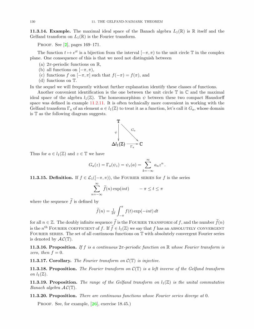
130 11. THE GELFAND-NAIMARK THEOREM
11.3.14. Example. The maximal ideal space of the Banach algebra L1(R) is R itself and theGelfand transform on L1(R) is the Fourier transform.
Proof. See [2], pages 169–171.
The function t 7→ eit is a bijection from the interval [−π, π) to the unit circle T in the complexplane. One consequence of this is that we need not distinguish between
(a) 2π-periodic functions on R,(b) all functions on [−π, π),(c) functions f on [−π, π] such that f(−π) = f(π), and(d) functions on T.
In the sequel we will frequently without further explanation identify these classes of functions.Another convenient identification is the one between the unit circle T in C and the maximal
ideal space of the algebra l1(Z). The homeomorphism ψ between these two compact Hausdorffspace was defined in example 11.2.11. It is often technically more convenient in working with theGelfand transform Γa of an element a ∈ l1(Z) to treat it as a function, let’s call it Ga, whose domainis T as the following diagram suggests.
∆l1(Z) CΓa//
T
∆l1(Z)
ψ
T
C
Ga
Thus for a ∈ l1(Z) and z ∈ T we have
Ga(z) = Γa(ψz) = ψz(a) =∞∑
k=−∞anz
n .
11.3.15. Definition. If f ∈ L1([−π, π)), the Fourier series for f is the series∞∑
n=−∞f(n) exp(int) − π ≤ t ≤ π
where the sequence f is defined by
f(n) = 12π
∫ π
−πf(t) exp(−int) dt
for all n ∈ Z. The doubly infinite sequence f is the Fourier transform of f , and the number f(n)
is the nth Fourier coefficient of f . If f ∈ l1(Z) we say that f has an absolutely convergentFourier series. The set of all continuous functions on T with absolutely convergent Fourier seriesis denoted by AC(T).
11.3.16. Proposition. If f is a continuous 2π-periodic function on R whose Fourier transform iszero, then f = 0.
11.3.17. Corollary. The Fourier transform on C(T) is injective.
11.3.18. Proposition. The Fourier transform on C(T) is a left inverse of the Gelfand transformon l1(Z).
11.3.19. Proposition. The range of the Gelfand transform on l1(Z) is the unital commutativeBanach algebra AC(T).
11.3.20. Proposition. There are continuous functions whose Fourier series diverge at 0.
Proof. See, for example, [26], exercise 18.45.)
11.4. UNITAL C∗-ALGEBRAS 131
What does the preceding result say about the Gelfand transform Γ: l1(Z)→ C(T)?
Suppose a function f belongs to AC(T) and is never zero. Then 1/f is certainly continuouson T, but does it have an absolutely convergent Fourier series? One of the first triumphs of theabstract study of Banach algebras was a very simple proof of the answer to this question givenoriginally by Norbert Wiener. Wiener’s original proof by comparison was quite difficult.
11.3.21. Theorem (Wiener’s theorem). Let f be a continuous function on T which is never zero.If f has an absolutely convergent Fourier series, then so does its reciprocal 1/f .
11.3.22. Example. The Laplace transform can also be viewed as a special case of the Gelfandtransform. For details see [2], pages 173–175.
11.4. Unital C∗-algebras
11.4.1. Proposition. If a is an element of a ∗ -algebra, then σ(a∗) = σ(a).
11.4.2. Proposition. In every C∗-algebra involution is an isometry. That is, ‖a∗‖ = ‖a‖ forevery element a in the algebra.
In definition 3.5.24 of normed algebra we made the special requirement that the identity elementof a unital normed algebra have norm one. In C∗-algebras this requirement is redundant.
11.4.3. Corollary. In a unital C∗-algebra ‖1‖ = 1.
11.4.4. Corollary. Every unitary element in a unital C∗-algebra has norm one.
11.4.5. Corollary. If a is an element of a C∗-algebra A such that ab = 0 for every b ∈ A, thena = 0.
11.4.6. Proposition. Let a be a normal element of a C∗-algebra. Then ‖a2‖ = ‖a‖2. And if thealgebra is unital, then ρ(a) = ‖a‖.
11.4.7. Corollary. If p is a nonzero projection in a C∗-algebra, then ‖p‖ = 1.
11.4.8. Corollary. Let a ∈ A where A is a commutative C∗-algebra. Then ‖a2‖ = ‖a‖2 and ifadditionally A is unital, then ρ(a) = ‖a‖.
11.4.9. Corollary. On a unital commutative C∗-algebra A the Gelfand transform Γ is an isometry;that is, ‖Γa‖u = ‖a‖u = ‖a‖ for every a ∈ A.
11.4.10. Corollary. The norm of a unital C∗-algebra is unique in the sense that given a unitalalgebra A with involution there is at most one norm which makes A into a C∗-algebra.
11.4.11. Proposition. If a is a self-adjoint element of a unital C∗-algebra, then σ(a) ⊆ R.
Hint for proof . Write λ ∈ σ(a) in the form α + iβ where α, β ∈ R. For every n ∈ N letbn := a−α1 + inβ1. Show that for every n the scalar i(n+ 1)β belongs to the spectrum of bn andthat therefore
|i(n+ 1)β|2 ≤ ‖a− α1‖2 + n2β2 .
11.4.12. Corollary. Let A be a unital commutative C∗-algebra. If a ∈ A is self-adjoint, then itsGelfand transform a is real valued.
11.4.13. Corollary. Every character on a unital C∗-algebra is a ∗ -homomorphism.
11.4.14. Corollary. The Gelfand transform on a unital commutative C∗-algebra A is a unital∗ -homomorphism into C(∆A).
11.4.15. Corollary. The range of the Gelfand transform on a unital commutative C∗-algebra A isa unital self-adjoint separating subalgebra of C(∆A).
11.4.16. Proposition. If u is a unitary element of a unital C∗-algebra, then σ(u) ⊆ T.
132 11. THE GELFAND-NAIMARK THEOREM
11.4.17. Proposition. The Gelfand transform Γ is a natural equivalence between the identityfunctor and the C∆ functor on the category of commutative unital C∗-algebras and unital ∗ -homomorphisms.
11.5. The Gelfand-Naimark Theorem
We recall a standard theorem from real analysis.
11.5.1. Theorem (Stone-Weierstrass Theorem). Let X be a compact Hausdorff space. Everyunital separating ∗ -subalgebra of C(X) is dense.
Proof. See [12], theorem 2.40.
The first version of the Gelfand-Naimark theorem says that any unital commutative C∗-algebrais the algebra of all continuous functions on some compact Hausdorff space. Of course the wordis in the preceding sentence means is isometrically ∗ -isomorphic to. The compact Hausdorff spacereferred to is the character space of the algebra.
11.5.2. Theorem (Gelfand-Naimark theorem I). Let A be a unital commutative C∗-algebra. Thenthe Gelfand transform ΓA : a 7→ a is an isometric ∗ -isomorphism of A onto C(∆A).
11.5.3. Definition. Let S be a nonempty subset of a C∗-algebra A. The intersection of the familyof all C∗-subalgebras of A which contain S is the C∗-subalgebra generated by S. We denoteit by C∗(S). (It is easy to see that the intersection of a family of C∗-subalgebras really is a C∗-algebra.) In some cases we shorten the notation slightly: for example, if a ∈ A we write C∗(a)for C∗(a) and C∗(1, a) for C∗(1, a).
11.5.4. Proposition. Let S be a nonempty subset of a C∗-algebra A. For each natural number ndefine the set Wn to be the set of all elements a of A for which there exist x1, x2, . . . , xn in S ∪S∗such that a = x1x2 · · ·xn. Let W =
⋃∞n=1Wn. Then
C∗(S) = spanW .
11.5.5. Theorem (Abstract Spectral Theorem). If a is a normal element of a unital C∗-algebraA, then the C∗-algebra C(σ(a)) is isometrically ∗ -isomorphic to C∗(1, a).
Hint for proof . Use the Gelfand transform of a to identify the maximal ideal space of C∗(1, a)with the spectrum of a. Apply the functor C. Compose the resulting map with Γ−1 where Γ is theGelfand transform on the C∗-algebra C∗(1, a).
If ψ : C(σ(a))→ C∗(1, a) is the ∗ -isomorphism in the preceding theorem and f is a continuousfunction on the spectrum of a, then the element ψ(f) in the algebra A is usually denoted by f(a).This operation of associating with the continuous function f an element f(a) in A is referred to asthe functional calculus associated with a.
11.5.6. Example. Suppose that in the preceding theorem ψ : C(σ(a))→ C∗(1, a) implements theisometric ∗ -isomorphism. Then the image under ψ of the constant function 1 on the spectrum of ais 1A and the image under ψ of the identity function λ 7→ λ on the spectrum of a is a.
11.5.7. Example. Let T be a normal operator on a Hilbert space H whose spectrum is containedin [0,∞). Suppose that ψ : C(σ(T )) → C∗(I, T ) implements the isometric ∗-isomorphism between
these two C∗-algebras. Then there is at least one operator√T whose square is T . Indeed, whenever
f is a continuous function on the spectrum of a normal operator T , we may meaningfully speak ofthe operator f(T ).
11.5.8. Example. If N is a normal Hilbert space operator whose spectrum is 0, 1, then N is anorthogonal projection.
11.5.9. Example. If N is a normal Hilbert space operator whose spectrum is is contained in theunit circle T, then N is a unitary operator.
11.5. THE GELFAND-NAIMARK THEOREM 133
11.5.10. Proposition (Spectral mapping theorem). Let a be a self-adjoint element in a unitalC∗-algebra A and f be a continuous complex valued function on the spectrum of a. Then
σ(f(a)) = f→(σ(a)) .
The functional calculus sends continuous functions to continuous functions in the followingsense.
11.5.11. Proposition. Suppose A is a unital C∗-algebra, K is a nonempty compact subset of R,and f : K → C is a continuous function. Let HK be the set of all self-adjoint elements of A whosespectra are subsets of K. Then the function f : HK → A : h 7→ f(h) is continuous.
Hint for proof . Approximate f uniformly by a polynomial and use an “ε over 3” argument andthe spectral mapping theorem 11.5.10.

CHAPTER 12
SURVIVAL WITHOUT IDENTITY
12.1. Unitization of Banach Algebras
12.1.1. Definition. Let A be an algebra. Define A ./ C to be the set A × C on which additionand scalar multiplication are defined pointwise and multiplication is defined by
(a, λ) · (b, µ) = (ab+ µa+ λb, λµ).
If the algebra A is equipped with an involution, define an involution on A ./ C pointwise; that is,(a, λ)∗ := (a∗, λ). (The notation A ./ C is not standard.)
12.1.2. Proposition. If A is an algebra, then A ./ C is a unital algebra in which A is embeddedas (that is, isomorphic to) an ideal such that (A ./ C)/A ∼= C. The identity of A ./ C is (0, 1). If Ais a ∗ -algebra, then A ./ C is a unital ∗ -algebra in which A is a ∗ -ideal such that (A ./ C)/A ∼= C.
12.1.3. Definition. The algebra A ./ C is the unitization of the algebra (or ∗ -algebra) A.
12.1.4. Notation. In the preceding construction elements of the algebra A ./ C are technicallyordered pairs (a, λ). They are usually written differently. Let ι : A → A ./ C : a 7→ (a, 0) andπ : A ./ C→ C : (a, λ) 7→ λ. It follows, since (0, 1) is the identity in A ./ C, that
(a, λ) = (a, 0) + (0, λ)
= ι(a) + λ1A./C
It is conventional to treat ι as an inclusion mapping. Thus it is reasonable to write (a, λ) asa + λ1A./C or simply as a + λ1. No ambiguity seems to follow from omitting reference to themultiplicative identity, so a standard notation for the pair (a, λ) is a+ λ.
12.1.5. Definition. Let A be a nonunital algebra. Define the spectrum of an element a ∈ A tobe the spectrum of a regarded as an element of A ./ C; that is, σA(a) := σA./C(a).
12.1.6. Definition. Let A be a normed algebra (with or without involution). On the unitizationA ./ C of A define ‖(a, λ)‖ := ‖a‖+ |λ|.12.1.7. Proposition. Let A be a normed algebra. The mapping (a, λ) 7→ ‖a‖+ |λ| defined above isa norm under which A ./ C is a normed algebra. If A is a Banach algebra (respectively, a Banach∗ -algebra), then A ./ C is a Banach algebra (respectively, a Banach ∗ -algebra). The resultingBanach algebra (or Banach ∗ -algebra) is the unitization of A and will be denoted by Ae.
With this expanded definition of spectrum many of the earlier facts for unital Banach algebrasremain true in the more general setting. In particular, for future reference we restate items 8.1.36,8.1.41, 8.1.46, and 8.1.50.
12.1.8. Proposition. Let a be an element of a Banach algebra A. Then the spectrum of a iscompact and |λ| ≤ ‖a‖ for every λ ∈ σ(a).
12.1.9. Proposition. The spectrum of every element of a Banach algebra is nonempty.
12.1.10. Proposition. For every element a of a Banach algebra ρ(a) ≤ ‖a‖ and ρ(an) =(ρ(a)
)n.
12.1.11. Theorem (Spectral radius formula). If a is an element of a Banach algebra, then
ρ(a) = inf‖an‖1/n : n ∈ N
= lim
n→∞‖an‖1/n.
135
136 12. SURVIVAL WITHOUT IDENTITY
12.1.12. Definition. Let A be an algebra. A left ideal J in A is a modular left ideal if thereexists an element u in A such that au − a ∈ J for every a ∈ A. Such an element u is called aright identity with respect to J . Similarly, a right ideal J in A is a modular right idealif there exists an element v in A such that va− a ∈ J for every a ∈ A. Such an element v is calleda left identity with respect to J . A two-sided ideal J is a modular ideal if there existsan element e which is both a left and a right identity with respect to J .
12.1.13. Proposition. An ideal J in an algebra is modular if and only if it is both left modularand right modular.
Hint for proof . Show that if u is a right identity with respect to J and v is a left identity withrespect to J , then vu is both a right and left identity with respect to J .
12.1.14. Proposition. An ideal J in an algebra A is modular if and only if the quotient algebraA/J is unital.
12.1.15. Example. Let X be a locally compact Hausdorff space. For every x ∈ X the ideal Jx isa maximal modular ideal in the C∗-algebra C0(X) of continuous complex valued functions on X.
Proof. By the locally compact Hausdorff space version of Urysohn’s lemma (see, for example,[16], theorem 17.2.10) there exists a function g ∈ C0(X) such that g(x) = 1. Thus Jx is mod-ular because g is an identity with respect to Jx. Since C0(X) = Jx ⊕ spang the ideal Jx hascodimension 1 and is therefore maximal.
12.1.16. Proposition. If J is a proper modular ideal in a Banach algebra, then so is its closure.
12.1.17. Corollary. Every maximal modular ideal in a Banach algebra is closed.
12.1.18. Proposition. Every proper modular ideal in a Banach algebra is contained in a maximalmodular ideal.
12.1.19. Proposition. Let A be a commutative Banach algebra and φ ∈ ∆A. Then kerφ is amaximal modular ideal in A and A/ kerφ is a field. Furthermore, every maximal modular ideal isthe kernel of exactly one character in ∆A.
12.1.20. Proposition. Every multiplicative linear functional on a commutative Banach algebra Ais continuous. In fact, every character is contractive.
12.1.21. Example. Let Ae be the unitization of a commutative Banach algebra A (see proposi-tion 12.1.7). Define
φ∞ : Ae → C : (a, λ) 7→ λ .
Then φ∞ is a character on Ae.
12.1.22. Proposition. Every character φ on a commutative Banach algebra A has a unique ex-tension to a character φe on the unitization Ae of A. And the restriction to A of any character onAe, with the obvious exception of φ∞, is a character on A.
12.1.23. Proposition. If A is a commutative Banach algebra, then
(a) ∆A is a locally compact Hausdorff space,(b) ∆Ae = ∆A ∪ φ∞,(c) ∆Ae is the one-point compactification of ∆A, and(d) the map φ 7→ φe is a homeomorphism from ∆A onto ∆Ae \ φ∞.
If A is unital (so that ∆A is compact), then φ∞ is an isolated point of ∆Ae.
12.1.24. Theorem. If A is a commutative Banach algebra with a nonempty character space, thenthe Gelfand transform
Γ = ΓA : C0(∆A) : a 7→ a = Γais a contractive algebra homomorphism and ρ(a) = ‖a‖u. Furthermore, if A is not unital, thenσ(a) = ran a ∪ 0 for every a ∈ A.
12.2. EXACT SEQUENCES AND EXTENSIONS 137
12.2. Exact Sequences and Extensions
The rather simple procedure for the unitization of Banach ∗ -algebras (see 12.1.1 and 12.1.6)does not carry over to C∗-algebras. The norm defined in 12.1.6 does not satisfy the C∗-condition(definition 7.1.23). It turns out that the unitization of C∗-algebras is a bit more complicated. Beforeexamining the details we look at some preparatory material on exact sequences and extensions ofC∗-algebras.
In the world of C∗-algebras exact sequences are defined in essentially the same way as exactsequences of Banach algebras (see 6.5.9).
12.2.1. Definition. A sequence of C∗-algebras and ∗ -homomorphisms
· · · // An−1φn // An
φn+1 // An+1// · · ·
is said to be exact at An if ranφn = kerφn+1. A sequence is exact if it is exact at each of itsconstituent C∗-algebras. A sequence of C∗-algebras and ∗ -homomorphisms of the form
0 // Aφ // E
ψ // B // 0 (12.2.1)
is a short exact sequence. (Here 0 denotes the trivial 0-dimensional C∗-algebra, and the unla-beled arrows are the obvious ∗-homomorphisms.) The short exact sequence of C∗-algebras (6.5.1)is split exact if there exists a ∗ -homomorphism ξ : B → E such that ψ ξ = idB.
The preceding definitions were for the category CSA of C∗-algebras and ∗ -homomorphisms.Of course there is nothing special about this particular category. Exact sequences make sense inmany situations, in, for example, various categories of Banach spaces, Banach algebras, Hilbertspaces, vector spaces, Abelian groups, modules, and so on.
Often in the context of C∗-algebras the exact sequence (6.5.1) is referred to as an extension.Some authors refer to it as an extension of A by B (for example, [51] and [10]) while others sayit is an extension of B by A ([39], [18], and [3]). In [18] and [3] the extension is defined to bethe sequence 6.5.1; in [51] it is defined to be the ordered triple (φ,E, ψ); and in [39] and [10] it isdefined to be the C∗-algebra E itself. Regardless of the formal definitions it is common to say thatE is an extension of A by B (or of B by A).
12.2.2. Convention. In a C∗-algebra the word ideal will always mean a closed two-sided ∗ -ideal(unless, of course, the contrary is explicitly stated). We will show shortly (in proposition 12.6.6)that requiring an ideal in a C∗-algebra to be self-adjoint is redundant. A two-sided algebra idealof a C∗-algebra which is not necessarily closed will be called an algebraic ideal. A self-adjointalgebraic ideal of a C∗-algebra will be called an algebraic ∗-ideal.
Compare the next two propositions to the nearly identical 6.5.10 and 6.5.11.
12.2.3. Proposition. Consider the following diagram in the category of C∗-algebras and ∗-homomorphisms
0 // A
f
j // B
g
k // C
h
// 0
0 // A′j′// B′
k′// C ′ // 0
If the rows are exact and the left square commutes, then there exists a unique ∗-homomorphismh : C → C ′ which makes the right square commute.
138 12. SURVIVAL WITHOUT IDENTITY
12.2.4. Proposition (The Five Lemma). Suppose that in the following diagram of C∗-algebrasand ∗-homomorphisms
0 // A
f
j // B
g
k // C
h
// 0
0 // A′j′// B′
k′// C ′ // 0
the rows are exact and the squares commute. Prove the following.
(a) If g is surjective, so is h.(b) If f is surjective and g is injective, then h is injective.(c) If f and h are surjective, so is g.(d) If f and h are injective, so is g.
12.2.5. Definition. Let A and B be C∗-algebras. We define the (external) direct sum of Aand B, denoted by A ⊕ B, to be the Cartesian product A × B with pointwise defined algebraicoperations and norm given by
‖(a, b)‖ = max‖a‖, ‖b‖for all a ∈ A and b ∈ B. An alternative notation for the element (a, b) in A⊕B is a⊕ b.12.2.6. Example. Let A and B be C∗-algebras. Then the direct sum of A and B is a C∗-algebraand the following sequence is split short exact:
0 // Aι1 // A⊕B π2 // B // 0
The indicated maps in the preceding are the obvious ones:
ι1 : A→ A⊕B : a 7→ (a,0) and π2 : A⊕B → B : (a, b) 7→ b .
This is the direct sum extension.
12.2.7. Proposition. If A and B are nonzero C∗-algebras, then their direct sum A⊕B is a productin the category CSA of C∗-algebras and ∗ -homomorphisms (see example 4.7.15). The direct sumis unital if and only if both A and B are.
12.2.8. Definition. Let A and B be C∗-algebras and E and E′ be extensions of A by B. Theseextensions are strongly equivalent if there exists a ∗-isomorphism θ : E → E′ that makes thediagram
0 // A // E //
θ
B // 0
0 // A // E′ // B // 0commute.
12.2.9. Proposition. In the preceding definition it is enough to require θ to be a ∗-homomorphism.
12.2.10. Proposition. Let A and B be C∗-algebras. An extension
0 // Aφ // E
ψ // B // 0
is strongly equivalent to the direct sum extension A⊕B if and only if there exists a ∗-homomorphismν : E → A such that ν φ = idA.
12.2.11. Proposition. If the sequences of C∗-algebras
0 // Aφ // E
ψ // B // 0 (12.2.2)
and
0 // Aφ′ // E′
ψ′ // B // 0 (12.2.3)
are strongly equivalent and (12.2.2) splits, then so does (12.2.3).
12.3. UNITIZATION OF C∗-ALGEBRAS 139
12.3. Unitization of C∗-algebras
The rather simple procedure for the unitization of Banach ∗ -algebras (see 12.1.1 and 12.1.6)does not carry over to C∗-algebras. The norm defined in 12.1.6 does not satisfy the C∗-condition(definition 7.1.23). It turns out that the unitization of C∗-algebras is a bit more complicated.
12.3.1. Proposition. The kernel of a ∗ -homomorphism φ : A→ B between C∗-algebras is a closed∗ -ideal in A and its range is a ∗ -subalgebra of B.
12.3.2. Proposition. If a is an element in a C∗-algebra, then
‖a‖ = sup‖xa‖ : ‖x‖ ≤ 1= sup‖ax‖ : ‖x‖ ≤ 1.
12.3.3. Corollary. If a is an element of a C∗-algebra A, the operator La, called left multipli-cation by a and defined by
La : A→ A : x 7→ ax
is a (bounded linear) operator on A. Furthermore, the map
L : A→ B(A) : a 7→ La
is both an isometry and an algebra homomorphism.
12.3.4. Proposition. Let A be a C∗-algebra. Then there exists a unital C∗-algebra A in which Ais embedded as an ideal such that the sequence
0 // A // A // C // 0 (12.3.1)
is split exact. If A is unital then the sequence (12.3.1) is strongly equivalent to the direct sum
extension, so that A ∼= A⊕ C. If A is not unital, then A is not isomorphic to A⊕ C.
Hint for proof . The proof this result is a little complicated. Everyone should go through allthe details at least once in his/her life. What follows is an outline of a proof.
Notice that we speak of the unitization of C∗-algebra A whether or not A already has a unit(multiplicative identity). We divide the argument into two cases.
Case 1: the algebra A is unital.
(a) On the algebra A ./ C define
‖(a, λ)‖ := max‖a+ λ1A‖, |λ|
and let A := A ./ C together with this norm.(b) Prove that the map (a, λ) 7→ ‖(a, λ)‖ is a norm on A ./ C.(c) Prove that this norm is an algebra norm.(d) Show that it is, in fact, a C∗-norm on A ./ C.(e) Observe that it is an extension of the norm on A.(f) Prove that A ./ C is a C∗-algebra by verifying completeness of the metric space induced
by the preceding norm.(g) Prove that the sequence
0 // Aι // A
Q //ooψ
C // 0
is split exact (where ι : a 7→ (a, 0), Q : (a, λ) 7→ λ, and ψ : λ 7→ (0, λ)).
(h) Prove that A∗∼= A⊕ C.
Case 2: the algebra A is not unital.
(i) Prove the following simple fact.
140 12. SURVIVAL WITHOUT IDENTITY
12.3.5. Lemma. Let A be an algebra and B be a normed algebra. If φ : A → B is analgebra homomorphism, the function a 7→ ‖a‖ := ‖φ(a)‖ is a seminorm on A. The functionis a norm if φ is injective.
(j) Recall that we defined the operator La, left multiplication by a, in 12.3.3. Now let
A] := La + λIA ∈ B(A) : a ∈ A and λ ∈ Cand show that A] is a normed algebra.
(k) Make A] into a ∗ -algebra by defining
(La + λIA)∗ := La∗ + λIA
for all a ∈ A and λ ∈ C.(l) Define
φ : A ./ C→ A] : (a, λ) 7→ La + λIA
and verify that φ is a ∗ -homomorphism.(m) Prove that φ is injective.(n) Use (9) to endow A ./ C with a norm which makes it into a unital normed algebra. Let
A := A ./ C with the norm pulled back by φ from A]
(o) Verify the following facts.
(a) The map φ : A→ A] is an isometric isomorphism.(b) ranL is a closed subalgebra of ranφ = A] ⊆ B(A).(c) IA /∈ ranL.
(p) Prove that the norm on A satisfies the C∗-condition.
(q) Prove that A is a unital C∗-algebra. (To show that A is complete we need only show that A]
is complete. To this end let(φ(an, λn)
)∞n=1
be a Cauchy sequence in A]. To show that thissequence converges it suffices to show that it has a convergent subsequence. Showing thatthe sequence (λn) is bounded allows us to extract from it a convergent subsequence
(λnk).
Prove that (Lank ) converges.)
(r) Prove that the sequence
0 // A // A // C // 0 (12.3.2)
is split exact.
(s) The C∗-algebra A is not equivalent to A⊕ C.
12.3.6. Definition. The C∗-algebra A constructed in the preceding proposition is the unitizationof A.
Note that the expanded definition of spectrum given in 12.1.5 applies to C∗-algebras since theadded identity is purely an algebraic matter and is the same for C∗-algebras as it is for generalBanach algebras. Thus many of the earlier facts stated for unital C∗-algebras remain true. Inparticular, for future reference we restate items 11.4.6, 11.4.8, 11.4.9, 11.4.10, 11.4.11, 11.4.12,and 11.4.13.
12.3.7. Proposition. Let a be a normal element of a C∗-algebra. Then ‖a2‖ = ‖a‖2 and thereforeρ(a) = ‖a‖.
12.3.8. Corollary. If A is a commutative C∗-algebra, then ‖a2‖ = ‖a‖2 and ρ(a) = ‖a‖ for everya ∈ A.
12.3.9. Corollary. On a commutative C∗-algebra A the Gelfand transform Γ is an isometry; thatis, ‖Γa‖u = ‖a‖u = ‖a‖ for every a ∈ A.
12.3.10. Corollary. The norm of a C∗-algebra is unique in the sense that given a algebra A withinvolution there is at most one norm which makes A into a C∗-algebra.
12.3. UNITIZATION OF C∗-ALGEBRAS 141
12.3.11. Proposition. If h is a self-adjoint element of a C∗-algebra, then σ(h) ⊆ R.
12.3.12. Proposition. If a is a self-adjoint element in a C∗-algebra, then its Gelfand transforma is real valued.
12.3.13. Proposition. Every character on a C∗-algebra A preserves involution, thus the Gelfandtransform Γ
Ais a ∗-homomorphism.
An immediate result of the preceding results is the second version of the Gelfand-Naimarktheorem, which says that any commutative C∗-algebra is (isometrically unitally ∗ -isomorphic to)the algebra of all those continuous functions on some locally compact Hausdorff space which vanishat infinity. As was the case with the first version of this theorem (see 11.5.2) the locally compactHausdorff space referred to is the character space of the algebra.
12.3.14. Theorem (Gelfand-Naimark Theorem II). Let A be a commutative C∗-algebra. Thenthe Gelfand transform ΓA : a 7→ a is an isometric unital ∗ -isomorphism of A onto C0(∆A).
It follows from the next proposition that the unitization process is functorial.
12.3.15. Proposition. Every ∗-homomorphism φ : A → B between C∗-algebras has a unique ex-
tension to a unital ∗-homomorphism φ : A→ B between their unitizations.
In contrast to the situation in general Banach algebras there is no distinction between topo-logical and geometric categories of C∗-algebras. One of the most remarkable aspects of C∗-algebratheory is that ∗-homomorphisms between such algebras are automatically continuous—in fact, con-tractive. It follows that if two C∗-algebras are algebraically ∗-isomorphic, then they are isometricallyisomorphic.
12.3.16. Proposition. Every ∗-homomorphism between C∗-algebras is contractive.
12.3.17. Proposition. Every injective ∗-homomorphism between C∗-algebras is an isometry.
12.3.18. Proposition. Let X be a locally compact Hausdorff space and X = X ∪ ∞ be itsone-point compactification. Define
ι : C0(X)→ C(X) : f 7→ f
where
f(x) =
f(x), if x ∈ X;0, if x =∞.
Also let E∞ be defined on C(X) by E∞(g) = g(∞). Then the sequence
0 // C0(X)ι // C(X)
E∞ // C // 0
is exact.
In the preceding proposition we refer to X as the one-point compactification of X even in thecase that X is compact to begin with. Most definitions of compactification require a space to bedense in any compactification. (See my remarks in the beginning of section 17.3 of [16].) We havepreviously adopted the convention that the unitization of a unital algebra gets a new multiplicativeidentity. In the spirit of consistency with this choice we will in the sequel subscribe to the conventionthat the one-point compactification of a compact space gets an additional (isolated) point. (Seealso the terminology we introduce in 14.3.1.)
From the point of view of the Gelfand-Naimark theorem (12.3.14) the fundamental insightprompted by the next proposition is that the unitization of a commutative C∗-algebra is, in somesense, the “same thing” as the one-point compactification of a locally compact Hausdorff space.
12.3.19. Proposition. If X is a locally compact Hausdorff space, then the unital C∗-algebras(C0(X)
)∼and C(X) are isometrically ∗ -isomorphic.
142 12. SURVIVAL WITHOUT IDENTITY
Proof. Define
θ :(C0(X)
)∼→ C(X) : (f, λ) 7→ f + λ1X
(where 1X
is the constant function 1 on X). Then consider the diagram
0 // C0(X) //(C0(X)
)∼ //
θ
C // 0
0 // C0(X)ι // C(X)
E∞ // C // 0
The top row is exact by proposition 12.3.4, the bottom row is exact by proposition 12.3.18, andthe diagram obviously commutes. It is routine to check that θ is a ∗ -homomorphism. Therefore θis an isometric ∗ -isomorphism by proposition 12.2.9 and corollary 12.3.17.
12.4. Quasi-inverses
12.4.1. Definition. An element b of an algebra A is a left quasi-inverse for a ∈ A if ba = a+b.It is a right quasi-inverse for a if ab = a + b. If b is both a left and a right quasi-inverse for ait is a quasi-inverse for a. When a has a quasi-inverse denote it by a′.
12.4.2. Proposition. If b is a left quasi-inverse for a in an algebra A and c is a right quasi-inversefor a in A, then b = c.
12.4.3. Proposition. Let A be a unital algebra and let a, b ∈ A. Then
(a) a′ exists if and only if (1− a)−1 exists; and(b) b−1 exists if and only if (1− b)′ exists.
Hint for proof . For the reverse direction in (a) consider a+ c− ac where c = 1− (1− a)−1.
12.4.4. Proposition. An element a of a Banach algebra A is quasi-invertible if and only if it isnot an identity with respect to any maximal modular ideal in A.
12.4.5. Proposition. Let A be a Banach algebra and a ∈ A. If ρ(a) < 1, then a′ exists anda′ = −
∑∞k=1 a
k.
12.4.6. Proposition. Let A be a Banach algebra and a ∈ A. If ‖a‖ < 1, then a′ exists and
‖a‖1 + ‖a‖
≤ ‖a′‖ ≤ ‖a‖1− ‖a‖
.
12.4.7. Proposition. Let A be a unital Banach algebra and a ∈ A. If ρ(1 − a) < 1, then a isinvertible in A.
12.4.8. Proposition. Let A be a Banach algebra and a, b ∈ A. If b′ exists and ‖a‖ < (1+‖b′‖)−1,then (a+ b)′ exists and
‖(a+ b)′ − b′‖ ≤ ‖a‖ (1 + ‖b′‖)2
1− ‖a‖ (1 + ‖b′‖).
Hint for proof . Show first that u = (a− b′a)′ exists and that u+ b′ − ub′ is a left quasi-inversefor a + b.
Compare the next result with propositions 8.1.33 and 8.1.34
12.4.9. Proposition. The set QA of quasi-invertible elements of a Banach algebra A is open inA, and the map a 7→ a′ is a homeomorphism of QA onto itself.
12.4.10. Notation. If a and b are elements in an algebra we define a b := a+ b− ab.
12.4.11. Proposition. If A is an algebra, then QA is a group under .
12.5. POSITIVE ELEMENTS IN C∗-ALGEBRAS 143
12.4.12. Proposition. If A is a unital Banach algebra and invA is the set of its invertible ele-ments, then
Ψ: QA → invA : a 7→ 1− ais an isomorphism.
12.4.13. Definition. If A is a algebra and a ∈ A, we define the q-spectrum of a in A by
σA(a) := λ ∈ C : λ 6= 0 anda
λ/∈ QA ∪ 0.
In a unital algebra, the preceding definition is “almost” the usual one.
12.4.14. Proposition. Let A be a unital algebra and a ∈ A. Then for all λ 6= 0, we have λ ∈ σ(a)if and only if λ ∈ σ(a).
12.4.15. Proposition. If an algebra A is not unital and a ∈ A, then σA(a) = σA
(a), where A isthe unitization of A.
12.5. Positive Elements in C∗-algebras
12.5.1. Definition. A self-adjoint element a of a C∗-algebra A is positive if σ(a) ⊆ [0,∞). Inthis case we write a ≥ 0. We denote the set of all positive elements of A by A+. This is thepositive cone of A. For any subset B of A let B+ = B ∩ A+. We will use the positive cone toinduce a partial ordering on A: we write a ≤ b when b− a ∈ A+.
12.5.2. Definition. Let ≤ be a relation on a nonempty set S. If the relation ≤ is reflexive andtransitive, it is a preordering. If ≤ is a preordering and is also antisymmetric, it is a partialordering.
A partial ordering ≤ on a real vector space V is compatible with (or respects) the operations(addition and scalar multiplication) on V if for all x, y, z ∈ V
(a) x ≤ y implies x+ z ≤ y + z, and(b) x ≤ y, α ≥ 0 imply αx ≤ αy.
A real vector space equipped with a partial ordering which is compatible with the vector spaceoperations is an ordered vector space.
12.5.3. Definition. Let V be a vector space. A subset C of V is a cone in V if αC ⊆ C for everyα ≥ 0. A cone C in V is proper if C ∩ (−C) = 0.
12.5.4. Proposition. A cone C in a vector space is convex if and only if C + C ⊆ C.
12.5.5. Example. If V is an ordered vector space, then the set
V + := x ∈ V : x ≥ 0
is a proper convex cone in V . This is the positive cone of V and its members are the positiveelements of V .
12.5.6. Proposition. Let V be a real vector space and C be a proper convex cone in V . Definex ≤ y if y − x ∈ C. Then the relation ≤ is a partial ordering on V and is compatible with thevector space operations on V . This relation is the partial ordering induced by the cone C.The positive cone V + of the resulting ordered vector space is just C itself.
12.5.7. Proposition. If a is a self-adjoint element of a unital C∗-algebra and t ∈ R, then
(i) a ≥ 0 whenever ‖a− t1‖ ≤ t; and(ii) ‖a− t1‖ ≤ t whenever ‖a‖ ≤ t and a ≥ 0.
12.5.8. Example. The positive cone of a C∗-algebra A is a closed proper convex cone in the realvector space H(A).
144 12. SURVIVAL WITHOUT IDENTITY
12.5.9. Proposition. If a and b are positive elements of a C∗-algebra and ab = ba, then ab ispositive.
12.5.10. Proposition. Every positive element of a C∗-algebra A has a unique positive nth root(n ∈ N). That is, if a ∈ A+, then there exists a unique b ∈ A+ such that bn = a.
Proof. Hint. The existence part is a simple application of the C∗-functional calculus (thatis, the abstract spectral theorem 11.5.5). The element b given by the functional calculus is positivein the algebra C∗(1, a). Explain why it is also positive in A. The uniqueness argument deservesconsiderable care.
12.5.11. Theorem (Jordan Decomposition). If c is a self-adjoint element of a C∗-algebra A, thenthere exist positive elements c+ and c− of A such that c = c+ − c− and c+c− = 0.
12.5.12. Lemma. If c is an element of a C∗-algebra such that −c∗c ≥ 0, then c = 0.
12.5.13. Proposition. If a is an element of a C∗-algebra, then a∗a ≥ 0.
12.5.14. Proposition. If c is an element of a C∗-algebra, then the following are equivalent:
(i) c ≥ 0;(ii) there exists b ≥ 0 such that c = b2; and
(iii) there exists a ∈ A such that c = a∗a,
12.5.15. Example. If T is an operator on a Hilbert space H, then T is a positive member of theC∗-algebra B(H) if and only if 〈Tx, x〉 ≥ 0 for all x ∈ H.
Hint for proof . Showing that if T ≥ 0 in B(H), then 〈Tx, x〉 ≥ 0 for all x ∈ H is easy: useproposition 12.5.14 to write T as S∗S for some operator S.
For the converse suppose that 〈Tx, x〉 ≥ 0 for all x ∈ H. It is easy to see that this impliesthat T is self-adjoint. Use the Jordan decomposition theorem12.5.11 to write T as T+ − T−. Forarbitrary u ∈ H let x = T−u and verify that 0 ≤ 〈Tx, x〉 = −〈(T−)3u, u〉. Now (T−)3 is a positiveelement of B(H). (Why?) Conclude that (T−)3 = 0 and therefore T− = 0. (For additional detailsee [11], page 37.)
12.5.16. Definition. For an arbitrary element a of a C∗-algebra we define |a| to be√a∗a.
12.5.17. Proposition. If a is a self-adjoint element of a C∗-algebra, then
|a| = a+ + a− .
12.5.18. Example. The absolute value in a C∗-algebra need not be subadditive; that is, |a + b|
need not be less than |a| + |b|. For example, in M2(C) take a =
[1 11 1
]and b =
[0 00 −2
]. Then
|a| = a, |b| =[0 00 2
], and |a + b| =
[√2 0
0√
2
]. If |a + b| − |a| − |b| were positive, then, according
to example 12.5.15, 〈 (|a+ b| − |a| − |b|)x , x 〉 would be positive for every vector x ∈ C2. But thisis not true for x = (1, 0).
12.5.19. Proposition. If φ : A→ B is a ∗ -homomorphism between C∗-algebras, then φ(a) ∈ B+
whenever a ∈ A+. If φ is a ∗ -isomorphism, then φ(a) ∈ B+ if and only if a ∈ A+.
12.5.20. Proposition. Let a be a self-adjoint element of a C∗-algebra A and f a continuouscomplex valued function on the spectrum of a. Then f ≥ 0 in C(σ(a)) if and only if f(a) ≥ 0 in A.
12.5.21. Proposition. If a is a self-adjoint element of a C∗-algebra A, then ‖a‖1A ± a ≥ 0.
12.5.22. Proposition. If a and b are self-adjoint elements of a C∗-algebra A and a ≤ b, thenx∗ax ≤ x∗bx for every x ∈ A.
12.5.23. Proposition. If a and b are elements of a C∗-algebra with 0 ≤ a ≤ b, then ‖a‖ ≤ ‖b‖.
12.6. APPROXIMATE IDENTITIES 145
12.5.24. Proposition. Let A be a unital C∗-algebra and c ∈ A+. Then c is invertible if and onlyif c ≥ ε1 for some ε > 0.
12.5.25. Proposition. Let A be a unital C∗-algebra and c ∈ A. If c ≥ 1, then c is invertible and0 ≤ c−1 ≤ 1.
12.5.26. Proposition. If a is a positive invertible element in a unital C∗-algebra, then a−1 ispositive.
Next we show that the notation a−12 is unambiguous.
12.5.27. Proposition. Let a ∈ A+ where A is a unital C∗-algebra. If a is invertible, so is a12 and(
a12
)−1=(a−1) 1
2 .
12.5.28. Corollary. If a is an invertible element in a unital C∗-algebra, then so is |a|.
12.5.29. Proposition. Let a and b be elements of a C∗-algebra. If 0 ≤ a ≤ b and a is invertible,then b is invertible and b−1 ≤ a−1.
12.5.30. Proposition. If a and b are elements of a C∗-algebra and 0 ≤ a ≤ b, then√a ≤√b.
12.5.31. Example. Let a and b be elements of a C∗-algebra with 0 ≤ a ≤ b. It is not necessarilythe case that a2 ≤ b2.
Hint for proof . In the C∗-algebra M2 let a =
[1 00 0
]and b = a+ 1
2
[1 11 1
].
12.6. Approximate Identities
12.6.1. Definition. An approximate identity (or approximate unit) in a C∗-algebra A isan increasing net (eλ)λ∈Λ of positive elements of A such that ‖eλ‖ ≤ 1 and aeλ → a (equivalently,eλ a→ a) for every a ∈ A. If such a net is in fact a sequence, we have a sequential approximateidentity. In the literature be careful of varying definitions: many authors omit the requirementsthat the net be increasing and/or that it be bounded.
12.6.2. Example. Let A = C0(R). For each n ∈ N let Un = (−n, n) and let en : R → [0, 1] be afunction in A whose support is contained in Un+1 and such that en(x) = 1 for every x ∈ Un. Then(en) is a (sequential) approximate identity for A.
12.6.3. Proposition. If A is a C∗-algebra, then the set
Λ := a ∈ A+ : ‖a‖ < 1is a directed set (under the ordering it inherits from H(A)).
Hint for proof . Verify that the function
f : [0, 1)→ R+ : t 7→ (1− t)−1 − 1 =t
1− tinduces an order isomorphism f : Λ → A+. (An order isomorphism between partially orderedsets is an order preserving bijection whose inverse also preserves order.) A careful proof of thisresult involves checking a rather large number of details.
12.6.4. Proposition. If A is a C∗-algebra, then the set
Λ := a ∈ A+ : ‖a‖ < 1is an approximate identity for A.
12.6.5. Corollary. Every C∗-algebra A has an approximate identity. If A is separable then it hasa sequential approximate identity.
12.6.6. Proposition. Every closed (two-sided) algebraic ideal in a C∗-algebra is self-adjoint.
146 12. SURVIVAL WITHOUT IDENTITY
12.6.7. Proposition. If J is an ideal in a C∗-algebra A, then A/J is a C∗-algebra.
Proof. See [27], theorem 1.7.4, or [10], pages 13–14, or [18], theorem 2.5.4.
12.6.8. Example. If J is an ideal in a C∗-algebra A, then the sequence
0 // J // Aπ // A/J // 0
is short exact.
12.6.9. Proposition. The range of a ∗-homomorphism between C∗-algebras is closed (and thereforeitself a C∗-algebra).
12.6.10. Definition. A C∗-subalgebra B of a C∗-algebra A is hereditary if a ∈ B whenevera ∈ A, b ∈ B, and 0 ≤ a ≤ b.12.6.11. Proposition. Suppose x∗x ≤ a in a C∗-algebra A. Then there exists b ∈ A such that
x = ba14 and ‖b‖ ≤ ‖a‖
14 .
Proof. See [10], page 13.
12.6.12. Proposition. Suppose J is an ideal in a C∗-algebra A, j ∈ J+, and a∗a ≤ j. Thena ∈ J . Thus ideals in C∗-algebras are hereditary.
12.6.13. Theorem. Let A and B be C∗-algebras and J be an ideal in A. If φ is a ∗ -homomorphism
from A to B and kerφ ⊇ J , then there exists a unique ∗ -homomorphism φ : A/J → B which makesthe following diagram commute.
A
π
φ
A/J
φ
// B
Furthermore, φ is injective if and only if kerφ = J ; and φ is surjective if and only if φ is.
12.6.14. Corollary. If 0 // Aφ // E // B // 0 is a short exact sequence of C∗-algebras,
then E/ ranφ and B are isometrically ∗ -isomorphic.
12.6.15. Corollary. Every C∗-algebra A has codimension one in its unitization A; that is, dim A/A =1.
12.6.16. Proposition. Let A be a C∗-algebra, B be a C∗-subalgebra of A, and J be an ideal in A.Then
B/(B ∩ J) ∼= (B + J)/J .
Let B be a unital subalgebra of an arbitrary algebra A. It is clear that if an element b ∈ B isinvertible in B, then it is also invertible in A. The converse turns out to be true in C∗-algebras: ifb is invertible in A, then its inverse lies in B. This is usually expressed by saying that every unitalC∗-subalgebra of a C∗-algebra is inverse closed.
12.6.17. Proposition. Let B be a unital C∗-subalgebra of a C∗-algebra A. If b ∈ inv(A), thenb−1 ∈ B.
12.6.18. Corollary. Let B be a unital C∗-subalgebra of a C∗-algebra A and b ∈ B. Then
σB(b) = σA(b) .
12.6.19. Corollary. Let φ : A → B be a unital C∗-monomorphism of a C∗-algebra A and a ∈ A.Then
σ(a) = σ(φ(a)) .
CHAPTER 13
THE GELFAND-NAIMARK-SEGAL CONSTRUCTION
13.1. Positive Linear Functionals
13.1.1. Definition. Let A be an algebra with involution. For each linear functional τ on A andeach a ∈ A define τ?(a) = τ(a∗). We say that τ is Hermitian if τ? = τ . Notice that a linearfunctional τ : A→ C is Hermitian if and only if it preserves involution; that is, τ? = τ if and onlyif τ(a∗) = τ(a) for all a ∈ A.
CAUTION. The τ? defined above should not be confused with the usual adjoint mapping τ∗ : C∗ →A∗. Context (or use of a magnifying glass) should make it clear which is intended.
13.1.2. Proposition. A linear functional τ on a C∗-algebra A is Hermitian if and only if τ(a) ∈ Rwhenever a is self-adjoint.
As is always the case with maps between ordered vector spaces, positive maps are the ones thattake positive elements to positive elements.
13.1.3. Definition. A linear functional τ on a C∗-algebra A is positive if τ(a) ≥ 0 whenevera ≥ 0 in A for all a ∈ A.
13.1.4. Proposition. Every positive linear functional on a C∗-algebra is Hermitian.
13.1.5. Proposition. The family of positive linear functionals is a proper convex cone in the realvector space of all Hermitian linear functionals on a C∗-algebra. The cone induces a partial orderingon the vector space: τ1 ≤ τ2 whenever τ2 − τ1 is positive.
13.1.6. Definition. A state of a C∗-algebra A is a positive linear functional τ on A such thatτ(1) = 1.
13.1.7. Example. Let x be a vector in a Hilbert space H. Define
ωx : B(H)→ C : T 7→ 〈Tx, x〉 .Then ωx is a positive linear functional on B(H). If x is a unit vector, then ωx is a state of B(H).A state τ is a vector state if τ = ωx for some unit vector x.
13.1.8. Proposition (Schwarz inequality). If τ is a positive linear functional on a C∗-algebra A,then
|τ(b∗a)|2 ≤ τ(a∗a)τ(b∗b)
for all a, b ∈ A.
13.1.9. Proposition. A linear functional τ on a C∗-algebra A is positive if and only if it is boundedand ‖τ‖ = τ(1A).
Proof. See [32], pages 256–257.
13.2. Representations
13.2.1. Definition. Let A be a C∗-algebra. A representation of A is a pair (π,H) where His a Hilbert space and π : A → B(H) is a ∗ -homomorphism. Usually one says simply that π is arepresentation of A. When we wish to emphasize the role of the particular Hilbert space we saythat π is a representation of A on H. Depending on context we may write either πa or π(a) for
147
148 13. THE GELFAND-NAIMARK-SEGAL CONSTRUCTION
the Hilbert space operator which is the image of the algebra element a under π. A representationπ of A on H is nondegenerate if π(A)H is dense in H.
13.2.2. Convention. We add to the preceding definition the following requirement: if the C∗-algebra A is unital, then a representation of A must be a unital ∗ -homomorphism.
13.2.3. Definition. A representation π of a C∗-algebra A on a Hilbert space H is faithful if itis injective. If there exists a vector x ∈ H such that π→(A)x = πa(x) : a ∈ A is dense in H, thenwe say that the representation π is cyclic and that x is a cyclic vector for π.
13.2.4. Example. Let (S,A, µ) be a σ-finite measure space and L∞ = L∞(S,A, µ) be the C∗-algebra of essentially bounded µ-measurable functions on S. As we saw in example 5.2.15 foreach φ ∈ L∞ the corresponding multiplication operator Mφ is an operator on the Hilbert spaceL2 = L2(S,A, µ). The mapping M : L∞ → B(L2) : φ 7→ Mφ is a faithful representation of theC∗-algebra L∞ on the Hilbert space L2.
13.2.5. Example. Let C([0, 1]) be the C∗-algebra of continuous functions on the interval [0, 1]. Foreach φ ∈ C([0, 1]) the corresponding multiplication operator Mφ is an operator on the Hilbert spaceL2 = L2([0, 1]) of functions on [0, 1] which are square-integrable with respect to Lebesgue measure.The mapping M : C([0, 1])→ B(L2) : φ 7→Mφ is a faithful representation of the C∗-algebra C([0, 1])on the Hilbert space L2.
13.2.6. Example. Suppose that π is a representation of a unital C∗-algebra A on a Hilbert space Hand x is a unit vector in H. If ωx is the corresponding vector state of B(H), then ωx π is a stateof A.
13.2.7. Exercise. Let X be a locally compact Hausdorff space. Find an isometric (thereforefaithful) representation (π,H) of the C∗-algebra C0(X) on some Hilbert space H..
13.2.8. Definition. Let ρ be a state of a C∗-algebra A. Then
Lρ := a ∈ A : ρ(a∗a) = 0is called the left kernel of ρ.
Recall that as part of the proof of Schwarz inequality 13.1.8 for positive linear functionals weverified the following result.
13.2.9. Proposition. If ρ is a state of a C∗-algebra A, then 〈a, b〉0 := ρ(b∗a) defines a semi-innerproduct on A.
13.2.10. Corollary. If ρ is a state of a C∗-algebra A, then its left kernel Lρ is a vector subspaceof A and 〈 [a], [b] 〉 := 〈a, b〉0 defines an inner product on the quotient vector space A/Lρ.
13.2.11. Proposition. Let ρ be a state of a C∗-algebra A and a ∈ Lρ. Then ρ(b∗a) = 0 for everyb ∈ A.
13.2.12. Proposition. If ρ is a state of a C∗-algebra A, then its left kernel Lρ is a closed leftideal in A.
13.3. The GNS-Construction and the Third Gelfand-Naimark Theorem
The following theorem is known as the Gelfand-Naimark-Segal construction (the GNS-construction).
13.3.1. Theorem (GNS-construction). Let ρ be a state of a C∗-algebra A. Then there exists acyclic representation πρ of A on a Hilbert space Hρ and a unit cyclic vector xρ for πρ such thatρ = ωxρ πρ.
13.3.2. Notation. In the following material πρ, Hρ, and xρ are the cyclic representation, theHilbert space, and the unit cyclic vector guaranteed by the GNS-construction starting with a givenstate ρ of a C∗-algebra
13.3. THE GNS-CONSTRUCTION AND THE THIRD GELFAND-NAIMARK THEOREM 149
13.3.3. Proposition. Let ρ be a state of a C∗-algebra A and π be a cyclic representation of A ona Hilbert space H such that ρ = ωx π for some unit cyclic vector x for π. Then there exists aunitary map U from Hρ to H such that x = Uxρ and π(a) = Uπρ(a)U∗ for all a ∈ A.
13.3.4. Definition. Let Hλ : λ ∈ Λ be a family of Hilbert spaces. Denote by⊕λ∈Λ
Hλ the set of all
functions x : Λ→⋃λ∈Λ
Hλ : λ 7→ xλ such that xλ ∈ Hλ for each λ ∈ Λ and∑λ∈Λ
‖xλ‖2 <∞. On⊕λ∈Λ
Hλ
define addition and scalar multiplication pointwise; that is. (x + y)λ = xλ + yλ and (αx)λ = αxλfor all λ ∈ Λ, and define an inner product by 〈x, y〉 =
∑λ∈Λ〈xλ, yλ〉. These operations (are well
defined and) make⊕λ∈Λ
Hλ into a Hilbert space. It is the direct sum of the Hilbert spaces Hλ.
Various notations for elements of this direct sum occur in the literature: x, (xλ), (xλ)λ∈Λ, and⊕λxλ are common.
Now suppose that Tλ : λ ∈ Λ is a family of Hilbert space operators where Tλ ∈ B(Hλ) foreach λ ∈ Λ. Suppose further that sup‖Tλ‖ : λ ∈ Λ <∞. Then T (xλ)λ∈Λ = (Tλxλ)λ∈Λ defines anoperator on the Hilbert space
⊕λHλ. The operator T is usually denoted by
⊕λ Tλ and is called
the direct sum of the operators Tλ.
13.3.5. Proposition. The claims made in the preceding definition that⊕λ∈Λ
Hλ is a Hilbert spaceand
⊕λ Tλ is an operator on
⊕λ∈Λ
Hλ are correct.
13.3.6. Example. Let A be a C∗-algebra and πλ : λ ∈ Λ be a family of representations of A onHilbert spaces Hλ so that πλ(a) ∈ B(Hλ) for each λ ∈ Λ and each a ∈ A. Then
π =⊕
λ πλ : A→ B(⊕
λHλ
): a 7→
⊕λ πλ(a)
is a representation of A on the Hilbert space⊕
λHλ. It is the direct sum of the representations πλ.
13.3.7. Theorem. Every C∗-algebra has a faithful representation.
Proof. See [3], Corollary II.6.4.10; [8], page 253; [11], Theorem 19.1; [18], Theorem 5.4.1;[32], page 281; or [39], Theorem 3.4.1.
An obvious restatement of the preceding theorem is a third version of the Gelfand-Naimarktheorem, which says that every C∗-algebra is (essentially) an algebra of Hilbert space operators.
13.3.8. Corollary (Gelfand-Naimark Theorem III). Every C∗-algebra is isometrically ∗ -isomorphicto a C∗-subalgebra of B(H) for some Hilbert space H.

CHAPTER 14
MULTIPLIER ALGEBRAS
14.1. Hilbert Modules
14.1.1. Notation. The inner products that occur previously in these notes and that one encountersin standard textbooks and monographs on Hilbert spaces, functional analysis, and so on, are linearin the first variable and conjugate linear in the second. Most contemporary operator algebraistshave chosen to work with objects called right Hilbert A-modules (A being a C∗-algebra). For suchmodules it turns out to be more convenient to have “inner products” that are linear in the secondvariable and conjugate linear in the first. While this switch in conventions may provoke some slightirritation, it is, mathematically speaking, of little consequence. Of course, we would like Hilbertspaces to be examples of Hilbert C-modules. To make this possible we equip a Hilbert space, whoseinner product is denoted by 〈 , 〉 with a new “inner product” defined by 〈x | y〉 := 〈y, x〉. This“inner product” is linear in the second variable and conjugate linear in the first. I will try to beconsistent in using 〈 , 〉 for the standard inner product and 〈 | 〉 for the one which is linearin its second variable.
Another (very common) solution to this problem is to insist that an inner product is alwayslinear in its second variable and “correct” standard texts, monographs, and papers accordingly.
14.1.2. Convention. In light of the preceding remarks we will in the sequel use the word “sesquilin-ear” to mean either linear in the first variable and conjugate linear in the second or linear in thesecond variable and conjugate linear in the first.
14.1.3. Definition. Let A be a nonzero C∗-algebra. A vector space V is an A-module if there isa bilinear map
B : V ×A→ V : (x, a) 7→ xa
such that x(ab) = (xa)b holds for all x ∈ V and a, b ∈ A. We also require that x1A = x for everyx ∈ V if A is unital. (A function of two variables is bilinear if it is linear in both of its variables.)
14.1.4. Definition. For clarity in some of the succeeding material it will be convenient to havethe following formal definition. A (complex) vector space is a triple (V,+,M) where (V,+) isan Abelian group and M : C → Hom(V,+) is a unital ring homomorphism. (As you would guess,Hom(V,+) denotes the unital ring of endomorphisms of the group (V,+).) Thus an algebra isan ordered quadruple (A,+,M, · ) where (A,+,M) is a vector space and · : A× A→ A : (a, b) 7→a · b = ab is a binary operation on A satisfying the conditions specified in 2.1.12.
14.1.5. Exercise. Make sure the preceding definition of vector space is equivalent to the one youare accustomed to.
14.1.6. Definition. Let (A,+,M, · ) be a (complex) algebra. Then Aop is the algebra (A,+,M, ∗)where a ∗ b = b · a for all a, b ∈ A. This is the opposite algebra of A. It is just A with the orderof multiplication reversed. If A and B are algebras, then any function f : A → B induces in anobvious fashion a function from A into Bop (or from Aop into B, or from Aop into Bop). We willdenote all these functions simply by f .
14.1.7. Definition. Let A and B be algebras. A function φ : A → B is an antihomomorphismif the function f : A → Bop is a homomorphism. A bijective antihomomorphism is an anti-isomorphism. In example 4.5.5 we encountered anti-isomorphisms of Hilbert spaces. These were
151
152 14. MULTIPLIER ALGEBRAS
a bit different since instead of reversing multiplication (which Hilbert spaces don’t have) theyconjugate scalars. In either case an anti-isomorphism is not something terribly different from anisomorphism but actually something quite similar.
The notion of an A-module (where A is an algebra) was defined in 14.1.3. You may preferthe following alternative definition, which is more in line with the definition of vector space givenin 14.1.4.
14.1.8. Definition. Let A be an algebra. An A-module is an ordered quadruple (V,+,M,Φ)where (V,+,M) is a vector space and Φ: A → L(V ) is an algebra homomorphism. If A is unitalwe require also that Φ be unital.
14.1.9. Exercise. Check that the definitions of A-module given in 14.1.3 and 14.1.8 are equivalent.
We now say precisely what it means,when A is a C∗-algebra, to give an A-module an A-valuedinner product.
14.1.10. Definition. Let A be a C∗-algebra. A semi-inner product A-module is an A-moduleV together with a mapping
β : V × V → A : (x, y) 7→ 〈x| y〉which is linear in its second variable and satisfies
(i) 〈x| ya〉 = 〈x| y〉a,(ii) 〈x| y〉 = 〈y|x〉∗, and(iii) 〈x|x〉 ≥ 0
for all x, y ∈ V and a ∈ A. It is an inner product A-module (or a pre-Hilbert A-module)if additionally
(iv) 〈x|x〉 = 0 implies that x = 0
when x ∈ V . We will refer to the mapping β as an A-valued (semi-)inner product on V .
14.1.11. Example. Every inner product space is an inner product C-module.
14.1.12. Proposition. Let A be a C∗-algebra and V be a semi-inner product A-module. Thesemi-inner product 〈 | 〉 is conjugate linear in its first variable both literally and in the sense that〈va|w〉 = a∗〈v|w〉 for all v, w ∈ V and a ∈ A.
14.1.13. Proposition (Schwarz inequality—for inner product A-modules). Let V be an innerproduct A-module where A is a C∗-algebra. Then
〈x| y〉∗〈x| y〉 ≤ ‖〈x|x〉‖ 〈y| y〉
for all x, y ∈ V .
Hint for proof . Show that no generality is lost in assuming that ‖〈x|x〉‖ = 1. Consider thepositive element 〈xa− y|xa− y〉 where a = 〈x| y〉. Use propositions 12.5.21 and 12.5.22.
14.1.14. Definition. For every element v of an inner product A-module (where A is a C∗-algebra)define
‖v‖ := ‖〈v| v〉‖1/2.
14.1.15. Proposition (Yet another Schwarz inequality). Let A be a C∗-algebra and V be an innerproduct A-module. Then for all v, w ∈ V
‖〈v|w〉‖ ≤ ‖v‖ ‖w‖.
14.1.16. Corollary. If v and w are elements of an inner product A-module (where A is a C∗-algebra), then ‖v + w‖ ≤ ‖v‖+ ‖w‖ and the map x 7→ ‖x‖ is a norm on V .
14.1. HILBERT MODULES 153
14.1.17. Proposition. If A is a C∗-algebra and V is an inner product A-module, then
‖va‖ ≤ ‖v‖ ‖a‖
for all v ∈ V and a ∈ A.
14.1.18. Definition. Let A be a C∗-algebra and V be an inner product A-module. If V iscomplete with respect to (the metric induced by) the norm defined in 14.1.14, then V is a HilbertA-module.
14.1.19. Example. For a and b in a C∗-algebra A define
〈a| b〉 := a∗b .
Then A is itself a Hilbert A-module. Any closed right ideal in A is also a Hilbert A-module.
14.1.20. Definition. Let V and W be Hilbert A-modules where A is a C∗-algebra. A mappingT : V → W is A-linear if it is linear and if T (va) = T (v)a holds for all v ∈ V and a ∈ A. Themapping T is a Hilbert A-module morphism if it is bounded and A-linear.
Recall from 5.2.10 that every Hilbert space operator has an adjoint. This is not true for HilbertA-modules
14.1.21. Definition. Let V and W be Hilbert A-modules where A is a C∗-algebra. A functionT : V →W is adjointable if there exists a function T ∗ : W → V satisfying
〈Tv|w〉 = 〈v|T ∗w〉
for all v ∈ V and w ∈ W . The function T ∗, if it exists, is the adjoint of T . Denote by L(V,W )the family of adjointable maps from V to W . We shorten L(V, V ) to L(V ).
14.1.22. Proposition. Let V and W be Hilbert A-modules where A is a C∗-algebra. If a functionT : V →W is adjointable, then it is a Hilbert A-module morphism. Furthermore if T is adjointable,then so is its adjoint and T ∗∗ = T .
14.1.23. Example. Let X be the unit interval [0, 1] and let Y = 0. With its usual topology X isa compact Hausdorff space and Y is a subspace of X. Let A be the C∗=algebra C(X) and J0 be theideal f ∈ A : f(0) = 0 (see proposition 11.1.6). Regard V = A and W = J0 as Hilbert A-modules(see example 14.1.19). Then the inclusion map ι : V → W is a Hilbert A-module morphism whichis not adjointable.
14.1.24. Proposition. Let A be a C∗-algebra. The pair of maps V 7→ V , T 7→ T ∗ is a contravari-ant functor from the category of Hilbert A-modules and adjointable maps into itself.
14.1.25. Proposition. Let A be a C∗-algebra and V be a Hilbert A-module. Then L(V ) is a unitalC∗-algebra.
14.1.26. Notation. Let V and W be Hilbert A-modules where A is a C∗-algebra. For v ∈ V andw ∈W let
Θv,w : W → V : x 7→ v〈w|x〉 .(Compare this with 5.7.2.)
14.1.27. Proposition. The map Θ defined above is sesquilinear.
14.1.28. Proposition. Let V and W be Hilbert A-modules where A is a C∗-algebra. For everyv ∈ V and w ∈W the map Θv,w is adjointable and (Θv,w)∗ = Θw,v.
The next proposition generalizes propositions 5.7.7 and 5.7.8.
154 14. MULTIPLIER ALGEBRAS
14.1.29. Proposition. Let U , V , W , and Z be Hilbert A-modules where A is a C∗-algebra. IfS ∈ L(Z,W ) and T ∈ L(V,U), then
TΘv,w = ΘTv,w and Θv,wS = Θv,S∗w
for all v ∈ V and w ∈W .
ZS //W
Θv,w // VT // U
14.1.30. Proposition. Let U , V , and W be Hilbert A-modules where A is a C∗-algebra. Supposeu ∈ U ; v, v′ ∈ V ; and w ∈W . Then
Θu,vΘv′,w = Θu〈v| v′〉,w = Θu,w〈v′| v〉 .
14.1.31. Notation. Let A be a C∗-algebra and V and W be Hilbert A-modules. We denote byK(W,V ) the closed linear span of Θv,w : v ∈ V and w ∈W. As usual we shorten K(V, V ) to K(V ).
14.1.32. Proposition. If A is a C∗-algebra and V is a Hilbert A-module, then K(V ) is an idealin the C∗-algebra L(V ).
The next example is intended as justification for the standard practice of identifying a C∗-algebra A with K(A).
14.1.33. Example. If we regard a C∗-algebra A as an A-module (see example 14.1.19), then
K(A)∗∼= A.
Hint for proof . As in corollary 12.3.3 define for each a ∈ A the left multiplication operatorLa : A → A : x 7→ ax. Show that each such operator is adjointable and that the map L : A →L(A) : a 7→ La is a ∗ -isomorphism onto a C∗-subalgebra of L(A). Then verify that K(A) is theclosure of the image under L of the span of products of elements of A.
14.1.34. Example. Let H be a Hilbert space regarded as a C-module. Then K(H) (as definedin 14.1.31) is the ideal of compact operators on H (see proposition 7.1.30).
Proof. See [43], example 2.27.
The preceding example has lead many researchers, when dealing with an arbitrary Hilbertmodule V , to refer to members of K(V ) as compact operators. This is dubious terminology sincesuch operators certainly need not be compact. (For example, if we regard an infinite dimensionalunital C∗-algebra A as an A-module, then Θ1,1 = IA, but the identity operator on A is notcompact—see example 7.1.20.)
The fact that in these notes rather limited use is made of Hilbert C∗-modules should not leadyou to think that their study is specialized and/or of marginal interest. To the contrary, it iscurrently an important and vigorous research area having applications to fields as diverse as K-theory, graph C∗-algebras, quantum groups, quantum probability, vector bundles, non-commutativegeometry, algebraic and geometric topology, operator spaces and algebras, and wavelets. Take alook at Michael Frank’s webpage [20], Hilbert C*-modules and related subjects—a guided referenceoverview, where he lists 1531 references (as of his 11.09.10 update) to books, papers, and thesesdealing with such modules and categorizes them by application. There is an interesting graphic (onpage 9) illustrating the growth of this field of mathematics. It covers material from the pioneeringefforts in the 50’s and early 60’s (0–2 papers per year) to the time of this writing (about 100 papersper year).
14.2. Essential Ideals
14.2.1. Example. If A and B are C∗-algebras, then A (more precisely, A ⊕ 0) is an ideal inA⊕B.
14.2.2. Convention. As the preceding example suggests, it is conventional to regard A as a subsetof A⊕B. In the sequel we will do this without further mention.
14.2. ESSENTIAL IDEALS 155
14.2.3. Notation. For an element c of an algebra A let
Ic :=
a0c+ cb0 +
p∑k=1
akcbk : p ∈ N, a0, . . . , ap, b0, . . . , bp ∈ A
14.2.4. Proposition. If c is an element of an algebra A, then Ic is an (algebraic) ideal in A.
Notice that in the preceding proposition no claim is made that the algebraic ideal Ic must beproper. It may well be the case that Ic = A (as, for example, when c is an invertible element of aunital algebra).
14.2.5. Definition. Let c be an element of a C∗-algebra A. Define Jc, the principal idealcontaining c, to be the intersection of the family of all (closed) ideals of A which contain c. Clearly,Jc is the smallest ideal containing c.
14.2.6. Proposition. In a C∗-algebra the closure of an algebraic ideal is an ideal.
14.2.7. Example. The closure of a proper algebraic ideal in a C∗-algebra need not be a properideal. For example, lc, the set of sequences of complex numbers which are eventually zero, is densein the C∗-algebra l0 = C0(N). (But recall proposition 11.1.1.)
14.2.8. Proposition. If c is an element of a C∗-algebra, then Jc = Ic.
14.2.9. Notation. We adopt a standard notational convention. If A and B are nonempty subsetsof an algebra. By AB we mean the linear span of products of elements in A and elements in B;that is, AB = spanab : a ∈ A and b ∈ B. (Note that in definition 5.7.9 it makes no differencewhether we take AJ to mean the set of products of elements in A with elements in J or the spanof that set.)
14.2.10. Proposition. If I and J are ideals in a C∗-algebra, then IJ = I ∩ J .
A nonunital C∗-algebra A can be embedded as an ideal in a unital C∗-algebra in different
ways. The smallest unital C∗-algebra containing A is its unitization A (see proposition 12.3.4). Ofcourse there is no largest unital C∗-algebra in which A can be embedded as an ideal because if A isembedded as an ideal in a unital C∗-algebra B and C is any unital C∗-algebra, then A is an idealin the still larger unital C∗-algebra B⊕C. The reason this larger unitization is not of much interestis that the intersection of the ideal C with A is 0. This motivates the following definition.
14.2.11. Definition. An ideal J in a C∗-algebra A is essential if and only if I ∩ J 6= 0 for everynonzero ideal I in A.
14.2.12. Example. A C∗-algebra A is an essential ideal in its unitization A if and only if A is notunital.
14.2.13. Example. If H is a Hilbert space the ideal of compact operators K(H) is an essentialideal in the C∗-algebra B(H).
14.2.14. Definition. Let J be an ideal in a C∗-algebra A. Then we define J⊥, the annihilatorof J , to be
a ∈ A : Ja = 0
.
14.2.15. Proposition. If J is an ideal in a C∗-algebra, then so is J⊥.
14.2.16. Proposition. An ideal J in a C∗-algebra A is essential if and only if J⊥ = 0.
14.2.17. Proposition. If J is an ideal in a C∗-algebra, then(J ⊕ J⊥
)⊥= 0.
14.2.18. Notation. Let f be a (real or) complex valued function on a set S. Then
Zf := s ∈ S : f(s) = 0.This is the zero set of f .
156 14. MULTIPLIER ALGEBRAS
Suppose that A is a nonunital commutative C∗-algebra. By the second Gelfand-Naimark the-orem 12.3.14 there exists a noncompact locally compact Hausdorff space X such that A = C0(X).(Here, of course, we are permitting ourselves a conventional abuse of language: for literal cor-rectness the indicated equality should be an isometric ∗ -isomorphism.) Now let Y be a compactHausdorff space in which X is an open subset and let B = C(Y ). Then B is a unital commutative
C∗-algebra. Regard A as embedded as an ideal in B by means of the map ι : A→ B : f 7→ f where
f(y) =
f(y), if y ∈ X;0, otherwise.
Notice that the closed set Xc is⋂Z
f: f ∈ C0(X).
14.2.19. Proposition. Let the notation be as in the preceding paragraph. Then the ideal A isessential in B if and only if the open subset X is dense in Y .
Thus the property of an ideal being essential in the context of unitizations of nonunital com-mutative C∗-algebras corresponds exactly with the property of an open subspace being dense inthe context of compactifications of noncompact locally compact Hausdorff spaces.
14.3. Compactifications and Unitizations
In definition 12.3.6 we called the object whose existence was proved in the preceding propo-sition 12.3.4 “the” unitization of a C∗-algebra. The definite article there is definitely misleading.Just as a topological space may have many different compactifications, a C∗-algebra may havemany unitizations. If A is a nonunital commutative C∗-algebra, it is clear from corollary 12.6.15
that the unitization A is the smallest possible unitization of A. Similarly, in topology, if X is anoncompact locally compact Hausdorff space, then its one-point compactification is obviously thesmallest possible compactification of X. Recall that in proposition 12.3.19 we established the factthat constructing the smallest unitization of A is “essentially” the same thing as constructing thesmallest compactification of X.
It is sometimes convenient (as, for example, in the preceding paragraph) to take a “unitization”of an algebra that is already unital and sometimes convenient to take a “compactification” of aspace that is already compact. Since there appears to be no universally accepted terminology, Iintroduce the following (definitely nonstandard, but I hope helpful) language.
14.3.1. Definition. Let A and B be C∗-algebras and X and Y be Hausdorff topological spaces.We will say that
(a) B is a unitization of A if B is unital and A is (∗ -isomorphic to) a C∗-subalgebra of B;(b) B is an essential unitization of A if B is unital and A is (∗ -isomorphic to) an essential
ideal of B;(c) Y is a compactification of X if it is compact and X is (homeomorphic to) a subspace
of Y ; and(d) Y is an essential compactification of X if it is compact and X is (homeomorphic to)
a dense subspace of Y
Perhaps a few words are in order concerning the bits in parentheses in the preceding definition.It is seldom the case that a topological space X is literally a subset of a particular compactificationof X or that a C∗-algebra A is a subset of a particular unitization of A. While certainly true thatit is frequently convenient to regard one C∗-algebra as a subset of another when in fact the first ismerely ∗ -isomorphic to a subset of the second, there are also occasions when it clarifies matters tospecify the actual embeddings involved. If the details of these distinctions are not entirely familiar,the next two definitions are intended to help.
14.3.2. Definition. Let A and B be C∗-algebras. We say that A is embedded in B if there existsan injective ∗ -homomorphism ι : A→ B; that is, if A is ∗ -isomorphic to a C∗-subalgebra of B (see
14.3. COMPACTIFICATIONS AND UNITIZATIONS 157
propositions 12.6.9 and 12.3.17). The injective ∗ -homomorphism ι is an embedding of A into B.In this situation it is common practice to treat A and the range of ι as identical C∗-algebras. Thepair (B, ι) is a unitization of A if B is a unital C∗-algebra and ι : A→ B is an embedding. Theunitization (B, ι) is essential if the range of ι is an essential ideal in B.
14.3.3. Definition. Let X and Y be Hausdorff topological spaces. We say that X is embeddedin Y if there exists a homeomorphism j from X to a subspace of Y . The homeomorphism j is aembedding of X into Y . As in C∗-algebras it is common practice to identify the range of j withthe space X. The pair (Y, j) is a compactification of X if Y is a compact Hausdorff space andj : X → Y is an embedding. The compactification (Y, j) is essential if the range of j is densein Y .
We have discussed the smallest unitization of a C∗-algebra and the smallest compactificationof a locally compact Hausdorff space. Now what about a largest, or even maximal, unital algebracontaining A? Clearly there is no such thing, for if B is a unital algebra containing A, then so isB⊕C where C is any unital C∗-algebra. Similarly, there is no largest compact space containing X:if Y is a compact space containing X, then so is the topological disjoint union Y ] K where Kis any nonempty compact space. However, it does make sense to ask whether there is a maximalessential unitization of a C∗-algebra or a maximal essential compactification of a locally compactHausdorff space. The answer is yes in both cases. The well-known Stone-Cech compactificationβ(X) is maximal among essential compactifications of a noncompact locally compact Hausdorffspace X. Details can be found in any good topology text. One readable standard treatment is [53],items 19.3–19.12. More sophisticated approaches make use of some functional analysis—see, forexample, [8], chapter V, section 6. There turns out also to be a maximal essential unitization of anonunital C∗-algebra A—it is called the multiplier algebra of A.
We say that an essential unitization M of a C∗-algebra A is maximal if any C∗-algebra thatcontains A as an essential ideal embeds in M . Here is a more formal statement.
14.3.4. Definition. An essential unitization (M, j) of a C∗-algebra A is said to be maximal if forevery embedding ι : A→ B whose range is an essential ideal in B there exists a ∗ -homomorphismφ : B →M such that φ ι = j.
14.3.5. Proposition. In the preceding definition the ∗ -homomorphism φ, if it exists must beinjective.
14.3.6. Proposition. In the preceding definition the ∗ -homomorphism φ, if it exists must beunique.
Compare the following definition with 13.2.1.
14.3.7. Definition. LetA andB be C∗-algebras and V be a HilbertA-module. A ∗ -homomorphismφ : B → L(V ) is nondegenerate if φ→(B)V is dense in V .
14.3.8. Proposition. Let A, B, and J be C∗-algebras, V be a Hilbert B-module, and ι : J → Abe an injective ∗ -homomorphism whose range is an ideal in A. If φ : J → L(V ) is a nondegenerate∗ -homomorphism, then there exists a unique extension of φ to a ∗ -homomorphism φ : A → L(V )which satisfies φ ι = φ.
14.3.9. Proposition. If A is a nonzero C∗-algebra, then (L(A), L) is a maximal essential uniti-zation of A. It is unique in the sense that if (M, j) is another maximal essential unitization of A,then there exists a ∗ -isomorphism φ : M → L(A) such that φ j = L.
14.3.10. Definition. Let A be a C∗-algebra. We define the multiplier algebra of A, to be thefamily L(A) of adjointable operators on A. From now on we denote this family by M(A).

CHAPTER 15
FREDHOLM THEORY
15.1. The Fredholm Alternative
In 1903 Erik Ivar Fredholm published a seminal paper on integral equations in the journal ActaMathematica. Among many important results was the theorem we know today as the Fredholmalternative. We state a version of this result in the language available to Fredholm at the time.
15.1.1. Proposition (Fredholm Alternative I). Let k be a continuous complex valued function onthe unit square [0, 1]× [0, 1]. Either the nonhomogeneous equations
λf(s)−∫ 1
0k(s, t)f(t) dt = g(s) and (1)
λh(s)−∫ 1
0k(t, s)h(t) dt = j(s) (2)
have solutions f and h for every given g and j, respectively, the solutions being unique, in whichcase the corresponding homogeneous equations
λf(s)−∫ 1
0k(s, t)f(t) dt = 0 and (3)
λh(s)−∫ 1
0k(t, s)h(t) dt = 0 (4)
have only the trivial solution; —or else—the homogeneous equations (3) and (4) have the same (nonzero) finite number of linearly indepen-dent solutions f1, . . . , fn and h1, . . . , hn, respectively, in which case the nonhomogeneous equations(1) and (2) have a solution if and only if g and j satisfy∫ 1
0hk(t)g(t) dt = 0 and (5)∫ 1
0j(t)fk(t) dt = 0 (6)
for k = 1, . . . , n.
By 1906 David Hilbert had noticed that integration as such had very little to do with thecorrectness of this result. What was important, he discovered, was the compactness of the resultingintegral operator. (In the early 20th century compactness was called complete continuity. The termHilbert space was used as early as 1911 in connections with the sequence space l2. It was not until1929 that John von Neumann introduced the notion of—and axioms defining—abstract Hilbertspaces.) So here is a somewhat updated version of Fredholm alternative.
15.1.2. Proposition (Fredholm Alternative II). If K is a compact Hilbert space operator, λ ∈ C,and T = λI −K, then either the nonhomogeneous equations
Tf = g and (1’)
T ∗h = j (2’)
159
160 15. FREDHOLM THEORY
have solutions f and h for every given g and j, respectively, the solutions being unique, in whichcase the corresponding homogeneous equations
Tf = 0 and (3’)
T ∗h = 0 (4’)
have only the trivial solution; —or else—the homogeneous equations (3’) and (4’) have the same (nonzero) finite number of linearly indepen-dent solutions f1, . . . , fn and h1, . . . , hn, respectively, in which case the nonhomogeneous equations(1’) and (2’) have a solution if and only if g and j satisfy
hk ⊥ g and (5’)
j ⊥ fk (6’)
for k = 1, . . . , n.
Notice that by making use of a few elementary facts concerning kernels and ranges of operatorsand orthogonality in Hilbert spaces, we can compress the statement of 15.1.2 quite a bit.
15.1.3. Proposition (Fredholm Alternative IIIa). If T = λI −K where K is a compact Hilbertspace operator and λ ∈ C, then
(a) T is injective if and only if it is surjective,(b) ranT ∗ = (kerT )⊥, and(c) dim kerT = dim kerT ∗.
Also, conditions (1) and (2) hold for T ∗ as well as T .
15.2. The Fredholm Alternative – continued
15.2.1. Definition. An operator T on a Banach space is a Riesz-Schauder operator if it can bewritten in the form T = S +K where S is invertible, K is compact, and SK = KS.
The material in section 4.4 and the preceding definition make it possible to generalize theversion of the Fredholm alternative given in 15.1.3 to Banach spaces.
15.2.2. Proposition (Fredholm Alternative IIIb). If T is a Riesz-Schauder operator on a Banachspace, then
(a) T is injective if and only if it is surjective,(b) ranT ∗ = (kerT )⊥, and(c) dim kerT = dim kerT ∗ <∞.
Also, conditions (1) and (2) hold for T ∗ as well as T .
15.2.3. Proposition. If M is a closed subspace of a Banach space, then M⊥ ∼= (B/M)∗.
Proof. See [8], page 89.
15.2.4. Definition. If T : V → W is a linear map between vector spaces, then its cokernel isdefined by
cokerT = W/ ranT .
Recall that the codimension of a subspace U of a vector space V is the dimension of V/U . Thuswhen T is a linear map dim cokerT = codim ranT .
In the category HIL of Hilbert spaces and continuous linear maps the range of a morphismneed not be an object of the category. Specifically the range of an operator need not be closed.
15.2.5. Example. The Hilbert space operator
T : l2 → l2 : (x1, x2, x3, . . . ) 7→ (x1,12x2,
13x3, . . . )
is injective, self-adjoint, compact, and contractive, but its range, while dense in l2, is not all of l2.
15.3. FREDHOLM OPERATORS 161
Although it is incidental to our present purposes this is a convenient place to note the fact thatthe sum of two subspaces of a Hilbert space need not be a subspace.
15.2.6. Example. Let T be the operator on the Hilbert space l2 defined in example 15.2.5, M =l2 ⊕ 0, and N be the graph of T . Then M and N are both (closed) subspaces of the Hilbertspace l2 ⊕ l2 but M +N is not.
Proof. Verification of example 15.2.6 follows easily from the following result and example 15.2.5.
15.2.7. Proposition. Let H be a Hilbert space, T ∈ B(H), M = H ⊕ 0, and N be the graphof T . Then
(a) The set N is a subspace of H ⊕H.(b) The operator T is injective if and only if M ∩N = (0,0) .(c) The range of T is dense in H if and only if M +N is dense in H ⊕H.(d) The operator T is surjective if and only if M +N = H ⊕H.
The good news for the theory of Fredholm operators is that operators with finite dimensionalcokernels automatically have closed range.
15.2.8. Proposition. If a bounded linear map A : H → K between Hilbert spaces has finite di-mensional cokernel, then ranA is closed in K.
We observe in Fredholm alternative IIIb 15.2.2 that condition (1) is redundant and also that (2)holds for any Banach space operator with closed range. This enables us to rephrase 15.2.2 moreeconomically.
15.2.9. Proposition (Fredholm alternative IV). If T is a Riesz-Schauder operator on a Banachspace, then
(a) T has closed range and(b) dim kerT = dim kerT ∗ <∞.
15.3. Fredholm Operators
15.3.1. Definition. Let H be a Hilbert space and K(H) be the ideal of compact operators in theC∗-algebra B(H). Then the quotient algebra (see proposition 12.6.7) Q(H) := B(H)/K(H) is theCalkin algebra. As usual the quotient map taking B(H) onto B(H)/K(H) is denoted by π sothat if T ∈ B(H) then π(T ) = [T ] = T + K(H) is its corresponding element in the Calkin algebra.An element T ∈ B(H) is a Fredholm operator if π(T ) is invertible in Q(H). We denote thefamily of all Fredholm operators on H by F(H).
15.3.2. Proposition. If H is a Hilbert space, then F(H) is a self-adjoint open subset of B(H)which is closed under compact perturbations (that is, if T is Fredholm and K is compact, then T+Kis Fredholm).
15.3.3. Theorem (Atkinson’s theorem). A Hilbert space operator is Fredholm if and only if it hasfinite dimensional kernel and cokernel.
Proof. See [1], theorem 3.3.2; [3], theorem I.8.3.6; [12], theorem 5.17; [27], theorem 2.1.4;or [51], theorem 14.1.1.
Interestingly the dimensions of the kernel and cokernel of a Fredholm operator are not veryimportant quantities. Their difference however turns out to be very important.
15.3.4. Definition. If T is a Fredholm operator on a Hilbert space then its Fredholm index (orjust index) is defined by
indT := dim kerT − dim cokerT .
15.3.5. Example. Every invertible Hilbert space operator is Fredholm with index zero.
162 15. FREDHOLM THEORY
15.3.6. Example. The Fredholm index of the unilateral shift operator is −1.
15.3.7. Example. Every linear map T : V → W between finite dimensional vector spaces isFredholm and indT = dimV − dimW .
15.3.8. Example. If T is a Fredholm operator on a Hilbert space, then indT ∗ = − indT .
15.3.9. Example. The index of any normal Fredholm operator is 0.
15.3.10. Lemma. Let S : U → V and T : V →W be linear transformations between vector spaces.Then (there exist linear mappings such that) the following sequence is exact.
0 // kerS // kerTS // kerT // cokerS // cokerTS // cokerT // 0 .
15.3.11. Lemma. If V0, V1, . . . , Vn are finite dimensional vector spaces and the sequence
0 // V0// V1
// . . . // Vn // 0
is exact, thenn∑k=0
(−1)k dimVk = 0 .
15.3.12. Proposition. Let H be a Hilbert space. Then the set F(H) of Fredholm operators on His a semigroup under composition and the index function ind is an epimorphism from F(H) ontothe additive semigroup Z of integers.
Proof. Hint. Use 15.3.10, 15.3.11, 15.3.5, 15.3.6, and 15.3.8.
15.4. The Fredholm Alternative – Concluded
The next result implies that every Fredholm operator of index zero is of the form invertibleplus compact.
15.4.1. Proposition. If T is a Fredholm operator of index zero on a Hilbert space, then thereexists a finite rank partial isometry V such that T − V is invertible.
Proof. See [41], lemma 3.3.14 or [51], proposition 14.1.3.
15.4.2. Lemma. If F is a finite rank operator on a Hilbert space, then I + F is Fredholm withindex zero.
Proof. See [41], lemma 3.3.13 or [51], lemma 14.1.4.
15.4.3. Notation. Let H be a Hilbert space. For each integer n we denote the family of allFredholm operators of index n on H by Fn(H) or just Fn.
15.4.4. Proposition. In every Hilbert space F0 + K = F0.
Proof. See [12], lemma 5.20 or [51], 14.1.5.
15.4.5. Corollary (Fredholm alternative V). Every Riesz-Schauder operator on a Hilbert space isFredholm of index zero.
Proof. This follows immediately from the preceding proposition 15.4.4 and example 15.3.5.
We have actually proved a stronger result: our final (quite general) version of the Fredholmalternative.
15.4.6. Corollary (Fredholm alternative VI). A Hilbert space operator is Riesz-Schauder if andonly if it is Fredholm of index zero.
Proof. Proposition 15.4.1 and corollary 15.4.5.
15.4. THE FREDHOLM ALTERNATIVE – CONCLUDED 163
15.4.7. Proposition. If T is a Fredholm operator of index n ∈ Z on a Hilbert space H and K isa compact operator on H, then T +K is also Fredholm of index n; that is
Fn + K = Fn .
Proof. See [27], proposition 2.1.6; [41], theorem 3.3.17; or [51], proposition 14.1.6.
15.4.8. Proposition. Let H be a Hilbert space. Then Fn(H) is an open subset of B(H) for eachinteger n.
Proof. See [51], proposition 14.1.8.
15.4.9. Definition. A path in a topological space X is a continuous map from the interval [0, 1]into X. Two points p and q in X are said to be connected by a path (or homotopic in X)if there exists a path f : [0, 1] → X in X such that f(0) = p and f(1) = q. In this case we writep ∼h q in X (or just p ∼h q when the space X is clear from context).
15.4.10. Example. Let a be an invertible element in a unital C∗-algebra A and b be an elementof A such that ‖a− b‖ < ‖a−1‖−1. Then a ∼h b in inv(A).
Hint for proof . Apply corollary 8.1.31 to points in the closed segment [a, b].
15.4.11. Proposition. The relation ∼h of homotopy equivalence defined above is an equivalencerelation on the set of points of a topological space.
15.4.12. Definition. If X is a topological space and ∼h is the relation of homotopy equivalence,then the resulting equivalence classes are the path components of X.
The next proposition identifies the path components of the set of Fredholm operators as thesets Fn of operators with index n.
15.4.13. Proposition. Operators S and T in the space F(H) of Fredholm operators on a Hilbertspace H are homotopic in F(H) if and only if they have the same index.
Proof. See [51], corollary 14.1.9.

CHAPTER 16
EXTENSIONS
16.1. Essentially Normal Operators
16.1.1. Definition. Let T be an operator on a Hilbert space H. The essential spectrum of T ,denoted by σe(T ), is the spectrum of the image of T in the Calkin algebra Q(H); that is,
σe(T ) = σQ(H)(π(T )) .
16.1.2. Proposition. If T is an operator on a Hilbert space H, then
σe(T ) = λ ∈ C : T − λI /∈ F(H) .
16.1.3. Proposition. The essential spectrum of a self-adjoint Hilbert space operator T is the unionof the accumulation points of the spectrum of T with the eigenvalues of T having infinite multiplicity.The members of σ(T ) \ σe(T ) are the isolated eigenvalues of finite multiplicity.
Proof. See [27], proposition 2.2.2.
Here are two theorems from classical functional analysis.
16.1.4. Theorem (Weyl). If S and T are operators on a Hilbert space whose difference is compact,then their spectra agree except perhaps for eigenvalues.
16.1.5. Theorem (Weyl-von Neumann). Let T be a self-adjoint operator on a separable Hilbertspace H. For every ε > 0 there exists a diagonalizable operator D such that T −D is compact and‖T −D‖ < ε.
Proof. See [9], 38.1; [10], corollary II.4.2; or [27], 2.2.5.
16.1.6. Definition. Let H and K be Hilbert spaces. Operators S ∈ B(H) and T ∈ B(K) areessentially unitarily equivalent (or compalent) if there exists a unitary map U : H → Ksuch that S − UTU∗ is a compact operator on H. (We extend definitions 1.2.43 and 1.2.44 in theobvious way: U ∈ B(H,K) is unitary if U∗U = IH and UU∗ = IK ; and S and T are unitarilyequivalent if there exists a unitary map U : H → K such that S = UTU∗.)
16.1.7. Proposition. Self-adjoint operators S and T on separable Hilbert spaces are essentiallyunitarily equivalent if and only if they have the same essential spectrum.
Proof. See [27], proposition 2.2.4.
16.1.8. Definition. A Hilbert space operator T is essentially normal if its commutator[T, T ∗] := TT ∗ − T ∗T is compact. That is to say: T is essentially normal if its image π(T ) isa normal element of the Calkin algebra. The operator T is essentially self-adjoint if T − T ∗is compact; that is, if π(T ) is self-adjoint in the Calkin algebra.
16.1.9. Example. The unilateral shift operator S (see example 5.2.11) is essentially normal (butnot normal).
165
166 16. EXTENSIONS
16.2. Toeplitz Operators
16.2.1. Definition. Let ζ : T → T : z 7→ z be the identity function on the unit circle. Thenζn : n ∈ Z is an orthonormal basis for the Hilbert space L2(T) of (equivalence classes of) functionssquare integrable on T with respect to (suitably normalized) arc length measure. We denote by H2
the subspace of L2(T) which is the closed linear span of ζn : n ≥ 0 and by P+ the (orthogonal)projection on L2(T) whose range (and codomain) is H2. The space H2 is an example of a Hardyspace. For every φ ∈ L∞(T) we define a mapping Tφ from the Hilbert space H2 into itself byTφ = P+Mφ (where Mφ is the multiplication operator defined in example 5.2.15). Such an operatoris a Toeplitz operator and φ is its symbol. Clearly Tφ is an operator on H2 and ‖Tφ‖ ≤ ‖φ‖∞.
16.2.2. Example. The Toeplitz operator Tζ acts on the basis vectors ζn of H2 by Tζ(ζn) = ζn+1,
so it is unitarily equivalent to S the unilateral shift.
16.2.3. Proposition. The map T : L∞(T) → B(H2) : φ 7→ Tφ is positive, linear, and involutionpreserving.
16.2.4. Example. The Toeplitz operators Tζ and Tζ show that the map T in the preceding
proposition is not a representation of L∞(T) on B(H2). (Compare this with example 13.2.4.)
16.2.5. Notation. Let H∞ := H2 ∩ L∞(T). This is another example of a Hardy space.
16.2.6. Proposition. An essentially bounded function φ on the unit circle belongs to H∞ if andonly if the multiplication operator Mφ maps H2 into H2.
Although (as we saw in example 16.2.4) the map T defined in proposition 16.2.3 is not in generalmultiplicative, it is multiplicative for a large class of functions.
16.2.7. Proposition. If φ ∈ L∞(T) and ψ ∈ H∞, then Tφψ = TφTψ and Tψφ = TψTφ.
16.2.8. Proposition. If the Toeplitz operator Tφ with symbol φ ∈ L∞(T) is invertible then thefunction φ is invertible.
Proof. See [12], proposition 7.6.
16.2.9. Theorem (Hartman-Wintner Spectral Inclusion Theorem). If φ ∈ L∞(T), then σ(φ) ⊆σ(Tφ) and ρ(Tφ) = ‖Tφ‖ = ‖φ‖∞.
Proof. See [12], corollary 7.7 or [39], theorem 3.5.7.
16.2.10. Corollary. The mapping T : L∞(T) → B(H2) defined in proposition 16.2.3 is an isom-etry.
16.2.11. Proposition. A Toeplitz operator Tφ with symbol φ ∈ L∞(T) is compact if and only ifφ = 0.
Proof. See [39], theorem 3.5.8.
16.2.12. Proposition. If φ ∈ C(T) and ψ ∈ L∞(T), then the semi-commutators TφTψ − Tφψ andTψTφ − Tψφ are compact.
Proof. See [1], proposition 4.3.1; [10], corollary V.1.4; or [39], lemma 3.5.9.
16.2.13. Corollary. Every Toeplitz operator with continuous symbol is essentially normal.
16.2.14. Definition. Suppose that H is a separable Hilbert space with basis e0, e1, e2, . . . andthat T is an operator on H whose (infinite) matrix representation is [tij ]. If the entries in thismatrix depend only on the difference of the indices i − j (that is, if each diagonal parallel to themain diagonal is a constant sequence), then the matrix is a Toeplitz matrix.
16.2.15. Proposition. Let T be an operator on the Hilbert space H2. The matrix representationof T with respect to the usual basis ζn : n ≥ 0 is a Toeplitz matrix if and only if S∗TS = T (whereS is the unilateral shift).
16.2. TOEPLITZ OPERATORS 167
Proof. See [1], proposition 4.2.3.
16.2.16. Proposition. If Tφ is a Toeplitz operator with symbol φ ∈ L∞(T), then S∗TφS = Tφ.Conversely, if R is an operator on the Hilbert space H2 such that S∗RS = R, then there exists aunique φ ∈ L∞(T) such that R = Tφ.
Proof. See [1], theorem 4.2.4.
16.2.17. Definition. The Toeplitz algebra T is the C∗-subalgebra of B(H2) generated by theunilateral shift operator; that is, T = C∗(S).
16.2.18. Proposition. The set K(H2) of compact operators on H2 is an ideal in the Toeplitzalgebra T.
16.2.19. Proposition. The Toeplitz algebra comprises all compact perturbations of Toeplitz oper-ators with continuous symbol. That is,
T = Tφ +K : φ ∈ C(T) and K ∈ K(H2) .Furthermore, if Tφ +K = Tψ + L where φ, ψ ∈ C(T) and K, L ∈ K(H2), then φ = ψ and K = L.
Proof. See [1], theorem 4.3.2 or [10], theorem V.1.5.
16.2.20. Proposition. The map π T : C(T)→ Q(H2) : φ 7→ π(Tφ) is a unital ∗ -monomorphism.So the map α : C(T)→ T/K(H2) : φ 7→ π(Tφ) establishes and isomorphism between the C∗-algebrasC(T) and T/K(H2).
Proof. See [27], proposition 2.3.3 or [39], theorem 3.5.11.
16.2.21. Corollary. If φ ∈ C(T), then σe(Tφ) = ranφ.
16.2.22. Proposition. The sequence
0 // K(H2) // Tβ // C(T) // 0
is exact. It does not split.
Proof. The map β is defined by β(R) := α−1(π(R)
)for every R ∈ T (where α is the isomor-
phism defined in the preceding proposition 16.2.20). See [1], remark 4.3.3; [10], theorem V.1.5; or[27], page 35.
16.2.23. Definition. The short exact sequence in the preceding proposition 16.2.22 is the Toeplitzextension of C(T) by K(H2).
16.2.24. Remark. A version of the diagram for the Toeplitz extension which appears frequentlylooks something like
0 // K(H2) // Tβ //ooTC(T) // 0 (1)
where β is as in 16.2.22 and T is the mapping φ 7→ Tφ. It is possible to misinterpret this diagram.It may suggest to the unwary that this is a split extension especially in as much as it is certainlytrue that β T = IC(T). The trouble, of course, is that this is not a diagram in the category CSAof C∗-algebras and ∗ -homomorphisms. We have already seen in example 16.2.4 that the mappingT is not a ∗ -homomorphism since it does not always preserve multiplication. Invertible elementsin C(T) need not lift to invertible elements in the Toeplitz algebra T; so the ∗ -epimorphism β doesnot have a right inverse in the category CSA.
Some authors deal with the problem by saying that the sequence (1) is semisplit (see, forexample, Arveson [1], page 112). Others borrow a term from category theory where the word“section” means “right invertible”. Davidson [10], for example, on page 134, refers to the mappingβ as a “continuous section” and Douglas [12], on page 179, says it is an “isometrical cross section”.While it is surely true that β has T as a right inverse in the category SET of sets and maps andeven in the category of Banach spaces and bounded linear maps, it has no right inverse in CSA.
168 16. EXTENSIONS
16.2.25. Proposition. If φ is a function in C(T), then Tφ is Fredholm if and only if it is neverzero.
Proof. See [1], page 112, corollary 1; [10], theorem V.1.6; [12], theorem 7.2 6; or [39], corollary3.5.12.
16.2.26. Proposition. If φ is an invertible element of C(T), then there exists a unique integer nsuch that φ = ζn expψ for some ψ ∈ C(T).
Proof. See [1], propositions 4.4.1 and 4.4.2 or [39], lemma 3.5.14.
16.2.27. Definition. The integer whose existence is asserted in the preceding proposition 16.2.26is the winding number of the invertible function φ ∈ C(T). It is denoted by w(φ).
16.2.28. Theorem (Toeplitz index theorem). If Tφ is a Toeplitz operator with a nowhere vanishingcontinuous symbol, then it is a Fredholm operator and
ind(Tφ) = −w(φ) .
Proof. Elementary proofs can be found in [1], theorem 4.4.3 and [39]. For those with alittle background in homotopy of curves proposition 16.2.26, which leads to the definition above ofwinding number, can be bypassed. It is an elementary fact in homotopy theory that the fundamentalgroup π1(C \ 0) of the punctured plane is infinite cyclic. There is an isomorphism τ from π1(C \ 0)to Z that associates the integer +1 with (the equivalence class containing) the function ζ. Thisallows us to associate with each invertible member φ of C(T) the integer corresponding under τto its equivalence class. We call this integer the winding number of φ. Such a definition makes itpossible to give a shorter more elegant proof of the Toeplitz index theorem. For a treatment in thisvein see [12], theorem 7.26 or [27], theorem 2.3.2. For background concerning the fundamentalgroup see [36], chapter two; [50], appendix A; or [53], sections 32 and 33.
16.2.29. Theorem (Wold decomposition). Every proper (that is, non-unitary) isometry on aHilbert space is a direct sum of copies of the unilateral shift or else a direct sum of a unitaryoperator together with copies of the shift.
Proof. See [10], theorem V.2.1; [24], problem (and solution) 149; or [39], theorem 3.5.17.
16.2.30. Theorem (Coburn). Let v be an isometry in a unital C∗-algebra A. Then there ex-ists a unique unital ∗ -homomorphism τ from the Toeplitz algebra T to A such that τ(Tζ) = v.Furthermore, if vv∗ 6= 1, then τ is an isometry.
Proof. See [39], theorem 3.5.18 or [10], theorem V.2.2.
16.3. Addition of Extensions
From now on all Hilbert spaces will be separable and infinite dimensional.
16.3.1. Proposition. A Hilbert space operator T is essentially self-adjoint if and only if it is acompact perturbation of a self-adjoint operator.
16.3.2. Proposition. Two essentially self-adjoint Hilbert space operators T1 and T2 are essentiallyunitarily equivalent if and only if they have the same essential spectrum.
The analogous result does not hold for essentially normal operators.
16.3.3. Example. The Toeplitz operators Tζ and Tζ2 are essentially normal with the same essentialspectrum, but they are not essentially unitarily equivalent.
16.3.4. Definition. We now restrict our attention to a special class of extensions. If H is a Hilbertspace and A is a C∗-algebra, we say that (E, φ) is an extension of K = K(H) by A if E is a unitalC∗-subalgebra of B(H) containing K and φ is a unital ∗ -homomorphism such that the sequence
0 // Kι // E
φ // A // 0 (16.3.1)
16.3. ADDITION OF EXTENSIONS 169
(where ι is the inclusion mapping) is exact. In fact, we will be concerned almost exclusively withthe case where A = C(X) for some compact metric space X. We will say that two extensions (E, φ)and (E ′, φ ′) are equivalent if there exists an isomorphism ψ : E→ E ′ which makes the followingdiagram commute.
0 // Kι //
ψ|K)
Eφ //
ψ
A // 0
0 // Kι // E ′
φ ′ // A // 0
(16.3.2)
Notice that this differs slightly from the definition of strong equivalence given in 12.2.8. We denotethe family of all equivalence classes of such extensions by ExtA. When A = C(X) we write ExtXrather than Ext C(X).
16.3.5. Definition. If U : H1 → H2 is a unitary mapping between Hilbert spaces, then the mapping
AdU : B(H1)→ B(H2) : T 7→ UTU∗
is called conjugation by U .
It is clear that AdU is an isomorphism between the C∗-algebras B(H1) and B(H2). In partic-ular, if U is a unitary operator on H1, then AdU is an automorphism of both K(H1) and B(H1).Furthermore, conjugations are the only automorphisms of the C∗-algebra K(H).
16.3.6. Proposition. If H is a Hilbert space and φ : K(H) → K(H) is an automorphism, thenφ = AdU for some unitary operator U on H
Proof. See [10], lemma V.6.1.
16.3.7. Proposition. If H is a Hilbert space and A is a C∗-algebra, then extensions (E, φ) and(E ′, φ ′) in ExtA are equivalent if and only if there exists a unitary operator U in B(H) such thatE ′ = UEU∗ and φ = φ ′AdU .
16.3.8. Example. Suppose that T is an essentially normal operator on a Hilbert space H. Let ETbe the unital C∗-algebra generated by T and K(H). Since π(T ) is a normal element of the Calkinalgebra, the unital C∗-algebra ET /K(H) that it generates is commutative. Thus the abstract spectraltheorem 11.5.5 gives us a C∗-algebra isomorphism Ψ: C(σe(T ))→ ET /K(H). Let φ
T= Ψ−1 π
∣∣ET
.
Then the sequence
0 // K(H)ι // ET
φT // C(σe(T )) // 0
is exact. This is the extension of K(H) determined by T .
16.3.9. Proposition. Let T and T ′ be essentially normal operators on a Hilbert space H. Theseoperators are essentially unitarily equivalent if and only if the extensions they determine are equiv-alent.
16.3.10. Proposition. If E is a C∗-algebra such that K(H) ⊆ E ⊆ B(H) for some Hilbert space H,X is a nonempty compact subset of C, and (E, φ) is an extension of K(H) by C(X), then everyelement of E is essentially normal.
16.3.11. Definition. If φ1 : A1 → B and φ2 : A2 → B are unital ∗ -homomorphisms betweenC∗-algebras, then a pullback of A1 and A2 along φ1 and φ2, denoted by (P, π1, π2), is aC∗-algebra P together with a pair of unital ∗ -homomorphisms π1 : P → A1 and π2 : P → A2 whichsatisfy the following two conditions:
170 16. EXTENSIONS
(i) the diagram
A1 Bφ1
//
P
A1
π1
P A2π2 // A2
B
φ2
commutes and(ii) if ρ1 : Q→ A1 and ρ2 : Q→ A2 are unital ∗ -homomorphisms of C∗-algebras such that the
diagram
A1 Bφ1
//
Q
A1
ρ1
Q A2ρ2 // A2
B
φ2
commutes, then there exists a unique unital ∗ -homomorphism Ψ: Q → P which makesthe diagram
A1 Bφ1
//
P
A1
π1
P A2π2// A2
B
φ2
Q
A2
ρ2
))
Q
P
Ψ
Q
A1
ρ1
commute.
16.3.12. Proposition. Let H be a Hilbert space, A be a unital C∗-algebra, and τ : A→ Q(H) bea unital ∗ -monomorphism. Then there exists (uniquely up to isomorphism) a pullback (E, π1, π2)of A and B(H) along τ and π such that (E, π2) is an extension of K(H) by A which makes thefollowing diagram commute.
0 // K(H)ι // E
π2 //
π1
A //
τ
0
0 // K(H) // B(H)π // Q(H) // 0
(16.3.3)
Proof. (Sketch.) Let E = T ⊕ a ∈ B(H) ⊕ A : τ(a) = π(T ), π1 : E → B(H) : T ⊕ a 7→ T ,and π2 : E→ A : T ⊕ a 7→ a. The uniqueness (of any pullback) is proved using the usual “abstractnonsense”.
16.3.13. Proposition. Let H be a Hilbert space, A be a unital C∗-algebra, and (E, φ) be anextension of K(H) by A. Then there exists a unique ∗ -monomorphism τ : A→ Q(H) which makesthe diagram (16.3.3) commute.
16.3.14. Definition. Let H be a Hilbert space and A be a unital C∗-algebra. Two unital ∗ -monomorphisms τ1 and τ2 from A into Q(H) are unitarily equivalent if there exists a unitary
16.3. ADDITION OF EXTENSIONS 171
operator on H such that τ2 = AdU τ1. Unitary equivalence of unital ∗ -monomorphisms is of coursean equivalence relation. The equivalence class containing τ1 is denoted by [τ1].
16.3.15. Proposition. Let H be a Hilbert space and A be a unital C∗-algebra. Two extensions ofK(H) by A are equivalent if and only if their corresponding unital ∗ -monomorphisms (see 16.3.13)are unitarily equivalent.
16.3.16. Corollary. If H is a Hilbert space and A a unital C∗-algebra there is a one-to-onecorrespondence between equivalence classes of extensions of K(H) by A and unitary equivalenceclasses of unital ∗ -monomorphisms from A into the Calkin algebra Q(H).
16.3.17. Convention. In light of the preceding corollary we will regard members of ExtA (orExtX) as either equivalence classes of extensions or unitary equivalence classes of ∗ -monomorphisms,whichever seems the most convenient at the moment.
16.3.18. Proposition. Every (separable infinite dimensional) Hilbert space H is isometricallyisomorphic to H ⊕H. Thus the C∗-algebras B(H) and B(H ⊕H) are isomorphic.
16.3.19. Definition. Let τ1, τ2 : A→ Q(H) be unital ∗ -monomorphisms (where A is a C∗-algebraand H is a Hilbert space). We define a unital ∗ -monomorphism τ1 ⊕ τ2 : A→ Q(H) by
(τ1 ⊕ τ2)(a) := ρ(τ1(a)⊕ τ2(a)
)for all a ∈ A where (as in Douglas[13]) ν is the isomorphism established in 16.3.18 and ρ is themap which makes the following diagram commute.
B(H)⊕B(H) //
π⊕π
B(H ⊕H)ν // B(H)
π
Q(H)⊕Q(H) ρ
// Q(H)
(16.3.4)
We then define the obvious operation of addition on ExtA:
[τ1] + [τ2] := [τ1 ⊕ τ2]
for [τ1], [τ2] ∈ ExtA.
16.3.20. Proposition. The operation of addition (given in 16.3.19) on ExtA is well defined andunder this operation ExtA becomes a commutative semigroup.
16.3.21. Definition. Let A be a unital C∗-algebra and r : A→ B(H) be a nondegenerate repre-sentation of A on some Hilbert space H. Let P be a Hilbert space projection and M be the rangeof P . Suppose that Pr(a) − r(a)P ∈ K(H) for every a ∈ A. Denote by PM the projection Pwith its codomain set equal to its range; that is, PM : H → M : x 7→ Px. Then for each a ∈ A wedefine the abstract Toeplitz operator Ta ∈ B(M) with symbol a associated with thepair (r, P ) by Ta = PMr(a)
∣∣M
.
16.3.22. Definition. Let notation be as in the preceding definition 16.3.21. Then we define theabstract Toeplitz extension τP associated with the pair (r, P ) by
τP : A→ Q(M) : a 7→ π(Ta) .
Notice that the (unital ∗ -monomorphism associated with the concrete) Toeplitz extension de-fined in 16.2.23 is an example of an abstract Toeplitz extension, and also that, in general, abstractToeplitz extensions need not be injective.
16.3.23. Definition. Let A be a unital C∗-algebra and H a Hilbert space. In the spirit of [27],definition 2.7.6, we will say that a unital ∗ -monomorphism τ : A → Q(H) is semisplit if thereexists a unital ∗ -monomorphism τ ′ : A→ Q(H) such that τ ⊕ τ ′ splits.
172 16. EXTENSIONS
16.3.24. Proposition. Suppose that A is a unital C∗-algebra and H is a Hilbert space. Then aunital ∗ -monomorphism τ : A → Q(H) is semisplit if and only if it is unitarily equivalent to anabstract Toeplitz extension.
Proof. See [27], proposition 2.7.10.
16.4. Completely Positive Maps
In example 7.1.29 it is shown how the set Mn of n × n matrices of complex numbers can bemade into a C∗-algebra. We now generalize that example to the algebra Mn(A) of n× n matricesof elements of a C∗-algebra A.
16.4.1. Example. In example 8.1.13 it is asserted that if A is a C∗-algebra, then under the usualalgebraic operations the set Mn(A) of n× n matrices of elements of A is an algebra. This algebracan be made into a ∗ -algebra by taking conjugate transposition as involution. That is, define
[aij ]∗ :=
[aj i∗]
where aij ∈ A for 1 ≤ i, j ≤ n.Let H be a Hilbert space. For the moment it need not be infinite dimensional or separable.
Denote by Hn its n-fold direct sum. That is,
Hn :=n⊕k=1
Hk
where Hk = H for k = 1, . . . , n. Let [Tjk] ∈Mn(B(H)). For x = x1 ⊕ · · · ⊕ xn ∈ Hn define
T : Hn → Hn : x 7→ [Tjk]x =n∑k=1
T1kxk ⊕ · · · ⊕n∑k=1
Tnkxk .
Then T ∈ B(Hn). Furthermore, the map
Ψ: Mn
(B(H)
)→ B(Hn) : [Tjk] 7→ T
is an isomorphism of ∗ -algebras. Use Ψ to transfer the operator norm on B(Hn) to Mn
(B(H)
).
That is, define ∥∥ [Tjk]∥∥ := ‖T‖ .
This makes Mn
(B(H)
)into a C∗-algebra isomorphic to B(Hn).
Now suppose that A is an arbitrary C∗-algebra. Version III of the Gelfand-Naimark theorem(see 13.3.8) allows us to identify A with a C∗-subalgebra of B(H) for some Hilbert space Hand, consequently, Mn(A) with a C∗-subalgebra of Mn
(B(H)
). With this identification Mn(A)
becomes a C∗-algebra. (Notice that by corollary 11.4.10 norms on C∗-algebras are unique; so it isclear that the norm on Mn(A) is independent of the particular way in which A is represented as aC∗-subalgebra of operators on some Hilbert space.)
16.4.2. Example. Let k ∈ N and A = Mk. Then for every n ∈ N
Mn(A) = Mn(Mk) ∼= Mnk .
16.4. COMPLETELY POSITIVE MAPS 173
The isomorphism is the obvious one: just delete the inner brackets. For example, the isomorphismfrom M2(M2) to M4 is given by
[a11 a12
a21 a22
] [b11 b12
b21 b22
][c11 c12
c21 c22
] [d11 d12
d21 d22
]
7→
a11 a12 b11 b12
a21 a22 b21 b22
c11 c12 d11 d12
c21 c22 d21 d22
16.4.3. Definition. A mapping φ : A → B between C∗-algebras is positive if it takes positiveelements to positive elements; that is, if φ(a) ∈ B+ whenever a ∈ A+.
16.4.4. Example. Every ∗ -homomorphism between C∗-algebras is positive. (See proposition 12.5.19.)
16.4.5. Proposition. Every positive linear map between C∗-algebras is bounded.
16.4.6. Notation. Let A andB be C∗-algebras and n ∈ N. A linear map φ : A→ B induces a linearmap φ(n) := φ⊗ idMn : A⊗Mn → B⊗Mn. As we have seen A⊗Mn can be identified with Mn(A).
Thus we may think of φ(n) as the map from Mn(A) to Mn(B) defined by φ(n)(
[ajk])
=[φ(ajk)
].
It is easy to see that if φ preserves multiplication, then so does each φ(n) and if φ preservesinvolution, then so does each φ(n). Positivity, however, is not always preserved as the next exam-ple 16.4.8 shows.
16.4.7. Definition. In Mn the standard matrix units are the matrices ejk (1 ≤ j, k ≤ n)whose entry in the jth row and kth column is 1 and whose other entries are all 0.
16.4.8. Example. Let A = M2. Then φ : A → A : a 7→ at (where at is the transpose of a) is a
positive mapping. The map φ(2) : M2(A) → M2(A) is not positive. To see this let e11, e12, e21,and e22 be the standard matrix units for A. Then
φ(2)
([e11 e12
e21 e22
])=
[φ(e11) φ(e12)φ(e21) φ(e22)
]=
[e11 e21
e12 e22
]=
1 0 0 00 0 1 00 1 0 00 0 0 1
which is not positive.
16.4.9. Definition. A linear mapping φ : A → B between unital C∗-algebras is n-positive (for
n ∈ N) if φ(n) is positive. It is completely positive if it is n-positive for every n ∈ N.
16.4.10. Example. Every ∗ -homomorphism between C∗-algebras is completely positive.
16.4.11. Proposition. Let A be a unital C∗-algebra and a ∈ A. Then ‖a‖ ≤ 1 if and only if[1 aa∗ 1
]is positive in M2(A).
16.4.12. Proposition. Let A be a unital C∗-algebra and a, b ∈ A. Then a∗a ≤ b if and only if[1 aa∗ b
]is positive in M2(A).
16.4.13. Proposition. Every unital 2-positive map between unital C∗-algebras is contractive.
16.4.14. Proposition (Kadison’s inequality). If φ : A → B is a unital 2-positive map betweenunital C∗-algebras, then (
φ(a))∗φ(a) ≤ φ(a∗a)
for every a ∈ A.
174 16. EXTENSIONS
16.4.15. Definition. It is easy to see that if φ : A → B is a bounded linear map between C∗-algebras, then φ(n) is bounded for each n ∈ N. If ‖φ‖cb := sup‖φ(n)‖ : n ∈ N < ∞, then φ iscompletely bounded.
16.4.16. Proposition. If φ : A → B is a completely positive unital linear map between unitalC∗-algebras, then φ is completely bounded and
‖φ(1)‖ = ‖φ‖ = ‖φ‖cb .
Proof. See [40].
16.4.17. Theorem (Stinespring’s dilation theorem). Let A be a unital C∗-algebra, H be a Hilbertspace, and φ : A → B(H) be a unital linear map. Then φ is completely positive if and only ifthere exists a Hilbert space H0, an isometry V : H → H0, and a nondegenerate representationr : A→ B(H0) such that φ(a) = V ∗r(a)V for every a ∈ A.
Proof. See [27], theorem 3.1.3 or [40], theorem 4.1.
16.4.18. Notation. Let A be a C∗-algebra, f : A → B(H0), and g : A → B(H), where H0
and H are Hilbert spaces. We write g . f if there exists an isometry V : H → H0 such thatg(a) − V ∗f(a)V ∈ K(H) for every a ∈ A. The relation . is a preordering but not a partialordering; that is, it is reflexive and transitive but not antisymmetric.
16.4.19. Theorem (Voiculescu). Let A be a separable unital C∗-algebra, r : A → B(H0) be anondegenerate representation, and φ : A→ B(H) (where H and H0 are Hilbert spaces). If φ(a) = 0whenever r(a) ∈ K(H0), then φ . r.
Proof. The proof is long and complicated but “elementary”. See [27], sections 3.5–3.6.
16.4.20. Proposition. Let A be a separable unital C∗-algebra, H be a Hilbert space, and τ1,τ2 : A→ Q(H) be unital ∗ -monomorphisms. If τ2 splits, then τ1 + τ2 is unitarily equivalent to τ1.
Proof. See [27], theorem 3.4.7.
16.4.21. Corollary. Suppose that A is a separable unital C∗-algebra, H is a Hilbert space, andτ : A→ Q(H) is a split unital ∗ -monomorphism. Then [τ ] is an additive identity in ExtA.
Note that a unital ∗ -monomorphism τ : A → Q(H) from a separable unital C∗-algebra tothe Calkin algebra of a Hilbert space H is semisplit if and only if [τ ] has an additive inverse inExtA. The next proposition says that this happens if and only if τ has a completely positive liftingto B(H).
16.4.22. Proposition. Let A be a separable unital C∗-algebra and H be a Hilbert space. A ∗ -monomorphism τ : A → Q(H) is semisplit if and only if there exists a unital ∗ -homomorphismτ : A→ B(H) such that the diagram
A Q(H)τ//
B(H)
A
??
τ
B(H)
Q(H)
π
commutes.
Proof. See [27], theorem 3.1.5.
16.4.23. Definition. A C∗-algebra A is nuclear if for every C∗-algebra B there is a uniqueC∗-norm on the algebraic tensor product AB.
16.4.24. Example. Every finite dimensional C∗-algebra is nuclear.
16.4. COMPLETELY POSITIVE MAPS 175
Proof. See [39], theorem 6.3.9.
16.4.25. Example. The C∗-algebra Mn is nuclear.
Proof. See [3], II.9.4.2.
16.4.26. Example. If H is a Hilbert space, the C∗-algebra K(H) of compact operators is nuclear.
Proof. See [39], example 6.3.2.
16.4.27. Example. If X is a compact Hausdorff space, then the C∗-algebra C(X) is nuclear.
Proof. See [40], proposition 12.9.
16.4.28. Example. Every commutative C∗-algebra is nuclear.
Proof. See [18], theorem 7.4.1 or [51], theorem T.6.20.
The conclusion of the next result is known as the completely positive lifting property.
16.4.29. Proposition. Let A be a nuclear separable unital C∗-algebra and J be a separable idealin a unital C∗-algebra B. Then for every completely positive map φ : A → B/J there exists a
completely positive map φ : A→ B which makes the diagram
A B/Jφ//
B
A
??
φ
B
B/J
commute.
Proof. See [27], theorem 3.3.6.
16.4.30. Corollary. If A is a nuclear separable unital C∗-algebra, then ExtA is an Abelian group.

CHAPTER 17
THE K0-FUNCTOR
We now take a brief look at the so-calledK-theory of C∗-algebras. Perhaps the best introductionto the subject is [45], some of the more elementary parts of which these notes follow rather closely.Another very readable introduction is [51].
Given a C∗-algebra A we will be interested primarily in two groups known as K0(A) and K1(A).The present chapter examines the first of these, a group of projections in A under addition. Ofcourse if we wish to add arbitrary projections, we have already encountered a serious difficulty.We showed earlier (in proposition 5.5.6) that in order to add projections they must commute (andhave zero product)! The solution to this dilemma is typical of the thinking that goes in K-theoryin general. If two projections don’t commute, remove the obstruction that prevents them fromdoing so. If there isn’t enough space for them to get past each other, give them more room. Don’tinsist on regarding them as creatures trying to live in a hopelessly narrow world of 1× 1 matricesof elements of A. Allow them, for example, to be roam about the much roomier world of 2 × 2matrices. To accomplish this technically we search for an equivalence relation ∼ that identifies a
projection p in A with the matrices
[p 00 0
]and
[0 00 p
]. Then the problem is solved: if p and q
are projections in A, then
pq ∼[p 00 0
] [0 00 q
]=
[0 00 0
]=
[0 00 q
] [p 00 0
]∼ qp .
Now p and q commute modulo the equivalence relation ∼ and we may define addition by something
like p⊕ q =
[p 00 q
].
Pretty clearly, the preceding simple-minded device is not going to produce anything like anAbelian group, but it’s a start. If you suspect that, in the end, the construction of K0(A) may bea bit complicated, you are entirely correct.
17.1. Equivalence Relations on Projections
We define several equivalence relations, all of which are appropriate to projections in a unitalC∗-algebra.
17.1.1. Definition. In a unital algebra elements a and b are similar if there exists an invertibleelement s such that b = sas−1. In this case we write a ∼s b.
17.1.2. Proposition. The relation ∼s of similarity defined above is an equivalence relation on theelements of a unital algebra.
17.1.3. Definition. In a C∗-algebra elements a and b are unitarily equivalent if there exists
an unitary element u ∈ A such that b = uau∗. In this case we write a ∼u b.
17.1.4. Proposition. The relation ∼u of unitary equivalence defined above is an equivalence rela-tion on the elements of a C∗-algebra.
17.1.5. Proposition. Elements a and b of a unital C∗-algebra A are unitarily equivalent if andonly if there exists an element u ∈ U(A) such that b = uau∗.
177
178 17. THE K0-FUNCTOR
Hint for proof . Suppose there exists v ∈ U(A) such that b = vav∗. By proposition 12.3.4 thereexist u ∈ A and α ∈ C such that v = u+ αj (where j = 1
A− 1A). Show that |α| = 1, u is unitary,
and b = uau∗.For the converse suppose that there exists u ∈ U(A) such that b = uau∗. Let v = u+ j.
17.1.6. Proposition (Polar decomposition). For every invertible element s of a unital C∗-algebra,then there exists a unitary element ω(s) in the algebra such that
s = ω(s)|s| .
Hint for proof . Use Corollary 12.5.28.
17.1.7. Proposition. If A is a unital C∗-algebra, then the function ω : invA → U(A) defined inthe preceding proposition is continuous.
Hint for proof . Use propositions 8.1.34 and 11.5.11 .
17.1.8. Proposition. Let s = u|s| be the polar decomposition of an invertible element s in a unitalC∗-algebra A. Then u ∼h s in invA.
Hint for proof . For 0 ≤ t ≤ 1 let ct = u(t|s| + (1 − t)1). Conclude from proposition 12.5.24that there exists ε ∈ (0, 1] such that |s| ≥ ε1. Use the same proposition to show that t|s|+ (1− t)1is invertible for every t ∈ [0, 1].
17.1.9. Proposition. Let u and v be unitary elements in a unital C∗-algebra A. If u ∼h v ininvA, then u ∼h v in U(A).
17.1.10. Proposition. Let u1, u2, u3, and u4 be unitary elements in a unital C∗-algebra A. Ifu1 ∼h u2 in U(A) and u3 ∼h u4 in U(A), then u1u3 ∼h u2u4 in U(A).
17.1.11. Example. Let h be a self-adjoint element of a unital C∗-algebra A. Then exp(ih) isunitary and homotopic to 1 in U(A).
Hint for proof . Consider the path c : [0, 1]→ T : t 7→ exp(ith). Use proposition 11.5.11.
17.1.12. Notation. If p and q are projections in a C∗-algebra A, we write p ∼ q (p is Murray-von Neumann equivalent to q) if there exists an element v ∈ A such that v∗v = p and vv∗ = q.Note that such a v is automatically a partial isometry. We will refer to it as a partial isometry thatimplements the equivalence.
17.1.13. Proposition. The relation ∼ of Murray-von Neumann equivalence is an equivalencerelation on the family P(A) of projections in a C∗-algebra A.
17.1.14. Proposition. Let a and b be self-adjoint elements of a unital C∗-algebra. If a ∼s b, thena ∼u b. In fact, if b = sas−1 and s = u|s| is the polar decomposition of s, then b = uau∗.
Hint for proof . Suppose there is an invertible element s such that b = sas−1. Let s = u|s| be
the polar decomposition of s. Show that a commutes with |s|2 and therefore with anything in the
algebra C∗(1, |s|2). In particular, a commutes with |s|−1. From this it follows that uau∗ = b.
17.1.15. Proposition. If p and q are projections in a C∗-algebra, then
p ∼h q =⇒ p ∼u q =⇒ p ∼ q .
Hint for proof . In this hint 1 = 1A
. For the first implication show that there is no loss of
generality in supposing that ‖p − q‖ < 12 . Let s = pq + (1 − p)(1 − q). Prove that p ∼s q. To
this end write s − 1 as p(q − p) + (1 − p)((1 − q) − (1 − p)) and use corollary 8.1.30. Then useproposition 17.1.14.
To prove the second implication notice that if upu∗ = q for some unitary element in A, then upis a partial isometry in A.
17.1. EQUIVALENCE RELATIONS ON PROJECTIONS 179
In general, the converse of the second implication, p ∼u q =⇒ p ∼ q, in the precedingproposition does not hold (see example 17.1.19 below). However, for projections p and q in a unitalC∗-algebra, if we have both p ∼ q and 1− p ∼ 1− q, then we can conclude p ∼u q.
17.1.16. Proposition. Let p and q be projections in a unital C∗-algebra A. Then p ∼u q if andonly if p ∼ q and 1− p ∼ 1− q.
Hint for proof . For the converse suppose that a partial isometry v implements the equivalence
p ∼ q and w implements 1− p ∼ 1− q. Consider the element u = v + w + j in A.
17.1.17. Definition. An element s of a unital C∗-algebra is an isometry if s∗s = 1.
17.1.18. Exercise. Explain why the terminology in the preceding definition is reasonable.
It is not difficult to see that the converse of the second implication in proposition 17.1.15 failsin general.
17.1.19. Example. If p and q are projections in a C∗-algebra, then
p ∼ q 6=⇒ p ∼u q .
For example, if s is a nonunitary isometry (such as the unilateral shift), then s∗s ∼ ss∗, buts∗s u ss∗.
Hint for proof . Prove, and keep in mind, that no nonzero projection can be Murray-von Neu-mann equivalent to the zero projection.
17.1.20. Remark. The converse of the first implication, p ∼h q =⇒ p ∼u q, in proposition 17.1.15also does not hold in general for projections in a C∗-algebra. However, an example illustrating thisphenomenon is not easy to come by. To see what is involved consult [45], examples 2.2.9 and 11.3.4.
It would be nice if the implications in proposition 17.1.15 were reversible. But as we have seen,they are not. One way of dealing with recalcitrant facts, as was noted at the beginning of thischapter, is to give the mathematical objects we are dealing with more room to move around in.Pass to matrices. Propositions 17.1.22 and 17.1.28 are examples of how this technique works. Wecan, in a sense, get the implications in 17.1.15 to reverse.
17.1.21. Notation. If a1, a2, . . . an are elements of a C∗-algebra A, then diag(a1, a2, . . . , an) isthe diagonal matrix in Mn(A) whose main diagonal consists of the elements a1, . . . , an. We alsouse this notation for block matrices. For example if a is an m×m matrix and b is an n×n matrix,
then diag(a, b) is the (m+n)× (m+n) matrix
[a 00 b
]. (Of course, the 0 in the upper right corner
of this matrix is the m × n matrix all of whose entries are zero and the 0 in the lower left corneris the n×m matrix with each entry zero.)
17.1.22. Proposition. Let p and q be projections in a C∗-algebra A. Then
p ∼ q =⇒ diag(p,0) ∼u diag(q,0) in M2(A).
Hint for proof . Let v be a partial isometry in A that implements the Murray-von Neumann
equivalence p ∼ q. Consider the matrix u =
[v 1
A− q
1A− p v∗
].
Recall from corollary 11.4.4 that the spectrum of any unitary element of a unital C∗-algebralies in the unit circle. Remarkably, if its spectrum is not the entire circle, then it is homotopic to 1in U(A).
17.1.23. Proposition. Let u be a unitary element in a unital C∗-algebra. If σ(u) 6= T, thenu ∼h 1 in U(A).
180 17. THE K0-FUNCTOR
Hint for proof . Choose θ ∈ R such that exp(iθ) /∈ σ(u). Then there is a (unique continuous)function
φ : σ(u)→ (θ, θ + 2π) : exp(it) 7→ t .
Let h = φ(u) and use example 17.1.11.
17.1.24. Example. If A is a unital C∗-algebra, then
[0 11 0
]∼h[1 00 1
]in U(M2(A)).
The matrix J =
[0 11 0
]is very useful when used in conjunction with proposition 17.1.10 in
establishing homotopies between matrices in U(A). In verifying the next few examples it is quitehelpful. Notice that multiplication of a 2 × 2 matrix on the right by J interchanges its columns;multiplication on the left by J interchanges rows; and multiplication on both left and right by Jinterchanges elements on both diagonals.
17.1.25. Example. If u and v are unitary elements in a unital C∗-algebra A, then
diag(u, v) ∼h diag(v, u)
in U(M2(A)).
17.1.26. Example. If u and v are unitary elements in a unital C∗-algebra A, then
diag(u, v) ∼h diag(uv,1)
in U(M2(A)).
17.1.27. Example. If u and v are unitary elements in a unital C∗-algebra A, then
diag(uv,1) ∼h diag(vu,1)
in U(M2(A)).
17.1.28. Proposition. Let p and q be projections in a C∗-algebra A. Then
p ∼u q =⇒ diag(p,0) ∼h diag(q,0) in P(M2(A)).
17.1.29. Example. Two projections in Mn are Murray-von Neumann equivalent if and only ifthey have equal traces, which is, in turn, equivalent to their having ranges of equal dimension.
Hint for proof . Use propositions 7.3.3–7.3.4 and 7.2.4–7.2.5.
In example 8.1.13 we introduced the n× n matrix algebra Mn(A) where A is an algebra. If Ais a ∗ -algebra and n ∈ N we can equip Mn(A) with an involution in a natural way. It is defined,as you would expect, as the analog of “conjugate transposition”: if a ∈Mn(A), then
a∗ =[aij]∗
:=[aji∗].
If A is a C∗-algebra we can introduce a norm on Mn(A) under which it also is a C∗-algebra.Choose a faithful representation φ : A → B(H) of A, where H is a Hilbert space. For each n ∈ Ndefine
φn : Mn(A)→ B(Hn) :[aij]7→[φ(aij)
]where Hn is the n-fold direct sum of H with itself. Then define the norm of an element a ∈Mn(A)to be the norm of the operator φn(a) ∈ B(Hn). That is, ‖a‖ := ‖φn(a)‖.
This norm is a C∗-norm on Mn(A). It does not depend on the particular representation wechoose by virtue of the uniqueness of C∗-norms (see corollary 12.3.10).
17.1.30. Proposition. Let A be a C∗-algebra and a ∈Mn(A). Then
max‖aij‖ : 1 ≤ i, j ≤ n ≤ ‖a‖ ≤n∑
i,j=1
‖aij‖.
17.2. A SEMIGROUP OF PROJECTIONS 181
Hint for proof . Since any faithful representation is an isometry (see proposition 12.3.17) youmay as well simplify things by regarding the representation φ : A → B(H) discussed above as aninclusion map.
For the first inequality define, for v ∈ H, the vector Ej(v) ∈ Hn to be the n-tuple all of whose
entries are zero except for the jth one which is v. Then verify that
‖aijv‖ ≤ ‖aEj(v)‖ ≤ ‖a‖whenever a ∈Mn(A), v ∈ H, and ‖v‖ ≤ 1.
For the second inequality show that
‖av‖2 ≤n∑i=1
( n∑j=1
‖aij‖)2
≤( n∑i=1
n∑j=1
‖aij‖)2
whenever a ∈Mn(A), v ∈ Hn, and ‖v‖ ≤ 1.
17.2. A Semigroup of Projections
17.2.1. Notation. When A is a C∗-algebra and n ∈ N we let
Pn(A) = P(Mn(A)) and
P∞(A) =∞⋃n=1
Pn(A).
We now extend Murray-von Neumann equivalence to matrices of different sizes.
17.2.2. Notation. If A is a C∗-algebra let Mn,m(A) denote the set of n×m matrices with entriesbelonging to A.
Next we extend Murray-von Neumann equivalence to projection matrices which are not neces-sarily of the same size.
17.2.3. Definition. If A is a C∗-algebra, p ∈ Pm(A), and q ∈ Pn(A), we set p ∼ q if there existsv ∈Mn,m(A) such that
v∗v = p and vv∗ = q.
We will extend the use of the name Murray-von Neumann equivalence to this new relation on P∞(A).
17.2.4. Proposition. The relation ∼ defined above is an equivalence relation on P∞(A).
17.2.5. Definition. For each C∗-algebra A we define a binary operation ⊕ on P∞(A) by
p⊕ q = diag(p, q) .
Thus if p ∈ Pm(A) and q ∈ Pn(A), then p⊕ q ∈ Pm+n(A).
In the next proposition 0n is the additive identity in Pn(A).
17.2.6. Proposition. Let A be a C∗-algebra and p ∈ P∞(A). Then p ∼ p⊕ 0n for every n ∈ N.
17.2.7. Proposition. Let A be a C∗-algebra and p, p′, q, q′ ∈ P∞(A). If p ∼ p′ and q ∼ q′, thenp⊕ q ∼ p′ ⊕ q′.
17.2.8. Proposition. Let A be a C∗-algebra and p, q ∈ P∞(A). Then p⊕ q ∼ q ⊕ p.
17.2.9. Proposition. Let A be a C∗-algebra and p, q ∈ Pn(A) for some n. If p ⊥ q, then p+ q isa projection in Mn(A) and p+ q ∼ p⊕ q.
17.2.10. Proposition. If A is a C∗-algebra, then P∞(A) is a commutative semigroup under theoperation ⊕.
17.2.11. Notation. If A is a C∗-algebra and p ∈ P∞(A), let [p ]D be the equivalence class con-taining p determined by the equivalence relation ∼. Also let D(A) := [p ]D : p ∈ P∞(A) .
182 17. THE K0-FUNCTOR
17.2.12. Definition. Let A be a C∗-algebra. Define a binary operation + on D(A) by
[p ]D + [q ]D := [p⊕ q ]D
where p, q ∈ P∞(A).
17.2.13. Proposition. The operation + defined in 17.2.12 is well defined and makes D(A) into acommutative semigroup.
17.2.14. Example. The semigroup D(C) is isomorphic to the additive group of positive integers;that is,
D(C) ∼= Z+ = 0, 1, 2, . . . .
Hint for proof . Use example 17.1.29.
17.2.15. Example. If H is a Hilbert space, then
D(B(H)) ∼= Z+ ∪ ∞.(Use the usual addition on Z+ and let n+∞ =∞+ n =∞ whenever n ∈ Z+ ∪ ∞.)
17.2.16. Example. For the C∗-algebra C⊕ C we have
D(C⊕ C) ∼= Z+ ⊕ Z+ .
17.3. The Grothendieck Construction
In the construction of the field of real numbers we may use the same technique to get fromthe (additive semigroup of) natural numbers to the (additive group of all) integers as we do to getfrom the (multiplicative semigroup of) nonzero integers to the (multiplicative group of all) nonzerorational numbers. It is called the Grothendieck construction.
17.3.1. Definition. Let (S,+) be a commutative semigroup. Define a relation ∼ on S × S by
(a, b) ∼ (c, d) if there exists k ∈ S such that a+ d+ k = b+ c+ k.
17.3.2. Proposition. The relation ∼ defined above is an equivalence relation.
17.3.3. Notation. For the equivalence relation ∼ defined in 17.3.1 the equivalence class containingthe pair (a, b) will be denote by 〈a, b〉 rather than by [(a, b)].
17.3.4. Definition. Let (S,+) be a commutative semigroup. On G(S) define a binary operation(also denoted by +) by:
〈a, b〉+ 〈c, d〉 := 〈a+ c, b+ d〉 .
17.3.5. Proposition. The operation + defined above is well defined and under this operation G(S)becomes and Abelian group.
The Abelian group (G(S),+) is called the Grothendieck group of S.
17.3.6. Proposition. For a semigroup S and an arbitrary a ∈ S define a mapping
γS
: S → G(S) : s 7→ 〈s+ a, a〉 .The mapping γ
S, called the Grothendieck map, is well defined and is a semigroup homomor-
phism.
Saying that the Grothendieck map is well defined means that its definition is independent ofthe choice of a. We frequently write just γ for γ
S.
17.3.7. Example. Both N = 1, 2, 3, . . . and Z+ = 0, 1, 2, . . . are commutative semigroupsunder addition. They generate the same Grothendieck group
G(N) = G(Z+) = Z .
17.3. THE GROTHENDIECK CONSTRUCTION 183
Nothing guarantees that the Grothendieck group of an arbitrary semigroup will be of muchinterest.
17.3.8. Example. Let S be the commutative additive semigroup Z+ ∪ ∞. Then G(S) = 0.
17.3.9. Example. Let Z0 be the (commutative) multiplicative semigroup of nonzero integers.Then G(Z0) = Q0, the Abelian multiplicative group of nonzero rational numbers.
17.3.10. Proposition. If S is a commutative semigroup, then
G(S) = γ(s)− γ(t) : s, t ∈ S .
17.3.11. Proposition. If r, s ∈ S, where S is a commutative semigroup, then γ(r) = γ(s) if andonly if there exists t ∈ S such that r + t = s+ t.
17.3.12. Definition. A commutative semigroup S has the cancellation property if wheneverr, s, t ∈ S satisfy r + t = s+ t, then r = s.
17.3.13. Corollary. Let S be a commutative semigroup. The Grothendieck map γS
: S → G(S) isinjective if and only if S has the cancellation property.
The next proposition asserts the universal property of the Grothendieck group.
17.3.14. Proposition. Let S be a commutative (additive) semigroup and G(S) be its Grothendieckgroup. If H is an Abelian group and φ : S → H is an additive map, then there exists a unique grouphomomorphism ψ : G(S)→ H such that the following diagram commutes.
S |G(S)|γ //S
|H|
φ
|G(S)|
|H|
|ψ|
G(S)
H
ψ
(17.3.1)
In the preceding diagram |G(S)| and |H| are just G(S) and H regarded as semigroups and |ψ|is the corresponding semigroup homomorphism. In other words, the forgetful functor | | “forgets”only about identities and inverses but not about the operation of addition. Thus the triangle onthe left is a commutative diagram in the category of semigroups and semigroup homomorphisms.
17.3.15. Proposition. Let φ : S → T be a homomorphism of commutative semigroups. Then themap γ
T φ : S → G(T ) is additive. By proposition 17.3.14 there exists a unique group homomor-
phism G(φ) : G(S)→ G(T ) such that the following diagram commutes.
G(S) G(T )G(φ)
//
S
G(S)
γS
S Tφ // T
G(T )
γT
17.3.16. Proposition. The pair of maps S 7→ G(S), which takes commutative semigroups totheir corresponding Grothendieck groups, and φ 7→ G(φ), which takes semigroup homomorphismsto group homomorphism (as defined in 17.3.15) is a covariant functor from the category of com-mutative semigroups and semigroup homomorphisms to the category of Abelian groups and grouphomomorphisms.
One slight advantage of the rather pedantic inclusion of a forgetful functor in diagram (17.3.1)is that it makes it possible to regard the Grothendieck map γ : S 7→ γ
Sas a natural transformation
of functors.
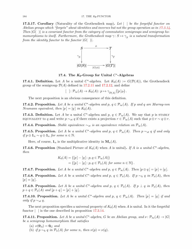
184 17. THE K0-FUNCTOR
17.3.17. Corollary (Naturality of the Grothendieck map). Let | | be the forgetful functor onAbelian groups which “forgets” about identities and inverses but not the group operation as in 17.3.14.Then |G( )| is a covariant functor from the category of commutative semigroups and semigroup ho-momorphisms to itself. Furthermore, the Grothendieck map γ : S 7→ γ
Sis a natural transformation
from the identity functor to the functor |G( )|.
|G(S)| |G(T )||G(φ)|
//
S
|G(S)|
γS
S Tφ // T
|G(T )|
γT
17.4. The K0-Group for Unital C∗-Algebras
17.4.1. Definition. Let A be a unital C∗-algebra. Let K0(A) := G(D(A)), the Grothendieckgroup of the semigroup D(A) defined in 17.2.11 and 17.2.12, and define
[ ] : P∞(A)→ K0(A) : p 7→ γD(A)
([p ]D
).
The next proposition is an obvious consequence of this definition.
17.4.2. Proposition. Let A be a unital C∗-algebra and p, q ∈ P∞(A). If p and q are Murray-vonNeumann equivalent, then [p ] = [q ] in K0(A).
17.4.3. Definition. Let A be a unital C∗-algebra and p, q ∈ P∞(A). We say that p is stablyequivalent to q and write p ∼st q if there exists a projection r ∈ P∞(A) such that p⊕ r ∼ q ⊕ r.
17.4.4. Proposition. Stable equivalence ∼st is an equivalence relation on P∞(A).
17.4.5. Proposition. Let A be a unital C∗-algebra and p, q ∈ P∞(A). Then p ∼st q if and onlyif p⊕ 1n ∼ q ⊕ 1n for some n ∈ N.
Here, of course, 1n is the multiplicative identity in Mn(A).
17.4.6. Proposition (Standard Picture of K0(A) when A is unital). If A is a unital C∗-algebra,then
K0(A) = [p ]− [q ] : p, q ∈ P∞(A)= [p ]− [q ] : p, q ∈ Pn(A) for some n ∈ N .
17.4.7. Proposition. Let A be a unital C∗-algebra and p, q ∈ P∞(A). Then [p⊕ q ] = [p ] + [q ].
17.4.8. Proposition. Let A be a unital C∗-algebra and p, q ∈ Pn(A). If p ∼h q in Pn(A), then[p ] = [q ].
17.4.9. Proposition. Let A be a unital C∗-algebra and p, q ∈ Pn(A). If p ⊥ q in Pn(A), thenp+ q ∈ Pn(A) and [p+ q ] = [p ] + [q ].
17.4.10. Proposition. Let A be a unital C∗-algebra and p, q ∈ P∞(A). Then [p ] = [q ] if andonly if p ∼st q.
The next proposition specifies a universal property of K0(A) when A is unital. In it the forgetfulfunctor | | is the one described in proposition 17.3.14.
17.4.11. Proposition. Let A be a unital C∗-algebra, G be an Abelian group, and ν : P∞(A)→ |G|be a semigroup homomorphism that satisfies
(a) ν(0A) = 0G and(b) if p ∼h q in Pn(A) for some n, then ν(p) = ν(q).
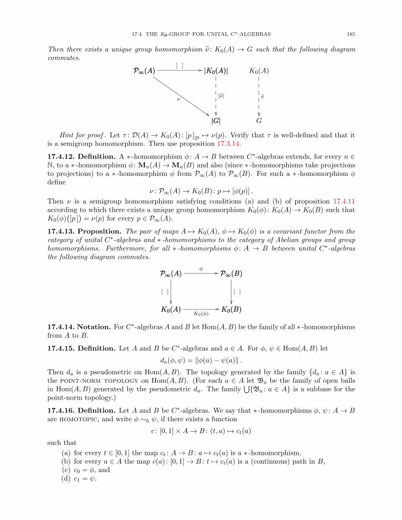
17.4. THE K0-GROUP FOR UNITAL C∗-ALGEBRAS 185
Then there exists a unique group homomorphism ν : K0(A) → G such that the following diagramcommutes.
P∞(A) |K0(A)|[ ] //P∞(A)
|G|
ν
$$
|K0(A)|
|G|
|ν|
K0(A)
G
ν
Hint for proof . Let τ : D(A) → K0(A) : [p ]D 7→ ν(p). Verify that τ is well-defined and that itis a semigroup homomorphism. Then use proposition 17.3.14.
17.4.12. Definition. A ∗ -homomorphism φ : A→ B between C∗-algebras extends, for every n ∈N, to a ∗ -homomorphism φ : Mn(A)→Mn(B) and also (since ∗ -homomorphisms take projectionsto projections) to a ∗ -homomorphism φ from P∞(A) to P∞(B). For such a ∗ -homomorphism φdefine
ν : P∞(A)→ K0(B) : p 7→ [φ(p)] .
Then ν is a semigroup homomorphism satisfying conditions (a) and (b) of proposition 17.4.11according to which there exists a unique group homomorphism K0(φ) : K0(A)→ K0(B) such thatK0(φ)
([p ])
= ν(p) for every p ∈ P∞(A).
17.4.13. Proposition. The pair of maps A 7→ K0(A), φ 7→ K0(φ) is a covariant functor from thecategory of unital C∗-algebras and ∗ -homomorphisms to the category of Abelian groups and grouphomomorphisms. Furthermore, for all ∗ -homomorphisms φ : A → B between unital C∗-algebrasthe following diagram commutes.
K0(A) K0(B)K0(φ)
//
P∞(A)
K0(A)
[ ]
P∞(A) P∞(B)φ // P∞(B)
K0(B)
[ ]
17.4.14. Notation. For C∗-algebras A and B let Hom(A,B) be the family of all ∗ -homomorphismsfrom A to B.
17.4.15. Definition. Let A and B be C∗-algebras and a ∈ A. For φ, ψ ∈ Hom(A,B) let
da(φ, ψ) = ‖φ(a)− ψ(a)‖ .Then da is a pseudometric on Hom(A,B). The topology generated by the family da : a ∈ A isthe point-norm topology on Hom(A,B). (For each a ∈ A let Ba be the family of open ballsin Hom(A,B) generated by the pseudometric da. The family
⋃Ba : a ∈ A is a subbase for the
point-norm topology.)
17.4.16. Definition. Let A and B be C∗-algebras. We say that ∗ -homomorphisms φ, ψ : A→ Bare homotopic, and write φ ∼h ψ, if there exists a function
c : [0, 1]×A→ B : (t, a) 7→ ct(a)
such that
(a) for every t ∈ [0, 1] the map ct : A→ B : a 7→ ct(a) is a ∗ -homomorphism,(b) for every a ∈ A the map c(a) : [0, 1]→ B : t 7→ ct(a) is a (continuous) path in B,(c) c0 = φ, and(d) c1 = ψ.
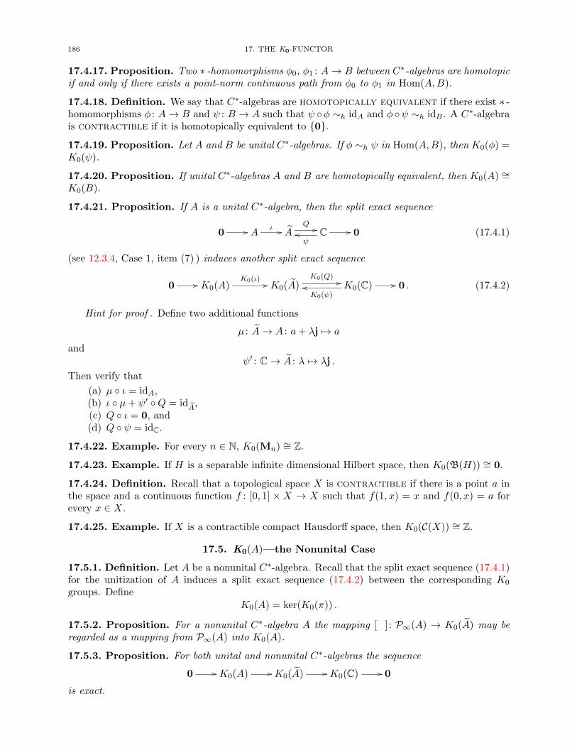
186 17. THE K0-FUNCTOR
17.4.17. Proposition. Two ∗ -homomorphisms φ0, φ1 : A→ B between C∗-algebras are homotopicif and only if there exists a point-norm continuous path from φ0 to φ1 in Hom(A,B).
17.4.18. Definition. We say that C∗-algebras are homotopically equivalent if there exist ∗ -homomorphisms φ : A→ B and ψ : B → A such that ψ φ ∼h idA and φ ψ ∼h idB. A C∗-algebrais contractible if it is homotopically equivalent to 0.
17.4.19. Proposition. Let A and B be unital C∗-algebras. If φ ∼h ψ in Hom(A,B), then K0(φ) =K0(ψ).
17.4.20. Proposition. If unital C∗-algebras A and B are homotopically equivalent, then K0(A) ∼=K0(B).
17.4.21. Proposition. If A is a unital C∗-algebra, then the split exact sequence
0 // Aι // A
Q //ooψ
C // 0 (17.4.1)
(see 12.3.4, Case 1, item (7) ) induces another split exact sequence
0 // K0(A)K0(ι) // K0(A)
K0(Q) //ooK0(ψ)
K0(C) // 0 . (17.4.2)
Hint for proof . Define two additional functions
µ : A→ A : a+ λj 7→ a
andψ′ : C→ A : λ 7→ λj .
Then verify that
(a) µ ι = idA,(b) ι µ+ ψ′ Q = id
A,
(c) Q ι = 0, and(d) Q ψ = idC.
17.4.22. Example. For every n ∈ N, K0(Mn) ∼= Z.
17.4.23. Example. If H is a separable infinite dimensional Hilbert space, then K0(B(H)) ∼= 0.
17.4.24. Definition. Recall that a topological space X is contractible if there is a point a inthe space and a continuous function f : [0, 1] ×X → X such that f(1, x) = x and f(0, x) = a forevery x ∈ X.
17.4.25. Example. If X is a contractible compact Hausdorff space, then K0(C(X)) ∼= Z.
17.5. K0(A)—the Nonunital Case
17.5.1. Definition. Let A be a nonunital C∗-algebra. Recall that the split exact sequence (17.4.1)for the unitization of A induces a split exact sequence (17.4.2) between the corresponding K0
groups. DefineK0(A) = ker(K0(π)) .
17.5.2. Proposition. For a nonunital C∗-algebra A the mapping [ ] : P∞(A) → K0(A) may beregarded as a mapping from P∞(A) into K0(A).
17.5.3. Proposition. For both unital and nonunital C∗-algebras the sequence
0 // K0(A) // K0(A) // K0(C) // 0
is exact.
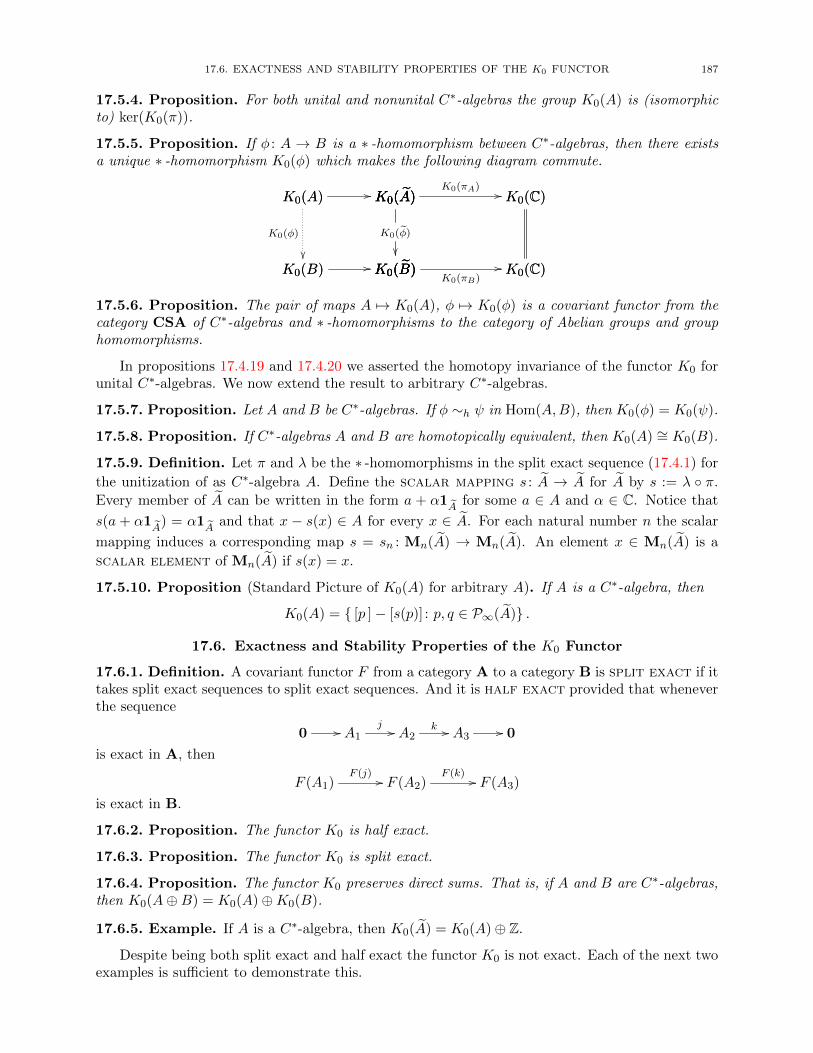
17.6. EXACTNESS AND STABILITY PROPERTIES OF THE K0 FUNCTOR 187
17.5.4. Proposition. For both unital and nonunital C∗-algebras the group K0(A) is (isomorphicto) ker(K0(π)).
17.5.5. Proposition. If φ : A → B is a ∗ -homomorphism between C∗-algebras, then there existsa unique ∗ -homomorphism K0(φ) which makes the following diagram commute.
K0(B) K0(B)//
K0(A)
K0(B)
K0(φ)
K0(A) K0(A)// K0(A)
K0(B)
K0(φ)
K0(B) K0(C)K0(πB)
//
K0(A)
K0(B)
K0(A) K0(C)K0(πA) // K0(C)
K0(C)
17.5.6. Proposition. The pair of maps A 7→ K0(A), φ 7→ K0(φ) is a covariant functor from thecategory CSA of C∗-algebras and ∗ -homomorphisms to the category of Abelian groups and grouphomomorphisms.
In propositions 17.4.19 and 17.4.20 we asserted the homotopy invariance of the functor K0 forunital C∗-algebras. We now extend the result to arbitrary C∗-algebras.
17.5.7. Proposition. Let A and B be C∗-algebras. If φ ∼h ψ in Hom(A,B), then K0(φ) = K0(ψ).
17.5.8. Proposition. If C∗-algebras A and B are homotopically equivalent, then K0(A) ∼= K0(B).
17.5.9. Definition. Let π and λ be the ∗ -homomorphisms in the split exact sequence (17.4.1) for
the unitization of as C∗-algebra A. Define the scalar mapping s : A → A for A by s := λ π.
Every member of A can be written in the form a + α1A
for some a ∈ A and α ∈ C. Notice that
s(a + α1A
) = α1A
and that x − s(x) ∈ A for every x ∈ A. For each natural number n the scalar
mapping induces a corresponding map s = sn : Mn(A) → Mn(A). An element x ∈ Mn(A) is a
scalar element of Mn(A) if s(x) = x.
17.5.10. Proposition (Standard Picture of K0(A) for arbitrary A). If A is a C∗-algebra, then
K0(A) = [p ]− [s(p)] : p, q ∈ P∞(A) .
17.6. Exactness and Stability Properties of the K0 Functor
17.6.1. Definition. A covariant functor F from a category A to a category B is split exact if ittakes split exact sequences to split exact sequences. And it is half exact provided that wheneverthe sequence
0 // A1j // A2
k // A3// 0
is exact in A, then
F (A1)F (j) // F (A2)
F (k) // F (A3)
is exact in B.
17.6.2. Proposition. The functor K0 is half exact.
17.6.3. Proposition. The functor K0 is split exact.
17.6.4. Proposition. The functor K0 preserves direct sums. That is, if A and B are C∗-algebras,then K0(A⊕B) = K0(A)⊕K0(B).
17.6.5. Example. If A is a C∗-algebra, then K0(A) = K0(A)⊕ Z.
Despite being both split exact and half exact the functor K0 is not exact. Each of the next twoexamples is sufficient to demonstrate this.
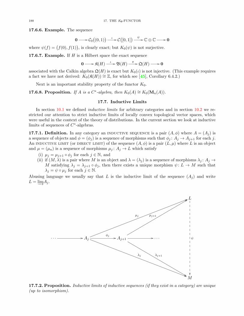
188 17. THE K0-FUNCTOR
17.6.6. Example. The sequence
0 // C0
((0, 1)
) ι // C([0, 1]
) ψ // C⊕ C // 0
where ψ(f) =(f(0), f(1)
), is clearly exact; but K0(ψ) is not surjective.
17.6.7. Example. If H is a Hilbert space the exact sequence
0 // K(H)ι // B(H)
π // Q(H) // 0
associated with the Calkin algebra Q(H) is exact but K0(ι) is not injective. (This example requiresa fact we have not derived: K0(K(H)) ∼= Z, for which see [45], Corollary 6.4.2.)
Next is an important stability property of the functor K0.
17.6.8. Proposition. If A is a C∗-algebra, then K0(A) ∼= K0(Mn(A)).
17.7. Inductive Limits
In section 10.1 we defined inductive limits for arbitrary categories and in section 10.2 we re-stricted our attention to strict inductive limits of locally convex topological vector spaces, whichwere useful in the context of the theory of distributions. In the current section we look at inductivelimits of sequences of C∗-algebras.
17.7.1. Definition. In any category an inductive sequence is a pair (A, φ) where A = (Aj) isa sequence of objects and φ = (φj) is a sequence of morphisms such that φj : Aj → Aj+1 for each j.An inductive limit (or direct limit) of the sequence (A, φ) is a pair (L, µ) where L is an objectand µ = (µn) is a sequence of morphisms µj : Aj → L which satisfy
(i) µj = µj+1 φj for each j ∈ N, and(ii) if (M,λ) is a pair where M is an object and λ = (λj) is a sequence of morphisms λj : Aj →
M satisfying λj = λj+1 φj , then there exists a unique morphism ψ : L → M such thatλj = ψ µj for each j ∈ N.
Abusing language we usually say that L is the inductive limit of the sequence (Aj) and writeL = lim−→Aj .
L
ψ
· · · // Aj
µj
55
λj
))
φj // Aj+1
µj+1
88
λj+1
&&
// · · ·
M
17.7.2. Proposition. Inductive limits of inductive sequences (if they exist in a category) are unique(up to isomorphism).
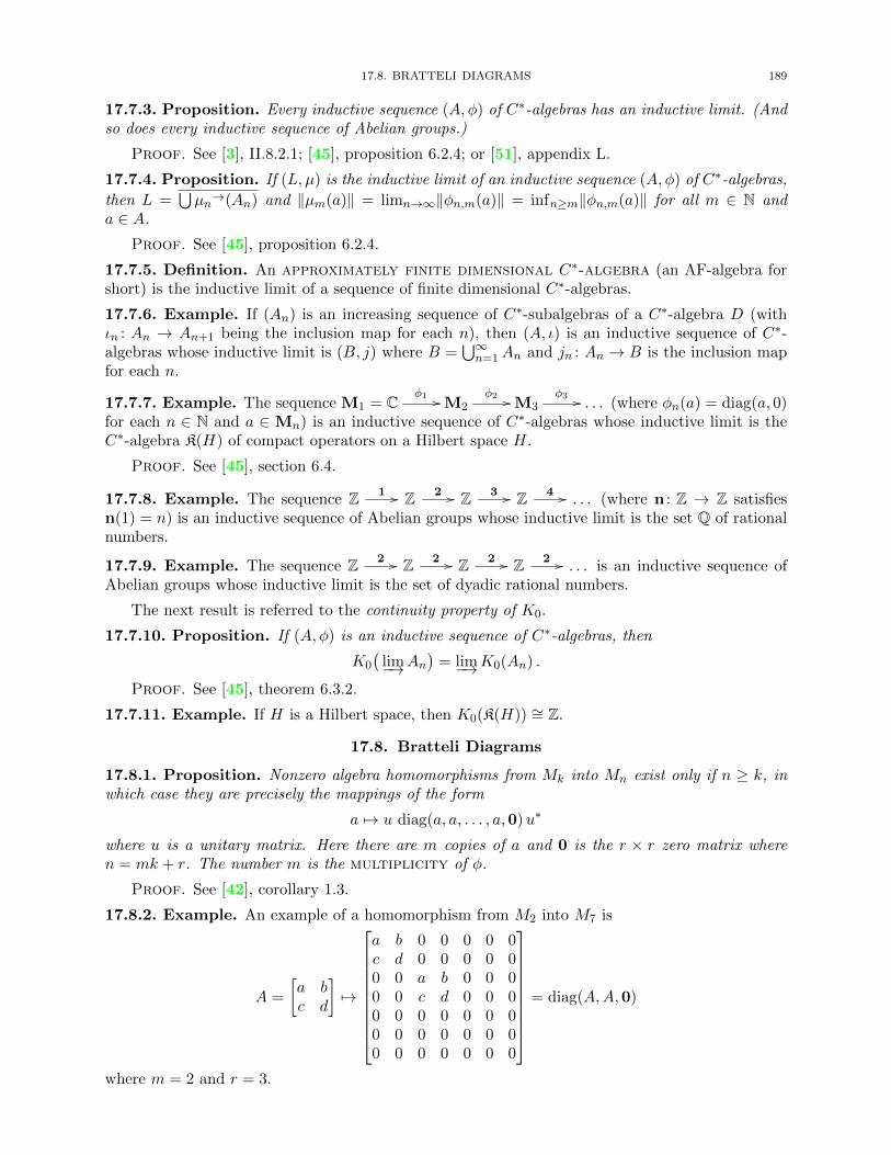
17.8. BRATTELI DIAGRAMS 189
17.7.3. Proposition. Every inductive sequence (A, φ) of C∗-algebras has an inductive limit. (Andso does every inductive sequence of Abelian groups.)
Proof. See [3], II.8.2.1; [45], proposition 6.2.4; or [51], appendix L.
17.7.4. Proposition. If (L, µ) is the inductive limit of an inductive sequence (A, φ) of C∗-algebras,
then L =⋃µn→(An) and ‖µm(a)‖ = limn→∞‖φn,m(a)‖ = infn≥m‖φn,m(a)‖ for all m ∈ N and
a ∈ A.
Proof. See [45], proposition 6.2.4.
17.7.5. Definition. An approximately finite dimensional C∗-algebra (an AF-algebra forshort) is the inductive limit of a sequence of finite dimensional C∗-algebras.
17.7.6. Example. If (An) is an increasing sequence of C∗-subalgebras of a C∗-algebra D (withιn : An → An+1 being the inclusion map for each n), then (A, ι) is an inductive sequence of C∗-algebras whose inductive limit is (B, j) where B =
⋃∞n=1An and jn : An → B is the inclusion map
for each n.
17.7.7. Example. The sequence M1 = Cφ1 //M2
φ2 //M3φ3 // . . . (where φn(a) = diag(a, 0)
for each n ∈ N and a ∈ Mn) is an inductive sequence of C∗-algebras whose inductive limit is theC∗-algebra K(H) of compact operators on a Hilbert space H.
Proof. See [45], section 6.4.
17.7.8. Example. The sequence Z 1 // Z 2 // Z 3 // Z 4 // . . . (where n : Z → Z satisfiesn(1) = n) is an inductive sequence of Abelian groups whose inductive limit is the set Q of rationalnumbers.
17.7.9. Example. The sequence Z 2 // Z 2 // Z 2 // Z 2 // . . . is an inductive sequence ofAbelian groups whose inductive limit is the set of dyadic rational numbers.
The next result is referred to the continuity property of K0.
17.7.10. Proposition. If (A, φ) is an inductive sequence of C∗-algebras, then
K0
(lim−→An
)= lim−→K0(An) .
Proof. See [45], theorem 6.3.2.
17.7.11. Example. If H is a Hilbert space, then K0(K(H)) ∼= Z.
17.8. Bratteli Diagrams
17.8.1. Proposition. Nonzero algebra homomorphisms from Mk into Mn exist only if n ≥ k, inwhich case they are precisely the mappings of the form
a 7→ u diag(a, a, . . . , a,0)u∗
where u is a unitary matrix. Here there are m copies of a and 0 is the r × r zero matrix wheren = mk + r. The number m is the multiplicity of φ.
Proof. See [42], corollary 1.3.
17.8.2. Example. An example of a homomorphism from M2 into M7 is
A =
[a bc d
]7→
a b 0 0 0 0 0c d 0 0 0 0 00 0 a b 0 0 00 0 c d 0 0 00 0 0 0 0 0 00 0 0 0 0 0 00 0 0 0 0 0 0
= diag(A,A,0)
where m = 2 and r = 3.
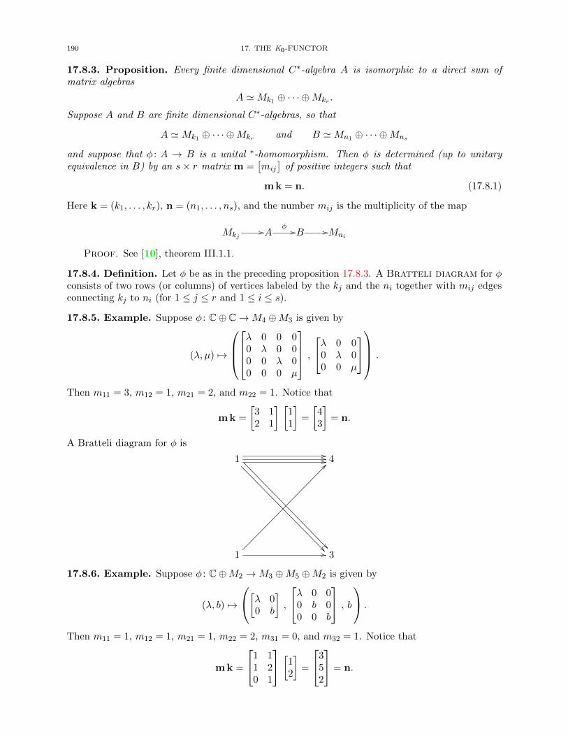
190 17. THE K0-FUNCTOR
17.8.3. Proposition. Every finite dimensional C∗-algebra A is isomorphic to a direct sum ofmatrix algebras
A 'Mk1 ⊕ · · · ⊕Mkr .
Suppose A and B are finite dimensional C∗-algebras, so that
A 'Mk1 ⊕ · · · ⊕Mkr and B 'Mn1 ⊕ · · · ⊕Mns
and suppose that φ : A → B is a unital ∗-homomorphism. Then φ is determined (up to unitaryequivalence in B) by an s× r matrix m =
[mij
]of positive integers such that
m k = n. (17.8.1)
Here k = (k1, . . . , kr), n = (n1, . . . , ns), and the number mij is the multiplicity of the map
Mkj//A
φ //B //Mni
Proof. See [10], theorem III.1.1.
17.8.4. Definition. Let φ be as in the preceding proposition 17.8.3. A Bratteli diagram for φconsists of two rows (or columns) of vertices labeled by the kj and the ni together with mij edgesconnecting kj to ni (for 1 ≤ j ≤ r and 1 ≤ i ≤ s).
17.8.5. Example. Suppose φ : C⊕ C→M4 ⊕M3 is given by
(λ, µ) 7→
λ 0 0 00 λ 0 00 0 λ 00 0 0 µ
,λ 0 0
0 λ 00 0 µ
.
Then m11 = 3, m12 = 1, m21 = 2, and m22 = 1. Notice that
m k =
[3 12 1
] [11
]=
[43
]= n.
A Bratteli diagram for φ is
1//////
4
1
??
// 3
17.8.6. Example. Suppose φ : C⊕M2 →M3 ⊕M5 ⊕M2 is given by
(λ, b) 7→
[λ 00 b
],
λ 0 00 b 00 0 b
, b .
Then m11 = 1, m12 = 1, m21 = 1, m22 = 2, m31 = 0, and m32 = 1. Notice that
m k =
1 11 20 1
[12
]=
352
= n.
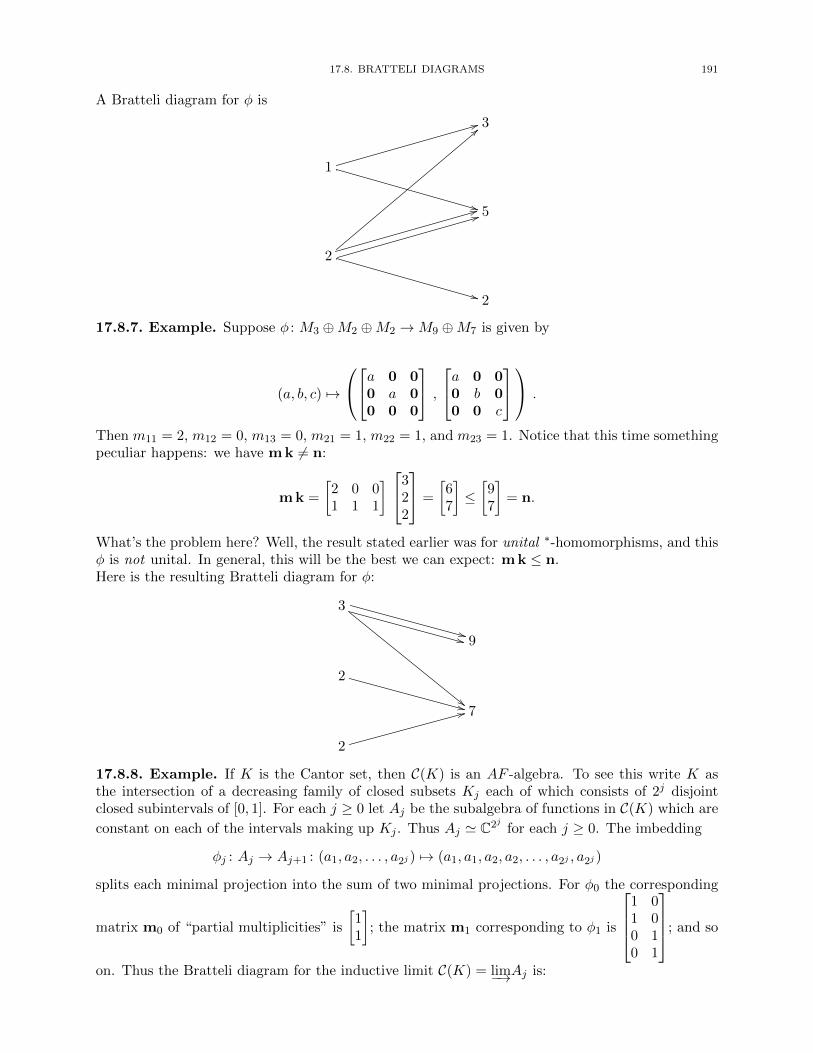
17.8. BRATTELI DIAGRAMS 191
A Bratteli diagram for φ is
3
1
44
** 5
2
==
44 44
** 2
17.8.7. Example. Suppose φ : M3 ⊕M2 ⊕M2 →M9 ⊕M7 is given by
(a, b, c) 7→
a 0 00 a 00 0 0
,a 0 0
0 b 00 0 c
.
Then m11 = 2, m12 = 0, m13 = 0, m21 = 1, m22 = 1, and m23 = 1. Notice that this time somethingpeculiar happens: we have m k 6= n:
m k =
[2 0 01 1 1
] 322
=
[67
]≤[97
]= n.
What’s the problem here? Well, the result stated earlier was for unital ∗-homomorphisms, and thisφ is not unital. In general, this will be the best we can expect: m k ≤ n.Here is the resulting Bratteli diagram for φ:
3
++++
""
9
2
++ 7
2
33
17.8.8. Example. If K is the Cantor set, then C(K) is an AF -algebra. To see this write K asthe intersection of a decreasing family of closed subsets Kj each of which consists of 2j disjointclosed subintervals of [0, 1]. For each j ≥ 0 let Aj be the subalgebra of functions in C(K) which are
constant on each of the intervals making up Kj . Thus Aj ' C2j for each j ≥ 0. The imbedding
φj : Aj → Aj+1 : (a1, a2, . . . , a2j ) 7→ (a1, a1, a2, a2, . . . , a2j , a2j )
splits each minimal projection into the sum of two minimal projections. For φ0 the corresponding
matrix m0 of “partial multiplicities” is
[11
]; the matrix m1 corresponding to φ1 is
1 01 00 10 1
; and so
on. Thus the Bratteli diagram for the inductive limit C(K) = lim−→Aj is:
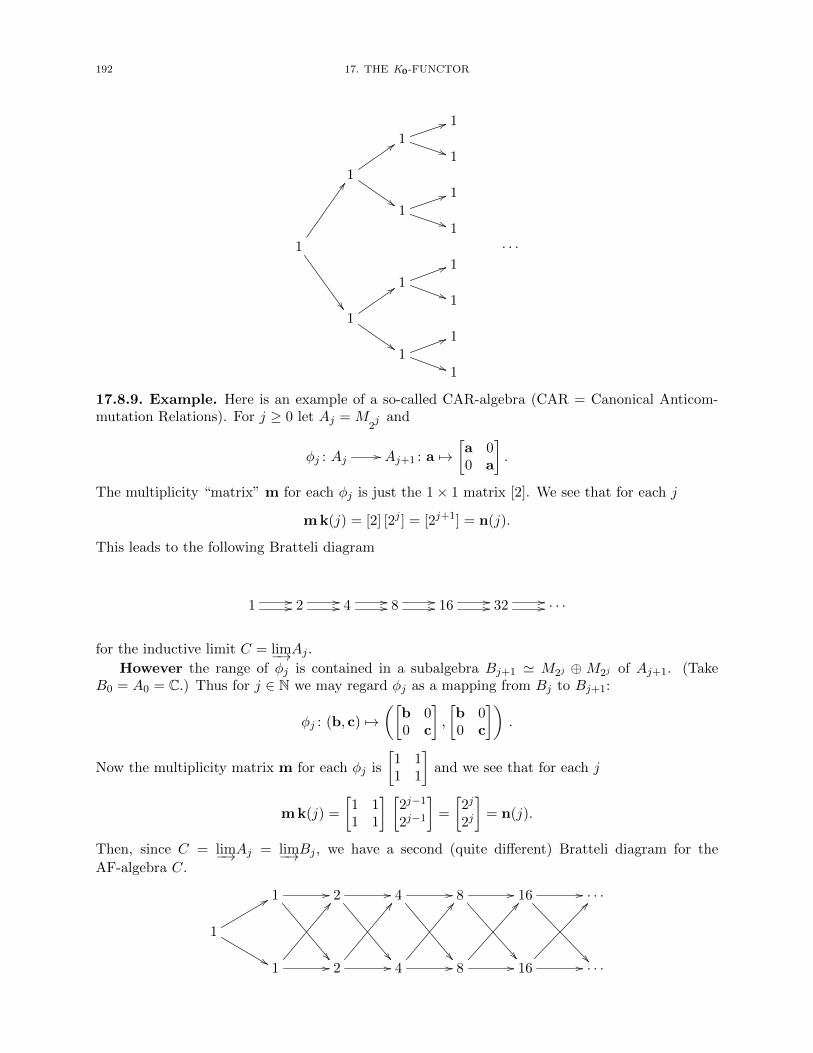
192 17. THE K0-FUNCTOR
11
55
)) 11
::
$$1
1
55
)) 11
DD
· · ·1
1
55
)) 11
::
$$1
1
55
)) 1
17.8.9. Example. Here is an example of a so-called CAR-algebra (CAR = Canonical Anticom-mutation Relations). For j ≥ 0 let Aj = M
2j and
φj : Aj // Aj+1 : a 7→[a 00 a
].
The multiplicity “matrix” m for each φj is just the 1× 1 matrix [2]. We see that for each j
m k(j) = [2] [2j ] = [2j+1] = n(j).
This leads to the following Bratteli diagram
1 //// 2 //// 4 //// 8 //// 16 //// 32 //// · · ·
for the inductive limit C = lim−→Aj .However the range of φj is contained in a subalgebra Bj+1 ' M2j ⊕ M2j of Aj+1. (Take
B0 = A0 = C.) Thus for j ∈ N we may regard φj as a mapping from Bj to Bj+1:
φj : (b, c) 7→([
b 00 c
],
[b 00 c
]).
Now the multiplicity matrix m for each φj is
[1 11 1
]and we see that for each j
m k(j) =
[1 11 1
] [2j−1
2j−1
]=
[2j
2j
]= n(j).
Then, since C = lim−→Aj = lim−→Bj , we have a second (quite different) Bratteli diagram for the
AF-algebra C.
1 //
2 //
4 //
8 //
16 //
· · ·
1
88
&&1 //
BB
2 //
BB
4 //
BB
8 //
AA
16 //
@@
· · ·
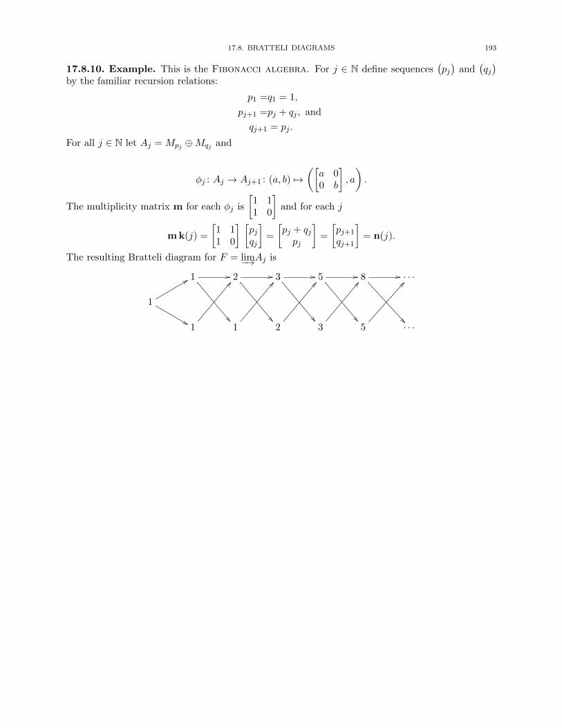
17.8. BRATTELI DIAGRAMS 193
17.8.10. Example. This is the Fibonacci algebra. For j ∈ N define sequences(pj)
and(qj)
by the familiar recursion relations:
p1 =q1 = 1,
pj+1 =pj + qj , and
qj+1 = pj .
For all j ∈ N let Aj = Mpj ⊕Mqj and
φj : Aj → Aj+1 : (a, b) 7→([a 00 b
], a
).
The multiplicity matrix m for each φj is
[1 11 0
]and for each j
m k(j) =
[1 11 0
] [pjqj
]=
[pj + qjpj
]=
[pj+1
qj+1
]= n(j).
The resulting Bratteli diagram for F = lim−→Aj is
1 //
2 //
3 //
5 //
8 //
· · ·
1
88
&&1
BB
1
BB
2
BB
3
BB
5
@@
· · ·

Bibliography
1. William Arveson, A Short Course on Spectral Theory, Springer-Verlag, New York, 2002. 161, 166, 167, 1682. Larry Baggett and Watson Fulks, Fourier Analysis, Anjou Press, Boulder, Colorado, 1979. 130, 1313. Bruce Blackadar, Operator Algebras: Theory of C∗-algebras and von Neumann Algebras, Springer-Verlag, Berlin,
2006. 137, 149, 161, 175, 1894. A. L. Brown and A. Page, Elements of Functional Analysis, Van Nostrand Reinhold, London, 1970. 27, 72, 775. Arlen Brown and Carl Pearcy, Introduction to Operator Theory I: Elements of Functional Analysis, Springer-
Verlag, New York, 1977. 736. L. G. Brown, R. G. Douglas, and P. A. Fillmore, Unitary Equivalence Modulo the Compact Operators and
Extensions of C∗-algebras, Springer-Verlag, Lecture Notes in Mathematics 345 (1973), 58–128. ix7. Joan Cerda, Linear Functional Analysis, American Mathematicasl Society, Providence, Rhode Island, 2010. 1228. John B. Conway, A Course in Functional Analysis, second ed., Springer-Verlag, New York, 1990. 27, 41, 82, 92,
100, 109, 115, 149, 157, 1609. , A Course in Operator Theory, American Mathematical Society, Providence, Rhode Island, 2000. 41, 165
10. Kenneth R. Davidson, C*-Algebras by Example, American Mathematical Society, Providence, R.I., 1996. 92, 137,146, 165, 166, 167, 168, 169, 190
11. Robert S. Doran and Victor A. Belfi, Characterizations of C*-Algebras, Marcel Dekker, New York, 1986. 144, 14912. Ronald G. Douglas, Banach Algebra Techniques in Operator Theory, Academic Press, New York, 1972. 132, 161,
162, 166, 167, 16813. , C*-Algebra Extensions and K-Homology, Princeton University Press, Princeton, 1980. 17114. Per H. Enflo, A counterexample to the approximation problem in Banach spaces, Acta Mathematica 130, no. 1
(1973), 309–317. 9115. John M. Erdman, A ProblemText in Advanced Calculus,
http://web.pdx.edu/~erdman/PTAC/PTAClicensepage.html. x16. , A Companion to Real Analysis, 2007,
http://web.pdx.edu/~erdman/CRA/CRAlicensepage.html. x, 16, 27, 45, 49, 71, 73, 74, 97, 136, 14117. , Elements of Linear and Multilinear Algebra, 2010,
http://web.pdx.edu/~erdman/ELMA/ELMA_licensepage.html. x, 1, 318. Peter A. Fillmore, A User’s Guide to Operator Algebras, John Wiley and Sons, New York, 1996. 137, 146, 149,
17519. Gerald B. Folland, Real Analysis: Modern Techniques and their Applications, John Wiley and Sons, New York,
1984. 8220. Michael Frank, Hilbert C*-modules and related subjects—a guided reference overview, 2010,
http://www.imn.htwk-leipzig.de/~mfrank/mlit.pdf. 15421. Gerd Grubb, Distributions and Operators, Springer, New York, 2009. 115, 11722. Dzung Minh Ha, Functional Analysis: Volume 1:A Gentle Introduction, Matrix Editions, Ithaca, NY, 2006. 4123. Paul R. Halmos, Introduction to Hilbert Space, Chelsea, New York, 1951, 1957. 41, 4724. , A Hilbert Space Problem Book, second ed., Springer-Verlag, New York, 1982. ix, 58, 87, 16825. Gilbert Helmberg, Introduction to Spectral Theory in Hilbert Spasce, North Holland, Amsterdam, 1969. 4126. Edwin Hewitt and Karl Stromberg, Real and Abstract Analysis, Springer-Verlag, New York, 1965. 82, 119, 13027. Nigel Higson and John Roe, Analytic K-Homology, Oxford University Press, Oxford, 2000. 146, 161, 163, 165,
167, 168, 171, 172, 174, 17528. Francis Hirsch and Gilles Lacombe, Elements of Functional Analysis, Springer, New York, 1999. 11729. Harry Hochstadt, Eduard Helly, father of the Hahn-Banach theorem, The Masthematical Intelligencer 2, issue
3 (1980), 123–125. 3730. Kenneth Hoffman and Ray Kunze, Linear Algebra, second ed., Prentice Hall, Englewood Cliffs,N.J., 1971. 6, 7,
1431. John Horvath, Topological Vector Spaces and Distributions, Addison-Wesley, Reading, Massachusetts, 1966. 12232. Richard V. Kadison and John R. Ringrose, Fundamentals of the Theory of Operator Algebras, volumes I–IV,
Academic Press, New York, 1983. 92, 147, 14933. Erwin Kreyszig, Introductory Functional Analysis with Applications, John Wiley, New York, 1978. 27, 41, 47
195
196 BIBLIOGRAPHY
34. Saunders Mac Lane, Categories for the Working Mathematician, Springer Verlag, New York, 1971. 1535. F. William Lawvere and Stephen H. Schanuel, Conceptual Mathematics: A First Introduction to Categories,
Cambridge University Press, Cambridge, 1997. 1536. William S. Massey, Algebraic Topology: An Introduction, Harcourt, Brace, and World, New York, 1967, [Ma]. 16837. R. Daniel Mauldin (ed.), TheScottish Book: Mathematics from the Scottish Cafe, Birkhauser, Boston, 1981. 9138. John N. McDonald and Neil A. Weiss, A Course in Real Analysis, Academic Press, San Diego, 1999. 82, 12239. Gerard J. Murphy, C*-Algebras and Operator Theory, Academic Press, San Diego, 1990. 92, 137, 149, 166, 167,
168, 17540. Vern Paulsen, Completely Bounded Maps and Operator Algebras, Cambridge University Press, Cambridge, 2002.
174, 17541. Gert K. Pedersen, Analysis Now: Revised Printing, Springer-Verlag, New York, 1995. 73, 92, 162, 16342. Stephen C. Power, Limit Algebras: an Introduction to Subalgebras of C*-algebras, Longman Scientific and Tech-
nical, Harlow, Essex, 1992. 18943. Iain Raeburn and Dana P. Williams, Morita Equivalence and Continuous-Trace C*-Algebras, American Mathe-
matical Society, Providence, R.I., 1998. 15444. Steven Roman, Advanced Linear Algebra, second ed., Springer, New York, 2005. 1445. M. Rørdam, F. Larsen, and N. J. Laustsen, An Introduction to K-Theory for C*-Algebras, Cambridge University
Press, Cambridge, 2000. 177, 179, 188, 18946. Walter Rudin, Real and Complex Analysis, third ed., McGraw-Hill, New York, 1987. 82, 9847. , Functional Analysis, second ed., McGraw-Hill, New York, 1991. 27, 109, 110, 117, 118, 119, 120, 121,
122, 12348. Zbigniew Semadeni, Banach Spaces of Continuous Functions, Polish Scientific Publishers, Warzawa, 1971. 15,
12849. Francois Treves, Topological Vector Spaces, Distributions and Kernels, Academic Press, New York, 1967. 110,
111, 115, 12250. Andrew H. Wallace, Algebraic Topology: Homology and Cohomology, W. A. Benjamin, New York, 1970. 16851. N. E. Wegge-Olsen, K-Theory and C*-Algebras, Oxford University Press, Oxford, 1993. 137, 161, 162, 163, 175,
177, 18952. Wikipedia, Wikipedia, The Free Encyclopedia, http://en.wikipedia.org. 5153. Stephen Willard, General Topology, Addison-Wesley, Reading, Mass., 1968. 157, 16854. Kosaku Yosida, Functional Analysis, Academic Press/Springer-Verlag, New York/Berlin, 1965. 117, 12255. Nicholas Young, An Introduction to Hilbert Space, Cambridge University Press, Cambridge, 1988. 41
Index
χA
(characteristic function of A), 52f |A (restriction of f to A), xiv∐Aλ (coproduct), 33∏Sλ (Cartesian product), 30
Aop (opposite algebra of A), 151AB (in algebras the span of products of elements),
155f←(B) (inverse image of set B under function f), xivfn ↓ g (ptws) (pointwise monotone convergence), 22fn ↑ g (ptws) (pointwise monotone convergence), 22
fλw∗ // g (weak star convergence), 72
xλw // a (weak convergence), 72
Sα // T (morphism in a category), 16
B→ a (convergence of a filterbase), 104lim−→Ai (inductive limit), 113
f→(A) (image of set A under function f), xivfn → g (ptws) (pointwise convergence), 22fn → g (unif) (uniform convergence), 22xλ → a (convergence of nets), 34
xnw // a (weak sequential convergence), 86
Tλ → S, 87
TλSOT // S, 87
TλWOT // S, 87
V/M (quotient of V by M), 28[p ]D + [q ]D (addition in D(A)), 182a b (operation in an algebra), 142f ∗ g (convolution of two functions), 119u ∗ φ (convolution of a distribution and a test
function), 119u ∗ v (convolution of two distributions), 120βα (notation for composition of morphisms), 16fu (product of a smooth function with a
distribution), 118 (direct difference), 65⊕ (direct sum), 30, 31⊕ (orthogonal direct sum), 11⊕ (vector space direct sum), 3A⊕B (direct sum of C∗-algebras), 138a⊕ b (an element of A⊕B), 138],
⊎(disjoint union), 33
A ./ C (unitization of an algebra), 135X ≈ Y (X and Y are homeomorphic), 127
U⊆ X (U is an open subset of X), 16
p g q (supremum of projections), 65p f q (infimum of projections), 65
p ⊥ q (orthogonality of projections), 64(a, b) ∼ (c, d) (Grothendieck equivalence), 182p ∼ q (Murray-von Neumann equivalence), 178, 181φ ∼h ψ (homotopy of ∗ -homomorphisms), 185p ∼h q (homotopy of points), 163a ∼s b (similarity of elements of an algebra), 177p ∼st q (stable equivalence), 184a ∼u b (unitary equivalence), 177
A ≺ B (A ⊆ B), 1104 (subspace of a Banach or Hilbert space), 44, 76f 4 g (g is an extension of f), 37p q (ordering of projections in a ∗ -algebra), 65x ⊥ y (orthogonal vectors), 10[T, T ∗] (commutator of T ), 165〈x | y〉 (inner product), 151〈a, b〉 (pair in Grothendieck construction), 182〈x, y〉 (inner product), 8[a, b] (closed segment in a vector space), 23[p ] (image under the Grothendieck map of [p ]D), 184[x] (equivalence class containing x), 28[p]D (∼ equivalence class of p), 181
V + (positive cone in an ordered vector space), 143kerT (kernel of T ), 4< (notation for a strict ordering), 16≤ (notation for a partial ordering), 16
A⊥ (annihilator of a set), 82A+ (positive cone), 143c+ (positive part of c), 144c− (negative part of c), 144ranT (range of T ), 4≤ (notation for a partial ordering), 143a ≤ b (order relation in a C∗-algebra), 143g . f (relation between operator valued maps), 174s(x, y) (semi-inner product), 8∗ -algebra, 62
quotient, 67∗ -homomorphism, 62
homotopy of, 185unital, 62∗ -ideal, 67∗ -isomorphism, 62∗ -subalgebra (self-adjoint subalgebra), 63∑A (sum of a set of vectors), 42∑i∈I xi (sum of an indexed family), 42
p⊕ q (binary operation in P∞(A)), 181
J⊥ (annihilator of J), 155f←(B) (preimage of B under f), 16
197
198 INDEX
f→(A) or f(A) (image of A under f), 16Ae (unitization of a Banach algebra), 135(V )r (open ball of radius r about the origin), 73|A| (the forgetful functor acting on A), 19|A| (underlying set of the object A), 17|a| (absolute value in a C∗-algebra), 144‖T‖ (norm of a bounded linear map T ), 26‖x‖ (norm of a vector x), 10‖ ‖cb (norm of completely bounded map), 174‖ ‖1 (1-norm), 21, 25, 31, 119‖ ‖2 (Euclidean norm or 2-norm), 31‖ ‖∞ (uniform norm), 21, 25‖ ‖u (uniform norm), 21, 31∨A (closed linear span of A), 44
f (Fourier transform of f), 119u (Fourier transform of u), 123
f (regular distribution associated with f), 116a (Gelfand transform of a), 128
B 7→ B, T 7→ T (the functor), 79
A (closure of A), 37
A⊥ (orthogonal complement), 12
M⊥ (annihilator of a set), 71
T# (vector space adjoint), 20
V # (algebraic dual space), 12α−1 (inverse of a morphism α), 18A (interior of A), 37u′ (derivative of a distribution u), 116fα (multi-index notation for differentiation), 110uα (multi-index notation for differentiation), 117A∗ (set of complex conjugates of A ⊆ C), 99S∗ (set of adjoints of elements of S), 63T ∗ (Hilbert space adjoint), 59T ∗ (inner product space adjoint), 13T ∗ (normed linear space adjoint), 69V ∗ (dual space of a normed linear space), 26, 69τ? (conjugate of τ), 147F⊥ (pre-annihilator of a set), 71
AbGpthe category, 16
absolutecontinuity
of a function, 42convergence, 42value
in a C∗-algebra, 144absolutely
continuous, 42continuous functions
Hilbert space of, 42convergent
Fourier series, 130series, 25
summable, 42bilateral sequence, 126
AC(T) (absolutely convergent Fourier series, 130absorb, 103absorbing, 103abstract
spectral theorem, 132
Topelitzextension, 171operator, 171
abstract view of projections, 64addition
continuity of, 31on the Grothendieck group, 182
additiveinverses, 1
adjoint, 62, 153as a functor on HSp, 61formal, 121index of, 162inverse of an, 62of a linear map
between Hilbert spaces, 59between normed linear spaces, 69
of a multiplication operator, 60of an integral operator, 60of an inverse, 62of an operator on an inner product space, 13of the unilateral shift, 59vector space, 20
adjointable, 153AdU (conjugation by U), 169AF -algebraC(K) is an (K is the Cantor set), 191
AF-algebra, 189Alaoglu’s theorem, 72ALG
the category, 17algebra, 17, 151∗ -, 62C∗-, 90Banach, 41Calkin, 161commutative, 17homomorphism, 17
unital, 17multiplier, 157normed, 32opposite, 151quotient, 67
Banach, 77simple, 66Toeplitz, 167unital, 17unital normed, 32with involution, 62
algebraic∗-ideal, 137dual space, 12ideal, 137
A-linear, 153A-module, 151, 152
Hilbert, 153A as a, 153
inner product, 152morphism, 153pre-Hilbert, 152
INDEX 199
semi-inner product, 152analytic, 98annihilator, 71, 82, 155anti-isomorphism, 48, 151antihomomorphism, 151antisymmetric, 16approximate
identity, 145existence of an, 145sequential, 145
unit, 145approximate point spectrum, 100approximately finite dimensional C∗-algebra, 189arrow, 15associative, 1Atkinson’s theorem, 161A-valued (semi-)inner product, 152
Br(a), Br (open ball of radius r), 22Bp,ε, Bp (open semiball determined by p), 108B(S)
as a normed algebra, 32as a normed linear space, 21bounded functions on S, 21B(S, V )
as a normed linear space, 21Bounded V -valued functions on S, 21
B(V )as a C∗-algebra, 91as a unital algebra, 96as a unital Banach algebra, 90as a unital normed algebra, 32operators, 25
B(V,W )as a Banach space, 26as a normed linear space, 26bounded linear maps, 25
BA1
products in, 54BA∞
products in, 54balanced, 103
hull, 103BALG
products and coproducts in, 97quotients in, 77the category, 97
ballclosed, 22open, 22
BAN∞quotients in, 74the category, 78
BAN1
coproducts in, 54BAN∞
coproducts in, 53Banach
algebra, 41B(B) as a, 90coproduct, 97
direct sum, 97homomorphism, 97product, 97quotient, 77
space, 41C0(X) as a, 82L1(S, µ) as a, 42L1(R) as a, 118B(V,W ) as a, 26M(X) as a, 82c as a, 81c0 as a, 80l1 as a, 81quotient, 76
Banach-Steinhaus theorem, 86base
for a filter, 104for a topology, 24for neighborhoods of a point, 34local, 105
basicneighborhoods, 34open sets, 24
basisfor a Hilbert space, 46Hamel, 2orthonormal, 46Schauder, 81standard (or usual), 47, 81
Bessel’s inequality, 46bijective, xivbijective morphisms
are invertiblein ∗ -algebras, 62in BAN1, 74in CSA, 90in LAT, 18in SET, 18
need not be invertiblein POSET, 18
bilinear, 151Bohnenblust-Sobczyk-Suhomlinov theorem, 38bounded
away from zero, 61, 75below, 61, 75completely, 174in the weak operator topology, 87linear functionals, 26linear map, 25, 106
unitary, 165net in K, 36pointwise, 85sesquilinear functional, 58set in a TVS, 106totally, 89uniformly, 85weakly, 87
set in a normed linear space, 86boundedness
principle of uniform, 85
200 INDEX
Bratteli diagram, 190
Cr(a), Cr (closed ball of radius r), 22Cp,ε, Cp (closed semiball determined by p), 108C
as a C∗-algebra, 91field of complex numbers, 1
C (set of complex numbers), xiiiC (the functor), 20, 128C(X)
as a C∗-algebra, 91as a Banach space, 41as a unital algebra, 96as a vector space, 32continuous complex valued functions on X, 41C(X,R)
as a Banach space, 41continuous real valued functions on X, 41C([a, b])
as an inner product space, 9C∞(Ω)
infinitely differentiable functions, 110C∞c (Ω)
infinitely differentiable functions with compactsupport, 110
C0(X)as a C∗-algebra, 91as a Banach space, 82as a nonunital algebra, 96dual of, 82space of continuous functions which vanish at
infinity, 81Cb(X)
as a Banach space, 41as a normed algebra, 32as a normed linear space, 32continuous bounded functions on X, 32
cas a Banach space, 81as a normed linear space, 21convergent sequences, 21
c0as a Banach space, 80as a normed linear space, 21sequences which converge to zero, 21
C∗-algebra, 90L∞(S) as a, 91C as a, 91Mn(A) as a, 180C(X) as a, 91C0(X) as a, 91B(H) as a, 91L(V ) as a, 153direct sum of, 138generated by a set, 132Mn(A) as a, 172Mn as a, 91nuclear, 174
C∗-condition, 90C∗-embedding, 157C∗-norm, 90
C∗-subalgebra, 90C∗(S) (C∗-subalgebra generated by S), 132calculus
functional, 132Calkin algebra, 161cancellable
left, 18right, 18
cancellation property, 183CAR-algebras, 192Cartesian product, 30category, 15
ALG as a, 17AbGp as a, 16BALG as a, 97BAN∞ as a, 78CSA as a, 90HSp1 as a, 57HSp as a, 57LAT as a, 18NLS∞ as a, 25NLS1 as a, 27POSET as a, 16SET as a, 16TOP as a, 17TVS as a, 104VEC as a, 16concrete, 17geometric, 27, 57locally small, 16small, 16topological, 27, 57
C2 (pairs of objects and morphisms), 20Cauchy
filter, 107sequence, 27
weak, 86chain, 16character, 125
space, 126of C(X), 127of l1(Z), 126
characteristicfunction, 52
characterizationby nets
of interior, 37charactrization
by netsof closure, 37
chord, 58classical solution, 121closed, 16
ball, 22graph theorem, 75inverse, 146linear span, 44range
operator without, 59segment, 23
INDEX 201
semiball, 108weakly, 50
closure, 37characterization of by nets, 37
cluster pointof a net, 34
co(A) (convex hull of A), 23co-universal
morphism, 54Coburn’s theorem, 168codimension, 3, 48, 85, 160codomain, xivcokernel, 80, 160cokerT (the cokernel of T ), 80combination
convex, 23linear, 2
commutative, 2algebra, 17diagram, xiv
commutator, 165commute, xivcompact, 28
linear map, 90locally, 81relatively, 89weakly, 50
compactatopology of uniform convergence on, 105, 110
compactification, 156, 157essential, 156, 157
compalent, 165comparable, 16compatibility
of orderings with operations, 143compatible, 104complement
of a Banach subspace, 83of a vector subspace, 3orthogonal, 12
complemented subspace, 83complete
metric space, 27order, 19orthonormal set, 46product, 30topological vector space, 107weakly, 86
completelybounded, 174positive, 173
lifting property, 175completion
of a metric space, 55components
path, 163compression spectrum, 100concatenation, 52concrete category, 17cone, 93, 143
positive, 143proper, 93, 143
conjugatelinear, 8, 58
conjugate linear, 48conjugation, 48, 169connected
by a path, 163connecting morphisms, 113construction
Gelfand-Naimark-Segal, 148continuity
absoluteof a function, 42
characterization by nets, 36of K0, 189of addition, 31of norms, 22of scalar multiplication, 31uniform, 26
continuousfunction, 16linear functionals, 26weakly, 50, 89C(X)
as a nuclear C∗-algebra, 175continuously differentiable, 76contractibleC∗-algebras, 186topological space, 186
contractive, 27, 97contravariant functor, 19convention
basis for the zero vector space, 2conventionsA is a subset of A⊕B, 154about sesquilinear, 151about universality, 54all operators are bounded and linear, 25, 57ExtA consists of extensions or morphisms, 171essentially unique means unique up to
isomorphism, 30function = map = transformation, xivHilbert spaces are separable and infinite
dimensional (after section 9.2), 168ideals are closed, 137ideals are self-adjoint, 137ideals are two-sided, 66in an algebra AB denotes the span of products, 155in chapter 11 and those following scalars are
complex, 125in chapter 8 scalars are complex, 95notation for composition
of morphisms, 16on choice of product norm, 31on normed spaces strong topology refers to the
norm topology, 89projections in Hilbert spaces are orthogonal, 64representations of unital C∗-algebras are unital,
148
202 INDEX
subspaces of Banach spaces are closed, 76subspaces of Hilbert spaces are closed, 44subspaces of topological vector spaces are closed,
107vector spaces are complex or real, 1
convergenceabsolute, 42in Hilbert space
strong, 50weak, 50
in norm, 50of a filter, 104of a filterbase, 104of a series, 43of infinite series, 35, 42of nets, 34pointwise, 22uniform, 22
on compacta, 105, 110weak, 86
convergentabsolutely, 25series, 25
convexcombination, 23hull, 23locally, 108set, 23
convolutionin l1(Z), 126of a distribution and a test function, 119of functions in L1(R), 119of two distributions, 120
coordinateprojections, 30
coproduct, 33, 53in BALG, 97in BAN1, 54in BAN∞, 53in HIL, 53in SET, 33in VEC, 33in a category, 33uniqueness of, 33
correspondenceone-to-one, xiv
covariant functor, 19CSA
the category, 90CSA
products in, 138C∗-algebra
AF-algebras, 189CAR-algebras, 192Fibonacci algebra, 193inductive limit, 189
curve, 58cyclic
representation, 148vector, 148
Dα (multi-index notation for differentiation), 110,117
Du (derivative of a distribution u), 116D (open unit disk), xiiiD (closed unit disk in C), 103D(A) (set of equivalence classes of projections), 181D(Ω)
space of test functions; infinitely differentiablefunctions with compact support, 110
D∗(Ω) (space of distributions on Ω), 115d(x, y) (distance between points x and y), 10decomposition
Jordan, 144polar, 92, 178Wold, 168
∆ (the functor), 128∆(A)
character space of A, 125δa, δ (Dirac distribution), 116dense, 39dependent, 2derivative
of a distribution, 116derivatives
functions with rapidly decreasing, 111diag(α1, α2, . . . ) (diagonal operator), 59diagonal, 35
functor, 20operator, 5, 59
spectral parts of, 100diag(a1, . . . , an) (diagonal matrix in Mn(A)), 179diagonalizable
operator, 5part, 7unitarily, 13
diagram, xivBratteli, 190commutative, xiv
differentiablecontinuously, 76
differentialequation, 121operator, 121
differential operatoracting on a distribution, 117acting on smooth functions, 110
dilationtheorem of Stinespring, 174
dimV (dimension of a vector space V ), 3dimension, 47
of a vector space, 3dipole, 117Dirac
distribution, 116measure, 116
directlimit, 113, 188product, 31sum, 33
external, 11
INDEX 203
internal, 3of Banach algebras, 97of Banach spaces, 53of Hilbert space operators, 149of Hilbert spaces, 42, 44, 149of inner product spaces, 11of normed linear spaces, 31of representations, 149of vector spaces, 3, 30orthogonal, 11
direct sumextension, 138of C∗-algebras, 138
directedset, 34system, 113
discrete, 17disjoint
union, 33dist(y,M) (the distance between y and M), 38distance
function, 10distribution, 115
derivative of a, 116Dirac, 116Heaviside, 116regular, 115singular, 115tempered, 123
distributional solution, 121domain, xivdom f (domain of a function f), xivdominate, 37dual
algebraic, 12norm, 26of C0(X), 82of c, 81of c0, 80second, 69space, 26, 69topological, 26
duality functor, 69
ET (C∗-algebra generated by T and K(H)), 169EMN
(projection along M onto N), 5eigenspace, 6eigenvalue, 6, 100eigenvector, 6embeddingC∗-algebraic, 157natural, 70topological, 157
empty word, 52entire, 98epic, 18epimorphism, 18equation
differential, 121equivalence
essential unitary, 165
homotopyof ∗ -homomorphisms, 186of points, 163
Murray-von Neumann, 178, 181implementation of, 178
natural, 69of extensions, 169stable, 184strong
of extensions, 138unitary, 165
of ∗ -monomorphisms, 170equivalent
norms, 24induce identical topologies, 24
unitarily, 13, 60essential
compactification, 156, 157ideal, 155spectrum, 165unitization, 156, 157
maximal, 157essentially
normal, 165self-adjoint, 165unique, 30unitarily equivalent, 165
Euclideannorm
on Kn, 21on the product of two normed spaces, 31
evaluationfunctional, 126map, 30, 70
EX
evaluation map, 127EXx or Ex (evaluation functional at x), 126
evaluation map, 127eventually, 12, 34exact
functor, 79sequence, 78, 137
split, 137ExtA, ExtX
equivalence classes of extensions, 169is an Abelian group, 175
extension, 137determined by an essentially normal operator, 169direct sum, 138equivalence of, 169of K(H) by A, 168strong equivalence of, 138Toeplitz, 167
abstract, 171external
direct sum, 11, 138othogonal direct sum, 44
F(S, T ) (set of functions from S to T ), xivF(S, V ) (V -valued functions on S), 22F(f) (Fourier transform of f), 119
204 INDEX
F(u) (Fourier transform of u), 123F(H) (Fredholm operators on H), 161Fn(H), Fn (Fredholm operators of index n), 162faithful representation, 148Fibonacci algebra, 193filter
Cauchy, 107convergence of a, 104generated by a filterbase, 104generated by a net, 104neighborhood, 103on a set, 103
filterbase, 104convergence of a, 104for a filter, 104
FinA (family of finite subsets of a set A), 36final
projection, 91space, 92
finitedimensional
approximately, 189dimensional normed linear spaces, 27rank, 66support, 12
finite dimensional, 3first isomorphism theorem, 29five lemma, 78, 137forgetful functor, 19form
quadratic, 58formal adjoint, 121Fourier
coefficient, 130expansion, 46inversion formula, 122series, 130
absolutely convergent, 130transform, 119, 123
on L1([−π, π]), 130FR(H)
as a ∗ -ideal, 67FR(V ) (operators of finite rank on V ), 66Frechet space, 110Fraktur fonts, xiiFredholm
index (see index), 161operator, 161
Fredholm alternativeversion I, 159version II, 159version IIIa, 160version IIIb, 160version IV, 161version V, 162version VI, 162
freemonoid, 53object, 51semigroup, 53
vector space, 52frequently, 12, 34function, xiv
characteristic, 52continuous, 16evaluation at a point, 30Heaviside, 116rapidly decreasing, 111
functionalbounded linear, 26bounded sesquilinear, 58calculus, 132continuous linear, 26linear, 12Minkowski, 108sesquilinear, 58
functorK0, 187∆ as a, 128C as a, 128adjoint, 61contravariant, 19covariant, 19diagonal, 20duality, 69exact, 79forgetful, 19from a Banach space B to B, 79Grothendieck, 183half exact, 187power set, 19second dual
for normed linear spaces, 69split exact, 187the natural embedding as a, 70
fundamentalgroup, 168theorem of linear algebra, 13
G(S) (Grothendieck group of S), 182ΓA
, Γ (Gelfand transform), 128γS
(Grothendieck map), 182Gelfand
topology, 126transform
of an element, 128on a Banach algebra, 128
Gelfand-Mazur theorem, 98Gelfand-Naimark
theorem I, 132Theorem II, 141Theorem III, 149
Gelfand-Naimark-Segal construction, 148generalized solutions, 121geometric category, 27Gram-Schmidt orthonormalization, 12graph, xiv
closed, 75Greek letters, xiGrothendieck
construction
INDEX 205
functorial property of, 183group, 182map, 182
naturality of, 184universal property of, 183
groupfundamental, 168Grothendieck, 182
H2, 166H∞, 166H(A) (self-adjoint elements of a ∗ -algebra), 62
H (Heaviside distribution), 116Hahn-Banach theorem, 37, 38half exact functor, 187Hamel basis, 2Hardy spacesH2, 166H∞, 166
Hartman-Wintner spectral inclusion theorem, 166Hausdorff, 35Heaviside
distribution, 116function, 116
hereditary, 146Hermitian
element, 62linear functional, 147operator, 13
HILcoproducts in, 53products in, 54
HilbertA-module, 153A as a, 153morphism, 153
-Schmidt operator, 93space, 41Kn as a, 41L2(S, µ) as a, 41l2 = l2(N), l2(Z) as a, 41basis for, 46direct sum, 44direct sum of Hilbert spaces as a, 42of absolutely continuous functions, 42separable, 47
Hom(A,B) (set of ∗ -homomorphisms betweenC∗-algebras), 185
homeomorphism, 18homomorphism∗ -, 62lattice, 18of algebras, 17
unital, 17of Banach algebras, 97
homotopic∗ -homomorphisms, 185equivalence
of ∗ -homomorphisms, 186points in a topological space, 163
homotopy
invariance of K0, 186HS(H) (Hilbert-Schmidt operators on H), 93HSp
adjoint functor on, 61isomorophisms in, 57the category, 57
HSp1
isomorophisms in, 57the category, 57
hullbalanced, 103convex, 23
Ic, 155ideal∗ -, 67algebraic, 137algebraic ∗-, 137essential, 155in C(X), 125in a C∗-algebra, 137in an algebra, 66left, 66left modular, 136maximal, 66minimal, 66modular, 136principal, 67, 155proper, 66right, 66right modular, 136trivial, 66
idempotent, 5, 76, 96, 125identity
additive, 1approximate, 145left
with respect to an ideal, 136multiplicative, 17operator, 26
idV or IV or I (identity operator), 4image, 16
inverse, 16of a set, xiv
of a function, xivof a point, xivof a set, xiv
implementation of Murray-von Neumann equivalence,178
increasingnet in R, 36
independent, 2index
of a Fredholm operator, 161of a normal Fredholm operator, 162of an invertible operator, 161of the adjoint of an operator, 162of the unilateral shift, 162
indiscrete, 16induced
metric, 10
206 INDEX
norm, 10partial ordering, 143topology, 24
inductivelimit, 113, 188
strict, 114topology, 114
sequence, 188strict, 114
inequalityKadison, 173Schwarz, 9, 147triangle, 10
infimumof projections in a ∗ -algebra, 65
infinite dimensional, 3infinite series
convergence of an, 35in a normed linear space, 43partial sum of an, 35, 42sum of an, 35, 43
initialprojection, 91space, 92
injective, xivinner product, 8A-module, 152A-valued, 152preserving, 57space, 8Kn as a, 8C([a, b]) as a, 9l2 as a, 8, 52l2(Z) as a, 9lc as a, 12
input space, xivintegrable, 42, 118
locally, 115Riemann, 35
integraloperator, 60, 90
adjoint of an, 60kernel of a, 60
Riemann, 35interior, 37
characterization of by nets, 37internal
direct sumin vector spaces, 3
orthogonal direct sum, 11invariant
under translation, 109inverse
additive, 1adjoint of an, 62closed, 146image, 16
of a set, xivleft, 18of a morphism, 18
of a product, 95of an absolute value, 145of an adjoint, 62of an inverse, 95right, 18
inversesdifference of, 95
invertiblein an algebra, 95left
in an algebra, 95linear map, 4morphism, 18operator
index of, 161polar decomposition of, 92
rightin an algebra, 95
invA (invertible elements in an algebra), 95involution, 62
is an isometry, 131isometric
isomorphism, 27isometry, 27
in a unital C∗-algebra, 179proper, 168
isomorphic, 17vectorspaces, 4
isomorphism∗ -, 62anti-, 48between Hilbert spaces, 57in a category, 18in the category HSp1, 57in the category HSp, 57isometric, 27of algebras, 17of vector spaces, 4order, 145
JC (continuous functions vanishing on C), 125Jc (principal (closed) ideal containing c), 155Jordan decomposition, 144
K (field of real or complex numbers), 1Kn
as a Hilbert space, 41as a normed linear space, 21as an inner product space, 8usual topology on, 39
K(H)as a nuclear C∗-algebra, 175
K(V )as a proper closed ideal, 90family of compact operators, 90
K(V,W )family of compact linear maps, 90
K(V,W ), K(V ), 154K0
as a covariant functor, 187continuity of, 189
INDEX 207
homotopy invariance of, 186universal property of, 184
K0(A)for nonunital A, 186for unital A, 184is 0 when A = B(H), 186is Z when A = C(X), X contractible, 186is Z when A = Mn, 186is Z when A = K(H), 189
K0(φ)nonunital case, 187unital case, 185
Kadison’s inequality, 173kernel
left, 148of a linear map, 4of an algebra homomorphism, 17of an integral operator, 60
Lf (regular distribution associated with f), 115L1(S, µ)
integrable functions, 42L2(S, µ)
square integrable functions, 41L1(S, µ)
as a Banach space, 42classes of integrable functions, 42
L1(R)as a Banach space, 118space of Lebesgue integrable functions, 118
L2(S, µ)as a Hilbert space, 41classes of square integrable functions, 41
L2([0, 2π],C), 47L∞(S)
as a C∗-algebra, 91Lloc1 (Ω)locally integrable functions on Ω, 115
L(V )as a C∗-algebra, 153
L(V,W ), L(V ) (adjointable maps), 153l1
absolutely summable sequences, 25as a Banach space, 81as a normed linear space, 25as the dual of c, 81as the dual of c0, 80
l2 = l2(N)as a Hilbert space, 41as an inner product space, 8, 52square summable sequences, 8, 52
l2(Z)as a Hilbert space, 41as an inner product space, 9square summable bilateral sequences, 9
l∞as a normed linear space, 21bounded sequences, 21
lcas a vector space, 12as an inner product space, 12
sequences which are eventually zero, 12Λ (members of A+ in the open unit ball), 145LAT
bijective morphism in, 18the category, 18
lattice, 18homomorphism, 18
Lebesgue integrable, 118left
cancellable, 18ideal, 66inverse
of a Banach space operator, 83of a morphism, 18
kernel, 148multiplication operator, 139
length, 10LF -space, 114limit
direct, 113, 188inductive, 113, 188
topology, 114of a filterbase, 104of a net, 34pointwise, 22strict inductive, 114uniform, 22
lim−→Aj (inductive limit), 188
linearA-, 153combination, 2
trivial, 2conjugate, 8, 48, 58dependence, 2functional, 12
bounded, 26continuous, 26Hermitian, 147multiplicative, 125positive, 147
independence, 2manifold, 44map, 3
adjoint of a, 59, 69bounded, 25compact, 90weak continuity of a, 89
ordering, 16sesqui-, 8span, 2
closed, 44subspace, 44
linearly ordered set, 16Liouville’s theorem, 98local
base, 105convexity, 108
locallycompact, 81convex space, 108
208 INDEX
integrable, 115small, 16
Mφ (multiplication operator), 60Mn(A)
as a C∗-algebra, 172M(S, µ) (equivalence classes of measurable
functions), 41Mn
as a nuclear C∗-algebra, 175M(X)
as a Banach space, 82as the dual of C0(X), 82regular complex Borel measures on X, 82
m (normalized Lebesgue measure), 118M(A) (multiplier algebra of A), 157Mn(A)n× n matrices of elements of an algebra, 96as a C∗-algebra, 180as an algebra, 96
Mn,m(A) (matrices with entries from A), 181Mn = Mn(C)n× n matrices of complex numbers, 96as a C∗-algebra, 91as a unital algebra, 96
manifoldlinear, 44
map, xivmorphism, 19object, 19
mapping, xivdiagram
universal, 51open, 73universal, 51
matricessimilar, 92
matrixrepresentation, 4Toeplitz, 166trace of a, 92units, 173
maximalessential unitization, 157
MaxAhomeomorphic to ∆(A), 127set of maximal ideals in an algebra, 66
maximal ideal, 66space, 127
for L1(R), 130of C(X), 127of l1(Z), 126
measurable, 41measure
Dirac, 116metric, 10
induced by a norm, 10space, 10
completion of a, 55metric space
complete, 27
metrizable, 109minimal ideal, 66minimizing vector theorem, 44Minkowski
functional, 108modular
ideal, 136left ideal, 136right ideal, 136
module, 151, 152inner product A-, 152morphism, 153pre-Hilbert A-, 152semi-inner product A-, 152
monic, 18monoid, 17, 52
free, 53monomorphism, 18, 129morphism
co-universal, 54connecting, 113Hilbert A-module, 153map, 19of a category, 15universal, 51
µN
(Minkowski functional for N), 108µa (Dirac measure concentrated at a), 116multi-index, 110multi-index notation, 110multiplication
of a distribution by a smooth function, 118multiplication operator
adjoint of a, 60on L2(S, µ), 60polar decomposition of, 92spectral parts of, 101
multiplicativeidentity, 17linear functional, 125
multiplicityof an algebra homomorphism, 189
multiplier algebra, 157Murray-von Neumann equivalence, 178, 181
implementation of, 178
N (set of natural numbers), xiiiNn (first n natural numbers), xiiiN (A) (normal elements of a ∗ -algebra), 62Na (neighborhood filter at a), 103natural
embeddingas a functor, 70for normed linear spaces, 70
equivalence, 69of B
∗and B∗, 84
transformation, 69Grothendieck map is a, 184
negativepart
of a self-adjoint element, 144neighborhood, 34
INDEX 209
base for, 34basic, 34filter at a point, 103
net, 34based on a filter base, 104bounded, 36cluster point of a, 34convergence of a, 34generated by a filter base, 104increasing, 36limit of a, 34universal, 73
netscharacterization
of closure by, 37of interior by, 37
Neumann series, 97nilpotent, 7, 125
part, 7NLS1
the category, 27NLS∞
products in, 31the category, 25
nondegenerate∗ -homomorphism, 157representation, 148
norm, 101- (of a sequence), 251- (on Kn), 211- (on the product of normed spaces), 312- (on the product of normed spaces), 31C∗-, 90continuity of, 22convergence, 50dual, 26equivalent, 24Euclidean
on Kn, 21on the product of normed spaces, 31
induced by an inner product, 10of a bounded linear map, 26of a bounded sesquilinear functional, 59operator, 26preserving, 27product, 31quotient, 29uniform, 41
on Kn, 21on l∞, 21on the product of normed spaces, 31on B(S), 21on B(S, V ), 21
usualon Kn, 21
normalelement, 62essentially, 165Fredholm operator
index of, 162
operator, 14conditions for unitary equivalence, 14polar decomposition of, 92
normalized Lebesgue measure, 118normed
algebra, 32B(S) as a, 32Cb(X) as a, 32B(V ) as a, 32unital, 32
linear space, 10Kn as a, 21B(S) as a, 21B(S, V ) as a, 21Cb(X) as a, 32B(V,W ) as a, 26c)
as a, 21
c as a, 21l1 as a, 25l∞ as a, 21direct sum, 31product, 31quotient, 29
vector space, see normed linear spacen-positive, 173nuclear, 174C(X) is, 175Mn is, 175K(H) is, 175commutative C∗-algebras are, 175finite dimensional algebras are, 174
nullity, 4numbers
special sets of, xiiinumerical
radius, 63range, 63
objectfree, 51map, 19universal, 51
object (of a category), 151-norm
of a sequence, 25on Kn, 21on the product of normed spaces, 31
one-to-one, xivone-to-one correspondence, xivonto, xivopen, 16
ball, 22mapping, 73
theorem, 74semiball, 108set
basic, 24unit disc, xiii
operator, 25, 57adjoint
index of, 162
210 INDEX
compact, 90diagonal, 5, 59
spectral parts of, 100diagonalizable, 5differential, 121essentially normal, 165essentially self-adjoint, 165Fredholm, 161Hermitian, 13Hilbert-Schmidt, 93identity, 26integral, 60, 90
adjoint of an, 60invertible
index of, 161polar decomposition of, 92
left multiplication, 139multiplication
adjoint of a, 60on L2(S, µ), 60polar decomposition of, 92spectral parts of, 101
norm, 26normal, 14
polar decomposition of, 92normal Fredholm
index of, 162of finite rank, 66on a vector space, 3orthogonal projection, 13positive, 63projection, 82Riesz-Schauder, 160self-adjoint, 13Toeplitz, 166
abstract, 171topology
strong, 87uniform, 87weak, 87
trace class, 93unilateral shift, 59
adjoint of, 59index of, 162spectral parts of, 100
unitary, 13Volterra, 60
and integral equations, 99with non-closed range, 160without closed range, 59zero, 26
opposite algebra, 151order
complete, 19isomorphism, 145of a multi-index, 110preserving map, 16
orderedvector space, 143
ordering
linear, 16partial, 16, 143
of projections, 65pre-, 16, 143total, 16
orthogonal, 10complement, 12direct sum
of Hilbert spaces, 44of inner product spaces, 11
Hilbert space projections, 64projection
in an inner product space, 13projections
in a ∗ -algebra, 64resolution of the identity, 13
orthonormal, 46basis, 46
usual (or standard) for l2, 47set
complete, 46orthonormalization, 12output space, xiv
P(A)projections in an algebra, 64Pn(A), P∞(A) (projections in matrix algebras), 181P(S) (power set of S), 19P(H) or P(B(H))
orthogonal projections on Hilbert space, 64parallelogram law, 11Parseval’s identity, 46part
diagonalizable, 7nilpotent, 7
partialisometry, 91
final projection of a, 91initial projection of a, 91range projection of a, 91support projection of a, 91
ordering, 16, 143induced by a proper convex cone, 143of projections, 65
sum, 35, 42partially ordered set, 16partition
with selection, 35path, 163
components, 163points connected by a, 163
perpendicular, 10perturbation, 161φ∞ (a character on the unitization of an algebra), 136φe (extension of a character φ to the unitization of an
algebra), 136φx, 119π (quotient map), 28, 29, 161π(T ) (element of the Calkin algebra containing T ),
161πλ (coordinate projections), 30
INDEX 211
picture (see standard picture), 184, 187PM
(orthogonal projection onto M), 13point spectrum, 6, 100point-norm topology, 185pointwise
bounded, 85convergence, 22limit, 22
polar decomposition, 92of a multiplication operator, 92of a normal operator, 92of an invertible C∗-algebra element, 178of an invertible operator, 92
polarization identity, 12polynomial
trigonometric, 47POSET
bijective morphism in, 18the category, 16, 18
positiven-, 173completely, 173cone, 143
in an ordered vector space, 143element (of an ordered vector space), 143element of a C∗-algebra, 143linear functional, 147operator, 63part
of a self-adjoint element, 144power set, 19
functor, 19pre-annihilator, 71pre-HilbertA-module, 152
preimage, 16preordered set, 16preordering, 16, 143principal
ideal, 155principal ideal, 67principle
of uniform boundedness, 85product, 54
Cartesian, 30complete, 30direct, 31in BA1, 54in BA∞, 54in BALG, 97in CSA, 138in HIL, 54in NLS∞, 31in SET, 30, 31in VEC, 30, 31in a category, 30inner, 8norm, 31of normed linear spaces, 31semi-inner, 8
topology, 49uniqueness of, 30
projection, 64final, 91in a ∗ -algebra, 64in a Banach space, 82in a vector space, 5initial, 91onto coordinates, 30orthogonal, 13, 64range, 91support, 91
projectionsdifference of, 65infimum of, 65ordering of, 65orthogonality of two, 64product of, 65sum of, 64supremum of, 65
propercone, 93, 143ideal, 66isometry, 168
pseudometric, 10pullback, 169Pythagorean theorem, 11
QT (quadratic form associated with T ), 58Q (set of rational numbers), xiiiQ(H) (the Calkin algebra), 161QA (quasi-invertible elements, 142q-spectrum, 143quadratic form, 58quasi-inverse, 142quasinilpotent, 129quotient∗ -algebra, 67C∗-algebra, 146algebra, 67Banach algebra, 77Banach space, 76map
for algebras, 67for concrete categories, 28for normed linear spaces, 29for vector spaces, 28in BAN∞, 74in TOP, 28in VEC, 28
norm, 29normed linear space, 29object, 28theorem
for BALG, 77for NLS∞, 29for TVS, 107for VEC, 29
topological vector space, 107topology, 107vector space, 28
212 INDEX
quotient space, 29
Rfield of real numbers, 1
R (set of real numbers), xiiiRn
is the set of n-tuples of real numbers, xiii<(z) (the real part of z ∈ C), 38radius
numerical, 63spectral, 98
range, xivnumerical, 63of a linear map, 4projection, 91
ran f (range of a function f), xivrank, 4, 66rapidly decreasing functions, 111real
linespecial subsets of, xiii
refinement, 35reflexive, 16
Banach space, 70regular
distribution, 115topological space, 106
relatively compact, 89representation, 147
cyclic, 148cyclic vector for a, 148faithful, 148matrix, 4nondegenerate, 148of continuous linear functionals, 48Riesz’s little theorem, 48
residual spectrum, 100resolution of the identity
in vector spaces, 6orthogonal, 13
resolventmapping, 98set, 100
respects operations, 143restriction, xivRiemann
integrable, 35integral, 35sum, 35
Riemann-Lebesgue lemma, 119Riesz
representation theorem, 82Riesz-Frechet theorem, 48
finite dimensional version, 12Riesz-Schauder operator, 160right
cancellable, 18ideal, 66inverse
of a Banach space operator, 83of a morphism, 18
S (unilateral shift operator), 59Sr(a), Sr (sphere of radius r), 22S1 (unit circle), xiiiS = S(Rn) (Schwartz space)
as a Frechet space, 111s(x, y) (semi-inner product), 8scalar, 1
element, 187mapping, 187multiplication
continuity of, 31Schauder
basisusual (or standard) for c0 , 81
Schauder basis, 81Schwartz space, 111Schwarz inequality, 9, 147second
dualfunctor for normed linear spaces, 69
segment, closed, 23selection, 35self-adjoint
element, 62spectrum of, 131, 141
essentially, 165operator, 13subalgebra, 63subset of a ∗ -algebra, 63
semi-inner product, 8A-module, 152space, 8
semiball, 108semigroup
free, 53seminorm, 10
elementary properties of, 108semisimple, 129semisplit, 171separable, 39
Hilbert space, 47separating
family of functions, 129family of seminorms, 109
separationaxiom
Hausdorff, 35of pairs of points by a family of functions, 39of points, 129
sequenceCauchy, 27exact, 78, 137inductive, 188short exact, 78, 137split exact, 137strict inductive, 114summable, 43weak Cauchy, 86weak convergence of a, 86
sequential
INDEX 213
approxiamte identity, 145series
convergent, 25, 43infinite, 35, 42Neumann, 97sum of a, 35, 43
sesquilinear, 8, 151sesquilinear functional, 58
bounded, 58SET
bijective morphism in, 18coproducts in, 33products in, 30, 31the category, 16
setdirected, 34underlying, 17
short exact sequence, 78, 137σ(X,X∗) (weak topology on X), 117σ(X∗, X) (w∗-topology on X∗), 117σA(a) or σ(a) (spectrum of a), 96σc(T ) (compression spectrum of T ), 100σp(T ) (point spectrum of T ), 100σr(T ) (residual spectrum of T ), 100σap(T ) (approximate point spectrum of T ), 100σe(T ) (essential spectrum of T ), 165similar
elements of an algebra, 177matrices, 92operators, 4, 100
simplealgebra, 66curve, 58
singulardistribution, 115
small, 16smooth functions, 110solution
classical, 121distributional, 121generalized, 121weak, 121
SOT (strong operator topology), 87spaceLF -, 114algebraic dual, 12Banach, 41character, 126complete metric, 27dual, 69dual of a normed linear, 26final, 92Hardy, 166Hilbert, 41initial, 92inner product, 8input, xivmaximal ideal, 127metric, 10normed linear, 10
of rapidly decreasing functions, 111output, xivquotient, 29
Banach, 76normed linear, 29vector, 28
Schwartz, 111semi-inner product, 8structure, 126support, 92target, xivtopological, 16topological vector, 104
complete, 107vector, 1
span, 2linear, 2
spatial view of projections, 64spectral
mapping theorem, 133parts
of a diagonal operator, 100of a multiplication operator, 101of the unilateral shift, 100
radius, 98formula for, 99, 135
theorem, 60abstract, 132for diagonalizable operators on vector spaces, 6for normal operators on inner product spaces, 14
spectrum, 96approximate point, 100compression, 100essential, 165in nonunital algebras, 135of a bounded continuous function, 96of a complex number, 96of a continuous function, 96of a self-adjoint element, 131, 141of a unitary element, 131of an element whose square is 1, 96of an essentially bounded function, 96of an idempotent element, 96point, 6, 100q-, 143residual, 100
sphere, 22split exact
functor, 187sequence, 137
square integrable, 41square summable, 8stable equivalence, 184standard
matrix units, 173orthonormal basis, 47picture of K0(A)
for arbitrary A, 187when A is unital, 184
Schauder basis for c0 , 81
214 INDEX
∗ -algebra, 62quotient, 67∗ -homomorphism, 62∗ -ideal, 67
FR(H) is a, 67∗ -isomorphism, 62∗ -subalgebra (self-adjoint subalgebra, 63state, 147
vector, 147Stinespring
dilation theorem, 174Stone-Weierstrass theorem, 132strict inductive
limit, 114sequence, 114
strongvs. weak topologies on normed spaces, 89convergence
in Hilbert space, 50of Hilbert space operators, 87
operator topologyconvergence in the, 87
topology, 114structure
space, 126subalgebra, 17∗ -, 63C∗-, 90unital, 17
subbase, 34sublinear, 37submultiplicative, 32subspace
complemented, 83of a Banach space, 76of a Hilbert space, 44of a topological vector space, 107sum of subspaces need not be a, 161vector, 2
sumdirect, 30, 33, 44of a summable set, 36, 42of an indexed family, 42of an infinite series, 35, 42, 43partial, 35, 42Riemann, 35
summableabsolutely, 42indexed family of vectors, 42sequence, 43set of real numbers, 36set of vectors, 42square, 8
suppu (support of a distribution u), 120support
finite, 12of a distribution, 120of a function, 33projection, 91space, 92
supremumof projections in a ∗ -algebra, 65
surjective, xivsymbol
of a Toeplitz operator, 166of an abstract Toeplitz operator, 171
systemdirected, 113
T ∗ (inner product space adjoint), 13Tφ (Toeplitz operator with symbol φ), 166Ta (abstract Toeplitz operator), 171T (unit circle in the complex plane), 130T (unit circle), xiiiT (Toeplitz algebra), 167T(H) (trace class operators on H), 93target space, xivτB (natural embedding of B into B∗∗), 70τV
(natural embedding of normed linear spaces), 70tempered distribution, 123test functions, 110Θv,w, 153Toeplitz
algebra, 167extension, 167
abstract, 171index theorem, 168matrix, 166operator, 166
abstract, 171symbol of, 166unilateral shift as a, 166
TOPthe category, 17
topologicalcategory, 27dual, 26embedding, 157space, 16
Hausdorff, 35regular, 106
vector space, 104complete, 107quotient, 107
topology, 16discrete, 17Gelfand, 126Hausdorff, 35indiscrete, 16induced by a metric, 24inductive limit, 114of uniform convergence on compacta, 105, 110on Kn, 39point-norm, 185product, 49strong, 114strong operator, 87uniform operator, 87weak
vs. strong on normed space, 89characterization of, 49
INDEX 215
induced by a family of functions, 49on normed linear spaces, 72
weak operator, 87weak star, 72
totalboundedness, 89ordering, 16orthonormal set, 46
tr (trace), 92trace, 92
class, 93of a matrix, 92
transformFourier, 119, 123
transformation, xivnatural, 69
transitive, 16translation, 23, 104
invariant, 109triangle inequality, 10trigonometric polynomial, 47trivial
ideal, 66linear combination, 2vector space, 2
TVSthe category, 104
2-norm, 31
U(A) (unitary elements of a ∗ -algebra), 62underlying set, 17uniform
boundednessprinciple of, 85
continuity, 26convergence, 22
of Hilbert space operators, 87on compacta, 105, 110
limit, 22norm
of a sequence, 25on C(X), 41on the product of normed spaces, 31on B(S), 21on B(S, V ), 21on Kn, 21on l∞, 21
operator topologyconvergence in the, 87
uniformlybounded, 85
unilateral shift, 59adjoint of, 59essential normality of, 165index of, 162is a Toeplitz operator, 166spectral parts of, 100
uniondisjoint, 33
uniquenessessential, 30
of products, 30unit
approximate, 145vector, 10
unital∗ -homomorphism, 62algebra, 17algebra homomorphism, 17normed algebra, 32subalgebra, 17
unitarybounded linear map, 165diagonalization, 13element, 62
spectrum of, 131equivalence, 13, 60, 177
essential, 165of ∗ -monomorphisms, 170of operators, 165
operator, 13unitization, 156, 157
essential, 156, 157maximal essential, 157of a ∗ -algebra, 135of a C∗-algebra, 140of a Banach ∗ -algebra, 135of a normed algebra, 135
unitsmatrix, 173
universalmapping
diagram, 51property, 51
morphism, 51net, 73object, 51
uniqueness of, 54property
of K0 (unital case), 184of the Grothendieck map, 183
usualnorm
on Kn, 21orthonormal basis for l2, 47Schauder basis for c0 , 81topology
for Kn, 39
V ∗ (dual space of a normed linear space), 26
V # (algebraic dual space), 12VEC
coproducts in, 33products in, 30, 31the category, 16
vectordecomposition theorem, 45space, 1, 151
adjoint map, 20complement, 3coproduct, 33dimension of a, 3
216 INDEX
direct sum, 30free, 52normed, 10ordered, 143product, 30, 31topological, 104trivial (or zero), 2
state, 147subspace, 2, 44unit, 10
Voiculescu’s theorem, 174Volterra operator, 60
and integral equations, 99
W (T ) (numerical range), 63w-bounded, 86w(T ) (numerical radius), 63w(φ) (winding number of φ), 168w∗-topology (weak star topology), 72, 117weak
vs. strong topologies on normed spaces, 89boundedness
in a Hilbert space, 86in a normed linear space, 86of a family of Hilbert space operators, 87
Cauchy sequence, 86closure, 50compactness, 50completeness, 86continuity, 50, 89convergence
in Hilbert space, 50of Hilbert space operators, 87of sequences in a normed linear space, 86
operator topologyboundedness in, 87convergence in the, 87
solution, 121topology
characterization of, 49induced by a family of functions, 49on locally convex spaces, 117on normed spaces, 72
Weyl’s theorem, 165Weyl-von Neumann theorem, 165Wiener’s theorem, 131winding number, 168Wold decomposition, 168word, 52
empty, 52WOT (weak operator topology), 87
Z (set of integers), xiiizero
bounded away from, 61operator, 26vector space, 2
zero set, 155ζ (identity function on the unit circle), 166Zf (zero set of f), 155