Embed Size (px)
Citation preview

1075-PI (12-2005) Replaces (2-2005) Issue
SANDIA REPORT SAND2011-7292 Unlimited Release Printed October 2011
Fully Integrated Safeguards and Security for Reprocessing Plant Monitoring
Benjamin B. Cipiti, Felicia A. Durán, Bobby Middleton, and Rebecca Ward Prepared by Sandia National Laboratories Albuquerque, New Mexico 87185 and Livermore, California 94550
Sandia National Laboratories is a multi-program laboratory managed and operated by Sandia Corporation, a wholly owned subsidiary of Lockheed Martin Corporation, for the U.S. Department of Energy’s National Nuclear Security Administration under contract DE-AC04-94AL85000. Approved for public release; further dissemination unlimited.

2
Issued by Sandia National Laboratories, operated for the United States Department of Energy by
Sandia Corporation.
NOTICE: This report was prepared as an account of work sponsored by an agency of the
United States Government. Neither the United States Government, nor any agency thereof, nor any
of their employees, nor any of their contractors, subcontractors, or their employees, make any
warranty, express or implied, or assume any legal liability or responsibility for the accuracy,
completeness, or usefulness of any information, apparatus, product, or process disclosed, or
represent that its use would not infringe privately owned rights. Reference herein to any specific
commercial product, process, or service by trade name, trademark, manufacturer, or otherwise,
does not necessarily constitute or imply its endorsement, recommendation, or favoring by the
United States Government, any agency thereof, or any of their contractors or subcontractors. The
views and opinions expressed herein do not necessarily state or reflect those of the United States
Government, any agency thereof, or any of their contractors.
Printed in the United States of America. This report has been reproduced directly from the best
available copy.
Available to DOE and DOE contractors from
U.S. Department of Energy
Office of Scientific and Technical Information
P.O. Box 62
Oak Ridge, TN 37831
Telephone: (865)576-8401
Facsimile: (865)576-5728
E-Mail: [email protected]
Online ordering: http://www.osti.gov/bridge
Available to the public from
U.S. Department of Commerce
National Technical Information Service
5285 Port Royal Rd
Springfield, VA 22161
Telephone: (800)553-6847
Facsimile: (703)605-6900
E-Mail: [email protected]
Online order: http://www.ntis.gov/help/ordermethods.asp?loc=7-4-0#online

3
SAND2011-7292
Unlimited Release
Printed October 2011
Fully Integrated Safeguards and Security for Reprocessing Plant Monitoring
Benjamin B. Cipiti, Felicia A. Durán, Bobby Middleton, and Rebecca Ward
Sandia National Laboratories
P.O. Box 5800
Albuquerque, NM 87185-0747
Abstract
Nuclear fuel reprocessing plants contain a wealth of plant monitoring data including material
measurements, process monitoring, administrative procedures, and physical protection elements.
Future facilities are moving in the direction of highly-integrated plant monitoring systems that
make efficient use of the plant data to improve monitoring and reduce costs. The Separations
and Safeguards Performance Model (SSPM) is an analysis tool that is used for modeling
advanced monitoring systems and to determine system response under diversion scenarios. This
report both describes the architecture for such a future monitoring system and present results
under various diversion scenarios. Improvements made in the past year include the development
of statistical tests for detecting material loss, the integration of material balance alarms to
improve physical protection, and the integration of administrative procedures. The SSPM has
been used to demonstrate how advanced instrumentation (as developed in the Material
Protection, Accounting, and Control Technologies campaign) can benefit the overall safeguards
system as well as how all instrumentation is tied into the physical protection system. This
concept has the potential to greatly improve the probability of detection for both abrupt and
protracted diversion of nuclear material.

4
Acknowledgement This work was funded by the Materials Protection Accounting and Control Technologies
(MPACT) working group as part of the Fuel Cycle Technologies program under the Department
of Energy, Nuclear Energy. The authors would like to acknowledge Tom Burr for his help in
integrating the Page‘s Test in the model, and Carla Ulibarri, Greg Wyss, Sabina Jordan, and Brad
Key for their input and review of the safeguards and security integration.

5
Contents
Abstract ............................................................................................................................................3
Acknowledgement ...........................................................................................................................4
Contents ...........................................................................................................................................5
Figures..............................................................................................................................................6
Tables ..............................................................................................................................................6
Acronyms .........................................................................................................................................7
1.0 Introduction ................................................................................................................................9
2.0 Separations and Safeguards Performance Model (SSPM) Capabilities ..................................10
3.0 Statistical Tests ........................................................................................................................15
3.1 Page‘s Test .........................................................................................................................15
3.2 Pattern Recognition Test ....................................................................................................17
3.3 Bayesian Statistics .............................................................................................................18
3.3.1 Bayesian Time-Series Analysis ................................................................................18
3.3.2 Bayesian Forecasting ................................................................................................20
3.4 Test Results under Diversion Scenarios ............................................................................23
3.4.1 Abrupt Diversion using Page‘s Test and Pattern Recognition..................................23
3.4.2 Protracted Diversion using Page‘s Test and Pattern Recognition ............................24
3.4.3 Bayesian Approach Results ......................................................................................25
3.5 Discussion of Statistical Tests ...........................................................................................27
4.0 Analysis of New Measurement Technologies .........................................................................29
4.1 Used Nuclear Fuel Measurements .....................................................................................29
4.2 Precision NDA Measurements ...........................................................................................30
4.3 Sampling Points .................................................................................................................33
4.4 Discussion ..........................................................................................................................34
5.0 Safeguards and Security Integration ........................................................................................35
5.1 MBA1 ATLAS Model .......................................................................................................35
5.2 MBA2 ATLAS Model .......................................................................................................38
5.3 MC&A Procedures & Human Reliability ..........................................................................40
5.4 Integration in the SSPM .....................................................................................................41
5.4.1 MC&A Administrative Procedures & Human Reliability ........................................42
5.4.2 PPS System ...............................................................................................................43
5.5 Diversion Scenarios ...........................................................................................................47
5.5.1 Effect of Plutonium and Bulk Material Balance Alarms ..........................................47
5.5.2 Effect of MC&A Administrative Procedures Alarms ...............................................50
5.5.3 Diversion Scenario Discussion .................................................................................52
6.0 Conclusions ..............................................................................................................................54
7.0 References ................................................................................................................................55
Distribution ....................................................................................................................................57
6
Figures
Figure 1: Front end (MBA1) of the SSPM in Simulink ................................................................11
Figure 2: Separations (MBA2) portion of the SSPM in Simulink .................................................12
Figure 3: Bias correction and alarm subsystem .............................................................................16
Figure 4: Simplified Page‘s Test subsystem ..................................................................................17
Figure 5: Abrupt diversion response, Page‘s Test (top), pattern recognition (bottom) .................23
Figure 6: Protracted diversion response, Page‘s Test (top), pattern recognition (bottom) ............24
Figure 7: Bayesian approach, simulated inventory measurement data and forecasting ................25
Figure 8: Bayesian approach, simulated feed flow measurement data and forecasting ................26
Figure 9: Bayesian approach, simulated acid flow measurement data and forecasting .................26
Figure 10: Bayesian approach, simulated outflow measurement data and forecasting .................27
Figure 11: MBA2 with areas processing small and large quantities of plutonium ........................32
Figure 12: Parametric analysis results showing little difference in error bars as uncertainty
increases for areas processing small quantities of plutonium ..................................................33
Figure 13: Adversary sequence diagram for front end ..................................................................36
Figure 14: Adversary sequence diagram for separations ...............................................................38
Figure 15: Daily administrative check subsystem .........................................................................42
Figure 16: PPS subsystem inputs ...................................................................................................43
Figure 17: PPS for MBA1..............................................................................................................45
Figure 18: PPS for MBA2..............................................................................................................46
Figure 19: Abrupt diversion from MBA1 without integrated systems ..........................................47
Figure 20: Abrupt diversion from MBA1 with integrated systems ...............................................48
Figure 21: Protracted diversion from MBA2 without integrated systems .....................................49
Figure 22: Protracted diversion from MBA2 with integrated systems ..........................................50
Figure 23: Abrupt diversion from MBA1 with integrated systems (administrative alarms) .........51
Figure 24: Protracted diversion from MBA2 with integrated systems (administrative alarms) ....51
Figure 15: Cumulative probability of detection in the PPS elements ............................................52
Tables
Table 1: Simulated data for Bayesian time-series analysis ............................................................18
Table 2: Simulated data used for time-series analysis and forecasting .........................................22
Table 3: Used nuclear fuel measurement analysis .........................................................................30

7
Acronyms ASD Adversary Sequence Diagram
AMUSE Argonne Model for Universal Solvent Extraction
ATLAS Adversary Time-Line Analysis System
BHEP Baseline Human Error Probabilities
BPL Bulk Process Line
CuSum ID Cumulative Sum of the Inventory Difference
DAC Daily Administrative Check
GWD Gigawatt Days
HRA Human Reliability Analysis
ID Inventory Difference
IPL Item Process Line
LA Limited Area
LSDS Lead Slowing Down Spectroscopy
MBA Material Balance Area
MC&A Material Control & Accountability
MCMC Markov Chain Monte Carlo
MIP Multi-Isotope Process
MPACT Material Protection Accounting and Control Technologies
MT Metric Tons
NDA Non-Destructive Analysis
NRTA Near Real Time Accountability
PA Protected Area
PIDAS Perimeter Intrusion Detection and Assessment System
PPS Physical Protection System
PUREX Plutonium Extraction
SEID Standard Error of the Inventory Difference
SEPHIS Solvent Extraction Process Having Interaction Solutes
SNF Spent Nuclear Fuel
SNM Special Nuclear Material
SQ Significant Quantity
SSPM Separations and Safeguards Performance Model
TALSPEAK Rare Earth Extraction
TRU Transuranics
TRUEX Transuranics Extraction
UREX Uranium Extraction
UV-Vis-NIR Ultraviolet-Visible-Near Infrared

8

9
1.0 Introduction
Future nuclear fuel cycle facilities face challenging economics and concerns over proliferation.
Strengthening proliferation resistance through more advanced materials accountability and
thicker layers of physical security can easily lead to even higher costs. Modeling and simulation
provides a way to design advanced plant monitoring systems that can both improve accounting
and security while optimizing costs to the operator. Cost savings can be realized if these
advanced designs are worked in early in the design process.
The Separations and Safeguards Performance Model (SSPM) has been developed over the past
several years to meet this modeling and simulation need [1,2,3]. The goal was to create a plant-
level model of reprocessing for testing newly-developed measurement instrumentation, unique
data correlation strategies, the integration of differing types of plant data, and the evaluation of
diversion scenarios—all for the purpose of designing the architecture for an advanced, integrated
plant monitoring system.
Existing reprocessing plants process a wealth of information including measurements for
traditional materials accountancy, measurements for process monitoring and control,
administrative checks, and sensors for physical security. While some of this data is integrated,
these systems are traditionally separate. Part of this work involves evaluating how these
monitoring systems can be integrated to make more efficient use of all the plant data to
strengthen the safeguards and security of the plant.
In the past year, various statistical tests and pattern recognition options were evaluated for use in
setting alarm conditions for diversion scenarios. These statistical tests allow the designer to put
in alarm conditions below an appropriate false alarm probability. Since much of the
performance of the plant is dependent on these material balance alarms, this modification to the
model was a key improvement upon which all the results are based.
With the improved statistical tests, new instrumentation that is being developed to improve
safeguards has been evaluated in the model to determine overall effectiveness. Improvements to
measurements of used fuel at the front end, as well as improvements to measurement of plant
inventories has been examined to improve the timeliness of detection of material loss.
Lastly, the SSPM has been modified to include a physical protection system design for the two
key mass balance areas (MBAs). This builds on previous work [2]. These systems include the
protection barriers and physical protection elements. Another subsystem to represent
administrative checks and procedures at the plant was also added, and includes the incorporation
of human reliability data. The plant monitoring system was designed to fully integrate the
material balance alarms with these systems. The response under diversion scenarios is
described.

10
2.0 Separations and Safeguards Performance Model (SSPM) Capabilities
The Separations and Safeguards Performance Model (SSPM) [3] is a transient model of a
UREX+ reprocessing plant. A PUREX version has also been developed, and either of these
models can be easily modified to include additional extraction steps. The SSPM is constructed
in Matlab Simulink and tracks cold chemicals, bulk fluid flow, solids, and mass flow rates of
elements 1-99 on the periodic table. In addition, the radioactivity, thermal power, and neutron
emission rates can be determined for any stream or vessel in the plant [4]. Considerable detail
has been added to the model to adequately model tank filling and emptying, plant transients, and
separation chemistry [5]. However, one of the main uses of the model is to test advanced plant
monitoring concepts. The SSPM contains models for a large number of materials accountancy
and process monitoring measurements and material balance calculations.
Figure 1 shows the front end of the SSPM in the Simulink environment for a UREX+ plant,
which makes up MBA1. The processing stages are shown as black rectangles and contain
subsystems which model their operation. Each signal connecting the blocks contains a 101-
element array that keeps track of the mass flow rates of elements 1-99, the total liquid flow rate,
and the total solids flow rate.
The blue blocks, which may be connected to either process streams or vessel inventories, are
used to simulate accountancy measurements. For example, the ―Acc MS‖ block above the
accountability tank simulates a plutonium concentration measurement from a sample taken once
every 8 hours. Each measurement block is customized for the particular measurement. Random
and systematic errors are customizable for each measurement block to reflect different
measurement techniques.
The red blocks are diversion blocks that are used optionally to divert material throughout the
model in order to determine the instrumentation response to material loss. Diversion scenarios
are set up with a startup M-file script which allows the user to choose from a large number of
diversion locations.
Figure 2 shows the separations portion (MBA2) of the model. MBA2 is much larger than
MBA1, so it contains many more measurement points. Many of the blue measurement blocks
represent plutonium measurements that are not currently installed in existing plants—these are
modeled to examine future strategies. For both MBA1 and MBA2, the process monitoring
measurements are shown one level down in the details of each individual process unit. This was
mainly done in an effort to keep the top level model from getting too cluttered.

11
Figure 1: Front end (MBA1) of the SSPM in Simulink

12
Figure 2: Separations (MBA2) portion of the SSPM in Simulink

13
Source Term
A user of the model is able to choose the source term that will be used for a run. Nine different
source terms were generated using ORIGEN to provide input data for the model that covers a
range of pressurized water reactor fuels. Additional fuel types could be added as needed (such as
mixed oxide fuel). The user can choose a burnup of 33, 45, or 60 GWD/MT using a startup
script before the model runs. Three enrichments can also be chosen (appropriate to each burnup
value). Finally, the user can specify the cooling time of the fuel (1, 5, 10, 25, or 50 years).
These choices are used to load the correct source into the model.
Heat Load and Radioactivity Tracking
The ORIGEN data that is used for the source term also includes elemental heat load,
radioactivity, alpha radioactivity, and neutron emission rates for the fuel. An algorithm was
developed in the model to determine these values for any stream or vessel at any point in the
plant. The algorithm uses the fraction of that material left in a stream and links back to the
original ORIGEN data. This feature may be useful for plant designers that need to know
expected heating rates or radiation fields.
Chemical Separations
The current model used for this work treats a bank of centrifugal contactors as a black box with a
set separations fraction for each element. This simplification is adequate for most analyses, but
will not model certain plant transients correctly. Parallel work has examined the integration of
either the SEPHIS (Solvent Extraction Process Having Interaction Solutes) code, developed at
Oak Ridge National Laboratory [6], or the AMUSE (Argonne Model for Universal Solvent
Extraction) code, developed at Argonne National Laboratory [7]. A parallel report describes the
progress being made in that area [5]. Recent results have shown the AMUSE code to be more
useful and applicable for a plant with centrifugal contactors, and this code is expected to be
completely integrated into the SSPM in the next year. This improvement will allow changes in
the model flow streams to directly affect the separations rates through the plant.
Materials Accountancy and Process Monitoring
The measurement blocks throughout the plant can be setup to simulate any type of material
measurement of interest. Bulk process monitoring measurements may produce data
continuously, while sampling and analytical measurements may produce concentration
measurements once per batch. The SSPM contains over a hundred various measurements that
are all used to calculate overall material balances. Particular attention has focused on
maintaining continuity of the timeline and matching up continuous and batch measurements
properly.
All measurement blocks allow the user to change the random and systematic errors (as one
standard deviation). At each measurement point while the model runs, a random number
generator is used to simulate a random error (around a normal distribution) that is added to the
actual value—this random error changes on each measurement. The systematic error uses a

14
random number generator to simulate a systematic error once at the beginning of the run, and
then that value is held constant over the run—this simulates the systematic bias that occurs in
measurements. Currently, measurement drift and recalibration are not accounted for. The
measurement data is pulled into a different part of the model to perform the material balance
calculations.
Diversion Scenarios
The startup script also allows the user to specify a diversion scenario. Material can be diverted
from a total of 26 different locations, between each of the major process steps. The user must
input the starting time and ending time of the diversion (in hours) as well as the fraction of
material diverted. The diversion scenario is setup to remove material directly at a constant rate
during that time. However, modifications can be made in the model to divert material in pulses
or to simulate material loss and replacement with a cold chemical.
Material Balances
The simulated process monitoring and materials accountancy measurements are used in an
extensive monitoring subsystem to calculate inventory differences (ID). Two types of
calculations occur. The bulk process monitoring data is used to calculate an ID across each
processing unit. This simply balances the inflows, outflows, and the change of the inventory, but
only balances bulk measurements such as a bulk volume or bulk mass balance. The second type
of calculation determines the plutonium ID across the two MBAs in the plant model. This
calculation is more extensive because it requires many measurements and a combination of
analytical and process monitoring measurements.
In addition to the ID, the cumulative sum of the inventory difference (CuSum ID) is also tracked.
All of the errors are propagated to determine the overall standard error of the inventory
difference (SEID) for each ID and CuSum ID calculation. The CuSum ID, along with the SEID
is the best way to visually track the processes in the plant. The monitoring subsystem also
contains a large number of scopes that plot all this data. The user can open the scopes at any
time during the model run to track specific areas in the plant.

15
3.0 Statistical Tests
Although the CuSum ID calculations in the SSPM can be monitored to look for anomalies, the
error grows with time. Statistically, diversions that occur early in a run are more likely to be
detected than late in a run. Various statistical tests are used to set alarm conditions that make
detection equally probable at any point in time. An accepted statistical approach is to use Page‘s
Test to set alarm conditions. Various pattern recognition techniques may also be used to look for
anomalies, but this area has not been explored as much in the past. Bayesian statistics are
another approach to predict plant behavior and look for off-normal events. This section
describes the recent work on finding an acceptable statistical test to use in the SSPM. The
alarms generated by the test are an important element both for testing new instrumentation and
for evaluating the integration with physical security.
3.1 Page’s Test
The standard Page‘s Test assumes statistical independence of each value in a series of ID
measurements. However, all ID measurements are correlated since the ending inventory of one
balance period is equal to the beginning inventory of the subsequent balance period. Proper
implementation of the Page‘s Test will account for all correlations, but this calculation is based
on a particular plant design. Also, the matrix algebra becomes computationally intensive as the
number of IDs increases. As a result, Page‘s Test is difficult to implement in the SSPM in a way
that can be calculated as the model runs. Since this work is pushing toward more frequent
inventory balances, the calculation time would make its use unfeasible.
Fortunately, a method was used to simplify the implementation of the Page‘s Test and to allow
the test to be calculated as the model runs. The covariance between different ID measurements
is due to the systematic errors of all the measurements that are used. Based on the current model
setup, the systematic errors are held constant for each run (or for each calibration period). These
systematic errors lead to a bias in the ID series, and this bias can be learned and corrected. By
making the assumption that the bias correction accounts for all systematic errors, and by
assuming that different measurements are independent (different pieces of equipment), a
simplified version of Page‘s Test can be used. The following equations were modified from
references 8-11.
The ID series must first be transformed into an independent series V:
(Eq. 1)
The coefficient depends on the inventory and total measurement variances as follows:
(Eq. 2)
The is the variance on the inventory measurement, and the
is the variance on the total
measurement which includes the inventory and flow rate measurements. These values are
calculated in the SSPM.

16
The Page‘s Test can be set up to look for both high and low alarm cases, but since material loss
is the main concern, only the high alarm was used. (Material loss shows up as a positive
deviation in the standard convention for inventory difference calculations.) The Page‘s Test is
given as:
* + (Eq. 3)
where
(Eq. 4)
An alarm is indicated if:
(Eq. 5)
Page‘s Test requires choosing an h and k value to meet the test requirements. In this case h and
k are chosen to set the false alarm probability to an acceptable value while achieving an adequate
level of sensitivity. A great deal of work can go into setting the appropriate h,k values, but for
this work, h=6 and k=0.02 was found to provide reasonable results.
Each area in the SSPM that was setup to calculate the ID and CuSum ID also included a
calculation for both the inventory variance and total measurement variance. These values are fed
into a block that performs the statistical tests (see Figure 3). This custom block first performs the
bias correction of the CuSum ID signal. This requires a learning period during which the bias
can be calculated.
Figure 3: Bias correction and alarm subsystem

17
Then the bias corrected ID signal and the variances are fed into another subsystem that performs
the Page‘s Test. Figure 4 shows the Page‘s Test subsystem. This calculation uses Simulink
memory blocks to perform the recursive series as described in the equations above. If any value
in the S series surpasses the alarm condition, a message block will pop up to indicate the time
and location.
Figure 4: Simplified Page’s Test subsystem
The bias correction and Page‘s Test calculation is somewhat of a drain on the overall model
performance. Repeating this test a number of times on different areas in the plant was found to
slow the model down too much. To remedy this situation, the calculation is only performed on
areas for which a diversion has been programmed. This may appear to defeat the purpose of the
test since obviously in a real plant there would be no knowledge of a diversion, but it is set up
this way to make the analysis easier. In an actual plant in real time, the calculation could be
performed numerous times with ease.
3.2 Pattern Recognition Test
In addition to the Page‘s Test, an alternative pattern recognition test was developed to look for
plant anomalies. The motivation for this test was the fact that often diversion scenarios can be
visually recognized in a CuSum ID plot. The goal of pattern recognition is to recognize when
such deviations occur and set up appropriate alarm conditions. This particular test was not based
on past work, but rather designed specifically for this application.

18
The pattern recognition test was based on the bias correction calculation as described in the
previous section. Bias correction uses a learning period to determine the slope of a CuSum ID
plot. During normal operation, this slope is due solely to the systematic errors of all the
measurements that are used. A material loss is indicated by a change in the slope. Thus the
pattern recognition calculation learns the slope and then looks for significant increases (or
decreases) in the slope. Similar to the Page‘s Test, the alarm condition can be tuned to make it
sensitive enough to detect protracted diversions while maintaining an acceptable false alarm
probability. The pattern recognition test is shown in the lower right hand corner of Figure 3
above.
3.3 Bayesian Statistics Bayesian time-series analysis was also examined to develop distribution parameters for
measurement values, followed by using Bayesian forecasting to predict a range of expected
values for future times. This analysis initially used one tank from the SSPM as an example that
included two input flows, an inventory measurement, and one output flow rate (the UREX
Adjustment Tank). The method of doing this is based on Bayes‘ Theorem. Bayesian time-series
analysis and Bayesian forecasting are described below.
3.3.1 Bayesian Time-Series Analysis
All Bayesian analysis utilizes Bayes‘ theorem, which is represented in Equation 6.
( | ) ( ) ( | ) ( ) (Eq. 6)
In Equation 6, X represents anything that can be understood as evidence. In this work, X
represents a data point, specifically a measured value of one of the four tank variables (feed
input, acid input, tank inventory, and output). The simulated data comes directly from the
SSPM. Table 1 presents ten sets of measurements that are used in the model.
Time[] Mfeed[] Macid[] Minv[] Mout[]
196.689 0.00000 0.00000 1982.14 1452.93
196.706 0.00000 0.00000 1953.94 1453.08
196.723 0.00000 0.00000 1930.04 1454.96
196.739 0.00000 0.00000 1909.47 1456.61
196.756 0.00000 0.00000 1884.52 1456.62
196.773 2420.97 1453.66 1905.49 1454.76
196.789 2419.31 1450.41 1945.40 1455.60
196.806 2415.50 1453.76 1979.55 1454.22
196.823 2417.52 1453.66 2029.12 1454.51
196.839 2418.12 1450.30 2066.55 1455.20
Table 1: Simulated data for Bayesian time-series analysis

19
A more descriptive form of Bayes‘ theorem for use in the work reported here is presented in
Equation 7.
n
i
ii
ii
iii
PXP
PXP
XP
PXPXP
1
)(')|(
)(')|(
)(
)(')|()|("
(Eq. 7)
The reason for rearranging Bayes‘ theorem into Equation 7 is that Bayesian analysis is a form of
parametric statistical analysis. That is, the model used to describe the variables of interest
assumes a form for each distribution (e.g., normal, gamma, etc.). Parameter estimation is then
performed using Bayes‘ theorem in the form presented in Equation 7. Once the parameters are
estimated to the point that the analysis is complete, distributions for the variables of interest are
fully determined (to the level of fidelity of the parameter estimation process and to the level to
which the form of the assumed distribution can be trusted). The single-primed values in
Equation 7 are the prior values of the distribution describing the parameter of interest. For a
normal distribution, θ is a vector composed of the mean and variance of the distribution. The
double-primed values are the posterior values for the parameters.
Bayesian time-series analysis begins with assuming a form for the distributions of each of the
variables of interest. This assumed distribution includes assumed parameters for the distribution.
These assumed parameter values are the prior values. In the work reported here, the variables of
interest are actually the measured values. This is true because these values are not truly ever
known. Only the measured values for these variables can be known.
The measured values of the variables are normally distributed with a mean that is equal to the
true values of the variables plus a systematic error term. The systematic error term is sometimes
called the bias, or the drift, of the measurement. The bias is not known and is modeled as being
normally distributed with a mean of zero and an unknown variance. The variance of the bias is
modeled by defining the precision as the inverse of the variance, then assuming a gamma
distribution with a mean of one and a variance of one for the precision. This is equivalent to an
inverse gamma distribution for the variance; however, the software that is used (WinBUGS)
defines the normal distribution in terms of the precision. The prior distributions for the variances
of the measured quantities correspond to the random errors associated with the measurements.
Thus, two separate error terms for each measurement are accounted for in the model – the bias
and the random error.
The software used in this work is WinBUGS Version 1.4.3 [12]. The ‗BUGS‘ in WinBUGS is an
acronym for ‗Bayesian inference Using Gibbs Sampling‘. The Gibbs sampler is an algorithm that
is used to generate a sequence of samples from the joint probability distribution of two or more
random variables. The joint distribution of interest is the distribution determined by the
parameter vector θ – in the case of a normal distribution, θ=(µ,σ2). This is accomplished via a
method termed Markov Chain Monte Carlo (MCMC) sampling [13].

20
WinBUGS allows a user to develop complex models and update the parameters based on the
latest data without limiting the results to any particular type of distribution. The numerical
simulation techniques that are used are imperative as most realistic systems do not conform to
mathematical techniques that can be solved analytically. As the name implies, this is specialized
software that is intended for Bayesian inference. Users of other software packages have
developed packages that allow WinBUGS to be integrated into them. Some examples are
R2WinBUGS, which allows WinBUGS to be opened and run from the R statistical environment
and MATBUGS, which allows a user to operate WinBUGS from the MATLAB environment.
In statistical modeling, many forms of uncertainty are introduced. In this particular work, the
goal is to find a way of determining whether a given measurement is outside the values that are
acceptable in assuming no diversion of nuclear material has taken place. Therefore, a prediction
of the acceptable values for a future measurement must be made. However, the actual values of
the variables for which measurements are made (flow rates and inventory level) are not known
either. Since the true values are not known, they must also be modeled as random variables. (It
should be noted that the immediately following discussion applies only to the flow rates as the
inventory level is determined by the initial value and the flow rates. Therefore, it is necessary to
search for only the initial value of the inventory, NOT subsequent values.) This introduces a
dilemma in modeling. The measurements are assumed to be dependent upon the true values of
the variables. The true values are therefore assumed to be correlated with the measurements.
However, this produces a loop that is not compatible with the software being used. To work
around this problem, distributions for the variables are assumed. The greater the precision – or
smaller the variances – of these variables, the less flexibility the model has in selecting a value.
In other words, if a small precision is chosen, then the model is more highly restricted in
selecting a value for the variables.
Using a broad distribution with information that is known a priori allows one to choose different,
widely-spaced values for the mean estimate of the given variable. As the number of samples
increases, the posterior distributions for the different initial values should converge to the true
values of the variables. Thus, with simulated data, one can check the model to ensure that the
different initial values lead to convergence as expected.
One complication with the model that was developed in this work is that the flow rates are
binary. Any of the flow rates can be either the zero or the value that is designated by the
simulator. Therefore, a valid parameter estimation process for the actual flow rate in the ―on‖
position must have a means of disregarding instances when the flow rate is zero. This is
accomplished by defining a Bernoulli variable – P – that takes on a value of unity if the
measured flow rate is greater than zero and a value of zero if the measured flow rate is equal to
zero. This creates two distributions that must be mixed to create a bimodal distribution for flow
rate. However, each of the two separate distributions can be utilized in other parts of the model,
as will be necessary in the forecasting process.
3.3.2 Bayesian Forecasting
In principle, Bayesian forecasting is relatively simple once the time-series history has been
analyzed. In the software used in this work, the analyst simply appends rows to the end of the

21
data (shown in Table 1) to be used for forecasting. The distributions that have been developed
for the various parameters during the time-series analysis phase projects into the future based on
the resulting distributions.
The variable of most interest in material accountability studies is the CuSum ID. In the model
developed for this work, the CuSum ID is defined in terms of the (incremental) inventory
difference. The ID at any time a measurement is taken is defined as the difference in the actual
inventory and the measured inventory. Since the actual inventory is never truly known, this is a
random variable at each time step. The CuSum ID is the sum over all measurements of the ID.
Since the ID and the CuSum ID both depend on the measured value for the inventory, one way
of testing the validity of the model with simulated data is to use a portion of the data for
historical time-series analysis, then predict into the future and compare these results to the
portion of the data that corresponds to the times for which the results were projected. Table 2
presents the actual simulated data that were used in the model. The rows that are in black font
are used in the time-series analysis portion of the analysis. The rows in blue were compared to
the predictions of the model.
As stated in the previous sub-section, the system under study can have any number of the flow
rates equal to zero or equal to a pre-determined value at any time step. The number of
configurations for a system with a total of ‗m‘ flow paths and ‗n‘ of these flow paths open is
determined by Equation 8.
)!(!
!
nmn
m
n
m
(Eq. 8)
Since the number of open flow paths, ‗m‘, can range from zero to the total number of flow paths
in the system under study in the work reported here, the total number of configurations is given
by Equation 9.
m
n
m
n nmn
m
n
m
00 )!(!
!
(Eq. 9)
With m=3, this implies that eight equations – that is, eight different models – are needed for
forecasting purposes.

22
Time[] Mfeed[] Macid[] Minv[] Mout[]
196.689 0 0 1982.14 1452.93
196.706 0 0 1953.94 1453.08
196.723 0 0 1930.04 1454.96
196.739 0 0 1909.47 1456.61
196.756 0 0 1884.52 1456.62
196.773 2420.97 1453.66 1905.49 1454.76
196.789 2419.31 1450.41 1945.4 1455.6
196.806 2415.5 1453.76 1979.55 1454.22
196.823 2417.52 1453.66 2029.12 1454.51
196.839 2418.12 1450.3 2066.55 1455.2
196.856 2416.367 1451.493 196.856 1454.543
196.873 2421.752 1452.687 196.873 1455.601
196.889 2417.204 1451.611 196.889 1454.923
196.906 2417.306 1455.625 196.906 1454.288
196.923 2418.888 1452.557 196.923 1455.793
196.939 2421.454 1451.309 196.939 1451.412
196.956 2414.880 1451.741 196.956 1457.139
196.973 2418.872 1453.154 196.973 1454.050
196.989 2417.310 1454.273 196.989 1456.586
197.006 2416.298 1455.002 197.006 1456.584
197.023 2419.658 1454.128 197.023 1452.306
197.039 2419.808 1451.889 197.039 1453.327
197.056 2415.932 1452.256 197.056 1453.218
197.073 2420.198 1454.295 197.073 1454.915
197.089 2415.500 1451.827 197.089 1454.476
197.106 2416.649 1451.030 197.106 1455.106
197.123 2419.639 1452.365 197.123 1452.216
197.139 2417.712 1454.854 197.139 1456.692
197.156 2415.734 1451.953 197.156 1454.710
197.173 2418.863 1452.566 197.173 1454.419
197.189 2419.550 1452.442 197.189 1457.572
197.206 2415.562 1452.784 197.206 1455.743
197.223 2418.761 1452.105 197.223 1456.597
197.239 2419.831 1453.219 197.239 1455.775
197.256 2420.176 1454.709 197.256 1453.939
Table 2: Simulated data used for time-series analysis and forecasting. The blue portion
was used to validate the forecasting results of the model.

23
3.4 Test Results under Diversion Scenarios
The Page‘s and Pattern Recognition Tests were both set up in the SSPM, so these two tests could
be compared against each other under the same diversion scenarios. The goal was to determine
if the tests could respond rapidly enough to detect material loss. In general, a good goal is to
indicate an alarm before one half of a significant quantity of plutonium can be removed (in this
case, 4 kg of plutonium). Numerous diversion scenarios were evaluated, but two results are
shown here. In all cases, process monitoring measurements were used to detect bulk material
loss. The Bayesian approach was examined separately and was not examined under a diversion
scenario for this work.
3.4.1 Abrupt Diversion using Page’s Test and Pattern Recognition
The first test was an abrupt material loss using the SSPM from the UREX Feed Adjust Tank over
300 hours. This diversion started at hour 300 and ended at hour 600, and 0.5% of the tank
solution was removed during that time (enough for 8 kg of plutonium over 300 hours). Figure 5
shows the results of both of the tests.
Figure 5: Abrupt diversion response, Page’s Test (top), pattern recognition (bottom)

24
In both graphs, the signal is the yellow line, while the test condition is the magenta line.
Surpassing the test condition indicates an alarm. Both tests were able to respond to the diversion
and indicate an alarm near hour 325. Since the tests were able to respond well before half of a
significant quantity was removed, they were both successful. This scenario shows little
difference between the two techniques.
3.4.2 Protracted Diversion using Page’s Test and Pattern Recognition
The second diversion scenario was a protracted diversion over 1600 hours from the Stripper
Tank, which is before the TRUEX extraction. This diversion started at hour 400 and ended at
hour 2000, and 0.1% of the solution was removed during this time. Figure 6 shows the test
results.
Figure 6: Protracted diversion response, Page’s Test (top), pattern recognition (bottom)
It should be noted that the h,k values of the Page‘s Test and the alarm condition of the pattern
recognition were modified for this area of the plant. In an actual plant these values would need
to be tuned to each area to optimize the test. Again, both tests were able to respond to the
diversion and indicate an alarm near hour 550. Since the tests were able to respond well before
half of a significant quantity was removed, they were both successful. The pattern recognition
test only just passed the threshold condition, but that is expected for such a small fraction of
material removed.

25
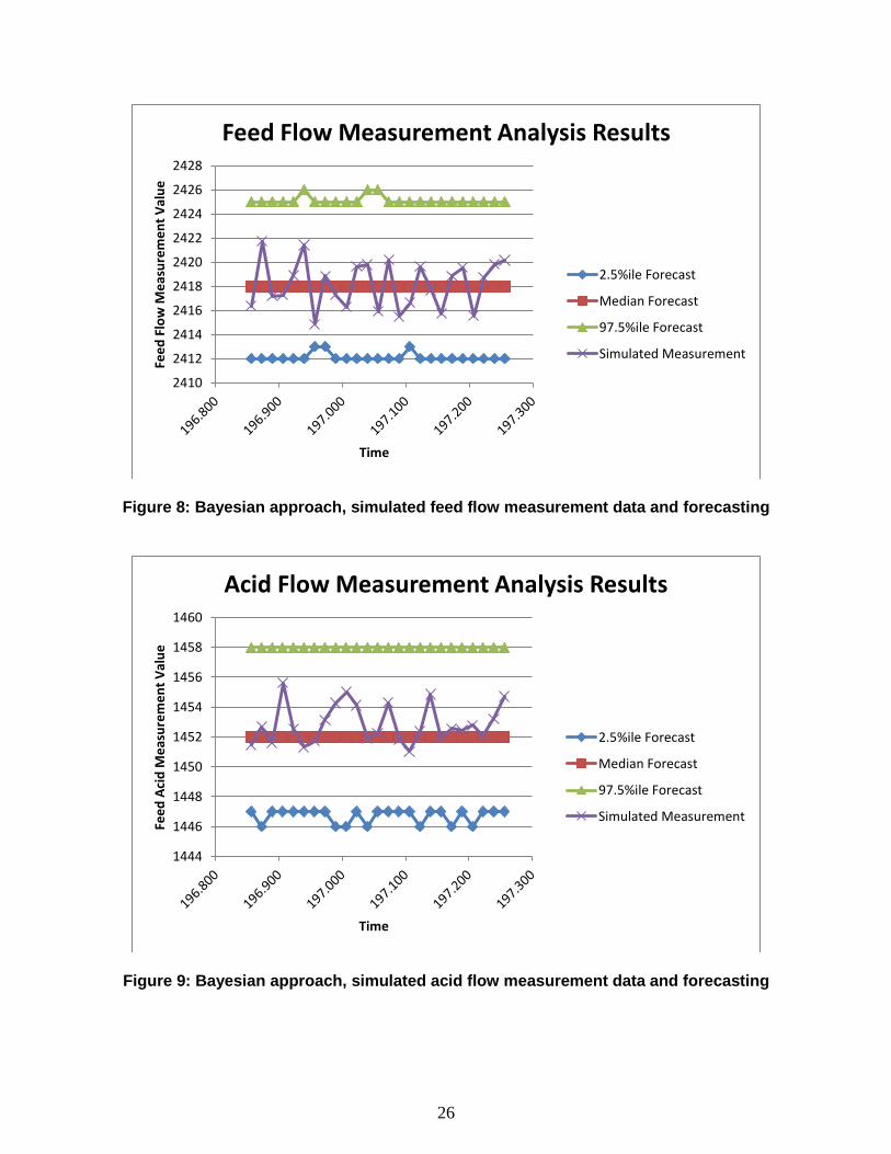
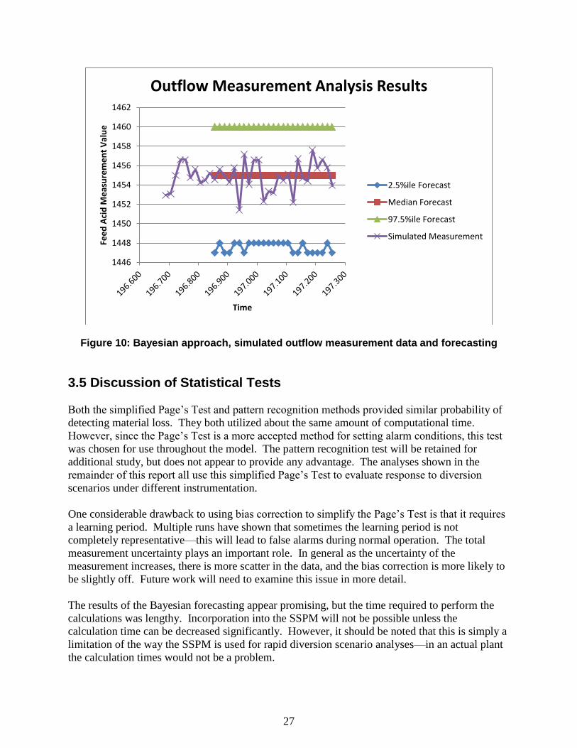
3.4.3 Bayesian Approach Results
The Bayesian approach examined the predictability of measurements in the UREX feed
adjustment tank during normal operation. Figures 7 through 10 present results for the
forecasting of measurements. The four figures show the forecast compared to the simulated
values for the inventory measurement, feed flow, acid flow, and outflow respectively. The
median predictions are all very close to the simulated data, and the 95% credibility intervals are
very tight. Since the true flow rate and inventory values can never be truly known, the best one
can hope for without experimental verification is the ability to predict the simulated
measurements that have been provided. This method can be extended to use the predicted values
to set alarm conditions for material loss. An actual plant can use past results or results from cold
startup for verification.
Figure 7: Bayesian approach, simulated inventory measurement data and forecasting
1880
2080
2280
2480
2680
2880
3080
3280
Fee
d F
low
Me
asu
rem
en
t V
alu
e
Time
Inventory Measurement Analysis Results
2.5%ile Forecast
Median Forecast
97.5%ile Forecast
Simulated Measurement
26
Figure 8: Bayesian approach, simulated feed flow measurement data and forecasting
Figure 9: Bayesian approach, simulated acid flow measurement data and forecasting
2410
2412
2414
2416
2418
2420
2422
2424
2426
2428Fe
ed
Flo
w M
eas
ure
me
nt
Val
ue
Time
Feed Flow Measurement Analysis Results
2.5%ile Forecast
Median Forecast
97.5%ile Forecast
Simulated Measurement
1444
1446
1448
1450
1452
1454
1456
1458
1460
Fee
d A
cid
Me
asu
rem
en
t V
alu
e
Time
Acid Flow Measurement Analysis Results
2.5%ile Forecast
Median Forecast
97.5%ile Forecast
Simulated Measurement
27
Figure 10: Bayesian approach, simulated outflow measurement data and forecasting
3.5 Discussion of Statistical Tests
Both the simplified Page‘s Test and pattern recognition methods provided similar probability of
detecting material loss. They both utilized about the same amount of computational time.
However, since the Page‘s Test is a more accepted method for setting alarm conditions, this test
was chosen for use throughout the model. The pattern recognition test will be retained for
additional study, but does not appear to provide any advantage. The analyses shown in the
remainder of this report all use this simplified Page‘s Test to evaluate response to diversion
scenarios under different instrumentation.
One considerable drawback to using bias correction to simplify the Page‘s Test is that it requires
a learning period. Multiple runs have shown that sometimes the learning period is not
completely representative—this will lead to false alarms during normal operation. The total
measurement uncertainty plays an important role. In general as the uncertainty of the
measurement increases, there is more scatter in the data, and the bias correction is more likely to
be slightly off. Future work will need to examine this issue in more detail.
The results of the Bayesian forecasting appear promising, but the time required to perform the
calculations was lengthy. Incorporation into the SSPM will not be possible unless the
calculation time can be decreased significantly. However, it should be noted that this is simply a
limitation of the way the SSPM is used for rapid diversion scenario analyses—in an actual plant
the calculation times would not be a problem.
1446
1448
1450
1452
1454
1456
1458
1460
1462Fe
ed
Aci
d M
eas
ure
me
nt
Val
ue
Time
Outflow Measurement Analysis Results
2.5%ile Forecast
Median Forecast
97.5%ile Forecast
Simulated Measurement

28
There are a few options for improving the calculation time of the Bayesian approach. The
current algorithm could be programmed directly in Simulink, or a compatible programming
language could be used. Also, the calculation should only focus on predicting the CuSum ID as
opposed to individual flow rate measurements. Future work should examine these methods of
optimization as well as how the Bayesian approach will respond in various diversion scenarios.

29
4.0 Analysis of New Measurement Technologies
As new measurement technologies are developed or as existing technologies improve, plant
monitoring may improve. Assessment of these technologies requires a systems study since a
large number of measurements typically come together to calculate an ID—an improvement in
one area may not necessarily improve the overall calculation if the weakest areas of the plant are
not addressed.
The SSPM was used to evaluate the impact that these new technologies can have on safeguards.
Part of the purpose of this analysis is to help guide the development of new technologies in the
Fuel Cycle Technologies program. The following sections describe the new technologies
currently being developed and show an analysis of their impact on plant monitoring. The
sections are broken down by type of measurement.
4.1 Used Nuclear Fuel Measurements
Past work [14,15] has consistently found that the absence of precision measurements of actinides
in used fuel is one of the current weaknesses of materials accountability. Precision
measurements cannot be taken until the fuel is dissolved and reaches the accountability tank. As
a result, an ID cannot be calculated with much precision on the front end of the plant. For this
reason operators rely on item accounting, containment, and surveillance of fuel at the front end.
Actinide measurements are particularly difficult on used fuel due to the high radiation
background and self-shielding of the material. Past and current work is examining a number of
non-destructive measurement techniques for potential use in improving the measurement of
actinides in used fuel [15]. Four such techniques are being supported by the MPACT working
group: Lead Slowing Down Spectroscopy (LSDS), Noble Gas Detectors, Fast Neutron
Multiplicity, and Compton Veto.
For this work, the individual technologies were not the focus, rather the modeling focused on
looking at the effects of improving the uncertainty of the measurement. This parametric study
shows the goals that the new technologies should attempt to meet. Experimental results of the
four technologies can be used to determine which have the best chance of reaching the goal.
A factor complicating this analysis is that an ID calculation requires the used fuel input
measurement, the accountability tank and other output measurements, and the inventory
measurements of all vessels in the front end. The inventory is not measured in existing plants, so
it would either need to be estimated or measured as well. Measurement of actinides while
undergoing dissolution would be extremely difficult due to the inability to sample and the
difficult geometry. Therefore, this inventory measurement can only feasibly be estimated from
the original used fuel measurement. Batch processing will be easier for accounting in this
manner than continuous dissolution, so a series of batch dissolver tanks were used in the model.
For this analysis, it was assumed that the inventory measurements could be estimated with the
same random and systematic error as the used fuel measurement.

30
A number of runs were completed with a diversion of material from the surge tank right before
the accountability tank in MBA1. The goal was to determine the detection limits for protracted
diversions. In all cases, a total of 8 kg of plutonium was removed. In parallel, the process
monitoring bulk material balances were used to determine how they may fill in gaps in anomaly
detection. Table 3 shows the result of the analysis for various measurement uncertainties.
Used Fuel
Measurement
Longest Protracted
Diversion Detected
r=10%, s=10% ~4 h
r=5%, s=5% ~8 h
r=1%, s=1% ~320 h
r=0.5%, s=0.5% ~640 h
Table 3: Used nuclear fuel measurement analysis
At the 10% and 5% error levels for the used fuel measurement, the uncertainty was so large that
only very abrupt diversions could be detected. At the 1% error level, a 320 hour diversion of 1
significant quantity (SQ) could be detected, and at the 0.5% error level, a 640 hour protracted
diversion of 1 SQ could be detected. The significant improvement for the bottom two (beyond
the ratio of the errors) is due to the fact that the measurement of Pu in used fuel storage is driving
the overall uncertainty. For large errors, the uncertainty of the Pu measurement in storage is
equal to or greater than the amount of Pu diverted. As the error comes down and the inventory
uncertainty is well below the amount of Pu diverted, detection sensitivity increases. This non-
linear relationship is part of the reason why systems studies like this are required.
Based on these results, a used fuel measurement must reach 1% in order to be able to provide
protection against protracted diversions, but even at these levels, longer protracted diversions
would not be detected. However, the results in Table 3 do not show the use of process
monitoring data. If mass or volume balances are taken using the bulk process monitoring data
with uncertainties near 0.1%, the longest diversion detected is near 4000 hours, which is equal to
about 8 months of plant operations (taking into account down time).
Bulk measurements do not provide complete protection since it is possible for material to be
diverted and replaced with surrogates. Process monitoring provides a significant advantage for
monitoring direct material loss only. If it is not possible to reduce the used fuel plutonium
measurement significantly, plants will likely need to continue to rely on containment and
surveillance to ensure the area has not been tampered with.
4.2 Precision NDA Measurements
Completing a plutonium mass balance requires knowledge of the inventory of material within an
MBA. For a more complex plant like UREX+ with multiple extraction steps, the internal plant
can contain many processing vessels. Sampling of every area is impractical, and it is very
difficult to get a representative sample is some locations. New non destructive analysis (NDA)

31
measurements that can estimate plutonium content without disturbing operations could be
valuable.
The MPACT campaign is investigating three new measurement technologies that may be useful
for this goal: microcalorimetry, Compton veto, and the multi-isotope process (MIP) monitor. In
addition, the Separations campaign is evaluating the UV-VIS technique for on-line process
monitoring. The following outlines the uncertainty goals for these technologies to provide a
benefit to the safeguards system.
For the front end of the plant (MBA1), the previous section already described the goals for
improvement. The assumption was made that the measurement uncertainty on the used fuel
would be equal to the uncertainty of the inventory of the dissolver tanks. Therefore,
measurement uncertainty of plutonium in the dissolver tanks should achieve 1% or better to
provide any value to the system. Because the amount of plutonium in the dissolver tanks is so
large, this measurement drives the overall mass balance just as much as the used fuel
measurement.
For MBA2, previous work determined that a number of locations process small or trace amounts
of plutonium [1], and these areas can have large measurement uncertainties without affecting the
overall measurement error. In order to test this more formally, the model was used to
parametrically change the measurement errors and look at the effect on the CuSum ID error bars.
To start, all of the tanks processing large amounts of plutonium were assumed to be sampled and
measured at low uncertainty (at 0.2% random and systematic error). The plutonium in all
remaining processing units, contactor banks, and tanks in MBA2 was assumed to be measured to
2%, 5%, 10%, and 20% over the same diversion scenario. Figure 11 shows the areas that were
varied in this study.

32
Figure 11: MBA2 with areas processing small (green) and large (yellow) quantities of plutonium
Figure 12 shows the CuSum ID plots from the analyses assuming the small inventory
measurements are at 2%, 5%, 10%, and 20%. The fact that the magnitude of the error bars does
not change show that increasing the measurement uncertainty has almost no effect on the overall
uncertainty. Also, the random scatter in the data does not increase visually. Therefore, these
locations in MBA2 only require a plutonium measurement at 20% or better in order to achieve
near real time accountability (NRTA). A number of simpler technologies can easily achieve this
level of uncertainty.

33
Figure 12: Parametric analysis results showing little difference in error bars as the uncertainty increases for areas processing small quantities of plutonium
4.3 Sampling Points
Traditional accounting from sampling at key tanks can be a lengthy process for a few reasons:
First, the tanks need to be mixed thoroughly to get representative samples. Second, the
measurement requires chemical separations first before running through a mass spectrometer.
Third, the use of mL-sized samples poses radiation hazards that may slow down the progress.
For all of these reasons, traditional sampling requires a lot of time for analytical staff.
Proposing more sampling points will require improvements in all three areas. Methods for
getting representative samples in shorter times or through well-designed pauses in operation will
be required. Measurement technologies that do not need to do chemical separations or
techniques for automating the separations will help to speed the processing time. Finally, the use
of mL sampling will help to reduce radiation hazards and reduce waste from the analytical lab.
These techniques are outside the scope of this report but are investigated in a parallel project
(reference 5) and in references 16 and 17. Such advanced sampling technologies will play an
important role in developing a near real time plant monitoring system.
2% Errors 5% Errors
10% Errors 20% Errors

34
4.4 Discussion
Any potential improvements to the front end of reprocessing depend on improving the used fuel
measurement. Bulk mass measurements are useful in the absence of a better used fuel
measurement, but they will still rely on containment and physical protection on the front end.
Optimization of MBA2 can allow for a near real time system without requiring expensive
equipment throughout the plant. A majority of the areas in MBA2 require a plutonium
measurement with uncertainty of 20%, and many simple technologies can be used. In many
cases, process monitoring measurements coupled with a simple spectroscopic technique will be
adequate. A relatively small number of additional tanks will need to be sampled, but current
work should allow for additional sampling without increased cost.

35
5.0 Safeguards and Security Integration
The previous sections describe materials accountancy, but material measurements are only one
part of a plant‘s defense against material loss. Reprocessing plants also contain extensive
physical protection barriers and administrative procedures to protect against loss. True diversion
scenario analyses must look at how the material, once removed, will make it off-site. Existing
plants do not integrate these various systems extensively.
The SSPM has been used to setup a physical protection system (PPS) to examine how material
balances and administrative procedures can be better integrated into the overall plant monitoring
system. The following sections describe the setup for the PPS, administrative procedures, the
model setup in the SSPM, and results under various diversion scenarios. ATLAS [18]
(Adversary Time-Line Analysis System) was used to design a hypothetical PPS for both MBAs
in the SSPM.
The modeling for this work focused on theft or diversion of material by an insider adversary
during normal facility operations. The insider adversary has access to and knowledge of the
plant’s operations and is assumed to be a passive, non-violent insider who will undertake
diversion activities without the use of any tools. For each security layer, descriptions of the
protection elements and associated hypothetical performance values for delay times and
detection probabilities were developed for the ATLAS model. Delay times and detection
probabilities were tailored specifically for the insider, leading to two key assumptions: (1) the
delay times are analogous to adversary task times for an insider; and (2) traditional detection
methods would not be effective against a knowledgeable insider, so detection is based primarily
on observations of unauthorized activities and attempts at unauthorized access. Performance
values for the model are given in a limited release appendix.
5.1 MBA1 ATLAS Model
The front end includes fuel receipt through the accountability tank, and is contained entirely in
the fuel building. Fuel is received and stored on-site in the fuel building to maintain continuous
operation. Fuel chopping, dissolution, and accountability would occur in a hot cell or canyon.
A surge tank regulates batch flow into the accountability tank where samples can be taken for
precise analytical measurements. The feed out of the accountability tank leaves the fuel building
to go to a different building where separation occurs.
Figure 13 is the adversary sequence diagram (ASD) for the front end of the facility. An ASD is a
two-dimensional graphical representation of all PPS layers and protection elements defined for a
facility, as well as all possible adversary paths through the facility. The target material is
chopped, used fuel pieces containing uranium and plutonium oxide. This target is indicated at
the bottom of the ASD in Figure 13. The type of target is an item process line (IPL) and the
primary safeguard for detection is input verification of the target material (by bulk mass
balance).

36
Figure 13: Adversary sequence diagram for the front end
Security Layers and Physical Protection System Elements- MBA1
The protection elements between the target area and the fuel building work area include the
following:
Surface (SUR)- Hot cell wall
The insider adversary cannot penetrate this barrier because he has no tools.
Door (DOR)- Hot cell door:
The adversary has authorized access and can open an electronically coded lock on the
vault-type door. The door position monitor may alarm or may be disabled, but
assessment of unauthorized activity is needed. General observation and a portal SNM
monitor on exit may provide detection of unauthorized activity.
Door (DOR)- Canyon ceiling access:
The adversary may have authorized access and can attempt to obtain the padlock key for
the ceiling access. The door position monitor may alarm or may be disabled, but the
assessment of unauthorized activity is needed. No general observation is available to
provide detection of unauthorized activity.
The protection elements between the fuel building work area and the protected area (PA) include
the following:
37
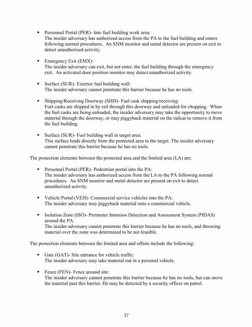
Personnel Portal (PER)- Into fuel building work area:
The insider adversary has authorized access from the PA to the fuel building and enters
following normal procedures. An SNM monitor and metal detector are present on exit to
detect unauthorized activity.
Emergency Exit (EMX):
The insider adversary can exit, but not enter, the fuel building through the emergency
exit. An activated door position monitor may detect unauthorized activity.
Surface (SUR)- Exterior fuel building wall:
The insider adversary cannot penetrate this barrier because he has no tools.
Shipping/Receiving Doorway (SHD)- Fuel cask shipping/receiving:
Fuel casks are shipped in by rail through this doorway and unloaded for chopping. When
the fuel casks are being unloaded, the insider adversary may take the opportunity to move
material through the doorway, or may piggyback material on the railcar to remove it from
the fuel building.
Surface (SUR)- Fuel building wall in target area:
This surface leads directly from the protected area to the target. The insider adversary
cannot penetrate this barrier because he has no tools.
The protection elements between the protected area and the limited area (LA) are:
Personnel Portal (PER)- Pedestrian portal into the PA:
The insider adversary has authorized access from the LA to the PA following normal
procedures. An SNM monitor and metal detector are present on exit to detect
unauthorized activity.
Vehicle Portal (VEH)- Commercial service vehicles into the PA:
The insider adversary may piggyback material onto a commercial vehicle.
Isolation Zone (ISO)- Perimeter Intrusion Detection and Assessment System (PIDAS)
around the PA:
The insider adversary cannot penetrate this barrier because he has no tools, and throwing
material over the zone was determined to be not feasible.
The protection elements between the limited area and offsite include the following:
Gate (GAT)- Site entrance for vehicle traffic:
The insider adversary may take material out in a personal vehicle.
Fence (FEN)- Fence around site:
The insider adversary cannot penetrate this barrier because he has no tools, but can move
the material past this barrier. He may be detected by a security officer on patrol.

38
Gate (GAT)- Rail gate for shipping casks:
Fuel casks are shipped in and out through this gate. The insider adversary may take the
opportunity to move material through the doorway or piggyback material on a railcar.
5.2 MBA2 ATLAS Model
The separations portion of the plant includes all of the chemical processes to separate out the
uranium and transuranics (TRU). The separations are undertaken in the extraction building, with
product and waste streams sent via tunnel to other buildings for additional processing. UREX
feed enters the separations building through a tunnel from the fuel building. After entering the
separation building, it is passed through a series of contactors and strippers to successively
separate out different species. The first separation step co-extracts U and Tc, which are then sent
to waste processing. The raffinate is then sent through a TRUEX extraction process, which co-
extracts the TRU and lanthanides. The final separation step is a TALSPEAK process, where the
lanthanides are separated out, leaving a TRU product. The TRU product tank is contained within
a hot cell or canyon. Figure 14 is the ASD for the separations portion of the facility. The target
material is TRU solution in a product tank, as shown at the bottom of the figure. The type of
target is a bulk process line (BPL).
Figure 14: Adversary sequence diagram for separations

39
Security Layers and Physical Protection System Elements- MBA2
The protection elements between the target area and the extraction building include the
following:
Surface (SUR)- Hot cell wall
The insider adversary cannot penetrate this barrier because he has no tools.
Door (DOR)- Hot cell door:
The adversary has authorized access and can open an electronically coded lock on the
vault-type door. The door position monitor may alarm or may be disabled, but
assessment of unauthorized activity is needed. General observation and a portal SNM
monitor on exit may provide detection of unauthorized activity.
Door (DOR)- Canyon ceiling access:
The adversary may have authorized access and can attempt to obtain the padlock key for
the vault-type door. The door position monitor may alarm or may be disabled, but the
assessment of unauthorized activity is needed. No general observation is available to
provide detection of unauthorized activity.
The protection elements between the extraction building and the protected area include the
following:
Personnel Portal (PER)- Into extraction building:
The insider adversary has authorized access from the PA into the extraction building and
enters following normal procedures. An SNM monitor and metal detector are present on
exit to detect unauthorized activity.
Emergency Exit (EMX):
The insider adversary can exit, but not enter, the extraction building through the
emergency exit. An activated door position monitor may detect unauthorized activity.
Surface (SUR)- Exterior fuel building wall:
The insider adversary cannot penetrate this barrier because he has no tools.
Tunnel (TUN)- Tunnel to U/TRU solidification and repackaging:
The insider adversary could send material through a tunnel from the extraction building
to another building in the protected area. This tunnel leads directly from the target area
into the protected area. It is not man-passable. No detection systems exist in the tunnel.
Surface (SUR)- Extraction building wall in target area:
This surface leads directly from the protected area to the target. The insider adversary
cannot penetrate this barrier because he has no tools.
The protection elements between the protected area and the limited area are:

40
Personnel Portal (PER)- Pedestrian portal into the PA:
The insider adversary has authorized access into the PA following normal procedures.
An SNM monitor and metal detector are present on exit to detect unauthorized activity.
Vehicle Portal (VEH)- Commercial service vehicles into the PA:
The insider adversary may piggyback material onto a commercial vehicle.
Isolation Zone (ISO)- Perimeter Intrusion Detection and Assessment System (PIDAS)
around the PA:
The insider adversary cannot penetrate this barrier because he has no tools.
Tunnel (TUN)- Liquid waste and U/Tc tunnels
The insider adversary could send material through either of the two tunnels from the
extraction building to a building in the limited area. These tunnels lead directly from the
target area into the limited area. They are not man-passable. No detection systems exist
in these tunnels.
The protection elements between the limited area and offsite include the following:
Gate (GAT)- Site entrance for vehicle traffic
The insider adversary may take material out in a personal vehicle.
Fence (FEN)- Fence around site
The insider adversary cannot penetrate this barrier because he has no tools, but can move
the material past this barrier. He may be detected by a security officer on patrol.
Gate (GAT)- Rail gate for shipping casks
Fuel casks are shipped in and out through this gate. The insider adversary may take the
opportunity to move material through the doorway or piggyback material on a railcar.
5.3 MC&A Procedures & Human Reliability
Traditional physical security measures are largely ineffective against an insider adversary;
however, MC&A procedures can serve as a type of sensor to bolster both delay and detection
against the insider threat. To assess the added value of MC&A procedures for material
protection, these procedures were integrated into the SSPM. A human reliability analysis (HRA)
model was used for this integration. HRA has been used to characterize procedures at nuclear
power plants [19], and recent work has extended this method to MC&A procedures at nuclear
facilities [20]. This method is useful for procedures that require a person to check the status of a
critical asset. For nuclear power plant procedures, baseline human error probabilities (BHEP)
have been established for several different checking procedures. Many of these activities are
analogous to MC&A activities, and as such, BHEPs have been assigned to a variety of
administrative MC&A activities that may occur at nuclear facilities. A daily administrative
check (DAC) with a BHEP of 0.10 was integrated into the SSPM. This means that the baseline

41
probability of detecting an anomaly with a DAC is 0.90, assuming there is enough data present to
show the anomaly.
HRA prescribes a positive dependence relationship between checking activities, meaning the
success of one activity depends on the success of the activity immediately preceding it. In the
context of a DAC, the failure to detect an anomaly one day increases the probability that the
anomaly will not be detected the next day. The strength of this dependence relationship is
described by the dependency factor. Equation 10 has been adapted from the general failure
equation and gives the mathematical formulation for this positive dependence relationship. It
describes the probability that an anomaly will not be detected on day n, given that the anomaly
was not detected the previous day.
( | )
(Eq. 10)
where a is the dependency factor, with values of 19, 6, and 1, corresponding to low, moderate
and high dependency, respectively. This equation was used to calculate daily probabilities of
MC&A detection for the duration of the simulation in the SSPM.
The complication is that the calculation for HRA cannot be applied until there is enough data
present to detect the anomaly. In the case of a protracted diversion, many inventory balances
may be required until there is enough confidence that the diversion should be detected. In order
to model this, an additional factor must be used that represents the detection probability as a
function of time, based on the diversion fraction.
While the probability of detection decreases for each MC&A instance according to the positive
dependence relationship given in Equation 10, the cumulative detection probability increases
according to Equation 11,
n
icumulativeD PP NDi
1,
1 (Eq. 11)
where PNDi
is the probability of non-detection for each MC&A event, or the complement of
the detection probability. Thus as the length of the scenario timeline increases, the cumulative
probability of detecting the theft also increases, despite the drop in detection probability for each
MC&A event, because the adversary is subjected to additional MC&A checks.
5.4 Integration in the SSPM
The primary goal of the integration is to determine how additional plant data can improve the
overall plant monitoring system. This was accomplished by creating PPS subsystems whose
state would change if an alarm occurred in any material balance calculation or in the
administrative procedures. The following two sections describe how these subsystems were
setup in the model.

42
5.4.1 MC&A Administrative Procedures & Human Reliability
Only one example of an administrative procedure at a reprocessing plant was modeled in the
SSPM, the daily administrative check (DAC). This check was assumed to occur once every 24
hours. The assumption is that a plant administrator is reviewing the plant data once daily, and
this data comes from a variety of sources. The administrator may directly monitor the CuSum
ID of various areas in the plant, shipper-receiver data, material movements, cold chemical
supply, etc. This administrator is likely to have intimate knowledge of the plant which may
allow him to identify an anomaly before the material balance system can automatically produce
an alarm.
The DAC subsystem is shown in Figure 15. This calculation only starts when an actual
diversion begins in the model. The probability of detection is 0.9 multiplied by a value that
depends on the diversion fraction and the amount of time that has passed. Examination of
numerous diversion scenarios has shown that the diversion fraction, multiplied by 10, multiplied
by the time since the diversion started (in hours) is an appropriate multiplier (but it must saturate
out at 1.0). The goal is to simulate how additional mass balance periods during a diversion make
it increasingly likely to visually detect the event. The HRA calculations are used in the triggered
subsystems to calculate a detection probability once every 24 hours. The dependency is
currently set up as a constant, but could be changed for each procedure. If an alarm occurs, the
output signal changes from zero to one.
Figure 15: Daily administrative check subsystem
When the alarm condition signal changes, the model is programmed to generate a popup window
that tells what the alarm is (Daily Administrative Check) and when it occurred. The alarm
condition is one of the input feeds into the PPS system that can change the state of the system.
Although this is just one example, this template can be copied and modified for other types of
administrative procedures that may occur at different time intervals. The alarm conditions from
each can be used to influence the PPS system state.

43
5.4.2 PPS System
The SSPM includes a number of locations from which material can be diverted. The diversion
scenario is defined by the user at the start of a run. Depending on where the diverted material is
coming from, the architecture for the PPS subsystems routes the diverted material through the
appropriate PPS system elements.
Figure 16 shows the PPS system subsystems for MBA1 and MBA2. The inputs into each
subsystem are the diverted material and three potential alarm signals: MBA alarm (plutonium
balance), process monitoring alarm (bulk balance), and the MC&A administrative procedures
alarm. These three alarms can all change the state of the PPS system. The window shown on the
right in figure 16 allows the user to define the particular diversion path through the PPS
elements. This window shows the options for MBA1. In addition to defining the path, the user
can also define if the material is held up in any one barrier to find a more optimal time to divert.
Figure 16: PPS subsystem inputs
The actual PPS for MBA1 and MBA2 (one level down in the model) are shown in Figures 17
and 18. These figures show the multiple pathways through which material can travel to get off-
site, all based on the ATLAS models described previously. The particular target is chopped fuel
in the process cell (hot cell) for MBA1 and the TRU product solution for MBA2.
Each particular barrier has a number of possible paths to get material out—based on the user
inputs, diverted material will only travel through one pathway. In some cases, the pathways can
go through multiple barriers. A delay block was used to represent the combination of penetration

44
time and delay time for that pathway. The delay times as shown later in the example diversion
scenarios are all hypothetical, but performance data from ATLAS is included in the limited
release appendix. In this manner the diverted material is routed through the diversion path
chosen by the user.
Each pathway has an alarm probability associated with it, although in some cases the probability
may be 0%. An embedded Matlab code (labeled ‗MBA PPS Alarm Messages‘ in the upper right
hand corner of the figures) contains all of the alarm probabilities for each pathway. If material is
traveling through that path, there is a finite chance of the alarm going off (as long as the
probability is greater than 0%). A random number generator is used to determine if an alarm is
indicated based on the associated alarm probability. An alarm is indicated with a message popup
window that gives the PPS element location and the alarm time. The embedded Matlab code is
shown in the limited release appendix.
The goal of this work is to examine how the integration of material balance data and
administrative procedures may improve the PPS by increasing the probability of timely detection
through tighter integration. Any potential alarms in the plutonium balance, the process
monitoring balance, or the administrative procedures subsystems will place the PPS system into
an alert state. Under an alert state, the detection probabilities of the PPS elements may increase
significantly. For example, the area of the plant may undergo scrutiny, guard rounds may
increase, or door combination codes may rotate. The alert state makes it more likely to detect the
particular diversion pathway so that the event can be stopped. This improvement extends
beyond security. If a vessel leak causes an alarm to go off, more intense scrutiny of the area will
show the problem and allow the operator to fix the vessel as soon as possible.
While the diversion pathways and detection probabilities for a particular adversary were modeled
in the SSPM, it is not currently setup to run an automated path analysis. The user defines the
path, but the current work has not attempted any down-select to determine credible diversion
scenarios. Future work can examine the path analysis to determine groups of diversion scenarios
that are of concern.

45
Figure 17: PPS for MBA1

46
Figure 18: PPS for MBA2

47
5.5 Diversion Scenarios
A number of diversion scenarios were run to test the concept of the integrated systems. These
runs included the culmination of all work previously described in the report, so the Page‘s Test
was used for the plutonium balance and bulk material balance alarms. A future plant design with
NRTA was also assumed. The diversion scenarios described looked at the effects of the alarms
on the PPS system.
5.5.1 Effect of Plutonium and Bulk Material Balance Alarms
Initially, only the process monitoring and plutonium balance system alarms were integrated into
the PPS. An abrupt diversion was set up for the MBA1 assuming that chopped fuel pieces were
removed from the hot cell. This diversion occurred over 24 hours (starting at hour 300) for a
total of 8 kg of plutonium. The material was assumed to be removed through the hot cell door,
then smuggled out on a rail car through shipping/receiving, and then out the rail gate. The
detection probabilities were arbitrarily assumed to be 25% for the hot cell door, 10% at
shipping/receiving, and 10% at the rail gate. Also it was assumed that two trips would be
required to get all the material out, so the probabilities were calculated every 10 hours.
Figure 19 shows the baseline results without integration of the material balance data. The left
graph shows the bulk CuSum ID for the Chopper location, and the right graph shows the
plutonium balance CuSum ID across MBA1. In this scenario, none of the PPS system elements
alarmed. The lower probabilities coupled with only two detection opportunities limited their
response.
Figure 19: Abrupt diversion from MBA1 without integrated systems—no PPS alarm blocks were indicated during the diversion
The same diversion scenario was run but with the integrated system that allowed for a alert state
to be reached. If an alarm signaled an alert state, the three PPS elements‘ detection probabilities
increase to 50%. Figure 20 shows these results. In this case, the process monitoring alarm
triggered an alert state 4 hours after the diversion started, and the plutonium balance was able to
signal an alarm after 24 hours. The increased detection probabilities led to 2 PPS alarms.
Shipping and receiving was able to detect the material diversion after 30 hours, and the site rail
gate detected the material transfer after 50 hours. Note that a lag time was programmed into the
model to simulate a delay time before a rail car would leave the facility.

48
Figure 20: Abrupt diversion from MBA1 with integrated systems—the process monitoring alarm triggers an alert state causing two PPS alarms
A protracted diversion scenario was examined to look at response times when material is
removed little by little over long periods of time. Due to the large volumes of liquid that must be
removed for one significant quantity of plutonium, it is very possible that many trips would be
needed for an adversary to remove the material. In this diversion scenario, 0.1% of the flow into
the stripper tank was diverted over 1600 hours (starting at hour 300). The material was assumed
to be removed from the process cell by the canyon ceiling access, then removed through the
emergency exit, and then smuggled onto a rail car to leave the facility. The detection
probabilities were arbitrarily assumed to be 5% for the ceiling access, 10% for the emergency
exit, and 5% for the rail car exit. The alert state was designed to increase these probabilities to
50% for all three. It was assumed that there would only be one chance per day to remove
material in this manner, so the detection probabilities were only calculated once every 24 hours.
Figure 21 shows the monitoring screen assuming that the materials accountancy and process
monitoring data is not linked to the PPS system. The detection probabilities for a knowledgeable
insider are low and remain low throughout the diversion. In fact, existing reprocessing plants
that cannot achieve low uncertainty for NRTA would probably not detect this material loss until
many months later at a plant flushout. Therefore, this could be representative of an existing
plant. However, due to the increased number of opportunities, all three PPS elements were able
to alarm. The ceiling access alarm was seen 180 hours after the start of the diversion, followed
by the rail gate alarm after 276 hours, and lastly the building emergency exit after 324 hours.
The PPS system was able to respond to this material diversion before half of a significant
quantity was removed.

49
Figure 21: Protracted diversion from MBA2 without integrated systems— PPS alarm blocks were indicated due to multiple detection opportunities
In comparison to the above results, the same diversion scenario was run assuming the integrated
system. Figure 22 shows the result. The process monitoring system alarmed 108 hours after the
diversion started, and the plutonium balance alarmed after 124 hours. The increased detection
probabilities (due to the alert state) led to an alarm at the Extraction Building emergency exit
immediately, and alarms at the canyon ceiling access and rail gate shortly thereafter. Note that
the diversion started at hour 300, but the PPS elements did not alarm until the alert state was
achieved.
The protracted diversion scenarios show that the integration of the materials accountancy alarms
can significantly speed up detection time in the PPS system elements. This example simply
highlights the idea, but actual results will be highly dependent on the facility design and actual
detection probabilities. These results also point out why an adversary would want to remove
material all at once as opposed to over multiple days. Although the probability of detecting
removal of a small quantity might be lower, repeatedly removing small amounts of material over
time eventually raises the cumulative probability of detection above the probability of detecting
an abrupt removal of a single larger quantity.

50
Figure 22: Protracted diversion from MBA2 with integrated systems— PPS alarm blocks were indicated earlier sue to the alert state
5.5.2 Effect of MC&A Administrative Procedures Alarms
The previous diversion scenarios did not take into account administrative procedures that may
indicate process discrepancies. The administrative procedures example that was put into the
model was a daily administrative check, so it will only occur once every 24 hours. Two
diversion scenarios were examined to determine if an administrative procedures alarm will
trigger an alert state. In both cases, the material balance alarms were disabled in the model.
The first scenario was an abrupt diversion of fuel pieces from MBA1 over 24 hours, for a total
diversion of 8 kg of plutonium (the same abrupt diversion as shown earlier). It was assumed that
material was removed twice during this diversion. Figure 23 shows the result from the run.
During this run, the daily administrative check signaled an alarm in the middle of the diversion.
This in turn triggered an alert state that indicated alarms in two of the PPS elements. A 24 hour
delay time was built into this run, which is why the PPS system elements alarmed after the
material was initially diverted. This result shows that the administrative procedures can enhance
the plant monitoring system by improving the detection timeliness.

51
Figure 23: Abrupt diversion from MBA1 with integrated systems—the administrative procedures alarm triggers an alert state causing two PPS alarms
The second scenario was a protracted diversion of the TRU surge tank solution over 1900 hours,
for a total of 8 kg of plutonium. Figure 24 shows the results from this run for the first 1000
hours. The administrative procedures signaled an alarm after 128 hours, but interestingly, one of
the PPS elements alarmed before that. The two other PPS elements appear to have been helped
by the alert state. Because of the large number of detection opportunities with this diversion
scenario, it is unclear how much the administrative procedures helped. However, there may be
examples of protracted material loss with abrupt removal from the facility that might benefit
more from the administrative procedures.
Figure 24: Protracted diversion from MBA2 with integrated systems—the administrative
procedures alarm triggers an alert state causing three PPS alarms
Both of the administrative procedures scenarios examined were the same scenarios as those
examined using the material balance alarms. In both cases, the process monitoring system was
able to signal an alarm first, but the administrative procedures were typically able to detect an
alarm before the plutonium balance. The case of a substitution diversion could be hidden from
the process monitoring system, so reliance on administrative procedures and plutonium balances
will still be required.
For the administrative procedures, the results are completely dependent on the detection
probabilities. As described earlier, these probabilities were linked to the fraction of material
diverted and based on an assumption that the probabilities grow with time as the diversion
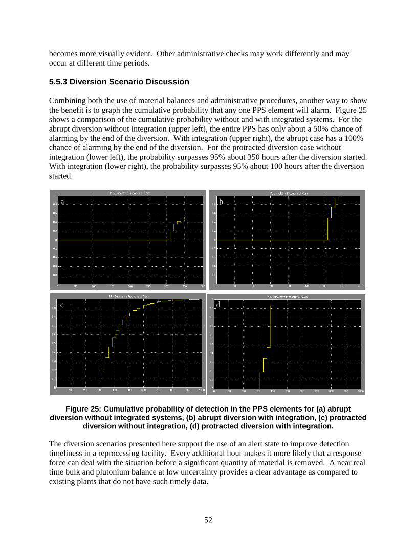
52
becomes more visually evident. Other administrative checks may work differently and may
occur at different time periods.
5.5.3 Diversion Scenario Discussion
Combining both the use of material balances and administrative procedures, another way to show
the benefit is to graph the cumulative probability that any one PPS element will alarm. Figure 25
shows a comparison of the cumulative probability without and with integrated systems. For the
abrupt diversion without integration (upper left), the entire PPS has only about a 50% chance of
alarming by the end of the diversion. With integration (upper right), the abrupt case has a 100%
chance of alarming by the end of the diversion. For the protracted diversion case without
integration (lower left), the probability surpasses 95% about 350 hours after the diversion started.
With integration (lower right), the probability surpasses 95% about 100 hours after the diversion
started.
Figure 25: Cumulative probability of detection in the PPS elements for (a) abrupt diversion without integrated systems, (b) abrupt diversion with integration, (c) protracted
diversion without integration, (d) protracted diversion with integration.
The diversion scenarios presented here support the use of an alert state to improve detection
timeliness in a reprocessing facility. Every additional hour makes it more likely that a response
force can deal with the situation before a significant quantity of material is removed. A near real
time bulk and plutonium balance at low uncertainty provides a clear advantage as compared to
existing plants that do not have such timely data.
a b
c d

53
The administrative procedures provide a timeliness advantage in the absence of near real time
material balances. The process monitoring system appears to provide the most timely
information and alarms. However, bulk material balances cannot detect a substitution diversion.
For that case, the administrative procedures may be the first to alarm.

54
6.0 Conclusions A number of modifications to the SSPM were made in order to provide the analyses shown here.
Three statistical techniques were evaluated for setting alarm conditions for material loss. The
pattern recognition and Bayesian approaches show promise, but both will require more testing
under diversion scenarios. It is unclear if both approaches will hold up under the diverse
conditions in a reprocessing plant. The Bayesian approach suffered from a longer computational
time that can be addressed. Since there is much more rigor behind the Page‘s Test, this test was
used throughout the model for setting alarm conditions. The simplified version of Page‘s Test
does lead to some limitations in the model, but it has been useful for diversion scenarios
analyses.
The SSPM was used to determine the design requirements for achieving NRTA in reprocessing
to low uncertainty. A used fuel measurement will be required to allow NRTA on the front end,
but the measurement uncertainty for plutonium must be at or below 1% in order to provide
protection against protracted diversions. If this goal cannot be achieved, it will be better to rely
only on process monitoring balances, containment, and surveillance of the front end.
For the rest of the separations portion of a plant, achieving NRTA requires inventory
measurements throughout. Fortunately, a vast majority of the processing units (including all
contactors, non-plutonium bearing product and waste tanks, and recycle tanks) only require a
plutonium measurement with uncertainty near 20%. These areas are less statistically significant
since they process only small quantities of plutonium. The coupling of process monitoring
measurement along with a simple and inexpensive NDA technique can work in these locations.
Techniques like gamma spectroscopy or UV-Vis-NIR spectroscopy may be useful here. Only a
relatively small number of tanks are processing large enough quantities of plutonium to need
sampling and precision analytical measurements.
The SSPM was also modified to model PPS and administrative procedures that are also used to
protect reprocessing plants from material loss. A PPS system is now included that shows
pathways through which material may follow to exit both MBAs. An example administrative
procedure was modeled to demonstrate the additional safeguard that is provided in plants. The
material balances from the process monitoring system and plutonium accountability system were
used with the administrative procedures to improve the overall PPS. Material balance or
administrative procedure alarms trigger an alert state in the plant which increases the probability
of the detection of material loss through the various PPS elements.
Diversion scenario testing showed that without the integration of the material balance and
administrative procedures, the PPS elements were much less likely to alarm. Abrupt diversions
in particular could occur without detection, but protracted diversions were usually detected due
to multiple detection opportunities. With integrated systems, the PPS elements in all scenarios
alarmed earlier. It should be noted that the process monitoring system was the most timely for
generating alarms, but in cases of substitution diversions, the plutonium balance or
administrative procedures would be required to trigger an alert state.

55
7.0 References
1. B.B. Cipiti, ―Separations and Safeguards Performance Modeling for Advanced
Reprocessing Facility Design,‖ Journal of Nuclear Materials Management, 39/2 pp. 4-14,
March 2011.
2. B.B. Cipiti and F.A. Duran, ―Integrated Safeguards and Security for Improved Plant
Monitoring at a Fuel Recycling Facility,‖ SAND2010-7681 (October 2010).
3. B.B. Cipiti, ―Separations and Safeguards Performance Model,‖ SAND2009-4896 (August
2009).
4. B.B. Cipiti and O.R. Zinaman, ―Separations and Safeguards Model Integration,‖
SAND2010-5962 (September 2010).
5. B.B. Cipiti, ―Transformative Monitoring Approaches for Reprocessing,‖ SAND2011-6578
(September 2011).
6. R.H. Rainey and S.B. Watson, ―Modification of the SEPHIS Computer Code for
Calculating the PUREX Solvent Extraction System,‖ ORNL-TM-5123, Oak Ridge
National Laboratory (1975).
7. M.C. Regalbuto et al., "Solvent Extraction Process Development for Partitioning and
Transmutation of Spent Fuel," Actinide and Fission Product Partitioning and
Transmutation, Eighth Information Exchange Meeting, Nuclear Energy Agency
Organization for Economic Co-operation and Development, Las Vegas, Nevada (2004).
8. T.P. Speed and D. Culpin, ―The Role of Statistics in Nuclear Materials Accounting: Issues
and Problems,‖ Journal of the Royal Statistical Society A, 149/4 pp. 281-313 (1986).
9. B.J. Jones, ―Near Real Time Materials Accountancy using SITMUF and a Joint Page‘s
Test: Comparison with MUF and CUMUF Tests,‖ ESARDA Bulletin, 15 (1988).
10. N.L. Ricker, ―Dynamic Model of the UREX+ Process,‖ unpublished (2006).
11. T. Burr & M.S. Hamada, ―Development of Pattern Recognition for Combining Multiple
Safeguards Subsystems,‖ Los Alamos National Laboratory, LAUR-11-03925 (2011).
12. D.J. Lunn, A. Thomas, N. Best, and D. Spiegalhalter, ―WinBUGS -- a Bayesian Modeling
Framework: Concepts, Structure, and Extensibility,‖ Statistics and Computing, 10, 325-337
(2000).
13. A. Gelman, J.B. Carlin, H.S. Stern, and D.B. Rubin, Bayesian Data Analysis, Second
Edition (2003).
14. L.E. Smith et al., ―AFCI Safeguards Enhancement Study: Technology Development
Roadmap,‖ PNNL-18099, Pacific Northwest National Laboratories, Richland WA
(December 2008).
15. M.E. Abhold et al., ―Survey of Seven Measurement Techniques for Quantifying the Fissile
Content of Spent Fuel,‖ LA-UR-07-3336, Los Alamos National Laboratory, Los Alamos
NM (2007).
16. D. Bowers et al., ―Enhanced AFCI Sampling, Analysis, and Safeguards Technology
Review,‖ INL/EXT-09-16997 (September 2009).
17. D. Meikrantz and J. Svoboda, ―Enhanced Sampling and Analysis, Selection of Technology
for Testing,‖ INL/EXT-10-17919 (February 2010).
18. ATLAS (Adversary Time-Line Analysis System) software, Version 4.4, Sandia National
Laboratories, Copyright 2003-2009.

56
19. A.D. Swain III and H.E. Guttman, “Handbook of Human Reliability Analysis with
Emphasis on Nuclear Power Plants,” SAND90-0200 (1983).
20. F.A. Durán, Probabalistic Basis and Assessment Methodology for Effectiveness of
Protecting Nuclear Materials, PhD Dissertation, The University of Texas at Austin (2010).

57
Distribution
1 Mark Mullen
Los Alamos National Laboratory
P.O. Box 1663
Los Alamos, NM 87545
1 Daniel Vega
U.S. Department of Energy
1000 Independence Ave. SW
Washington, DC 20585
1 Tom Burr
Los Alamos National Laboratory
P.O. Box 1663
Los Alamos, NM 87545
1 Trond Bjornard
Idaho National Laboratory
2525 Fremont Ave.
Idaho Falls, ID 83415
1 Brad Key
QinetiQ
100 Sun Ave. NE, Suite 500
Albuquerque, NM 87109-4670
1 MS 0747 Ben Cipiti, 6223
1 MS 0747 Ken Sorenson, 6223
1 MS 0757 Felicia Duran, 6612
1 MS 0757 Rebecca Ward, 6612
1 MS 0757 Carla Ulibarri, 6612
1 MS 0757 Sabina Jordan, 6612
1 MS 0757 Greg Wyss, 6612
1 MS 1136 Bobby Middleton, 6221
1 MS 0899 Technical Library, 9536 (electronic copy)