1

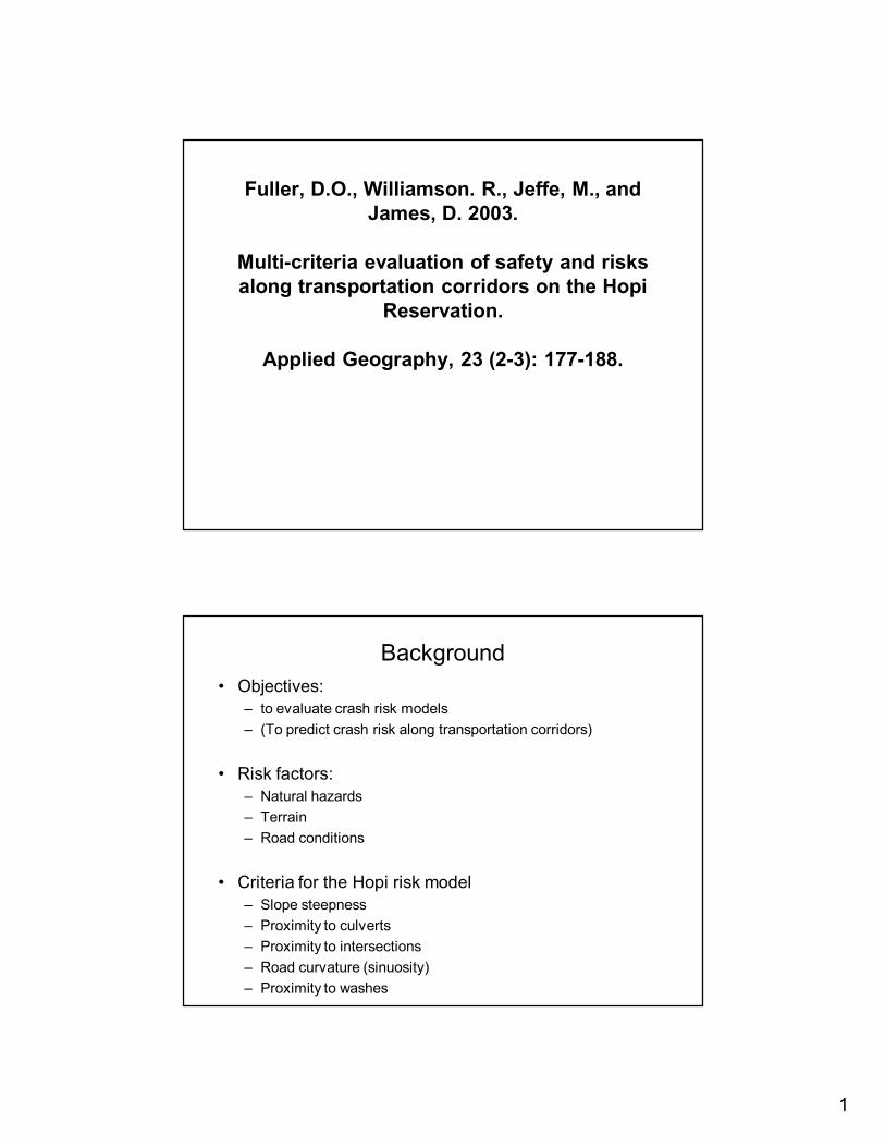
Fuller, D.O., Williamson. R., Jeffe, M., and James, D. 2003.

Multi­criteria evaluation of safety and risks along transportation corridors on the Hopi

Reservation.

Applied Geography, 23 (2­3): 177­188.

Background • Objectives:

– to evaluate crash risk models – (To predict crash risk along transportation corridors)

• Risk factors: – Natural hazards – Terrain – Road conditions

• Criteria for the Hopi risk model – Slope steepness – Proximity to culverts – Proximity to intersections – Road curvature (sinuosity) – Proximity to washes

2

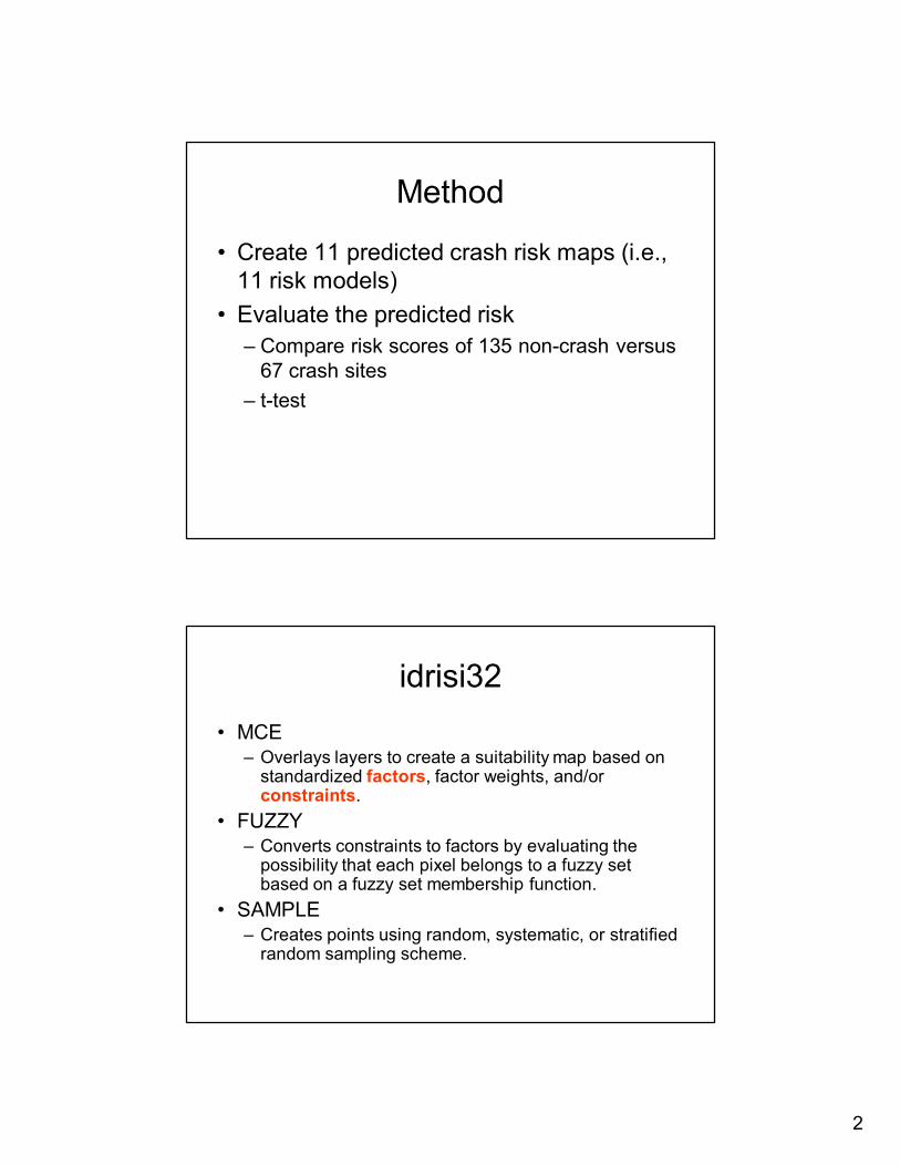
Method

• Create 11 predicted crash risk maps (i.e., 11 risk models)

• Evaluate the predicted risk – Compare risk scores of 135 non­crash versus 67 crash sites

– t­test

idrisi32 • MCE

– Overlays layers to create a suitability map based on standardized factors, factor weights, and/or constraints.

• FUZZY – Converts constraints to factors by evaluating the possibility that each pixel belongs to a fuzzy set based on a fuzzy set membership function.

• SAMPLE – Creates points using random, systematic, or stratified random sampling scheme.

3

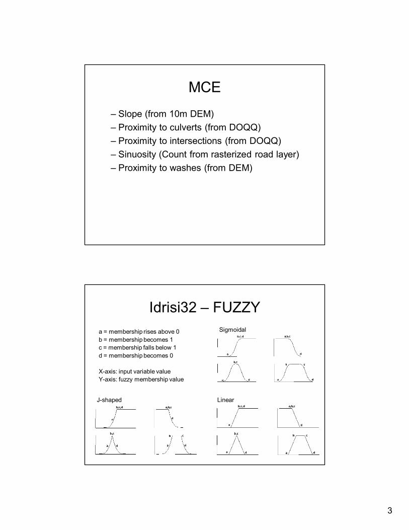
MCE

– Slope (from 10m DEM) – Proximity to culverts (from DOQQ) – Proximity to intersections (from DOQQ) – Sinuosity (Count from rasterized road layer) – Proximity to washes (from DEM)

Idrisi32 – FUZZY a = membership rises above 0 b = membership becomes 1 c = membership falls below 1 d = membership becomes 0

X­axis: input variable value Y­axis: fuzzy membership value

J­shaped Linear

Sigmoidal

4

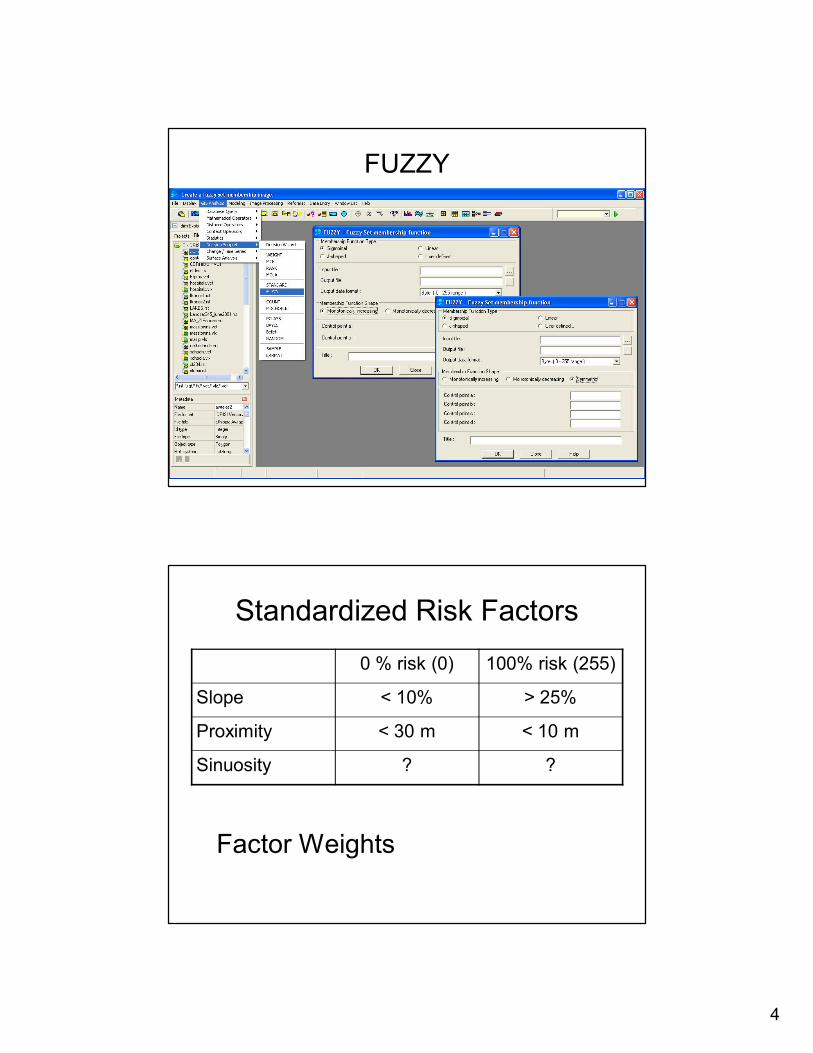
FUZZY

Standardized Risk Factors

0 % risk (0) 100% risk (255)

Slope < 10% > 25%

Proximity < 30 m < 10 m

Sinuosity ? ?

Factor Weights

5

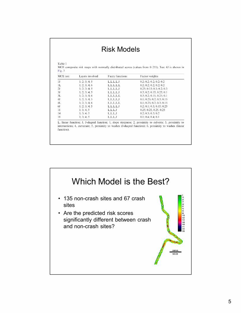
Risk Models

Which Model is the Best?

• 135 non­crash sites and 67 crash sites

• Are the predicted risk scores significantly different between crash and non­crash sites?

6

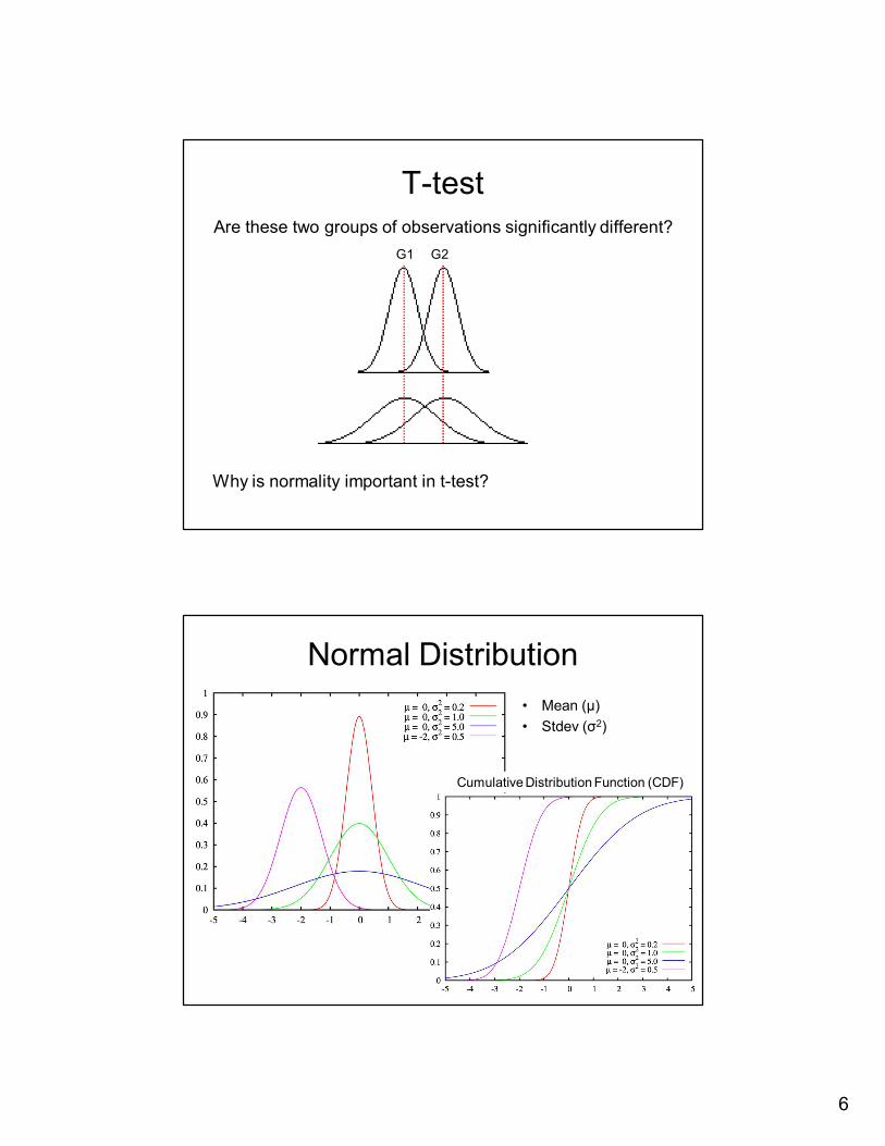
T­test Are these two groups of observations significantly different?

G1 G2

Why is normality important in t­test?

Normal Distribution • Mean (μ) • Stdev (σ 2 )

Cumulative Distribution Function (CDF)

7

Test for Normality • Statistic

– Kolmogorov­Smirnov (K­S) – Lilifors – Shapiro­Wilks

• Visual – DF (histogram) / CDF – Stemplot – QQ Plot

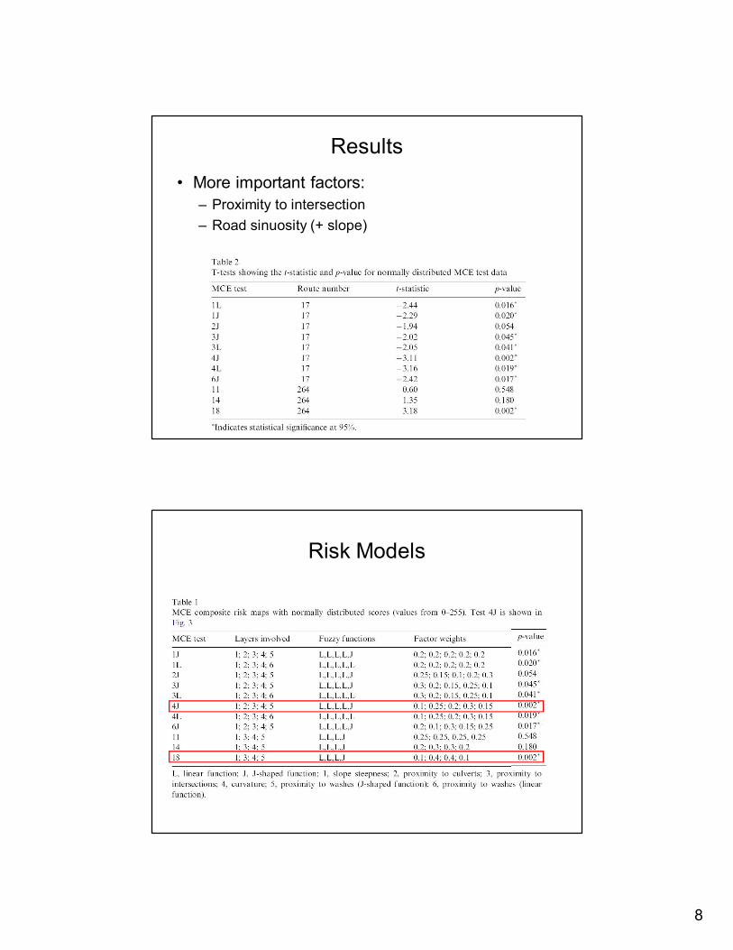
Stem­and­leaf Plot

8

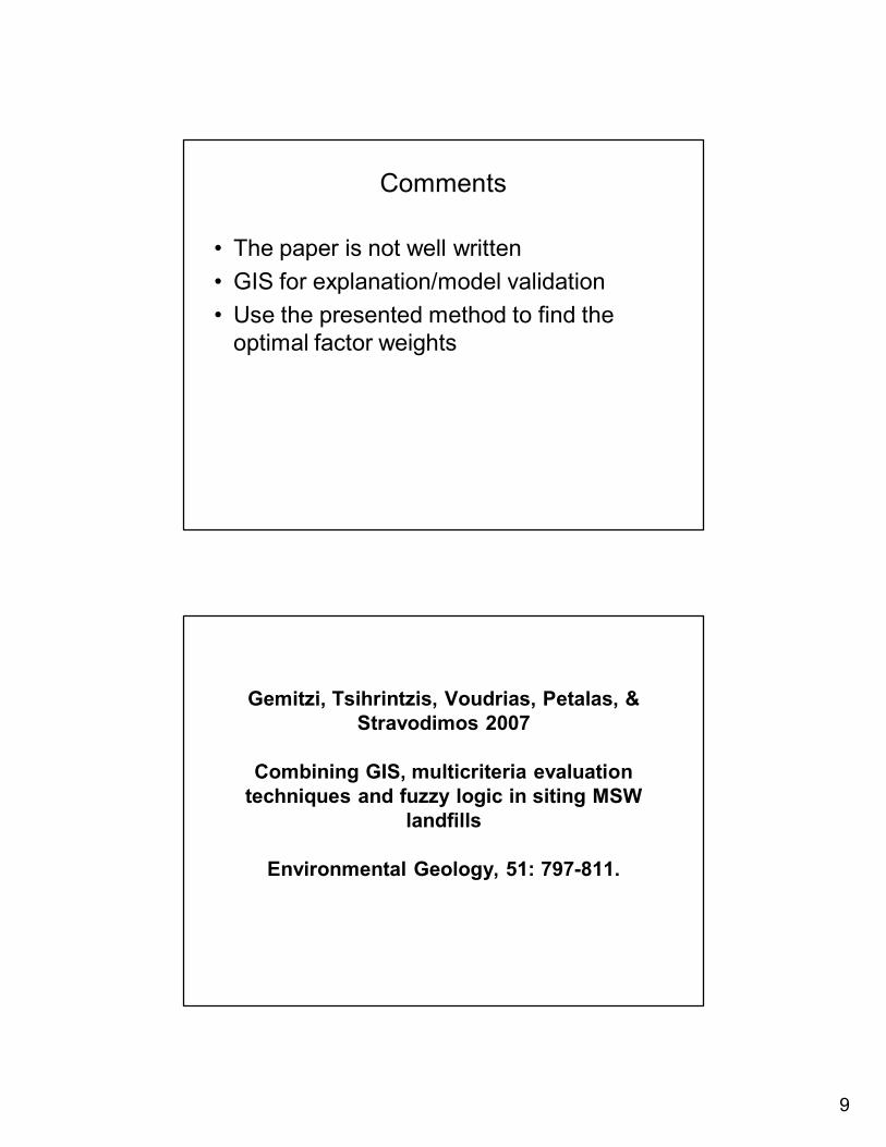
Results • More important factors:

– Proximity to intersection – Road sinuosity (+ slope)

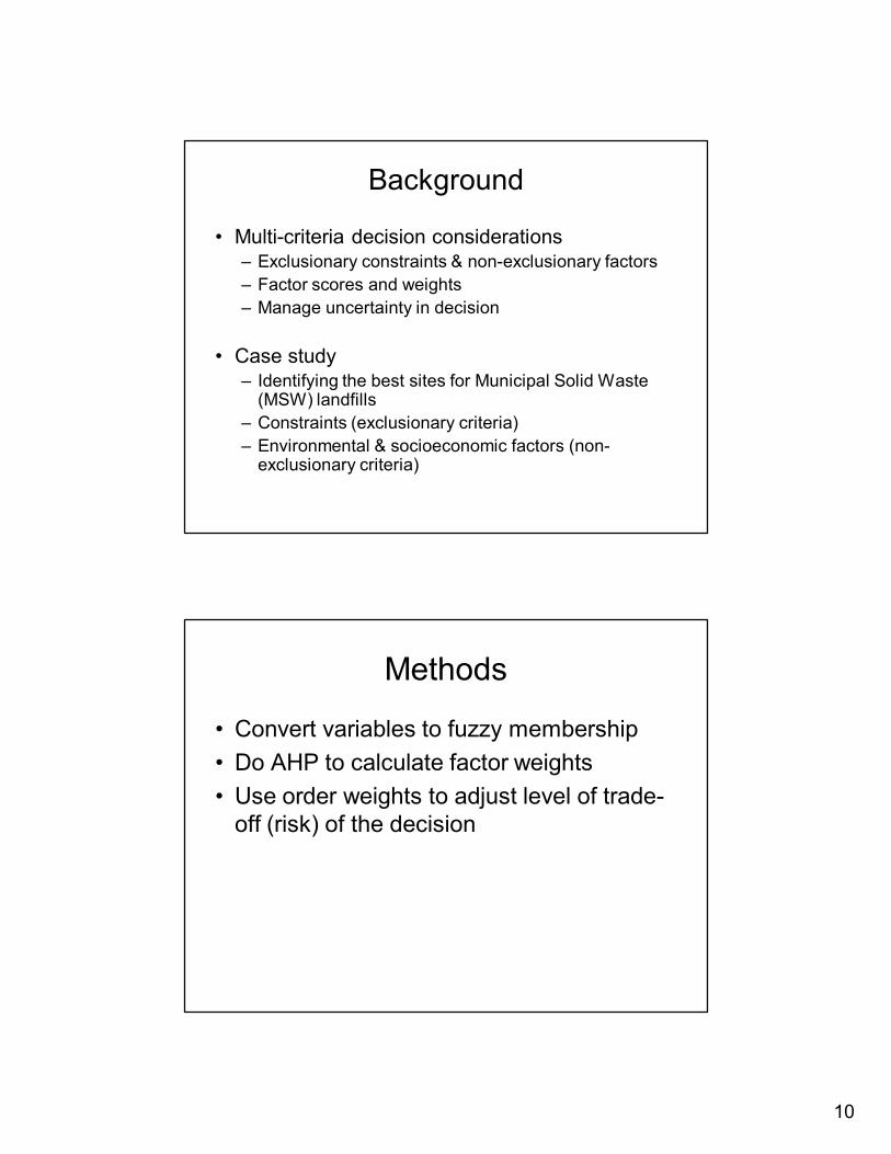
Risk Models

9

Comments

• The paper is not well written • GIS for explanation/model validation • Use the presented method to find the optimal factor weights

Gemitzi, Tsihrintzis, Voudrias, Petalas, & Stravodimos 2007

Combining GIS, multicriteria evaluation techniques and fuzzy logic in siting MSW

landfills

Environmental Geology, 51: 797­811.

10

Background

• Multi­criteria decision considerations – Exclusionary constraints & non­exclusionary factors – Factor scores and weights – Manage uncertainty in decision

• Case study – Identifying the best sites for Municipal Solid Waste (MSW) landfills

– Constraints (exclusionary criteria) – Environmental & socioeconomic factors (non­ exclusionary criteria)

Methods

• Convert variables to fuzzy membership • Do AHP to calculate factor weights • Use order weights to adjust level of trade­ off (risk) of the decision

11

Decision Criteria Constraints

– Residential area – Land uses – Highways & railways – Environmental protected areas – Important aquifers – Surface water bodies – Springs and wells – Exceptional geological conditions – Distance from country borders & coastline

Environmental Factors – Hydrogeology – Hydrology – Distance from water bodies

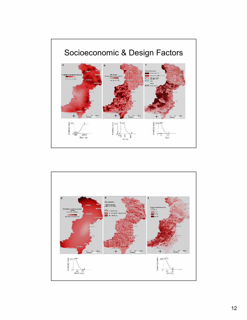
Socioeconomic & design factors – Proximity to residential areas – Site access – Type of land use – Proximity to waste production centers – Site orientation – Slope of land surface

IDRISI FUZZY a = membership rises above 0 b = membership becomes 1 c = membership falls below 1 d = membership becomes 0

12

Socioeconomic & Design Factors

13

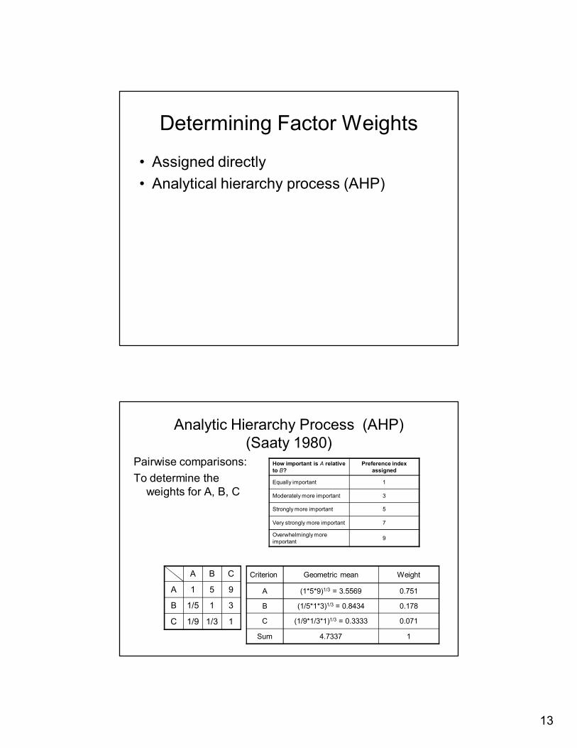
Determining Factor Weights

• Assigned directly • Analytical hierarchy process (AHP)

Analytic Hierarchy Process (AHP) (Saaty 1980)

Pairwise comparisons: To determine the weights for A, B, C

How important is A relative to B?

Preference index assigned

Equally important 1

Moderately more important 3

Strongly more important 5

Very strongly more important 7

Overwhelmingly more important 9

A B C

A 1 5 9

B 1/5 1 3

C 1/9 1/3 1

Criterion Geometric mean Weight

A (1*5*9) 1/3 = 3.5569 0.751

B (1/5*1*3) 1/3 = 0.8434 0.178

C (1/9*1/3*1) 1/3 = 0.3333 0.071

Sum 4.7337 1

14

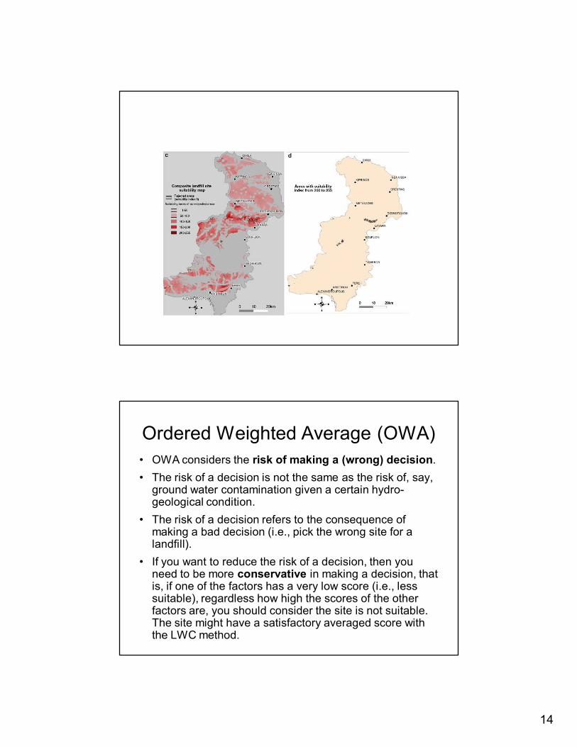
Ordered Weighted Average (OWA) • OWA considers the risk of making a (wrong) decision. • The risk of a decision is not the same as the risk of, say, ground water contamination given a certain hydro­ geological condition.

• The risk of a decision refers to the consequence of making a bad decision (i.e., pick the wrong site for a landfill).

• If you want to reduce the risk of a decision, then you need to be more conservative in making a decision, that is, if one of the factors has a very low score (i.e., less suitable), regardless how high the scores of the other factors are, you should consider the site is not suitable. The site might have a satisfactory averaged score with the LWC method.

15

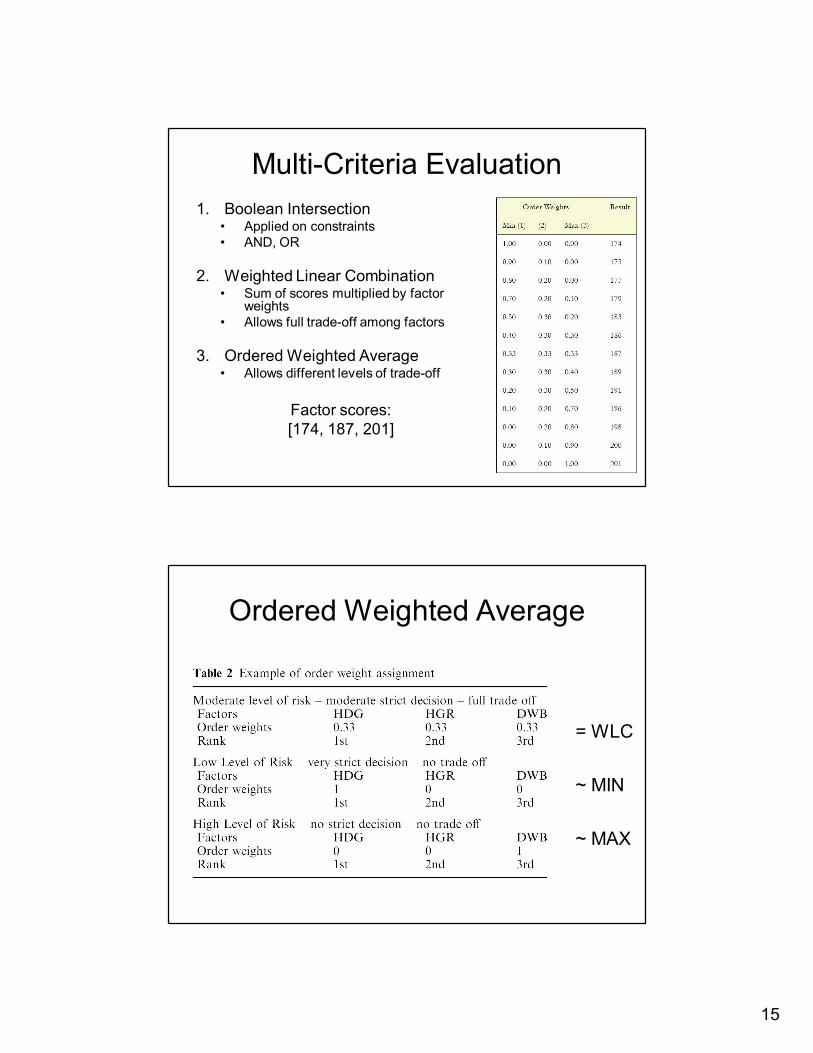
Multi­Criteria Evaluation 1. Boolean Intersection

• Applied on constraints • AND, OR

2. Weighted Linear Combination • Sum of scores multiplied by factor

weights • Allows full trade­off among factors

3. Ordered Weighted Average • Allows different levels of trade­off

Factor scores: [174, 187, 201]

Ordered Weighted Average

= WLC

~ MIN

~ MAX

16

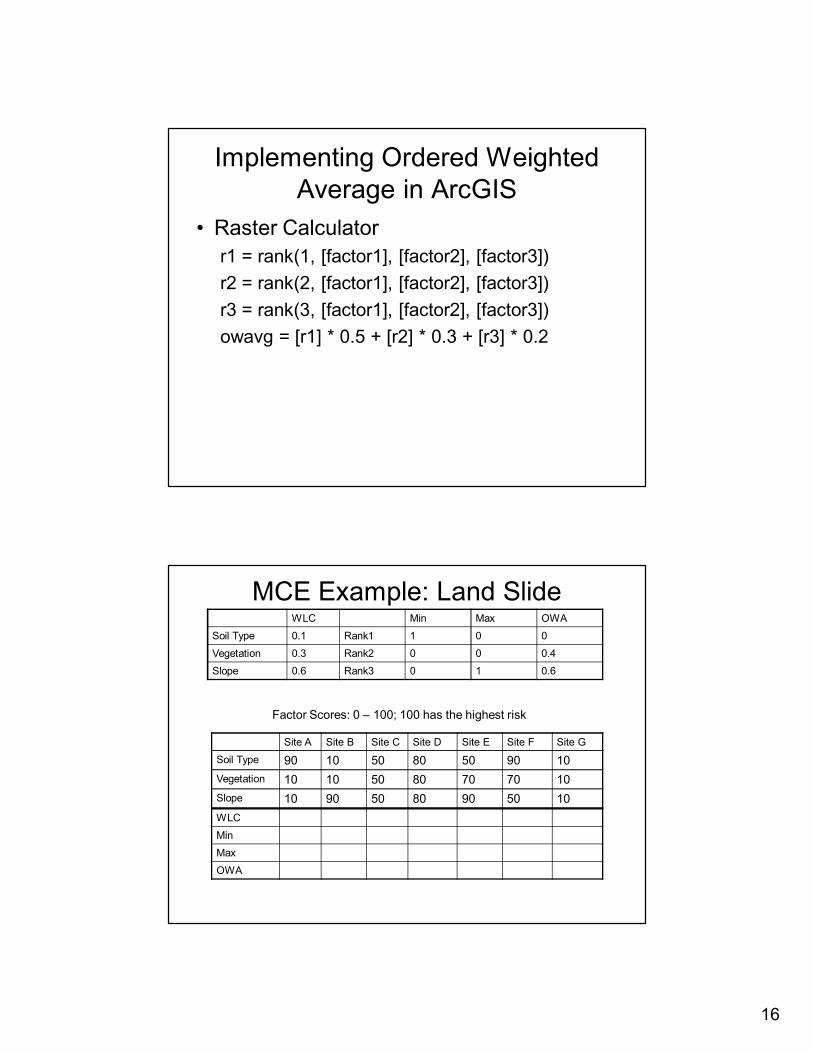
Implementing Ordered Weighted Average in ArcGIS

• Raster Calculator r1 = rank(1, [factor1], [factor2], [factor3]) r2 = rank(2, [factor1], [factor2], [factor3]) r3 = rank(3, [factor1], [factor2], [factor3]) owavg = [r1] * 0.5 + [r2] * 0.3 + [r3] * 0.2

MCE Example: Land Slide

Site A Site B Site C Site D Site E Site F Site G

Soil Type 90 10 50 80 50 90 10 Vegetation 10 10 50 80 70 70 10 Slope 10 90 50 80 90 50 10

WLC Min Max OWA

Soil Type 0.1 Rank1 1 0 0

Vegetation 0.3 Rank2 0 0 0.4

Slope 0.6 Rank3 0 1 0.6

Factor Scores: 0 – 100; 100 has the highest risk

WLC

Min

Max

OWA

17

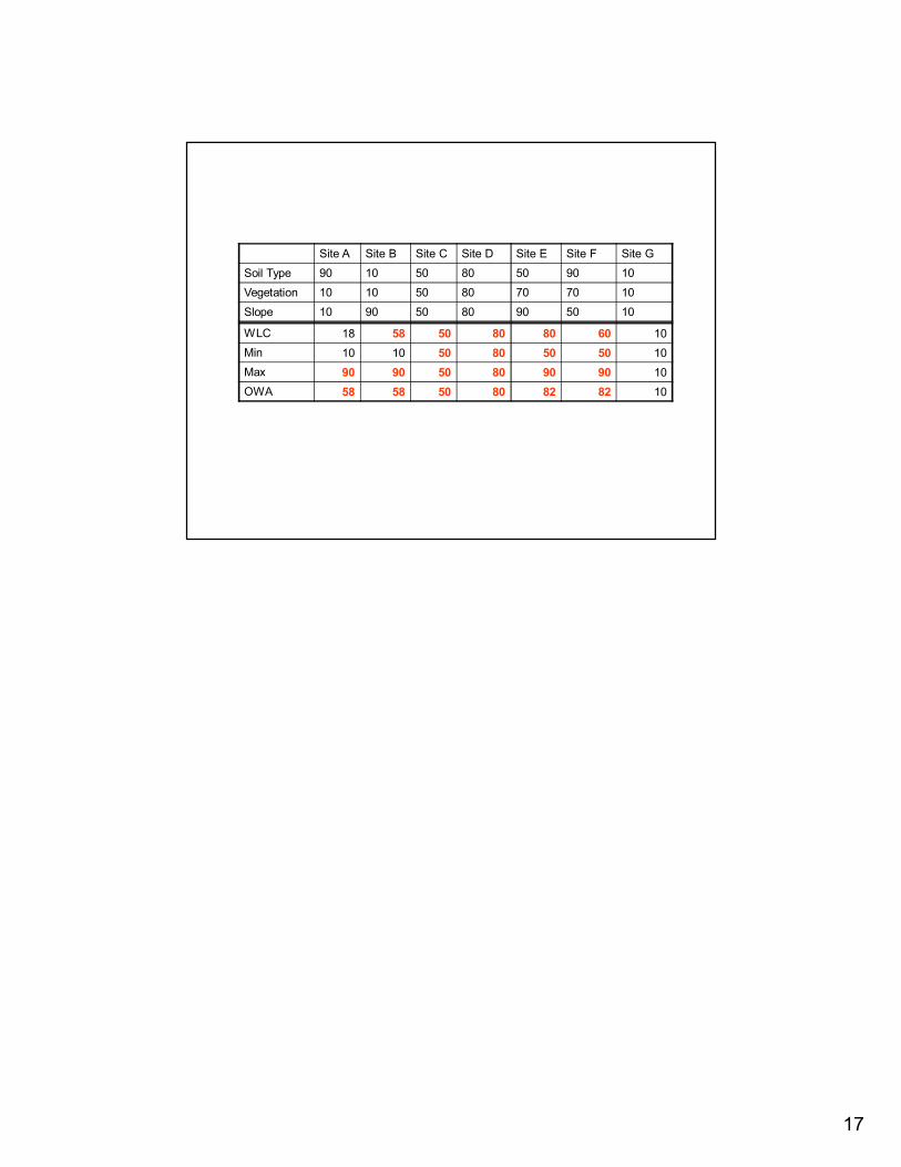
Site A Site B Site C Site D Site E Site F Site G

Soil Type 90 10 50 80 50 90 10

Vegetation 10 10 50 80 70 70 10

Slope 10 90 50 80 90 50 10

WLC 18 58 50 80 80 60 10 Min 10 10 50 80 50 50 10 Max 90 90 50 80 90 90 10 OWA 58 58 50 80 82 82 10