Embed Size (px)
Citation preview

Progress In Electromagnetics Research, PIER 24, 279–310, 1999
FULL-WAVE ANALYSIS OF A FABRY-PEROT TYPE
RESONATOR
D. I. Kaklamani
Department of Electrical and Computer EngineeringNational Technical University of Athens9 Iroon Polytechniou Str.15780 Zografos, Athens, Greece
1. Introduction2. Formulation of the Multi-plate Problem3. Solution Via Entire Domain Galerkin Technique4. Numerical Results5. Conclusions–Future WorkMathematical AppendixReferences
1. INTRODUCTION
The analysis of open resonators consisting of two parallel orthogonalparallelepiped conductors has been among the first to be carried outby computer techniques, approximately 40 years ago [1]. The semi-open nature of the parallel plate resonator eliminates large number ofpossible modes, which would be rapidly damped by the radiation fromthe open sides [2], keeping only longitudinal resonances. This fact hasplayed an essential role in the development of laser systems at opticalfrequencies and the construction of active quantum electronic devices.The system of parallel plate reflectors has been used for very long inthe classical Fabry-Perot interferometer [3] and this is why it is usuallyreferred to as Fabry-Perot resonator. Indeed, Fabry-Perot interferome-ters of a metal-dielectric-metal configuration have been widely used asbandpass optical filters and laser resonators [4–6]. Recently, there hasbeen a continuously increasing interest of using Fabry-Perot structures

280 Kaklamani
as a wavemeter at microwave and millimetre wavelength frequencies[7–10], as well as to determine the material properties of high tem-perature superconductors [11–16]. Similar open type structures areproposed to be used at sub-millimetre wavelengths where, contraryto the optical wavelengths, the resonator dimensions are comparableto the operation wavelengths. In this case, it is required to computethe resonance properties of low order modes in the Fabry-Perot typestructures. The same statements are valid for optical microresonatorswhere, again, low order modes are employed.
In this paper, an open resonator of the type shown in Figure 1(a),consisting of two equal parallel plates and excited by an elementarydipole parallel to the plates, is examined. This structure is directly re-lated to the famous Casimir effect [17, 18], which exhibits the vacuumenergy of the electromagnetic field as a weak attraction force betweentwo uncharged perfectly conducting plates very close to each other.The existence of this force, which is linked with fundamental conceptsof physics, such as virtual particles and zero energy fluctuations, hasrecently re-attracted much interest and was confirmed by a very accu-rately designed experiment by Lamoreaux [19].
The analysed structure shown in Figure 1(a) is derived as a spe-cial case of the Q-number of perfectly conducting parallel rectangularplates—or equivalently the case of Q-number of rectangular apertures“cut” on parallel infinite screens—shown in Figure 1(b). Actually, thismulti-plate problem has been addressed in a series of papers [20–22],by extending the work presented in [23] for a single rectangular con-ducting plate and using High Performance Computing (HPC) merelyas a computational tool to reduce drastically the consumed CPU time.Therefore, according to the pursued analysis, the two plates shown inFigure 1(a) could be displaced and/or not necessarily of the same di-mensions. Furthermore, the pursued analysis can be easily extended tothe case of multi Fabry-Perot resonators, taking into account couplingphenomena between closely spaced resonators.
In section 2, the formulation of the multi-plate problem is presentedand a system of coupled integral equations is derived in terms of theconductivity currents induced on the parallel displaced rectangularconducting plates surfaces. The system of integral equations is solvedin section 3, using a Method of Moments (MoM) and in particular aGalerkin technique. Entire domain Chebyshev type basis functions in-corporating the current edge behaviour [24], which have been proved
Full-wave analysis of a Fabry-Perot type resonator 281
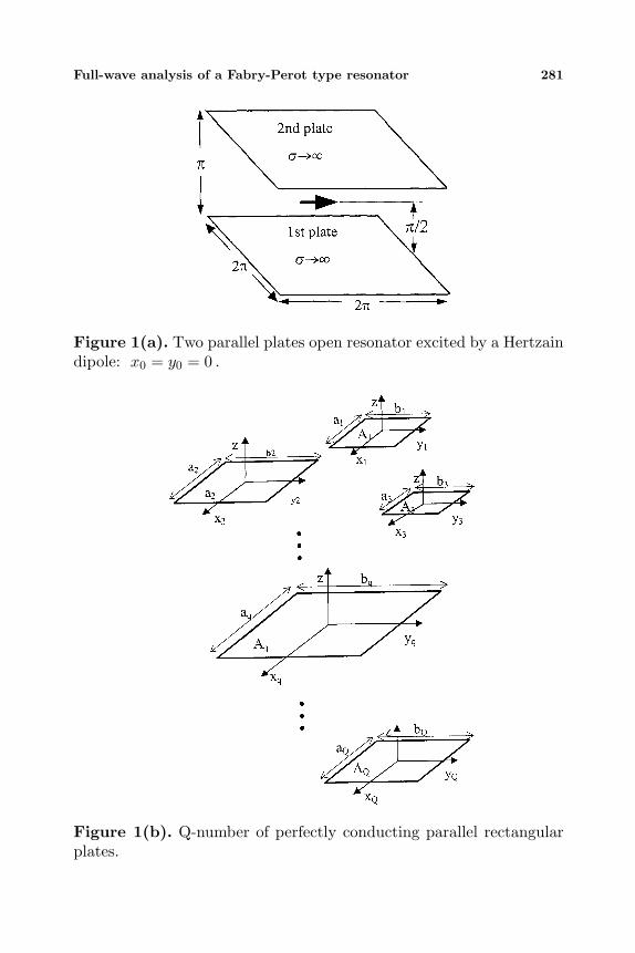
Figure 1(a). Two parallel plates open resonator excited by a Hertzaindipole: x0 = y0 = 0 .
Figure 1(b). Q-number of perfectly conducting parallel rectangularplates.

282 Kaklamani
very efficient in previous works [23, 25], are employed to describe theunknown currents on the plates. Numerical results are presented insection 4 for several resonator sizes and operation frequencies, whileconcluding remarks and topics for further work are given in section 5.
In the following, an exp(jωt) time dependence is assumed and sup-pressed throughout the analysis. The main emphasis is given to near-field quantities, such as the conductivity currents distribution on theplates surface.
2. FORMULATION OF THE INTEGRAL EQUATIONS
The analysis presented in [23] is extended for the case of Q-numberof perfectly conducting infinitesimal thickness plates, placed at arbi-trary positions and orientations on parallel planes—or equivalently thecase of Q-number of rectangular apertures “cut” on parallel infinitescreens—as shown in Figure 1(b), which are illuminated by an exter-nal source with known pattern. For the purpose of the present analysis,the multi-plate structure is illuminated by a primary field
E0(r, r0) = mδ ·G(r, r0) (1)
which is created by a parallel to the xy-plane Hertzian dipole, withorientation vector
δ = cosϕδx + sinϕδy 0 ≤ ϕδ ≤ 2π (2)
position vector
r0 = (x0, y0, δ) −∞ < x0, y0 < +∞ (3)
and electric moment m = I , being the dipole length and I beingthe constant current flowing on the dipole surface. Alternatively, for aplane wave incidence, the primary field is given by
E0(r) = E0e exp(−jk0ki · r) (4)
where e = (cosϕex + sinϕey) sin θe + cos θez and ki = kµixx + kµiyy+kµiz z are the unit vectors denoting the polarisation and incidence direc-tions respectively and E0 is the assumed unit plane wave amplitude.
Applying the Green’s theorem, the electric field is expressed as asummation of the primary excitation E0(r) (Hertzian dipole or plane
Full-wave analysis of a Fabry-Perot type resonator 283
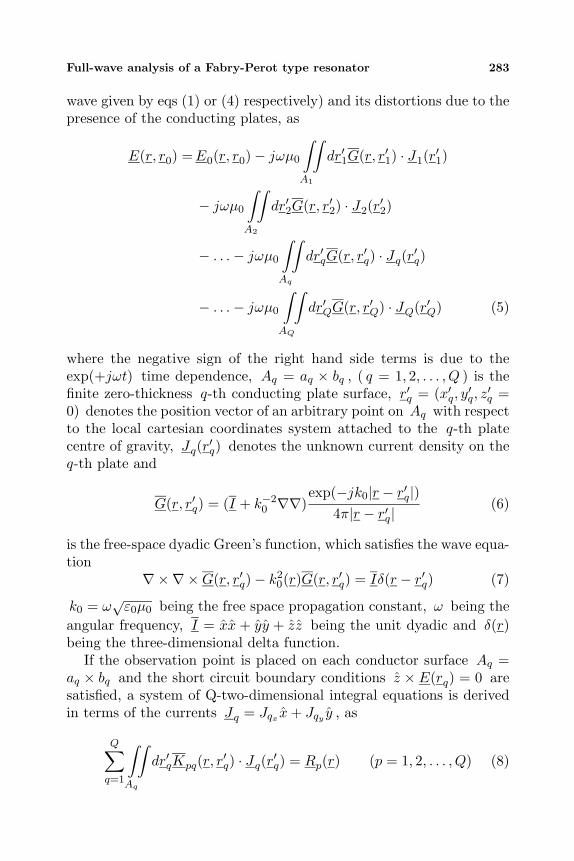
wave given by eqs (1) or (4) respectively) and its distortions due to thepresence of the conducting plates, as
E(r, r0) =E0(r, r0)− jωµ0
∫A1
∫dr′1G(r, r′1) · J1(r
′1)
− jωµ0
∫A2
∫dr′2G(r, r′2) · J2(r
′2)
− . . .− jωµ0
∫Aq
∫dr′qG(r, r′q) · Jq(r′q)
− . . .− jωµ0
∫AQ
∫dr′QG(r, r′Q) · JQ(r′Q) (5)
where the negative sign of the right hand side terms is due to theexp(+jωt) time dependence, Aq = aq × bq , ( q = 1, 2, . . . , Q ) is thefinite zero-thickness q-th conducting plate surface, r′q = (x′q, y
′q, z′q =
0) denotes the position vector of an arbitrary point on Aq with respectto the local cartesian coordinates system attached to the q-th platecentre of gravity, Jq(r′q) denotes the unknown current density on theq-th plate and
G(r, r′q) = (I + k−20 ∇∇)
exp(−jk0|r − r′q|)4π|r − r′q|
(6)
is the free-space dyadic Green’s function, which satisfies the wave equa-tion
∇×∇×G(r, r′q)− k20(r)G(r, r′q) = Iδ(r − r′q) (7)
k0 = ω√ε0µ0 being the free space propagation constant, ω being the
angular frequency, I = xx + yy + zz being the unit dyadic and δ(r)being the three-dimensional delta function.
If the observation point is placed on each conductor surface Aq =aq × bq and the short circuit boundary conditions z × E(rq) = 0 aresatisfied, a system of Q-two-dimensional integral equations is derivedin terms of the currents Jq = Jqx x+ Jqy y , as
Q∑q=1
∫Aq
∫dr′qKpq(r, r
′q) · Jq(r′q) = Rp(r) (p = 1, 2, . . . , Q) (8)

284 Kaklamani
where the subscript q (q = 1, 2, . . . , Q) , wherever used, denotes theq-th plate, Kpq are known kernel matrix functions incorporating thefree-space dyadic Green’s function and the known right hand vectorsRp describe the primary excitation impact. The form of the Kpq
kernel functions depend exclusively on the geometry of the structure(i.e., the dimensions and the relative position of the plates), while theRp right hand functions depend on the type of the external source.
3. SOLUTION VIA ENTIRE DOMAIN GALERKINTECHNIQUE
The system of integral equations (8) is solved by employing an en-tire domain Galerkin technique [26], where the unknown vector quan-tities Jq(r′q) should be expanded in terms of linearly independent“appropriate” basis functions [24–29]. To this end, Chebyshev typeseries with convenient arguments, incorporating the current edge be-haviour, which have been proved very efficient in previous works [23,25], are employed. Therefore, with respect to the local cartesian coor-dinates system (xq, yq) , attached to the q-th plate centre of gravity(q = 1, 2, . . . , Q) , the corresponding transverse conductivity currentsare expressed as
Jqx(rq) = s(xq, yq)Nq∑n=0
Mq∑m=0
cqnmΦqnm(xq, yq)
= s(xq, yq)Nq∑n=0
Mq∑m=0
cqnmUn
(2xqaq
)Tm
(2yqbq
)(9.1)
Jqx(rq) =1
s(xq, yq)
Nq∑n=0
Mq∑m=0
dqnmΞqnm(xq, yq)
=1
s(xq, yq)
Nq∑n=0
Mq∑m=0
dqnmUm
(2yqbq
)Tn
(2xqaq
)(9.2)
where Tn and Un are the n-th order Chebyshev polynomials of thefirst and second kind respectively, whose arguments are chosen in a waythat the appropriate stationary waves are developed on the conductingplates surfaces,
s(xq, yq) =
√1− (2xq/aq)2
1− (2yq/bq)2(q = 1, 2, . . . , Q) (10)
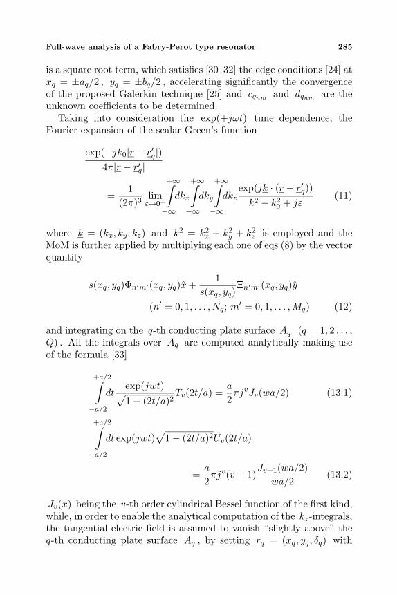
Full-wave analysis of a Fabry-Perot type resonator 285
is a square root term, which satisfies [30–32] the edge conditions [24] atxq = ±aq/2 , yq = ±bq/2 , accelerating significantly the convergenceof the proposed Galerkin technique [25] and cqnm and dqnm are theunknown coefficients to be determined.
Taking into consideration the exp(+jωt) time dependence, theFourier expansion of the scalar Green’s function
exp(−jk0|r − r′q|)4π|r − r′q|
=1
(2π)3limε→0+
+∞∫−∞
dkx
+∞∫−∞
dky
+∞∫−∞
dkzexp(jk · (r − r′q))k2 − k2
0 + jε(11)
where k = (kx, ky, kz) and k2 = k2x + k2
y + k2z is employed and the
MoM is further applied by multiplying each one of eqs (8) by the vectorquantity
s(xq, yq)Φn′m′(xq, yq)x+1
s(xq, yq)Ξn′m′(xq, yq)y
(n′ = 0, 1, . . . , Nq; m′ = 0, 1, . . . ,Mq) (12)
and integrating on the q-th conducting plate surface Aq (q = 1, 2 . . . ,Q) . All the integrals over Aq are computed analytically making useof the formula [33]
+a/2∫−a/2
dtexp(jwt)√1− (2t/a)2
Tv(2t/a) =a
2πjvJv(wa/2) (13.1)
+a/2∫−a/2
dt exp(jwt)√
1− (2t/a)2Uv(2t/a)
=a
2πjv(v + 1)
Jv+1(wa/2)wa/2
(13.2)
Jv(x) being the v-th order cylindrical Bessel function of the first kind,while, in order to enable the analytical computation of the kz-integrals,the tangential electric field is assumed to vanish “slightly above” theq-th conducting plate surface Aq , by setting rq = (xq, yq, δq) with
286 Kaklamani
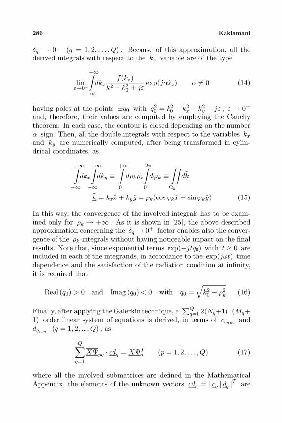
δq → 0+ (q = 1, 2, . . . , Q) . Because of this approximation, all thederived integrals with respect to the kz variable are of the type
limε→0+
+∞∫−∞
dkzf(kz)
k2 − k20 + jε
exp(jαkz) α = 0 (14)
having poles at the points ±q0 with q20 = k20 − k2
x − k2y − jε , ε→ 0+
and, therefore, their values are computed by employing the Cauchytheorem. In each case, the contour is closed depending on the numberα sign. Then, all the double integrals with respect to the variables kxand ky are numerically computed, after being transformed in cylin-drical coordinates, as
+∞∫−∞
dkx
+∞∫−∞
dky ≡+∞∫0
dρkρk
2π∫0
dϕk ≡∫Ωk
∫dk
k = kxx+ kyy = ρk(cosϕkx+ sinϕky) (15)
In this way, the convergence of the involved integrals has to be exam-ined only for ρk → +∞ . As it is shown in [25], the above describedapproximation concerning the δq → 0+ factor enables also the conver-gence of the ρk-integrals without having noticeable impact on the finalresults. Note that, since exponential terms exp(−jtq0) with t ≥ 0 areincluded in each of the integrands, in accordance to the exp(jωt) timedependence and the satisfaction of the radiation condition at infinity,it is required that
Real (q0) > 0 and Imag (q0) < 0 with q0 =√k2
0 − ρ2k (16)
Finally, after applying the Galerkin technique, a∑Q
q=1 2(Nq+1) (Mq+1) order linear system of equations is derived, in terms of cqnm anddqnm (q = 1, 2, ..., Q) , as
Q∑q=1
XΨpq · cdq = XΨ0p (p = 1, 2, . . . , Q) (17)
where all the involved submatrices are defined in the MathematicalAppendix, the elements of the unknown vectors cdq = [ cq | dq ]T are
Full-wave analysis of a Fabry-Perot type resonator 287
the unknown coefficients cqnm and dqnm to be determined and theposition of each submatrice element is defined by transforming thedouble pointers to simple ones. Note that, in all the expressions givenin the Mathematical Appendix, special care has been taken in mak-ing the proper transformations from each local cartesian coordinatessystem attached to the q-th plate centre of gravity —denoted by thesubscript q , as (xq, yq, zq)—to a global cartesian coordinates system—denoted without any subscript, as (x, y, z) , taking into account thatthe position vector of the q-th plate centre of gravity is denoted bythe formula
r0q = x0q x+ y0
q y + z0q z (q = 1, 2, . . . , Q) (18)
with respect to a global system of coordinates (x, y, z) .The successful choice of the entire domain basis functions leads to
quick convergence and small order systems (i.e., small Nq , Mq values).Therefore, the use of indirect methods is not needed and the systemis numerically solved by employing the method of triangulation. Notethat, all the system kernel elements are double integrals of the form∫ +∞0 dρk
∫ 2π0 dϕk given by eq. (15), which refer to the Green’s func-
tion Fourier expansion and are numerically computed, by a 12-pointquadrature Gauss algorithm [33], as in [23, 25]. Once the unknowncoefficients are determined, the currents on the plates surfaces and theelectric field in the near and far field region are computed, using theformula [33]
Tn(cos θ) = cos(nθ) Un(cos θ) = sin[(n+ 1)θ]/ sin θ (19)
4. NUMERICAL RESULTS
Numerical calculations are carried out applying the analysis presentedin the previous two sections. In order to calculate the conductivitycurrents induced on the plates surfaces and given by eqs (9) and (19),the unknown expansion coefficients cqnm and dqnm are determined bynumerically solving the
∑Qq=1 2(Nq + 1)(Mq + 1) order linear system
of equations (17) via the method of triangulation. In calculating thekernel elements and the right hand side elements, all the involved dou-ble integrals
∫∫Ωkdk ≡
∫ +∞0 dρkρk
∫ 2π0 dϕk appearing in eqs (A.1) and
(A.4) of the Mathematical Appendix are numerically computed em-ploying a 12-point quadrature Gauss integration algorithm [33]. The

288 Kaklamani
only singularity point of the integrands is the ρk = k0 branch pointand the proper selection of the branch cut is determined by the sat-isfaction of the radiation conditions at the ρk-complex plane. Then,the convergence of the integrals value is checked with respect to boththe ρk and ϕk subdivisions and the truncation of the ρk-integrationupper limit. The right hand side integrands (A.4) exhibit an expo-nential behavior e−ρksgn(δ−z0p)(δ−z0p−δp) (p = 1, 2, . . . , Q) for ρk → ∞and, therefore, converge very fast, depending on the δ and z0p relativevalues. Then, the approximation that is described in section 3 concern-ing the δq → 0+ (q = 1, 2, . . . , Q) factor enables the convergence ofthe ρk-integrals (A.1) with respect to their upper limit in the regionsϕk = ±ε , π/2 ± ε , π ± ε and 3π/2 ± ε with 0 < ε << 1 , whosesurface becomes noticeable for large values of the ρk-variable. In theseregions, the worst convergence is exhibited, as e−ρkδq . In all the re-sults that are presented in this section, it is assumed that k0δq = 0.02 .Due to this assumption, although the final results (i.e., current distri-butions) are not affected more than 0.5% , the involved ρk-integralscan be truncated at ρk = 500k0 , while an upper limit ρk = 900k0
is required for k0δq = 0.01 . The necessity of a relatively small valuefor the ρk-integration upper limit is also imposed, when consideringthat a further computational cost increase is caused, due to the factthat, all the (A.1) and (A.4) integrands vary more rapidly with the ρkincrease. Therefore, when integrating with respect to the ϕk-variable,more subdivisions must be considered for large ρk values. It shouldalso be noted that, since it has been numerically proved that the con-tribution to the ρk-integrals final value is much more significant at thebeginning of the ρk-integration path, more dense ρk-subdivisions areneeded for 0 ≤ ρk ≤ 20k0 , while these become much more sparse withthe ρk increase.
After having ensured the convergence of the kernel elements andthe right hand side elements of the linear system of equations (17), theconvergence of the proposed method with respect to the system order∑Q
q=1 2(Nq +1)(Mq +1) , namely with respect to the truncation of the(9.1) and (9.2) expansion series (i.e., the Mq and Nq integers) is con-trolled by computing the conductivity current distributions. Probably,this convergence is expected to be accomplished more rapidly, whenelectrically small plates and/or electrically large distances between theplates and the emitting Hertzian dipole —or moreover a plane waveincidence— are considered. The convergence rate of near field quanti-
Full-wave analysis of a Fabry-Perot type resonator 289
(a)
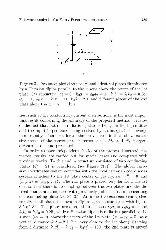
Figure 2. Two uncoupled electrically small identical plates illuminatedby a Hertzian diploe parallel to the x-axis above the centre of the 1stplate: (a) geometry: r01 = 0 , k0a1 = k0a2 = 1 , k0b1 = k0b2 = 0.25 ,ϕδ = 0 , k0x0 = k0y0 = 0 , k0δ = 2.1 and different places of the 2ndplate along the x = y = z line.
ties, such as the conductivity current distributions, is the most impor-tant result concerning the accuracy of the proposed method, becauseof the fact that both the radiation patterns being far field quantitiesand the input impedances being derived by an integration convergemore rapidly. Therefore, for all the derived results that follow, exten-sive checks of the convergence in terms of the Mq and Nq integersare carried out and presented.
In order to have independent checks of the proposed method, nu-merical results are carried out for special cases and compared withprevious works. To this end, a structure consisted of two conductingplates (Q = 2) is considered (see Figure 2(a)). The global carte-sian coordinates system coincides with the local cartesian coordinatessystem attached to the 1st plate centre of gravity, i.e., r01 = 0 and(x, y, z) ≡ (x1, y1, z1) . The 2nd plate is placed very far from the 1stone, so that there is no coupling between the two plates and the de-rived results are compared with previously published data, concerningone conducting plate [23, 34, 35]. An indicative case concerning elec-trically small plates is shown in Figure 2, to be compared with Figure3.5 of [34]. The plates are of equal dimensions k0a1 = k0a2 = 1 andk0b1 = k0b2 = 0.25 , while a Hertzian dipole is radiating parallel to thex-axis (ϕδ = 0) above the centre of the 1st plate (x0 = y0 = 0) at avertical distance k0δ = 2.1 (i.e., very close to the 1st plate). Startingfrom a distance k0x
02 = k0y
02 = k0z
02 = 100 , the 2nd plate is moved
290 Kaklamani
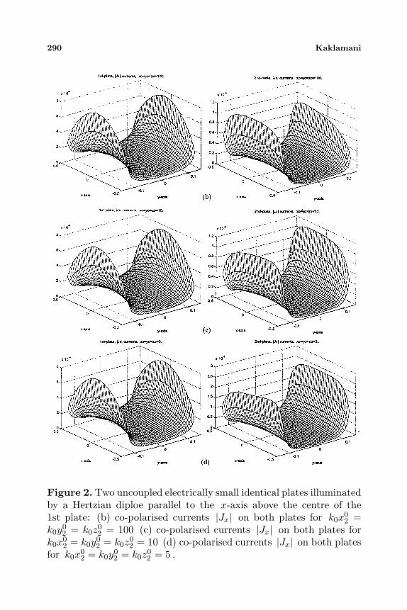
Figure 2. Two uncoupled electrically small identical plates illuminatedby a Hertzian diploe parallel to the x-axis above the centre of the1st plate: (b) co-polarised currents |Jx| on both plates for k0x
02 =
k0y02 = k0z
02 = 100 (c) co-polarised currents |Jx| on both plates for
k0x02 = k0y
02 = k0z
02 = 10 (d) co-polarised currents |Jx| on both plates
for k0x02 = k0y
02 = k0z
02 = 5 .

Full-wave analysis of a Fabry-Perot type resonator 291
towards the 1st one along the x = y = z line (keeping always theprimary source at the same position) and in Figure 2 the co-polarisedcurrents |Jx| induced on both plates are plotted for different placesof the 2nd plate. Due to the electrically small dimensions of bothplates, even for k0x
02 = k0y
02 = k0z
02 = 5 , no coupling between the
two plates is exhibited and the conductivity currents are only affectedby the plates distance from the Hertzian dipole; therefore, only the2nd plate currents alter in Figure 2. In all cases, detailed convergencetest are carried out, which are not presented here. The cross-polarisedcurrents |Jy| converge more slowly than the co-polarised ones |Jx| .Nevertheless, as expected, the cross-polarised currents are one order ofmagnitude smaller than the corresponding co-polarised ones on eachplate, while the currents excited on the 2nd plate start from being alsoone order of magnitude smaller than the corresponding ones induced onthe much closer to the primary source 1st plate and gradually increaseas the 2nd plate approaches the 1st one (and the excitation). The va-lidity of the code is further checked by considering a case symmetricalto the one presented in Figure 2(d). This is done by moving the 2ndplate at k0x0 = k0y0 = 5 and k0δ = 5− 2.1 = 2.9 and getting for the2nd plate the current distributions which corresponded to the 1st platein Figure 2(d) and vise versa. Then, moving to structures like the oneshown in Figure 1(a), the 2nd plate is placed concentrically to the 1stone at k0x
02 = k0y
02 = 0 and k0z
02 = 5 . Nevertheless, the electrically
small dimensions of both plates prevent the structure from behavinglike an open resonator, namely “trapping” part of the radiating energyin-between the two plates region. In order to achieve a resonating be-havior, it is necessary to move to electrically larger dimensions, whichis done in the following. However, dealing with electrically larger struc-tures would lead to practically prohibitive computational cost, both interms of memory requirement and CPU time, since more basis func-tions (i.e., larger Mq and Mq values) would be needed to achieve thesame order of accuracy. This problem is encountered using parallelprocessing techniques, extensively discussed in [20–22].
As already mentioned in the introductory section, the specific caseof two parallel concentric plates (i.e., Q = 2 and (x1, y1) ≡ (x2, y2) ),consisting a Fabry-Perot type open resonator, is of special importance.In Figure 1(a), the specific examined geometry is shown. The openresonator system is excited by a Hertzian dipole placed in the mid-dle of the distance between the two plates ( x0 = y0 = 0 , δ = π/2 ),

292 Kaklamani
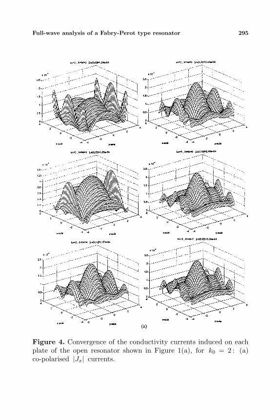
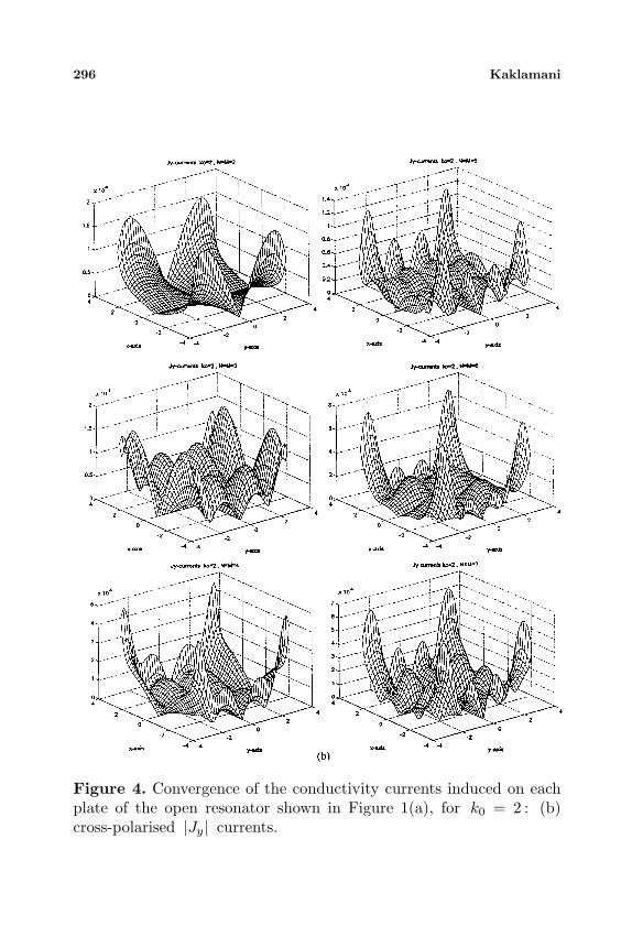
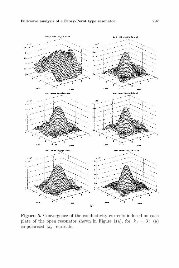
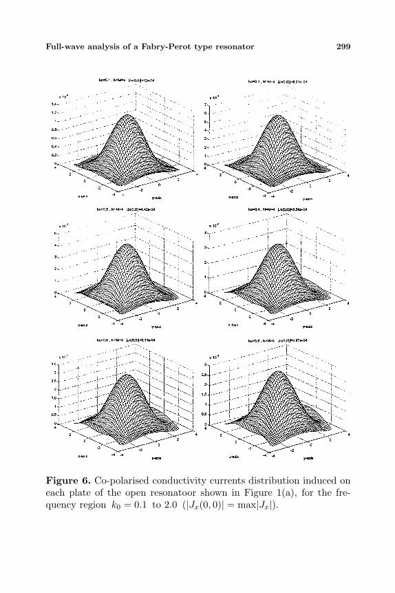
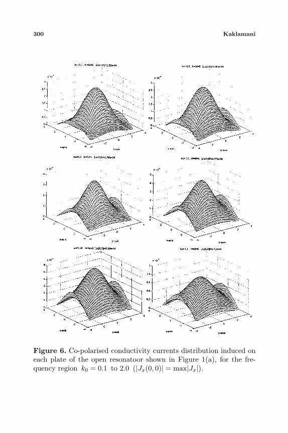
whereas the plates dimensions are aq × bq = 2π × 2π (q = 1, 2) . Dueto the examined structure symmetry, the conductivity currents dis-tribution induced on the two plates surfaces is identical. In order tocompute the system kernel phase space double integrals, the 12-pointquadrature Gauss algorithm is parallelised, by subdividing the integra-tion path and splitting the corresponding calculations on to differentprocessors of the parallel machine. The resulting parallel algorithm iscomputed exhibiting considerable speedups, for plates with dimensionsof multiple wavelengths. Due to the inherent parallel nature of the pro-posed MoM, the results are obtained with minimal additional to thesequential code programming effort [20–23]. Then, the computationtimes become tolerable, allowing for the problem size, hence the accu-racy, to be increased. The numerical results presented in Figures 3–5are performed on a shared-memory Silicon Graphics Power Challengewith 14 TFP processors. The convergence of the conductivity currentdistributions is in any case better than 5% , whereas the convergencerate depends on the problem size, namely the product of the frequencytimes the most critical dimension (plates sizes or dipole-plates dis-tance). This convergence in terms of N1 = N2 = N = M1 = M2 = Mis shown in Figures 3, 4 and 5 for three different operation frequenciesk0 = 1 , 2 and 3 respectively. As expected, the dominant co-polarisedJx currents converge faster than the cross-polarised Jy ones, whichare in any case one order of magnitude smaller. Furthermore, it isclear that, as already mentioned, more basis functions are needed forhigher frequencies. In Figure 6, the resonance behaviour of the exam-ined structure is exhibited by plotting the Jx currents, sweeping thefrequency from k0 = 0.1 to k0 = 2 (with more detailed presentationaround the resonance region k0 = 1 ), while Figure 7 summarises theopen resonator results for the same frequency region.

Full-wave analysis of a Fabry-Perot type resonator 293
Figure 3. Convergence of the conductivity currents induced on eachplate of the open resonator shown in Figure 1(a), for k0 = 1 : (a)co-polarised |Jx| currents.

294 Kaklamani
Figure 3. Convergence of the conductivity currents induced on eachplate of the open resonator shown in Figure 1(a), for k0 = 1 : (b)cross-polarised |Jy| currents.
Full-wave analysis of a Fabry-Perot type resonator 295
Figure 4. Convergence of the conductivity currents induced on eachplate of the open resonator shown in Figure 1(a), for k0 = 2 : (a)co-polarised |Jx| currents.
296 Kaklamani
Figure 4. Convergence of the conductivity currents induced on eachplate of the open resonator shown in Figure 1(a), for k0 = 2 : (b)cross-polarised |Jy| currents.
Full-wave analysis of a Fabry-Perot type resonator 297
Figure 5. Convergence of the conductivity currents induced on eachplate of the open resonator shown in Figure 1(a), for k0 = 3 : (a)co-polarised |Jx| currents.

298 Kaklamani
Figure 5. Convergence of the conductivity currents induced on eachplate of the open resonator shown in Figure 1(a), for k0 = 3 : (b)cross-polarised |Jy| currents.
Full-wave analysis of a Fabry-Perot type resonator 299
Figure 6. Co-polarised conductivity currents distribution induced oneach plate of the open resonatoor shown in Figure 1(a), for the fre-quency region k0 = 0.1 to 2.0 (|Jx(0, 0)| = max|Jx|).
300 Kaklamani
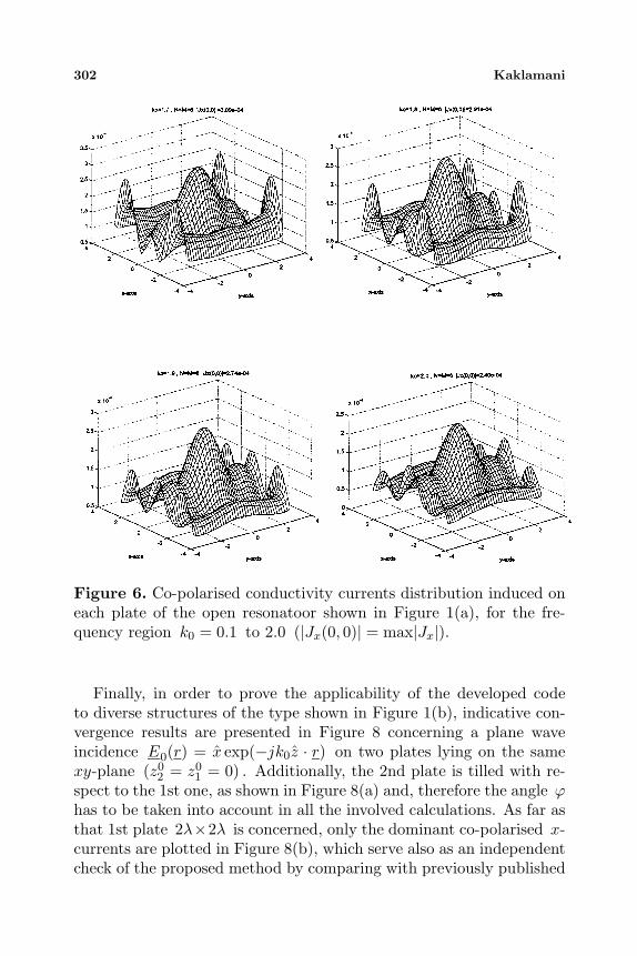
Figure 6. Co-polarised conductivity currents distribution induced oneach plate of the open resonatoor shown in Figure 1(a), for the fre-quency region k0 = 0.1 to 2.0 (|Jx(0, 0)| = max|Jx|).

Full-wave analysis of a Fabry-Perot type resonator 301
Figure 6. Co-polarised conductivity currents distribution induced oneach plate of the open resonatoor shown in Figure 1(a), for the fre-quency region k0 = 0.1 to 2.0 (|Jx(0, 0)| = max|Jx|).
302 Kaklamani
Figure 6. Co-polarised conductivity currents distribution induced oneach plate of the open resonatoor shown in Figure 1(a), for the fre-quency region k0 = 0.1 to 2.0 (|Jx(0, 0)| = max|Jx|).
Finally, in order to prove the applicability of the developed codeto diverse structures of the type shown in Figure 1(b), indicative con-vergence results are presented in Figure 8 concerning a plane waveincidence E0(r) = x exp(−jk0z · r) on two plates lying on the samexy-plane (z02 = z01 = 0) . Additionally, the 2nd plate is tilled with re-spect to the 1st one, as shown in Figure 8(a) and, therefore the angle ϕhas to be taken into account in all the involved calculations. As far asthat 1st plate 2λ×2λ is concerned, only the dominant co-polarised x-currents are plotted in Figure 8(b), which serve also as an independentcheck of the proposed method by comparing with previously published

Full-wave analysis of a Fabry-Perot type resonator 303
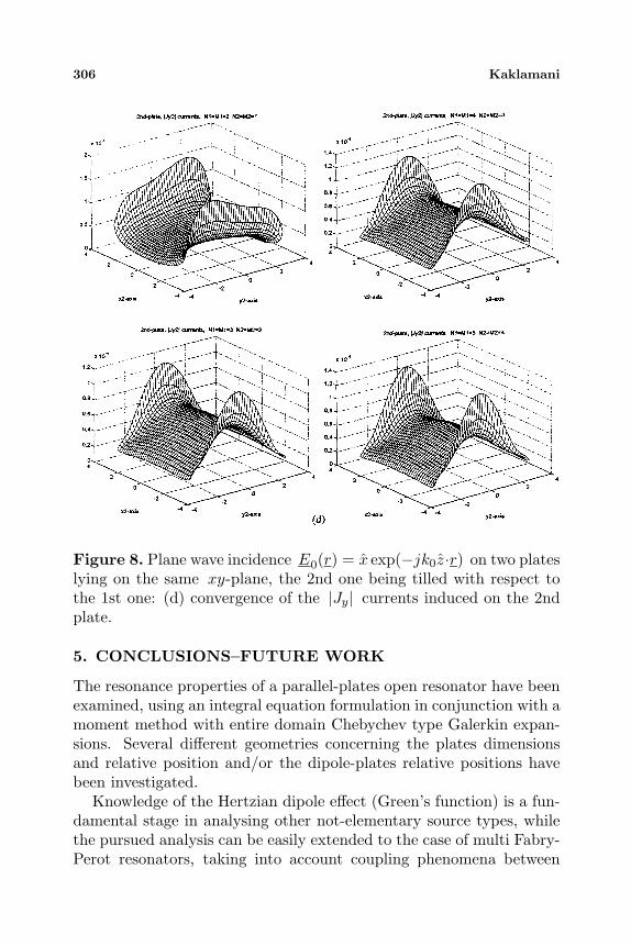
data [23, 35], while as far as the 2nd plate λ×λ is concerned, both x-and y- currents are significant due to the ϕ angle and their conver-gence is exhibited in Figures 8(c) and (d) respectively. Note that, thelatter current distributions on the 2nd plate are plotted with respectto the local cartesian coordinates system (x2, y2) , attached to the 2ndplate centre of gravity.
Figure 7. Max |Jx| distribution in the frequency region k0 = 0.1 to2.0 for the open resonator shown in Figure 1(a).

304 Kaklamani
(a)
Figure 8. Plane wave incidence E0(r) = x exp(−jk0z·r) on two plateslying on the same xy-plane, the 2nd one being tilled with respect tothe 1st one: (a) geometry: z02 = z01 = 0 , x0
2 = y02 = 2λ , a1 = b1 = 2λ ,
a2 = b2 = λ , ϕ = 45o (b) convergence of the |Jx| currents inducedon the 1st plate.

Full-wave analysis of a Fabry-Perot type resonator 305
Figure 8. Plane wave incidence E0(r) = x exp(−jk0z·r) on two plateslying on the same xy-plane, the 2nd one being tilled with respect tothe 1st one: (c) convergence of the |Jx| currents induced on the 2ndplate,
306 Kaklamani
Figure 8. Plane wave incidence E0(r) = x exp(−jk0z·r) on two plateslying on the same xy-plane, the 2nd one being tilled with respect tothe 1st one: (d) convergence of the |Jy| currents induced on the 2ndplate.
5. CONCLUSIONS–FUTURE WORK
The resonance properties of a parallel-plates open resonator have beenexamined, using an integral equation formulation in conjunction with amoment method with entire domain Chebychev type Galerkin expan-sions. Several different geometries concerning the plates dimensionsand relative position and/or the dipole-plates relative positions havebeen investigated.
Knowledge of the Hertzian dipole effect (Green’s function) is a fun-damental stage in analysing other not-elementary source types, whilethe pursued analysis can be easily extended to the case of multi Fabry-Perot resonators, taking into account coupling phenomena between

Full-wave analysis of a Fabry-Perot type resonator 307
closely spaced resonators. Furthermore, once the multi-plate prob-lem shown in Figure 1(b) is solved, more complex conducting struc-tures could be constructed. To this end, other shapes such as rhombs,trapezoids or polygonals will be additionally examined in the future,together with the “corner” problem, in order to construct more com-plicated —in terms of geometry— configurations.
MATHEMATICAL APPENDIX
The analytical expressions of the system (17) kernel elements aredefined as
XΨpq(n,m, n′,m′)
=ωµ0
8π2k20
∫Ωk
∫dke−j[q0sgn(z0p−z0q)(z0p−z0q+δp)+kx(x0
q−x0p)+ky(y
0q−y0p)]
q0
Upn′m′ (−k) ·A(k) · U qnm(k) (A.1)
where ( q = 1, 2, . . . , Q ; p = 1, 2, . . . , Q ), r0q = x0q x+y0
q y+z0q z denotes
the position vector of the q-th plate centre of gravity with respect toa global system of coordinates (x, y, z) , δp → 0+ , k and q0 = q0(k)are defined by eqs (15) and (16) respectively,
U qnm(k) =(n+ 1)Jn+1(−kxaq
2 )Jm(−kybq2 )
2j(n+m)kx/(bqπ2)xx+
(m+ 1)Jm+1(−kybq2 )Jm(−kxaq
2 )2j(n+m)ky/(aqπ2)
yy (A.2)
and
A(k) = A(ρk, φk)= (k2
0 − k2x)xx− kxky(xy + yx) + (k2
0 − k2y)yy (A.3)
As far as the right hand side of eq. (17) is concerned, if the excitationconsists of an elementary horizontal Hertzian dipole defined by eqs(1)–(3), it is valid that
XΨ0p(n′m′)
= − j
8π2k20
∫Ωk
∫dke−j[q0sgn(δ−z0p)(δ−z0p−δp)+ρk(r0·δ)]
q0
R(k) · Upn′m′ (−k) (A.4)
308 Kaklamani
where R(k) = k20 δ − (k · δ)k , while, if a plane wave defined by eq. (4)
illuminates the multi-plate conducting structure, it is valid that
XΨ0p(n′m′) = e exp
[−jk0ki · (r0p + δpz)
]·Upn′m′ (k0ki) (A.5)
ACKNOWLEDGMENT
The author would like to thank Mr. Konstantinos Adam for his assis-tance in obtaining the numerical results presented in Figures 2–8.
REFERENCES
1. Fox, A. G., and T. Li, “Resonant modes in a maser interferome-ter,” Bell Syst. Tech. Jour., Vol. 40, 453–458, March 1961.
2. Schawlow, A. L., and C. H. Townes, “Infrared and optical masers,”Phys. Rev., Vol. 112, 1940–1949, Dec. 1958.
3. Jenkins, F. A., and H. E. White, Fundamentals of Optics, 3rded., McGraw-Hill, New York, 1957.
4. Wait, J. R., Electromagnetic Waves in Stratified Media, Perga-mon Press, New York, 1962.
5. Born, M., and E. Wolf, Principles of Optics, 6th ed., PergamonPress, Oxford, 1980.
6. Haus, H. A., Waves and Fields in Optoelectronics, Prentice-Hall,Inc., Englewood Cliffs, New Jersey, 1984.
7. McCleary, J., M. -Y. Li, and K. Chang, “Ka-band slot-fed higherorder mode low-loss Fabry-Perot filters,” IEEE Trans. Micro-wave Theory Tech., Vol. MTT-42, 1423–1426, July 1994.
8. Sanagi, M., E. Yamamoto, S. Nogi, and R. G. Ranson, “Axi-ally symmetric Fabry-Perot power combiner with active devicesmounted on both the mirrors,” IEEE MTT–S Digest, 1259–1262,17–21 June 1996.
9. Dryagin, Y. A., V. V. Parshin, A. F. Krupnov, N. Gopalsami,and A. C. Raptis, “Precision broadband wavemeter for millimeterand submillimeter range,” IEEE Trans. Microwave Theory Tech.,Vol. MTT-44, 1610–1613, Sept. 1996.
10. Fujii, T., H. Mazaki, F. Takei, J. Bae, M. Narihiro, T. Noda,H. Sakaki, K. Mizuno, and R. G. Ranson, “Coherent power com-bining of millimeter wave resonant tunneling diodes in a quasi-optical resonator,” IEEE MTT-S Digest, 919–922, 17–21 June1996.
11. De Melo, M. T., M. J. Lancaster, H. Yokota, and C. E. Gough,“High temperature superconducting microstrip resonators for the
Full-wave analysis of a Fabry-Perot type resonator 309
measurement of films made by pyrolysis,” Proc. 1995SBMO/IEEE MTT-S, 868–872, 24–27 July 1995.
12. Mourachkine, A. P., and A. R. F. Barel, “Microwave measure-ment of surface resistance by the parallel-plate dielectric res-onator method,” IEEE Trans. Microwave Theory Tech., Vol.MTT-43, 544–551, March 1995.
13. Gevorgian, S., E. Carlsson, P. Linner, E. Kollberg, O. Vendik,and E. Wikborg, “Lower order modes of YBCO/STO/YBCOcircular disk resonators,” IEEE Trans. Microwave Theory Tech.,Vol. MTT-44, 1738–1741, Oct. 1996.
14. Feng, G., M. V. Klein, J. Kruse, and M. Feng, “Mode couplingin superconducting parallel plate resonator in a cavity with outerconductive enclosure,” IEEE Trans. Microwave Theory Tech.,Vol. MTT-44, 944–952, June 1996.
15. Farber, E., G. Deutscher, G. Koren, and E. Jerby, “Microwavemeasurements of high Tc superconductors,” 1996 9th Conv. Elec-trical and Electronics Eng. in Israel, 444–447, 5–6 Nov. 1996.
16. Roan, G. T., and K. A. Zaki, “Calculation of losses in a super-conductive resonator using FDTD,” IEEE AP-S Digest, 384–387,13–18 July 1997.
17. Casimir, H. B. G., and D. Polder, “The influence of retardation onthe London — van den Waals Forces,” Physical Review, Vol. 73,360–372, 1948.
18. Casimir, H. B. G., “On the attraction between two perfectly con-ducting plates,” Proc. Kon. Ned. Akad. Wetensch B51, Vol. 60,793, 1948.
19. Lamoreaux, S. K., “Demonstration of the Casimir Force in the0.6 to 6 µm range,” Physical Review Letters, Vol. 78, No. 1, 5–8,1997, and “Erratum: Demonstration of the Casimir Force in the0.6 to 6 µm range,” Physical Review Letters, Vol. 81, No. 24,5475–5476, 1998.
20. Kaklamani, D. I., and A. Marsh, “Benchmarking high perfor-mance computing platforms in analyzing electrically large pla-nar conducting structures via a parallel computed Method ofMoments technique,” Radio Sci., Vol. 31, 1281–1290, Sept. –Oct. 1996.
21. Kaklamani, D. I., K. S. Nikita, and A. Marsh, “Extension ofmethod of moments for electrical large structures based on paral-lel computations,” IEEE Trans. Antennas Propagat., Vol. AP-45,566–568, March 1997.
22. Marsh, A., D. I. Kaklamani, and K. Adam, “Using parallel pro-cessing as a computational tool to solve multi-plate electromag-netic scattering problems,” accepted for publication in Parallel

310 Kaklamani
Processing Letters.23. Kaklamani, D. I., and A. Marsh, “Solution of electrically large
planar scattering problems using parallel computed method ofmoments technique,” J. Electro. Waves Applic., Vol. 9, 1313–1337, 1995.
24. Meixner, J., “The behavior of electromagnetic fields at edges,”IEEE Trans. Antennas Propagat., Vol. AP-20, 442–446, 1972.
25. Kaklamani, D. I., and N. K. Uzunoglu, “Scattering from a con-ductive rectangular plate covered by a thick dielectric layer andexcited from a dipole or a plane wave,” IEEE Trans. AntennasPropagat., Vol. AP-42, 1065–1076, 1994.
26. Harrington, R. F., Field Computation by Moment Methods, NewYork: Macmillan, Florida: Krieger Publishing, 1983.
27. Sarkar, T. K., A. R. Djordjevic, and E. Arvas, “On the choice ofexpansion and weighting functions in the numerical solution ofoperator equations,” IEEE Trans. Antennas Propagat., Vol. AP-33, 988–996,1985.
28. Aksun, M. I., and R. Mittra, “Choices of expansion and testingfunctions for the Method of Moments applied to a class of elec-tromagnetic problems,” IEEE Trans. Microwave Theory Tech.,Vol. MTT-41, 503–509, 1993.
29. Coen, G., N. Fache, and D. De Zutter, “Comparison between twosets of basis functions for the current modelling in the galerkinspectral domain solution for microstrips,” IEEE Trans. Micro-wave Theory Tech., Vol. MTT-42, 505–513, 1994.
30. Alanen, E., “Pyramidal and entire domain basis functions in themethod of moments,” J. Electro. Waves Applic., Vol. 5, 315–329,1991.
31. Pozar, D. M., “A reciprocity method of analysis for printed slotand slot-coupled microstrip antennas,” IEEE Trans. AntennasPropagat., Vol. AP-34, 1439–1446, 1989.
32. Sarkar, T. K., S. M. Rao, and A. R. Djordjevic, “Electromagneticscattering and radiation from finite microstrip structures,” IEEETrans. Antennas Propagat., Vol. AP-38, 568–1575, 1990.
33. Abramowitz, M., and I. A. Stegun, Handbook of MathematicalFunctions, Dover Publications, Inc., New York, 1970.
34. Kaklamani, D. I., “Analysis of dielectric-loaded radiation struc-tures,” Ph.D. Dissertation, National Technical University ofAthens, Athens, 1992 (in Greek).
35. Volakis, J. L., and K. Barkeshli, “Applications of the conjugategradient method to radiation and scattering,” Application of Iter-ative Methods to Electromagnetics and Signal Processing, Ch. 4,ed. K. Sarkar, Elsevier Science Publishing Co., 1991.