Working Paper Series

#2007-007 The Behavior of the Maximum Likelihood Estimator of Dynamic

Panel Data Sample Selection Models

Wladimir Raymond, Pierre Mohnen, Franz Palm & Sybrand Schim van der Loeff

United Nations University - Maastricht Economic and social Research and training centre on Innovation and Technology

Keizer Karelplein 19, 6211 TC Maastricht, The Netherlands Tel: (31) (43) 388 4400, Fax: (31) (43) 388 4499, e-mail: info@merit.unu.edu, URL: http://www.merit.unu.edu

The Behavior of the Maximum Likelihood Estimator of Dynamic Panel Data Sample Selection Models2

Wladimir Raymond3, Pierre Mohnen4 , Franz Palm5 and Sybrand Schim van der Loeff 6

Abstract This paper proposes a method to implement maximum likelihood estimation of the dynamic panel data type 2 and 3 tobit models. The likelihood function involves a two-dimensional indefinite integral evaluated using “two-step” Gauss-Hermite quadrature. A Monte Carlo study shows that the quadrature works well in finite sample for a number of evaluation points as small as two. Incorrectly ignoring the individual effects, or the dependence between the initial conditions and the individual effects results in an overestimation of the coefficients of the lagged dependent variables. An application to incremental and radical product innovations by Dutch business firms illustrates the method. Keywords: panel data, maximum likelihood estimator, dynamic models, sample selection JEL classification: C33, C34, O31

UNU-MERIT Working Papers ISSN 1871-9872

Maastricht Economic and social Research and training centre on Innovation and Technology,

UNU-MERIT

UNU-MERIT Working Papers intend to disseminate preliminary results of research carried

out at the Centre to stimulate discussion on the issues raised.

2Acknowledgements: The empirical part of this study has been carried out at the Centre for Research of Economic Microdata at Statistics Netherlands. The authors wish to thank Statistics Netherlands, and in particular Bert Diederen, for helping them in accessing and using the Micronoom data set. They wish to thank François Laisney for his helpful comments. The first author acknowledges the financial support from METEOR. 3University of Maastricht, W.Raymond@KE.unimaas.nl 4University of Maastricht, MERIT and CIRANO, MERIT, University of Maastricht, P.O. Box 616 6200 MD Maastricht, The Netherlands; Tel: +31 43 388 3869; Fax: + 31 43 388 4905; P.Mohnen@MERIT.unimaas.nl 5University of Maastricht and CESifo fellow, F.Palm@KE.unimaas.nl 6University of Maastricht, S.Loeff@KE.unimaas.nl

1 Introduction

The ongoing development of the relevant econometric methodology for panel data has increased the

choice for the applied researcher as to which model to choose in any given situation. Whereas this

choice should be driven by the question which underlying assumptions are appropriate in the case

at hand, optimality properties of the estimators are typically known only for large sample sizes. In

order to have some guidance in the choice process it is important to know the implications, in terms

of ease of computation, finite sample properties and the robustness to deviations of the assumptions,

of employing a particular method. In this paper the behavior of the maximum likelihood (ML)

estimator is investigated by means of Monte Carlo simulations in a general model that encompasses

a wide set of models that have been considered in the literature. The generic form of the model

consists of a regression equation, henceforth referred to as the equation of interest, and a selection

equation. Both equations contain a lagged dependent variable and unobserved individual effects

possibly correlated with the explanatory variables. The selection rule may be of the binary type

or of the censoring type.1 In terms of the Amemiya (1984) typology, the models considered in this

paper are the dynamic panel data extensions of the type 2 and type 3 tobit models.2 Variants of

these types of models have been widely used, mostly in labor economics but also in other areas,

but only in a static or “partial” dynamic framework (see Table 1).

This study contributes to the existing literature in a number of ways. Firstly, a practical

method is provided to implement maximum likelihood estimation of the parameters of a panel

sample selection model in which random individual effects and the lagged dependent variable

are included in the equation of interest as well as in the selection equation. The selection rule

may be either of the binary or of the censoring type.3 To handle the initial conditions problem,

Wooldridge’s (2005) solution to this problem in single equation dynamic nonlinear panel data

models is extended to models containing more than one equation. Gaussian quadrature is used

to evaluate the resulting two-dimensional indefinite integral. Secondly, the paper reports on a

Monte Carlo investigation into the behavior in finite samples of the proposed method. It is shown

that using Wooldridge’s solution to deal with the dependence between the initial conditions and

the individual effects is successful in recovering the parameters of a process that generates the

data according to a stationary process. For the likelihood functions generated in the Monte Carlo1Following the literature the term censoring model will be used throughout the paper although it would, in

line with Wooldridge (2005), be preferable to speak of corner solution models since the lagged dependent variableconsidered in this paper is the observed - rather than the latent - variable.

2The type 3 tobit differs from the type 2 tobit in that the selection into the sample is made through a censored(partially continuous) variable instead of a binary variable. The former model uses more information to estimatethe equation of interest than the latter. Hence, we should expect the estimation of the equation of interest to bemore accurate in the former model than in the latter.

3These are the types of selection rule that are mostly considered in the literature (see Table 1). Other types ofselection rule are ordered, multinomial, and those based on multiple indices (Vella, 1998).

1

experiments, Gaussian quadrature, implemented as two successive Gauss-Hermite approximations,

works well for a number of evaluation points as small as two.4 Evidently, when using real data

more than two evaluation points may be necessary to attain the required numerical accuracy.

Nevertheless, the Monte Carlo results indicate that ML estimation of the parameters in a random-

effects dynamic sample selection model is feasible and could conceivably be incorporated as a

command in a general use software package such as Stata. Thirdly, the sensitivity of the ML

estimator to misspecification is also investigated. It is shown that incorrectly ignoring the individual

effects, or the dependence between the initial conditions and the individual effects results in an

overestimation of the coefficients of the lagged dependent variable in both equations. Fourthly,

the paper deals with the estimation of type 2 and type 3 tobit in a “full” dynamic framework,

and provides for the first time an application of the dynamic type 3 tobit to the economics of

innovation.

The remainder of the paper is organized as follows. We discuss the most cited studies on panel

data sample selection models in Section 2. Section 3 describes the model and Section 4 describes

its maximum likelihood estimation. The small sample behavior of the estimator is studied in a

Monte Carlo study in Section 5, an application is provided in Section 6, and Section 7 concludes.

The Gauss-Hermite quadrature is explained in Appendix A.

2 Literature

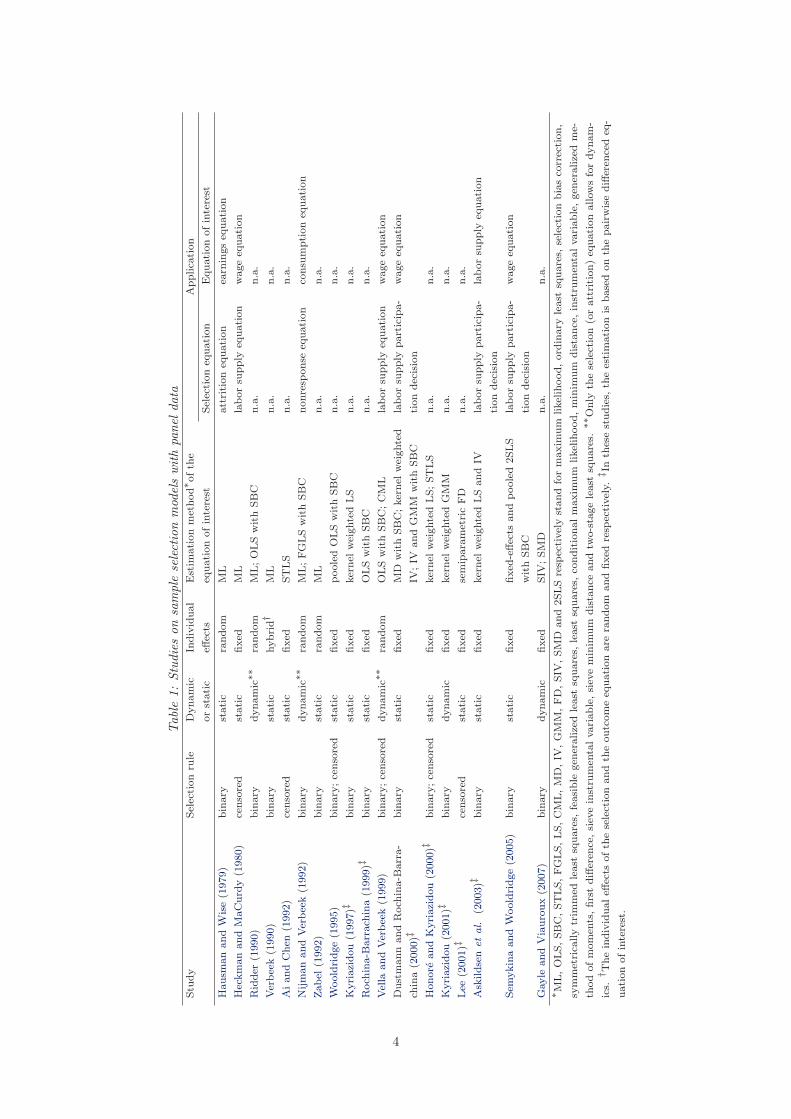
Most of the studies on panel data sample selection models are of the type 2 or type 3 tobit (see

Table 1), which are estimated by ML or two-step least squares (Heckman, 1979), or by variants of

the two-step Heckman type estimator.

For instance, Hausman and Wise (1979) describe a two-period model of attrition and estimate

by ML the impact of attrition on earnings. Attrition is defined as the inability to observe the

dependent variable of the equation of interest in the second period.5 Ridder (1990) generalizes

the model of Hausman and Wise to allow for more than two periods and attrition to occur also

in the first period. Hence Ridder’s model can be used as a standard attrition or sample selection

model. Nijman and Verbeek (1992) apply this model to study the effect of nonresponse on Dutch

households’ consumption. Verbeek (1990) assumes random and fixed individual effects in the

selection and regression equations respectively, and estimates by ML a transformed model with

a selection equation written in levels and a within-transformed equation of interest. Verbeek’s4The use of Gauss-Hermite quadrature, instead of simulated likelihood, is motivated by the finding of Guilkey

and Murphy (1993) that, for the same accuracy, the former method is 5 times as fast as the latter (see also Greene,2004b).

5Attrition in the first period is usually referred to as sample selection.

2

model is criticized by Zabel (1992) who considers random individual effects correlated with the

explanatory variables in both the selection equation and the equation of interest and estimates the

resulting model by ML. All these studies are of limited use to the applied researcher who wants to

implement the ML estimator as they present only the general expression of the likelihood function

which involves a multiple integral that is yet to be calculated. Our study makes a step in this

direction.

The two-step Heckman type estimator consists, in a first step, in estimating the selection

equation and constructing an estimate of a selection correction term that is included as a regressor

in the equation of interest which, in a second step, is estimated using ordinary least squares (OLS)

regression. Wooldridge (1995) estimates an augmented equation of interest written in levels by

pooled OLS where estimates of the selection correction terms are obtained, in a first step, using

a probit model for each period. Kyriazidou (1997) and Honore and Kyriazidou (2000) propose to

estimate, by kernel-weighted least squares, a pairwise differenced equation of interest for individuals

that are selected into the sample and have “the same” selection equation index in two different

periods. Under a conditional exchangeability assumption, the sample selection is time-invariant

for such individuals so that differencing the equation of interest over time wipes out, not only the

individual effects, but also the sample selection effect. In order to construct the kernel weights,

the parameters of the selection equation are estimated, in a first step, using conditional logit

or smoothed conditional maximum score. Rochina-Barrachina (1999) applies OLS to a pairwise

differenced equation of interest augmented with two selection correction terms for individuals that

are selected into the sample in two different periods. Estimates of these selection correction terms

are obtained, in a first step, using a bivariate probit for each combination of time periods. The

studies cited so far consider sample selection models with a binary selection rule (type 2 tobit).

Heckman and MaCurdy (1980) estimate by ML a fixed-effects type 3 tobit and apply it to

a wage equation with a labor supply (the number of hours worked) equation as the selection

equation. Ai and Chen (1992) and Honore and Kyriazidou (2000) estimate the same model using

symmetrically trimmed least squares (STLS), and Wooldridge (1995) uses the same estimator as

in his type 2 tobit case where estimates of the selection correction terms are now obtained, in a

first step, using a tobit model for each period. A Monte Carlo study comparing the estimators of

Wooldridge (1995), Honore and Kyriazidou (2000) and a semiparametric first-difference estimator

is provided by Lee (2001).

The above-mentioned studies on panel data sample selection models all assume strict exogene-

ity of the explanatory variables in the equation of interest. Models with censored endogenous

explanatory variables are studied by Vella and Verbeek (1999) and Askildsen et al. (2003), while

3

Tab

le1:

Stud

ies

onsa

mpl

ese

lect

ion

mod

els

with

pane

lda

taStu

dy

Sel

ecti

on

rule

Dynam

icIn

div

idual

Est

imati

on

met

hod∗ o

fth

eA

pplica

tion

or

stati

ceff

ects

equati

on

ofin

tere

stSel

ecti

on

equati

on

Equati

on

ofin

tere

st

Hausm

an

and

Wis

e(1

979)

bin

ary

stati

cra

ndom

ML

att

riti

on

equati

on

earn

ings

equati

on

Hec

km

an

and

MaC

urd

y(1

980)

censo

red

stati

cfixed

ML

labor

supply

equati

on

wage

equati

on

Rid

der

(1990)

bin

ary

dynam

ic∗∗

random

ML;O

LS

wit

hSB

Cn.a

.n.a

.

Ver

bee

k(1

990)

bin

ary

stati

chybri

d†

ML

n.a

.n.a

.

Aiand

Chen

(1992)

censo

red

stati

cfixed

ST

LS

n.a

.n.a

.

Nijm

an

and

Ver

bee

k(1

992)

bin

ary

dynam

ic∗∗

random

ML;FG

LS

wit

hSB

Cnonre

sponse

equati

on

consu

mpti

on

equati

on

Zabel

(1992)

bin

ary

stati

cra

ndom

ML

n.a

.n.a

.

Woold

ridge

(1995)

bin

ary

;ce

nso

red

stati

cfixed

poole

dO

LS

wit

hSB

Cn.a

.n.a

.

Kyri

azi

dou

(1997)‡

bin

ary

stati

cfixed

ker

nel

wei

ghte

dLS

n.a

.n.a

.

Roch

ina-B

arr

ach

ina

(1999)‡

bin

ary

stati

cfixed

OLS

wit

hSB

Cn.a

.n.a

.

Vel

laand

Ver

bee

k(1

999)

bin

ary

;ce

nso

red

dynam

ic∗∗

random

OLS

wit

hSB

C;C

ML

labor

supply

equati

on

wage

equati

on

Dust

mann

and

Roch

ina-B

arr

a-

bin

ary

stati

cfixed

MD

wit

hSB

C;ker

nel

wei

ghte

dla

bor

supply

part

icip

a-

wage

equati

on

chin

a(2

000)‡

IV;IV

and

GM

Mw

ith

SB

Cti

on

dec

isio

n

Honore

and

Kyri

azi

dou

(2000)‡

bin

ary

;ce

nso

red

stati

cfixed

ker

nel

wei

ghte

dLS;ST

LS

n.a

.n.a

.

Kyri

azi

dou

(2001)‡

bin

ary

dynam

icfixed

ker

nel

wei

ghte

dG

MM

n.a

.n.a

.

Lee

(2001)‡

censo

red

stati

cfixed

sem

ipara

met

ric

FD

n.a

.n.a

.

Ask

ildse

net

al.

(2003)‡

bin

ary

stati

cfixed

ker

nel

wei

ghte

dLS

and

IVla

bor

supply

part

icip

a-

labor

supply

equati

on

tion

dec

isio

n

Sem

ykin

aand

Woold

ridge

(2005)

bin

ary

stati

cfixed

fixed

-effec

tsand

poole

d2SLS

labor

supply

part

icip

a-

wage

equati

on

wit

hSB

Cti

on

dec

isio

n

Gayle

and

Via

uro

ux

(2007)

bin

ary

dynam

icfixed

SIV

;SM

Dn.a

.n.a

.∗ M

L,O

LS,SB

C,ST

LS,FG

LS,LS,C

ML,M

D,IV

,G

MM

,FD

,SIV

,SM

Dand

2SLS

resp

ecti

vel

yst

and

for

maxim

um

likel

ihood,ord

inary

least

square

s,se

lect

ion

bia

sco

rrec

tion,

sym

met

rica

lly

trim

med

least

square

s,fe

asi

ble

gen

eralize

dle

ast

square

s,le

ast

square

s,co

ndit

ionalm

axim

um

likel

ihood,m

inim

um

dis

tance

,in

stru

men

talvari

able

,gen

eralize

dm

e-

thod

ofm

om

ents

,firs

tdiff

eren

ce,si

eve

inst

rum

enta

lvari

able

,si

eve

min

imum

dis

tance

and

two-s

tage

least

square

s.∗∗

Only

the

sele

ctio

n(o

ratt

riti

on)

equati

on

allow

sfo

rdynam

-

ics.† T

he

indiv

idualeff

ects

ofth

ese

lect

ion

and

the

outc

om

eeq

uati

on

are

random

and

fixed

resp

ecti

vel

y.‡ I

nth

ese

studie

s,th

ees

tim

ati

on

isbase

don

the

pair

wis

ediff

eren

ced

eq-

uati

on

ofin

tere

st.

4

Dustmann and Rochina-Barrachina (2000) and Semykina and Wooldridge (2005) study models

with continuous endogenous explanatory variables. Vella and Verbeek (1999) estimate by OLS

with selection bias correction (SBC) a wage equation where labor supply enters the set of explana-

tory variables, and where estimates of the selection correction terms are obtained, in a first step,

using a dynamic tobit model of labor supply. Askildsen et al. (2003) estimate the wage elasticity

of labor supply for Norwegian nurses using an instrumental variable (IV) version of the Kyriazidou

(1997) method. Dustmann and Rochina-Barrachina (2000) and Semykina and Wooldridge (2005)

estimate the effect of experience, which is assumed to be endogenous, on wages. The former study

extends the Wooldridge (1995), Kyriazidou (1997) and Rochina-Barrachina (1999) estimators in

order to account for endogeneity in the explanatory variables, while the latter uses a pooled and

a fixed-effects two-stage least squares estimator with SBC. Finally, sample selection models that

allow for dynamics in both the selection equation and the equation of interest are studied by Kyri-

azidou (2001) who uses a two-step kernel weighted general method of moments (GMM) estimator,

and Gayle and Viauroux (2007) who use a sieve instrumental variable (SIV) and a sieve minimum

distance (SMD) estimator.

As Table 1 clearly shows, sample selection models with panel data are hardly studied in a

“full” dynamic framework where both the selection equation and the equation of interest include

a lagged dependent variable. Two exceptions are Kyriazidou (2001) and Gayle and Viauroux

(2007) who use semiparametric estimators for a fixed-effects dynamic panel data type 2 tobit.

This paper takes another route using ML to estimate a random-effects dynamic panel data type

2 tobit. Furthermore, while the literature considers only a static or “partial” dynamic panel data

type 3 tobit, we consider the estimation by ML of the model in a “full” dynamic framework.

An application of the model to study the dynamics of innovation in Dutch manufacturing is also

provided for the first time.

3 The model

The dynamic panel data sample selection model studied in this paper consists of two latent de-

pendent variables d∗it and y∗it written as

d∗it = ρdi,t−1 + δ′wit + ηi + ε1it, (1)

y∗it = γyi,t−1 + β′xit + αi + ε2it, (2)

5

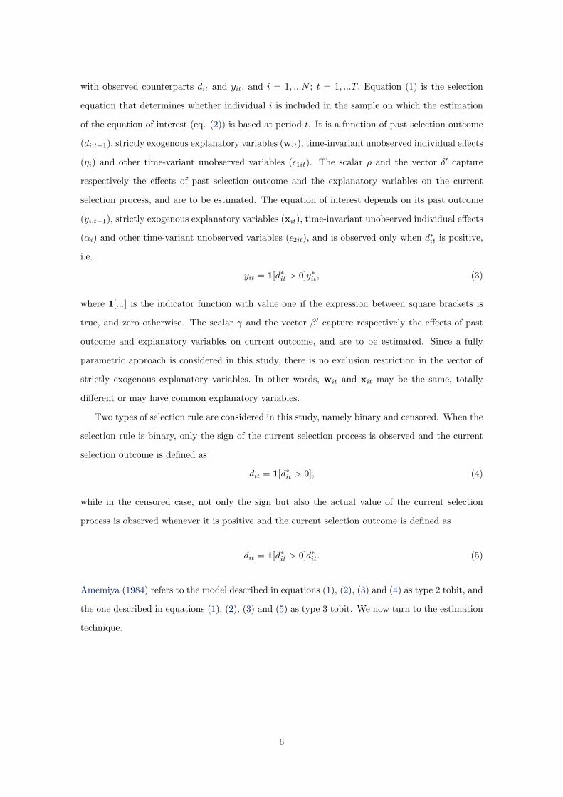
with observed counterparts dit and yit, and i = 1, ...N ; t = 1, ...T. Equation (1) is the selection

equation that determines whether individual i is included in the sample on which the estimation

of the equation of interest (eq. (2)) is based at period t. It is a function of past selection outcome

(di,t−1), strictly exogenous explanatory variables (wit), time-invariant unobserved individual effects

(ηi) and other time-variant unobserved variables (ε1it). The scalar ρ and the vector δ′ capture

respectively the effects of past selection outcome and the explanatory variables on the current

selection process, and are to be estimated. The equation of interest depends on its past outcome

(yi,t−1), strictly exogenous explanatory variables (xit), time-invariant unobserved individual effects

(αi) and other time-variant unobserved variables (ε2it), and is observed only when d∗it is positive,

i.e.

yit = 1[d∗it > 0]y∗it, (3)

where 1[...] is the indicator function with value one if the expression between square brackets is

true, and zero otherwise. The scalar γ and the vector β′ capture respectively the effects of past

outcome and explanatory variables on current outcome, and are to be estimated. Since a fully

parametric approach is considered in this study, there is no exclusion restriction in the vector of

strictly exogenous explanatory variables. In other words, wit and xit may be the same, totally

different or may have common explanatory variables.

Two types of selection rule are considered in this study, namely binary and censored. When the

selection rule is binary, only the sign of the current selection process is observed and the current

selection outcome is defined as

dit = 1[d∗it > 0], (4)

while in the censored case, not only the sign but also the actual value of the current selection

process is observed whenever it is positive and the current selection outcome is defined as

dit = 1[d∗it > 0]d∗it. (5)

Amemiya (1984) refers to the model described in equations (1), (2), (3) and (4) as type 2 tobit, and

the one described in equations (1), (2), (3) and (5) as type 3 tobit. We now turn to the estimation

technique.

6

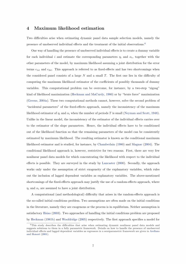
4 Maximum likelihood estimation

Two difficulties arise when estimating dynamic panel data sample selection models, namely the

presence of unobserved individual effects and the treatment of the initial observations.6

One way of handling the presence of unobserved individual effects is to create a dummy variable

for each individual i and estimate the corresponding parameters ηi and αi, together with the

other parameters of the model, by maximum likelihood assuming a joint distribution for the error

terms ε1it and ε2it. This approach is referred to as fixed-effects and has two shortcomings when

the considered panel consists of a large N and a small T . The first one lies in the difficulty of

computing the maximum likelihood estimator of the coefficients of possibly thousands of dummy

variables. This computational problem can be overcome, for instance, by a two-step “zigzag”

kind of likelihood maximization (Heckman and MaCurdy, 1980) or by “brute force” maximization

(Greene, 2004a). These two computational methods cannot, however, solve the second problem of

“incidental parameters” of the fixed-effects approach, namely the inconsistency of the maximum

likelihood estimator of ηi and αi when the number of periods T is small (Neyman and Scott, 1948).

Unlike in the linear model, the inconsistency of the estimator of the individual effects carries over

to the estimator of the slope parameters. Hence, the individual effects have to be conditioned

out of the likelihood function so that the remaining parameters of the model can be consistently

estimated by maximum likelihood. The resulting estimator is known as the conditional maximum

likelihood estimator and is studied, for instance, by Chamberlain (1980) and Magnac (2004). The

conditional likelihood approach is, however, restrictive for two reasons. First, there are very few

nonlinear panel data models for which concentrating the likelihood with respect to the individual

effects is possible. They are surveyed in the study by Lancaster (2000). Secondly, the approach

works only under the assumption of strict exogeneity of the explanatory variables, which rules

out the inclusion of lagged dependent variables as explanatory variables. The above-mentioned

shortcomings of the fixed-effects approach may justify the use of a random-effects approach, where

ηi and αi are assumed to have a joint distribution.

A computational (and methodological) difficulty that arises in the random-effects approach is

the so-called initial conditions problem. Two assumptions are often made on the initial conditions

in the literature, namely they are exogenous or the process is in equilibrium. Neither assumption is

satisfactory Hsiao (2003). Two approaches of handling the initial conditions problem are proposed

by Heckman (1981b) and Wooldridge (2005) respectively. The first approach specifies a model for

6This study describes the difficulties that arise when estimating dynamic nonlinear panel data models andsuggests solutions to them in a fully parametric framework. Details on how to handle the presence of unobservedindividual effects and lagged dependent variables as regressors in a semiparametric framework are given in Arellanoand Honore (2001).

7

the initial conditions given the individual effects and the strictly exogenous explanatory variables.

In empirical work, this model is often assumed to be similar to the model underlying the remain-

ing process. For instance, if the underlying model is a dynamic panel data probit, the model at

the initial period is assumed to be standard probit. A likelihood function which is marginal to

both the individual effects and the initial conditions can be derived and maximized using standard

numerical procedures. The second approach specifies a distribution for the individual effects con-

ditional on the initial conditions and the strictly exogenous explanatory variables. In this case, the

likelihood function is marginal to the individual effects but conditional on the initial conditions.

Both approaches are legitimate and yield consistent estimates of the parameters of the model under

the assumption of correct specification of the distribution of the errors. However, the Wooldridge

approach is easier to implement, which has made it more popular in applied econometrics recently,

and more flexible in the sense that it applies to a wide range of nonlinear dynamic panel data

models and allows, unlike the Heckman approach, for individual effects to be correlated with the

strictly exogenous explanatory variables (see Raymond, 2007). The likelihood function derived in

the Wooldridge approach has the same structure for both the dynamic and the static versions of

the nonlinear model. This study extends this approach to models that contain more than one

equation. The approach is described as follows.

The individual effects are assumed, in each period, to be linear in the strictly exogenous ex-

planatory variables and the initial conditions, i.e.

ηi = bs0 + bs

1di0 + b′s2 wi + a1i, (6)

αi = br0 + br

1yi0 + b′r2 xi + a2i, (7)

where w′i = (w′

i1, ...,w′iT ), x′i = (x′i1, ...,x

′iT ), bs

0, bs1, b

′s2 , br

0, br1 and b′r2 are to be estimated, and a1i

and a2i are independent of (di0,wi) and (yi0,xi) respectively.7 The scalars bs1 and br

1 capture the

dependence of the individual effects on the initial conditions. The vectors (ε1it, ε2it)′ and (a1i, a2i)′

are assumed to be independent of each other, and independently and identically distributed over

time and across individuals following a normal distribution with mean zero and covariance matrices

Ωε1ε2 =

σ2ε1 ρε1ε2σε1σε2

ρε1ε2σε1σε2 σ2ε2

and Ωa1a2 =

σ2a1

ρa1a2σa1σa2

ρa1a2σa1σa2 σ2a2

(8)

respectively. The parameters of the covariance matrices are also to be estimated. Hence, the7The vectors of explanatory variables wi and xi, in order to be included in equations (6) and (7), must be

sufficiently time-variant, otherwise a collinearity problem will arise.

8

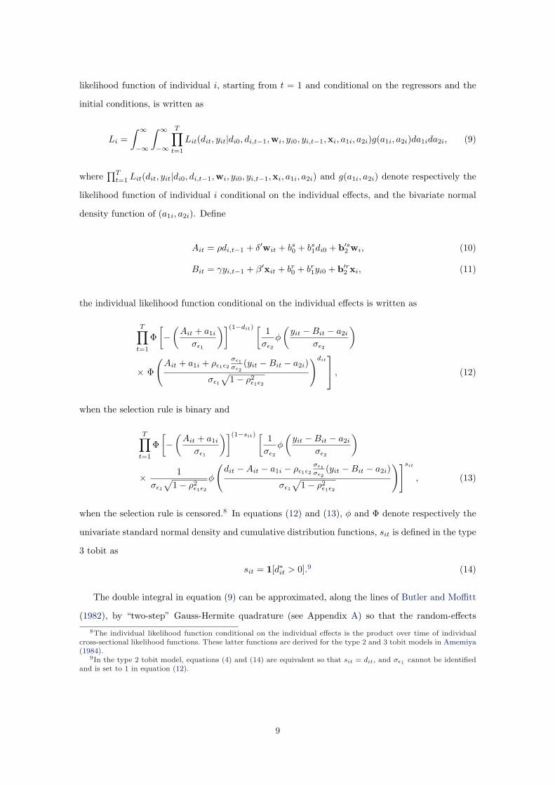
likelihood function of individual i, starting from t = 1 and conditional on the regressors and the

initial conditions, is written as

Li =∫ ∞

−∞

∫ ∞

−∞

T∏t=1

Lit(dit, yit|di0, di,t−1,wi, yi0, yi,t−1,xi, a1i, a2i)g(a1i, a2i)da1ida2i, (9)

where∏T

t=1 Lit(dit, yit|di0, di,t−1,wi, yi0, yi,t−1,xi, a1i, a2i) and g(a1i, a2i) denote respectively the

likelihood function of individual i conditional on the individual effects, and the bivariate normal

density function of (a1i, a2i). Define

Ait = ρdi,t−1 + δ′wit + bs0 + bs

1di0 + b′s2 wi, (10)

Bit = γyi,t−1 + β′xit + br0 + br

1yi0 + b′r2 xi, (11)

the individual likelihood function conditional on the individual effects is written as

T∏t=1

Φ[−

(Ait + a1i

σε1

)](1−dit) [1

σε2

φ

(yit −Bit − a2i

σε2

)

× Φ

(Ait + a1i + ρε1ε2

σε1σε2

(yit −Bit − a2i)

σε1

√1− ρ2

ε1ε2

)dit , (12)

when the selection rule is binary and

T∏t=1

Φ[−

(Ait + a1i

σε1

)](1−sit) [1

σε2

φ

(yit −Bit − a2i

σε2

)

× 1σε1

√1− ρ2

ε1ε2

φ

(dit −Ait − a1i − ρε1ε2

σε1σε2

(yit −Bit − a2i)

σε1

√1− ρ2

ε1ε2

)]sit

, (13)

when the selection rule is censored.8 In equations (12) and (13), φ and Φ denote respectively the

univariate standard normal density and cumulative distribution functions, sit is defined in the type

3 tobit as

sit = 1[d∗it > 0].9 (14)

The double integral in equation (9) can be approximated, along the lines of Butler and Moffitt

(1982), by “two-step” Gauss-Hermite quadrature (see Appendix A) so that the random-effects

8The individual likelihood function conditional on the individual effects is the product over time of individualcross-sectional likelihood functions. These latter functions are derived for the type 2 and 3 tobit models in Amemiya(1984).

9In the type 2 tobit model, equations (4) and (14) are equivalent so that sit = dit, and σε1 cannot be identifiedand is set to 1 in equation (12).

9

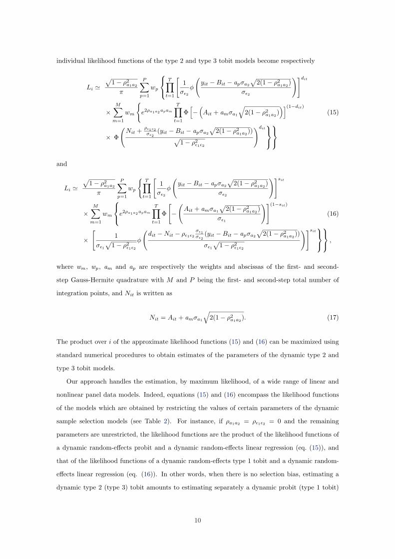
individual likelihood functions of the type 2 and type 3 tobit models become respectively

Li '√

1− ρ2a1a2

π

P∑p=1

wp

T∏t=1

[1

σε2

φ

(yit −Bit − apσa2

√2(1− ρ2

a1a2)

σε2

)]dit

×M∑

m=1

wm

e2ρa1a2apam

T∏t=1

Φ[−

(Ait + amσa1

√2(1− ρ2

a1a2))](1−dit)

(15)

× Φ

(Nit + ρε1ε2

σε2(yit −Bit − apσa2

√2(1− ρ2

a1a2))

√1− ρ2

ε1ε2

)dit

and

Li '√

1− ρ2a1a2

π

P∑p=1

wp

T∏

t=1

[1

σε2

φ

(yit −Bit − apσa2

√2(1− ρ2

a1a2)

σε2

)]sit

×M∑

m=1

wm

e2ρa1a2apam

T∏t=1

Φ

[−

(Ait + amσa1

√2(1− ρ2

a1a2)

σε1

)](1−sit)

(16)

×[

1σε1

√1− ρ2

ε1ε2

φ

(dit −Nit − ρε1ε2

σε1σε2

(yit −Bit − apσa2

√2(1− ρ2

a1a2))

σε1

√1− ρ2

ε1ε2

)]sit

,

where wm , wp , am and ap are respectively the weights and abscissas of the first- and second-

step Gauss-Hermite quadrature with M and P being the first- and second-step total number of

integration points, and Nit is written as

Nit = Ait + amσa1

√2(1− ρ2

a1a2). (17)

The product over i of the approximate likelihood functions (15) and (16) can be maximized using

standard numerical procedures to obtain estimates of the parameters of the dynamic type 2 and

type 3 tobit models.

Our approach handles the estimation, by maximum likelihood, of a wide range of linear and

nonlinear panel data models. Indeed, equations (15) and (16) encompass the likelihood functions

of the models which are obtained by restricting the values of certain parameters of the dynamic

sample selection models (see Table 2). For instance, if ρa1a2 = ρε1ε2 = 0 and the remaining

parameters are unrestricted, the likelihood functions are the product of the likelihood functions of

a dynamic random-effects probit and a dynamic random-effects linear regression (eq. (15)), and

that of the likelihood functions of a dynamic random-effects type 1 tobit and a dynamic random-

effects linear regression (eq. (16)). In other words, when there is no selection bias, estimating a

dynamic type 2 (type 3) tobit amounts to estimating separately a dynamic probit (type 1 tobit)

10

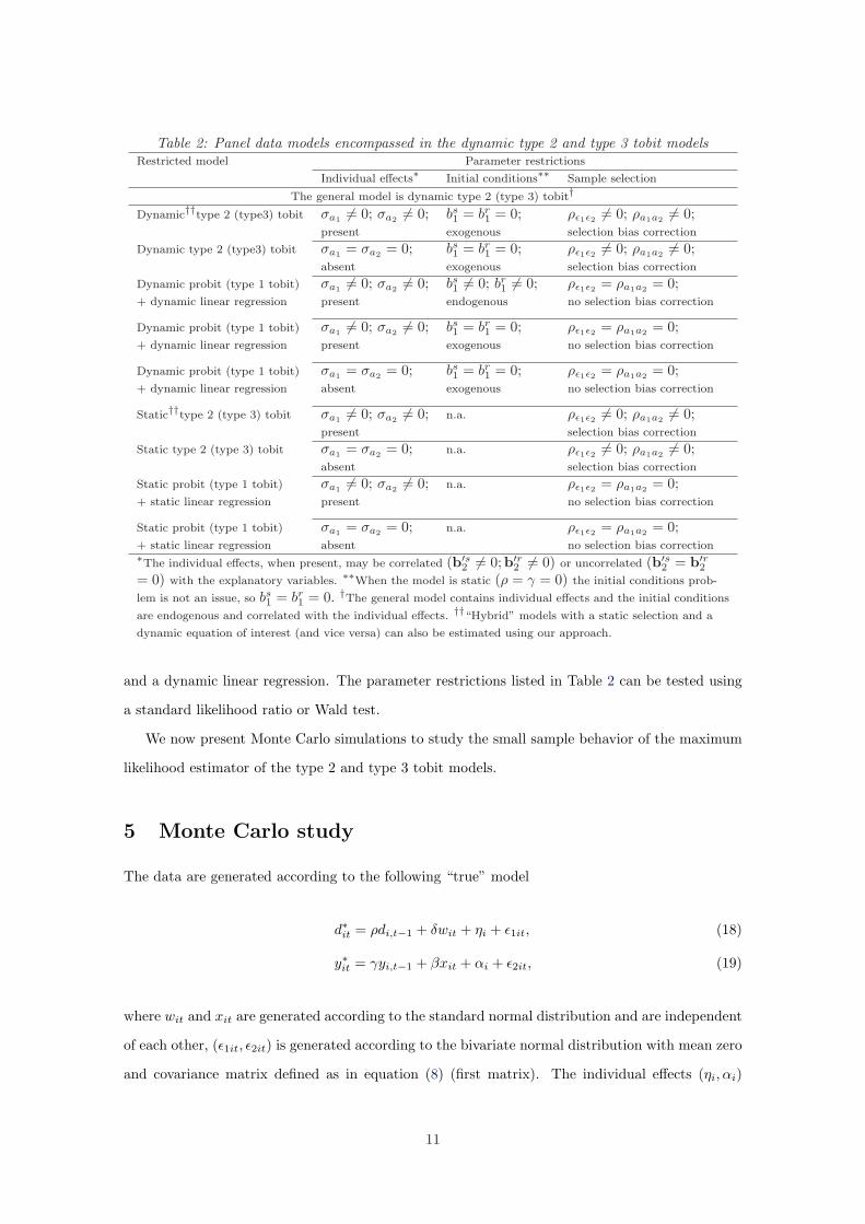
Table 2: Panel data models encompassed in the dynamic type 2 and type 3 tobit modelsRestricted model Parameter restrictions

Individual effects∗ Initial conditions∗∗ Sample selection

The general model is dynamic type 2 (type 3) tobit†

Dynamic††type 2 (type3) tobit σa1 6= 0; σa2 6= 0; bs1 = br

1 = 0; ρε1ε2 6= 0; ρa1a2 6= 0;present exogenous selection bias correction

Dynamic type 2 (type3) tobit σa1 = σa2 = 0; bs1 = br

1 = 0; ρε1ε2 6= 0; ρa1a2 6= 0;absent exogenous selection bias correction

Dynamic probit (type 1 tobit) σa1 6= 0; σa2 6= 0; bs1 6= 0; br

1 6= 0; ρε1ε2 = ρa1a2 = 0;+ dynamic linear regression present endogenous no selection bias correction

Dynamic probit (type 1 tobit) σa1 6= 0; σa2 6= 0; bs1 = br

1 = 0; ρε1ε2 = ρa1a2 = 0;+ dynamic linear regression present exogenous no selection bias correction

Dynamic probit (type 1 tobit) σa1 = σa2 = 0; bs1 = br

1 = 0; ρε1ε2 = ρa1a2 = 0;+ dynamic linear regression absent exogenous no selection bias correction

Static††type 2 (type 3) tobit σa1 6= 0; σa2 6= 0; n.a. ρε1ε2 6= 0; ρa1a2 6= 0;present selection bias correction

Static type 2 (type 3) tobit σa1 = σa2 = 0; n.a. ρε1ε2 6= 0; ρa1a2 6= 0;absent selection bias correction

Static probit (type 1 tobit) σa1 6= 0; σa2 6= 0; n.a. ρε1ε2 = ρa1a2 = 0;+ static linear regression present no selection bias correction

Static probit (type 1 tobit) σa1 = σa2 = 0; n.a. ρε1ε2 = ρa1a2 = 0;+ static linear regression absent no selection bias correction∗The individual effects, when present, may be correlated (b′s2 6= 0;b′r2 6= 0) or uncorrelated (b′s2 = b′r2= 0) with the explanatory variables. ∗∗When the model is static (ρ = γ = 0) the initial conditions prob-

lem is not an issue, so bs1 = br

1 = 0. †The general model contains individual effects and the initial conditions

are endogenous and correlated with the individual effects. ††“Hybrid” models with a static selection and a

dynamic equation of interest (and vice versa) can also be estimated using our approach.

and a dynamic linear regression. The parameter restrictions listed in Table 2 can be tested using

a standard likelihood ratio or Wald test.

We now present Monte Carlo simulations to study the small sample behavior of the maximum

likelihood estimator of the type 2 and type 3 tobit models.

5 Monte Carlo study

The data are generated according to the following “true” model

d∗it = ρdi,t−1 + δwit + ηi + ε1it, (18)

y∗it = γyi,t−1 + βxit + αi + ε2it, (19)

where wit and xit are generated according to the standard normal distribution and are independent

of each other, (ε1it, ε2it) is generated according to the bivariate normal distribution with mean zero

and covariance matrix defined as in equation (8) (first matrix). The individual effects (ηi, αi)

11

are generated independently of (ε1it, ε2it) according to the bivariate normal distribution with mean

(di0, yi0) and covariance matrix defined as in equation (8) (second matrix). The dependent variables

of the equation of interest and the selection rules are defined as in equations (3-5), i.e., both the type

2 and type 3 tobit are considered. The true parameter values are δ = β = 1, σa1 = σa2 = σε2 = 0.5,

σε1 = 1, ρa1a2 = 0.5, ρε1ε2 = 0.8, and two sets of values are chosen for ρ and γ, namely ρ = γ = 0

when the model is static, and ρ = γ = 0.5 when the model is dynamic. All dynamic and static

data generating processes considered include individual effects.

Given these values of the parameters, sample selection is not constant over time, i.e. the

selection outcome dit (or sit) has a rather high within standard deviation (around 0.40) for the

(dynamic and static) type 2 and type 3 tobit. Furthermore, the censoring rate over the whole

period, for both models, is approximately 40% and 50% in the dynamic and the static settings

respectively. Finally, the correlation between the individual effects and the initial conditions for

the type 2 and type 3 tobit is 0.70 and 0.80 in the selection equation, and 0.80 for both models in

the equation of interest.

To summarize, the data generating process (DGP) at the initial period is standard type 2

(type 3) tobit while the remaining period DGP is dynamic type 2 (type 3) tobit with endogenous

initial conditions correlated with the individual effects, and accounting for selection bias correction

(SBC). The static DGP is obtained by setting the true values of ρ, γ to 0.

The estimation results of ρ, γ, δ, β, σa1 , σa2 , ρa1a2 and ρε1ε2 based on 200 replications are shown

in Tables 3-8 for the following sample sizes: N = 500 and T = 4, N = 500 and T = 7, and N = 800

and T = 4. We report the mean and standard deviation over the replications of these estimates.10

In each replication, the estimation is based on T − 1 periods, the first one being the initial period.

We study the small sample behavior of the maximum likelihood estimator (MLE) of the above-

mentioned parameters when the model is both correctly and incorrectly specified. More specifically,

when the DGP is dynamic, misspecification includes a dynamic model with no individual effects

but SBC; with individual effects, exogenous initial conditions and SBC; with individual effects,

endogenous initial conditions but no SBC; and a static model with individual effects and SBC.

When the DGP is static, misspecification includes a static model with no individual effects but

SBC; with individual effects but no SBC; and a dynamic model with no individual effects but SBC,

and with individual effects and endogenous initial conditions correlated with the individual effects

and SBC.

We now discuss the Monte Carlo results.10We do not report the estimate results of σε1 (for the type 3 tobit), σε2 , and the additional parameters of

equations (6) and (7).

12

5.1 The MLE behavior when the model is correctly specified

The mean and standard deviation of the MLE of ρ, γ, δ, β, σa1 , σa2 , ρa1a2 and ρε1ε2 , when the

model is correctly specified, are reported in Table 3.

The MLE of δ and β in both the dynamic and static type 2 and type 3 tobit is biased towards

zero. The bias does not exceed 2% and 0.7% for δ and β in the type 2 tobit, and 3.5% and 0.8%

in the type 3 tobit. There is no clear pattern of bias reduction as either T or N increases. In all

cases but the dynamic type 2 tobit with N = 800 and T = 4, the estimate of β is on average closer

to the true value than that of δ. In both the type 2 and type 3 tobit, the estimates of δ and β are

closer to the true values in the static case than in the dynamic case, except in the dynamic type

2 tobit with N = 800 and T = 4 where the pattern shows up the other way round in the estimate

of δ. From this, we can conclude that it is more difficult to estimate accurately the coefficients

of the strictly exogenous explanatory variables in both the selection equation and the equation of

interest of dynamic panel data sample selection models than those of their static counterparts.

The MLE of ρ and γ is also biased towards zero in both the dynamic type 2 and type 3 tobit.

The bias does not exceed 2% and 4.7% for ρ and γ in the type 2 tobit, and 3.5% and 4.2% in the

type 3 tobit. Like δ and β, there is no clear pattern of bias reduction as either T or N increases,

and the MLE bias of ρ and γ is overall larger than that of δ and β. As a result, we can state that

it is more difficult to estimate accurately the coefficients of the lagged dependent variables than

those of the strictly exogenous variables in both the selection equation and the equation of interest

of dynamic panel data sample selection models.

In both models, σa1 and σa2 are much less accurately estimated than ρ, γ, δ and β, even though

their bias remains towards zero. For both models, the bias is smaller in the static case than in the

dynamic case. In all cases but, for σa1 when N = 500 and T = 7, the bias is smaller in the type 2

tobit than in the type 3 tobit. The two models exhibit different patterns in the bias reduction as T

increases. Indeed, the type 2 tobit shows an increase in the MLE bias of σa1 and σa2 which is more

pronounced for σa1 than it is for σa2 . The increase in the MLE bias of σa1 , as T increases, confirms

the results by Rabe-Hesketh et al. (2005) that show that the MLE of the standard deviation of

the individual effects in random-effects probit models is biased away from zero for large cluster

size T , with a bias that ranges from 19% for T as small as 10 to 178% for T as large as 500. The

type 3 tobit on the other hand shows a decrease in the bias of the MLE of σa1 and σa2 which is

more pronounced for σa1 than it is for σa2 . As N increases, the bias reduction pattern is not clear

cut, especially in the type 3 tobit.

Finally, in both models, the MLE of ρa1a2 is biased away from zero with a bias of about 25%,

13

Tab

le3:

ML

estim

ates

base

don

200

repl

icat

ions

and

2-po

intG

auss

-Her

mite

quad

ratu

re:

Dat

age

nera

ting

proc

ess

(Tru

evalu

e)∗

Est

imate

Mea

nStd

.D

ev.

Mea

nStd

.D

ev.

Mea

nStd

.D

ev.

Mea

nStd

.D

ev.

Est

imate

dm

odel

Sta

tic

type

2to

bit

Dynam

icty

pe

2to

bit

Sta

tic

type

3to

bit

Dynam

icty

pe

3to

bit

N=

500;T

=4

(ρ=

0.5)

ρ-

-0.4

80

(0.0

86)

--

0.4

74

(0.0

23)

(γ=

0.5)

γ-

-0.5

41

(0.0

18)

--

0.5

40

(0.0

16)

(δ=

1.0)

δ0.9

91

(0.0

50)

1.0

16

(0.0

55)

0.9

97

(0.0

27)

1.0

24

(0.0

25)

(β=

1.0)

β1.0

01

(0.0

21)

1.0

07

(0.0

19)

1.0

02

(0.0

18)

1.0

08

(0.0

16)

(σa1

=0.

5)σ

a1

0.5

21

(0.0

77)

0.5

57

(0.0

96)

0.4

34

(0.0

70)

0.4

12

(0.0

75)

(σa2

=0.

5)σ

a2

0.4

48

(0.0

21)

0.4

09

(0.0

58)

0.4

21

(0.0

18)

0.3

71

(0.1

08)

(ρa1a2

=0.

5)ρ

a1a2

0.2

78

(0.0

14)

0.2

83

(0.0

41)

0.2

56

(0.0

17)

0.2

36

(0.0

70)

(ρε 1

ε 2=

0.8)

ρε 1

ε 20.6

82

(0.0

47)

0.6

03

(0.0

72)

0.7

09

(0.0

24)

0.7

40

(0.0

22)

N=

500;T

=7

(ρ=

0.5)

ρ-

-0.4

89

(0.0

58)

--

0.4

65

(0.0

15)

(γ=

0.5)

γ-

-0.5

45

(0.0

12)

--

0.5

39

(0.0

11)

(δ=

1.0)

δ0.9

99

(0.0

41)

1.0

20

(0.0

43)

0.9

98

(0.0

21)

1.0

35

(0.0

18)

(β=

1.0)

β1.0

00

(0.0

14)

1.0

05

(0.0

13)

1.0

00

(0.0

11)

1.0

05

(0.0

09)

(σa1

=0.

5)σ

a1

0.5

81

(0.0

53)

0.5

93

(0.0

65)

0.5

26

(0.0

52)

0.5

32

(0.0

54)

(σa2

=0.

5)σ

a2

0.4

46

(0.0

14)

0.3

97

(0.0

58)

0.4

29

(0.0

13)

0.3

91

(0.0

14)

(ρa1a2

=0.

5)ρ

a1a2

0.3

08

(0.0

14)

0.3

08

(0.0

45)

0.2

76

(0.0

16)

0.2

56

(0.0

21)

(ρε 1

ε 2=

0.8)

ρε 1

ε 20.6

85

(0.0

38)

0.6

18

(0.0

54)

0.7

14

(0.0

17)

0.7

50

(0.0

13)

N=

800;T

=4

(ρ=

0.5)

ρ-

-0.4

80

(0.0

62)

--

0.4

77

(0.0

16)

(γ=

0.5)

γ-

-0.5

41

(0.0

15)

--

0.5

42

(0.0

13)

(δ=

1.0)

δ0.9

86

(0.0

38)

1.0

05

(0.0

42)

0.9

93

(0.0

21)

1.0

20

(0.0

19)

(β=

1.0)

β1.0

00

(0.0

17)

1.0

06

(0.0

14)

0.9

99

(0.0

14)

1.0

08

(0.0

12)

(σa1

=0.

5)σ

a1

0.5

16

(0.0

64)

0.5

42

(0.0

68)

0.4

37

(0.0

54)

0.4

07

(0.0

59)

(σa2

=0.

5)σ

a2

0.4

47

(0.0

17)

0.4

09

(0.0

57)

0.4

19

(0.0

14)

0.3

87

(0.0

14)

(ρa1a2

=0.

5)ρ

a1a2

0.2

80

(0.0

10)

0.2

87

(0.0

41)

0.2

56

(0.0

11)

0.2

48

(0.0

13)

(ρε 1

ε 2=

0.8)

ρε 1

ε 20.6

80

(0.0

35)

0.6

04

(0.0

53)

0.7

07

(0.0

19)

0.7

40

(0.0

17)

∗ ρ=

γ=

0in

the

stati

cdata

gen

erati

ng

pro

cess

.

14

while that of ρε1ε2 is biased away from zero in the type 2 tobit and towards zero in the type 3

tobit. This bias decreases only slightly as T increases, while there is no clear pattern of reduction

as N increases.

To summarize, we can state that, when the model is correctly specified, the MLE bias of

the parameters of panel data sample selection models is very small for a sample size as large as

the one considered in the Monte Carlo study. The “two-step” Gauss-Hermite quadrature used

to approximate the likelihood function works very well, even for a number of integration points,

in each step, as small as 2. However, the standard deviations of the individual effects and the

sample selection terms are less accurately estimated than the remaining parameters of Table 3.

Accuracy in the estimates can be gained by either increasing the number of integration points or

using adaptive Gauss-Hermite quadrature in the spirit of Rabe-Hesketh et al. (2005).11

We now discuss the behavior of the MLE when the model is incorrectly specified.

5.2 The MLE behavior when the model is incorrectly specified

The mean and standard deviation of the MLE of ρ, γ, δ, β, σa1 , σa2 , ρa1a2 and ρε1ε2 , when the

model is incorrectly specified, are reported in Tables 4-8. More specifically, we study the finite

sample bias of the MLE when we fail to account for individual effects, when we assume exogenous

initial conditions and when we fail to correct for selection bias. We also study the case where a

static model is estimated under a dynamic DGP and vice versa. All DGPs considered include

individual effects.

5.2.1 No individual effects

Table 4 reports the mean and standard deviation of the MLE of ρ, γ, δ, β and ρε1ε2 when the

individual effects, while being present in the DGP, are ignored in the estimation of the model, i.e.,

σa1 , σa2 and ρa1a2 are all assumed to be zero.

The MLE of β remains biased towards zero in all cases. In other words, the MLE bias of the

coefficient of the strictly exogenous explanatory variable in the equation of interest is unaffected

if we fail to account for individual effects. This result holds regardless of the type of the selection

rule, and regardless of whether the model is dynamic or static. The MLE of δ also remains biased

towards zero in the type 3 tobit and in the static type 2 tobit with a larger bias than that of β.

In the dynamic type 2 tobit, however, the MLE of δ is biased away from zero with a bias that is11In the study by Rabe-Hesketh et al. (2005), adaptive Gauss-Hermite quadrature is shown to work better than

normal Gauss-Hermite quadrature in static random-effects probit models when T or the equicorrelation is verylarge. The use of adaptive Gauss-Hermite quadrature can be generalized to sample selection models but is beyondthe scope of this study.

15

Tab

le4:

ML

estim

ates

base

don

200

repl

icat

ions

and

2-po

intG

auss

-Her

mite

quad

ratu

re:

No

indi

vidu

aleff

ects

(Tru

evalu

e)∗

Est

imate

Mea

nStd

.D

ev.

Mea

nStd

.D

ev.

Mea

nStd

.D

ev.

Mea

nStd

.D

ev.

Est

imate

dm

odel

Sta

tic

type

2to

bit

Dynam

icty

pe

2to

bit

Sta

tic

type

3to

bit

Dynam

icty

pe

3to

bit

N=

500;T

=4

(ρ=

0.5)

ρ-

-1.1

06

(0.0

61)

--

0.9

89

(0.0

19)

(γ=

0.5)

γ-

-1.0

46

(0.0

20)

--

1.0

47

(0.0

19)

(δ=

1.0)

δ0.9

01

(0.0

42)

0.8

41

(0.0

45)

1.0

02

(0.0

26)

1.0

49

(0.0

36)

(β=

1.0)

β1.0

02

(0.0

23)

1.0

02

(0.0

31)

1.0

01

(0.0

20)

1.0

02

(0.0

26)

(ρε 1

ε 2=

0.8)

ρε 1

ε 20.6

64

(0.0

31)

0.4

73

(0.0

65)

0.6

66

(0.0

21)

0.5

35

(0.0

28)

N=

500;T

=7

(ρ=

0.5)

ρ-

-1.0

36

(0.0

40)

--

0.9

07

(0.0

15)

(γ=

0.5)

γ-

-0.9

63

(0.0

12)

--

0.9

63

(0.0

14)

(δ=

1.0)

δ0.9

00

(0.0

34)

0.8

28

(0.0

35)

1.0

02

(0.0

21)

1.0

57

(0.0

25)

(β=

1.0)

β1.0

00

(0.0

17)

1.0

00

(0.0

18)

1.0

01

(0.0

14)

1.0

02

(0.0

18)

(ρε 1

ε 2=

0.8)

ρε 1

ε 20.6

65

(0.0

25)

0.4

28

(0.0

52)

0.6

63

(0.0

17)

0.5

34

(0.0

23)

N=

800;T

=4

(ρ=

0.5)

ρ-

-1.1

03

(0.0

43)

--

0.9

89

(0.0

14)

(γ=

0.5)

γ-

-1.0

46

(0.0

15)

--

1.0

48

(0.0

16)

(δ=

1.0)

δ0.8

96

(0.0

33)

0.8

32

(0.0

36)

0.9

97

(0.0

21)

1.0

48

(0.0

29)

(β=

1.0)

β1.0

01

(0.0

18)

1.0

00

(0.0

21)

0.9

99

(0.0

14)

1.0

02

(0.0

21)

(ρε 1

ε 2=

0.8)

ρε 1

ε 20.6

64

(0.0

24)

0.4

73

(0.0

49)

0.6

64

(0.0

18)

0.5

31

(0.0

22)

∗ ρ=

γ=

0in

the

stati

cdata

gen

erati

ng

pro

cess

.T

he

indiv

idualeff

ects

,w

hile

bei

ng

pre

sent

inth

edata

gen

erati

ng

pro

cess

,are

ignore

din

the

esti

mati

on

ofth

em

odel

.

16

always larger than 15%. Hence, unlike β, when we fail to account for individual effects, the MLE

behavior of the coefficient of the strictly exogenous explanatory variable in the selection equation

differs according to the type of the selection rule and according to whether the model is dynamic

or static.

In the dynamic version of the model, the MLE of ρ and γ is biased away from zero and upwards

in all cases, with a bias that gets as large as 61% in the type 2 tobit, and 55% in the type 3 tobit.

This bias is reduced fairly substantially (by about 9%) as T increases but remains very high, and

is unchanged as N increases. In other words, when estimating the dynamic version of the model

and failing to account for individual effects, the coefficients of the lagged dependent explanatory

variables, in both the selection equation and the equation of interest, are overestimated. In the

dynamic panel data discrete choice model, this phenomenon is known as spurious state dependence

(Heckman, 1981a), i.e. too much credit is attributed to past event as a determinant of current

event if intertemporal correlation in the unobservables is not accounted for.

Finally, the MLE of ρε1ε2 is biased away from zero with a bias of about 25% in the static case,

and about 35% in the dynamic case. There is no clear pattern of bias reduction as either T or N

increases.

5.2.2 Exogenous initial conditions

Table 5 reports the mean and standard deviation of the MLE of ρ, γ, δ, β, σa1 , σa2 , ρa1a2 and ρε1ε2

when the initial conditions, while being endogenous and correlated with the individual effects in

the DGP, are assumed to be exogenous, i.e., bs1 and br

1 are assumed to be zero.

In both the type 2 and type 3 tobit, the MLE bias of δ and β increases by about 6% with

respect to the case of the DGP but remains fairly small, less than 9% in the type 2 tobit, and less

than 11% in the type 3 tobit. As for the MLE of ρ and γ, their bias remains substantially large

compared to the case where the individual effects are ignored. Accounting for individual effects

but assuming exogenous initial conditions also results in a spurious state dependence situation.12

Hence, we can state that, in order for the coefficients of the lagged dependent explanatory variables

to be accurately estimated, the correlation between the initial conditions and the individual effects

must be taken into account: controlling for individual effects only is not sufficient. As T increases,

the MLE bias of ρ and γ, in both the type 2 and type 3 tobit, decreases by about 10% but remains

substantially large, while, as N increases, the bias remains the same. Finally, the MLE bias of

ρa1a2 and ρε1ε2 is higher than in the DGP case, and that of σa1 and σa2 is comparable to that of

12Although the term spurious state dependence was used in the context of discrete choice models, we use it inour study to explain the overestimation of the coefficients of the lagged dependent explanatory variables in boththe selection equation and the equation of interest.

17

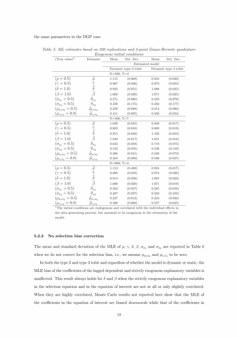
the same parameters in the DGP case.

Table 5: ML estimates based on 200 replications and 2-point Gauss-Hermite quadrature:Exogenous initial conditions

(True value)∗ Estimate Mean Std. Dev. Mean Std. Dev.

Estimated model

Dynamic type 2 tobit Dynamic type 3 tobit

N=500; T=4

(ρ = 0.5) ρ 1.115 (0.069) 0.924 (0.020)

(γ = 0.5) γ 0.967 (0.026) 0.973 (0.024)

(δ = 1.0) δ 0.923 (0.051) 1.086 (0.035)

(β = 1.0) β 1.062 (0.030) 1.071 (0.025)

(σa1 = 0.5) σa1 0.571 (0.080) 0.583 (0.078)

(σa2 = 0.5) σa2 0.458 (0.175) 0.482 (0.177)

(ρa1a2 = 0.5) ρa1a2 0.229 (0.088) 0.214 (0.080)

(ρε1ε2 = 0.8) ρε1ε2 0.411 (0.095) 0.560 (0.034)

N=500; T=7

(ρ = 0.5) ρ 1.030 (0.045) 0.829 (0.017)

(γ = 0.5) γ 0.863 (0.016) 0.869 (0.019)

(δ = 1.0) δ 0.915 (0.040) 1.102 (0.024)

(β = 1.0) β 1.048 (0.017) 1.051 (0.016)

(σa1 = 0.5) σa1 0.632 (0.058) 0.718 (0.075)

(σa2 = 0.5) σa2 0.532 (0.076) 0.538 (0.159)

(ρa1a2 = 0.5) ρa1a2 0.266 (0.041) 0.240 (0.073)

(ρε1ε2 = 0.8) ρε1ε2 0.403 (0.080) 0.586 (0.027)

N=800; T=4

(ρ = 0.5) ρ 1.113 (0.480) 0.924 (0.017)

(γ = 0.5) γ 0.968 (0.019) 0.974 (0.020)

(δ = 1.0) δ 0.914 (0.039) 1.085 (0.029)

(β = 1.0) β 1.060 (0.020) 1.071 (0.019)

(σa1 = 0.5) σa1 0.563 (0.057) 0.587 (0.058)

(σa2 = 0.5) σa2 0.487 (0.027) 0.503 (0.102)

(ρa1a2 = 0.5) ρa1a2 0.247 (0.012) 0.224 (0.046)

(ρε1ε2 = 0.8) ρε1ε2 0.406 (0.069) 0.557 (0.025)∗The initial conditions are endogenous and correlated with the individual effects in

the data generating process, but assumed to be exogenous in the estimation of the

model.

5.2.3 No selection bias correction

The mean and standard deviation of the MLE of ρ, γ, δ, β, σa1 and σa2 are reported in Table 6

when we do not correct for the selection bias, i.e., we assume ρa1a2 and ρε1ε2 to be zero.

In both the type 2 and type 3 tobit and regardless of whether the model is dynamic or static, the

MLE bias of the coefficients of the lagged dependent and strictly exogenous explanatory variables is

unaffected. This result always holds for δ and β when the strictly exogenous explanatory variables

in the selection equation and in the equation of interest are not at all or only slightly correlated.

When they are highly correlated, Monte Carlo results not reported here show that the MLE of

the coefficients in the equation of interest are biased downwards while that of the coefficients in

18

Tab

le6:

ML

estim

ates

base

don

200

repl

icat

ions

and

2-po

intG

auss

-Her

mite

quad

ratu

re:

No

select

ion

bias

corr

ection

(Tru

evalu

e)∗

Est

imate

Mea

nStd

.D

ev.

Mea

nStd

.D

ev.

Mea

nStd

.D

ev.

Mea

nStd

.D

ev.

Est

imate

dm

odel

Sta

tic

type

2to

bit

Dynam

icty

pe

2to

bit

Sta

tic

type

3to

bit

Dynam

icty

pe

3to

bit

N=

500;T

=4

(ρ=

0.5)

ρ-

-0.4

75

(0.0

91)

--

0.4

15

(0.0

31)

(γ=

0.5)

γ-

-0.5

47

(0.0

18)

--

0.5

45

(0.0

20)

(δ=

1.0)

δ1.0

07

(0.0

51)

1.0

16

(0.0

57)

1.0

03

(0.0

33)

1.0

42

(0.0

33)

(β=

1.0)

β1.0

01

(0.0

22)

1.0

08

(0.0

20)

1.0

01

(0.0

22)

1.0

07

(0.0

20)

(σa1

=0.

5)σ

a1

0.7

09

(0.0

70)

0.7

14

(0.0

79)

0.7

11

(0.0

50)

0.7

37

(0.0

50)

(σa2

=0.

5)σ

a2

0.4

63

(0.0

21)

0.3

72

(0.1

21)

0.4

60

(0.0

20)

0.3

98

(0.0

21)

N=

500;T

=7

(ρ=

0.5)

ρ-

-0.4

86

(0.0

57)

--

0.4

08

(0.0

18)

(γ=

0.5)

γ-

-0.5

50

(0.0

12)

--

0.5

48

(0.0

15)

(δ=

1.0)

δ1.0

06

(0.0

42)

1.0

14

(0.0

48)

1.0

01

(0.0

24)

1.0

63

(0.0

25)

(β=

1.0)

β1.0

00

(0.0

15)

1.0

06

(0.0

12)

1.0

00

(0.0

16)

1.0

06

(0.0

15)

(σa1

=0.

5)σ

a1

0.7

10

(0.0

45)

0.7

13

(0.0

54)

0.7

08

(0.0

34)

0.7

70

(0.0

43)

(σa2

=0.

5)σ

a2

0.4

59

(0.0

14)

0.3

70

(0.0

95)

0.4

61

(0.0

14)

0.3

88

(0.0

14)

N=

800;T

=4

(ρ=

0.5)

ρ-

-0.4

78

(0.0

72)

--

0.4

16

(0.0

24)

(γ=

0.5)

γ-

-0.5

46

(0.0

15)

--

0.5

48

(0.0

17)

(δ=

1.0)

δ1.0

03

(0.0

41)

1.0

02

(0.0

45)

0.9

99

(0.0

28)

1.0

43

(0.0

25)

(β=

1.0)

β1.0

00

(0.0

19)

1.0

06

(0.0

15)

1.0

00

(0.0

18)

1.0

07

(0.0

16)

(σa1

=0.

5)σ

a1

0.7

04

(0.0

56)

0.7

10

(0.0

65)

0.7

11

(0.0

38)

0.7

39

(0.0

39)

(σa2

=0.

5)σ

a2

0.4

61

(0.0

16)

0.3

80

(0.0

93)

0.4

59

(0.0

15)

0.3

96

(0.0

16)

∗ ρa1a2

=0.

5and

ρε 1

ε 2=

0.8

inth

edata

gen

erati

ng

pro

cess

but

are

ass

um

edto

be

0in

the

esti

mati

on

ofth

em

odel

.

19

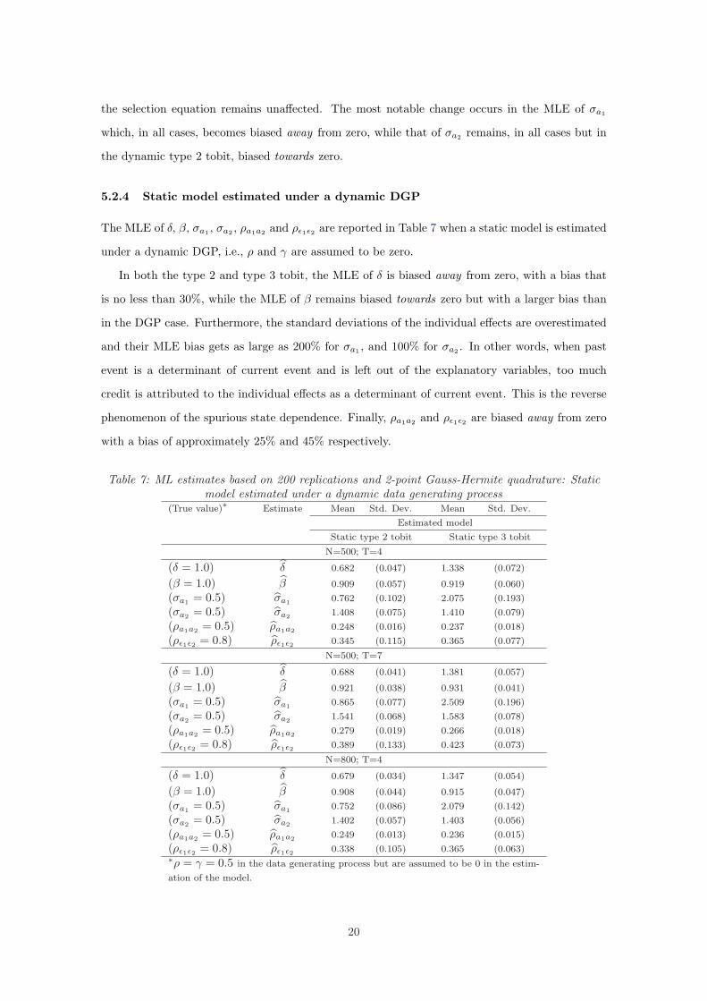
the selection equation remains unaffected. The most notable change occurs in the MLE of σa1

which, in all cases, becomes biased away from zero, while that of σa2 remains, in all cases but in

the dynamic type 2 tobit, biased towards zero.

5.2.4 Static model estimated under a dynamic DGP

The MLE of δ, β, σa1 , σa2 , ρa1a2 and ρε1ε2 are reported in Table 7 when a static model is estimated

under a dynamic DGP, i.e., ρ and γ are assumed to be zero.

In both the type 2 and type 3 tobit, the MLE of δ is biased away from zero, with a bias that

is no less than 30%, while the MLE of β remains biased towards zero but with a larger bias than

in the DGP case. Furthermore, the standard deviations of the individual effects are overestimated

and their MLE bias gets as large as 200% for σa1 , and 100% for σa2 . In other words, when past

event is a determinant of current event and is left out of the explanatory variables, too much

credit is attributed to the individual effects as a determinant of current event. This is the reverse

phenomenon of the spurious state dependence. Finally, ρa1a2 and ρε1ε2 are biased away from zero

with a bias of approximately 25% and 45% respectively.

Table 7: ML estimates based on 200 replications and 2-point Gauss-Hermite quadrature: Staticmodel estimated under a dynamic data generating process

(True value)∗ Estimate Mean Std. Dev. Mean Std. Dev.

Estimated model

Static type 2 tobit Static type 3 tobit

N=500; T=4

(δ = 1.0) δ 0.682 (0.047) 1.338 (0.072)

(β = 1.0) β 0.909 (0.057) 0.919 (0.060)

(σa1 = 0.5) σa1 0.762 (0.102) 2.075 (0.193)

(σa2 = 0.5) σa2 1.408 (0.075) 1.410 (0.079)

(ρa1a2 = 0.5) ρa1a2 0.248 (0.016) 0.237 (0.018)

(ρε1ε2 = 0.8) ρε1ε2 0.345 (0.115) 0.365 (0.077)

N=500; T=7

(δ = 1.0) δ 0.688 (0.041) 1.381 (0.057)

(β = 1.0) β 0.921 (0.038) 0.931 (0.041)

(σa1 = 0.5) σa1 0.865 (0.077) 2.509 (0.196)

(σa2 = 0.5) σa2 1.541 (0.068) 1.583 (0.078)

(ρa1a2 = 0.5) ρa1a2 0.279 (0.019) 0.266 (0.018)

(ρε1ε2 = 0.8) ρε1ε2 0.389 (0.133) 0.423 (0.073)

N=800; T=4

(δ = 1.0) δ 0.679 (0.034) 1.347 (0.054)

(β = 1.0) β 0.908 (0.044) 0.915 (0.047)

(σa1 = 0.5) σa1 0.752 (0.086) 2.079 (0.142)

(σa2 = 0.5) σa2 1.402 (0.057) 1.403 (0.056)

(ρa1a2 = 0.5) ρa1a2 0.249 (0.013) 0.236 (0.015)

(ρε1ε2 = 0.8) ρε1ε2 0.338 (0.105) 0.365 (0.063)∗ρ = γ = 0.5 in the data generating process but are assumed to be 0 in the estim-

ation of the model.

20

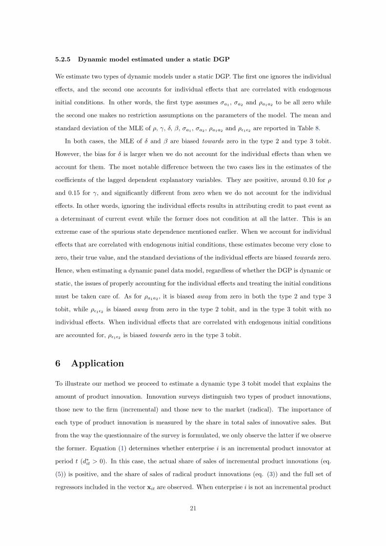
5.2.5 Dynamic model estimated under a static DGP

We estimate two types of dynamic models under a static DGP. The first one ignores the individual

effects, and the second one accounts for individual effects that are correlated with endogenous

initial conditions. In other words, the first type assumes σa1 , σa2 and ρa1a2 to be all zero while

the second one makes no restriction assumptions on the parameters of the model. The mean and

standard deviation of the MLE of ρ, γ, δ, β, σa1 , σa2 , ρa1a2 and ρε1ε2 are reported in Table 8.

In both cases, the MLE of δ and β are biased towards zero in the type 2 and type 3 tobit.

However, the bias for δ is larger when we do not account for the individual effects than when we

account for them. The most notable difference between the two cases lies in the estimates of the

coefficients of the lagged dependent explanatory variables. They are positive, around 0.10 for ρ

and 0.15 for γ, and significantly different from zero when we do not account for the individual

effects. In other words, ignoring the individual effects results in attributing credit to past event as

a determinant of current event while the former does not condition at all the latter. This is an

extreme case of the spurious state dependence mentioned earlier. When we account for individual

effects that are correlated with endogenous initial conditions, these estimates become very close to

zero, their true value, and the standard deviations of the individual effects are biased towards zero.

Hence, when estimating a dynamic panel data model, regardless of whether the DGP is dynamic or

static, the issues of properly accounting for the individual effects and treating the initial conditions

must be taken care of. As for ρa1a2 , it is biased away from zero in both the type 2 and type 3

tobit, while ρε1ε2 is biased away from zero in the type 2 tobit, and in the type 3 tobit with no

individual effects. When individual effects that are correlated with endogenous initial conditions

are accounted for, ρε1ε2 is biased towards zero in the type 3 tobit.

6 Application

To illustrate our method we proceed to estimate a dynamic type 3 tobit model that explains the

amount of product innovation. Innovation surveys distinguish two types of product innovations,

those new to the firm (incremental) and those new to the market (radical). The importance of

each type of product innovation is measured by the share in total sales of innovative sales. But

from the way the questionnaire of the survey is formulated, we only observe the latter if we observe

the former. Equation (1) determines whether enterprise i is an incremental product innovator at

period t (d∗it > 0). In this case, the actual share of sales of incremental product innovations (eq.

(5)) is positive, and the share of sales of radical product innovations (eq. (3)) and the full set of

regressors included in the vector xit are observed. When enterprise i is not an incremental product

21

Tab

le8:

ML

estim

ates

base

don

200

repl

icat

ions

and

2-po

intG

auss

-Her

mite

quad

ratu

re:

Dyn

amic

mod

eles

tim

ated

unde

ra

stat

icda

tage

nera

ting

proc

ess

(Tru

evalu

e)E

stim

ate

Mea

nStd

.D

ev.

Mea

nStd

.D

ev.

Mea

nStd

.D

ev.

Mea

nStd

.D

ev.

Est

imate

dm

odel

Dynam

icty

pe

2to

bit

Dynam

icty

pe

3to

bit

wit

hno

indiv

idualeff

ects

wit

hin

div

idualeff

ects

and

en-

wit

hno

indiv

idualeff

ects

wit

hin

div

idualeff

ects

and

en-

dogen

ous

init

ialco

ndit

ions

dogen

ous

init

ialco

ndit

ions

N=

500;T

=4

(ρ=

0.0)

ρ0.1

06

(0.0

50)

-0.0

01

(0.0

74)

0.0

99

(0.0

26)

0.0

19

(0.0

28)

(γ=

0.0)

γ0.1

58

(0.0

25)

0.0

43

(0.0

26)

0.1

47

(0.0

21)

0.0

50

(0.0

21)

(δ=

1.0)

δ0.9

10

(0.0

42)

1.0

04

(0.0

50)

0.9

85

(0.0

27)

0.9

94

(0.0

28)

(β=

1.0)

β1.0

01

(0.0

23)

1.0

05

(0.0

21)

1.0

01

(0.0

19)

1.0

07

(0.0

18)

(σa1

=0.

5)σ

a1

--

0.5

37

(0.0

80)

--

0.4

30

(0.0

69)

(σa2

=0.

5)σ

a2

--

0.4

05

(0.1

02)

--

0.3

93

(0.0

17)

(ρa1a2

=0.

5)ρ

a1a2

--

0.2

55

(0.0

65)

--

0.2

43

(0.0

19)

(ρε 1

ε 2=

0.8)

ρε 1

ε 20.6

59

(0.0

34)

0.6

60

(0.0

51)

0.6

64

(0.0

21)

0.7

09

(0.0

25)

N=

500;T

=7

(ρ=

0.0)

ρ0.1

03

(0.0

31)

-0.0

02

(0.0

44)

0.0

97

(0.0

18)

0.0

10

(0.0

19)

(γ=

0.0)

γ0.1

55

(0.0

18)

0.0

45

(0.0

17)

0.1

46

(0.0

15)

0.0

51

(0.0

13)

(δ=

1.0)

δ0.9

08

(0.0

34)

1.0

10

(0.0

41)

0.9

86

(0.0

20)

1.0

00

(0.0

21)

(β=

1.0)

β1.0

00

(0.0

16)

1.0

04

(0.0

15)

1.0

01

(0.0

13)

1.0

04

(0.0

11)

(σa1

=0.

5)σ

a1

--

0.5

93

(0.0

55)

--

0.5

28

(0.0

53)

(σa2

=0.

5)σ

a2

--

0.4

14

(0.0

15)

--

0.4

00

(0.0

14)

(ρa1a2

=0.

5)ρ

a1a2

--

0.2

93

(0.0

16)

--

0.2

63

(0.0

19)

(ρε 1

ε 2=

0.8)

ρε 1

ε 20.6

61

(0.0

25)

0.6

64

(0.0

34)

0.6

64

(0.0

16)

0.7

14

(0.0

16)

N=

800;T

=4

(ρ=

0.0)

ρ0.1

03

(0.0

40)

0.0

00

(0.0

61)

0.0

98

(0.0

19)

0.0

19

(0.0

23)

(γ=

0.0)

γ0.1

54

(0.0

12)

0.0

44

(0.0

21)

0.1

43

(0.0

16)

0.0

47

(0.0

17)

(δ=

1.0)

δ0.9

05

(0.0

34)

0.9

98

(0.0

43)

0.9

80

(0.0

21)

0.9

89

(0.0

21)

(β=

1.0)

β1.0

02

(0.0

18)

1.0

06

(0.0

17)

0.9

99

(0.0

14)

1.0

05

(0.0

13)

(σa1

=0.

5)σ

a1

--

0.5

28

(0.0

72)

--

0.4

30

(0.0

54)

(σa2

=0.

5)σ

a2

--

0.4

12

(0.0

41)

--

0.3

94

(0.0

14)

(ρa1a2

=0.

5)ρ

a1a2

--

0.2

61

(0.0

34)

--

0.2

44

(0.0

13)

(ρε 1

ε 2=

0.8)

ρε 1

ε 20.6

61

(0.0

25)

0.6

54

(0.0

42)

0.6

63

(0.0

17)

0.7

07

(0.0

18)

22

innovator, the shares of sales of incremental (dit) and radical (yit) product innovations are equal

to zero, and only the set of regressors included in the vector wit is observed.

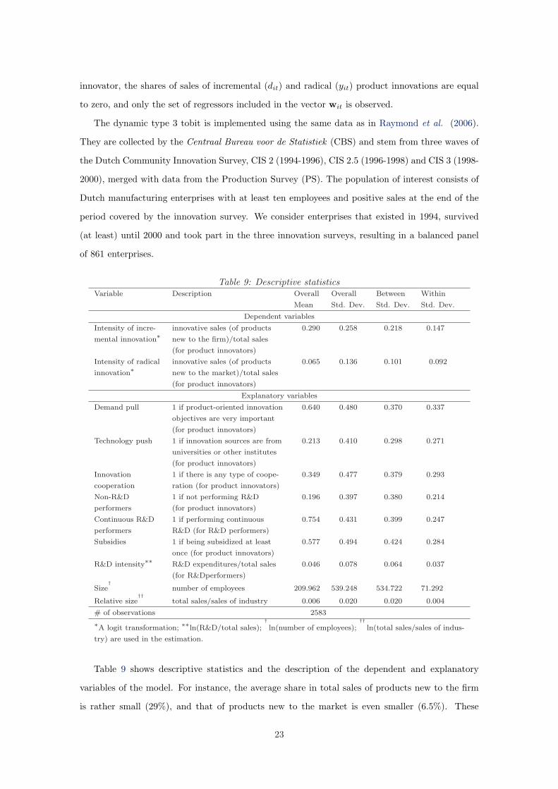
The dynamic type 3 tobit is implemented using the same data as in Raymond et al. (2006).

They are collected by the Centraal Bureau voor de Statistiek (CBS) and stem from three waves of

the Dutch Community Innovation Survey, CIS 2 (1994-1996), CIS 2.5 (1996-1998) and CIS 3 (1998-

2000), merged with data from the Production Survey (PS). The population of interest consists of

Dutch manufacturing enterprises with at least ten employees and positive sales at the end of the

period covered by the innovation survey. We consider enterprises that existed in 1994, survived

(at least) until 2000 and took part in the three innovation surveys, resulting in a balanced panel

of 861 enterprises.

Table 9: Descriptive statisticsVariable Description Overall Overall Between Within

Mean Std. Dev. Std. Dev. Std. Dev.

Dependent variables

Intensity of incre- innovative sales (of products 0.290 0.258 0.218 0.147

mental innovation∗ new to the firm)/total sales

(for product innovators)

Intensity of radical innovative sales (of products 0.065 0.136 0.101 0.092

innovation∗ new to the market)/total sales

(for product innovators)

Explanatory variables

Demand pull 1 if product-oriented innovation 0.640 0.480 0.370 0.337

objectives are very important

(for product innovators)

Technology push 1 if innovation sources are from 0.213 0.410 0.298 0.271

universities or other institutes

(for product innovators)

Innovation 1 if there is any type of coope- 0.349 0.477 0.379 0.293

cooperation ration (for product innovators)

Non-R&D 1 if not performing R&D 0.196 0.397 0.380 0.214

performers (for product innovators)

Continuous R&D 1 if performing continuous 0.754 0.431 0.399 0.247

performers R&D (for R&D performers)

Subsidies 1 if being subsidized at least 0.577 0.494 0.424 0.284

once (for product innovators)

R&D intensity∗∗ R&D expenditures/total sales 0.046 0.078 0.064 0.037

(for R&Dperformers)

Size†

number of employees 209.962 539.248 534.722 71.292

Relative size††

total sales/sales of industry 0.006 0.020 0.020 0.004

# of observations 2583

∗A logit transformation; ∗∗ln(R&D/total sales);†ln(number of employees);

††ln(total sales/sales of indus-

try) are used in the estimation.

Table 9 shows descriptive statistics and the description of the dependent and explanatory

variables of the model. For instance, the average share in total sales of products new to the firm

is rather small (29%), and that of products new to the market is even smaller (6.5%). These

23

two variables are logit-transformed in order to make them lie within the set of real numbers.13

The specification of the model is as follows. The current share in total sales of products new

to the firm is explained by the lagged share in total sales of products new to the firm, lagged

size and relative size.14 Besides lagged size, the current share in total sales of products new to

the market is explained by the lagged share in total sales of products new to the market and

dummy variables capturing demand pull, proximity to science, innovation cooperation, non-R&D

performers, subsidies, and a continuous R&D intensity variable.

Table 10 presents the estimation results of four versions of the type 3 tobit, namely a static

model with unobserved individual effects, a dynamic model with no unobserved individual effects, a

dynamic model with individual effects and endogenous initial conditions but ignoring the selection

bias, and a dynamic model with individual effects and endogenous initial conditions correcting

for selection bias.15 The hypotheses of the first three models are tested against those of the

fourth one, and rejected using a likelihood ratio test at 1% level of significance. Hence, the

preferred model is dynamic with individual effects and endogenous initial conditions correcting

for selection bias. The results suggest that, in all four versions of the model, lagged size affects

positively and significantly the current share of sales of incremental innovations. The current share

of sales of radical innovations is positively and significantly affected by R&D intensity, performing

R&D continuously, demand pull, innovation cooperation, subsidies while, ceteris paribus, non-R&D

performers are less successful than R&D performers in terms of generating innovative sales from

radical innovations. Sample selection operates through the individual effects and the idiosyncratic

errors in the static case, and only through the idiosyncratic errors in the dynamic case. In the static

case, too much of a role is attributed to the individual effects in that their standard deviations, as

well as the correlation between them, are overestimated. Finally, the coefficients associated with

the lagged dependent variables are positively and statistically significantly estimated in the three

dynamic cases. However, they are overestimated when the individual effects are not accounted for

or when the individual effects are accounted for but exogenous initial conditions are assumed.

A dynamic type 2 tobit was also estimated using information only from a binary variable,

indicating whether a firm is an incremental product innovator or not, for the selection equation13The share of sales of products new to the firm takes on the values 1 for innovators that are newly established.

They are replaced by 0.9999 in the logit transformation. Furthermore, the share of sales of products new to themarket takes on the value 0 for some incremental product innovators. They are replaced by 0.0001 in the logittransformation.

14In the innovation survey, firms are asked whether they have product and/or process innovations, or incompleteand abandoned innovation activities during the whole period under study, while size and sales are measured only atthe end of the period. Hence, all the cross-sectional studies on the determinants of innovation have this unsatisfactoryfeature of explaining the probability of being an innovator (during the whole period) by size or relative size (at theend of the period). Taking lagged size or relative size as an explanatory variable in the panel data context overcomesthis problem.

15A dynamic model with unobserved individual effects and exogenous initial conditions was also estimated. Theresults, not reported in the paper, are similar to those of the dynamic model with no individual effects.

24

Tab

le10

:M

Les

tim

ates

ofth

ety

pe3

tobi

t:5-

poin

tG

auss

-Her

mite

quad

ratu

reVari

able

Coeffi

cien

t(S

td.

Err

.)C

oeffi

cien

t(S

td.

Err

.)C

oeffi

cien

t(S

td.

Err

.)C

oeffi

cien

t(S

td.

Err

.)

Sta

tic

model

wit

hD

ynam

icm

odel

wit

h

Est

imati

on

Unobse

rved

indiv

idualeff

ects

and

endogen

ous

init

ialco

ndit

ions

ass

um

pti

on

Unobse

rved

indiv

idualeff

ects

No

unobse

rved

indiv

idualeff

ects

No

sele

ctio

nbia

sco

rrec

tion

Sel

ecti

on

bia

sco

rrec

tion

Curr

ent

share

ofsa

les

ofin

crem

enta

lpro

duct

innovati

ons(d

itin

logit)

Past

share

ofin

crem

enta

lin

nov.

sale

s(d

i,t−

1)

--

0.2

26∗∗

(0.0

20)

0.1

09∗∗

(0.0

33)

0.1

13∗∗

(0.0

33)

Lagged

size

(in

log)

0.3

74∗

(0.1

69)

0.3

04∗

(0.1

53)

0.3

51∗

(0.1

60)

0.3

54∗

(0.1

59)

Lagged

rela

tive

size

(in

log)

0.2

04†

(0.1

24)

0.0

94

(0.1

13)

0.0

70

(0.1

18)

0.0

66

(0.1

17)

Inte

rcep

t-2

.126

(1.4

79)

-1.7

93

(1.3

41)

-2.1

36

(1.4

04)

-2.1

72

(1.3

95)

Curr

ent

share

ofsa

les

ofra

dic

alpro

duct

innovati

ons(y

itin

logit)

Past

share

ofra

dic

alin

nov.

sale

s(y

i,t−

1)

--

0.2

17∗∗

(0.0

29)

0.1

14†

(0.0

63)

0.1

20∗

(0.0

60)

Lagged

size

(in

log)

0.1

39

(0.1

14)

0.0

68

(0.1

04)

0.0

31

(0.1

05)

0.0

57

(0.1

05)

R&

Din

tensi

ty(i

nlo

g)

0.2

49∗∗

(0.0

91)

0.1

99∗

(0.0

86)

0.2

17∗

(0.0

87)

0.1

93∗

(0.0

87)

Non-R

&D

per

form

ers

-1.4

15∗

(0.5

80)

-1.1

11∗

(0.5

58)

-1.0

49†

(0.5

64)

-1.0

10†

(0.5

63)

Conti

nuous

R&

Dper

form

ers

0.9

50∗∗

(0.3

01)

0.7

86∗∗

(0.2

94)

0.8

16∗∗

(0.3

00)

0.7

97∗∗

(0.2

98)

Dem

and

pull

0.6

64∗∗

(0.2

22)

0.7

02∗∗

(0.2

19)

0.7

53∗∗

(0.2

19)

0.6

88∗∗

(0.2

19)

Tec

hnolo

gy

push

-0.0

93

(0.2

54)

-0.1

62

(0.2

46)

-0.0

77

(0.2

48)

-0.1

04

(0.2

47)

Cooper

ati

on

inin

novati

on

0.5

73∗

(0.2

30)

0.5

39∗

(0.2

23)

0.5

54∗

(0.2

24)

0.5

30∗

(0.2

23)

Subsi

die

s0.6

97∗∗

(0.2

42)

0.5

62∗

(0.2

36)

0.5

32∗

(0.2

38)

0.5

55∗

(0.2

37)

Inte

rcep

t-6

.976∗∗

(0.7

31)

-5.3

53∗∗

(0.6

95)

-4.9

78∗∗

(0.7

21)

-5.1

65∗∗

(0.7

26)

Extr

apara

met

ers

Init

ialsh

are

ofin

crem

enta

lin

nov.

sale

s(d

i0)

--

--

0.1

27∗∗

(0.0

31)

0.1

23∗∗

(0.0

30)

Init

ialsh

are

ofra

dic

alin

nov.sa

les(y

i0)

--

--

0.1

22∗

(0.0

50)

0.1

25∗

(0.0

50)

σa1

1.7

79∗∗

(0.1

55)

--

1.1

39∗∗

(0.2

41)

1.1

02∗∗

(0.2

43)

σa2

1.4

52∗∗

(0.1

80)

--

0.5

93

(0.6

92)

0.5

97

(0.6

81)

σε 1

3.1

10∗∗

(0.0

84)

3.4

63∗∗

(0.0

73)

3.2

72∗∗

(0.0

98)

3.2

83∗∗

(0.0

98)

σε 2

2.9

94∗∗

(0.0

96)

3.2

47∗∗

(0.0

70)

3.1

81∗∗

(0.1

43)

3.1

79∗∗

(0.1

42)

ρa1a2

0.2

37∗

(0.1

15)

--

--

0.1

37

(0.3

37)

ρε 1

ε 20.0

73†

(0.0

40)

0.1

07∗∗

(0.0

29)

--

0.1

01∗∗

(0.0

37)

Num

ber

ofobse

rvati

ons

1722

Log-lik

elih

ood

-5978.2

55

-5915.9

79

-5910.0

01

-5904.0

49

Sig

nifi

cance

level

s:

†:10%

∗:5%

∗∗:

1%

25

and using the same equation of interest. As expected, the results (not reported in the paper) show

that the parameters of the equation of interest are (slightly) less accurately estimated but similar

to those of the type 3 tobit.

7 Conclusion

We have proposed a simple method to implement the maximum likelihood estimator of dynamic

panel data sample selection models. The method consists in writing the likelihood function condi-

tional on the individual effects which are then “integrated out” with respect to their joint normal

distribution. We have handled the two-dimensional indefinite integral involved in the likelihood

function using “two-step” Gauss-Hermite quadrature, and solved the initial conditions problem

using the approach of Wooldridge (2005). The resulting likelihood function encompasses a wide

range of likelihood functions of panel data models whose estimation can be achieved by simply

making restriction assumptions on the parameters of the dynamic panel data sample selection

model. These assumptions can be tested using a standard likelihood ratio or Wald test.

In order to assess the quality of the Gauss-Hermite quadrature, and hence that of the maximum

likelihood estimator, we have conducted a Monte Carlo study and obtained the following results.

First, under the data generating process, the maximum likelihood estimator works very well, even

for a number of integration points, in each step of the Gauss-Hermite quadrature, as small as 2.

The estimator bias of the coefficients of the lagged dependent and strictly exogenous explanatory

variables, as well as that of the standard deviations of the individual effects is very small for

a sample size as large as the one considered in the Monte Carlo study. The sample selection

terms, however, are less accurately estimated when the number of integration points is very small.

Secondly, too much of a role is attributed to the lagged dependent variables as a determinant

of the current dependent variables when either the individual effects or the correlation between

the initial outcome and the individual effects are not taken into account. Thirdly, the selection

bias really matters when the explanatory variables in the selection equation and in the equation

of interest are highly correlated, otherwise it can be safely ignored. Fourthly, when the lagged

dependent variables condition the current dependent variables and are left out of the explanatory

variables, too much of a role is attributed to the individual effects as a determinant of the current

dependent variables. Finally, when estimating a dynamic panel data model, regardless of whether

the true model is dynamic or static, the individual effects and the correlation between the initial

outcome and the individual effects must be taken into account, otherwise a situation of spurious

state dependence will arise even under its extreme form. In this latter case, credit is attributed

26

to the lagged dependent variables as a determinant of the current dependent variables while the

former do not condition at all the latter.

We have applied the method to estimate a dynamic type 3 tobit model of incremental and

radical product innovations. The estimation results confirm those of the Monte Carlo study. More

specifically, the effect of past incremental and radical product innovations on current incremental

and radical product innovations is overestimated when either the individual effects or the correla-

tion between the initial conditions and the individual effects are not accounted for. We also find

that too much importance is attributed to the individual effects as a determinant of current in-

cremental and radical product innovations when past incremental and radical product innovations

do not enter the set of explanatory variables. Finally, the estimation results of the model with no

selection bias correction are similar to those of the model with a selection bias correction, even

though the latter model is shown, using a likelihood ratio test, to be the preferred one.

Our approach can be, in a straightforward manner, extended to estimate by maximum likelihood

panel data sample selection models with more than two equations, that include a lagged dependent

explanatory variable and individual effects in each equation. For instance, our approach can handle

the estimation of dynamic panel data type 4 and type 5 tobit models with individual effects.

27

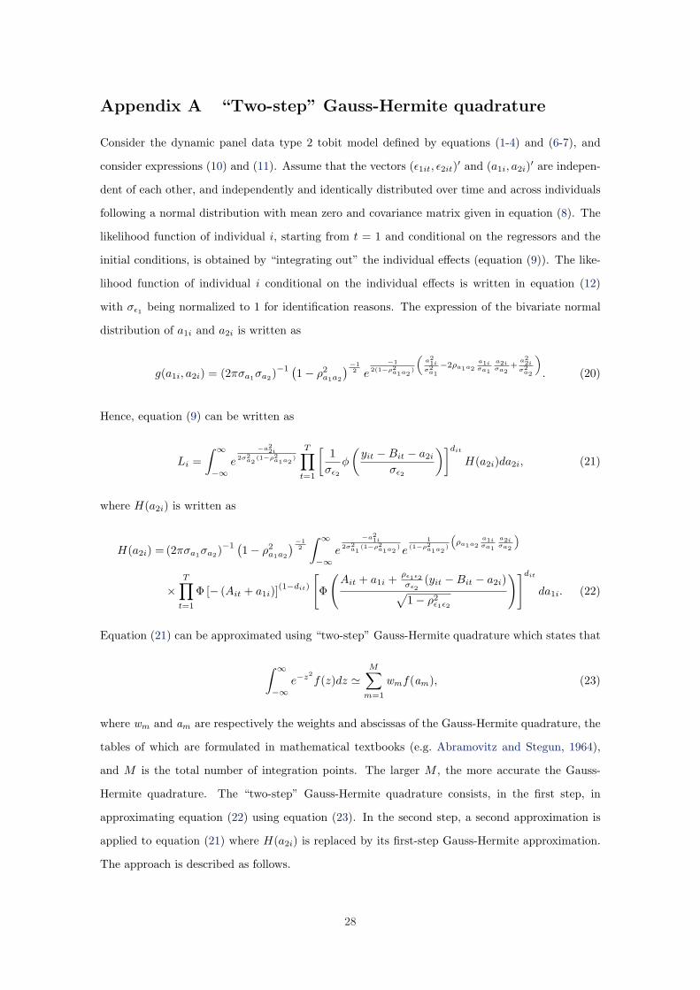
Appendix A “Two-step” Gauss-Hermite quadrature

Consider the dynamic panel data type 2 tobit model defined by equations (1-4) and (6-7), and

consider expressions (10) and (11). Assume that the vectors (ε1it, ε2it)′ and (a1i, a2i)′ are indepen-

dent of each other, and independently and identically distributed over time and across individuals

following a normal distribution with mean zero and covariance matrix given in equation (8). The

likelihood function of individual i, starting from t = 1 and conditional on the regressors and the

initial conditions, is obtained by “integrating out” the individual effects (equation (9)). The like-

lihood function of individual i conditional on the individual effects is written in equation (12)

with σε1 being normalized to 1 for identification reasons. The expression of the bivariate normal

distribution of a1i and a2i is written as

g(a1i, a2i) = (2πσa1σa2)−1 (

1− ρ2a1a2

)−12 e

−12(1−ρ2

a1a2)

„a21i

σ2a1−2ρa1a2

a1iσa1

a2iσa2

+a22i

σ2a2

«

. (20)

Hence, equation (9) can be written as

Li =∫ ∞

−∞e

−a22i

2σ2a2

(1−ρ2a1a2

)

T∏t=1

[1

σε2

φ

(yit −Bit − a2i

σε2

)]dit

H(a2i)da2i, (21)

where H(a2i) is written as

H(a2i) = (2πσa1σa2)−1 (

1− ρ2a1a2

)−12

∫ ∞

−∞e

−a21i

2σ2a1

(1−ρ2a1a2

) e1

(1−ρ2a1a2

)

“ρa1a2

a1iσa1

a2iσa2

”

×T∏

t=1

Φ [− (Ait + a1i)](1−dit)

[Φ

(Ait + a1i + ρε1ε2

σε2(yit −Bit − a2i)√

1− ρ2ε1ε2

)]dit

da1i. (22)

Equation (21) can be approximated using “two-step” Gauss-Hermite quadrature which states that

∫ ∞

−∞e−z2

f(z)dz 'M∑

m=1

wmf(am), (23)

where wm and am are respectively the weights and abscissas of the Gauss-Hermite quadrature, the

tables of which are formulated in mathematical textbooks (e.g. Abramovitz and Stegun, 1964),

and M is the total number of integration points. The larger M , the more accurate the Gauss-

Hermite quadrature. The “two-step” Gauss-Hermite quadrature consists, in the first step, in

approximating equation (22) using equation (23). In the second step, a second approximation is

applied to equation (21) where H(a2i) is replaced by its first-step Gauss-Hermite approximation.

The approach is described as follows.

28

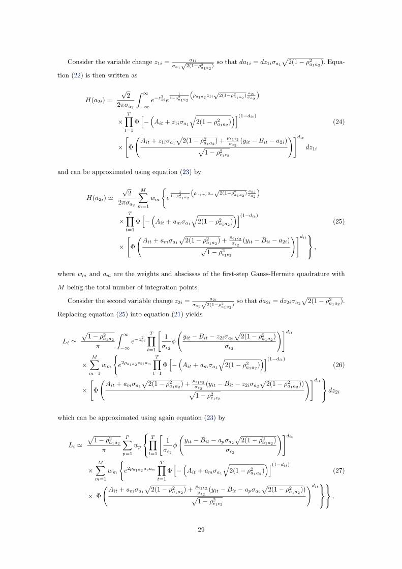
Consider the variable change z1i = a1i

σa1

√2(1−ρ2

a1a2)

so that da1i = dz1iσa1

√2(1− ρ2

a1a2). Equa-

tion (22) is then written as

H(a2i) =√

22πσa2

∫ ∞

−∞e−z2

1ie1

1−ρ2a1a2

“ρa1a2z1i

√2(1−ρ2

a1a2)

a2iσa2

”

×T∏

t=1

Φ[−

(Ait + z1iσa1

√2(1− ρ2

a1a2))](1−dit)

(24)

×[Φ

(Ait + z1iσa1

√2(1− ρ2

a1a2) + ρε1ε2

σε2(yit −Bit − a2i)√

1− ρ2ε1ε2

)]dit

dz1i

and can be approximated using equation (23) by

H(a2i) '√

22πσa2

M∑m=1

wm

e

11−ρ2

a1a2

“ρa1a2am

√2(1−ρ2

a1a2)

a2iσa2

”

×T∏

t=1

Φ[−

(Ait + amσa1

√2(1− ρ2

a1a2))](1−dit)

(25)

×[Φ

(Ait + amσa1

√2(1− ρ2

a1a2) + ρε1ε2

σε2(yit −Bit − a2i)√

1− ρ2ε1ε2

)]dit ,

where wm and am are the weights and abscissas of the first-step Gauss-Hermite quadrature with

M being the total number of integration points.

Consider the second variable change z2i = a2i

σa2

√2(1−ρ2

a1a2)

so that da2i = dz2iσa2

√2(1− ρ2

a1a2).

Replacing equation (25) into equation (21) yields

Li '√

1− ρ2a1a2

π

∫ ∞

−∞e−z2

2i

T∏t=1

[1

σε2

φ

(yit −Bit − z2iσa2

√2(1− ρ2

a1a2)

σε2

)]dit

×M∑

m=1

wm

e2ρa1a2z2iam

T∏t=1

Φ[−

(Ait + amσa1

√2(1− ρ2

a1a2))](1−dit)

(26)

×[Φ

(Ait + amσa1

√2(1− ρ2

a1a2) + ρε1ε2

σε2(yit −Bit − z2iσa2

√2(1− ρ2

a1a2))

√1− ρ2

ε1ε2

)]dit dz2i

which can be approximated using again equation (23) by

Li '√

1− ρ2a1a2

π

P∑p=1

wp

T∏t=1

[1

σε2

φ

(yit −Bit − apσa2

√2(1− ρ2

a1a2)

σε2

)]dit

×M∑

m=1

wm

e2ρa1a2apam

T∏t=1

Φ[−

(Ait + amσa1

√2(1− ρ2

a1a2))](1−dit)

(27)

× Φ

(Ait + amσa1

√2(1− ρ2

a1a2) + ρε1ε2

σε2(yit −Bit − apσa2

√2(1− ρ2

a1a2))

√1− ρ2

ε1ε2

)dit

,

29

where wp and ap are the weights and abscissas of the second-order Gauss-Hermite quadrature with

P being the total number of integration points.

Using equations (9), (13), (14) and (20), the random-effects individual likelihood function of

the type 3 tobit can be derived similarly to yield equation (16).

30

References

Abramovitz M, Stegun I. 1964. Handbook of Mathematical Functions with Formulas, Graphs, and

Mathematical Tables. National Bureau of Standards Applied Mathematics, US Government

Printing Office: Washington, D.C.

Ai C, Chen C. 1992. Estimation of a fixed effects bivariate censored regression model. Economics

Letters 40: 403–406.

Amemiya T. 1984. Tobit models: A survey. Journal of Econometrics 24: 3–62.

Arellano M, Honore B. 2001. Panel data models: Some recent developments. In Handbook of

Econometrics, Heckman JJ, Leamer E (eds). North Holland: Amsterdam.

Askildsen JE, Baltagi BH, Holmas TH. 2003. Wage policy in the health care sector: A panel data

analysis of nurses’ labour supply. Health Economics 12: 705–719.

Butler JS, Moffitt R. 1982. A computationally efficient quadrature procedure for the one-factor

multinomial probit model. Econometrica 50: 761–764.

Chamberlain G. 1980. Analysis of covariance with qualitative data. Review of Economic Studies

47: 225–238.

Dustmann Christian, Rochina-Barrachina Marıa Engracia. 2000. Selection correction in panel data

models: An application to labour supply and wages. IZA Discussion Paper No. 162.

Gayle G-L, Viauroux C. 2007. Root-n consistent semiparametric estimators of a dynamic panel-

sample-selection model. Journal of Econometrics . Forthcoming.

Greene W. 2004a. The behaviour of the maximum likelihood estimator of limited dependent

variable models in the presence of fixed effects. Econometrics Journal 7: 98–119.

Greene W. 2004b. Convenient estimators for the panel probit model: Further results. Empirical

Economics 29: 21–47.

Guilkey DK, Murphy JL. 1993. Estimation and testing in the random effects probit model. Journal

of Econometrics 59: 301–317.

Hausman JA, Wise DA. 1979. Attrition bias in experimental and panel data: The Gary income

maintenance experiment. Econometrica 47: 455–474.

Heckman JJ. 1979. Sample selection bias as a specification error. Econometrica 47: 153–162.

31

Heckman JJ. 1981a. Heterogeneity and state dependence. In Studies in Labor Markets, Rosen S

(ed). University of Chicago Press.

Heckman JJ. 1981b. The incidental parameters problem and the problem of initial conditions in

estimating a discrete time-discrete data stochastic process. In Structural Analysis of Discrete

Data with Econometric Applications, Manski CF, McFadden D (eds). MIT Press: Cambridge,

MA.

Heckman JJ, MaCurdy TE. 1980. A life cycle model of female labour supply. Review of Economic

Studies 47: 47–74.

Honore BE, Kyriazidou E. 2000. Estimation of tobit-type models with individual specific effects.

Econometric Reviews 19: 341–366.

Hsiao C. 2003. Analysis of Panel Data. 2nd edn. Cambridge University Press.

Kyriazidou E. 1997. Estimation of a panel data sample selection model. Econometrica 65: 1335–

1364.

Kyriazidou E. 2001. Estimation of dynamic panel data sample selection models. Review of Eco-

nomic Studies 68: 543–572.

Lancaster T. 2000. The incidental parameter problem since 1948. Journal of Econometrics 95:

391–413.

Lee M-J. 2001. First-difference estimator for panel censored-selection models. Economics Letters

70: 43–49.

Magnac T. 2004. Panel binary variables and sufficiency: Generalizing conditional logit. Econo-

metrica 72: 1859–1876.

Neyman J, Scott EL. 1948. Consistent estimates based on partially consistent observations. Econo-

metrica 16: 1–32.

Nijman T, Verbeek M. 1992. Nonresponse in panel data: The impact on estimates of a life cycle

consumption function. Journal of Applied Econometrics 7: 243–257.

Rabe-Hesketh S, Skrondal A, Pickles A. 2005. Maximum likelihood estimation of limited and

discrete dependent variable models with nested random effects. Journal of Econometrics 128:

301–323.

32

Raymond W. 2007. The dynamics of innovation and firm performance: An econometric panel data

analysis. Ph.D. thesis, Maastricht University. forthcoming.

Raymond W, Mohnen P, Palm F, Schim van der Loeff S. 2006. Persistence of innovation in Dutch

manufacturing: Is it spurious? CESifo Working Paper No. 1681.

Ridder G. 1990. Attrition in multi-wave panel data. In Panel Data and Labor Market Studies,

Hartog J, Ridder G, Theeuwes J (eds). North-Holland, Amsterdam.

Rochina-Barrachina ME. 1999. A new estimator for panel data sample selection models. Annales

d’Economie et de Statistiques 55-56: 153–182.

Semykina A, Wooldridge JM. 2005. Estimating panel data models in the presence of endogeneity

and selection: Theory and application. unpublished working paper, Michigan State University.

Vella F. 1998. Estimating models with sample selection bias: A survey. The Journal of Human

Resources 33: 127–169.

Vella F, Verbeek M. 1999. Two-step estimation of panel data models with censored endogenous

variables and selection bias. Journal of Econometrics 90: 239–263.

Verbeek M. 1990. On the estimation of a fixed effects model with selectivity bias. Economic Letters

34: 267–270.

Wooldridge JM. 1995. Selection corrections for panel data models under conditional mean inde-

pendence assumptions. Journal of Econometrics 68: 115–132.

Wooldridge JM. 2005. Simple solutions to the initial conditions problem in dynamic nonlinear

panel data models with unobserved heterogeneity. Journal of Applied Econometrics 20: 39–54.

Zabel JE. 1992. Estimating fixed and random effects models with selectivity. Economics Letters

40: 269–272.

33

The UNU-MERIT WORKING Paper Series

2007-01 Developing science, technology and innovation indicators: what we can

learn from the past by Christopher Freeman & Luc Soete 2007-02 The impact of innovation activities on productivity and firm growth:

evidence from Brazil by Micheline Goedhuys 2007-03 Estimations of US debt dynamics: Growth cum debt and the savings glut in

Kouri’s model by Thomas Ziesemer 2007-04 States and Firms on the Periphery: The Challenges of a Globalising World

by Gabriel R.G. Benito & Rajneesh Narula 2007-05 How Do Consumers Make Choices? A Summary of Evidence from

Marketing and Psychology by Zakaria Babutsidze 2007-06 Inter-firm Technology Transfer: Partnership-embedded Licensing or

Standard Licensing Agreements? by John Hagedoorn, Stefanie Lorenz-Orlean & Hans Kranenburg

2007-07 The Behavior of the Maximum Likelihood Estimator of Dynamic Panel

Data Sample Selection Models by Wladimir Raymond, Pierre Mohnen, Franz Palm & Sybrand Schim van der Loeff