Full text - NKS - Nordic Nuclear Safety Research

Nordisk kernesikkerhedsforskningNorrænar kjarnöryggisrannsóknir

Pohjoismainen ydinturvallisuustutkimusNordisk kjernesikkerhetsforskning

Nordisk kärnsäkerhetsforskningNordic nuclear safety research

NKS-236 ISBN 978-87-7893-308-9

CFD and FEM modeling of PPOOLEX experiments

Timo Pättikangas, Jarto Niemi and Antti Timperi

VTT Technical Research Centre of Finland

January 2011

Abstract Large-break LOCA experiment performed with the PPOOLEX experimen-tal facility is analysed with CFD calculations. Simulation of the first 100 seconds of the experiment is performed by using the Euler-Euler two-phase model of FLUENT 6.3. In wall condensation, the condensing water forms a film layer on the wall surface, which is modelled by mass transfer from the gas phase to the liquid water phase in the near-wall grid cell. The direct-contact condensation in the wetwell is modelled with simple correlations. The wall condensation and direct-contact condensation models are implemented with user-defined functions in FLUENT. Fluid-Structure Interaction (FSI) calculations of the PPOOLEX experiments and of a realistic BWR containment are also presented. Two-way coupled FSI calculations of the experiments have been numerically unstable with explicit coupling. A linear perturbation method is therefore used for preventing the numerical instability. The method is first validated against numerical data and against the PPOOLEX experiments. Preliminary FSI calculations are then performed for a realistic BWR containment by modeling a sector of the containment and one blowdown pipe. For the BWR containment, one- and two-way coupled calculations as well as calculations with LPM are carried out.

Key words Large-break LOCA, Condensation pool, pressure suppression pool, BWR, CFD, fluid-structure interactions, FSI NKS-236 ISBN 978-87-7893-308-9 Electronic report, January 2011 NKS Secretariat NKS-776 P.O. Box 49 DK - 4000 Roskilde, Denmark Phone +45 4677 4045 Fax +45 4677 4046 www.nks.org e-mail [email protected]

RESEARCH REPORT VTTR0218710

CFD and FEM modeling ofPPOOLEX experimentsAuthors: Timo Pättikangas, Jarto Niemi and Antti Timperi

Confidentiality: Public


2 (39)

Contents

Nomenclature ..............................................................................................................3

1 Introduction.............................................................................................................4

2 PPOOLEX experimental facility ..............................................................................5

3 CFD model for condensation..................................................................................63.1 Wall condensation...........................................................................................63.2 Direct contact condensation............................................................................8

4 CFD modelling of the experiment WLL0502.......................................................10

5 Fluidstructure interaction calculations .................................................................205.1 Orderofmagnitude analysis.........................................................................205.2 Comparison with twoway coupling...............................................................225.3 Comparison with PPOOLEX experiment.......................................................235.4 Modeling of realistic BWR containment ........................................................26

6 Summary and conclusions....................................................................................38

References ................................................................................................................39


3 (39)

Nomenclature

Latin letters

c speed of soundCp specific heat capacity (J/kg)g acceleration of gravityg acceleration of gravity vectorh enthalpy (J/kg)htc heat transfer coefficient (W/m2K)L length

"m& mass flux density (kg/m2s)p pressure

"Q heat flux density (W/m2)t timeT temperatureT viscous stress tensorV velocityV velocity vectorw wall displacementw molecular weighty mole fractionY mass fraction

Greek letters

molecular viscositydensity

Subscripts

air air species component of the gas phasei interfacegas gas phase in the EulerEuler modelsat saturated statesteam vapour species component of the gas phasetot totalwater liquid phase in the EulerEuler model


4 (39)

1 Introduction

In boiling water reactors (BWR), the major function of the containment system is to protectthe environment if a lossofcoolant accident (LOCA) should occur. The containment isdesigned to accommodate the loads generated in hypothetical accidents, such as suddenrupture of a main steam line. In such an accident, a large amount of steam is suddenlyreleased in the containment. An essential part of the pressure suppression containment is awater pool, where condensation of released steam occurs.

In a BWR, the pressure suppression containment typically consists of a drywell and a wetwellwith a water pool. In a hypothetical LOCA, steam and air flow from the drywell through avent pipe to the wetwell, where the outlet of the vent pipe is submerged in the water pool. Inearly part of the accident, mainly noncondensable air or nitrogen flows through the vent pipeinto the wetwell. Then, the volume fraction of vapour increases in the gas mixture. When allthe noncondensable gas from the drywell is blown into the wetwell, the blowdown consistsof pure vapour. The pressure suppression pool changes this large volume of vapour to a smallvolume of water (Lahey and Moody, 1993).

PPOOLEX test facility is a scaleddown model of a pressure suppression containment of aBWR (Laine and Puustinen, 2009). The pressurized PPOOLEX vessel shown in Figure 1consists of a drywell compartment and a wetwell compartment with a water pool. Thecompartments are connected with a vent pipe, whose outlet is submerged in water pool in thewetwell. In experiments, vapour is generated in a steam generator and blown into the drywell.

In the PPOOLEX experiment WLL0502, vapour was blown into the preheated drywellcompartment of the facility. The vapour jet hit the opposite wall of the drywell, where wallcondensation occurred. The temperature of the wall structures of the dry well rose and heatwas conducted through uninsulated walls to the ambient laboratory. When the pressure in thedrywell increased, the mixture of air and vapour started flowing through the vent pipe into thewater pool of the wetwell. The vent pipe was cleared of water and large gas bubbles formed atthe pipe outlet with a frequency of about one hertz. The volume fraction of vapour in thedrywell increased and directcontact condensation at the outlet of the vent pipe becamesignificant.

In the present work, a computational fluid dynamics (CFD) simulation of the first 100seconds of the experiment is performed by using the EulerEuler twophase model ofFLUENT 6.3. In the model, the gas phase consists of air and vapour species components. Inwall condensation, the condensing water forms a film layer on the wall surface, which ismodelled by mass transfer from the gas phase to the liquid water phase in the nearwall gridcell. The heat transfer from the gas phase through the water film to the wall is resolved. Thedirectcontact condensation in the wetwell is modelled with simple correlations. The wallcondensation and directcontact condensation models are implemented with userdefinedfunctions in FLUENT.

FluidStructure Interaction (FSI) calculations of the PPOOLEX experiments and of a realisticBWR containment are also presented. In the FSI calculations, the motion of the structures istaken into account when the pressure loads on the structures are calculated. StarCD is usedfor CFD calculations and Abaqus for structural analysis. The external MpCCI code is used forcoupling the CFD and structural analysis codes. Twoway coupled FSI calculations of theexperiments have been numerically unstable with explicit coupling. A linear perturbation


5 (39)

method (LPM) (Huber et al., 1979; Sonin, 1980; Timperi, 2009) is therefore used forpreventing the numerical instability. The method is first validated against numerical data andagainst the PPOOLEX experiments. Preliminary FSI calculations are then performed for arealistic BWR containment by modelling a sector of the containment and one blowdown pipe.For the BWR containment, one and twoway coupled calculations as well as calculationswith LPM are carried out.

In Section 2, the PPOOLEX facility and the experiment WLL0502 are described. The twophase CFD models for condensation are described in Section 3. In Section 4, the CFD resultsfor the experiment WLL0502 are presented and compared to the measurements. InSection 5, the FSI calculations are presented the LPM method is described. The resultsobtained with the LPM method are compared to results obtained with full twoway couplingof the CFD and FEM codes. First results on modelling a realistic BWR containment arepresented. Finally, Section 6 contains summary and discussion.

2 PPOOLEX experimental facility

PPOOLEX is an about 31 m3 pressurized cylindrical vessel with a height of 7.45 meters and adiameter of 2.4 meters. The volume of the drywell compartment is 13.3 m3 and the volume ofthe wetwell compartment is 17.8 m3. The DN200 (∅219.1 × 2.5 mm) vent pipe is positionedin a nonaxisymmetric location 300 mm away from the centre of the facility. The water levelin the beginning of the experiments was 2.14 m from the bottom of the pool. Thesubmergence depth of the DN200 vent pipe was 1.05 m, which corresponds to a hydrostaticpressure of about 10.2 kPa at the vent pipe outlet. The PPOOLEX facility is shown inFigure 1.

Figure 1. Pressure (Pn) and temperature (Tn) measurements in the PPOOLEX pressurizedtest facility at Lappeenranta University of Technology (Laine and Puustinen, 2008). On theright, the surface mesh and the outer wall temperature (C) at time t = 0 are shown.


6 (39)

In the experiments, pure vapour was blown into the drywell compartment of the PPOOLEXfacility through the horizontal DN200 pipe. Vapour was obtained from the PACTEL steamgenerator connected to the DN200 pipe with a DN50 pipe. The mass flow rate of vapour intothe drywell was measured with a vortex meter located in the DN50 line. In addition, thetemperature of vapour was measured in the inlet plenum. The measured mass flow rate andtemperature were used as boundary conditions in the CFD simulations.

Three different condensation phenomena occur in the experiments. First, some bulkcondensation of vapour may occur, when vapour flows from the DN50 pipe through theDN200 inlet plenum into the drywell. Second, part of the vapour is condensed on the walls ofthe drywell. The wall condensation is determined by the initial wall temperature in thedrywell and by the heat transfer through the walls of the drywell to the laboratory. Third,directcontact condensation occurs in the water pool of the wetwell, when vapour flows fromthe drywell to the wetwell.

3 CFD model for condensation

The EulerEuler model of FLUENT 6.3 was used in modelling the experiment. In the EulerEuler model, the conservation equations of mass, momentum and enthalpy are solved for thegas phase and liquid phase. The gas phase is wet air, which consists of two speciescomponents: dry air and vapour. Transport equation is solved for the mass fraction of air Yairin the gas phase and the mass fraction of vapour is Ysteam = 1 –Yair. Gas phase is treated as acompressible ideal gas, where wall condensation, directcontact condensation and bulkcondensation are modelled with userdefined functions of FLUENT.

3.1 Wall condensation

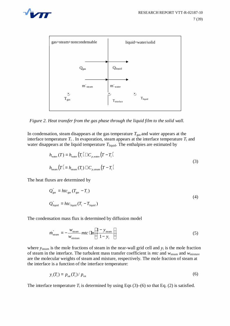
The idea of the diffusive wall condensation model is illustrated in Fig. 2, where the mass andenergy balances at the gasliquid interface are shown. In condensation or evaporation, themass balance reads

"water

"steam mm && = (1)

where "steamm& is the mass sink or source in the gas phase and "

waterm& is the mass source or sinkin the liquid phase. The energy balance at the interface is

)()( waterwater"water

"liquidsteamsteam

"steam

"gas ThmQThmQ && +=+ (2)

where Tsteam and Twater depend on the direction of the mass transfer (i.e., condensation orevaporation)


7 (39)

Figure 2. Heat transfer from the gas phase through the liquid film to the solid wall.

In condensation, steam disappears at the gas temperature Tgas and water appears at theinterface temperature Ti . In evaporation, steam appears at the interface temperature Ti andwater disappears at the liquid temperature Tliquid. The enthalpies are estimated by

( ) ( )iwater,iwaterwater )( TTCThTh p −+=

( ) ( )isteam,isteamsteam )( TTCThTh p −+=(3)

The heat fluxes are determined by

)( igasgas"gas TThtcQ −=

)( liquidiliquid"liquid TThtcQ −=

(4)

The condensation mass flux is determined by diffusion model

−

−⋅−=

i

steam

mixture

steam"steam 1

1ln

yy

mtcww

m& (5)

where ysteam is the mole fractions of steam in the nearwall grid cell and yi is the mole fractionof steam in the interface. The turbulent mass transfer coefficient is mtc and wsteam and wmixtureare the molecular weights of steam and mixture, respectively. The mole fraction of steam atthe interface is a function of the interface temperature:

totisatii /)()( pTpTy = (6)

The interface temperature Ti is determined by using Eqs (3)–(6) so that Eq. (2) is satisfied.

gas=steam+noncondensables

liquid=water/solid

Qgas Qliquid

Tgas Tliquid

steam water

Tinterface


8 (39)

3.2 Direct contact condensation

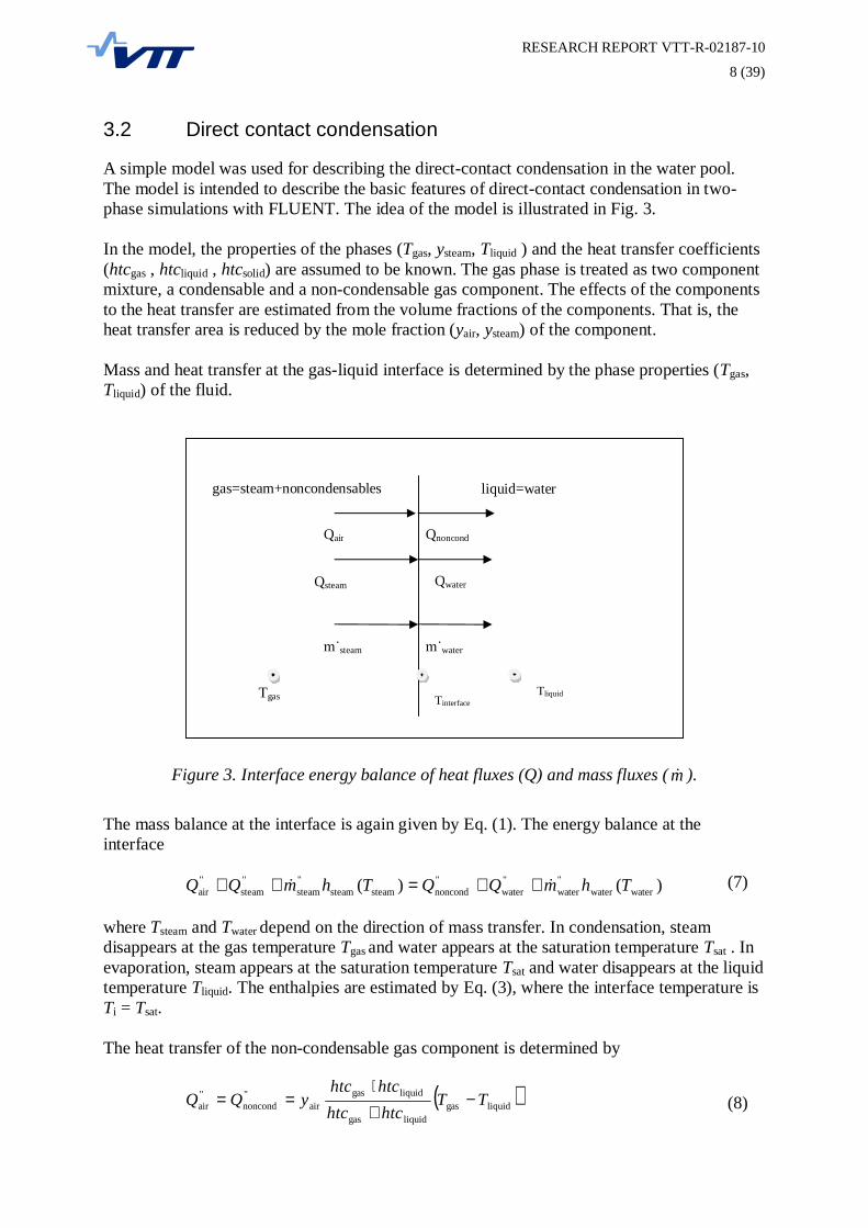
A simple model was used for describing the directcontact condensation in the water pool.The model is intended to describe the basic features of directcontact condensation in twophase simulations with FLUENT. The idea of the model is illustrated in Fig. 3.

In the model, the properties of the phases (Tgas, ysteam, Tliquid ) and the heat transfer coefficients(htcgas , htcliquid , htcsolid) are assumed to be known. The gas phase is treated as two componentmixture, a condensable and a noncondensable gas component. The effects of the componentsto the heat transfer are estimated from the volume fractions of the components. That is, theheat transfer area is reduced by the mole fraction (yair, ysteam) of the component.

Mass and heat transfer at the gasliquid interface is determined by the phase properties (Tgas,Tliquid) of the fluid.

Figure 3. Interface energy balance of heat fluxes (Q) and mass fluxes ( m& ).

The mass balance at the interface is again given by Eq. (1). The energy balance at theinterface

)()( waterwater"water

"water

"noncondsteamsteam

"steam

"steam

"air ThmQQThmQQ && ++=++ (7)

where Tsteam and Twater depend on the direction of mass transfer. In condensation, steamdisappears at the gas temperature Tgas and water appears at the saturation temperature Tsat . Inevaporation, steam appears at the saturation temperature Tsat and water disappears at the liquidtemperature Tliquid. The enthalpies are estimated by Eq. (3), where the interface temperature isTi = Tsat.

The heat transfer of the noncondensable gas component is determined by

( )liquidgasliquidgas

liquidgasair

"noncond

"air TT

htchtchtchtc

yQQ −+

⋅== (8)

gas=steam+noncondensables liquid=water

Qsteam Qwater

Tgas Tliquid

Qnoncond

steam water

Qair

Tinterface


9 (39)

The condensation or evaporation is determined by the saturation temperature of thecondensable gas component:

)( steamsatsat pTT = (9)

The heat fluxes are

( )satgasgassteam"steam TThtcyQ −⋅= (10)

( )liquidsatliquidsteam"water TThtcyQ −⋅= (11)

When condensation occurs, i.e., "steam

"water QQ > , the mass flux of steam is

( )satgasgas,fg

"steam

"water"

steam TTChQQm

p −+−

=& (12)

where the latent heat is ( )satwatersatsteamfg )( ThThh −= . When evaporation occurs, the mass fluxof steam is

( )satliquidliquid,fg

"steam

"water"

steam TTChQQm

p −−−

=& (13)

In the FLUENT model, a volumetric mass transfer rate is needed, which is obtained bymultiplying the mass flux by area density. The area density is estimated by α∇=ai , whereα is the void fraction.

In the present simulation, the heat transfer coefficient of gas has a constant value of htcgas =1000. The heat transfer coefficient for liquid is calculated from the correlation of Chen andMayinger: 5.07.0

liquid PrRe185.0=htc .


10 (39)

4 CFD modelling of the experiment WLL0502

The CFD mesh of the PPOOLEX facility consists of 135 000 hexahedral grid cells. Thesurface mesh is shown in Fig. 1. The QUICK scheme was used for the spatial discretization ofthe volume fraction equation and the second order upwind scheme for other variables. Thefirst order implicit method was used for the time discretization with a time step of ∆t = 0.01 s.The gas phase was modelled as compressible ideal gas, and the floating operating pressureoption of FLUENT was used.

In the PPOOLEX experiment WLL0502, vapour was blown into the preheated drywellcompartment of the facility. The initial temperature of the drywell was about 65 °C, and theinitial temperature of the water pool in the wetwell compartment was about 20 °C. The initialmole fraction of vapour in the gas phase was ysteam = 0.01. Temperature of the ambientlaboratory was 25 °C. The heat transfer coefficient from the uninsulated wall to the ambientlaboratory was assumed to be 4.53 W/m2K, and the emissivity of the outer wall was assumedto be ε = 0.3. The thickness of the steel wall of the drywell was 8 mm.

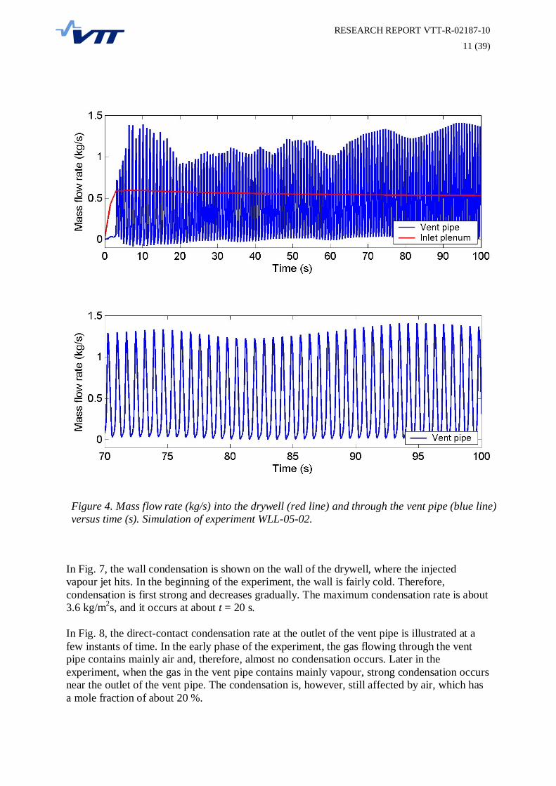
In the experiment, a gas jet was injected into the drywell through the inlet plenum. In the CFDcalculation, the gas was almost pure vapour containing a mass fraction of one percent of air.The maximum mass flow rate of the jet was 0.54 kg/s, and the vapour temperature in the inletplenum was about 140 °C. The mass flow rate into the drywell is shown in Fig. 4.

When the pressure in the drywell increases, the water plug in the vent pipe starts movingdownwards. The vent pipe is cleared at time t = 6 s and the first bubble is formed at the outletof the vent pipe in the water pool. After this, new bubbles are formed with a period of about0.72 s. The periodic formation of bubbles can be clearly seen in the mass flow rate throughthe vent pipe that is shown in Fig. 4. When bubbles are detached from the vent outlet, themass flow rate in the vent pipe becomes for awhile almost zero or is even reversed.

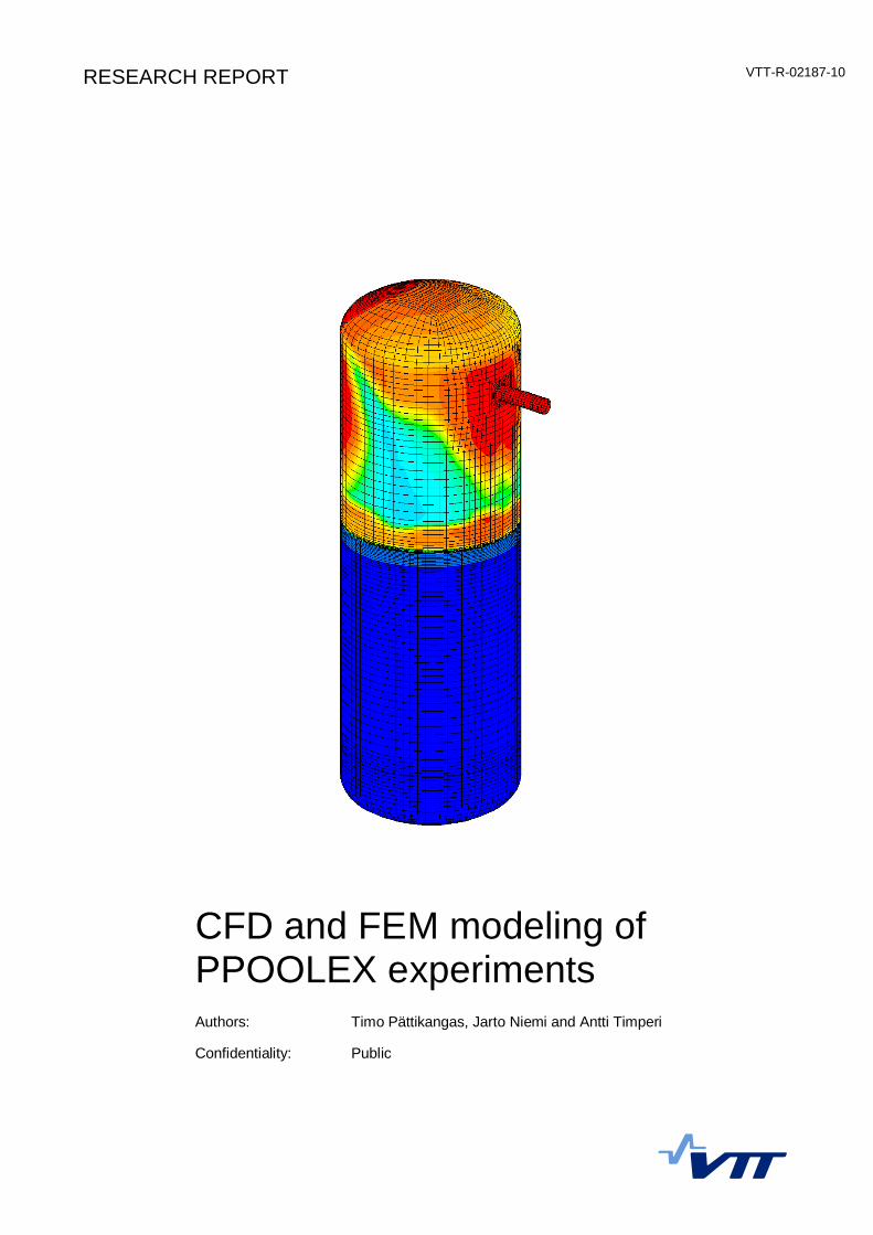
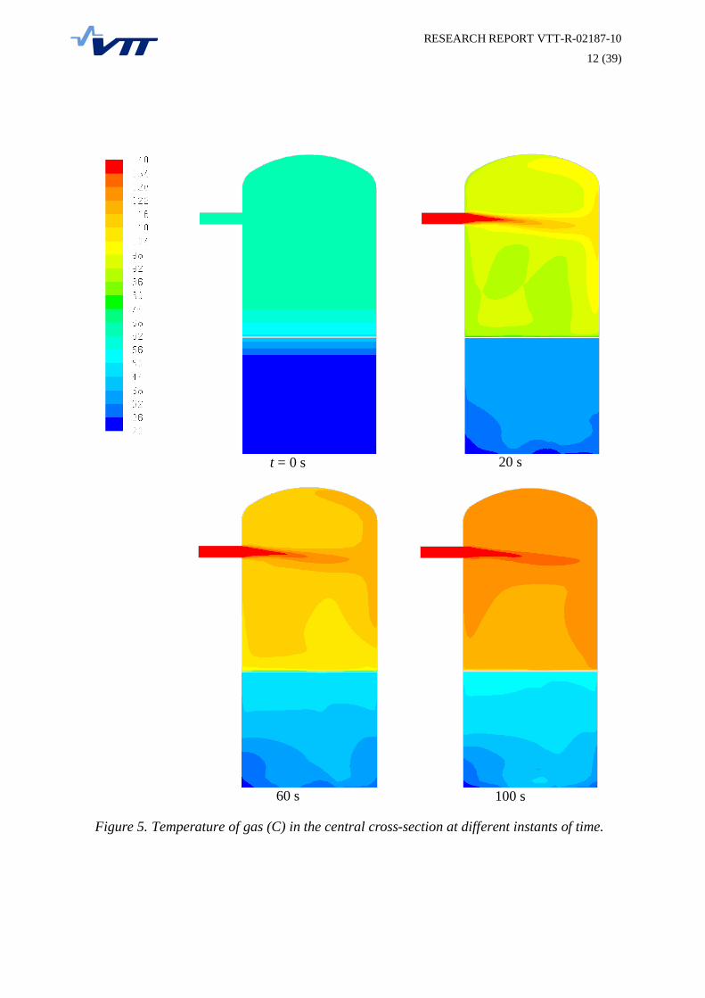
In Fig. 5, the temperature of the gas phase is shown at a few instants of time. The initialtemperature of the preheated drywell is somewhat stratified. Some heat conduction occurredthrough the floor of the drywell to the top part of the wetwell. The temperature was initializedto correspond to the measured temperatures at time t = 0. The initial temperature of the outerwall is shown in Fig. 1.

The hot steam jet injected into the drywell is seen in Fig. 5. The temperature of the drywellrises during the first 100 s to about 120 °C. The temperature of the outer wall at time t = 100 sis shown on the front cover of this report. The temperature scale is from 20 °C to 120 °C.

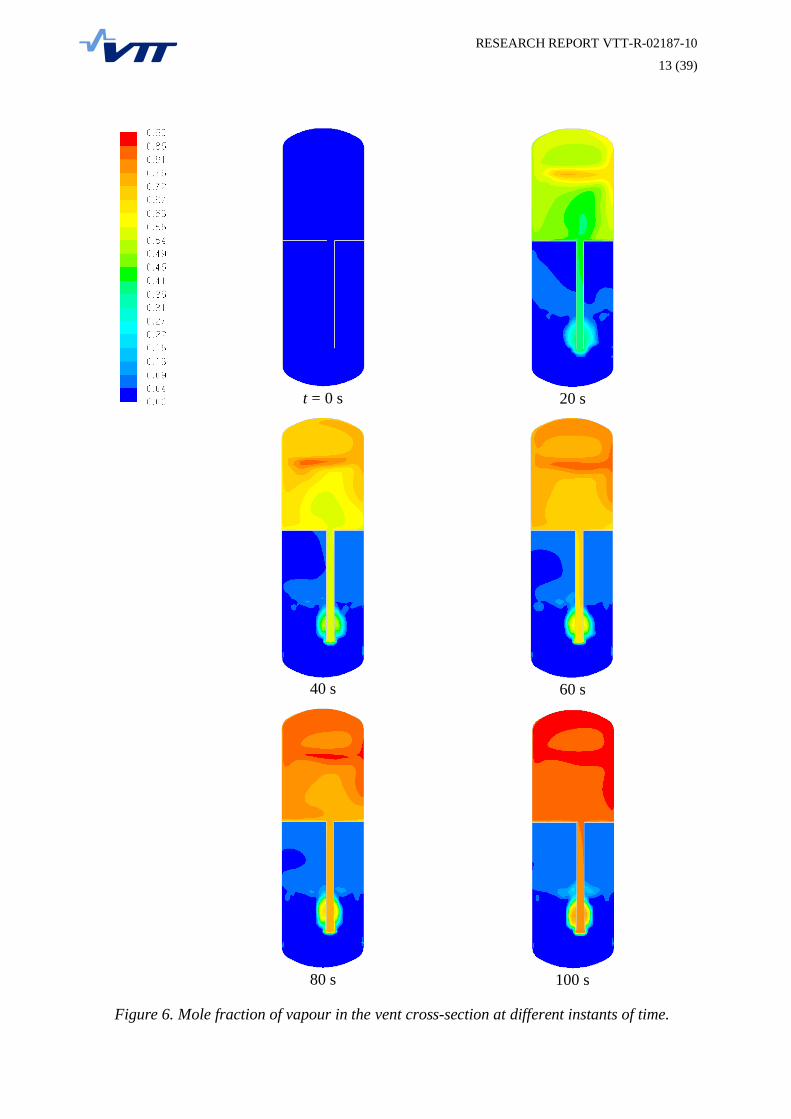
In Fig. 6, the mole fraction of vapour in the gas phase is shown. The mole fraction of vapourincreases rapidly from its initial value of one percent. At time t = 100 s, the mole fraction ofvapour is about 90% in the drywell. At this time, the gas flowing through the vent pipe intothe water pool contains almost 80 % of vapour. Strong condensation of vapour occurs on thewalls of the drywell and on the walls of the vent pipe that is submerged in cold water.


11 (39)

Figure 4. Mass flow rate (kg/s) into the drywell (red line) and through the vent pipe (blue line)versus time (s). Simulation of experiment WLL0502.

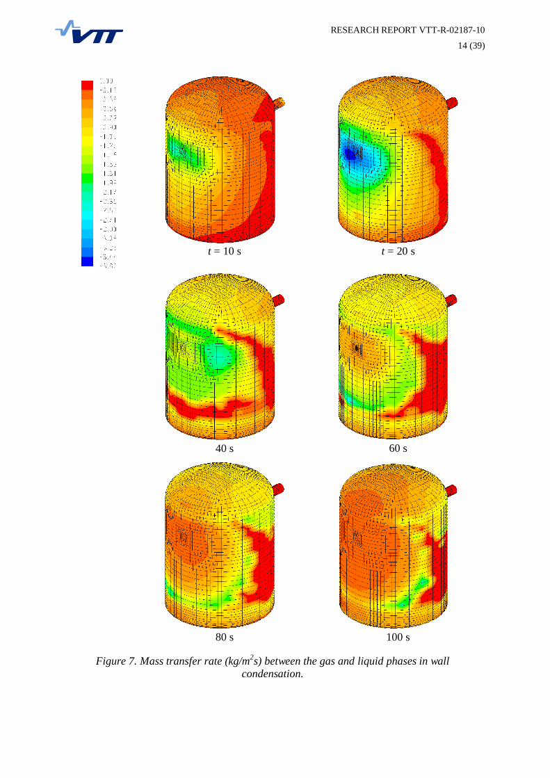
In Fig. 7, the wall condensation is shown on the wall of the drywell, where the injectedvapour jet hits. In the beginning of the experiment, the wall is fairly cold. Therefore,condensation is first strong and decreases gradually. The maximum condensation rate is about3.6 kg/m2s, and it occurs at about t = 20 s.

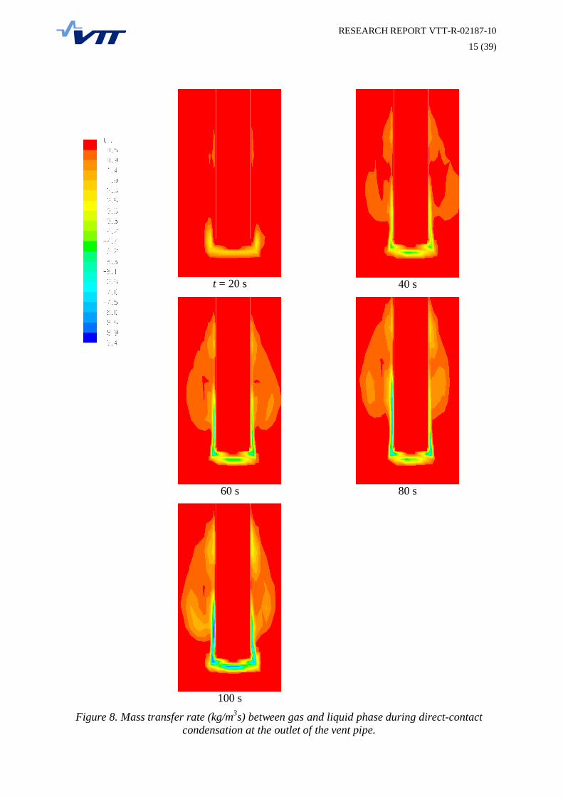
In Fig. 8, the directcontact condensation rate at the outlet of the vent pipe is illustrated at afew instants of time. In the early phase of the experiment, the gas flowing through the ventpipe contains mainly air and, therefore, almost no condensation occurs. Later in theexperiment, when the gas in the vent pipe contains mainly vapour, strong condensation occursnear the outlet of the vent pipe. The condensation is, however, still affected by air, which hasa mole fraction of about 20 %.


12 (39)

t = 0 s 20 s

60 s 100 s

Figure 5. Temperature of gas (C) in the central crosssection at different instants of time.


13 (39)

t = 0 s 20 s

40 s 60 s

80 s 100 s

Figure 6. Mole fraction of vapour in the vent crosssection at different instants of time.


14 (39)

t = 10 s t = 20 s

40 s 60 s

80 s 100 s

Figure 7. Mass transfer rate (kg/m2s) between the gas and liquid phases in wallcondensation.


15 (39)

t = 20 s 40 s

60 s 80 s

100 s

Figure 8. Mass transfer rate (kg/m3s) between gas and liquid phase during directcontactcondensation at the outlet of the vent pipe.


16 (39)

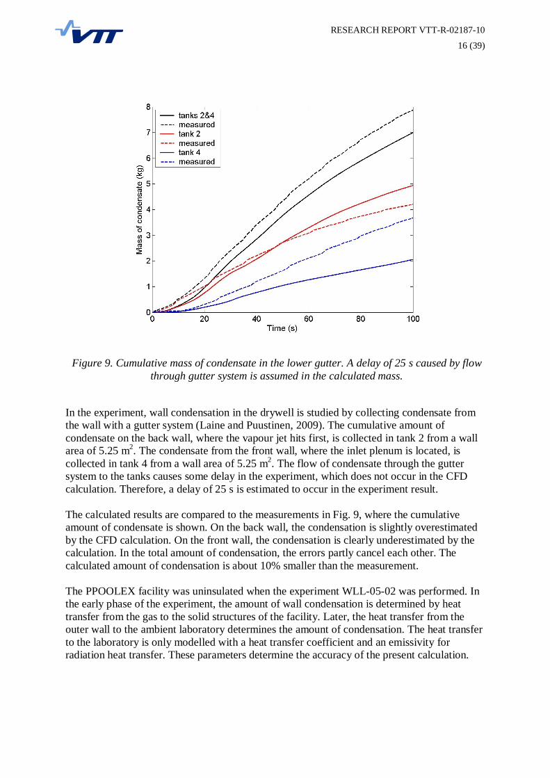
Figure 9. Cumulative mass of condensate in the lower gutter. A delay of 25 s caused by flowthrough gutter system is assumed in the calculated mass.

In the experiment, wall condensation in the drywell is studied by collecting condensate fromthe wall with a gutter system (Laine and Puustinen, 2009). The cumulative amount ofcondensate on the back wall, where the vapour jet hits first, is collected in tank 2 from a wallarea of 5.25 m2. The condensate from the front wall, where the inlet plenum is located, iscollected in tank 4 from a wall area of 5.25 m2. The flow of condensate through the guttersystem to the tanks causes some delay in the experiment, which does not occur in the CFDcalculation. Therefore, a delay of 25 s is estimated to occur in the experiment result.

The calculated results are compared to the measurements in Fig. 9, where the cumulativeamount of condensate is shown. On the back wall, the condensation is slightly overestimatedby the CFD calculation. On the front wall, the condensation is clearly underestimated by thecalculation. In the total amount of condensation, the errors partly cancel each other. Thecalculated amount of condensation is about 10% smaller than the measurement.

The PPOOLEX facility was uninsulated when the experiment WLL0502 was performed. Inthe early phase of the experiment, the amount of wall condensation is determined by heattransfer from the gas to the solid structures of the facility. Later, the heat transfer from theouter wall to the ambient laboratory determines the amount of condensation. The heat transferto the laboratory is only modelled with a heat transfer coefficient and an emissivity forradiation heat transfer. These parameters determine the accuracy of the present calculation.


17 (39)

Figure 10. Comparison of the calculated and measured temperatures in the drywell (top)and in the wetwell (bottom).


18 (39)

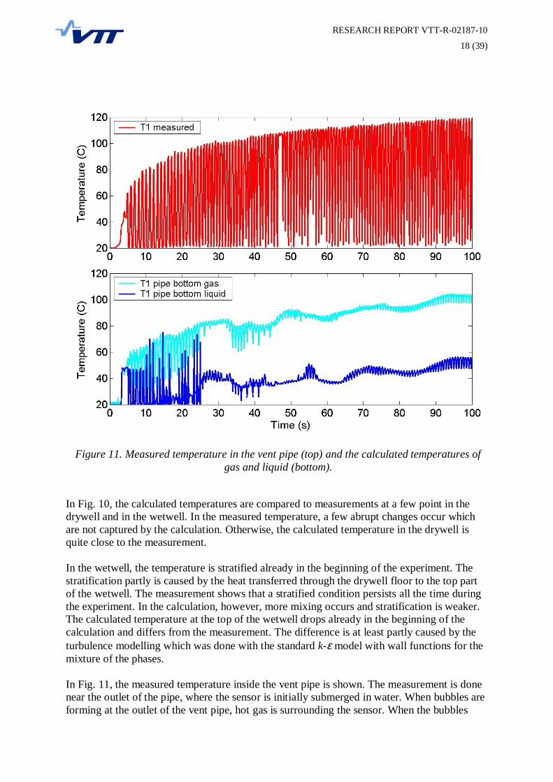
Figure 11. Measured temperature in the vent pipe (top) and the calculated temperatures ofgas and liquid (bottom).

In Fig. 10, the calculated temperatures are compared to measurements at a few point in thedrywell and in the wetwell. In the measured temperature, a few abrupt changes occur whichare not captured by the calculation. Otherwise, the calculated temperature in the drywell isquite close to the measurement.

In the wetwell, the temperature is stratified already in the beginning of the experiment. Thestratification partly is caused by the heat transferred through the drywell floor to the top partof the wetwell. The measurement shows that a stratified condition persists all the time duringthe experiment. In the calculation, however, more mixing occurs and stratification is weaker.The calculated temperature at the top of the wetwell drops already in the beginning of thecalculation and differs from the measurement. The difference is at least partly caused by theturbulence modelling which was done with the standard kε model with wall functions for themixture of the phases.

In Fig. 11, the measured temperature inside the vent pipe is shown. The measurement is donenear the outlet of the pipe, where the sensor is initially submerged in water. When bubbles areforming at the outlet of the vent pipe, hot gas is surrounding the sensor. When the bubbles


19 (39)

detach from the vent outlet, water flows in the vent pipe surrounding the sensor. Therefore,the sensor alternates in measuring the gas and the water temperatures.

In the bottom part of Fig. 11, the calculated temperatures of gas and water are shown. Thecalculated temperatures of gas are somewhat lower than the measurements. The calculatedtemperature of water is higher than the measured value. This indicates that the calculatedmixing of water near the vent outlet is not quite as strong as it is in reality.

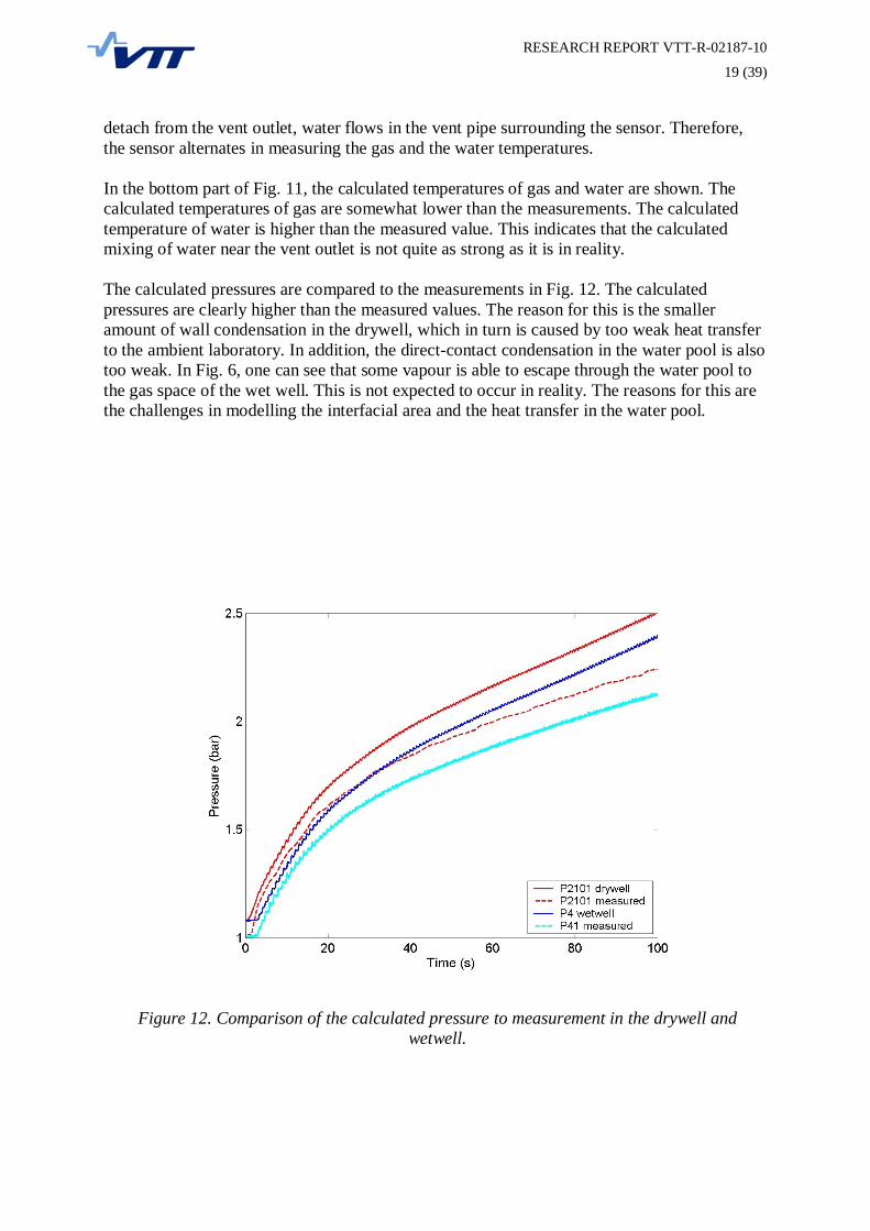
The calculated pressures are compared to the measurements in Fig. 12. The calculatedpressures are clearly higher than the measured values. The reason for this is the smalleramount of wall condensation in the drywell, which in turn is caused by too weak heat transferto the ambient laboratory. In addition, the directcontact condensation in the water pool is alsotoo weak. In Fig. 6, one can see that some vapour is able to escape through the water pool tothe gas space of the wet well. This is not expected to occur in reality. The reasons for this arethe challenges in modelling the interfacial area and the heat transfer in the water pool.

Figure 12. Comparison of the calculated pressure to measurement in the drywell andwetwell.


20 (39)

5 Fluidstructure interaction calculations

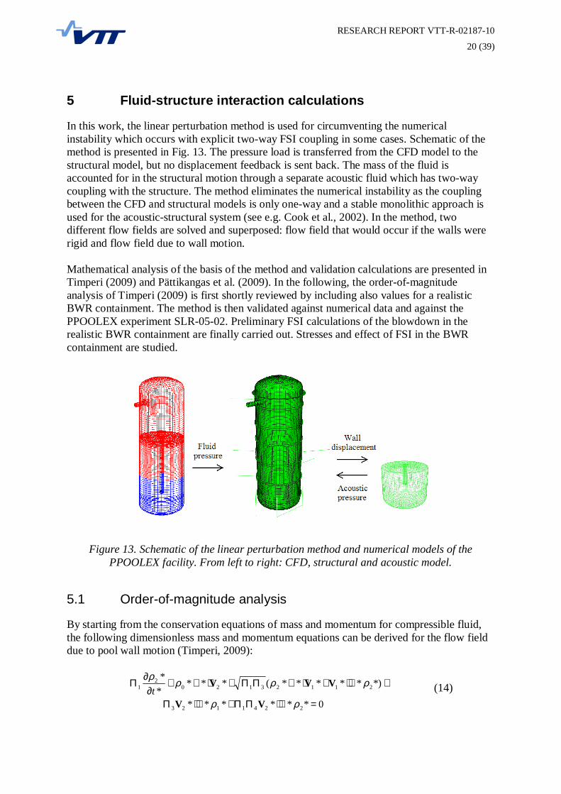
In this work, the linear perturbation method is used for circumventing the numericalinstability which occurs with explicit twoway FSI coupling in some cases. Schematic of themethod is presented in Fig. 13. The pressure load is transferred from the CFD model to thestructural model, but no displacement feedback is sent back. The mass of the fluid isaccounted for in the structural motion through a separate acoustic fluid which has twowaycoupling with the structure. The method eliminates the numerical instability as the couplingbetween the CFD and structural models is only oneway and a stable monolithic approach isused for the acousticstructural system (see e.g. Cook et al., 2002). In the method, twodifferent flow fields are solved and superposed: flow field that would occur if the walls wererigid and flow field due to wall motion.

Mathematical analysis of the basis of the method and validation calculations are presented inTimperi (2009) and Pättikangas et al. (2009). In the following, the orderofmagnitudeanalysis of Timperi (2009) is first shortly reviewed by including also values for a realisticBWR containment. The method is then validated against numerical data and against thePPOOLEX experiment SLR0502. Preliminary FSI calculations of the blowdown in therealistic BWR containment are finally carried out. Stresses and effect of FSI in the BWRcontainment are studied.

Figure 13. Schematic of the linear perturbation method and numerical models of thePPOOLEX facility. From left to right: CFD, structural and acoustic model.

5.1 Orderofmagnitude analysis

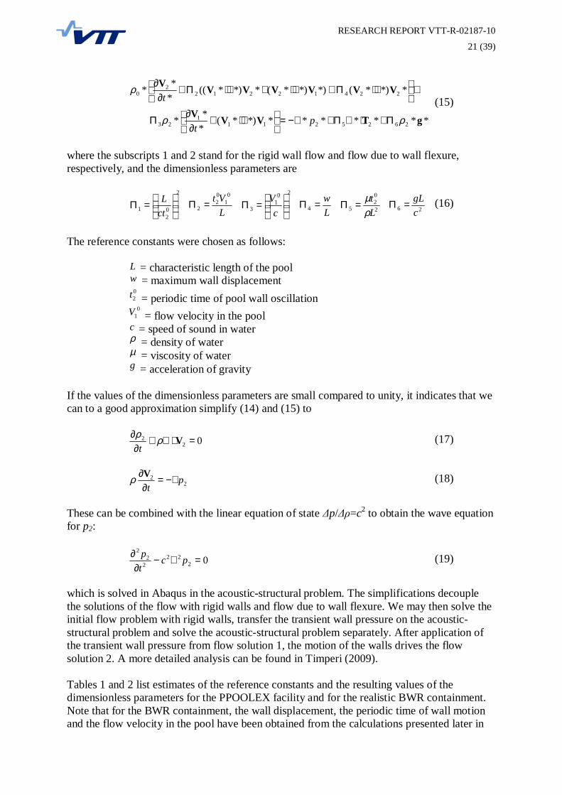
By starting from the conservation equations of mass and momentum for compressible fluid,the following dimensionless mass and momentum equations can be derived for the flow fielddue to pool wall motion (Timperi, 2009):

0******

*)*****(*****

2241123

211231202

1

=⋅∇ΠΠ+⋅∇Π

+⋅∇+⋅∇ΠΠ+⋅∇+∂

∂Π

ρρ

ρρρρ

VV

VVVt (14)


21 (39)

********)*(***

**)*(*)*)*(**)*((***

26252111

23

224122122

0

gTVVV

VVVVVVV

ρρ

ρ

Π+⋅∇Π+−∇=

⋅∇+

∂∂

Π

+

⋅∇Π+⋅∇+⋅∇Π+

∂∂

pt

t (15)

where the subscripts 1 and 2 stand for the rigid wall flow and flow due to wall flexure,respectively, and the dimensionless parameters are

2

02

1

=Π

ctL

LVt 0

102

2 =Π20

13

=Π

cV

Lw

=Π4 2

02

5 Lt

ρµ

=Π 26 cgL

=Π (16)

The reference constants were chosen as follows:

L = characteristic length of the poolw = maximum wall displacement

02t = periodic time of pool wall oscillation

01V = flow velocity in the pool

c = speed of sound in waterρ = density of waterµ = viscosity of waterg = acceleration of gravity

If the values of the dimensionless parameters are small compared to unity, it indicates that wecan to a good approximation simplify (14) and (15) to

022 =⋅∇+

∂∂ Vρρ

t(17)

22 p

t−∇=

∂∂Vρ (18)

These can be combined with the linear equation of state p/ =c2 to obtain the wave equationfor p2:

0222

22

2

=∇−∂

∂ pctp (19)

which is solved in Abaqus in the acousticstructural problem. The simplifications decouplethe solutions of the flow with rigid walls and flow due to wall flexure. We may then solve theinitial flow problem with rigid walls, transfer the transient wall pressure on the acousticstructural problem and solve the acousticstructural problem separately. After application ofthe transient wall pressure from flow solution 1, the motion of the walls drives the flowsolution 2. A more detailed analysis can be found in Timperi (2009).

Tables 1 and 2 list estimates of the reference constants and the resulting values of thedimensionless parameters for the PPOOLEX facility and for the realistic BWR containment.Note that for the BWR containment, the wall displacement, the periodic time of wall motionand the flow velocity in the pool have been obtained from the calculations presented later in


22 (39)

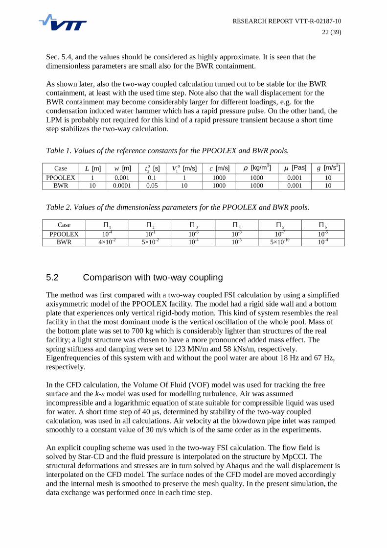
Sec. 5.4, and the values should be considered as highly approximate. It is seen that thedimensionless parameters are small also for the BWR containment.

As shown later, also the twoway coupled calculation turned out to be stable for the BWRcontainment, at least with the used time step. Note also that the wall displacement for theBWR containment may become considerably larger for different loadings, e.g. for thecondensation induced water hammer which has a rapid pressure pulse. On the other hand, theLPM is probably not required for this kind of a rapid pressure transient because a short timestep stabilizes the twoway calculation.

Table 1. Values of the reference constants for the PPOOLEX and BWR pools.

Case L [m] w [m] 02t [s] 0

1V [m/s] c [m/s] ρ [kg/m3] µ [Pas] g [m/s2]PPOOLEX 1 0.001 0.1 1 1000 1000 0.001 10

BWR 10 0.0001 0.05 10 1000 1000 0.001 10

Table 2. Values of the dimensionless parameters for the PPOOLEX and BWR pools.

Case 1Π 2Π 3Π 4Π 5Π 6ΠPPOOLEX 104 101 106 103 107 105

BWR 4×102 5×102 104 105 5×1010 104

5.2 Comparison with twoway coupling

The method was first compared with a twoway coupled FSI calculation by using a simplifiedaxisymmetric model of the PPOOLEX facility. The model had a rigid side wall and a bottomplate that experiences only vertical rigidbody motion. This kind of system resembles the realfacility in that the most dominant mode is the vertical oscillation of the whole pool. Mass ofthe bottom plate was set to 700 kg which is considerably lighter than structures of the realfacility; a light structure was chosen to have a more pronounced added mass effect. Thespring stiffness and damping were set to 123 MN/m and 58 kNs/m, respectively.Eigenfrequencies of this system with and without the pool water are about 18 Hz and 67 Hz,respectively.

In the CFD calculation, the Volume Of Fluid (VOF) model was used for tracking the freesurface and the k model was used for modelling turbulence. Air was assumedincompressible and a logarithmic equation of state suitable for compressible liquid was usedfor water. A short time step of 40 s, determined by stability of the twoway coupledcalculation, was used in all calculations. Air velocity at the blowdown pipe inlet was rampedsmoothly to a constant value of 30 m/s which is of the same order as in the experiments.

An explicit coupling scheme was used in the twoway FSI calculation. The flow field issolved by StarCD and the fluid pressure is interpolated on the structure by MpCCI. Thestructural deformations and stresses are in turn solved by Abaqus and the wall displacement isinterpolated on the CFD model. The surface nodes of the CFD model are moved accordinglyand the internal mesh is smoothed to preserve the mesh quality. In the present simulation, thedata exchange was performed once in each time step.


23 (39)

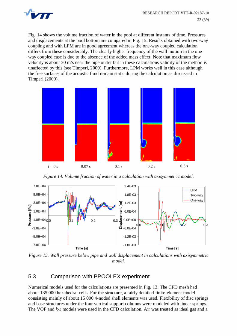
Fig. 14 shows the volume fraction of water in the pool at different instants of time. Pressuresand displacements at the pool bottom are compared in Fig. 15. Results obtained with twowaycoupling and with LPM are in good agreement whereas the oneway coupled calculationdiffers from these considerably. The clearly higher frequency of the wall motion in the oneway coupled case is due to the absence of the added mass effect. Note that maximum flowvelocity is about 30 m/s near the pipe outlet but in these calculations validity of the method isunaffected by this (see Timperi, 2009). Furthermore, LPM works well in this case althoughthe free surfaces of the acoustic fluid remain static during the calculation as discussed inTimperi (2009).

t = 0 s 0.07 s 0.1 s 0.2 s 0.3 s

Figure 14. Volume fraction of water in a calculation with axisymmetric model.

7.0E+04

5.0E+04

3.0E+04

1.0E+04

1.0E+04

3.0E+04

5.0E+04

7.0E+04

0.0 0.1 0.2 0.3

Time [s]

Pres

sure

[Pa]

1.8E03

1.2E03

6.0E04

0.0E+00

6.0E04

1.2E03

1.8E03

2.4E03

0.0 0.1 0.2 0.3

Time [s]

Dis

plac

emen

t [m

]

LPMTwowayOneway

Figure 15. Wall pressure below pipe and wall displacement in calculations with axisymmetricmodel.

5.3 Comparison with PPOOLEX experiment

Numerical models used for the calculations are presented in Fig. 13. The CFD mesh hadabout 135 000 hexahedral cells. For the structure, a fairly detailed finiteelement modelconsisting mainly of about 15 000 4noded shell elements was used. Flexibility of disc springsand base structures under the four vertical support columns were modeled with linear springs.The VOF and k models were used in the CFD calculation. Air was treated as ideal gas and a


24 (39)

logarithmic equation of state was used for water. Mass flow of air at the drywell inlet was setto a constant value of 805 g/s.

These calculations are the same as in Pättikangas et al. (2009) except for some modifications.Firstly, flexibility of the disc springs was adjusted to better fit the measured data. Secondly, aconstant mass flow of air was used instead of the measured mass flow curve. The secondmodification was made because in Pättikangas et al. (2009) charging of the drywell with airwas found to be significantly slower in the calculation compared to the experiment which isprobably caused by delay in the mass flow sensor (Puustinen, 2008). As discussed below, thecharging is still too slow in the calculation. One possible source for this difference is that alsothe measured maximum flow rate of 805 g/s is lower than in reality due to the slow responseof the sensor.

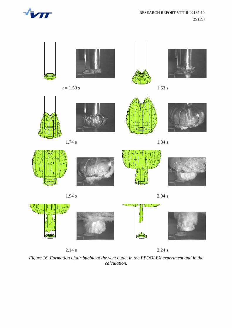
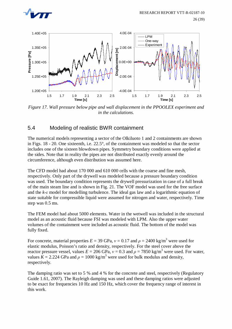
Formation of the first bubble in the pool is shown in Fig. 16 for the calculation andexperiment. Pressures and vertical displacements at the pool bottom are compared in Fig. 17.Charging of the drywell with air is still somewhat slower in the calculation, viz. the firstbubble appears at the pipe outlet at t = 1.9 s and t = 1.5 s in the calculation and experiment,respectively. Therefore, in the figures times between the calculation and experiment havebeen synchronized to the moment when the first bubble appears. It is seen that the calculationwith LPM shows qualitatively correct results. The wall pressure can be in this case separatedinto the components described in Timperi (2009): pressure caused by the blowdown and bywall motion. The calculation with rigid walls shows only the blowdown load, i.e. the effect ofwall motion is not included. Amplitude and frequency of the pool motion obtained with LPMare fairly close to the experiment. The motion is mainly due to vertical oscillation of thewhole pool and its frequency is about 12 Hz. The frequency is about 1.5 times higher in theoneway coupled calculation due to the absence of water. The smaller displacements obtainedwith oneway coupling may be caused by the higher eigenfrequency of the empty pool. Inaddition, damping of the pool motion is faster when the mass of water is neglected.


25 (39)

t = 1.53 s 1.63 s

1.74 s 1.84 s

1.94 s 2.04 s

2.14 s 2.24 s

Figure 16. Formation of air bubble at the vent outlet in the PPOOLEX experiment and in thecalculation.


26 (39)

1.20E+05

1.25E+05

1.30E+05

1.35E+05

1.40E+05

1.5 1.7 1.9 2.1 2.3 2.5Time [s]

Pres

sure

[Pa]

4.0E04

2.0E04

0.0E+00

2.0E04

4.0E04

1.5 1.7 1.9 2.1 2.3 2.5Time [s]

Dis

plac

emen

t [m

]

LPMOnewayExperiment

Figure 17. Wall pressure below pipe and wall displacement in the PPOOLEX experiment andin the calculations.

5.4 Modeling of realistic BWR containment

The numerical models representing a sector of the Olkiluoto 1 and 2 containments are shownin Figs. 18 20. One sixteenth, i.e. 22.5°, of the containment was modeled so that the sectorincludes one of the sixteen blowdown pipes. Symmetry boundary conditions were applied atthe sides. Note that in reality the pipes are not distributed exactly evenly around thecircumference, although even distribution was assumed here.

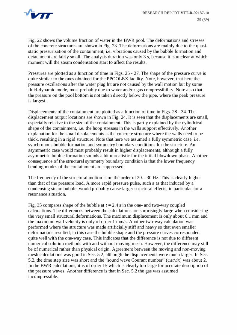
The CFD model had about 170 000 and 610 000 cells with the coarse and fine mesh,respectively. Only part of the drywell was modeled because a pressure boundary conditionwas used. The boundary condition represents the drywell pressurization in case of a full breakof the main steam line and is shown in Fig. 21. The VOF model was used for the free surfaceand the k model for modelling turbulence. The ideal gas law and a logarithmic equation ofstate suitable for compressible liquid were assumed for nitrogen and water, respectively. Timestep was 0.5 ms.

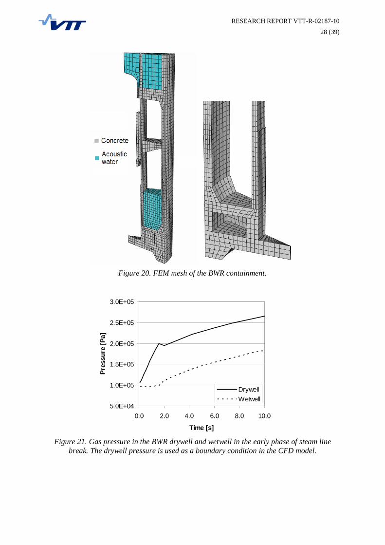
The FEM model had about 5000 elements. Water in the wetwell was included in the structuralmodel as an acoustic fluid because FSI was modeled with LPM. Also the upper watervolumes of the containment were included as acoustic fluid. The bottom of the model wasfully fixed.

For concrete, material properties E = 39 GPa, = 0.17 and = 2400 kg/m3 were used forelastic modulus, Poisson’s ratio and density, respectively. For the steel cover above thereactor pressure vessel, values E = 206 GPa, = 0.3 and = 7850 kg/m3 were used. For water,values K = 2.224 GPa and = 1000 kg/m3 were used for bulk modulus and density,respectively.

The damping ratio was set to 5 % and 4 % for the concrete and steel, respectively (RegulatoryGuide 1.61, 2007). The Rayleigh damping was used and these damping ratios were adjustedto be exact for frequencies 10 Hz and 150 Hz, which cover the frequency range of interest inthis work.


27 (39)

Figure 18. CFD geometry and mesh of the BWR containment.

Figure 19. Refined mesh of the BWR containment near pipe outlet.


28 (39)

Figure 20. FEM mesh of the BWR containment.

5.0E+04

1.0E+05

1.5E+05

2.0E+05

2.5E+05

3.0E+05

0.0 2.0 4.0 6.0 8.0 10.0

Time [s]

Pres

sure

[Pa]

DrywellWetwell

Figure 21. Gas pressure in the BWR drywell and wetwell in the early phase of steam linebreak. The drywell pressure is used as a boundary condition in the CFD model.


29 (39)

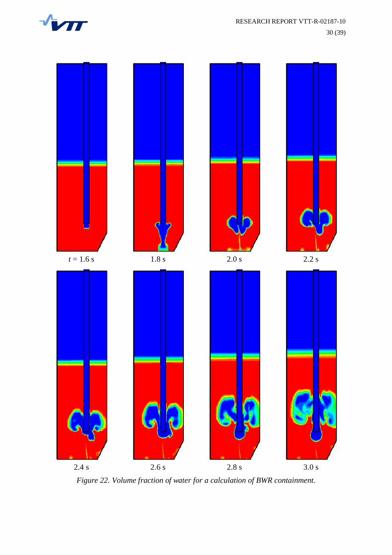
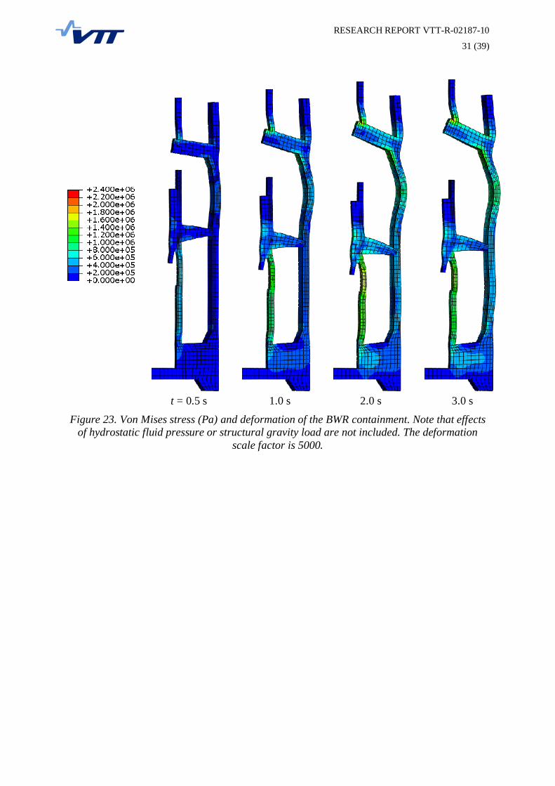
Fig. 22 shows the volume fraction of water in the BWR pool. The deformations and stressesof the concrete structures are shown in Fig. 23. The deformations are mainly due to the quasistatic pressurization of the containment, i.e. vibrations caused by the bubble formation anddetachment are fairly small. The analysis duration was only 3 s, because it is unclear at whichmoment will the steam condensation start to affect the results.

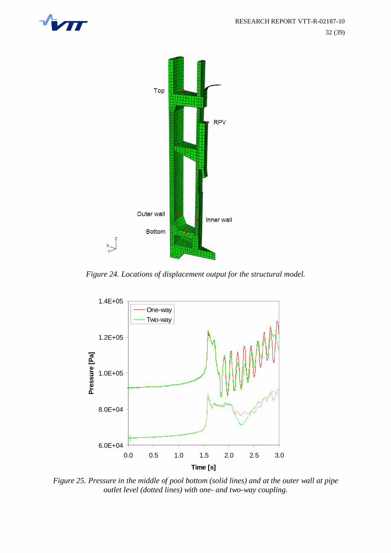
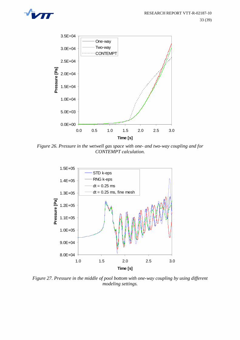
Pressures are plotted as a function of time in Figs. 25 27. The shape of the pressure curve isquite similar to the ones obtained for the PPOOLEX facility. Note, however, that here thepressure oscillations after the water plug hit are not caused by the wall motion but by somefluiddynamic mode, most probably due to water and/or gas compressibility. Note also thatthe pressure on the pool bottom is not taken directly below the pipe, where the peak pressureis largest.

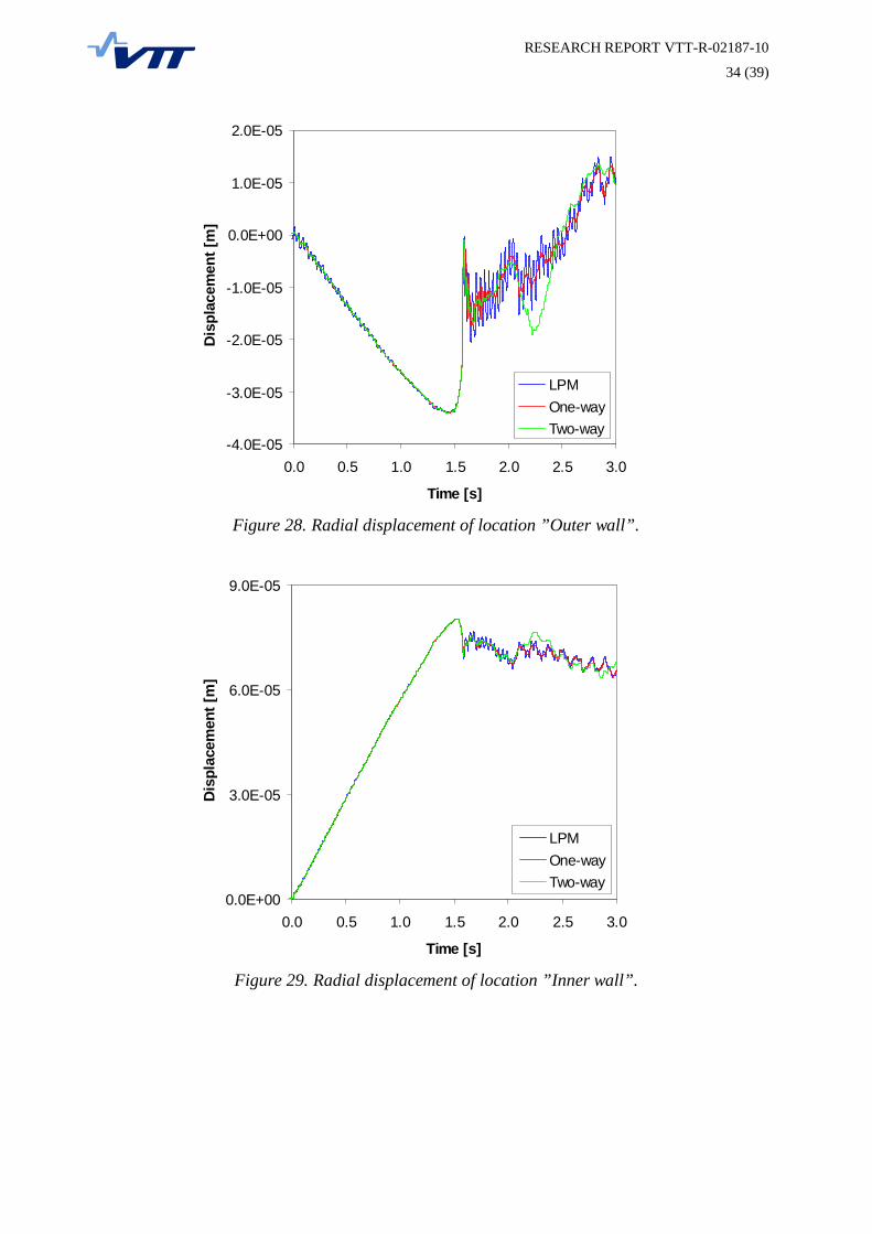
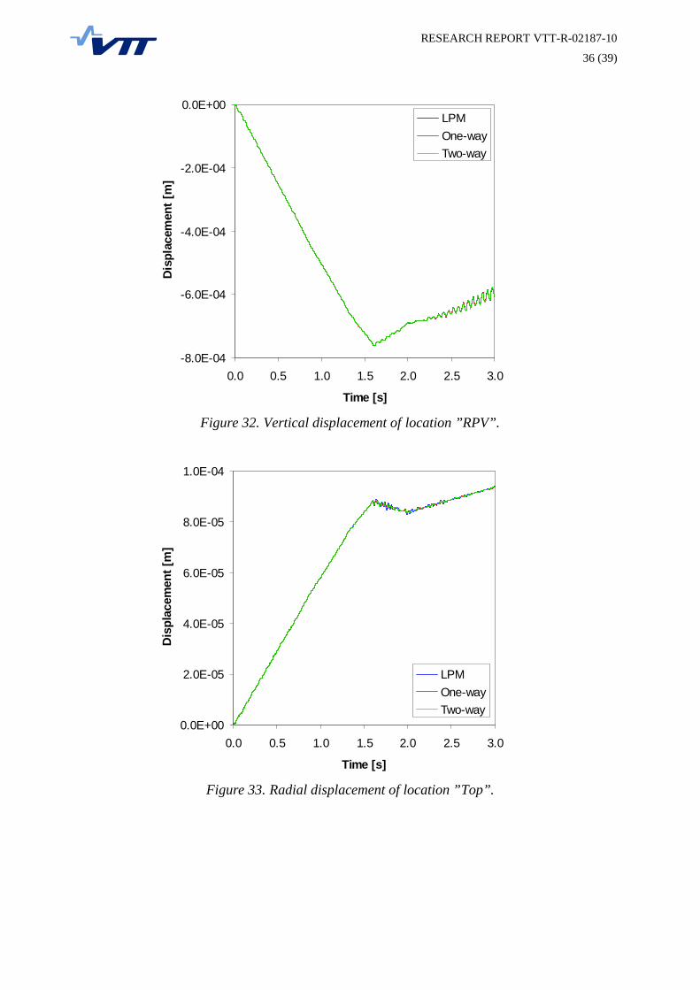
Displacements of the containment are plotted as a function of time in Figs. 28 34. Thedisplacement output locations are shown in Fig. 24. It is seen that the displacements are small,especially relative to the size of the containment. This is partly explained by the cylindricalshape of the containment, i.e. the hoop stresses in the walls support effectively. Anotherexplanation for the small displacements is the concrete structure where the walls need to bethick, resulting in a rigid structure. Note that here we assumed a fully symmetric case, i.e.synchronous bubble formation and symmetry boundary conditions for the structure. Anasymmetric case would most probably result in higher displacements, although a fullyasymmetric bubble formation sounds a bit unrealistic for the initial blowdown phase. Anotherconsequence of the structural symmetry boundary condition is that the lower frequencybending modes of the containment are suppressed.

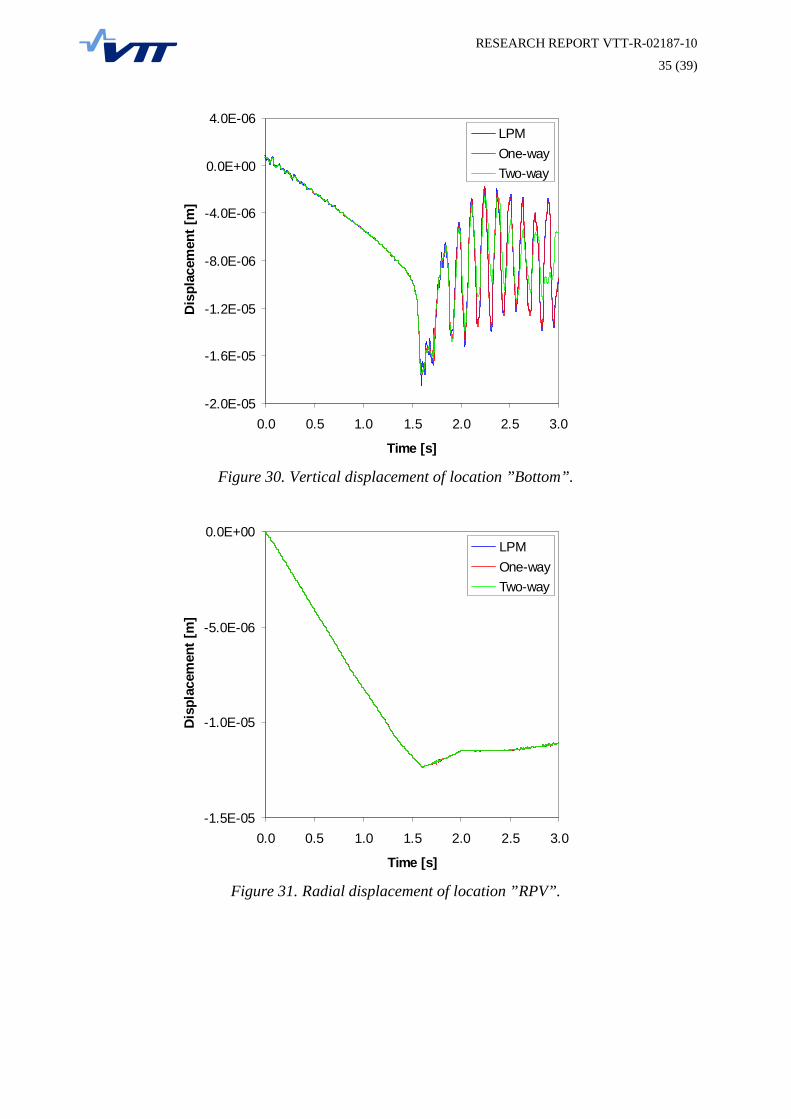
The frequency of the structural motion is on the order of 20… 30 Hz. This is clearly higherthan that of the pressure load. A more rapid pressure pulse, such a as that induced by acondensing steam bubble, would probably cause larger structural effects, in particular for aresonance situation.

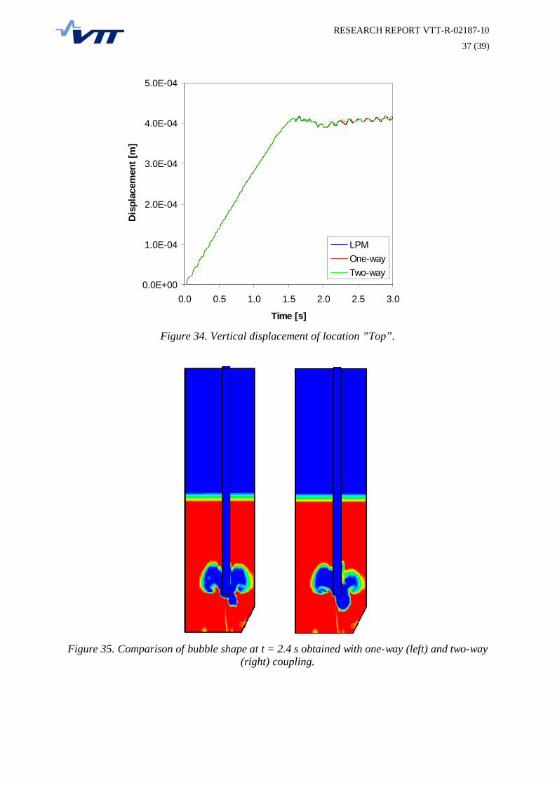
Fig. 35 compares shape of the bubble at t = 2.4 s in the one and twoway coupledcalculations. The differences between the calculations are surprisingly large when consideringthe very small structural deformations. The maximum displacement is only about 0.1 mm andthe maximum wall velocity is only of order 1 mm/s. Another twoway calculation wasperformed where the structure was made artificially stiff and heavy so that even smallerdeformations resulted; in this case the bubble shape and the pressure curves correspondedquite well with the oneway case. This indicates that the difference is not due to differentnumerical solution methods with and without moving mesh. However, the difference may stillbe of numerical rather than physical origin. Agreement between the moving and nonmovingmesh calculations was good in Sec. 5.2, although the displacements were much larger. In Sec.5.2, the time step size was short and the “sound wave Courant number” ( t/ x) was about 2.In the BWR calculations, it is of order 15 which is clearly too large for accurate description ofthe pressure waves. Another difference is that in Sec. 5.2 the gas was assumedincompressible.


30 (39)

t = 1.6 s 1.8 s 2.0 s 2.2 s

2.4 s 2.6 s 2.8 s 3.0 s

Figure 22. Volume fraction of water for a calculation of BWR containment.


31 (39)

t = 0.5 s 1.0 s 2.0 s 3.0 s

Figure 23. Von Mises stress (Pa) and deformation of the BWR containment. Note that effectsof hydrostatic fluid pressure or structural gravity load are not included. The deformation

scale factor is 5000.


32 (39)

Figure 24. Locations of displacement output for the structural model.

6.0E+04

8.0E+04

1.0E+05

1.2E+05

1.4E+05

0.0 0.5 1.0 1.5 2.0 2.5 3.0

Time [s]

Pres

sure

[Pa]

OnewayTwoway

Figure 25. Pressure in the middle of pool bottom (solid lines) and at the outer wall at pipeoutlet level (dotted lines) with one and twoway coupling.


33 (39)

0.0E+00

5.0E+03

1.0E+04

1.5E+04

2.0E+04

2.5E+04

3.0E+04

3.5E+04

0.0 0.5 1.0 1.5 2.0 2.5 3.0

Time [s]

Pres

sure

[Pa]

OnewayTwowayCONTEMPT

Figure 26. Pressure in the wetwell gas space with one and twoway coupling and forCONTEMPT calculation.

8.0E+04

9.0E+04

1.0E+05

1.1E+05

1.2E+05

1.3E+05

1.4E+05

1.5E+05

1.0 1.5 2.0 2.5 3.0

Time [s]

Pres

sure

[Pa]

STD kepsRNG kepsdt = 0.25 msdt = 0.25 ms, fine mesh

Figure 27. Pressure in the middle of pool bottom with oneway coupling by using differentmodeling settings.


34 (39)

4.0E05

3.0E05

2.0E05

1.0E05

0.0E+00

1.0E05

2.0E05

0.0 0.5 1.0 1.5 2.0 2.5 3.0

Time [s]

Dis

plac

emen

t [m

]

LPMOnewayTwoway

Figure 28. Radial displacement of location ”Outer wall”.

0.0E+00

3.0E05

6.0E05

9.0E05

0.0 0.5 1.0 1.5 2.0 2.5 3.0

Time [s]

Dis

plac

emen

t [m

]

LPMOnewayTwoway

Figure 29. Radial displacement of location ”Inner wall”.


35 (39)

2.0E05

1.6E05

1.2E05

8.0E06

4.0E06

0.0E+00

4.0E06

0.0 0.5 1.0 1.5 2.0 2.5 3.0

Time [s]

Dis

plac

emen

t [m

]

LPMOnewayTwoway

Figure 30. Vertical displacement of location ”Bottom”.

1.5E05

1.0E05

5.0E06

0.0E+00

0.0 0.5 1.0 1.5 2.0 2.5 3.0

Time [s]

Dis

plac

emen

t [m

]

LPMOnewayTwoway

Figure 31. Radial displacement of location ”RPV”.


36 (39)

8.0E04

6.0E04

4.0E04

2.0E04

0.0E+00

0.0 0.5 1.0 1.5 2.0 2.5 3.0

Time [s]

Dis

plac

emen

t [m

]

LPMOnewayTwoway

Figure 32. Vertical displacement of location ”RPV”.

0.0E+00

2.0E05

4.0E05

6.0E05

8.0E05

1.0E04

0.0 0.5 1.0 1.5 2.0 2.5 3.0

Time [s]

Dis

plac

emen

t [m

]

LPMOnewayTwoway

Figure 33. Radial displacement of location ”Top”.


37 (39)

0.0E+00

1.0E04

2.0E04

3.0E04

4.0E04

5.0E04

0.0 0.5 1.0 1.5 2.0 2.5 3.0

Time [s]

Dis

plac

emen

t [m

]

LPMOnewayTwoway

Figure 34. Vertical displacement of location ”Top”.

Figure 35. Comparison of bubble shape at t = 2.4 s obtained with oneway (left) and twoway(right) coupling.


38 (39)

6 Summary and conclusions

CFD and FEM modelling of has been performed for experiments performed with thePPOOLEX facility, which is a scaleddown model of a BWR pressure suppressioncontainment. A model for wall condensation and a simple model for directcontactcondensation have been implemented in the commercial FLUENT code. The models havebeen tested against the PPOOLEX experiment WLL0502.

Comparison of the wall condensation model to the experiment was complicated by theuninsulated wall of the drywell of PPOOLEX. When the wall structures have been heated bythe hot vapour, the wall condensation is determined by the heat transfer from the outer wall ofthe drywell to the ambient laboratory. In the CFD model, the chosen heat transfer coefficienton the outer wall determines the amount of condensation. In the calculation, this also affectsto pressure level inside the drywell and wetwell.

In modelling the directcontact condensation, the challenges are in the estimation of theinterfacial surface area and the heat transfer coefficient. The heat transfer and condensation inthe present calculation was found to be too weak. Some vapour was able to escape from thewater pool to the gas space of the wetwell. An additional challenge is presented by modellingthe interfacial drag in the different regions. In the drywell, some mist is formed by the bulkcondensation. In the water pool, at the outlet of the vent pipe a large bubble is formed. Inaddition, small air bubbles are carried away by the flow in the water pool. More work isnecessary to find suitable modelling techniques for these phenomena.

FSI calculations were presented by using a linear perturbation method which circumvents thenumerical instability present in some cases with explicit twoway coupling. The method wasfirst validated against a twoway coupled FSI calculation in a simplified blowdown case. Wallpressure and displacement obtained with LPM and with twoway coupling were in goodagreement, whereas with oneway coupling the absence of the added mass effect was clearlyseen. Validation was also performed against the PPOOLEX SLR0502 experiment where airwas blown into the pool water. A reasonable agreement in wall pressure and displacementwas found between the experiment and LPM calculation. Calculation with oneway couplingshowed qualitatively incorrect results for the wall pressure. In addition, the structuraldisplacements were smaller compared to the experiment and to those obtained with LPM.Because of the added mass effects, using only oneway FSI coupling is not necessarilyconservative in condensation pool simulations.

Preliminary FSI calculations of the noncondensable initial phase of LOCA in a BWRcontainment were also carried out. Effect of FSI was quite small due to the relatively stiff andheavy pool structures. The FSI calculations gave only slightly larger displacements than oneway pressure mapping. Stresses and displacements due to the wetwell blowdown load werefairly small and the largest structural effects were caused by quasistatic pressurization of thecontainment. A symmetric case (simultaneous bubble formation for all pipes) was assumed;fully antisymmetric case would give higher loads but may be unrealistic for the initial phase.A partial explanation for the low structural response is the low frequency of the blowdownload compared to the eigenfrequency of the system. Water hammers due to rapidlycondensing steam bubbles could cause considerably larger deformations, in particular for aresonance situation. In addition, FSI should have a larger effect for more rapid pressuretransients.


39 (39)

References

Cook, R., Malkus, D., Plesha, M. and Witt, R., 2002. Concepts and applications of finiteelement analysis. Wiley & Sons, Inc.

Huber, P.W., Kalumuck, K.M. and Sonin, A.A., 1979. Fluidstructure interactions incontainment systems: smallscale experiments and their analysis via a perturbation method.1st International Seminar on FluidStructure Interaction in LWR Systems, held in conjunctionwith the 5th International Conference on Structural Mechanics in Reactor Technology, Berlin,Germany, August 13 17, 1979.

Lahey, R. T. and Moody, F. J., 1993. The thermal hydraulics of a boiling water nuclearreactor. 2nd Edition, American Nuclear Society.

Laine, J. and Puustinen, M., 2009. PPOOLEX experiments on wall condensation. Researchreport, Lappeenranta University of Technology, Nuclear Safety Research Unit, CONDEX3/2008, 34 p.

Puustinen, M., 2008. Personal communication.

Pättikangas, T., Niemi, J. and Timperi, A., 2009. Modelling of blowdown of steam in thepressurized PPOOLEX facility. VTT Technical Research Centre of Finland, Research ReportVTTR0307309, Espoo, Finland, 52 p.

Regulatory Guide 1.61, 2007. Damping values for seismic design of nuclear power plants.U.S. Nuclear Regulatory Commission.

Sonin, A.A. 1980. Rationale for a linear perturbation method for the flow field induced byfluidstructure interactions. Journal of Applied Mechanics, Vol. 47, P. 725728.

Timperi, A. 2009. Fluidstructure interaction calculations using a linear perturbation method.20th International Conference on Structural Mechanics in Reactor Technology, Espoo,Finland, August 9 14, 2009.

Bibliographic Data Sheet NKS-236 Title CFD and FEM modeling of PPOOLEX experiments

Author(s) Timo Pättikangas, Jarto Niemi and Antti Timperi

Affiliation(s) VTT Technical Research Centre of Finland

ISBN 978-87-7893-308-9

Date January 2011

Project NKS-R / POOL

No. of pages 39

No. of tables 2

No. of illustrations 35

No. of references 9

Abstract Large-break LOCA experiment performed with the PPOOLEX

experimental facility is analysed with CFD calculations. Simulation of the first 100 seconds of the experiment is performed by using the Euler-Euler two-phase model of FLUENT 6.3. In wall condensation, the condensing water forms a film layer on the wall surface, which is modelled by mass transfer from the gas phase to the liquid water phase in the near-wall grid cell. The direct-contact condensation in the wetwell is modelled with simple correlations. The wall condensation and direct-contact condensation models are implemented with user-defined functions in FLUENT. Fluid-Structure Interaction (FSI) calculations of the PPOOLEX experiments and of a realistic BWR containment are also presented. Two-way coupled FSI calculations of the experiments have been numerically unstable with explicit coupling. A linear perturbation method is therefore used for preventing the numerical instability. The method is first validated against numerical data and against the PPOOLEX experiments. Preliminary FSI calculations are then performed for a realistic BWR containment by modeling a sector of the containment and one blowdown pipe. For the BWR containment, one- and two-way coupled calculations as well as calculations with LPM are carried out.

Key words Large-break LOCA, Condensation pool, pressure suppression pool, BWR, CFD, fluid-structure interactions, FSI

Available on request from the NKS Secretariat, P.O.Box 49, DK-4000 Roskilde, Denmark. Phone (+45) 4677 4045, fax (+45) 4677 4046, e-mail [email protected], www.nks.org

Documents

Full text - NKS - Nordic Nuclear Safety Research