FULL STATE FEEDBACK CONTROL OF GALVANOMETER

SCANNING SYSTEM

By

John Keane, B.Eng

A thesis submitted to

Dublin City University

for the degree of

Master of Engineering

School of Electronic Engineering

DUBLIN CITY UNIVERSITY

August 1994

Declaration

I hereby certify that this material, which I now submit for assessment on the programme oTstudy leading to the award of Master of Engineering is entirely my own work and has not been taken from the work of others save and to the extent that such work has been cited and acknowledged within the text of my work

Signed

DateI

I O - C > c b — ¿fLy

Abstract

Voice coil actuators are devices used for moving an inertial load at extremely high accelerations and relocating it within micrometers over a limited range of travel The motion produced may be linear or rotational and the travel times may be in the order of milliseconds or less These actuators have applications in computer disk drives, high speed lens focusing, servo valves and laser scanning tools

In this thesis a digital controller is developed for use in voice coil actuator applications The controller is designed for high accuracy and a fast dynamic response Two design methods are presented both of which are developed, simulated and implemented using a laser-scanner experimental rig

In voice coils based systems, the instantaneous rotor position is normally measured using an electro-mechanical sensor connected to the shaft The elimination of the electo-mechamcal sensor is considered Simulation and experimental results are presented for the laser scanning system operating under normal (with a sensor) and 'sensorless' control

Acknowledgements

I wish to express my sincere gratitude to my supervisors, Dr A Murray and Mr J Dowling who provided much appreciated advice, support and encouragement

Thanks to my fellow postgrads in the Power Electronics Laboratory for their kind support and suggestions

I also wish to thank all the technical staff of the school of Electronic Engineering, especially C Maguire, P Wogan, S Neville and D Condell who provided the necessary equipment and help to complete this research

I would like to thank Power Electronics Ireland Ltd, a division of Fobairt, for their financial assistance and finally to my parents whose encouragement contributed greatly to my further edcuation

CONTENTS

CHAPTER 1 INTRODUCTION 1

CHAPTER 2 SYSTEM DESCRIPTION

2 1 Introduction 42 2 Laser deflectors 42 3 Physical Description of Scanner 62 4 Present Scanning Control Technology 82 5 Intuitive Model 8

2 5 1 Mechanical Model 82 5 2 Electrical Model 9

2 6 Summary 12

CHAPTER 3 CONTROL APPROACH

3 1 Introduction 133 2 Emulation Vs direct digital design 133 3 Transfer function Vs state space techniques 143 4 State space representation of galvanometer scanner 153 5 Full state feedback control 163 6 Control structure with full state feedback control 18

3 6 1 Introduction 183 6 2 Introduction of reference input 193 6 3 Integral control 19

3 7 The state estimator 213 7 1 Justification 213 7 2 The prediction estimator 223 7 3 The current estimator 243 7 4 Combined controller and estimator 25

3 8 Summary 27

CHAPTER 4 SYSTEM IDENTIFICATION

4 1 Introduction 284 2 Experimental modelling/system identification 28

i

4 2 1 Introduction 284 2 2 Model type 294 2 3 The ARX model structure 304 2 4 The ARMAX model structure 31

4 3 Implementing system identification 324 4 Comparison between analytical model and identified model 36 4 5 Transfer function to state space representation 374 6 Summary 38

CHAPTER 5 CONTROLLER DESIGN

5 1 Introduction 395 2 Controller root selection 39

5 2 1 Introduction 395 2 2 The ITAE criterion 405 2 3 Ackermanns formula 415 2 4 LQR optimal control 44

5 3 Sample rate selection 475 3 1 Introduction 475 3 2 Signal smoothness __ 485 3 3 Noise and antialiasing filters 49

5 4 Digital design 505 4 1 Direct digital design 52

5 5 Estimator design 535 5 1 Introduction 535 5 2 Selection of estimator gains 545 5 3 The discrete kalman filter 545 5 4 Selection of Rv and Rw 56

5 6 Sensorless control 595 6 1 Introduction 595 6 2 The sensorless topology 595 6 3 Simulation results 60

5 7 Summary 61

CHAPTER 6 IMPLEMENTATION

6 1 Introduction 626 2 Hardware 62

u

6 2 1 Description 626 2 2 DSP 63

6 2 2 1 Introduction 636 2 2 2 Processor requirements 656 2 2 3 The TMS320C30 666 2 2 4 The TMS320C30 CPU 666 2 2 5 System memory 676 2 2 6 Memory maps 676 2 2 7 Reset/Interrupt/Trap vector maps 676 2 2 8 Peripheral bus map 686 2 2 9 Analogue interface 70

6 2 3 External interfaces 706 2 3 1 Output interfaces 716 2 3 2 Input interface 71

6 3 Software design 726 3 1 Introduction 726 3 2 Software development flow 736 3 3 Numerical conditioning 736 3 4 Software description 746 3 5 Algorithm formulation 77

6 4 System integration 786 4 1 Input/output scaling 786 4 2 Calibration of sensor 79

6 5 Test and evaluation 796 5 1 Introduction 796 5 2 Experimental procedure 796 5 3 Performance using the position sensor 80

6 5 3 1 Test with ITAE design 816 5 3 2 Test with LQR design 81

6 5 4 Performance using the sensorless control approach 856 6 Summary 86

CHAPTER 7 CONCLUSIONS AND RECOMMENDATIONS

7 1 Summary and conclusions 887 2 Recommendations 89

7 2 1 Within the voice coil industry . 897 2 2 For further research 90

in

REFERENCE 91

APPENDIX A

A.1 System identification routines A.2 Transformation procedureA.3 Response with various sample times

APPENDIX B

B.l Input interface circuitry B.2 Output interface circuitry B.3 Current sensing circuitry

schematics

APPENDIX C

Generic C source file listing

IV

CHAPTER 1

INTRODUCTION

With the technological advancements which are being made within the computer industry it is becoming increasingly easier to implement faster and more complex control algorithms giving increased flexibility and improved performance m the real time control of dynamic systems This study examines the application of this 'State of the Art' technology to the control of high speed voice coil actuator applications

As the name suggests, historically the voice coil actuator was used in the construction of loudspeakers It consists of an armature which is suspended in a magnetic field produced by either permanent magnets or electromagnets When a current flows through a conductor suspended in such a magnetic field a force is induced on the conductor causing it to move, the direction of movement depending on the direction of current flow through the conductor Nowadays voice coil actuators are used in many applications and are capable of moving an inertial load at extremely high accelerations and relocating it within micrometers over a limited range of travel The motion produced may be linear or rotational and the travel and settling times may be in the order of milliseconds or less [1-1]

Voice coil actuators are most notably used within the computer industry in high performance peripheral 'disk drive1 memories For example the voice coil based IBM 3380K disk drive moves over a 28mm stroke, and when track following can do so with a statistical deviation of less than one micron (approx one third the width of a human hair), providing accelerations of approximately 490 ms'2 [1-2] These actuators are also used in shaker tables, medical equipment, high-speed lens focusing applications, servo valves, and laser scanning tools In fact it is a laser scanning system which is used as the proto-type application for this study

The laser scanner, or more specifically the galvanometnc scanner1 is a limited rotation servo motor consisting of a voice coil actuator upon which is mounted a mirror This servo is designed to have highly linear torque characteristics over

1 There are many other Laser scanning techniques such as Electrooptic deflectors, Acoustiooptic deflectors and polygonal scanners [1-3]

relatively large scan angles2 These servos are in wide commercial use today in diverse positioning applications such as laser display projection, computer output to microfilm, non-impact printing, space communications and infrared detectors used in military night vision systems.

As was stated earlier, advancements in computer technology allow the implementation of not only faster but more complex digital control strategies This additional computing power allows one to develop more robust control algorithms which can take time-varying parameters into account, model unknown disturbances, include fault detection and correction as well as a host of other capabilities unavailable from their analogue counterparts

The purpose of this thesis is to examine the use of this computing flexibility to identify, model and control the dynamics of voice coil based systems using a galvanometnc scanner as a proto-type application It also assesses how the additional 'intelligence' introduced into the control platform by the micro-processor based controller may be used for alternative control techniques

Thesis Structure

The thesis is divided into seven chapters Chapter 1, the introduction, is given as an overview

Chapter 2 is a general description of a galvanometer scanning system, its physical components and applications A general model is developed which will be refined in following chapters

The 'control approach' is presented in chapter 3, which presents a control methodology based on modem state space control techniques The controller structure is presented as is the development of state estimation techniques

Chapter 4 deals with the topic of system identification which is used to develop an accurate model for a G120D scanner as manufactured by General Scanning Inc, Waterton , MA, USA This discussion continues from the general model presented m chapter 2

2 The scan angle is the portion of scan over which useful work is done, it is usually associated with other criteria (e g velocity linearity) which must be maintained during this penod

2

Chapter 5 discusses the design issues involved, from selecting appropriate closed loop pole locations for the controller through to choosing the micro-processor sampling rate Computer simulation is used extensively in this chapter

In chapter 6 the TMS320C30 PC System board is mtroduced as is its application for high speed scanning systems An overview is presented of the system hardware and the discrete controller designed in chapter 5 is implemented on-line Experimental results taken from the G120D scanner are presented for two types of controller, one which uses a position sensor and the other which uses a 'Sensor-less' control approach as developed m chapter 5

Chapter 7 summarises the overall research and gives recommendations for further work and also details how the results presented may be used in other voice-coil actuator applications especially in the lucrative computer disk-dnve industry

3

CHAPTER 2

SYSTEM DESCRIPTION

2 1 INTRODUCTION

Scanning systems are typically composed of three distinct parts, these are optical, electronic and electro-mechanical An example scanning scheme is presented in fig 2 1 below The optical section is usually Trent end' and includes beam generation, modulation and conditioning The electronic sub-system is concerned with data capture and processing as well as the generation of required position co-ordinates The electro­mechanical aspects involve beam positioning and control, it is this aspect which is considered for this study

The advent of laser beam technology has enabled many technological areas to advance Tlying-spot' scanning technology has been one major area which has benefited significantly from the laser industry, allowing certain scanning applications to expand beyond the laboratory stage to full product development Flying spot scanning systems have been in existence for quite a while, television being the single most popular example of such a system Up until recently most flying spot printers have used cathode ray tubes (CRT's) as the light source However, the main problem with the CRT method is that the resulting electron beam is not very bright

The laser however, has extremely high radiance and a highly confined beam, two very important properties m most scanning applications These properties as well as the increase in cost effectiveness of modulating and deflecting laser beams has revolutionised the non impact printing and image generation industries This has placed a greater interest m the laser industry and has resulted in increased research into the applications of lasers

2 2 LASER DEFLECTORS

Laser deflectors are but one sub-system m the overall scanning scheme, (see fig 2 1) nonetheless it is an area of considerable interest in any scanning system The importance of laser deflection systems is that they deflect light beams instead of electron beams The

4

deflection of light is relatively complex when compared to deflecting electron beams, however it does have the advantage that it is much more stable in the face of outside disturbances For example the CRT based systems must be magnetically shielded to prevent distortion of the incident electron beams

Even with the modem developments many high powered lasers have laser head weights in the order of 3 to 4 kg or more [2-1] One method1 to avoid the mechanical problem of moving such weights at high speed is quite simply to reflect the laser beam off low weight mirrors with weights in the order of grams or less These mirrors have coatings optimised for specific wave lengths and have reflectances of 99% or better [2 2] There are two basic laser beam scanning configurations using this method

1. Polygonal scanners

These scanners have a number of plane mirror surfaces or facets which are parallel to and facing outward from the rotational axis Each facet is equi-distant from the rotational axis The mirror assembly is typically mounted on an electnc motor shaft to produce the rotational motion The significant characteristic of a regular polygonal scanner is that it is used to produce repetitively superimposed, unidirectional straight scans The mam advantages of polygonal scanners are speed, wide scan angles and velocity stability However due to their high inertias they are considered impractical for applications requiring rapid changes in scan velocity or start/stop formats [2 3]

2. Galvanometer scanners

The galvanometnc scanner is a limited rotation servo motor consisting of a voice coil actuator upon which is a mirror is mounted This servo is designed to have highly linear torque characteristics over relatively large scan angles This type of scanner is much slower in terms of scans/sec than the polygonal scanner It does however have greater flexibility in terms of following position profiles and does possess the start/stop capability that the polygonal scanner does not Which scanner one would use is therefore application dependent The galvanometer scanner is considered m this work and is described in greater detail below

1 Many other techniques exist for deflecting laser beams most notably electroopUc and acoustoopUc deflectors Both of these methods are solid state in nature and are discussed more fully in [2 7]

5

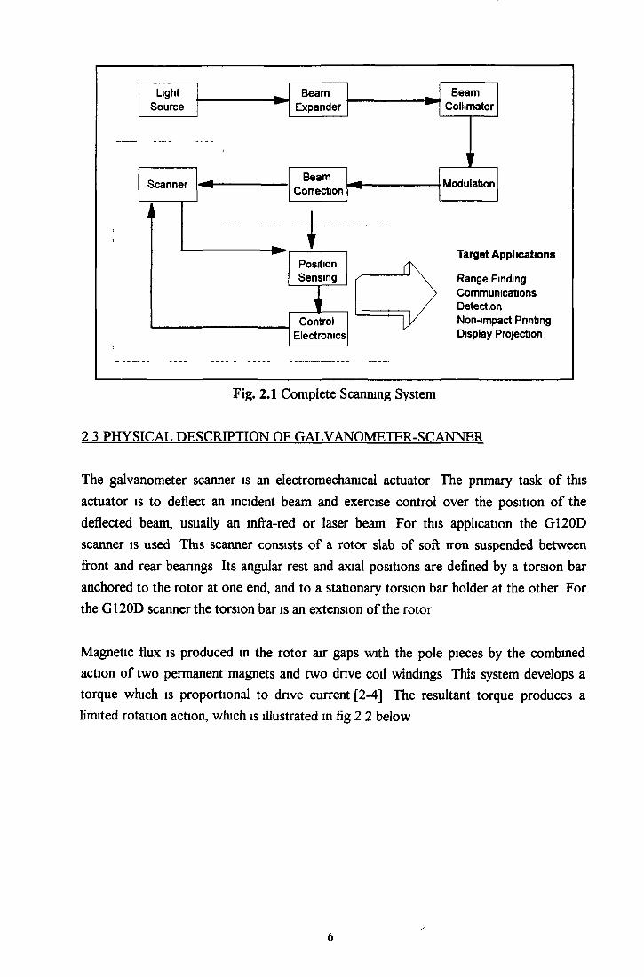
Fig. 2.1 Complete Scanning System

2 3 PHYSICAL DESCRIPTION OF GALVANOMETER-SCANNER

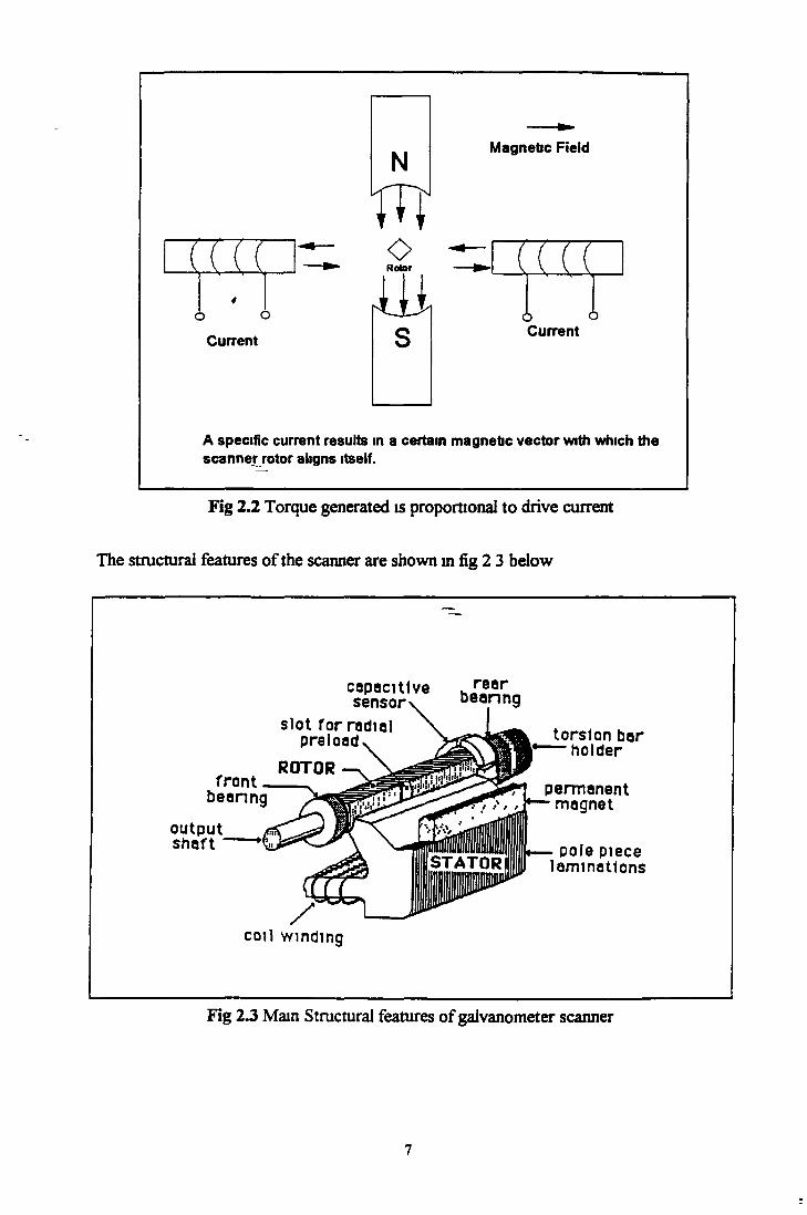
The galvanometer scanner is an electromechanical actuator The primary task of this actuator is to deflect an incident beam and exercise control over the position of the deflected beam, usually an infra-red or laser beam For this application the G120D scanner is used This scanner consists of a rotor slab of soft iron suspended between front and rear bearings Its angular rest and axial positions are defined by a torsion bar anchored to the rotor at one end, and to a stationary torsion bar holder at the other For the G120D scanner the torsion bar is an extension of the rotor

Magnetic flux is produced in the rotor air gaps with the pole pieces by the combined action of two permanent magnets and two drive coil windings This system develops a torque which is proportional to drive current [2-4] The resultant torque produces a limited rotation action, which is illustrated in fig 2 2 below

6

( ( ( (

c

4D C3

Current

N

woRotor

r U J i S

Magnetic Field

nÔ ÒCurrent

A specific current results in a certain magnetic vector with which the scanner^rotor aligns itself.

Fig 2.2 Torque generated is proportional to drive current

The structural features of the scanner are shown in fig 2 3 below

capacitive u,T®arsensorv bearing

front

slot for radial preload.

ROTOR

bearing

outputshaft

torsion bar— holder

permanent- magnet

- pole piece laminations

/coil winding

Fig 2.3 Main Structural features of galvanometer scanner

7

2 4 EXISTING SCANNING CONTROL TECHNOLOGY

For the most part the present controller technology consists of an analogue PID (Proportional, Integral and Derivative) controller While this control approach has been very successful over the past number of years, the advancements made within the computing industry make computer control of mechanical systems more attractive both from a performance as well as economical viewpoint

This work examines the application of digital control techniques to model, identify and control the dynamics of a galvanometer scanner and assesses the advantages or otherwise of these control techniques including their ability to add 'intelligence' to the overall control system

2 5 INTUITIVE MODEL

In order to put these new control techniques into practice, a bridge between the mathematical theory and the real world must be built This bridge is provided by the modelling process and it is this process which is reviewed in this section

In analysing problems in the real world, formulating solutions to these problems or developing theories to explain them, the first step is the development of a mathematical model which adequately describes the system under study A balance must be made between the simplifying assumptions used and the complexity of the model Over simplification may result in an inaccurate model which is not a good representation of the systems actual behaviour while an over complex model may unnecessarily complicate the analysis

Modelling consists of several steps which help to define the goal of the model and discuss it in terms of idealised physical components

2.S.1 Mechanical Model

From section 2 4, the galvanometers mechanical structure can be modelled as in Fig 2 4 below [2 5] The inertia of the rotor, pole pieces and mounted mirror are lumped together in the idealised inertial element J1 , K is the rotor spnng constant and B represents the lumped system damping The rotational equivalent of Newton's equations

1 The system is rotary in nature and hence rotational nomenclature is used

8

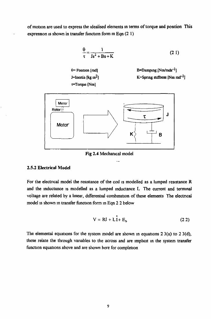
of motion are used to express the idealised elements m terms of torque and position This expression is shown in transfer function form m Eqn (2 1)

6

x1

Js2 +Bs+K(2 1)

0= Position [rad]

J=Inertia [kg m2]

T=Torque [Nm]

B=Damping [Nm/rads-*]

K=Spnng stiffness [Nm rad"̂ ]

2.5.2 Electrical Model

For the electrical model the resistance of the coil is modelled as a lumped resistance R and the inductance is modelled as a lumped inductance L The current and terminal voltage are related by a linear, differential combination of these elements The electrical model is shown m transfer function form in Eqn 2 2 below

V = RI + L I+E k (2 2)

The elemental equations for the system model are shown in equations 2 3(a) to 2 3(d), these relate the through variables to the across and are implicit m the system transfer function equations above and are shown here for completion

9

+K0 = tdt2 dt

x = KtI

(2 3a)

(2 3b)

V = L— +RI +Eb dt b

(2 3c)

E -K dGb b d i

(2 4d)

Eb=Back EMF [V]Kt= Torque constant [Nm A'l]K^=Back EMF constant [Nm A‘l]

The combined mechanical and electrical sub models are obtained on the basis of Fig 2 5 which show the interactions between the two

The block diagram transfer function representation of the system is shown in Fig 2 6 below, this makes more explicit the cause-effect relation that occurs between the two sub models The combined open loop transfer function relating the input voltage V to position 0 may be written as

0 K.

V s3(LJ) + s2(RJ + BL) + s(RJ + KL + KbKt) + KR(2 4)

10

The parameter values used in the above model were obtained from a combination of the manufacturers specifications and measurements taken from the scanner These values are shown m table 1 1 below 1

Table 1.1: Continuous Time Model Parameters

K=0.02 [Nm rad'1]* J=0.028 [kg nt2]*B=1.74*10-6 [Ns-nT1]* Ki=0.005 [Nm A’1]«!»Kb=0.005 [Nm A_1]+ L=0.001 [H]tR=2.3 [Ohms]*

When these values are used in the model of equation (2 4) the following frequency response is obtained which shows the system has an open loop bandwidth of approximately 132 Hz

-20

-60101

• 200

-300101

“ 1--------- 1------ I------1— ! I I") IO n en iooD B ode Dlot

— 1-----T— I f 1 “i----j— j— i— n r* r i

..........................'s .—

102Frequency (rad/sec)

+ i zzr"

102 103Frequency (rad/sec)

104

“ l <----!— I 'l' » )

\

Fig 2.7 Open loop Bode plot

1 * Manufacturers specs, <|> Calculated, t Measured

2 6 SUMMARY

This chapter gave a general overview of flying spot scanning systems and how the galvanometer fits into the family of light deflectors A more detailed description of the galvanometer scanner was then presented as a background for the modelling process The modelling of a dynamic system using a physically intuitive understanding was then outlined and applied to the galvanometer scanning system This modelling process strongly suggests that a third order transfer function description of the system is required to suitably describe the plant This modelling exercise gave an insight into the galvanometer dynamics in that it strongly suggests that a third order model is required to suitably descnbe the plant This information will be used later m chapter 4 on the subject of system identification

12

CHAPTER 3

CONTROL APPROACH

3 1 INTRODUCTION

The topic of'classical control theory' was developed in the penod between the 1930's to the early 1950's This theory was coupled with electronic technology suitable for implementing the required dynamic compensators to give a set of procedures to help solve control problems [3-1]

Since then digital control or sampled-data systems has experienced a surge of interest (and it is within this time that most of this theory was developed) The term 'modem control theory' is used to describe the work which encompasses state space methods as well as optimal and digital control techniques The purpose of this chapter is to examine the types of control strategies which are available for use with this digital control platform and to choose a controller structure which will be fully developed and implemented in later chapters

3 2 EMULATION Vs DIRECT DIGITAL DESIGN

The classical design techniques were based on a transfer function, laplace transform representation of the dynamic system The design is inherently earned out in continuous time using the Bode or root locus techniques The method of indirectly constructing a digital controller from a continuous design is known as emulation or s- plane design The benefits of this approach is that the design is performed in continuous time, the fact that the controller is being implemented on a computer only results in one additional step which is to emulate the resultant controller in discrete form Specifications for most designs are expressed in terms of rise times, settling times, and overshoot These parameters are easily reconciled to continuous time closed loop root locations

The direct digital design method consists of the discretisation of the system model and then to perform the design entirely in the discrete time z-domain With some modifications the classical transform techniques described above are applicable to

13

discrete design The root locus method is transferred unaltered but the results are interpreted in a different manner than in the continuous s-plane The Bode method may also be applied but the transform to the discrete domain is not straight forward and for high order systems may become unwieldy In many situations it is advantageous to use both emulation and direct digital design methods This involves initially determining the discrete controller from the continuous time s-domain using the emulation method, the direct digital method is then used to verify or modify the design before a final controller is chosen The process of this design is covered in more detail m chapter 5 and involves extensive computer simulation

3 3 TRANSFER FUNCTION Vs STATE SPACE TECHNIQUES

The transfer function of a linear time invariant system is defined to be the ratio of the laplace transform of the output variable to the laplace transform of the mput variable in the assumption that all initial conditions are zero[3-2] This input-output relationship is synonymous with the older continuous classical design methods although it can be easily applied to the discrete case Although the transfer function model approach provides simple and powerful analysis design tools it does suffer from a number of short comings

1. A transfer function model is only defined under zero initial conditions

2. It is applicable to linear time invariant systems and becomes highly cumbersome for multi-input multi-output (MIMO) systems

3. It only provides information for a given input and contains no information regarding the internal states of the system This may not suffice in situations where the mput and output of a system are within allowed bounds and yet some of the internal system elements may have exceeded their specified ratings

4. In many situations it is advantageous to feed back some of the internal states of a system rather than just the output This may have the effect of both stabilising and improving system performance

5. The classical design methods such as Bode and root locus are based on iterative tnal and error steps These procedures become unwieldy and difficult to organise for even moderately complex systems

14

6. Having access to all the internal states of the system may have additional benefits resulting m a simplification or reduction of hardware and/or allowing more advanced control

The state space technique represents the system in three types of variable the input, the output variables and the internal or state variables This method enforces the concept that any dynamic system, no matter how complex, may be presented in terms of first order sub models This is in contrast with classical control theory where attention is given to the system characteristic equation which may be of a very high order As well as a reduction m complexity this representation provides a more compact and intuitive model of the plant The state space technique provides a powerful tool for the analysis and design of linear and non-linear, time -invariant or time varying multi-input and multi-output systems The availability of the internal states has some beneficial consequences for the designer especially in relation to points 3-6 above

Although state-space methods have many useful properties, they cannot completely replace the transfer function approach The advantages of using transfer function representation are that the designs are made robust easier and experimental frequency-response data can be used to close a loop quickly without a time consuming modelling effort It is usually used in the preliminary design stage where a complex system is reduced to a more manageable model Nevertheless the state space design method is a powerful tool and is particularly suited for this study in relation to point 6 above

3 4 STATE SPACE REPRESENTATION OF GALVANOMETER SCANNER

The transfer function, derived from physical properties of the system in section 2 5 is now transferred to a state space format This involves combining the equations for the state evolution (2 3a to 2 3d) and the output to give a matrix representation of the open loop transfer function Another benefit of state space design is that this format is suitable for computer manipulation which is reflected in the fact that it is used extensively m CAD tools

15

The generic state space representation is

x(t) = Ax(t) + Bu(t) ^

y(t) = Cx(t)for continuous time and

x(k + l) = Ax(k) + Bu(k) y(k) = Cx(k) '

for discrete time where x(t) and x(k+l) are the continuous and discrete state vectors respectively, u and u(k) the continuous and discrete input vectors Similarly,A is the plant matrix, B is the input coupling matrix, and C is the output coupling matrix As can be seen from (3 1) and (3 2) these matrices are different for the contmuous and discrete cases, i e whether one is discussing x(t) or x(k)

For this application the rotor position, and velocity and coil current are chosen as the states of interest1 The input state is chosen as voltage and the output state as position The continuous state space representation for this system is shown in equations (3 3 a) and (3 3 b) below

0 0 1 0 0 0••0 = -K /J -B /J Kt /J

•0 + 0

•I 0 -K b/L -R /L I 1/L

(3 3a)

0y = |l 0 o|e

(3 3b)

3 5 FULL STATE FEEDBACK CONTROL

The state-space representation is as in equations (3 3a) and (3 3b) above With this representation and assuming all states are available (by measurement or otherwise) to the designer then in this situation full state feedback control can be applied As the

1 The reason for choosing current as a state is discussed in chapter 5

16

name suggests full state feedback control is where all the system states are fed back to the input to influence the location of closed loop poles. The location of these poles has a direct correspondence with the dynamic properties of the system such as rise times, settling times and overshoot. As well as the intrinsic advantages of using all pertinent knowledge about the system as outlined in section 3.3 full state feedback control has the advantage that several optimal control CAD techniques take this form. These are discussed in chapter 5.

The usual feedback scheme is to feedback a linear combination of the states which results in the control input2

u = -K X = -[k jk 2...k n] (3.4)

Where,u = input K = feedback gain matrix X = state vector n=system order

To illustrate how this feedback term can modify the dynamic characteristics of the plant, equation (3.4) is substituted into equation (3.1) to yield

x(t) = Ax(t) - BKx(t) (3.5)

the Laplace-transform for this system is

(si - A + BK)x(t) = 0 (3.6)

which has the following characteristic equation

detjsl - A + BK| = 0 (3.7)

Here we see that the feedback gain matrix K couples directly into the characteristic equation, the roots of which give the closed loop pole locations. In fact this is one of the important properties of full state feedback: unlike classical design, where the parameters in the controller (compensator) are iterated upon in an attempt to come

2 This is for the non-reference input case, the reference input structure is discussed later.

17

up with satisfactory root locations, the full state feedback approach allows us to arbitrarily place the roots in any specified location Thus the full state feedback method guarantees us success if n roots are specified for an order system

The process of finding the gain matrix K given a set of desired root locations is known as pole placement and basically consists of comparing the co-efficients of the desired closed loop characteristic equation to the open loop uncompensated characteristic equation Most control CAD packages contain routmes to calculate the controller feedback gains given a set of desired pole locations These routmes are based on derivatives of the well known Ackermann's formula [3-4 & 3-5]

(

The real design task however, is to find the closed loop root locations which correspond to a set of system specifications or are chosen in an 'optimal sense' As stated above the full state feedback method is suitable for use in an 'optimal control' framework This uses a number of CAD tools which specify a candidate root location set subject to the minimisation of certain cost functions, these cost functions are usually based on control effort, system error or a combination of both These optimal control functions are presented m chapter 5 in the detailed discrete controller design

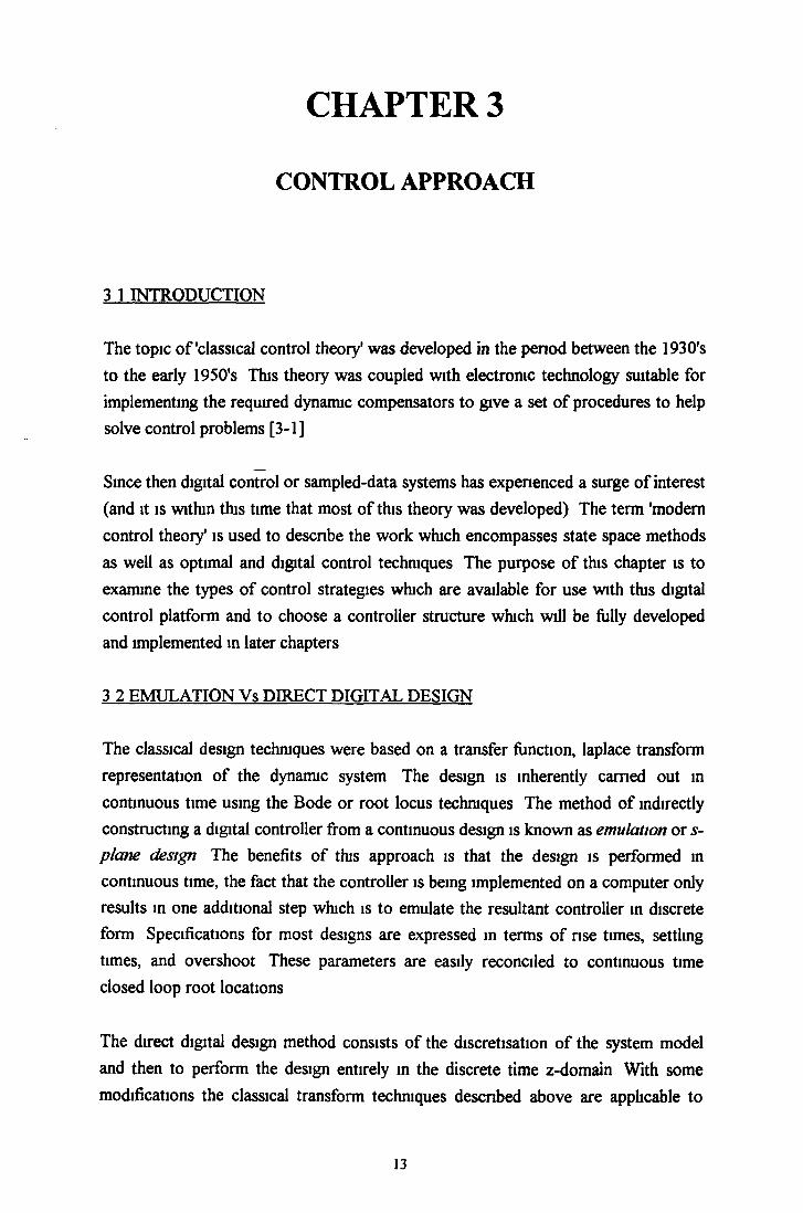
3 6 CONTROLLER STRUCTURE WITH FULL STATE FEEDBACK CONTROL

3.6.1 Introduction

The structure using full state feedback in the control law given by equation (3 4) and shown in fig 3 1 below is for a regulator design The purpose of this design is to bring all the states of the system to zero The galvanometer, whose states are position, current and velocity, clearly necessitates a different type of controller This controller must provide the necessary input to deflect the incident beam through a desired reference angle 0ref This involves the introduction of a reference input into the general regulator structure shown in fig 3 1

18

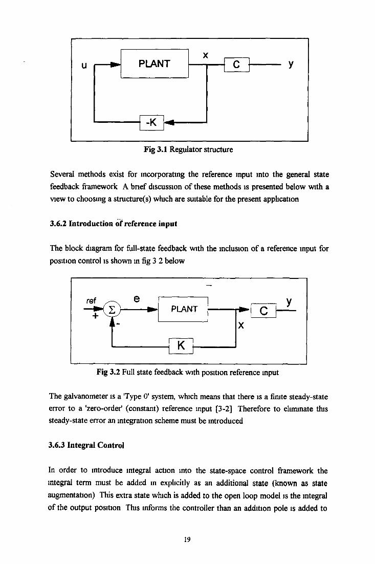
Fig 3.1 Regulator structure

Several methods exist for incorporating the reference input into the general state feedback framework A brief discussion of these methods is presented below with a view to choosing a structured) which are suitable for the present application

3.6.2 Introduction of reference input

The block diagram for full-state feedback with the inclusion of a reference input for position control is shown in fig 3 2 below

Fig 3.2 Full state feedback with position reference input

The galvanometer is a 'Type O' system, which means that there is a finite steady-state error to a 'zero-order' (constant) reference input [3-2] Therefore to eliminate this steady-state error an integration scheme must be introduced

3.6.3 Integral Control

In order to introduce integral action into the state-space control framework the integral term must be added in explicitly as an additional state (known as state augmentation) This extra state which is added to the open loop model is the integral of the output position This informs the controller than an addition pole is added to

19

the system model and that an extra feedback gam must be calculated for this additional state 1 e the augmented model is used in the selection of the controller gains The open loop output integral state is given as

T Tx, = j 0 dt = \ Cx dt (3 8a)

o o

and

(3 8b)

The position integrator does not exist physically on the plant and it must be included externally In the controller closed loop feedback case the output is compared to the reference input before the integration is performed on the resultant error The closed loop integrator output is given as

where Kj is the integrator gam

This results in the integral control with full state feedback structure which is shown m fig 3 4 below As required, the above structure results in a controller which can provide a zero steady state error to a step reference input As can be seen from the continuous transfer function equivalent of a full state feedback system Eqn (3 9), more control is obtained over the positioning of the closed loop poles since the feedback gams couple into all the system modes A more detailed design of this system is presented in chapter 5

Integrator output = jK, *(0ref -y)dt (3 8c)o

20

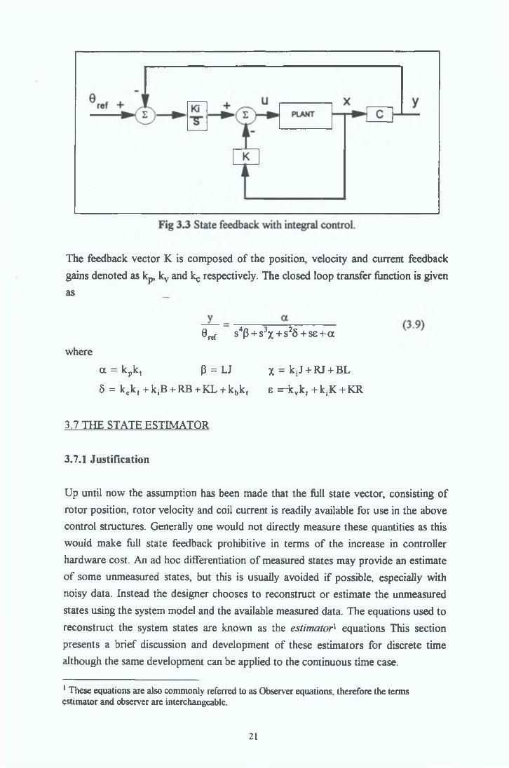
The feedback vector K is composed of the position, velocity and current feedback gains denoted as kp, kv and 1^ respectively. The closed loop transfer function is given as

0ref s4(3 + s3x + s25 + se+oc

where

a = k pk t P = LJ x = kjJ + RJ + BL

5 = kck t +kiB + RB+KL + kbk t 8 ="kvkt + kjK +KR

3.7 THE STATE ESTIMATOR

3.7.1 Justification

Up until now the assumption has been made that the full state vector, consisting of rotor position, rotor velocity and coil current is readily available for use in the above control structures. Generally one would not directly measure these quantities as this would make full state feedback prohibitive in terms of the increase in controller hardware cost. An ad hoc differentiation of measured states may provide an estimate of some unmeasured states, but this is usually avoided if possible, especially with noisy data. Instead the designer chooses to reconstruct or estimate the unmeasured states using the system model and the available measured data. The equations used to reconstruct the system states are known as the estimator1 equations This section presents a brief discussion and development of these estimators for discrete time although the same development can be applied to the continuous time case.

1 These equations are also commonly referred to as Observer equations, therefore the terms estimator and observer are interchangeable.

21

3.7.2 The Prediction Estimator

Under ideal circumstances the system model provides a true representation of the plant dynamics In this case, if the same input is applied to both plant and model the model would reflect the actual plants dynamics and produce the required state vector This is equivalent to operating the estimator in open loop The estimated state vector m this case is therefore given as2

x(k + l) = Ax + Bu(k) (3 10)

The resulting state estimation error is defined as

x = x - x (3 11)

By combimng equation (3 1) and (3 10) the error dynamics of this system are given as

x = Ax (3 12)

The open loop plant dynamics therefore determines the estimator error dynamics For a marginally stable or unstable system the estimator error never decreases to zero For an asymptotically stable system the error will eventually go to zero, but only at the same rate as the system states approach zero

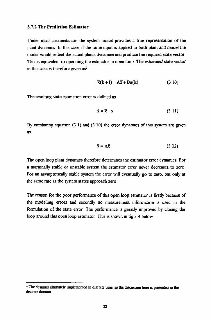
The reason for the poor performance of this open loop estimator is firstly because of the modelling errors and secondly no measurement information is used in the formulation of the state error The performance is greatly improved by closing the loop around this open loop estimator This is shown in fig 3 4 below

2 The desigms ulumately implemented in discrete Ume. so the discussion here is presented in the discrete domain

22

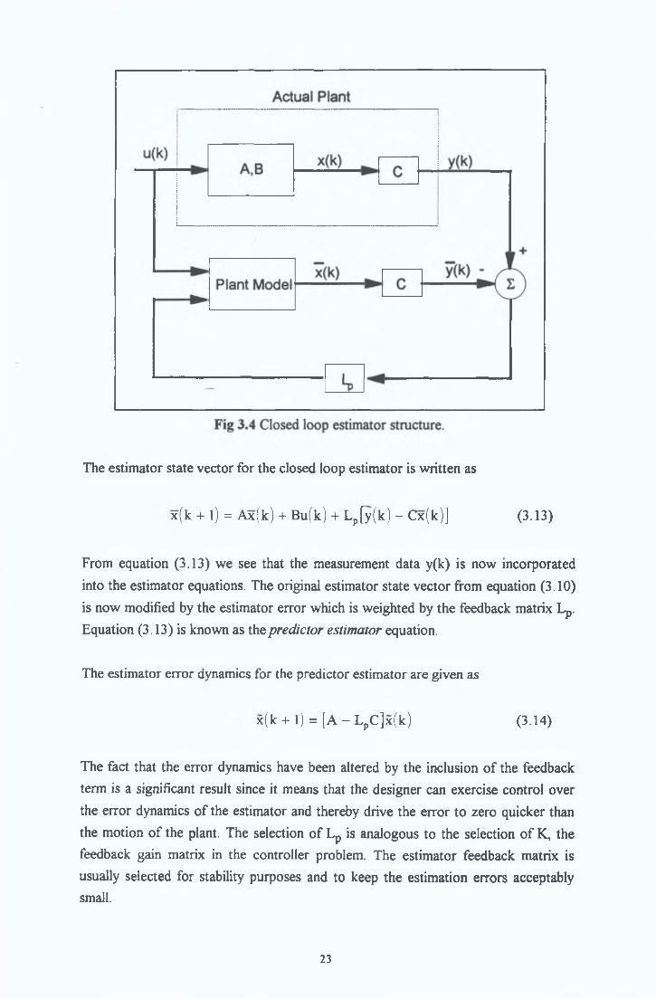
The estimator state vector for the closed loop estimator is written as

x(k + l) = Ax(k) + Bu(k) + Lp[y(k) - Cx(k)] (3.13)

From equation (3.13) we see that the measurement data y(k) is now incorporated into the estimator equations. The original estimator state vector from equation (3.10) is now modified by the estimator error which is weighted by the feedback matrix Lp. Equation (3.13) is known as the predictor estimator equation.

The estimator error dynamics for the predictor estimator are given as

x(k + l) = [ A - L pC]x(k) (3.14)

The fact that the error dynamics have been altered by the inclusion of the feedback term is a significant result since it means that the designer can exercise control over the error dynamics of the estimator and thereby drive the error to zero quicker than the motion of the plant. The selection of Lp is analogous to the selection of K, the feedback gain matrix in the controller problem. The estimator feedback matrix is usually selected for stability purposes and to keep the estimation errors acceptably small.

23

3.7.3 The Current Estimator

As its name suggests the predictor estimator predicts the state vector a sample penod ahead of the measurement (Equation 3 13), this means that the estimated state vector at time k+1 is based on the output measurement taken at time k Since the control equations are in turn based on the estimated state vector, the applied control does not depend on the most recent output measurement This introduced delay is eliminated by using the current estimator.

The current estimator is formulated in such a way that the current estimate x(k) is based on the current measurement y(k) The current estimator equations are shown below

x(k) = x(k) + L(y(k) - Cx(k)) (3 15a)

Where x(k) is the prediction estimate based on the previous estimate at time k-1

x(k) = Ax(k-1) + Bu(k-1) (3 15b)

Using the current estimator the applied control will now depend on the most recent measurement For comparison purposes equation (3 15a) is now substituted into (3 15b) resulting in the predictor estimator of

x(k + l) = Ax(k) + Bu(k) + AL[y(k) - Cx(k)] (3 16)

this equation is similar to the original predictor equation of (3 13) The estimator error equations are found by subtracting equation (3 2) from equation (3 16) which results m

x(k + l) = [A - ALC]x(k) (3 17)

By comparing the above current and predictor estimator equations, it is seen that x in the current estimator is the same quantity as x in the predictor estimator It is also apparent that the estimator gam quantities are related by

Lp = AL (3 18)

24

Therefore either form may be used to calculate the feedback matrix L. As was stated previously the calculation of L in the current equation is very similar to the calculation of the feedback matrix K in the control problem. With some small adjustments Ackermann's pole placement equations may be used directly to calculate Lp and hence L. The current estimator structure, illustrating the relationship between the current and predictor estimators is shown in fig 3.5

In actual implementations the current estimatoHs almost universally chosen as the best estimator structure. Intuitively we would expect it to give a better estimate since it utilises the most recent measurement. Using the latest measurement gives the fastest response to unknown disturbances or measurement noise. The draw back of the current estimate is that it assumes that the controller equations can be executed in zero time. This is clearly not the case resulting in the fact that the control output is slightly 'out of date1 before the equations are completed. This latency is not present in the predictor case since a sample period is available to perform the calculations. Any deficiencies introduced into the current estimator because of this latency can be accounted for by modelling the latency or by further iterations in the desired root locations. In the present application due to the high sampling and processor speeds no significant latency occured and hence the current estimator structure was chosen for the reasons as outlined above.

3.7.4 The Combined Controller and Estimator

The controller design discussed in section 3.6 assumed that all the states are measured directly and then fedback. The Separation Principle Theorem [3-5] tells us that the roots of the complete system consisting of the control law and the estimator

25

will have the same roots as the two cases analysed separately. Therefore the overall system has the following characteristic equation

d e t|z l-A +A LC |det|zI-A + BK| = 0 (3.19)

Error dynamics Control dynamics

As can be seen from equation (3.19) the overall system closed loop roots are comprised of the individual controller and estimator roots combined. Unlike choosing the control root locations where considerations such as actuator size, cost and limitations must be taken into account, choosing the estimator gains does not cost anything in terms of actuator hardware since the estimation process is carried out entirely in software. However, there is an upper limit to the speed of response of the estimator in terms of stability and sensor noise rejection. These considerations are formally formulated in Kalman Filtering Theory which is discussed in chapter 5. In most applications a rule of thumb is to choose roots 2 to 6 times faster than the control roots[3-6]. This is done so that the system response will be dominated by the controller roots, which are in turn derived from the original system specifications.

3.8 SUMMARY

The aim of this chapter is to introduce some of the choice available to the designer and to justify the decisions taken in later chapters. It presents an overview of the modem state-space design techniques. The advantages of the state-space approach

26

over its transfer function equivalent were outlined but it was noted that the state- space approach cannot completely replace its transfer function counterpart

Having decided on a state-space design methodology a number of control structures were examined It was decided to implement the integral control structure usmg the output error topology

The concept of the state estimator, which eliminates the need for additional sensors when usmg the full state feedback is used is also discussed The detailed design of the controller and estimator is presented in chapter S

27

CHAPTER 4

SYSTEM IDENTIFICATION

4 1 INTRODUCTION

The analytical1 system model, which is based on a physical, intuitive understanding of the system and the application of basic physical laws was presented in chapter 2 This model is suitable for the preliminary controller structure selection as earned out m chapter 3 To proceed with a detailed design the system model must be compared closely with the actual plant behaviour The importance of a good model is further emphasised with introduction of estimators and how the system model as well as the measured state is used to reconstruct additional unmeasured states

In this chapter we look at structured methods for formulating system models from measured input-output data This type of modelling has developed into an area known as system identification and it is this topic which is under review m this chapter

4 2 EXPERIMENTAL MODELLING / SYSTEM IDENTIFICATION

4.2.1 Introduction

The analytical method discussed above uses a physical understanding of the system to charactense its dynamic behaviour System identification on the other hand refers to the denvation of mathematical models of dynamic systems from observed data [4-1] This denvation process consists of three parts

1 The input-output data collected dunng some specified identification expenment The user specifies which signals are measured, these are chosen dunng the expenment design to be maximally informative

2 The set of model candidates within which we are going to look for a suitable one This part of the identification procedure depends on a combination of a pnon knowledge and formal properties of models The identification procedure benefits

1 The terms analytical and physical modelling can be used interchangeably

28

here by any insight gained during the analytical modelling stage in chapter 2 giving the user a better understanding of the most suitable model structure

3 Selection of the "best" model from the set of model candidates subject to the observed data The assessment is usually based on how the model can reproduce the observed output data from the observed input data

Although a model can never be accepted as a complete and true description of the system it can be regarded as a good enough description for our intended purposes [4-2]

4.2.2 Model Type

From a prior knowledge of the system a linear time-invanant model set is chosen for this application A discrete linear time invariant model is described by

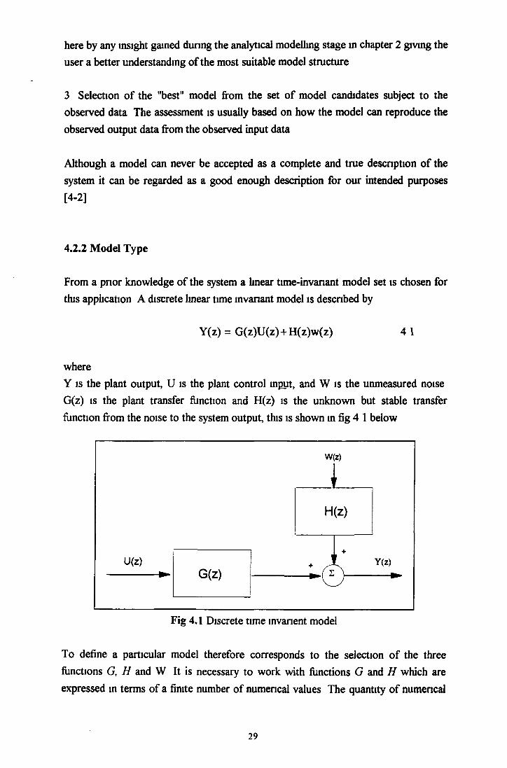
Y(z) = G(z)U(z)+H(z)w(z) 4 1

whereY is the plant output, U is the plant control input, and W is the unmeasured noise G(z) is the plant transfer function and H(z) is the unknown but stable transfer function from the noise to the system output, this is shown in fig 4 1 below

To define a particular model therefore corresponds to the selection of the three functions G, H and W It is necessary to work with functions G and H which are expressed in terms of a finite number of numerical values The quantity of numerical

29

values used determines the order of the model and the way in which these values are calculated and combined determines the model structure The identification process now becomes a search for the best set of parameters 0 which are used in a particular structure or

The estimation procedure is used to select the parameter vector 0 This is usually done by minimising certain error cntena

4.2.3 The ARX model structure

The ARX (Auto-regressive with exogenous input) model is one of the simplest input- output transfer function model types [4-3] It is a linear difference equation which expresses the present output in terms of past inputs and outputs so that

As can be seen from (4 3) the noise enters the model as a direct error in the difference equation and it is therefore often referred to as an equation error structure For this model structure the adjustable parameter vector is

y(z) = G(z,0)u(z)+H(z,0)w(z) (4 2)

y(t) + a,y(t - l)+ +a„ay(t-na)(4 3)

= bju(t-l)+ +b„bu(t-nb) + w(t)

® = [»1 a 2 a„a b, b2 bnJ T (4 4)

in system identification literature it is common to introduce

A(z *) = l + a,z * + +a„az "a (4 5)

and

B(z-t) = bjZ”‘+ +bnbz“"b (4 6)

hence the functions G and H may be written in transfer function format as

H(z,0) =A(z)

(4 7)

30

the ARX model structure is shown m fig 4 2 below

1A

uAB +

+

yFig 4.2 The ARX model structure

This structure has the property that the predictor is a scalar product between a known data series and the unknown parameter vector 0 This linear regression property and lends itself well to powerful estimation techniques for the determination of 0

4.2.4 The A R M A X model structure

White noise has infinite average power and is therefore not physically realisable, although it does have convenient mathematical properties which are useful in system analysis [4-4] One of the drawbacks in using the ARX structure is that the input noise w(t) is assumed white The A R M A X structure adds flexibility to the error equation by describing the input noise as a moving average of white noise ( hence the name ARMAX) This results in the model

y(t) + aiy(t-l)+ + 3 ^ - 1 0

withC(z) = 1 + CjZ 1+ ...+ c ncz_n° (4 9)

the A R M A X equations are written as

A(z)y(z) = B(z)u(z) + C(z)w(z) (4 10)

where now the parametric vector is

31

® = [»1 a 2 ana bj b2 bnfc Cl Cj cnJ T (4 11)

The A R M A X structure is shown in fig 4 3 below

Fig 4.3 The A R M A X model structure

A R M A X models are widely used in optimal controller design, ensuring a minimum variance of the controlled variable around the reference if the system is subject to random variances This is possible since dunng the identification process both the plant model and the disturbance are identified [4-5]

4.3 Implementing System Identification

The actual identification procedure is a cycle of searching for a model structure, searching for a specific model in this model structure subset and then the validation of the chosen model A user typically goes through several iterations before arriving at a final model where previous decisions are revisited at each step Interactive software is therefore a natural tool for approaching the system identification problem

For this application the MATLAB C AD1 package is used in conjunction with the SIMULINK graphical user interface The MATLAB environment has several desirable characteristics for interactive calculations, which include the workspace concept, graphing/plotting facilities, signal filtering, and easy data import and export This environment is backed up by the System Identification Toolbox which is a collection of routines which implement the most common/usefiil parametric and non- parametnc procedures The toolbox also has facilities for model presentation, simulation and conversion A list of the identification routines available and a brief description of each are shown in Appendix A 1

1 MATLAB and SIMULINK are products of Mathworks Inc, USA

32

The voice coil actuator is a single input/single output system type (SISO). The input and output measurement data are chosen to be voltage and position respectively. These were chosen as maximally informative because input voltage is used to move the actuator and scanner position is a fundamental quantity of interest. In system identification there is a general requirement that the input test signal be persistently exciting. A test signal is persistently exciting if it excites all the modes of the system such that a unique set of parameters will result from the estimation process. In general terms the test signal is chosen so that the amplitude and frequency maintain the output within the desired operational range.

A square wave input was chosen as the test signal because it is easy to generate and has a strictly limited amplitude range. Wellstead and Zarrop [4-6] recommend that the excitation frequency of a square wave test signal should be approximately 0.16 the system bandwidth, these guidelines are aimed at ensuring that most of the square wave power associated with the first three harmonic components is inside the system bandwidth. They also give a visual guide based upon the appearance of the output wave form. For the voice coil actuator system the excitation signal used was a 58 Hz,1.3 V square wave. Although this was 0.44 times the estimated system bandwidth it gave the best input-output data based on the visual guide (see Bode plot in chapter

2).

The input-output data was then sampled and imported into the MATLAB environment for processing1. The data was digitally filtered using a first order Butterworth filter with a cut off frequency of 7540 rad s '1, this was done because the analogue to digital (ADC) filter response (set at 1*105 rad s '1) was giving a spike at the square wave edges. The data was then detrended which is simply to give the input and output data a zero mean: zero mean data produces better identification strategy by removing any potential biasing effects [4-7], The data was then ready for the system identification phase.

The structure of the model was chosen to be third order since this is consistent with the natural continuous time system model derived analytically in section 2.5. A third order structure is also consistent with the requirements of the sensorless control scheme which is discussed in detail in chapter 5. The ARX model as described in4.2.3 was then calculated, the final ARX structure as chosen as na=3, n^=3 where na is the number of'a' terms in equation 1.7 and n^ the number of *b' terms.

1 The sample frequency selection is discussed in chapter 5.

33

For the voice coil actuator system the final ARX model in transfer function format is given as

v 0 0 002Z2 + 0 0046z + 0 0031* - = — = 5---------------------------- (4 12)U Vin z3 - 1 7682Z2 + 1 2512z - 0 3993

This model is then simulated with an input data sequence, to improve the validation stage the input data sequence used to validate the model is not used in the construction of the model The simulation results comparing the plant output to the ARX modelled output are shown m fig 4 4 below

Input voltage signal

003■ ---------------- 1-----------------------------r ----------------------------«----------- ^ ............

i ................... !■............

-2

02

50 100 150

No. Samples

Actual and modelled plant output

200 250

v, 0 1 A4qC§ o

-0 1

- .................4 -

_ M nH pl

' V _ ; Plant

-0 2

................... 7Î--Jj \ \ : // : \ :

4- [ I t f~4........... -i \ v ! i I V !r : v, ■

-V 4 : r - - i-.......J

___ 'A__•____________

50 100 150

No Samples200 250

Fig 4.4 Comparison between ARX and plant output

From the results it can be seen that the ARX model gives a relatively good representation of the overall dynamic response characteristics of the plant On closer examination however it is seen that the model and the plant appear to have slightly different gains and also there is some dynamic behaviour which is not captured by the model

34

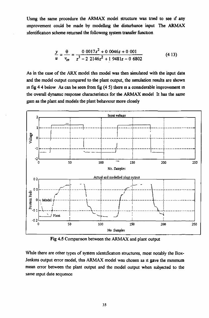
Using the same procedure the A R M A X model structure was tried to see if any improvement could be made by modelling the disturbance input The A R M A X identification scheme returned the following system transfer function

v 0 0 0017z2 + 0 0046z + 0 001— = — = 5-------------------- (4 13)« V,„ Z3 - 2 2146z2 + 1 948 lz - 0 6802

As in the case of the ARX model this model was then simulated with the input data and the model output compared to the plant output, the simulation results are shown in fig 4 4 below As can be seen from fig (4 S) there is a considerable improvement in the overall dynamic response characteristics for the A R M A X model It has the same gam as the plant and models the plant behaviour more closely

Input voltage

BO3 o

-2

q h ....;....

i.......►.....

50 100 ~ 150

No. Samples

Actual and modelled plant output

200 250

100 150

No Samples

Fig 4.5 Comparison between the A R M A X and plant output

While there are other types of system identification structures, most notably the Box- Jenkms output error model, this A R M A X model was chosen as it gave the minimum mean error between the plant output and the model output when subjected to the same input date sequence

35

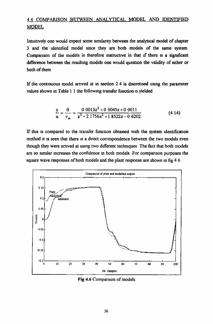
4 4 COMPARISON BETWEEN ANALYTICAL MODEL AND IDENTIFIEDMODEL

Intuitively one would expect some similarity between the analytical model of chapter 3 and the identified model since they are both models of the same system Comparison of the models is therefore instructive in that if there is a significant difference between the resultmg models one would question the validity of either or both of them

If the continuous model arrived at m section 2 4 is discretised using the parameter values shown in Table 1 1 the following transfer function is yielded

y _ _0_ _ 0 0013z2 + 0 0045Z + 0 0011u “ vm “ z3 - 2 1756z2 +1 8 5 2 2 z -0 6202 '

If this is compared to the transfer function obtained with the system identification method it is seen that there is a direct correspondence between the two models even though they were arrived at using two different techniques The fact that both models are so similar increases the confidence in both models For comparison purposes the square wave responses of both models and the plant response are shown in fig 4 6

36

From fig 4 9 it can be seen that both model types give a good characterisation of the plants response On closer inspection it may be seen that the A R M A X model gives a closer match to the plant output especially during the dynamic response It is this model therefore which is used as a description of the plant

4 5 TRANSFER FUNCTION TO STATE SPACE TRANSFORMATION

The models presented in equations (4 12) to (4 14) above are in transfer function form This is suitable for input-output data, but from the discussion in chapter 3 we see that a state-space representation is required if the designer is to have access to the internal system states, The estimator is also designed with the state space format in short this necessitates a transformation from transfer function to state space representation

Although there are standard transfer function to state space transformation CAD routmes, the transformed state space representation is usually in controller canonical form where the states are derivatives of the measured output state This has a limited physical meaning to our present application where we choose position, velocity and current as the three states We must therefore transform from the canonical basis to our desired physical state vector basis This is done by selecting the transformation matrix M such that1 __

w = Mx (4 15)

where x is the state vector [0(k) 0(k + l) I(k)]T and w is the 3*1 canonical state matrixIf the canonical state space representation is given as

w(k + l) = <X>w(k) + Tu(k)' \ i \ i ( 4 1 6 )

y(k) = Nw(k)

then the required state space representation under the basis transformation of (4 15) is given as

1 This approach has a heuristic reasoning in transforming from the physical to the canonical transformations

37

x(k + l) = M '<I>Mx(k) + MTu(k) y(k) = NMx(k)

A more detailed diagram showing the various steps in completing this transformation is shown in appendix A 2

4 6 S U M M A R Y

This chapter discusses the importance of a good system model, this is especially important in the context of sensorless control which is discussed in later chapters The system identification method was implemented for the voice coil actuator scanning system The derived models were then compared and found to be similar to the models derived analytically This promoted confidence in the models which was justified since both could reproduce the plant output to given excitation signals with a high degree of accuracy It was concluded however that the A R M A X system identification method gave an overall better model The transformation from the transfer function model to the required state space basis was then discussed

38

CHAPTER 5

CONTROLLER DESIGN

5 I INTRODUCTION-

In chapter 3 the design alternatives were introduced as two basic categories, these being the classical transfer function and modem state space control methods respectively Emulation, where the design is earned out m the s- plane and the fact that the controller is implemented in discrete time is cited as bemg a useful exercise [5-1] This produces a good controller when the sampling frequency is many times (approximately 30) greater than the system bandwidth, but this design is usually used as a guide for more detailed direct digital design and is used as an aid in selecting the sample frequency

The purpose of this chapter is to show in detail the design of the digital controller (desenbed m chapter 3) which will be implemented on the actual galvanometer ng

5 2 CONTROLLER ROOT SELECTION- -

5.2.1 Introduction

As was stated in chapter 3 the systems dynamic response charactenstics are dictated by the position of the closed loop poles and zeros One of the major strengths of state space design over its transfer function compensator equivalent is that the systems poles can be placed at any arbitrary position (within reason) Therefore the design consists of selecting appropnate root locations which meet a set of specifications which define the overall system performance in terms of certain measurable quantities Typical examples of which include damping, nse time, settling time, percent overshoot and steady state error All these quantities must be satisfied simultaneously in the design which results in the design becoming a tnal and error procedure

To help the design process to become more methodical, in identifying the relative performance of a set of root locations it is usual to define a Performance Index. These

39

indices are based on functions of the variable system parameters Minimum or maximum value of this mdex then corresponds to an optimum set of parameter values As well as providing a single figure of ment for a set of root locations other advantages of performance indices are their ease of analytical computation, sensitivity to parameter variations and ability to distinguish between desirable and non-desirable root locations

5.2.2 The ITAE criterion

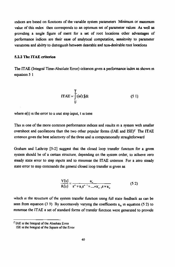
The ITAE (Integral Time-Absolute Error) criterion gives a performance index as shown m equation 5 1

ITAE- t(e(t|di (5 1)O'

where e(t) is the error to a unit step input, t is time

This is one of the more common performance indices and results m a system with smaller overshoot and oscillations than the two other popular forms (IAE and ISE)r The ITAE criterion gives the best selectivity of the three and is computationally straightforward

Graham and Lathrop [5-2] suggest that the closed loop transfer function for a given system should be of a certain structure, depending on the system order, to achieve zero steady state error to step inputs and to minimise the ITAE criterion For a zero steady state error to step commands the general closed loop transfer is given as

= ________5 ________ (52)K(s) s“ :F'dls ‘I 1 '+~~+an ,s + a;r

which is the structure of the system transfer function using full state feedback as can be seen from equation (3 9) By successively varying the coefficients a„ in equation (5 2) to minimise the ITAE a set of standard forms of transfer function were generated to provide

r IAE is the Integral of the Absolute Error ISE is the Integral of the Square of the Error

40

a suitable set of closed loop root locations.For the transfer function of equation (3 9) the Following equation gives the corresponding'minimum ITAE set of root locations as having the characteristic equation

s4 +‘2 IoJns3 + 3.4© n2s2 +'2.7con3s +"torn4 - 0 (5 3)

where tD It is the undamped natural frequency and is given as

c (5VK=Spnng stiffness JMnertia

Using' equation (5.4) in equation (5 3) yielded the Following set oF desired continuous closedToop pole locations

-1 11 *10* ±'3 31*10 7(5 5)

-1 64*10311 08752* 10?j

It is noted that there are Four root locations specified here even though the open loop system is oFthird order.As explained m chapter 3 the extra poFe location comes from the additional augmented mtegraF state.

5.2.3 Ackermanns Formula

Given aset of desired root locations (For example by usingthe ITAE criterion above) the question oF what Feedback gams move the systems closed loop poles to these locations then arises. One oF the advantages oF fuff state Feedback design with a state space representation was stated as being its suitability For use in CAD routines. AT compact Formulation,, suitable For CAD environments was developed by Ackermann [5-1] For the purpose oF’caFcuFating a set oFFeedback gams given corresponding" to a set oF clesired pole locations .The Formula is repeatedhere as

K -[0 . _ . 0 f][B AB A*B _ _ . A" 'B] !ar(A) (5 6)

41

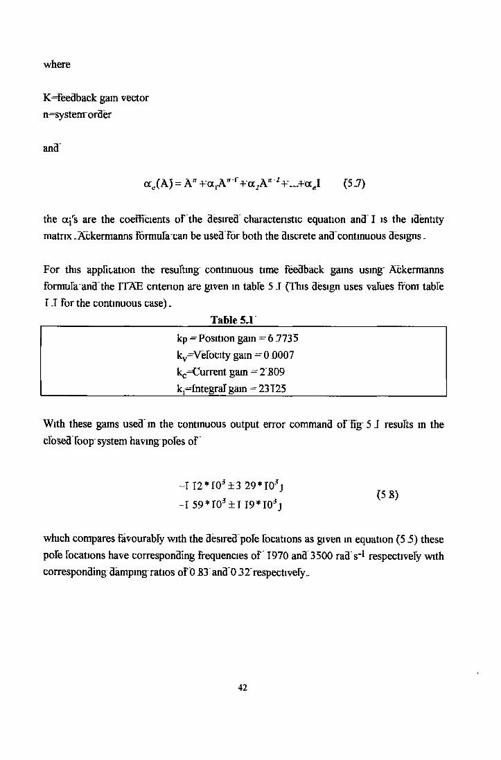
where

K^Feedback gain vector n^ystemorder

and

oc,(A J = A 11 +a1A ‘ir+-azA"'z+-„.+aII (5 „7)

the eel's are the coefficients of the desired characteristic equation and I is the identity matrix.Ackermanns Formula can be used For both the discrete and'continuous designs.

For this application the resulting continuous time Feedback gams using' Ackermanns Formula and the ITAE criterion are given in table 5 J (This design uses values from table IJ For the continuous case).

Table 5,1kp - Position gain =6.7735 kv̂ Velbcity gain - 013007 kc-=Current gain - 2 E09 k̂ integral' gain ̂ 23125

With these gams used in the continuous output error command oF fig 5 J results in the closedToop system having poles oF

-1 12*10 + 3 29*10 j* (5S)- I 5 9 * 1 0 + 1 1 9 * 1 0 j

which compares Favourably with the desired pofe locations as given in equation (5 5) these pofe locations have corresponding frequencies oF 1970 and 3500 rad s'1 respectively with corresponding damping ratios oFO S3 and 0 32 respectively»

42

This continuous system is then simulated using the Mathworks SIMULINK package in conjunction with the Control Systems Toolbox [5-3] using a Runge-Kutta 5^ order numerical integration scheme The system response to a desired position of 0 1 rad is shown in fig 5 2 below

Fig 5.2 Step response using ITAE criterion

43

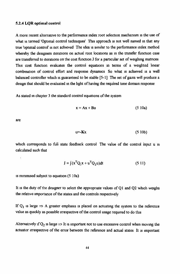
5.2.4 LQR optimal control

A more recent alternative to the performance index root selection mechanism is the use of what is termed 'Optimal control techniques' This approach is not well named in that any true 'optimal control' is not achieved The idea is similar to the performance index method whereby the designers iterations on actual root locations as in the transfer function case are transferred to iterations on the cost function J for a particular set of weighing matrices This cost function evaluates the control equations m terms of a weighted linear combination of control effort and response dynamics So what is achieved is a well balanced controller which is guaranteed to be stable [5-1] The set of gains will produce a design that should be evaluated in the light of having the required time domain response

As stated in chapter 3 the standard control equations of the system

x = Ax + Bu (510a)

are

u=-Kx (5 10b)

which corresponds to full state feedback control The value of the control input u is calculated such that

J = j ( x ^ x + uTQ 2u)dt (5 11)

is minimised subject to equation (5 10a)

It is the duty of the designer to select the appropriate values of Q1 and Q2 which weighs the relative importance of the states and the controls respectively

If Ql is large => A greater emphasis is placed on actuating the system to the reference value as quickly as possible irrespective of the control usage required to do this

Alternatively if Q 2 is large => It is important not to use excessive control when moving the actuator irrespective of the error between the reference and actual states It is important

44

therefore that the control input weighting matnx Q2 is given some weighting since if the calculated control input was excessive there is a possibility that the actuator may become saturated or in some cases damaged

Equation (5 11) subject to equation (5 10) is a 'standard constrained minima' problem which is solved using the method of Lagrange multipliers

The Lagrange method consists of writing equation (5 10a) and (5 10b) as

j' = J[IxTQ 1x + iuTQ 2u + XT(-x + Ax + Bu)] (5 12)

taking the partial derivatives of this equations with respect to the three quantities of interest results in [5-4]

di'— = utQ 2 + XtB = 0 control eqns (5 13 a)duôy— = -x + Bx + Bu = 0 state eqns (5 13b)dX

dy— = xtQ j - A.t + XA = 0 adjoint eqns (5 13c)dx.

Solving these equations subject to certain boundary conditions results in the following time varying solution for K(t)1

K(t) = [Q2 + B TS(t)B]~1 B TS(t)A (5 14)

where S is found by solving the Riccati equation

0 = SA + A TS - SBQ2" *S + Qj (5 15)

As stated above this is a time varying solution, although when these equations are implemented it is noted that they quickly converge to a steady state value Therefore to compute the value of K one looks for the steady state solutions for equation (5 15) by

1 A full discussion is given m Bryson and Ho [5-5]

45

realising that in the steady state S(t) is the same as S(t+1) a unit time later, both of which are now called S«, The LQR steady-state Riccati equations are given as

s. = AT[S„ - S„BQ2- 'Bt S J A + Q, (5 16)

resulting m the following LQR steady state control equations

K 00 = (Q2 + B tS00B)-1BtS00A (5 17)

These are implemented on the MATLAB CAD package, for the galvanometer scanner the weighting matrices were chosen to give a fast dynamic response The calculated controller gains are shown in table 5 2

_______________________________ Table 5.2____________________________________

kp = Position gain = 24 91 kv=Velocity gain = 0 0056 kc=Current gain = 3 17

______________________k̂ Integral gain - 55000__________________________

The step response to a step reference is shown in fig 5 3 and shows a faster travel time to that of the ITAE method and also the overshoot is significantly reduced These gains resulted the system having following closed loop pole locations

-110* 103 ± 4 49*103j(5 18)

-1 89*±1 40*10 j

with corresponding damping factors of 0 23 and 0 803 respectively

46

Response using LQR algorithm

Time mS

Fig 5.3 Response using LQR design

5 3 SAMPLE RATE SELECTION

5.3.1 Introduction

The designs earned out thus far have been in the continuous S-domain This is a useful exercise since it gives the designer the flexibility to carry out the design without having to specify the sample rates But since the final controller is being implemented m discrete time it is necessary at some stage to select the sample rate at which the controller will operate

As in most designs the selection of the 'optimum' sample rate is a compromise between several key elements the two primary ones being cost versus performance In typical design situations the target processor is specified before the control engineer has formulated what is the ideal, most cost effective approach The target processor available for this proto-type application is the Texas Instruments third generation TMS320C30

47

digital signal processor (DSP) This platform automatically dictates the system word size, (32 bit floating point arithmetic), and the A/D precision (16 bit) as well as the maximum throughput sampling rate (200 kHz) However, usually the best choice is to choose the slowest sample rate that meets all performance requirements

5.3.2 Signal smoothness

The well known sampling theorem sets the absolute lower bound on the sampling rate as

> 2 (5 19)4

where fs is the sample rate and f̂ is the closed loop bandwidth This means that in order to reconstruct a band limited1 continuous signal we must sample at least twice as fast as the highest frequency component in that signal For the digital controller to have a performance comparable to its analogue equivalent the required closed bandwidth is approximately 300 Hz, which means that the lowest theoretical sampling frequency would be 600 Hz This lower limit is practically never used m real applications as it would be deemed too slow to provide a suitable time response and also the signal smoothness would usually be inadequate Franklin and Powell [5-1] suggest that a good rule of thumb to provide a reasonably smooth time response is to select the sampling frequency in the range

6 < — < 40 (5 20)fb

The smoothness for a variety of sampling frequencies are shown in Appendix B The required smoothness depends on the actuator and the application, for example a lift carrying passengers would require smooth journey whereas smoothness might not be an issue when moving product along an assembly line The smoothness requirements for the scanner are moderate, (in fact electric motors can handle large discontinuities) although large excursions in output should be avoided Many DSP's, as does the TMS320C30, possess lowpass filters between the digital to analogue converter (DAC) and the actuator

1 All mechanical systems exhibit low pass filter characteristics

48

input to help reduce the effect of the discontinuities The TMS320C30 uses a 4th order Sallen - keylow pass filter with a variable cutoff frequency

5.3.4 Noise and Antialiasing filters

Although electronic design should be earned out so as to minimise the effect of external disturbances, for example shielding to help reduce electro-magnetic interference, proper grounding to eliminate differences m voltage references and isolating high power/frequency circuits from their low power/frequency counterparts, notwithstanding these precautions a certain amount of noise will exist in any real circuit [5-6]

High frequency disturbances (outside the system bandwidth), through a phenomenon known as signal aliasing, can be transferred into a lower frequency range by the sampling process Consider the continuous signal s(t) which is sampled with a sampling penod T

i

sk = s(kT), k = l,2, (5 21)

Then the sampling frequency is given cos = ~̂ ~ and the nyquist frequency as © N =^-

from the sampling theorem it is known that a sinusoid with frequency greater than © N when sampled, be distinguished from one in the interval [-oN,coN] Therefore part of the signal spectrum that corresponds to frequencies higher that coN will be interpreted as contnbutions from lower frequencies

This aliasing effect can be significantly reduced through the use of Antialiasing filters or prefilters These prefilters are low pass filters used to suppress high frequency noise components above the prefilter breakpoint fp The prefilter has an effect on sample rate selection since the prefilter breakpoint must be sufficiently faster than the system bandwidth f̂ such that the phase lag introduced by the prefilter does not significantly change the system stability It is suggested [5-1] that for a good reduction in the high frequency noise at fs/2 the sample rate selected should be approximately four to five times the prefilter breakpoint

From a consideration of the above it was decided that a good compromise was to select the sample frequency as

49

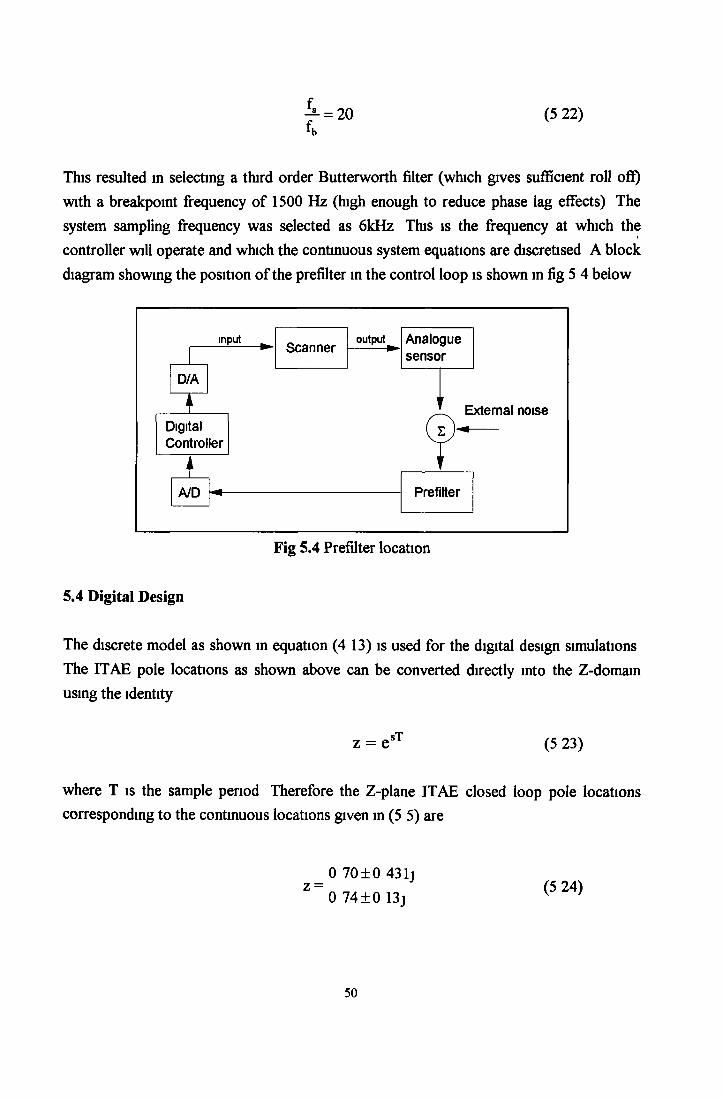
f— = 20 fb

(5 22)

This resulted in selecting a third order Butterworth filter (which gives sufficient roll off) with a breakpoint frequency of 1500 Hz (high enough to reduce phase lag effects) The system sampling frequency was selected as 6kHz This is the frequency at which the controller will operate and which the continuous system equations are discretised A block diagram showing the position of the prefilter in the control loop is shown in fig 5 4 below

inputScanner

output Analoguesensor

D/A

External noiseDigitalController

A/D Prefilter

Fig 5.4 Prefilter location

5.4 Digital Design

The discrete model as shown in equation (4 13) is used for the digital design simulations The ITAE pole locations as shown above can be converted directly into the Z-domain using the identity

z = esT (5 23)

where T is the sample period Therefore the Z-plane ITAE closed loop pole locations corresponding to the continuous locations given in (5 5) are

0 70 + 0 43 lj z = (5 24)0 74±0 13j V '

50

As stated earlier Ackermanns formula is suitable for both continuous and discrete time Therefore when used with the discrete system with the required root locations as in (5 24) the following discrete feedback gains are produced

_______________________________ Table 5.3____________________________________

kp = Position gain = 6 9481 kv=Velocity gain = 0 000207 kc=Current gam = 1 926

______________________k,=Integral gain = 18683__________________________

The above feedback gains produce the following simulation response

Digital response with ITAE criterion

Time mS x lO 3

Fig 5.5 Response of Digital controller using the ITAE criterion

51

5.4.1 Direct digitai design

There are several methods of direct digital design, firstly one could transform the system specifications into the discrete domain and use one of the discrete transfer function methods such as discrete root locus, Bode or Nyquist techniques. Since we are looking at state space full state feedback control (as justified in chapter 3) we will use a method appropriate to this approach. This involves using the discrete linear quadratic regular equations. These are formulated in exactly the same way as for the continuous design and are used to calculate the discrete control feedback matrix K. In the discrete case the cost function

Jdis = I 2 fxT(k)Q,x(k) + uT(k)Q2u(k)| (5 .2 5 )k=0

subject to the constraint

-x (k +1) + Ax(k) + Bu(k) = 0, k = 0 ,l,. . „ N 1 (5.26)

As in the continuous case the discrete LQR solution converges to a steady state value, so it is this value which is used in the controller, so the steady state discrete solution is given as [5-1]:

K m = (Q2 + BTS00B)- ‘B X A (5.27)

Where S« is the solution to the steady state discrete time Riccati equation

S» = AT[SW - S00BQ2BTS00]A + Q2 (5.28)

This algorithm was implemented for the digital controller and gave the followingcontroller gains. The LQR digital design methodology gave a better response than theITAE design as can be seen from fig 5.6 below.

1 Whenever we talk about discrete time it is assumed that A, B ,C and D system matrices are the discrete versions of their continuous counterparts.

52

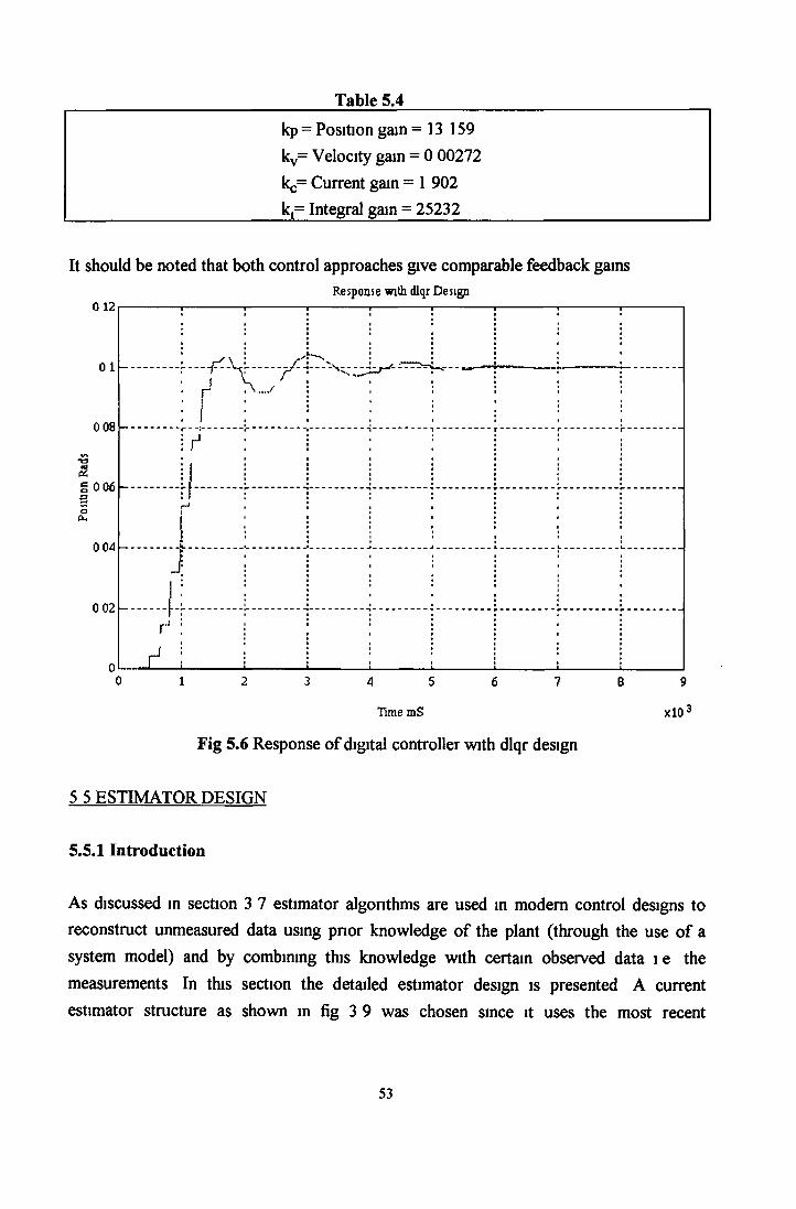
Table 5.4

kp = Position gain =13 159 kv= Velocity gain = 0 00272

kc= Current gain = 1 902 kt= Integral gain = 25232

It should be noted that both control approaches give comparable feedback gainsResponse with dlqr Design

TimemS xlO3

Fig 5.6 Response of digital controller with dlqr design

5 5 ESTIMATOR DESIGN

5.5.1 Introduction

As discussed m section 3 7 estimator algorithms are used in modem control designs to reconstruct unmeasured data using prior knowledge of the plant (through the use of a system model) and by combining this knowledge with certain observed data i e the measurements In this section the detailed estimator design is presented A current estimator structure as shown m fig 3 9 was chosen since it uses the most recent

53

measurements and hence produces the fastest response to unknown disturbances and unmodelled measurement noise The current estimator equations are given again as

x(k) = x(k) + L(y(k) - Cx(k)) (5 29a)

x(k) = Ax(k -1) + Bu(k -1) (5 29b)

Where x(k) is the current estimate based on the current measurement y(k) and x(k) is the prediction estimate based on the previous estimate at time k-1 From the error equation for this estimator, given in equation (3 20), it can be seen that by selecting an appropriate matrix L it is possible to control the dynamics of the error equation No model is perfect and no measurement is completely noise free so realistically the estimator will never exactly match the actual system states Therefore the aim of the estimator design is to keep these errors sufficiently small for the required application

5.5.2 Selection of estimator gains

The selection of the estimator gains is similar to that for the control case where a particular choice of L will place the closed loop estimator error roots at a corresponding location which is reflected in the dynamics of the error (as stated in chapter 3) If sensor noise is significant and the plant model is good then it is best to rely on the plant model and regard the measurements with a certain degree of scepticism This is equivalent to reducing the estimator gains

From the above discussion it is clear that there is a link between the selection of the estimator gains and the merit of the plant and sensor measurements The preferred choice would be to choose the estimator gains so as to minimise estimator errors taking the sensor and modelling errors into account This approach was formalised by Kalman in 1962 resulting in the stochastic Kalman Filter solution [5-8]

5.5.3 The discrete Kalman filter

The Kalman filter is a stochastic algorithm in that it is designed with the noise characteristics of the system in mind In terms of system noise components the discrete plant may be written as

54

x(k + l) = Ax(k) + Bu(k) + Gw(k) (5 30a

with the output

y(k) = Cx(k) + v(k) (5 30b)

where w(k) is the process noise and v(k) is the measurement noise Both of these quantities are assumed to be uncorrelated random variables with zero mean, or

where E{»} is the expectation operator These quantities have covariance's of Rw and Ry respectively, and are defined as

In choosing the value of L in equation (5 29a) above, we want to update the previous estimate of equation (5 29b) with the current measurement based on the relative accuracy of the two quantities Kalman formulated his solution based on the least squares concept to minimise the mean-square measurement errors In conjunction with this, a priori knowledge of the system (i e the system model) is used to predict system behaviour between measurements The development of the Kalman filter can be found in [5-7],[5-8] and is not repeated here However the final Kalman solution is presented here for completion

The measurement update equation is given as

Where P(k) is the estimator covariance immediately after a measurement and is defined as

E{w(k)} = E{v(k)} = 0 (5 31)

R w = E{w(k)wT(k)} and R v = E{v(k)vT(k)} (5 32)

x = x + P(k)CTR^ (y(k) - Cx(k)) (5 32)

P(k) = M(k) - M(k)CT(CM(k)CT + R v)_1 CM(k) (5 33)

and the time update equation is

55

x(k +1) = Ax(k) + Bu(k)

M(k) in equation (5 33) is the estimator covariance which gives a figure of ment for the estimates just before the measurements at time k are taken M(k) is therefore an updated version of P(k) and is given as

M(k +1) = AP(k)AT + G R wG t (5 35)

By comparing equation (5 29a) to (5 32) we see that the estimator gain L is given as

L(k) = P(k)CTR~1 (5 36)

From (5 36) it is obvious that the gain L is parametensed by k and therefore vanes with time However, as in the controller case, the value of L will converge to a steady state value In fact the steady state Kalman equations are denved in much the same way as for the steady state control equations, l e by letting L(k)=L(k+1 )=L00 and forming thecorresponding Riccati equations Following this approach results in the following steady state Kalman filter gams

L „ = M „ C t(CM.Ct + R i)-1 (5 37)

This value can then be determined off-line, which greatly reduces the computational complexity as compared to performing the relatively complex equations (5 33) and (5 35) on-line

5.5.4 Selection of Ry and Rw

The ratio of the matnces Ry and Rw in the Kalman equations dictates the closed loop estimator dynamics The selection of Ry can be given a physical interpretation as depending on the sensor noise For example the RMS noise level specified for many sensors is simply squared to amve at the diagonal elements of E{v2(t)} or from observation of the sensor noise levels an approximate value for Ry can be obtained A typical noise sequence is the sensor is shown in fig 5 7 below

56

xlO -3 MeaiuiemeatQOKc corintnce of te 9

Samples

Fig 5.7 Measurement noise levels

The selection of Rw is more abstract in that it is accounting for unknown disturbances such as process noise or plant model imperfections The actual values of Rw are selected such that no modes of the estimator are without feedback so that the estimator will track all system states Often the value of Rw is selected on the quality of results obtained from simulation when all known disturbances are included

Another factor in selecting the value of Rw is the location of the resulting estimator error closed loop poles From the separation principle, equation (3 27) we see that the closed loop system poles are made up of the control and estimator error poles Therefore it is usually desirable to have the estimator poles at least as twice as fast as the controller poles so that the system response is dominated by the controller poles1

Taking the above factors into consideration the LQED (Linear Quadratic Estimator design for the Discrete case) algorithm was used to calculate the discrete constant Kalman gains for this system The selected gains were calculated as being 0 7, 2367 2 and 1 4 for the position, velocity and current states respectively These gains give error dynamics with equvalent continuous frequencies of 7598, 7598 and 6506 rad s'1, each of which are faster than the closed loop controller roots which is usually desirable

1 There are exceptions to this norm, for example in regulator plants with a good system model and noisy sensor measurement data it may be desirable to have the estimator poles slower that the control poles so that good measurement filtering is performed

57

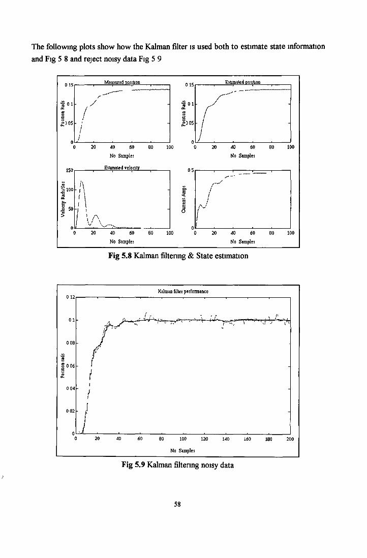
The following plots show how the Kalman filter is used both to estimate state information and Fig 5 8 and reject noisy data Fig 5 9

0 15

01

>)05

1 1 ! ■ 1 0 15 " 1 * 1 1----1 " i--- *

- yt - Ü 01 £

1 \ -

1 aea /i - £ 3 05

/" / -

/t i

/

J — . 0 /

150

tlOO

50

20 40 60 80 100

No Samples

Estimated velocity

20 40 60

No Samples

I t

20 40 60 eo

No Samples

100

No Samples

80 100

Fig 5.8 Kalman filtering & State estimation

58

5 6 SENSORLESS CONTROL

5.6.1 Introduction

Several transducer types are commonly available for sensing rotary angles, typical sensors include

• Capacitive sensors• Potentiometnc sensors• Differential transformers• Optical encoders• Resolver• Interferometers

Each of these transducers have relative advantages / disadvantages m relation to accuracy, inertia and cost [5-9] In this section we will look at an alternative control approachapplicable to the galvanometer system which involves the elimination of the above electro­mechanical sensors altogether

Direct measurement of rotor position is expensive, manufacturing, mounting and maintenance requirements are increased as is the rotor inertia However, motor current is easily measured and if the galvanometer dynamics are sufficiently well known then the position and velocity information may be determined in an indirect way [5-10] This gives rise to a control strategy known as sensorless control

From the work presented thus far a mechanism for determining unknown data from observed measurements and additional knowledge of the behaviour of the system via the plant model (l e The state estimator/Kalman filter approach) was presented This approach will now be used as a means of providing sensorless control

5.6.2 The sensorless topology

From chapter 4, where the issue of system identification was presented the importance of obtaining a good system model was stressed, this section also discussed the formulation of the state equations where the selected states of position, velocity and current, gave an

59

explicit relationship between current, the measured quantity for sensorless control and the states of interest 1 e position and velocityWhen using the sensorless control method the state equations are slightly changed to inform the Kalman filter that the measured quantity is now current and not position so

y = [0 0 l]e0I.

(5 38)

The discussion of the state estimator/Kalman filter applies equally to the sensorless case as does the selection of the controller structure- the difference being that the position and velocity being fed back are measured quantities The controller-estimator topology employed for the sensorless control case is shown in fig 5 8 below

Fig 5.8 Sensorless topology

5.6.3 Simulation results

The above controller/estimator has been simulated using the SIMULINK CAD tools The results obtained indicate the validity of this control technique to voice-coil motor applications as m laser scanning and disk drive systems The results show that the system can track a desired position reference with ideally zero steady state error, and has a bandwidth comparable to the equivalent system with a position sensor Fig 5 9 below shows the simulation results obtained for the constant gain Kalman filter following a square wave input without using a position sensor This method is implemented in chapter

60

6 and results obtained which validate the sensorless approach for certain types of applications

5 7 S U M M A R Y

This chapter deals with the issues involved in carrying out a detailed controller design First the idea of root selection is discussed and two different methodologies are presented for the selection of satisfactory closed loop root locations Two controller designs, corresponding to the ITAE and LQR methods are presented in both the continuous and discrete domains These controllers are implemented in the next chapter

The sample rate selection issue was then presented in terms of both signal smoothness and anti-aliasing filter design The state estimator, as outlined in chapter in chapter 3 was then designed using the Kalman filter approach where the selection of the estimator gains was viewed in terms of the merit of the plant and sensor measurements the overall objective being to minimise estimator errors

Sensorless control was presented, where it was proposed that control could be exercised over voice coil actuators without using any direct position/velocity transducers The idea is based on the state estimator where knowledge of the plant and certain indirect measurements are used to estimate or reconstruct the unmeasured states of position and velocity

61

CHAPTER 6

SYSTEM IMPLEMENTATION

6 1 INTRODUCTION

In the previous chapter the detailed design of the controller from the continuous domain through to the discrete z-plane was described The issue of sampling frequency was discussed and a sampling interval selected This chapter deals with the practical implementation of the digital design which, up to now involved computer simulation The issues of hardware and software are discussed ranging from the ' design of the plant and sensor interfaces through to the control algorithm formulation and testing Control is exercised both with and without the use of position sensors, with results presented for both controller types

6 2 HARD W A R E

6.2.1 Description

For this proto-type application the General Scanning G120D scanner is used, a description of which is presented in section 2 3 The primary function of this actuator is to deflect an incident beam and exercise control over the resultant position of this beam relative to some reference framework This type of scanner is in wide commercial use in such applications as laser display projection, non impact printing, infrared detectors and space communications For illustration purposes a simplified laser projection rig (as frequently used in the entertainment industry), is shown in fig 6 1 below One can easily visualise that as the scanner rotates the laser beam traverses the screen giving the required scanning action

62

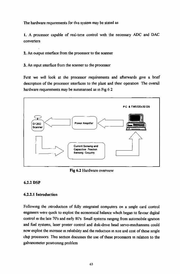
The hardware requirements for this system may be stated as

1. A processor capable of real-time control with the necessary ADC and DAC converters

2. An output interface from the processor to the scanner

3. An input interface from the scanner to the processor

First we will look at the processor requirements and afterwards give a brief description of the processor interfaces to the plant and their operation The overall hardware requirements may be summarised as in Fig 6 2

6.2.2 DSP

6.2.2.1 Introduction

Following the introduction of fully integrated computers on a single card control engineers were quick to exploit the economical balance which began to favour digital control in the late 70's and early 80's Small systems ranging from automobile ignition and fuel systems, laser printer control and disk-dnve head servo-mechanisms could now exploit the increase in reliability and the reduction in size and cost of these single chip processors This section discusses the use of these processors in relation to the galvanometer positioning problem

63

6.2.2.2 Processor requirements

1. Speed

The fundamental cntenon for processor speed is that enough time must be available to complete the control equations before the arrival of the next sampled data or as soon as possible As well as the possibility of losing input data too much delay in the controller output may introduce excessive phase delay into the system which could lead to instabilities Many of the general purpose processors used to implement controllers are usually too slow to process signals m real time, relying instead on pre­computed lookup tables limiting their operation to low-performance or low bandwidth systems [6-1] Therefore as faster mechanical systems are included in the digital control arena, (and the galvo scanner is ranked among these), then greater performance is demanded from the control processors

This has led to the development of high specification dedicated digital signal processors (DSP's) specifically designed for the high data throughput associated with digital signal processing and control applications

2 Word length

By their very nature, numbers1 used in digital control must fit into words of finite length, usually expressed as the width of the data stream in bits This discretization or loss of resolution is known as quantization error For a fixed point representation (see below) the accuracy achieved is decided by the quantum size q, where q is given as

q = 2-L (6 1)

Where L is the word length As well as the quantization effect, results of mathematical operations must also fit within the word length and therefore the resultant accuracy is reduced by this truncation/rounding process If these effects are significant then they may cause oscillations or limit cycles which can lead to instability

The problems discussed above are only significant in processors that have 8/16 bit ALU's and registers

1 By 'Numbers' we are referring to any quantity that is represented internally in the computer, these quantities may be sampled signals, parameter co-efficients or system gams

64

3 Data representation

Another important factor is how are the data represented, two basic formats exist

A. Fixed pointFixed point representation is where each number is represented with a fixed location for the binary equivalent of the decimal pomt This produces correct results when the operation being performed yields results which are within the limits of the representation If the results extends beyond this upper/lower limit then numerical overflow results, since most processors Wrap-Around' when this occurs the output swings from its max [min] to its min [max] levels causing the output to reverse direction Overflow must be avoided by employing amplitude scaling, or if it is allowed to exist must be modelled as a major non-lineanty (depending on whether a wrap-around or saturation scheme is used in the registers)

B. Floating pointThis method uses three numbers, m the mantissa, c the characteristic and b the base Using this format a given number n is represented as

n = m *bc (6 2)

For the floating pomt representation the precision is not absolute (as in fixed point) but relative It can be shown that relative error is bounded by

^ V r ^ b 1_nm (6 3)M

where the number n is represented as n= m*bc and nm is the number of bits In practical control applications using the floating point format with nm as low as 24 bits produces quantization errors which are negligible in comparison to other noise sources [6-2]

Floating point representation is therefore usually preferred by system designers due to its extended dynamic range and its ease of design when compared to the fixed processor types1 The penalty for a floating point device is increased cost and power

1 With floating point arithmetic high level language can be used directly without having to do the number scaling which is associated with fixed point processors

65

dissipation, notwithstanding these drawbacks floating point arithmetic is the trend for DSP chips

From the above discussion it clear that speed, word size and data representation are all key factors in selecting a processor for high bandwidth real-time processing It was also stated that these requirements brought about the development of DSPs and that these DSPs can significantly reduce or eliminate the problems encountered when using standard 8/16 bit micro-processors

A typical DSP platform, and the one that is used in this implementation, is the TMS320C30 system In the next section a brief overview of some of the key features of this DSP are presented including the CPU performance, system memory and the analogue I/O interface

6.2.2.3 The TMS320C30

The TMS320C30 is a high performance CMOS DSP and is used in a wide variety of applications More specifically it has an optimised architecture which uses both the Harvard and von Neumann types, a dedicated hardware multiplier, extensive four phase pipe lining in parallel, a powerful DSP instruction set and a fast instruction cycle All these features give it the high-speed number crunching capabilities ideal for real-time servo-motor control

The TMS320C30 board is comprised of the TMS320C30 processor, a two channel 16-bit A/D - D/A interface, expansion memory, a PC interface with parallel and serial expansion slots The boards internal bussing and instruction set gives it a 33 3 MFLOPS (million floating-point computations per second) processing capability formerly only available on a super computer [6-3]

6.2.2.4 The TMS320C30 CPU

The TMS320C30 DSP is an extremely fast processor, the instruction cycle time of 60 nanoseconds giving the processor an execution rate of 16 7 MIPS ( Millions of instructions per second) The processor provides 32-bit words consisting of program, data and I/O space The 32-bit words are in floating point format with an 8 bit exponent and a 24 bit mantissa The processor has a 32-bit integer / 40-bit floating point multiplier and ALU

66

The processor has a high degree of parallelism and perform parallel multiply and ALU operations in a single cycle The processor also has a general purpose register file which supports addressing, floating point/integer operations, stack management, processor status, block repeats and interrupts The 64*32-bit instruction cache minimises the number of off chip accesses by storing often repeated sections of code and allows code to be stored in slower (and cheaper) off-chip memories The processor also has one D M A channel, internal dual-access memories and a short machine cycle

The TMS320C30 DSP provides a powerful solution to most modem control/DSP requirements by providing a high degree of innovative integration it combines the high performance CPU with two external interface ports, large memories, efficient buses, D M A controller, two serial ports, two timers and a multiple interrupt structure

6.2.2.5 System memory

The 24-bit address bus gives the TMS320C30 a total memory space of 16* 106 32-bit words allowing tables, co-efficient, program code or data to be stored in either R A M or R O M The R A M blocks 0 and 1 are lK*32-bits each and the R O M block is 4K*32-bits Each of these memory types allows two CPU accesses in a single cycle The separate program and data buses provided allow for parallel program fetches, data reads/writes and D M A operations

6.2.2.6 Memory Maps

The memory map depends on whether the processor is operating in the micro­processor mode or the micro computer mode The memory maps for these modes are similar, the main difference is that for the micro-processor mode the 4K on-chip R O M is not mapped into the TMS320C3x memory map The memory maps for both these modes are shown in fig 6 3a and 6 3b below

6.2.2.7 Reset/Interrupt/Trap Vector Maps

The addresses for these vectors are mapped into the address OH through to 3FH These vector addresses contain the starting addresses of the respective reset, interrupt and trap routines These vector mappings are shown in fig 6 4 below

67

OHOBFH

Interrupt Locations and Reserved (192)

OCOH7FFFFFH

External STRB Active

800000H801FFFH

Expansion Bus MSTRB Active (8K)

802000H803FFFH Reserved (8K)

804000H805FFFH

Expansion Bus IOSTRB Active (8K)

806000H807FFFH Reserved (8K)

808000H8097FFH

Peripheral Bus Memory- Mapped Registers (6K)

809800H809BFFH

R A M Block 0 (lK)Intemal

809C00H809FFFH

R A M Block 1 (lk)Intemal

80A000HOFFFFFH

External STRB Active

OHOBFH

Interrupt Locations and Reserved (192)

OCOHOFFFH

ROM(IntemaI)

1000H7FFFFFH

External STRB Active

800000H801FFFH

Expansion Bus MSTRB Active (8K)

802000H803FFFH

Reserved (8K)

804000H805FFFH

Expansion Bus IOSTRB Active (8K)

806000H807FFFH

Reserved (8K)

808000H8097FFH

Peripheral Bus Memory- Mapped Registers (6K)

809800H809BFFH

R A M Block 0 (lK)Intemal

809C00H809FFFH

R A M Block 1 (lk)Intemal

80A000HOFFFFFH

External STRB Active

Fig 6.3a Microprocessor Mode Fig 6.3b Micro-Computer Mode

6.2.2.8 Peripheral Bus Map

Each memory mapped peripheral register occupies a 16-word region of memory starting at location 808000H The peripheral bus memory map is shown in fig 6 5

68

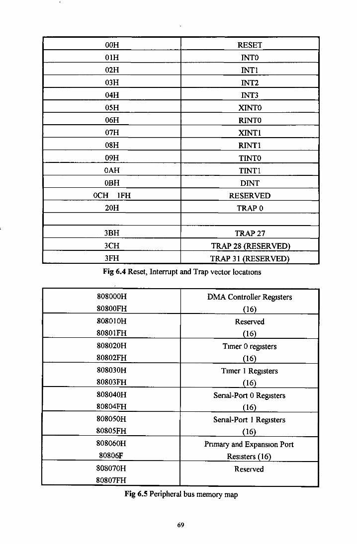
00H RESET01H INTO02H INTI03H INT204H INT305H XINTO06H RINTO07H XINT108H RINT109H TINTOOAH TINT1OBH DINT

OCH 1FH RESERVED20H TRAP 0

3BH TRAP 273CH TRAP 28 (RESERVED)3FH TRAP 31 (RESERVED)Fig 6.4 Reset, Interrupt and Trap vector locations

808000H D M A Controller Registers80800FH (16)80801OH Reserved80801FH (16)808020H Timer 0 registers80802FH (16)80803OH Timer 1 Registers80803FH (16)808040H Senal-Port 0 Registers80804FH (16)808050H Senal-Port 1 Registers80805FH (16)808060H Pnmary and Expansion Port80806F Resisters (16)808070H Reserved80807FH

Fig 6.5 Peripheral bus memory map

69

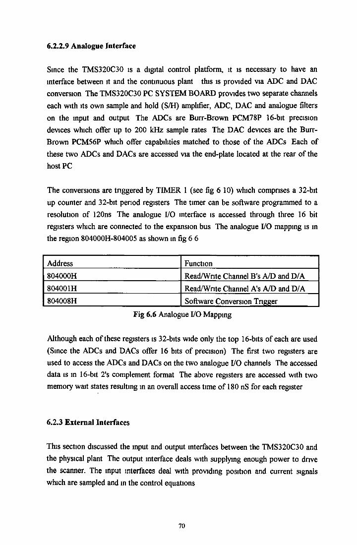
6.2.2.9 Analogue Interface

Since the TMS320C30 is a digital control platform, it is necessary to have an interface between it and the continuous plant this is provided via ADC and DAC conversion The TMS320C30 PC SYSTEM BOARD provides two separate channels each with its own sample and hold (S/H) amplifier, ADC, DAC and analogue filters on the input and output The ADCs are Burr-Brown PCM78P 16-bit precision devices which offer up to 200 kHz sample rates The DAC devices are the Burr- Brown PCM56P which offer capabilities matched to those of the ADCs Each of these two ADCs and DACs are accessed via the end-plate located at the rear of the host PC

The conversions are triggered by TIMER 1 (see fig 6 10) which comprises a 32-bit up counter and 32-bit period registers The timer can be software programmed to a resolution of 120ns The analogue I/O interface is accessed through three 16 bit registers which are connected to the expansion bus The analogue I/O mapping is in the region 804000H-804005 as shown in fig 6 6

Address Function804000H Read/Write Channel B's A/D and D/A804001H Read/Write Channel A's A/D and D/A804008H Software Conversion Trigger

Fig 6.6 Analogue I/O Mapping

Although each of these registers is 32-bits wide only the top 16-bits of each are used (Since the ADCs and DACs offer 16 bits of precision) The first two registers are used to access the ADCs and DACs on the two analogue I/O channels The accessed data is in 16-bit 2's complement format The above registers are accessed with two memory wait states resulting in an overall access time of 180 nS for each register

6.2.3 External Interfaces

This section discussed the input and output interfaces between the TMS320C30 and the physical plant The output interface deals with supplying enough power to drive the scanner. The input interfaces deal with providing position and current signals which are sampled and in the control equations

70

6.2.3.1 Output interface

To move the scanner through a desired angle, a D C voltage is used to drive current into the scanner coils The maximum required current for this scanner is approximately 1 A so it is obvious that power amplification is required To provide this amplification a unity gam Pentawatt LI65V power amplifier was selected This can provide up to 20 Watts of power (see Appendix B 2 for schematic of output interface )

6.2.3.2 Input interfaces

1. Capacitive position sensor

As can be seen from fig 6 2, two input interfaces are used depending on whether one is running the scanner under ordinary (i e with the position sensor) or sensorless control The direct position sensor is a capacitive sensing transducer whereby a stationary metal ring forms four electrodes around the grounded rotor The electrodes are configured so that each pair of diametrically opposite electrodes forms a capacitor with the rotor Each electrode pair is driven by a high-frequency voltage source which sets up a current (32|iA/°) which is related to the capacitance between the electrodes and the rotor The direction of the resulting currents are differentially amplified such that output signal determines the direction of scan angle displacement relative to the zero reference position A schematic for this circuitry is shown in Appendix B 1

2. Current sensor

Due to the magnitude of the armature current ( Up to 1A peak), it was decided against using the usual current sensing techniques as in the above position transducer Instead it was decided to put a small sensing transducer in series with the armature coils as in fig 6 7 below The value of the resistance was selected as being 0 2Qs*, as this resistance must be small relative to the armature resistance of 2 3Qs Since the sensing resistance was quite small only small voltages could be developed across it even for quite large angle displacements To increase the SNR of the resulting signal a high specification AD625 instrumentation amplifier was used This amplified the voltage signal up to the ± 3 volt level required to achieve maximum resolution from the DSP's A/D converters

1 This resistance was taken into account in the modelling stage

71

6 3 SOFTWARE DESIGN

6.3.1 Introduction

The TMS320C30 processor with its floating point instructions and new architecture can support high-level language development Programming in C, a high-level language, has several advantages over assembly language development for DSP and control applications Firstly, the control processor is usually required to do more than just implement the control equations, assembly programs can easily become unwieldy especially with regard to software upgrading/maintenance C programs are not device specific, so it is a relatively straightforward task to transfer existing C programs to/from other systems Since the software complexity is reduced so also is the development time although assembly language does produce faster code The C programming language is a structured language which offers low-level capabilities which are often used in control applications So a good compromise between high level and assembly development is that when an application requires minimum execution time to write the time critical sections of the code in assembly functions, which are then called by a C program The advantages of high level programming resulted in the implementation of the C compiler for the TMS320C30 The C compiler uses a sophisticated optimizations pass that employs several advanced techniques for generating efficient, compact code from C source code General optimisations can be applied to any C code but TMS320C30 specific optimisations take advantage of the particular features of the TMS320C30 architecture [6-4]

6.3.2 Software Development Flow

72

The TMS320C30 is fully supported by a complete set of hardware and software development tools These tools are used to transform the original C source code into executable code suitable for the target platform The basic tools used are the optimising C compiler, an assembler, a linker and an archiver To aid m the high level language development an interface library is available to facilitate program development without having to learn about the hardware details of the transfer The library routines are used to download TMS320C30 object code onto the system board, to initiate execution of this code and to pass data between the TMS320C30 and the host PC The software development is summarised in fig 6 8 below

Fig 6.8 C based TMS320 Software Development flow

6.3.3 Numerical Conditioning

The first stage in developing real time control code is to execute the code off-line using input data taken from the simulated controller and then compare the output from the code to that of the simulation This exercise, as well as testing the actual C code, is instructive in that it allows one to analyse the numerical characteristics of the code before it is implemented on-line Initially problems were encountered regarding the numerical behaviour of the system steady state offsets were obtained between the simulated output and the C code output This was due to the ill-conditioning of

73

the system matrices1 This was remedied by transforming the system using the canonical transformation The state model is not unique and it is possible to represent the model relative to a different vector basis [6-5] (not necessarily in terms of the physical variables A similar transformation is used in section 4 5) Consider the state space system

x = Ax + Bur (6 4)y = Cx

From the above non unique property it is possible to have another state vector z such that

x = Az (6 5)

where A is an (nxn) non-singular constant matrix Under this transformation the original state model is transformed into

z = A 1 AAz + A *Bu a- c.\y = CAz

The matrix A m equation 6 5 above is chosen to transform the system into controller canonical form Using this technique systems numerical conditioning, (the ratio of the smallest to the largest number), was improved from 1 Ole-6 to 0 60142 This improvement in numerical conditioning eliminated any steady state offsets introduced by the C code and gave the same output results as those obtained from the simulation

6.3.4 Software Description

The software is written in C and executes under the Spectron Microsystems SPOX system kernel (SPOX/DOS VI 3) This kemal provides access to real-time I/O and communication facilities At run time the user can specify controller/estimator gains as well as a desired position reference or choose a certain scanning action with the associated amplitude and frequency The data of interest i e position, velocity, error

1 The SIMULINK CAD package automatically compensates for ill-conditioning by appropriate scaling of the internal variables2 The system matrices are well conditioned if the conditioning is near 1, and badly conditioned if it is near 0 0

74

and control input and integrator output can then be displayed on screen or re-routed to a file, an alternative method of data capture is discussed later The program is interrupt driven and executes in real time at the sampling frequency of 6 kHz with provisions for high speed data capture

1. Timer setup

The TMS320C30 provides two general purpose timer modules which have 32-bit timer/event counters which can be signalled by either internal or external clocking (fig 6 9) The TMS320C30 system uses TIMER1 to signal the A/D converter to start a conversion Three memory-mapped registers are used by each timer, these are the global control register, the penod register and the counter register The timer global control register is a 32-bit register which contains the global and port control bits for the timer module, the first four bits (3-0) are the port control bits and bits 11-6 are the timer global control bits, the remaining bits are reserved The counter and period registers are 32-bit registers which are used to control the frequency of the timer signalling The timer counter register is reset to zero when it increments to the value of the period register, both are set to 0 at reset The memory map of the TIMER 1 locations are shown in fig 6 10 [6-3]

Internal Clock/2

Timer Out

Fig 6.10 Timer Block Diagram

75

The three registers, global-control, period and counter are memory mapped to locations 808030H, 808034H and 808038H respectively. The timer signalling rate is determined by the frequency of the timer input clock and the period register, the sample period is given by

Sample period = Value of period register x 120 (ns).

2. Interrupt Control

The TMS320C30 can respond to both internal and external interrupts. This application responds to an 'end of conversion' interrupt which halts the house keeping tasks and immediately services the controller subroutine therefore guaranteeing a 6kHz execution time in a real time1 environment (provided enough time is available to service the interrupt routine before the next interrupt occurs). External interrupts are synchronised internally using the three flip-flops clocked by HI and H3, the interrupt functional diagram is shown below. When synchronised the interrupt will set the corresponding interrupt flag register (IF) bit if the interrupt is active.

INTn

PH1

D Q

CLK

H2

Internal Interrupt set signal

D Q

CLK

D Q

CLKn

Internal Interrupt Clear/Acknovriedge

signal

EINTn(CPU)

GIE(CPU)

To Control Section

Set Q

Reset

r ^ H

Internal Interrupt Processor

GIE(DMA)

EINTn(DMA)

Fig 6.11 Interrupt Functional Diagram

3. Serial Communication

Because of the high speed 'real-time' nature of the controller, obtaining data about the state of the plant from a scrolling screen is inadequate. The TMS320C30 has two independent, bi-directional serial ports which can transfer 8, 16, 24, or 32 bits of data

1 A real-time system is a system that must satisfy explicit (bounded) response-time constraints or risk severe consequences including failure. [6-6]

76

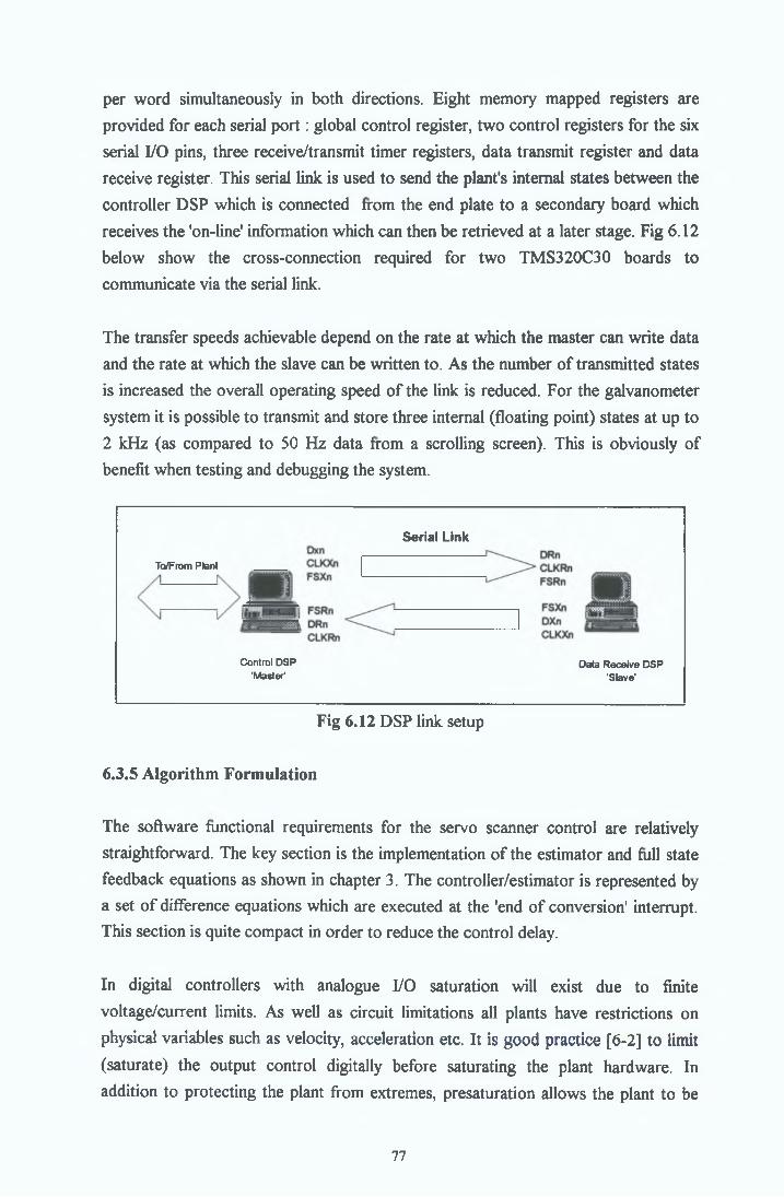
per word simultaneously in both directions. Eight memory mapped registers are provided for each serial p o r t: global control register, two control registers for the six serial I/O pins, three receive/transmit timer registers, data transmit register and data receive register. This serial link is used to send the plant's internal states between the controller DSP which is connected from the end plate to a secondary board which receives the 'on-line' information which can then be retrieved at a later stage. Fig 6.12 below show the cross-connection required for two TMS320C30 boards to communicate via the serial link.

The transfer speeds achievable depend on the rate at which the master can write data and the rate at which the slave can be written to. As the number of transmitted states is increased the overall operating speed of the link is reduced. For the galvanometer system it is possible to transmit and store three internal (floating point) states at up to 2 kHz (as compared to 50 Hz data from a scrolling screen). This is obviously of benefit when testing and debugging the system.

To/From Plant

Serial Link

Control DSP 'Master1

Data Receive DSP 'Slave'

Fig 6.12 DSP link setup

6.3.5 Algorithm Formulation

The software functional requirements for the servo scanner control are relatively straightforward. The key section is the implementation of the estimator and full state feedback equations as shown in chapter 3. The controller/estimator is represented by a set o f difference equations which are executed at the 'end of conversion' interrupt. This section is quite compact in order to reduce the control delay.

In digital controllers with analogue I/O saturation will exist due to finite voltage/current limits. As well as circuit limitations all plants have restrictions on physical variables such as velocity, acceleration etc. It is good practice [6-2] to limit (saturate) the output control digitally before saturating the plant hardware. In addition to protecting the plant from extremes, presaturation allows the plant to be

77

predictably controlled by using the presaturation control levels as input to the estimation routines This prohibits the controller from 'winding up' (having very large internal control values) when saturation occurs, this is particularly important when integral control is employed

The algorithm flow diagram is shown in fig 6 13 below and a listing of the C source code is given in Appendix C

Yes

Fig 6.13 Program Flow Chart

6 4 SYSTEM INTEGRATION

6.4.1 Input/Output Scaling

Before the system could be implemented scaling of the physical quantities was performed in order to achieve maximum resolution from the systems ADCs and DACs and to avoid saturation The ADCs and DACs are ± 3V devices where an input of 3 V is represented by a floating point number 1 0

78

6.4.2 Calibration of Sensor

The capacitive sensor, whose specifications are given in appendix was calibrated using the HEIDENHAIN 426b 12-bit encoder The encoder position information is interpolated by a further 2-bits giving an overall 14-bit accuracy The output of the encoder was mapped into the high speed TMS320C30 DSP data link, allowing calibration of the capacitive sensor output versus the encoder output The encoder was connected to the shaft of the scanner by a light-weight aluminium coupling device The scanner was made to deflect using a 2Hz sine wave (as recommended by General Scanning [6-7]) giving a quasi-static test The results of the calibration are shown in fig 6 14 below giving output position data of the capacitive sensor Vs that of the encoder

Quasi-Static Calibration of Sensor

No Samples

... Capacitive Sensor Output Encoder Output

Fig 6.14 Calibration of Capacitive Sensor

6 5 TEST AND EVALUATION

6.5.1 Introduction

In the previous paragraphs the experimental hardware and software development were shown in detail The testing of the designed galvanometer scanning system is presented in this section To test the system performance a series of real-time

79

measurements are taken, these measurements show that a high performance positioning controller mechanism is realised The results also show the validity of the sensorless control approach which has applications in fault tolerant designs, not only keeping the system within safe operating limits but also allowing it to perform with almost full functionality

6.5.2 Experimental Procedure

The experimental rig as shown in block diagram 6 2 was constructed The control software was compiled and linked using the optimising C compiler which produces the required executable file A special interface handling program called 'execlsLexe' is executed on the host P C This program downloads the executable C code onto the target platform 1 e the TMS320C30, as well as controlling the data flow between the host P C and the board The user can specify the control/estimator gains by supplying the required command line arguments A typical command line might be

execlsi SCAN.X30 /pi /vl /cl /il /PO 1[PC program] [Control program] [Command line arguments]

Which tells the system to execute the program SCANX30 on the TMS320C30 target board, it specifies position, velocity, current and integral gains of 1 and a desired position reference of 0 1 rads

The controller begins execution and actuates the galvanometer through the required dynamics to the desired position The data associated with this motion is sent in real time to a secondary 'slave' TMS320C30 board via a senal-link as discussed above This data is stored temporarily in high-speed R A M and later written to disk for processing This data is then directly loaded into the MATLAB CAD package for examination

6.5.3 Performance Using The Position Sensor

This section deals with the performance of the controller when using the capacitive position sensor The tests are designed to see how well the control system can track a position reference signal and changes in this signal This is done by subjecting the test ng to stepping, ramping and sinusoidal position commands and examining the systems response to these commands

80

6.5.3.1 Test with ITAE design

The ITAE design uses a performance index as described in section 5 2 2, the controller was designed using root locations specified by the ITAE 'optimum form' template for a fourth order system The response for this design during a scanning action is shown in fig 6 15 below The response has an overshoot of approximately 20% and a settling time of 4 1 ms

6.5.3.2 Test with L Q R design

The discrete LQR design uses a feedback gain that minimises a cost function based on a weighted linear combination of the system state and input variables The detailed design of the LQR based controller is given in section 5 2 4 The actual results obtained from the ng using this controller implemented in real time are shown in fig 6 15 below The results show an overshoot of approximately 11% and a settling time of 2 9ms

Both designs meet the requirements in that the resultant controller has a fast dynamic response and has zero-steady state error to a reference position signal However it is obvious that the LQR based design has a better overall response in terms of settling time and overshoot, therefore it is the LQR based controller which is the preferred controller type The results obtained confirmed the simulation results which suggested that the LQR design gave better response for this application The step responses using both controllers are shown below for comparison purposes1 The response of the LQR to sinusoidal, ramp and step input commands are shown in figs 6 16-6 19

1 The resolution in the plots shown here is less than the system resolution because the serial link between the master and slave DSP boards operates m real time at 2kHz compared to the plant which is run at 6kHz

81

Actual Response of ITAE based controller1 ---- --------- ■ ............. . -----------------------

\tf

I

S»

fr

/

0 0 005 0 01 0 015 0 02 0 025Time ms

, ________________ Actual Response of LQR based controller_________ ________________

- .................. - ..........................

----

----

--1--

------

------

-----

i I i i i I i i » i i I i i i l i ....... ._____________________

///ir

1Jt

/y

0 0 005 0 01 0 015 0 02 0 025Time ms

Fig 6.15 Comparison of ITAE and LQR design responses

The results obtained from the ng are compared to the results taken from the simulations in fig 6 20 They show a good correspondence in terms of rise time and settling time Although the actual results obtained have a slightly greater overshoot then the simulated response the overall dynamic behaviour is satisfactory and matches up well with the simulated responses showing no steady state error to a position command

82

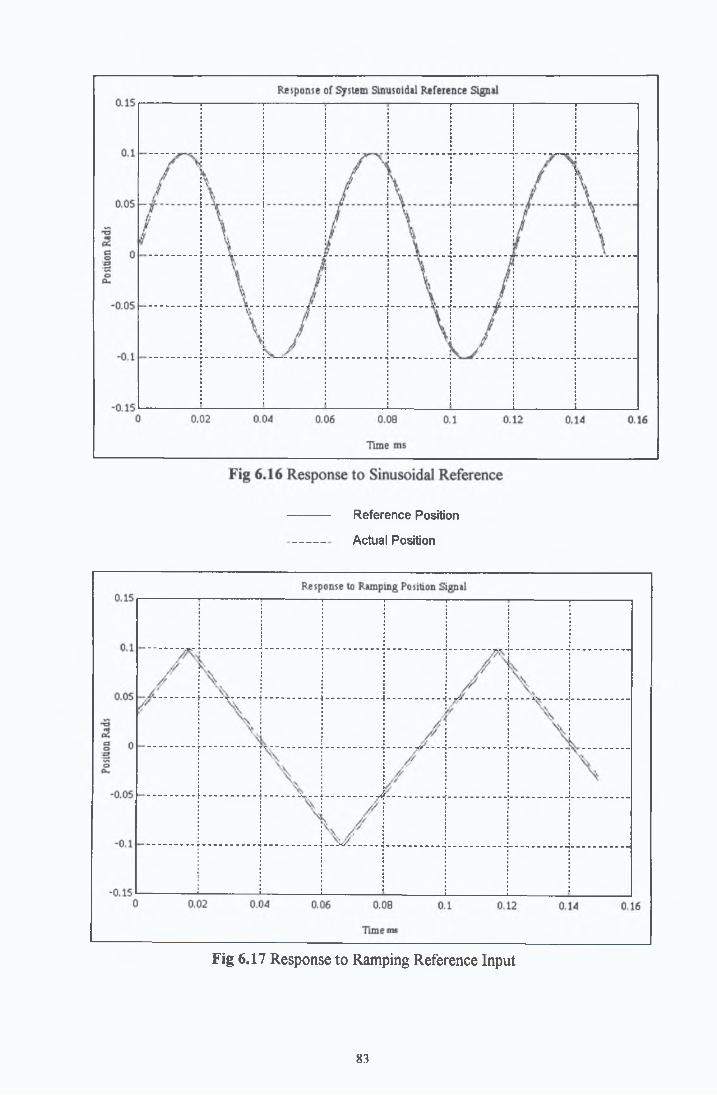
Reference Position

Actual Position

Fig 6.17 Response to Ramping Reference Input

83

Posit

ion

Rads

I

Posit

ion

Rads

Response to Step Input Reference

Time ms

Fig 6.19 Response to Step Input Commands

Fig 6.20 Actual Position(—) Vs. Simulated Position( ••)

84

6.5.4 Performance Using the Sensorless Control Approach

Section 5 6 presents the use of sensorless control for voice coil motor applications It suggested that it is possible to control the motion of the galvanometer scanner without using any direct position/velocity transducer This is to be achieved by utilising the known information of the system via a system model in conjunction with measurements of the easily accessible terminal quantities, i e voltage and current This information is used in a Kalman algorithm to estimate the unknown quantities of position and velocity

The sensorless control strategy was successfully implemented on the galvanometer scanner As explained earlier the actual position as sensed by the capacitive sensor is measured for comparison purposes to validate the approach and is not used in the controller equations The sensorless control method was tested as in the previous section with the results in fig 6 21 and fig 6 22 below showing the system following desired commands without using any direct sensor

S e n s o r le s s C o n tro l W ith S te p In p u t

N o S a m p le s a t 6 k H z

Fig 6.21 Response of sensorless control to step input command

85

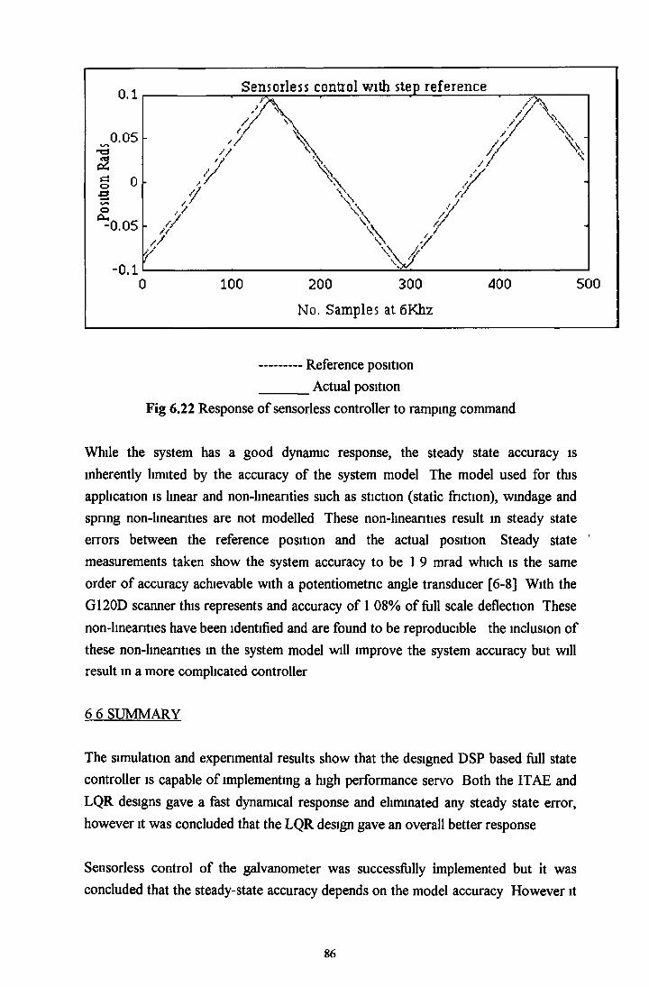
Reference position______ Actual position

Fig 6.22 Response of sensorless controller to ramping command

While the system has a good dynamic response, the steady state accuracy is inherently limited by the accuracy of the system model The model used for this application is linear and non-linearities such as stiction (static friction), windage and spring non-lineanties are not modelled These non-lineanties result in steady state errors between the reference position and the actual position Steady state J measurements taken show the system accuracy to be 19 mrad which is the same order of accuracy achievable with a potentiometnc angle transducer [6-8] With the G120D scanner this represents and accuracy of 1 08% of full scale deflection These non-linearities have been identified and are found to be reproducible the inclusion of these non-lineanties in the system model will improve the system accuracy but will result in a more complicated controller

6 6 S U M M A R Y

The simulation and experimental results show that the designed DSP based full state controller is capable of implementing a high performance servo Both the ITAE and LQR designs gave a fast dynamical response and eliminated any steady state error, however it was concluded that the LQR design gave an overall better response

Sensorless control of the galvanometer was successfully implemented but it was concluded that the steady-state accuracy depends on the model accuracy However it

86

is clear that this type of control has applications in lower specification systems or possibly in fault tolerant designs which in the case of sensor failure can not only keep the scanner within safe operational limits (which is obviously important when high performance lasers are being deflected) but can give the scanner almost full functionality

87

CHAPTER 7

CONCLUSIONS AND RECOMMENDATIONS

7.1 Summary and Conclusions

This thesis outlines a methodology for the design of a discrete controller applicable to voice coil actuators A specific voice coil actuator i e the galvanometer scanner, is chosen as a target application for the design The design process presented is based on the following phases

• System Description• Control Approach• System Identification• Control Design• Implementation

The research focused on the design of a digital position controller for a commercially available galvanometer scanner using modem full state feedback techniques The initial emphasis was to develop a mathematical model of the plant, this step was not only beneficial in terms controller design and simulation but also provided an insight into the systems dynamic and steady state behaviour as well as its stability and performance limitations

The control approach was then discussed resulting in the selection of a full state feedback controller/estimator topology as discussed in chapter 3 The controller design phase was presented where two methods were used in selecting the systems closed loop root locations, these locations directly reflect the dynamic and steady state characteristics of the controller

The first method used the ITAE criterion which is based on a standard template defined in terms of the order of the closed loop system The second design method was done using the modem LQR design, whereby a weighting is attributed to the systems internal states and to the input control, relative to their respective importance's The system design was simulated in both continuous and discrete time, the overall objective being to develop a satisfactory discrete design

88

The estimator design was examined where it was shown that the systems unmeasured states could be reconstructed using certain mput-output data and the system model This estimation process was expanded and the elimination of the systems direct position sensor was considered, this led to the term 'Sensor less' control

The implementations were performed with both the ITAE and LQR designs The experimental data concurred with the simulated data and it was concluded that the LQR design gave the better over all response although both designs worked well in having fast dynamic responses and zero steady state errors

The discrete control design was implemented both under conventional control 1 e using a position sensor and under sensorless control with experimental results presented for each case confirming the performance of high speed control and also the validity of sensorless control The sensorless control is of special interest and may have some important applications within the voice coil actuator based industries (See below)

7.2 Recommendations

7.2.1 Within the Voice Coil Actuator Industry

7.2.1.1 Cheaper Designs

The work presented in this thesis illustrated how modem control methods can be applied to voice coil actuator control Sensor-less control was implemented and was found to perform in a satisfactory manner although with limited accuracy In lower specification applications the implementation of the sensorless control technique wouls reduce the scanner in terms of manufacture (simpler design) and sensor purchases (no sensor required)

7.2.1.2 Fault Tolerant Designs

The sensorless control scheme could also be used in high end applications such as space communications and military night vision systems In these applications m the event of sensor failure the sensorless design would assume control and would not only keep the system within safe operational limits but would also allow it to perform with almost full functionality

■>89

7.2.1.3 Operation with other Voice Coil Actuator based systems

In modem disk drives the position of the read/wnte head is written on the disk at the time of manufacture The controller then reads this position information and performs a stepping action to the next position reference Using the sensorless approach a position requirement is transferred into an alternative requirement 1 e an input voltage or current this requirement is first achieved directly without reading any of the position information moving the read/wnte head to within a certain range of the desired position The convention more accurate (and slower) controller would then assume control finally driving the position error to zero Therefore the sensorless approach may well have applications within the computer disk drive industry

7.2.2 For further research

As was stated accuracy achievable with the sensorless approach was limited to the accuracy of the system model Unmodelled non-lineanties due to stiction and spring imbalance manifest themselves as steady state errors, the accuracy achievable may therefore be increased by the inclusion of these non-lineanties in the system model [7-1]

The control algorithms developed here may be developed further by the inclusion of self-tuning-adaptive control

90

References

CHAPTER 1

1-1 J Stupak, G Gogue, "Voice-Coil Actuators Insight into the design", Proceedings of the 16th International Intellgient Motion Conference pp 241-53, 1986

1-2 G Franklin, J Powell, M Workman "Digital Control of Dynamic Systems",2nd E d , Addison-Wesley, 1990

1-2 "Laser Applications", Vol 2 , Academic Press, 1974 ' ,

CHAPTER 2

2-1 "YAG 100-300 series laser specifications", ADLAS ltd, Stow M A

2-2 "Melles-gnot, Optics Guide 3", 1985

2-3 "Laser Beam Scanning, Opto-mechamcal devices, systems and data storage optics", Marcel Dekker Inc, Newyork 1985

2-4 Galvanometer Scanner Users manual, General Scanning Inc, Waterton MA, 1988

2-5 W Brogan, "Modern Control Theory", 3rd Ed, Prentice Hall, 1991

2-6 A Bukys,"Beam Deflection and Scanning Technologies", SPIE Vol 1454 1991

2-7 "Laser Applications", Vol 2, Academic Press, 1974

CHAPTER 3

3-1 C J Maday "CAD design of feedback control systems",Research Triangle Park 1987

3-2 IJ Nagrath, M Gopal, "Control Systems Engineering", 2nd Ed ,Wiley & Sons 1982

3-3 H Anton, "Elementary Linear Algebra",5th Ed, Wiley & Sons 1987

3-4 "MATLAB reference guide", Mathworks Inc, 1992

3-5 W Brogan, "Modem Control Theory", 3rd Ed, Prentice Hall, 1991

3-6 G Franklin, J Franklin, M Workman, "Digital Control of Dynamic Systems",2nd Ed, Addison-Wesley 1990

CHAPTER 4

4-1 "Identification Toolbox Users Guide", Mathworks Inc, 1991

4-2 L Ljung "System Identification, Theory for the User", Prentice Hall, 1987

4-3 S Haykin," Communications Systems", 2nd Ed, Wiley and Sons, 1983

4-4 I Landau," System Identification and Control Design", Prentice-Hall, 1990

4-5 P Wellstead, M Zarrop,"Self-Tuning Systems, Control and Signal Processing", Wiley and Sons, 1991

CHAPTER 5

5-1 G Franklin, J Powell, M Workman, "Digital Control of Dynamic Systems", 2nd Ed, Addison-Wesley, 1990

5-2 IJ Nagrath, M Gopal, "Control Systems Engineering", 2nd Ed ,Wiley & Sons 1982

5-3 "Control Systems Toolbox Users Guide", Mathworks Inc, 1991

5-4 G Thomas, R Finney, "Calculus and Analytic Geometry", 6th Ed, Addison- Wesley 1986

5-5 A Bryson, Y Ho, "Applied Optimal Control", Halstead Press, 1975

5-6 J. Barnes, "Electronic System Design, Interference and Noise Control Techniques", Prentice-Hall, 1987.

5-7 R. Brown, "Introduction to random signal analysis and Kalman filtering", Wiley 1983.

5-8 D.E. Catlin, "Estimation, Control and the Discrete Kalman Filter". Springer-

Verlag, 1989.

5-9 B. Rohr, "Speed Vs. Accuracy in galvo-based scanners", Laser & Optronics,pp 15- 18 vol 11(2), !992.

5-10 N. Mohan, R. Dhaouadi, "DSP-based control of a PMSM with estimated speed and rotor position", EPE '91 proceedings, vol 1 pp 596-602.

CHAPTER 6

6-1 P.E. Papamichalas, "DSP applications with the TMS320C30 family", Prentice- Hall, 1990

6-2 G. Franklin, J. Powell, M. Workman, "Digital Control of Dynamic Systems", 2nd Ed., Addison-Wesley, 1990.

6-3 "TMS320C30 Users's guide DSP products", Texas Instruments Ins., 1991.

6-4 "TMS320C30 Optimising C Compiler Reference Guide", Texas Instruments Inc., 1990.

6-5 G. T.R. Finney, "Calculus and Analytic Geometry",6th Ed., Addison-Wesley 1986.

6-6 P.A. Laplante, "Real-Time System Design and Analysis : An Engineers Handbook", IEEE Press, 1993.

6-7 "Galvanometer Scann Users manua", General Scanning Inc., Waterton MA, 1988.

6-8 B. Rohr, "Speed Vs. Accuracy in galvo-based scanners", Laser & Optronics, ppl5- 18 vol 11(2), 1992.

93

CHAPTER 7

7-1 H Hennchfreise, "Observer-based Coulomb friction torque compensation for a position control system", Intelligent Motion Proceedings April 1992, pp 82-92

94

Appendix A.1

SIMULATION

Idsim Simulate a general linear system

mkthetha Create a theta-format model

PARAMETER ESTIMATION

ar Estimate AR modelarmax Estimate ARMAX modelarx Estimate ARX modelusing least squaresbj Estimate Box-Jenkins modeldtrend Remove zero'th and first order trendsIV Estimate ARX model using IV-methodivar Estimate AR model using IV-methodIVX Estimate ARX model using general instrumentsiv4 Estimate ARX model using four stage IV-methodoe Estimate output error modelpem Estimate general linear model

NONPARAMETRIC ESTIMATION

covf Estimate covanance functionetfe Estimate transfer functions using

direct Founer techniquesspa Estimate spectra and transfer functions

using spectral analysis

MODEL CONVERSIONS

contin Theta to continuous-time modelpolyform Theta to transfer function polynomialstrf Theta to frequency functions and spectratrfcont Theta to frequency functions for

corresponding continuous-time modelszp Theta to zeros, poles and static gains

MODEL PRESENTATION

bodeplot Plot bode diagramsidplot Display input-output datapresent Display model on screenzpplot Plot zeros and poles

I

Appendix A.2

Continuous system Discrete system

0 0 I 0(k) 0(k+1) l(k)

transform

M

Canonical representation

0(k)0(k+1)0(k+1)

discretisation

Discrete system

0(k) 0(k+1 ) l(k)

Canonical representaton

¡gl M'1«pii 0(k) 0(k+1) 0(k+1)

Heuristic transform

System Identification

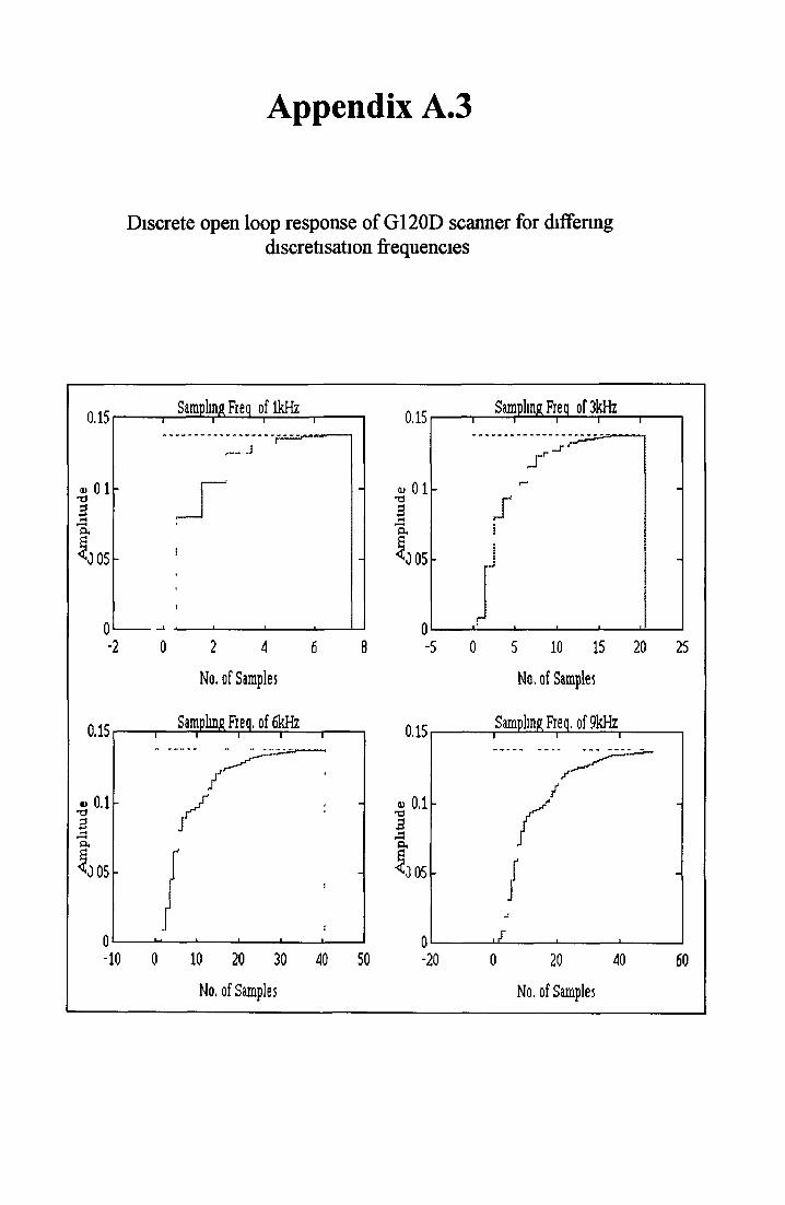
Appendix A.3

Discrete open loop response of G120D scanner for differing discretisation frequencies

Appendix B

Interface Circuitry

Appendix B .l Input Interface Circuitry

The input interface circuitry differentially amplifies two input current signals which are generated by the G120D capacitive position sensor. The magnitudes of the current signals are proportional to the scanner rotation angle and the signs of the signals are dependant on scanner direction.

From the diagram using the basic op-amp equations for the first stage we have

II + 12 + 13 = 0 Vo - VI

II +VI

= 0RI R2

Vo = -I1R1 + V l(l + r ^ 2)

and for the second amplifier it is clear that:

R1 R1 R2By substituting in with Vo above and using II = -12=> I2R1 + I2R1 + VI Rj £ 2 + Vo’ -VI’ ̂ YK1 = 0By equating and cancelling we get Vo'= 2*12

This position signal is further amplified to provide the necessary signal levels When building this circuit grounding considerations are very important and current ground loops/losses must be avoided, see reference 5-6 for further details

Appendix B.2 Output Interface Circuitry

The output circuitry acts as the driver from the low power D/A output It supplies the current which is driven into the coils of the voice coil actuator The LI65V power amplifier is rated for 3 2 Amps at 20 Watts

Appendix B.3 Current Sensing Circuitry

This circuitry is used when the galvanometer is operating under the 'sensorless' control mode It is comprised of a small sensing resistor in series with the motor windings and the AD625 instrumentation amplifier When a current passes through the motor windings a small voltage, proportional to the motor current, is dropped across the sensing resistor This voltage is differentially amplified resulting in a significant increase in SNR, it also makes use of the ±3V input range used on the TMS320C30 thereby increasing the measurement resolution

The schematic diagrams for the three interfaces are shown below

J . JEMBft

T i t u

8 * n s o r I n t« r f a o « C i r c u i t r y

8 ÌM

Â

D o ouM ot R uabas MEV

1 /1

D «t« i Au o u s t 2 € . 1994 I s b M t 1 o f 1

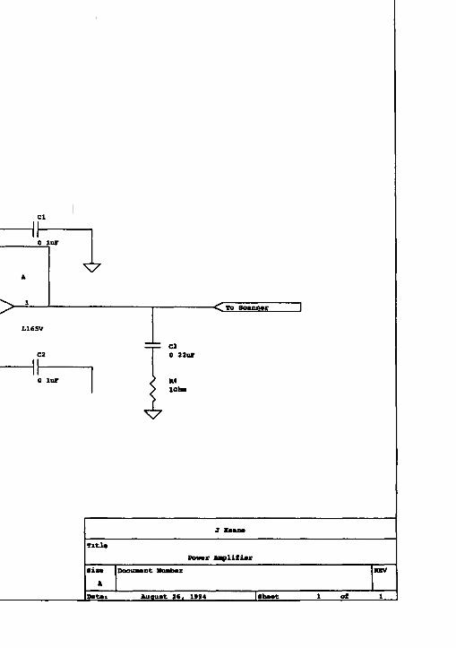
Cl

J Emmam

T x tl»

P o v v r A B p l i f i * r

l i s * DoouaMQt Buab*x REV

A

P at«» JU iq u it 2 6 , 1 IM l<h— t 1 o f 1

^ I m/oat ^R1

lk

8*nsingJ t o s i e t o r

R60 2 Ohm

< I In/OutT1 k

vccQ

16 - I / P

15 - a m d m

12 —Q 8«DM

5 +<S S anaa

2 +Q 6«DM

AD625IX

output

■C To Qgg i

•fl/p

J X aana

T i t l a

C u r r a n t S a n a in g C o t

8 iM

A

D oooaan t l a b a r

3

u v

P a t t i t o q a i t > , 1M4 |g h —t 1 o f \

Appendix C

Generic C source file listing

J* *//* This listing presents the core of the galvanometer control software The changes between *//* this core listing and other application dependant variants are highlighted where relevant *//* *//* John Keane 9-4-1994 *//* *//I************************************************************************/

/* TMS320C30 specific libraries */

#mclude "dsp hnk h"#include "std_lib h"

#mclude<stdio h>#mclude<math h>#include<stdlib h>

#deflne IRINT01 0x2

#define OFF 0 #define ON 1

#define DISPLAY 5 #define CON 6

#define FREQUENCY 6000Mefine CONTROLFREQ 6000

#define T (double) 1/FREQUENCYMefine BITS 256

Mefine Pscale 0 17453

Mefine pause() getchar(),#defme saturate(a,b) ((a)>(b))^(b) ((a)<-(b))^(-b) (a),

void Imt_ISR(unsigned int), void c_int01(void), void setvectO, int getvect(int num),

I* Scrolls internal states to screen *1

extern displayO,

void GIE(int),

1

double A[3][3]={{ 87604617,0 0,0 0),{0,0 65042209,0 5517210},{0,-0 5517210,0 65042209}>,

double B[3]={-14 2661917,0 8083793,75 2218214},

double C[3]= {-0 00125935197,0 000066861893,-0 0002211871},

double D=0 0,

double L[3]={0 7,2367 2,1 4},

double M[3][3]={{-0 00125935,0 000066861893,-0 0002211871},{0 9999892,0 86980642,0 4933913},{-0 00446441,-0 0009227382,0 0009384}},

double X_[3]={0,0,0},

double Xbar[3]={0,0,0}, double Xhatt3]={0,0,0},

double Xepos=0 0,

int echo=DISPLAY,

double pos=0 0,vel=0 0,curr=0 0,possc=0 0,Preft=0 0,Eput=0 0,

double Pref=0 0,input=0 0,posmeas=0 0,epos=0 0,posref=0 0,intout=0 0,Perror=0 0,

double Kp=13 159,Kv=0 00272,Kc=l 902,Ki=25232,

double Ein=0 0,e=0 0,Eout=0 0,

char command[256],

char *ptr,

int IN_ISR=0,

unsigned long real_timer=0,

smain(mt argc,char *argv[]){mt i,double vtmp=0 0,ptmp=0 0,

/* Inputting controller and estimator gams */

for(i= 1 ,i<argc,i++){if(*(aigv[i]++)=T){

switch(*(argv[i]++)){ case T' Pref=ptmp=atof(argv [1]), pnntfCPosition %f\n",Pref),

break,case 'p' Kp=atof(argv[i]),

break, case V Kv=atof(argv[i]),

break, case 'c' Kc=atof(argv[i]),

break, case V Ki=atof(argv[i]),

break,case 'L' L[0]=atof(argv[i++]),

L[l]=atof(argv[i++]),L[2]=atof(argv[i]),break,

case 'E'break,

case 'C echo=CON, break,

}}

>

Iiut_ISR(FREQUENCY),

pnntf(”\033[2J"), /*clrscr*/

while(l){display_main(),

/* When using the high speed DSP link for test purposes */ /* the code is executed here */

}

}

/* Initialising the interrupt vectors */

void Imt_ISR(unsigned int freq){int * temp, temp=PRIMCTL,1"temp=0x800,temp=EXPCTL,*temp=0x00,setvect(IR_INTO 1 ,c_intO 1), set_timer(f5req), enable(IR_INTO 1),}

void c_int01(){real_timer++,

Ein=(double)in_channel(A_CHAN)/32768,posmeas=(double)in_channel(B_CHAN)/32768,Ein=Ein*3 0, controller(posmeas),outport(A_CHAN,(double)(Eput)*32768),

return,>

void controller(double posm){/* When following certain profiles for example a Ramping scan, the position */ /* reference generation code is placed here */

Xbar[0]=A[0] [0] *Xhat[0]+B[0] *Ein, Xbar[l]=A[l][l]*Xhat[l]+A[l][2]*Xhat[2]+B[l]*Ein,Xbar [2]=A[2] [ 1 ] *Xhat[ 1 ]+A[2] [2] *Xhat[2]+B [2] *Ein,

posmeas=posmeas*Pscale,

epos=posmeas-pos,

Xhat[0]=Xbar[0]+L[0] *epos,Xhat[l]=Xbar[l]+L[l]*epos,Xhat[2]=Xbar[2]+L[2] *epos,

pos=C[0]*Xhat[0]+C[l]*Xhat[l]+C[2]*Xhat[2], vel=M[l][0]*Xhat[0]+M[l][l]*Xhat[l]+M[l][2]*Xhat[2], curr=M[2] [0] *Xhat[0]+M[2] [ 1 ] *Xhat[l]+M[2] [2] *Xhat|2],

Perror=Pref-pos,

intout=intout+Perror*T,

Eout=intout*Ki-Kp*pos-Kv*vel-Kc*curr,

Pref=saturate(Pref,0 1745),

Eout=saturate(Eout,l 7), /♦Set max out voltage to 1 5 mitally */ Eput=(-Eout/3 0),

return,>

display_mam(){double tmp, char c,if(echo=DISPLAY) displayO,

if(echo=CON){pnntf("Command>>"),gets(command),ptr=command,switch(*ptr)

{case 'A' Pref=atof(-H-ptr),

break,case T)' echo=DISPLAY,

break,case 'p' Kp=atof(-H-ptr),

break,case V Kv=atof(++ptr),

break,case Y Ki=atof(++ptr),

break,case 'c' Kc=atof(++ptr),

break,case 'L' switch(*(++ptr))

{++ptr, /*=*/

case '1' L[0]=atof(++ptr),break,

case '2' L[l]=atof(++ptr),break,

case '3' L[2]=atof(++ptr),break,

>break,

case'?' pnntf("\033[H\033[J"),pnntf("Kc=%f Kp=%f Ki=%f Pref=%f Vref=%f \nL= %f %f %f\nK=%f KC=%f\n",Kc,Kv,Kp,Pref,L[0],L[l],L[2]), break,

default break,}>

}