Report on water demand and deficiency by Partner 7, CSIR South Africa

Modeling Mkomazi water demand and deficiency

The activities for both these work tasks are reported collectively for the Mkomazi due to the

integrated nature of the CSIR’s involvement in both the demand and deficiency modelling in this

catchment, compared to only deficiency modelling for the individual Mbuluzi and Mpfure

catchments. The collation of suitable input data for modelling water demand and the final

production of spatially referenced demand data for the Mkomazi were completed in close

collaboration with the partner 6 University of Natal), because of the associated overlap of

technical expertise in terms of hydrological and spatial modelling. Suitable environmental, socio-

economic and topographic datasets were sourced from a variety of organisational and published

sources. Significant inputs and assistance was received from both Umgeni Water and the

Department of Water Affairs and Forestry, who are also key potential end-users of the IWRMS

project deliverables. Digital GIS coverages that spatially represent the various demand /

deficiency scenario’s have been produced, and are available in the project database (in ArcInfo

format).

Three different approaches have been used to develop water “demand / deficiency” scenario’s for

the Mkomazi (South Africa). The primary approach has been to model stream flow and

associated demand / deficiency values for different present and future scenario’s using the ACRU

hydrological model. These results, which constitute the definitive hydrological dataset for the

catchment,are reported in Taylor et al (2000). Two alternative approaches are reported, which

were developed as simplistic, spreadsheet-based alternatives to final demand / deficiency

modelling within ACRU (although outputs from initial ACRU model runs are used as primary

inputs in some of these spreadsheet models). These two procedures are presented for

comparative purposes only. It is important to realise that in all three modelling approaches, the

same fundamental spatial frameworks have been used to ensure a degree of standardisation.

These are based on the same sub-quaternary catchment cells, and the land-use patterns

described in the South African National Land-Cover database (Thompson, 1999; Fairbanks et al,

2000).

The two alternative modelling scenario’s provide a more generalised overview of current and

future demand / deficiency conditions in the Mkomazi catchment, based on very specific sectoral

demand and abstraction parameters (not all of which are directly comparable to the primary

ACRU model outputs). The first approach uses a simple balancing-model approach, based on the

difference between ACRU simulated natural baseline (i.e. pristine vegetation conditions), and

ACRU-modelled stream flow conditions for various sector abstraction conditions. The second

approach is based on the spatial disaggregation of pre-published sector abstraction demands,

that have been spatially re-distributed on the basis of associated land-use patterns that have

been derived from a ‘standard’ land-cover database. The objective being to compare the variation

in outputs from very different modelling approaches, with different levels of both technical and

scientific complexity, but with essentially the same objectives and spatial frameworks.

Results

1 GIS data collection and modeling : Mkomazi water demand (WT 720)

1.1 Results from the ACRU-based modelling

A series of demand / deficiency scenario’s were generated using data generated within the ACRU

hydrological model. This modelling process is documented in Taylor et al (2000). What is

described below are the key ACRU derived datasets that have been used to generate the GIS

spatial coverages that illustrate specific demand / deficiency scenario’s. The following ACRU

model outputs were used :

• Baseline flow : values represent simulated, accumulated stream flow the scenario of

pristine natural conditions (i.e. Acock’s vegetation)

• Environmental demand flow : values represent simulated, accumulated stream flow

required to meet the environmental reserve requirements

• Current stream flow : values represent simulated, accumulated stream flow the scenario of

present land-use (i.e. present forestry, irrigation and dryland cultivation), with present

domestic and livestock abstractions, and potential inter-basin transfer from the Smithfield

(Phase 1) scheme, but excluding any environmental demand and SAPPI-SAICOR

abstraction.

• Future stream flow (scenario 1) : values represent simulated, accumulated stream flow the

scenario of present land-use (i.e. present forestry, irrigation and dryland cultivation), with

future domestic and livestock abstractions, potential inter-basin transfer from the Smithfield

(Phase 1) scheme, SAPPI-SAICOR abstraction, but excluding environmental demand.

• Future stream flow (scenario 2) : values represent simulated, accumulated stream flow the

scenario of modified land-use (i.e. present irrigation and dryland cultivation, but with a 10

% increase in afforestation), with future domestic and livestock abstractions, but

excluding both environmental demand, potential inter-basin transfer from the Smithfield

(Phase 1) scheme, and SAPPI-SAICOR abstraction.

• Future stream flow (scenario 3) : are the same as future scenario 2, but include potential

inter-basin transfer from the Smithfield (Phase 1) scheme, and SAPPI-SAICOR abstraction

values, but still exclude any environmental demand.

The abstraction rates for the Smithfield (Phase 1) scheme are potential only, due to the fact that

the scheme is not yet operational. So the use of the terms “current” and “present” to describe

certain stream flows, and associated demand / deficiency scenario’s is not technically correct,

since a potential demand has been integrated with actual abstractions. Where inter-basin

transfers have been included, it has been assumed that no dam releases are made for

downstream use unless the (Smithfield) dam is full.

SAPPI-SAICOR abstraction, which consititutes the primary component of the industrial sector,

have only been included in certain scenarios for comparison, due to the location of this

abstraction at the seaward mouth of the catchment (in modelling cell 52), and the negligible effect

that this position will have on upstream catchment hydrology.

All values are reported in million cubic metres (Mm3), and have been calculated for both mean

annual, mean September, and September dry conditions in order to cover both ‘normal’ and

extreme (dry) conditions. Spatial distribution patterns for land-use demand were derived from the

South African National Land-Cover database (Thompson, 1999; Fairbanks et al, 2000).

The following demand / deficiency scenarios were calculated from the ACRU-modelled stream

flow’s :

• Present total sector demand i.e. [baseline - present stream flow ] + environ. demand

• Present total stream flow deficit i.e. baseline - present total sector demand

• Future total sector demand (1) i.e. [baseline - future stream flow (1) ] + environ. demand

• Future total stream flow deficit (1) i.e. baseline – future total sector demand (1)

• Future total sector demand (3) i.e. [baseline - future stream flow (3) ] + environ. demand

• Future total stream flow deficit (3) i.e. baseline – future total sector demand (3)

• Present total demand as a % of baseline

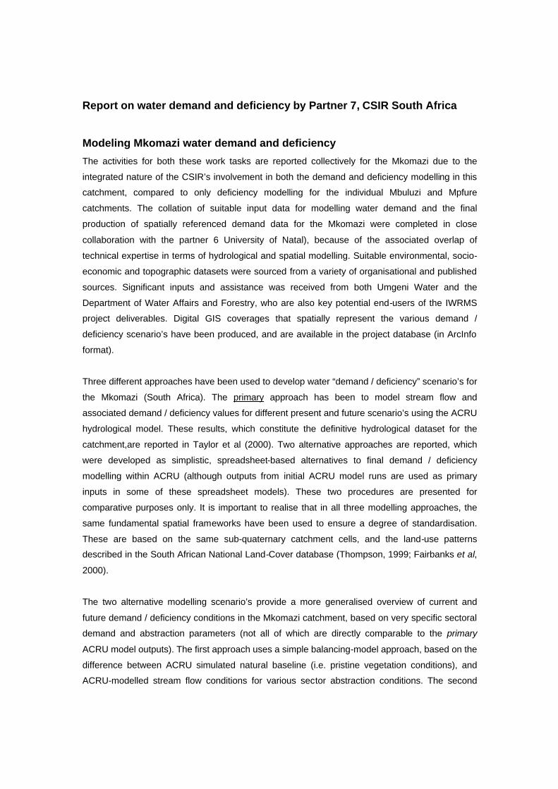
• Future total demand (1) as a % of baseline

• Future total demand (3) as a % of baseline

Actual values, and descriptions of the various sub-scenario’s are contained in the accompanying

spreadsheet “combined ACRU runoff data for Mkomazi.xls”. All are available as digital GIS

coverages, of which selected ones are illustrated below :

Present total demand (mean annual) Present total demand (Sept mean)

Future total demand (1) (mean annual) Future total demand (1) (Sept mean)

Future total demand (3) (mean annual) Future total demand (3) (Sept mean)

Future total stream flow deficit (1) Future total stream flow deficit (1)

(mean annual) (Sept mean)

Present total demand as a % of baseline Present total demand as a % of baseline

(mean annual) (Sept mean)

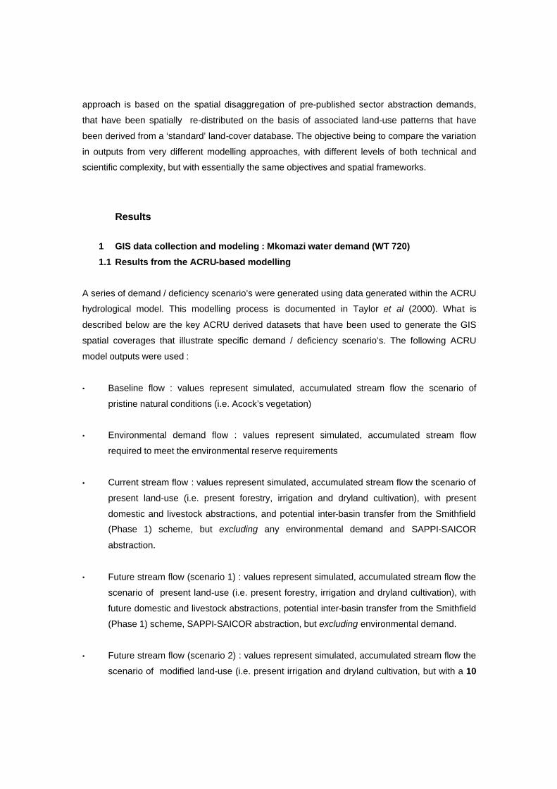
Future total demand (1) as % of baseline Future total demand (1) as % of baseline

(mean annual) (Sept mean)

Future total demand (3) as % of baseline Future total demand (3) as % of baseline

(mean annual) (Sept mean)

1.2 Results from the land-cover disaggregation framework modelling

An alternative approach to modelling water demand and deficiency was tested in the Mkomazi

catchment, based on pre-published sector demand data that was spatially disaggregated to sub-

quaternary catchment levels using land-cover distribution patterns. The objective being to

compare, if feasible, the results of a modelling routine which was based on spatially defined

hydrological principles (i.e. ACRU), to one where the same spatial resolution and thus run-off

distribution was achieved only after calculation of initial sector water demands using a different

hydrological model.

Sector demand information, i.e. livestock, irrigation, afforestation, industrial, domestic (rural and

urban) and environmental, was sourced primarily from the “DWAF / Umgeni Water : Mkomazi-

Mgeni Transfer Scheme Pre-Feasibility Study” (Ninham Shand, 1998). The reported

environmental reserve requirements were cross-checked against similar data (based on IRF’s),

reported in “Instream Flow Requirements (IFR’s) : Selected extracts of hydrological relevance

taken from IFR studies 1992-1999“ (GIBB Africa, 1999). Extraction data for the proposed

Smithfield Dam scheme was sourced from the Durban office of the Dept. Water Affairs and

Forestry, and cross-checked with Umgeni Water (Summerton pers com).

The published sector demand data was disaggregated down to the required sub-catchment level

using the land-cover distribution patterns from the 1:250,000 scale SA National Land-Cover

database (Thompson, 1999, Fairbanks et al, 2000). This was achieved in a two-step process,

whereby individual water demand sectors were linked to specific land-cover classes (or unique

class-groupings). The spatial distribution of the land-cover classes was then used to spatially

characterise the point-value demand data on a proportional basis. For example, quaternary

catchment X contains 100 ha of afforestation, distributed as 50 ha in sub-catchment X1, 20 ha in

X2 and 30 ha in X3, with a published total demand of 20,000 Mm3/a. Then the spatially

disaggregated afforestation water demand would be 10,000 Mm3/a in X1, 4000 Mm3/a in X2 and

6000 Mm3/a in X3.

The validity of this modelling approach is supported by the fact whilst there may be significant

differences between published and land-cover derived land-use areas, there are strong

similarities in distribution trends at quaternary catchment level (e.g. forestry and irrigation). This

variation is to be expected since the published datasets, are in most cases, derived from datasets

that pre-date the National Land-Cover dataset.

Due to inherent data constraints, certain assumptions were made during modelling process that

may limited direct comparability with the ACRU-derived results. This however should not be seen

as a limitation, but rather an indication of the differences that are likely to be encountered when

comparing potentially equivalent results, which have been derived from two very different

analytical procedures. For example, the (hydrological) modelling procedures used to generate the

published data may well differ from the ACRU-based approach, since the original input data used

in the published data was itself disaggregated from four basic sub-catchments. Conditional rule-

based parameters governing for example, the modification of scenario’s such as increasing

afforestation, irrigation, or the use of groundwater also differed between the two approaches.

In some cases scenario differences were also noted between the two published data sources,

necessitating assumptions that it was possible to equate ‘worst case’ scenario’s (as reported

N.Shand, 1998), with the drought-level IFR’s (as reported in GIBB Africa, 1999), in order to

“normalise” the data.

Certain modelling rules were also governed by the nature of the spatial framework used in the

analysis. For example, upstream extrapolation of point-based IFR requirements were limited to

only those catchments between IFR sites and did not include cumulative measurements across

several IFR catchment areas. These estimates were also made without reference to variation in

landscape or vegetation patterns within the catchment (unlike the ACRU-based Acock’s

vegetation modelling used to estimate natural runoff under pristine conditions). several IFR

catchment areas.

Since no distinction is made between ‘normal’ or drought impacted years in terms of the

(published) available natural runoff, only the high and low flow maintenance requirements have

been used in the demand modelling, on the basis that if calculated water availability is a problem

under low flow maintenance conditions, then it will definitely be so under all drought flow

requirements.

In cases where zero quaternary area estimates for a particular land-cover type are recorded in

either the National Land-Cover or N.Shand (1998) report values, then equal disaggregation

weightings were assumed between all sub-quaternary catchments.

The key modelling conditions described in the published source documents and any relevant

assumptions used in the associated spatial modelling are described below.

1.2.1 Natural Runoff (Mm3/ annual totals)

The published quaternary-level natural runoff was originally derived on the basis of the ratio of

catchment area to mean annual precipitation (MAP). These quaternary level values were

disaggregated to the 52 modelling sub-catchments using a simple pro-rata area-based

distribution (within each quaternary catchment).

1.2.2 Environmental Demand (Mm3/ annual totals)

Both IFR and Estuarine Freshwater Requirements (EFRs) are supplied in the N.Shand report

(1998). IFR data is only supplied however for one of the four sites, namely site #4, which is

furthest downstream, situated a few km upstream of the Goodenough Weir. Downstream of IFR

site #4 the river is reported as being very degraded, at which point the EFR becomes dominant.

The stated EFR data is based on the flow levels required to keep the mouth open during critical

times of the year. EFR data is only supplied as a monthly flow rate (m3/s), rather than annual

volume (Mm3/a) as per the IFR’s. Comparable EFR rates have thus been derived by converting

the monthly flow rates into volumes assuming a uniform, per monthly flow rate. IFR data is

available for both maintenance and drought requirements under high and low flow. Alternative

IFR data is available from the GIBB Africa report (1999), for all four IFR sites, under the same

maintenance and drought high and low flow conditions. These figures however differ slightly from

those reported in N.Shand (1999) and are assumed to be from a different source, or have been

tabled in a more detailed manner. In addition to the IFR data, information is also presented on the

location and affected quaternary catchments for each IFR site, and the associated natural mean

annual runoff (MAR), making this a more comprehensive dataset to work with than the N.Shand

data. The GIBB Africa (1999) natural MAR’s and catchment area statistics compare very well with

the N.Shand (1998) data, and are almost identical.

The disaggregation of the 4 x IFR and 1 x EFR site values to the relevant 52 sub-catchments was

calculated on the basis of a pro-rata distribution of percent mean annual runoff for the specific

group of sub-quaternary catchments, located upstream of the given IFR site, and downstream of

the previous IFR site.

1.2.3 Afforestation Demand (Mm3/ annual totals)

Afforestation demand was calculated using the AFFDEM model developed by BKS Engineers.

(N.Shand, 1998). The spatial distribution and subsequent demand requirements were calculated

on the basis of area-based, pro-rata ratios per quaternary and modeling sub-catchment. No

attempt was made to weight the disaggregation process in terms of rainfall variance between

quaternary catchments, since the total forestry demand is less than 5 % of the total natural runoff.

Three alternate datasets were available for determining the spatial extent of forestry, which

collectively are used within the N.Shand report to estimate the true area of afforestation. These

were CSIR’s satellite image based National Forestry Coverage (which pre-dates the National

Land-Cover dataset), Umgeni Water’s airborne video generated data, and forest area and permit

details from DWAF. The Umgeni Water data was used in the demand modelling scenario since it

was deemed the most accurate (with the CSIR’s forestry information being the next best).

Both current afforestation demand, as well as future (i.e. 2040) high, middle, and low estimates

are provided in the N.Shand report. Future predictions were made on the basis existing areas,

currently approved permits and maximum allowable areas as determined by DWAF. Note : in

some cases this was not the same as the standard 10 % maximum increase used within the

comparable ACRU-based balancing modelling.

1.2.4 Irrigation Demand (Mm3/ annual totals)

Both diffuse (i.e. use of smaller tributaries and farm dams) and main stream (i.e. abstraction from

primary rivers and reservoirs), irrigation demands are detailed in the N.Shand report. Future

irrigation demands are also provided for both high, medium and low development scenarios. The

principle of a approximnately 110 % increase in total (potential) irrigation was adopted for the high

scenario per sub-catchment, where irrigation currently exists, with a more limited expansion in

those sub-catchments where no current irrigation has been identified. The low scenario was

based on 50 % of the proposed middle scenario increase.

1.2.5 Livestock Demand (Mm3/ annual totals)

Published livestock estimates were based on combined cattle, sheep and goat figures, which

were sourced from the State Veterinary Services (KwaZulu-Natal Dept of Agriculture, 1998), and

included in the Livestock Census for 1997. Unit demands per stock were developed and allocated

on a pro-rata, sub-catchment area basis. Cattle were given an average value to account for the

dairy / beef split. Future demand estimates were calculated using a similar approach as used in

the population growth model, on the assumption that livestock units would follow a similar trend

as local population demographics. The disaggregation of the livestock demand values to the 52

sub-catchments was based pro-rata, on the spatial distribution patterns of improved and

unimproved grasslands (including degraded), on the assumption that the majority of stockholding

occurs on this land-cover type.

1.2.6 Domestic Urban Demand (Mm3/ annual totals)

Base data for the domestic demand were taken from population projections originally derived

from the 1991 Census. Published demand predictions were calculated on a quaternary sub-

catchment basis, for both urban and non-urban populations for current (1995) and future (2040),

scenario’s, with high, middle and low growth predictions. The low growth scenario’s were used to

assess the possible impact of HIV-AIDS. All estimates are however based on somewhat outdated

population statistics, and in the case of the AIDS impact, high generalised. Per capita daily water

demands were calculated using the guidelines published by the National Housing Board for water

point, yard and house-based reticulation points, and were again modelled for high, medium and

low consumption scenario’s, for current and future population estimates.

A similar approach as used with livestock was used to disaggregate both domestic urban and

domestic rural demand. The distribution of the domestic urban demand was based, pro rata on

the spatial pattern of urban classes derived from the National Land-Cover database, (i.e.

residential, commercial and smallholdings). Domestic rural demand was distributed on the basis

of the subsistence cultivation land-cover class, since the definition states “including small,

scattered kraals in close proximity to this particular land-use which are not identifiable as a unique

cover-class in their own right” (Thompson, 1999).

1.2.7 Groundwater supplementation of Rural Water Demand

The availability of groundwater has also been considered as a means of supplying the rural

population from an alternative source to surface water in the N.Shand report (1998). Since at the

time of the original calculations, the distribution of rural communities within each sub-catchment

was unknown, an arbitrary 10 % of the catchment was assumed to be representative of the area

within which it would be economically viable and or suitable to drill boreholes . Using the available

(groundwater) harvestable potentials, a safe abstraction total was calculated for each sub-

catchment, and subsequently integrated with the rural consumption figures to provide a further,

alternate scenario.

1.2.8 Industrial Demand (Mm3/ annual totals)

The SAPPI/ SAICCOR factory situated near the Mkomazi mouth is the only industrial abstraction

of any significance in the catchment, with a current permit allocation of 50 Mm3 / annum. The

assumption in all calculations is that all of this is used, although it is known that a proportion of

this is used to meet local domestic demands on the South Coast outside of the catchment. In

terms of this modelling exercise it is assumed that this rate will remain unchanged, and that no

additional industrial development of any significance is planned within the catchment. No attempt

has been made to account for any return flows from the plant to the river or estuary.

1.2.9 Cross Basin Transfer Demands (Mgeni-Mkomazi) (Mm3/ annual totals)

Several cross-basin transfer schemes have been proposed for the future from the Mkomazi to the

Mgeni catchment basins. These were originally defined as the Ngwadini, and Smithfield /

Impendle transfer schemes. Information provided by Umgeni Water (M Summerton pers com)

indicates that at present the Ngwadini option has been discarded and that the Smithfield /

Impendle options may be combined. This approach is similar to that used in the ACRU-based

modelling where only the implications of the Smithfield development were considered.

Using this pre-published demand data, several demand / deficiency scenario’s were generated at

the designated 52 sub-catchment level, for both present and future conditions, under

maintenance and drought conditions, for both high and low flow rates, linked to changes in land-

use, population levels, and possible inter-basin abstractions. The original data and demand /

deficiency calculations for these scenario’s are contained in the accompanying spreadsheet

(mkomazi final gis modelling data.xls , note : worksheet 3 contains the definitions for the different

scenarios).

A single GIS coverage (ArcInfo format) has been created which contains both individual and total

sector demand / deficiency. A selected set of scenario’s are included for illustration purposes :

Current and future total water demand (including environmental reserves)

Current and future total water demand (excluding environmental reserves)

Current and future total water availability (including environmental reserves)

Current and future total water availability (excluding environmental reserves)

Proportion of environmental reserve remaining after sector deductions

2 GIS data collection and modeling : Mbuluzi water demand (WT 720)

Spatial representations of simulated water runoff scenario’s have been produced for the Mbuluzi

Catchment (Swaziland), based on the ACRU model output data supplied by the partner 8

(University of Natal). The ACRU derived outputs were generated using a variety of input data

sources, including abstraction data sourced specifically for the project by Murdoch et al (2000),

and land-cover data extracted from the South African National Land-Cover Database (Thompson,

1999; Fairbanks et al, 2000). Runoff data were generated for each of the 40 sub-catchments.

The following numeric datasets were generated in ACRU, and used as the inputs for the final

spatial modelling and GIS coverage generation (all values in Mm3)

• Simulated present-day runoff, equal to the amount remaining after abstraction from each of

the individual water demand sectors, namely rural (domestic), municipal (domestic,

industrial and institutions), livestock and irrigation.

• Simulated present-day runoff, equal to the amount remaining after abstraction from all

water demand sectors combined.

• Simulated future runoff, equal to the amount remaining after abstraction from each of the

individual water demand sectors, namely rural (domestic), municipal (domestic, industrial

and institutions), livestock1 and irrigation.

• Simulated future runoff, equal to the amount remaining after abstraction from all water

demand sectors combined.

• Simulated natural (i.e. baseline) runoff that would occur under natural or pristine conditions.

In all cases, both mean annual runoff and mean monthly runoff (August) were modelled in order

to provide both a generalised annual assessment, as well as worst-case, driest month scenario.

Simulated runoff for individual demand sectors were calculated for each sub-catchment, on a

non-spatial basis which does not take into account either the location of the ‘demand’ within the

sub-catchment area, or neighbouring land-cover types (and their associated water demand

requirements). The simulated runoff for the combined water demand data is however more

realistic, since it is based on the integration of all sector demands within each sub-catchment,

where both the spatial distribution of actual land-cover types, and their relationship to adjacent

cover types is taken into account. The spatial distribution of the various water demand sectors

was derived from the land-cover data contained within the SA National Land-Cover database

(Thompson, 1999).

Both the present and future individual sector demand data can be compared directly, as can the

present and future integrated demand data, but the individual sector data cannot be compared to

the integrated sector data because of the differences in spatial relationships (and associated

assumptions) of the two calculations.

In all scenario’s, the simulated run-off and demand / deficiency data is based on downstream

aggregation, so that modelled data includes upstream contributions.

The following demand scenarios were modelled :

1. demand per individual sector = baseline runoff – individual sector runoff (after abstraction),

for rural, municipal, livestock and irrigation sectors under both present and future

scenarios. 1 The same livestock demand levels have been used for the future scenario, since no significant change in livestock population is expected up to the year 2050, up to which future predictions were made (Meigh et al 1998)

2. total demand for all sectors combined = baseline runoff – integrated sector runoff (after

abstraction), for both present and future scenarios.

3. % natural baseline runoff remaining after total demand abstractions = integrated sector

runoff (after abstraction) expressed as a percentage of baseline runoff, for both present

and future scenarios. Since no environmental reserve has been calculated for the Mbuluzi

catchment this approach has been used to provide an estimate the ‘impact’ of the various

abstraction demands, and the amount of remaining runoff available to the environment.

(The results of the above calculations are listed in the excel spreadsheet “mbuluzi modelling data

for report.xls” which is supplied along with the digital GIS coverages ).

In some scenarios it appears that apparently erroneous data has been generated, for example,

where the simulated combined runoff after deduction of integrated sector abstraction exceeds the

simulated natural baseline runoff. In sub-catchment 5, baseline MAR = 74.53 Mm3, whereas MAR

after total combined abstraction = 75.37 Mm3.. This is explained however by an understanding of

the assumptions in the modelling process. Under baseline conditions, it is assumed that the

natural vegetation is in pristine condition, with no erosion or degradation. This infers high leaf or

canopy interception, infiltration, water up-take by roots and likewise, transpiration rates. Under

‘present’ (and future) conditions, the vegetation cover is in many localities degraded. This may

lead to a reversal of the hydrological response as there could be less (vegetative) interception,

and likewise, infiltration, and transpiration, with the end result that simulated runoff may actually

increase in comparison to baseline conditions.

The abstraction sector (per sub-catchment), with the greatest simulated demand is in most cases,

the same for both annual and driest month conditions. Only in a few sub-catchments does the

dominant abstraction sector change between an annualised and driest month basis. A single,

digital GIS coverage has been created which contains the various modelling scenarios within the

attribute parameters. Duplicate copies of this coverage have been generated in both ArcInfo and

ArcView format (geographic coordinates). Selected mean annual and mean monthly (August)

demand and runoff spatial modelling scenarios are illustrated below (in Mm3 or %) :

Combined present sector demand Combined future sector demand

% runoff remaining after deduction of % runoff remaining after deduction of

combined present sector demand combined future sector demand

The other scenarios modelled (for both mean annual and mean monthly August) were :

• Rural demand (present and future)

• Municipal demand (present and future)

• Livestock demand (present and future)

• Irrigation demand (present and future)

3 Conclusions

It is difficult to make direct, quantitative comparisons between all three hydrological modelling

approaches since the actual parameters used in all three vary slightly, so that no two scenario’s

are exactly the same. This is a direct result of both the differences in input data parameters,

which were in themselves pre-set by the analytical method and source(s) of data used. However,

what is encouraging is that the overall spatial trends appear to be similar, with similar sub-

catchment regions responding comparably, albeit on a qualitatively basis, to equivalent scenario

conditions.

As reported previously, the generation of water deficiency units is dependent on the availability of

comparable water demand data, in order to be able to calculate the difference between amount

available, amount required, and resulting credit / deficit. Suitable demand data for the Mpfure

catchment (Zimbabwe) was eventually not supplied in a format suitable for the generation of the

final deficiency data for that specific catchment.