Full rate speech; Transcoding (GSM 06.10 version 6.0.1 … · 2000-02-02 · Full rate speech; Transcoding (GSM 06.10 version 6.0.1 Release 1997) GLOBAL SYSTEM FOR ... 3.1.7 Quantization

EN 300 961 V6.0.1 (1999-06)European Standard (Telecommunications series)

Digital cellular telecommunications system (Phase 2+);Full rate speech;

Transcoding(GSM 06.10 version 6.0.1 Release 1997)

GLOBAL SYSTEM FOR MOBILE COMMUNICATIONS

R

��

ETSI

EN 300 961 V6.0.1 (1999-06)2GSM 06.10 version 6.0.1 Release 1997

ReferenceDEN/SMG-110610Q6 (8wc0300o.PDF)

KeywordsDigital cellular telecommunications system,

Global System for Mobile communications (GSM)

ETSI

Postal addressF-06921 Sophia Antipolis Cedex - FRANCE

Office address650 Route des Lucioles - Sophia Antipolis

Valbonne - FRANCETel.: +33 4 92 94 42 00 Fax: +33 4 93 65 47 16

Siret N° 348 623 562 00017 - NAF 742 CAssociation à but non lucratif enregistrée à laSous-Préfecture de Grasse (06) N° 7803/88

[email protected]

Individual copies of this ETSI deliverablecan be downloaded from

http://www.etsi.orgIf you find errors in the present document, send your

comment to: [email protected]

Copyright Notification

No part may be reproduced except as authorized by written permission.The copyright and the foregoing restriction extend to reproduction in all media.

© European Telecommunications Standards Institute 1999.All rights reserved.

ETSI


Contents

Intellectual Property Rights................................................................................................................................6

Foreword ............................................................................................................................................................6

1 Scope........................................................................................................................................................81.1 References.......................................................................................................................................................... 81.1.1 Abbreviations ............................................................................................................................................... 91.2 Outline description............................................................................................................................................. 91.3 Functional description of audio parts................................................................................................................. 91.4 PCM Format conversion .................................................................................................................................. 101.5 Principles of the RPE-LTP encoder................................................................................................................. 101.6 Principles of the RPE-LTP decoder................................................................................................................. 111.7 Sequence and subjective importance of encoded parameters........................................................................... 11

2 Transmission characteristics ..................................................................................................................142.1 Performance characteristics of the analogue/digital interfaces ........................................................................ 142.2 Transcoder delay.............................................................................................................................................. 14

3 Functional description of the RPE-LTP codec ......................................................................................143.1 Functional description of the RPE-LTP encoder ............................................................................................. 143.1.1 Offset compensation................................................................................................................................... 153.1.2 Pre-emphasis .............................................................................................................................................. 153.1.3 Segmentation.............................................................................................................................................. 153.1.4 Autocorrelation .......................................................................................................................................... 153.1.5 Schur Recursion ......................................................................................................................................... 163.1.6 Transformation of reflection coefficients to Log.-Area Ratios................................................................... 163.1.7 Quantization and coding of Log.-Area Ratios............................................................................................ 163.1.8 Decoding of the quantized Log.-Area Ratios ............................................................................................. 173.1.9 Interpolation of Log.-Area Ratios .............................................................................................................. 173.1.10 Transformation of Log.-Area Ratios into reflection coefficients................................................................ 173.1.11 Short term analysis filtering ....................................................................................................................... 173.1.12 Sub-segmentation ....................................................................................................................................... 183.1.13 Calculation of the LTP parameters............................................................................................................. 183.1.14 Coding/Decoding of the LTP lags.............................................................................................................. 183.1.15 Coding/Decoding of the LTP gains............................................................................................................ 183.1.16 Long term analysis filtering........................................................................................................................ 193.1.17 Long term synthesis filtering ...................................................................................................................... 193.1.18 Weighting Filter ......................................................................................................................................... 193.1.19 Adaptive sample rate decimation by RPE grid selection............................................................................ 203.1.20 APCM quantization of the selected RPE sequence .................................................................................... 203.1.21 APCM inverse quantization ....................................................................................................................... 213.1.22 RPE grid positioning .................................................................................................................................. 223.2 Decoder............................................................................................................................................................ 223.2.1 RPE decoding section ................................................................................................................................ 223.2.2 Long Term Prediction section .................................................................................................................... 223.2.3 Short term synthesis filtering section.......................................................................................................... 223.2.4 Post-processing .......................................................................................................................................... 22

4 Codec homing ........................................................................................................................................264.1 Functional description...................................................................................................................................... 264.2 Definitions ....................................................................................................................................................... 264.3 Encoder homing............................................................................................................................................... 274.4 Decoder homing............................................................................................................................................... 274.5 Encoder home state.......................................................................................................................................... 284.6 Decoder home state.......................................................................................................................................... 28

5 Computational details of the RPE-LTP codec .......................................................................................285.1 Data representation and arithmetic operations ................................................................................................. 285.2 Fixed point implementation of the RPE-LTP coder......................................................................................... 30

ETSI


5.2.0 Scaling of the input variable....................................................................................................................... 315.2.1 Downscaling of the input signal ................................................................................................................. 315.2.2 Offset compensation................................................................................................................................... 315.2.3 Pre-emphasis .............................................................................................................................................. 315.2.4 Autocorrelation .......................................................................................................................................... 325.2.5 Computation of the reflection coefficients ................................................................................................. 325.2.6 Transformation of reflection coefficients to Log.-Area Ratios................................................................... 335.2.7 Quantization and coding of the Log.-Area Ratios ...................................................................................... 345.2.8 Decoding of the coded Log.-Area Ratios ................................................................................................... 345.2.9 Computation of the quantized reflection coefficients................................................................................. 345.2.9.1 Interpolation of the LARpp[1..8] to get the LARp[1..8]....................................................................... 345.2.9.2 Computation of the rp[1..8] from the interpolated LARp[1..8] ............................................................355.2.10 Short term analysis filtering ....................................................................................................................... 355.2.11 Calculation of the LTP parameters............................................................................................................. 365.2.12 Long term analysis filtering........................................................................................................................ 375.2.13 Weighting filter .......................................................................................................................................... 375.2.14 RPE grid selection...................................................................................................................................... 385.2.15 APCM quantization of the selected RPE sequence .................................................................................... 385.2.16 APCM inverse quantization ....................................................................................................................... 395.2.17 RPE grid positioning .................................................................................................................................. 395.2.18 Update of the reconstructed short term residual signal dp[-120..-1] .......................................................... 405.3 Fixed point implementation of the RPE-LTP decoder..................................................................................... 405.3.1 RPE decoding section ................................................................................................................................ 405.3.2 Long term synthesis filtering ...................................................................................................................... 405.3.3 Computation of the decoded reflection coefficients ................................................................................... 415.3.4 Short term synthesis filtering section.......................................................................................................... 415.3.5 De-emphasis filtering ................................................................................................................................. 425.3.6 Upscaling of the output signal.................................................................................................................... 425.3.7 Truncation of the output variable ............................................................................................................... 425.4 Tables used in the fixed point implementation of the RPE-LTP coder and decoder........................................ 43

6 Digital test sequences.............................................................................................................................446.1 Input and output signals ................................................................................................................................... 446.2 Configuration for the application of the test sequences ................................................................................... 446.2.1 Configuration 1 (encoder only) .................................................................................................................. 456.2.2 Configuration 2 (decoder only) .................................................................................................................. 456.3 Test sequences ................................................................................................................................................. 466.3.1 Test sequences for configuration 1............................................................................................................. 466.3.2 Test sequences for configuration 2............................................................................................................. 466.3.3 Additional Test sequences for Codec Homing ........................................................................................... 506.3.3.1 Codec homing frames ........................................................................................................................... 506.3.3.2 Sequence for an extensive test of the decoder homing ......................................................................... 506.3.3.3 Sequences for finding the 20 ms framing of the GSM full rate speech encoder ................................... 506.3.3.4 Formats and sizes of the synchronization sequences ............................................................................ 51

Annex A (informative): Codec performance .......................................................................................53

A.1 Performance of the RPE-LTP ................................................................................................................53A.1.1 Introduction...................................................................................................................................................... 53A.1.2 Speech performance......................................................................................................................................... 53A.1.2.1 Single encoding.......................................................................................................................................... 53A.1.2.2 Speech performance when interconnected with coding systems on an analogue basis............................... 54A.1.2.2.1 Performance with 32 kbit/s ADPCM (G.721, superseded by G.726) ................................................... 54A.1.2.2.2 Performance with another RPE-LTP codec.......................................................................................... 54A.1.2.2.3 Performance with encoding other than RPE-LTP and 32 kbit/s ADPCM (G.721, superseded by

G.726)................................................................................................................................................... 54A.1.3 Non-speech performance ................................................................................................................................. 55A.1.3.1 Performance with single sine waves........................................................................................................... 55A.1.3.2 Performance with DTMF tones .................................................................................................................. 55A.1.3.3 Performance with information tones .......................................................................................................... 55A.1.3.4 Performance with voice-band data ............................................................................................................. 55

ETSI


A.1.4 Delay................................................................................................................................................................ 55A.1.5 Bibliography .................................................................................................................................................... 57

A.2 Subjective relevance of the speech coder output bits ............................................................................57

A.3 Format for test sequence distribution.....................................................................................................59A.3.1 Type of files provided...................................................................................................................................... 59A.3.2 File format description..................................................................................................................................... 60

Annex B (informative): Test sequence disks........................................................................................62

Annex C (informative): Change Request History ...............................................................................63

History..............................................................................................................................................................64

ETSI


Intellectual Property RightsIPRs essential or potentially essential to the present document may have been declared to ETSI. The informationpertaining to these essential IPRs, if any, is publicly available for ETSI members and non-members, and can be foundin SR 000 314: "Intellectual Property Rights (IPRs); Essential, or potentially Essential, IPRs notified to ETSI in respectof ETSI standards", which is available free of charge from the ETSI Secretariat. Latest updates are available on theETSI Web server (http://www.etsi.org/ipr).

Pursuant to the ETSI IPR Policy, no investigation, including IPR searches, has been carried out by ETSI. No guaranteecan be given as to the existence of other IPRs not referenced in SR 000 314 (or the updates on the ETSI Web server)which are, or may be, or may become, essential to the present document.

ForewordThis European Standard (Telecommunications series) has been produced by ETSI Technical Committee Special MobileGroup (SMG).

The present document specifies the full rate speech transcoding within the digital cellular telecommunications system.

NOTE: The present document is a reproduction of recommendation T/L/03/11 "13 kbit/s Regular Pulse Excitation- Long Term Prediction - Linear Predictive Coder for use in the digital cellular telecommunicationssystem".

Archive 8wc0300o.ZIP which accompanies the present document, contains test sequences, as described in clause 6 andannex A.3.

The archive contains the following:

Disk1.zip Annex B: Test sequences for the GSM Full Rate speech codec; Test sequences SEQ01.xxx toSEQ05.xxx. (Disk1.zip contains LHA compressed files.)

Disk2.zip Annex B: Test sequences for the GSM Full Rate speech codec with homing frames; Test sequencesSEQ01H.* to SEQ02H.*.

Disk3.zip Annex B: Test sequences for the GSM Full Rate speech codec with homing frames; Test sequencesSEQ03H.* to SYNC159.COD.

Disk4.zip Annex B : 8 bit A-law test sequences for the GSM Full Rate speech codec with and withouthoming frames (Disk4.zip contains self-extracting files).

Disk5.zip Annex B: 8 bit µ-law test sequences for the GSM Full Rate speech codec with and without homingframes (Disk5.zip contains self-extracting files).

The contents of the present document is subject to continuing work within SMG and may change following formal SMGapproval. Should SMG modify the contents of the present document it will be re-released with an identifying change ofrelease date and an increase in version number as follows:

Version 6.x.y

where:

6 indicates Release 1997 of GSM Phase 2+

x the second digit is incremented for all changes of substance, i.e. technical enhancements, corrections, updates,etc.

y the third digit is incremented when editorial only changes have been incorporated in the specification.

ETSI


Proposed national transposition dates

Date of adoption of this EN: 05 June 1999

Date of latest announcement of this EN (doa): 30 September 1999

Date of latest publication of new National Standardor endorsement of this EN (dop/e): 31 March 2000

Date of withdrawal of any conflicting National Standard (dow): 31 March 2000

ETSI


1 ScopeThe transcoding procedure specified in the present document is applicable for the full-rate Traffic Channel (TCH) in thedigital cellular telecommunications system. The use of this transcoding scheme for other applications has not beenconsidered.

In GSM 06.01, a reference configuration for the speech transmission chain of the digital cellular telecommunicationssystem is shown. According to this reference configuration, the speech encoder takes its input as a 13 bit uniform PCMsignal either from the audio part of the mobile station or on the network side, from the PSTN via an 8 bit/A-law to 13 bituniform PCM conversion. The encoded speech at the output of the speech encoder is delivered to a channel encoder unitwhich is specified in GSM 05.03. In the receive direction, the inverse operations take place.

The present document describes the detailed mapping between input blocks of 160 speech samples in 13 bit uniformPCM format to encoded blocks of 260 bits and from encoded blocks of 260 bits to output blocks of 160 reconstructedspeech samples. The sampling rate is 8000 sample/s leading to an average bit rate for the encoded bit stream of 13kbit/s. The coding scheme is the so-called Regular Pulse Excitation - Long Term prediction - Linear Predictive Coder,here-after referred to as RPE-LTP.

The present document also specifies the conversion between A-law PCM and 13 bit uniform PCM. Performancerequirements for the audio input and output parts are included only to the extent that they affect the transcoderperformance. The present document also describes the codec down to the bit level, thus enabling the verification ofcompliance to the present document to a high degree of confidence by use of a set of digital test sequences. These testsequences are described and are contained in archive 8wc0300o.ZIP which accompanies the present document.

1.1 ReferencesThe following documents contain provisions which, through reference in this text, constitute provisions of the presentdocument.

• References are either specific (identified by date of publication, edition number, version number, etc.) ornon-specific.

• For a specific reference, subsequent revisions do not apply.

• For a non-specific reference, the latest version applies.

• A non-specific reference to an ETS shall also be taken to refer to later versions published as an EN with the samenumber.

[1] GSM 01.04: "Digital cellular telecommunications system (Phase 2+); Abbreviations andacronyms".

[2] GSM 05.03: "Digital cellular telecommunications system (Phase 2+); Channel coding".

[3] GSM 06.01: "Digital cellular telecommunications system (Phase 2+); Full rate speech; Processingfunctions".

[4] GSM 11.10: "Digital cellular telecommunications system (Phase 2+); Mobile Station (MS)conformity specification".

[5] ETS 300 085: "Integrated Services Digital Network (ISDN); 3,1kHz telephony teleservice;Attachment requirements for handset terminals (Candidate NET 33)".

[6] ITU-T Recommendation G.711: "Pulse code modulation (PCM) of voice frequencies".

[7] ITU-T Recommendation G.712: "Transmission performance characteristics of pulse codemodulation".

[8] ITU-T Recommendation G.726: "40, 32, 24, 16 kbit/s adaptive differential pulse code modulation(ADPCM)".

[9] ITU-T Recommendation Q.35: "Technical characteristics of tones for the telephone service".

ETSI


[10] ITU-T Recommendation V.21: "300 bits per second duplex modem standardized for use in thegeneral switched telephone network".

[11] ITU-T Recommendation V.23: "600/1 200-band modem standardized for use in the generalswitched telephone network".

[12] GSM 06.32: "Digital cellular telecommunications system (Phase 2+); Voice Activity Detector(VAD)".

1.1.1 Abbreviations

Abbreviations used in the present document are listed in GSM 01.04.

1.2 Outline descriptionThe present document is structured as follows:

Subclause 1.3 contains a functional description of the audio parts including the A/D and D/A functions. Subclause 1.4describes the conversion between 13 bit uniform and 8 bit A-law samples. Subclauses 1.5 and 1.6 present a simplifieddescription of the principles of the RPE-LTP encoding and decoding process respectively. In subclause 1.7, thesequence and subjective importance of encoded parameters are given.

Clause 2 deals with the transmission characteristics of the audio parts that are relevant for the performance of theRPE-LTP codec.

Some transmission characteristics of the RPE-LTP codec are also specified in clause 2. Clause 3 presents the functionaldescription of the RPE-LTP coding and decoding procedures, whereas clause 4 describes the computational details ofthe algorithm. Procedures for the verification of the correct functioning of the RPE-LTP are described in clause 5.

Performance and network aspects of the RPE-LTP codec are contained in annex A.

1.3 Functional description of audio partsThe analogue-to-digital and digital-to-analogue conversion will in principle comprise the following elements:

1) Analogue to uniform digital:

- microphone;

- input level adjustment device;

- input anti-aliasing filter;

- sample-hold device sampling at 8 kHz;

- analogue-to-uniform digital conversion to 13 bits representation.

The uniform format shall be represented in two's complement.

2) Uniform digital to analogue:

- conversion from 13 bit /8 kHz uniform PCM to analogue;

- a hold device;

- reconstruction filter including x/sin x correction;

- output level adjustment device;

- earphone or loudspeaker.

ETSI


In the terminal equipment, the A/D function may be achieved either:

- by direct conversion to 13 bit uniform PCM format;

- or by conversion to 8 bit/A-law companded format, based on a standard A-law codec/filter according toITU-T Recommendation G.711/714, followed by the 8-bit to 13-bit conversion according to the procedurespecified in subclause 1.4.

For the D/A operation, the inverse operations take place.

In the latter case it should be noted that the specifications in ITU-T recommendation G.714 (superseded by G.712) areconcerned with PCM equipment located in the central parts of the network. When used in the terminal equipment, thisspecification does not on its own ensure sufficient out-of-band attenuation.

The specification of out-of-band signals is defined in section 2 between the acoustic signal and the digital interface totake into account that the filtering in the terminal can be achieved both by electronic and acoustical design.

1.4 PCM Format conversionThe conversion between 8 bit A-law companded format and the 13-bit uniform format shall be as defined inITU-T Recommendation G.721 (superseded by G.726), subclause 4.2.1, sub-block EXPAND and subclause 4.2.7,sub-block COMPRESS. The parameter LAW = 1 should be used.

1.5 Principles of the RPE-LTP encoderA simplified block diagram of the RPE-LTP encoder is shown in figure 1.1. In this diagram the coding and quantizationfunctions are not shown explicitly.

The input speech frame, consisting of 160 signal samples (uniform 13 bit PCM samples), is first pre-processed toproduce an offset-free signal, which is then subjected to a first order pre-emphasis filter. The 160 samples obtained arethen analysed to determine the coefficients for the short term analysis filter (LPC analysis). These parameters are thenused for the filtering of the same 160 samples. The result is 160 samples of the short term residual signal. The filterparameters, termed reflection coefficients, are transformed to log.area ratios, LARs, before transmission.

For the following operations, the speech frame is divided into 4 sub-frames with 40 samples of the short term residualsignal in each. Each sub-frame is processed blockwise by the subsequent functional elements.

Before the processing of each sub-block of 40 short term residual samples, the parameters of the long term analysisfilter, the LTP lag and the LTP gain, are estimated and updated in the LTP analysis block, on the basis of the currentsub-block of the present and a stored sequence of the 120 previous reconstructed short term residual samples.

A block of 40 long term residual signal samples is obtained by subtracting 40 estimates of the short term residual signalfrom the short term residual signal itself. The resulting block of 40 long term residual samples is fed to the RegularPulse Excitation analysis which performs the basic compression function of the algorithm.

As a result of the RPE-analysis, the block of 40 input long term residual samples are represented by one of 4 candidatesub-sequences of 13 pulses each. The subsequence selected is identified by the RPE grid position (M). The 13 RPEpulses are encoded using Adaptive Pulse Code Modulation (APCM) with estimation of the sub-block amplitude which istransmitted to the decoder as side information.

The RPE parameters are also fed to a local RPE decoding and reconstruction module which produces a block of 40samples of the quantized version of the long term residual signal.

By adding these 40 quantized samples of the long term residual to the previous block of short term residual signalestimates, a reconstructed version of the current short term residual signal is obtained.

The block of reconstructed short term residual signal samples is then fed to the long term analysis filter which producesthe new block of 40 short term residual signal estimates to be used for the next sub-block thereby completing thefeedback loop.

ETSI


1.6 Principles of the RPE-LTP decoderThe simplified block diagram of the RPE-LTP decoder is shown in fig 1.2. The decoder includes the same structure asthe feed-back loop of the encoder. In error-free transmission, the output of this stage will be the reconstructed short termresidual samples. These samples are then applied to the short term synthesis filter followed by the de-emphasis filterresulting in the reconstructed speech signal samples.

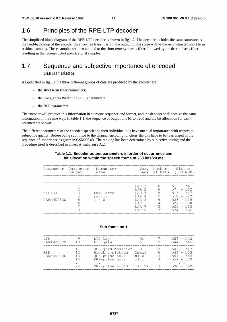
1.7 Sequence and subjective importance of encodedparameters

As indicated in fig 1.1 the three different groups of data are produced by the encoder are:

- the short term filter parameters;

- the Long Term Prediction (LTP) parameters;

- the RPE parameters.

The encoder will produce this information in a unique sequence and format, and the decoder shall receive the sameinformation in the same way. In table 1.1, the sequence of output bits b1 to b260 and the bit allocation for eachparameter is shown.

The different parameters of the encoded speech and their individual bits have unequal importance with respect tosubjective quality. Before being submitted to the channel encoding function the bits have to be rearranged in thesequence of importance as given in GSM 05.03. The ranking has been determined by subjective testing and theprocedure used is described in annex A, subclause A.2.

Table 1.1: Encoder output parameters in order of occurrence andbit allocation within the speech frame of 260 bits/20 ms

==================================================================Parameter Parameter Parameter Var. Number Bit no. number name name of bits (LSB-MSB)==================================================================

================================================================== 1 LAR 1 6 b1 - b6 2 LAR 2 6 b7 - b12FILTER 3 Log. Area LAR 3 5 b13 - b17 4 ratios LAR 4 5 b18 - b22PARAMETERS 5 1 - 8 LAR 5 4 b23 - b26 6 LAR 6 4 b27 - b30 7 LAR 7 3 b31 - b33 8 LAR 8 3 b34 - b36==================================================================

Sub-frame no.1

==================================================================LTP 9 LTP lag N1 7 b37 - b43PARAMETERS 10 LTP gain b1 2 b44 - b45------------------------------------------------------------------ 11 RPE grid position M1 2 b46 - b47RPE 12 Block amplitude Xmax1 6 b48 - b53PARAMETERS 13 RPE-pulse no.1 x1(0) 3 b54 - b56 14 RPE-pulse no.2 x1(1) 3 b57 - b59 .. ... ... 25 RPE-pulse no.13 x1(12) 3 b90 - b92==================================================================

ETSI


Sub-frame no.2

==================================================================LTP 26 LTP lag N2 7 b93 - b99PARAMETERS 27 LTP gain b2 2 b100- b101------------------------------------------------------------------ 28 RPE grid position M2 2 b102- b103RPE 29 Block amplitude Xmax2 6 b104- b109PARAMETERS 30 RPE-pulse no.1 x2(0) 3 b110- b112 31 RPE-pulse no.2 x2(1) 3 b113- b115 .. ... ... 42 RPE-pulse no.13 x2(12) 3 b146- b148==================================================================

Table 1.1: Encoder output parameters in order of occurrence andbit allocation within the speech frame of 260 bits/20 ms

Sub-frame no.3

==================================================================LTP 43 LTP lag N3 7 b149- b155PARAMETERS 44 LTP gain b3 2 b156- b157------------------------------------------------------------------ 45 RPE grid position M3 2 b158- b159RPE 46 Block amplitude Xmax3 6 b160- b165PARAMETERS 47 RPE-pulse no.1 x3(0) 3 b166- b168 48 RPE-pulse no.2 x3(1) 3 b169- b171 .. ... ... 59 RPE-pulse no.13 x3(12) 3 b202- b204==================================================================

Sub-frame no.4

==================================================================LTP 60 LTP lag N4 7 b205- b211PARAMETERS 61 LTP gain b4 2 b212- b213------------------------------------------------------------------ 62 RPE grid position M4 2 b214- b215RPE 63 Block amplitude Xmax4 6 b216- b221PARAMETERS 64 RPE-pulse no.1 x4(0) 3 b222- b224 65 RPE-pulse no.2 x4(1) 3 b225- b227 .. ... ... 76 RPE-pulse no.13 x4(12) 3 b258- b260==================================================================

ETSI


Input Pre-processingsignal

Short termanalysis

filter

Short termLPC

analysis

+RPE gridselection

and coding

(1) (2)

LTPanalysis

Long termanalysis

filter+

RPE griddecoding and

positioning

(4) (5)

(3)-

LTP parameters(9 bits/5 ms)

Reflectioncoefficients coded asLog. - Area Ratios(36 bits/20 ms)

RPE parameters(47 bits/5 ms)

To

radio

subsystem

(1) Short term residual(2) Long term residual (40 samples)(3) Short term residual estimate (40 samples)(4) Reconstructed short term residual (40 samples)(5) Quantized long term residual (40 samples)

Figure 1.1: Simplified block diagram of the RPE - LTPencoder

RPE griddecoding and

positioning

Reflection coefficients coded as Log. - Area Ratios(36 bits/20 ms)

RPE parameters(47 bits/5 ms)

From

radio

subsystem

LTP parameters(9 bits/5 ms)

+Short termsynthesis

filter

Long termsynthesis

filter

Post-processing

Output

signal

Figure 1.2: Simplified block diagram of the RPE - LTP decoder

ETSI


2 Transmission characteristicsThis clause specifies the necessary performance characteristics of the audio parts for proper functioning of the speechtranscoder. Some transmission performance characteristics of the RPE-LTP transcoder are also given to assist thedesigner of the speech transcoder function. The information given here is redundant and the detailed specifications arecontained in recommendation GSM 11.10.

The performance characteristics are referred to the 13 bit uniform PCM interface.

NOTE: To simplify the verification of the specifications, the performance limits may be referred to an A-lawmeasurement interface according to ITU-T Recommendation G.711. In this way, standard measuringequipments for PCM systems can be utilized for measurements. The relationship between the 13 bitformat and the A-law companded shall follow the procedures defined in subclause 1.4.

2.1 Performance characteristics of the analogue/digitalinterfaces

Concerning 1) discrimination against out-of-band signals (sending) and 2) spurious out-of-band signals (receiving), thesame requirements as defined in ETSI standard TE 04-15 (digital telephone, candidate NET33) apply.

2.2 Transcoder delayConsider a back to back configuration where the parameters generated by the encoder are delivered to the speechdecoder as soon as they are available.

The transcoder delay is defined as the time interval between the instant a speech frame of 160 samples has been receivedat the encoder input and the instant the corresponding 160 reconstructed speech samples have been out-put by thespeech decoder at an 8 kHz sample rate.

The theoretical minimum delay which can be achieved is 20 ms. The requirement is that the transcoder delay should beless than 30 ms.

3 Functional description of the RPE-LTP codecThe block diagram of the RPE-LTP-coder is shown in figure 3.1. The individual blocks are described in the followingsubclauses.

3.1 Functional description of the RPE-LTP encoderThe Pre-processing section of the RPE-LTP encoder comprises the following two sub-blocks:

- Offset compensation (3.1.1);

- Pre-emphasis (3.1.2).

The LPC analysis section of the RPE-LTP encoder comprises the following five sub-blocks:

- Segmentation (3.1.3);

- Auto-Correlation (3.1.4);

- Schur Recursion (3.1.5);

- Transformation of reflection coefficients to Log.-Area Ratios (3.1.6);

- Quantization and coding of Log.-Area Ratios (3.1.7).

The Short term analysis filtering section of the RPE-LTP comprises the following four sub-blocks:

ETSI


- Decoding of the quantized Log.-Area Ratios (LARs) (3.1.8);

- Interpolation of Log.-Area Ratios (3.1.9);

- Transformation of Log.-Area Ratios into reflection coefficients (3.1.10);

- Short term analysis filtering (3.1.11).

The Long Term Predictor (LTP) section comprises 4 sub-blocks working on subsegments (3.1.12) of the short termresidual samples:

- Calculation of LTP parameters (3.1.13);

- Coding of the LTP lags (3.1.14) and the LTP gains (3.1.15);

- Decoding of the LTP lags (3.1.14) and the LTP gains (3.1.15);

- Long term analysis filtering (3.1.16), and Long term synthesis filtering (3.1.17).

The RPE encoding section comprises five different sub-blocks:

- Weighting filter (3.1.18);

- Adaptive sample rate decimation by RPE grid selection (3.1.19);

- APCM quantization of the selected RPE sequence (3.1.20);

- APCM inverse quantization (3.1.21);

- RPE grid positioning (3.1.22).

Pre-processing section

3.1.1 Offset compensation

Prior to the speech encoder an offset compensation, by a notch filter is applied in order to remove the offset of the inputsignal so to produce the offset-free signal sof.

s of (k) = s o(k) - s o(k-1) + alpha*s of (k-1) (3.1.1)

alpha = 32735*2 -15

3.1.2 Pre-emphasis

The signal sof is applied to a first order FIR pre-emphasis filter leading to the input signal s of the analysis section. s(k) = s of (k) - beta*s of (k-1) (3.1.2)

beta= 28180*2 -15

LPC analysis section

3.1.3 Segmentation

The speech signal s(k) is divided into non-overlapping frames having a length of T0 = 20 ms (160 samples). A newLPC-analysis of order p=8 is performed for each frame.

3.1.4 Autocorrelation

The first p+1 = 9 values of the Auto-Correlation function are calculated by:

159

ACF(k)= ∑ s(i)s(i-k) ,k = 0,1...,8 (3.2)

ETSI


i=k

3.1.5 Schur Recursion

The reflection coefficients are calculated as shown in figure 3.2 using the Schur Recursion algorithm. The term"reflection coefficient" comes from the theory of linear prediction of speech (LPC), where a vocal tract representationconsisting of series of uniform cylindrical sections is assumed. Such a representation can be described by the reflectioncoefficients or the area ratios of connected sections.

3.1.6 Transformation of reflection coefficients to Log.-Area Ratios

The reflection coefficients r(i), (i=1..8), calculated by the Schur algorithm, are in the range:

-1 <= r(i) <= + 1

Due to the favourable quantization characteristics, the reflection coefficients are converted into Log.-Area Ratios whichare strictly defined as follows:

1 + r(i)

Logarea(i) = log 10 (----------) (3.3)

1 - r(i)

Since it is the companding characteristic of this transformation that is of importance, the following segmentedapproximation is used.

r(i) ; |r(i)| < 0.675

LAR(i) = sign[r(i)]*[2|r(i)|-0.675] ; 0.675 <= |r(i)| < 0.950

sign[r(i)]*[8|r(i)|-6.375] ; 0.950 <= |r(i)| <= 1.000

(3.4)

with the result that instead of having to divide and obtain the logarithm of particular values, it is merely necessary tomultiply, add and compare these values.

The following equation (3.5) gives the inverse transformation.

LAR'(i) ; |LAR'(i)|<0.675

r'(i)=sign[LAR'(i)]*[0.500*|LAR'(i)|

+0.337500] ; 0.675<=|LAR'(i)|<1.225

sign[LAR'(i)]*[0.125*|LAR'(i)|

+0.796875] ; 1.225<=|LAR'(i)|<=1.625

(3.5)

3.1.7 Quantization and coding of Log.-Area Ratios

The Log.-Area Ratios LAR(i) have different dynamic ranges and different asymmetric distribution densities. For thisreason, the transformed coefficients LAR(i) are limited and quantized differently according to the following equation(3.6), with LARc(i) denoting the quantized and integer coded version of LAR(i).

LAR c(i) = Nint{A(i)*LAR(i) + B(i)} (3.6)

with

Nint{z} = int{z+sign{z}*0.5} (3.6a)

Function Nint defines the rounding to the nearest integer value, with the coefficients A(i), B(i), and different extremevalues of LARc(i) for each coefficient LAR(i) given in table 3.1.

ETSI


Table 3.1: Quantization of the Log.-Area Ratios LAR(i)

LAR No i A(i) B(i) MinimumLARc(i)

MaximumLARc(i)

1 20.000 0.000 -32 +312 20.000 0.000 -32 +313 20.000 4.000 -16 +154 20.000 -5.000 -16 +155 13.637 0.184 - 8 + 76 15.000 -3.500 - 8 + 77 8.334 -0.666 - 4 + 38 8.824 -2.235 - 4 + 3

Short-term analysis filtering section

The current frame of the speech signal s is retained in memory until calculation of the LPC parameters LAR(i) iscompleted. The frame is then read out and fed to the short term analysis filter of order p=8. However, prior to theanalysis filtering operation, the filter coefficients are decoded and pre-processed by interpolation.

3.1.8 Decoding of the quantized Log.-Area Ratios

In this block the quantized and coded Log.-Area Ratios (LARc(i)) are decoded according to equation (3.7).

LAR''(i) = ( LAR c(i) - B(i) )/ A(i) (3.7)

3.1.9 Interpolation of Log.-Area Ratios

To avoid spurious transients which may occur if the filter coefficients are changed abruptly, two subsequent sets ofLog.-Area Ratios are interpolated linearly. Within each frame of 160 analysed speech samples the short term analysisfilter and the short term synthesis filter operate with four different sets of coefficients derived according to table 3.2.

Table 3.2: Interpolation of LAR parameters (J=actual segment)

k LAR' J(i) = 0...12 0.75*LAR' 'J-1(i) + 0.25*LAR' 'J(i) 13...26 0.50*LAR' 'J-1(i) + 0.50*LAR' 'J(i) 27...39 0.25*LAR' 'J-1(i) + 0.75*LAR' 'J(i) 40..159 LAR' 'J(i)

3.1.10 Transformation of Log.-Area Ratios into reflection coefficients

The reflection coefficients are finally determined using the inverse transformation according to equation (3.5).

3.1.11 Short term analysis filtering

The Short term analysis filter is implemented according to the lattice structure depicted in figure 3.3.

d 0(k) = s(k) (3.8a)

u 0(k) = s(k) (3.8b)

d i (k) = d i-1 (k) + r' i *u i-1 (k-1) with i=1,...8 (3.8c)

u i (k) = u i-1 (k-1) + r' i *d i-1 (k) with i=1,...8 (3.8d)

d(k ) = d 8(k) (3.8e)

Long-Term Predictor (LTP) section

ETSI


3.1.12 Sub-segmentation

Each input frame of the short term residual signal contains 160 samples, corresponding to 20 ms. The long termcorrelation is evaluated four times per frame, for each 5 ms subsegment. For convenience in the following, we notej=0,...,3 the sub-segment number, so that the samples pertaining to the j-th sub-segment of the residual signal are nowdenoted by d(kj+k) with j = 0,...,3; kj = k0 + j*40 and k = 0,...,39 where k0 corresponds to the first value of the currentframe.

3.1.13 Calculation of the LTP parameters

For each of the four sub-segments a long term correlation lag Nj, (j=0,...,3), and an associated gain factor bj, (j=0,...,3)are determined. For each sub-segment, the determination of these parameters is implemented in three steps.

1) The first step is the evaluation of the cross-correlation Rj(lambda) of the current sub-segment of short termresidual signal d(kj+i),(i=0,...,39) and the previous samples of the reconstructed short term residual signald'(kj+i), (i=-120,...,-1):

39 j = 0,...3

R j (lambda) = ∑ d(k j +i)*d'(k j +i-lambda); k j = k 0 + j*40

i=0 lambda = 40,...,120

(3.9)

The cross-correlation is evaluated for lags lambda greater than or equal to 40 and less than or equal to 120, i.e.corresponding to samples outside the current sub-segment and not delayed by more than two sub-segments.

2) The second step is to find the position Nj of the peak of the cross-correlation function within this interval:

R j (N j ) = max { R j (lambda); lambda = 40..120 };

j = 0,...,3

(3.10)

3) The third step is the evaluation of the gain factor bj according to:

b j = R j (N j ) / S j (N j ); j = 0,...,3 (3.11)

with

39

S j (N j ) = ∑ d' 2 (k j +i-N j ); j = 0,...,3 (3.12)

i=0

It is clear that the last 120 samples of the reconstructed short term residual signal d'(kj+i),(i=-120,...,-1) shall be retaineduntil the next sub-segment so as to allow the evaluation of the relations (3.9),...,(3.12).

3.1.14 Coding/Decoding of the LTP lags

The long term correlation lags Nj,(j=0,...,3) can have values in the range (40,...,120), and so shall be coded using 7 bitswith:

N cj = N j ; j = 0,...,3 (3.13)

At the receiving end, assuming an error free transmission, the decoding of these values will restore the actual lags:

N j ' = N cj ; j = 0,...,3 (3.14)

3.1.15 Coding/Decoding of the LTP gains

The long term prediction gains bj,(j=0,...,3) are encoded with 2 bits each, according to the following algorithm:

ETSI


if b j <= DLB(i) then b cj = 0; i=0

if DLB(i-1) < b j <= DLB(i) then b cj = i; i=1,2 (3.15)

if DLB(i-1) < b j then b cj = 3; i=3

where DLB(i),(i=0,...,2) denotes the decision levels of the quantizer, and bcj represents the coded gain value. Decisionlevels and quantizing levels are given in table 3.3.

Table 3.3: Quantization table for the LTP gain

i Decision level Quantizing levelDLB(i) QLB(i)

0 0.2 0.101 0.5 0.352 0.8 0.653 1.00

The decoding rule is implemented according to:

b j ' = QLB(b cj ) ; j = 0,...,3 (3.16)

where QLB(i),(i=0,...,3) denotes the quantizing levels, and bj' represents the decoded gain value (see table 3.3).

3.1.16 Long term analysis filtering

The short term residual signal d(k0+k),(k=0,...,159) is processed by sub-segments of 40 samples. From each of the foursub-segments (j=0,...,3) of short term residual samples, denoted here d(kj+k), (k=0,...,39), an estimate d"(kj+k),(k=0,...,39) of the signal is subtracted to give the long term residual signal e(kj+k), (k=0,...,39) (see figure 3.1):

j = 0,...,3

e(k j +k) = d(k j +k) - d"(k j +k) ; k = 0,...,39 (3.17)

k j = k 0 + j*40

Prior to this subtraction, the estimated samples d"(kj+k) are computed from the previously reconstructed short termresidual samples d', adjusted to the current sub-segment LTP lag Nj' and weighted with the sub-segment LTP gain bj':

j = 0,...,3

d"(k j +k) = b j '*d'(k j +k-N j ') ; k = 0,...,39 (3.18)

k j = k 0 + j*40

3.1.17 Long term synthesis filtering

The reconstructed long term residual signal e'(k0+k),(k=0,...,159) is processed by sub-segments of 40 samples. To eachsub-segment, denoted here e'(kj+k), (k=0,...,39), the estimate d"(kj+k), (k=0,...,39) of the signal is added to give thereconstructed short term residual signal d'(kj+k),(k=0,...,39):

j = 0,...,3

d'(k j +k) = e'(k j +k) + d"(k j +k) ; k = 0,...,39 (3.19)

k j = k 0 + j*40

RPE encoding section

3.1.18 Weighting Filter

A FIR "block filter" algorithm is applied to each sub-segment by convolving 40 samples e(k) with the impulse responseH(i) ; i=0,...,10 (see table 3.4).

ETSI


Table 3.4: Impulse response of block filter (weighting filter)

i 5 4 (6) 3 (7) 2 (8) 1 (9) 0 (10)H(i)*213 8192 5741 2054 0 -374 -134

|H(Omega=0)| = 2.779;

The conventional convolution of a sequence having 40 samples with an 11-tap impulse response would produce40+11-1=50 samples. In contrast to this, the "block filter" algorithm produces the 40 central samples of the conventionalconvolution operation. For notational convenience the block filtered version of each sub-segment is denoted by x(k),k=0,...,39.

10

x(k) = ∑ H(i) * e(k+5-i) with k = 0,...,39 (3.20)

i=0

NOTE: e(k+5-i) = 0 for k+5-i<0 and k+5-i>39.

3.1.19 Adaptive sample rate decimation by RPE grid selection

For the next step, the filtered signal x is down-sampled by a ratio of 3 resulting in 3 interleaved sequences of lengths 14,13 and 13, which are split up again into 4 sub-sequences xm of length 13:

x m(i) = x(k j +m+3*i) ; i = 0,...,12 (3.21)

m = 0,...,3

with m denoting the position of the decimation grid. According to the explicit solution of the RPE mean squared errorcriterion, the optimum candidate sub-sequence xM is selected which is the one with the maximum energy:

12

E M = max ∑ x m2(i) ; m = 0,...,3 (3.22)

m i=0

The optimum grid position M is coded as Mc with 2 bits.

3.1.20 APCM quantization of the selected RPE sequence

The selected sub-sequence xM(i) (RPE sequence) is quantized, applying APCM (Adaptive Pulse Code Modulation). Foreach RPE sequence consisting of a set of 13 samples xM(i) ,the maximum xmax of the absolute values |xM(i)| is selectedand quantized logarithmically with 6 bits as xmaxc as given in table 3.5.

ETSI


Table 3.5: Quantization of the block maximum x max

xmax x'max xmaxc xmax x'max xmaxc

0 .. 31 31 0 2048 .. 2303 2303 32 32 .. 63 63 1 2304 .. 2559 2559 33 64 .. 95 95 2 2560 .. 2815 2815 34 96 .. 127 127 3 2816 .. 3071 3071 35 128 .. 159 159 4 3072 .. 3327 3327 36 160 .. 191 191 5 3328 .. 3583 3583 37 192 .. 223 223 6 3584 .. 3839 3839 38 224 .. 255 255 7 3840 .. 4095 4095 39 256 .. 287 287 8 4096 .. 4607 4607 40 288 .. 319 319 9 4608 .. 5119 5119 41 320 .. 351 351 10 5120 .. 5631 5631 42 352 .. 383 383 11 5632 .. 6143 6143 43 384 .. 415 415 12 6144 .. 6655 6655 44 416 .. 447 447 13 6656 .. 7167 7167 45 448 .. 479 479 14 7168 .. 7679 7679 46 480 .. 511 511 15 7680 .. 8191 8191 47 512 .. 575 575 16 8192 .. 9215 9215 48 576 .. 639 639 17 9216 .. 10239 10239 49 640 .. 703 703 18 10240 .. 11263 11263 50 704 .. 767 767 19 11264 .. 12287 12287 51 768 .. 831 831 20 12288 .. 13311 13311 52 832 .. 895 895 21 13312 .. 14335 14335 53 896 .. 959 959 22 14336 .. 15359 15359 54 960 .. 1023 1023 23 15360 .. 16383 16383 55 1024 .. 1151 1151 24 16384 .. 18431 18431 56 1152 .. 1279 1279 25 18432 .. 20479 20479 57 1280 .. 1407 1407 26 20480 .. 22527 22527 58 1408 .. 1535 1535 27 22528 .. 24575 24575 59 1536 .. 1663 1663 28 24576 .. 26623 26623 60 1664 .. 1791 1791 29 26624 .. 28671 28671 61 1792 .. 1919 1919 30 28672 .. 30719 30719 62 1920 .. 2047 2047 31 30720 .. 32767 32767 63

For the normalization, the 13 samples are divided by the decoded version x'max of the block maximum. Finally, thenormalized samples:

x'(i) = x M(i)/x' max ; i=0,...,12 (3.23)

are quantized uniformly with three bits to xMc(i) as given in table 3.6.

Table 3.6: Quantization of the normalized RPE-samples

x'*215 xM'*215 xMc

(Interval-limits) (Channel) -32768 ... -24577 -28672 0 = 000 -24576 ... -16385 -20480 1 = 001 -16384 ... -8193 -12288 2 = 010 -8192 ... -1 -4096 3 = 011

0 ... 8191 4096 4 = 100 8192 ... 16383 12288 5 = 101 16384 ... 24575 20480 6 = 110 24576 ... 32767 28672 7 = 111

3.1.21 APCM inverse quantization

The xMc(i) are decoded to xM'(i) and denormalized using the decoded value x'maxc leading to the decoded sub-sequencex'M(i).

ETSI


3.1.22 RPE grid positioning

The quantized sub-sequence is upsampled by a ratio of 3 by inserting zero values according to the grid position givenwith Mc.

3.2 DecoderThe decoder comprises the following 4 sections. Most of the sub-blocks are also needed in the encoder and have beendescribed already. Only the short term synthesis filter and the de-emphasis filter are added in the decoder as newsub-blocks.

- RPE decoding section (3.2.1);

- Long Term Prediction section (3.2.2);

- Short term synthesis filtering section (3.2.3);

- Post-processing (3.2.4).

The complete block diagram for the decoder is shown in figure 3.4. The variables and parameters of the decoder aremarked by the index r to distinguish the received values from the encoder values.

3.2.1 RPE decoding section

The input signal of the long term synthesis filter (reconstruction of the long term residual signal) is formed by decodingand denormalizing the RPE-samples (APCM inverse quantization - 3.1.21) and by placing them in the correct timeposition (RPE grid positioning - 3.1.22). At this stage, the sampling frequency is increased by a factor of 3 by insertingthe appropriate number of intermediate zero-valued samples.

3.2.2 Long Term Prediction section

The reconstructed long term residual signal er' is applied to the long term synthesis filter (see 3.1.16 and 3.1.17) whichproduces the reconstructed short term residual signal dr' for the short term synthesizer.

3.2.3 Short term synthesis filtering section

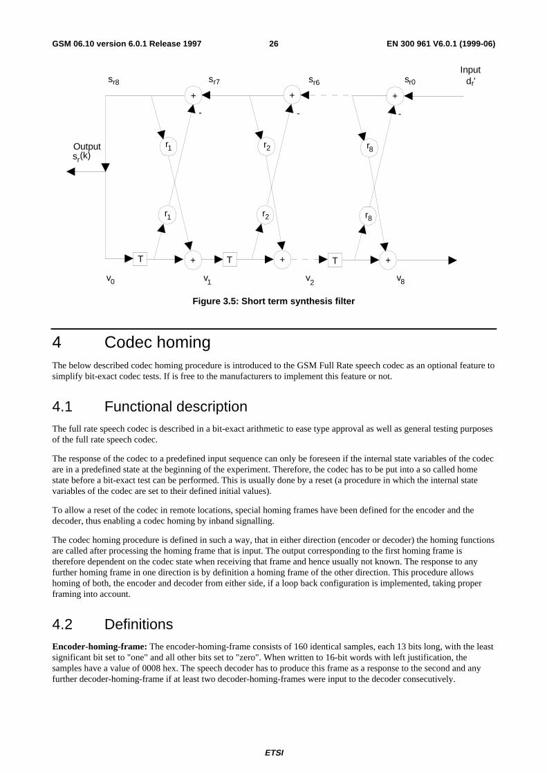
The coefficients of the short term synthesis filter (see figure 3.5) are reconstructed applying the identical procedure tothat in the encoder (3.1.8 - 3.1.10). The short term synthesis filter is implemented according to the lattice structuredepicted in figure 3.5.

s r(0) (k) = d r '(k) (3.24a)

s r(i) (k) = s r(i-1) (k) - r r ' (9-i) * v 8-i (k-1); i=1,...,8

(3.24b)

v 9-i (k) = v 8-i (k-1) + r r ' (9-i) * s r(i) (k); i=1,...,8

(3.24c)

s r '(k) = s r(8) (k) (3.24d)

v 0(k) = s r(8) (k) (3.24e)

3.2.4 Post-processing

The output of the synthesis filter sr(k) is fed into the IIR- de-emphasis filter leading to the output signal sro.

s ro (k) = s r (k) + beta*s ro (k-1) ; beta= 28180*2 -15 (3.25)

ETSI


Offs

etco

mpe

nsat

ion

Pre

emph

asis

Aut

o-co

rrel

atio

n

Seg

men

tatio

n

Log

Are

aR

atio

s

Sch

urre

curs

ion

Qua

ntiz

er/

code

r

s 0

s 0f

s

Pre

proc

essi

ng

AC

F

r LAR

Ref

lect

ion

coef

ficie

nts

Inve

rse

filte

r A

(z)

LAR

deco

der

Inte

r-po

latio

n

s

LAR

"

LAR

'

r'

LAR

c

LPC

ana

lysi

sS

hort

term

anal

ysis

filte

ring

LTP

para

met

er

LTP

par

amet

erde

code

r

Qua

ntiz

er/

code

rN

c

Xz

-N

d

d'

bN

b c

N'

b'

++

d'

d"

Wei

ghtin

gfil

ter

H(z

)e

Long

term

Pre

dict

ion

d"-

RP

E g

ridse

lect

ion

AP

CM

quan

tizer

Mc

x m

Inve

rse

AP

CM

x m c

x max

c

RP

E g

ridpo

sitio

n

x m'

e'

sign

als

para

met

ers

to th

e ra

dio

subs

yste

m

RP

E e

ncod

ing

Figure 3.1: Block diagram of the RPE - LTP encoder

ETSI


n = 1

ACF = 0 ?

K(9 - i) = ACF(i); i=7, ..., 7P(j) = ACF(j); j=0, ..., 8

P(0) < | P(1) |

r(n) = | P(1) | / P(0)

P(1) > 0 ?

n = 8 ?

P(0) = P(0) + P(1) * r(n)

m = 1

r(i) = 0; i = n, ..., 8

r(n) = - r(n)

Transformationr - > LAR

yes

yes

yes

yes

no

no

no

no

P(m) = P(1 + m) + r(n) * K(9 - m)K(9- m) = K(9 - m) + r(n) * P(1 + m)

END

m = 8 - n ? m = m + 1n = n + 1yes no

Figure 3.2: LPC analysis using Schur recursion

ETSI


T +

+

T

r1

r1

+

r2

r2

+ T +

+

r8

r8

u0 u1 u2 u8

Inputs(k)

d0 d1 d2 d8

Output

u8

d(k)

Figure 3.3: Short term analysis filter

RPE gridposition

InverseAPCM

er'

xmr'

signals

parameters from the radio subsystem

Mcr

xmaxcr

xmcr

bcr LTPparameterdecoder

Ncr

LARcr LARdecoder

Interpolation

Reflectioncoefficients

Short termsynthesis

filter 1/A(z)

LARr"

LARr'

rr'

+

X

br'

z- N

Nr'

dr"

dr'

Deemphasis

sr sr0

RPEdecoding

Long termPrediction

Short termsynthesisfiltering

Postprocessing

Figure 3.4: Block diagram of the RPE-LTP decoder

ETSI


T +

+

T

r1

r1

+

r2

r2

+ T +

+

r8

r8

v0 v1 v2 v8

Outputsr(k)

r8

Inputdr'

- - -

r7 r6 r0ssss

Figure 3.5: Short term synthesis filter

4 Codec homingThe below described codec homing procedure is introduced to the GSM Full Rate speech codec as an optional feature tosimplify bit-exact codec tests. If is free to the manufacturers to implement this feature or not.

4.1 Functional descriptionThe full rate speech codec is described in a bit-exact arithmetic to ease type approval as well as general testing purposesof the full rate speech codec.

The response of the codec to a predefined input sequence can only be foreseen if the internal state variables of the codecare in a predefined state at the beginning of the experiment. Therefore, the codec has to be put into a so called homestate before a bit-exact test can be performed. This is usually done by a reset (a procedure in which the internal statevariables of the codec are set to their defined initial values).

To allow a reset of the codec in remote locations, special homing frames have been defined for the encoder and thedecoder, thus enabling a codec homing by inband signalling.

The codec homing procedure is defined in such a way, that in either direction (encoder or decoder) the homing functionsare called after processing the homing frame that is input. The output corresponding to the first homing frame istherefore dependent on the codec state when receiving that frame and hence usually not known. The response to anyfurther homing frame in one direction is by definition a homing frame of the other direction. This procedure allowshoming of both, the encoder and decoder from either side, if a loop back configuration is implemented, taking properframing into account.

4.2 DefinitionsEncoder-homing-frame: The encoder-homing-frame consists of 160 identical samples, each 13 bits long, with the leastsignificant bit set to "one" and all other bits set to "zero". When written to 16-bit words with left justification, thesamples have a value of 0008 hex. The speech decoder has to produce this frame as a response to the second and anyfurther decoder-homing-frame if at least two decoder-homing-frames were input to the decoder consecutively.

ETSI


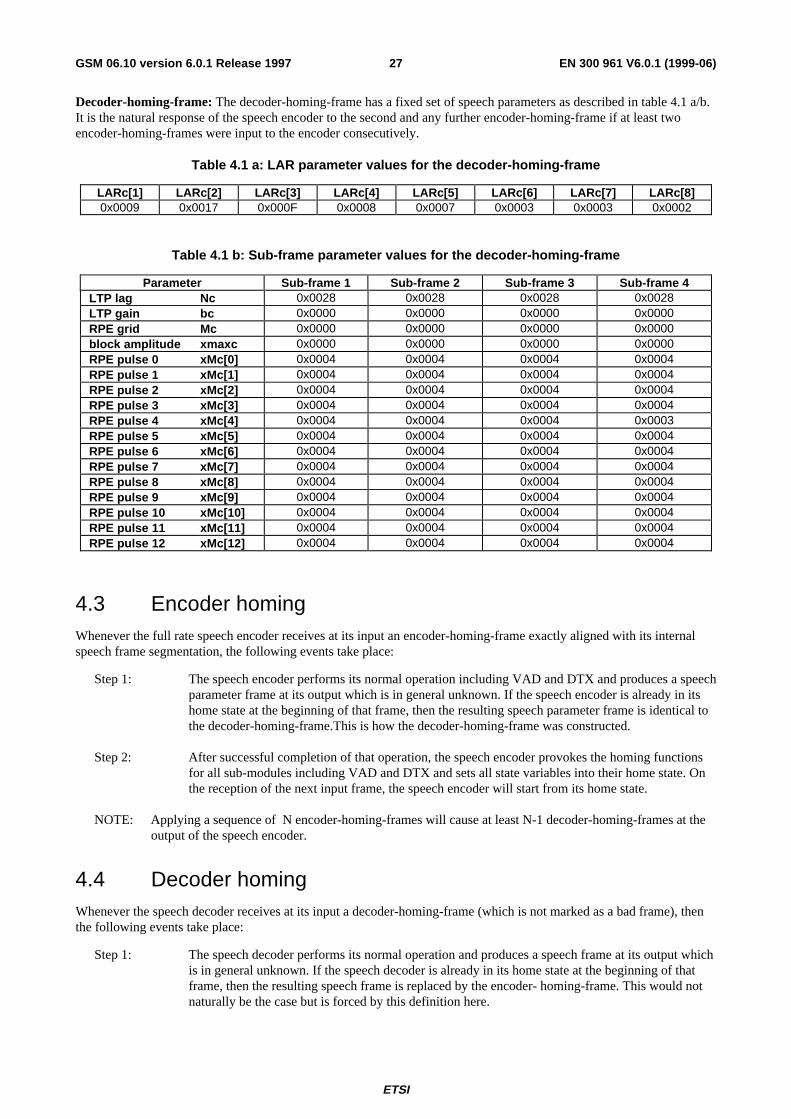
Decoder-homing-frame: The decoder-homing-frame has a fixed set of speech parameters as described in table 4.1 a/b.It is the natural response of the speech encoder to the second and any further encoder-homing-frame if at least twoencoder-homing-frames were input to the encoder consecutively.

Table 4.1 a: LAR parameter values for the decoder-homing-frame

LARc[1] LARc[2] LARc[3] LARc[4] LARc[5] LARc[6] LARc[7] LARc[8]0x0009 0x0017 0x000F 0x0008 0x0007 0x0003 0x0003 0x0002

Table 4.1 b: Sub-frame parameter values for the decoder-homing-frame

Parameter Sub-frame 1 Sub-frame 2 Sub-frame 3 Sub-frame 4 LTP lag Nc 0x0028 0x0028 0x0028 0x0028 LTP gain bc 0x0000 0x0000 0x0000 0x0000 RPE grid Mc 0x0000 0x0000 0x0000 0x0000 block amplitude xmaxc 0x0000 0x0000 0x0000 0x0000 RPE pulse 0 xMc[0] 0x0004 0x0004 0x0004 0x0004 RPE pulse 1 xMc[1] 0x0004 0x0004 0x0004 0x0004 RPE pulse 2 xMc[2] 0x0004 0x0004 0x0004 0x0004 RPE pulse 3 xMc[3] 0x0004 0x0004 0x0004 0x0004 RPE pulse 4 xMc[4] 0x0004 0x0004 0x0004 0x0003 RPE pulse 5 xMc[5] 0x0004 0x0004 0x0004 0x0004 RPE pulse 6 xMc[6] 0x0004 0x0004 0x0004 0x0004 RPE pulse 7 xMc[7] 0x0004 0x0004 0x0004 0x0004 RPE pulse 8 xMc[8] 0x0004 0x0004 0x0004 0x0004 RPE pulse 9 xMc[9] 0x0004 0x0004 0x0004 0x0004 RPE pulse 10 xMc[10] 0x0004 0x0004 0x0004 0x0004 RPE pulse 11 xMc[11] 0x0004 0x0004 0x0004 0x0004 RPE pulse 12 xMc[12] 0x0004 0x0004 0x0004 0x0004

4.3 Encoder homingWhenever the full rate speech encoder receives at its input an encoder-homing-frame exactly aligned with its internalspeech frame segmentation, the following events take place:

Step 1: The speech encoder performs its normal operation including VAD and DTX and produces a speechparameter frame at its output which is in general unknown. If the speech encoder is already in itshome state at the beginning of that frame, then the resulting speech parameter frame is identical tothe decoder-homing-frame.This is how the decoder-homing-frame was constructed.

Step 2: After successful completion of that operation, the speech encoder provokes the homing functionsfor all sub-modules including VAD and DTX and sets all state variables into their home state. Onthe reception of the next input frame, the speech encoder will start from its home state.

NOTE: Applying a sequence of N encoder-homing-frames will cause at least N-1 decoder-homing-frames at theoutput of the speech encoder.

4.4 Decoder homingWhenever the speech decoder receives at its input a decoder-homing-frame (which is not marked as a bad frame), thenthe following events take place:

Step 1: The speech decoder performs its normal operation and produces a speech frame at its output whichis in general unknown. If the speech decoder is already in its home state at the beginning of thatframe, then the resulting speech frame is replaced by the encoder- homing-frame. This would notnaturally be the case but is forced by this definition here.

ETSI


Step 2: After successful completion of that operation, the speech decoder provokes the homing functionsfor all sub-modules including the comfort noise generator and sets all state variables into theirhome state. On the reception of the next input frame, the speech decoder will start from its homestate.

NOTE 1: Applying a sequence of N decoder-homing-frames will cause at least N-1 encoder-homing-frames at theoutput of the speech decoder.

NOTE 2: By definition, the first frame of each decoder test sequence must differ from the decoder-homing-frame atleast in one bit position within the parameters for LARs and first subframe. Therefore, if the decoder is inits home state, it is sufficient to check only these parameters to detect a subsequent decoder-homing-frame. This definition is made to support a delay-optimized implementation in the TRAU uplink direction.

4.5 Encoder home stateIn table 4.2, a listing of all the encoder state variables with their predefined values when in the home state is given.

Table 4.2: Initial values of the encoder state variables

Variable Initial valueOffset compensation filter memory z1 set to 0Offset compensation filter memory L_z2 set to 0

Pre-emphasis filter memory mp set to 0LARs from previous frame LARpp(j-1)[1...8] all set to 0

Short term analysis filter memory u[0...7] all set to 0LTP delay line dp[-120...-1] all set to 0

Initial values for variables used by the VAD algorithm are listed in GSM 06.32 [12]. In addition, the state variables ofthe DTX system have to be brought into their home state. As the DTX system is not specified in a bit-exact way, nocommon reset table can be given here.

4.6 Decoder home stateIn table 4.3, a listing of all the decoder state variables with their predefined values when in the home state is given.

Table 4.3: Initial values of the decoder state variables

Variable Initial valueLTP lag from previous frame nrp set to 40

LTP delay line drp[-120...-1] all set to 0LARs from previous frame LARrpp(j-1)[1...8] all set to 0

Short term synthesis filter memory v[0...8] all set to 0De-emphasis filter memory msr set to 0

In addition, the state variables of the bad frame handling (error concealment) module and the comfort noise insertionmodule have to be brought into their home state. As these modules are not specified in a bit-exact way, no common resettable can be given here.

5 Computational details of the RPE-LTP codec

5.1 Data representation and arithmetic operationsOnly two types of variables are used along the implementation of the RPE-LTP algorithm in fixed point arithmetic.These two types are:

Integer on 16 bits;

ETSI


Long integer on 32 bits.

This assumption simplifies the detailed description and allows the maximum reach of precision.

In different places of the recommendation, different scaling factors are used according to different operations. To helpthe reader in the comparison of corresponding floating point and fixed point values given in section 3 and 4 commentsof the format:

/* var = integer( real_var * scalefactor ) */

are used at several points of section 5. var is the rounded fixed point representation of the floating point representationof var (real_var) using the given scaling factor.

In the description, input signal samples, coded parameters and output signal samples are represented by 16 bit words. Atthe receiving part it shall therefore be ensured that only valid bits (13 bits for samples signal and two to seven bits forcoded parameters) are used. In verification tests, the testing system may introduce random bit at non valid places insidethese samples (3 LSBs) or parameters (MSBs) to test this function. In the digital test sequences all non valid bits are setto 0.

The following part of this section describes the required set of arithmetic operations to implement the RPE-LTPalgorithm in fixed point.

For arithmetics operations or variables with a long integer type (32 bit) a prefix L_ is used in order to distinguish themfrom the 16 bit variables or arithmetic operations.

All the names of the variables are identical to those of the functional description of the RPE-LTP Codec (section 3) butvariables like x', x'' are respectively called:

x' -----> xp x''-----> xpp

in order to avoid any confusing notation.

NOTE: The x', x" variables are examples but are not used within the following description.

The following notations are used in the arithmetic operations:

Square brackets ( [..] ) are used for arrays and when needed, the starting index and the ending index are put inside thebracket. For example x[0..159] means that x is an array of 160 words of 16 bits with beginning index 0 and ending index159 and x[k] is an element of the array x[0..159].

All functions' names are underlined. For example add( x, y) means that we perform the addition of x and y.

<< n: denotes a n-bit arithmetic shift left operation (zero fill) on variables of type short or long; if n isless than 0, this operation becomes an arithmetic right shift of -n;

>> n: denotes a n-bit arithmetic right shift operation (sign extension ) on variables of type short or long;if n is less than 0, this operation becomes an arithmetic left shift of -n (zero fill);

a > b: denotes the "greater than" condition;

a >= b: denotes the "greater than or equal" condition;

a < b: denotes the "less than" condition;

a <= b: denotes the "less than or equal" condition;

a == b: denotes the "equal to" condition.

The basic structure of the FOR-NEXT loop is used in this description for loop computation; the declaration is:

|== FOR k= start to end: | inner computation; |== NEXT k:

Also the IF.. ELSE IF structure is used throughout this detailed description. The basic structure is:

IF (condition1) THEN statement1;

ETSI


ELSE IF ( condition2) THEN statement2; ELSE IF ( condition3) THEN statement3;

The word EXIT is used to exit immediately from a procedure.

The following arithmetic operations are defined:

add( var1, var2): performs the addition (var1+var2) with overflow control and saturation; the result is set at +32767when overflow occurs or at -32768 when underflow occurs.

sub( var1, var2): performs the subtraction (var1-var2) with overflow control and saturation; the result is set at+32767 when overflow occurs or at -32768 when underflow occurs.

mult( var1, var2): performs the multiplication of var1 by var2 and gives a 16 bits result which is scaled i.e.mult(var1,var2 ) = (var1 times var2) >> 15 and mult(-32768, -32768) = 32767

mult_r( var1, var2): same as mult but with rounding i.e. mult_r( var1, var2 ) = ( (var1 times var2) + 16384 ) >> 15and mult_r( -32768, -32768 ) = 32767

abs( var1 ): absolute value of var1; abs(-32768) = 32767

div( var1, var2): div produces a result which is the fractional integer division of var1 by var2; var1 and var2 shallbe positive and var2 shall be greater or equal to var1; The result is positive (leading bit equal to 0)and truncated to 16 bits. if var1 == var2 then div( var1, var2 ) = 32767

L_mult(var1, var2): L_mult is a 32 bit result for the multiplication of var1 times var2 with a one bit shift left.L_mult( var1, var2 ) = ( var1 times var2 ) << 1. The condition L_mult (-32768, -32768 ) does notoccur in the algorithm.

L_add(L_var1, L_var2): 32 bits addition of two 32 bits variables (L_var1 + L_var2) with overflow control andsaturation; the result is set at 2147483647 when overflow occurs and at -2147483648 whenunderflow occurs.

L_sub(L_var1,L_var2): 32 bits subtraction of two 32 bits variables (L_var1 - L_var2) with overflow control andsaturation; the result is set at 2147483647 when overflow occurs and at -2147483648 whenunderflow occurs.

norm( L_var1 ): norm produces the number of left shifts needed to normalize the 32 bits variable L_var1 forpositive values on the interval with minimum of 1073741824 and maximum of 2147483647 andfor negative values on the interval with minimum of -2147483648 and maximum of -1073741824;in order to normalize the result, the following operation shall be done: L_norm_var1 = L_var1 <<norm(L_var1)

L_var2 = var1: deposit the 16 bits of var1 in the LSB 16 bits of L_var2 with sign extension.

var2 = L_var1: extract the 16 LSB bits of L_var1 to put in var2.

When a constant is used in an operation on 32 bits, it shall be first sign-extended on 32 bits.

5.2 Fixed point implementation of the RPE-LTP coderThe RPE-LTP coder works on a frame by frame basis. The length of the frame is equal to 160 samples. Somecomputations are done once per frame (analysis) and some others for each of the four sub-segments (40 samples).

In the following detailed description, procedure 5.2.0 to 5.2.10 are done once per frame to produce at the output of thecoder the LARc[1..8] parameters which are the coded LAR coefficients and also to realize the inverse filtering operationfor the entire frame (160 samples of signal d[0..159]). These parts produce at the output of the coder:

| LARc[1..8] : Coded LAR coefficients

|--> These parameters are calculated and sent once per frame.

Procedure 5.2.11 to 5.2.18 are to be executed four times per frame. That means once for each sub-segment RPE-LTPanalysis of 40 samples. These parts produce at the output of the coder:

ETSI


| Nc : LTP lag;

| bc : Coded LTP gain;

| Mc : RPE grid selection;

| xmaxc : Coded maximum amplitude of the RPE sequence;

| xMc[0..12] : Codes of the normalized RPE samples;

|--> These parameters are calculated and sent four times per frame.

Pre-processing section

5.2.0 Scaling of the input variable

After A-law to linear conversion (or directly from the A to D converter) the following scaling is assumed for input to theRPE-LTP algorithm:

S.v.v.v.v.v.v.v.v.v.v.v.v.x.x.x ( 2's complement format).

Where S is the sign bit, v a valid bit, and x a "don't care" bit.

The original signal is called sop[..];

5.2.1 Downscaling of the input signal |== FOR k=0 to 159: | so[k] = sop[k] >> 3; | so[k] = so[k] << 2; |== NEXT k:

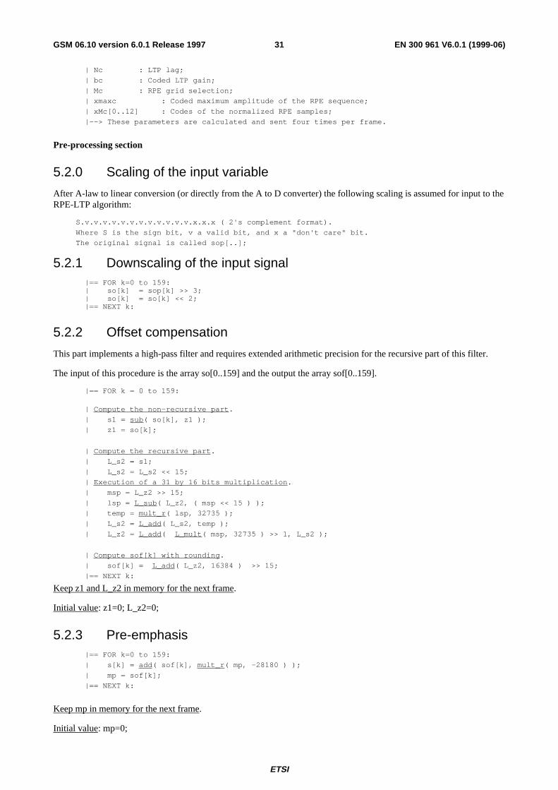
5.2.2 Offset compensation

This part implements a high-pass filter and requires extended arithmetic precision for the recursive part of this filter.

The input of this procedure is the array so[0..159] and the output the array sof[0..159].

|== FOR k = 0 to 159:

| Compute the non-recursive part .

| s1 = sub ( so[k], z1 );

| z1 = so[k];

| Compute the recursive part .

| L_s2 = s1;

| L_s2 = L_s2 << 15;

| Execution of a 31 by 16 bits multiplication .

| msp = L_z2 >> 15;

| lsp = L_sub ( L_z2, ( msp << 15 ) );

| temp = mult_r ( lsp, 32735 );

| L_s2 = L_add ( L_s2, temp );

| L_z2 = L_add ( L_mult ( msp, 32735 ) >> 1, L_s2 );

| Compute sof[k] with rounding .

| sof[k] = L_add ( L_z2, 16384 ) >> 15;

|== NEXT k:

Keep z1 and L_z2 in memory for the next frame.

Initial value: z1=0; L_z2=0;

5.2.3 Pre-emphasis |== FOR k=0 to 159:

| s[k] = add ( sof[k], mult_r ( mp, -28180 ) );

| mp = sof[k];

|== NEXT k:

Keep mp in memory for the next frame.

Initial value: mp=0;

ETSI


LPC analysis section

5.2.4 Autocorrelation

The goal is to compute the array L_ACF[k]. The signal s[i] shall be scaled in order to avoid an overflow situation.

Dynamic scaling of the array s[0..159].

Search for the maximum.

smax = 0;

|== FOR k = 0 to 159:

| temp = abs ( s [k] );

| IF ( temp > smax ) THEN smax = temp;

|== NEXT k;

Computation of the scaling factor.

IF ( smax == 0 ) THEN scalauto = 0;

ELSE scalauto = sub ( 4, norm ( smax << 16 ) );

Scaling of the array s[0..159].

IF ( scalauto > 0 ) THEN

| temp = 16384 >> sub ( scalauto,1);

|== FOR k = 0 to 159:

| s[k] = mult_r ( s[k], temp);

|== NEXT k:

Compute the L_ACF[..].

|== FOR k=0 to 8:

| L_ACF[k] = 0;

|==== FOR i=k to 159:

| L_temp = L_mult ( s[i], s[i-k] );

| L_ACF[k] = L_add ( L_ACF[k], L_temp );

|==== NEXT i:

|== NEXT k:

Rescaling of the array s[0..159].

IF ( scalauto > 0 ) THEN

|== FOR k = 0 to 159:

| s[k] = s[k] << scalauto;

|== NEXT k:

5.2.5 Computation of the reflection coefficients

Schur recursion with 16 bits arithmetic.

IF( L_ACF[0] == 0 ) THEN

|== FOR i = 1 to 8:

| r[i] = 0;

|== NEXT i:

| EXIT; /continue with section 5.2.6/

temp = norm ( L_ACF[0] );

|== FOR k=0 to 8:

| ACF[k] = ( L_ACF[k] << temp ) >> 16;

|== NEXT k:

Initialize array P[..] and K[..] for the recursion.

|== FOR i=1 to 7:

| K[9-i] = ACF[i];

|== NEXT i:

|== FOR i=0 to 8:

ETSI


| P[i] = ACF[i];

|== NEXT i:

Compute reflection coefficients.

|== FOR n=1 to 8:

| IF( P[0] < abs ( P[1] ) ) THEN

| |== FOR i = n to 8:

| | r[i] = 0;

| |== NEXT i:

| | EXIT; /continue with

| | section 5.2.6/

| r[n] = div ( abs ( P[1] ), P[0] );

| IF ( P[1] > 0 ) THEN r[n] = sub ( 0, r[n] );

|

| IF ( n == 8 ) THEN EXIT; /continue with

section 5.2-6/

Schur recursion.

| P[0] = add ( P[0], mult_r ( P[1], r[n] ) );

|==== FOR m=1 to 8-n:

| P[m] = add ( P[m+1], mult_r ( K[9-m], r[n] ) );

| K[9-m] = add ( K[9-m], mult_r ( P[m+1], r[n] ) );

|==== NEXT m:

|

|== NEXT n:

NOTE: The following lines gives one correct implementation of the div(num, denum) arithmetic operation.Compute div which is the integer division of num by denum: with denum >= num > 0.

L_num = num;

L_denum = denum;

div =0;

|== FOR k = 0 to 14:

| div= div << 1;

| L_num = L_num << 1;

| IF ( L_num >= L_denum) THEN

| | L_num=L_sub (L_num, L_denum);

| | div = add ( div ,1 );

|== NEXT k:

5.2.6 Transformation of reflection coefficients to Log.-Area Ratios

The following scaling for r[..] and LAR[..] has been used:

/* r[..] = integer( real_r[..]*32768. ); -1. <= real_r <1. */

/* */

/* LAR[..] = integer( real_LAR[..]*16384. ); */

/* */

/* with -1.625 <= real_LAR <= 1.625 */

Computation of the LAR[1..8] from the r[1..8].

|== FOR i = 1 to 8:

| temp = abs ( r[i] );

| IF ( temp < 22118 ) THEN temp = temp >> 1;

| ELSE IF ( temp < 31130 ) THEN

| temp= sub (temp, 11059);

| ELSE temp = sub ( temp, 26112 ) << 2;

| LAR[i] = temp;

| IF ( r[i] < 0 ) THEN LAR[i] = sub ( 0, LAR[i] );

|== NEXT i:

ETSI


5.2.7 Quantization and coding of the Log.-Area Ratios

This procedure needs four tables; the following equations give the optimum scaling for the constants:

/* A[1..8]= integer( real_A[1..8]*1024); 8 values (see table5.1)*/

/* */

/* B[1..8]= integer( real_B[1..8]*512); 8 values (see table5.1)*/

/* */

/* MAC[1..8]= maximum of the LARc[1..8]; 8 values (see table5.1)*/

/* */

/* MIC[1..8]= minimum of the LARc[1..8]; 8 values (see table5.1)*/

Computation for quantizing and coding the LAR[1..8].

|== FOR i =1 to 8:

| temp= mult ( A[i], LAR[i] );

| temp= add ( temp, B[i] );

| temp= add ( temp, 256); for rounding

| LARc[i]= temp >> 9;

|

| Check IF LARc[i] lies between MIN and MAX

|

| IF ( LARc[i] > MAC[i] ) THEN LARc[i] = MAC[i];

| IF ( LARc[i] < MIC[i] ) THEN LARc[i] = MIC[i];

| LARc[i] = sub ( LARc[i], MIC[i] ); /See note below/

|== NEXT i:

NOTE: The equation is used to make all the LARc[i] positive.

Short term analysis filtering section

5.2.8 Decoding of the coded Log.-Area Ratios

This procedure requires for efficient implementation two tables.

/* INVA[1..8]=integer((32768*8)/(real_A[1..8]); */

/* 8 values (table 5.2 ) */

/* MIC[1..8]=minimum value of the LARc[1..8]; */

/* 8 values (table 5.1) */

Compute the LARpp[1..8].

|== FOR i=1 to 8:

| temp1 = add ( LARc[i], MIC[i] ) << 10; /See note below/

| temp2 = B[i] << 1;

| temp1 = sub ( temp1, temp2);

| temp1 = mult_r ( INVA[i], temp1);

| LARpp[i] = add ( temp1, temp1);

|== NEXT i:

NOTE: The addition of MIC[i] is used to restore the sign of LARc[i].

5.2.9 Computation of the quantized reflection coefficients

Within each frame of 160 analysed speech samples the short term analysis and synthesis filters operate with fourdifferent sets of coefficients, derived from the previous set of decoded LARs(LARpp(j-1)) and the actual set of decodedLARs (LARpp(j)).

5.2.9.1 Interpolation of the LARpp[1..8] to get the LARp[1..8]

For k_start = 0 to k_end = 12.

|==== FOR i= 1 to 8:

| LARp[i] = add ((LARpp(j-1)[i] >> 2),(LARpp(j)[i] >> 2));

| LARp[i] = add ( LARp[i] , ( LARpp(j-1)[i] >> 1 ) );

ETSI


|==== NEXT i:


|==== FOR i= 1 to 8:

| LARp[i] = add ((LARpp(j-1)[i] >> 1),(LARpp(j)[i] >> 1 ));

|==== NEXT i:


|==== FOR i= 1 to 8:

| LARp[i] = add ((LARpp(j-1)[i] >> 2),(LARpp(j)[i] >> 2 ));

| LARp[i] = add ( LARp[i] , ( LARpp(j)[i] >> 1 ) );

|==== NEXT i:


|==== FOR i= 1 to 8:

| LARp[i] = LARpp(j)[i];

|==== NEXT i:

Initial value: LARpp(j-1)[1..8]=0;

5.2.9.2 Computation of the rp[1..8] from the interpolated LARp[1..8]

The input of this procedure is the interpolated LARp[1..8] array. The reflection coefficients, rp[i], are used in theanalysis filter and in the synthesis filter.

|== FOR i=1 to 8:

| temp = abs ( LARp[i] );

| IF ( temp < 11059 ) THEN temp = temp << 1;

| ELSE IF (temp < 20070) THEN

| temp = add (temp, 11059);

| ELSE temp = add ( (temp >> 2), 26112 );

| rp[i] = temp;

| IF ( LARp[i] < 0 ) THEN rp[i] = sub ( 0, rp[i] );

|== NEXT i:

5.2.10 Short term analysis filtering

This procedure computes the short term residual signal d[..] to be fed to the RPE-LTP loop from the s[..] signal andfrom the local rp[..] array (quantized reflection coefficients). As the call of this procedure can be done in many ways(see the interpolation of the LAR coefficient), it is assumed that the computation begins with index k_start (for arraysd[..] and s[..]) and stops with index k_end (k_start and k_end are defined in 5.2.9.1). This procedure also needs to keepthe array u[0..7] in memory for each call.

|== FOR k = k_start to k_end:

| di = s[k]

| sav = di;

|==== FOR i = 1 to 8:

| temp = add ( u[i-1], mult_r ( rp[i], di ) );

| di = add ( di, mult_r ( rp[i], u[i-1] ) );

| u[i-1] = sav;

| sav = temp;

|==== NEXT i:

| d[k] = di;

|== NEXT k:

Keep the array u[0..7] in memory.

Initial value: u[0..7]=0;

Long Term Predictor (LTP) section

ETSI


5.2.11 Calculation of the LTP parameters

This procedure computes the LTP gain (bc) and the LTP lag (Nc) for the long term analysis filter. This is done bycalculating a maximum of the cross-correlation function between the current sub-segment short term residual signald[0..39] (output of the short term analysis filter; for simplification the index of this array begins at 0 and ends at 39 foreach sub-segment of the RPE-LTP analysis) and the previous reconstructed short term residual signal dp[-120..-1]. Adynamic scaling shall be performed to avoid overflow.

Search of the optimum scaling of d[0..39].

dmax = 0;

|== FOR k = 0 to 39:

| temp = abs ( d[k] );

| IF ( temp > dmax ) THEN dmax = temp;

|== NEXT k:

temp = 0;

IF ( dmax == 0 ) THEN scal = 0;

ELSE temp = norm ( dmax << 16 );

IF ( temp > 6 ) THEN scal = 0;

ELSE scal = sub ( 6, temp );

Initialization of a working array wt[0..39].

|== FOR k = 0 to 39:

| wt[k] = d[k] >> scal;

|== NEXT k:

Search for the maximum cross-correlation and coding of the LTP lag.

L_max = 0;

Nc = 40; (index for the maximum cross-correlation)

|== FOR lambda = 40 to 120:

| L_result = 0;

|==== FOR k = 0 to 39:

| L_temp = L_mult ( wt[k], dp[k-lambda] );

| L_result = L_add ( L_temp, L_result );

|==== NEXT k:

| IF ( L_result > L_max) THEN

| | Nc = lambda;

| | L_max = L_result ;

|== NEXT lambda:

Rescaling of L_max.

L_max = L_max >> ( sub ( 6, scal ) );

Initialization of a working array wt[0..39].

|== FOR k = 0 to 39:

| wt[k] = dp[k-Nc] >> 3;

|== NEXT k:

Compute the power of the reconstructed short term residual signal dp[..].

L_power = 0;

|== FOR k =0 to 39:

| L_temp = L_mult ( wt[k], wt[k] );

| L_power = L_add ( L_temp, L_power );

|== NEXT k:

Normalization of L_max and L_power.

IF ( L_max <= 0 ) THEN

| bc = 0;

| EXIT; /cont. with 5.2.12/

ETSI


IF ( L_max >= L_power ) THEN

| bc = 3;

| EXIT; /cont. with 5.2.12/

temp = norm ( L_power );

R = ( L_max << temp ) >> 16;

S = ( L_power << temp ) >> 16;

Coding of the LTP gain.

Table 5.3a shall be used to obtain the level DLB[i] for the quantization of the LTP gain b to get the coded version bc.

|== FOR bc = 0 to 2:

| IF (R <= mult (S, DLB[bc])) THEN EXIT; /cont. with

5.2.12/

|== NEXT bc;

bc = 3;

Initial value: dp[-120..-1]=0;

5.2.12 Long term analysis filtering

In this part, we have to decode the bc parameter to compute the samples of the estimate dpp[0..39]. The decoding of bcneeds the use of table 5.3b. The long term residual signal e[0..39] is then calculated to be fed to the RPE encodingsection.

Decoding of the coded LTP gain.

bp = QLB[bc];

Calculating the array e[0..39] and the array dpp[0..39].

|== FOR k = 0 to 39:

| dpp[k] = mult_r ( bp, dp[k-Nc] );

| e[k] = sub ( d[k], dpp[k] );

|== NEXT k:

RPE encoding section

5.2.13 Weighting filter

The coefficients of the weighting filter are stored in a table (see table 5.4). The following scaling is used:

/* H[0..10] = integer( real_H[0..10]*8192 ); */

Initialization of a temporary working array wt[0..49].

|== FOR k= 0 to 4:

| wt[k] = 0;

|== NEXT k:

|== FOR k = 5 to 44:

| wt[k] = e[k-5];

|== NEXT k:

|== FOR k= 45 to 49:

| wt[k] = 0;

|== NEXT k:

Compute the signal x[0..39].

|== FOR k= 0 to 39:

| L_result = 8192; /rounding of the output

of the filter/

|==== FOR i = 0 to 10:

ETSI


| L_temp = L_mult ( wt[k+i], H[i] );

| L_result = L_add ( L_result, L_temp );

|==== NEXT i:

| L_result = L_add (L_result,L_result); /scaling (x2)/

| L_result = L_add (L_result,L_result); /scaling (x4)/

| x[k] = L_result >> 16;

|== NEXT k:

5.2.14 RPE grid selection

The signal x[0..39] is used to select the RPE grid which is represented by Mc.

EM =0;

Mc = 0;

|== FOR m = 0 to 3:

| L_result = 0;

|==== FOR i = 0 to 12:

| temp1 = x[m+(3*i)] >> 2;

| L_temp = L_mult ( temp1, temp1 );

| L_result = L_add ( L_temp, L_result );

|==== NEXT i:

| IF ( L_result > EM) THEN

| | Mc = m;

| | EM = L_result;

|== NEXT m:

Down-sampling by a factor 3 to get the selected xM[0..12] RPE sequence.

|== FOR i = 0 to 12:

| xM[i] = x[Mc +(3*i)];

|== NEXT i:

5.2.15 APCM quantization of the selected RPE sequence

Find the maximum absolute value xmax of xM[0..12].

xmax = 0;

|== FOR i = 0 to 12:

| temp = abs ( xM[i] ) ;

| IF ( temp > xmax ) THEN xmax = temp;

|== NEXT i:

Quantizing and coding of xmax to get xmaxc.

exp = 0;

temp = xmax >> 9;

itest = 0;

|== FOR i = 0 to 5:

| IF ( temp <= 0 ) THEN itest = 1;

| temp = temp >> 1;

| IF ( itest == 0 ) THEN exp = add ( exp, 1 ) ;

|== NEXT i:

temp = add ( exp, 5 ) ;

xmaxc = add ( ( xmax >> temp ), ( exp << 3 ) ) ;

Quantizing and coding of the xM[0..12] RPE sequence to get the xMc[0..12].

This computation uses the fact that the decoded version of xmaxc can be calculated by using the exponent and themantissa part of xmaxc (logarithmic table).

ETSI


So, this method avoids any division and uses only a scaling of the RPE samples by a function of the exponent. A directmultiplication by the inverse of the mantissa (NRFAC[0..7] found in table 5.5) gives the 3 bit coded version xMc[0..12]of the RPE samples.

Compute exponent and mantissa of the decoded version of xmaxc.

exp = 0 ;

IF ( xmaxc > 15 ) THEN exp = sub ( ( xmaxc >> 3 ), 1 ) ;

mant = sub ( xmaxc , ( exp << 3 ) );

Normalize mantissa 0 <= mant <= 7.

IF ( mant == 0 ) THEN | exp = -4;

| mant = 15;

ELSE | itest = 0;

|== FOR i = 0 to 2:

| IF ( mant > 7 ) THEN itest = 1;

| IF (itest == 0) THEN mant = add ((mant << 1),1);

| IF ( itest == 0 ) THEN exp = sub ( exp, 1 );

|== NEXT i:

mant = sub ( mant, 8 );

Direct computation of xMc[0..12] using table 5.5.

temp1= sub ( 6, exp ); /normalization by the exponent/

temp2 = NRFAC[mant]; /see table 5.5 (inverse mantissa)/

|== FOR i = 0 to 12:

| temp = xM[i] << temp1;

| temp = mult ( temp , temp2 );

| xMc[i] = add ( ( temp >> 12 ), 4 ); /See note below/

|== NEXT I:

NOTE: This equation is used to make all the xMc[i] positive.

Keep in memory exp and mant for the following inverse APCM quantizer.

5.2.16 APCM inverse quantization

This part is for decoding the RPE sequence of coded xMc[0..12] samples to obtain the xMp[0..12] array. Table 5.6 isused to get the mantissa of xmaxc (FAC[0..7]).

temp1 = FAC[mant]; see 5.2.15 for mant

temp2= sub ( 6, exp ); see 5.2.15 for exp

temp3= 1 << sub ( temp2, 1 );

|== FOR i =0 to 12:

| temp = sub ( ( xMc[i] << 1 ), 7 ); /See note below/

| temp = temp << 12;

| temp = mult_r ( temp1, temp );

| temp = add ( temp, temp3 );

| xMp[i] = temp >> temp2;

|== NEXT i;

NOTE: This subtraction is used to restore the sign of xMc[i].

5.2.17 RPE grid positioning

This procedure computes the reconstructed long term residual signal ep[0..39] for the LTP analysis filter. The inputs arethe Mc which is the grid position selection and the xMp[0..12] decoded RPE samples which are upsampled by a factorof 3 by inserting zero values.

|== FOR k = 0 to 39:

| ep[k] = 0;

ETSI


|== NEXT k:

|== FOR i = 0 to 12:

| ep[Mc +(3*i)] = xMp[i];

|== NEXT i:

5.2.18 Update of the reconstructed short term residual signal dp[-120..-1]

This procedure adds the reconstructed long term residual signal ep[0..39] to the estimated signal dpp[0..39] from thelong term analysis filter to compute the reconstructed short term residual signal dp[-40..-1]; also the reconstructed shortterm residual array dp[-120..-41] is updated.

|== FOR k = 0 to 79:

| dp[-120+k] = dp[-80+k];

|== NEXT k:

|== FOR k = 0 to 39:

| dp[-40+k] = add ( ep[k], dpp[k] );

|== NEXT k:

Keep the array dp[-120..-1] in memory for the next sub-segment.

Initial value: dp[-120..-1]=0;

5.3 Fixed point implementation of the RPE-LTP decoderOnly the synthesis filter and the de-emphasis procedure are different from the procedures found in the RPE-LTP coder.Procedures 5.3.1 and 5.3.2 are executed for each sub-segment (four times per frame). Procedures 5.3.3, 5.3.4 and 5.3.5are executed once per frame.

5.3.1 RPE decoding section

Procedures 5.2.15 (only the part to get mant and exp of xmaxc), 5.2.16 and 5.2.17 are used to obtain the reconstructedlong term residual signal erp[0..39] signal from the received parameters for each sub-segment (i.e. Mcr, xmaxcr,xmcr[0..12]).

5.3.2 Long term synthesis filtering

This procedure uses the bcr and Ncr parameter to realize the long term synthesis filtering. The decoding of bcr needs theuse of table 5.3b.

- Nr is the received and decoded LTP lag.

- An array drp[-120..39] is used in this procedure.

The elements for -120 to -1 of the array drp are kept in memory for the long term synthesis filter. For each sub-segment(40 samples), this procedure computes the drp[0..39] to be fed to the synthesis filter.

Check the limits of Nr.

Nr = Ncr;

IF ( Ncr < 40 ) THEN Nr = nrp;

IF ( Ncr > 120 ) THEN Nr = nrp;

nrp= Nr;

Keep the nrp value for the next sub-segment.

Initial value: nrp=40;

Decoding of the LTP gain bcr.

brp = QLB[bcr]

ETSI


Computation of the reconstructed short term residual signal drp[0..39].

|== FOR k = 0 to 39:

| drpp = mult_r ( brp, drp[k-Nr] );

| drp[k] = add ( erp[k], drpp );

|== NEXT k:

Update of the reconstructed short term residual signal drp[-1..-120].

|== FOR k = 0 to 119:

| drp[-120+k] = drp[-80+k];

|== NEXT k:

Keep the array drp[-120..-1] for the next sub-segment.

Initial value: drp[-120..-1]=0;

5.3.3 Computation of the decoded reflection coefficients

This procedure (which is executed once per frame) is the same as the one described in the CODER part. For decoding ofthe received LARcr[1..8], see procedure 5.2.8. For the interpolation of the decoded Log.-Area Ratios, see procedure5.2.9.1 and for the computation of the reflection coefficients rrp[1..8], see procedure 5.2.9.2.

5.3.4 Short term synthesis filtering section

This procedure uses the drp[0..39] signal and produces the sr[0..159] signal which is the output of the short termsynthesis filter. For ease of explanation, a temporary array wt[0..159] is used.

Initialization of the array wt[0..159].

For the first sub-segment in a frame:

|== FOR k = 0 to 39:

| wt[k] = drp[k];

|== NEXT k:

For the second sub-segment in a frame:

|== FOR k = 0 to 39:

| wt[40+k] = drp[k];

|== NEXT k:

For the third sub-segment in a frame:

|== FOR k = 0 to 39:

| wt[80+k] = drp[k];

|== NEXT k:

For the fourth sub-segment in a frame:

|== FOR k = 0 to 39:

| wt[120+k] = drp[k];

|== NEXT k:

As the call of the short term synthesis filter procedure can be done in many ways (see the interpolation of the LARcoefficient), it is assumed that the computation begins with index k_start (for arrays wt[..] and sr[..]) and stops withindex k_end (k_start and k_end are defined in 5.2.9.1). The procedure also needs to keep the array v[0..8] in memorybetween calls.

|== FOR k = k_start to k_end:

| sri = wt[k];

|==== FOR i = 1 to 8:

| sri = sub ( sri, mult_r ( rrp[9-i], v[8-i] ) );

| v[9-i] = add ( v[8-i], mult_r ( rrp[9-i], sri ) );

ETSI


|==== NEXT i:

| sr[k] = sri;

| v[0] = sri;

|== NEXT k:

Keep the array v[0..8] in memory for the next call.

Initial value: v[0..8]=0;

Post-processing

5.3.5 De-emphasis filtering |== FOR k = 0 to 159:

| temp = add ( sr[k], mult_r ( msr, 28180 ) );

| msr = temp;

| sro[k] = msr;

|== NEXT k:

Keep msr in memory for the next frame.

Initial value: msr=0;

5.3.6 Upscaling of the output signal |== FOR k = 0 to 159:

| srop[k] = add ( sro[k], sro[k] );

|== NEXT k:

5.3.7 Truncation of the output variable |== FOR k = 0 to 159:

| srop[k] = srop[k] >> 3;

| srop[k] = srop[k] << 3;

|== NEXT k:

The output format is the following:

S.v.v.v.v.v.v.v.v.v.v.v.v.0.0.0 (2's complement).

Where S is the sign bit, v a valid bit.

NOTE: When a linear to A-law compression is needed, then the sub-block COMPRESS of CCITT G721recommendation shall be used with inputs:

SR = srop[k] >> 3;

LAW = 1;

ETSI


5.4 Tables used in the fixed point implementation of theRPE-LTP coder and decoder

Table 5.1: Quantization of the Log.-Area Ratios

i A[i] B[i] MIC[i] MAC[i]1 20480 0 -32 312 20480 0 -32 313 20480 2048 -16 154 20480 -2560 -16 155 13964 94 -8 76 15360 -1792 -8 77 8534 -341 -4 38 9036 -1144 -4 3

Table 5.2. Tabulation of 1/A[1..8]

i INVA[i]1 131072 131073 131074 131075 192236 174767 314548 29708

Table 5.3a: Decision level of the LTP gain quantizer

bc DLB[bc] 0 6554 1 16384 2 26214 3 32767

Table 5.3b: Quantization levels of the LTP gain quantizer

bc QLB[bc] 0 3277 1 11469 2 21299 3 32767

Table 5.4: Coefficients of the weighting filter

i H[i]0 -1341 -3742 03 20544 57415 81926 57417 20548 09 -374

10 -134

ETSI


Table 5.5: Normalized inverse mantissa used to compute xM/xmax

i NRFAC[i]0 291281 262152 238323 218464 201655 187256 174767 16384

Table 5.6: Normalized direct mantissa used to compute xM/xmax

i FAC[i]0 184311 204792 225273 245754 266235 286716 307197 32767

6 Digital test sequencesThis chapter provides information on the digital test sequences that have been designed to help in the verification ofimplementations of the RPE-LTP codec. Copies of these sequences are available (see annex A3). As the codec homingprocedure (see clause 4) is an optional feature two sets of test vectors are provided, one set without codec homingframes and a second set with codec homing frames. In addition A-law and µ-law compressed testsequences are providedffor each set as a further option for TRAU testing.

6.1 Input and output signalsTable 6.1 defines the input and output signals for the test sequences. The words defined in this table use 16 bits. The leftor right justification is indicated in the table. The codewords described in the table correspond to one frame of coderinput or decoder output signal; i.e. for 20 ms of input signal the 76 codewords are obtained at the output of the coderand 76 codewords provided at the input of the decoder will yield 20 ms of output signal in the decoder. Three types offiles are provided:

− speech encoder input samples, sop[..] *.INP

− coded parameters (encoded speech data) *.COD

− speech decoder output samples, srop[..] *.OUT

6.2 Configuration for the application of the test sequencesTwo configurations are appropriate in order to test an implementation of the RPE-LTP codec. The first is for testing thecoder part of the RPE-LTP algorithm which means that a sop[..] signal (on files: *.INP) is provided at the input of theencoder which responds with frames of coded parameters. The encoder output has to be checked against reference files(files: *.COD). The other configuration is for testing the decoder part of the RPE-LTP algorithm. In this case, frames ofcoded parameters (see table 5.1, files: *.COD) are sent to the RPE-LTP decoder which responds with the srop[..] signal.These samples have to be checked against reference files (files: *.OUT).

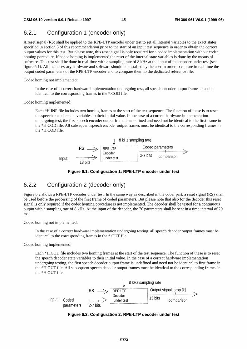
ETSI


6.2.1 Configuration 1 (encoder only)

A reset signal (RS) shall be applied to the RPE-LTP encoder under test to set all internal variables to the exact statesspecified in section 5 of this recommendation prior to the start of an input test sequence in order to obtain the correctoutput values for this test. But please note, this reset signal is only required for a codec implementation without codechoming porcedure. If codec homing is implemented the reset of the internal state variables is done by the means ofsoftware. This test shall be done in real-time with a sampling rate of 8 kHz at the input of the encoder under test (seefigure 6.1). All the necessary hardware and software should be installed by the user in order to capture in real time theoutput coded parameters of the RPE-LTP encoder and to compare them to the dedicated reference file.

Codec homing not implemented:

In the case of a correct hardware implementation undergoing test, all speech encoder output frames must beidentical to the corresponding frames in the *.COD file.

Codec homing implemented:

Each *H.INP file includes two homing frames at the start of the test sequence. The function of these is to resetthe speech encoder state variables to their initial value. In the case of a correct hardware implementationundergoing test, the first speech encoder output frame is undefined and need not be identical to the first frame inthe *H.COD file. All subsequent speech encoder output frames must be identical to the corresponding frames inthe *H.COD file.

v

//

8 kHz sampling rate

Coded parameters

2-7 bits

13 bits

RS

comparisonInput:

RPE-LTPEncoderunder test

Figure 6.1: Configuration 1: RPE-LTP encoder under test

6.2.2 Configuration 2 (decoder only)

Figure 6.2 shows a RPE-LTP decoder under test. In the same way as described in the coder part, a reset signal (RS) shallbe used before the processing of the first frame of coded parameters. But please note that also for the decoder this resetsignal is only required if the codec homing procedure is not implemented. The decoder shall be tested for a continuousoutput with a sampling rate of 8 kHz. At the input of the decoder, the 76 parameters shall be sent in a time interval of 20ms.

Codec homing not implemented:

In the case of a correct hardware implementation undergoing testing, all speech decoder output frames must beidentical to the corresponding frames in the *.OUT file.

Codec homing implemented:

Each *H.COD file includes two homing frames at the start of the test sequence. The function of these is to resetthe speech decoder state variables to their initial value. In the case of a correct hardware implementationundergoing testing, the first speech decoder output frame is undefined and need not be identical to first frame inthe *H.OUT file. All subsequent speech decoder output frames must be identical to the corresponding frames inthe *H.OUT file.

v

//

8 kHz sampling rate

Codedparameters 2-7 bits

13 bits

RS

comparisonInput:

RPE-LTPDecoderunder test

Output signal: srop [k]

Figure 6.2: Configuration 2: RPE-LTP decoder under test

ETSI


6.3 Test sequencesThe letter `H´ at the end of a file name denotes a test sequences with codec homing frames.

6.3.1 Test sequences for configuration 1

For configuration 1, four different input test sequence are provided:

SRQ01/SEQ01H Sequence for testing the overflow controls in the encoder;

SEQ02/SEQ02H Sequence for testing the LPC part of the encoder;

SEQ03/SEQ03H Sequence for testing the LTP part of the encoder;

SEQ04/SEQ04H Sequence for testing various critical parts of the algorithm.

Sequence SEQ01/SEQ01H uses a large number of saturated samples. The residual LPC signal reaches very high values,which has two effects on the processing:

- occurrence of a large number of overflows in addition/subtraction operations. Table 6.2 describes each overflowpoint and the number of occurrences for each.

- the excitation RPE samples have a large dynamic range and the 64 codewords of the sub-block maximum areeach obtained at least once on output.

Sequence SEQ02/SEQ02H focuses successively on each reflection coefficient calculated in the Schur recursion.Table 6.3 shows which frames deal with which reflection coefficient and its dynamic range. The Log.-Area codewordsoutput by the coder cover the full range of their possible values except the 2nd LARc that does not reach the value 0 and63 (min and max). The maximum value (63) is however obtained in sequence 4.

Sequence SEQ03/SEQ03H tests the long term predictor part of the algorithm. It has been generated by exciting asharply resonant filter with a periodic train of impulses; this produces a pitched signal. Each part corresponding to agiven pitch is 128 ms (4 blocks of 256 words) long. The pitch periods have been randomly drawn in the range [2,15] msand the random order is shown in table 6.4.

Sequence SEQ04/SEQ04H accounts for various remaining non tested points of the algorithm where implementing errorsmay be suspected. Tables 6.5 and 6.6 summarize the critical points that this sequence has been designed to check (i.e.where the three previous sequences were ineffective). Table 6.5 shows the list of tested points where errors can bedetected. Each tested error is described and the frame number corresponding to the first occurrence of a divergencebetween the exact and the degraded algorithm is also indicated.

Table 6.6 illustrates three paths of the algorithm that are never explored during the processing of the three previoussequences; the table shows which condition leads to each path and the number of associated occurrences in sequenceSEQ04/SEQ04H.

Notice finally one point where special care shall be taken:

- A small degradation (i.e. +/- 1) of DLB[2] (the third decision level of the LTP gain quantizer (see table 5.3a) isunable to provide any noticeable effect on the output of the four sequences described above).

6.3.2 Test sequences for configuration 2

Five different input test sequence are provided for this configuration. Four sequences obtained in configuration 1 at theoutput of the encoder (coded parameters) are used as input for the decoder under test in configuration 2.

Table 6.7 gives the list of tested overflow points and their occurrence on sequence SEQ01/SEQ01H for thisconfiguration.

Sequence SEQ05/SEQ05H is provided to scan all possible codes for each parameter. This sequence is an artificialsequence and does not correspond to any encoder output. The codewords have been randomly generated and cover theentire range of codewords values. Moreover, the delay value Nr belonging to [40,120] in an error-free transmissioncondition, takes in this sequence its value in [0,127]. In this case the decoder behaviour on non-allowed values of Nrwill be tested.

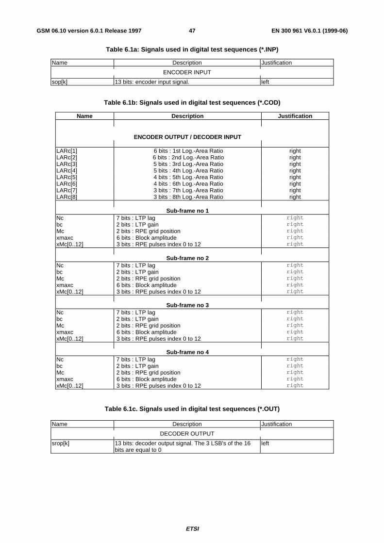
ETSI


Table 6.1a: Signals used in digital test sequences (*.INP)

Name Description Justification

ENCODER INPUT

sop[k] 13 bits: encoder input signal. left

Table 6.1b: Signals used in digital test sequences (*.COD)


ENCODER OUTPUT / DECODER INPUT

LARc[1] 6 bits : 1st Log.-Area Ratio rightLARc[2] 6 bits : 2nd Log.-Area Ratio rightLARc[3] 5 bits : 3rd Log.-Area Ratio rightLARc[4] 5 bits : 4th Log.-Area Ratio rightLARc[5] 4 bits : 5th Log.-Area Ratio rightLARc[6] 4 bits : 6th Log.-Area Ratio rightLARc[7] 3 bits : 7th Log.-Area Ratio rightLARc[8] 3 bits : 8th Log.-Area Ratio right

Sub-frame no 1Nc 7 bits : LTP lag rightbc 2 bits : LTP gain rightMc 2 bits : RPE grid position rightxmaxc 6 bits : Block amplitude rightxMc[0..12] 3 bits : RPE pulses index 0 to 12 right




Table 6.1c. Signals used in digital test sequences (*.OUT)


DECODER OUTPUT

srop[k] 13 bits: decoder output signal. The 3 LSB's of the 16bits are equal to 0

left

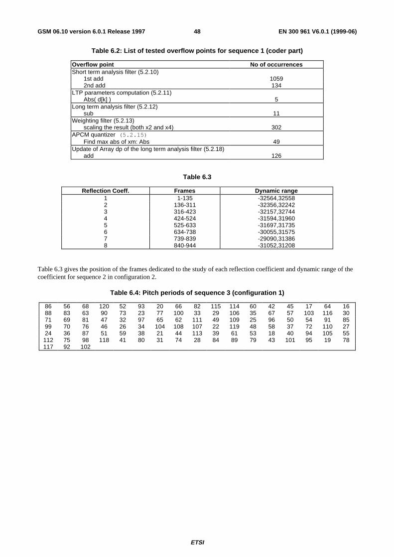
ETSI


Table 6.2: List of tested overflow points for sequence 1 (coder part)

Overflow point No of occurrencesShort term analysis filter (5.2.10) 1st add 1059 2nd add 134LTP parameters computation (5.2.11) Abs( d[k] ) 5Long term analysis filter (5.2.12) sub 11Weighting filter (5.2.13) scaling the result (both x2 and x4) 302APCM quantizer (5.2.15) Find max abs of xm: Abs 49Update of Array dp of the long term analysis filter (5.2.18) add 126

Table 6.3

Reflection Coeff. Frames Dynamic range1 1-135 -32564,325582 136-311 -32356,322423 316-423 -32157,327444 424-524 -31594,319605 525-633 -31697,317356 634-738 -30055,315757 739-839 -29090,313868 840-944 -31052,31208

Table 6.3 gives the position of the frames dedicated to the study of each reflection coefficient and dynamic range of thecoefficient for sequence 2 in configuration 2.

Table 6.4: Pitch periods of sequence 3 (configuration 1)

86 56 68 120 52 93 20 66 82 115 114 60 42 45 17 64 1688 83 63 90 73 23 77 100 33 29 106 35 67 57 103 116 3071 69 81 47 32 97 65 62 111 49 109 25 96 50 54 91 8599 70 76 46 26 34 104 108 107 22 119 48 58 37 72 110 2724 36 87 51 59 38 21 44 113 39 61 53 18 40 94 105 55

112 75 98 118 41 80 31 74 28 84 89 79 43 101 95 19 78117 92 102

ETSI


Table 6.5: Errors specially detected by sequence 4/Config 1

Error checked : No of theTest point incorrect / correct 1st frame

statement / statement with error

Autocorrelation function k=0 to 158/k=0 to 159 27 (5.2.4)

Computation of the reflect. if( P[0] <= / if( P[0] < 514 coefficients (5.2.5) abs(P[1]) ) / abs(P[1]) )

Quantization and coding A[4] + 1 /A[4] 21 of the LARs (5.2.7) A[5] - 1 /A[5] 35

A[5] + 1 /A[5] 430 A[6] - 1 /A[6] 427 A[8] - 1 /A[8] 8 MAC[2] - 1 / MAC[2] 24 MAC[2] + 1 / MAC[2] 516

Comput. of the rp from the 11058 / 11059 19 interp. LARp (5.2.9) 20069 / 20070 25

Calc. of the LTP parameters ->Search of the opt scaling k= 0 to 38 / k= 0 to 39 32 (5.2.11) ->Coding of the LTP gain mult_r/ mult 373 (5.2.11) DLB[0] + 1 / DLB[0] 511

DLB[1] + 1 / DLB[1] 373

ADPCM inverse quantizer FAC[2] + 1 / FAC[2] 422 (5.2.16) FAC[3] - 1 / FAC[3] 179

FAC[4] + 1 / FAC[4] 74 FAC[5] - 1 / FAC[5] 439 FAC[5] + 1 / FAC[5] 74 FAC[6] - 1 / FAC[6] 479 FAC[6] + 1 / FAC[6] 330 FAC[7] - 1 / FAC[7] 139

Table 6.6: Paths specially explored by sequence 4/Config 1

Test point Number of occurrences

Autocorrelation function (5.2.4) 8 condition smax == 0

Computation of the reflection coefficients : -> condition L_ACF[0] == 0 (5.2.5) 8 -> condition P[0] < abs(P[1])(5.2.5) 4

ETSI


Table 6.7: List of tested overflows points for sequence 1 (decoder part)

Overflow Point Nb of occurrencesSequence 1 Sequence 2 Sequence 3

Long term synthesis filter(5.3.2) : add 126 0 0

Short term synthesis filter :(5.3.4) 1st add: 4499 0 0 2nd add: 405 1 0

De-emphasize filter(5.3.5): add 89 0 0

Scaling of the output signal(5.3.6): add 16691 339 19

6.3.3 Additional Test sequences for Codec Homing

The test sequences decribed below are only required if the codec homing procedure is implemented.

6.3.3.1 Codec homing frames

In addition to the test sequences described above, two homing sequences are provided to assist in codec testing.SEQ06H.INP contains one encoder-homing-frame. SEQ06H.COD contains one decoder-homing-frame.

6.3.3.2 Sequence for an extensive test of the decoder homing

If the decoder receives a complete decoder-homing-frame (which is not marked as a bad frame), then it is suffient thatthe following frame contains only the LARs and the first subframe data of the decoder-homing-frame to cause a decoderreset and the output of the encoder-homing-frame. To check this behaviour the test sequence HOMING01.COD/OUTwas produced. As the test sequences SEQ01H...05H the sequence HOMING01 contains 2 complete decoder-homing-frames at the beginning and inside there is a mixture of complete and fractional (incomplete) decoder-homing-frames.

6.3.3.3 Sequences for finding the 20 ms framing of the GSM full rate speechencoder

When testing the decoder, alignment of the test sequences used to the decoder framing is achieved by the air interface(MS test) or can be reached easily on the Abis-interface (test on network side).

When testing the encoder, usually there is no information available about where the encoder starts its 20 ms segments ofspeech input to the encoder.

In the following, a procedure is described to find the 20 ms framing of the encoder using special synchronizationsequences. This procedure can be used for MS as well as for network side.

Synchronization can be achieved in two steps. First, bit synchronization has to be found. In a second step, framesynchronization can be determined. This procedure takes advantage of the codec homing feature of the full rate codec,which puts the codec in a defined home state after the reception of the first homing frame. On the reception of furtherhoming frames, the output of the codec is predefined which can be use as a trigger reference.

- Bit synchronization

The input to the speech encoder is a series of 13 bit long words (104 kbits/s, 13 bit linear PCM). When starting to testthe speech encoder, no knowledge is available of bit synchronization, i.e., where the encoder expects its least significantbits, and where it expects the most significant bits.

ETSI


The encoder-homing-frame consists of 160 samples, all set to zero with the exception of the least significant bit, whichis set to one (0 0000 0000 0001 binary, or 0x0008 hex if written into 16 bit words left justified). If two such encoder-homing-frames are input to the encoder consecutively, the decoder-homing-frame is expected at the output as a reactionof the second encoder-homing-frame.

Since there are only 13 possibilities for bit synchronization, after a maximum of 13 trials bit synchronization can bereached. In each0 trial three consecutive encoder-homing-frames are input to the encoder. If the decoder-homing-frameis not detected at the output, the relative bit position of the three input frames is shifted by one and another trial isperformed. As soon as the decoder-homing-frame is detected at the output, bit synchronization is found, and the firststep can be terminated.

The reason why three consecutive encoder-homing-frames are needed is that frame synchronization is not known at thisstage. To be sure that the encoder reads two complete homing frames, three frames have to be input. Wherever theencoder has its 20 ms segmentation, it will always read at least two complete encoder-homing-frames.

An example of the 13 different frame triplets is given in sequence BITSYNC.INP.

- Frame synchronization

Once bit synchronization is found, frame synchronization can be found by inputting one special frame that delivers 160different output frames, depending on the 160 different positions that this frame can possibly have with respect to theencoder framing.

This special synchronization frame was found by taking one input frame and shifting it through the positions 0 to 159.The corresponding 160 encoded speech frames were calculated and it was verified that all 160 output frames weredifferent. When shifting the input synchronization frame, the samples at the beginning were set to 0x0008 hex, whichcorresponds to the samples of the encoder-homing-frame.

Before inputting this special synchronization frame to the encoder, again the encoder has to be reset by one encoder-homing-frame. A second encoder-homing-frame is needed to provoke a decoder-homing-frame at the output that can beused as a trigger reference. Since the framing of the encoder is not known at that stage, three encoder-homing-frameshave to precede the special synchronization frame to ensure that the encoder reads at least two homing frames, and atleast one decoder-homing-frame is produced at the output, serving as a trigger for recording.

The special synchronization frame preceded by the three encoder-homing-frames are given in SEQSYNC.INP. Thecorresponding 160 different output frames are given in SYNC000.COD through SYNC159.COD. The three digitnumber in the filename indicates the number of samples by which the input is retarded with respect to the encoderframing. By a corresponding shift in the opposite direction, alignment with the encoder framing can be attained.

6.3.3.4 Formats and sizes of the synchronization sequences

BIT SYNC.INP:

This sequence consists of 13 frame triplets. It has the format of the speech encoder input test sequences (13 bit leftjustified with the three least significant bits set to zero).

The size of it is therefore:

SIZE (BITSYNC.INP) = 13 * 3 * 160 * 2 bytes = 12 480 bytes

SEQSYNC.INP:

This sequence consists of 3 encoder reset frames and the special synchronization frame. It has the format of the speechencoder input test sequences (13 bit left justified with the three least significant bits set to zero).

The size of it is therefore:

SIZE (SEQSYNC.INP) = 4 * 160 * 2 bytes = 1 280 bytes

SYNCXXX.COD:

These sequences consists of 1 encoder output frame each. They have the format of the speech encoder output testsequences (16 bit words right justified).

ETSI


The size of them is therefore:

SIZE (SYNCXXX.COD) = 76 * 2 bytes = 152 bytes

Optional 8 bit Test Sequences

In addition to the test sequences with and without homing as described above, two complete sets of test sequences withA-law and µ-law compressed are provided. These sequences allow the test of TRAU equipment by means of the A-Interface. On the A-Interface speech data is available as a 64 kbps PCM data stream of compressed samples with 8 bitseach.

The usage of these 8 bit test sequences is exactly the same as described above for the 13 bit linear test sequences exceptthat the A-Interface is used instead of feeding/taking them directly into/from the speech codec. Therefore bitsynchronization is not necessary, too.

Provided are the encoder input sequences _x.INP, the encoder output sequences _x.COD and the decoder outputsequences _x.OUT.

The _x.INP sequences are used at the encoder input and result in the _x.COD sequences at the encoder output.

The linear decoder input sequences .COD (without -x in their names) have to be used to force the 8 bit compresseddecoder output sequences -x.OUT.

The format of the _x.INP and _x.OUT sequences is such that 160 samples of a speech frame are contained in one byteeach. This results in a file size of half the size of the 13 bit linear test sequences

The format of the *.cod files remains unchanged.

ETSI


Annex A (informative):Codec performance

A.1 Performance of the RPE-LTP

A.1.1 IntroductionThe purpose of this annex is to give a broad outline of the performance of the RPE-LTP codec with other parts of thedigital network. Some general guidance is also offered on non-voice services.

A.1.2 Speech performancePlanning rules for digital processes are defined in terms of quantizing distortion units (qdu) which can be realized fromthe following formula (reference 1) using the assumption that the formula accuracy represents the determination of qdusfrom QN measurements:

QN = 37 - 15 log10(n) ,where n is the qdu (A1.1)

By definition 1 qdu is the quantization distortion arising from one commercial PCM codec.

NOTE: The subjective testing methodology to determine QN for the RPE-LTP codec was consistent with currentITU-T methods (reference 2).

A.1.2.1 Single encoding

Under error-free transmission conditions the perceived quality of the RPE-LTP codec (see figure A.1.1) is lower thanboth codecs conforming to recommendations ITU-T G.711 and ITU-T G.721 (superseded by G.726). Table A.1.1indicates the relative performance of the codec and can be compared with codecs conforming to recommendationsITU-T G.711 and ITU-T G.721 (superseded by G.726).

The performance of the RPE-LTP codec has been found to be substantially unaffected down to a carrier to interference(C/I) ratio of 10 dB, but may be considered to have acceptable performance down to 7 dB. Smaller C/I ratios produceunacceptable degradation of speech performance and should be avoided.

NOTE 1: It should be noted that there are doubts as to whether the simulations which generated the error patternproperly represent real operating conditions. The C/I values quoted should therefore only be considered asparameters of this simulation. They may not correspond to real radio interference conditions. Results fromearly GSM validation hardware show that the C/I values which give the performance quoted may beseveral dBs higher. Some error statistics of the simulations are shown in table A.1.2.

NOTE 2: The real condition C/I = 10 dB is believed to correspond to about 90 % coverage.

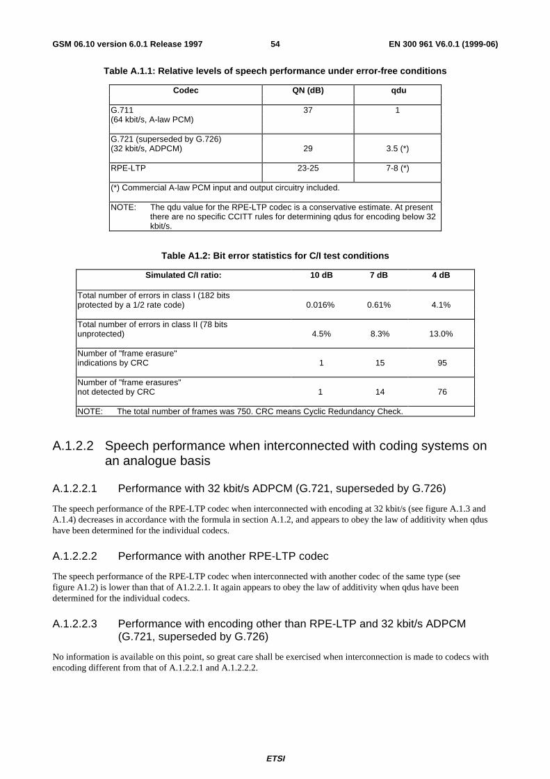
ETSI


Table A.1.1: Relative levels of speech performance under error-free conditions

Codec QN (dB) qdu

G.711 37 1(64 kbit/s, A-law PCM)

G.721 (superseded by G.726)(32 kbit/s, ADPCM) 29 3.5 (*)

RPE-LTP 23-25 7-8 (*)

(*) Commercial A-law PCM input and output circuitry included.

NOTE: The qdu value for the RPE-LTP codec is a conservative estimate. At presentthere are no specific CCITT rules for determining qdus for encoding below 32kbit/s.

Table A1.2: Bit error statistics for C/I test conditions

Simulated C/I ratio: 10 dB 7 dB 4 dB

Total number of errors in class I (182 bitsprotected by a 1/2 rate code) 0.016% 0.61% 4.1%

Total number of errors in class II (78 bitsunprotected) 4.5% 8.3% 13.0%

Number of "frame erasure"indications by CRC 1 15 95

Number of "frame erasures"not detected by CRC 1 14 76

NOTE: The total number of frames was 750. CRC means Cyclic Redundancy Check.

A.1.2.2 Speech performance when interconnected with coding systems onan analogue basis

A.1.2.2.1 Performance with 32 kbit/s ADPCM (G.721, superseded by G.726)

The speech performance of the RPE-LTP codec when interconnected with encoding at 32 kbit/s (see figure A.1.3 andA.1.4) decreases in accordance with the formula in section A.1.2, and appears to obey the law of additivity when qdushave been determined for the individual codecs.

A.1.2.2.2 Performance with another RPE-LTP codec

The speech performance of the RPE-LTP codec when interconnected with another codec of the same type (seefigure A1.2) is lower than that of A1.2.2.1. It again appears to obey the law of additivity when qdus have beendetermined for the individual codecs.

A.1.2.2.3 Performance with encoding other than RPE-LTP and 32 kbit/s ADPCM(G.721, superseded by G.726)

No information is available on this point, so great care shall be exercised when interconnection is made to codecs withencoding different from that of A.1.2.2.1 and A.1.2.2.2.

ETSI


A.1.3 Non-speech performanceIt should be noted that the RPE-LTP speech codec is an adaptive system which has been optimized for speech inputs.Great care shall be taken when making measurements with non-speech signals because the normal assumptions of timeinvariance and linearity cannot be made.

A.1.3.1 Performance with single sine waves

Detailed experiments have shown that the RPE-LTP codec will pass sine waves with segmental signal to noise ratiosgenerally in excess of 20 dB in the frequency range of 100 - 2000 Hz. However, in some cases reproduction above 2000Hz is not as good.

It should be noted that sine waves above 1300 Hz may be reproduced with significant fluctuations in amplitude andfrequency due to the adaptive sub-sampling technique employed. This results in irregularities in the measured frequencyresponse.

A typical frequency response measured with A-law PCM input circuitry is shown in figure A.1.5. If 13 bit linear PCMinput circuitry is used, the irregularity is less.

A.1.3.2 Performance with DTMF tones

It has been shown that the RPE-LTP codec transfers DTMF signals of 80 ms duration. However, questions likeminimum allowable signal duration, pause duration and the behaviour in the presence of transmission errors have notbeen investigated.

A.1.3.3 Performance with information tones

Experiments have shown that network originated signalling tones, conforming to recommendation ITU-T Q.35, areeasily recognizable when passed through the RPE-LTP codec.

A.1.3.4 Performance with voice-band data

Tests have shown that voice-band data transmission does not work satisfactorily with 1200 bit/s modems according torecommendation ITU-T V.23. Voice-band data according to recommendation ITU-T V.21 (300 bit/s) will not be subjectto any significant degradation.

This behaviour has been tested for one RPE-LTP link (encoder-decoder). The effect of transmission errors has not beentested.

A.1.4 DelayThe theoretical minimum delay of the RPE-LTP codec is 20 ms. However, practical realizations may have an additionalprocessing time in the order of 3 - 8 ms.

A/DA-law

encoderCodecRPE-LTP

A-lawdecoder

D/A

Figure A.1.1: One - transcoding scheme

ETSI


A/DA-law

encoderCodecRPE-LTP

A-lawdecoder

D/A

D/AA-law

decoderCodecRPE-LTP

A-lawencoder A/D

Figure A.1.2: Two - transcodings scheme

A/DA-law

encoderCodecRPE-LTP

A-lawdecoder

D/A

D/AA-law

decoderCodecG.721

A-lawencoder A/D

Figure A.1.3: Mixed transcodings - scheme 1

A/DA-law

encoderCodecG.721

A-lawdecoder

D/A

D/AA-law

decoderCodecRPE-LTP

A-lawencoder A/D

Figure A 1.4: Mixed transcodings - scheme 2

ETSI


Figure A.1.5: Frequency response for RPE-LTP codec(with commercial A-law PCM input and output circuitry)

A.1.5 Bibliography1) ITU-T: "Subjective performance assessment of digital processes using the Modulated Noise

Reference Unit (MNRU)", annex C, Supplement no 14, Red book, volume V, 1985.

2) ITU-T: "Subjective performance assessment of digital processes using the Modulated NoiseReference Unit (MNRU)", annex A, Supplement no 14, Red book, volume V, 1985.

3) ITU-T: "Technical characteristics of tones for the telephone service", recommendation Q.35, Redbook, volume VI.1, 1985.

A.2 Subjective relevance of the speech coder output bitsSince no valid objective quality criterion for speech signals is available, the only way to build up such a relevance tableis to perform listening tests. The procedure described below was used to obtain the relevance classification given intable A.2.1 of the recommendation.

To classify a single bit, say bit i of parameter k, a short speech signal (2 sec) was encoded, then this bit was inverted ineach frame (the other bits were left unchanged) and the resulting bit stream was fed into the speech decoder. Thelisteners had to compare the quality of the signal with the quality of six reference signals with different levels ofdistortion. Repeating this procedure for all bits would result in a subdivision of the 260 bits into six relevance classes. Itcan be observed that many of the bits have the same physical meaning and it can be expected that bits with the samemeaning have the same relevance (e.g. the MSB's of the RPE samples). Relying on this assumption, only one of theequivalent parameters was considered. Since there are 13 parameters with different physical meaning with 56 bits intotal, the number of tests is reduced from 260 to 56.

ETSI


The reference signals were the same speech signal distorted by inverting one of the six bits of LAR coefficient numberone. This resulted in an adequate quantization of distortion levels ranging from "not intelligible" (MSB inverted) to"negligible distortion" (LSB inverted).

The test was carried out using three listeners and one female speaker. Since the three listeners came to rather similarresults, no more listeners were considered to be required. Averaging the three outcomes led to the relevance table givenin table A.2.1, where the order of all bits between two successive bits of the first parameter (LAR 1) are arbitrarilychosen.

Table A.2.1a: Subjective importance of encoded bits(the parameter and bit numbers refer to table 1.1)

Importance Parameter Parameter Bit numberclass name number

1 Log.area ratio 1 1 b6Block amplitude 12,29,46,63 b53,b109,b165,b221

Log.area ratio 1 1 b52 Log.area ratio 2 2 b12

Log.area ratio 3 3 b17

Log.area ratio 1 1 b4Log.area ratio 2 2 b11Log.area ratio 3 3 b16Log.area ratio 4 4 b22LTP lag 9,26,43,60 b43,b99,b155,b211

3 Block amplitude 12,29,46,63 b52,b108,b164,b220Log.area ratio 2,5,6 2,5,6 b10,b26,b30LTP lag 9,26,43,60 b42,b98,b154,b210LTP lag 9,26,43,60 b41,b97,b153,b209LTP lag 9,26,43,60 b40,b96,b152,b208LTP lag 9,26,43,60 b39,b95,b151,b207

Block amplitude 12,29,46,63 b51,b107,b163,b219Log.area ratio 1 1 b3Log.area ratio 4 4 b21Log.area ratio 7 7 b33

4 LTP lag 9,26,43,60 b38,b94,b150,b206Log.area ratio 5,6 5,6 b25,b29LTP gain 10,27,44,61 b45,b101,b157,b213LTP lag 9,26,43,60 b37,b93,b149,b205Grid position 11,28,45,62 b47,b103,b159,b215

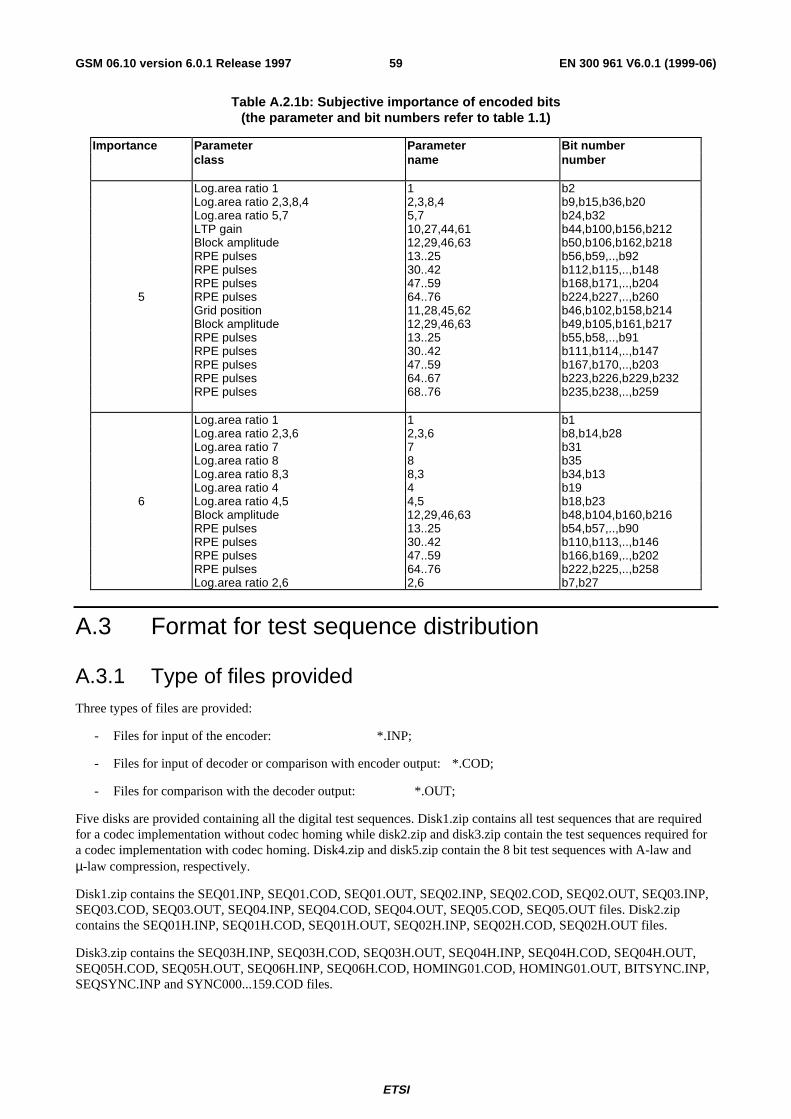
ETSI


Table A.2.1b: Subjective importance of encoded bits(the parameter and bit numbers refer to table 1.1)

Importance Parameter Parameter Bit numberclass name number

Log.area ratio 1 1 b2Log.area ratio 2,3,8,4 2,3,8,4 b9,b15,b36,b20Log.area ratio 5,7 5,7 b24,b32LTP gain 10,27,44,61 b44,b100,b156,b212Block amplitude 12,29,46,63 b50,b106,b162,b218RPE pulses 13..25 b56,b59,..,b92RPE pulses 30..42 b112,b115,..,b148RPE pulses 47..59 b168,b171,..,b204

5 RPE pulses 64..76 b224,b227,..,b260Grid position 11,28,45,62 b46,b102,b158,b214Block amplitude 12,29,46,63 b49,b105,b161,b217RPE pulses 13..25 b55,b58,..,b91RPE pulses 30..42 b111,b114,..,b147RPE pulses 47..59 b167,b170,..,b203RPE pulses 64..67 b223,b226,b229,b232RPE pulses 68..76 b235,b238,..,b259

Log.area ratio 1 1 b1Log.area ratio 2,3,6 2,3,6 b8,b14,b28Log.area ratio 7 7 b31Log.area ratio 8 8 b35Log.area ratio 8,3 8,3 b34,b13Log.area ratio 4 4 b19

6 Log.area ratio 4,5 4,5 b18,b23Block amplitude 12,29,46,63 b48,b104,b160,b216RPE pulses 13..25 b54,b57,..,b90RPE pulses 30..42 b110,b113,..,b146RPE pulses 47..59 b166,b169,..,b202RPE pulses 64..76 b222,b225,..,b258Log.area ratio 2,6 2,6 b7,b27

A.3 Format for test sequence distribution

A.3.1 Type of files providedThree types of files are provided:

- Files for input of the encoder: *.INP;

- Files for input of decoder or comparison with encoder output: *.COD;

- Files for comparison with the decoder output: *.OUT;

Five disks are provided containing all the digital test sequences. Disk1.zip contains all test sequences that are requiredfor a codec implementation without codec homing while disk2.zip and disk3.zip contain the test sequences required fora codec implementation with codec homing. Disk4.zip and disk5.zip contain the 8 bit test sequences with A-law andµ-law compression, respectively.

Disk1.zip contains the SEQ01.INP, SEQ01.COD, SEQ01.OUT, SEQ02.INP, SEQ02.COD, SEQ02.OUT, SEQ03.INP,SEQ03.COD, SEQ03.OUT, SEQ04.INP, SEQ04.COD, SEQ04.OUT, SEQ05.COD, SEQ05.OUT files. Disk2.zipcontains the SEQ01H.INP, SEQ01H.COD, SEQ01H.OUT, SEQ02H.INP, SEQ02H.COD, SEQ02H.OUT files.

Disk3.zip contains the SEQ03H.INP, SEQ03H.COD, SEQ03H.OUT, SEQ04H.INP, SEQ04H.COD, SEQ04H.OUT,SEQ05H.COD, SEQ05H.OUT, SEQ06H.INP, SEQ06H.COD, HOMING01.COD, HOMING01.OUT, BITSYNC.INP,SEQSYNC.INP and SYNC000...159.COD files.

ETSI


Disk4.zip contains the A-law compressed 8 bit test sequences with and without homing. All the files of disk1- 3.zipexcept for BITSYNC.INP, which is not necessary for TRAU testing, are on disk4.zip. The extension _A is added to thefilenames in order to indicate A-law. The files HOMING01, SEQSYC and SYNC000... are renamed to HOM01_A,SEQSYN_A and SYN000_A, respectively.

Disk5.zip contains the µ-law compressed 8 bit test sequences with and without homing similar to disk4.zip. The _u inthe filenames stands for µ-law.

Table A.3.1a/b gives the contents of the five disks and also the size in bytes and the number of frames for each testsequence file.

A.3.2 File format descriptionAll the files with the linear 13 bit test sequences are written in binary using 16 bit words. This means that input samples(sop[k], on files: *.INP), output samples (srop[k], on files: *.OUT) and coded parameters (on files: *.COD) use 2 byteseach. Hence the sizes of the files are directly related to the number of processed frames.

For files with linear 13 bit sequences and .INP or .OUT extension type:

Size (in bytes) = No of frames * 160 * 2;

All files _x.INP and _x.OUT with the compressed 8 bit test sequences are written in binary using 1 byte per sample.

For files with compressed 8 bit sequences and _x.INP or _x.OUT type:

Size (in bytes) = No of frames * 160 * ;

For all files with .COD extension type:

Size (in bytes) = No of frames * 76 * 2;

Table A.3.1 shows the size of all the 13 bit linear files written in direct binary format. The size of the files containing theoptional 8 bit test sequences with type _x.INP and _x.OUT is half the size shown in the table (disk4.zip and disk5.zip).

ETSI


Table A.3.1a: Contents of disk1.zip (test sequences without codec homing frames and file sizes)

DiskNo.

Purpose of Sequence Name of Sequence No. Of Frames Size in Bytes Justification

1/5 Codec test sequence SEQ01.INP 584 186 880 Left1/5 Codec test sequence SEQ01.COD 584 88 768 Right1/5 Codec test sequence SEQ01.OUT 584 186 880 Left1/5 Codec test sequence SEQ02.INP 947 303 040 Left1/5 Codec test sequence SEQ02.COD 947 143 944 Right1/5 Codec test sequence SEQ02.OUT 947 303 040 Left1/5 Codec test sequence SEQ03.INP 673 215 360 Left1/5 Codec test sequence SEQ03.COD 673 102 296 Right1/5 Codec test sequence SEQ03.OUT 673 215 360 Left1/5 Codec test sequence SEQ04.INP 520 166 400 Left1/5 Codec test sequence SEQ04.COD 520 79 040 Right1/5 Codec test sequence SEQ04.OUT 520 166 400 Left1/5 Decoder test sequence SEQ05.COD 64 9 728 Right1/5 Decoder test sequence SEQ05.OUT 64 20 480 Left

Table A.3.1b: Contents of disk2.zip and disk3.zip (test sequences with codec homing frames and filesizes)

DiskNo.

Purpose of Sequence Name of Sequence No. Of Frames Size in Bytes Justification

2/5 Codec test sequence SEQ01H.INP 586 187 520 Left2/5 Codec test sequence SEQ01H.COD 586 89 072 Right2/5 Codec test sequence SEQ01H.OUT 586 187 520 Left2/5 Codec test sequence SEQ02H.INP 949 303 680 Left2/5 Codec test sequence SEQ02H.COD 949 144 248 Right2/5 Codec test sequence SEQ02H.OUT 949 303 680 Left3/5 Codec test sequence SEQ03H.INP 675 216 000 Left3/5 Codec test sequence SEQ03H.COD 675 102 600 Right3/5 Codec test sequence SEQ03H.OUT 675 216 000 Left3/5 Codec test sequence SEQ04H.INP 522 167 040 Left3/5 Codec test sequence SEQ04H.COD 522 79 344 Right3/5 Codec test sequence SEQ04H.OUT 522 167 040 Left3/5 Decoder test sequence SEQ05H.COD 66 10 032 Right3/5 Decoder test sequence SEQ05H.OUT 66 21 120 Left3/5 Encoder-homing-frame SEQ06H.INP 1 320 Left3/5 Decoder-homing-frame SEQ06H.COD 1 152 Right3/5 Decoder homing test HOMING01.COD 100 15 200 Right3/5 Decoder homing test HOMING01.OUT 100 32 000 Left3/5 Bit Synchronization BITSYNC.INP 39 1 2480 Left3/5 Frame Synchronization (input) SEQSYNC.INP 4 1 280 Left3/53/53/5

""

3/5

Frame Synchronization (output) SYNC000.CODSYNC001.CODSYNC002.COD

"""

SYNC159.COD

111"""1

152152152

"""

152

RightRightRight

"""

Right

ETSI


Annex B (informative):Test sequence disksProvided in archive 8wc0300o.ZIP which accompanies the present document.

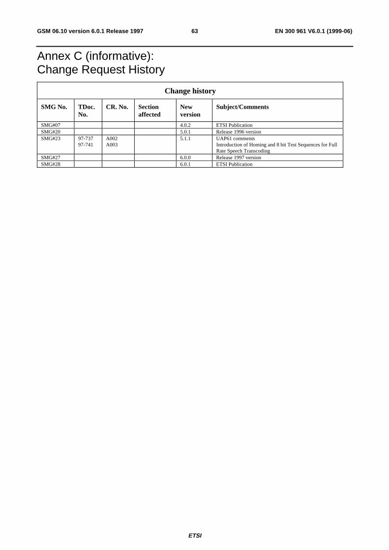
ETSI


Annex C (informative):Change Request History

Change history

SMG No. TDoc.No.

CR. No. Sectionaffected

Newversion

Subject/Comments

SMG#07 4.0.2 ETSI PublicationSMG#20 5.0.1 Release 1996 versionSMG#23 97-737

97-741A002A003

5.1.1 UAP61 commentsIntroduction of Homing and 8 bit Test Sequences for FullRate Speech Transcoding

SMG#27 6.0.0 Release 1997 versionSMG#28 6.0.1 ETSI Publication

ETSI


History

Document history

Edition 1 December 1996 Unified Approval Procedure UAP 61: 1996-12-16 to 1997-04-11

Edition 1 May 1997 Publication

Edition 2 December 1997 One-step Approval Procedure OAP 9817: 1997-12-26 to 1998-04-24

Edition 2 May 1998 Publication

V6.0.0 January 1999 One-step Approval Procedure OAP 9922: 1999-01-29 to 1999-05-28

V6.0.1 June 1999 Publication

ISBN 2-7437-2927-9Dépôt légal : Juin 1999

Documents

Full rate speech; Transcoding (GSM 06.10 version 6.0.1 … · 2000-02-02 · Full rate speech; Transcoding (GSM 06.10 version 6.0.1 Release 1997) GLOBAL SYSTEM FOR ... 3.1.7 Quantization