FULL PAPER Online Multi-Sensor Calibration Based on Moving

July 15, 2020 Advanced Robotics main

To appear in Advanced RoboticsVol. 35, No. 5, March 2021, 1–14

FULL PAPER

Online Multi-Sensor Calibration Based on Moving Object Tracking

J. Peršić∗, L. Petrović, I. Marković and I. Petrović

University of Zagreb, Faculty of Electrical Engineering and Computing,Laboratory for Autonomous Systems and Mobile Robotics (LAMOR)

(v1.0 released April 2020)

Modern autonomous systems often fuse information from many different sensors to enhance theirperception capabilities. For successful fusion, sensor calibration is necessary, while performing it onlineis crucial for long-term reliability. Contrary to currently common online approach of using ego-motionestimation, we propose an online calibration method based on detection and tracking of movingobjects. Our motivation comes from the practical perspective that many perception sensors of anautonomous system are part of the pipeline for detection and tracking of moving objects. Thus, byusing information already present in the system, our method provides resource inexpensive solutionfor the long-term reliability of the system. The method consists of a calibration-agnostic track totrack association, computationally lightweight decalibration detection, and a graph-based rotationcalibration. We tested the proposed method on a real-world dataset involving radar, lidar and camerasensors where it was able to detect decalibration after several seconds, while estimating rotation with0.2 error from a 20 s long scenario.

Keywords: multi-sensor calibration, online calibration, moving object tracking, radar, lidar, camera

1. Introduction

Modern robotic systems such as autonomous vehicles (AV) usually operate in highly dynamicscenarios where the actions they take significantly impact the surrounding environment. In orderto achieve autonomy, they have to reliably solve many complex tasks, such as environmentperception, motion prediction, motion planning and control. Environment perception, as the firstbuilding block of the autonomy pipeline, provides input data for many complex components, suchas simultaneous localization and mapping (SLAM), detection and tracking of moving objects(DATMO) and semantic scene understanding. To increase the accuracy and robustness of anautonomous system, environment perception is often based on fusion of information from multipleheterogeneous sensors, such as lidar, camera, radar, GNSS and IMU. Accurate sensor calibrationis a prerequisite for successful sensor fusion.The sensor calibration consists of finding the intrinsic, extrinsic and temporal parameters, i.e.

parameters of individual sensor models, transformations between sensor coordinate frames andalignment of sensor clocks, respectively. There are numerous offline and online approaches tosensor calibration and they vary significantly based on the sensors involved. While the offlineapproaches rely on controlled environments or calibration targets to achieve accurate calibration,the online approaches use information from the environment during the regular system operation,thus enabling long term robustness of the autonomous system. In this paper, we focus on theonline calibration methods which are applicable for lidar–camera–radar sensor systems.

∗Corresponding author. Email: [email protected]

1


The online calibration methods can be roughly divided into feature-based and motion-basedmethods. Feature-based methods rely on extracting informative structure from the environmentto generate correspondences between the sensors. These methods are limited to camera–lidar cal-ibration, since other existing sensors do not provide enough structural information. For instance,extrinsic camera–lidar calibration can be based on line features detected as intensity edges in theimage and depth discontinuities in the point cloud [1, 2]. Alternatively, the intensity of signalreturned by lidar was used in [3] to find extrinsic calibration by maximizing the mutual informa-tion between images from camera and projected intensity values measured by the lidar. Recently,Park et al. [4] proposed a method for extrinsic and temporal camera–lidar calibration based on3D point features in the environment. When the sensors do not provide enough structural infor-mation (e.g. radar), online calibration can be solved by depending on either the ego-motion ormotion of objects in the environment. The former come with the advantage that the sensors donot have to share a common field of view (FOV), while the latter also work with a static sensorsystems. In [5] authors proposed an ego-motion based calibration suitable for camera–lidar cali-bration, while Kellner et al. [6] proposed a solution for radar odometry and alignment with thethrust axis of the vehicle. Furthermore, Kummerle et al. [7] proposed simultaneous calibration,localization and mapping framework which enables both extrinsic calibration and estimation ofthe robot kinematic parameters. Recently, Giamou et al. [8] proposed a solution for globally opti-mal ego-motion based calibration. Tracking-based methods have mostly been employed in statichomogeneous sensor systems. To calibrate multiple stationary lidars, Quenzel et al. [9] relied ontracking of moving objects, while Glas et al. [10, 11] used human motion tracking. Human motionwas also used for a stationary camera calibration [12, 13]. Considering tracking-based calibrationof stationary heterogeneous sensors, Glas et al. [14] proposed a method for calibration of multi-ple 2D lidars and RGB-D cameras, while Schöller et al. [15] proposed a method for stationarycamera–radar calibration.Within the context of an AV, a sensor system consists of multiple lidars, cameras, radars

and other sensors. While it is sufficient to use only a subset of sensors for accurate ego-motionestimation, DATMO is often performed using all the available exteroceptive sensors to providea greater FOV coverage, robustness to adverse conditions and to increase the accuracy [16–18].Several datasets have been recently made public by both the industry and the academia toemphasize importance and accelerate research on DATMO [17, 19–21]. In this paper, we leveragecurrent state of the art in DATMO and propose an online calibration method based on it. Ourmotivation is to enable decalibration detection and recalibration based on the information whichis already present in an autonomous system pipeline without adding significant computationaloverhead. To the best of the authors’ knowledge, this is a first online calibration method thatis based on heterogeneous sensor DATMO on a moving platform. In addition, while severaltarget-based methods for calibration of radar–lidar–camera systems exists [22, 23], this is thefirst attempt to calibrate these sensors simultaneously in an online setting.Our method provides a full pipeline which includes: (i) DATMO algorithm for each sensor

modality, (ii) track-to-track association based on a calibration invariant measure, (iii) efficientdecalibration detection and (iv) a graph-based calibration handling multiple heterogeneous sen-sors simultaneously. We point out that our method estimates only rotational component of theextrinsic calibration, because translation is unobservable due to limited sensor accuracy and abias in detections (e.g. radar might measure a metal rear axle, while lidar detections report centerof a bounding box. Even the methods based on ego-motion would struggle estimating translationon an AV, because they require motion which excites at least two rotational axis [24]. How-ever, in contrast to rotational decalibration, feasible translational decalibration would not havea significant impact on the system performance. For instance, if rotational decalibration existed,object detection fusion would experience a growing error in the position with the increase inobject distance, while translational decalibration would only introduce a position error of equalvalue. Our method assumes that translational calibration is obtained using either target-basedor sensor-specific methods. The presented approach was evaluated on the nuScenes dataset [17],

2


Online calibration

Standard track fusion pipeline

Detection

Detection

Detection

Sensor 1Tracking

Tracking

Tracking

Track to trackassociation

Sensor 2

Sensor N

Decalibrationdetection

Graph-basedcalibration

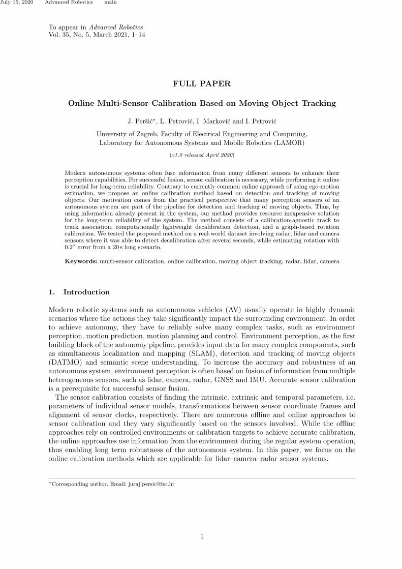
Figure 1. Illustration of the proposed pipeline for calibration based on DATMO. Detection, tracking and track to trackassociation are commonly parts of a track fusion pipelines. However, our association criterion is oriented towards beingcalibration agnostic. Thereafter, we propose two new modules: decalibration detection and graph-based calibration.

but is not in any way limited to this specific sensor setup. However, for testing our method, it iscurrently the only dataset containing appropriate data from cameras, radars and a lidar, whichare sensors in the focus of the proposed calibration method.

2. Proposed Method

In this section, we present each element of the method pipeline illustrated in Fig. 1. The pipelinestarts with the object detection which is specific for each sensor. Afterwards, the detections aretracked with separate trackers for each sensor which slightly differ among sensor modalities toaccommodate their specifics. The confirmed tracks of different sensors are then mutually associ-ated using calibration invariant measures. Each aforementioned stage has built-in outlier filteringmechanisms to prevent degradation of the results of subsequent steps. With the associated tracks,we proceed to a computationally lightweight decalibration detection. Finally, if decalibration isdetected, we proceed to the graph-based sensor calibration. The method handles asynchronoussensors by assuming temporal correspondence between sensor clocks is known and performinglinear interpolation of the object positions. Throughout the paper, we use the following notation:world frame Fw, ego-vehicle frame Fe and i-th sensor frame Fi. For convenience, we choose onesensor to be aligned with Fe. In the case of the nuScenes sensor setup, we chose the top lidar asit shares FOV segments with all the other sensors.

2.1 Object detection

The proposed pipeline starts with object detection performed for the each sensor individually.Automotive radars usually provide object detections obtained from proprietary algorithms per-formed locally on the sensor, while most can also provide tracked measurements. Obtaining theraw data is not possible due to low communication bandwidth of the CAN bus, typically used bythese sensors. Nevertheless, radars provide a list of detected objects consisting of the followingmeasured information: range, azimuth angle, range-rate, and radar cross-section (RCS). We usethese detections and classify them as moving or stationary based on the range-rate. Further-more, to avoid the need for extended target tracking where one target can generate multiplemeasurements, we perform clustering of close detections. These clusters are forwarded to theradar tracking module.Contrary to the radar, lidar’s and camera’s raw data provides substantial information from

which object detection is required. To extract detections from the lidar’s point cloud, we used the

3


MEGVII network based on sparse 3D convolution proposed by Zhu et al. [25] which is currentlythe best performing method for object detection on the nuScenes challenge. The method worksby accumulating 10 lidar sweeps into a single one to form a dense point cloud input, thus reducingthe effective frame rate of the sensor by a factor of 10. As the output, the network provides 3Dposition of objects as well as their size, orientation, velocity, class and detection score. Finally,for the object detection from images, we rely on a state-of-the-art 3D object detection approachdubbed CenterNet [26]. The output of CenterNet is similar to the lidar detections output, exceptthat the velocity information is not provided since detections are based on a single image. Weused the network weights trained on the KITTI dataset and determined the range scale factor bycomparing CenterNet detections to the MEGVII detections. At this stage, outlier filtering wasbased on the detection score threshold.

2.2 Tracking of moving objects

Tracking modules for individual sensors take detections from the previous step as inputs, asso-ciate them between different time frames and provide estimates of their states, which are laterused as inputs for subsequent steps. Since tracking is sensor specific, we perform it in each re-spective coordinate frame Fi. We adopt a similar single-hypothesis tracking strategy for all thesensors, following the nuScenes baseline approach [27]. Assigning detections to tracks is doneby using a global nearest neighbor approach and the Hungarian algorithm which provides effi-cient assignment solution [28]. The assignment is tuned by setting a threshold which controlsthe likelihood of a detection being assigned to a track. The state estimation of individual tracksis provided by an Extended Kalman filter which uses a constant turn-rate and velocity motionmodel [29]. Thus, the state vector in the lidar and camera tracker is

xk = [xk yk zk xk yk zk ωk]T , (1)

with the state transition defined as

xk+1 =

1 0 0 sin(ωkT )ωk

−1−cos(ωkT )ωk

0 0

0 1 0 1−cos(ωkT )ωk

sin(ωkT )ωk

0 0

0 0 1 0 0 T 00 0 0 cos (ωkT ) − sin (ωkT ) 0 00 0 0 sin (ωkT ) cos (ωkT ) 0 00 0 0 0 0 1 00 0 0 0 0 0 1

xk +

T 2

2 0 0 0

0 T 2

2 0 0

0 0 T 2

2 0T 0 0 00 T 0 00 0 T 00 0 0 1

w, (2)

where w = [wx wy wz wω]T is white noise on acceleration and turn-rate, while T is sensorsampling time. Using object position measurements forms the measurement model defined as

yk =

1 0 0 0 0 0 00 1 0 0 0 0 00 0 1 0 0 0 0

xk + v, (3)

where v = [vx vy vz]T is white measurement noise.

Due to the lack of radar’s elevation angle measurement, we drop the position and velocity inthe z-direction, thus reducing the state vector for the radar tracker to

xk = [xk yk xk yk ωk]T (4)

with adjusted state transition function and measurement model.

4


Track management is based on the track history, i.e. the track is confirmed after Nbirth consec-utive reliable detections and removed after Ncoast missing detections. All parameters are tunedfor each sensor separately as they have significantly different frame rates and accuracies. Lastly,subparts of individual tracks that exhibit sudden changes in velocity are marked as unreliableand these time instants are excluded from the subsequent steps.

2.3 Track-to-track association

Track to track association has been previously studied and a common approach is based on thehistory and distance of track positions [30]. Contrary to the traditional approaches, we do notassume a perfect calibration, as decalibration could degrade the association. Thus, we observetwo criteria for each track pair candidates through their common history: (i) mean of the velocitynorm difference and (ii) mean of the position norm difference. The track pair has to satisfy bothcriteria and not surpass predefined thresholds. If multiple associations are possible, none of themare associated. This conservative approach helps in eliminating wrong association which wouldcompromise the following calibration steps. However, the remaining tracks can be associated withmore common association metrics (e.g. Euclidean or Mahalanobis distance) and used within atrack fusion module. In our method we can use such a conservative approach and discard sometrack associations, since our goal is sensor calibration and not safety critical online DATMO forvehicle navigation.The position norm is not truly calibration independent, as it is affected by both the measure-

ment bias in the individual sensor and the translation between the sensors. Thus we use it ina loose way solely to distinguish between clearly distant tracks, i.e. we rely on the previouslycalibrated translational parameters and use a high threshold. On the other hand, velocity normhas already been used in a stationary system calibration for track association [14] as well as forframe-invariant temporal calibration of the sensors [31]. In a stationary scenario, it is trivial thatvelocity norm measured from different reference frames is equal. However, with a moving sensorplatform which experiences both translational and rotational movement, this insight may notbe that trivial. Namely, if a rigid body has non-zero angular velocity, different points on it willexperience different translational velocities due to the lever arm. To state this more formally, wepresent the following proposition

Proposition 1. Translational velocity norm of moving objects estimated from two referenceframes F1 and F2 on the same rigid body is invariant to the transform between the frames andthe motion of the rigid body.

Proof. Let wpk be the position of the observed object at time k in the Fw. Then, let 1pk and2pk be the same position expressed in the sensor reference frames F1 and F2, respectively:

1pk = 1wRk · wpk + 1

wtk, (5)

2pk = 21R · 1pk + 2

1t, (6)

where we express the motion of the rigid body (1wRk,1wtk) as time-varying SE(3) transform,

while the transform between sensors frames (i.e. calibration) is constant in time (21R,21t). Let us

now observe displacement of the moving object in the two sensor frames, 1δp and 2δp, betweentwo discrete time instances k and l:

1δp = 1pk − 1pl, (7)

2δp = 2pk − 2pl = 21R(1pk − 1pl) = 2

1R1δp. (8)

5


Since the rotation matrix is orthogonal, the norm of displacement is equal, i.e. ||2δp|| =||21R1δp|| = ||1δp||. Thus, the translational velocity norm is also equal because it is simplythe ratio of the above displacements over the time difference k − l.

2.4 Decalibration detection

In a standard track fusion pipeline, track associations from the previous step are commonly usedin object state estimate fusion. However, fusion depends on the accuracy of sensor calibrationwhich can change over time due to disturbances. Thus, we propose a computationally inexpen-sive decalibration detection method, which is based on the data already present in the system.Similarly to the strategy presented by Deray et al. [32], we adopt a window-based approach fordecalibration detection, but tailor the criterion we observe to accommodate the tracking-basedscenario.At the time instant tk we form sets of corresponding track positions i,jSw = (exi,

exj) that fallwithin the time window of length Tw (t ∈ (tk − Tw, tk)) for each sensor pair, where exi and exj

represent stacked object positions obtained by i-th and j-th sensor, respectively. The positions aretransformed from individual sensor frames Fi and Fj into the common reference frame Fe usingthe current calibration parameters. In the ideal case, the position should coincide, but due to theinevitable bias in the sensor measurements and the decalibration, in practice the error is alwaysnon-zero. To distinguish the error caused by bias from the decalibration error, we use an efficientclosed-form solution for orthogonal Procrustes problem to obtain pairwise sensor calibrations [33].Based on the i,jSw, we form a 3× 3 data matrix:

H = (exi − exi)(exj − exj)

T , (9)

where exi and exj are means of corresponding sets. The rotation jiR can be found using the

singular-value decomposition (SVD):

[U, S, V ] = SVD(H), (10)

jiR = V UT . (11)

Since the jiR should be an identity matrix in the ideal case, we define the decalibration criterion

for the time instant tk as an angle of rotation in the angle-axis representation by

Jk = arccos

(Tr(jiR)− 1

2

). (12)

When the criterion (12) surpasses a predefined threshold, the system proceeds to the completegraph-based sensor calibration. The magnitude of the minimal decalibration that can be detectedis limited by the predefined threshold and the horizon defined with the Tw. Longer horizon enablesdetection of smaller calibration changes, but with slower convergence.

2.5 Graph-based extrinsic calibration

The last step of the pipeline estimates the extrinsic parameters when the system detects decal-ibration. As previously mentioned, we handle only rotational decalibration due to the limitedaccuracy and the bias in the measurements. Since we are dealing with more than two sensors,pairwise calibration would produce inconsistent transformations among the sensors. Thus, we rely

6


−20 0 20 40 60 80 100 120 140

−5

0

5

x [m]

y[m

]

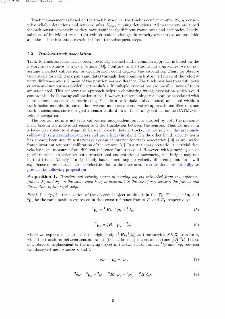
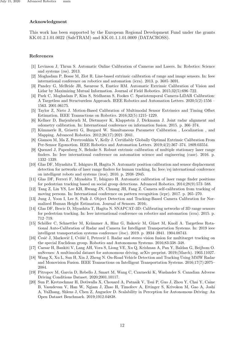
Figure 2. Illustration of the used scene showing ego-vehicle trajectory (red), lidar detections at t = 19s (blue) and historyof lidar tracks (yellow).

on the graph-based optimization presented in [34]. However, to ensure and speed up the conver-gence, we use the results of the previous step as an initialization. In the graph-based multi-sensorcalibration paradigm, one sensor is chosen as an anchor and aligned with the Fe for convenience.We then search for the poses of other sensors with respect to the anchor sensor by minimizingthe following criterion:

φ = arg minφ

i 6=j∑i,j

Nij∑k=1

eTi,j,k ·Ωi,j,k · ei,j,k (13)

ei,j,k = ipi,k − (ijR(φ)jpj,k + itj) (14)

where φ is a set of non-anchor sensor rotation parametrizations and Nij is the number of corre-sponding measurements between the i− th and j − th sensor. To enable integration of the noisefrom both sensors, we follow the total least squares approach presented in [35] and define thenoise model as:

Ωi,j,k = (ijR(φ)V [jpj,k]ijRT (φ) + V [ipi,k])−1 (15)

where V [·] is an observation covariance matrix of the zero-mean Gaussian noise. Additionally,if a sensor does not have a direct link with the anchor sensor, we obtain i

jR by multiplying thecorresponding series of rotation matrices to obtain the final rotation between the i-th and j-thsensor. This approach enables the estimation of all parameters with a single optimization, whileensuring consistency between sensor transforms.

3. Experimental Results

To validate the proposed method we used real world data provided with the nuScenes dataset[17]. Important details on the dataset, sensor setup and the scenario are given in Sec. 3.1, whileSec. 3.2 presents the results for each step of the calibration pipeline with greater attention onthe introduced novelties related to calibration (Sec. 2.3 - 2.5).

3.1 Experimental setup

The nuScenes dataset consists of 1000 scenes that are 20 s long and collected with a vehicledriven through Boston and Singapore. The vehicle is equipped with a roof-mounted 3D lidar, 5radars and 6 cameras. Each sensor modality has 360 coverage with small overlap of the sensors

7


(a) Lidar

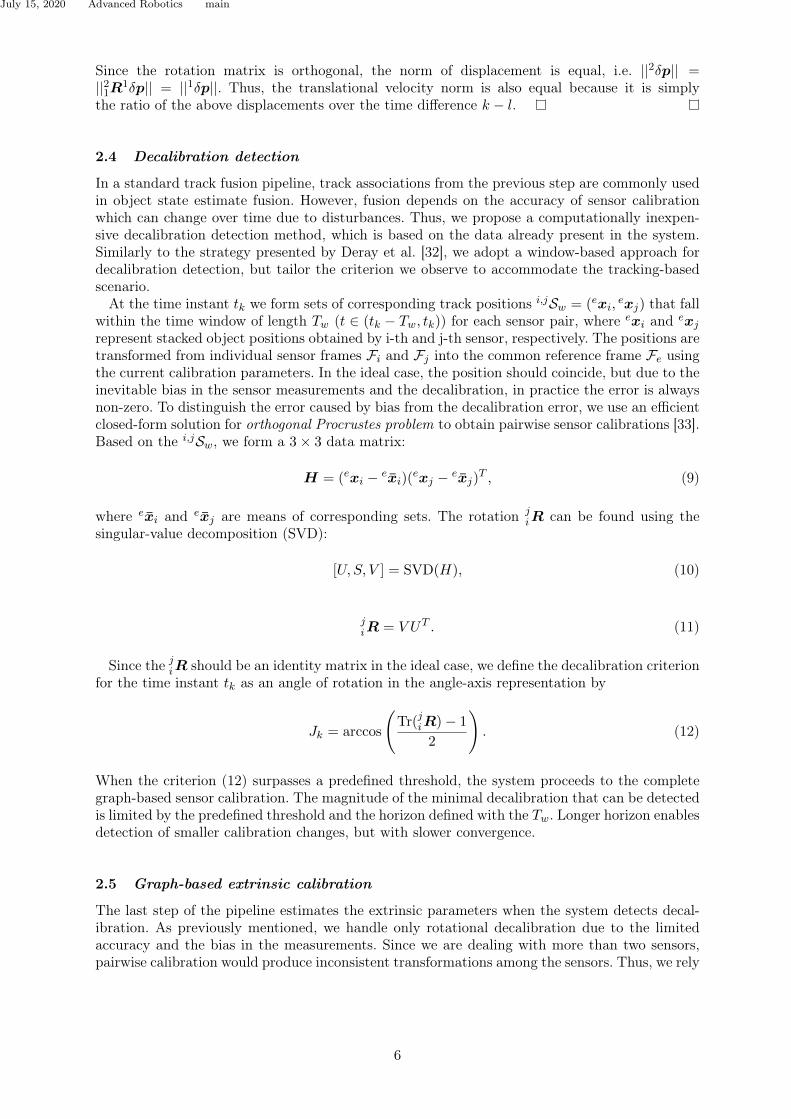
(b) Camera (c) Radar

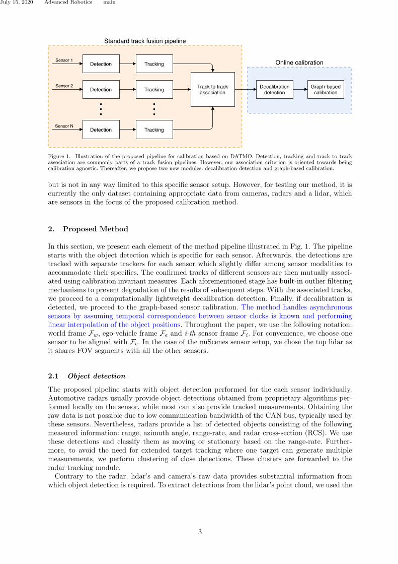
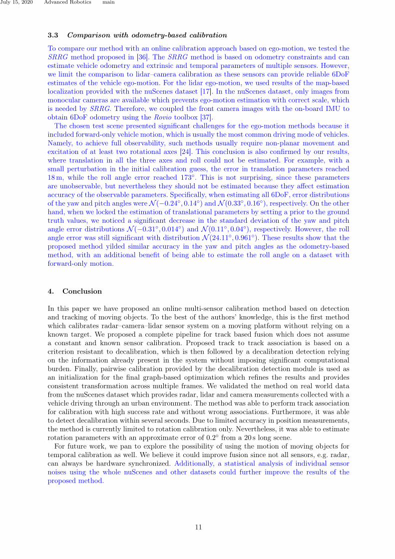
Figure 3. Vehicle detection using lidar, camera and radar. Lidar pointcloud consists of 10 consecutive sweeps, while blueand green boxes represent car and truck detections, respectively. Radar detections are colored with radar cross-section andshow range rate, while gray circles represent confirmed tracks.

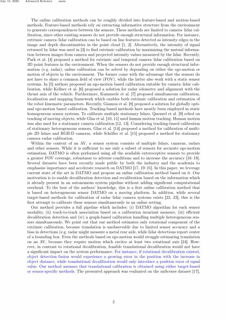
within the same modality. For clarity, in this experiment we focus only on measurements fromthe top lidar, front radar and front camera which all share a common FOV. The radar works at13Hz, camera 12Hz, while the lidar provides point clouds with 20Hz with the effective framerate reduced to 2Hz due to the object detector. The intrinsic and extrinsic calibration of allthe sensors is obtained using several methods and calibration targets and is provided with thedataset. We considered it as a ground truth in the assessment of our method. Furthermore, weused isotropic and identical noise models for all the sensors involved.In the following section, we present the results for scene 343 from the dataset, because it

contains variety of motions (cf. Fig. 2). The scene is from the test subpart of the dataset forwhich the data annotations are not provided. The ego vehicle is stationary during the first 5 s,while afterward it accelerates and reaches a speed of around 40 km/h. Through the scene, totalof 17 moving vehicles are driving in both the same and the opposite direction, while some ofthem make turns. In addition, the scene contains 8 stationary vehicles in the detectable area forall the sensors.

3.2 Results

We present the results sequentially for all the steps of the method as they progress through thepipeline illustrated in Fig. 1. The starting point of the pipeline is object detection using individualsensors illustrated by Fig. 3. Object detection using lidar and camera provided reliable resultsfor the range of up to 50m, both for moving and stationary vehicles. Rare false negatives didnot cause significant challenges for the subsequent steps. In comparison to the camera, lidarprovided significantly more detections with frequent false positives which we successfully filteredby setting a threshold on their detection scores. In addition, Fig. 3(a) illustrates how the MEGVII

8


0 5 10 15 20

0

1

2

3

tk [s]

Jk[]

L–RR–CL–C

(a) Without decalibration

0 5 10 15 20

0

1

2

3

tk [s]

Jk[]

L–RR–CL–C

(b) Decalibration at tk = 5

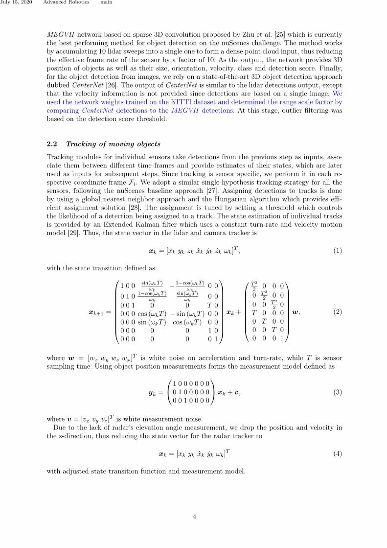
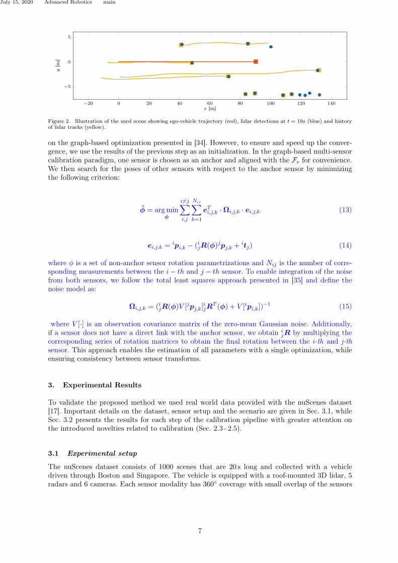
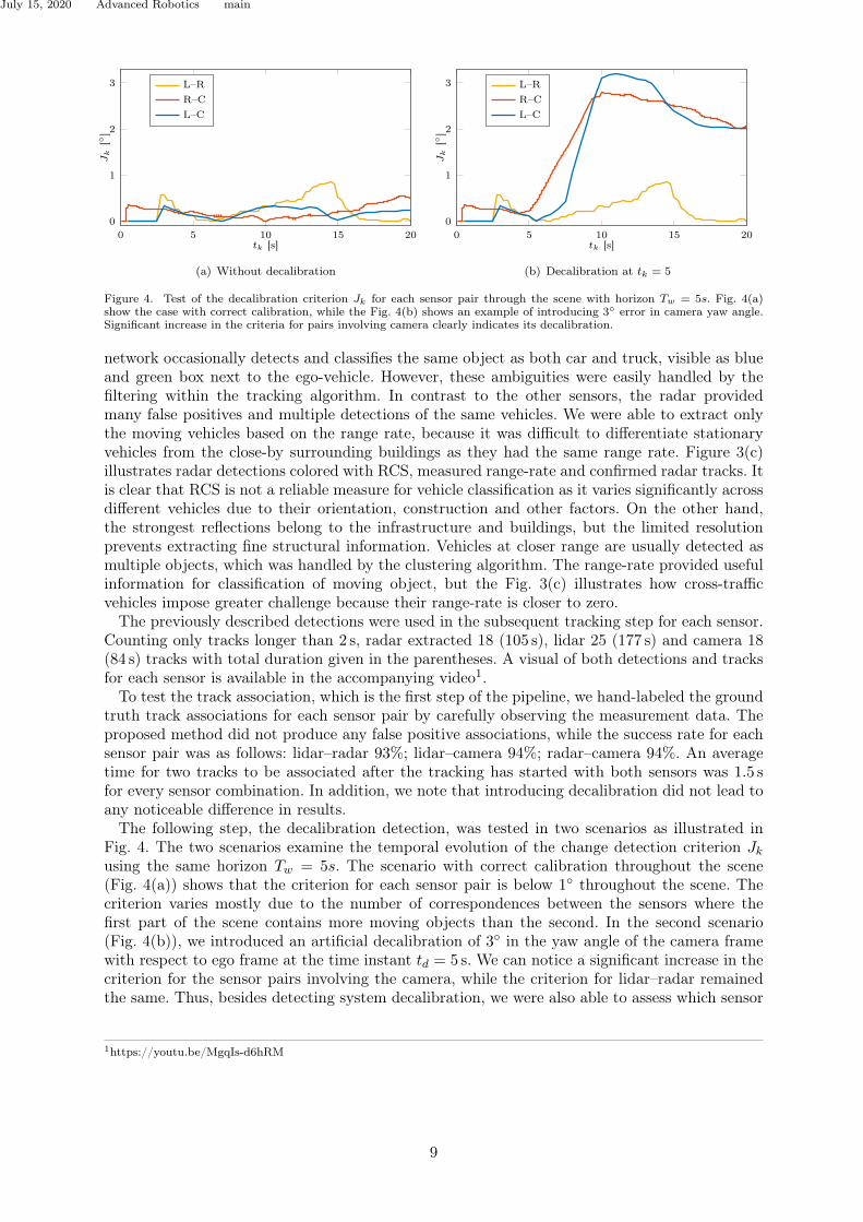
Figure 4. Test of the decalibration criterion Jk for each sensor pair through the scene with horizon Tw = 5s. Fig. 4(a)show the case with correct calibration, while the Fig. 4(b) shows an example of introducing 3 error in camera yaw angle.Significant increase in the criteria for pairs involving camera clearly indicates its decalibration.

network occasionally detects and classifies the same object as both car and truck, visible as blueand green box next to the ego-vehicle. However, these ambiguities were easily handled by thefiltering within the tracking algorithm. In contrast to the other sensors, the radar providedmany false positives and multiple detections of the same vehicles. We were able to extract onlythe moving vehicles based on the range rate, because it was difficult to differentiate stationaryvehicles from the close-by surrounding buildings as they had the same range rate. Figure 3(c)illustrates radar detections colored with RCS, measured range-rate and confirmed radar tracks. Itis clear that RCS is not a reliable measure for vehicle classification as it varies significantly acrossdifferent vehicles due to their orientation, construction and other factors. On the other hand,the strongest reflections belong to the infrastructure and buildings, but the limited resolutionprevents extracting fine structural information. Vehicles at closer range are usually detected asmultiple objects, which was handled by the clustering algorithm. The range-rate provided usefulinformation for classification of moving object, but the Fig. 3(c) illustrates how cross-trafficvehicles impose greater challenge because their range-rate is closer to zero.The previously described detections were used in the subsequent tracking step for each sensor.

Counting only tracks longer than 2 s, radar extracted 18 (105 s), lidar 25 (177 s) and camera 18(84 s) tracks with total duration given in the parentheses. A visual of both detections and tracksfor each sensor is available in the accompanying video1.To test the track association, which is the first step of the pipeline, we hand-labeled the ground

truth track associations for each sensor pair by carefully observing the measurement data. Theproposed method did not produce any false positive associations, while the success rate for eachsensor pair was as follows: lidar–radar 93%; lidar–camera 94%; radar–camera 94%. An averagetime for two tracks to be associated after the tracking has started with both sensors was 1.5 sfor every sensor combination. In addition, we note that introducing decalibration did not lead toany noticeable difference in results.The following step, the decalibration detection, was tested in two scenarios as illustrated in

Fig. 4. The two scenarios examine the temporal evolution of the change detection criterion Jkusing the same horizon Tw = 5s. The scenario with correct calibration throughout the scene(Fig. 4(a)) shows that the criterion for each sensor pair is below 1 throughout the scene. Thecriterion varies mostly due to the number of correspondences between the sensors where thefirst part of the scene contains more moving objects than the second. In the second scenario(Fig. 4(b)), we introduced an artificial decalibration of 3 in the yaw angle of the camera framewith respect to ego frame at the time instant td = 5 s. We can notice a significant increase in thecriterion for the sensor pairs involving the camera, while the criterion for lidar–radar remainedthe same. Thus, besides detecting system decalibration, we were also able to assess which sensor

1https://youtu.be/MgqIs-d6hRM

9


0 2 4 6 8 10 12 14 16 18 20

−0.2

0

0.2

0.4∆θz[]

Radar-Lidar

Yaw

0 2 4 6 8 10 12 14 16 18 20−1

−0.5

0

0.5

1

∆θz[]

Radar-Camera

Yaw

0 2 4 6 8 10 12 14 16 18 20−0.5

0

0.5

1

1.5

t [s]

∆θ[]

Lidar-Camera

YawPitchRoll

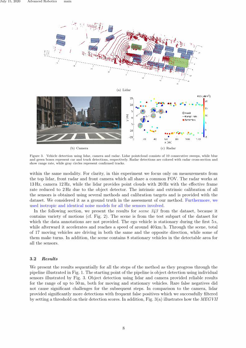
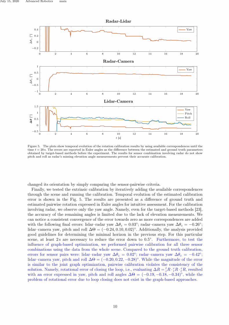
Figure 5. The plots show temporal evolution of the rotation calibration results by using available correspondences until thetime t = 20 s. The errors are reported in Euler angles as the difference between the estimated and ground truth parametersobtained by target-based methods before the experiment. The results for sensor combination involving radar do not showpitch and roll as radar’s missing elevation angle measurements prevent their accurate calibration.

changed its orientation by simply comparing the sensor-pairwise criteria.Finally, we tested the extrinsic calibration by iteratively adding the available correspondences

through the scene and running the calibration. Temporal evolution of the estimated calibrationerror is shown in the Fig. 5. The results are presented as a difference of ground truth andestimated pairwise rotation expressed in Euler angles for intuitive assessment. For the calibrationinvolving radar, we observe only the yaw angle. Namely, even for the target-based methods [23],the accuracy of the remaining angles is limited due to the lack of elevation measurements. Wecan notice a consistent convergence of the error towards zero as more correspondences are addedwith the following final errors: lidar–radar yaw ∆θz = 0.03; radar–camera yaw ∆θz = −0.26;lidar–camera yaw, pitch and roll ∆Θ = (−0.24, 0.10, 0.02). Additionally, the analysis providedgood guidelines for determining the minimal horizon in the previous step. For this particularscene, at least 2 s are necessary to reduce the error down to 0.5. Furthermore, to test theinfluence of graph-based optimization, we performed pairwise calibration for all three sensorcombinations using the data from the whole scene. Compared to the ground truth calibration,errors for sensor pairs were: lidar–radar yaw ∆θz = 0.02; radar–camera yaw ∆θz = −0.42;lidar–camera yaw, pitch and roll ∆Θ = (−0.20, 0.22,−0.28). While the magnitude of the erroris similar to the joint graph optimization, pairwise calibration violates the consistency of thesolution. Namely, rotational error of closing the loop, i.e., evaluating ∆R = l

cR · crR · rlR, resultedwith an error expressed in yaw, pitch and roll angles ∆Θ = (−0.19,−0.18,−0.34), while theproblem of rotational error due to loop closing does not exist in the graph-based approaches.

10


3.3 Comparison with odometry-based calibration

To compare our method with an online calibration approach based on ego-motion, we tested theSRRG method proposed in [36]. The SRRG method is based on odometry constraints and canestimate vehicle odometry and extrinsic and temporal parameters of multiple sensors. However,we limit the comparison to lidar–camera calibration as these sensors can provide reliable 6DoFestimates of the vehicle ego-motion. For the lidar ego-motion, we used results of the map-basedlocalization provided with the nuScenes dataset [17]. In the nuScenes dataset, only images frommonocular cameras are available which prevents ego-motion estimation with correct scale, whichis needed by SRRG. Therefore, we coupled the front camera images with the on-board IMU toobtain 6DoF odometry using the Rovio toolbox [37].The chosen test scene presented significant challenges for the ego-motion methods because it

included forward-only vehicle motion, which is usually the most common driving mode of vehicles.Namely, to achieve full observability, such methods usually require non-planar movement andexcitation of at least two rotational axes [24]. This conclusion is also confirmed by our results,where translation in all the three axes and roll could not be estimated. For example, with asmall perturbation in the initial calibration guess, the error in translation parameters reached18m, while the roll angle error reached 173. This is not surprising, since these parametersare unobservable, but nevertheless they should not be estimated because they affect estimationaccuracy of the observable parameters. Specifically, when estimating all 6DoF, error distributionsof the yaw and pitch angles were N (−0.24, 0.14) and N (0.33, 0.16), respectively. On the otherhand, when we locked the estimation of translational parameters by setting a prior to the groundtruth values, we noticed a significant decrease in the standard deviation of the yaw and pitchangle error distributions N (−0.31, 0.014) and N (0.11, 0.04), respectively. However, the rollangle error was still significant with distribution N (24.11, 0.961). These results show that theproposed method yilded similar accuracy in the yaw and pitch angles as the odometry-basedmethod, with an additional benefit of being able to estimate the roll angle on a dataset withforward-only motion.

4. Conclusion

In this paper we have proposed an online multi-sensor calibration method based on detectionand tracking of moving objects. To the best of the authors’ knowledge, this is the first methodwhich calibrates radar–camera–lidar sensor system on a moving platform without relying on aknown target. We proposed a complete pipeline for track based fusion which does not assumea constant and known sensor calibration. Proposed track to track association is based on acriterion resistant to decalibration, which is then followed by a decalibration detection relyingon the information already present in the system without imposing significant computationalburden. Finally, pairwise calibration provided by the decalibration detection module is used asan initialization for the final graph-based optimization which refines the results and providesconsistent transformation across multiple frames. We validated the method on real world datafrom the nuScenes dataset which provides radar, lidar and camera measurements collected with avehicle driving through an urban environment. The method was able to perform track associationfor calibration with high success rate and without wrong associations. Furthermore, it was ableto detect decalibration within several seconds. Due to limited accuracy in position measurements,the method is currently limited to rotation calibration only. Nevertheless, it was able to estimaterotation parameters with an approximate error of 0.2 from a 20 s long scene.For future work, we pan to explore the possibility of using the motion of moving objects for

temporal calibration as well. We believe it could improve fusion since not all sensors, e.g. radar,can always be hardware synchronized. Additionally, a statistical analysis of individual sensornoises using the whole nuScenes and other datasets could further improve the results of theproposed method.

11


Acknowledgment

This work has been supported by the European Regional Development Fund under the grantsKK.01.2.1.01.0022 (SafeTRAM) and KK.01.1.1.01.0009 (DATACROSS).

References

[1] Levinson J, Thrun S. Automatic Online Calibration of Cameras and Lasers. In: Robotics: Scienceand systems (rss). 2013.

[2] Moghadam P, Bosse M, Zlot R. Line-based extrinsic calibration of range and image sensors. In: Ieeeinternational conference on robotics and automation (icra). 2013. p. 3685–3691.

[3] Pandey G, McBride JR, Savarese S, Eustice RM. Automatic Extrinsic Calibration of Vision andLidar by Maximizing Mutual Information. Journal of Field Robotics. 2015;32(5):696–722.

[4] Park C, Moghadam P, Kim S, Sridharan S, Fookes C. Spatiotemporal Camera-LiDAR Calibration:A Targetless and Structureless Approach. IEEE Robotics and Automation Letters. 2020;5(2):1556 –1563. 2001.06175.

[5] Taylor Z, Nieto J. Motion-Based Calibration of Multimodal Sensor Extrinsics and Timing OffsetEstimation. IEEE Transactions on Robotics. 2016;32(5):1215–1229.

[6] Kellner D, Barjenbruch M, Dietmayer K, Klappstein J, Dickmann J. Joint radar alignment andodometry calibration. In: International conference on information fusion. 2015. p. 366–374.

[7] Kümmerle R, Grisetti G, Burgard W. Simultaneous Parameter Calibration , Localization , andMapping. Advanced Robotics. 2012;26(17):2021–2041.

[8] Giamou M, Ma Z, Peretroukhin V, Kelly J. Certifiably Globally Optimal Extrinsic Calibration FromPer-Sensor Egomotion. IEEE Robotics and Automation Letters. 2019;4(2):367–374. 1809.03554.

[9] Quenzel J, Papenberg N, Behnke S. Robust extrinsic calibration of multiple stationary laser rangefinders. In: Ieee international conference on automation science and engineering (case). 2016. p.1332–1339.

[10] Glas DF, Miyashita T, Ishiguro H, Hagita N. Automatic position calibration and sensor displacementdetection for networks of laser range finders for human tracking. In: Ieee/rsj international conferenceon intelligent robots and systems (iros). 2010. p. 2938–2945.

[11] Glas DF, Ferreri F, Miyashita T, Ishiguro H. Automatic calibration of laser range finder positionsfor pedestrian tracking based on social group detections. Advanced Robotics. 2014;28(9):573–588.

[12] Tang Z, Lin YS, Lee KH, Hwang JN, Chuang JH, Fang Z. Camera self-calibration from tracking ofmoving persons. In: International conference on pattern recognition (icpr). 2017. p. 265–270.

[13] Jung J, Yoon I, Lee S, Paik J. Object Detection and Tracking-Based Camera Calibration for Nor-malized Human Height Estimation. Journal of Sensors. 2016;.

[14] Glas DF, Brscic D, Miyashita T, Hagita N. SNAPCAT-3D: Calibrating networks of 3D range sensorsfor pedestrian tracking. In: Ieee international conference on robotics and automation (icra). 2015. p.712–719.

[15] Schöller C, Schnettler M, Krämmer A, Hinz G, Bakovic M, Güzet M, Knoll A. Targetless Rota-tional Auto-Calibration of Radar and Camera for Intelligent Transportation Systems. In: 2019 ieeeintelligent transportation systems conference (itsc). 2019. p. 3934–3941. 1904.08743.

[16] Ćesić J, Marković I, Cvišić I, Petrović I. Radar and stereo vision fusion for multitarget tracking onthe special Euclidean group. Robotics and Autonomous Systems. 2016;83:338–348.

[17] Caesar H, Bankiti V, Lang AH, Vora S, Liong VE, Xu Q, Krishnan A, Pan Y, Baldan G, Beijbom O.nuScenes: A multimodal dataset for autonomous driving. arXiv preprint. 2019;(March). 1903.11027.

[18] Wang X, Xu L, Sun H, Xin J, Zheng N. On-Road Vehicle Detection and Tracking Using MMW Radarand Monovision Fusion. IEEE Transactions on Intelligent Transportation Systems. 2016;17(7):2075–2084.

[19] Pitropov M, Garcia D, Rebello J, Smart M, Wang C, Czarnecki K, Waslander S. Canadian AdverseDriving Conditions Dataset. 2020;2001.10117.

[20] Sun P, Kretzschmar H, Dotiwalla X, Chouard A, Patnaik V, Tsui P, Guo J, Zhou Y, Chai Y, CaineB, Vasudevan V, Han W, Ngiam J, Zhao H, Timofeev A, Ettinger S, Krivokon M, Gao A, JoshiA, YuZhang, Shlens J, Chen Z, Anguelov D. Scalability in Perception for Autonomous Driving: AnOpen Dataset Benchmark. 2019;1912.04838.

12


[21] Chang MF, Lambert J, Sangkloy P, Singh J, Bak S, Hartnett A, Wang D, Carr P, Lucey S, RamananD, Hays J. Argoverse: 3D Tracking and Forecasting with Rich Maps. 2019;:8748–87571911.02620.

[22] Domhof J, Kooij JFP, Gavrila DM. A Multi-Sensor Extrinsic Calibration Tool for Lidar , Cameraand Radar. In: Ieee international conference on robotics and automation (icra). 2019. p. 1–7.

[23] Peršić J, Marković I, Petrović I. Extrinsic 6DoF calibration of a radar–LiDAR–camera system en-hanced by radar cross section estimates evaluation. Robotics and Autonomous Systems. 2019;114.

[24] Brookshire J, Teller S. Extrinsic Calibration from Per-Sensor Egomotion. In: Robotics: Science andsystems (rss). 2012.

[25] Zhu B, Jiang Z, Zhou X, Li Z, Yu G. Class-balanced Grouping and Sampling for Point Cloud 3DObject Detection. arXiv preprint. 2019;:1–81908.09492.

[26] Zhou X, Wang D, Krähenbühl P. Objects as Points. arXiv preprint. 2019;1904.07850.[27] Weng X, Kitani K. A Baseline for 3D Multi-Object Tracking. arXiv preprint. 2019;1907.03961.[28] Kuhn HW. The Hungarian Method for the Assignment Problem. Naval Research Logistics Quarterly.

1955;2(5):83–97.[29] Rong Li X, Jilkov V. Survey of Maneuvering Target Tracking. Part I. Dynamic Models. IEEE Trans-

actions on Aerospace and Electronic Systems. 2003;39(4):1333–1364.[30] Houenou A, Bonnifait P, Cherfaoui V. A Track-To-Track Association Method for Automotive Per-

ception Systems. In: Intelligent vehicles symposium (iv). 2012. p. 704–710.[31] Peršić J, Petrović L, Marković I, Petrović I. Spatio-Temporal Multisensor Calibration Based on

Gaussian Processes Moving Object Tracking. arXiv preprint. 2019;1904.04187.[32] Deray J, Sola J, Andrade-Cetto J. Joint on-manifold self-calibration of odometry model and sensor

extrinsics using pre-integration. In: European conference on mobile robots (ecmr). 2019. p. 1–6.[33] Larusso A, Eggert D, Fisher R. A Comparison of Four Algorithms for Estimating 3-D Rigid Trans-

formations. In: The british machine vision conference. 1995. p. 237–246.[34] Owens JL, Osteen PR, Daniilidis K. MSG-cal: Multi-sensor graph-based calibration. In: Ieee/rsj

international conference on intelligent robots and systems (iros). 2015. p. 3660–3667.[35] Estépar RSJ, Brun A, Westin CF. Robust Generalized Total Least Squares. In: International con-

ference on medical image computing and computer-assisted intervention (miccai). 2004. p. 234–241.[36] Corte BD, Andreasson H, Stoyanov T, Grisetti G. Unified Motion-Based Calibration of Mobile

Multi-Sensor Platforms with Time Delay Estimation. IEEE Robotics and Automation Letters. 2019;4(2):902–909.

[37] Bloesch M, Burri M, Omari S, Hutter M, Siegwart R. Iterated extended Kalman filter based visual-inertial odometry using direct photometric feedback. International Journal of Robotics Research.2017;36(10):1053–1072.

13

Documents

FULL PAPER Online Multi-Sensor Calibration Based on Moving