EXPLORING THE

INTERACTIONS AND IMPLICATIONS

BETWEEN OCEAN ACIDIFICATION AND EUTROPHICATION

IN BUDD INLET

by

Stanley Tyson West III

A Thesis

Submitted in partial fulfillment

of the requirements for the degree

Master of Environmental Studies

The Evergreen State College

July, 2019

©2019 by Stanley Tyson West III. All rights reserved.

This Thesis for the Master of Environmental Studies Degree

by

Stanley Tyson West III

has been approved for

The Evergreen State College

by

________________________

Kathleen Saul, Ph. D.

Member of the Faculty

________________________

07/30/2019

ABSTRACT

Exploring the Interactions and Implications

Between Ocean Acidification and Eutrophication in Budd Inlet

Stanley Tyson West III

Ocean Acidification is one of the greatest symptoms that climate change has inflicted on marine environments. Oceans naturally absorb carbon dioxide, however anthropogenic CO2 has manifested greater adverse influences on marine life, which is stressing our ability to use these resources. Ocean pH has dropped 30% to 8.1 since the industrial age, however the pH reduction along coastlines and within estuaries has deteriorated even more, having a greater need to be monitored. Acidification is worse, especially around the Puget Sound because of high nutrient loads flowing into the Puget Sound from coastal communities, and other human industrial scale activities like agriculture. Nutrients, primarily in the form of nitrogen, increase algae and microbe primary productivity, eventually outputting new CO2 through biological processes, resulting in amplification of the effect greenhouse gases are already exerting on marine ecosystems. This thesis project explored this relationship by looking at water samples collected from five locations in Budd inlet, and were tested for pH, nitrate, alkalinity. These variables were collected with the goal of determining if there was a noticeable difference between sample locations, and if there was a correlation between these variables all in context to the city of Olympia and Capitol Lake having some influence on findings. Results found no clear statistically significant differences between each variables and sample sites, however pH and nitrate concentrations had the greatest correlation. This suggests nutrients are indeed contributing significantly towards furthering acidification, more so than can be determined by CO2 emissions levels alone. More research is warranted on establishing causal relationships between nutrient loads and acidification levels in all Puget Sound inlets.

iv

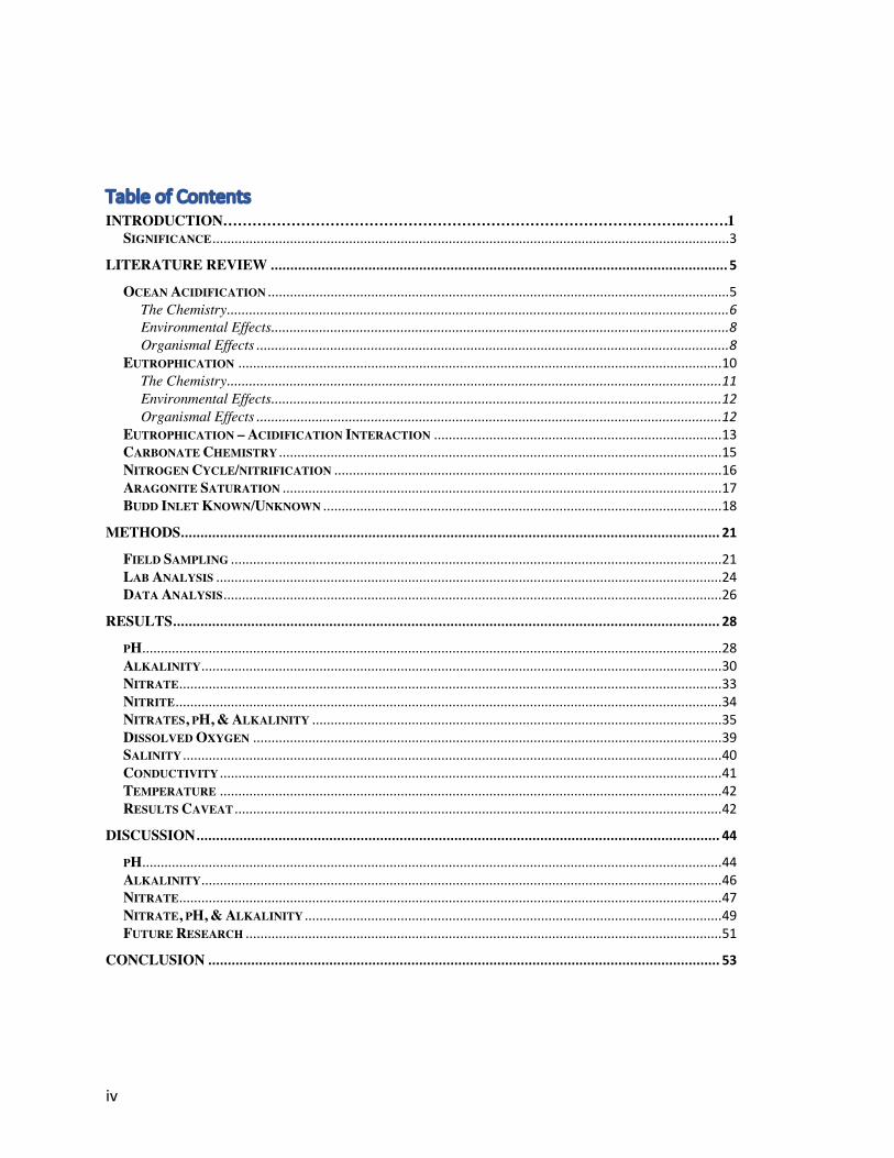
Table of Contents INTRODUCTION………………………………………………………………………………….……….1

SIGNIFICANCE ............................................................................................................................................ 3 LITERATURE REVIEW ..................................................................................................................... 5

OCEAN ACIDIFICATION ............................................................................................................................. 5 The Chemistry ........................................................................................................................................ 6 Environmental Effects ............................................................................................................................ 8 Organismal Effects ................................................................................................................................ 8

EUTROPHICATION ................................................................................................................................... 10 The Chemistry ...................................................................................................................................... 11 Environmental Effects .......................................................................................................................... 12 Organismal Effects .............................................................................................................................. 12

EUTROPHICATION – ACIDIFICATION INTERACTION .............................................................................. 13 CARBONATE CHEMISTRY ........................................................................................................................ 15 NITROGEN CYCLE/NITRIFICATION ......................................................................................................... 16 ARAGONITE SATURATION ....................................................................................................................... 17 BUDD INLET KNOWN/UNKNOWN ............................................................................................................ 18

METHODS .......................................................................................................................................... 21 FIELD SAMPLING ..................................................................................................................................... 21 LAB ANALYSIS ......................................................................................................................................... 24 DATA ANALYSIS ....................................................................................................................................... 26

RESULTS ............................................................................................................................................ 28 PH ............................................................................................................................................................. 28 ALKALINITY ............................................................................................................................................. 30 NITRATE ................................................................................................................................................... 33 NITRITE .................................................................................................................................................... 34 NITRATES, PH, & ALKALINITY ............................................................................................................... 35 DISSOLVED OXYGEN ............................................................................................................................... 39 SALINITY .................................................................................................................................................. 40 CONDUCTIVITY ........................................................................................................................................ 41 TEMPERATURE ........................................................................................................................................ 42 RESULTS CAVEAT .................................................................................................................................... 42

DISCUSSION ...................................................................................................................................... 44 PH ............................................................................................................................................................. 44 ALKALINITY ............................................................................................................................................. 46 NITRATE ................................................................................................................................................... 47 NITRATE, PH, & ALKALINITY ................................................................................................................. 49 FUTURE RESEARCH ................................................................................................................................. 51

CONCLUSION ................................................................................................................................... 53

v

List of Figures

Figure 1: Relative speciation between carbon dioxide, bicarbonate, and carbonate depending on the pH (adapted from wordpress.com). ........................................................ 7 Figure 2: Showing the connection between eutrophication (blue) and acidification (red), through biochemical pathways (black) (Zeng et al., 2014). ............................................. 15 Figure 3: Aragonite dissolution rate by species of calcifier (Ries et al., 2016). ............... 18 Figure 4: Bathymetric map of Budd Inlet sampling locations; sites are 1km apart. ......... 22 Figure 5: Budd Inlet, Olympia shoal tide chart taken from Tides.net. Sampling time started at 10:30am on 3/25/19 (A), 12:33pm on 3/27/19 (B), and 3:41pm on 3/30/19 to be during the receding tidal period. ....................................................................................... 23 Figure 6: Mean pH values at each site, showing a shallow overall increase in pH by site 30 Figure 7: Mean alkalinity results by site, showing a slight positive trend from site 1 to 5. ......................................................................................................................................... 32 Figure 8: Graph overlaying corresponding pH and nitrate values at depth -15ft. R2 shows a moderate correlation. ..................................................................................................... 32 Figure 9: Graph overlaying corresponding pH and Alkalinity values at depth -15ft. R2 shows little to no correlation. ........................................................................................... 37 Figure 10: Graph overlaying corresponding nitrate and alkalinity values at depth -15ft. R2 shows a weak correlation. ................................................................................................ 38 Figure 11: Plot is Mean nitrate concentration against mean pH at each sample location, showing a rough inverse relationship between the two. ................................................... 39 Figure 12: Comparing pH variability between month long open ocean (top) vs estuarine (bottom) measurements (Branch et al., 2013). ................................................................. 45 Figure 13: Graph showing squared pH value quantiles, showing a significant difference between sites 1 and 5, but with large, unequal variance. .................................................. 45 Figure 14: Alkalinity quantiles for each site, showing no statistical difference between sites, with an equal variance. ............................................................................................ 47 Figure 15: Nitrate quantiles for each site, showing significant difference between sites 1 and 3, and between sites 1 and 5, but with unequal variances. ......................................... 48

vi

Acknowledgements I would like to thank some influential people throughout my thesis, who

supported and enriched academic experience. First and foremost, thank you to my thesis reader Kathleen Saul for believing in me, and providing me helpful feedback and insight at every step in this process. Thank you to the Science Support Center Staff for providing access to the lab equipment and spaces, as well as getting me trained to use the Evergreen boat to perform my sampling. Thank you to all my classmates for spurring me on. I especially want to thank Hillary Foster, Bethany Shepler, and Jacob Meyers for joining me out on the boat and assisting with my sampling process, as well as helping me prepare for my thesis presentation. I also want to thank Hillary for showing me how to make maps on ArcGIS online. Lastly, thank you to my family who have supported me through my entire academic and professional ambitions.

1

Introduction

Ocean acidification (OA) is one of many large climate change consequences that have

arisen from anthropogenic carbon emissions. OA occurs when oceans absorb the carbon

dioxide (CO2) from the atmosphere, reacting with the water molecules to create hydrogen

ions, which are directly responsible for acidification. Acidification impedes sea life

functionality and survivability because organisms have adapted to a certain pH range, and

the addition of new hydrogen ions to the system changes that pH. In addition, the

hydrogen ions react with carbonate ions that organisms would normally absorb to form

shells. Those organisms cannot grow shells effectively.

Researchers have conducted many OA experiments in the open ocean, but

investigating the acidification affecting coastal and estuary systems is more difficult due

to the many extra variables that could affect the carbonate chemistry, including

freshwater input, tidal variance, and even eutrophication. This thesis will contribute to

that literature on coastal and estuary systems by examining the interaction between

eutrophication and OA, with the intent of improving upon the water quality knowledge of

Olympia, WA’s Budd Inlet.

Eutrophication results from the overabundance of nutrients in the water, 66% of

which is dissolved inorganic nitrogen, which leads to hypoxic conditions that kill off

organisms in a localized ecosystem (McCarthy et al., 2017). These nutrients largely

originate from agricultural fertilizer runoff flushing down our riverine systems. This in

turn leads to an increase in the biodegradation of those phytoplankton by microbes.

Microbes consume these algae in conjunction with a process of bacterial respiration,

which uses up dissolved oxygen (DO) and organic carbon to produce new CO2. This has

2

the net effect of increased CO2 content within the water, which then worsens the local

ocean acidification. Although the cycle described is a natural process, eutrophic

conditions exacerbate the cycle and can have a considerable influence on pH levels. OA

and eutrophication can have synergistic effects that worsen ecosystem health more than

previously thought (Freely et al., 2010). This thesis project seeks to understand the

influence of nutrients and the water’s ability to withstand these synergistic forces. The

outcome of the project will have implications for the shellfish industry, whose products

are directly affected by acidification. Coastal communities are also important as nearly

40% of the world’s populations live within 100km of coastlines, of which increasing

nutrient loads are generating from (Wallace et al., 2014).

A few marine stations/buoys within the Puget Sound basin monitor the pH, alkalinity,

and/or nutrients, which are at the heart of this thesis analysis. The alkalinity demonstrates

the buffering capacity – the water’s natural capability to neutralize its acidic components.

Alkalinity data will be compared to the pH, and nitrate + nitrite data, used here as a

primary indicator for eutrophic conditions (Garcia-Martin et all., 2017).

The research question developed into two parts. First, “Is there a significant

difference in Alkalinity, pH, and nitrate+nitrite concentrations individually between each

sample site in Budd Inlet?” Second, “Is there a correlation between the alkalinity, pH,

and nitrate+nitrite concentrations in Budd Inlet?” Four hypotheses manifested from these

questions. First, there will be a significant difference for pH and nitrate+nitrite between

each site, however there should not a be a significant difference for alkalinity. Second,

that there will be an inverse correlation between the pH and nutrient concentration. Third,

there will be a positive correlation between the alkalinity and nitrate. Fourth, there will be

3

a positive correlation between the pH and alkalinity. Alternatively, the null hypotheses

for each of these would be that there is no significant difference between sites, and there

are no correlations/variables are independent of one another.

The framework I am using to approach my research question centers around

pollution, specifically when it comes to Capitol Lake influences. The lake contributes a

significant proportion of nitrogen and low dissolved oxygen into Budd Inlet. This project

has an underlying assumption that dense urban populations, like Olympia, produce

significant amounts of pollution entering into the local water system, having a significant

influence on Budd Inlet acidification (McClelland et al., 1997; Roberts et al., 2015).

Significance

The purpose of this thesis project ultimately is to shed light on the influence that

coastal communities contribute to acidification separate from carbon emissions. Human

induced eutrophication is exacerbating acidification in coastal and estuary ecosystems,

more so than is recognized since most acidification research is not being characterized in

these terrestrial-marine boundaries in part due to the large number of variables impacting

coastlines (Reum et al., 2014). Estuary habitat, like the southern Puget Sound, have more

concern for eutrophic conditions due to the lack of flushing out of water this far inland

from the sea. The water here in Budd Inlet has a longer residence time, meaning the water

is more stagnant, in turn facilitating preferable algal habitat (Roberts et al., 2015).

Increases in nutrient loads have made the inlet’s water quality an area of concern in terms

of eutrophication and hypoxia for the state. Due to concern around eutrophication, this

project aimed to better understand the its influence these nutrient inputs have on the

4

acidification of the region. Acidification is already of great concern along coastlines

because low pH freshwater mixes with seawater, so any human action that worsens this

delicate pH balance should send a red flag to communities whom will feel its effect first

hand. This is why gathering data on nitrogen, a primary driver of eutrophication, was

necessary for this project. This is one of the three most important variables needed to

comprehend the impact humans have on OA. This project also sought to get an idea of

Budd Inlet’s current capability to buffer against such impacts to acidification. To do that,

alkalinity measurements needed to be made to understand the water’s natural buffering

capacity. This capacity presents essentially a threshold for which the water is able to

combat human influences to its pH balance. Knowing the alkalinity helps us learn how

much the ecosystem can sustainably endure before long term damage will be done, or

inversely till humans need to step in and help maintain the buffering capacity. The final

primary variable was pH because of how integral it is to OA itself. This variable is

especially crucial for marine organisms all of which are adapted for specific pH range.

pH measurements were necessary to observe the relationship to nitrogen loading. This

relationship makes up the backbone of this thesis. The goal of this project is neither to

report exact proportions of influence on this region’s OA, nor to quantify causal

relationships between each of the variables. The end goal is to simply point out that these

variables are highly relevant for this research topic, they are related to one another, and

they garner greater attention.

5

Literature Review

Ocean Acidification

Ocean acidification (OA) is concerning phenomena that occurs on a global scale due

to the ocean’s natural propensity of being a significant carbon sink for atmospheric

carbon dioxide (CO2), absorbing 28% of anthropogenic carbon emissions in the last 200

years (Wang et al., 2014). A carbon sink is almost literal in meaning. The world’s oceans

naturally absorb CO2 when in equilibrium, getting shunted down into the water and

reacting with the water molecules. Even though this is natural, the balance of absorption

is being disrupted by the sheer volume of carbon being emitted by industrial processes.

Oceans are being forced to absorb more carbon than they can manage without severe side

effects.

This is due to the Earth’s natural carbon cycle, in which, oceans are a net carbon sink.

Oceans normally exchange gases, including carbon, back and forth with the atmosphere,

but overall more CO2 is taken up in any given period of time. This is protecting people

from the full brunt of atmospheric carbon threats, but it will not stay like this forever. As

the oceans continue to warm, they will not be able to hold in carbon at the same rate,

eventually becoming super saturated leading to the outgassing of carbon (Wang et al.,

2014). This essentially turns the oceans into a net carbon source that will release carbon

back into the atmosphere. This is not predicted to happen anytime soon, but the rate at

which carbon is absorbed will decrease significantly by the year 2100 (Wang et al.,

2014).

Currently the world’s oceans have dropped from about 8.2 to 8.1 pH, however this is

a large percentage change in pH, about 30% (Bianucci et al., 2018; NOAA PMEL). By

6

the year 2100 the pH is expected to drop to 7.8, which is a 151% alteration from 8.2

(NOAA PMEL; Reum et al., 2014). The problem with coastlines and estuaries is they

usually experience more acidified conditions of less than a 7.7pH (Wallace et al., 2014).

On top of this, oceans are not expected to be able to absorb as much carbon by the year

2100 compared to now, reducing the mitigating effect they have on atmospheric carbon

(Wang et al., 2014). This is highly problematic since most of the marine life on earth live

near shallow coastal regions and are sensitive to changes made in the pH they are adapted

to (Fondriest, 2014). On top of that, even though many OA experiments have been done

on the open ocean, few have been performed for the effects on coastal and estuary

systems, emphasizing a need for this research.

The Chemistry

Acidification is a straightforward process with a few steps. First, once the CO2 is

absorbed into the ocean, it will dissolve into an aqueous solution where it can then

chemically react with the water molecules. Aqueous means that the gaseous CO2 is now

dissolved into the liquid, as opposed to being a stand-alone bubble within the water. This

is when the aqueous CO2 is able to react with H2O as seen in the acidification equation

below. This will produce a new molecule known as carbonic acid (H2CO3), which is a

normally a short-lived molecule as only one percent of carbon is in this form. It then

dissociates into bicarbonate (HCO3-) and a one hydrogen ion, the ion directly responsible

for acidification. The bicarbonate speciation holds the largest proportion of initial carbon

at around 90% (Branch et al., 2013). The bicarbonate will further dissociate into a

carbonate ion (CO32-) and another hydrogen ion, with carbonate comprising roughly nine

7

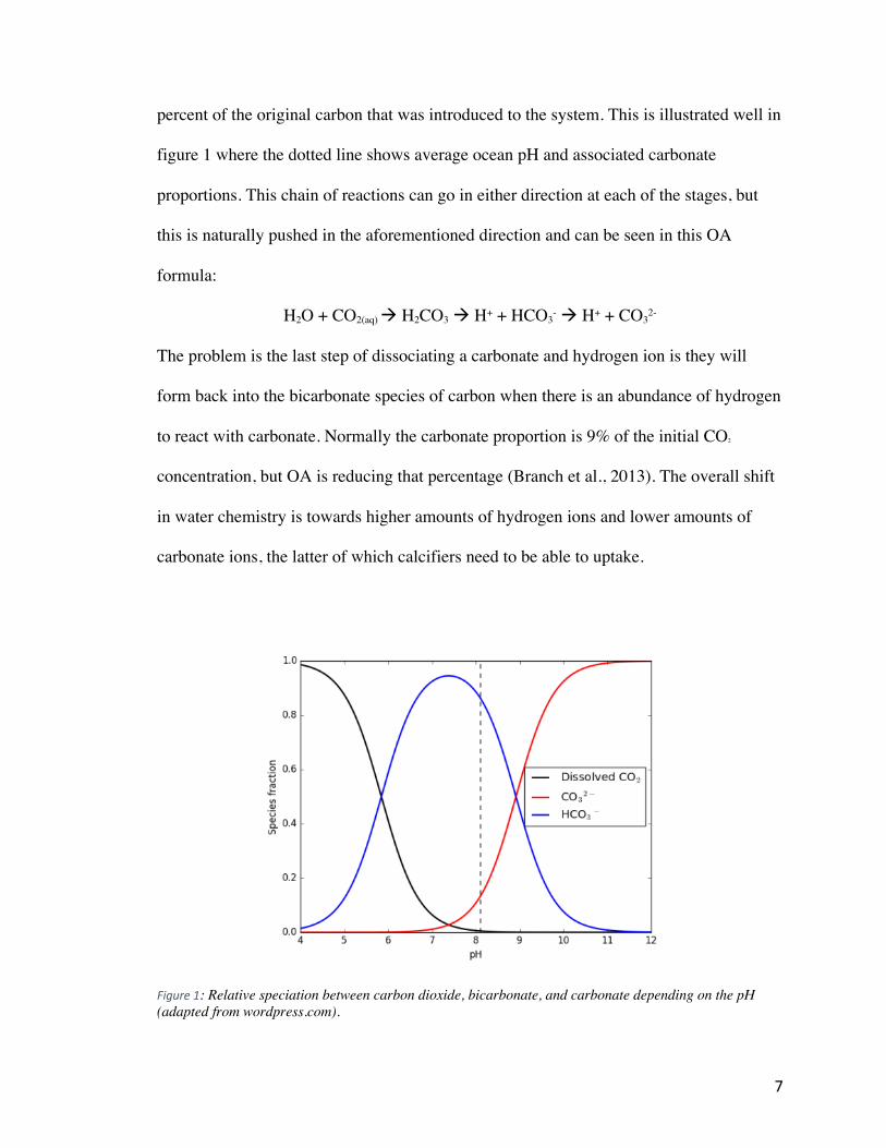
percent of the original carbon that was introduced to the system. This is illustrated well in

figure 1 where the dotted line shows average ocean pH and associated carbonate

proportions. This chain of reactions can go in either direction at each of the stages, but

this is naturally pushed in the aforementioned direction and can be seen in this OA

formula:

H2O + CO2(aq) à H2CO3 à H+ + HCO3- à H+ + CO3

2-

The problem is the last step of dissociating a carbonate and hydrogen ion is they will

form back into the bicarbonate species of carbon when there is an abundance of hydrogen

to react with carbonate. Normally the carbonate proportion is 9% of the initial CO2

concentration, but OA is reducing that percentage (Branch et al., 2013). The overall shift

in water chemistry is towards higher amounts of hydrogen ions and lower amounts of

carbonate ions, the latter of which calcifiers need to be able to uptake.

Figure 1: Relative speciation between carbon dioxide, bicarbonate, and carbonate depending on the pH (adapted from wordpress.com).

8

Environmental Effects

Ocean acidification by definition has elevated levels of dissolved carbon dioxide

within the water. pCO2 (CO2 partial pressure) has risen as a result of carbon emissions

along and reduced carbonate species minerals (Reum et al., 2014). Partial pressure is a

measure of the total volume that would be occupied by only the dissolved CO2 in a given

area as opposed to a general measurement of the total volume of all dissolved gases

within that same given area. pCO2 is an indirect measure used to determine pH, and it is

also useful in OA research for its direct relation to anthropogenic emissions as well as its

direct relation to aragonite concentrations (Reum et al., 2014).

Acidification itself exacerbates the overall pollution of the water. This feedback loop

happens because lower pH water is absent of anions like carbonate and hydroxide (OH-)

that would normally bind with inorganic heavy metals, and thereby buffering against OA

(Zeng et al., 2014). There are not many toxic metals already in the water, especially since

most are locked up in organic molecules, however, even small increases may result in

higher water toxicity that animals may have a hard time coping with (Zeng et al., 2014).

Organismal Effects

OA causes many problems for sea life because the hydrogen ions react with carbonate

to form bicarbonate when calcifying animals normally need carbonate to react with

calcium ions to build calcium-carbonate shells, which renders the carbonate useless for

those animals. These shell building and calcifying organisms are the species most

affected by OA for this reason. Mollusks and crustaceans alike are of greatest concern

because of their almost direct reliance on a pH balance and how much people rely on

9

them heavily as a food and economic source. Not only does lowering the pH interfere

with their biological ability to form hard shells by making them more brittle and soft, but

it can also impede metabolism function, growth, overall survivability especially at early

life stages (Carter et al., 2013; Long et al., 2013; Swiney et al., 2017).

Calcification is a process by which creatures like crustaceans, mollusks, and coral

take in calcium-carbonate to form their shell. OA has the effect of making it more

difficult for crustaceans to physiochemically uptake calcium and carbonate ions in order

to form a calcium-carbonate shell, although not to as great a degree as seen in mollusks

(Branch et al., 2013). Early life stages are most vulnerable to external pressures including

low pH values due to their sensitivity to water quality changes that they are specifically

adapted for. Metabolism is also negatively affected by lower pH values, with the largest

responses seen by embryos in most species. This is possibly due to the energy cost from

longer development times before hatching. Calcifying organisms have a specific pH

range for successful fertilization and falling outside of that range will reduce that number

(Byrne, 2011). Researchers have also found evidence for “hypercapnia-induced

metabolic depression” in embryos, which impairs their capability for internal acid-base

regulation and suppresses their metabolic efficiency (Byrne, 2011; Carter et al., 2013).

Hypercapnia is a condition in which there is too large a buildup in CO2 within the blood

stream. This lowering of the metabolic rate is initially good for the crab in the short term,

but a continuous lowered metabolic rate will reduce any organism’s overall fitness and

general metabolic maintenance (Carter et al., 2013).

Less available carbonate causes calcifying organisms will create a thinner and softer

shells, making them susceptible to predation (NOAA, 2016). Calcifiers were found to

10

have negatively correlated pH sensitivity to the usage of aragonite calcite types at the

family, order, and class level (Busch & McElhany, 2017). Tolerance to acidification is

partly dependent on degree of control over the process of calcification (Kroeker et al.,

2013).

Researchers also found that acidified water decreased the molting success rate in

crustaceans (Long et al., 2013). There larger implications for the stresses that crustaceans

face during molting sessions since crabs molt multiple times in their lifecycle, more when

they are young and less as crustaceans mature to adulthood. Calcifiers are

disproportionately weakened in acidic water than they otherwise would be (NOAA

Fisheries, 2016).

Eutrophication

One large environmental issue present in the south Puget Sound is an abundance of

nutrient inputs causing a eutrophic environment. Eutrophic waters tend to cause algal

blooms since the limiting factor of nitrogen is now in a surplus, thus increasing their

primary productivity (Wallace et al., 2014). Eutrophication is happening for three main

reasons in the south Puget Sound. First, the seasonal conditions are conducive to algal

blooms such as in the late summer/early fall. Second, there is poor cycling and flushing

out of the water in a certain region due to local geography. Third is the high level of

pollution entering the water body (Wallace et al., 2014). The latter reason is the largest

contributor to most eutrophic situations that occur. Large amounts of nutrients enter the

water system from rivers and from overland runoff. Rivers tend to contain lots of excess

nutrients from agricultural fertilizer, while urbanized coastal regions tend to have a lot of

11

storm water runoff that carries nutrients and pollutants over the impervious surfaces in a

city. Eutrophication is a natural process however humans are making conditions more

amenable to algal blooms.

The Chemistry

There are three parts in understanding eutrophication; in chronological order they are

the nutrient load, algae primary productivity, then algal and microbial respiration. These

three factors comprise the full eutrophication process. Eutrophication literally is the

overabundance of nutrients, mainly nitrogen and phosphorous, that leads to an

overgrowth of plant life. Whether the nutrients come from agricultural inputs into rivers,

or storm water runoff through the city, they are greatly reducing the local water quality at

the point of entry. Once the nutrients enter a water body, they begin to stimulate the

primary production of plant life namely phytoplankton. Nitrogen is a limiting nutrient, so

increasing the available concentration will allow phytoplankton to balloon in population

(Garcia-Martin et al., 2017). Phytoplankton utilize photosynthesis to create their own

energy by absorbing sunlight and CO2 during the day. This process produces oxygen and

glucose. At night they go through a process of respiration where they go through the

reverse of the process. During respiration, the plankton uptake oxygen and produce CO2

(Wallace et al., 2014). Altogether the process of photosynthesis and respiration is known

as the biological pump (Wang et al., 2014). Photosynthesis would normally be helpful in

controlling the amount of dissolved carbon, however the rates of respiration are greater,

leading to a net increase in the dissolved carbon (Garcia-Martin et al., 2017).

12

Environmental Effects

Hypoxia is one of primary issues that occurs during an algae bloom in a eutrophic

environment. Hypoxia is an extremely low dissolved oxygen (DO) condition with a

standard threshold of about 2mg/L that prevents many organisms living in the water from

thriving. (Freely et al., 2010). This occurs because overactive microbial populations

consume oxygen in order to break down the algal blooms that resulted from excessive

nutrient inputs faster than the oxygen can be replenished (Wallace et al., 2014).

Another result from the introduction of high nutrient loads and pollution is that

organisms have a weakened capacity to photosynthesize in the first place (Zeng et al.,

2015). With less total photosynthesis occurring, more CO2 is free to react with water and

further acidify.

Organismal Effects

The primary organisms that benefit from eutrophic conditions are

algae/phytoplankton. They consume the excess nutrients and carbon dioxide to grow and

reproduce. These algal blooms are problematic because they create acutely anoxic

conditions (lacking oxygen) that few marine organisms can tolerate. Most organisms

cannot survive in low oxygen waters because it prevents aerobic respiration of marine

organisms, effectively suffocating them. Hypoxia (low dissolved oxygen) will typically

kill off large numbers of fish, throwing the local ecosystem out of equilibrium.

Nitrogen and phosphorus are considered limiting nutrients in the environment

because growth can only occur as long as they are available. Nitrogen is usually more

important to plants than phosphorus because the ratio they require in their body makeup.

13

A ratio of 7.2:1 nitrogen to phosphorus tends to be the sweet spot that plants prefer

(Roberts et al., 2015). In many freshwater environments, phosphorus tends to be the

limiting nutrient, however, that is not the case in marine environments. Typically, in

marine waters like the Puget Sound, nitrogen is less prevalent, therefore making it the

limiting nutrient (Roberts et al., 2015). Excess nitrogen can be introduced through

streams and runoff along coastal and estuarine environments. In recent decades, this has

increased the amount of algal blooms around those areas (McClelland et al., 1997).

Eutrophication – Acidification Interaction

The linkage between eutrophication and OA occurs at the tail end of the

eutrophication process where microbial activity contributes to CO2 inputs. In eutrophic

conditions, there is a prolific amount of nutrients including, but not limited to nitrate,

phosphorous, and ammonia in the water as a result of runoff from agricultural practices

or general pollution from urban populations. As indicated earlier, excess nutrients

facilitate the ballooning of algae and phytoplankton growth and reproduction rates.

Microbes then consume the algae and phytoplankton as they die, in a process called

biodegradation. This process requires microbes to consume oxygen, so as more algae get

eaten, the dissolved oxygen in the water column becomes depleted. This results in

hypoxia, and is commonly defined as having equal to or less than 3mg/L of dissolved

oxygen near the floor of the water body (since that is where detritus falls to and microbes

consume the oxygen when breaking down organic material) (Wallace et al., 2014). DO

values often fall close to hypoxic levels in the Puget Sound, which averages between 9-

10.7mg/L (Freely et al., 2010).

14

Microbes increase their primary productivity and combine their consumed oxygen

with the organic matter they break down to produce new CO2, leading to a net increase in

CO2 in the system (Freely et al., 2010; Wallace et al., 2014). The CO2 will react with the

water molecules in the same way as CO2 coming from the atmosphere, acidifying much

more than compared to non-eutrophic water quality. The amount of microbe productivity

is primarily determined by how much dissolved organic matter is present to consume to

create energy (Garcia-Martin et al., 2016). Once they remineralize this organic material

with DO, they respirate out CO2, leading to the net increase in CO2, despite algae taking

CO2 out of the water to photosynthesize (Freely et al., 2010). This entire process is

illustrated in Figure 2 where eutrophication is introduced into the ecosystem in blue, on

the left and goes through biochemical pathways, in black, to become converted into

dissolved CO2 that goes through the acidification process, shown in red. Since the level of

algae and microbe productivity, and the observed acidification is much greater along

coastal and estuary ecosystems than one would calculate solely based on carbon

emissions. Scientists theorize that high nutrient loads are causing the increased intensity

of acidification observed in these regions (Garcia-martin et al., 2016; Wallace et al.,

2014).

15

Figure 2: Showing the connection between eutrophication (blue) and acidification (red), through biochemical pathways (black) (Zeng et al., 2014).

Carbonate Chemistry

Carbonate system dynamics are integral to this project. Carbonate chemistry involves

the relative proportions and interactions between different carbonate molecules and

variables that influence these proportions and interactions. Carbonate (CO3) manifests in

different forms that influence water quality dynamics. In one example, calcium-carbonate

is crucial for calcifying organisms to grow their shells. The availability of free

carbonate becomes an issue when oceans uptake too much CO2 with the end result being

a lower concentration of available carbonate that can combine with calcium for these

marine organisms (Branch et al., 2013).

There are three main forms of carbonate that occur during OA, as explained in the

“OA chemistry” section. In short, carbonic acid, bicarbonate, and carbonate are formed

through a series of reactions between CO2 and water. Other important variables

16

associated with carbonate chemistry include dissolved inorganic carbon (DIC) or pCO2,

pH, DO, and aragonite. The proportions of the three forms of carbonate depend on these

other variables, but the key one is the pH. As seen in figure 1, a higher pH is needed to

facilitate higher concentrations of carbonate. Oceans have an average pH of 8.1 meaning

that available carbonate will likely always be a limiting factor. As pH levels decrease to

the mid-range, the available carbonate drops even further, where high bicarbonate

(HCO3) proportions are favored. Decrease pH even further facilitates high CO2

proportions with carbonate practically being snuffed out (also shown in Figure 1).

Nitrogen Cycle/nitrification

The nitrogen cycle explains how nutrients impact water quality. Nitrogen can come in

organic, inorganic, dissolved, and particulate forms, but the form to pay most attention to

in the context of OA would be dissolved inorganic nitrogen (DIN). DIN commonly

denotes the nitrate concentration but authors and researchers may also include nitrite and

ammonia in their calculation of nitrogen, depending on the experimental focus.

Following that lead, both nitrate and nitrite were chosen in this project to represent

nitrogen.

DIN is introduced into the ecosystem through agricultural practices, wastewater

effluent, urban communities, runoff, etc. DIN goes thorough process of nitrification:

different forms of nitrogen are oxidized, converting it from ammonia to nitrite, and

oxidized again from nitrite into nitrate (Pelletier et al., 2017).

17

Aragonite Saturation

Aragonite, as a preferential form of carbonate, is one of the most important mineral

resources for calcifying organisms and is highly dependent on the water’s pH balance.

Many calcifiers preferentially select for aragonite due to how common and soluble it is,

having a medium Mg-calcite content (Ries et al., 2016). Aragonite is the chosen

polymorph of calcite or calcium carbonate (CaCO3) used in many OA studies because it is

so integral to carbonate chemistry. This mineral’s solubility is determined by its

saturation state and is directly sensitive to pH changes; a lower pH has a large reduction

effect on solubility (Long et al., 2016).

Researchers use Warg to denote the aragonite saturation state, with oversaturation

being [W>1], equilibrium saturation [W=1], and an undersaturated state being [W<1]

(Branch et al., 2012). Calcifying organisms prefer a saturation greater than one in order to

easily uptake calcite without expending a lot of energy (Branch et al., 2013).

Undersaturated aragonite will drive the reaction in the opposite direction, effectively

dissolving calcium-carbonate, which requires organisms to use much more energy to

uptake these ions (Branch et al., 2012). A low pH is associated with a low aragonite

saturation state, with undersaturated states appearing near pH of 7.5 (Long et al., 2016).

Aragonite must have a saturation state equal to or greater than one in order for it to

precipitate and be available to calcifying animals, whilst undersaturated water (<1) will

dissolve the aragonite (Reum et al., 2014). This is illustrated in Figure 3 where all

calcifying species’ shells began dissolving once the aragonite saturation state begin to

approach “one.” Maintaining a saturation state greater than one is difficult with low

alkalinity and high nutrient conditions present in Budd Inlet, as explained in the results

18

section later. these forces hamper stable aragonite levels, thus creating unfavorable

aquatic habitat for all calcifying organisms.

Figure 3: Aragonite dissolution rate by species of calcifier (Ries et al., 2016).

Budd Inlet Known/Unknown

Currently much of the South Puget Sound is an area of concern for Thurston County

and the State of Washington due to the low oxygen and high nitrogen levels. In

particular, since 2014 most of Budd Inlet has been designated for having major water

quality impairments (McCarthy et al., 2017). The largest negative influence to Budd Inlet

is Capitol Lake. Capitol Lake has had many water quality issues for decades and was

19

closed to all public usage in 2009. These negative water quality impacts consist primarily

of high nutrient and low DO concentrations (Roberts et al., 2015).

Alkalinity data for Budd Inlet is limited. However, Taylor Shellfish of Shelton, WA

takes measurements of alkalinity daily, albeit towards the northern Puget Sound.

Nonetheless water samples of Budd Inlet are anticipated to be similar to the overall

content of Puget Sound water, which is primarily seawater, with some influx of

freshwater from Capitol Lake and other smaller creeks and streams. Taylor Shellfish,

during the time of sampling, reported average alkalinity concentrations to be around 180-

200mg/L, which will be the assumed baseline measurement for Budd Inlet as well

(IPACOA, 2019).

Nitrogen values in Budd Inlet are expected to fall within 0.1 and 1mg/L when mixing

fresh and saltwater, with an average of 0.5mg/L during the time of sampling in late

March (McCarthy et al., 2017; Roberts et al., 2015). Generally, nitrate values vary with

the season, day, and depth.

Estuaries are unique ecosystems in that they are transitional zone between fresh and

salt water. These coastal zones are necessary provide brackish water for certain

organisms that are anadromous, meaning they are able to travel between fresh and

saltwater systems. Estuaries provide a special transitional habitat for that migration.

Many species are also adapted for such brackish waters, and estuaries have well suited

habitat for many different species compared to a typical coastline. pH values in the more

saline estuary portions tend to range between 8-8.6 today, while freshwater tends to have

lower pH values between 7-7.5 (EPA, 2006). Due to the conductivity and salinity values

measured in Budd Inlet being closer to average saltwater values, water samples were

20

expected to be most closely related to salt water than freshwater. pH values therefore are

anticipated to be a mixture between salt and freshwater, likely being closer to the salt

water range somewhere between 7.5 and 8.0 based off EPA ranges mentioned above.

Ocean Acidification and eutrophication are intrinsically linked at the junction where

algal blooms lead to microbes creating anoxic conditions and introduce new CO2 into an

ecosystem. Understanding the carbonate chemistry and nitrogen cycle helps to inform

how the components of OA and eutrophication propagate. Nutrient inputs are having

compounded effects on pH reductions along with greenhouse gas emissions. This is

stressing marine organisms by reducing the availability of carbonate, and creating a low

saturation state that will cause the dissolution of shelled organisms. These impacts are

happening in Budd Inlet through the influence of Capitol Lake nutrient inputs, prompting

this research.

21

Methods

Field Sampling Five points along a sampling transect were designated for sample collection with each

of the five sites set to one kilometer distances between one another starting near the point

of the peninsula towards the West Bay in the southern end of Budd Inlet. After the first

sampling location was determined, subsequent locations were measured one kilometer

north until five points were logged. The transect was chosen to be as close to the center of

the inlet as possible while having a minimum 20 foot depth.

The GPS coordinates for each sampling site were saved into Garmin Echomap DV

GPS so that each site could be revisited accurately for multiple sampling sessions shown

in figure 4. At each site 60mL of unperturbed water was gathered using a Wildco 1100-

1900 series vertical Van Dorn water sampler, captured at a 15 foot depth to perform an

alkalinity and nutrient analysis. The 15 feet depth was chosen in order to be consistent

with retail shellfish grower and seller Taylor Shellfish’s 15 feet measurement depths at

Dabob Bay in Jefferson County. Taylor Shellfish collects and publishes live alkalinity

and pH data, two major variables needed for my experimental analysis. A 15 foot depth is

also beneficial because it lies below the surface air-water interactions that could skew

data gathered (Moore et al., 2014).

22

Figure 4: Bathymetric map of Budd Inlet sampling locations; sites are 1km apart.

In addition to the water samples, water column profile measurements were also

collected at each site using a 2030 YSI Pro from 0-20 feet at five foot increments, for a

total of five depths. This was intended to provide a more holistic snapshot of the water at

each sampling site at that given time, although the 15 foot measurements are the most

important to compare to gathered water samples. The variables acquired consisted of

dissolved oxygen (DO), salinity, temperature, and conductivity. These measurements are

also collected by Taylor Shellfish the Seattle Aquarium, King County’s Point Williams

buoy, and many others. Data collection was repeated at each site three times: on 3/25/19,

23

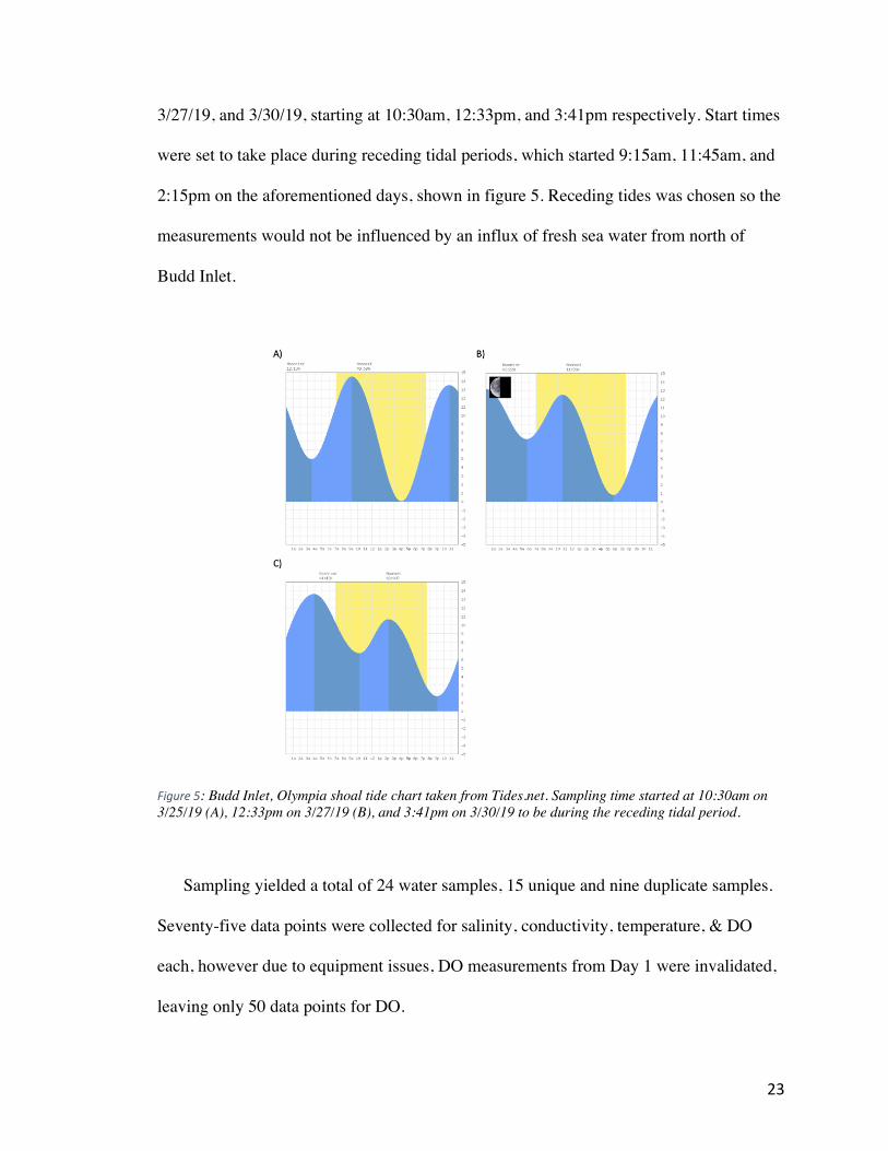
3/27/19, and 3/30/19, starting at 10:30am, 12:33pm, and 3:41pm respectively. Start times

were set to take place during receding tidal periods, which started 9:15am, 11:45am, and

2:15pm on the aforementioned days, shown in figure 5. Receding tides was chosen so the

measurements would not be influenced by an influx of fresh sea water from north of

Budd Inlet.

Figure 5: Budd Inlet, Olympia shoal tide chart taken from Tides.net. Sampling time started at 10:30am on 3/25/19 (A), 12:33pm on 3/27/19 (B), and 3:41pm on 3/30/19 to be during the receding tidal period.

Sampling yielded a total of 24 water samples, 15 unique and nine duplicate samples.

Seventy-five data points were collected for salinity, conductivity, temperature, & DO

each, however due to equipment issues, DO measurements from Day 1 were invalidated,

leaving only 50 data points for DO.

24

All water samples were filtered through 0.45um cellulose filter syringe on site in

order to remove larger particulates, such as chlorophyll, then stored in an ice cooler until

they could later be transferred to a refrigerator to preserve them.

Lab Analysis Two separate lab experiments were performed to determine the nutrient content and

total alkalinity (TA) of the water samples. In order to figure out the nutrient content, the

nitrate+nitrite concentration was specifically designated and is the most widely used

nutrient measurement utilized in eutrophication research. These nitrogen species are

associated with primary productivity and are a good proxy for eutrophic conditions

(Garcia-Martin et al., 2016; Xu et al., 2014). In addition, nitrate (NO3) is the only

continuous nutrient measurement being taken in the Puget Sound by King County’s Point

Williams buoy. Due to lab complications, the nitrite concentrations were not able to be

measured, which will be elaborated in the results section. Other chemicals such as

phosphorous or ammonia also add to the total contribution of nutrient loading in a given

ecosystem, but the most commonly reported value is nitrate concentration. This, along

with general time and resource limitations led to a focus on nitrate in this research. pH

data were also taken independently as well as during alkalinity tests.

The nitrate analysis was performed using Schnetger & Lehners’ 2014 vanadium

chloride reduction procedure. This procedure requires a stock solution of sodium nitrate

(NaNO3) and sodium nitrite (NaNO2) being created. A 40mM stock solution of NaNO2

and NaNO3 was made. Both stock solutions were then diluted into nine molarities in order

25

to create a calibration curve. These molarities were 2uM, 4uM, 10uM, 20uM, 30uM,

40uM, 50uM, 60uM, and 70uM. This range was designed to encapsulate the full breadth

of nitrate and nitrite concentrations that may be present in Budd Inlet based on the

average nitrate values measured in real time by the Point Williams buoy in South Seattle

along with other published materials. The nine points also increased the calibration

curve’s accuracy. Four different primary reagents were then created for the reduction and

isolation of nitrates, labeled as reagents A through D. Additional reagents, labeled E and

F, were then created for the nitrate and nitrite extraction according to the ratios laid out in

Schnetger & Lehners’ paper. Reagent E combined the first, second, and third reagents.

The sixth and final reagent combined the first and second reagents.

The next step involved pipetting aliquots of these reagents and samples into the 96

well plate to be analyzed on a UV/vis Spectramax Plus spectrophotometer. A new

calibration curve was created for each batch of samples being tested. Two batches of

every sample were created, with each batch being run twice on the spectrophotometer to

increase the sample size. An R2 significance value of 99.5% or higher was required to

validate accurate measurements.

The total alkalinity (TA) experiment was done to determine the water’s buffering

capacity – the water’s natural capability to neutralize its acidic components. The main

neutralizing components in this test was the bicarbonate concentration which is

dependent on its pH. The TA was assessed using the USGS’ 2012 standard water quality

and field sampling titration procedures along with Dr. Erin Martin’s titration procedures,

which were adapted from the USGS methods (Martin, E., 2019).

26

The alkalinity test required a Sulfuric acid (H2SO4) titrant solution to be created; a

final concentration of 0.025M or 0.05N was created. The pH probe and meter was

calibrated prior to each sample titration. Water samples were set out at room temperature

until their temperature stabilized in order to perform the titration consistently, although

this was a limitation, not being able to perform titrations at their original temperature.

Each sample was titrated to a pH below 4.0 utilizing a Gilmont micrometer buret.

Samples were titrated in larger increments to start, then in smaller increments until the

desired pH was reached. The pH and temperature was recorded after each allotted acid

titrant.

Data Analysis An Analysis of Variance (ANOVA) statistical test was performed on nitrate,

alkalinity, and pH measurements using the JMP 2014 program provided by Evergreen

State College. ANOVA is applicable here because there were five distinct groups that

needed to be tested against each other (i.e. each sampling location). ANOVA was also

useful since it is very robust against deviations around the mean. This was a concern here

due to smaller sample sizes present in the experiments and measurements, as well as the

data not all being normally distributed, having high variability. ANOVA allows for a

determination of statistically significant differences between each site from another. This

test was able to point out which of the five site locations, if any, were significantly

different. ANOVA has a primary assumption that the means have equal variance. The

27

null hypothesis for an ANOVA test for any of the variables was that the mean between all

five sites were the same (H0= u1 = u2 = u3 = u4 = u5).

The alternative hypothesis for each test was that at least one of the sample locations

was different from the others, however an additional Tukey-Kramer HSD test is required

to determine which mean is different from the others. pH and nitrate data did not have a

normal distribution and were transformed by taking the square and log respectively,

which were the most normally distributed histograms chosen for running the ANOVA.

Three major variables were plotted against each in a normal scatter plot to see if there

was a correlation between the variables. This included graphing the alkalinity values

versus the pH, alkalinity versus nitrates, and pH versus nitrates. Once a graphed, a

trendline and R2 value were generated to see if there is a positive or negative trend and the

level of correlation between variables. The correlation explained what percent of a

change in Y can be explained by a change in X.

28

Results The data explained below encompasses lab analysis results for pH, alkalinity, and

nitrate concentrations, as well as field measurements for DO, salinity, conductivity, and

temperature. pH, alkalinity, and nitrate constitute the most important reported results and

have their own dedicated sections in the literature review explaining the historical and

current expected figures for these variables.

There are two research questions that require pH, alkalinity, and nitrate in order to

answer. First, “Is there a significant difference in pH, alkalinity, and nitrate between each

of the five sampling sites?” This question based on the knowledge that high nutrient loads

are coming primarily from Capitol Lake as explained in the literature review.

Concentrations are more influenced closer to southern most sampling site compared to

the northernmost site. The second research question being answered here is “Is there a

correlation between pH, alkalinity, and nitrate?” This research does not aim to determine

causal relationships but seeks to determine if there is a trend of association between these

variables.

Nitrite concentrations will not be used to answer the research question, as explained

later in the results section. The end of the results section includes a paragraph speaking to

the limitations of these results.

pH The observed pH values came out to be close to expected values for a mixture of

fresh and saltwater. These measurements confirm that estuaries, like Budd Inlet, have

lower pH levels than the open ocean. Ocean acidification has caused the pH of the open

29

ocean to drop from 8.2 to 8.1. This is in contrast to the average pH value of 7.86 found in

this project. If a reduction in pH from 8.2 to 8.1 amounts to about a 30% lower pH, then

the difference between 8.2 to 7.86 amounts to almost a 125% lower pH than the open

ocean (NOAA PMEL, 2018). This is a much lower pH, however these results are not too

surprising because mixed freshwater and saltwater could range from 7.5-8 (EPA, 2006).

This average pH value of 7.86 suggests the water more closely resembles saltwater,

which is consistent with other variables measured in the field.

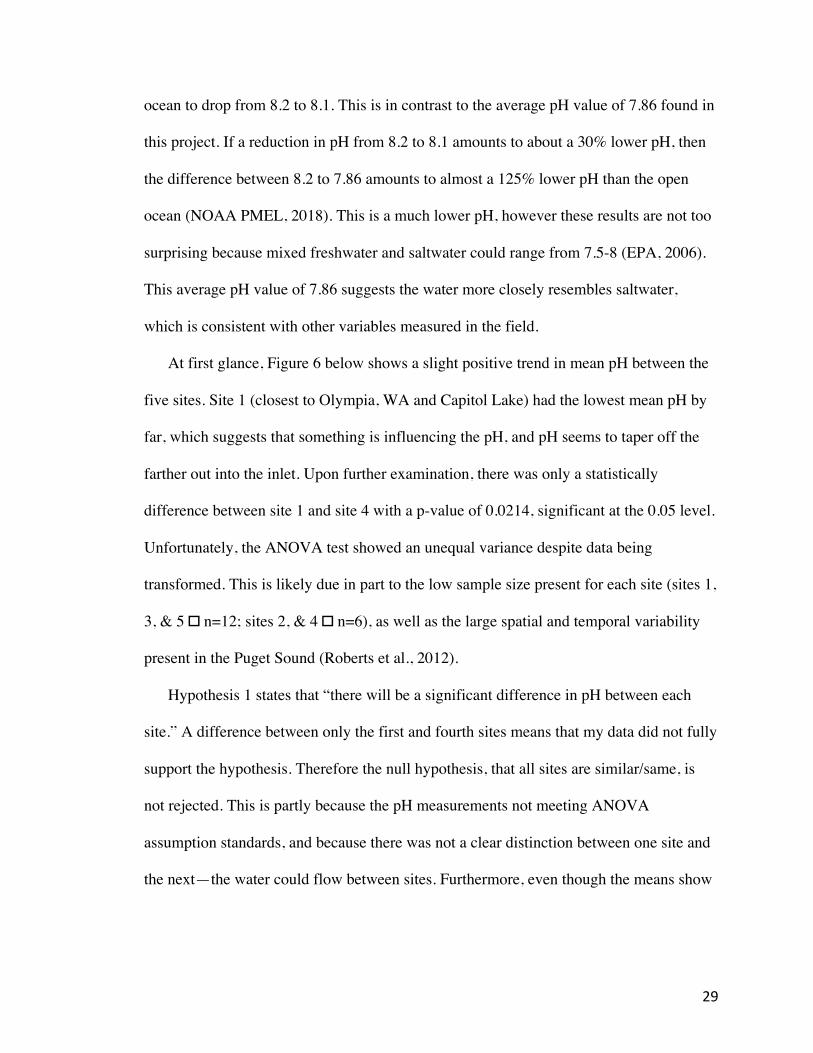
At first glance, Figure 6 below shows a slight positive trend in mean pH between the

five sites. Site 1 (closest to Olympia, WA and Capitol Lake) had the lowest mean pH by

far, which suggests that something is influencing the pH, and pH seems to taper off the

farther out into the inlet. Upon further examination, there was only a statistically

difference between site 1 and site 4 with a p-value of 0.0214, significant at the 0.05 level.

Unfortunately, the ANOVA test showed an unequal variance despite data being

transformed. This is likely due in part to the low sample size present for each site (sites 1,

3, & 5 � n=12; sites 2, & 4 � n=6), as well as the large spatial and temporal variability

present in the Puget Sound (Roberts et al., 2012).

Hypothesis 1 states that “there will be a significant difference in pH between each

site.” A difference between only the first and fourth sites means that my data did not fully

support the hypothesis. Therefore the null hypothesis, that all sites are similar/same, is

not rejected. This is partly because the pH measurements not meeting ANOVA

assumption standards, and because there was not a clear distinction between one site and

the next—the water could flow between sites. Furthermore, even though the means show

30

a roughly linear gradient going from the first to the last site, the variation within each site

was too great to say the sites were actually different from one another.

The research results cannot determine the relative proportion of impact to pH from

greenhouse gasses or nutrient loading. It will, however, provide insight into the observed

pH level drops.

Figure 6: Mean pH values at each site, showing a shallow overall increase in pH by site.

Alkalinity Titration data was calculated with a USGS alkalinity calculator, along with alkalinity

hand calculations made from the same set of titration data to increase the total sample

size. Data was then entered into ANOVA to be analyzed for site differences. At face

value, the mean alkalinity values in Figure 7 look low at the first site and increase as one

goes further out into the inlet. This makes some sense since freshwater influx would

contain lower alkalinity levels and contribute significantly to the decrease in overall

alkalinity (Fry et al., 2015). The second hypothesis for alkalinity states that “there will be

R² = 0.6185

7.607.657.707.757.807.857.907.958.00

1 2 3 4 5

pH

site

mean pH

31

a positive relationship in alkalinity by distance going north up Budd Inlet,” with site 1

having the lowest value and site 5 having the highest value. The null is that there is no

difference between any of the sites. It is important to say that the expectation is for the

null hypothesis to be true because there should not be significant influences to alkalinity

coming from southern end of Budd Inlet.

ANOVA results showed no statistical difference between the alkalinity of the five

sites. These results met the assumption of equal variance. This means the null hypothesis

cannot be rejected. Despite not having any statistical difference, similar values make the

most sense because the biggest influences on alkalinity are the mixing of fresh and

saltwater, and alkalinity tends to have more stable variation throughout the year

(Fassbender et al., 2018). Small changes between each kilometer in distance away from

Olympia should not result in values that are distinguishable from each other.

Additionally, there should be no difference between sites for alkalinity since alkalinity

showed little to no correlation to either the highly variable pH or nitrate levels. The

alkalinity should remain relatively homogenously mixed within the water column

because alkalinity is less variable and more stable over time (Bianucci et al., 2018;

Fassbender et al., 2018). Alkalinity is not significantly influenced by changing pH or

nitrate levels, therefore expected values should not change regardless of pH and nitrate

influences.

32

Figure 7: Mean alkalinity results by site, showing a slight positive trend from site 1 to 5.

Having the same alkalinity, but with differing nitrate values could lead to different pH

values between sites. This would mean the nitrates would correlate to the pH, as is shown

to be the case in Figure 8. Assuming the buffering capacity (as reflected in alkalinity) of

Budd Inlet is constant, the increased concentration in nutrients entering into the inlet will

reduce the pH. It is important to note that the buffering capacity is not changing here;

there is a reduced capability of the water to maintain a stable pH.

Figure 8: Graph overlaying corresponding pH and nitrate values at depth -15ft. R2 shows a moderate correlation.

R² = 0.1714

100.00

101.00

102.00

103.00

104.00

105.00

1 2 3 4 5

alka

linity

(mg/

L)

site

mean alk

R² = 0.2754

7.57.67.77.87.9

88.1

3.00 4.00 5.00 6.00 7.00 8.00 9.00 10.00

pH

Nitrate (uM)

pH vs NO3

33

Alkalinity values averaged 101.87mg/L or (1018umol/kg) across all sites. These

measurements are consistent with average estuarine alkalinity values, which average

116mg/L (EPA, 2006). The main factor contributing to this difference in buffering

capacity is the influence of freshwater flowing in from the Deschutes river, as well as

other freshwater sources (Thurston County Water Resources Report, 2018). Freshwater

alkalinity values fall between 30-90mg/L, and this combines with the fact that the water

in the lower Puget Sound does not get flushed out easily, having a longer residence time

(EPA, 2006). The aggregate effect results in a below average buffering capacity.

Nitrate Nitrate concentrations, after being measured in the lab, were analyzed using an

ANOVA statistical test to determine if there was a significant difference between sites.

The third nitrates hypothesis states that “nitrogen concentrations would show a negative

gradient” with higher values in the southern most sampling location (Site 1) and lowest

the location furthest away (Site 5). This hypothesis is based on the idea that sources of

nitrates would originate from Capitol Lake and runoff from the ports, and dissipate/dilute

as one goes further out into the inlet due to mixing of incoming seawater containing

lower background concentrations of nitrates (Roberts et al., 2012; Roberts et al., 2015).

The null hypothesis reflects this: There is no difference between any of the sampling sites

or that all sites would have equal concentrations. ANOVA results show there is a

statistically significant difference in concentrations with an overall p-value of 0.0032;

however, this itself does not allow me to confirm or deny the hypothesis. A secondary

34

Tukey-Kramer HSD test showed specifically that site 1 had a significantly higher

concentration than the third and fifth sites.

These results normally would allow me to reject the null hypothesis that all five sites

are the same and say that site one is different from site three and five. Unfortunately, the

ANOVA showed unequal variances between the five sites; equal variance is a required

assumption of this test. The null hypothesis cannot be officially rejected, despite having

the largest samples sizes of any variable in this project (site 1, 3, & 5 à n=36; site 2, & 4

à n=18).

Nitrite The nitrite (NO2) concentrations analyzed in this experiment were expected to be a

mainstay for the nutrient results. Originally these results were to include nitrate+nitrite

combined levels, however, because nitrite results were so low, most dropping below zero,

they could not be incorporated into the nutrient analysis.

Nitrite concentrations were surprising in that all concentrations were found to be

negative; results were between -1 to 0 micromoles per liter, suggesting concentrations

could be an order of magnitude smaller. These results were replicated four times for

every primary and duplicate sample tested all with an R2 significance higher than 0.995

(99.5%). This led to the conclusion that the values do not indicate there was an error with

the instrument or a failure of procedural execution. Instead, it is likely that the nitrite

concentrations are so small that the instrument could not distinguish between the samples

and the blanks used as the neutral standard. This seems reasonable given that

concentrations are being measured in micromoles per liter (10^-6 moles in every liter or

35

33 fluid ounces). This is compounded by the fact that nitrite concentrations naturally are

often less than one micromolar, as well as that the detection limit for this procedure is

0.07uM, meaning anything smaller will not get picked up by the spectrophotometer

(Schnetger & Lehners, 2014). Nitrites are therefore insignificant compared to nitrate

concentrations.

I speculate these values could be so low in Budd Inlet because nitrite concentrations

in seawater typically are miniscule in the first place, usually less than one micromole per

liter (Hallock, 2009). Seawater concentrations tend to be so low when there is adequate

levels of oxygen present. Bacteria are then able to go through the natural process of

aerobic nitrification, in which nitrite is combined with oxygen to form nitrate (Pelletier et

al., 2017). Budd Inlet had sufficient levels of dissolved oxygen from which bacteria could

consume, ultimately reducing the overall concentrations of nitrite.

Nitrates, pH, & Alkalinity Nitrates, pH, and alkalinity were compared to each other in order to examine the

research questions and discuss implications of findings. Three graphs compare nitrate vs

alkalinity, pH vs alkalinity, and pH vs nitrates, each with a correlation coefficient to

determine the level of possible relatedness [0.1=weak, 0.3=medium, ≥0.5=strong (scale

from 0-1)]. (See Figures 8, 9, 10, and 11).

The first graph, Figure 9, shows the relationship between measured pH and alkalinity

values (n=48). Within the sample locations and time period, this graph shows a very

weak positive correlation between these variables with a correlation coefficient (R2) of

0.0156 (1.56%). As the pH increases so too did the alkalinity. This graph shows lots of

36

scatter that would indicate there is no meaningful relationship and therefore they do not

correlate with one another. Thus, there is no support for the hypothesis that they are

positively correlated. However, this is not an unexpected result. It makes sense that pH

does not influence alkalinity because of how they are defined and measured. Total

alkalinity is a measure of all the basic components within a substance, meaning the

amalgamation of negatively charged ions within said substance. pH and alkalinity are

related in the sense that hydrogen is included in alkalinity equations but is relatively

small compared to a substances basic (negatively charged) components. However, the

concentration hydrogen ions says nothing about whether the alkalinity will be high or

low. The lack of a correlation between pH and alkalinity could be due to in part to the

relatively small sample size (n = 48) – a more holistic view of Budd Inlet is needed to

gain a more accurate understanding of their relationship. This would mean increasing

sample size to account for seasonal and daily time variation, and to create a three-

dimensional image of the entire Inlet. This should include a method of random sampling

along a transect rather than the sampling methods regularly spaced method employed

here.

37

Figure 9: Graph overlaying corresponding pH and Alkalinity values at depth -15ft. R2 shows little to no correlation.

Next, Figure 10 shows the correlation between alkalinity and nitrate levels. Figure 10

reveals a weak negative correlation between these two variables with an R2 of 0.0753

(7.53%). As the nitrate concentrations increased, there was a decrease in the alkalinity

levels. Even though this relationship is weak, the figure shows a negative correlation

between the two. The correlation coefficient was lower than expected, due to the scatter

in the data. Nonetheless, I would not say their correlation is strong enough to definitively

answer the research question of correlation. Based on this project’s experiments, there

was no significant correlation between the level of nitrogen and the buffering capacity.

This could also be due to the fact that there was little discernible difference between each

of the five sampling locations.

R² = 0.0156

7.5

7.6

7.7

7.8

7.9

8

8.1

96 98 100 102 104 106

pH

Alkalinity (mg/L)

pH vs Alkalinity

38

Figure 10: Graph overlaying corresponding nitrate and alkalinity values at depth -15ft. R2 shows a weak correlation.

The final correlation, displayed in Figure 8 above, shows the correlation between pH

and nitrate levels with a correlation coefficient of 0.2745 (27.54%). These two variables

had the greatest relationship of all three pairs, with a medium correlation between them.

Plotting the pH versus the nitrates produced a negative inverse relationship; as the nitrate

concentrations increased the pH decreased. This confirmed my third hypothesis that there

would be an inverse correlation between pH and nitrates. This is practically significant

since it indicates nitrates from runoff, etc. could be contributing to lower pH readings.

Additionally, this correlation means nitrates should be a central focus in acidification

research, especially since estuary and coastal ecosystems contain higher nitrogen levels

than the open ocean (Roberts et al., 2015; Roberts et al., 2012). Figure 11 displays a

clearer inverse relationship between pH and nitrate means. Nitrates (in blue) start out

higher towards the first site and decreases further out, whilst pH (in red) starts out low

and increases further out.

R² = 0.0753

3.004.005.006.007.008.009.00

10.00

97 99 101 103 105

Nitr

ate

(uM

)

Alkalinity (mg/L)

NO3 vs Alkalinity

39

Figure 11: Plot is Mean nitrate concentration against mean pH at each sample location, showing a rough inverse relationship between the two.

Dissolved Oxygen Dissolved oxygen (DO) levels found during field measurements were higher than

originally anticipated. Measurements averaged 22.3mg/L at the 15 foot study depth. The

vertical profile measurements (0-20ft depth) show a range from 18-28mg/L. As stated in

the literature review, Budd Inlet’s water quality is considered to be impaired with lower

DO levels than is suggested for a healthy inlet according to a 2014 water quality

assessment of the region by McCarthy et al. The minimum DO water quality standard

considered for most of the Puget Sound is 7mg/L, and in some inlets is 5-6mg/L,

however Budd Inlet tends to fall below these levels (McCarthy et al., 2017). Their

findings suggest the Inlet often falls close to hypoxic levels, which are defined as 3mg/L

or below (Wallace et al., 2014).

40

Data from this study show a much higher level of dissolved oxygen than reported in

the literature; however, the short time span and space studied may not have been

indicative of seasonal and daily variation. The higher values recorded may not

necessarily be a sign of recovery of the water or a balanced ecosystem. DO values tend to

be higher towards the surface as apposed to the floor bottom throughout certain Puget

Sound inlets, although this project did not capture deep enough measurements to confirm

this (Fondriest, 2014). This is counterintuitive because typically the deeper water has

more pressure and a lower temperature, allowing for more DO to be present. This is also

compounded with the fact that DO levels are lowest in the late summer/early fall, which

is several months removed from the time of this project’s recorded DO measurements

(LOTT, 2000). The historically low DO values reported for Budd Inlet at those times put

a major stress on organisms that rely heavily on stable, high DO concentrations.

Salinity Salinity is defined as the total amount of dissolved salts in the water, specifically

using potassium chloride (KCl) concentrations – also known as the chlorinity – as a

standard since KCl is a major salt ion within all water sources, especially saltwater.

Salinity values at the 15 foot study depth averaged 28.62 parts per thousand (ppt).

Looking at the vertical profile, results ranged from 19-29ppt. It is important to note that

the lowest salinity values were consistently found at the surface in nearly every group of

measurements. This suggests surface sea-air interactions, along with freshwater

separation could be influencing salinity, then they stabilize out the deeper measurements

are taken.

41

Interestingly, the first sampling site consistently had the lowest values, although a

statistical test for significance was not conducted on salinity. These lower numbers can be

explained by incoming freshwater sources at the southern tip of the inlet, which is similar

to most freshwater-saltwater boundaries. The range of numbers suggest there is a mixture

between seawater and freshwater, being skewed more towards seawater. Average

seawater consists of roughly 32-37ppt, while freshwater typically is less than 0.5ppt

(Fondriest, 2014). As salinity increases, the pH will decrease (Fine et al., 2016).

Conductivity Conductivity measures the resistivity of the water, or inversely, the capability for

electrical flow through dissolved ions in the water. Due to this, salinity and conductivity

are directly related: both are measured using dissolved salts. Conductivity measurements

averaged a little over 44,600uS/cm (microsiemens per centimeter) at the 15 foot study

depth. The conductivity’s vertical profile usually ranged from 40-45,000uS/cm, however

a few surface measurements as low as 30,000uS/cm appeared in the data. It is important

to note that the lowest conductivity measurements were observed at the surface and the

numbers began to stabilize in deeper water. It is interesting to see that the first site had

the lowest average conductivity values, much like the salinity values. Again, this may be

explained by the incoming freshwater at the southernmost portion of the inlet. Likewise

with salinity, as conductivity increases, the pH may decrease.

42

Temperature Temperature was measured in degrees Celsius in this research. Temperature readings

averaged just below 9oC at the 15 foot study depth. Temperature ranged from 8-11oC in

vertical profile measurements. Temperature, in every case, was highest at the surface and

gradually decreased linearly the deeper one measures. This is intuitive and consistent

with water profiles around the region and around the world.

It is important to note that all lab work on water samples were conducted at room

temperature as I did not have the means to perform experiments at the temperatures in the

field. Room temperature was chosen as it was the only stable temperature that could be

taken advantage of. Temperature was not expected to significantly influence results since

temperature was not notably related to any variables being tested in the lab.

Results Caveat It should be noted that these results cannot be extrapolated at any larger scale than

what was specifically studied. This includes temporal and spatial scales. Nor do the

results imply causal relationships. Sampling took place over a week period towards the

end of March in 2019, meaning these results apply only to this time period and may not

necessarily be indicative of any other time of year and even by times of day. Spatially,

these results only include a 5km distance within Budd Inlet at a specific depth and are not

necessarily indicative of the contents of the entire water body - it is unknown if these

variables exist homogenously or not throughout the entire inlet. It should also be noted

that determinations on the source of specific inputs , or how much of a substance is

coming from separate locations cannot be determined from the results found here.

43

Finally, conclusions cannot be drawn about the volume of nitrates coming into Budd Inlet

from Capitol Lake versus how much is background level coming from the Pacific Ocean.

Despite these caveats, this study does provide important background data on the water

quality and pH levels of Budd Inlet.

44

Discussion

pH pH results varied greatly between days, which was to be expected since large diurnal

changes in pH are natural, especially in estuaries where the presence of nitrogen and

other factors influence pH (Fassbender et al., 2016). These variations shown in Figure 12

for a number of locations around the world. pH is also heavily influenced by plant

photosynthesis, which removes CO2 (directly proportional to pH) from the water and

increases the pH during the day, but decreases pH at night when photosynthesis is not

happening. Temperature also adds a dynamic to this: increasing the water by 1�C will

decrease pH by 0.001 (Fine et al., 2016). Fine et al. also found that an 1ppt increase in

salinity will lead to a 0.003 decrease pH. Figure 12 best illustrates the difference in pH

variability between separate water body types.

These factors make characterizing estuary pH difficult and lead to variation being

greater than open ocean measurements due to the plethora of additional dynamic

components. The prominent contributors to Budd Inlet’s pH profile include Capitol Lake,

Olympia’s stormwater runoff, as well as the low circulation and flushing of Budd Inlet

(Roberts et al., 2015). Factors influencing the pH contributed to the wide and unequal

variation seen in Figure 13. This variation makes it hard to determine actual difference

between site means. Still, these pH results are still intriguing because they encourage a

follow up study to determine if pH levels are actually lower towards the southern edge of

Budd Inlet.

45

Figure 12: Comparing pH variability between month long open ocean (top) vs estuarine (bottom) measurements (Branch et al., 2013).

Figure 13: Graph showing squared pH value quantiles, showing a significant difference between sites 1 and 5, but with large, unequal variance.

46

The fact that Figure 11 shows a seemingly clear inverse relationship between pH and

nitrate, suggests that nutrients are playing a larger role in acidification than is generally

given credit and needs to be explored more in OA research. Acidification along coastal

and estuary regions is of greater concern than the open ocean for this reason. Only 24-

49% of the observed drop in pH within the Puget Sound can be explained by

anthropogenic CO2 input, meaning there is a significant, alternate cause for the total

observed acidification (Freely et al., 2010). OA will have acute influences over the health

of Budd Inlet, and the entire Puget Sound estuary, as well as regional economies that rely

on these nearshore resources (Zeng et al., 2014).

Alkalinity The alkalinity result was slightly surprising because of how low the observed values

were, resembling freshwater values more than saltwater ones. Other variables like the

conductivity, salinity, and pH more closely resembled those for saltwater. Alkalinity

levels for seawater average about 230mg/L or 2300umol/kg (Fine et al., 2016). Taylor

shellfish alkalinity samples, for instance, averaged close to 200mg/L during the time of

sampling, though they are much closer to the Pacific Ocean (IPACOA, 2019).Before

completing the lab analysis for alkalinity, this led to the assumption that the results would

skew towards saltwater values; however this was not the case.

Figure 14 illustrates that alkalinity was not statistically different between sites and fell

around 100mg/L. Recalling that alkalinity reflects the ability of a water body to neutralize

H+ ion, this result means Budd Inlet has a lower buffering capacity regardless of

measurement site, presenting problems for regional acidification all throughout the Inlet.

47

A low buffering capacity means there is a reduced ability of the water system to cope

with the increasing effects of acidification from carbon emissions as well as increasing

nutrient loads entering the inlet. With values being twice as high towards the Puget

Sound’s northern end, alkalinity is of greater concern here in the south Puget Sound. The

alkalinity will likely remain constant as time goes on, however influences that reduce pH

values will continue to afflict the area and will further impede suitability for marine life

and some human uses.

Figure 14: Alkalinity quantiles for each site, showing no statistical difference between sites, with an equal variance.

Nitrate Nitrate results are of practical significance, despite not being able to judge on

statistical significance, because there was a noticeable negative trend that is backed up by

the literature. Higher concentrations of nitrates were expected closer to Capitol Lake, and

the measured values reflect this, however there was not a clean linear gradient between

48

sites. Dissolved inorganic nitrogen (DIN) in the form of nitrate concentrations ranged

from 3-10uM or 0.19-0.62mg/L, and averaged 0.395mg/L between all sample locations.

This is consistent with Department of Ecology 1997 measurements, which averaged

about 0.5mg/L DIN within late March when this thesis project’s samples were collected

(Roberts et al., 2015). The Ecology measurements are over 20 years old, however this

may indicate relatively unchanged conditions overall within this part of the estuary.

Figure 15 shows a general decrease in nitrate levels, however there was a large

variation in measurements at each site. Variability is normal for Budd Inlet, so a larger

sample size would be needed in order to make any definitive conclusions. Nonetheless,

that is what is intriguing about these results. Nitrates are suggested to be coming from

Olympia/Capitol Lake. Taking into account the full variation in these data points, some

values exceeded the recommended nitrate concentration threshold of 0.8mg/L (Xu et al.,

2014). These results suggest that follow up studies must be conducted that expand upon

spatial and temporal limitations that are showing up in via the high variation.

Figure 15: Nitrate quantiles for each site, showing significant difference between sites 1 and 3, and between sites 1 and 5, but with unequal variances.

49

Nitrate, pH, & Alkalinity I argue that nitrates and pH co-occur for indirect reasons. First, this co-occurrence

seems to confirm the respiratory CO2 intrusion from microbes and bacteria in Budd Inlet.

While this connection is not immediately apparent, nitrates are nonetheless one of the

greatest contributors to the observed drop in pH within the Puget Sound. This process

does not involve the buffering capacity directly, but the magnitude to which the

environment can cope with the CO2 intrusion is nonetheless dependent on the buffering

capacity. Climate change will acidify the water more, and human activities increase

nitrate concentrations over coming years. Neither of these, however, will likely alter

alkalinity levels, meaning Budd Inlet will only acidify at accelerated rates.

While alkalinity did not show any notable correlation towards pH or nitrates,

alkalinity is still important to study because it provides a different perspective on OA. It

gives insight into how well the natural environment will fare against the forces of OA. It

would be worth further investigation to determine alkalinity levels all around the Puget

Sound. This information would inform law makers about which areas have the best

chances to cope with OA, and which areas need human intervention the most. Still, the

average pH values found in this research will likely decline further as greenhouse gases

and nutrient loads increase, creating a positive feedback loop. Since Budd Inlet has such a

low alkalinity, acidification will intensify sooner in this specific region. This will impact

local species first who depend on stable water quality conditions, and who are already

struggling from poor conditions already present in Budd Inlet. This is of immediate

concern for Olympia and should be handled by monitoring sources and concentrations of

nitrogen, hopefully to curb its introduction into our water bodies. Olympia is a major

50

source for nitrogen inputs, primarily from Capitol Lake. If the lake was turned back into

an estuary, DO and nitrogen levels would significantly improve seasonally over its

current outlook (Roberts et al., 2015). This would likely stabilize pH levels to a certain

degree.

51

Future Research

There are several aspects of this project I would change were I to repeat it. The

biggest difficulty was accounting for seasonal and daily alterations in the all the variables

collected. A future study should have this as a central aspect of the study because it is

impossible to truly describe and interpret results without an entirely holistic view of

regional conditions. This is conceptually easy to accomplish, the primary constraints

being time and resources. Having samples from an entire season and over different

segments of the day would greatly improve the ability to answer the research questions.

The sample size would increase and results could be indicative of a much broader time

period. I would also like to see an increase in the number of sampling locations,

randomly choosing spots to sample that were not necessarily equidistant from one

another.

Second, I would also like to study the aragonite saturation state of the water samples

as well. This would provide more information in relation to calcifying organisms.

Aragonite saturation data could allow for characterizations of which organisms at greatest

risk in the region, as well as describing its relationship/correlation to the other variables

collected in this study.

Third, I would collect data on microbe respiration rates. This information would tell

me exactly how much nutrients in the water impact the respiration process, and how

much oxygen is consumed and how much CO2 is released. This would better establish

the relationship that eutrophication is directly contributing to acidification.

Fourth, I would improve the initial focus and justification for sampling locations.

Originally, I set out to see if the LOTT outfall site was contributing nitrogen into Budd

52

Inlet, as most wastewater treatment plants around the Puget Sound do. I had since learned

that LOTT is the only wastewater treatment plant that is required to filter out their

nitrogen (LOTT, 2000). I would also have required isotope signatures of the water

coming from the facility to distinguish it from ambient nitrogen in seawater as well as

from Capitol Lake. This is also where I would shift the focus of this research, by testing

water with the intent of investigating the influence of Capitol lake on Budd Inlet. There is

more research on the impact of Capitol Lake on its surrounding environment as compared

to information on general conditions in Budd Inlet itself.

53

Conclusion Ocean Acidification is an ever growing global problem that is very hard to mitigate. It

remains relevant for coastal communities to be cognizant of what acidification is doing to

their water and what are the influences other than carbon emissions contributing to this

acidification. Eutrophication is one other major contributor to acidification and should be

given greater attention in OA research. For the purposes of this project, buffering

capacity, pH, and nitrates were identified as variables needed to understand current water

quality conditions and relationships for Budd Inlet, but all three are valuable data that

will inform future decision making to deal with OA along coastlines.

The context that sparked this project included sources of high nutrient inputs from

human induced activities. This includes Capitol Lake and downtown stormwater runoff.

There were two primary goals that involved alkalinity, nitrate, and pH values. The first,

was to determine if there was a visible difference in these variables along a transect

traveling north in Budd Inlet. The driving hypothesis was that the southern end of Budd

Inlet would have the highest nitrate concentrations and lowest pH levels. The second goal

was to determine if there was a correlated relationship between the three variables. Water

samples were collected from five sites over three days so that alkalinity, nitrate, and pH

could be measured, along with in situ temperature, salinity, conductivity, and DO

measurements.

Water samples tested for alkalinity showed an average of 101.87mg/L, with no

statistical difference between sites. This is 12% below average alkalinity values for

estuaries, suggesting that Budd Inlet has a reduced ability to compensate for acidifying

forces, especially as more nutrients enter the inlet over time. Water samples tested for

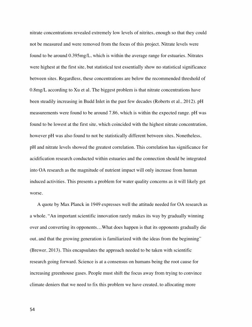
54

nitrate concentrations revealed extremely low levels of nitrites, enough so that they could

not be measured and were removed from the focus of this project. Nitrate levels were

found to be around 0.395mg/L, which is within the average range for estuaries. Nitrates

were highest at the first site, but statistical test essentially show no statistical significance

between sites. Regardless, these concentrations are below the recommended threshold of

0.8mg/L according to Xu et al. The biggest problem is that nitrate concentrations have

been steadily increasing in Budd Inlet in the past few decades (Roberts et al., 2012). pH

measurements were found to be around 7.86, which is within the expected range. pH was

found to be lowest at the first site, which coincided with the highest nitrate concentration,

however pH was also found to not be statistically different between sites. Nonetheless,

pH and nitrate levels showed the greatest correlation. This correlation has significance for

acidification research conducted within estuaries and the connection should be integrated

into OA research as the magnitude of nutrient impact will only increase from human

induced activities. This presents a problem for water quality concerns as it will likely get

worse.

A quote by Max Planck in 1949 expresses well the attitude needed for OA research as

a whole. “An important scientific innovation rarely makes its way by gradually winning

over and converting its opponents…What does happen is that its opponents gradually die

out, and that the growing generation is familiarized with the ideas from the beginning”

(Brewer, 2013). This encapsulates the approach needed to be taken with scientific

research going forward. Science is at a consensus on humans being the root cause for

increasing greenhouse gases. People must shift the focus away from trying to convince

climate deniers that we need to fix this problem we have created, to allocating more

55

attention towards educating younger generations of all the different human causes of OA.

This will promote greater awareness of the problem, and get people thinking about how

to holistically tackle OA in the years to come.

56

References:

Bianucci, L., Long, W., Khangaonkar, T., Pelletier, G., Ahmed, A., Mohamedali, T.,

Roberts, M., Figueroa-Kaminsky, C. (2018). Sensitivity of the regional ocean

acidification and carbonate system in Puget Sound to ocean and freshwater

inputs. Elem Sci Anth,6(1), 22.

Bowen, J. L., & Valiela, I. (2001). The ecological effects of urbanization of coastal

watersheds: Historical increases in nitrogen loads and eutrophication of Waquoit

Bay estuaries. Canadian Journal of Fisheries and Aquatic Sciences, 58(8), 1489-

1500.

Branch, T. A., Dejoseph, B. M., Ray, L. J., & Wagner, C. A. (2013). Impacts of ocean

acidification on marine seafood. Trends in Ecology & Evolution,28(3), 178-186.

Brewer, P. G. (2013). A short history of ocean acidification science in the 20th century:

A chemists view. Biogeosciences Discussions, 10(5), 8715-8748.

Budd Inlet, Olympia Shoal Tides. (2019). Tides.

Busch, S., & Mcelhany, P. (2017). Using mineralogy and higher-level taxonomy as

indicators of species sensitivity to pH: A case-study of Puget Sound. Elem Sci

Anth,5(0), 53.

57

Budd Inlet Scientific Study: An Overview of Findings. (2000). Wastewater Resource

Management Plan, LOTT.

Byrne, M. (2011). Impact of ocean warming and ocean acidification on marine

invertebrate life history stages. Oceanography and Marine Biology

Oceanography and Marine Biology - An Annual Review,49, 1-42.

Carter, H. A., Ceballos-Osuna, L., Miller, N. A., & Stillman, J. H. (2013). Impact of

ocean acidification on metabolism and energetics during early life stages of the

intertidal porcelain crab Petrolisthes cinctipes. Journal of Experimental

Biology,216(8), 1412-1422.

Conductivity, Salinity, & Total Dissolved Solids. Fundamentals of Environmental

Measurements (2014). Fondriest Environmental Learning Center Inc.

Environmental Systems Research Institute (ESRI). Budd Inlet Bathymetry and Sample

Locations. (2019). ArcGIS Online.

Fassbender, A. J., Alin, S. R., Feely, R. A., Sutton, A. J., Newton, J. A., & Byrne, R. H.

(2016). Estimating Total Alkalinity in the Washington State Coastal Zone:

Complexities and Surprising Utility for Ocean Acidification Research. Estuaries

and Coasts, 40(2), 404-418.

58

Fassbender, A. J., Alin, S. R., Feely, R. A., Sutton, A. J., Newton, J. A., Krembs, C.,

Bos, J., Keyzers, M., Devol, A., Ruef, W., Pelletier, G. (2018). Seasonal

carbonate chemistry variability in marine surface waters of the US Pacific

Northwest. Earth System Science Data, 10(3), 1367-1401.

Feely, R. A., Alin, S. R., Newton, J., Sabine, C. L., Warner, M., Devol, A., Krembs, C.,

Maloy, C. (2010). The combined effects of ocean acidification, mixing, and

respiration on pH and carbonate saturation in an urbanized estuary. Estuarine,

Coastal and Shelf Science,88(4), 442-449.

Fine, R. A., Willey, D. A., & Millero, F. J. (2016). Global variability and changes in

ocean total alkalinity from Aquarius satellite data. Geophysical Research

Letters, 44(1), 261-267.

Fry, C. H., Tyrrell, T., Hain, M. P., Bates, N. R., & Achterberg, E. P. (2015). Analysis of

global surface ocean alkalinity to determine controlling processes. Marine

Chemistry, 174, 46-57.

García-Martín, E., Aranguren-Gassis, M., Hartmann, M., Zubkov, M., & Serret,

P. (2017). Contribution of bacterial respiration to plankton respiration from 50°N

to 44°S in the Atlantic Ocean. Progress in Oceanography, 158, 99-108.

59

Hallock, D. (2009). River and stream water quality monitoring report for water year

2008. Olympia, WA: Washington State Dept. of Ecology, Environmental

Assessment Program.

IPACOA Data Explorer. (2019). Integrated Ocean Observing System, Partners

Across Coasts Ocean Acidification.

Kroeker, K. J., Kordas, R. L., Crim, R., Hendriks, I. E., Ramajo, L., Singh, G. S.,

Duarte, C.M.,Gattuso, J. (2013). Impacts of ocean acidification on marine

organisms: Quantifying sensitivities and interaction with warming. Global

Change Biology,19(6), 1884-1896.

Long, W. C., Sant, S. B., Swiney, K. M., & Foy, R. J. (2016). Survival, growth, and

morphology of blue king crabs: Effect of ocean acidification decreases with

exposure time. ICES Journal of Marine Science: Journal Du Conseil.

Long, W. C., Swiney, K. M., Harris, C., Page, H. N., & Foy, R. J. (2013). Effects of

Ocean Acidification on Juvenile Red King Crab (Paralithodes camtschaticus) and

Tanner Crab (Chionoecetes bairdi) Growth, Condition, Calcification, and

Survival. PLoS ONE,8(4).

McCarthy, S., TeMohamedali, T., & Cracknell, P. (2017). Nitrogen in Puget Sound. WA

60

Department of Ecology.

McClelland, J. W., Valiela, I., & Michener, R. H. (1997). Nitrogen-stable isotope

signatures in estuarine food webs: A record of increasing urbanization in coastal

watersheds. Limnology and Oceanography, 42(5), 930-937.

Moore, S., Wold, R., Stark, K., Bos, J., Williams, P., Dzinbal, K., Krembs, C., Newton, J.

(2014). Puget Sound Marine Waters 2014 Overview. NOAA Fisheries.

NOAA: Alaska Fisheries Science Center. (2016). New Studies Raise

Questions About Crabs Adaptability.

NOAA: Pacific Marine Environmental Laboratory (PMEL) (2018). A Primer On pH.

NVS Data Explorer. (2019). Northwest Association of Networked Ocean Observing

Systems (NANOOS).

Roberts, M., Ahmed, A., Pelletier, G. J., & Osterberg, D. (2012). Deschutes River,

Capitol Lake, and Budd Inlet temperature, fecal coliform bacteria, dissolved

oxygen, pH, and fine sediment total maximum daily load technical report: Water

quality study findings (pp. 1-265) (Washington Department of Ecology,

Environmental Assessment Program). Olympia, WA: Washington State Dept. of

Ecology, Environmental Assessment Program.

61

Ocean CO2 uptake – part 2. (2016). And Then There’s Physics, Word Press.

Pelletier, G. J., Laura, B., Wen, L., Tarang, K., Teizeen, M., Anise, A., & Cristiana, F.

(2017). Salish sea model: Ocean acidification module and the response to

regional anthropogenic nutrient sources (pp. 1-90) Washington Department of

Ecology, Environmental Assessment Program.

Reum, J. C., Alin, S. R., Feely, R. A., Newton, J., Warner, M., & Mcelhany, P.

(2014). Seasonal Carbonate Chemistry Covariation with Temperature, Oxygen,

and Salinity in a Fjord Estuary: Implications for the Design of Ocean

Acidification Experiments. PLoS ONE,9(2).

Ries, J. B., Ghazaleh, M. N., Connolly, B., Westfield, I., & Castillo, K. D. (2016).

Impacts of seawater saturation state (ΩA= 0.4–4.6) and temperature (10, 25 °C)

on the dissolution kinetics of whole-shell biogenic carbonates. Geochimica Et

Cosmochimica Acta, 192, 318-337.

Roberts, M., Ahmed, A., Pelletier, G. J., & Osterberg, D. (2012). Deschutes River,

Capitol Lake, and Budd Inlet temperature, fecal coliform bacteria, dissolved

oxygen, pH, and fine sediment total maximum daily load technical report: Water

quality study findings. Olympia, WA: Washington State Dept. of Ecology,

Environmental Assessment Program.

62

Roberts, M., Ahmed, A., & Pelletier, G. J. (2015). Deschutes River, Capitol Lake, and

Budd Inlet total maximum daily load study: Supplemental modeling scenarios (pp.

1-96) Washington State Dept. of Ecology, Environmental Assessment Program.

Rounds, S. (2018). Alkalinity Calculator version 2.22. US Geological Survey, Oregon

Water Science Center.

Rounds, S., & Wilde, F. D. (2012). Alkalinity and acid neutralizing capacity version 4.0.

U.S. Dept. of the Interior, U.S. Geological Survey.

Schnetger, B., & Lehners, C. (2014). Determination of nitrate plus nitrite in small volume

marine water samples using vanadium(III)chloride as a reduction agent. Marine

Chemistry, 160, 91-98.

Sircus, M. (2011). Water, Alkalinity & pH.

Swiney, K. M., Long, W. C., & Foy, R. J. (2017). Decreased pH and increased

temperatures affect young-of-the-year red king crab (Paralithodes

camtschaticus). ICES Journal of Marine Science.

The Chemistry of Ocean Acidification. (2012). Ocean Carbon & Biochemistry.

63

Thurston County Water Resources Monitoring Report, 2016-2017 Water Year. (2018).

Voluntary Estuary Monitoring Manual, Chapter 11: pH and Alkalinity. (2006). US

Environmental Protection Agency. EPA-842-B-06-003.

Wallace, R. B., Baumann, H., Grear, J. S., Aller, R. C., & Gobler, C. J. (2014).

Coastal ocean acidification: The other eutrophication problem. Estuarine, Coastal

and Shelf Science, 148, 1-13.

Wang, S., Cao, L., & Li, N. (2014). Responses of the ocean carbon cycle to

climate change: Results from an earth system climate model simulation. Advances

in Climate Change Research, 5(3), 123-130.

Xu, H., Paerl, H. W., Qin, B., Zhu, G., Hall, N. S., & Wu, Y. (2014). Determining

Critical Nutrient Thresholds Needed to Control Harmful Cyanobacterial Blooms

in Eutrophic Lake Taihu, China. Environmental Science & Technology, 49(2),

1051-1059.

Zeng, X., Chen, X., & Zhuang, J. (2015). The positive relationship between ocean

acidification and pollution. Marine Pollution Bulletin, 91(1), 14-21.

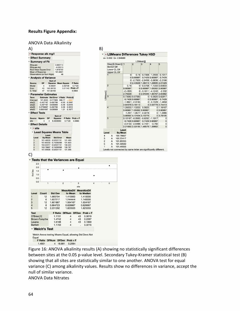
64

Results Figure Appendix: ANOVA Data Alkalinity A) B)

C)

Figure 16: ANOVA alkalinity results (A) showing no statistically significant differences between sites at the 0.05 p-value level. Secondary Tukey-Kramer statistical test (B) showing that all sites are statistically similar to one another. ANOVA test for equal variance (C) among alkalinity values. Results show no differences in variance, accept the null of similar variance. ANOVA Data Nitrates

65

A) B)

C)

Figure 17: ANOVA results (A) for log transformed nitrates showing a statistically significant difference with a p-value of 0.0032, at the 0.05 level. Secondary Tukey-Kramer statistical test (B) showing that site 1 is statistically different from site 3 and 5 for nitrates at the 0.05 level. ANVOA test of equal variance (C). Results show unequal variance between nitrate sites at the 0.05 level. ANOVA Data pH

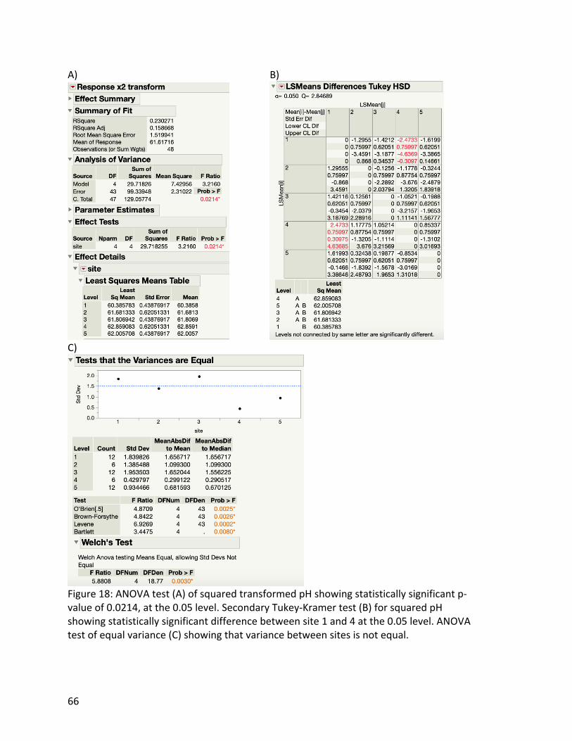
66

A) B)

C)

Figure 18: ANOVA test (A) of squared transformed pH showing statistically significant p-value of 0.0214, at the 0.05 level. Secondary Tukey-Kramer test (B) for squared pH showing statistically significant difference between site 1 and 4 at the 0.05 level. ANOVA test of equal variance (C) showing that variance between sites is not equal.

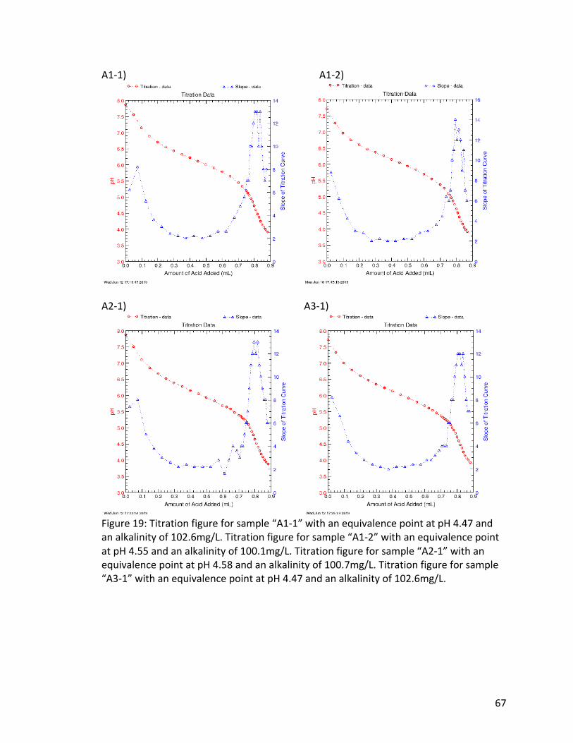
67

A1-1) A1-2)

A2-1) A3-1)

Figure 19: Titration figure for sample “A1-1” with an equivalence point at pH 4.47 and an alkalinity of 102.6mg/L. Titration figure for sample “A1-2” with an equivalence point at pH 4.55 and an alkalinity of 100.1mg/L. Titration figure for sample “A2-1” with an equivalence point at pH 4.58 and an alkalinity of 100.7mg/L. Titration figure for sample “A3-1” with an equivalence point at pH 4.47 and an alkalinity of 102.6mg/L.

68

A3-2) A4-1)

A5-1) A5-2)

Figure 20: Titration figure for sample “A3-2” with an equivalence point at pH 4.68 and an alkalinity of 99.5mg/L. Titration figure for sample “A4-1” with an equivalence point at pH 4.59 and an alkalinity of 101.3mg/L. Titration figure for sample “A5-1” with an equivalence point at pH 4.64 and an alkalinity of 101.3mg/L. Titration figure for sample “A5-2” with an equivalence point at pH 4.51 and an alkalinity of 103.2mg/L.

69

B1-1) B1-2)

B2-1) B3-1)

Figure 21: Titration figure for sample “B1-1” with an equivalence point at pH 4.53 and an alkalinity of 103.2mg/L. Titration figure for sample “B1-2” with an equivalence point at pH 4.46 and an alkalinity of 102.6mg/L. Titration figure for sample “B2-1” with an equivalence point at pH 4.53 and an alkalinity of 103.2mg/L. Titration figure for sample “B3-1” with an equivalence point at pH 4.38 and an alkalinity of 105.7mg/L.

70

B3-2) B4-1)

B5-1) B5-2)

Figure 22: Titration figure for sample “B3-2” with an equivalence point at pH 4.42 and an alkalinity of 103.8mg/L. Titration figure for sample “B4-1” with an equivalence point at pH 4.62 and an alkalinity of 103.2mg/L. Titration figure for sample “B5-1” with an equivalence point at pH 4.63 and an alkalinity of 103.2mg/L. Titration figure for sample “B5-2” with an equivalence point at pH 4.58 and an alkalinity of 101.3mg/L.

71

C1-1) C1-2)

C2-1) C3-1)

Figure 23: Titration figure for sample “C1-1” with an equivalence point at pH 4.64 and an alkalinity of 98.2mg/L. Titration figure for sample “C1-2” with an equivalence point at pH 4.56 and an alkalinity of 99.5mg/L. Titration figure for sample “C2-1” with an equivalence point at pH 4.65 and an alkalinity of 99.5mg/L. Titration figure for sample “C3-1” with an equivalence point at pH 4.67 and an alkalinity of 100.1mg/L.

72

C3-2) C4-1)

C5-1) C5-2)

Figure 24: Titration figure for sample “C3-2” with an equivalence point at pH 4.60 and an alkalinity of 100.7mg/L. Titration figure for sample “C4-1” with an equivalence point at pH 4.47 and an alkalinity of 103.2mg/L. Titration figure for sample “C5-1” with an equivalence point at pH 4.54 and an alkalinity of 99.5mg/L. Titration figure for sample “C5-2” with an equivalence point at pH 4.68 and an alkalinity of 97.6mg/L.