Embed Size (px)
Citation preview
Discriminant Training of Front-End and Acoustic Modeling Stages to
Heterogeneous Acoustic Environments for Multi-stream Automatic
Speech Recognition
by
Michael Lee Shire
B.S. (University of California, San Diego) 1991M.S. (University of California, Berkeley) 1997
A dissertation submitted in partial satisfaction of the
requirements for the degree of
Doctor of Philosophy
in
Engineering - Electrical Engineering and Computer Science
in the
GRADUATE DIVISION
of the
UNIVERSITY OF CALIFORNIA, BERKELEY
Committee in charge:Professor Nelson Morgan, Chair
Professor David WesselProfessor Hynek HermanskyProfessor Jitendra Malik
Professor Steven Greenberg
Fall 2000
The dissertation of Michael Lee Shire is approved:
Chair Date
Date
Date
Date
Date
University of California, Berkeley
Fall 2000
Discriminant Training of Front-End and Acoustic Modeling Stages to
Heterogeneous Acoustic Environments for Multi-stream Automatic
Speech Recognition
Copyright 2000
by
Michael Lee Shire
1
Abstract
Discriminant Training of Front-End and Acoustic Modeling Stages to
Heterogeneous Acoustic Environments for Multi-stream Automatic Speech
Recognition
by
Michael Lee Shire
Doctor of Philosophy in Engineering - Electrical Engineering and Computer Science
University of California, Berkeley
Professor Nelson Morgan, Chair
Automatic Speech Recognition (ASR) still poses a problem to researchers. In particular,
most ASR systems have not been able to fully handle adverse acoustic environments. Al-
though a large number of modi�cations have resulted in increased levels of performance
robustness, ASR systems still fall short of human recognition ability in a large number of
environments. A possible shortcoming of the typical ASR system is the reliance on a single
stream of front-end acoustic features and acoustic modeling feature probabilities. A single
front-end feature extraction algorithm may not be capable of maintaining robustness to
arbitrary acoustic environments. Acoustic modeling will also degrade due to distributional
changes caused by the acoustic environment. This thesis explores the parallel use of mul-
tiple front-end and acoustic modeling elements to improve upon this shortcoming. Each
ASR acoustic modeling component is trained to estimate class posterior probabilities in a
particular acoustic environment. In addition to discriminative training of the probability
estimator, existing feature extraction algorithms are modi�ed in such a way as to improve
class discrimination in the training environment. More speci�cally, Linear Discriminant
Analysis provides a mechanism for obtaining discriminant temporal basis functions that
can replace components of the existing algorithms that were designed in either an em-
pirical or intuitive manner. Probability streams are generated using multiple front-end
acoustic modeling stages trained to heterogeneous acoustic environments. In new sample
acoustic environments, simple combinations of these probability streams give rise to word
2
recognition rates that are superior to the individual streams.
Professor Nelson MorganDissertation Committee Chair
iii
For my mother Arsenia,
my father Arlen
my sister Miriam
and my brother Aaron
iv
Contents
List of Figures vi
List of Tables ix
1 Introduction 1
1.1 Multi-Stream ASR . . . . . . . . . . . . . . . . . . . . . . . . . . . . . . . . 31.2 Acoustic Environments . . . . . . . . . . . . . . . . . . . . . . . . . . . . . . 71.3 Overview . . . . . . . . . . . . . . . . . . . . . . . . . . . . . . . . . . . . . 9
2 Automatic Speech Recognition 11
2.1 Probability Estimation . . . . . . . . . . . . . . . . . . . . . . . . . . . . . . 152.2 Speech Feature Extraction . . . . . . . . . . . . . . . . . . . . . . . . . . . . 17
2.2.1 Time-Frequency Analysis . . . . . . . . . . . . . . . . . . . . . . . . 182.2.2 Feature Orthogonalization . . . . . . . . . . . . . . . . . . . . . . . . 212.2.3 Frequency Smoothing . . . . . . . . . . . . . . . . . . . . . . . . . . 242.2.4 Temporal Processing . . . . . . . . . . . . . . . . . . . . . . . . . . . 262.2.5 Complete Algorithms . . . . . . . . . . . . . . . . . . . . . . . . . . 29
2.3 Acoustic Environments . . . . . . . . . . . . . . . . . . . . . . . . . . . . . . 342.4 Experimental Setup . . . . . . . . . . . . . . . . . . . . . . . . . . . . . . . 39
2.4.1 Speech Corpora . . . . . . . . . . . . . . . . . . . . . . . . . . . . . . 40
3 LDA Temporal Filters for RASTA-PLP 42
3.1 Temporal Filter Design with Linear Discriminant Analysis . . . . . . . . . . 423.2 Temporal LDA Filters in Varying Acoustic Conditions . . . . . . . . . . . . 44
3.2.1 Clean Speech Data . . . . . . . . . . . . . . . . . . . . . . . . . . . . 443.2.2 Reverberated Speech Data . . . . . . . . . . . . . . . . . . . . . . . . 453.2.3 Speech Data With Added Noise . . . . . . . . . . . . . . . . . . . . . 463.2.4 Varying Noise SNR and Reverberation Parameters . . . . . . . . . . 46
3.3 Recognition Results . . . . . . . . . . . . . . . . . . . . . . . . . . . . . . . 513.3.1 Initial Experiments . . . . . . . . . . . . . . . . . . . . . . . . . . . . 513.3.2 Recognition with Local Normalization . . . . . . . . . . . . . . . . . 563.3.3 Performance of Individual LDA Filters . . . . . . . . . . . . . . . . . 61
3.4 Discussion . . . . . . . . . . . . . . . . . . . . . . . . . . . . . . . . . . . . . 64
v
4 LDA temporal �lters with PLP and MSG 68
4.1 Logarithm of the Power Spectra . . . . . . . . . . . . . . . . . . . . . . . . . 684.2 Delta Calculation with Perceptual Linear Prediction . . . . . . . . . . . . . 714.3 Temporal Filtering with the Modulation-Filtered Spectrogram . . . . . . . . 774.4 Discussion . . . . . . . . . . . . . . . . . . . . . . . . . . . . . . . . . . . . . 81
5 Multi-Stream Recognition Tests 85
5.1 Simple Combination Strategies . . . . . . . . . . . . . . . . . . . . . . . . . 865.2 Multi-Stream Experiments with RASTA-PLP . . . . . . . . . . . . . . . . . 90
5.2.1 Combining Heterogeneously Trained MLPs with Identical FeatureProcessing . . . . . . . . . . . . . . . . . . . . . . . . . . . . . . . . . 91
5.2.2 Training an MLP on Data from Two Conditions . . . . . . . . . . . 925.3 RASTA-PLP with Di�erent LDA Filters . . . . . . . . . . . . . . . . . . . . 93
5.3.1 Dual LDA Filter Sets with Common MLP Training Environment . . 945.3.2 Matched LDA Filter and MLP Training Environments . . . . . . . . 96
5.4 PLP and MSG . . . . . . . . . . . . . . . . . . . . . . . . . . . . . . . . . . 995.4.1 Dual-stream PLP and MSG with Common MLP Training Environment1005.4.2 PLP and MSG with Heterogeneously Trained MLPs . . . . . . . . . 1005.4.3 Four Stream Combination . . . . . . . . . . . . . . . . . . . . . . . . 103
5.5 Weighted Stream Combinations . . . . . . . . . . . . . . . . . . . . . . . . . 1045.5.1 Weighting Based on Frame-Level Con�dence . . . . . . . . . . . . . 106
5.6 Final Tests with Unseen Conditions and Best Stream Combination . . . . . 1115.7 Discussion . . . . . . . . . . . . . . . . . . . . . . . . . . . . . . . . . . . . . 115
6 Conclusion 119
6.1 Discriminant Feature Extraction . . . . . . . . . . . . . . . . . . . . . . . . 1206.2 Multi-Stream Combinations . . . . . . . . . . . . . . . . . . . . . . . . . . . 1216.3 Contribution and Future Work . . . . . . . . . . . . . . . . . . . . . . . . . 123
A Recognition Units 125
B Temporal LDA Filters with Phonetic Units 128
C Temporal LDA Filters with Syllabic Units 132
D Temporal LDA Filters for PLP 135
E Correlating Frame Accuracy and Word Error 137
E.1 Method . . . . . . . . . . . . . . . . . . . . . . . . . . . . . . . . . . . . . . 138E.2 Experiments . . . . . . . . . . . . . . . . . . . . . . . . . . . . . . . . . . . . 139E.3 Discussion . . . . . . . . . . . . . . . . . . . . . . . . . . . . . . . . . . . . . 147
Bibliography 148
vi
List of Figures
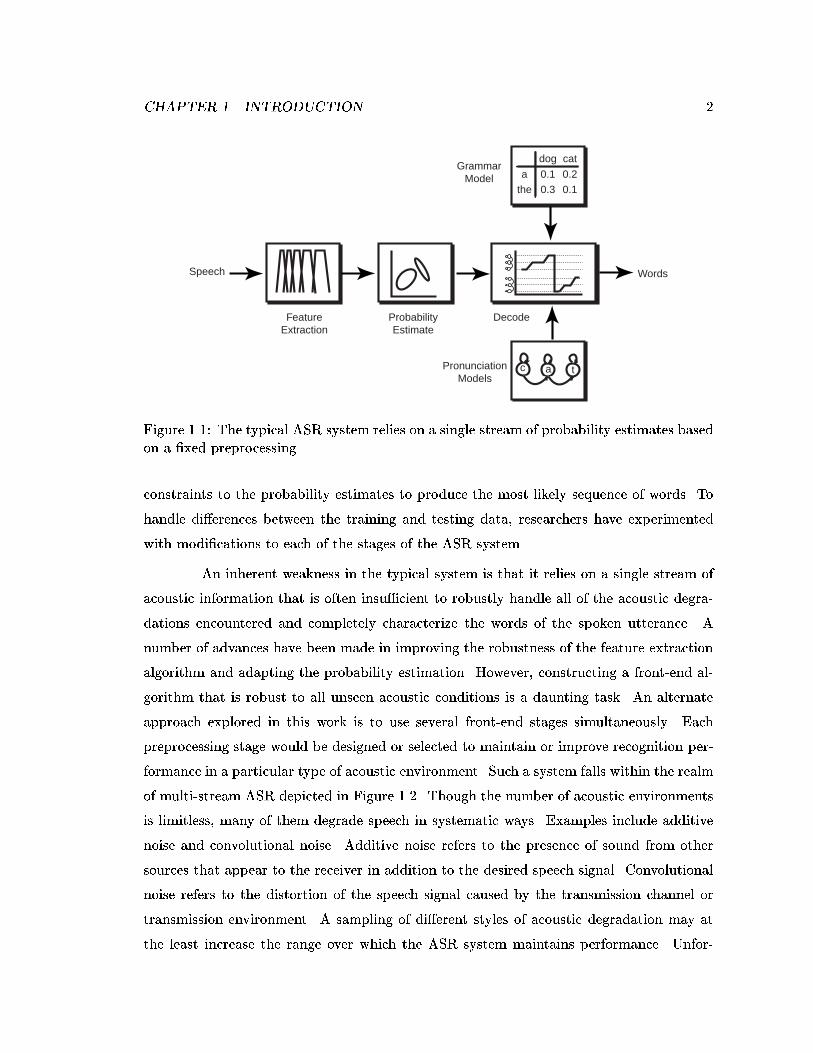
1.1 The typical ASR system relies on a single stream of probability estimatesbased on a �xed preprocessing. . . . . . . . . . . . . . . . . . . . . . . . . . 2
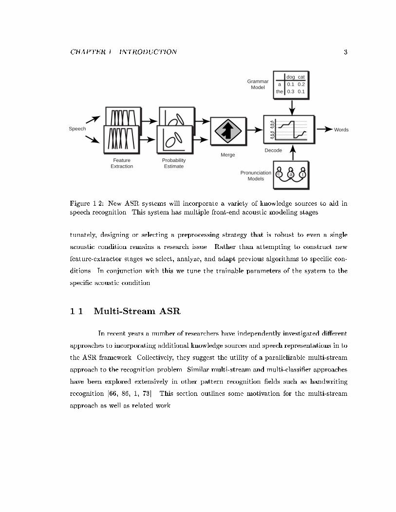
1.2 New ASR systems will incorporate a variety of knowledge sources to aid inspeech recognition. This system has multiple front-end acoustic modelingstages. . . . . . . . . . . . . . . . . . . . . . . . . . . . . . . . . . . . . . . . 3
1.3 Speech features from di�erent acoustic environments can exhibit di�erentfeature distributions. . . . . . . . . . . . . . . . . . . . . . . . . . . . . . . . 7
1.4 In addition to the non-linear discrimination used in the MLP along thefrequency-related dimension, we apply discriminant training along the timedimension. . . . . . . . . . . . . . . . . . . . . . . . . . . . . . . . . . . . . . 8
2.1 Abstract depiction of a typical ASR system. . . . . . . . . . . . . . . . . . . 122.2 Hidden Markov Model. . . . . . . . . . . . . . . . . . . . . . . . . . . . . . . 132.3 Fully connected multi-layer perceptron. . . . . . . . . . . . . . . . . . . . . 162.4 Integration windows of critical-band-like ranges spaced at 1 Bark intervals. 202.5 Dimensions of maximum variance and linear separability may not coincide. 242.6 Impulse and frequency response for standard RASTA �lter. . . . . . . . . . 282.7 Processing steps for RASTA-PLP. . . . . . . . . . . . . . . . . . . . . . . . 302.8 Processing steps for the MSG features. . . . . . . . . . . . . . . . . . . . . . 322.9 Processing diagram for online normalization. . . . . . . . . . . . . . . . . . 342.10 Processing schematic for AGC. . . . . . . . . . . . . . . . . . . . . . . . . . 352.11 Log-power trajectory of 3 seconds of the same utterance under the original
clean condition, with added factory noise at 10 dB SNR, and lightly reverber-ated with a characteristic reverberation time of 0.5 seconds. The utteranceis of a male speaker saying \Well, uh, maybe I should tell ya about how..." 35
2.12 Log-power trajectory of same utterance as in Figure 2.11 under severelyreverberated condition (characteristic reverberation time of 2.5 seconds). . . 36
2.13 Average spectral power for car and factory noise. . . . . . . . . . . . . . . . 38
3.1 LDA is applied to the temporal trajectories of the log-critical-band energy.Linguistic classes are assigned to the center of relatively long time spanningwindows of trajectories. Means � and covariances � are collected for eachclass. . . . . . . . . . . . . . . . . . . . . . . . . . . . . . . . . . . . . . . . . 43
vii
3.2 Averaged impulse and frequency responses for LDA �lters derived with cleandata. . . . . . . . . . . . . . . . . . . . . . . . . . . . . . . . . . . . . . . . . 45
3.3 Impulse and frequency responses for averaged LDA �lters derived with re-verberated data. . . . . . . . . . . . . . . . . . . . . . . . . . . . . . . . . . 47
3.4 Impulse and frequency responses for �lters derived from speech data withadded noise. . . . . . . . . . . . . . . . . . . . . . . . . . . . . . . . . . . . . 48
3.5 Impulse and frequency responses for �lters derived with varying car noiseSNR, reverberation T60, reverberation DTR, and reverberation T60 andDTR. . . . . . . . . . . . . . . . . . . . . . . . . . . . . . . . . . . . . . . . 50
3.6 Impulse and frequency responses when varying the proportion of clean andheavy reverberated training data. . . . . . . . . . . . . . . . . . . . . . . . . 52
3.7 The RASTA �lter is replaced by �lters derived from LDA based on theStories corpus. Recognition tests used the Numbers corpus. . . . . . . . . 53
3.8 Feature distributions from speech distorted by environmental conditions canbe warped to match an undistorted distribution. . . . . . . . . . . . . . . . 57
3.9 Examples of the histogram distribution of �rst cepstral coe�cient for PLPand RASTA-PLP before and after per-utterance local normalization. . . . . 58
4.1 Histogram distributions of the critical-band output centered at 570 Hz, andsubjected to cube-root, eighth-root and logarithmic compression. The dis-tributions are for the phones /ow/, /eh/, /n/, /r/, /s/, and /k/. Rangesand densities are scaled individually for comparison. . . . . . . . . . . . . . 69
4.2 Skewness and Kurtosis statistics of the critical-band output centered at 570Hz, and subjected to cube root, eighth root, and logarithm for the phones/ow/, /eh/, /n/, /r/, /s/, and /k/. . . . . . . . . . . . . . . . . . . . . . . . 70
4.3 The delta calculation for PLP is replaced by temporal �lters derived fromLDA . . . . . . . . . . . . . . . . . . . . . . . . . . . . . . . . . . . . . . . . 75
4.4 Histogram distributions of the �rst, fourth, and seventh PLP cepstral coef-�cient. The distributions are for the phones /ow/, /eh/, /n/, /r/, /s/, and/k/. Ranges and densities are scaled individually for comparison. . . . . . . 76
4.5 The lowpass and bandpass �lters in MSG are replaced by �lters derivedusing LDA. . . . . . . . . . . . . . . . . . . . . . . . . . . . . . . . . . . . . 77
4.6 The fundamental frequency of the input remains after application of a non-linearity, but with added harmonics. . . . . . . . . . . . . . . . . . . . . . . 78
4.7 Di�erence between the frame accuracy of individual phones for MSG withand without LDA �lters. Positive bars indicate MSG-LDA had higher frameaccuracy. . . . . . . . . . . . . . . . . . . . . . . . . . . . . . . . . . . . . . 82
5.1 Comparison of RASTA-PLP with LDA-RASTA-PLP using average and log-average posterior combination. Signi�cant improvement is marked with anarrow. . . . . . . . . . . . . . . . . . . . . . . . . . . . . . . . . . . . . . . . 99
5.2 Frame accuracy and WER for a range of arti�cial reverberant conditions us-ing a weighted log-average between two LDA-RASTA-PLP streams trainedon clean and heavy reverberation data. Tests performed on room impulseswith DTR = -8 dB. . . . . . . . . . . . . . . . . . . . . . . . . . . . . . . . 105
viii
5.3 Frame accuracy and WER for a range of arti�cial reverberant conditions us-ing a weighted log-average between two LDA-RASTA-PLP streams trainedon clean and heavy reverberation data. Tests performed on room impulseswith T60 = 2 sec. . . . . . . . . . . . . . . . . . . . . . . . . . . . . . . . . 106
5.4 Frame accuracy and WER for a range of arti�cial reverberant conditionsusing a weighted log-average between PLP and MSG streams trained onclean and heavy reverberation data respectively. Tests performed on roomimpulses with DTR = -8 dB. . . . . . . . . . . . . . . . . . . . . . . . . . . 107
5.5 Frame accuracy and WER for a range of arti�cial reverberant conditionsusing a weighted log-average between PLP and MSG streams trained onclean and heavy reverberation data respectively. Tests performed on roomimpulses with T60 = 2 sec. . . . . . . . . . . . . . . . . . . . . . . . . . . . 107
B.1 Impulse and frequency responses for �rst three LDA �lters derived withclean data. . . . . . . . . . . . . . . . . . . . . . . . . . . . . . . . . . . . . . 129
B.2 Impulse and frequency responses for �rst three LDA �lters derived withheavy reverberated data. . . . . . . . . . . . . . . . . . . . . . . . . . . . . . 130
B.3 Impulse and frequency responses for �rst three LDA �lters derived withfactory noise data at 10 dB SNR. . . . . . . . . . . . . . . . . . . . . . . . . 131
C.1 First three LDA �lters derived with syllable targets on clean data. . . . . . 133C.2 Comparison of averaged �lters using syllable targets in di�erent noise con-
ditions. . . . . . . . . . . . . . . . . . . . . . . . . . . . . . . . . . . . . . . 134
D.1 First three LDA �lters derived from PLP cepstra on clean data. . . . . . . . 136
E.1 Histogram of WER for 500 recognition runs. In each run random incorrectframes were corrected to yield a frame accuracy of 70%. . . . . . . . . . . . 139
E.2 WER for one recognition run of randomly chosen corrected frames wherethe value of the posterior placed corrected frames was varied. . . . . . . . . 140
E.3 WER for 20 recognition runs with a varying proportion of corrected silenceframes. . . . . . . . . . . . . . . . . . . . . . . . . . . . . . . . . . . . . . . . 141
E.4 WER for 20 recognition runs with a varying proportion of vowel framescorrected. . . . . . . . . . . . . . . . . . . . . . . . . . . . . . . . . . . . . . 143
E.5 WER for 20 recognition runs with a varying proportion of vowel framescorrected. All silence frames were corrected independently. . . . . . . . . . . 143
E.6 WER for 20 recognition runs with a varying proportion of vowel framescorrected. All incorrect silence frames were left uncorrected. . . . . . . . . . 144
E.7 WER for 20 recognition runs with a varying proportion of the correctedframes that bordered phone transitions in the hand transcription of theNumbers corpus. . . . . . . . . . . . . . . . . . . . . . . . . . . . . . . . . . 145
E.8 WER for 20 recognition runs with a varying proportion of the correctedframes that were within 2 frames from phone transitions in the hand tran-scription of the Numbers corpus. . . . . . . . . . . . . . . . . . . . . . . . . 146
ix
List of Tables
2.1 Description of noise conditions. . . . . . . . . . . . . . . . . . . . . . . . . . 38
3.1 Frame accuracy results using RASTA-PLP, preliminary tests. . . . . . . . . 543.2 Word recognition results using RASTA-PLP, preliminary tests. . . . . . . . 543.3 Frame accuracy results using LDA-RASTA-PLP, preliminary tests. The
+(-) annotatations mark signi�cantly better(worse) performance thanRASTA-PLP without LDA in Table 3.1. . . . . . . . . . . . . . . . . . . . . 55
3.4 Word recognition results using LDA-RASTA-PLP, preliminary tests. The+(-) annotatations mark signi�cantly better(worse) performance thanRASTA-PLP without LDA in Table 3.2. . . . . . . . . . . . . . . . . . . . . 55
3.5 Frame accuracy results using RASTA-PLP, with per-utterance normalization. 593.6 Word recognition results using RASTA-PLP, with per-utterance normaliza-
tion. . . . . . . . . . . . . . . . . . . . . . . . . . . . . . . . . . . . . . . . . 593.7 Frame accuracy results using LDA-RASTA-PLP, with per-utterance nor-
malization. The +(-) annotatations mark signi�cantly better (worse) per-formance than RASTA-PLP without LDA in Table 3.5. . . . . . . . . . . . 60
3.8 Word recognition results using LDA-RASTA-PLP, with per-utterance nor-malization. The +(-) annotatations mark signi�cantly better (worse) per-formance than RASTA-PLP without LDA in Table 3.6. . . . . . . . . . . . 60
3.9 Frame accuracy using LDA �lters derived from reverberant data and anMLP with a single frame of input features. The +(-) annotations markwhere results using the light and heavy �lters are signi�cantly better (worse)than when using the clean �lter. . . . . . . . . . . . . . . . . . . . . . . . . 63
3.10 WER using LDA �lters derived from reverberant data and an MLP witha single frame of input features. The +(-) annotations mark where resultsusing the light and heavy �lters are signi�cantly better (worse) than whenusing the clean �lter. . . . . . . . . . . . . . . . . . . . . . . . . . . . . . . . 63
3.11 Frame accuracy using LDA �lters derived with reverberant data and MLPcontext window of 9 frames. . . . . . . . . . . . . . . . . . . . . . . . . . . . 65
3.12 WER using LDA �lters derived with reverberant data and MLP contextwindow of 9 frames. . . . . . . . . . . . . . . . . . . . . . . . . . . . . . . . 65
x
4.1 Frame accuracy results using PLP with per-utterance normalization. The+(-) annotations mark where the performance is signi�cantly better(worse)than the RASTA-PLP with per-utterance normalization in Table 3.5. . . . 72
4.2 Word recognition results using PLP with per-utterance normalization. The+(-) annotations mark where the performance is signi�cantly better(worse)than the RASTA-PLP with per-utterance normalization in Table 3.6. . . . 72
4.3 Comparison of PLP with delta features and PLP with LDA �lters. MLP wastrained with single frame context of acoustic features. The +(-) annotationsmark where PLP with the LDA is signi�cantly better(worse) than PLP with�s. . . . . . . . . . . . . . . . . . . . . . . . . . . . . . . . . . . . . . . . . . 74
4.4 Comparison of original MSG and MSG with LDA-derived �lters. MLPtrained on acoustic context of 9 frames. The +(-) annotations mark wherethe MSG with LDA �lters is signi�cantly better(worse) than the originalMSG. . . . . . . . . . . . . . . . . . . . . . . . . . . . . . . . . . . . . . . . 80
4.5 Frame accuracy and WER with corrected silence phones for MSG and MSG-LDA. . . . . . . . . . . . . . . . . . . . . . . . . . . . . . . . . . . . . . . . . 83
5.1 Results when combining two trained MLPs at the frame level. One MLPis trained with clean data and the other with heavy reverberation data.RASTA-PLP features were used for both conditions. The \+" annotationsmark where the combinations in the unseen light reverberation testing caseare signi�cantly better than both of the singly trained MLPs. . . . . . . . . 91
5.2 Word error results with a single MLP with twice the number of parameterstrained with clean data, heavy reverberation data, and both. . . . . . . . . . 92
5.3 WER Results from a frame-level combination of LDA-RASTA-PLP withLDA �lters derived under clean and heavy reverberation conditions. TheMLP probability estimator was trained with clean data and a single frameof acoustic features. The \+" annotations mark where the combinations arebetter than the single streams. . . . . . . . . . . . . . . . . . . . . . . . . . 95
5.4 WER Results from a frame-level combination of LDA-RASTA-PLP withLDA �lters derived under clean and heavy reverberation conditions. TheMLP probability estimator was trained with light reverberation data anda single frame of acoustic features. The \+" annotations mark where thecombinations are better than the single streams. . . . . . . . . . . . . . . . 95
5.5 WER Results from a frame-level combination of LDA-RASTA-PLP withLDA �lters derived under clean and heavy heavy reverberation conditions.The MLP probability estimator was trained with heavy reverberation
data and a single frame of acoustic features. The \+" annotations markwhere the combinations are better than the single streams. . . . . . . . . . 95
5.6 WER Results from a frame-level combination of LDA-RASTA-PLP withLDA �lters derived under clean and heavy reverberation conditions. TheMLP probability estimator was trained with clean data and a context win-dow of 9 frames. The \+" annotations mark where the combinations arebetter than the single streams. . . . . . . . . . . . . . . . . . . . . . . . . . 97
xi
5.7 WER Results from a frame-level combination of LDA-RASTA-PLP withLDA �lters derived under clean and heavy reverberation conditions. TheMLP probability estimator was trained with light reverberation data anda context window of 9 frames. The \+" annotations mark where the com-binations are better than the single streams. . . . . . . . . . . . . . . . . . 97
5.8 WER Results from a frame-level combination of LDA-RASTA-PLP withLDA �lters derived under clean and heavy reverberation conditions. TheMLP probability estimator was trained with heavy reverberation dataand a context window of 9 frames. The \+" annotations mark where thecombinations are better than the single streams. . . . . . . . . . . . . . . . 97
5.9 Results from a frame-level combination of LDA-RASTA-PLP with LDA �l-ters and an MLP trained under clean and heavy reverberation. The MLPhad a single frame of acoustic features as input. The \+" annotation markswhere the combination is signi�cantly better than the single streams in thelight reverberation test. . . . . . . . . . . . . . . . . . . . . . . . . . . . . . 98
5.10 Results from a frame-level combination of LDA-RASTA-PLP with LDA �l-ters and an MLP trained under clean and heavy reverberation. The MLPhad an acoustic context of 9 frames. The \+" annotation marks wherethe combination is signi�cantly better than the single streams in the light
reverberation test. . . . . . . . . . . . . . . . . . . . . . . . . . . . . . . . . 985.11 WER Results from a frame-level combination of PLP and MSG with MLP
probability estimators trained with clean data. The \+" annotation markswhere the combination is signi�cantly better than the single streams. . . . . 101
5.12 WER Results from a frame-level combination of PLP and MSG with MLPprobability estimators trained with light reverberation data. The \+"annotation marks where the combination is signi�cantly better than thesingle streams. . . . . . . . . . . . . . . . . . . . . . . . . . . . . . . . . . . 101
5.13 WER Results from a frame-level combination of PLP and MSG with MLPprobability estimators trained with heavy reverberation data. The \+"annotation marks where the combination is signi�cantly better than thesingle streams. . . . . . . . . . . . . . . . . . . . . . . . . . . . . . . . . . . 101
5.14 WER Results from a frame-level combination of PLP with its MLP trainedon clean data and MSG with its MLP probability estimators trained withheavy reverberation data. The \+" annotation marks where the combina-tion is signi�cantly better than the single streams in the light reverberationtest. . . . . . . . . . . . . . . . . . . . . . . . . . . . . . . . . . . . . . . . . 102
5.15 WER Results from a frame-level combination of PLP-LDA with its LDA�lters and MLP trained on clean data and MSG-LDA with its LDA �ltersand MLP probability estimators trained with heavy reverberation data.The \+" annotation marks where the combination is signi�cantly betterthan the single streams in the light reverberation test. . . . . . . . . . . . . 102
5.16 Comparison of frame accuracies for PLP with MSG combinations with andwithout LDA. The \+" annotation marks where the frame accuracy usingLDA augmentation is signi�cantly better than the original. . . . . . . . . . 103
xii
5.17 Four stream combination: PLP and MSG using both clean and heavy rever-beration trained MLPs. The \+" annotation marks where the combinationis signi�cantly better than the single streams in the light reverberation test. 103
5.18 WER Results from a frame-level weighted log-average combination of LDA-RASTA-PLP with clean and heavy trained MLP and LDA �lters using con-�dence based weighting. MLPs were trained with a single input frame offeatures. The \+" and \-" annotations mark two cases where the weightingproduced WER that was respectively signi�cantly better and worse than theequal weighting. . . . . . . . . . . . . . . . . . . . . . . . . . . . . . . . . . . 111
5.19 Final tests using four PLP and MSG streams trained in clean and heavy
reverberation. Combination using log-average posteriors with equal weight-ing. The +(-) annotations mark where the log-average posterior mergingproduced WER that was signi�cantly better (worse) than the single streams. 112
5.20 Combination of four PLP and MSG streams trained in clean and heavy re-verberation with unequal weighting. Two clean streams weighted at 0.1 andheavy reverberation streams weighted at 0.4. The \+" annotations markwhere the log-average posterior merging produced WER that was signi�-cantly lower than the single streams. . . . . . . . . . . . . . . . . . . . . . 113
5.21 Final tests using four PLP and MSG streams trained in clean and the mod-erately heavy reverberation room impulse from the last row. Combinationsused log-average posteriors with speci�ed weighting. The + annotationsmark where the log-average posterior merging produced WER that was sig-ni�cantly lower than the single streams. . . . . . . . . . . . . . . . . . . . . 114
A.1 Words contained in the subset of the OGI Numbers corpus used for wordrecognition experiments. . . . . . . . . . . . . . . . . . . . . . . . . . . . . . 126
A.2 Set of phone classes used in ICSI recognition system. . . . . . . . . . . . . . 127
xiii
Acknowledgments
This dissertation encompasses work from the �nal years of my graduate studies and was
principally funded by the International Computer Science Institute (ICSI) and NSF Grant
IRI-9712579. It would not have been possible were it not for many relationships with
colleagues and friends that I developed and for which I am deeply grateful.
I am very much indebted to my advisor Nelson Morgan for his continual patronage,
support and guidance over the span of my stay at U.C. Berkeley and ICSI. I consider myself
extremely fortunate to have had an advisor who is approachable and always with practical
advise, and who has been a reliable advocate for his students.
I would like to thank Steven Greenberg. I am continually impressed by his scholar-
ship and extensive knowledge of literature regarding many aspects of audition and speech.
His keen insights and attention to detail have constantly provided a sanity check for my
work.
I would like to express my gratitude to Hynek Hermansky for his contagious
enthusiasm and for the advisorial role he undertook while I conducted this research. Much
of this dissertation owes to the excellent research by him and his students at the Oregon
Graduate Institute (OGI). I would like to also acknowledge Narenderath Malayath, Sachin
Kajarekar, Sangita Sharma, Sarel van Vuuren, and Carlos Avendan~no from OGI for their
helpful discussions.
I would like to thank David Wessel and Jitendra Malik for pleasantly serving on
my thesis committee. I would also like to thank Jitendra Malik, Robert Brodersen, and
Charles Stone for serving on my qualifying exam committee.
I conducted this research as a member of the ICSI Realization Group. ICSI
provided a wonderful and rewarding environment for research. I am blessed to have been
able to work alongside many gifted and supportive colleagues. I would like to acknowledge
and thank the many members, past and present, who have all directly and indirectly
contributed to my work in countless ways. Thanks go to Krste Asanovic, Jim Beck, Herv�e
Bourlard, Michael Berthold, Shawn Chang, David Gelbart, Dan Gildea, Ben Gold, Andy
Hatch, Joy Hollenback, Adam Janin, Dan Jurafsky, Yochai Konig, Kristine Ma, Nikki
Mirghafori, Liz Schriberg, Rosaria Silipo, Andreas Stolcke, Gary Tajchman, Grace Tong,
Warner Warren, Chuck Wooters, and Geo� Zweig. I'd like to give additional thanks to
Brian Kingsbury, who provided me with reverberation material for my thesis; to Su-Lin
xiv
Wu, who provided the focus application for my early work with syllable-onset detection;
to Barry Chen, my faithful Paduan learner and o�ce mate, who helped me with many
recent projects; to Eric Fosler-Lussier, the quintessential UNIX guru who kindly tolerated
even my most inane system questions; and to Dan Ellis and Je� Bilmes, brilliant, pleasant
and proli�c researchers and coders whose contributions to the ICSI speech software greatly
facilitated my experiments. I have also bene�ted from help and interactions with Markham
Dickey, Jane Edwards, Lila Finhill, David Johnson, Diane Pokorny, Maria Quintana the
rest of the ICSI administrative sta�.
As ICSI is an international research facility, I have had the privilege of meeting
many international visitors. I would like to acknowledge Toshihiko Abe, Carmen Benitez,
Stephane DuPont, Philipp Faerber, Javier Ferreiros Lopez, Jean Hennebert, Katrin Kirch-
ho�, Rainer Klisch, Hiroaki Ogawa, Florien Schiel, and Mirjam Wester for their friendly
discussions. I'd like to give special thanks to Dominique Genoud and his family for their
friendship and excellent wine. I also wish to express special appreciation to Takayuki Arai
for his hospitality during my visits to his lab at Sophia University and to the members
of his lab, especially Yuji Murahara and Akiko Kusumoto. I was also very fortunate to
have spent several months on loan to Siemens ZT, AG in Munich and wish to thank my
colleagues there, especially Josef Bauer, Joachim K�ohler and Alfred Hauenstein.
I would lastly like to express my appreciation to my other friends and colleagues
outside my �eld of specialization. Among my friends in the EECS department, special
thanks go to Ron Galicia, Lillian Chu, Bill Chen, Tim Calahan, Nimish Shah, and Ruth
Gjerde (the amiable interface between grad student and department). My community
awareness and grad-school experience were signi�cantly enhanced while I was a member
and later principal coordinator of pangit and I am grateful to its former members. I am
especially grateful to John Scott, the nuclear engineering bartender; Irene Soriano, always
concerned with my social welfare; Jody and Marivi Blanco, with whom conversation was
inexorably interesting; and Anatalio Ubalde, the consummate politician. Thanks also go
to Maria Bates, Amanda Camposagrado, Glen Fajardo, Evelyn Rodriguez, and Erlene
Schar�. My graduate school experience would have been neither enjoyable nor endurable
were it not for these and other many friendships that I developed while at Berkeley.
Finally, I'd like to give my thanks to my many friends in San Diego and my love
and thanks to my mother, father, sister, and brother who have all waited patiently for my
life to begin.
1
Chapter 1
Introduction
For the past several decades, researchers have sought ways to automatically recog-
nize and transcribe speech by machine. Continually improving techniques have raised the
state of the art to achieving low error rates on a variety of tasks. Despite many advances,
automatic speech recognition (ASR) still falls far short of the capability of humans [72].
This is often attributed to mismatches between the test material and the data used to
train the recognizer. The mismatches are generally attributed to causes such as di�erent
environmental conditions and di�ering speaker characteristics. Because human recognition
is typically much better in a wide range of acoustic environmental conditions, some of the
problems may lie with how speech is analyzed and represented.
The typical ASR system proceeds along a single acoustic stream approach shown
in Figure 1.11 . First, a signal processing module extracts features from the speech. In Hid-
den Markov Model (HMM) systems or hybrid Arti�cial Neural Network - Hidden Markov
Model (ANN-HMM) based systems, probabilities that a given set of generated features
correspond to particular sub-word units are estimated and fed into the decoder. In Gaus-
sian mixture model (GMM) systems the likelihood that the features are generated by a
particular sub-word unit is estimated and used by the decoder2. The feature extraction
and probability estimation are commonly referred to as the front-end and acoustic mod-
eling components of the ASR system. The decoder applies word models and grammar
1This �gure is an abstraction only; many systems have integrated some of these components and pa-rameters. However, the principle is the same.
2Actually, scaled probabilities (whether posteriors from ANNs or likelihoods from GMMs) are commonlyused in the decoding.
CHAPTER 1. INTRODUCTION 2
dog cat
a
the
0.1
0.3
0.2
0.1
FeatureExtraction
ProbabilityEstimate
Decode
Speech Words
PronunciationModels
GrammarModel
c a t
Figure 1.1: The typical ASR system relies on a single stream of probability estimates basedon a �xed preprocessing.
constraints to the probability estimates to produce the most likely sequence of words. To
handle di�erences between the training and testing data, researchers have experimented
with modi�cations to each of the stages of the ASR system.
An inherent weakness in the typical system is that it relies on a single stream of
acoustic information that is often insu�cient to robustly handle all of the acoustic degra-
dations encountered and completely characterize the words of the spoken utterance. A
number of advances have been made in improving the robustness of the feature extraction
algorithm and adapting the probability estimation. However, constructing a front-end al-
gorithm that is robust to all unseen acoustic conditions is a daunting task. An alternate
approach explored in this work is to use several front-end stages simultaneously. Each
preprocessing stage would be designed or selected to maintain or improve recognition per-
formance in a particular type of acoustic environment. Such a system falls within the realm
of multi-stream ASR depicted in Figure 1.2. Though the number of acoustic environments
is limitless, many of them degrade speech in systematic ways. Examples include additive
noise and convolutional noise. Additive noise refers to the presence of sound from other
sources that appear to the receiver in addition to the desired speech signal. Convolutional
noise refers to the distortion of the speech signal caused by the transmission channel or
transmission environment. A sampling of di�erent styles of acoustic degradation may at
the least increase the range over which the ASR system maintains performance. Unfor-
CHAPTER 1. INTRODUCTION 3
dog cat
a
the
0.1
0.3
0.2
0.1
FeatureExtraction
ProbabilityEstimate
Decode
Speech Words
PronunciationModels
GrammarModel
c a t
Merge
Figure 1.2: New ASR systems will incorporate a variety of knowledge sources to aid inspeech recognition. This system has multiple front-end acoustic modeling stages.
tunately, designing or selecting a preprocessing strategy that is robust to even a single
acoustic condition remains a research issue. Rather than attempting to construct new
feature-extractor stages we select, analyze, and adapt previous algorithms to speci�c con-
ditions. In conjunction with this we tune the trainable parameters of the system to the
speci�c acoustic condition.
1.1 Multi-Stream ASR
In recent years a number of researchers have independently investigated di�erent
approaches to incorporating additional knowledge sources and speech representations in to
the ASR framework. Collectively, they suggest the utility of a parallelizable multi-stream
approach to the recognition problem. Similar multi-stream and multi-classi�er approaches
have been explored extensively in other pattern recognition �elds such as handwriting
recognition [66, 86, 1, 73]. This section outlines some motivation for the multi-stream
approach as well as related work.
CHAPTER 1. INTRODUCTION 4
Redundant Representations in the Human Auditory System
Just as speech is highly redundant, there is evidence to suggest that the human
auditory system is also highly redundant [85, 37]. Numerous perceptual experiments have
been conducted which systematically degrade speech in a variety of ways but where intelligi-
bility was not signi�cantly impaired. Such experiments include extreme low- and high-pass
�ltering of the speech signal [33, 2], �ltering modulation energies [26, 5, 4], desynchro-
nizing speech energy channels [44, 105], and minimizing spectral cues [40, 97, 72]. These
experiments and many others suggest a redundancy in acoustic representation within the
human auditory system such that when one or more representations are corrupted, enough
additional representations remain robust enough to successfully decode the speech. Various
physiological evidence suggests that the primary auditory cortex contains an elegant col-
lection of repeated representations of the acoustic spectro-temporal information at various
scales [112, 96, 39]. This redundancy of multi-scale representations is a key component in
the ability of humans to recognize spoken utterances in acoustically adverse environments.
For ASR systems to attain such robustness, it will probably be necessary to incorporate
this style of multiple representations within the ASR framework.
Multiple Knowledge Sources
In terms of an engineering solution to the ASR problem, many researchers have
already investigated incorporating additional knowledge sources into recognition systems.
For example:
� Combined auditory and visual systems have been proposed for ASR improvement
[77, 22, 16, 15]. Bregler and associates have used visual features from a lip-reading
system to improve performance on a letter recognition task [14, 13].
� Segmental information derived from the speech has been successfully used as an
additional knowledge source [120, 53].
� Wu and associates have successfully experimented with the incorporation of syllabic
units in addition to phonetic units within the ASR framework [118, 117].
CHAPTER 1. INTRODUCTION 5
Combinations of Specialized Preprocessing
The feature extraction process has been continually re�ned over the years resulting
in preprocessing systems that include perceptually inspired analysis and noise robustness
(J-RASTA-PLP3 for example [67]). However, some have developed other preprocessing
strategies based on alternate criteria. For instance, modulation spectral features that an-
alyze longer time windows and display some invariance to reverberant conditions were
developed by Kingsbury and Greenberg [62, 43]. Bilmes developed modulation correlation
based features that capture some of the joint spectro-temporal distribution information
[7]. Others have investigated the use of wavelet based features which provide some multi-
resolution analysis of the speech, for example [112, 96]. Alone, these techniques provide
encouraging recognition results. However, when some are combined with the more tradi-
tional feature extraction approaches such as Mel Cepstra and PLP, results improve even
further, particularly when testing under conditions other than those originally trained on
[7, 61]. This suggests that the alternate preprocessing strategies, though containing much
overlapping information with the \standard" approaches, also contain information about
speech cues that are not contained in the standard preprocessing or that may be more
robust to a di�erent set of adverse conditions.
Ensemble of Classi�ers
In addition to supporting separate feature extraction procedures, researchers have
frequently found advantages to supporting multiple classi�ers. The multiple classi�ers can
operate on either identical, disjoint, or distinct but overlapping sets of classes and features.
Some previous work involving multiple classi�ers includes the following.
� Multiple classi�ers have been used in speaker veri�cation [100]. In speaker recognition
task, arrays of binary classi�ers have been used to distinguish hierarchically among
speakers, for example in [18, 88].
� In multi-band analysis, the frequency space is partitioned into separate ranges and a
separate classi�er operates on each range to produce multiple probability estimates.
This has been shown to reduce performance loss due to frequency localized noise
3RelAtive SpecTrAl - Perceptual Linear Prediction
CHAPTER 1. INTRODUCTION 6
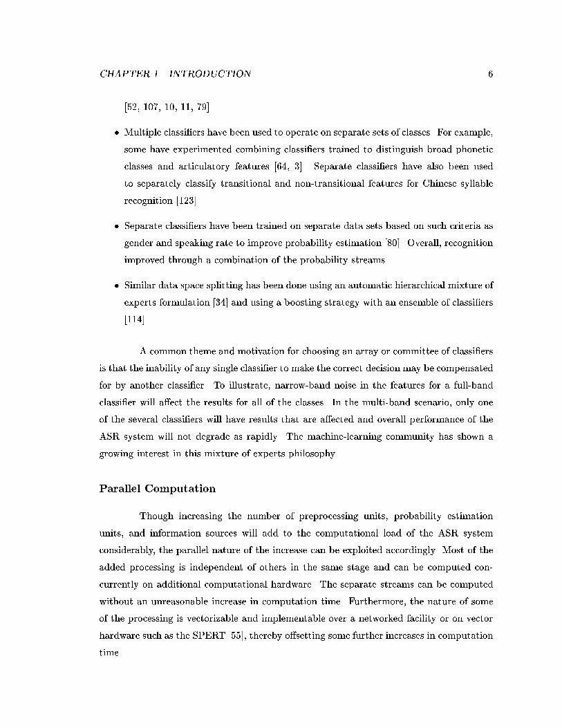
[52, 107, 10, 11, 79].
� Multiple classi�ers have been used to operate on separate sets of classes. For example,
some have experimented combining classi�ers trained to distinguish broad phonetic
classes and articulatory features [64, 3]. Separate classi�ers have also been used
to separately classify transitional and non-transitional features for Chinese syllable
recognition [123].
� Separate classi�ers have been trained on separate data sets based on such criteria as
gender and speaking rate to improve probability estimation [80]. Overall, recognition
improved through a combination of the probability streams.
� Similar data space splitting has been done using an automatic hierarchical mixture of
experts formulation [34] and using a boosting strategy with an ensemble of classi�ers
[114].
A common theme and motivation for choosing an array or committee of classi�ers
is that the inability of any single classi�er to make the correct decision may be compensated
for by another classi�er. To illustrate, narrow-band noise in the features for a full-band
classi�er will a�ect the results for all of the classes. In the multi-band scenario, only one
of the several classi�ers will have results that are a�ected and overall performance of the
ASR system will not degrade as rapidly. The machine-learning community has shown a
growing interest in this mixture of experts philosophy.
Parallel Computation
Though increasing the number of preprocessing units, probability estimation
units, and information sources will add to the computational load of the ASR system
considerably, the parallel nature of the increase can be exploited accordingly. Most of the
added processing is independent of others in the same stage and can be computed con-
currently on additional computational hardware. The separate streams can be computed
without an unreasonable increase in computation time. Furthermore, the nature of some
of the processing is vectorizable and implementable over a networked facility or on vector
hardware such as the SPERT [55], thereby o�setting some further increases in computation
time.
CHAPTER 1. INTRODUCTION 7
FeatureExtract
speech inacoustic
environment 1
speech inacoustic
environment 2
featuredistribution 1
featuredistribution 2
Probability EstimatorTrained in environment 1
GoodEstimate
BadEstimate
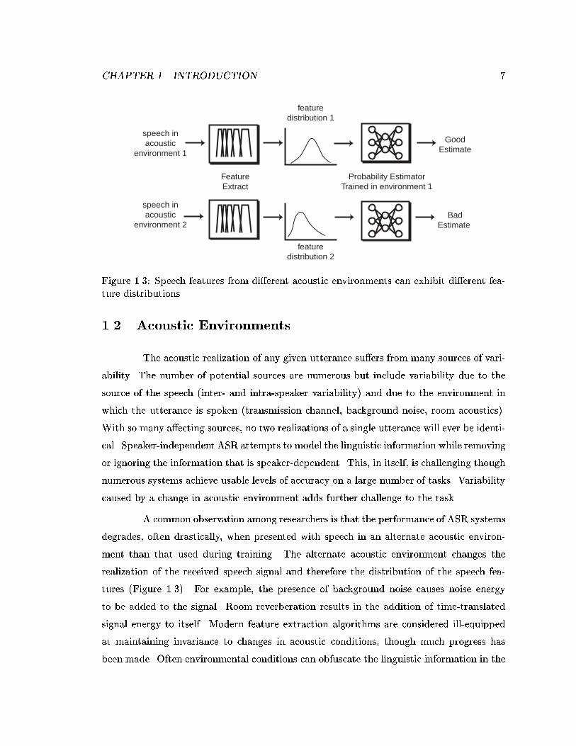
Figure 1.3: Speech features from di�erent acoustic environments can exhibit di�erent fea-ture distributions.
1.2 Acoustic Environments
The acoustic realization of any given utterance su�ers from many sources of vari-
ability. The number of potential sources are numerous but include variability due to the
source of the speech (inter- and intra-speaker variability) and due to the environment in
which the utterance is spoken (transmission channel, background noise, room acoustics).
With so many a�ecting sources, no two realizations of a single utterance will ever be identi-
cal. Speaker-independent ASR attempts to model the linguistic information while removing
or ignoring the information that is speaker-dependent. This, in itself, is challenging though
numerous systems achieve usable levels of accuracy on a large number of tasks. Variability
caused by a change in acoustic environment adds further challenge to the task.
A common observation among researchers is that the performance of ASR systems
degrades, often drastically, when presented with speech in an alternate acoustic environ-
ment than that used during training. The alternate acoustic environment changes the
realization of the received speech signal and therefore the distribution of the speech fea-
tures (Figure 1.3). For example, the presence of background noise causes noise energy
to be added to the signal. Room reverberation results in the addition of time-translated
signal energy to itself. Modern feature extraction algorithms are considered ill-equipped
at maintaining invariance to changes in acoustic conditions, though much progress has
been made. Often environmental conditions can obfuscate the linguistic information in the
CHAPTER 1. INTRODUCTION 8
Preprocessing
Linear Discriminant Analysis Components
DiscrimiativelyTrained
MLP
Temporal Processing Frequency-related processing
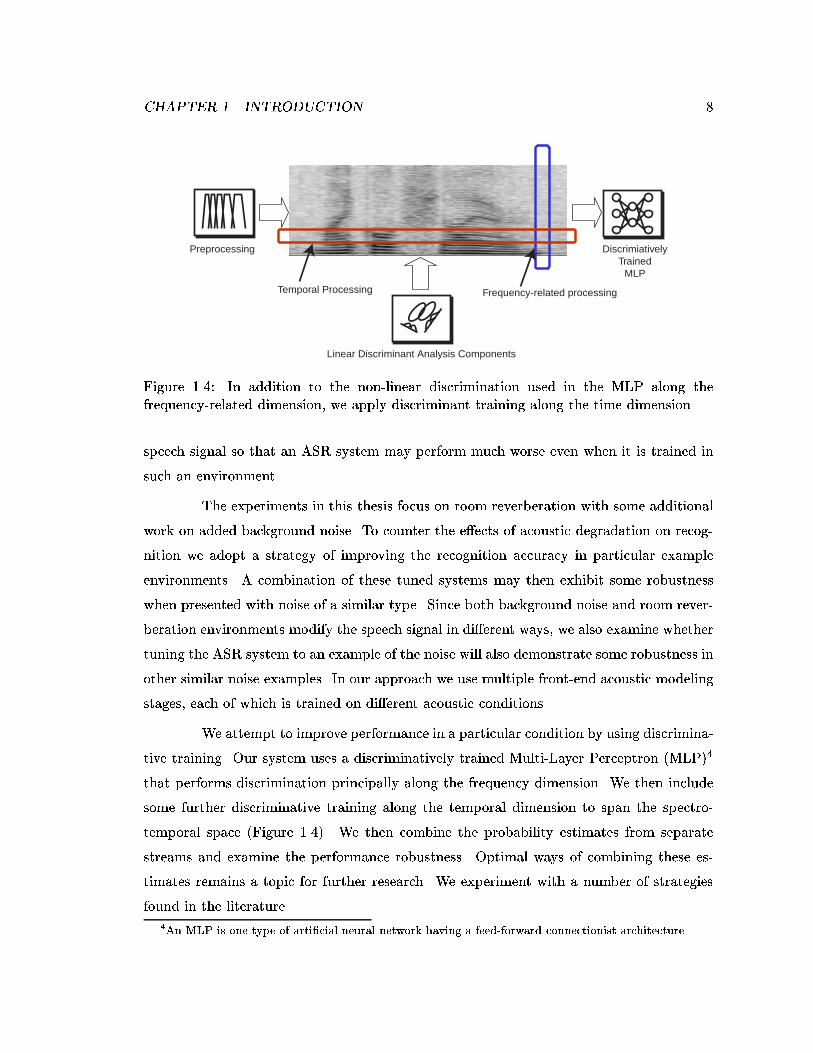
Figure 1.4: In addition to the non-linear discrimination used in the MLP along thefrequency-related dimension, we apply discriminant training along the time dimension.
speech signal so that an ASR system may perform much worse even when it is trained in
such an environment.
The experiments in this thesis focus on room reverberation with some additional
work on added background noise. To counter the e�ects of acoustic degradation on recog-
nition we adopt a strategy of improving the recognition accuracy in particular example
environments. A combination of these tuned systems may then exhibit some robustness
when presented with noise of a similar type. Since both background noise and room rever-
beration environments modify the speech signal in di�erent ways, we also examine whether
tuning the ASR system to an example of the noise will also demonstrate some robustness in
other similar noise examples. In our approach we use multiple front-end acoustic modeling
stages, each of which is trained on di�erent acoustic conditions.
We attempt to improve performance in a particular condition by using discrimina-
tive training. Our system uses a discriminatively trained Multi-Layer Perceptron (MLP)4
that performs discrimination principally along the frequency dimension. We then include
some further discriminative training along the temporal dimension to span the spectro-
temporal space (Figure 1.4). We then combine the probability estimates from separate
streams and examine the performance robustness. Optimal ways of combining these es-
timates remains a topic for further research. We experiment with a number of strategies
found in the literature.
4An MLP is one type of arti�cial neural network having a feed-forward connectionist architecture.
CHAPTER 1. INTRODUCTION 9
1.3 Overview
The goal of this work is to demonstrate that robustness to unseen acoustic envi-
ronment data can be achieved using the multi-stream approach. Many have experimented
with the multi-stream paradigm in ASR and some have explicitly tested the robustness to
noise conditions. It is common practice by researchers to conduct tests where the system
was trained in a single acoustic condition (usually with clean data) and tested with noisy
data. We deviate from this practice by adopting a strategy of a multi-stream system where
the components are expressly designed for or trained in separate acoustic conditions. The
course of this work proceeds in two stages. The �rst stage attempts to improve the front-
end acoustic modeling portion of the ASR system for speci�c acoustic environments. This
is accomplished through discriminative training of both the temporal �ltering in the feature
extraction routines and the probability-estimation components. With an appropriate set
of front-end components the second stage tests the performance of their combination with
special attention paid to the results using alternate, unseen acoustic conditions. Some of
the results in this document have been reported in [102, 103, 104]5.
This thesis proceeds as follows. Background information on ASR is described in
Chapter 2 with special attention paid to the front-end components. The use of an arti-
�cial neural network as a discriminatively trained probability estimator is described, as
are typical signal-processing strategies used in feature extraction. Also included are de-
scriptions of complete feature-extraction algorithms and the acoustic environments used
in most of the experiments. Finally, a description of the experimental setup is included
with further notes on the ASR system used. Chapter 3 describes the process of deriv-
ing temporal �lters using Linear Discriminant Analysis. Observations and trends of how
the discriminant �lters vary with acoustic condition are demonstrated. Recognition ex-
periments using RASTA-PLP with these �lters in matched and mismatched training and
testing conditions are described. In Chapter 4, we discuss the additional use of LDA for
temporal processing using alternate feature-extraction strategies. PLP and MSG6 are used
as the base feature-extraction algorithms that are augmented with LDA basis functions.
Chapter 5 describes experiments using multiple front-end acoustic modeling stages. Front-
5Some reported experimental results are di�erent due to changes in the ASR system setup.6Modulation-�ltered Spectrogram, a recent preprocessing algorithm developed by Kingsbury and Green-
berg [62].

CHAPTER 1. INTRODUCTION 10
ends using the augmented feature-extraction routines from previous sections are combined
and tested in unseen acoustic conditions. The tests comprise di�erent combinations of fea-
ture extraction and probability estimation components, each of which is trained and tested
under separate acoustic conditions. A number of encouraging results using simple combi-
nation strategies are examined and �nal tests with novel reverberation room impulses are
described. The �nal chapter summarizes the informative trends that can be observed from
the experiments. It also suggests avenues of further study and the promise of future im-
provement using multiple front-end components in ASR. Several appendices are included
that contain information related to this work.
11
Chapter 2
Automatic Speech Recognition
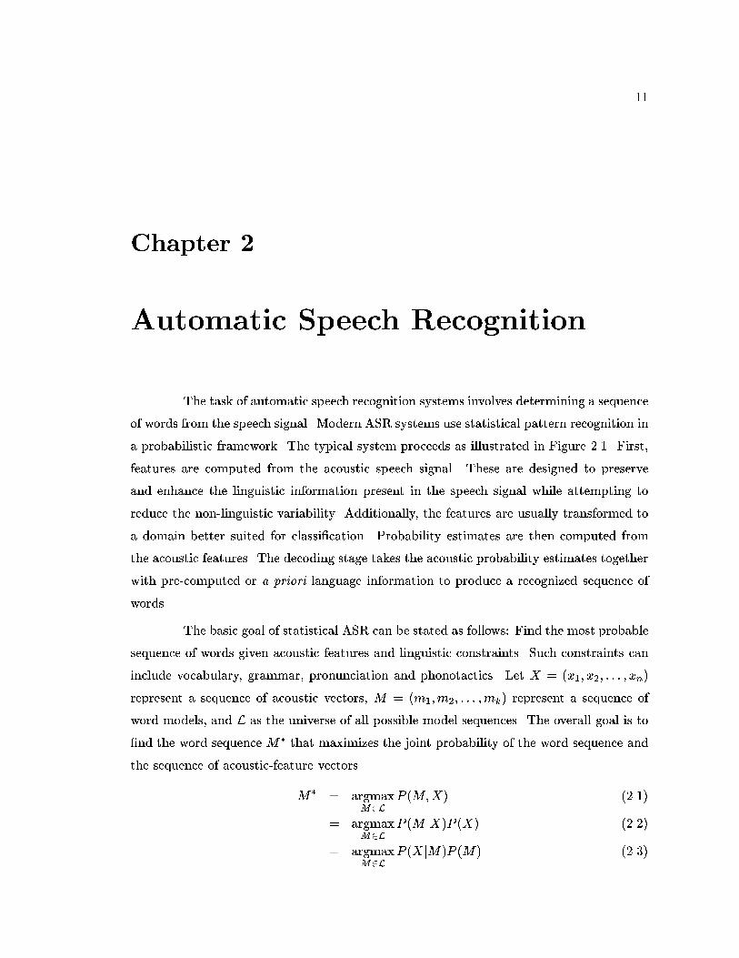
The task of automatic speech recognition systems involves determining a sequence
of words from the speech signal. Modern ASR systems use statistical pattern recognition in
a probabilistic framework. The typical system proceeds as illustrated in Figure 2.1. First,
features are computed from the acoustic speech signal. These are designed to preserve
and enhance the linguistic information present in the speech signal while attempting to
reduce the non-linguistic variability. Additionally, the features are usually transformed to
a domain better suited for classi�cation. Probability estimates are then computed from
the acoustic features. The decoding stage takes the acoustic probability estimates together
with pre-computed or a priori language information to produce a recognized sequence of
words.
The basic goal of statistical ASR can be stated as follows: Find the most probable
sequence of words given acoustic features and linguistic constraints. Such constraints can
include vocabulary, grammar, pronunciation and phonotactics. Let X = (x1; x2; : : : ; xn)
represent a sequence of acoustic vectors, M = (m1;m2; : : : ;mk) represent a sequence of
word models, and L as the universe of all possible model sequences. The overall goal is to
�nd the word sequence M� that maximizes the joint probability of the word sequence and
the sequence of acoustic-feature vectors.
M� = argmaxM2L
P (M;X) (2.1)
= argmaxM2L
P (M jX)P (X) (2.2)
= argmaxM2L
P (XjM)P (M) (2.3)
CHAPTER 2. AUTOMATIC SPEECH RECOGNITION 12
dog cat
a
the
0.1
0.3
0.2
0.1
FeatureExtraction
ProbabilityEstimate
Decode
Speech Words
PronunciationModels
GrammarModel
c a t
X M*
P(X|Q)or
P(Q|X)
P(M)
P(Q|M)
langΘ
acoustΘ
pronΘ
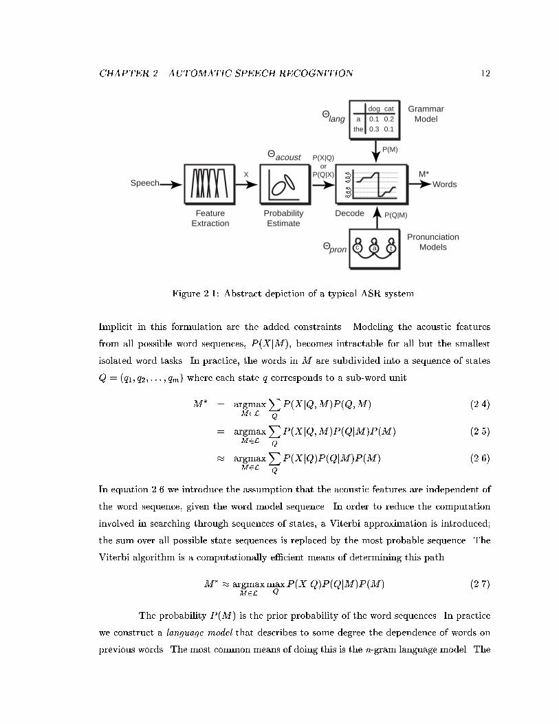
Figure 2.1: Abstract depiction of a typical ASR system.
Implicit in this formulation are the added constraints. Modeling the acoustic features
from all possible word sequences, P (XjM), becomes intractable for all but the smallest
isolated word tasks. In practice, the words in M are subdivided into a sequence of states
Q = (q1; q2; : : : ; qm) where each state q corresponds to a sub-word unit.
M� = argmaxM2L
XQ
P (XjQ;M)P (Q;M) (2.4)
= argmaxM2L
XQ
P (XjQ;M)P (QjM)P (M) (2.5)
� argmaxM2L
XQ
P (XjQ)P (QjM)P (M) (2.6)
In equation 2.6 we introduce the assumption that the acoustic features are independent of
the word sequence, given the word model sequence. In order to reduce the computation
involved in searching through sequences of states, a Viterbi approximation is introduced;
the sum over all possible state sequences is replaced by the most probable sequence. The
Viterbi algorithm is a computationally e�cient means of determining this path.
M� � argmaxM2L
maxQ
P (XjQ)P (QjM)P (M) (2.7)
The probability P (M) is the prior probability of the word sequences. In practice
we construct a language model that describes to some degree the dependence of words on
previous words. The most common means of doing this is the n-gram language model. The

CHAPTER 2. AUTOMATIC SPEECH RECOGNITION 13
P(q1|q1) P(q2|q2)
P(q2|q1)
P(x|q1) P(x|q2)
q1 q2
Figure 2.2: Hidden Markov Model.
probability of a given word in the sequence is dependent on only the previous n� 1 words.
P (M) = P (m1;m2; : : : ;mk) (2.8)
= P (m1)kYi=2
P (mijm1; : : : ;mi�1) (2.9)
= P (m1)P (m2jm1) : : :kY
i=n
P (mijmi�(n�1); : : : ;mi�1) (2.10)
The probability P (m1) is the unigram prior probability of the �rst word.
The probability P (QjM) is determined by using pronunciation models. Each word
is modeled by a stochastic �nite-state automaton as shown in Figure 2.2. Models include
a �rst-order Markov assumption.
P (qt+1jqt; qt�1; : : :) = P (qt+1jqt) (2.11)
A dictionary �le can be stored that contains all of the allowable words together with the
state sequences of each word and the associated transition probabilities. Often an interme-
diate collection of base-form sequences is introduced for convenience in large vocabulary
tasks.
P (QjM) = P (QjB)P (BjM) (2.12)
The B sequences often model complete phones including a distribution for phone duration
determined by the number of states and the transition probabilities. The word models can
be expressed as a concatenation of constituent phonemes. The phones usually are mod-
eled independently of the word sequence, though they need not be. Phones are, however,
CHAPTER 2. AUTOMATIC SPEECH RECOGNITION 14
sometimes modeled with a dependence on contextual phones. This is done to handle the
e�ects of variability due to coarticulation. This work uses context-independent phonemes
with states that correspond to phonetic classes. Many researchers have opted to subdi-
vide phone segments further (for example into tri-state phone models). Tri-state models
typically include states for the beginning, middle and ending of the phone.
The probability P (XjQ) is the acoustic likelihood probability. In the HMM frame-
work each acoustic feature xt is considered to be a random variable emitted from a single
state qt that is independent of other states and independent of other features given the
state.
P (XjQ) = P (x1; x2; : : : ; xN jQ) (2.13)
=NYt=1
P (xtjq1; q2; : : : ; qN ) (2.14)
=NYt=1
P (xtjqt) (2.15)
Equation 2.14 arises from the assumed conditional independence of the features given the
states. Equation 2.15 arises from the Markov assumption of the conditional independence
of states.
Complete ASR systems have many parameters that are trained to a given recog-
nition task. Some parameters are used for the acoustic probability estimation while others
are associated with the pronunciation models, language models and search. We treat these
parameters as separable and independently trainable.
M� � argmaxM2L
maxQ
P (XjQ;�acoust)P (QjM;�pron)P (M j�lang) (2.16)
�lang can include, for example, the unigram priors and the n-gram probabilities that are
estimated a priori from a speech corpus. �pron can include the state description and
transition probabilities for the sub-word models. These can also be estimated statically and
a priori from a speech corpus. There are also other system parameters that are manually
tuned. Some of these parameters are, for example, associated with the decoding stage, such
as adjusting the amount of search space that is pruned and the relative weighting of the
acoustic- and language-model scores. The experiments in this thesis concern the use of the
acoustic probabilities P (XjQ). These and their trained parameters, �acoust are discussed
CHAPTER 2. AUTOMATIC SPEECH RECOGNITION 15
further in the following section. The other components of the system are kept static and
not explored in this work.
2.1 Probability Estimation
The HMM emission probability distributions P (XjQ;�acoust) are most commonly
estimated from training data using Gaussian mixture models (GMMs) [87]. The distribu-
tion is characterized by a weighted sum of Gaussian density functions. The parameters
�acoust are the collection of means �k and covariances �k of the Gaussians and relative
weightings �k.
P (xjq) =Pk�k
(p2�j��1
kj)N e
�(x��k)��1
k(x��k)T (2.17)P
k �k = 1 (2.18)
where N is the number of components in feature vector x. The parameters are estimated
from a training data set using, for example, the Expectation-Maximization (EM) algorithm
[25].
An alternative method for acoustic probability estimation is used in hybrid Arti-
�cial Neural Network (ANN) - HMM systems. In these systems, discriminatively trained
ANNs directly estimate the acoustic posterior P (qjx) instead of the likelihood P (xjq). Asbefore, these quantities are related by Bayes rule, though the method of estimation is quite
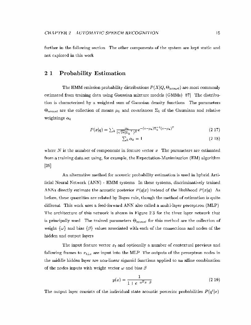
di�erent. This work uses a feed-forward ANN also called a multi-layer perceptron (MLP).
The architecture of this network is shown in Figure 2.3 for the three layer network that
is principally used. The trained parameters �acoust for this method are the collection of
weight f!g and bias f�g values associated with each of the connections and nodes of the
hidden and output layers.
The input feature vector xt and optionally a number of contextual previous and
following frames to xt�c are input into the MLP. The outputs of the perceptron nodes in
the middle hidden layer are non-linear sigmoid functions applied to an a�ne combination
of the nodes inputs with weight vector ! and bias �.
y(x) =1
1 + e�!T x+�(2.19)
The output layer consists of the individual state acoustic posterior probabilities P (qijx).
CHAPTER2.AUTOMATIC
SPEECHRECOGNITION
16
ωa
βω
bωc
context
output
inputcontext
hid
de
n
Figu
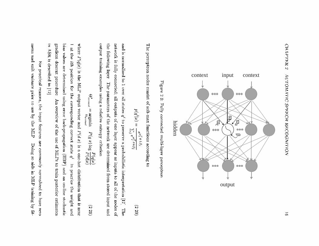
re2.3:
Fully
connected
multi-layer
percep
tron.
Thepercep
tronnodes
consist
ofsoft-m
axfunction
saccord
ingto
p(qijx
)=
e!Tix+�j
Pje!Tjx+�j
(2.20)
andisnorm
alizedto
1over
allstates
qito
preserve
aprob
abilistic
interp
retation[17
].The
netw
orkisfully
connected
;all
outputsof
onelayer
appear
asinputsto
allof
thenodes
of
thefollow
inglayer.
Theparam
etersof
thenetw
orkare
determ
ined
fromstored
inputand
outputtrain
ingexam
ples
usin
garelative
entrop
ycriterion
��acoust=argm
in�acoust
P(qjx
)log
P(qjx
)
P(djx
)(2.21)
where
P(qjx
)istheMLPoutputvector
andP(djx
)isaone-h
otdistrib
ution
that
isnear
1at
theith
position
forthecorresp
ondingcorrect
stateqi.
Inpractice
theweigh
tand
bias
values
aredeterm
ined
usin
gerror
back
-prop
agation(EBP)andan
on-lin
esto
chastic
gradien
tdescen
tproced
ure.
Anoverv
iewof
theuse
ofMLPsto
trainposterior
estimates
inASRisdescrib
edin
[12].
For
practical
reasons,theinputfeatu
resare
commonly
norm
alizedto
have
zero
mean
andunitvarian
ceprior
touse
bytheMLP.
Doin
gso
aidsin
MLPtrain
ingby�t-
CHAPTER 2. AUTOMATIC SPEECH RECOGNITION 17
ting the feature values to a known range coinciding with the \active" region of the sigmoid
function. This allows for selecting reasonable initial weights and has some numerical ad-
vantage. The input normalization parameters are computed over the training set, though
they can also be determined from each testing utterance or using an online estimate.
2.2 Speech Feature Extraction
A number of speech feature extraction algorithms exist; some are used for speaker
veri�cation as well as for speech recognition. Among the most common are Mel-Frequency
Cepstral Coe�cients (MFCC) [24] and RelAtive SpecTrAl - Perceptual Linear Prediction
(RASTA-PLP) [48, 50]. A number of variations exist but most contain common elements.
In particular, speech feature extraction involves a decomposition of the speech signal into
a time-frequency matrix to which further processing is applied. Such processing includes
frequency smoothing and temporal �ltering. Typically, transformations are applied to
aid in pattern recognition. Many of the processing steps applied to the time-frequency
matrix are inspired by human perception as well as by mathematical convenience. Other
processing steps are set though empirical experimentation or by experimenter intuition.
Some of the modi�cations have been designed to either reduce the e�ect of noise, model
a speci�c perceptual phenomenon or aid in probability estimation. This section brie y
describes some of the elements common to feature extraction routines that are used in
practice. In particular, elements of RASTA-PLP, which serves as a base extraction routine,
are described. Additionally, Modulation-�ltered Spectrogram (MSG), which is a relatively
recent algorithm developed at ICSI, is described [60, 62].
Analysis proceeds by �rst sampling the speech waveform with an analog-to-digital
conversion module. Since most of the speech information is carried in frequencies up to
3300 Hz and because the collection of utterances used for experimentation were recorded
over a band-limited telephone channel, the processing in this work assumes a sampling rate
of 8 kHz. The speech samples are stored for repeated analysis and all further processing is
carried out in the discrete domain.
CHAPTER 2. AUTOMATIC SPEECH RECOGNITION 18
2.2.1 Time-Frequency Analysis
Feature extraction techniques trace their origins to early synthesis and analysis
devices such as the Voder and Vocoder [29, 32]. Researchers noticed that phonetic segments
in speech appear as energy uctuations over time in di�erent frequency bands. This may be
observed by processing the speech signal through a bank of narrow-band �lters spanning
frequencies up to 4 kHz and examining the power present in each band over time. A
convenient alternative is to compute the magnitude squared of the Short-Term Fourier
Transform (STFT): The Discrete Fourier Transform (DFT) computed over a �nite window
of samples. The magnitude of the STFT is an estimate of the power spectral density,
under the assumption that the speech signal is locally stationary. This is not strictly
correct, though it is a common and useful assumption since speech can exhibit a quasi-
stationary behavior over a narrow segment of time. By computing the local power spectra
over adjacent windows of speech we obtain an estimate of the time evolution of the spectral
energy. The STFT is written as
X(m; k) =N�1Xn=0
x(pm+ n)w(n)e�j2�kn=N (2.22)
where w(n) is a �nite window frame that is \slid" over the speech waveform, N is the
length of the window, and p is the number of samples to step ahead. m represents the
current frame of speech and k represents the discrete frequency at frame m. A number of
di�erent window functions are used in practice. A common one that is used in this work
is the Hamming window:
w(n) =
8<: �� (1� �) cos( w�nN�1) : 0 � n � N � 1
0 : otherwise(2.23)
with � = 0:54. The windowing function reduces the e�ect of the discontinuity at the
endpoints since the DFT coe�cients assume a periodic signal. Multiplication in the discrete
time domain implies circular convolution in the discrete frequency domain. The window
therefore also smoothes the computed frequency values.
The magnitude square (jX(m; k)j2) completes the computation of the local powerspectral estimate. E�ectively, the phase information from the short-term spectral analysis,
which is largely considered unimportant for speech intelligibility, is discarded. Further,
since the speech signal is real, this quantity is symmetric and only half of the values
CHAPTER 2. AUTOMATIC SPEECH RECOGNITION 19
are kept for further analysis. Experiments reported in this work compute power spectral
estimates over 25-ms frames of speech stepped uniformly at 10-ms intervals.
Critical Bands
Frequency analysis in ASR often includes a number of approximations made from
observations by scientists studying auditory physiology and human auditory perception.
One such observation concerns the frequency resolution of the auditory periphery and, in
particular, the cochlea. The tonotopic organization of the cochlea itself suggests that the
human auditory system performs some kind of frequency analysis [38, 85]. Numerous per-
ceptual experiments have tested the detection of controlled signals, often in the presence of
masking noise. A commonly observed result pertains to the notion of the \critical-band"
�rst described by Fletcher in his masked sinusoid experiments [33, 2]. The phenomena in
general refers to the frequency-local processing and integration that occurs within the hu-
man auditory system. From numerous perceptual experiments, interference signals (such as
masking noise) outside of this critical bandwidth does not signi�cantly alter the detection
threshold of signals within the frequency range. This bandwidth is nonlinearly dependent
on frequency and sound pressure level. A number of functions approximating the frequency
dependence of the bandwidth were constructed as the result of speci�c experiments. For
example, the Bark scale, describes the frequency dependent bandwidth of a masking signal
over a sinusoidal signal [33, 124, 93]; the Mel scale approximates the frequency dependence
from experiments in pitch perception [106]; while a scale developed by Greenwood corre-
sponds to the frequency bandwidth for equal spacing along the cochlea [45]. The di�erent
experiments and scales have the commonality of being approximately logarithmic above
1 kHz. Below 1 kHz, the spacing is not logarithmic and sometimes modeled as nearly
linear. An alternative scaling with some of these properties is the constant-Q �lter-bank
with spacings ranging between one-third and one-fourth of an octave.
The critical-band scale is used in speech feature extraction for the spacing and
bandwidths of the �lter-bank. That is, �lters at higher frequencies have wider bandwidths
than at lower frequencies. RASTA-PLP, the primary base feature extraction method em-
ployed in this thesis, uses the Bark scale in its frequency analysis. The �lter-bank is
approximated by integrating discrete frequencies from an STFT along one-Bark intervals
with trapezoidal functions. The Bark intervals are determined from the following frequency
CHAPTER 2. AUTOMATIC SPEECH RECOGNITION 20
0 500 1000 1500 2000 2500 3000 3500 40000
0.2
0.4
0.6
0.8
1
Hz
Wei
ght
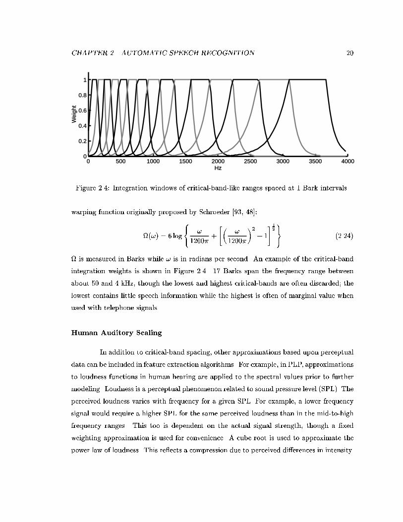
Figure 2.4: Integration windows of critical-band-like ranges spaced at 1 Bark intervals.
warping function originally proposed by Schroeder [93, 48]:
(!) = 6 log
8<: !
1200�+
"�!
1200�
�2+ 1
# 1
2
9=; (2.24)
is measured in Barks while ! is in radians per second. An example of the critical-band
integration weights is shown in Figure 2.4. 17 Barks span the frequency range between
about 50 and 4 kHz, though the lowest and highest critical-bands are often discarded; the
lowest contains little speech information while the highest is often of marginal value when
used with telephone signals.
Human Auditory Scaling
In addition to critical-band spacing, other approximations based upon perceptual
data can be included in feature extraction algorithms. For example, in PLP, approximations
to loudness functions in human hearing are applied to the spectral values prior to further
modeling. Loudness is a perceptual phenomenon related to sound pressure level (SPL). The
perceived loudness varies with frequency for a given SPL. For example, a lower frequency
signal would require a higher SPL for the same perceived loudness than in the mid-to-high
frequency ranges. This too is dependent on the actual signal strength, though a �xed
weighting approximation is used for convenience. A cube root is used to approximate the
power law of loudness. This re ects a compression due to perceived di�erences in intensity.
CHAPTER 2. AUTOMATIC SPEECH RECOGNITION 21
2.2.2 Feature Orthogonalization
Though spectral values convey much of the desired linguistic information they
are highly correlated. Adjacent frequency channels tend to rise and fall in synchrony and
therefore carry redundant information. In statistical pattern recognition tasks, it is often
helpful for modeling purposes to have feature components that are orthogonal. When using
Gaussian densities or mixtures of Gaussian densities, a considerable number of parameters
can be eliminated by using diagonal covariance matrices. Gaussian models can therefore
more accurately describe feature vectors with uncorrelated components.
Cepstra
The cepstrum (sometimes called the real cepstrum) is computed as the inverse
Fourier transform of the log magnitude of the Fourier transform of the signal portion of
interest.
c(m;n) =1
2�
N�1Xk=0
log jX(m; k)jej2�kn=N (2.25)
Here X(m; k) is the estimated power spectral values for the mth frame. Since the power
spectra are, by de�nition, real and symmetric this computation is equivalent to a Discrete
Cosine Transform. Restated, the log power spectral estimates are projected onto an or-
thogonal set of cosine basis functions. The o�-diagonal elements of the covariance matrix
of the coe�cients c(m;n) (computed over n) are very small, though they can be signi�cant
near the diagonal.
Cepstral processing is a subset of homomorphic processing techniques �rst studied
in depth by Bogert et. al.[9] and Oppenheim [84, 83]. A property of cepstral processing is
the separation of the signal into components that vary over time at di�erent rates. When
applied to speech along the time axis, it has demonstrated some utility in separating the
glottal source and vocal tract transfer function and has been used in pitch estimation [83].
In ASR, cepstra are commonly used for its quasi-orthogonalizing properties.
Linear Discriminant Analysis
Feature vectors can also be orthogonalized directly and completely over a given
data set, in contrast to the approximate decorrelation in cepstral processing. Two re-
CHAPTER 2. AUTOMATIC SPEECH RECOGNITION 22
lated methods used in statistics and pattern recognition are Principal Component Analysis
(PCA) and Linear Discriminant Analysis (LDA). LDA �gures prominently in this work,
though PCA is also described for comparison. In each, a set of orthonormal basis functions
�j that span the feature space are computed from statistics estimated from a training data
set. Further, these basis functions can be ranked by order of importance according to a
speci�c criterion. Let x represent the feature vector with D components and � a matrix
where each column is one of J basis vectors �j and J � D. The basis decomposition and
recombination can be written as:
yj = �Tj x (2.26)
y = �Tx (2.27)
x̂ = �y (2.28)
�T� = I (2.29)
Where y is a new feature vector, possibly of smaller dimension. PCA basis vectors are
obtained from minimizing the mean square error between the reconstructed and original
set of data vectors.
�PCA = argmin�
Xx
kx̂� xk2 (2.30)
= argmin�
Xx
k��Tx� xk2 (2.31)
It can be shown that the general solution satis�es the eigenvalue problem [35].
S�j = �j�j (2.32)
Where S = cov(x; x), the sample autocovariance matrix of x. The basis functions are
determined as the eigenvectors of the covariance matrix, �PCA = eig fSg. The new set of
basis functions amount to a rotation and alignment of the features according to dimensions
of maximum variance. This is also known as the discrete version of the Karhunen-Lo�eve
transform. The basis functions can be ranked in descending order of corresponding eigen-
values, corresponding to dimensions of decreasing amounts of variance. PCA guarantees
minimum reconstruction error when successive basis functions, corresponding to the small-
est eigenvalues, are eliminated. Interestingly, an informative result by Malayath [75] is that
the basis functions derived from PCA bear striking similarity to the cosine basis functions
from the DCT when applied to log spectral values. This result provides additional support
CHAPTER 2. AUTOMATIC SPEECH RECOGNITION 23
for using cepstra in pattern recognition tasks. The DCT has the added advantage of being
a simple and general decorrelation scheme, while the PCA basis vectors must be derived
from a given data set.
LDA basis functions are computed in a similar manner but through a di�erent
criterion.
�LDA = argmax�
j�TSB�jj�TSW�j (2.33)
The quantities SW and SB are the within-class and between-class covariances matrices
respectively. Taking X as a matrix, where each column corresponds to a feature vector,
and Xc as a matrix of feature vectors corresponding to class c 2 C, these quantities arecomputed as
SB =Xc2C
Nc(Xc �X)(Xc �X)T (2.34)
SW =Xc2C
(X �Xc)(X �Xc)T (2.35)
Xc =1
Nc
Xx2Xc
x (2.36)
X =1
N
Xx2X
x (2.37)
N is the number of example feature vectors and Nc is the number of example vectors
in class c. The basis functions that satisfy equation 2.33 are the solution to the general
eigenvalue problem [35].
SB�j = �jSW�j (2.38)
The basis functions are determined as the eigenvectors of the between-to-within covariance
ratio, �PCA = eignS�1W SB
o. The resulting rotation aligns the features to dimensions
of maximum linear separability among de�ned classes instead of among dimensions of
maximum variation. The LDA basis functions again can be ranked in order of principle
dimensions of linear separability according to the magnitude of the associated eigenvalues.
A related measure of class separability is the Fisher ratio [28, 76], which has several similar
de�nitions, but for our purposes is trace(S�1W SB). Intuitively, this is the ratio of the variance
between classes to the average variance within classes. Separability increases as the class
means are spread further apart and the spread of each class becomes more con�ned.
While PCA computes the principle dimensions of variability, it is not necessarily
optimally suited to tasks of class discrimination. Figure 2.5 is an illustrative example of
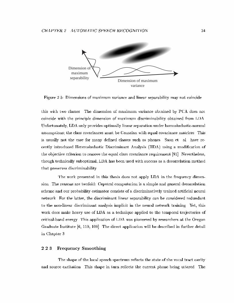
CHAPTER 2. AUTOMATIC SPEECH RECOGNITION 24
Dimension of maximumvariance
Dimension ofmaximum
separability
Figure 2.5: Dimensions of maximum variance and linear separability may not coincide.
this with two classes. The dimension of maximum variance obtained by PCA does not
coincide with the principle dimension of maximum discriminability obtained from LDA.
Unfortunately, LDA only provides optimally linear separation under homoskedastic-normal
assumptions; the class covariances must be Gaussian with equal covariance matrices. This
is usually not the case for many de�ned classes such as phones. Saon et. al. have re-
cently introduced Heteroskedastic Discriminant Analysis (HDA) using a modi�cation of
the objective criterion to remove the equal class covariance requirement [91]. Nevertheless,
though technically suboptimal, LDA has been used with success as a decorrelation method
that preserves discriminability.
The work presented in this thesis does not apply LDA in the frequency dimen-
sion. The reasons are twofold: Cepstral computation is a simple and general decorrelation
scheme and our probability estimator consists of a discriminatively trained arti�cial neural
network. For the latter, the discriminant linear separability can be considered redundant
to the non-linear discriminant analysis implicit in the neural network training. Yet, this
work does make heavy use of LDA as a technique applied to the temporal trajectories of
critical-band energy. This application of LDA was pioneered by researchers at the Oregon
Graduate Institute [6, 110, 109]. The direct application will be described in further detail
in Chapter 3.
2.2.3 Frequency Smoothing
The shape of the local speech spectrum re ects the state of the vocal tract cavity
and source excitation. This shape in turn re ects the current phone being uttered. The
CHAPTER 2. AUTOMATIC SPEECH RECOGNITION 25
pattern of resonances, known as formants, can be observed from the spectral envelope
and must usually be inferred from the �ne structure pattern of the harmonics. It can
be distorted by noise and the frequency characteristics of a microphone or transmission
channel. The formant patterns also vary with the speaker. Many techniques exist to
enhance and preserve the formant information. Common ones for ASR systems involve
types of frequency smoothing and are described here.
Dimensionality Reduction
One technique that has the added bene�t of reducing computation is dimensional-
ity reduction of orthogonalized feature vectors. As noted in the previous section, the linear
basis functions for each of the new features can be ranked in order of variability or class
separability. Truncating those feature coe�cients that correspond to the basis functions
that explain the least amount of variability removes a source of less useful variation in the
speech spectrum. These basis functions typically correspond to more rapidly changing �ne
structure in the speech spectrum. Eliminating these components e�ectively smoothes the
shape of the spectrum.
Similarly, smoothing can be done by truncating the number of cepstral coe�cients.
This can also be interpreted as a multiplication of the cepstra by a rectangular window.
After an inverse DCT, this is equivalent to convolution of the log speech spectrum by the
windows response. The rectangular window frequency response is well known to be a sinc
function which has a lowpass characteristic. In e�ect, the log spectrum is smoothed.
Linear Prediction
A more direct approach is linear prediction. Linear prediction has been used by
speech researchers since the 1960's as a tool for modeling the formant patterns directly
with an auto-regressive (AR) all-pole model
H(z) =1
1�Ppj=1 ajz
�j (2.39)
where p is the order of the model. The coe�cients aj are determined from minimizing
the error between the predicted model and the signal. This can be computed using algo-
rithms to solve the appropriate normal equations [74]. By using higher-order models, the
CHAPTER 2. AUTOMATIC SPEECH RECOGNITION 26
prediction error can be made arbitrarily small, though in this speci�c application it is not
desirable to model the spectrum with ultimate precision.
Intuitively, the model places poles (determined from the aj coe�cients) where the
peaks of the spectrum reside. This \peak-hugging" property is desirable as it emphasizes
the resonances of the vocal tract. It is often considered that these formant peaks are more
linguistically important than the spectral valleys. The AR model provides a good match
as it models the peaks more accurately than the valleys. Reducing the order of the model
reduces the number of poles for peak modeling and therefore results in a smoother function.
Restated, N values can be modeled exactly (to within a scaling factor) by an order p = N
AR model. By setting p < N , the model provides the best smoothed �t by pole placement,
in the mean-squared-error sense, between the autocorrelation functions.
2.2.4 Temporal Processing
In addition to frequency smoothing, pattern recognition has been aided by tem-
porally processing the sequence of spectral or spectrally related values. The most common
techniques include the use of delta features, Cepstral Mean Subtraction, and RASTA �l-
tering, each of which is brie y described here.
Delta Features
Delta cepstral features, introduced by Furui [36], provide a mechanism to capture
some of the dynamics of the speech in ASR. The cepstral features are appended with
an estimate of the �rst and sometimes second derivatives. The estimates are commonly
performed as a �nite di�erence, often of a smoothed time series
�c(m; k) = c(m; k) � c(m� 1; k) (2.40)
or as a regression,
�c(m; k) =
PTi=�T ric(m+ i; k)PT
i=�T r2i(2.41)
The second form is used primarily in this work.
ASR systems have consistently bene�ted from the addition of delta features
though it does increase the amount of computation required for probability estimation.
CHAPTER 2. AUTOMATIC SPEECH RECOGNITION 27
One of the e�ects of the delta computation is the removal of the DC component of the
cepstral trajectories. This is done directly in the Cepstral Mean Subtraction method.
Cepstral Mean Subtraction
In Cepstral Mean Subtraction (CMS), a time average of the cepstral values (the
DC value) is subtracted from the values at each frame.
cnew(m; k) = c(m; k) � c(k) (2.42)
c(k) =1
T
TXm=1
c(m; k) (2.43)
This is usually computed over the length T of a complete utterance as a way of normalizing
for channel e�ects and adjusting for spectral slope. Normalizing over the utterance length
introduces some latency in the processing, though it is a simple and e�ective technique.
Alternatively, online techniques such as highpass �ltering or normalization over a moving
window can also be applied instead. Related to CMS is RASTA �ltering.
RASTA Filtering
RASTA (RelAtive SpecTral Analysis) �ltering in general refers to �ltering of the
temporal trajectories of some function of each of the spectral values. The �lter is usually
applied to power spectra to which a compressive nonlinearity is applied, such as a root
power or logarithm. Typically the �ltering is done in the log-spectral domain as in CMS.
In contrast to CMS, the RASTA �lter is applied to the individual compressed spectral
bands instead of the linear combination of the compressed bands. Further, the RASTA
�lter is often a bandpass �lter rather than a strict mean removal �lter, as occurs in CMS.
The �ltering of individual bands allows for further operations such as additional frequency
smoothing and modeling.
The original RASTA �lter proposed by Hermansky and Morgan [50] is a �nite
di�erentiator followed by a leaky single-pole integrator.
H(z) =:25z2 + :125z1 � :125z�1 � :25z�2
1� �z�1(2.44)
The pole � = 0:94, determined from numerous recognition experiments, is commonly used.
The impulse and frequency response of this �lter are displayed in Figure 2.6. We refer to
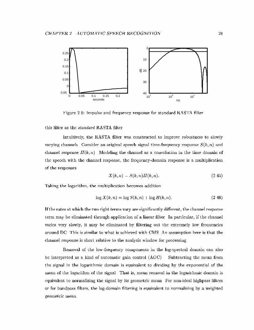
CHAPTER 2. AUTOMATIC SPEECH RECOGNITION 28
0 0.05 0.1 0.15 0.20.05
0
0.05
0.1
0.15
0.2
0.25
seconds10
110
010
140
30
20
10
0
Hz
dB
Figure 2.6: Impulse and frequency response for standard RASTA �lter.
this �lter as the standard RASTA �lter.
Intuitively, the RASTA �lter was constructed to improve robustness to slowly
varying channels. Consider an original speech signal time-frequency response S(k; n) and
channel response H(k; n). Modeling the channel as a convolution in the time domain of
the speech with the channel response, the frequency-domain response is a multiplication
of the responses
X(k; n) = S(k; n)H(k; n): (2.45)
Taking the logarithm, the multiplication becomes addition
logX(k; n) = log S(k; n) + logH(k; n): (2.46)
If the rates at which the two right terms vary are signi�cantly di�erent, the channel response
term may be eliminated through application of a linear �lter. In particular, if the channel
varies very slowly, it may be eliminated by �ltering out the extremely low frequencies
around DC. This is similar to what is achieved with CMS. An assumption here is that the
channel response is short relative to the analysis window for processing.
Removal of the low-frequency components in the log-spectral domain can also
be interpreted as a kind of automatic gain control (AGC). Subtracting the mean from
the signal in the logarithmic domain is equivalent to dividing by the exponential of the
mean of the logarithm of the signal. That is, mean removal in the logarithmic domain is
equivalent to normalizing the signal by its geometric mean. For non-ideal highpass �lters
or for bandpass �lters, the log-domain �ltering is equivalent to normalizing by a weighted
geometric mean.
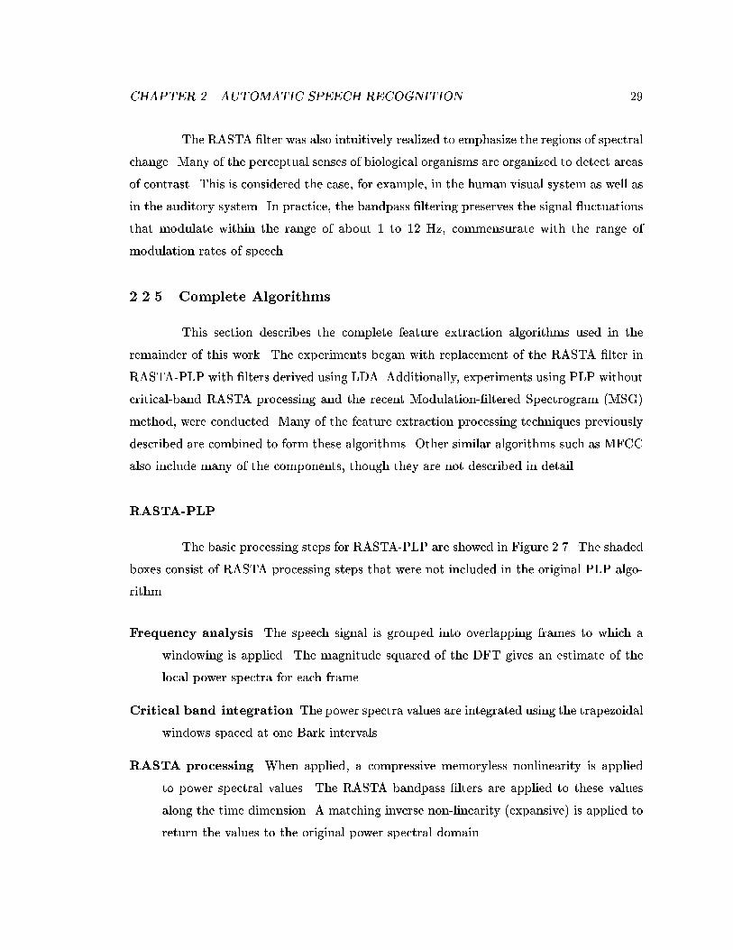
CHAPTER 2. AUTOMATIC SPEECH RECOGNITION 29
The RASTA �lter was also intuitively realized to emphasize the regions of spectral
change. Many of the perceptual senses of biological organisms are organized to detect areas
of contrast. This is considered the case, for example, in the human visual system as well as
in the auditory system. In practice, the bandpass �ltering preserves the signal uctuations
that modulate within the range of about 1 to 12 Hz, commensurate with the range of
modulation rates of speech.
2.2.5 Complete Algorithms
This section describes the complete feature extraction algorithms used in the
remainder of this work. The experiments began with replacement of the RASTA �lter in
RASTA-PLP with �lters derived using LDA. Additionally, experiments using PLP without
critical-band RASTA processing and the recent Modulation-�ltered Spectrogram (MSG)
method, were conducted. Many of the feature extraction processing techniques previously
described are combined to form these algorithms. Other similar algorithms such as MFCC
also include many of the components, though they are not described in detail.
RASTA-PLP
The basic processing steps for RASTA-PLP are showed in Figure 2.7. The shaded
boxes consist of RASTA processing steps that were not included in the original PLP algo-
rithm.
Frequency analysis. The speech signal is grouped into overlapping frames to which a
windowing is applied. The magnitude squared of the DFT gives an estimate of the
local power spectra for each frame.
Critical band integration The power spectra values are integrated using the trapezoidal
windows spaced at one Bark intervals.
RASTA processing. When applied, a compressive memoryless nonlinearity is applied
to power spectral values. The RASTA bandpass �lters are applied to these values
along the time dimension. A matching inverse non-linearity (expansive) is applied to
return the values to the original power spectral domain.
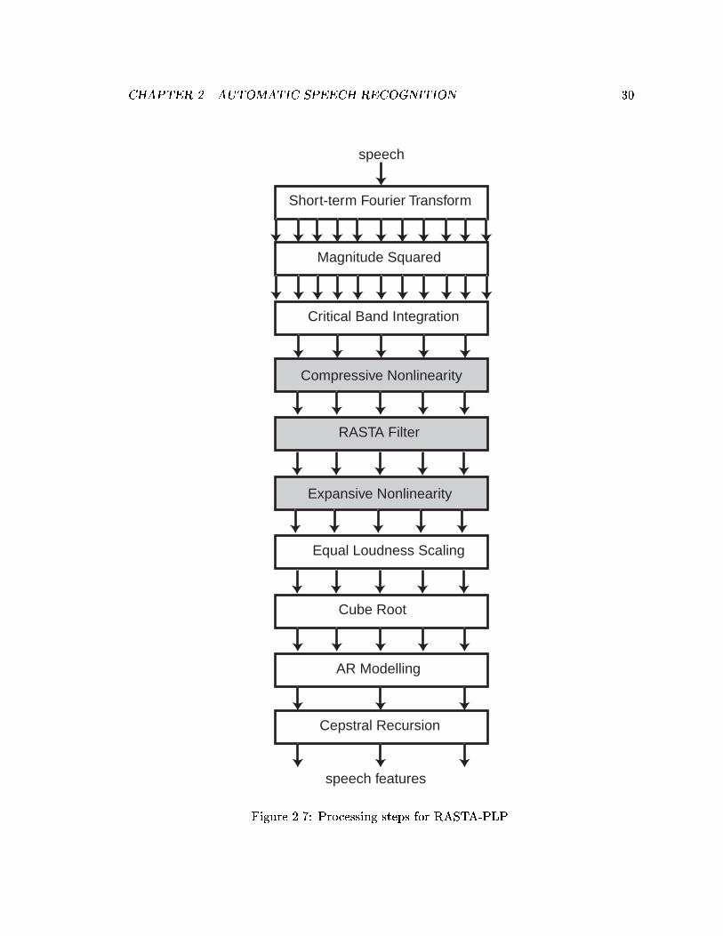
CHAPTER 2. AUTOMATIC SPEECH RECOGNITION 30
Magnitude Squared
Critical Band Integration
Compressive Nonlinearity
RASTA Filter
Expansive Nonlinearity
Equal Loudness Scaling
Short-term Fourier Transform
Cube Root
AR Modelling
Cepstral Recursion
speech
speech features
Figure 2.7: Processing steps for RASTA-PLP.
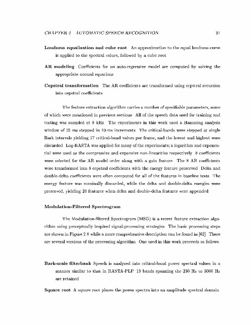
CHAPTER 2. AUTOMATIC SPEECH RECOGNITION 31
Loudness equalization and cube root. An approximation to the equal loudness curve
is applied to the spectral values, followed by a cube root.
AR modeling. Coe�cients for an auto-regressive model are computed by solving the
appropriate normal equations.
Cepstral transformation. The AR coe�cients are transformed using cepstral recursion
into cepstral coe�cients.
The feature extraction algorithm carries a number of speci�able parameters, some
of which were mentioned in previous sections. All of the speech data used for training and
testing was sampled at 8 kHz. The experiments in this work used a Hamming analysis
window of 25 ms stepped in 10-ms increments. The critical-bands were stepped at single
Bark intervals yielding 17 critical-band values per frame, and the lowest and highest were
discarded. Log-RASTA was applied for many of the experiments; a logarithm and exponen-
tial were used as the compressive and expansive non-linearities respectively. 8 coe�cients
were selected for the AR model order along with a gain feature. The 8 AR coe�cients
were transformed into 8 cepstral coe�cients with the energy feature preserved. Delta and
double-delta coe�cients were often computed for all of the features in baseline tests. The
energy feature was nominally discarded, while the delta and double-delta energies were
preserved, yielding 26 features when delta and double-delta features were appended.
Modulation-Filtered Spectrogram
The Modulation-�ltered Spectrogram (MSG) is a recent feature extraction algo-
rithm using perceptually inspired signal-processing strategies. The basic processing steps
are shown in Figure 2.8 while a more comprehensive description can be found in [62]. There
are several versions of the processing algorithm. One used in this work proceeds as follows.
Bark-scale �lterbank Speech is analyzed into critical-band power spectral values in a
manner similar to that in RASTA-PLP. 13 bands spanning the 230 Hz to 3000 Hz
are retained.
Square root A square root places the power spectra into an amplitude spectral domain.
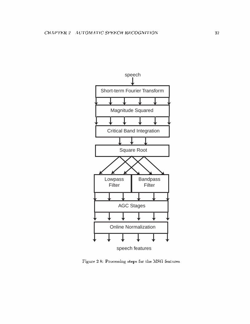
CHAPTER 2. AUTOMATIC SPEECH RECOGNITION 32
Magnitude Squared
Critical Band Integration
Short-term Fourier Transform
speech
speech features
LowpassFilter
BandpassFilter
Square Root
AGC Stages
Online Normalization
Figure 2.8: Processing steps for the MSG features.
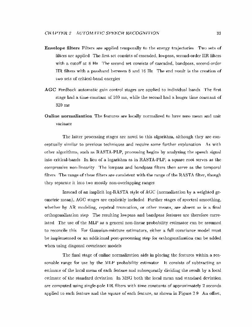
CHAPTER 2. AUTOMATIC SPEECH RECOGNITION 33
Envelope �lters Filters are applied temporally to the energy trajectories. Two sets of
�lters are applied. The �rst set consists of cascaded, lowpass, second-order IIR �lters
with a cuto� at 8 Hz. The second set consists of cascaded, bandpass, second-order
IIR �lters with a passband between 8 and 16 Hz. The end result is the creation of
two sets of critical-band energies.
AGC Feedback automatic gain control stages are applied to individual bands. The �rst
stage had a time constant of 160 ms, while the second had a longer time constant of
320 ms.
Online normalization The features are locally normalized to have zero mean and unit
variance.
The latter processing stages are novel to this algorithm, although they are con-
ceptually similar to previous techniques and require some further explanation. As with
other algorithms, such as RASTA-PLP, processing begins by analyzing the speech signal
into critical-bands. In lieu of a logarithm as in RASTA-PLP, a square root serves as the
compressive non-linearity. The lowpass and bandpass �lters then serve as the temporal
�lters. The range of these �lters are consistent with the range of the RASTA �lter, though
they separate it into two mostly non-overlapping ranges.
Instead of an implicit log-RASTA style of AGC (normalization by a weighted ge-
ometric mean), AGC stages are explicitly included. Further stages of spectral smoothing,
whether by AR modeling, cepstral truncation, or other means, are absent as is a �nal
orthogonalization step. The resulting lowpass and bandpass features are therefore corre-
lated. The use of the MLP as a general non-linear probability estimator can be assumed
to reconcile this. For Gaussian-mixture estimators, either a full covariance model must
be implemented or an additional post-processing step for orthogonalization can be added
when using diagonal covariance models.
The �nal stage of online normalization aids in placing the features within a rea-
sonable range for use by the MLP probability estimator. It consists of subtracting an
estimate of the local mean of each feature and subsequently dividing the result by a local
estimate of the standard deviation. In MSG both the local mean and standard deviation
are computed using single-pole IIR �lters with time constants of approximately 2 seconds
applied to each feature and the square of each feature, as shown in Figure 2.9. An o�set,
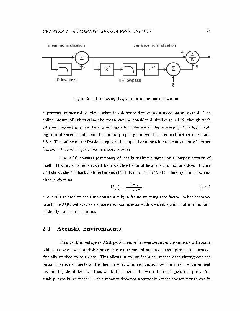
CHAPTER 2. AUTOMATIC SPEECH RECOGNITION 34
A
B
AB
-
+
X2 1/2
X Σ
Σ
ε
mean normalization variance normalization
IIR lowpassIIR lowpass
Figure 2.9: Processing diagram for online normalization.
", prevents numerical problems when the standard deviation estimate becomes small. The
online nature of subtracting the mean can be considered similar to CMS, though with
di�erent properties since there is no logarithm inherent in the processing. The local scal-
ing to unit variance adds another useful property and will be discussed further in Section
3.3.2. The online normalization stage can be applied or approximated conveniently in other
feature extraction algorithms as a post process.
The AGC consists principally of locally scaling a signal by a lowpass version of
itself. That is, a value is scaled by a weighted sum of locally surrounding values. Figure
2.10 shows the feedback architecture used in this rendition of MSG. The single pole lowpass
�lter is given as
H(z) =1� a
1� az�1(2.47)
where a is related to the time constant � by a frame stepping-rate factor. When incorpo-
rated, the AGC behaves as a square-root compressor with a variable gain that is a function
of the dynamics of the input.
2.3 Acoustic Environments
This work investigates ASR performance in reverberant environments with some
additional work with additive noise. For experimental purposes, examples of each are ar-
ti�cially applied to test data. This allows us to use identical speech data throughout the
recognition experiments and judge the e�ects on recognition by the speech environment
discounting the di�erences that would be inherent between di�erent speech corpora. Ar-
guably, modifying speech in this manner does not accurately re ect spoken utterances in
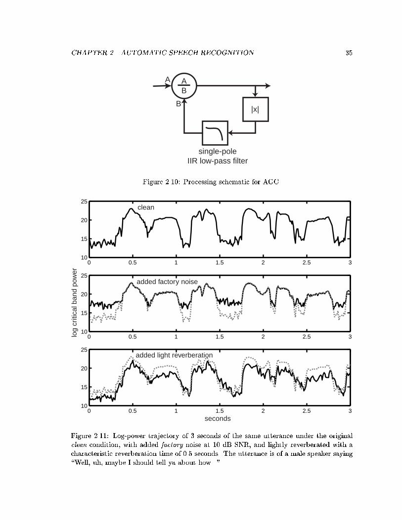
CHAPTER 2. AUTOMATIC SPEECH RECOGNITION 35
|x|
AB
A
B
single-poleIIR low-pass filter
Figure 2.10: Processing schematic for AGC.
0 0.5 1 1.5 2 2.5 310
15
20
25
0 0.5 1 1.5 2 2.5 310
15
20
25
0 0.5 1 1.5 2 2.5 310
15
20
25
clean
added factory noise
added light reverberation
log
criti
cal b
and
pow
er
seconds
Figure 2.11: Log-power trajectory of 3 seconds of the same utterance under the originalclean condition, with added factory noise at 10 dB SNR, and lightly reverberated with acharacteristic reverberation time of 0.5 seconds. The utterance is of a male speaker saying\Well, uh, maybe I should tell ya about how..."
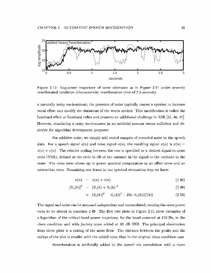
CHAPTER 2. AUTOMATIC SPEECH RECOGNITION 36
0 0.5 1 1.5 2 2.5 310
15
20
25added heavy reverberation
log
ampl
itude
seconds
Figure 2.12: Log-power trajectory of same utterance as in Figure 2.11 under severelyreverberated condition (characteristic reverberation time of 2.5 seconds).
a naturally noisy environment; the presence of noise typically causes a speaker to increase
vocal e�ort and modify the durations of the words spoken. This modi�cation is called the
Lombard e�ect or Lombard re ex and presents an additional challenge in ASR [57, 46, 47].
However, simulating a noisy environment in an arti�cial manner seems su�cient and de-
sirable for algorithm development purposes.
For additive noise, we simply add scaled samples of recorded noise to the speech
data. For a speech signal s(n) and noise signal v(n), the resulting signal x(n) is x(n) =
s(n) + v(n). The relative scaling between the two is speci�ed to a desired signal-to-noise
ratio (SNR), de�ned as the ratio in dB of the variance in the signal to the variance in the
noise. The noise term shows up in power spectral computation as an o�set term and an
interaction term. Examining one frame in our spectral estimation step we have:
x(n) = s(n) + v(n) (2.48)
jSx(k)j2 = jSs(k) + Sv(k)j2 (2.49)
= jSs(k)j2 + jSv(k)j2 + 2RejSs(k)S�v (k)j (2.50)
The signal and noise can be assumed independent and uncorrelated, causing the cross power
term to be absent in equation 2.49. The �rst two plots in Figure 2.11 show examples of
a logarithm of the critical-band power trajectory, for the band centered at 570 Hz, in the
clean condition and with factory noise added at 10 dB SNR. The principal observation
from these plots is a raising of the noise oor. The distance between the peaks and the
valleys of the plot is smaller with the added noise than in the original clean condition case.
Reverberation is arti�cially added to the speech via convolution with a room
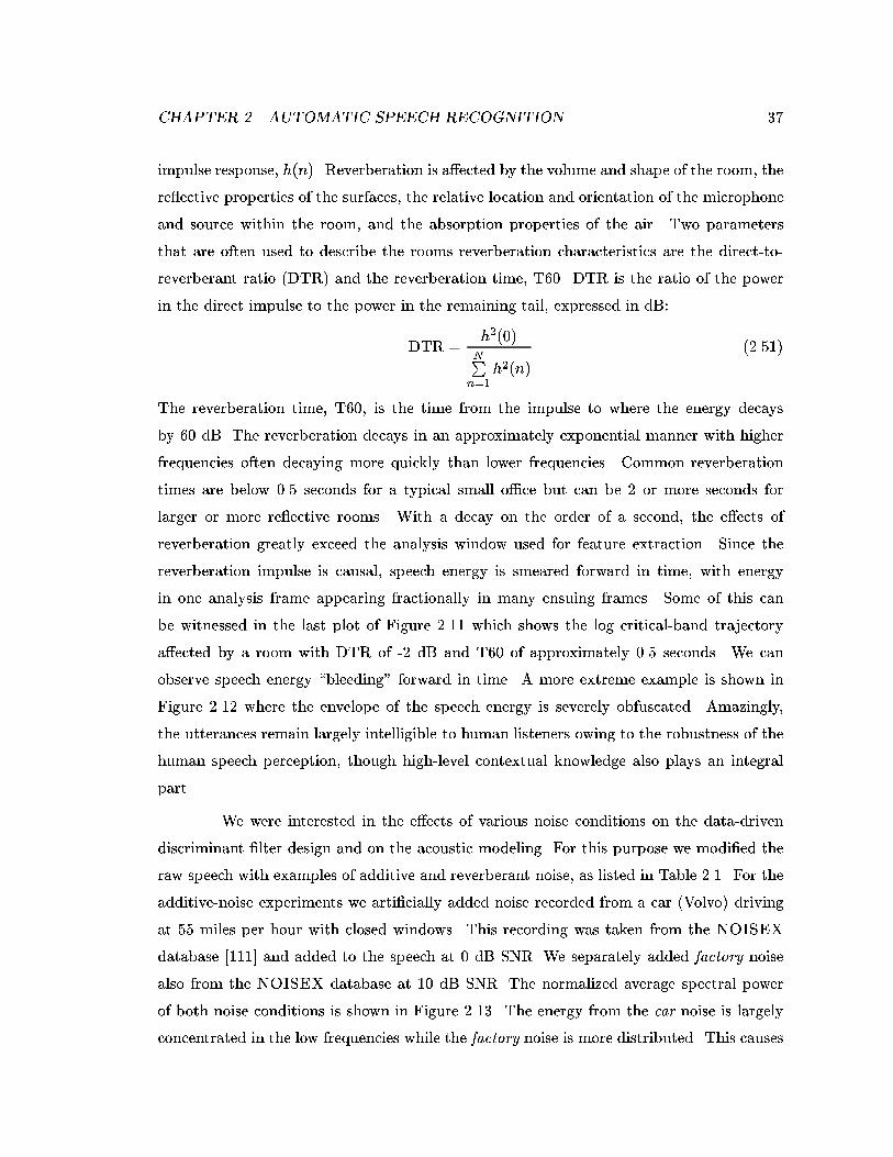
CHAPTER 2. AUTOMATIC SPEECH RECOGNITION 37
impulse response, h(n). Reverberation is a�ected by the volume and shape of the room, the
re ective properties of the surfaces, the relative location and orientation of the microphone
and source within the room, and the absorption properties of the air. Two parameters
that are often used to describe the rooms reverberation characteristics are the direct-to-
reverberant ratio (DTR) and the reverberation time, T60. DTR is the ratio of the power
in the direct impulse to the power in the remaining tail, expressed in dB:
DTR =h2(0)
NPn=1
h2(n)
(2.51)
The reverberation time, T60, is the time from the impulse to where the energy decays
by 60 dB. The reverberation decays in an approximately exponential manner with higher
frequencies often decaying more quickly than lower frequencies. Common reverberation
times are below 0.5 seconds for a typical small o�ce but can be 2 or more seconds for
larger or more re ective rooms. With a decay on the order of a second, the e�ects of
reverberation greatly exceed the analysis window used for feature extraction. Since the
reverberation impulse is causal, speech energy is smeared forward in time, with energy
in one analysis frame appearing fractionally in many ensuing frames. Some of this can
be witnessed in the last plot of Figure 2.11 which shows the log critical-band trajectory
a�ected by a room with DTR of -2 dB and T60 of approximately 0.5 seconds. We can
observe speech energy \bleeding" forward in time. A more extreme example is shown in
Figure 2.12 where the envelope of the speech energy is severely obfuscated. Amazingly,
the utterances remain largely intelligible to human listeners owing to the robustness of the
human speech perception, though high-level contextual knowledge also plays an integral
part.
We were interested in the e�ects of various noise conditions on the data-driven
discriminant �lter design and on the acoustic modeling. For this purpose we modi�ed the
raw speech with examples of additive and reverberant noise, as listed in Table 2.1. For the
additive-noise experiments we arti�cially added noise recorded from a car (Volvo) driving
at 55 miles per hour with closed windows. This recording was taken from the NOISEX
database [111] and added to the speech at 0 dB SNR. We separately added factory noise
also from the NOISEX database at 10 dB SNR. The normalized average spectral power
of both noise conditions is shown in Figure 2.13. The energy from the car noise is largely
concentrated in the low frequencies while the factory noise is more distributed. This causes
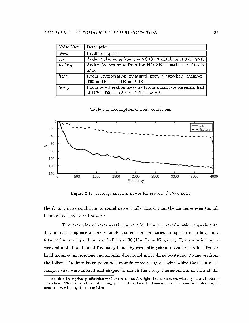
CHAPTER 2. AUTOMATIC SPEECH RECOGNITION 38
Noise Name Description
clean Unaltered speech
car Added Volvo noise from the NOISEX database at 0 dB SNR
factory Added factory noise from the NOISEX database at 10 dBSNR
light Room reverberation measured from a varechoic chamber.T60 = 0.5 sec, DTR = -2 dB
heavy Room reverberation measured from a concrete basement hallat ICSI. T60 = 2.5 sec, DTR = -8 dB
Table 2.1: Description of noise conditions.
0 500 1000 1500 2000 2500 3000 3500 4000140
120
100
80
60
40
20
0
Frequency
dB
car factory
Figure 2.13: Average spectral power for car and factory noise.
the factory noise conditions to sound perceptually noisier than the car noise even though
it possessed less overall power.1
Two examples of reverberation were added for the reverberation experiments.
The impulse response of one example was constructed based on speech recordings in a
6.1m � 2.4 m � 1.7 m basement hallway at ICSI by Brian Kingsbury. Reverberation times
were estimated in di�erent frequency bands by correlating simultaneous recordings from a
head-mounted microphone and an omni-directional microphone positioned 2.5 meters from
the talker. The impulse response was manufactured using decaying white Gaussian noise
samples that were �ltered and shaped to match the decay characteristics in each of the
1Another descriptive speci�cation would be to use an A weighted measurement, which applies a loudnesscorrection. This is useful for estimating perceived loudness by humans though it can be misleading inmachine-based recognition conditions.
CHAPTER 2. AUTOMATIC SPEECH RECOGNITION 39
frequency bands. Early re ections were added using estimates from a time-domain image
expansion simulation. The resulting impulse had a T60 of approximately 2.5 seconds and
a DTR ratio of -8 dB. This is referred to as the heavy or heavy reverberation condition in
this document. The impulse response of the other example was one of twelve recorded in
the Bell Labs Varechoic [113] chamber. This chamber is a 6.71 m � 5.94 m � 2.74 m room
composed of 368 panels that can be individually placed in an open or closed state. In the
closed state, the panel is highly re ective while in the open state highly absorbent material
is exposed. Measurements were recorded by four microphones placed 2 m, 2.35 m, 2.7 m,
and 3.05 m from the source with the room con�gured in three states: All panels closed,
43% of the panels open, and all panels open. The room impulses were estimated using a
chirp-excited system identi�cation method. The impulse used in most of the experiments
in this thesis was from the 2 m microphone with 43% of the panels open. It has a T60
of 0.5 seconds and a DTR of -2 dB and is referred to as the light or light reverberation
condition. The remaining room impulses were reserved for concluding tests.2
2.4 Experimental Setup
The research and experiments in this work were conducted at the International
Computer Science Institute (ICSI). The ASR system is a hybrid ANN-HMM system. Many
of the parameter choices for the recognition experiments, such as frame analysis windows,
stepping time, and number of feature coe�cients were described in previous sections. Only
the front-end components of the system were varied for these experiments; decoding algo-
rithms, speech corpora, and model parameters available in the ICSI research environment
were kept �xed during the experiments.
The ICSI system uses 56 mono-phone classes that are listed in Appendix A. HMM
states correspond to single phone classes. Most of the experiments listed here used the
Chronos speech decoder written by Tony Robinson at SoftSound, Cambridge, England
[89]. It is a stack-based decoder designed for large vocabulary tasks. Most of the manually
adjustable decoder parameters were kept at default values. However, the language model
scaling factor was set to yield the lowest word error rate on the small set of CV utterances.
The system uses context-independent phone models; phone models are independent of the
2Much appreciation goes to Brian Kingsbury and Carlos Avenda~no for providing me with these roomimpulse responses and measurements.
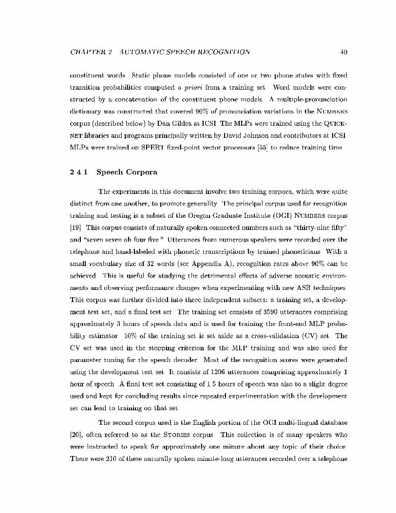
CHAPTER 2. AUTOMATIC SPEECH RECOGNITION 40
constituent words. Static phone models consisted of one or two phone states with �xed
transition probabilities computed a priori from a training set. Word models were con-
structed by a concatenation of the constituent phone models. A multiple-pronunciation
dictionary was constructed that covered 90% of pronunciation variations in the Numbers
corpus (described below) by Dan Gildea at ICSI. The MLPs were trained using the Quick-
net libraries and programs principally written by David Johnson and contributors at ICSI.
MLPs were trained on SPERT �xed-point vector processors [55] to reduce training time.
2.4.1 Speech Corpora
The experiments in this document involve two training corpora, which were quite
distinct from one another, to promote generality. The principal corpus used for recognition
training and testing is a subset of the Oregon Graduate Institute (OGI) Numbers corpus
[19]. This corpus consists of naturally spoken connected numbers such as \thirty-nine �fty"
and \seven seven oh four �ve." Utterances from numerous speakers were recorded over the
telephone and hand-labeled with phonetic transcriptions by trained phoneticians. With a
small vocabulary size of 32 words (see Appendix A), recognition rates above 90% can be
achieved. This is useful for studying the detrimental e�ects of adverse acoustic environ-
ments and observing performance changes when experimenting with new ASR techniques.
This corpus was further divided into three independent subsets: a training set, a develop-
ment test set, and a �nal test set. The training set consists of 3590 utterances comprising
approximately 3 hours of speech data and is used for training the front-end MLP proba-
bility estimator. 10% of the training set is set aside as a cross-validation (CV) set. The
CV set was used in the stopping criterion for the MLP training and was also used for
parameter tuning for the speech decoder. Most of the recognition scores were generated
using the development test set. It consists of 1206 utterances comprising approximately 1
hour of speech. A �nal test set consisting of 1.5 hours of speech was also to a slight degree
used and kept for concluding results since repeated experimentation with the development
set can lead to training on that set.
The second corpus used is the English portion of the OGI multi-lingual database
[20], often referred to as the Stories corpus. This collection is of many speakers who
were instructed to speak for approximately one minute about any topic of their choice.
There were 210 of these naturally spoken minute-long utterances recorded over a telephone
CHAPTER 2. AUTOMATIC SPEECH RECOGNITION 41
and hand-labeled and segmented into phonetic units by trained phoneticians. This corpus
is used solely as the data set for deriving discriminative temporal �lters. The procedure
involves analyzing relatively long time windows of speech. The length of the utterances
facilitated this longer temporal analysis; the utterances in the numbers corpus were on the
order of seconds in length instead of a minute. Further, the stories corpus has a much
larger vocabulary and a correspondingly larger number of phone examples. In contrast,
the Numbers corpus, with its limited vocabulary, contains examples for only 32 of the
56 possible phonetic classes listed in Appendix A. Finally, the independence of the two
corpora allows for testing the generality of the discriminatively trained �lters.
42
Chapter 3
LDA Temporal Filters for
RASTA-PLP
This chapter describes e�orts to improve word recognition in adverse acoustic
environments through discriminant training of the front-end acoustic modeling stages. In
our hybrid ANN-HMM system an MLP was discriminatively trained to classify phonetic
class targets. This MLP operated on features primarily along the frequency dimension. To
further improve classi�cation, discrimant training was added along the temporal dimen-
sion. Linear Discriminant Analysis was the tool that was used to derive discriminatively
trained temporal �lters. The experiments examined the �lter characteristics and word-
recognition performance in the presence of acoustic degradation using these temporal �lters
with RASTA-PLP preprocessing.
3.1 Temporal Filter Design with Linear Discriminant
Analysis
Linear Discriminant Analysis (LDA) has been used in speech feature extraction for
integrating adjacent feature frames, for feature selection and as an alternative to cepstral
analysis. Both LDA and cepstral techniques orthogonalize the feature-vector components
(the cepstra approximately so). LDA additionally arranges the feature components in di-
mensional order of linear separability. This procedure was often applied to one or more
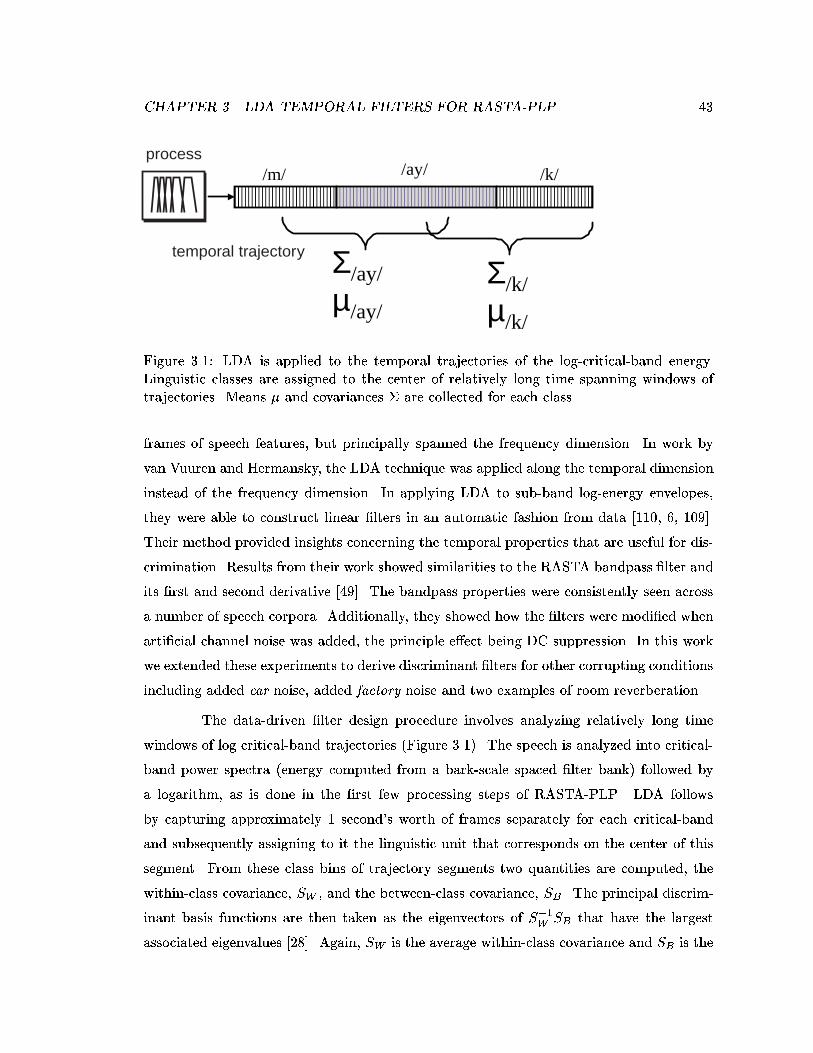
CHAPTER 3. LDA TEMPORAL FILTERS FOR RASTA-PLP 43
/m/ /ay/ /k/
Σ/ay/
µ/ay/
Σ/k/
µ/k/
process
temporal trajectory
Figure 3.1: LDA is applied to the temporal trajectories of the log-critical-band energy.Linguistic classes are assigned to the center of relatively long time spanning windows oftrajectories. Means � and covariances � are collected for each class.
frames of speech features, but principally spanned the frequency dimension. In work by
van Vuuren and Hermansky, the LDA technique was applied along the temporal dimension
instead of the frequency dimension. In applying LDA to sub-band log-energy envelopes,
they were able to construct linear �lters in an automatic fashion from data [110, 6, 109].
Their method provided insights concerning the temporal properties that are useful for dis-
crimination. Results from their work showed similarities to the RASTA bandpass �lter and
its �rst and second derivative [49]. The bandpass properties were consistently seen across
a number of speech corpora. Additionally, they showed how the �lters were modi�ed when
arti�cial channel noise was added, the principle e�ect being DC suppression. In this work
we extended these experiments to derive discriminant �lters for other corrupting conditions
including added car noise, added factory noise and two examples of room reverberation.
The data-driven �lter design procedure involves analyzing relatively long time
windows of log critical-band trajectories (Figure 3.1). The speech is analyzed into critical-
band power spectra (energy computed from a bark-scale spaced �lter bank) followed by
a logarithm, as is done in the �rst few processing steps of RASTA-PLP. LDA follows
by capturing approximately 1 second's worth of frames separately for each critical-band
and subsequently assigning to it the linguistic unit that corresponds on the center of this
segment. From these class bins of trajectory segments two quantities are computed, the
within-class covariance, SW , and the between-class covariance, SB . The principal discrim-
inant basis functions are then taken as the eigenvectors of S�1W SB that have the largest
associated eigenvalues [28]. Again, SW is the average within-class covariance and SB is the
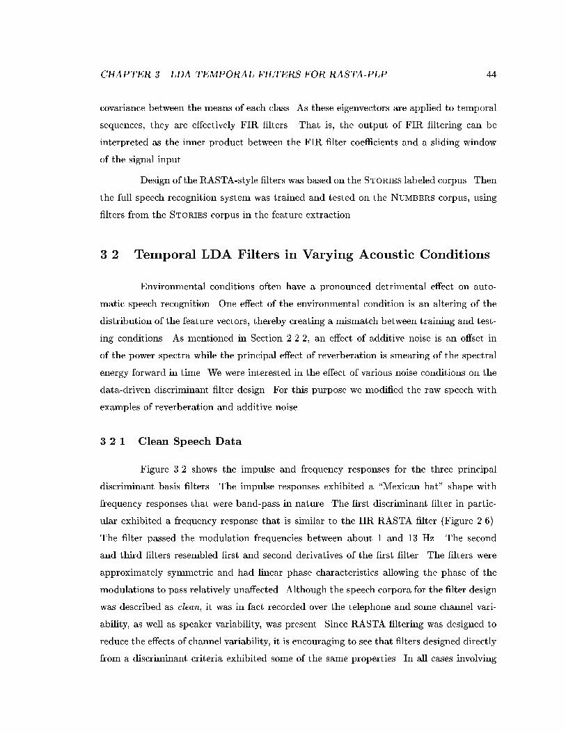
CHAPTER 3. LDA TEMPORAL FILTERS FOR RASTA-PLP 44
covariance between the means of each class. As these eigenvectors are applied to temporal
sequences, they are e�ectively FIR �lters. That is, the output of FIR �ltering can be
interpreted as the inner product between the FIR �lter coe�cients and a sliding window
of the signal input.
Design of the RASTA-style �lters was based on the Stories labeled corpus. Then
the full speech recognition system was trained and tested on the Numbers corpus, using
�lters from the Stories corpus in the feature extraction.
3.2 Temporal LDA Filters in Varying Acoustic Conditions
Environmental conditions often have a pronounced detrimental e�ect on auto-
matic speech recognition. One e�ect of the environmental condition is an altering of the
distribution of the feature vectors, thereby creating a mismatch between training and test-
ing conditions. As mentioned in Section 2.2.2, an e�ect of additive noise is an o�set in
of the power spectra while the principal e�ect of reverberation is smearing of the spectral
energy forward in time. We were interested in the e�ect of various noise conditions on the
data-driven discriminant �lter design. For this purpose we modi�ed the raw speech with
examples of reverberation and additive noise.
3.2.1 Clean Speech Data
Figure 3.2 shows the impulse and frequency responses for the three principal
discriminant basis �lters. The impulse responses exhibited a \Mexican hat" shape with
frequency responses that were band-pass in nature. The �rst discriminant �lter in partic-
ular exhibited a frequency response that is similar to the IIR RASTA �lter (Figure 2.6).
The �lter passed the modulation frequencies between about 1 and 13 Hz. The second
and third �lters resembled �rst and second derivatives of the �rst �lter. The �lters were
approximately symmetric and had linear phase characteristics allowing the phase of the
modulations to pass relatively una�ected. Although the speech corpora for the �lter design
was described as clean, it was in fact recorded over the telephone and some channel vari-
ability, as well as speaker variability, was present. Since RASTA �ltering was designed to
reduce the e�ects of channel variability, it is encouraging to see that �lters designed directly
from a discriminant criteria exhibited some of the same properties. In all cases involving
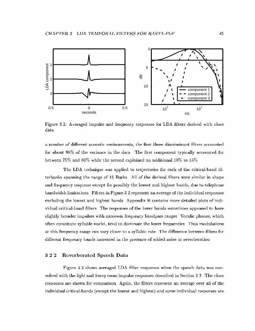
CHAPTER 3. LDA TEMPORAL FILTERS FOR RASTA-PLP 45
0.5 0 0.5
3
2
1
seconds
LDA
com
pone
nt
100
101
15
10
5
0
Hz
dB
component 1component 2component 3
Figure 3.2: Averaged impulse and frequency responses for LDA �lters derived with clean
data.
a number of di�erent acoustic environments, the �rst three discriminant �lters accounted
for about 95% of the variance in the data. The �rst component typically accounted for
between 75% and 80% while the second explained an additional 10% to 15%.
The LDA technique was applied to trajectories for each of the critical-band �l-
terbanks spanning the range of 15 Barks. All of the derived �lters were similar in shape
and frequency response except for possibly the lowest and highest bands, due to telephone
bandwidth limitations. Filters in Figure 3.2 represent an average of the individual responses
excluding the lowest and highest bands. Appendix B contains more detailed plots of indi-
vidual critical-band �lters. The responses of the lower bands sometimes appeared to have
slightly broader impulses with narrower frequency bandpass ranges. Vocalic phones, which
often constitute syllable nuclei, tend to dominate the lower frequencies. Thus modulations
at this frequency range can vary closer to a syllabic rate. The di�erence between �lters for
di�erent frequency bands increased in the presence of added noise or reverberation.
3.2.2 Reverberated Speech Data
Figure 3.3 shows averaged LDA �lter responses when the speech data was con-
volved with the light and heavy room impulse responses described in Section 2.3. The clean
responses are shown for comparison. Again, the �lters represent an average over all of the
individual critical-bands (except the lowest and highest) and some individual responses are
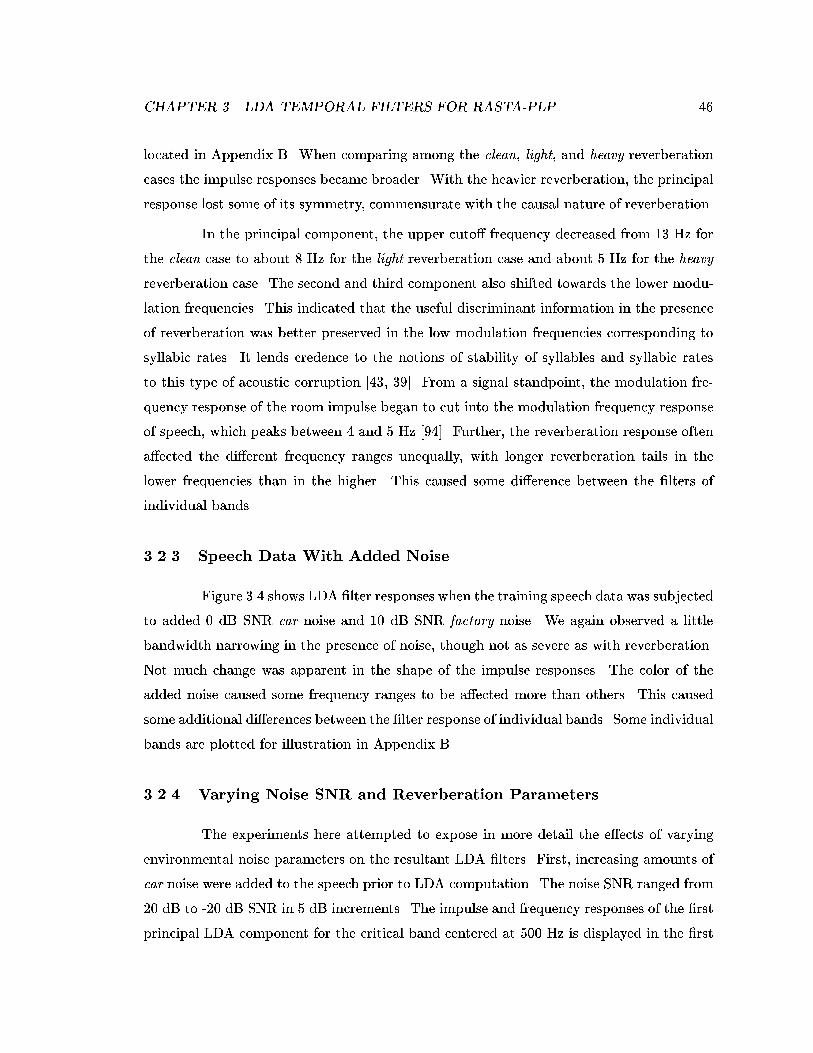
CHAPTER 3. LDA TEMPORAL FILTERS FOR RASTA-PLP 46
located in Appendix B. When comparing among the clean, light, and heavy reverberation
cases the impulse responses became broader. With the heavier reverberation, the principal
response lost some of its symmetry, commensurate with the causal nature of reverberation.
In the principal component, the upper cuto� frequency decreased from 13 Hz for
the clean case to about 8 Hz for the light reverberation case and about 5 Hz for the heavy
reverberation case. The second and third component also shifted towards the lower modu-
lation frequencies. This indicated that the useful discriminant information in the presence
of reverberation was better preserved in the low modulation frequencies corresponding to
syllabic rates. It lends credence to the notions of stability of syllables and syllabic rates
to this type of acoustic corruption [43, 39]. From a signal standpoint, the modulation fre-
quency response of the room impulse began to cut into the modulation frequency response
of speech, which peaks between 4 and 5 Hz [94]. Further, the reverberation response often
a�ected the di�erent frequency ranges unequally, with longer reverberation tails in the
lower frequencies than in the higher. This caused some di�erence between the �lters of
individual bands.
3.2.3 Speech Data With Added Noise
Figure 3.4 shows LDA �lter responses when the training speech data was subjected
to added 0 dB SNR car noise and 10 dB SNR factory noise. We again observed a little
bandwidth narrowing in the presence of noise, though not as severe as with reverberation.
Not much change was apparent in the shape of the impulse responses. The color of the
added noise caused some frequency ranges to be a�ected more than others. This caused
some additional di�erences between the �lter response of individual bands. Some individual
bands are plotted for illustration in Appendix B.
3.2.4 Varying Noise SNR and Reverberation Parameters
The experiments here attempted to expose in more detail the e�ects of varying
environmental noise parameters on the resultant LDA �lters. First, increasing amounts of
car noise were added to the speech prior to LDA computation. The noise SNR ranged from
20 dB to -20 dB SNR in 5 dB increments. The impulse and frequency responses of the �rst
principal LDA component for the critical band centered at 500 Hz is displayed in the �rst
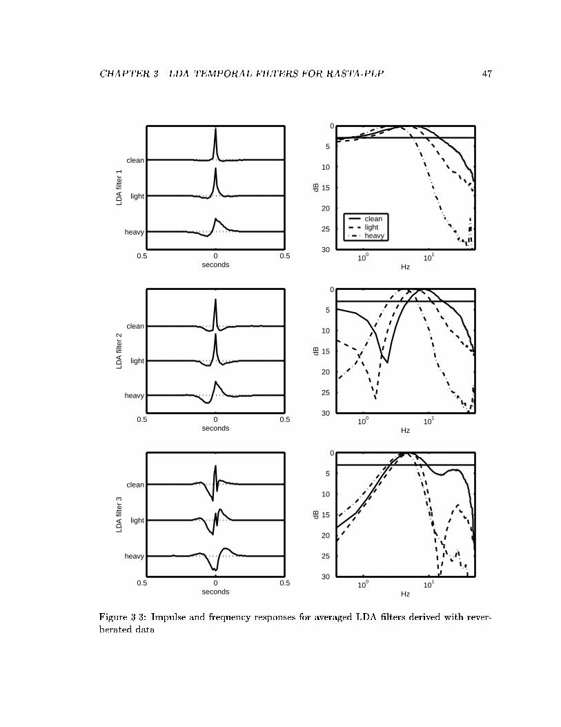
CHAPTER 3. LDA TEMPORAL FILTERS FOR RASTA-PLP 47
0.5 0 0.5
heavy
light
clean
seconds
LDA
filte
r 1
100
101
30
25
20
15
10
5
0
Hz
dB
cleanlightheavy
0.5 0 0.5
heavy
light
clean
seconds
LDA
filte
r 2
100
101
30
25
20
15
10
5
0
Hz
dB
0.5 0 0.5
heavy
light
clean
seconds
LDA
filte
r 3
100
101
30
25
20
15
10
5
0
Hz
dB
Figure 3.3: Impulse and frequency responses for averaged LDA �lters derived with rever-berated data.
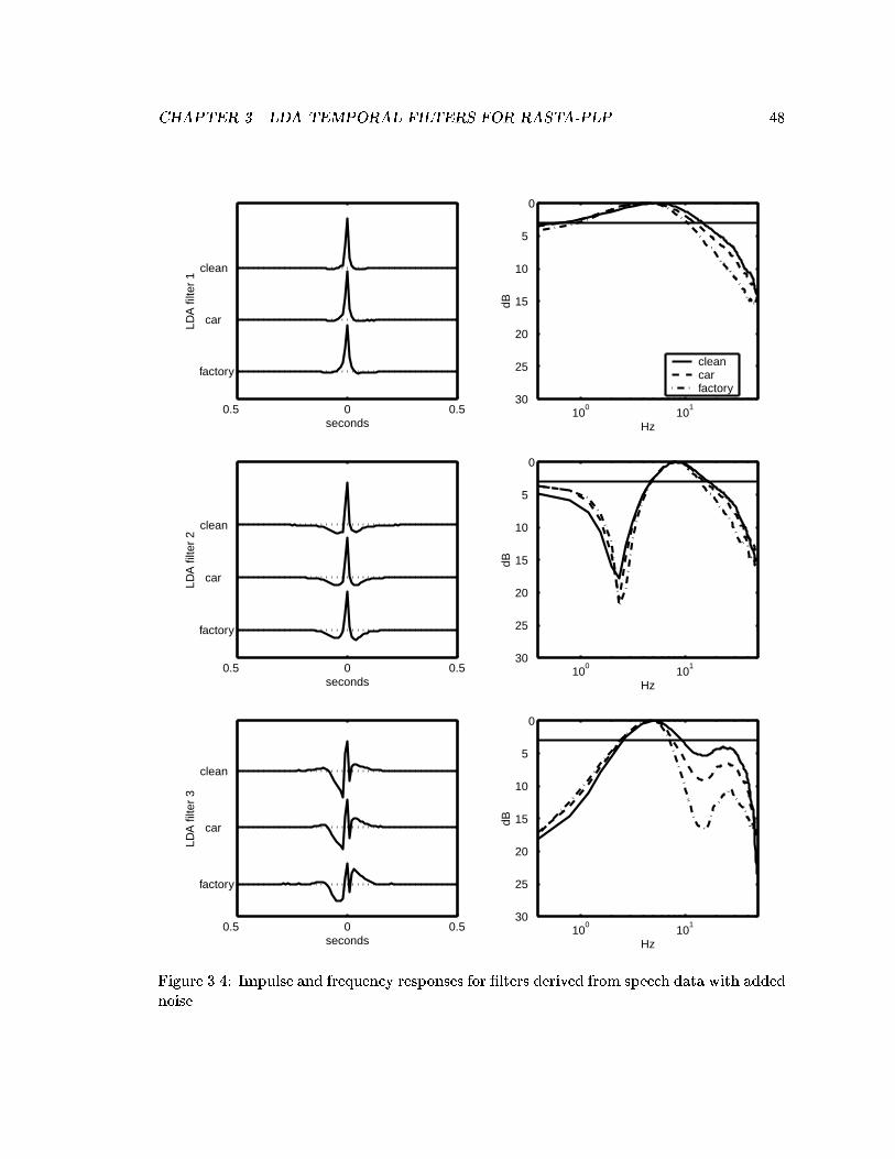
CHAPTER 3. LDA TEMPORAL FILTERS FOR RASTA-PLP 48
0.5 0 0.5
factory
car
clean
seconds
LDA
filte
r 1
100
101
30
25
20
15
10
5
0
Hz
dB
clean car factory
0.5 0 0.5
factory
car
clean
seconds
LDA
filte
r 2
100
101
30
25
20
15
10
5
0
Hz
dB
0.5 0 0.5
factory
car
clean
seconds
LDA
filte
r 3
100
101
30
25
20
15
10
5
0
Hz
dB
Figure 3.4: Impulse and frequency responses for �lters derived from speech data with addednoise.
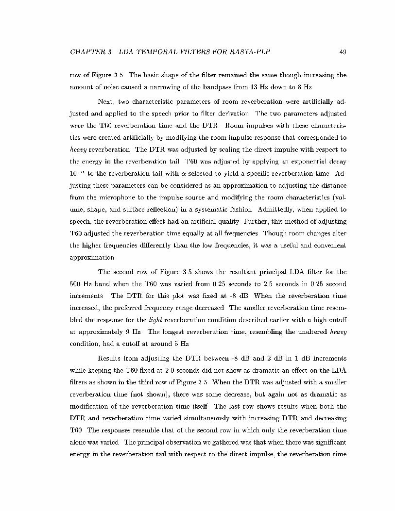
CHAPTER 3. LDA TEMPORAL FILTERS FOR RASTA-PLP 49
row of Figure 3.5. The basic shape of the �lter remained the same though increasing the
amount of noise caused a narrowing of the bandpass from 13 Hz down to 8 Hz.
Next, two characteristic parameters of room reverberation were arti�cially ad-
justed and applied to the speech prior to �lter derivation. The two parameters adjusted
were the T60 reverberation time and the DTR. Room impulses with these characteris-
tics were created arti�cially by modifying the room impulse response that corresponded to
heavy reverberation. The DTR was adjusted by scaling the direct impulse with respect to
the energy in the reverberation tail. T60 was adjusted by applying an exponential decay
10�� to the reverberation tail with � selected to yield a speci�c reverberation time. Ad-
justing these parameters can be considered as an approximation to adjusting the distance
from the microphone to the impulse source and modifying the room characteristics (vol-
ume, shape, and surface re ection) in a systematic fashion. Admittedly, when applied to
speech, the reverberation e�ect had an arti�cial quality. Further, this method of adjusting
T60 adjusted the reverberation time equally at all frequencies. Though room changes alter
the higher frequencies di�erently than the low frequencies, it was a useful and convenient
approximation.
The second row of Figure 3.5 shows the resultant principal LDA �lter for the
500 Hz band when the T60 was varied from 0.25 seconds to 2.5 seconds in 0.25 second
increments. The DTR for this plot was �xed at -8 dB. When the reverberation time
increased, the preferred frequency range decreased. The smaller reverberation time resem-
bled the response for the light reverberation condition described earlier with a high cuto�
at approximately 9 Hz. The longest reverberation time, resembling the unaltered heavy
condition, had a cuto� at around 5 Hz.
Results from adjusting the DTR between -8 dB and 2 dB in 1 dB increments
while keeping the T60 �xed at 2.0 seconds did not show as dramatic an e�ect on the LDA
�lters as shown in the third row of Figure 3.5. When the DTR was adjusted with a smaller
reverberation time (not shown), there was some decrease, but again not as dramatic as
modi�cation of the reverberation time itself. The last row shows results when both the
DTR and reverberation time varied simultaneously with increasing DTR and decreasing
T60. The responses resemble that of the second row in which only the reverberation time
alone was varied. The principal observation we gathered was that when there was signi�cant
energy in the reverberation tail with respect to the direct impulse, the reverberation time
CHAPTER 3. LDA TEMPORAL FILTERS FOR RASTA-PLP 50
0.5 0 0.50.5
0
0.5
1V
ary
SN
R
100 10130
25
20
15
10
5
0
dB
0.5 0 0.50.5
0
0.5
1
Var
y T
60
100 10130
25
20
15
10
5
0
dB
0.5 0 0.51
0.5
0
0.5
1
Var
y D
TR
100 10130
25
20
15
10
5
0
dB
0.5 0 0.50.5
0
0.5
1
Var
y D
TR
and
T60
seconds100 101
30
25
20
15
10
5
0
dB
Hz
DecreasingSNR
IncreasingT60
DecreasingDTR
IncreasingT60 andDecreasingDTR
Figure 3.5: Impulse and frequency responses for �lters derived with varying car noise SNR,reverberation T60, reverberation DTR, and reverberation T60 and DTR.
CHAPTER 3. LDA TEMPORAL FILTERS FOR RASTA-PLP 51
dominated the changes in the LDA �lter's preferred frequency range.
Experiments were also conducted where the �lters were derived using both clean
and heavy reverberation data together. Figure 3.6 shows LDA �lter responses when varying
the proportion of clean and heavy training data. The proportion ranged from equal parts
of each to purely heavy reverberation training data. With equal proportions, the �lter
resembled that of the pure clean case. This was because the covariances for the clean
conditions were larger than their heavily reverberated counterpart. One can recall for
example in Figure 2.12 that the \smearing" e�ect of the heavy reverberation leads to a
atter critical-band trajectory than the clean example. This atter trajectory leads to
a smaller variance range and the clean case would then dominate the LDA computation.
However, when the proportion of heavy reverberation data became signi�cant, the response
\morphed" smoothly between the two extremes. At some point in the transition the �lter
resembled that derived in the light reverberation case.
3.3 Recognition Results
This section reports recognition results using the LDA-derived �lters as a replace-
ment for the standard single-pole RASTA �lter (Figure 3.7). Since we were interested in
recognition performance in a variety of acoustic environments the tabulated results include
mismatched tests (i.e. tests using speech in conditions other than the one that the front-end
acoustic modeling was trained). In the tabulated scores the elements along the diagonal
correspond to matched training and testing conditions.
3.3.1 Initial Experiments
Tables 3.1 and 3.2 contain the frame accuracy and recognition results respectively
using the original RASTA �lter. Frame accuracy is determined by declaring a hard classi-
�cation on each frame based upon the maximum posterior estimate1. For each frame the
phone with the highest posterior probability estimate is declared as the recognized class
and is registered as a correct classi�cation if it corresponds to the reference phonetic tran-
scription. Word error rate (WER) consists of the ratio of the number of mis-recognized
1Classi�cation based upon maximum a posteriori probabilities is often referred to as Bayesianclassi�cation.
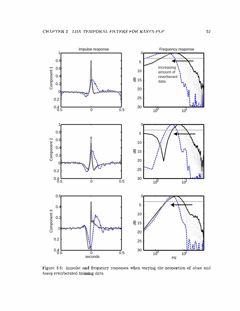
CHAPTER 3. LDA TEMPORAL FILTERS FOR RASTA-PLP 52
0.5 0 0.50.4
0.2
0
0.2
0.4
0.6
0.8
1C
ompo
nent
1Impulse response
100 10130
25
20
15
10
5
0
dB
Frequency response
0.5 0 0.50.4
0.2
0
0.2
0.4
0.6
0.8
1
Com
pone
nt 2
100 10130
25
20
15
10
5
0
dB
0.5 0 0.50.4
0.2
0
0.2
0.4
0.6
Com
pone
nt 3
seconds100 101
30
25
20
15
10
5
0
dB
Hz
Increasingamount ofreverberantdata
Figure 3.6: Impulse and frequency responses when varying the proportion of clean andheavy reverberated training data.
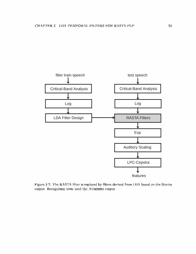
CHAPTER 3. LDA TEMPORAL FILTERS FOR RASTA-PLP 53
Critical-Band Analysis
Log
LDA Filter Design
Exp
Auditory Scaling
LPC-Cepstra
RASTA Filters
Critical-Band Analysis
Log
filter train speech test speech
features
Figure 3.7: The RASTA �lter is replaced by �lters derived from LDA based on the Storiescorpus. Recognition tests used the Numbers corpus.
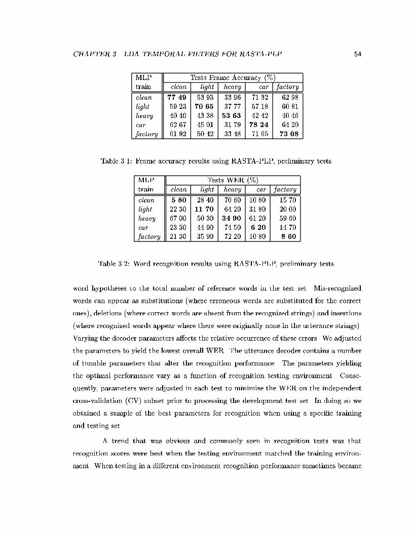
CHAPTER 3. LDA TEMPORAL FILTERS FOR RASTA-PLP 54
MLP Tests Frame Accuracy (%)train clean light heavy car factory
clean 77.49 53.93 33.96 71.32 62.98light 59.23 70.65 37.77 57.18 60.81heavy 40.40 43.38 53.63 42.42 40.46car 62.67 45.01 31.79 78.24 64.20factory 61.92 50.42 33.48 71.65 73.08
Table 3.1: Frame accuracy results using RASTA-PLP, preliminary tests.
MLP Tests WER (%)train clean light heavy car factory
clean 5.80 28.40 70.60 10.80 15.70light 22.30 11.70 64.20 31.80 20.00heavy 67.00 50.30 34.90 61.20 59.60car 23.30 44.90 74.50 6.20 14.70factory 21.30 35.90 72.20 10.80 8.60
Table 3.2: Word recognition results using RASTA-PLP, preliminary tests.
word hypotheses to the total number of reference words in the test set. Mis-recognized
words can appear as substitutions (where erroneous words are substituted for the correct
ones), deletions (where correct words are absent from the recognized strings) and insertions
(where recognized words appear where there were originally none in the utterance strings).
Varying the decoder parameters a�ects the relative occurrence of these errors. We adjusted
the parameters to yield the lowest overall WER. The utterance decoder contains a number
of tunable parameters that alter the recognition performance. The parameters yielding
the optimal performance vary as a function of recognition testing environment. Conse-
quently, parameters were adjusted in each test to minimize the WER on the independent
cross-validation (CV) subset prior to processing the development test set. In doing so we
obtained a sample of the best parameters for recognition when using a speci�c training
and testing set.
A trend that was obvious and commonly seen in recognition tests was that
recognition scores were best when the testing environment matched the training environ-
ment. When testing in a di�erent environment recognition performance sometimes became
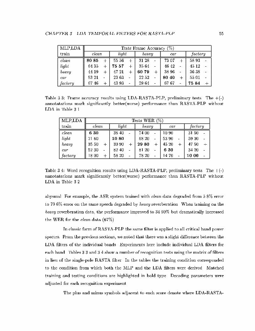
CHAPTER 3. LDA TEMPORAL FILTERS FOR RASTA-PLP 55
MLP,LDA Tests Frame Accuracy (%)train clean light heavy car factory
clean 80.85 + 55.56 + 31.28 - 73.07 + 58.93 -light 64.35 + 75.57 + 35.64 - 46.42 - 45.12 -heavy 44.19 + 47.21 + 60.79 + 38.96 - 36.38 -car 53.21 - 23.63 - 22.52 - 80.40 + 55.01 -factory 67.46 + 43.93 - 29.64 - 67.67 - 75.84 +
Table 3.3: Frame accuracy results using LDA-RASTA-PLP, preliminary tests. The +(-)annotatations mark signi�cantly better(worse) performance than RASTA-PLP withoutLDA in Table 3.1.
MLP,LDA Tests WER (%)train clean light heavy car factory
clean 6.30 36.40 - 74.00 - 10.90 31.50 -light 21.60 10.80 68.20 - 53.90 - 59.30 -heavy 35.50 + 30.90 + 29.80 + 45.20 + 47.50 +car 52.30 - 82.40 - 81.20 - 6.30 34.20 -factory 18.00 + 58.20 - 78.20 - 14.70 - 10.00 -
Table 3.4: Word recognition results using LDA-RASTA-PLP, preliminary tests. The +(-)annotatations mark signi�cantly better(worse) performance than RASTA-PLP withoutLDA in Table 3.2.
abysmal. For example, the ASR system trained with clean data degraded from 5.8% error
to 70.6% error on the same speech degraded by heavy reverberation. When training on the
heavy reverberation data, the performance improved to 34.90% but dramatically increased
the WER for the clean data (67%).
In classic form of RASTA-PLP the same �lter is applied to all critical band power
spectra. From the previous sections, we noted that there was a slight di�erence between the
LDA �lters of the individual bands. Experiments here include individual LDA �lters for
each band. Tables 3.3 and 3.4 show a number of recognition tests using the matrix of �lters
in lieu of the single-pole RASTA �lter. In the tables the training condition corresponded
to the condition from which both the MLP and the LDA �lters were derived. Matched
training and testing conditions are highlighted in bold type. Decoding parameters were
adjusted for each recognition experiment.
The plus and minus symbols adjacent to each score denote where LDA-RASTA-
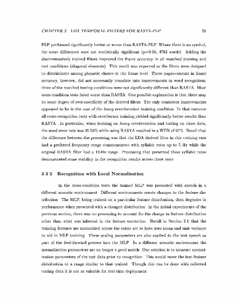
CHAPTER 3. LDA TEMPORAL FILTERS FOR RASTA-PLP 56
PLP performed signi�cantly better or worse than RASTA-PLP. Where there is no symbol,
the score di�erences were not statistically signi�cant (p=0.05, 4763 words). Adding the
discriminatively trained �lters improved the frame accuracy in all matched training and
test conditions (diagonal elements). This result was expected as the �lters were designed
to discriminate among phonetic classes at the frame level. These improvements in frame
accuracy, however, did not necessarily translate into improvements in word recognition;
three of the matched testing conditions were not signi�cantly di�erent than RASTA. Most
cross-condition tests fared worse than RASTA. One possible explanation is that there may
be some degree of over-speci�city of the derived �lters. The only consistent improvements
appeared to be in the case of the heavy reverberation training condition. In that instance
all cross-recognition tests with reverberant training yielded signi�cantly better results than
RASTA. In particular, when training on heavy reverberation and testing on clean data,
the word error rate was 35.50% while using RASTA resulted in a WER of 67%. Recall that
the di�erence between the processing was that the LDA derived �lter in this training case
had a preferred frequency range commensurate with syllabic rates up to 5 Hz while the
original RASTA �lter had a 12-Hz range. Processing that preserved these syllabic rates
demonstrated some stability in the recognition results across these tests.
3.3.2 Recognition with Local Normalization
In the cross-condition tests the trained MLP was presented with speech in a
di�erent acoustic environment. Di�erent environments create changes to the feature dis-
tribution. The MLP, being trained on a particular feature distribution, then degrades in
performance when presented with a changed distribution. In the initial experiments of the
previous section, there was no processing to account for the change in feature distribution
other than what was inherent in the feature extraction. Recall in Section 2.1 that the
training features are normalized across the entire set to have zero mean and unit variance
to aid in MLP training. These scaling parameters are also applied to the test speech as
part of the feed-forward process into the MLP. In a di�erent acoustic environment the
normalization parameters are no longer a good match. One solution is to measure normal-
ization parameters of the test data prior to recognition. This would move the test-feature
distribution to a range similar to that trained. Though this can be done with collected
testing data it is not as suitable for real-time deployment.
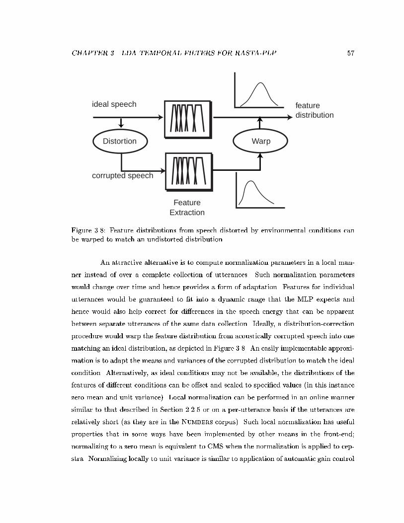
CHAPTER 3. LDA TEMPORAL FILTERS FOR RASTA-PLP 57
FeatureExtraction
Distortion Warp
ideal speech
corrupted speech
featuredistribution
Figure 3.8: Feature distributions from speech distorted by environmental conditions canbe warped to match an undistorted distribution.
An attractive alternative is to compute normalization parameters in a local man-
ner instead of over a complete collection of utterances. Such normalization parameters
would change over time and hence provides a form of adaptation. Features for individual
utterances would be guaranteed to �t into a dynamic range that the MLP expects and
hence would also help correct for di�erences in the speech energy that can be apparent
between separate utterances of the same data collection. Ideally, a distribution-correction
procedure would warp the feature distribution from acoustically corrupted speech into one
matching an ideal distribution, as depicted in Figure 3.8. An easily implementable approxi-
mation is to adapt the means and variances of the corrupted distribution to match the ideal
condition. Alternatively, as ideal conditions may not be available, the distributions of the
features of di�erent conditions can be o�set and scaled to speci�ed values (in this instance
zero mean and unit variance). Local normalization can be performed in an online manner
similar to that described in Section 2.2.5 or on a per-utterance basis if the utterances are
relatively short (as they are in the Numbers corpus). Such local normalization has useful
properties that in some ways have been implemented by other means in the front-end;
normalizing to a zero mean is equivalent to CMS when the normalization is applied to cep-
stra. Normalizing locally to unit variance is similar to application of automatic gain control
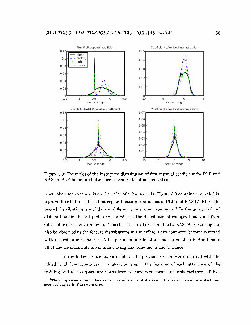
CHAPTER 3. LDA TEMPORAL FILTERS FOR RASTA-PLP 58
1.5 1 0.5 0 0.50
0.02
0.04
0.06
0.08
0.1
0.12First PLP cepstral coefficient
feature range
clean factorylight heavy
10 5 0 50
0.01
0.02
0.03
0.04
0.05Coefficient after local normalization
feature range
1.5 1 0.5 0 0.50
0.02
0.04
0.06
0.08
0.1
0.12First RASTA-PLP cepstral coefficient
feature range10 5 0 5 100
0.01
0.02
0.03
0.04
0.05
0.06
0.07Coefficient after local normalization
feature range
Figure 3.9: Examples of the histogram distribution of �rst cepstral coe�cient for PLP andRASTA-PLP before and after per-utterance local normalization.
where the time constant is on the order of a few seconds. Figure 3.9 contains example his-
togram distributions of the �rst cepstral feature component of PLP and RASTA-PLP. The
pooled distributions are of data in di�erent acoustic environments.2 In the un-normalized
distributions in the left plots one can witness the distributional changes that result from
di�erent acoustic environments. The short-term adaptation due to RASTA processing can
also be observed as the feature distributions in the di�erent environments become centered
with respect to one another. After per-utterance local normalization the distributions in
all of the environments are similar having the same mean and variance.
In the following, the experiments of the previous section were repeated with the
added local (per-utterance) normalization step. The features of each utterance of the
training and test corpora are normalized to have zero mean and unit variance. Tables
2The conspicuous spike in the clean and reverberant distributions in the left column is an artifact fromzero-padding each of the utterances.
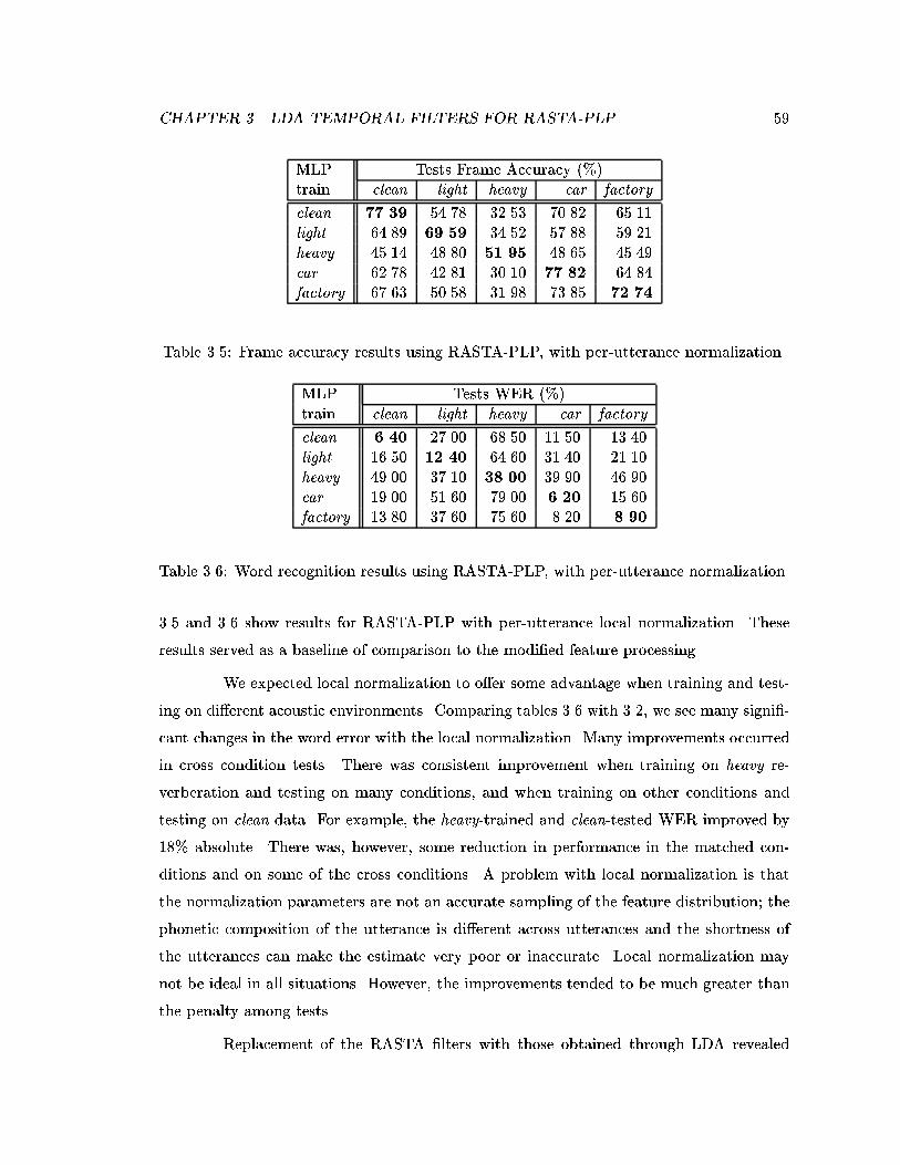
CHAPTER 3. LDA TEMPORAL FILTERS FOR RASTA-PLP 59
MLP Tests Frame Accuracy (%)train clean light heavy car factory
clean 77.39 54.78 32.53 70.82 65.11light 64.89 69.59 34.52 57.88 59.21heavy 45.14 48.80 51.95 48.65 45.49car 62.78 42.81 30.10 77.82 64.84factory 67.63 50.58 31.98 73.85 72.74
Table 3.5: Frame accuracy results using RASTA-PLP, with per-utterance normalization.
MLP Tests WER (%)train clean light heavy car factory
clean 6.40 27.00 68.50 11.50 13.40light 16.50 12.40 64.60 31.40 21.10heavy 49.00 37.10 38.00 39.90 46.90car 19.00 51.60 79.00 6.20 15.60factory 13.80 37.60 75.60 8.20 8.90
Table 3.6: Word recognition results using RASTA-PLP, with per-utterance normalization.
3.5 and 3.6 show results for RASTA-PLP with per-utterance local normalization. These
results served as a baseline of comparison to the modi�ed feature processing.
We expected local normalization to o�er some advantage when training and test-
ing on di�erent acoustic environments. Comparing tables 3.6 with 3.2, we see many signi�-
cant changes in the word error with the local normalization. Many improvements occurred
in cross condition tests. There was consistent improvement when training on heavy re-
verberation and testing on many conditions, and when training on other conditions and
testing on clean data. For example, the heavy-trained and clean-tested WER improved by
18% absolute. There was, however, some reduction in performance in the matched con-
ditions and on some of the cross conditions. A problem with local normalization is that
the normalization parameters are not an accurate sampling of the feature distribution; the
phonetic composition of the utterance is di�erent across utterances and the shortness of
the utterances can make the estimate very poor or inaccurate. Local normalization may
not be ideal in all situations. However, the improvements tended to be much greater than
the penalty among tests.
Replacement of the RASTA �lters with those obtained through LDA revealed
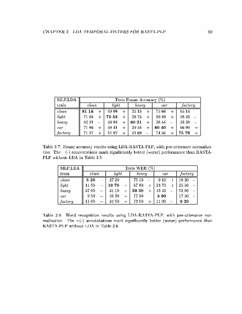
CHAPTER 3. LDA TEMPORAL FILTERS FOR RASTA-PLP 60
MLP,LDA Tests Frame Accuracy (%)train clean light heavy car factory
clean 81.18 + 60.99 + 33.15 + 75.66 + 65.14light 71.04 + 75.53 + 39.75 + 60.49 + 58.45 -heavy 43.21 - 49.94 + 60.21 + 38.54 - 38.38 -car 71.86 + 48.41 + 30.34 + 80.40 + 66.99 +factory 71.17 + 51.97 + 31.69 - 74.50 + 75.79 +
Table 3.7: Frame accuracy results using LDA-RASTA-PLP, with per-utterance normaliza-tion. The +(-) annotatations mark signi�cantly better (worse) performance than RASTA-PLP without LDA in Table 3.5.
MLP,LDA Tests WER (%)train clean light heavy car factory
clean 5.20 + 27.20 75.10 - 9.10 + 19.20 -light 11.50 + 10.70 + 57.80 + 24.70 + 25.50 -heavy 37.00 + 31.10 + 30.30 + 43.50 - 51.80 -car 9.50 + 45.30 + 77.90 5.90 17.50 -factory 11.60 + 34.50 + 73.50 + 11.00 - 9.20
Table 3.8: Word recognition results using LDA-RASTA-PLP, with per-utterance nor-malization. The +(-) annotatations mark signi�cantly better (worse) performance thanRASTA-PLP without LDA in Table 3.6.
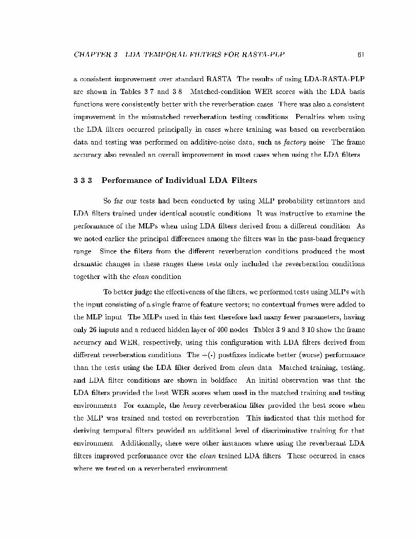
CHAPTER 3. LDA TEMPORAL FILTERS FOR RASTA-PLP 61
a consistent improvement over standard RASTA. The results of using LDA-RASTA-PLP
are shown in Tables 3.7 and 3.8. Matched-condition WER scores with the LDA basis
functions were consistently better with the reverberation cases. There was also a consistent
improvement in the mismatched reverberation testing conditions. Penalties when using
the LDA �lters occurred principally in cases where training was based on reverberation
data and testing was performed on additive-noise data, such as factory noise. The frame
accuracy also revealed an overall improvement in most cases when using the LDA �lters.
3.3.3 Performance of Individual LDA Filters
So far our tests had been conducted by using MLP probability estimators and
LDA �lters trained under identical acoustic conditions. It was instructive to examine the
performance of the MLPs when using LDA �lters derived from a di�erent condition. As
we noted earlier the principal di�erences among the �lters was in the pass-band frequency
range. Since the �lters from the di�erent reverberation conditions produced the most
dramatic changes in these ranges these tests only included the reverberation conditions
together with the clean condition.
To better judge the e�ectiveness of the �lters, we performed tests using MLPs with
the input consisting of a single frame of feature vectors; no contextual frames were added to
the MLP input. The MLPs used in this test therefore had many fewer parameters, having
only 26 inputs and a reduced hidden layer of 400 nodes. Tables 3.9 and 3.10 show the frame
accuracy and WER, respectively, using this con�guration with LDA �lters derived from
di�erent reverberation conditions. The +(-) post�xes indicate better (worse) performance
than the tests using the LDA �lter derived from clean data. Matched training, testing,
and LDA �lter conditions are shown in boldface. An initial observation was that the
LDA �lters provided the best WER scores when used in the matched training and testing
environments. For example, the heavy reverberation �lter provided the best score when
the MLP was trained and tested on reverberation. This indicated that this method for
deriving temporal �lters provided an additional level of discriminative training for that
environment. Additionally, there were other instances where using the reverberant LDA
�lters improved performance over the clean trained LDA �lters. These occurred in cases
where we tested on a reverberated environment.
CHAPTER 3. LDA TEMPORAL FILTERS FOR RASTA-PLP 62
From Table 3.9 we can see that each set of LDA �lters provided similar phone
classi�cation accuracy rates. The accuracy using the heavy LDA �lters, that preferred
lower modulation frequency ranges, were consistently better. In fact, there were numerous
instances where similar or slight improvements in the frame accuracy did not also improve
the WER and in some cases produced the opposite e�ect. For example, when the MLP was
trained and tested on clean data and the heavy LDA �lter was used, the frame accuracy was
higher than the clean LDA �lter but the WER was signi�cantly worse. In a complementary
fashion, when training the MLP with heavy reverberation data and testing on clean data,
the heavy LDA �lter showed lower frame accuracy than the clean LDA �lter, but the WER
was signi�cantly better. Although frame accuracy is generally correlated with WER, a
positive or negative change in the frame accuracy does not guarantee a corresponding
change in word recognition performance. This is not an uncommon observation among
researchers.
Unfortunately, the di�erent LDA �lters did not exhibit as noticeable a positive
e�ect when the MLP was allowed a context of several adjacent acoustic feature frames.
Tables 3.11 and 3.12 show frame accuracy and WER results when using the LDA �lters
in the normal recognition setting. The MLP included 9 frames of acoustic features with
800 hidden units. Here, the di�erent LDA �lters did not exhibit much advantage. That is,
the clean LDA �lter performed about as well the other �lters, often better in mismatched
conditions. The di�erence with the clean LDA �lter in matched training, testing, and LDA
conditions (shown in bold) were not statistically signi�cant.
The purpose of adding discriminatively trained �lters was to add a discrimina-
tive component along the temporal dimension in addition to the frequency-related di-
rection. With an acoustic context of 9 frames, the MLP had access to about 100 ms
of acoustic information. The MLP, being non-linear and discriminatively trained, could
therefore incorporate temporal processing and in some sense mimic certain properties of
the temporal LDA �lters. The reverberation-trained LDA �lters were linear and more
frequency restrictive and may have discarded information exploitable by the MLP. Fur-
ther, the reverberation-derived �lters exhibited a broader temporal response and may have
brought in more acoustic context into the MLP than was necessary. Earlier experiments
by ICSI researchers conducted by varying the input context of the MLP reveal that in-
creasing the number of input feature frames from a single frame improves word recognition
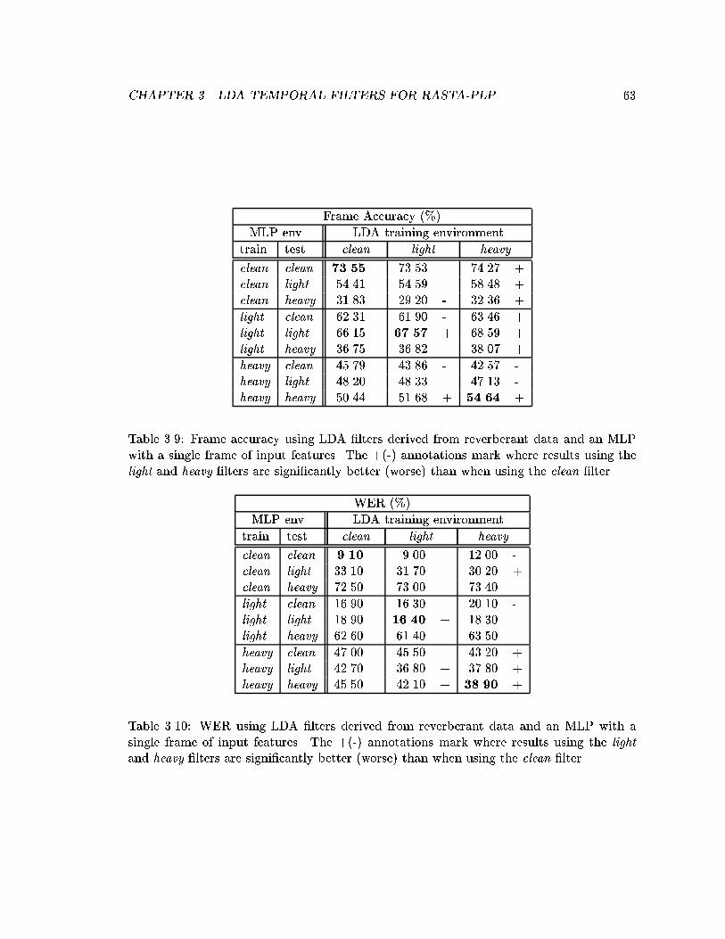
CHAPTER 3. LDA TEMPORAL FILTERS FOR RASTA-PLP 63
Frame Accuracy (%)
MLP env. LDA training environment
train test clean light heavy
clean clean 73.55 73.53 74.27 +clean light 54.41 54.59 58.48 +clean heavy 31.83 29.20 - 32.36 +
light clean 62.31 61.90 - 63.46 +light light 66.15 67.57 + 68.59 +light heavy 36.75 36.82 38.07 +
heavy clean 45.79 43.86 - 42.57 -heavy light 48.20 48.33 47.13 -heavy heavy 50.44 51.68 + 54.64 +
Table 3.9: Frame accuracy using LDA �lters derived from reverberant data and an MLPwith a single frame of input features. The +(-) annotations mark where results using thelight and heavy �lters are signi�cantly better (worse) than when using the clean �lter.
WER (%)
MLP env. LDA training environment
train test clean light heavy
clean clean 9.10 9.00 12.00 -clean light 33.10 31.70 30.20 +clean heavy 72.50 73.00 73.40
light clean 16.90 16.30 20.10 -light light 18.90 16.40 + 18.30light heavy 62.60 61.40 63.50
heavy clean 47.00 45.50 43.20 +heavy light 42.70 36.80 + 37.80 +heavy heavy 45.50 42.10 + 38.90 +
Table 3.10: WER using LDA �lters derived from reverberant data and an MLP with asingle frame of input features. The +(-) annotations mark where results using the light
and heavy �lters are signi�cantly better (worse) than when using the clean �lter.
CHAPTER 3. LDA TEMPORAL FILTERS FOR RASTA-PLP 64
scores. However, the performance begins to degrade when the context becomes too wide
[81, 116]. Previous tests have indicated that a context window of about 9 frames yields
good classi�cation results. This also covers the breadth of the active region of the impulse
responses of the LDA �lters.
3.4 Discussion
We see that a di�erence in the acoustic environment can have a highly detrimental
e�ect on recognition performance. Merely training the probability estimator on the new
condition will improve results dramatically. In addition to discriminative training of an
MLP to produce posterior estimates, we also attempted to add another level of trained
discriminability along the temporal dimension. LDA provides an interesting mechanism
for determining the proper temporal �lters in RASTA-PLP. Not only does it verify some
of the intuition behind the design of the original RASTA �lter but it adds a direct and
\automatic" means of determining and analyzing the discriminant basis functions along
the temporal dimension. Since these �lters were determined from a collection of data
there remains a danger that they may only be applicable to speci�c situations. This was
one of the reasons for using a speech corpus for �lter derivation di�erent from the one
used for word-recognition tests. However, another complication exists in that the units for
deriving the discriminant �lters may not be optimal for the overall task. The LDA �lters
were derived using phonetic labels from hand transcriptions. Therefore, the �lters in some
sense sought to improve phonetic classi�cation of these labels on a frame by frame basis.
This does not ensure that the overall word recognition will also be improved. It can be
argued that a good frame accuracy of phone classes is necessary for good word recognition.
However, an improvement in frame accuracy is not a su�cient condition for improved word
recognition. A further discussion of this appears in Chapter 4 and Appendix E.
The principal di�erence between the �lters derived from di�erent conditions was
in the width and range of the pass-band. For increasingly noisy environments there was
a tendency for the �lters to prefer the lower-modulation frequency range. Additive noise
did not appear to exhibit as much of a change as the addition of reverberation. The
reverberation-trained �lters may therefore not be as helpful for additive-noise cases. Our
results showed a consistent problem when training on the reverberation environment and
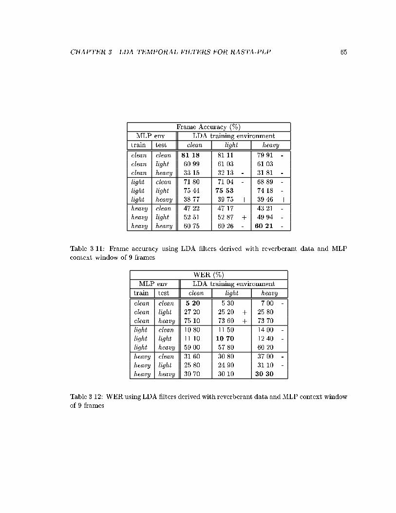
CHAPTER 3. LDA TEMPORAL FILTERS FOR RASTA-PLP 65
Frame Accuracy (%)
MLP env. LDA training environment
train test clean light heavy
clean clean 81.18 81.11 79.91 -clean light 60.99 61.03 61.03clean heavy 33.15 32.13 - 31.81 -
light clean 71.80 71.04 - 68.89 -light light 75.44 75.53 74.18 -light heavy 38.77 39.75 + 39.46 +
heavy clean 47.22 47.17 43.21 -heavy light 52.51 52.87 + 49.94 -heavy heavy 60.75 60.26 - 60.21 -
Table 3.11: Frame accuracy using LDA �lters derived with reverberant data and MLPcontext window of 9 frames.
WER (%)
MLP env. LDA training environment
train test clean light heavy
clean clean 5.20 5.30 7.00 -clean light 27.20 25.20 + 25.80clean heavy 75.10 73.60 + 73.70
light clean 10.80 11.50 14.00 -light light 11.10 10.70 12.40 -light heavy 59.00 57.80 60.20
heavy clean 31.60 30.80 37.00 -heavy light 25.80 24.90 31.10 -heavy heavy 30.70 30.10 30.30
Table 3.12: WER using LDA �lters derived with reverberant data and MLP context windowof 9 frames.
CHAPTER 3. LDA TEMPORAL FILTERS FOR RASTA-PLP 66
testing on the added noise environment, and vice versa. Since the di�erence was rather
pronounced, it may be necessary to retain multiple front-end and acoustic modeling stages
for handling each environment until the di�erences can be reconciled by other means. A
suitable combination of the acoustic processing stages may be employed when the target
environment is unknown. One e�ect of the added environments is a change in the trajec-
tory of the critical-band energy. As a result, the variance patterns of the trajectories are
altered, typically reduced to some degree. Added noise and room reverberation change
the distribution and the covariance in a di�erent manner. Since the LDA calculation is
based upon covariance calculations, we expect some modi�cation of the basis functions if
the environments a�ect the within- and between-class covariances to a di�erent degree.
The heavy reverberation case caused a severe attening of the critical-band tra-
jectory and hence was associated with smaller variance. This case resulted in the most
limiting frequency response, keeping frequencies between 1 and 5 Hz in the principal LDA
component. Since this range was commensurate with syllabic rates we also conducted some
tests where we derived LDA �lters using syllable targets instead of phone targets. These
are described in in Appendix C. One of the results of using syllables as targets was that
the �lter impulse responses were broader and also kept a pass-band of about 1 to 5 Hz
and bore strong similarity to the �lters derived in severe reverberation. Further, this rate
appeared stable regardless of the acoustic environment added to the data. This appears
to support the bene�t of analyzing wider analysis windows using a more syllabic rate for
perceptual stability. In noisy environments phonetic identity often becomes obscured. A
back-o� strategy to wider temporal integration and higher-level knowledge may be em-
ployed to aid in decoding the utterance. Further discussion and work on the use of syllable
or syllable-like information for speech recognition can be found in [39, 117, 120, 101].
Since the responses of the LDA �lters across all frequency bands were similar,
with some di�erences among bands, we also experimented with applying a single �lter to
all of the frequency bands just as the standard RASTA-PLP does. This single �lter was
the averaged response of all of the individual responses. Pilot tests with these averaged
�lters yielded results that were consistent with the tests here, though with slightly worse
performance. Subtle di�erences among the responses of the individual band �lters account
for this. However, di�erent types of phone classes carry di�erent temporal properties and
occupy di�erent frequency ranges. For example, vocalic phones principally occupy the lower
CHAPTER 3. LDA TEMPORAL FILTERS FOR RASTA-PLP 67
frequency bands and have some durational di�erences from other phones such as stops and
plosives that have a shorter duration but span higher frequencies. Using a single bank of
�lters designed to discriminate among all phones may in the future be further augmented
by �lters designed to discriminate among certain classes of phones similar to the TRAPS
�lters derived by Sharma [99, 98, 51]. TRAPS �lters are matched �lters derived from
averaging the temporal trajectories of phone classes and have been used successfully in an
articulatory feature based system and in multi-stream systems. Many options for temporal
�ltering exist. LDA provides a relatively simple method of obtaining �lters derived from
a discriminative criterion. It further allows us to examine the trends in the modulation
spectrum that carry phone discriminative information in the presence of signal degradation
due to acoustic environments.
68
Chapter 4
LDA temporal �lters with PLP
and MSG
In the previous chapter, LDA was applied individually to the logarithm of the
critical-band trajectories. In RASTA-PLP, �ltering in the log-power spectral domain al-
lowed for transforming convolutional noise into additive noise, to which a linear �lter can
be applied. Applying LDA in this domain produced basis �lters with consistent properties.
It was demonstrated that using discriminatively trained LDA �lters could further im-
prove classi�cation and recognition performance. Since there are situations when di�erent
feature-extraction algorithms will perform better it was worthwhile to explore the poten-
tial enhancement of other algorithms with the temporal LDA technique. In this chapter
we explore the application of LDA �lter design to two other preprocessing con�gurations,
PLP-cepstra and MSG.
4.1 Logarithm of the Power Spectra
First we must consider where application of LDA is suitable. RASTA-PLP applies
temporal �ltering to compressed power spectra. The compressing function is memoryless
and is usually a logarithm, though other functions, such as a root power, can also be used.
Other preprocessing strategies such as MSG use a root power in lieu of a logarithm applied
to the power spectral estimates. The question arises as to which domain is best or whether
the di�erence in domain is important. For the application of LDA we �nd that the domain
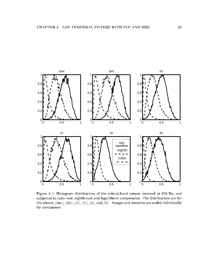
CHAPTER 4. LDA TEMPORAL FILTERS WITH PLP AND MSG 69
0 0.5 10
0.2
0.4
0.6
0.8
1/ow/
0 0.5 10
0.2
0.4
0.6
0.8
1/eh/
0 0.5 10
0.2
0.4
0.6
0.8
1/n/
0 0.5 10
0.2
0.4
0.6
0.8
1/r/
0 0.5 10
0.2
0.4
0.6
0.8
1/s/
0 0.5 10
0.2
0.4
0.6
0.8
1/k/
log
eighth
cube
Figure 4.1: Histogram distributions of the critical-band output centered at 570 Hz, andsubjected to cube-root, eighth-root and logarithmic compression. The distributions are forthe phones /ow/, /eh/, /n/, /r/, /s/, and /k/. Ranges and densities are scaled individuallyfor comparison.
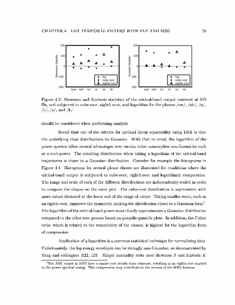
CHAPTER 4. LDA TEMPORAL FILTERS WITH PLP AND MSG 70
/ow/ /eh/ /n/ /r/ /s/ /k/200
100
0
100
200
Ske
wne
ss S
tatis
tic
log cube root eighth root
/ow/ /eh/ /n/ /r/ /s/ /k/200
100
0
100
200
Kur
tosi
s S
tatis
tic
log cube root eighth root
Figure 4.2: Skewness and Kurtosis statistics of the critical-band output centered at 570Hz, and subjected to cube root, eighth root, and logarithm for the phones /ow/, /eh/, /n/,/r/, /s/, and /k/.
should be considered when performing analysis.
Recall that one of the criteria for optimal linear separability using LDA is that
the underlying class distributions be Gaussian. With that in mind, the logarithm of the
power spectra o�ers several advantages over certain other memoryless non-linearities such
as a root-power. The resulting distribution when taking a logarithm of the critical-band
trajectories is closer to a Gaussian distribution. Consider for example the histograms in
Figure 4.1. Histograms for several phone classes are illustrated for conditions where the
critical-band output is subjected to cube-root, eighth-root and logarithmic compression.
The range and scale of each of the di�erent distributions are independently scaled in order
to compare the shapes on the same plot. The cube-root distribution is asymmetric with
more values clustered at the lower end of the range of values. Taking smaller roots, such as
an eighth-root, improves the symmetry, making the distribution closer to a Gaussian form1.
The logarithm of the critical-band power most closely approximates a Gaussian distribution
compared to the other root powers based on quantile-quantile plots. In addition, the Fisher
ratio, which is related to the separability of the classes, is highest for the logarithm form
of compression.
Application of a logarithm is a common statistical technique for normalizing data.
Unfortunately, the log-energy envelopes can be strongly non-Gaussian, as demonstrated by
Yang and colleagues [122, 121]. Simple normality tests used skewness S and kurtosis K
1The AGC stages in MSG have a square root steady state response, resulting in an eighth-root appliedto the power spectral energy. This compression may contribute to the success of the MSG features.
CHAPTER 4. LDA TEMPORAL FILTERS WITH PLP AND MSG 71
statistics:
S =1p6T �̂3
TXt=1
(xt � �̂)3 (4.1)
K =1p
24T �̂4
TXt=1
(xt � �̂)4 �s3T
8(4.2)
where �̂ and �̂ are the sample mean and standard deviations of envelope xt. S and K
are standard normal under the null hypothesis. Whereas the total pooled distribution is
strongly non-Gaussian, phonetic class subsets appear to be better behaved. Statistics for
several phones, subjected to logarithm, cube-root, and eighth-root compression are shown
in Figure 4.2. From this plot, the logarithmic data is closer to the critical signi�cance range
of�2:58 (p=0.01). The logarithm does not support the Gaussianity null hypothesis in many
tests but is demonstrably superior to the cube- and eighth-root forms of compression. The
logarithm also o�ers some mathematical advantages over the root powers. As mentioned
in Section 2.2.4, the logarithm provides justi�cation for transforming convolutional noise
into additive noise. Log-domain �ltering can be interpreted as short-term adaptation or as
some form of automatic gain control. Additionally, the spectral distribution resulting from
a logarithm is shape-invariant to both scaling and powers of the input, whereas the root
power is only shape-invariant to scaling of the input. Scaling the input by a constant factor
merely adjusts the span of the domain of the distribution for the root-powers and shifts
the domain for the logarithm since log(aX) = log(a) + log(X). Observing the logarithmic
property that log(Xp) = p log(X), we also see that powers of the input also appear as a
scaling constant and therefore only a�ect the span of the distribution; the shape of the
distribution remains intact. To reiterate, a scale and power operation results in a shift and
scale operation after a logarithm. When the resulting distribution is Gaussian, such a shift
and scale amounts to adjusting the mean and the variance while preserving the Gaussian
nature of the distribution.
4.2 Delta Calculation with Perceptual Linear Prediction
Numerous tests have revealed that RASTA processing aids in reducing the chan-
nel variability introduced by a change in microphone or telephone line [82, 50]. Since the
typical response of these channels is short enough to be contained within a single analy-
sis window, this form of convolutional noise can be dealt with using RASTA �ltering in
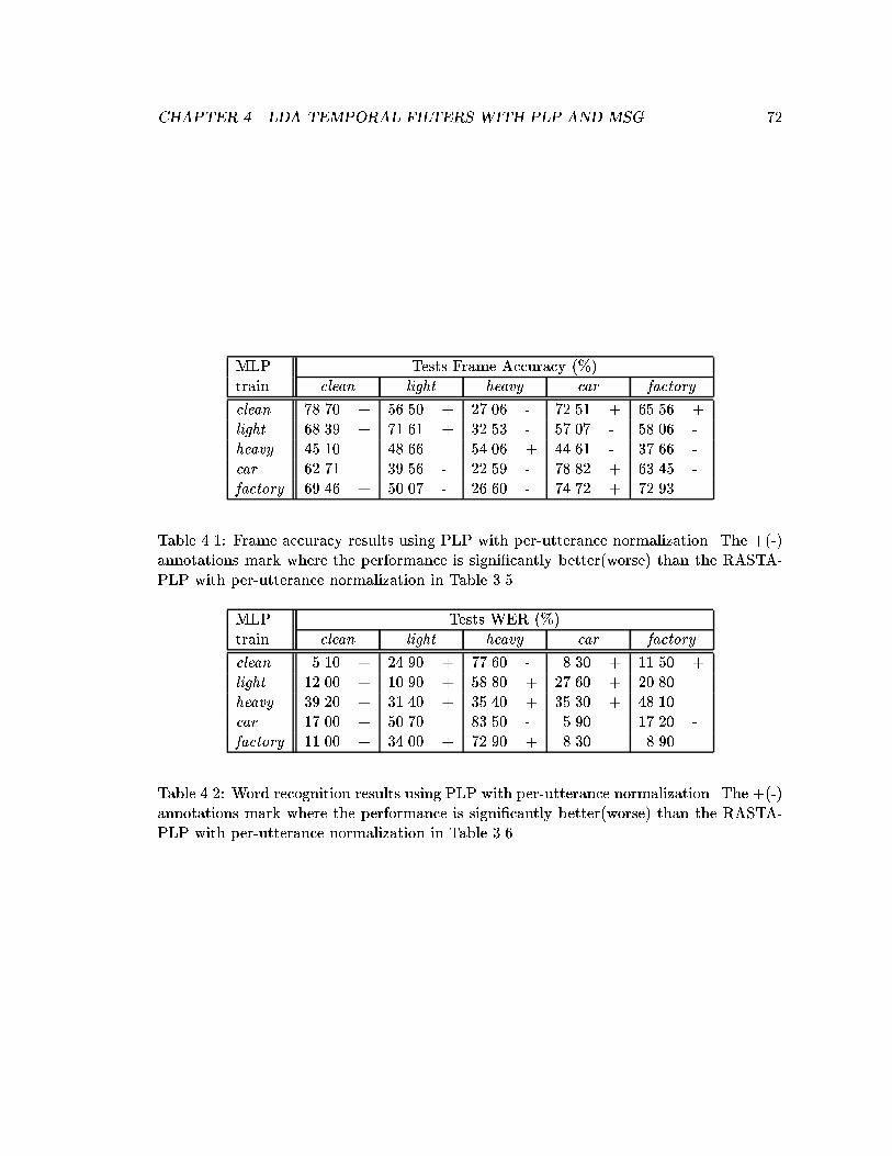
CHAPTER 4. LDA TEMPORAL FILTERS WITH PLP AND MSG 72
MLP Tests Frame Accuracy (%)train clean light heavy car factory
clean 78.70 + 56.50 + 27.06 - 72.51 + 65.56 +light 68.39 + 71.61 + 32.53 - 57.07 - 58.06 -heavy 45.10 48.66 54.06 + 44.61 - 37.66 -car 62.71 39.56 - 22.59 - 78.82 + 63.45 -factory 69.46 + 50.07 - 26.60 - 74.72 + 72.93
Table 4.1: Frame accuracy results using PLP with per-utterance normalization. The +(-)annotations mark where the performance is signi�cantly better(worse) than the RASTA-PLP with per-utterance normalization in Table 3.5.
MLP Tests WER (%)train clean light heavy car factory
clean 5.10 + 24.90 + 77.60 - 8.30 + 11.50 +light 12.00 + 10.90 + 58.80 + 27.60 + 20.80heavy 39.20 + 31.40 + 35.40 + 35.30 + 48.10car 17.00 + 50.70 83.50 - 5.90 17.20 -factory 11.00 + 34.00 + 72.90 + 8.30 8.90
Table 4.2: Word recognition results using PLP with per-utterance normalization. The +(-)annotations mark where the performance is signi�cantly better(worse) than the RASTA-PLP with per-utterance normalization in Table 3.6.
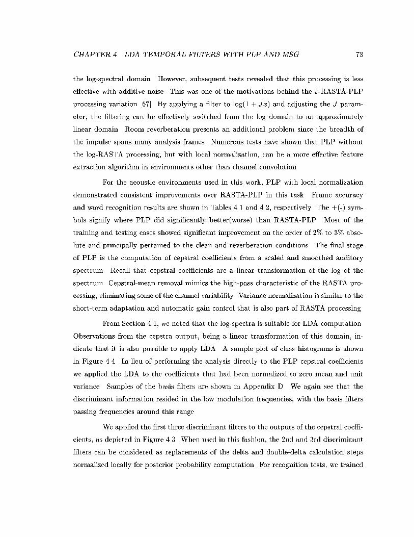
CHAPTER 4. LDA TEMPORAL FILTERS WITH PLP AND MSG 73
the log-spectral domain. However, subsequent tests revealed that this processing is less
e�ective with additive noise. This was one of the motivations behind the J-RASTA-PLP
processing variation [67]. By applying a �lter to log(1 + Jx) and adjusting the J param-
eter, the �ltering can be e�ectively switched from the log domain to an approximately
linear domain. Room reverberation presents an additional problem since the breadth of
the impulse spans many analysis frames. Numerous tests have shown that PLP without
the log-RASTA processing, but with local normalization, can be a more e�ective feature
extraction algorithm in environments other than channel convolution.
For the acoustic environments used in this work, PLP with local normalization
demonstrated consistent improvements over RASTA-PLP in this task. Frame accuracy
and word recognition results are shown in Tables 4.1 and 4.2, respectively. The +(-) sym-
bols signify where PLP did signi�cantly better(worse) than RASTA-PLP. Most of the
training and testing cases showed signi�cant improvement on the order of 2% to 3% abso-
lute and principally pertained to the clean and reverberation conditions. The �nal stage
of PLP is the computation of cepstral coe�cients from a scaled and smoothed auditory
spectrum. Recall that cepstral coe�cients are a linear transformation of the log of the
spectrum. Cepstral-mean removal mimics the high-pass characteristic of the RASTA pro-
cessing, eliminating some of the channel variability. Variance normalization is similar to the
short-term adaptation and automatic gain control that is also part of RASTA processing.
From Section 4.1, we noted that the log-spectra is suitable for LDA computation.
Observations from the cepstra output, being a linear transformation of this domain, in-
dicate that it is also possible to apply LDA. A sample plot of class histograms is shown
in Figure 4.4. In lieu of performing the analysis directly to the PLP cepstral coe�cients
we applied the LDA to the coe�cients that had been normalized to zero mean and unit
variance. Samples of the basis �lters are shown in Appendix D. We again see that the
discriminant information resided in the low modulation frequencies, with the basis �lters
passing frequencies around this range.
We applied the �rst three discriminant �lters to the outputs of the cepstral coe�-
cients, as depicted in Figure 4.3. When used in this fashion, the 2nd and 3rd discriminant
�lters can be considered as replacements of the delta and double-delta calculation steps
normalized locally for posterior probability computation. For recognition tests, we trained
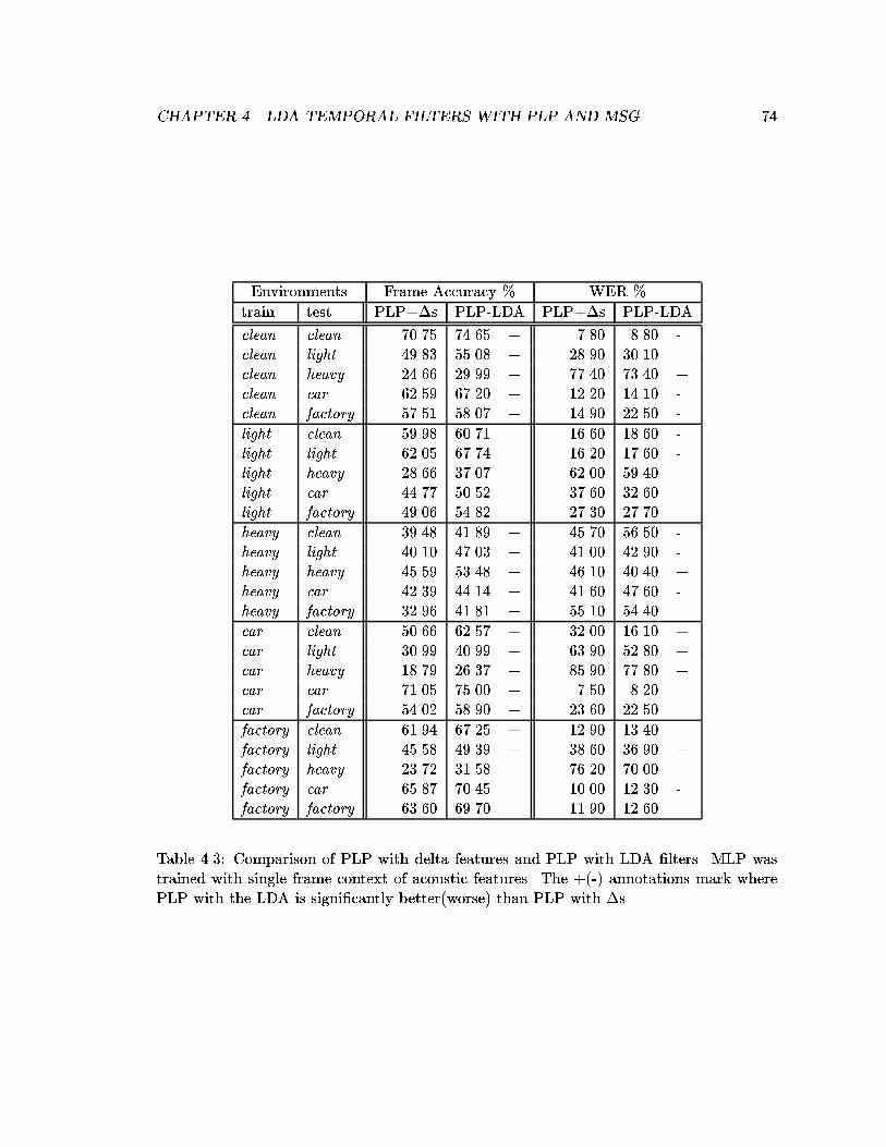
CHAPTER 4. LDA TEMPORAL FILTERS WITH PLP AND MSG 74
Environments Frame Accuracy % WER %
train test PLP+�s PLP-LDA PLP+�s PLP-LDA
clean clean 70.75 74.65 + 7.80 8.80 -clean light 49.83 55.08 + 28.90 30.10clean heavy 24.66 29.99 + 77.40 73.40 +clean car 62.59 67.20 + 12.20 14.10 -clean factory 57.51 58.07 + 14.90 22.50 -
light clean 59.98 60.71 + 16.60 18.60 -light light 62.05 67.74 + 16.20 17.60 -light heavy 28.66 37.07 + 62.00 59.40 +light car 44.77 50.52 + 37.60 32.60 +light factory 49.06 54.82 + 27.30 27.70
heavy clean 39.48 41.89 + 45.70 56.50 -heavy light 40.10 47.03 + 41.00 42.90 -heavy heavy 45.59 53.48 + 46.10 40.40 +heavy car 42.39 44.14 + 41.60 47.60 -heavy factory 32.96 41.81 + 55.10 54.40
car clean 50.66 62.57 + 32.00 16.10 +car light 30.99 40.99 + 63.90 52.80 +car heavy 18.79 26.37 + 85.90 77.80 +car car 71.05 75.00 + 7.50 8.20car factory 54.02 58.90 + 23.60 22.50
factory clean 61.94 67.25 + 12.90 13.40factory light 45.58 49.39 + 38.60 36.90 +factory heavy 23.72 31.58 + 76.20 70.00 +factory car 65.87 70.45 + 10.00 12.30 -factory factory 63.60 69.70 + 11.90 12.60
Table 4.3: Comparison of PLP with delta features and PLP with LDA �lters. MLP wastrained with single frame context of acoustic features. The +(-) annotations mark wherePLP with the LDA is signi�cantly better(worse) than PLP with �s.
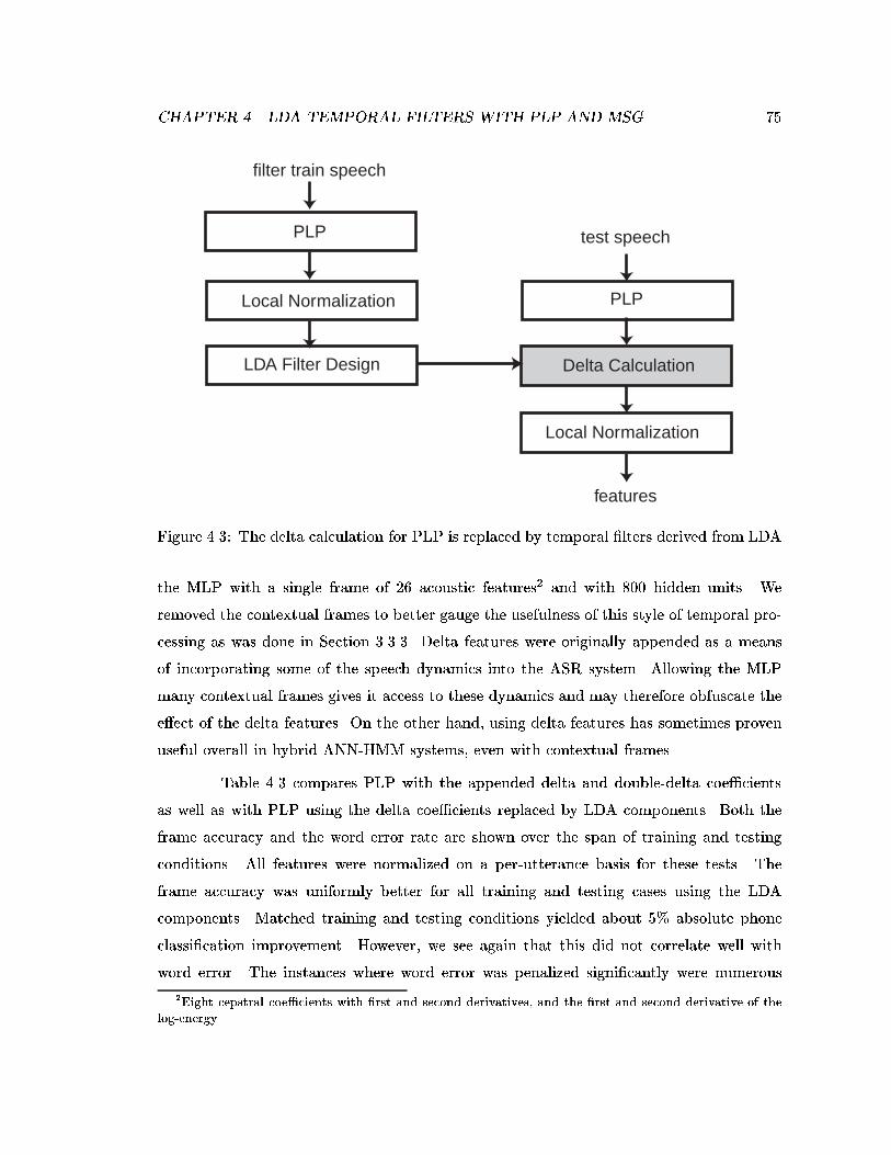
CHAPTER 4. LDA TEMPORAL FILTERS WITH PLP AND MSG 75
LDA Filter Design
filter train speech
test speech
features
PLP
Local Normalization
Delta Calculation
PLPLocal Normalization
Figure 4.3: The delta calculation for PLP is replaced by temporal �lters derived from LDA
the MLP with a single frame of 26 acoustic features2 and with 800 hidden units. We
removed the contextual frames to better gauge the usefulness of this style of temporal pro-
cessing as was done in Section 3.3.3. Delta features were originally appended as a means
of incorporating some of the speech dynamics into the ASR system. Allowing the MLP
many contextual frames gives it access to these dynamics and may therefore obfuscate the
e�ect of the delta features. On the other hand, using delta features has sometimes proven
useful overall in hybrid ANN-HMM systems, even with contextual frames.
Table 4.3 compares PLP with the appended delta and double-delta coe�cients
as well as with PLP using the delta coe�cients replaced by LDA components. Both the
frame accuracy and the word error rate are shown over the span of training and testing
conditions. All features were normalized on a per-utterance basis for these tests. The
frame accuracy was uniformly better for all training and testing cases using the LDA
components. Matched training and testing conditions yielded about 5% absolute phone
classi�cation improvement. However, we see again that this did not correlate well with
word error. The instances where word error was penalized signi�cantly were numerous
2Eight cepstral coe�cients with �rst and second derivatives, and the �rst and second derivative of thelog-energy.
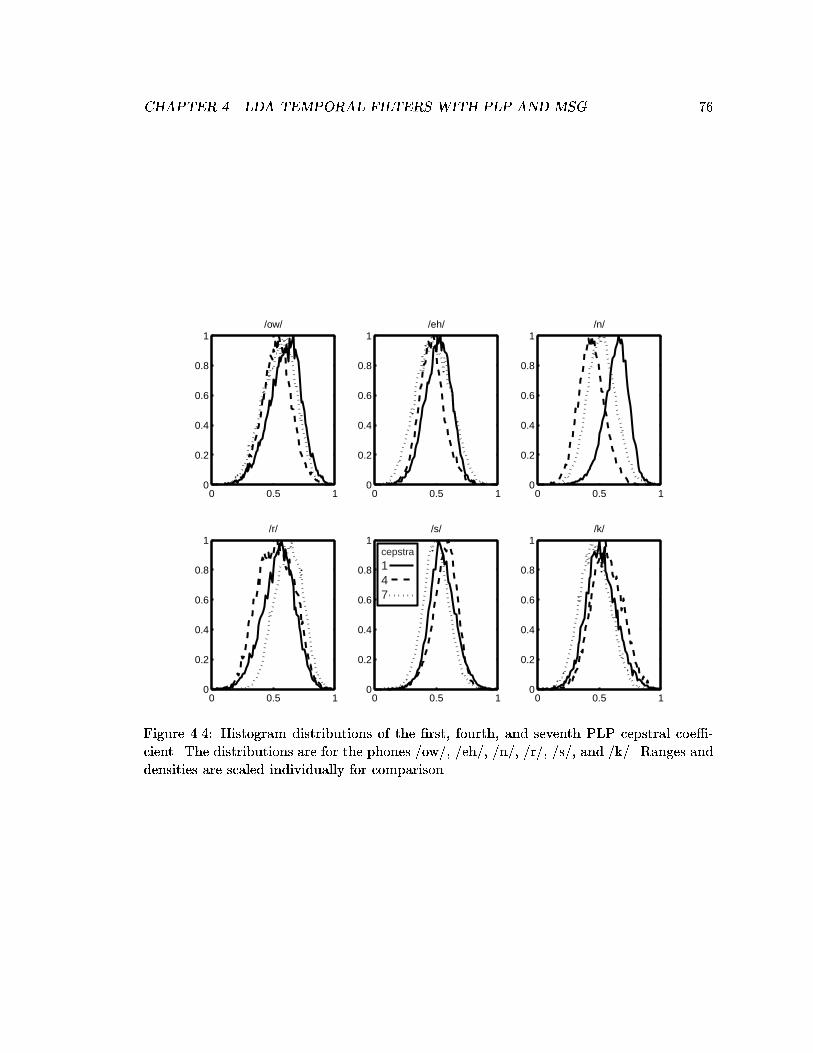
CHAPTER 4. LDA TEMPORAL FILTERS WITH PLP AND MSG 76
0 0.5 10
0.2
0.4
0.6
0.8
1/ow/
0 0.5 10
0.2
0.4
0.6
0.8
1/eh/
0 0.5 10
0.2
0.4
0.6
0.8
1/n/
0 0.5 10
0.2
0.4
0.6
0.8
1/r/
0 0.5 10
0.2
0.4
0.6
0.8
1/s/
0 0.5 10
0.2
0.4
0.6
0.8
1/k/
cepstra
147
Figure 4.4: Histogram distributions of the �rst, fourth, and seventh PLP cepstral coe�-cient. The distributions are for the phones /ow/, /eh/, /n/, /r/, /s/, and /k/. Ranges anddensities are scaled individually for comparison.
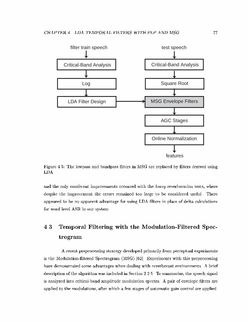
CHAPTER 4. LDA TEMPORAL FILTERS WITH PLP AND MSG 77
Critical-Band Analysis
Log
LDA Filter Design
Critical-Band Analysis
filter train speech test speech
features
Square Root
MSG Envelope Filters
AGC Stages
Online Normalization
Figure 4.5: The lowpass and bandpass �lters in MSG are replaced by �lters derived usingLDA.
and the only consistent improvements occurred with the heavy reverberation tests, where
despite the improvement the errors remained too large to be considered useful. There
appeared to be no apparent advantage for using LDA �lters in place of delta calculations
for word level ASR in our system.
4.3 Temporal Filtering with the Modulation-Filtered Spec-
trogram
A recent preprocessing strategy developed primarily from perceptual experiments
is the Modulation-�ltered Spectrogram (MSG) [62]. Experiments with this preprocessing
have demonstrated some advantages when dealing with reverberant environments. A brief
description of the algorithm was included in Section 2.2.5. To summarize, the speech signal
is analyzed into critical-band amplitude modulation spectra. A pair of envelope �lters are
applied to the modulations, after which a few stages of automatic gain control are applied.
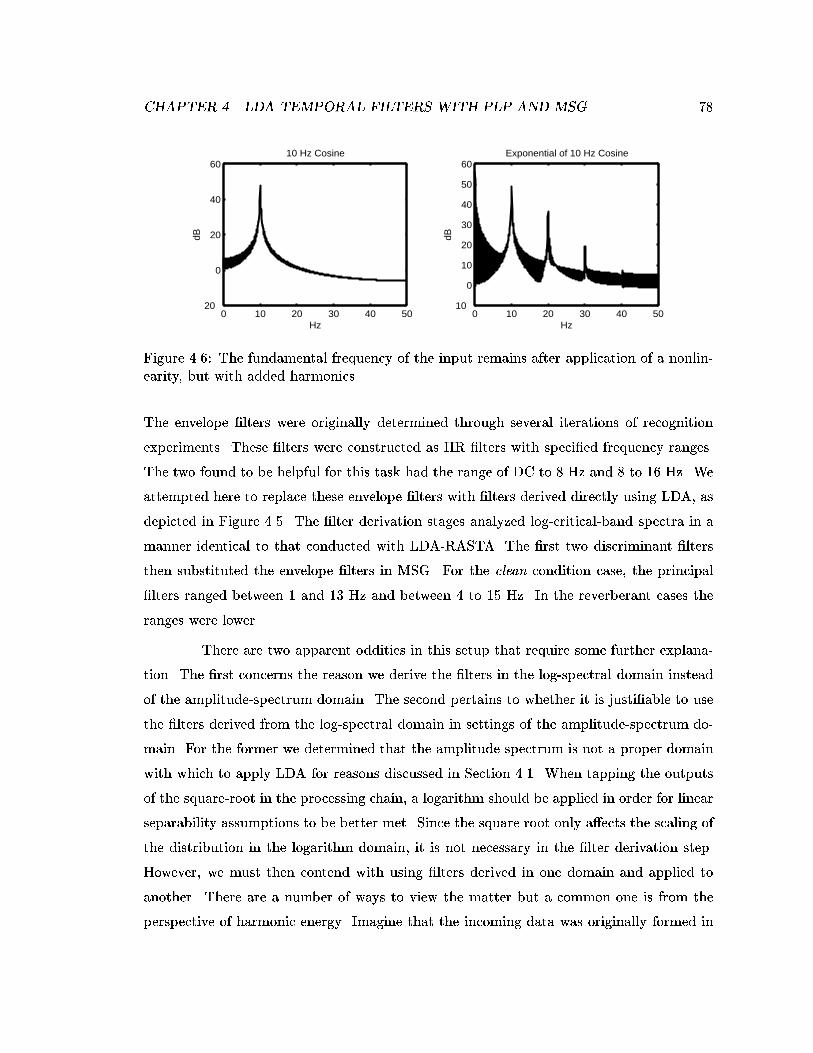
CHAPTER 4. LDA TEMPORAL FILTERS WITH PLP AND MSG 78
0 10 20 30 40 5020
0
20
40
60
Hz
dB
10 Hz Cosine
0 10 20 30 40 5010
0
10
20
30
40
50
60
Hz
dB
Exponential of 10 Hz Cosine
Figure 4.6: The fundamental frequency of the input remains after application of a nonlin-earity, but with added harmonics.
The envelope �lters were originally determined through several iterations of recognition
experiments. These �lters were constructed as IIR �lters with speci�ed frequency ranges.
The two found to be helpful for this task had the range of DC to 8 Hz and 8 to 16 Hz. We
attempted here to replace these envelope �lters with �lters derived directly using LDA, as
depicted in Figure 4.5. The �lter derivation stages analyzed log-critical-band spectra in a
manner identical to that conducted with LDA-RASTA. The �rst two discriminant �lters
then substituted the envelope �lters in MSG. For the clean condition case, the principal
�lters ranged between 1 and 13 Hz and between 4 to 15 Hz. In the reverberant cases the
ranges were lower.
There are two apparent oddities in this setup that require some further explana-
tion. The �rst concerns the reason we derive the �lters in the log-spectral domain instead
of the amplitude-spectrum domain. The second pertains to whether it is justi�able to use
the �lters derived from the log-spectral domain in settings of the amplitude-spectrum do-
main. For the former we determined that the amplitude spectrum is not a proper domain
with which to apply LDA for reasons discussed in Section 4.1. When tapping the outputs
of the square-root in the processing chain, a logarithm should be applied in order for linear
separability assumptions to be better met. Since the square root only a�ects the scaling of
the distribution in the logarithm domain, it is not necessary in the �lter derivation step.
However, we must then contend with using �lters derived in one domain and applied to
another. There are a number of ways to view the matter but a common one is from the
perspective of harmonic energy. Imagine that the incoming data was originally formed in
CHAPTER 4. LDA TEMPORAL FILTERS WITH PLP AND MSG 79
the log-spectral domain to which an exponential was applied prior to �ltering. In the fre-
quency domain the e�ect of applying an exponential (and a large class of other memoryless
non-linearities) is the introduction of harmonics. For example, Figure 4.6 shows the mag-
nitude frequency response of a 10-Hz cosine along side the magnitude frequency response
after the cosine is exponentiated. The non-linearity preserves the basic uctuation of 10
Hz but additional harmonics are created at integer multiples of this frequency. Other than
the DC component, the main harmonic at 20 Hz in this case is 10 dB below the 10-Hz
fundamental. If the signal of interest is in a narrow enough frequency range, the original
signal may be extracted through �ltering. This frequency component will be a�ected by
the presence of other frequencies however. The presence of another frequency component
at 5 Hz would place a main harmonic at 10 Hz. Additionally, owing to the periodic nature
of the discrete time domain, the presence of frequencies at 35 Hz and 45 Hz also place
a harmonic at 10 Hz. Fortunately, the energy at these latter frequencies is small in the
modulation spectrum of speech. More generally, the result of this nonlinearity would be a
raising of the noise oor in a signal-dependent fashion.
From this perspective, the LDA �lters in this case may be interpreted a little
more generally in that they may be applied to modulation trajectories that are warped
by a memoryless nonlinearity. The principal LDA �lters preserved the lower modulation
frequencies up to 16 Hz. This is commensurate with the modulation rates of speech.
Experiments by Drullman et. al. [27], Arai et. al. [5] and Silipo et. al. [105] indicate that
modulation frequencies in this range are crucial for the intelligibility of speech. What is
important is the preservation of the rates with which speech modulates.
When we replaced the envelope �lters in MSG with those derived directly from
data, we obtained results that were similar to the e�ect when we replaced PLP delta coef-
�cients with LDA-�ltered coe�cients. We obtained a consistent improvement in the frame
accuracy in both matched and mismatched training and testing conditions. However, this
consistent improvement in frame accuracy was again not re ected in the word-recognition
error. There were many cases where an improvement in frame accuracy resulted in a corre-
sponding penalty in word-recognition performance. These tests were conducted using the
larger connected MLP with 9 frames of input context and 800 hidden units. Results were
similar when using a single frame of acoustic features.
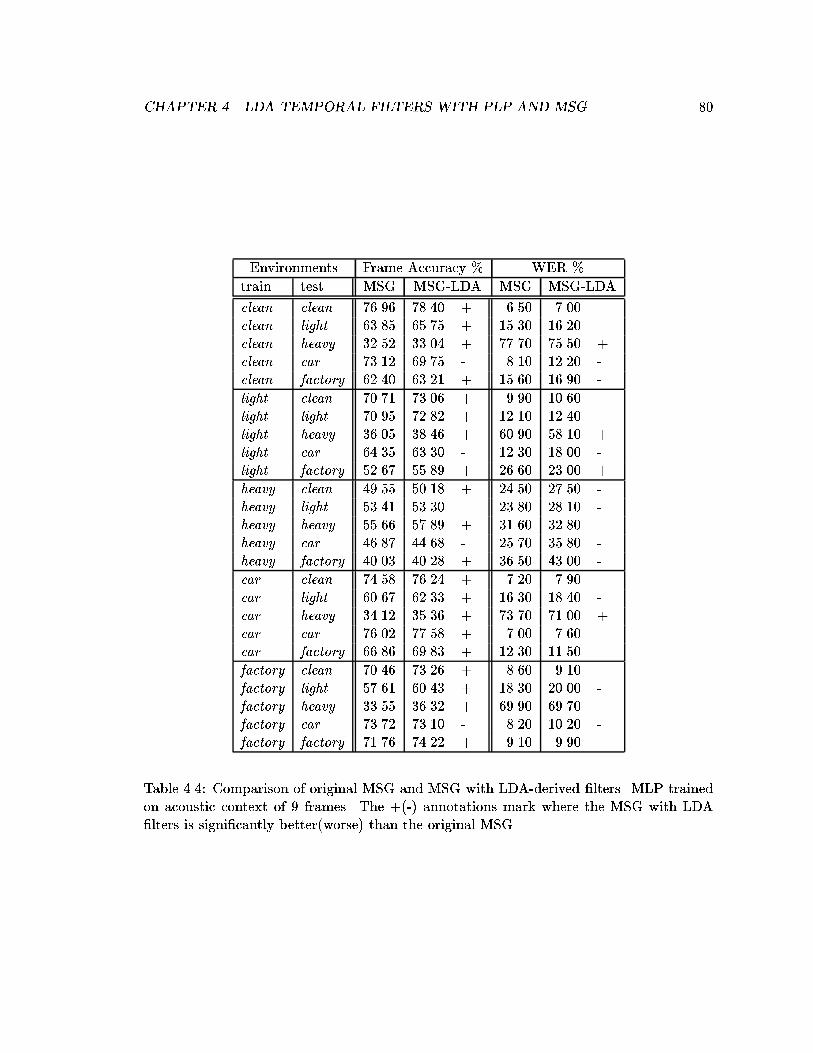
CHAPTER 4. LDA TEMPORAL FILTERS WITH PLP AND MSG 80
Environments Frame Accuracy % WER %
train test MSG MSG-LDA MSG MSG-LDA
clean clean 76.96 78.40 + 6.50 7.00clean light 63.85 65.75 + 15.30 16.20clean heavy 32.52 33.04 + 77.70 75.50 +clean car 73.12 69.75 - 8.10 12.20 -clean factory 62.40 63.21 + 15.60 16.90 -
light clean 70.71 73.06 + 9.90 10.60light light 70.95 72.82 + 12.10 12.40light heavy 36.05 38.46 + 60.90 58.10 +light car 64.35 63.30 - 12.30 18.00 -light factory 52.67 55.89 + 26.60 23.00 +
heavy clean 49.55 50.18 + 24.50 27.50 -heavy light 53.41 53.30 23.80 28.10 -heavy heavy 55.66 57.89 + 31.60 32.80heavy car 46.87 44.68 - 25.70 35.80 -heavy factory 40.03 40.28 + 36.50 43.00 -
car clean 74.58 76.24 + 7.20 7.90car light 60.67 62.33 + 16.30 18.40 -car heavy 34.12 35.36 + 73.70 71.00 +car car 76.02 77.58 + 7.00 7.60car factory 66.86 69.83 + 12.30 11.50
factory clean 70.46 73.26 + 8.60 9.10factory light 57.61 60.43 + 18.30 20.00 -factory heavy 33.55 36.32 + 69.90 69.70factory car 73.72 73.10 - 8.20 10.20 -factory factory 71.76 74.22 + 9.10 9.90
Table 4.4: Comparison of original MSG and MSG with LDA-derived �lters. MLP trainedon acoustic context of 9 frames. The +(-) annotations mark where the MSG with LDA�lters is signi�cantly better(worse) than the original MSG.
CHAPTER 4. LDA TEMPORAL FILTERS WITH PLP AND MSG 81
4.4 Discussion
Di�erent feature-extraction algorithms can perform better in di�erent classi�ca-
tion and recognition situations. We applied the temporal processing technique using LDA
to two alternate preprocessing algorithms to further improve performance. Replacing the
existing temporal processing components with those derived through LDA led to a consis-
tent improvement in frame accuracy. In contrast to results using RASTA-PLP with and
without the LDA �lters, however, positive results with word recognition tests were found
lacking.
In explaining the discrepancy between improved frame accuracy and penalized
word error, we must consider that the LDA �lters were trained using context-independent
monophones. The MSG envelope �lters, in contrast, were adjusted empirically using word
recognition error as a criterion. We can view the original �lters as obtained using gradient
descent based on the word error rather than on frame accuracy as was done with LDA.
The original �lters were consistent with the �ndings of Kanadera et. al. who performed
numerous tests on modulation spectral components in ASR [59, 58]. They concluded
that modulation spectral components below 8 Hz were most important for ASR while
components up to 16 Hz yielded the best overall word recognition. It is therefore not very
surprising in retrospect that the word error from the original envelope �lters was lower
while the frame accuracy from the LDA �lters was higher; each was determined using a
di�erent criterion. Since LDA was trained with phonetic classes, they may be better suited
for phone recognition. Indeed, this was shown in recent experiments by Lieb and Haeb-
Umbach [71] where they replaced delta calculations with LDA �lters using Mel-Frequency
Cepstral Coe�cients (MFCCs) rather than PLP-Cepstra. Our pilot phone recognition
experiments using unconstrained grammars produced similar results.
Yet we do �nd the consistent frame accuracy improvement coupled with the con-
sistent WER penalty paradoxical. We begin by observing the trends between the correct
classi�cation rates for the MSG and MSG-LDA posteriors. Figure 4.7 shows the di�erence
between correct classi�cation of individual phones between MSG with and without the LDA
�lters. We see that most of the phones are correctly classi�ed more often with MSG-LDA
than with MSG for all of the environments tested. The only consistent counterexample
is the silence phone. Since the silence phone is an important element of segmentation,
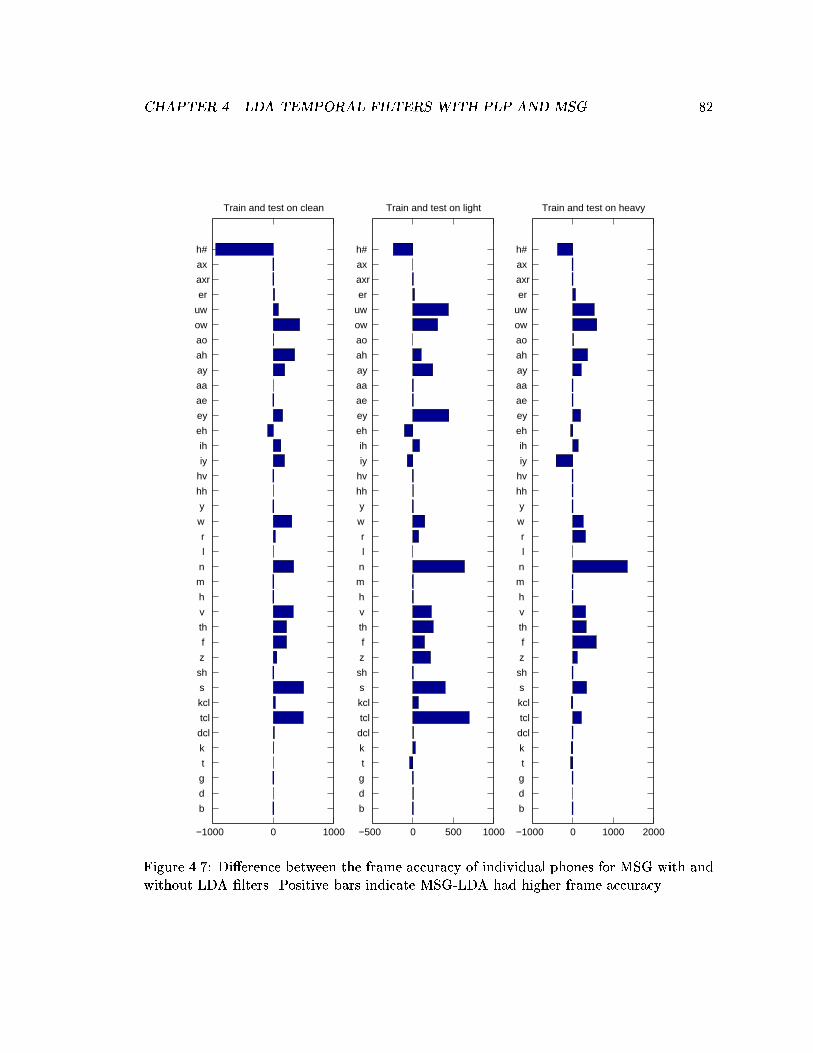
CHAPTER 4. LDA TEMPORAL FILTERS WITH PLP AND MSG 82
−1000 0 1000
b
d
g
t
k
dcl
tcl
kcl
s
sh
z
f
th
v
h
m
n
l
r
w
y
hh
hv
iy
ih
eh
ey
ae
aa
ay
ah
ao
ow
uw
er
axr
ax
h#
Train and test on clean
−500 0 500 1000
b
d
g
t
k
dcl
tcl
kcl
s
sh
z
f
th
v
h
m
n
l
r
w
y
hh
hv
iy
ih
eh
ey
ae
aa
ay
ah
ao
ow
uw
er
axr
ax
h#
Train and test on light
−1000 0 1000 2000
b
d
g
t
k
dcl
tcl
kcl
s
sh
z
f
th
v
h
m
n
l
r
w
y
hh
hv
iy
ih
eh
ey
ae
aa
ay
ah
ao
ow
uw
er
axr
ax
h#
Train and test on heavy
Figure 4.7: Di�erence between the frame accuracy of individual phones for MSG with andwithout LDA �lters. Positive bars indicate MSG-LDA had higher frame accuracy.
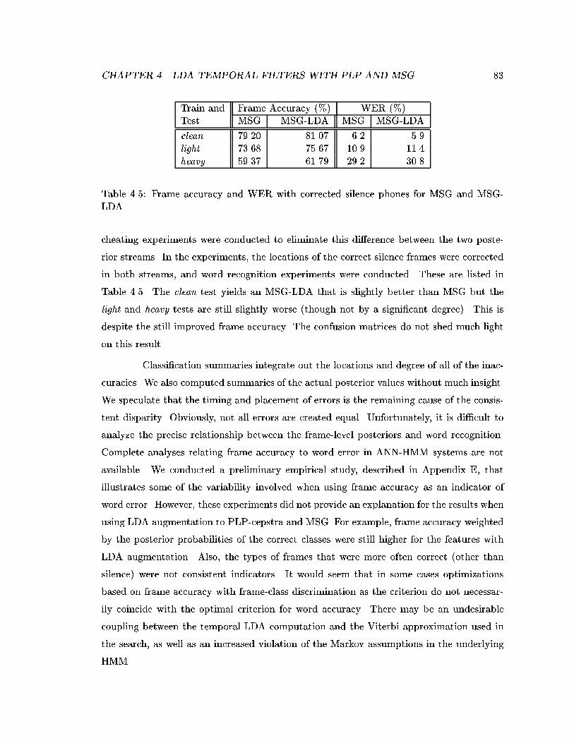
CHAPTER 4. LDA TEMPORAL FILTERS WITH PLP AND MSG 83
Train and Frame Accuracy (%) WER (%)Test MSG MSG-LDA MSG MSG-LDA
clean 79.20 81.07 6.2 5.9light 73.68 75.67 10.9 11.4heavy 59.37 61.79 29.2 30.8
Table 4.5: Frame accuracy and WER with corrected silence phones for MSG and MSG-LDA.
cheating experiments were conducted to eliminate this di�erence between the two poste-
rior streams. In the experiments, the locations of the correct silence frames were corrected
in both streams, and word recognition experiments were conducted. These are listed in
Table 4.5. The clean test yields an MSG-LDA that is slightly better than MSG but the
light and heavy tests are still slightly worse (though not by a signi�cant degree). This is
despite the still improved frame accuracy. The confusion matrices do not shed much light
on this result.
Classi�cation summaries integrate out the locations and degree of all of the inac-
curacies. We also computed summaries of the actual posterior values without much insight.
We speculate that the timing and placement of errors is the remaining cause of the consis-
tent disparity. Obviously, not all errors are created equal. Unfortunately, it is di�cult to
analyze the precise relationship between the frame-level posteriors and word recognition.
Complete analyses relating frame accuracy to word error in ANN-HMM systems are not
available. We conducted a preliminary empirical study, described in Appendix E, that
illustrates some of the variability involved when using frame accuracy as an indicator of
word error. However, these experiments did not provide an explanation for the results when
using LDA augmentation to PLP-cepstra and MSG. For example, frame accuracy weighted
by the posterior probabilities of the correct classes were still higher for the features with
LDA augmentation. Also, the types of frames that were more often correct (other than
silence) were not consistent indicators. It would seem that in some cases optimizations
based on frame accuracy with frame-class discrimination as the criterion do not necessar-
ily coincide with the optimal criterion for word accuracy. There may be an undesirable
coupling between the temporal LDA computation and the Viterbi approximation used in
the search, as well as an increased violation of the Markov assumptions in the underlying
HMM.
CHAPTER 4. LDA TEMPORAL FILTERS WITH PLP AND MSG 84
Fortunately, the LDA augmentation gives a rather consistent improvement in
frame accuracy that can be exploited for some tasks. Di�erent components and methodolo-
gies are often better suited for di�erent tasks. RASTA-PLP and MSG, for example, handle
di�erent situations better. Lieb and Haeb-Umbach found that reverberation-trained LDA
�lters aided MFCCs in TIMIT3 word recognition tests [71] just as we found that it aided
RASTA-PLP in our Numbers tests. Frame-level LDA �lter design presents a useful tool
that can enhance performance in appropriate circumstances.
3A corpus of phonetically balanced sentences spoken by multiple male and female speakers.
85
Chapter 5
Multi-Stream Recognition Tests
One of the e�ects of a change in environmental noise is a change in the feature
distribution. In order to maintain recognition performance the system must either be
retrained or adapt the acoustic models to the new environment. As a complementary
alternative to adaptation we investigated the option of keeping multiple system components
that are trained on data in a sample of environments. Such a system will be able to partially
compensate for the e�ects of a small set of environments. In principle, given appropriate
measures of the noise characteristics, we can select the component that best matches the
training condition. Hopefully, the components can also compensate one another when there
is no match with any of the training conditions and a kind of interpolation between the
the individual components can result.
The previous chapters demonstrated the detrimental e�ects that reverberation
can have on recognition performance. When the system was trained on clean data, the
presence of reverberation degraded the recognition from ca. 5% word error to as much as
ca. 70%. A system trained on highly reverberated data improved such performance to
ca. 30%. Unfortunately, the system had a severely degraded performance on clean data
( degrading from 5% to ca. 30% error). Keeping two systems trained in separate envi-
ronments and intelligently combined should be able to increase the range of robustness to
environments that are similar or have characteristics that lie near either of the trained en-
vironments. Since reverberation presented a very di�cult challenge with very discouraging
word recognition scores, this chapter presents tests using the reverberant environments.
Advantages in combining systems should be more apparent given the di�culty of the task.
CHAPTER 5. MULTI-STREAM RECOGNITION TESTS 86
The experiments used simple combinations of discriminatively trained probability streams
from the previous chapters.
5.1 Simple Combination Strategies
Often when testing a new processing strategy, researchers have discovered that
system performance is enhanced when used in combination with a mature and developed
existing system. One example is using a probability stream derived from MSG features in
combination with a probability stream derived from RASTA-PLP features [62, 60]. Re-
searchers have experimented with numerous means of combining the results of two di�erent
feature processes. In summary, the feature processes may be combined at the feature level,
the frame level, the HMM decoding level, and the recognition output level.
� At the feature level the feature vectors from both processes are concatenated and
treated as a single feature stream from which probabilities are estimated. Feature
selection algorithms (using, for example, component analysis) can be employed to
mitigate the increase in dimensionality.
� At the frame level probabilities are computed for each feature process and the result-
ing probabilities are merged into a single stream prior to decoding. Alternatively,
stacked or cascaded classi�ers such as in a mixture of experts or boosting con�gura-
tion (e.g. [56, 108]) can partition the probability estimation among several classi�ers.
� At the HMM decoding level probabilities are obtained from each stream but the
merging occurs within the HMM decoding. One example of this is HMM recombina-
tion, explored in multi-band systems [10, 11]. In this scheme, pronunciation models
are expanded to include models that re ect the state of both streams. Another possi-
bility is to use a two-pass recognition system [90]. In the �rst pass, word lattices are
computed for each stream that are then combined prior to the second Viterbi search
pass.
� Last, there is combination at the recognition output level. A full word or utterance
recognition is performed on each stream generating sets of NBEST lists [95]. NBEST
is a means of generating a ranked list of the most likely utterances. These NBEST lists
CHAPTER 5. MULTI-STREAM RECOGNITION TESTS 87
can be then be merged into a single NBEST list with the rankings modi�ed using the
utterance scores from both streams. Another method using a voting scheme among
the recognized outputs of several ASR systems is the ROVER system [31].
Many other combination possibilities also exist. Extensive work has been con-
ducted by researchers on using ensembles of classi�ers. Many of the techniques explored
involve classi�cation decision rules from multiple knowledge sources. Soft decision versions
of many of these can be used in statistical ASR systems. Since this work concentrates
on the ASR front-end stage, we only explore those strategies involving combinations at
the feature and frame levels. Our experiments will principally involve simple combinations
of the posterior probabilities that have been employed by other researchers. These com-
bination strategies are justi�ed loosely on varying assumptions. Letting xi represent the
features from stream i and letting q represent classes of set C, some example combinations
are listed here.
Trained probability estimation. P (qjx1; x2; � � � ; xn) is directly estimated from a con-
catenation of feature vectors from all streams with xi being the feature vectors from
each of N streams. An MLP with an appropriate number of parameters is trained
with \one-hot" class targets on the concatenated feature vector. A variant of this is
to train P (qjx1; x2; � � � ; xn) on the posterior probabilities P (qjxi) of each stream or
a related quantity, such as the linear outputs of an MLP that has been trained with
these probabilities.
Conditional independence assumption. In this method, P (qjxi) for each stream is
available and the combined posterior P (qjx1; x2; � � � ; xN ) is estimated from these as
P (qjx1; x2; � � � ; xN ) =P (x1; x2; � � � ; xN jq)p(q)P
q02C P (x1; x2; � � � ; xN jq0)P (q0)(5.1)
=
QNi=1 P (xijq)p(q)P
q02CQNk=1 P (xkjq0)P (q0)
(5.2)
=
QNi=1 P (qjxi) P (xi)P (q)N
P (q)Pq02C
QNk=1 P (q
0jxk) P (xk)P (q0)N
P (q0)(5.3)
=
QNi=1 P (qjxi)=P (q)N�1P
q02CQNk=1 P (q
0jxk)=P (q0)N�1 (5.4)
Equation 5.1 is the application of Bayes rule. In equation 5.2, the features xi are
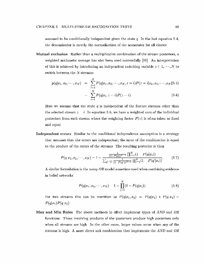
CHAPTER 5. MULTI-STREAM RECOGNITION TESTS 88
assumed to be conditionally independent given the state q. In the last equation 5.4,
the denominator is merely the normalization of the numerator for all classes.
Mutual exclusion. Rather than a multiplicative combination of the stream posteriors, a
weighted arithmetic average has also been used successfully [66]. An interpretation
of this is achieved by introducing an independent switching variable z 2 1; � � � ; N to
switch between the N streams:
p(qjx1; x2; � � � ; xN ) =NXi=1
P (qjx1; x2; � � � ; xN ; z = i)P (z = ijx1; x2; � � � ; xN )(5.5)
=NXi=1
P (qjxi; z = i)P (z = i) (5.6)
Here we assume that the state q is independent of the feature streams other than
the selected stream z = i. In equation 5.6, we have a weighted sum of the individual
posteriors from each stream where the weighting factor P (z) is often taken as �xed
and equal.
Independent errors. Similar to the conditional independence assumption is a strategy
that assumes that the errors are independent; the error of the combination is equal
to the product of the errors of the streams. The resulting posterior is then
P (qjx1; x2; � � � ; xN ) = 1�1
(1�P (q))N�1
QNi=1(1� P (qjxi))P
q02C1
(1�P (q0))N�1
QNi=1(1� P (q0jxi))
: (5.7)
A similar formulation is the noisy-ORmodel sometime used when combining evidence
in belief networks.
P (qjx1; x2; � � � ; xN ) = 1�NYi=1
(1� P (qjxi)) (5.8)
For two streams this can be rewritten as P (qjx1; x2) = P (qjx1) + P (qjx2) �P (qjx1)P (qjx2).
Max and Min Rules. The above methods in e�ect implement types of AND and OR
functions. Those involving products of the posteriors produce high posteriors only
when all streams are high. In the other cases, larger values occur when any of the
streams is high. A more direct soft combination that implements the AND and OR
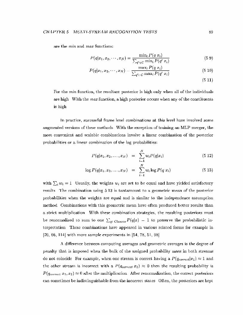
CHAPTER 5. MULTI-STREAM RECOGNITION TESTS 89
are the min and max functions:
P (qjx1; x2; � � � ; xN ) = mini P (qjxi)Pq02C mini P (q0jxi) (5.9)
P (qjx1; x2; � � � ; xN ) = maxi P (qjxi)Pq02C maxi P (q0jxi)
(5.10)
(5.11)
For the min function, the resultant posterior is high only when all of the individuals
are high. With the max function, a high posterior occurs when any of the constituents
is high.
In practice, successful frame level combinations at this level have involved some
augmented versions of these methods. With the exception of training an MLP merger, the
most convenient and scalable combinations involve a linear combination of the posterior
probabilities or a linear combination of the log probabilities:
P (qjx1; x2; : : : ; xN ) =NXi=1
wiP (qjxi) (5.12)
log P (qjx1; x2; : : : ; xN ) =NXi=1
wi log P (qjxi) (5.13)
withP
i wi = 1. Usually, the weights wi are set to be equal and have yielded satisfactory
results. The combination using 5.13 is tantamount to a geometric mean of the posterior
probabilities when the weights are equal and is similar to the independence assumption
method. Combinations with this geometric mean have often produced better results than
a strict multiplication. With these combination strategies, the resulting posteriors must
be renormalized to sum to oneP
q2Classes P (qjx) = 1 to preserve the probabilistic in-
terpretation. These combinations have appeared in various related forms for example in
[70, 66, 114] with more sample experiments in [54, 78, 51, 98].
A di�erence between computing averages and geometric averages is the degree of
penalty that is imposed when the bulk of the assigned probability mass in both streams
do not coincide. For example, when one stream is correct having a P (qcorrectjx1) � 1 and
the other stream is incorrect with a P (qcorrectjx2) � 0 then the resulting probability is
P (qcorrectjx1; x2) � 0 after the multiplication. After renormalization, the correct posteriors
can sometimes be indistinguishable from the incorrect states. Often, the posteriors are kept
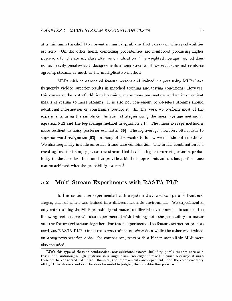
CHAPTER 5. MULTI-STREAM RECOGNITION TESTS 90
at a minimum threshold to prevent numerical problems that can occur when probabilities
are zero. On the other hand, coinciding probabilities are reinforced producing higher
posteriors for the correct class after renormalization. The weighted average method does
not as heavily penalize such disagreements among streams. However, it does not reinforce
agreeing streams as much as the multiplicative method.
MLPs with concatenated feature vectors and trained mergers using MLPs have
frequently yielded superior results in matched training and testing conditions. However,
this comes at the cost of additional training, many more parameters, and an inconvenient
means of scaling to more streams. It is also not convenient to de-select streams should
additional information or constraints require it. In this work we perform most of the
experiments using the simple combination strategies using the linear average method in
equation 5.12 and the log-average method in equation 5.13. The linear average method is
more resilient to noisy posterior estimates [66]. The log-average, however, often leads to
superior word recognition [63]. In many of the results to follow we include both methods.
We also frequently include an oracle frame-wise combination. The oracle combination is a
cheating test that simply passes the stream that has the highest correct posterior proba-
bility to the decoder. It is used to provide a kind of upper limit as to what performance
can be achieved with the probability streams1.
5.2 Multi-Stream Experiments with RASTA-PLP
In this section, we experimented with a system that used two parallel front-end
stages, each of which was trained in a di�erent acoustic environment. We experimented
only with training the MLP probability estimator to di�erent environments. In some of the
following sections, we will also experimented with training both the probability estimator
and the feature extraction together. For these experiments, the feature extraction process
used was RASTA-PLP. One stream was trained on clean data while the other was trained
on heavy reverberation data. For comparison, tests with a bigger monolithic MLP were
also included.
1With this type of cheating combination, any additional stream, including purely random ones or atrivial one containing a high posterior in a single class, can only improve the frame accuracy; it musttherefore be considered with care. However, the improvements are dependent upon the complementaryutility of the streams and can therefore be useful in judging their combination potential.
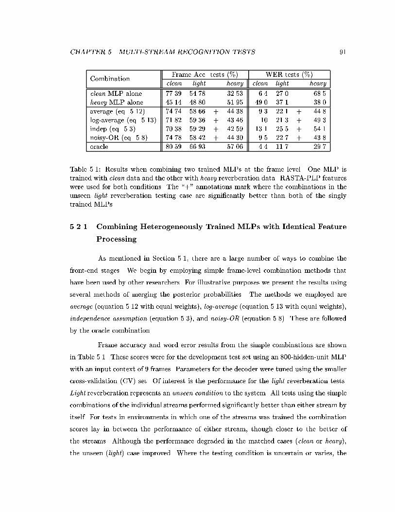
CHAPTER 5. MULTI-STREAM RECOGNITION TESTS 91
Frame Acc. tests (%) WER tests (%)Combination
clean light heavy clean light heavy
clean MLP alone 77.39 54.78 32.53 6.4 27.0 68.5heavy MLP alone 45.14 48.80 51.95 49.0 37.1 38.0
average (eq. 5.12) 74.74 58.66 + 44.38 9.3 22.1 + 44.8log-average (eq. 5.13) 71.82 59.36 + 43.46 10 21.3 + 49.3indep (eq. 5.3) 70.38 59.29 + 42.59 13.1 25.5 + 54.1noisy-OR (eq. 5.8) 74.78 58.42 + 44.30 9.5 22.7 + 43.8
oracle 80.59 66.93 57.06 4.4 11.7 29.7
Table 5.1: Results when combining two trained MLPs at the frame level. One MLP istrained with clean data and the other with heavy reverberation data. RASTA-PLP featureswere used for both conditions. The \+" annotations mark where the combinations in theunseen light reverberation testing case are signi�cantly better than both of the singlytrained MLPs.
5.2.1 Combining Heterogeneously Trained MLPs with Identical Feature
Processing
As mentioned in Section 5.1, there are a large number of ways to combine the
front-end stages. We begin by employing simple frame-level combination methods that
have been used by other researchers. For illustrative purposes we present the results using
several methods of merging the posterior probabilities. The methods we employed are
average (equation 5.12 with equal weights), log-average (equation 5.13 with equal weights),
independence assumption (equation 5.3), and noisy-OR (equation 5.8). These are followed
by the oracle combination.
Frame accuracy and word error results from the simple combinations are shown
in Table 5.1. These scores were for the development test set using an 800-hidden-unit MLP
with an input context of 9 frames. Parameters for the decoder were tuned using the smaller
cross-validation (CV) set. Of interest is the performance for the light reverberation tests.
Light reverberation represents an unseen condition to the system. All tests using the simple
combinations of the individual streams performed signi�cantly better than either stream by
itself. For tests in environments in which one of the streams was trained the combination
scores lay in between the performance of either stream, though closer to the better of
the streams. Although the performance degraded in the matched cases (clean or heavy),
the unseen (light) case improved. Where the testing condition is uncertain or varies, the
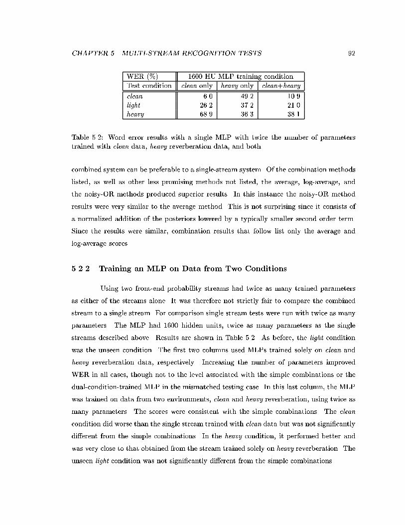
CHAPTER 5. MULTI-STREAM RECOGNITION TESTS 92
WER (%) 1600 HU MLP training condition
Test condition clean only heavy only clean+heavy
clean 6.0 49.2 10.9light 26.2 37.2 21.0heavy 68.9 36.3 38.1
Table 5.2: Word error results with a single MLP with twice the number of parameterstrained with clean data, heavy reverberation data, and both.
combined system can be preferable to a single-stream system. Of the combination methods
listed, as well as other less promising methods not listed, the average, log-average, and
the noisy-OR methods produced superior results. In this instance the noisy-OR method
results were very similar to the average method. This is not surprising since it consists of
a normalized addition of the posteriors lowered by a typically smaller second order term.
Since the results were similar, combination results that follow list only the average and
log-average scores.
5.2.2 Training an MLP on Data from Two Conditions
Using two front-end probability streams had twice as many trained parameters
as either of the streams alone. It was therefore not strictly fair to compare the combined
stream to a single stream. For comparison single stream tests were run with twice as many
parameters. The MLP had 1600 hidden units, twice as many parameters as the single
streams described above. Results are shown in Table 5.2. As before, the light condition
was the unseen condition. The �rst two columns used MLPs trained solely on clean and
heavy reverberation data, respectively. Increasing the number of parameters improved
WER in all cases, though not to the level associated with the simple combinations or the
dual-condition-trained MLP in the mismatched testing case. In this last column, the MLP
was trained on data from two environments, clean and heavy reverberation, using twice as
many parameters. The scores were consistent with the simple combinations. The clean
condition did worse than the single stream trained with clean data but was not signi�cantly
di�erent from the simple combinations. In the heavy condition, it performed better and
was very close to that obtained from the stream trained solely on heavy reverberation. The
unseen light condition was not signi�cantly di�erent from the simple combinations.
CHAPTER 5. MULTI-STREAM RECOGNITION TESTS 93
Simply increasing the number of parameters for the trained MLP improved recog-
nition scores. However, the condition of the data used to train the MLP seemed crucial
to achieving robustness to varying environments. For example, merely adding parameters
to the clean-trained MLP did not yield scores for the heavy reverberation that were on
par with a heavy-trained system. For the unseen light condition, good performance may
eventually be achieved but not at the rate associated with adding some heavy reverberation
training data. Training a large single net with multiple environments produced results that
were at least as good as the simple combinations, though sometimes better. The interpola-
tion power of the MLP was su�cient to handle the light case as a compromise between the
two extreme training conditions. There are disadvantages with this approach compared to
the simple combination strategy. Training large MLPs is less convenient due to training
time and the fact that it must be completely retrained with every new environment we wish
to add or subtract. The smaller environment-speci�c streams may be trained separately
and in parallel. The simple frame-level multi-stream architecture also makes it possible
and convenient to de-select streams or add streams if additional information about the
environment is available. A monolithic MLP is not easily adapted in this way and becomes
computationally expensive when we wish to train on more than two environments. These
issues also arise if we consider a trained MLP as a stream merger.
Whether using a monolithic MLP or a trained MLP merger the feature streams
are merged in a non-linear fashion. This is a more powerful method than the simple
combination strategies and therefore has typically resulted in superior performance in tests
by many researchers, for example by Sharma [100]. Trained MLPs, however, still represent
a rather static means of combination. Architectural changes or extra inputs can be used
to provide a more dynamic combination means that may also allow stream de-emphasis.
However, we continue to use the simple combination strategies for convenience: no need
for additional training data, dynamic weighting schemes are readily implementable, and
simple combination results are still indicative of performance advantage.
5.3 RASTA-PLP with Di�erent LDA Filters
We observed in Chapter 3 that di�erent acoustic environments resulted in tem-
poral �lters with di�erent frequency ranges. When using an MLP lacking acoustic context,
CHAPTER 5. MULTI-STREAM RECOGNITION TESTS 94
such �lters o�ered some advantages in di�erent acoustic environments. A further exami-
nation of the frame errors indicated certain di�erences in the recognized frames that could
potentially be exploited. In this section we tested multi-stream combinations using LDA-
RASTA-PLP with �lters trained in di�erent environments.
5.3.1 Dual LDA Filter Sets with Common MLP Training Environment
In this experiment we ascertained if improvements could be gained when using
streams from two identical feature processes, LDA-RASTA-PLP, with only a di�erence in
the frequency responses of the RASTA �lters. For these tests, we used probability streams
from two heterogeneously trained front-end temporal �lters. The �rst stream used the LDA
�lters derived from the clean condition and whose principal component had an average
band-pass response of 1 to 13 Hz. The second stream used the LDA �lters derived from
the highly reverberant condition and whose principal component had a narrower average
band-pass response of 1 to 5 Hz. Since the �lter sets preserved di�erent modulation rates,
this combination of feature processing was e�ectively a multi-rate front-end combination.
The MLP probability estimator for both streams was trained on the the same environment
as the LDA �lters, though using data from the Numbers corpus rather than from the
Stories corpus. We initially allowed the MLP access to only a single frame of acoustic
features in order to eliminate the possibility of redundant temporal processing that an
acoustic context would provide.
Single Frame Acoustic Context
Tables 5.3, 5.4 and 5.5 contain the results where the MLP probability estimators
for both streams were trained on clean, light reverberation, and heavy reverberation data
respectively. The �rst two rows of the table pertain to the word error recognition results for
the streams taken individually. The following two rows contain word error when the frame-
level posterior probabilities were averaged prior to the decoding and where the logarithm of
the posteriors were averaged. The last row contains the WER from an oracle combination
of the two streams.
We see from these results that these simple combinations of the two front ends
with only a di�erence in the temporal characteristics of the �lters improved the performance

CHAPTER 5. MULTI-STREAM RECOGNITION TESTS 95
Clean trained MLP WER (%)Combination clean test light test heavy test
clean LDA �lter alone 9.1 33.1 72.5heavy LDA �lter alone 12.0 30.2 73.4
average 8.8 28.5 + 69.7 +log-average 8.9 27.9 + 69.1 +
oracle 4.8 16.8 60.8
Table 5.3: WER Results from a frame-level combination of LDA-RASTA-PLP with LDA�lters derived under clean and heavy reverberation conditions. The MLP probability es-timator was trained with clean data and a single frame of acoustic features. The \+"annotations mark where the combinations are better than the single streams.
Light trained MLP WER (%)Combination clean test light test heavy test
clean LDA �lter alone 16.9 18.9 62.6heavy LDA �lter alone 20.1 18.3 63.5
average 14.6 + 16.7 + 60.0 +log-average 13.8 + 16.3 + 60.3 +
oracle 7.70 10.10 50.2
Table 5.4: WER Results from a frame-level combination of LDA-RASTA-PLP with LDA�lters derived under clean and heavy reverberation conditions. The MLP probability esti-mator was trained with light reverberation data and a single frame of acoustic features.The \+" annotations mark where the combinations are better than the single streams.
Heavy trained MLP WER (%)Combination clean test light test heavy test
clean LDA �lter alone 47.0 42.7 45.5heavy LDA �lter alone 43.2 37.8 38.9
average 39.0 + 35.5 + 39.3log-average 38.3 + 34.8 + 38.8
oracle 26.9 23.8 29.70
Table 5.5: WER Results from a frame-level combination of LDA-RASTA-PLP with LDA�lters derived under clean and heavy heavy reverberation conditions. The MLP probabilityestimator was trained with heavy reverberation data and a single frame of acousticfeatures. The \+" annotations mark where the combinations are better than the singlestreams.
CHAPTER 5. MULTI-STREAM RECOGNITION TESTS 96
over either stream individually. This improvement occurred consistently in tests where the
testing condition di�ered from the condition on which the MLP was trained. We see that
with most improvements occuring in mismatched cases, using a combination of �lters with
di�erent ranges aids in robustness in this case. In matched testing conditions, the results
were not very di�erent from those of the individual streams. The exception to this is
where the MLPs were trained on light reverberation data, though in these instances the
LDA �lters that were optimized for the light condition were not used. Referring to Table
3.10 in Chapter 3, the combination of the clean and heavy �lters with an MLP trained with
light reverberation data yielded results that were equivalent (light test) or superior (clean
and heavy tests) to the result where both the MLP and the LDA �lters were trained on
the light reverberation data. As mentioned previously, a direct comparison is not strictly
fair given the di�erence in the number of parameters, though previous tests indicate that
a further fair test with equal numbers of parameters would yield similar results.
9 Frame Acoustic Context
We noted in Section 3.3.3 that allowing the MLP probability estimator a context
of acoustic features mitigated much of the performance di�erences when using separate
LDA �lters tuned to the matching acoustic condition. Since the �lters derived under heavy
reverberation had more selective frequency responses we observed that there were some
di�erences in frame classi�cation that might be exploited by using a combination. For
example, the second stream using the more constrained �lter may be used to reinforce
those frames that were correct. We therefore repeated the experiments with MLPs that
were allowed an acoustic context of approximately 100 ms. These results are shown in
Tables 5.6, 5.7, and 5.8 for MLPs that were trained under clean, light reverberation, and
heavy reverberation, respectively. We see from these scores that the simple combinations
performed as well as or better than either stream alone, though signi�cant improvements
occurred in fewer test cases.
5.3.2 Matched LDA Filter and MLP Training Environments
In these tests we see if the enhancements a�orded by LDA �lters with RASTA-
PLP also carry over to multi-stream tests with heterogeneous stream training environments.
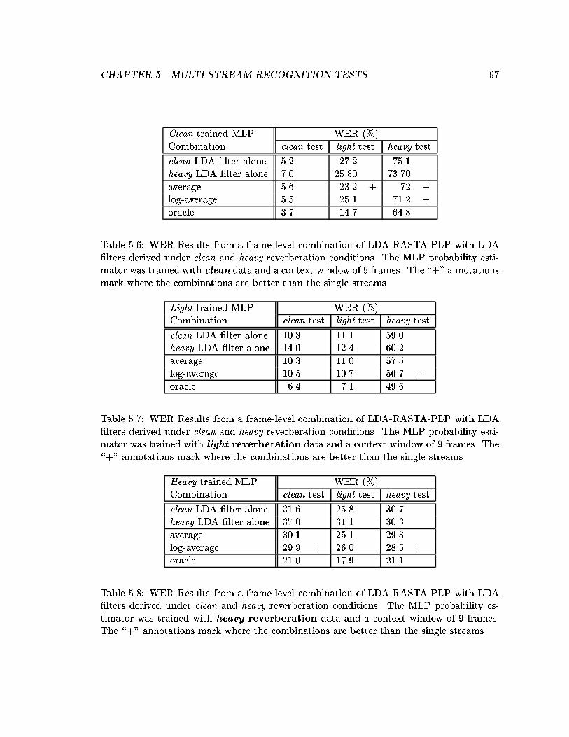
CHAPTER 5. MULTI-STREAM RECOGNITION TESTS 97
Clean trained MLP WER (%)Combination clean test light test heavy test
clean LDA �lter alone 5.2 27.2 75.1heavy LDA �lter alone 7.0 25.80 73.70
average 5.6 23.2 + 72 +log-average 5.5 25.1 71.2 +
oracle 3.7 14.7 64.8
Table 5.6: WER Results from a frame-level combination of LDA-RASTA-PLP with LDA�lters derived under clean and heavy reverberation conditions. The MLP probability esti-mator was trained with clean data and a context window of 9 frames. The \+" annotationsmark where the combinations are better than the single streams.
Light trained MLP WER (%)Combination clean test light test heavy test
clean LDA �lter alone 10.8 11.1 59.0heavy LDA �lter alone 14.0 12.4 60.2
average 10.3 11.0 57.5log-average 10.5 10.7 56.7 +
oracle 6.4 7.1 49.6
Table 5.7: WER Results from a frame-level combination of LDA-RASTA-PLP with LDA�lters derived under clean and heavy reverberation conditions. The MLP probability esti-mator was trained with light reverberation data and a context window of 9 frames. The\+" annotations mark where the combinations are better than the single streams.
Heavy trained MLP WER (%)Combination clean test light test heavy test
clean LDA �lter alone 31.6 25.8 30.7heavy LDA �lter alone 37.0 31.1 30.3
average 30.1 25.1 29.3log-average 29.9 + 26.0 28.5 +
oracle 21.0 17.9 21.1
Table 5.8: WER Results from a frame-level combination of LDA-RASTA-PLP with LDA�lters derived under clean and heavy reverberation conditions. The MLP probability es-timator was trained with heavy reverberation data and a context window of 9 frames.The \+" annotations mark where the combinations are better than the single streams.
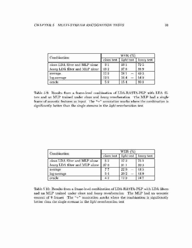
CHAPTER 5. MULTI-STREAM RECOGNITION TESTS 98
WER (%)Combination
clean test light test heavy test
clean LDA �lter and MLP alone 9.1 33.1 72.5heavy LDA �lter and MLP alone 43.2 37.8 38.9
average 12.9 28.1 + 49.3log-average 13.5 26.4 + 54.0
oracle 5.9 15.4 30.1
Table 5.9: Results from a frame-level combination of LDA-RASTA-PLP with LDA �l-ters and an MLP trained under clean and heavy reverberation. The MLP had a singleframe of acoustic features as input. The \+" annotation marks where the combination issigni�cantly better than the single streams in the light reverberation test.
WER (%)Combination
clean test light test heavy test
clean LDA �lter and MLP alone 5.2 27.2 75.1heavy LDA �lter and MLP alone 37.0 31.1 30.3
average 7.7 22.0 + 44.5log-average 9.4 20.2 + 44.9
oracle 4.2 12.9 24.7
Table 5.10: Results from a frame-level combination of LDA-RASTA-PLP with LDA �ltersand an MLP trained under clean and heavy reverberation. The MLP had an acousticcontext of 9 frames. The \+" annotation marks where the combination is signi�cantlybetter than the single streams in the light reverberation test.
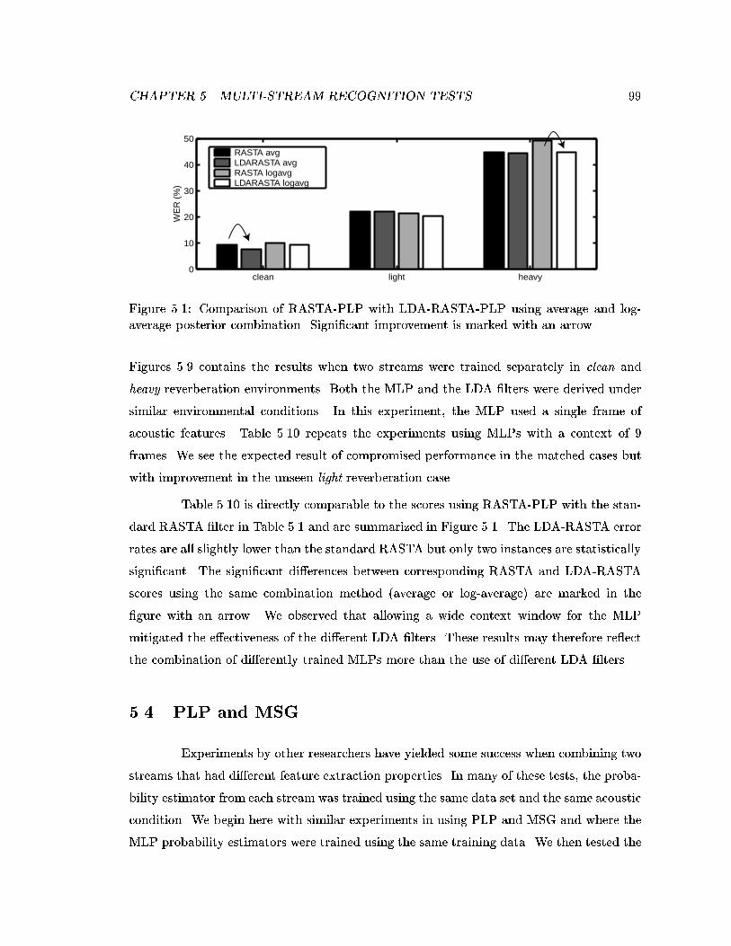
CHAPTER 5. MULTI-STREAM RECOGNITION TESTS 99
clean light heavy0
10
20
30
40
50
WE
R (
%)
RASTA avg LDARASTA avg RASTA logavg LDARASTA logavg
Figure 5.1: Comparison of RASTA-PLP with LDA-RASTA-PLP using average and log-average posterior combination. Signi�cant improvement is marked with an arrow.
Figures 5.9 contains the results when two streams were trained separately in clean and
heavy reverberation environments. Both the MLP and the LDA �lters were derived under
similar environmental conditions. In this experiment, the MLP used a single frame of
acoustic features. Table 5.10 repeats the experiments using MLPs with a context of 9
frames. We see the expected result of compromised performance in the matched cases but
with improvement in the unseen light reverberation case.
Table 5.10 is directly comparable to the scores using RASTA-PLP with the stan-
dard RASTA �lter in Table 5.1 and are summarized in Figure 5.1. The LDA-RASTA error
rates are all slightly lower than the standard RASTA but only two instances are statistically
signi�cant. The signi�cant di�erences between corresponding RASTA and LDA-RASTA
scores using the same combination method (average or log-average) are marked in the
�gure with an arrow. We observed that allowing a wide context window for the MLP
mitigated the e�ectiveness of the di�erent LDA �lters. These results may therefore re ect
the combination of di�erently trained MLPs more than the use of di�erent LDA �lters.
5.4 PLP and MSG
Experiments by other researchers have yielded some success when combining two
streams that had di�erent feature extraction properties. In many of these tests, the proba-
bility estimator from each stream was trained using the same data set and the same acoustic
condition. We begin here with similar experiments in using PLP and MSG and where the
MLP probability estimators were trained using the same training data. We then tested the
CHAPTER 5. MULTI-STREAM RECOGNITION TESTS 100
combined probability streams trained in heterogeneous reverberant environments.
5.4.1 Dual-stream PLP and MSG with Common MLP Training Envi-
ronment
In the previous LDA-RASTA-PLP tests the feature-extraction processes for the
di�erent streams were identical except for the frequency selectivity of the temporal �lters.
Here we experimented with feature extraction processes that were much more distinct.
Previous work by Wu and Kingsbury have demonstrated some advantage in using PLP
and MSG in combination [60, 119]. Though PLP and MSG contain processing elements
that are similar in function, they are computed in alternative ways that have di�erent
properties. These di�erent properties can allow for complementary errors that may be
exploited; the inabilities of one stream may be compensated for by the other stream. We
replicated the experiments performed in previous sections using simple combinations of
MLPs trained under the same acoustic environment to provide a baseline.
Tables 5.11, 5.12, and 5.13 contain simple combination results. The simple combi-
nations improved the word error signi�cantly in most cases. The combination score using
the clean MLPs and clean test was the best score (to our knowledge) achieved on this
task. Furthermore, the oracle combination in that case was close to the lowest possible
word error2. Just as the PLP and MSG features with normalization performed better than
RASTA-PLP on this task, the combinations were also better. The scores were on par or
better than the oracle cheating combination using RASTA-PLP and were superior to the
WER scores from average and log-average combinations.
5.4.2 PLP and MSG with Heterogeneously Trained MLPs
We repeated the experiments using two streams wherein the MLPs were trained
separately on clean and heavy reverberation. Since PLP had the lowest word error on clean
tests, we used an MLP trained on clean data with PLP. Similarly, MSG had the lowest
word error scores on reverberation tests and we therefore used an MLP trained on heavy
reverberation with MSG. The results of this pairing are shown in Table 5.14. Again, light
reverberation was the unseen condition.
2Decoding completely accurate frame posteriors.
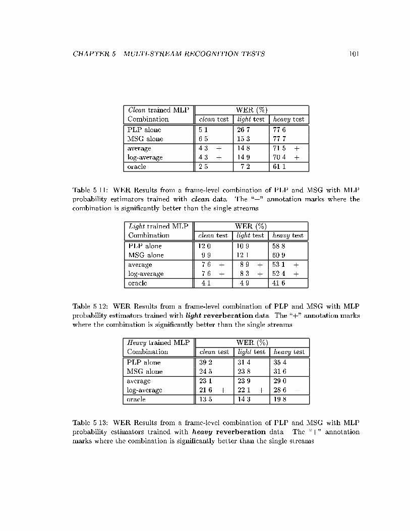
CHAPTER 5. MULTI-STREAM RECOGNITION TESTS 101
Clean trained MLP WER (%)Combination clean test light test heavy test
PLP alone 5.1 26.7 77.6MSG alone 6.5 15.3 77.7
average 4.3 + 14.8 71.5 +log-average 4.3 + 14.9 70.4 +
oracle 2.5 7.2 61.1
Table 5.11: WER Results from a frame-level combination of PLP and MSG with MLPprobability estimators trained with clean data. The \+" annotation marks where thecombination is signi�cantly better than the single streams.
Light trained MLP WER (%)Combination clean test light test heavy test
PLP alone 12.0 10.9 58.8MSG alone 9.9 12.1 60.9
average 7.6 + 8.9 + 53.1 +log-average 7.6 + 8.3 + 52.4 +
oracle 4.1 4.9 41.6
Table 5.12: WER Results from a frame-level combination of PLP and MSG with MLPprobability estimators trained with light reverberation data. The \+" annotation markswhere the combination is signi�cantly better than the single streams.
Heavy trained MLP WER (%)Combination clean test light test heavy test
PLP alone 39.2 31.4 35.4MSG alone 24.5 23.8 31.6
average 23.1 23.9 29.0 +log-average 21.6 + 22.1 + 28.6 +
oracle 13.5 14.3 19.8
Table 5.13: WER Results from a frame-level combination of PLP and MSG with MLPprobability estimators trained with heavy reverberation data. The \+" annotationmarks where the combination is signi�cantly better than the single streams.
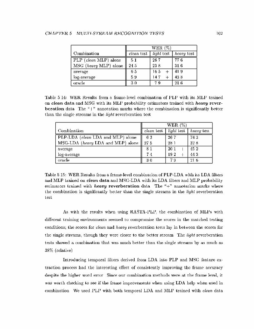
CHAPTER 5. MULTI-STREAM RECOGNITION TESTS 102
WER (%)Combination clean test light test heavy test
PLP (clean MLP) alone 5.1 26.7 77.6MSG (heavy MLP) alone 24.5 23.8 31.6
average 6.5 16.5 + 41.9log-average 5.9 14.7 + 43.8
oracle 3.0 7.9 21.6
Table 5.14: WER Results from a frame-level combination of PLP with its MLP trainedon clean data and MSG with its MLP probability estimators trained with heavy rever-
beration data. The \+" annotation marks where the combination is signi�cantly betterthan the single streams in the light reverberation test.
WER (%)Combination clean test light test heavy test
PLP-LDA (clean LDA and MLP) alone 6.3 26.7 74.3MSG-LDA (heavy LDA and MLP) alone 27.5 28.1 32.8
average 8.1 20.1 + 45.2log-average 7.4 19.2 + 44.3
oracle 3.0 7.9 21.6
Table 5.15: WER Results from a frame-level combination of PLP-LDA with its LDA �ltersand MLP trained on clean data and MSG-LDA with its LDA �lters and MLP probabilityestimators trained with heavy reverberation data. The \+" annotation marks wherethe combination is signi�cantly better than the single streams in the light reverberationtest.
As with the results when using RASTA-PLP, the combination of MLPs with
di�erent training environments seemed to compromise the scores in the matched testing
conditions; the scores for clean and heavy reverberation tests lay in between the scores for
the single streams, though they were closer to the better stream. The light reverberation
tests showed a combination that was much better than the single streams by as much as
38% (relative).
Introducing temporal �lters derived from LDA into PLP and MSG feature ex-
traction process had the interesting e�ect of consistently improving the frame accuracy
despite the higher word error. Since our combination methods were at the frame level, it
was worth checking to see if the frame improvements when using LDA help when used in
combination. We used PLP with both temporal LDA and MLP trained with clean data
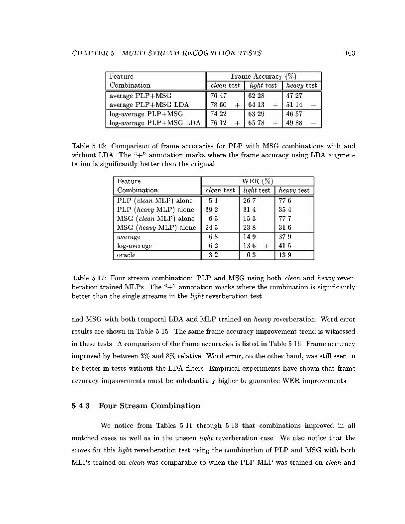
CHAPTER 5. MULTI-STREAM RECOGNITION TESTS 103
Feature Frame Accuracy (%)Combination clean test light test heavy test
average PLP+MSG 76.47 62.28 47.27average PLP+MSG LDA 78.60 + 64.13 + 51.14 +
log-average PLP+MSG 74.22 63.29 46.57log-average PLP+MSG LDA 76.12 + 65.78 + 49.88 +
Table 5.16: Comparison of frame accuracies for PLP with MSG combinations with andwithout LDA. The \+" annotation marks where the frame accuracy using LDA augmen-tation is signi�cantly better than the original.
Feature WER (%)Combination clean test light test heavy test
PLP (clean MLP) alone 5.1 26.7 77.6PLP (heavy MLP) alone 39.2 31.4 35.4MSG (clean MLP) alone 6.5 15.3 77.7MSG (heavy MLP) alone 24.5 23.8 31.6
average 6.8 14.9 37.9log-average 6.2 13.6 + 41.5
oracle 3.2 6.3 13.9
Table 5.17: Four stream combination: PLP and MSG using both clean and heavy rever-beration trained MLPs. The \+" annotation marks where the combination is signi�cantlybetter than the single streams in the light reverberation test.
and MSG with both temporal LDA and MLP trained on heavy reverberation. Word error
results are shown in Table 5.15. The same frame accuracy improvement trend is witnessed
in these tests. A comparison of the frame accuracies is listed in Table 5.16. Frame accuracy
improved by between 3% and 8% relative. Word error, on the other hand, was still seen to
be better in tests without the LDA �lters. Empirical experiments have shown that frame
accuracy improvements must be substantially higher to guarantee WER improvements.
5.4.3 Four Stream Combination
We notice from Tables 5.11 through 5.13 that combinations improved in all
matched cases as well as in the unseen light reverberation case. We also notice that the
scores for this light reverberation test using the combination of PLP and MSG with both
MLPs trained on clean was comparable to when the PLP MLP was trained on clean and
CHAPTER 5. MULTI-STREAM RECOGNITION TESTS 104
the MSG MLP was trained on heavy reverberation. Further improvements may be ob-
tained when using PLP and MSG trained both on clean and heavy reverberation. The
simple combination method allowed us to do this readily. Results for this test are shown
in Table 5.17. The best combination results for the unseen light condition case occurred
using the log-average combination. Most of the remaining scores remained near the two
stream performance.
5.5 Weighted Stream Combinations
So far, combination experiments used averaged posteriors with equal weighting.
In the matched training and testing conditions, the equal weighting resulted in word error
scores in between that of either stream. In such a situation, it is prudent to de-select the
worst of the streams to recover the best score. It is not di�cult to imagine that other
circumstances exist where a non-equal weighting would also be preferable. When explicit
knowledge of the environmental characteristics is available, better performance may be
achieved.
In order to observe the e�ect of environmental characteristics on the choice of
weighting we performed tests using room impulses with di�erent reverberation character-
istics. We performed tests varying relative weighting between two streams, one trained
with clean data and the other on heavy reverberation. We then tested on the reverbera-
tion room impulse responses that were arti�cially modi�ed to yield certain reverberation
characteristics, as done in Section 3.2.2. The room impulse T60 varied between 0.25 and
2.5 seconds in 0.25-second increments while the DTR remained �xed at -8 dB. Additional
tests used a DTR varying between -8 to 2 dB in 1-dB increments while holding the T60
constant at 2 seconds. These tests were performed on the smaller CV set using constant
parameters for the decoder. The log-average combination method worked slightly better
than the arithmetic averaging in the unseen test cases (as these tests can be considered)
and was used here.
LDA-RASTA-PLP
We �rst tested the relative weighting using two LDA-RASTA-PLP streams using
clean and heavy LDA �lters separately for each stream. These streams re ected MLPs
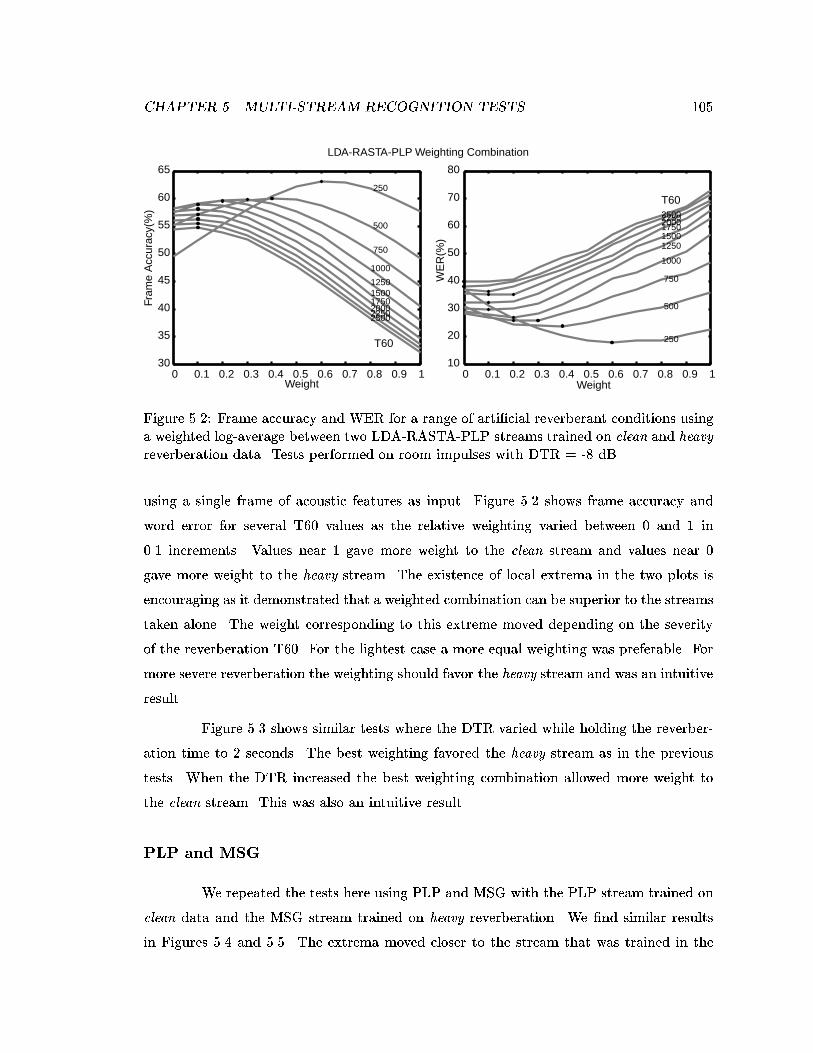
CHAPTER 5. MULTI-STREAM RECOGNITION TESTS 105
0 0.1 0.2 0.3 0.4 0.5 0.6 0.7 0.8 0.9 130
35
40
45
50
55
60
65
250
500
750
1000
125015001750200022502500
T60
Weight
Fram
e A
ccur
acy(
%)
LDA-RASTA-PLP Weighting Combination
0 0.1 0.2 0.3 0.4 0.5 0.6 0.7 0.8 0.9 110
20
30
40
50
60
70
80
250
500
750
1000
125015001750200022502500
T60
Weight
WE
R(%
)
Figure 5.2: Frame accuracy and WER for a range of arti�cial reverberant conditions usinga weighted log-average between two LDA-RASTA-PLP streams trained on clean and heavyreverberation data. Tests performed on room impulses with DTR = -8 dB.
using a single frame of acoustic features as input. Figure 5.2 shows frame accuracy and
word error for several T60 values as the relative weighting varied between 0 and 1 in
0.1 increments. Values near 1 gave more weight to the clean stream and values near 0
gave more weight to the heavy stream. The existence of local extrema in the two plots is
encouraging as it demonstrated that a weighted combination can be superior to the streams
taken alone. The weight corresponding to this extreme moved depending on the severity
of the reverberation T60. For the lightest case a more equal weighting was preferable. For
more severe reverberation the weighting should favor the heavy stream and was an intuitive
result.
Figure 5.3 shows similar tests where the DTR varied while holding the reverber-
ation time to 2 seconds. The best weighting favored the heavy stream as in the previous
tests. When the DTR increased the best weighting combination allowed more weight to
the clean stream. This was also an intuitive result.
PLP and MSG
We repeated the tests here using PLP and MSG with the PLP stream trained on
clean data and the MSG stream trained on heavy reverberation. We �nd similar results
in Figures 5.4 and 5.5. The extrema moved closer to the stream that was trained in the
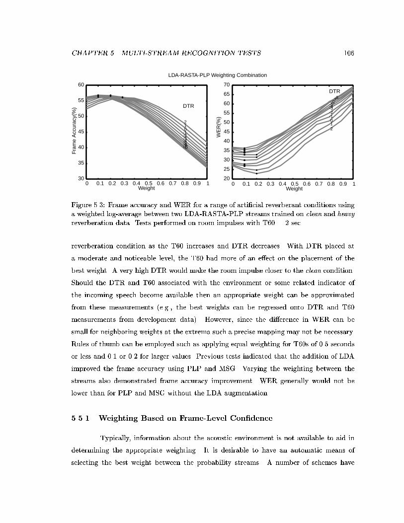
CHAPTER 5. MULTI-STREAM RECOGNITION TESTS 106
0 0.1 0.2 0.3 0.4 0.5 0.6 0.7 0.8 0.9 130
35
40
45
50
55
60
-8-7-6-5-4-3-2-1 0 1 2
DTR
Weight
Fram
e A
ccur
acy(
%)
LDA-RASTA-PLP Weighting Combination
0 0.1 0.2 0.3 0.4 0.5 0.6 0.7 0.8 0.9 120
25
30
35
40
45
50
55
60
65
70
-8-7-6-5-4-3-2-1 0 1 2
DTR
Weight
WE
R(%
)
Figure 5.3: Frame accuracy and WER for a range of arti�cial reverberant conditions usinga weighted log-average between two LDA-RASTA-PLP streams trained on clean and heavyreverberation data. Tests performed on room impulses with T60 = 2 sec.
reverberation condition as the T60 increases and DTR decreases. With DTR placed at
a moderate and noticeable level, the T60 had more of an e�ect on the placement of the
best weight. A very high DTR would make the room impulse closer to the clean condition.
Should the DTR and T60 associated with the environment or some related indicator of
the incoming speech become available then an appropriate weight can be approximated
from these measurements (e.g., the best weights can be regressed onto DTR and T60
measurements from development data). However, since the di�erence in WER can be
small for neighboring weights at the extrema such a precise mapping may not be necessary.
Rules of thumb can be employed such as applying equal weighting for T60s of 0.5 seconds
or less and 0.1 or 0.2 for larger values. Previous tests indicated that the addition of LDA
improved the frame accuracy using PLP and MSG. Varying the weighting between the
streams also demonstrated frame accuracy improvement. WER generally would not be
lower than for PLP and MSG without the LDA augmentation.
5.5.1 Weighting Based on Frame-Level Con�dence
Typically, information about the acoustic environment is not available to aid in
determining the appropriate weighting. It is desirable to have an automatic means of
selecting the best weight between the probability streams. A number of schemes have
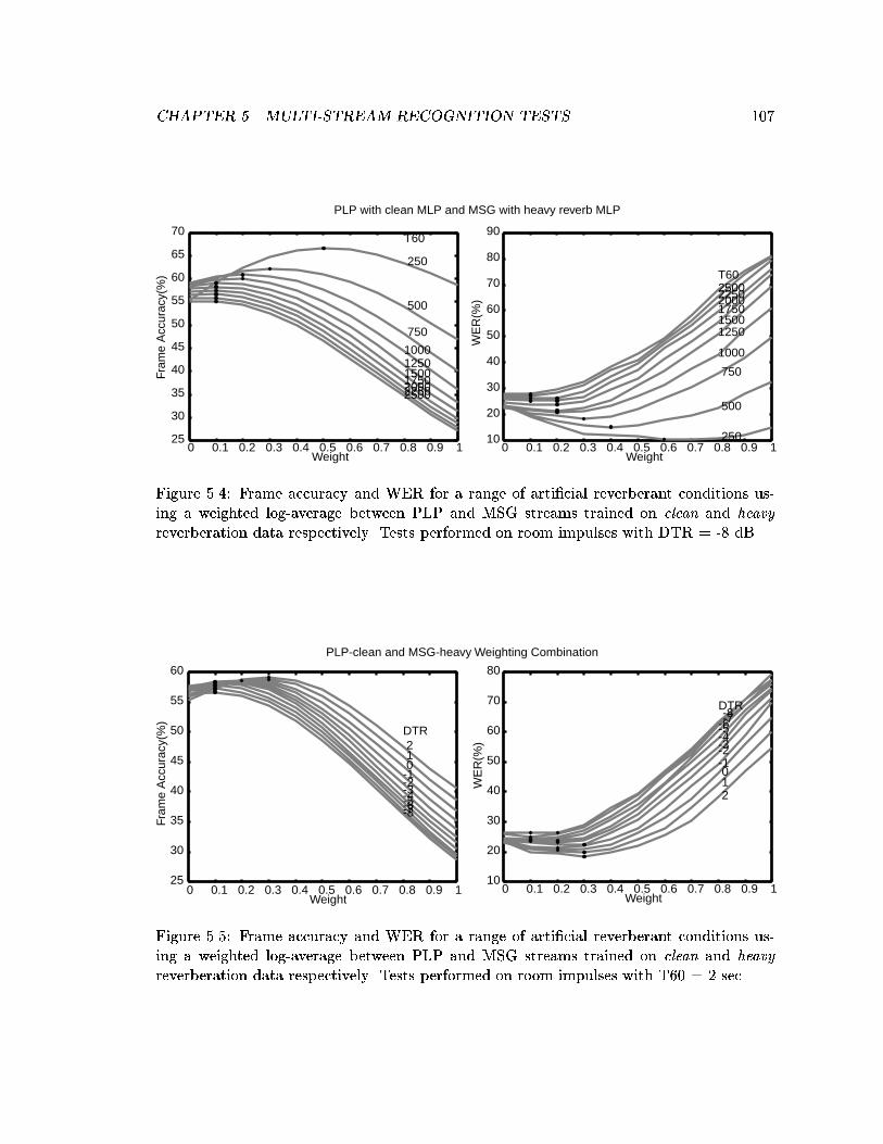
CHAPTER 5. MULTI-STREAM RECOGNITION TESTS 107
0 0.1 0.2 0.3 0.4 0.5 0.6 0.7 0.8 0.9 125
30
35
40
45
50
55
60
65
70
250
500
750
1000125015001750200022502500
T60
Weight
Fram
e A
ccur
acy(
%)
PLP with clean MLP and MSG with heavy reverb MLP
0 0.1 0.2 0.3 0.4 0.5 0.6 0.7 0.8 0.9 110
20
30
40
50
60
70
80
90
250
500
750
1000
125015001750200022502500T60
Weight
WE
R(%
)
Figure 5.4: Frame accuracy and WER for a range of arti�cial reverberant conditions us-ing a weighted log-average between PLP and MSG streams trained on clean and heavy
reverberation data respectively. Tests performed on room impulses with DTR = -8 dB.
0 0.1 0.2 0.3 0.4 0.5 0.6 0.7 0.8 0.9 125
30
35
40
45
50
55
60
-8-7-6-5-4-3-2-1 0 1 2DTR
Weight
Fram
e A
ccur
acy(
%)
PLP-clean and MSG-heavy Weighting Combination
0 0.1 0.2 0.3 0.4 0.5 0.6 0.7 0.8 0.9 110
20
30
40
50
60
70
80
-8-7-6-5-4-3-2-1 0 1 2
DTR
Weight
WE
R(%
)
Figure 5.5: Frame accuracy and WER for a range of arti�cial reverberant conditions us-ing a weighted log-average between PLP and MSG streams trained on clean and heavy
reverberation data respectively. Tests performed on room impulses with T60 = 2 sec.
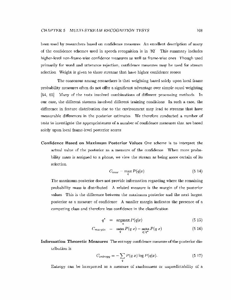
CHAPTER 5. MULTI-STREAM RECOGNITION TESTS 108
been used by researchers based on con�dence measures. An excellent description of many
of the con�dence schemes used in speech recognition is in [92]. This summary includes
higher-level non-frame-wise con�dence measures as well as frame-wise ones. Though used
primarily for word and utterance rejection, con�dence measures may be used for stream
selection. Weight is given to those streams that have higher con�dence scores.
The consensus among researchers is that weighting based solely upon local frame
probability measures often do not o�er a signi�cant advantage over simple equal weighting
[54, 65]. Many of the tests involved combinations of di�erent processing methods. In
our case, the di�erent streams involved di�erent training conditions. In such a case, the
di�erence in feature distribution due to the environment may lead to streams that have
measurable di�erences in the posterior estimates. We therefore conducted a number of
tests to investigate the appropriateness of a number of con�dence measures that are based
solely upon local frame-level posterior scores.
Con�dence Based on Maximum Posterior Values One scheme is to interpret the
actual value of the posterior as a measure of the con�dence. When more proba-
bility mass is assigned to a phone, we view the stream as being more certain of its
selection.
Cmax = maxq
P (qjx) (5.14)
The maximum posterior does not provide information regarding where the remaining
probability mass is distributed. A related measure is the margin of the posterior
values. This is the di�erence between the maximum posterior and the next largest
posterior as a measure of con�dence. A smaller margin indicates the presence of a
competing class and therefore less con�dence in the classi�cation.
q� = argmaxq
P (qjx) (5.15)
Cmargin = maxq
P (qjx)�maxq=q�
P (qjx) (5.16)
Information Theoretic Measures The entropy con�dence measure of the posterior dis-
tribution is
Centropy = �Xq
P (qjx) log P (qjx): (5.17)
Entropy can be interpreted as a measure of randomness or unpredictability of a
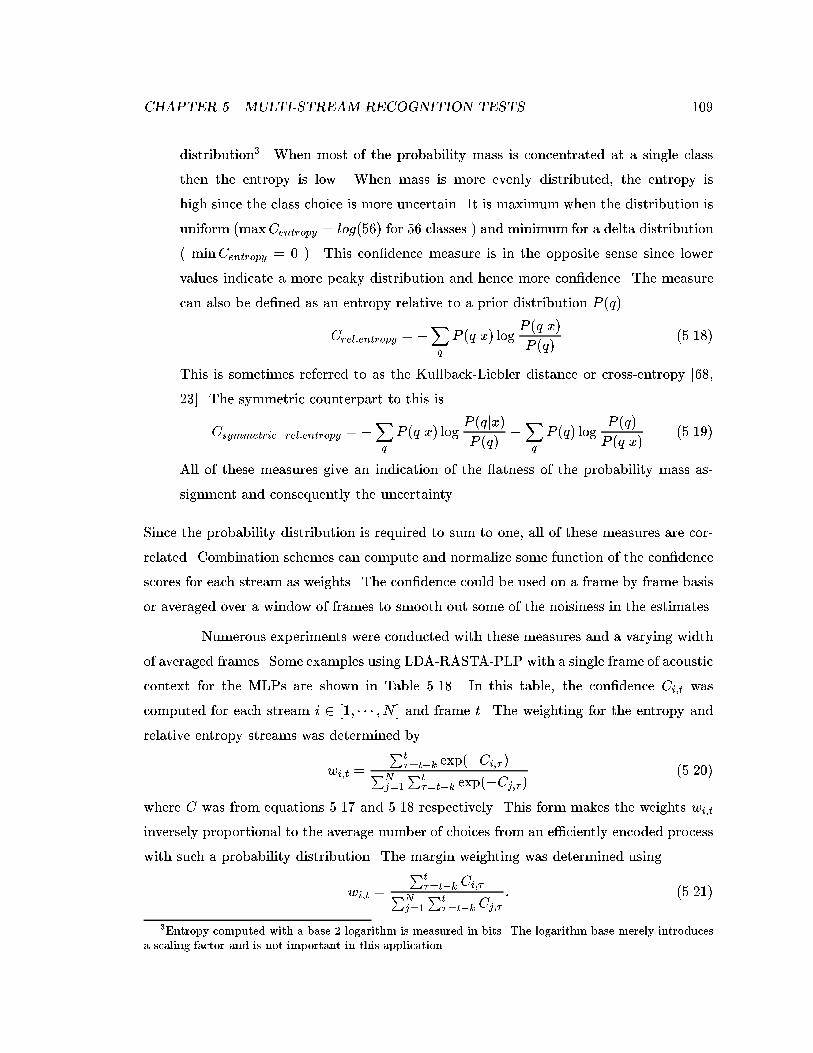
CHAPTER 5. MULTI-STREAM RECOGNITION TESTS 109
distribution3. When most of the probability mass is concentrated at a single class
then the entropy is low. When mass is more evenly distributed, the entropy is
high since the class choice is more uncertain. It is maximum when the distribution is
uniform (maxCentropy = log(56) for 56 classes ) and minimum for a delta distribution
( minCentropy = 0 ). This con�dence measure is in the opposite sense since lower
values indicate a more peaky distribution and hence more con�dence. The measure
can also be de�ned as an entropy relative to a prior distribution P (q).
Crel:entropy = �Xq
P (qjx) log P (qjx)P (q)
(5.18)
This is sometimes referred to as the Kullback-Liebler distance or cross-entropy [68,
23]. The symmetric counterpart to this is
Csymmetric�rel:entropy = �Xq
P (qjx) log P (qjx)P (q)
�Xq
P (q) logP (q)
P (qjx) (5.19)
All of these measures give an indication of the atness of the probability mass as-
signment and consequently the uncertainty.
Since the probability distribution is required to sum to one, all of these measures are cor-
related. Combination schemes can compute and normalize some function of the con�dence
scores for each stream as weights. The con�dence could be used on a frame by frame basis
or averaged over a window of frames to smooth out some of the noisiness in the estimates.
Numerous experiments were conducted with these measures and a varying width
of averaged frames. Some examples using LDA-RASTA-PLP with a single frame of acoustic
context for the MLPs are shown in Table 5.18. In this table, the con�dence Ci;t was
computed for each stream i 2 [1; � � � ; N ] and frame t. The weighting for the entropy and
relative entropy streams was determined by
wi;t =
Pt�=t�k exp(�Ci;� )PN
j=1
Pt�=t�k exp(�Cj;� )
(5.20)
where C was from equations 5.17 and 5.18 respectively. This form makes the weights wi;t
inversely proportional to the average number of choices from an e�ciently encoded process
with such a probability distribution. The margin weighting was determined using
wi;t =
Pt�=t�k Ci;�PN
j=1
Pt�=t�k Cj;�
: (5.21)
3Entropy computed with a base 2 logarithm is measured in bits. The logarithm base merely introducesa scaling factor and is not important in this application.
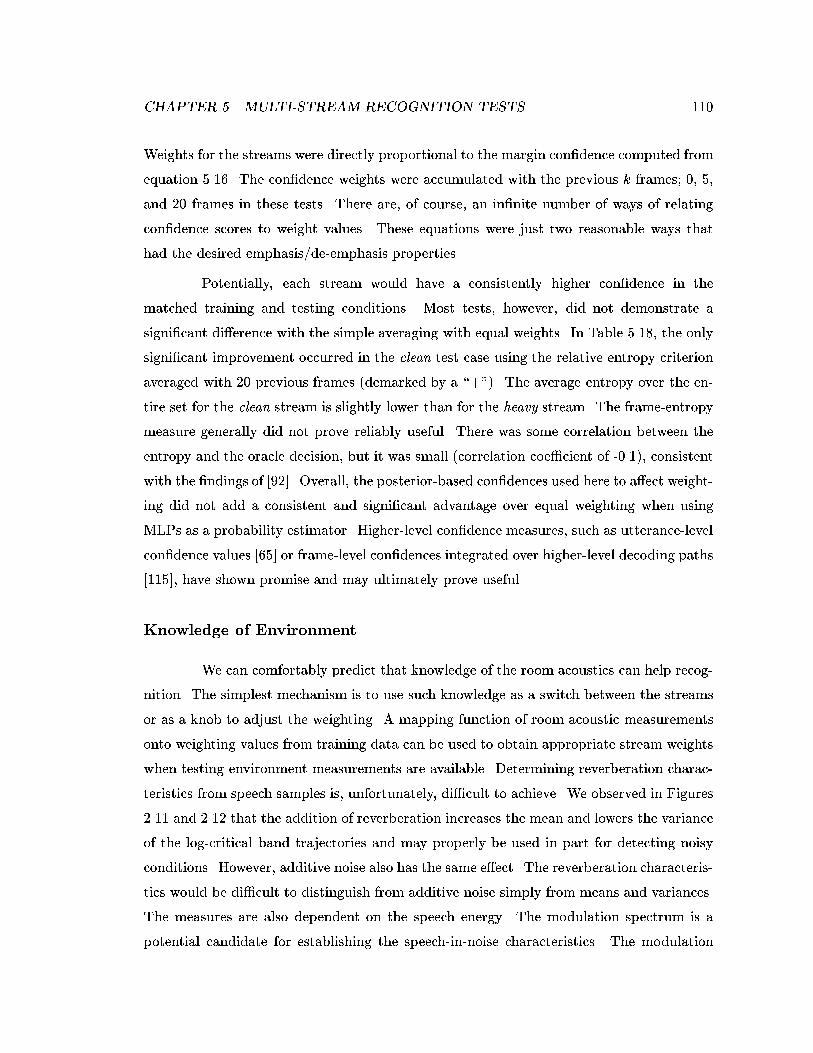
CHAPTER 5. MULTI-STREAM RECOGNITION TESTS 110
Weights for the streams were directly proportional to the margin con�dence computed from
equation 5.16. The con�dence weights were accumulated with the previous k frames; 0, 5,
and 20 frames in these tests. There are, of course, an in�nite number of ways of relating
con�dence scores to weight values. These equations were just two reasonable ways that
had the desired emphasis/de-emphasis properties.
Potentially, each stream would have a consistently higher con�dence in the
matched training and testing conditions. Most tests, however, did not demonstrate a
signi�cant di�erence with the simple averaging with equal weights. In Table 5.18, the only
signi�cant improvement occurred in the clean test case using the relative entropy criterion
averaged with 20 previous frames (demarked by a \+"). The average entropy over the en-
tire set for the clean stream is slightly lower than for the heavy stream. The frame-entropy
measure generally did not prove reliably useful. There was some correlation between the
entropy and the oracle decision, but it was small (correlation coe�cient of -0.1), consistent
with the �ndings of [92]. Overall, the posterior-based con�dences used here to a�ect weight-
ing did not add a consistent and signi�cant advantage over equal weighting when using
MLPs as a probability estimator. Higher-level con�dence measures, such as utterance-level
con�dence values [65] or frame-level con�dences integrated over higher-level decoding paths
[115], have shown promise and may ultimately prove useful.
Knowledge of Environment
We can comfortably predict that knowledge of the room acoustics can help recog-
nition. The simplest mechanism is to use such knowledge as a switch between the streams
or as a knob to adjust the weighting. A mapping function of room acoustic measurements
onto weighting values from training data can be used to obtain appropriate stream weights
when testing environment measurements are available. Determining reverberation charac-
teristics from speech samples is, unfortunately, di�cult to achieve. We observed in Figures
2.11 and 2.12 that the addition of reverberation increases the mean and lowers the variance
of the log-critical band trajectories and may properly be used in part for detecting noisy
conditions. However, additive noise also has the same e�ect. The reverberation characteris-
tics would be di�cult to distinguish from additive noise simply from means and variances.
The measures are also dependent on the speech energy. The modulation spectrum is a
potential candidate for establishing the speech-in-noise characteristics. The modulation
CHAPTER 5. MULTI-STREAM RECOGNITION TESTS 111
WER (%)Combination clean test light test heavy test
LDA-RASTA-PLP (clean Filters and MLP) alone 9.1 33.1 72.5LDA-RASTA-PLP (heavy Filters and MLP) alone 43.2 37.8 38.9
log-average equal 13.5 26.4 54.0
entropy 14.4 26.7 53.3entropy +5 frame 14.5 27.0 54.4entropy +20 frame 13.8 27.1 55.0rel. entropy 12.5 27.2 53.6rel. entropy +5 frame 12.4 27.3 54.2rel. entropy +20 frame 11.9 + 27.5 54.7margin 14.8 - 27.0 54.1margin +5 frame 14.4 26.9 54.8margin +20 frame 13.3 27.0 54.7
Table 5.18: WER Results from a frame-level weighted log-average combination of LDA-RASTA-PLP with clean and heavy trained MLP and LDA �lters using con�dence basedweighting. MLPs were trained with a single input frame of features. The \+" and \-"annotations mark two cases where the weighting produced WER that was respectivelysigni�cantly better and worse than the equal weighting.
spectrum of a test utterance can be computed with weight given to the stream with a
\closer" modulation spectral characteristic of its training set. This method would also
require further investigation. Pilot experiments reveal that the variance in the modulation
spectral estimates is relatively high, especially for the short utterances in the Numbers
corpus. Further, the room acoustics must typically be rather severe before it noticeably
impedes the modulation of the speech itself. Acoustic condition detection is a topic worthy
of further study.
5.6 Final Tests with Unseen Conditions and Best Stream
Combination
We present some �nal recognition experiments using 11 additional room impulses
previously unused in our experiments together with the light reverberation treated as the
unseen case in the multi-stream tests. As before, these room impulses were collected in
a varechoic chamber with re ective panels that were either opened or closed [113]. Three
sets of measurements with four microphones were used. The �rst set had 100% of the
CHAPTER 5. MULTI-STREAM RECOGNITION TESTS 112
Room impulse test WER %
Panels Mic. DTR T60 PLP stream MSG stream logavgopen(%) (dB) (s) clean heavy clean heavy merge
100 1 1 0.3 12.0 42.3 9.6 24.4 8.6 +100 2 1 0.3 10.6 43.0 9.2 23.5 7.7 +100 3 -1 0.3 12.1 39.9 10.8 24.1 8.9 +100 4 -1 0.3 11.7 41.6 10.1 24.7 9.8
43 1 1 0.5 22.2 30.8 13.9 23.7 11.0 +43 2 -3 0.5 21.4 33.3 15.3 23.3 11.7 +43 3 -2 0.5 22.3 31.1 17.6 23.6 11.9 +43 4 -5 0.5 24.2 31.4 18.9 23.5 13.5 +
0 1 -5 1 55.7 33.2 42.5 26.1 24.0 +0 2 -7 1 55.8 31.5 45.6 25.0 24.60 3 -7 1 60.6 33.8 52.3 26.7 29.6 -0 4 -9 1 59.9 35.9 53.0 26.8 29.5 -
Table 5.19: Final tests using four PLP and MSG streams trained in clean and heavy re-verberation. Combination using log-average posteriors with equal weighting. The +(-)annotations mark where the log-average posterior merging produced WER that was sig-ni�cantly better (worse) than the single streams.
panels open, giving rise to less re ections and a less reverberant room. In the second set,
43% of the panels were open. The light reverberation tests used previously were of the
�rst microphone in this set. The �nal set had all of the panels closed, resulting in a more
reverberant environment.
Combinations using PLP and MSG yielded the best word recognition results
overall. We used them here in a four stream setting where MLPs were trained using PLP
and MSG data separately in both the clean and heavy reverberation environments. The
combination method of log-averaging consistently produced slightly better results in tests
with the unseen environment and are used here. Word error results are listed in Table 5.19.
The �rst 8 rows (corresponding to 100% and 43% open panels) had lower re-
verberation times. Equal weighting was therefore satisfactory and improved results for
most of the cases, by as much as 30% relative to the best stream. MSG was constructed
for robustness in reverberation and performed consistently better than PLP. The MSG
stream trained on clean performed the best on the less reverberated conditions. The last 4
rows (no open panels) included more severe reverberation. In these cases the MSG stream
trained on heavy reverberation performed the best. The combination for these scores had
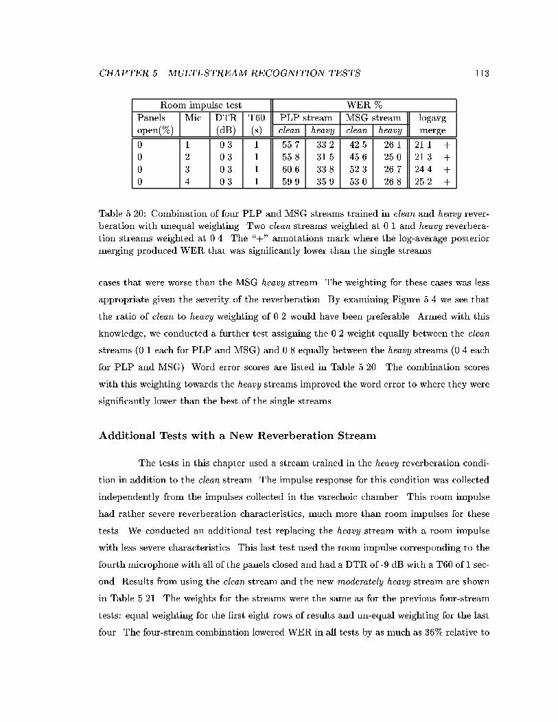
CHAPTER 5. MULTI-STREAM RECOGNITION TESTS 113
Room impulse test WER %
Panels Mic. DTR T60 PLP stream MSG stream logavgopen(%) (dB) (s) clean heavy clean heavy merge
0 1 0.3 1 55.7 33.2 42.5 26.1 21.1 +0 2 0.3 1 55.8 31.5 45.6 25.0 21.3 +0 3 0.3 1 60.6 33.8 52.3 26.7 24.4 +0 4 0.3 1 59.9 35.9 53.0 26.8 25.2 +
Table 5.20: Combination of four PLP and MSG streams trained in clean and heavy rever-beration with unequal weighting. Two clean streams weighted at 0.1 and heavy reverbera-tion streams weighted at 0.4. The \+" annotations mark where the log-average posteriormerging produced WER that was signi�cantly lower than the single streams.
cases that were worse than the MSG heavy stream. The weighting for these cases was less
appropriate given the severity of the reverberation. By examining Figure 5.4 we see that
the ratio of clean to heavy weighting of 0.2 would have been preferable. Armed with this
knowledge, we conducted a further test assigning the 0.2 weight equally between the clean
streams (0.1 each for PLP and MSG) and 0.8 equally between the heavy streams (0.4 each
for PLP and MSG). Word error scores are listed in Table 5.20. The combination scores
with this weighting towards the heavy streams improved the word error to where they were
signi�cantly lower than the best of the single streams.
Additional Tests with a New Reverberation Stream
The tests in this chapter used a stream trained in the heavy reverberation condi-
tion in addition to the clean stream. The impulse response for this condition was collected
independently from the impulses collected in the varechoic chamber. This room impulse
had rather severe reverberation characteristics, much more than room impulses for these
tests. We conducted an additional test replacing the heavy stream with a room impulse
with less severe characteristics. This last test used the room impulse corresponding to the
fourth microphone with all of the panels closed and had a DTR of -9 dB with a T60 of 1 sec-
ond. Results from using the clean stream and the new moderately heavy stream are shown
in Table 5.21. The weights for the streams were the same as for the previous four-stream
tests: equal weighting for the �rst eight rows of results and un-equal weighting for the last
four. The four-stream combination lowered WER in all tests by as much as 36% relative to
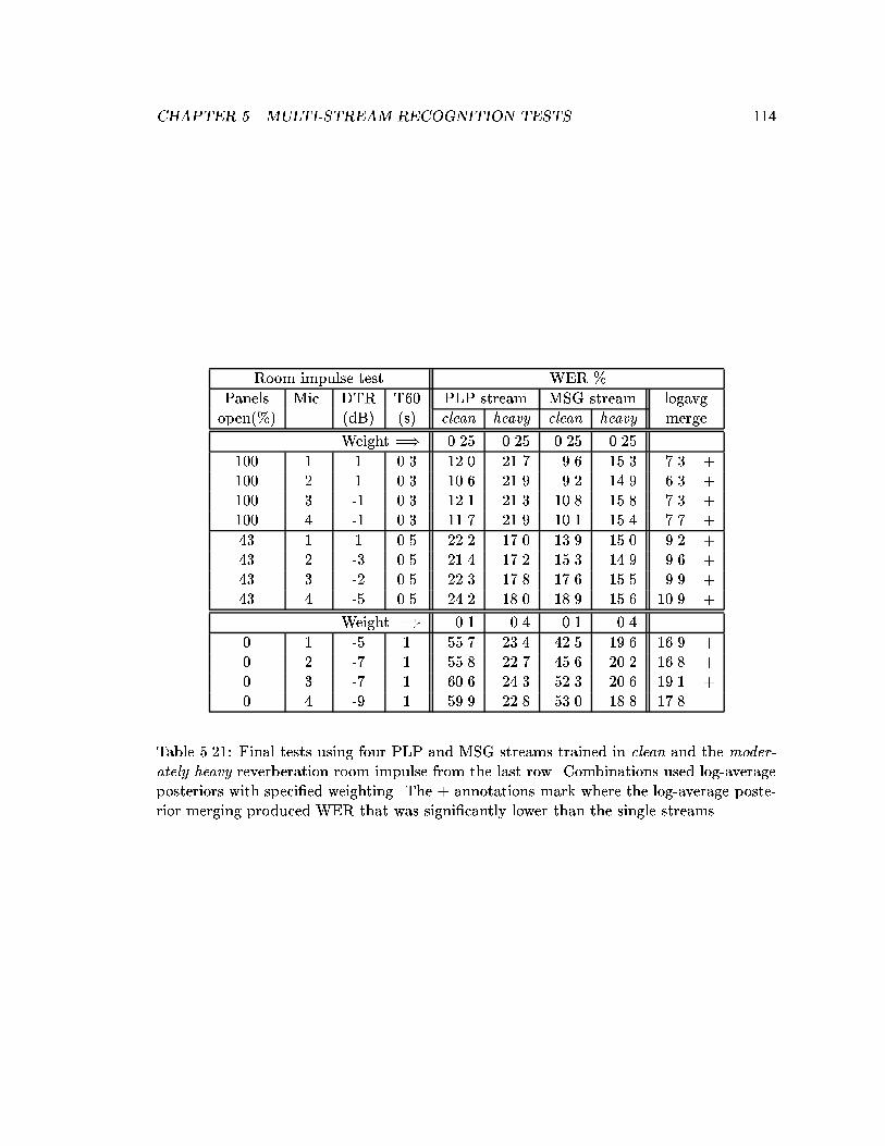
CHAPTER 5. MULTI-STREAM RECOGNITION TESTS 114
Room impulse test WER %
Panels Mic. DTR T60 PLP stream MSG stream logavgopen(%) (dB) (s) clean heavy clean heavy merge
Weight =) 0.25 0.25 0.25 0.25
100 1 1 0.3 12.0 21.7 9.6 15.3 7.3 +100 2 1 0.3 10.6 21.9 9.2 14.9 6.3 +100 3 -1 0.3 12.1 21.3 10.8 15.8 7.3 +100 4 -1 0.3 11.7 21.9 10.1 15.4 7.7 +
43 1 1 0.5 22.2 17.0 13.9 15.0 9.2 +43 2 -3 0.5 21.4 17.2 15.3 14.9 9.6 +43 3 -2 0.5 22.3 17.8 17.6 15.5 9.9 +43 4 -5 0.5 24.2 18.0 18.9 15.6 10.9 +
Weight =) 0.1 0.4 0.1 0.4
0 1 -5 1 55.7 23.4 42.5 19.6 16.9 +0 2 -7 1 55.8 22.7 45.6 20.2 16.8 +0 3 -7 1 60.6 24.3 52.3 20.6 19.1 +0 4 -9 1 59.9 22.8 53.0 18.8 17.8
Table 5.21: Final tests using four PLP and MSG streams trained in clean and the moder-ately heavy reverberation room impulse from the last row. Combinations used log-averageposteriors with speci�ed weighting. The + annotations mark where the log-average poste-rior merging produced WER that was signi�cantly lower than the single streams.
CHAPTER 5. MULTI-STREAM RECOGNITION TESTS 115
the best of the single streams. Only the last row of results, corresponding to the condition
for one of the streams, did not lower the WER signi�cantly. Using this less severe room
impulse as one of the streams yielded results that were better than when using the more
severe heavy stream by between 15% and 40% relative. The new reverberation impulse had
characteristics closer to the testing data environments with better performance among the
single stream tests. This allowed for word error rates in the unseen environments that are
much more usable.
5.7 Discussion
By and large the environment in which the MLP probability estimator is trained is
the overriding factor on the performance in di�erent reverberant environments. Even with
robust feature extraction routines the di�erence in the feature distributions associated with
room characteristics varies widely enough to cause severe degradation in word recognition.
From the single stream tests in reverberant environments it seems likely that even given an
arbitrarily large number of trained parameters, the performance of a system trained with
clean data would not approach the performance of a system trained with heavy reverber-
ation on tests with heavy reverberation. In fact it would be in danger of over-�tting the
training data. Extrapolating, this clean-trained single stream system will only be e�ective
in approximately clean environments. The e�ects of a more highly reverberant environ-
ments on the feature distributions are too great. Single streams trained on some type
of reverberation can sometimes produce better results with other types of reverberation
compared to the performance of the clean-trained stream. The feature distribution of the
new reverberant environment may deviate further from the clean training data than from
the reverberation training data and therefore can result in better probability estimates. It
would then seem prudent to include in the system some measure of what the distribution
might look like in such an environment.
By employing a switching algorithm a system having trained elements from two
environments should broaden the range of graceful degradation due to the environment.
An encouraging side-e�ect from the combination experiments, however, is that a combined
system can perform better in a new environment than a single environment system can;
this is an example where the whole can be worth more than the sum of the parts. The
CHAPTER 5. MULTI-STREAM RECOGNITION TESTS 116
probability estimates from each stream re-enforce each other when frame decisions agree
while moderating the set of choices when they disagree.
The most encouraging results occurred when a two-stream system had streams
that were trained in di�erent environments and then presented with data from an unseen
environment. Scores in the unseen environment were superior in the combined system
than the singly trained systems. The unfortunate side e�ect was a penalty in either of the
matched conditions. In this situation, one stream was at its best and the other stream
was at its worst. In such cases, the worse stream harmed the combination more than
help, though the resulting combination still performed closer to the better stream. A non-
linear merging scheme or a dynamic weighting scheme may improve the results. An extra
input or measure that can intelligently switch o� the worse stream appropriately would
rectify problems in the matched cases. When such information is not available though,
the compromised performance in matched cases can still be a reasonable trade-o�. Real
deployed ASR systems will typically be presented with speech in an alternative environment
to its training environment.
The tests here were constructed such that the two training conditions were at the
more extreme ends of the reverberation spectrum: clean and heavy. This would make the
unseen condition more likely to have reverberation characteristics lie in between these two
extremes. This setup was chosen to broaden the range of graceful performance degradation
the most. In the earlier single-stream tests, both the clean and light single stream systems
performed abysmally on heavy reverberation. Using these two streams in combination
improved results to some extent in heavy reverberation but were still unacceptable for use.
Using the heavy trained stream instead yields results that are much more acceptable over
a wider range of room impulses, as the �nal tests in the last section indicated. Using a
less severe reverberation stream in lieu of the heavy room impulse improved results further.
The characteristics of the new stream were closer to the testing environments. It would
also be of interest to see the e�ects of adding a third stream trained with reverberation
characteristics between the extreme ones used. Due to the compromised performance in
matched cases arbitrarily high numbers of streams may yield diminishing performance
gains.
A trend in the experiments was that the PLP and MSG streams combined more
e�ectively than RASTA-PLP with di�erent temporal �lter sets. Intuitively, PLP and
CHAPTER 5. MULTI-STREAM RECOGNITION TESTS 117
MSG process speech much more di�erently and therefore should be more prone to making
di�erent kinds of errors. For example, in clean training and testing experiments, 71% of
the misclassi�ed frames using the clean LDA �lters in RASTA-PLP co-occurred with the
heavy LDA �lters. However, only 67% of the frame errors made by a clean PLP stream
co-occurred with frame errors from a clean MSG stream. Similarly, with clean and heavy
RASTA-PLP streams and a light reverberation test, 72% of the frame errors of the clean
stream were also made by the heavy stream while 66% of the errors of the clean PLP stream
overlapped with the heavyMSG stream. This di�erence in the number of overlapping frame
errors needs to be interpreted with a considerable degree of caution due to the complex
relationship between frame accuracy and word error.
The combination experiments, as with single-stream experiments, also provided
a number of examples where a system with a lower frame accuracy performed signi�cantly
better for word recognition. For example, we conducted four stream experiments using
RASTA-PLP (not listed) with both clean and heavy LDA �lters with MLPs trained on
clean and heavy reverberation data. All of the frame accuracies were between 10% and
20% better relative to the four-stream PLP-MSG frame accuracy scores corresponding to
the tests in Table 5.17. However the word errors for four-stream LDA-RASTA-PLP were up
to 88% worse relative. Another example was that the frame accuracies for the four-stream
PLP-MSG combinations were 20% worse relative to the two-stream PLP-MSG systems
while the word error either remained constant or improved. A possible explanation for
this result is that not all of the frames are equally important for word recognition. The
combined system may be reinforcing the posterior scores for the frames that are crucial to
word recognition. Reinforcing occurs at those frames where most or all of the streams agree
while making more uncertain the remaining frames. This may be hindering the Viterbi
search from following false paths caused by frames with high probability in the incorrect
class. Again, further research and a more complete diagnostic would be required to arrive
at a convincing explanation.
The language model scaling parameter in the Chronos decoder was re-tuned
using the CV set for each recognition run to yield the lowest word error on that set. In
many tests the best language model scaling factors were similar. In other tests (for example,
between MSG and RASTA-PLP) this parameter was di�erent. Di�erent language-model
scaling parameters were also used between the two-stream and four-stream systems; the
CHAPTER 5. MULTI-STREAM RECOGNITION TESTS 118
best language model scaling parameter was lower for the four-stream than for the two-
stream system, meaning that the acoustic probabilities had more relative in uence in the
overall decoding. This can also be telling in that it o�ers some indication that the acoustic
probability stream was more reliable and needed less aid by language constraints. The
decoding parameter was constantly re-tuned between the tests to give an indication of the
best word error achievable with the decoder and in order to remove the e�ect of a possibly
sub-optimal selection of parameters. Di�erent front-end components may sometimes be
poorly matched to speci�c decoding constraints, models and parameters. Forced alignment
is sometimes used to produce training data that better matches the pronunciation models
to the acoustic probability training. However, pilot tests using this method did not bene�t
our experiments. Despite the many real and potential shortcomings, the combination
of streams trained in di�erent environments consistently improved recognition in unseen
environments.
119
Chapter 6
Conclusion
A common problem with current ASR systems is that the performance can de-
grade signi�cantly when presented with speech emanating from a di�erent acoustic envi-
ronment than was seen during training. An important cause of this is that the feature
distribution to which the ASR system is trained no longer matches that of a new environ-
ment. A partial remedy is to additionally train system components on feature distributions
from di�erent environments in a multi-stream system. A bene�t of the multi-stream ap-
proach is that it can capitalize on the strengths of more than one approach for maintaining
robustness to acoustic degradation. Advances in any of the components of the system can
be readily integrated into the multi-stream system.
Multi-stream approaches can take a number of forms. The approach used in this
thesis employed multiple front-end acoustic modeling stages whose acoustic probability
estimates were then merged for further processing by the word-recognition decoder. Each
of the front-end stages was trained to improve phone classi�cation in a speci�c acoustic
environment. With multiple front-end stages trained in di�erent conditions, the range of
environments where the ASR system can maintain reasonable performance increases. Room
reverberation was the principal type of acoustic distortion investigated in the experiments,
though preliminary tests also included some examples of additive background noise.
The evolution of this work proceeded in two stages. The �rst stage involved train-
ing front-end stages to perform optimally in sample acoustic environments. A phone class
discriminant criterion was used in training the front-end acoustic modeling. The second
CHAPTER 6. CONCLUSION 120
stage tested these trained front-end modeling components in combination. Of particular
interest was the performance in acoustic environments other than the ones used in training.
6.1 Discriminant Feature Extraction
We investigated a means of improving the performance of the front-end system
over a range of acoustic environments. In addition to training the probability estimator
we modi�ed the speech signal processing to improve class discrimination in the degraded
acoustic environment. Rather than develop a novel processing technique for each envi-
ronment we modi�ed the temporal �ltering of existing preprocessing algorithms. The
general approach was to apply discriminative learning to the time-frequency plane. Since
the MLP probability estimator already incorporated non-linear discriminant training along
the frequency-related direction, we added a discriminant component along the temporal
dimension. The temporal �lters were derived using Linear Discriminant Analysis. The
LDA �lters were derived on a task-independent data set to promote generality.
Linear Discriminant Analysis has proven to be a powerful technique in statistical
data analysis. As applied in this thesis, LDA automatically generates an ordered set
of discriminant linear �lters that operate on the temporal trajectories of the frequency
energies. The temporal �lters derived with LDA bear striking similarity to the standard
RASTA �lter that passes the modulation frequencies between 1 and 12 Hz. Since the
acoustic environment modi�es the critical-band energy trajectories and since the LDA
�lters are computed from these modi�ed trajectory distributions, we expected to see some
modi�cations to the resulting temporal �lters with respect to the acoustic environment.
In the presence of reverberation there is a tendency for the band-pass range to narrow
towards the more syllabic rate of 5 Hz. This is consistent with evidence that syllabic rates
harbor some perceptual stability. In cases with added background noise, there is also some
narrowing of the preferred frequency range, though not as severe.
Using the derived �lters almost uniformly improves frame-classi�cation accuracy.
This is expected since LDA �lters were designed to distinguish among phone classes. Tests
with RASTA-PLP also indicate that this can lead to improvements in word recognition.
The improvements between the di�erent �lters can be mitigated or made redundant, how-
ever, by allowing the MLP probability estimator access to a wider acoustic context of
CHAPTER 6. CONCLUSION 121
frames. With a wider acoustic context, the MLP training implicitly includes temporal pro-
cessing. Further, MLPs are discriminatively trained in a nonlinear manner that is complex
and inherently more powerful than the linear �lters. Word recognition improvements were
also not forthcoming in tests using PLP cepstra and MSG even while the frame accuracy
was maintained or improved upon.
In our experiments, a single bank of �lters was derived to distinguish among all
phones. The �lters in the individual frequency bands were generally consistent though
sometimes have di�erent preferred modulation frequency ranges. This was due in part to
the relative severity to which an acoustic environment a�ected di�erent frequency ranges
and in part to the di�erences in the temporal and frequency characteristics among subsets of
phonetic classes. Future work may involve further discrimination within sets of phones for a
�ner discrimination, similar to the TRAPS �lters derived by Sharma [99, 98, 51]. It may be
useful to observe the e�ect of acoustic environments on these �lters. Further discriminative
training based upon criteria distinct from those used in LDA may also be investigated.
However, due to the inconsistent gains in word recognition using �lters optimized for phone
classi�cation, such an e�ort may result in disappointing gains. Kanedera and Arai found
through repeated ASR experiments that modulation spectral components below 16 Hz
yielded the highest word recognition accuracy. Components ranging from 2 and 8 Hz were
the most important for ASR [58, 59, 5]. The data-driven temporal �lters consistently
preserve these lower modulation frequency rates where the speech information resides.
Further parsing of this frequency range can give rise to improved classi�cation between
phones at the frame level but currently gives diminishing returns in word recognition
tests. What remains arguably important however is that the modulation rates where
the phonetically relevant components of the speech reside be preserved in some manner in
the feature processing.
6.2 Multi-Stream Combinations
With front-end stages that were trained to speci�c acoustic environments, the en-
suing work consisted of experiments with combining these stages in a multi-stream setting.
A number of tests were conducted using many of the techniques found in the literature.
Optimal methods of combining such probability streams remains a research issue. Con-
CHAPTER 6. CONCLUSION 122
sistent with many research results, we found that simple averaging combinations of the
log-probability streams provided reasonable and e�ective results, particularly when com-
bining PLP trained on clean speech and MSG trained on reverberant speech. This simple
method also allows for stream weighting that facilitates emphasizing (or de-emphasizing)
streams should additional information concerning the acoustic environment warrant it.
Tests using several room impulses with various stream weights indicate that com-
bined systems can improve upon the recognition accuracy of the system above a single
stream system. Performance degradation due to the acoustic environment can be miti-
gated by having a system trained in more than one environment. We chose to train our
combined system in the extreme cases of clean speech and heavy reverberation. Doing
so broadened the range of reasonable performance when confronted with data associated
with unknown reverberation characteristics. In these cases, the probability estimates from
the constituent streams served to reinforce each other enough to improve performance.
An apparent caveat is that a stream that performed very badly individually degraded the
performance of the higher quality streams. This can be seen in the matched condition
cases. In these instances, the introduction of a weighting knob or computed information
about the acoustic environment could help maintain recognition rates considerably. Tests
in which we adjusted these knobs and observed the results were signi�cantly better than
the evenly weighted feature streams.
The recognition tests were conducted using a hybrid ANN-HMM ASR system. It
would be worthwhile to repeat many of these experiments on a GMM-HMM system. Many
techniques, for example Maximum Likelihood Linear Regression [69], exist for adapting
models in these systems. It would be useful to con�rm that the improvements using multi-
ple front-end acoustic modeling stages trained in di�erent environments would also bene�t
systems that contain methods that attempt to account for such di�erences. Further, ex-
periments using local posterior measures to adjust the relative weighting yielded mediocre
gains in our tests. This was due to the noisiness in the local measures and possibly the
types of errors, often pathological, that the MLP produced. Some researchers have found
that frame-level posterior-based con�dence measures, although useful for word and utter-
ance rejection tasks, were less useful for stream weighting [65]. Higher-level con�dence
measures or frame-level measures integrated into higher-level measures, on the other hand,
should be useful here and should be investigated. Many of these types of measures are
CHAPTER 6. CONCLUSION 123
implementation or decoder speci�c, non-trivial to calculate, and were outside the scope
of this work. Con�dence measures, whether for utterance rejection or stream weighting,
remains the subject of on-going research.
6.3 Contribution and Future Work
This thesis has demonstrated that combinations of front-end acoustic modeling
components that have been trained in heterogeneous acoustic conditions can improve ASR
robustness to untrained acoustic conditions. Discriminatively trained temporal �lters, in
addition to the discriminatively trained MLP probability estimator, were used to improve
each streams performance in a sample acoustic condition. We found that this method con-
sistently improved phone classi�cation at the frame level. For the task of word recognition,
a single-stream system based on this method was only useful in certain cases. On tests
with unseen reverberation, the multi-stream system having components trained in both
clean and heavy reverberation produced results signi�cantly superior to the system trained
solely in one condition. Combination results appeared to be best when each of the streams
was based upon di�erent preprocessing strategies.
The multi-stream approach has been rapidly gaining attention within the ASR
community. Many have found that new experimental system components that sometimes
yielded unsatisfactory performance in isolation would boost performance when used in
combination with other approaches. Though the subject of feature-stream combination
has been studied by many researchers, optimal combination methods remain elusive; em-
pirical results often show that theoretically justi�able strategies do not necessarily perform
best. The best combination method can be dependent on the kinds of streams involved, the
type of system, and even the recognition task. Unfortunately, there is not yet a principled
way of determining the best combinations and best streams to combine other than to per-
form exhaustive testing. A hindrance to this is the combinatorial explosion of the number
of experiments. This factor also caused us to limit our experiments to simple combination
methods with a small number of streams. Given the number of possible combination meth-
ods and the number of possible feature streams, further multi-stream work would bene�t
from a means of predicting which feature streams and stream combination strategies would
be most successful. Ellis and Bilmes have recently tested conditional mutual information
CHAPTER 6. CONCLUSION 124
between streams as a candidate prediction tool in this area [30]. Their results suggest that
the mutual information between streams can indicate the classi�er merging potential from
two feature streams and provides a good starting point for further investigation into fea-
ture stream combination. For combination strategies, Bilmes and Kirchho� have recently
tested new combination methods based on speci�c independence assumptions with encour-
aging results [8]. They used directed acyclic graphical models as a tool for constructing
combination methods with explicit statistical properties.
A recurring di�culty in our experiments was the complex relationship between
the frame accuracy and the overall word recognition rate. There were repeated cases where
an improvement in frame accuracy did not give rise to similar improvements in word recog-
nition. This is a common observation when experimenting with complex systems where
a system component is optimized separately from the entire system. Our optimization of
the front-end acoustic modeling was based on phonetic classi�cation at the frame level.
This optimization neglected the complex interaction with the rest of the system, includ-
ing the pronunciation and language models, as well as the decoding algorithm. Although
high frame accuracy is arguably important for good word recognition, there is an apparent
mismatch between the criterion we used for good phone classi�cation and the criterion for
optimal word recognition. With this contradiction facing us, it is di�cult to determine
proper front-end and front-end combinations without doing exhaustive testing including
word recognition. Future work should analyze the interaction of the frame level posteriors
and the maximum a posteriori decoding. Our preliminary study in Appendix E indicate
that not all of the frame errors carry the same importance for the word recognition and
that the locations of these errors are signi�cant. A starting point of further work could
be to conduct further diagnostic tests of the ASR system in a style similar to that which
Greenberg and associates did on Switchboard ASR results [42, 41]. Tests using data with
varying degrees and types of frame errors together with various indicators of location (e.g.
onsets, nuclei, and coda of phones or syllables) as well as phone confusion and segmenta-
tion can be computed and compared with recognition output. Results from such analysis
may become instrumental in the future design of front-end acoustic modeling methods and
combinations.
125
Appendix A
Recognition Units
Recognition tests in this work used a subset of the Oregon Graduate Institute
(OGI) Numbers corpus [19]. The subset used consisted of utterances that had phonetic
transcriptions. Utterances that had non-number words such as \dash" were eliminated
from this subset, though some �lled-pauses were kept. A vocabulary of this corpus subset
is listed in Table A.1.
The ICSI ASR system uses 56 context independent monophone units. These are
listed in Table A.2 together with example words for pronunciation1. Due to the small
vocabulary of the Numbers corpus, only 32 of the 56 phonemes appear in the Numbers
corpus. For �lter derivation, the OGI Stories corpus was used. This corpus was better
suited to deriving temporal �lters due to the length of the utterances and the more com-
plete phonetic coverage. The independence of this corpus from the Numbers corpus also
promoted testing the generality of the derived LDA �lters.
1This table was adapted from one courtesy of Su-Lin Wu, Eric Fosler-Lussier, and Charles Wooters.
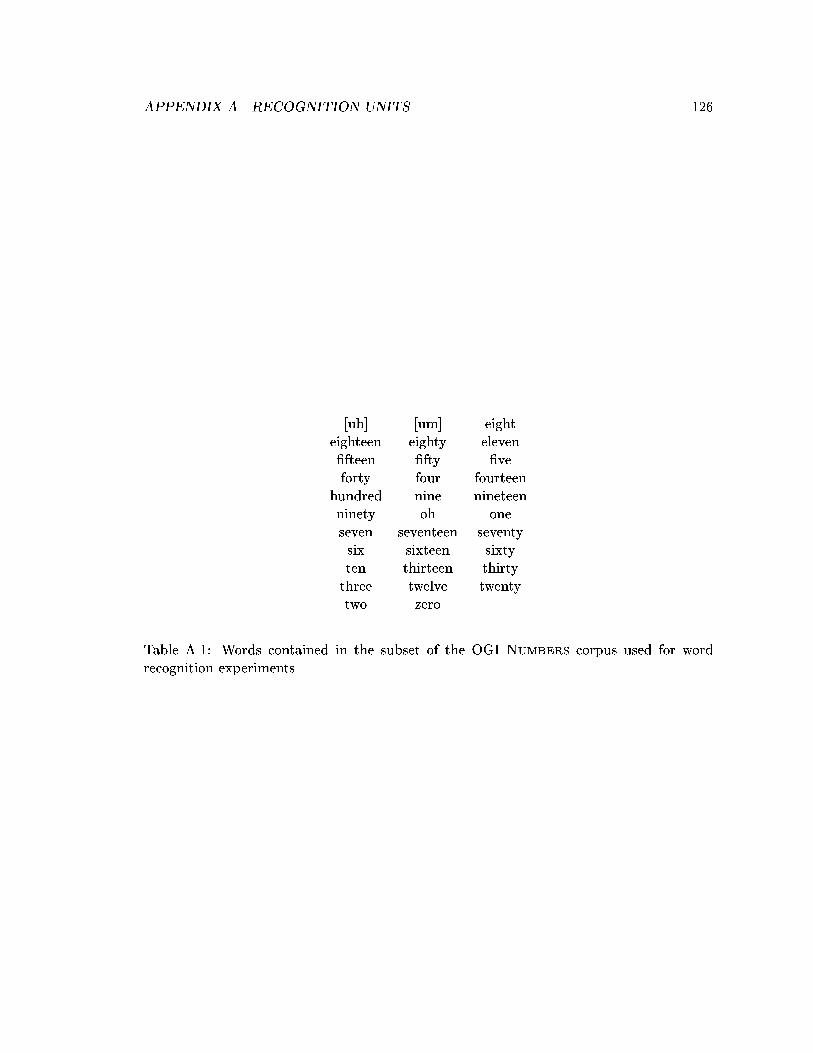
APPENDIX A. RECOGNITION UNITS 126
[uh] [um] eighteighteen eighty eleven�fteen �fty �veforty four fourteen
hundred nine nineteenninety oh oneseven seventeen seventysix sixteen sixtyten thirteen thirtythree twelve twentytwo zero
Table A.1: Words contained in the subset of the OGI Numbers corpus used for wordrecognition experiments.
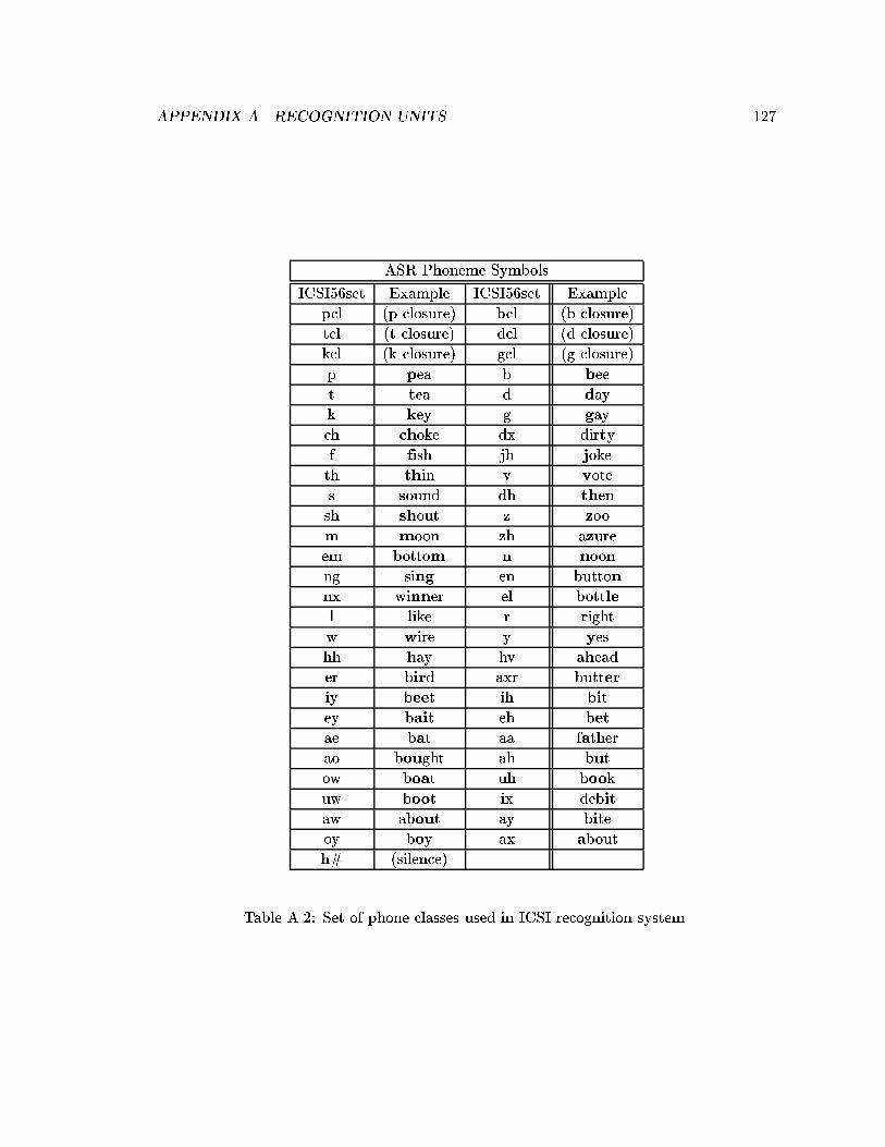
APPENDIX A. RECOGNITION UNITS 127
ASR Phoneme Symbols
ICSI56set Example ICSI56set Example
pcl (p closure) bcl (b closure)
tcl (t closure) dcl (d closure)
kcl (k closure) gcl (g closure)
p pea b bee
t tea d day
k key g gay
ch choke dx dirty
f fish jh joke
th thin v vote
s sound dh then
sh shout z zoo
m moon zh azure
em bottom n noon
ng sing en button
nx winner el bottle
l like r right
w wire y yes
hh hay hv ahead
er bird axr butter
iy beet ih bit
ey bait eh bet
ae bat aa father
ao bought ah but
ow boat uh book
uw boot ix debit
aw about ay bite
oy boy ax about
h# (silence)
Table A.2: Set of phone classes used in ICSI recognition system.
128
Appendix B
Temporal LDA Filters with
Phonetic Units
This appendix contains detailed plots of the LDA �lters derived from log critical
band trajectories. Figures B.1, B.2, and B.3 contain the three principal LDA �lters derived
with clean data, highly reverberated data and data with factory noise added at 10 dB SNR,
respectively. These plots illustrate the similarity in impulse and frequency response between
the �lters using a sampling of the frequency bands for clarity. The second, fourth, eighth,
and twelfth bands centered at 250, 450, 1000, and 1850 Hz respectively are presented. There
are slight di�erences between the frequency responses of the lower bands and the others;
the �lters from the lower bands tend to pass slightly lower modulation frequencies for the
non-clean cases. In the presence of heavy reverberation, for example, there is a pronounced
lowering in the preferred frequency ranges of the modulation spectra. Di�erences between
the lower and higher bands are also more evident with lower bands passing the lower
frequencies. This is consistent with reverberation being most evident at the lower portions
of the spectrum. Factory noise also demonstrates some lowering of the frequency ranges
though not as much.
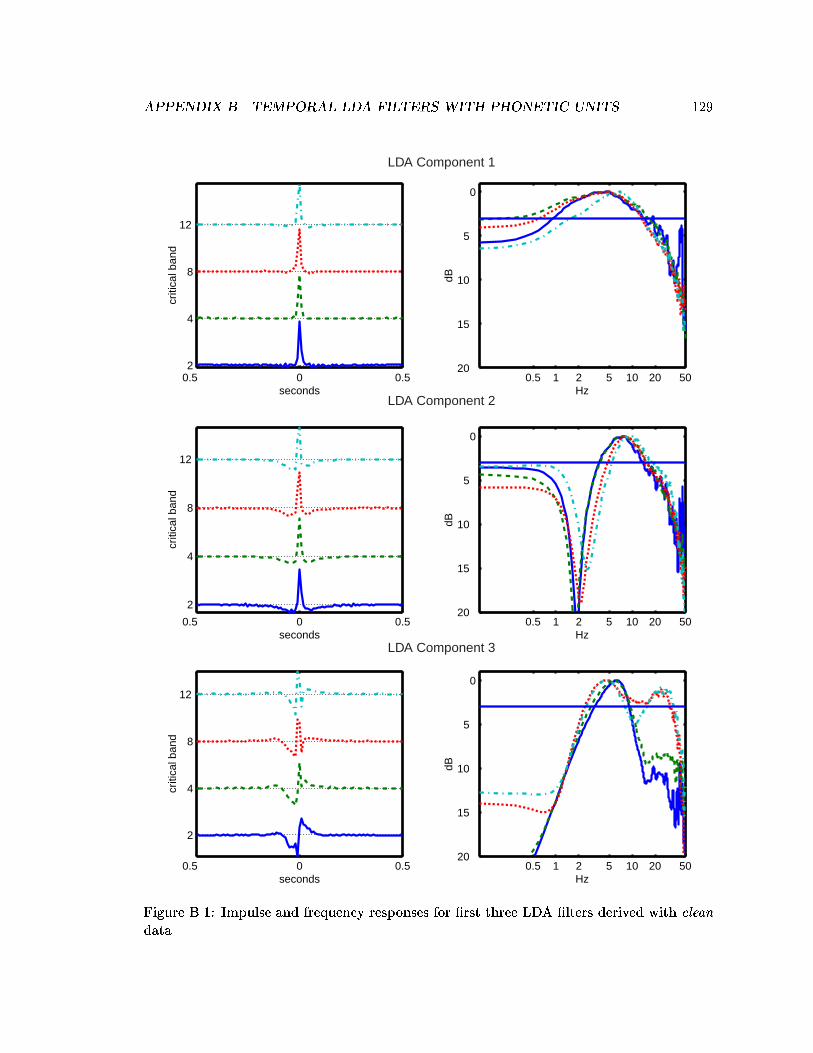
APPENDIX B. TEMPORAL LDA FILTERS WITH PHONETIC UNITS 129
0.5 0 0.5 2
4
8
12
seconds
criti
cal b
and
0.5 1 2 5 10 20 5020
15
10
5
0
Hz
dB
0.5 0 0.5
2
4
8
12
seconds
criti
cal b
and
0.5 1 2 5 10 20 5020
15
10
5
0
Hz
dB
0.5 0 0.5
2
4
8
12
seconds
criti
cal b
and
0.5 1 2 5 10 20 5020
15
10
5
0
Hz
dB
LDA Component 1
LDA Component 2
LDA Component 3
Figure B.1: Impulse and frequency responses for �rst three LDA �lters derived with clean
data.
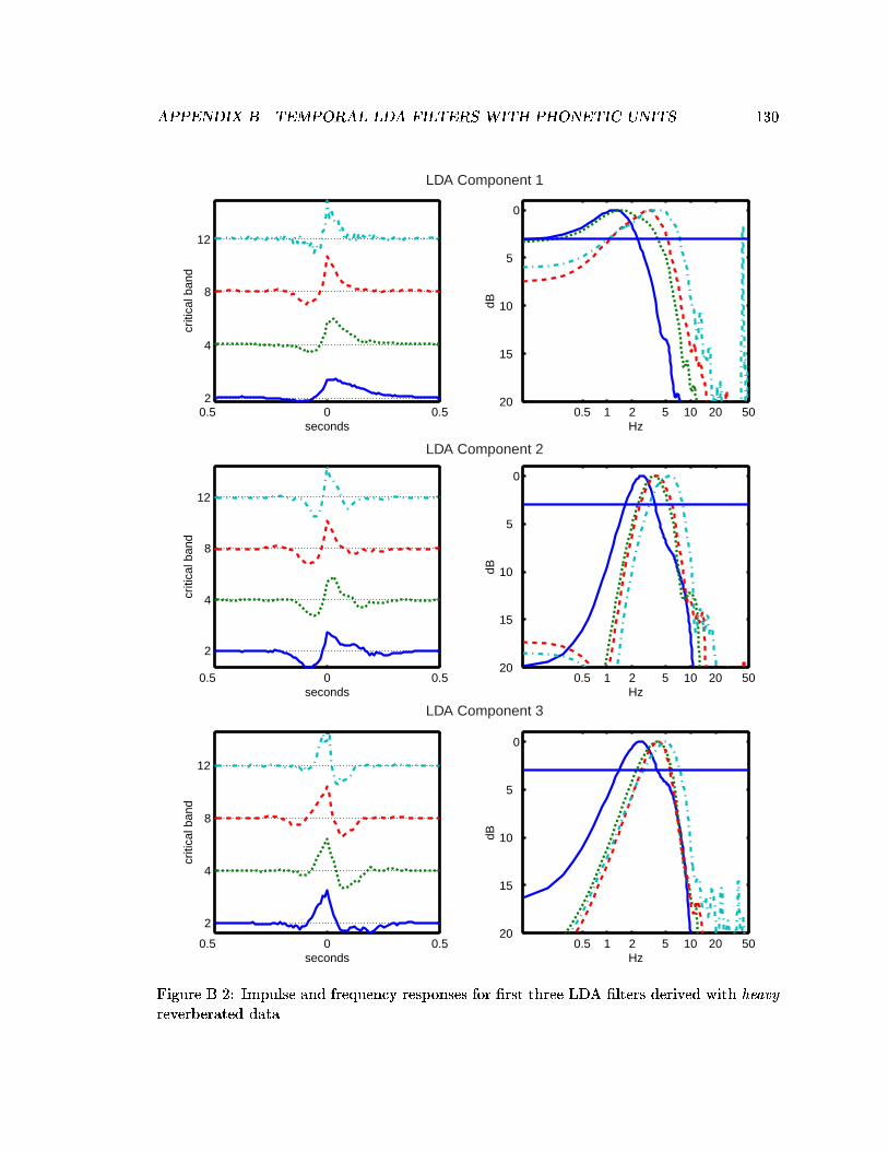
APPENDIX B. TEMPORAL LDA FILTERS WITH PHONETIC UNITS 130
0.5 0 0.5 2
4
8
12
seconds
criti
cal b
and
0.5 1 2 5 10 20 5020
15
10
5
0
Hz
dB
0.5 0 0.5
2
4
8
12
seconds
criti
cal b
and
0.5 1 2 5 10 20 5020
15
10
5
0
Hz
dB
0.5 0 0.5
2
4
8
12
seconds
criti
cal b
and
0.5 1 2 5 10 20 5020
15
10
5
0
Hz
dB
LDA Component 1
LDA Component 2
LDA Component 3
Figure B.2: Impulse and frequency responses for �rst three LDA �lters derived with heavy
reverberated data.
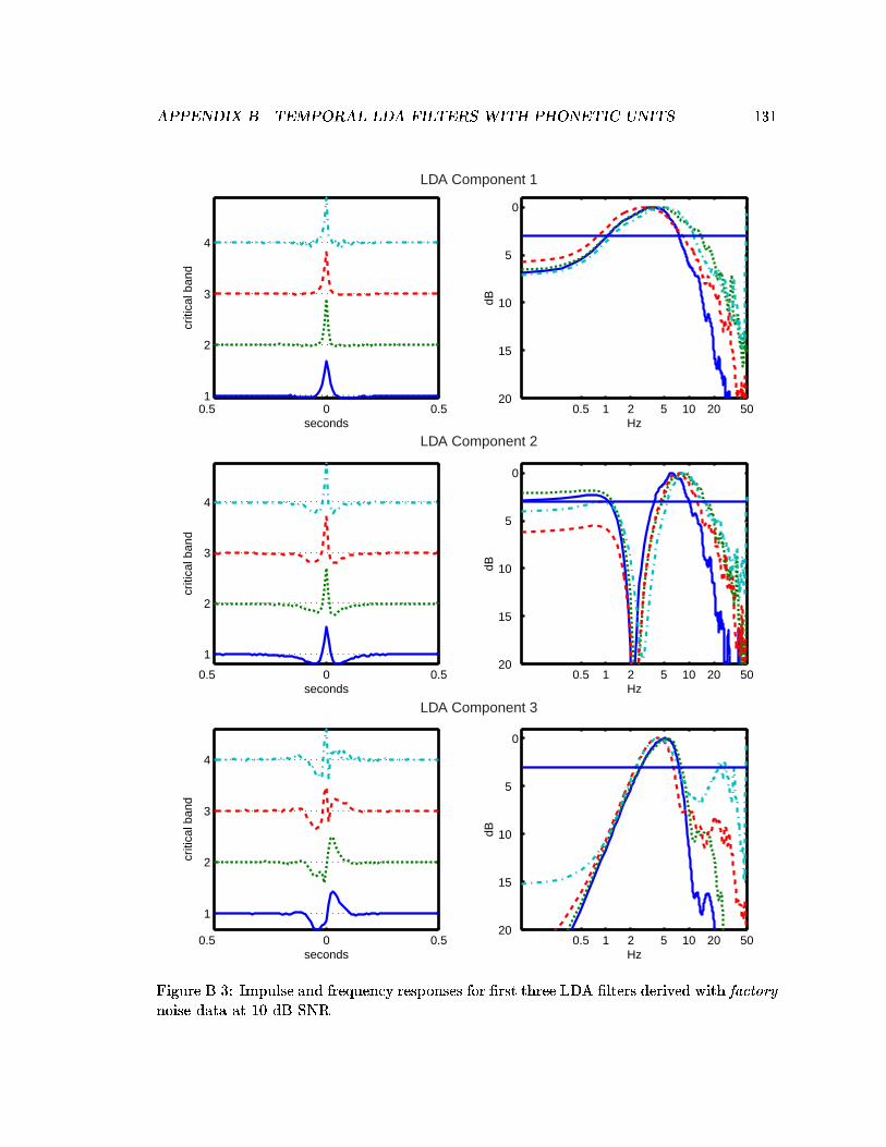
APPENDIX B. TEMPORAL LDA FILTERS WITH PHONETIC UNITS 131
0.5 0 0.5 1
2
3
4
seconds
criti
cal b
and
0.5 1 2 5 10 20 5020
15
10
5
0
Hz
dB
0.5 0 0.5
1
2
3
4
seconds
criti
cal b
and
0.5 1 2 5 10 20 5020
15
10
5
0
Hz
dB
0.5 0 0.5
1
2
3
4
seconds
criti
cal b
and
0.5 1 2 5 10 20 5020
15
10
5
0
Hz
dB
LDA Component 1
LDA Component 2
LDA Component 3
Figure B.3: Impulse and frequency responses for �rst three LDA �lters derived with factorynoise data at 10 dB SNR.
132
Appendix C
Temporal LDA Filters with
Syllabic Units
Since the LDA �lters derived in heavy reverberation tended to restrict the mod-
ulation rates to those commensurate with syllabic rates, pilot tests were conducted using
syllabic targets in lieu of phonetic targets. These syllabic targets were derived from the
phonetic targets using the tsylb program written by Bill Fisher at the National Institute
of Standards and Technology (NIST). The program grouped phone sequences into sylla-
bles using phonotactic and pronunciation rules. When applied to the OGI Stories corpus,
the algorithm produces 5427 distinct syllable patterns, most of which occurred very infre-
quently. For �lter derivation, the 100 most frequent syllable patterns (comprising 42% of
the total number of syllable instances) were used as class targets. Detailed plots of the
three principal LDA �lters derived with these targets with clean data is shown in Figure
C.1. The preferred frequency ranges are consistent with those found in the reverberation
cases using phonetic targets. A comparison of the LDA �lters derived in di�erent noise
conditions using syllable targets is shown in Figure C.2. The frequency responses in this
plot are of the averaged impulse responses across thirteen frequency bands (neglecting the
highest and lowest ones). Whereas phonetic targets yielded band-pass ranges that changed
drastically with reverberation conditions, the �lters using syllable targets were noticeably
consistent. This was also true when using additive noise.
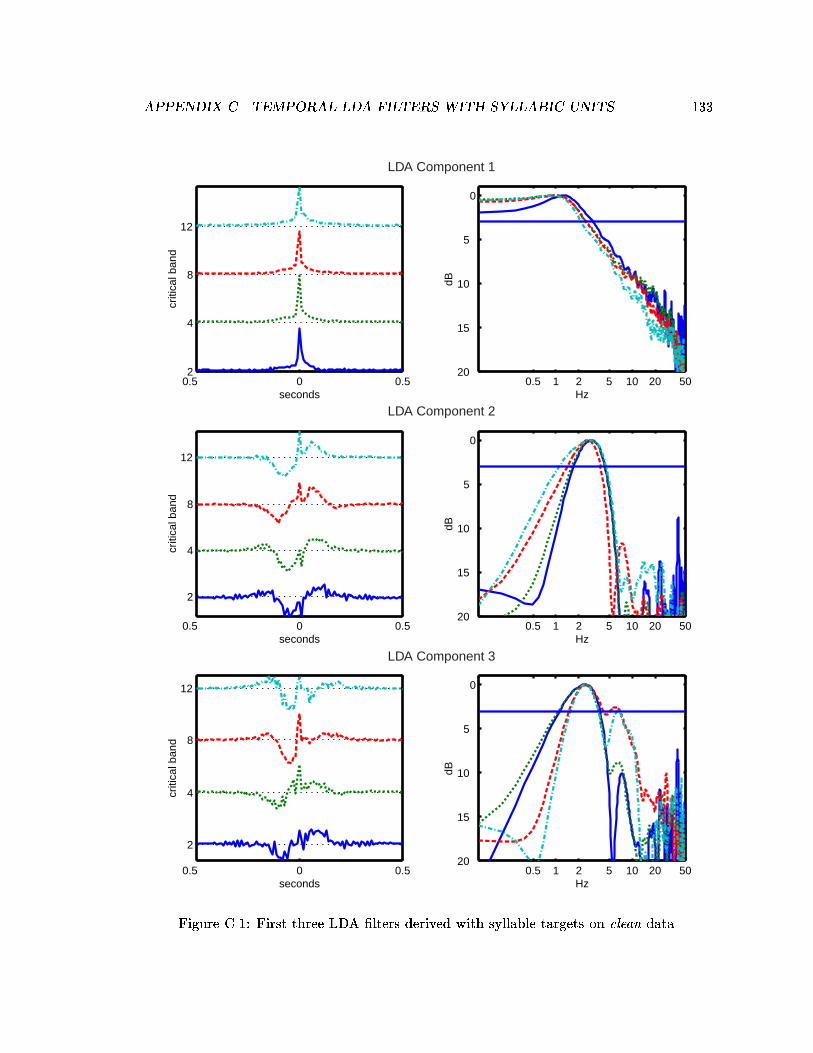
APPENDIX C. TEMPORAL LDA FILTERS WITH SYLLABIC UNITS 133
0.5 0 0.5 2
4
8
12
seconds
criti
cal b
and
0.5 1 2 5 10 20 5020
15
10
5
0
Hz
dB
0.5 0 0.5
2
4
8
12
seconds
criti
cal b
and
0.5 1 2 5 10 20 5020
15
10
5
0
Hz
dB
0.5 0 0.5
2
4
8
12
seconds
criti
cal b
and
0.5 1 2 5 10 20 5020
15
10
5
0
Hz
dB
LDA Component 1
LDA Component 2
LDA Component 3
Figure C.1: First three LDA �lters derived with syllable targets on clean data.
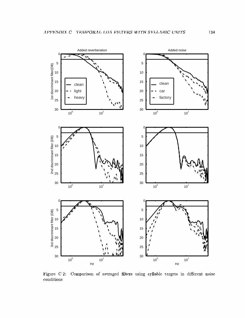
APPENDIX C. TEMPORAL LDA FILTERS WITH SYLLABIC UNITS 134
100
101
30
25
20
15
10
5
0Added reverberation
1st d
iscr
imin
ant f
ilter
(DB
)
100
101
30
25
20
15
10
5
0Added noise
100
101
30
25
20
15
10
5
0
2nd
disc
rimin
ant f
ilter
(D
B)
100
101
30
25
20
15
10
5
0
100
101
30
25
20
15
10
5
0
3rd
disc
rimin
ant f
ilter
(D
B)
Hz10
010
130
25
20
15
10
5
0
Hz
clean
light
heavy
clean
car
factory
Figure C.2: Comparison of averaged �lters using syllable targets in di�erent noiseconditions.
135
Appendix D
Temporal LDA Filters for PLP
LDA �lters derived using PLP cepstral trajectories are shown in �gure D.1. This
plot has impulse and frequency responses from clean data. Only the �rst, fourth, and
seventh of the 8 cepstral coe�cients are plotted for comparison. Since the individual
cepstral components are only weakly correlated there appears to be more di�erences among
the �lter responses of the di�erent cepstral components. Despite the apparent noisiness in
the responses, the �lters do generally maintain a \Mexican-hat" band-pass shape.
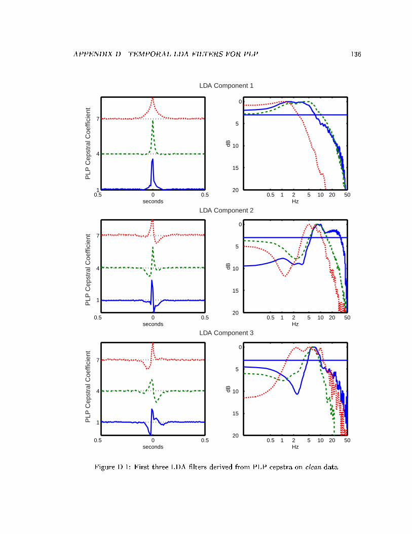
APPENDIX D. TEMPORAL LDA FILTERS FOR PLP 136
0.5 0 0.5 1
4
7
seconds0.5 1 2 5 10 20 50
20
15
10
5
0
Hz
dB
0.5 0 0.5
1
4
7
seconds0.5 1 2 5 10 20 50
20
15
10
5
0
Hz
dB
0.5 0 0.5
1
4
7
seconds0.5 1 2 5 10 20 50
20
15
10
5
0
Hz
dB
LDA Component 1
LDA Component 3
LDA Component 2
PLP
Cep
stra
l Coe
ffici
ent
PLP
Cep
stra
l Coe
ffici
ent
PLP
Cep
stra
l Coe
ffici
ent
Figure D.1: First three LDA �lters derived from PLP cepstra on clean data.
137
Appendix E
Correlating Frame Accuracy and
Word Error
Frame accuracy is a common and natural summary statistic to use in speech
classi�cation tasks. In neural-network-based ASR it is convenient to use such a statistic
when estimating sub-word-unit probabilities in the acoustic modeling stage. For example,
frame accuracy gives an indication of the performance of the MLP probability estimator
and is used for the stopping criterion during training. However, as with many summary
statistics, it presents an incomplete and sometimes de�cient indicator of performance for
the overall task of word recognition. Many of our experiments with LDA temporal �lters,
for example, gave rise to cases where an improvement in the frame accuracy resulted in
either no signi�cant change or an increased word error. This is a problem that has been
seen by many in the ASR community. Unfortunately, we are not aware of any detailed
analysis or satisfactory explanation to comprehensively account for instances when frame
accuracy and word error are uncorrelated. Without such an answer, many are forced to
rationalize or excuse such results to complex interactions in the ASR system, as we have.
We conducted pilot experiments in an e�ort to illustrate some of the variability
in word-recognition performance associated with frame accuracy. This preliminary study
also attempts to shed light on some of the factors that might give rise to instances where
frame accuracy and word error correlate (or not). Some of the results are con�rmation of
intuitive or commonly known trends.
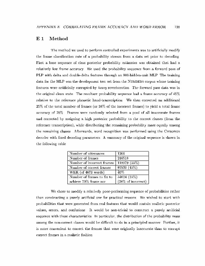
APPENDIX E. CORRELATING FRAME ACCURACY AND WORD ERROR 138
E.1 Method
The method we used to perform controlled experiments was to arti�cially modify
the frame classi�cation rate of a probability stream from a data set prior to decoding.
First a base sequence of class posterior probability estimates was obtained that had a
relatively low frame accuracy. We used the probability sequence from a forward pass of
PLP with delta and double-delta features through an 800-hidden-unit MLP. The training
data for the MLP was the development test set from the Numbers corpus whose training
features were arti�cially corrupted by heavy reverberation. The forward pass data was in
the original clean state. The resultant probability sequence had a frame accuracy of 45%
relative to the reference phonetic hand-transcription. We then corrected an additional
25% of the total number of frames (or 38% of the incorrect frames) to yield a total frame
accuracy of 70%. Frames were randomly selected from a pool of all inaccurate frames
and corrected by assigning a high posterior probability to the correct classes (from the
reference transcription), while distributing the remaining probability mass equally among
the remaining classes. Afterwards, word recognition was performed using the Chronos
decoder with �xed decoding parameters. A summary of the original sequence is shown in
the following table.
Number of utterances 1206
Number of frames 216518
Number of incorrect frames 118979 (55%)
Number of correct frames 97539 (45%)
WER (of 4673 words) ~40%
Number of frames to �x to 54024 (25%)achieve 70% frame acc. (38% of incorrect)
We chose to modify a relatively poor-performing sequence of probabilities rather
than constructing a purely arti�cial one for practical reasons. We wished to start with
probabilities that were generated from real features that would contain realistic posterior
values, errors, and confusions. It would be non-trivial to construct a purely arti�cial
sequence with these characteristics. In particular, the distribution of the probability mass
among the non-correct classes would be di�cult to do in a principled manner. Further, it
is more convenient to correct the frames that were originally inaccurate than to corrupt
correct frames in a realistic fashion.
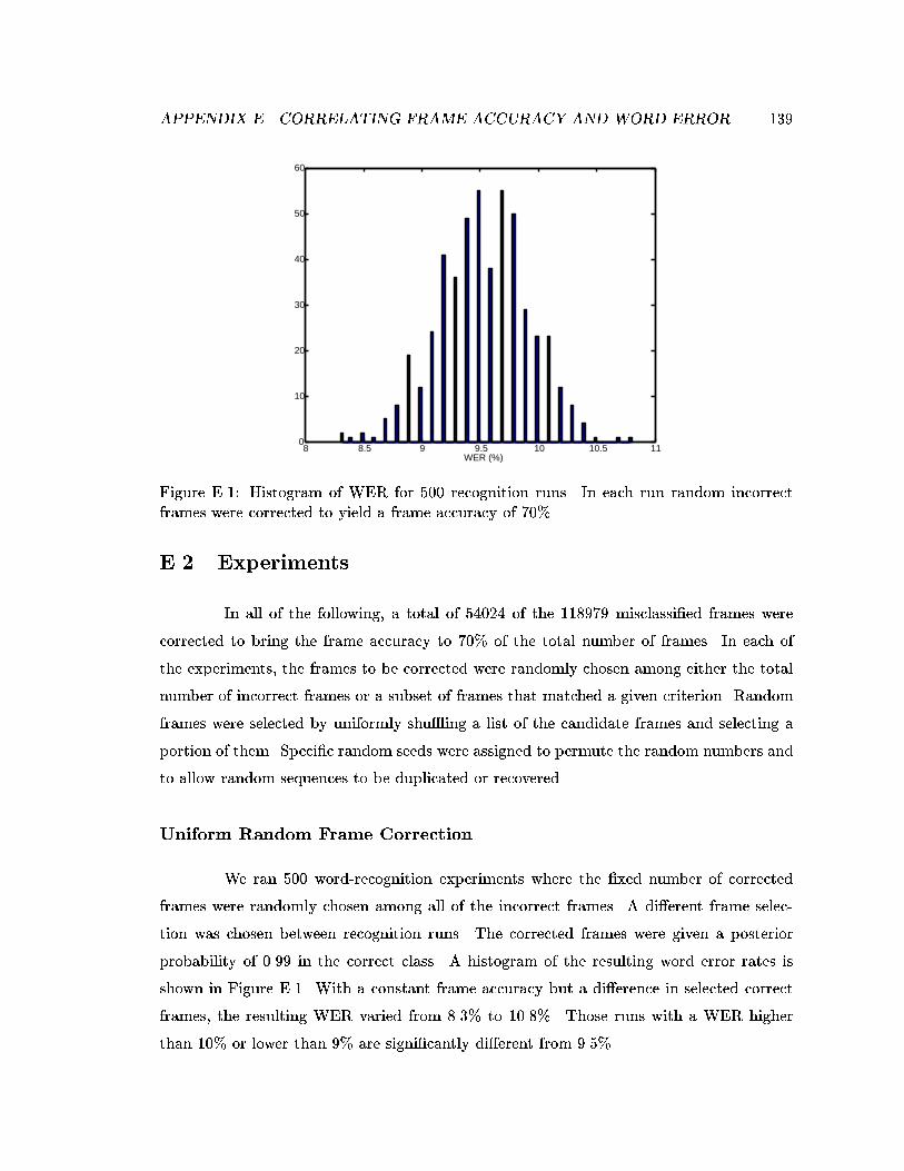
APPENDIX E. CORRELATING FRAME ACCURACY AND WORD ERROR 139
8 8.5 9 9.5 10 10.5 110
10
20
30
40
50
60
WER (%)
Figure E.1: Histogram of WER for 500 recognition runs. In each run random incorrectframes were corrected to yield a frame accuracy of 70%.
E.2 Experiments
In all of the following, a total of 54024 of the 118979 misclassi�ed frames were
corrected to bring the frame accuracy to 70% of the total number of frames. In each of
the experiments, the frames to be corrected were randomly chosen among either the total
number of incorrect frames or a subset of frames that matched a given criterion. Random
frames were selected by uniformly shu�ing a list of the candidate frames and selecting a
portion of them. Speci�c random seeds were assigned to permute the random numbers and
to allow random sequences to be duplicated or recovered.
Uniform Random Frame Correction
We ran 500 word-recognition experiments where the �xed number of corrected
frames were randomly chosen among all of the incorrect frames. A di�erent frame selec-
tion was chosen between recognition runs. The corrected frames were given a posterior
probability of 0.99 in the correct class. A histogram of the resulting word error rates is
shown in Figure E.1. With a constant frame accuracy but a di�erence in selected correct
frames, the resulting WER varied from 8.3% to 10.8%. Those runs with a WER higher
than 10% or lower than 9% are signi�cantly di�erent from 9.5%.
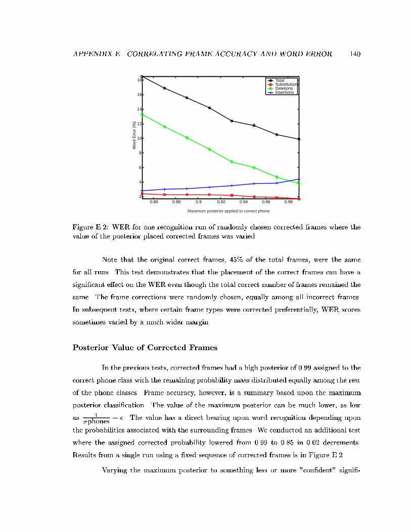
APPENDIX E. CORRELATING FRAME ACCURACY AND WORD ERROR 140
0.86 0.88 0.9 0.92 0.94 0.96 0.982
4
6
8
10
12
14
16
18
Wor
d E
rror
(%
)
Total SubstitutionsDeletions Insertions
Maximum posterior applied to correct phone
Figure E.2: WER for one recognition run of randomly chosen corrected frames where thevalue of the posterior placed corrected frames was varied.
Note that the original correct frames, 45% of the total frames, were the same
for all runs. This test demonstrates that the placement of the correct frames can have a
signi�cant e�ect on the WER even though the total correct number of frames remained the
same. The frame corrections were randomly chosen, equally among all incorrect frames.
In subsequent tests, where certain frame types were corrected preferentially, WER scores
sometimes varied by a much wider margin.
Posterior Value of Corrected Frames
In the previous tests, corrected frames had a high posterior of 0.99 assigned to the
correct phone class with the remaining probability mass distributed equally among the rest
of the phone classes. Frame accuracy, however, is a summary based upon the maximum
posterior classi�cation. The value of the maximum posterior can be much lower, as low
as 1#phones + �. The value has a direct bearing upon word recognition depending upon
the probabilities associated with the surrounding frames. We conducted an additional test
where the assigned corrected probability lowered from 0.99 to 0.85 in 0.02 decrements.
Results from a single run using a �xed sequence of corrected frames is in Figure E.2.
Varying the maximum posterior to something less or more "con�dent" signi�-
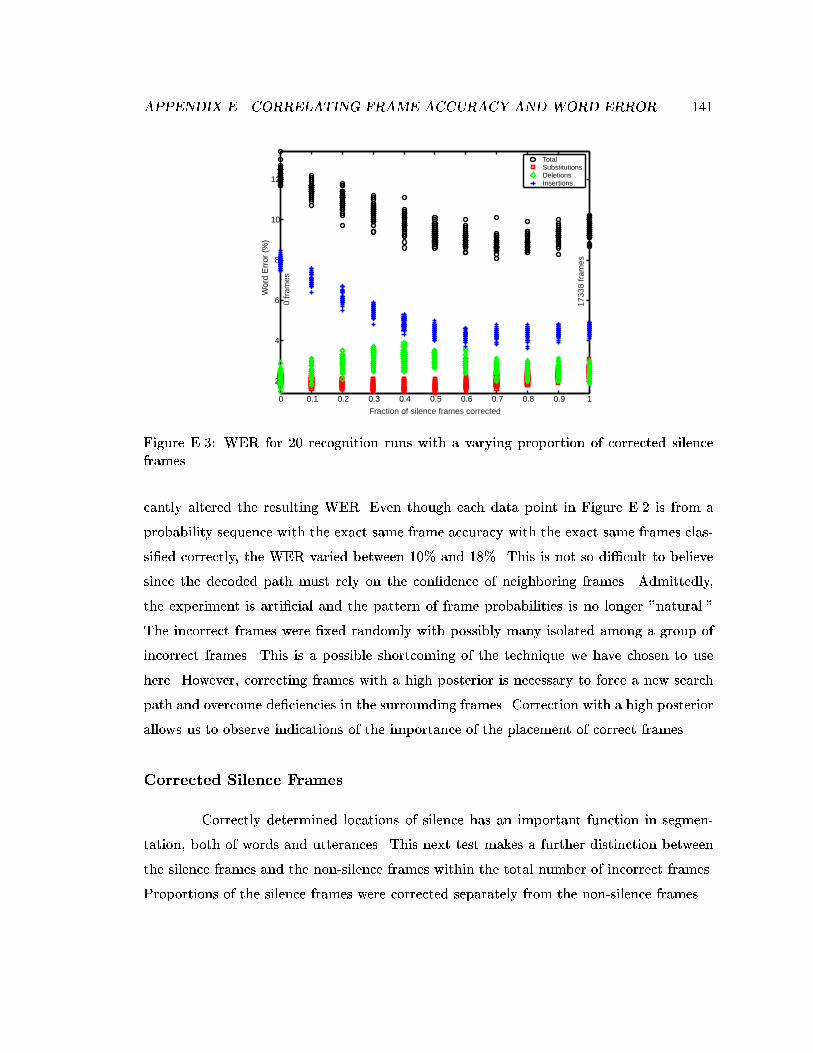
APPENDIX E. CORRELATING FRAME ACCURACY AND WORD ERROR 141
0 0.1 0.2 0.3 0.4 0.5 0.6 0.7 0.8 0.9 1
2
4
6
8
10
12
Wor
d E
rror
(%
)
Total SubstitutionsDeletions Insertions
Fraction of silence frames corrected
1733
8 fr
ames
0 fr
ames
Figure E.3: WER for 20 recognition runs with a varying proportion of corrected silenceframes.
cantly altered the resulting WER. Even though each data point in Figure E.2 is from a
probability sequence with the exact same frame accuracy with the exact same frames clas-
si�ed correctly, the WER varied between 10% and 18%. This is not so di�cult to believe
since the decoded path must rely on the con�dence of neighboring frames. Admittedly,
the experiment is arti�cial and the pattern of frame probabilities is no longer "natural."
The incorrect frames were �xed randomly with possibly many isolated among a group of
incorrect frames. This is a possible shortcoming of the technique we have chosen to use
here. However, correcting frames with a high posterior is necessary to force a new search
path and overcome de�ciencies in the surrounding frames. Correction with a high posterior
allows us to observe indications of the importance of the placement of correct frames.
Corrected Silence Frames
Correctly determined locations of silence has an important function in segmen-
tation, both of words and utterances. This next test makes a further distinction between
the silence frames and the non-silence frames within the total number of incorrect frames.
Proportions of the silence frames were corrected separately from the non-silence frames.
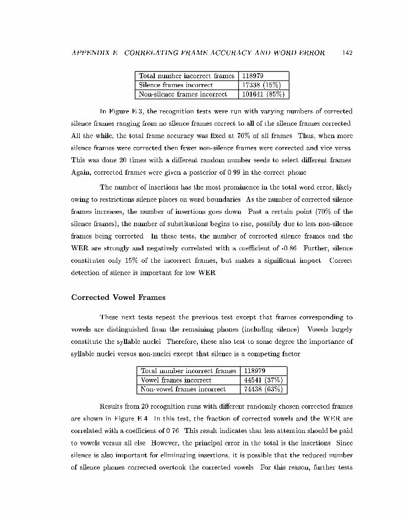
APPENDIX E. CORRELATING FRAME ACCURACY AND WORD ERROR 142
Total number incorrect frames 118979
Silence frames incorrect 17338 (15%)
Non-silence frames incorrect 101641 (85%)
In Figure E.3, the recognition tests were run with varying numbers of corrected
silence frames ranging from no silence frames correct to all of the silence frames corrected.
All the while, the total frame accuracy was �xed at 70% of all frames. Thus, when more
silence frames were corrected then fewer non-silence frames were corrected and vice versa.
This was done 20 times with a di�erent random number seeds to select di�erent frames.
Again, corrected frames were given a posterior of 0.99 in the correct phone.
The number of insertions has the most prominence in the total word error, likely
owing to restrictions silence places on word boundaries. As the number of corrected silence
frames increases, the number of insertions goes down. Past a certain point (70% of the
silence frames), the number of substitutions begins to rise, possibly due to less non-silence
frames being corrected. In these tests, the number of corrected silence frames and the
WER are strongly and negatively correlated with a coe�cient of -0.86. Further, silence
constitutes only 15% of the incorrect frames, but makes a signi�cant impact. Correct
detection of silence is important for low WER.
Corrected Vowel Frames
These next tests repeat the previous test except that frames corresponding to
vowels are distinguished from the remaining phones (including silence). Vowels largely
constitute the syllable nuclei. Therefore, these also test to some degree the importance of
syllable nuclei versus non-nuclei except that silence is a competing factor.
Total number incorrect frames 118979
Vowel frames incorrect 44541 (37%)
Non-vowel frames incorrect 74438 (63%)
Results from 20 recognition runs with di�erent randomly chosen corrected frames
are shown in Figure E.4. In this test, the fraction of corrected vowels and the WER are
correlated with a coe�cient of 0.76. This result indicates that less attention should be paid
to vowels versus all else. However, the principal error in the total is the insertions. Since
silence is also important for eliminating insertions, it is possible that the reduced number
of silence phones corrected overtook the corrected vowels. For this reason, further tests
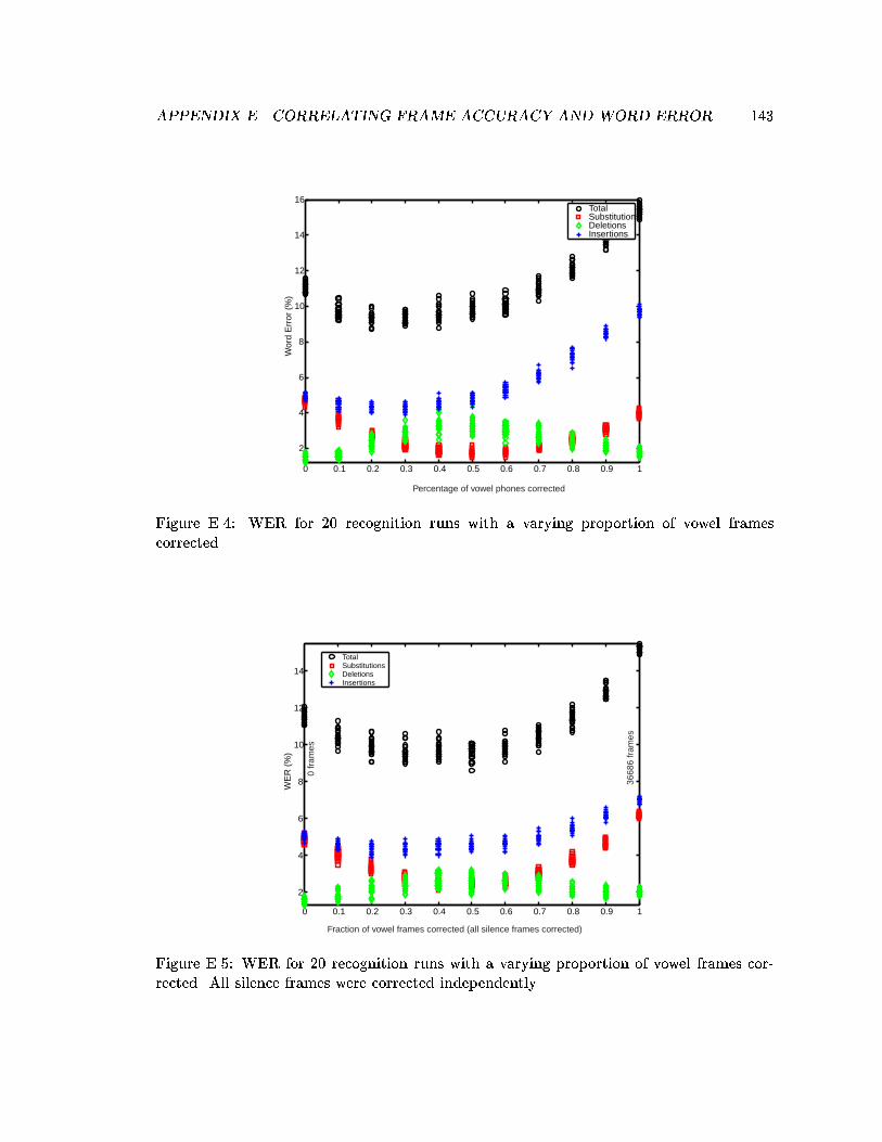
APPENDIX E. CORRELATING FRAME ACCURACY AND WORD ERROR 143
0 0.1 0.2 0.3 0.4 0.5 0.6 0.7 0.8 0.9 1
2
4
6
8
10
12
14
16
Wor
d E
rror
(%
)
Total SubstitutionsDeletions Insertions
Percentage of vowel phones corrected
Figure E.4: WER for 20 recognition runs with a varying proportion of vowel framescorrected.
0 0.1 0.2 0.3 0.4 0.5 0.6 0.7 0.8 0.9 1
2
4
6
8
10
12
14
WE
R (
%)
Total SubstitutionsDeletions Insertions
Fraction of vowel frames corrected (all silence frames corrected)
3668
6 fr
ames
0 fr
ames
Figure E.5: WER for 20 recognition runs with a varying proportion of vowel frames cor-rected. All silence frames were corrected independently.
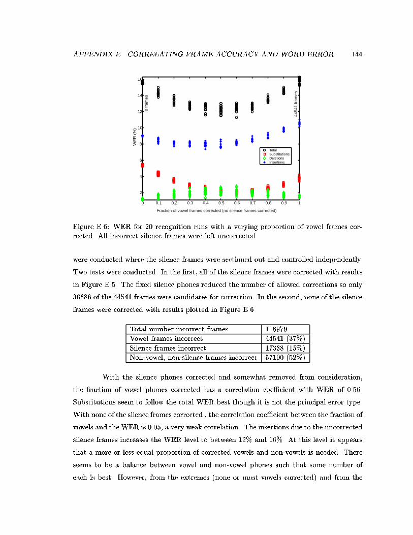
APPENDIX E. CORRELATING FRAME ACCURACY AND WORD ERROR 144
0 0.1 0.2 0.3 0.4 0.5 0.6 0.7 0.8 0.9 1
2
4
6
8
10
12
14
16
WE
R (
%)
Total SubstitutionsDeletions Insertions
Fraction of vowel frames corrected (no silence frames corrected)
4454
1 fr
ames
0 fr
ames
Figure E.6: WER for 20 recognition runs with a varying proportion of vowel frames cor-rected. All incorrect silence frames were left uncorrected.
were conducted where the silence frames were sectioned out and controlled independently.
Two tests were conducted. In the �rst, all of the silence frames were corrected with results
in Figure E.5. The �xed silence phones reduced the number of allowed corrections so only
36686 of the 44541 frames were candidates for correction. In the second, none of the silence
frames were corrected with results plotted in Figure E.6.
Total number incorrect frames 118979
Vowel frames incorrect 44541 (37%)
Silence frames incorrect 17338 (15%)
Non-vowel, non-silence frames incorrect 57100 (52%)
With the silence phones corrected and somewhat removed from consideration,
the fraction of vowel phones corrected has a correlation coe�cient with WER of 0.56.
Substitutions seem to follow the total WER best though it is not the principal error type.
With none of the silence frames corrected , the correlation coe�cient between the fraction of
vowels and the WER is 0.05, a very weak correlation. The insertions due to the uncorrected
silence frames increases the WER level to between 12% and 16%. At this level it appears
that a more or less equal proportion of corrected vowels and non-vowels is needed. There
seems to be a balance between vowel and non-vowel phones such that some number of
each is best. However, from the extremes (none or most vowels corrected) and from the
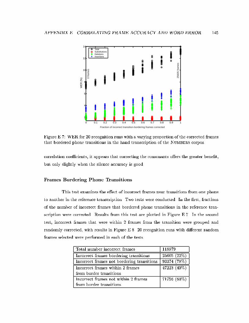
APPENDIX E. CORRELATING FRAME ACCURACY AND WORD ERROR 145
0 0.1 0.2 0.3 0.4 0.5 0.6 0.7 0.8 0.9 1
2
4
6
8
10
12
14
WE
R (
%)
Total SubstitutionsDeletions Insertions
Fraction of incorrect transition-bordering frames corrected
2560
5 fr
ames
0 fr
ames
Figure E.7: WER for 20 recognition runs with a varying proportion of the corrected framesthat bordered phone transitions in the hand transcription of the Numbers corpus.
correlation coe�cients, it appears that correcting the consonants o�ers the greater bene�t,
but only slightly when the silence accuracy is good.
Frames Bordering Phone Transitions
This test examines the e�ect of incorrect frames near transitions from one phone
to another in the reference transcription. Two tests were conducted. In the �rst, fractions
of the number of incorrect frames that bordered phone transitions in the reference tran-
scription were corrected. Results from this test are plotted in Figure E.7. In the second
test, incorrect frames that were within 2 frames from the transition were grouped and
randomly corrected, with results in Figure E.8. 20 recognition runs with di�erent random
frames selected were performed in each of the tests.
Total number incorrect frames 118979
Incorrect frames bordering transitions 25605 (22%)
Incorrect frames not bordering transitions 93374 (78%)
Incorrect frames within 2 frames 47223 (40%)from border transitions
Incorrect frames not within 2 frames 71756 (60%)from border transitions
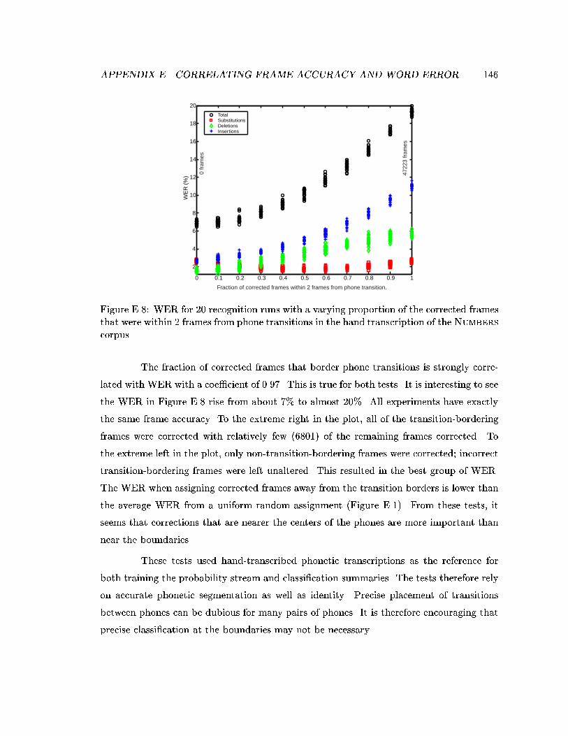
APPENDIX E. CORRELATING FRAME ACCURACY AND WORD ERROR 146
0 0.1 0.2 0.3 0.4 0.5 0.6 0.7 0.8 0.9 1
2
4
6
8
10
12
14
16
18
20
WE
R (
%)
Total SubstitutionsDeletions Insertions
Fraction of corrected frames within 2 frames from phone transition.
4722
3 fr
ames
0 fr
ames
Figure E.8: WER for 20 recognition runs with a varying proportion of the corrected framesthat were within 2 frames from phone transitions in the hand transcription of the Numberscorpus.
The fraction of corrected frames that border phone transitions is strongly corre-
lated with WER with a coe�cient of 0.97. This is true for both tests. It is interesting to see
the WER in Figure E.8 rise from about 7% to almost 20%. All experiments have exactly
the same frame accuracy. To the extreme right in the plot, all of the transition-bordering
frames were corrected with relatively few (6801) of the remaining frames corrected. To
the extreme left in the plot, only non-transition-bordering frames were corrected; incorrect
transition-bordering frames were left unaltered. This resulted in the best group of WER.
The WER when assigning corrected frames away from the transition borders is lower than
the average WER from a uniform random assignment (Figure E.1). From these tests, it
seems that corrections that are nearer the centers of the phones are more important than
near the boundaries.
These tests used hand-transcribed phonetic transcriptions as the reference for
both training the probability stream and classi�cation summaries. The tests therefore rely
on accurate phonetic segmentation as well as identity. Precise placement of transitions
between phones can be dubious for many pairs of phones. It is therefore encouraging that
precise classi�cation at the boundaries may not be necessary.
APPENDIX E. CORRELATING FRAME ACCURACY AND WORD ERROR 147
E.3 Discussion
Word recognition error depends upon the accurate classi�cation of the frame
probabilities, the locations of the errors and the frame posterior values. A random sampling
of corrected frames gives rise to a distribution of corresponding word error rates despite
equal overall frame accuracy. Varying the proportion of some types of frame errors can
yield results that vary in a systematic fashion. Depending upon the proportion of errors,
the resulting WER can vary by a signi�cant amount. With these complications, the frame
accuracy is not necessarily a proper measure when comparing the acoustic probabilities
of two or more streams. Since the value of the maximum posterior can have a strong
e�ect on WER, we also considered a frame accuracy weighted by the posterior values
for the correct class and an average of the posteriors for the correct classes. Computed
measures were, however, only weakly correlated with WER, with a coe�cient of -0.10.
Additional weighting could be included if it is determined that certain types of frames are
more important than others in the resulting decoding. For example, the silence frames
are relatively important whereas the transition bordering frames may not be. Naturally,
further tests are needed for a better picture.
A thorough investigation of the relationship between frame accuracy and word
recognition would require a more detailed sensitivity analysis of the decoding system and
the models. Such an analysis is non-trivial to construct and is dependent upon the decoding
algorithm and its parameters. The random selection approach conducted here is a general
empirical method that is independent of the speci�c decoder and can yield some indication
as to factors that are important for word recognition. Our tests examined to some degree
the location of frame errors depending on criteria such as silence, vowel and phone tran-
sition. Further tests associated with model states can be conducted with other decoders
that provide decoding lattice information. The results may be combined and compared to
related work by Chang et. al. who analyzed frame errors relative to phone position [21]
and Greenberg et. al. who conducted ASR diagnostic evaluations with respect to many
acoustic, linguistic and speaker characteristics [42, 41]. As this topic is tangential to this
thesis, such a pursuit is left to future investigations. Results from future diagnostics may
aid in selecting and training front-end acoustic modeling in a manner better suited to the
overall goal of word recognition.
148
Bibliography
[1] Fevzi Alimoglu and Etham Aplaydin. Combining multiple representations and clas-
si�ers for pen-based handwritten digit recognition. In Proceedings of the Fourth
International Conference on Document Analysis and Recognition, volume 2, pages
637{40, Ulm, Germany, August 1997.
[2] Jont B. Allen. How do humans process and recognize speech? IEEE Transactions
on Speech and Audio Processing, 2(4):567{77, October 1994.
[3] Christos Antoniou and Je� Reynolds. Acoustic modelling using modular/ensemble
combinations of heterogeneous neural networks. In International Conference on Spo-
ken Language Processing, volume 1, pages 282{5, Beijing, China, October 2000.
[4] Takayuki Arai and Steven Greenberg. Speech intelligibility in the presence of cross-
channel spectral asynchrony. In International Conference on Acoustics Speech and
Signal Processing, volume 2, pages 933{6, Seattle, Washington, May 1998. IEEE.
[5] Takayuki Arai, Misha Pavel, Hynek Hermansky, and Carlos Avendano. Syllable
intelligibility for temporally �ltered lpc cepstral trajectories. J. Acoust. Soc. Am.,
105(5):2783{91, May 1999.
[6] Carlos Avendano, Sarel van Vuuren, and Hynek Hermansky. Data based �lter de-
sign for RASTA-like channel normalization in ASR. In International Conference on
Spoken Language Processing, volume 3, pages 2087{90, Philadephia, Pennsylvania,
October 1996.
[7] Je� A. Bilmes. Joint distributional modeling with cross-correlation based features. In
Proc. IEEE Automatic Speech Recognition and Understanding, pages 148{55, Santa
Barbara, California, December 1997.
BIBLIOGRAPHY 149
[8] Je� A. Bilmes and Katrin Kirchho�. Directed graphical models of classi�er combi-
nations: application to phone recognition. In International Conference on Spoken
Language Processing, volume 3, pages 921{4, Beijing, China, October 2000.
[9] B. Bogert, M. Healy, and J. Tukey. The quefrency analysis of time series for echos. In
M. Rosenblatt, editor, Proc. Symposium on Time Series Analysis, chapter 15, pages
209{43. Wiley, New York, 1963.
[10] Herv�e Bourlard and St�ephane Dupont. A new ASR approach based on independent
processing and recombination of partial frequency bands. In International Conference
on Spoken Language Processing, volume 1, pages 426{9, Philadephia, Pennsylvania,
October 1996.
[11] Herv�e Bourlard and St�ephane Dupont. Sub-band based speech recognition. In In-
ternational Conference on Acoustics Speech and Signal Processing, volume 2, pages
1251{4, Munich, Germany, April 1997. IEEE.
[12] Herv�e Bourlard and Nelson Morgan. Connectionist Speech Recognition- A Hybrid
Approach. Kluwer Academic Press, 1994.
[13] Christoph Bregler, Herman Hild, Stephan Manke, and Alex Waibel. Improving con-
nected letter recognition by lipreading. In International Conference on Acoustics
Speech and Signal Processing, volume 1, pages 557{60, Minneapolis, Minnisota, April
1993.
[14] Christoph Bregler and Yochai Konig. "Eigenlips" for robust speech recognition. In
International Conference on Acoustics Speech and Signal Processing, volume 2, pages
669{72, Adelaide, SA, Australia, April 1994. IEEE.
[15] Christoph Bregler, Stephan Manke, Herman Hild, and Alex Waibel. Bimodal sensor
integration on the example of 'speechreading'. In International Conference on Neural
Networks, volume 2, pages 667{71, San Francisco, California, March 1993. IEEE.
[16] Christoph Bregler, Stephen M. Omohundro, and Yochai Konig. A hybrid approach
to bimodal speech recognition. In Conference Record of the Twenty-Eighth Asilomar
Conference on Signals, Systems and Computers, volume 1, pages 556{60, Paci�c
Grove, California, October 1994.
BIBLIOGRAPHY 150
[17] John S. Bridle. Probabilistic interpretation of feedforward classi�cation network out-
puts, with relationship to statistical pattern recognition. In F. Fogelman Soulie and
J. He'roult, editors, Neurocomputing: Algorithms, Architectures, and Applications,
pages 227{36. Springer Verlag, New York, 1990.
[18] Pierre J. Castellano, Stefan Slomka, and Sridha Sridharan. Telephone based speaker
recognition using multiple binary classi�er and Gaussian mixture models. In In-
ternational Conference on Acoustics Speech and Signal Processing, volume 1, pages
1075{8, Munich, Germany, April 1997. IEEE.
[19] Center for Spoken Language Understanding, Department of Computer Science and
Engineering, Oregon Graduate Institute. Numbers corpus, release 1.0, 1995.
[20] Center for Spoken Language Understanding, Department of Computer Science and
Engineering, Oregon Graduate Institute. OGI multi-lingual corpus, 1994.
[21] Shuangyu Chang, Lokendra Shastri, and Steven Greenberg. Automatic phonetic
transcription of spontaneous speech (american english). In International Conference
on Acoustics Speech and Signal Processing, volume 4, pages 330{3, Beijing, China,
October 2000.
[22] Michael M. Cohen and Dominic W. Massaro. What can visual speech synthesis tell
visual speech recognition? In Conference Record of the Twenty-Eighth Asilomar
Conference on Signals, Systems and Computers, volume 1, pages 566{71, Paci�c
Grove, California, October 1994.
[23] Thomas M. Cover and Joy A. Thomas. Elements of Information Theory. Wiley, New
York, 1991.
[24] Steven B. Davis and Paul Mermelstein. Comparison of parametric representations for
monosyllabic word recognition in continuously spoken sentences. IEEE Transactions
on Acoustics, Speech and Signal Processing, 28(4):357{366, August 1980.
[25] A. P. Dempster, N. M. Laird, and D .B. Rubin. Maximum-likelihood from incomplete
data via the EM algorithm. Journal of the Royal Statistical Society Series B, (39):1{
38, 1977.
BIBLIOGRAPHY 151
[26] Rob Drullman. Temporal envelope and �ne structure cues for speech intelligibility.
Journal of the Acoustical Society of America, 97(1):585{592, January 1995.
[27] Rob Drullman, Joost M. Feston, and Reinier Plomp. E�ect of temporal enve-
lope smearing on speech reception. Journal of the Acoustic Society of America,
95(2):1053{64, February 1994.
[28] Richard O. Duda and Peter E. Hart. Pattern Classi�cation and Scene Analysis. John
Wiley & Sons, 1973.
[29] H. Dudley, R. Riesz, and S. Watkins. A synthetic speaker. Journal of the Franklin
Institute, (227):739, 1939.
[30] Daniel P. W. Ellis and Je� A. Bilmes. Using mutual information to design feature
combinations. In International Conference on Spoken Language Processing, volume 3,
pages 79{82, Beijing, China, October 2000.
[31] J. G. Fiscus. A post-processing system to yield reduced word error rates: Recognizer
output voting error reduction (ROVER). In IEEE Workshop on Automatic Speech
Recognition and Understanding, pages 347{54, 1997.
[32] James L. Flanagan. Speech Analysis Synthesis and Perception. Springer-Verlag, New
York/Berlin, 2 edition, 1972.
[33] Harvey Fletcher. Speech and Hearing in Communication. Krieger, New York, 1953.
[34] J�urgen Fritsch, Michael Finke, and Alex Waibel. Adaptively growing heirarchical
mixtures of experts. In Advances in Neural Information Processing Systems 9, pages
459{65, Denver, Colorado, December 1994.
[35] Keinosuke Fukunaga. Introduction to Satistical Pattern Recognition. Academic Press,
Inc., London, 1990.
[36] Sadaoki Furui. Speaker independent isolated word recognition using dynamic features
of speech spectrum. IEEE Transaction on Acoustics Speech and Signal Processing,
(ASSP-34):52, 1986.
[37] Steven Greenberg. Auditory function. In Malcolm J. Crocker, editor, Encyclopedia
of Acoustics, pages 1301{23. John Wiley, New York, 1997.
BIBLIOGRAPHY 152
[38] Steven Greenberg. The signi�cance of the cochlear travelling wave for theoriesof
frequency analysis and pitch. In E. R. Lewis and C. Steele, editors, Diversity of
Auditory Mechanics. World Scienti�c Press, Singapore, 1997.
[39] Steven Greenberg. Speaking in shorthand - A syllable-centric perspective for under-
standing pronunciation variation. In Proceedings of the ESCA Workshop on Modeling
Pronunciation Variation for Automatic Speech Recognition, Kekrade, United King-
dom, May 1998. ESCA.
[40] Steven Greenberg, Takayuki Arai, and Rosaria Silipo. Speech intelligibility derived
from exceedingly sparse spectral information. In International Conference on Spoken
Language Processing, Sydney, Australia, November 1998.
[41] Steven Greenberg and Shuangyu Chang. Linguistic dissection of switchboard-corpus
automatic speech recognition systems. In Proceedings of the ISCA Workshop on
Automatic Speech Recognition: Challenges for the New Millennium. ICSA, Paris,
France, 2000.
[42] Steven Greenberg, Shuangyu Chang, and Joy Hollenback. An introduction to the
diagnostic evaluation of Switchboard-corpus automatic speech recognition systems.
In Proceedings of the NIST Speech Transcription Workshop, College Park, Maryland,
May 2000.
[43] Steven Greenberg and Brian E. D. Kingsbury. The modulation spectrogram: In
pursuit of an invariant representation of speech. In International Conference on
Acoustics Speech and Signal Processing, volume 3, pages 1647{50, Munich, Germany,
April 1997. IEEE.
[44] Steven Greenberg and Michael L. Shire. Temporal factors in speech perception. In
CSRE-based Teaching Modules for Courses in Speech and Hearing Sciences, pages
91{106. AVAAZ Innovations, London, Ontario, 1997.
[45] Donald D. Greenwood. Critical bandwidth and the frequency coordinates of the
basilar membrane. JASA, 33:1344{1356, 1961.
[46] John H. L. Hansen and Oscar N. Bria. Lombard e�ect compensation for robust auto-
matic speech recognition in noise. In International Conference on Spoken Language
BIBLIOGRAPHY 153
Processing, volume 1, pages 1125{8, Kobe, November 1990. The Acoustical Society
of Japan.
[47] Brian A. Hanson and Ted H. Applebaum. Robust speaker-independent word recogni-
tion using static, dynamic and acceleration features: Experiments with Lombard and
noisy speech. In International Conference on Acoustics Speech and Signal Processing,
volume 2, pages 857{60, Albuquerque, NM, April 1990. IEEE.
[48] Hynek Hermansky. Perceptual linear predictive (PLP) analysis of speech. Journal of
the Acoustical Society of America, 87(4):1738{1752, April 1990.
[49] Hynek Hermansky. The modulation spectrum in the automatic recognition of speech.
In IEEE Workshop on Automatic Speech Recognition and Understanding Proceedings,
pages 140{7, Santa Barbara, CA, USA, December 1997. IEEE Signal Processing
Society.
[50] Hynek Hermansky and Nelson Morgan. RASTA processing of speech. IEEE Trans-
actions on Speech and Audio Processing, 2(4):578{589, October 1994.
[51] Hynek Hermansky and Sangita Sharma. TRAPS - classi�ers for temporal patterns.
In International Conference on Spoken Language Processing, volume 1, pages 193{7,
Sydney, Australia, November 1998.
[52] Hynek Hermansky, Sangita Tibrewala, and Misha Pavel. Towards ASR on partially
corrupted speech. In International Conference on Spoken Language Processing, vol-
ume 1, pages 462{5, Philadephia, Pennsylvania, October 1996.
[53] Kai H�ubener. Using multi-level segmentation coe�cients to improve HMM speech
recognition. In International Conference on Spoken Language Processing, volume 1,
pages 248{51, Philadephia, Pennsylvania, October 1996.
[54] Adam Janin. Multi-stream speech recognition: Ready for prime time? In EU-
ROSPEECH, pages 591{4, Budapest, Hungary, September 1999. ESCA.
[55] Brian E. D. Kingsbury John Wawrzynek, Krste Asanovic and Jim Beck. Spert-ii: A
vector microprocessor system and its applications. InAdvances in Neural Information
Processing Systems 8, pages 619{25, Denver, Colorado, November 1995.
BIBLIOGRAPHY 154
[56] M. I. Jordan and R. A. Jacobs. Heirarchical mixtures of experts and the EM algo-
rithm. Neural Computation, 6(2):181{214, March 1994.
[57] Jean-Claude Junqua, Steven Fincke, and Ken Field. The Lombard e�ect: a re ex to
better communicate with others in noise. In International Conference on Acoustics
Speech and Signal Processing, volume 4, pages 2083{6, Phoenix, AZ, May 1999. IEEE.
[58] Noboru Kanedera, Takayuki Arai, Hynek Hermansky, and Misha Pavel. On the
importance of modulation frequencies for speech recognition. In EUROSPEECH,
volume 3, pages 1079{82, Rhodes, Greece, September 1997. ESCA.
[59] Noboru Kanedera, Takayuki Arai, Hynek Hermansky, and Misha Pavel. On the
relative importance of various components of the modulation spectrum for automatic
speech recognition. Speech Communication, 28:43{55, 1999.
[60] Brian E. D. Kingsbury. Perceptually Inspired Signal-Processing Strategies for Robust
Speech Recognition in Reverberant Environments. PhD thesis, University of California
at Berkeley, 1998.
[61] Brian E. D. Kingsbury and Nelson Morgan. Recognizing reverberant speech with
RASTA-PLP. In International Conference on Acoustics Speech and Signal Process-
ing, volume 2, pages 1259{62, Munich, Germany, April 1997. IEEE.
[62] Brian E. D. Kinsgbury, Nelson Morgan, and Steven Greenberg. Robust speech recog-
nition using the modulation spectrogram. Speech Communication, 25(1-3):117{32,
August 1998.
[63] Katrin Kirchho�. Combining articulatory and acoustic information for speech recog-
nition in noisy and reverberant environments. In International Conference on Spoken
Language Processing, volume 1, pages 186{9, Sydney, Australia, November 1998.
[64] Katrin Kirchho�. Robust Speech Recognition Using Articulatory Information. PhD
thesis, Universit�at Bielefeld, 1999.
[65] Katrin Kirchho� and Je� A. Bilmes. Dynamic classi�er combination in hybrid speech
recognition systems using utterance-level con�dence values. In International Con-
ference on Acoustics Speech and Signal Processing, volume 2, pages 693{6, Phoenix,
AZ, May 1999. IEEE.
BIBLIOGRAPHY 155
[66] J. Kittler, M. Hataf, R. P. W. Duin, and J. Matas. On combining classi�ers. IEEE
Trasactions on Pattern Analysis and Machine Intelligence, 3(20):226{39, 1998.
[67] Joachim K�ohler and Nelson Morgan. JAH-RASTA: Approach for robust speech
processing by �ltering the trajectories in critical bands. Technical Report TR-93-
025, International Computer Science Institute, Berkeley, California, August 1993.
[68] S. Kullback and R. A. Leibler. On information and su�ciency. Ann. of Math. Stat.,
(22):79{86, 1951.
[69] C. J. Leggetter and P. C. Woodland. Speaker adaptation using HMMs using lin-
ear regression. Technical Report CUED/F-INFENG/TR.181, Cambridge University,
June 1994.
[70] Adam Krzy_zak Lei Xu and Ching Y. Suen. Methods of combining multiple classi�ers
and their applications to handwriting recognition. IEEE Transactions on Systems,
Man, and Cybernetics, 22(3):418{35, July-August 1992.
[71] Markus Lieb and Reinhold Haeb-Umbach. Lda derived cepstral trajectory �lters in
adverse environmental conditions. In International Conference on Acoustics Speech
and Signal Processing, volume 2, pages 1105{8, Istanbul, Turkey, June 2000. IEEE.
[72] Richard P. Lippmann. Speech perception by humans and machines. In Proceedings
of the Workshop on the Auditory Basis of Speech Perception, pages 309{16, Keele
University, England, July 1996. ASRU.
[73] Yi Lu. Integration of knowledge in a multiple classi�er system. In Industrial and
Engieering Applications of Arti�cial Intelligence and Expert Systems, pages 557{64,
Austin, Texas, May 1994.
[74] John Makhoul. Linear prediction: A tutorial review. Proceedings of the IEEE,
(63):561{80, 1975.
[75] Narendranath Malayath. Data-Driven Methods for Extracting Features from Speech.
PhD thesis, Oregon Graduate Institute of Science and Technology, 2000.
[76] K. V. Mardia, J. T. Kent, and J. M. Bibby. Multivariate Analysis. Academic Press,
London, 1979.
BIBLIOGRAPHY 156
[77] Dominic W. Massaro and Michael M. Cohen. Auditory/visual speech in multimodal
human interfaces. In International Conference on Spoken Language Processing, vol-
ume 2, pages 531{4, Yokohama, Japan, September 1994.
[78] Nikki Mirghafori and Nelson Morgan. Combining connectionist multi-band and full-
band probability streams for speech recognition of natural numbers. In International
Conference on Spoken Language Processing, pages 743{6, Sydney, Australia, Novem-
ber 1998.
[79] Nikki Mirghafori and Nelson Morgan. Transmissions and transitions: A study of two
common assumptions in multi-band ASR. In International Conference on Acoustics
Speech and Signal Processing, volume 2, pages 713{16, Seattle, Washington, May
1998. IEEE.
[80] Nikki Mirghafori, Nelson Morgan, and Herv�e Bourlard. Parallel training of MLP
probability estimators for speech recognition: A gender-based approach. In Proc.
of IEEE Neural Networks for Signal Processing Workshop, pages 140{7, Greece,
September 1994. IEEE.
[81] Nelson Morgan, 1995. Personal Communication.
[82] Nelson Morgan and Hynek Hermansky. RASTA extensions: Robustness to additive
and convolutional noise. In Proceedings of the Workshop on Speech Processing in
Adverse Conditions, Cannes, France, November 1992.
[83] Alan B. Oppenheim and Ronald W. Schafer. Discrete-Time Signal Processing.
Prentice-Hall, 1989.
[84] Alan V. Oppenheim. Generalized linear �ltering. In B. Gold and C. M. Rader,
editors, Digital Processing of Signals, chapter 8, pages 233{64. McGraw-Hill, New
York, 1969.
[85] Douglas O'Shaughnessy. Speech Communication. Addison-Wesley Publishing Com-
pany, Reading, Massachusetts, 1987.
[86] Nikos Papamarkos and Haris Baltzakis. O�-line signature veri�cation using multiple
neural network classi�cation structures. In 13th International Conference on Digital
Signal Processing Proceedings, volume 2, pages 727{30, Santorini, Greece, July 1997.
BIBLIOGRAPHY 157
[87] Lawrence. R. Rabiner, Biing-Hwang Juang, Steve E. Levinson, and Mohon M.
Sondhi. Recognition of isolated digits using hidden Markov Models with continuous
mixture densities. AT&T Technical Journal, 64(6):1211{1234, July-August 1985.
[88] Vlasta Radov�a and Josef Psutka. An approach to speaker identi�cation using multiple
classi�ers. In International Conference on Acoustics Speech and Signal Processing,
volume 2, pages 1135{8, Munich, Germany, April 1997. IEEE.
[89] Tony Robinson and James Christie. Time-�rst search for large vocabulary speech
recognition. In International Conference on Acoustics Speech and Signal Processing,
volume 2, pages 829{32, Seattle, Washington, May 1998. IEEE.
[90] H. Sakoe and S. Chiba. Dynamic programming algorithm optimization for spoken
word recognition. IEEE Transactions on Acoustics, Speech, and Signal Processing,
27(1):43{49, February 1978.
[91] George Saon, Mukund Padmanabhan, Ramesh Gopinath, and Scott Chen. Maximum
likelihood discriminant feature spaces. In International Conference on Acoustics
Speech and Signal Processing, volume 2, pages 1129{32, Istanbul, Turkey, June 2000.
IEEE.
[92] Thomas Schaaf and Thomas Kemp. Con�dence measures for spontanieous speech
recognition. In International Conference on Acoustics Speech and Signal Processing,
volume 2, pages 875{8, Munich, Germany, April 1997. IEEE.
[93] Manfred R. Schroeder. Recognition of complex acoustic signals. In T. H. Bullock,
editor, Life Sciences Research Report, number 5, page 324. Abakon Verlag, Berlin,
1977.
[94] Manfred R. Schroeder. Computer Speech: Recognition, Compression, Synthesis.
Springer, 1999.
[95] Richard Schwartz and Yen-Lu Chow. The N-BEST algorithm: an e�cient and exact
procedure for �nding the N most likely sentence hypotheses. In International Confer-
ence on Acoustics Speech and Signal Processing, volume 1, pages 81{4, Albuquerque,
New Mexico, April 1990. IEEE.
BIBLIOGRAPHY 158
[96] Shihab A. Shamma. Auditory cortical representation of complex acoustic spectra as
inferred from the ripple analysis method. Network: Computation in Neural Systems,
7:439{77, 1996.
[97] Robert V. Shannon, Fan-Gang Zeng, John Wygonski, V. Kamath, and Michael Eke-
lid. Speech recognition with primarily temporal cues. Science, 270:303{4, October
1995.
[98] Sangita Sharma. Multi-Stream Approach to Robust Speech Recognition. PhD thesis,
Oregon Graduate Institute of Science and Technology, 1999.
[99] Sangita Sharma, Dan Ellis, Sachin Kajarekar, Pratibha Jain, and Hynek Hermansky.
Feature extraction using non-linear transformations for robust speech recognition on
the Aurora database. In International Conference on Acoustics Speech and Signal
Processing, volume 2, pages 1117{20, Istanbul, Turkey, June 2000. IEEE.
[100] Sangita Sharma, Pieter Vermeulen, and Hynek Hermansky. Combining information
from multiple classi�ers for speaker veri�cation. In Proceedings of Speaker Recogniton
and its Commercial and Forensic Applications, France, 1998.
[101] Michael L. Shire. Syllable onset detection from acoustics. Master's thesis, University
of California at Berkeley, 1997.
[102] Michael L. Shire. Data-driven modulation �lter design under adverse acoustic con-
ditions and using phonetic and syllabic targets. In EUROSPEECH, pages 1123{6,
Budapest, Hungary, September 1999. ESCA.
[103] Michael L. Shire and Barry Y. Chen. Data-driven RASTA �lters in reverberation.
In International Conference on Acoustics Speech and Signal Processing, volume 3,
pages 1627{30, Istanbul, Turkey, June 2000. IEEE.
[104] Michael L. Shire and Barry Y. Chen. On data-derived temporal processing in speech
feature extraction. In International Conference on Spoken Language Processing, vol-
ume 3, pages 71{4, Beijing, China, October 2000.
[105] Rosaria Silipo, Steven Greenberg, and Takayuki Arai. Temporal constraints on speech
intelligibility as deduced from exceedingly sparse spectral representations. In EU-
ROSPEECH, volume 6, pages 2687{90, Budapest, Hungary, September 1999.
BIBLIOGRAPHY 159
[106] S. S. Stevens and J. Volkman. The relation of pitch to frequency. American Journal
of Psychology, 53:329, 1940.
[107] Sangita Tibrewala and Hynek Hermansky. Sub-band based recognition of noisy
speech. In International Conference on Acoustics Speech and Signal Processing, vol-
ume 2, pages 1255{8, Munich, Germany, April 1997. IEEE.
[108] Volker Tresp and Michinaki Taniguchi. Combining estimators using non-constant
weighting functions. In Advances in Neural Information Processing Systems 7, pages
419{26, Denver, Colorado, December 1994.
[109] Sarel van Vuuren. Speaker Veri�cation in a Time-Feature Space. PhD thesis, Oregon
Graduate Institute of Science and Technology, 1999.
[110] Sarel van Vuuren and Hynek Hermansky. Data-driven design of RASTA-like �lters.
In EUROSPEECH, volume 1, pages 1607{1610, Rhodes, Greece, September 1997.
ESCA.
[111] Andrew Varga and Herman J. M. Steeneken. Assessment for automatic speech recog-
nition: II. NOISEX-92: A database and an experiment to dtudy the e�ect of additive
noise on speech recognition systems. Speech Communication, 12:247{251, 1993.
[112] Kuansan Wang and Shihab A. Shamma. Auditory analysis of spectro-temporal in-
formation in acoustic signals. IEEE Engineering in Medicine and biology Magazine,
14:186{94, March 1995.
[113] W. C. Ward, G. W. Elko, R. A. Kubli, and W. C. McDougald. The new varechoic
chamber at AT&T Bell Labs. In Proceedings of the Wallace Clement Sabine Centen-
nial Symposium, pages 343{6, Woodbury, NY, 1994. Acoustical Society of America.
[114] Steve Waterhouse and Gary Cook. Ensemble methods for phoneme classi�cation.
In Advances in Neural Information Processing Systems 9, pages 800{6, Denver, Col-
orado, December 1996.
[115] David Arthur Gethin Williams. Knowing What You Don't Know: Roles for Con�-
dence Measures in Automatic Speech Recognition. PhD thesis, University of She�eld,
1999.
BIBLIOGRAPHY 160
[116] Charles Wooters, 2000. Personal Communication.
[117] Su-LinWu. Incorporating Information from Syllable-length time scales into automatic
speech recognition. PhD thesis, University of California at Berkeley, May 1988.
[118] Su-Lin Wu, Brian E. D. Kingsbury, Nelson Morgan, and Steven Greenberg. Incorpo-
rating information from syllable-length time scales into automatic speech recognition.
In International Conference on Acoustics Speech and Signal Processing, volume 2,
pages 721{4, Seattle, Washington, May 1998. IEEE.
[119] Su-Lin Wu, Brian E. D. Kingsbury, Nelson Morgan, and Steven Greenberg. Per-
formance improvements through combining phone- and syllable-scale information in
automatic speech recognition. In International Conference on Spoken Language Pro-
cessing, volume 1, pages 160{3, December 1998.
[120] Su-Lin Wu, Michael L. Shire, Steven Greenberg, and Nelson Morgan. Integrating
syllable boundary information into speech recognition. In International Conference
on Acoustics Speech and Signal Processing, pages 987{90, Munich, Germany, April
1997. IEEE.
[121] Howard Yang, Sarel van Vuuren, and Hynek Hermansky. Relevancy of time-frequency
features for phonetic classi�cation measured by mutual information. In Interna-
tional Conference on Acoustics Speech and Signal Processing, Phoenix, AZ, May
1999. IEEE.
[122] Howard Hua Yang, Sarel Van Vuuren, Sangita sharma, and Hynek Hermansky.
Relevance of time-frequency features in phonetic and speaker-channel classi�cation.
Speech Communication, 31(1):35{50, August 2000.
[123] Liang Zhou and Satoshi Imai. Chinese all syllables recognition using combination
of multiple classi�ers. In International Conference on Acoustics Speech and Signal
Processing, volume 3, pages 3494{7, Atlanta, Georgia, May 1996. IEEE.
[124] E. Zwicker and E. Terhardt. Analytical expressions for critical-band rate and critical
bandwidth as a function of frequency. Journal of the Acoustical Society of America,
(68):1523{5, 1980.