Analysis and Management of Embedded Systems Field Data

Performed for ZealCore Embedded Solutions AB, Västerås Sweden,at

Mälardalen University (Mdh), Department of Computer Science and Electronics (IDE), Västerås Sweden.

By:

Abisola Akinnduni, aa.bisola@gmail.comStefan Chyssler, scr02001@student.mdh.se

Supervisor, Dr Kristian Sandström, both ZealCore and Mdhkristian.sandstrom@mdh.se

AbstractSince there are several targets to consider in a distributed system, proper analysis of the system can be done by means of monitoring. With this the system’s behavior can be observed and analyzed by a viewer. The management of large data quantities can be very complex, especially in distributed real-time systems where there are several nodes involved. It is important to provide architecture and methods to enhance the performance of these systems during access to stored data. From various research fields, there are different tools and techniques used to graphically present the characteristics of stored data. For instance geographical data is presented by maps to enable an interactive navigation of objects and their corresponding locations across time. The ZealCore System Recorder ™ technology can be used to record key information of a system so that the data collected can later be used to simulate the behavior of a system. The task for this thesis project is to manage large amount of stored data and create a visualization prototype as an Eclipse plug-in to view different aspects of the data. The views of the visualization plug-in enable vital information about log sessions, CPUs and their underlying tasks. From these views one can deduce information about task events such as task switches and inter process communication to get an overview about systems behavior. With the use of graphical components such as graphs, Gantt charts and time markers, the application can produce effective data navigation. As a result, the ability to control and filter information about the data is realized in the visualization prototype. Furthermore, the information about one task execution from a log session can be monitored independently to view its communication with other tasks from other nodes.

In SwedishEtt distribuerat realtidssystem med flera noder kan vara svårt att observera, en teknik som kallas monitorering kan användas för att möjliggöra att ett systems beteende kan observeras och även analyseras. Hantering av stora datamängder kan bli väldigt komplext, speciellt som det i distribuerade realtidssystem kan komma från flera noder, samtidigt. För att hantera detta är det viktigt att ha en god mjukvaruarkitektur och metoder för att möjligöra snabb åtkomst till lagrad data. Flera forskningsprojekt använder sig av olika tekniker och verktyg för att grafiskt presentera karaktäristik hos underliggande data. Till exempel kan geografisk data beskrivas på en karta som möjliggör en interaktiv navigering i tiden mellan objekt och dess position. ZealCore tillhandahåller ZealCore System Recorder ™ teknologin som spelar in nyckelinformation om inbyggda system som i ett senare skede kan användas för att simulera ett systems beteende. Detta examensarbete har som mål att ta fram metoder för att hantera stora mängder data samt att utveckla en protyp för visualisering av data från inbyggda system. Prototypen utvecklas som ett eclipse plug-in med olika vyer för olika aspekter av inspelat data. Vyerna i prototypen tillhandahåller vital information om CPU:er, log sessioner och tasks. Från dessa vyer kan information om ett systems beteende granskas, med hjälp av exempelvis grafer Gantt scheman och markörer möjliggörs en effektiv navigering av inspelat data. Till exempel kan information från ett task på en nod observeras samtidigt som data från en annan nod, samt taskets kommunikation med andra tasks.

Table of contentsANALYSIS AND MANAGEMENT OF EMBEDDED SYSTEMS FIELD DATA.....1

ABSTRACT...........................................................................................................2

IN SWEDISH.........................................................................................................3

TABLE OF CONTENTS........................................................................................4

INTRODUCTION...................................................................................................6

Goals................................................................................................................................................................6

Delimitations...................................................................................................................................................8

RELATED WORK.................................................................................................9

Distributed Real-Time Systems.....................................................................................................................9Monitoring Real-Time Systems...................................................................................................................9Dealing with Timing Errors.......................................................................................................................10Software Solution for Monitoring Distributed Real Time Systems..........................................................10Hardware Solutions for Monitoring Distributed Real Time Systems.......................................................12

Data Storage..................................................................................................................................................13Relational Database Management Systems...............................................................................................14Architectures for large datasets.................................................................................................................20

Visualization..................................................................................................................................................25Geographical data......................................................................................................................................27Economic Data...........................................................................................................................................29Summary....................................................................................................................................................32

PROBLEM ANALYSIS.......................................................................................34

MODEL/METHOD...............................................................................................35

Software Process Model...............................................................................................................................35Requirements and Specification................................................................................................................36Domain Identifications and Attributes.......................................................................................................38Implementation..........................................................................................................................................39Testing.......................................................................................................................................................40

SOLUTION..........................................................................................................41

Architecture..................................................................................................................................................41

The resource package design.....................................................................................................................41The visualization package design..............................................................................................................42Database Design........................................................................................................................................43

Suggested Views............................................................................................................................................45View: System Explorer..............................................................................................................................46View: CPU Graph......................................................................................................................................47View: CPU Task Executions.....................................................................................................................48View: Bookmarks......................................................................................................................................48

RESULT ANALYSIS...........................................................................................50

Benchmarking...............................................................................................................................................53

CONCLUSIONS AND FUTURE WORK.............................................................55

REFERENCES....................................................................................................56

Appendix A........................................................................................................58

IntroductionVisualization techniques can be used to gain a better understanding of complex data. The use of visualization is applicable in many different areas such as economics, geography and meteorology. Common for these types of applications is the dependency of data which may often be very large. This thesis draws upon the knowledge from visualization within other fields to enhance the understanding of real-time systems. Distributed real-time systems have historically been very hard to debug, partially because many problems are not sequential in nature, the same input may or may not produce the same output [8]. Faults in systems that propagate into failures can therefore be hard to trace. ZealCore provides unique and patented technologies for diagnostics and maintenance of complex and mission critical software control systems. The ZealCore System Recorder™ technology is the embedded systems equivalent of an aircraft flight recorder. Ultimately, from the ZealCore System Recorder™, a replication of the field data can be generated, visualized and processed. The technology offers advanced real-time debugging. Integration testing with intricate timing problems, hard to reproduce failures or intermittent functional failures after deployment becomes easier to solve.

GoalsThe main goal of this master’s thesis is to explore some known methods for managing and analyzing large amounts of data and to realize the gathered knowledge in an Eclipse plug-in. The ZealCore System Recorder™ technology is designated purposely to act as a recorder of events within an embedded system. Therefore, the amount of data recorded tends to be quite large sometimes up to a scale of millions of records. Our task at ZealCore is to derive a visualization prototype containing several views of a large set of data. From this visualization, a user can gain better perception of the presented information as well as the ability to analyze the behavior of the system. The scenario in figure 1 demonstrates a use case involving the user and the desired system.

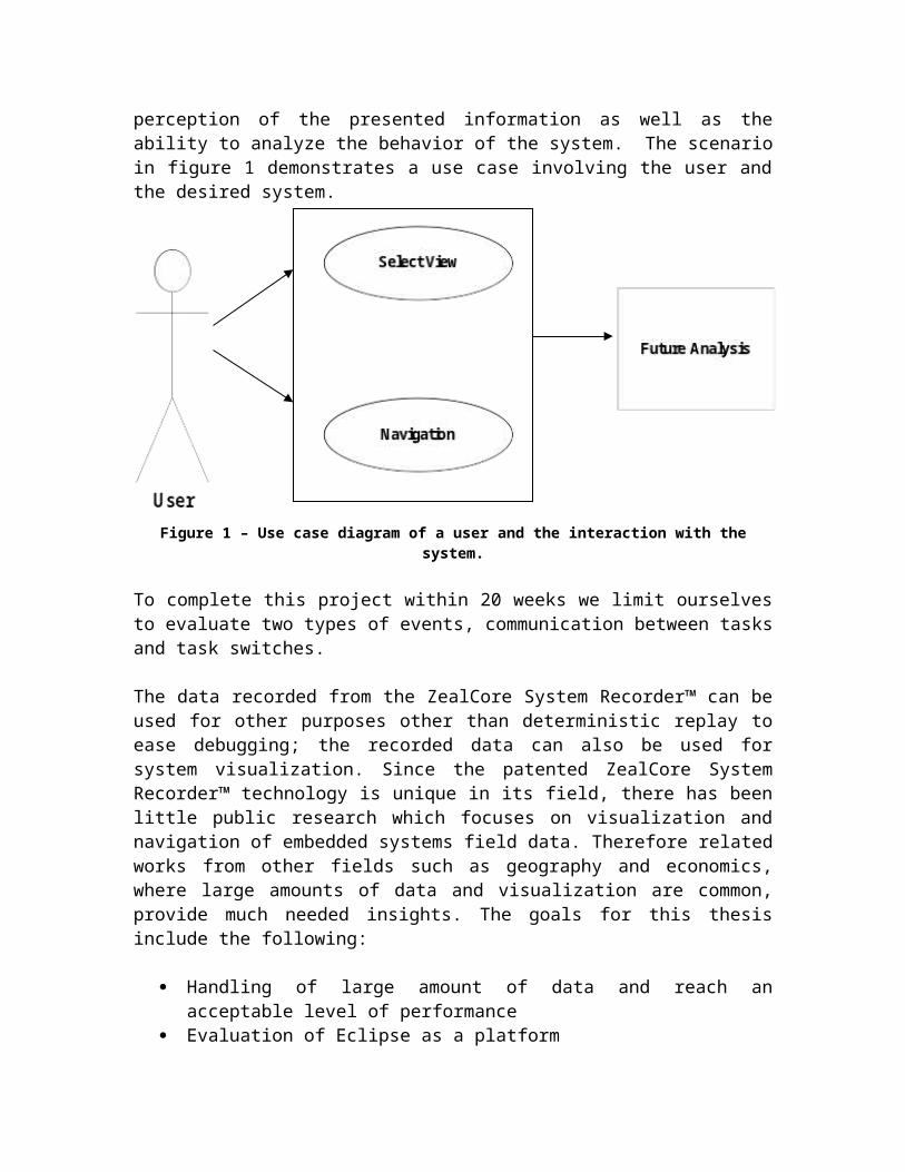
Figure 1 – Use case diagram of a user and the interaction with the system.

To complete this project within 20 weeks we limit ourselves to evaluate two types of events, communication between tasks and task switches.

The data recorded from the ZealCore System Recorder™ can be used for other purposes other than deterministic replay to ease debugging; the recorded data can also be used for system visualization. Since the patented ZealCore System Recorder™ technology is unique in its field, there has been little public research which focuses on visualization and navigation of embedded systems field data. Therefore related works from other fields such as geography and economics, where large amounts of data and visualization are common, provide much needed insights. The goals for this thesis include the following:

Handling of large amount of data and reach an acceptable level of performance Evaluation of Eclipse as a platform Developing a software tool which may be used on various platforms Navigation of a large amount of real-time data Visualization of real-time systems field data

Ultimately, these goals enable an approach to investigate how to efficiently manage large quantities of information, research visualization techniques as well as means to navigate within the vast amount data. Since ZealCore is interested in developing tools for the Eclipse platform a visualization prototype and navigation implementation is to be developed and deployed as an Eclipse plug-in. From the visualization prototype a user should be able to understand the system as a big picture.

Delimitations

The ZealCore System Recorder™ can record everything that is needed to reproduce the behaviour of a distributed real-time system; including but not limited to task switches, IPC-messages (Inter Process Communication) and messages between different systems nodes. The data generated is not comprehensible in itself and most types of events may require a separate visualization technique. To limit the scope to a reasonable level this thesis will only focus on visualization and navigation of system resources and task switches and IPC.

The rest of the thesis is divided into six major sections; the first section covers related work including distributed real-time systems, data storage methods and visualization techniques. The following problem analysis describes the main problem and breaks it down into tangible goals. The third section explains the model and method used to perform this thesis, the next section presents the proposed solution, after the solution section come the actual results analysis. The last section is a joint conclusions and future work, explaining the many items discovered during the thesis.

Related work Some of the relevant theory and related works relative to the main goals of this thesis are described in this section. As mentioned previously, the ultimate goals are to manage and visualize information gathered from a large amount of stored data. Before achieving these goals it is important to understand the concept of distributed real-time systems (DRTS) since they cover the scope of the field for this thesis work. In turn, DRTS may also contribute to large amount of stored data. With this a viable knowledge about some issues concerning DRTS monitoring including some hardware solutions and software solutions can be depicted. Furthermore, the theories about different models and architecture for large data storage will be discussed. Finally, to gain a perspective of how to develop a visualization large data set, some related works from different fields will be presented.

Distributed Real-Time SystemsReal-time systems which communicate across a network are referred to as distributed real-time systems. In computer technology it is often the goal to create reusable software, to reduce cost and shorten development time. However, while developing real-time systems it may not be possible to incorporate such reusable software. This is due to the level of uncertainties such as overhead, contributing to unpredictable behavior of the system. Such uncertainty may also lead to an unreliable system, which in turn could lead to severe consequences. This leads to the fundamental aspect of asynchronous and synchronous modeling. These models describe the deterministic behavior of DRTS. In an asynchronous model executions and message transmissions of a task have no predicted time intervals to assume the behavior of the system. Conversely, a synchronous model has predictable time intervals between its execution steps and message transmissions are received or sent with a fixed time interval [7]. In DRTS, it is prudent to enable the visualization of events to monitor the overall behavior of the DRTS. The act of monitoring a real-time system is invasive. The effect on the system(s) due to this is termed as the probe effect which means that unpredictable behavior of the system may occur during the monitoring process. There are several practices available which focuses on the development of DRTS monitors with a controlled level of probe effects or preferably no probe effects [8].

Monitoring Real-Time Systems

The ability to monitor distributed real time systems will enable visualization of the systems’ behavior, increasing the ability to debug and test the system. However, monitoring of distributed real-time systems in itself leads to failure if proper care is not taken. This includes factoring in the correctness of monitor’s logic and execution time. To monitor a system, is to interfere with the system which may lead probe effect where relative timing in the system is perturbed [8]. A monitoring tool that does not interrupt the system is ideal if configured for cost and performance efficiencies. Cost and

performance penalties could be incurred to affect the resources such as memory or I/O processing if when monitoring tools are removed or inserted prematurely on a target system [8]. The intrusion of monitoring real-time systems can be minimized and controlled to ensure that it does not affect the execution of critical tasks by applying solutions to handle timing errors. We will discuss some works including software and hardware approaches to handle timing error issues during the process of monitoring distributed real time system.

Dealing with Timing Errors

The most critical aspect of distributed real time systems is the predictability of task execution and without proper support from the kernel it is hard to derive the source of timing errors. A possible timing issue may occur during the testing of integrated modules. At the kernel level, a scheduler or a priority based dispatcher controls the cyclic execution which consists of one major scheduling cycle (the whole system) and subdivisions of minor scheduling cycles (a frame within the system) [16]. A frame (Fi) contains a set of routines which may be called from different peripherals. In a classical distributed real time system, a missed deadline for a frame is caused by routine integration and is undetected until the final integration of the frames. At this stage the task of determining which routine contributed to the failure becomes complex. Although each routine is tested and successful in meeting its timing requirements but after routine calls within each frame, the final integration testing fails due to a missed deadline for Fi.

Monitoring of distributed real-time systems may contribute to this timing error especially when unaccounted for within the system scheduler. The monitor may very well be a cause for a failure within the system. An approach to solve this problem, derived by Tokuda et al. is to develop an “integrated time-driven scheduler” [16]. The purpose of this scheduler is to explicitly consider the interference caused by monitoring process. By using the rate monotonic scheduling approach and including the time requirements for the monitor in the scheduler, we can treat the interference as a task. This task is to be scheduled along with the other set of hard periodic tasks, which leads to better prediction of systems’ activities.

Software Solution for Monitoring Distributed Real Time Systems

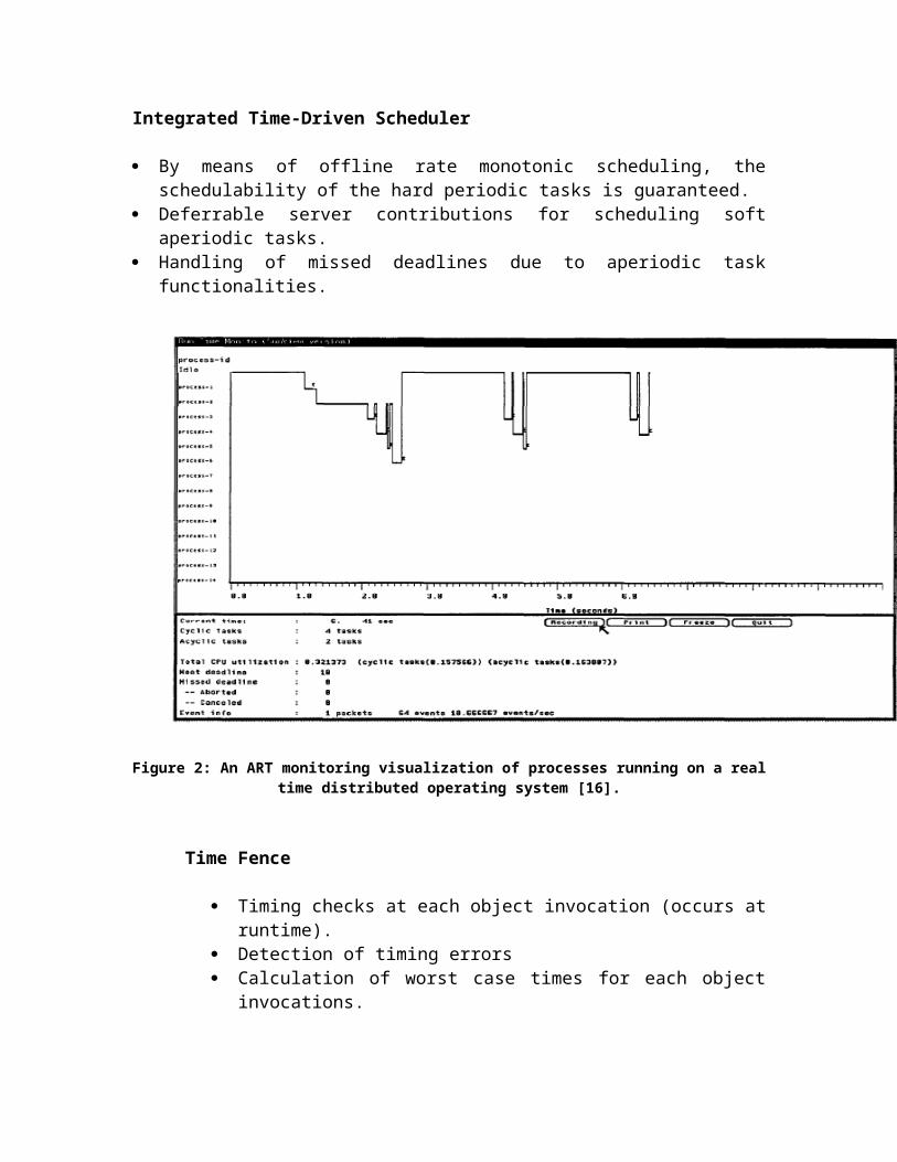
In the development of monitoring software, developers must consider that feasible hardware support is maintained to enable a global clock for all systems involved. A reporting process is responsible for relaying system events to the monitor, an offline schedule is performed and the process is treated as a periodic task with an execution time and deadline. The use of an object oriented model is useful when developing a distributed monitoring application. This approach enables the ‘primitives’ to simplify the navigation of the monitor’s visualization. As mentioned before, the ART developers incorporated an ‘integrated time-driven scheduler” in conjunction with the “time fence” approach. The contributions of these mechanisms are as following: [16]

Integrated Time-Driven Scheduler

By means of offline rate monotonic scheduling, the schedulability of the hard periodic tasks is guaranteed.

Deferrable server contributions for scheduling soft aperiodic tasks. Handling of missed deadlines due to aperiodic task functionalities.

Figure 2: An ART monitoring visualization of processes running on a real time distributed operating system [16].

Time Fence

Timing checks at each object invocation (occurs at runtime). Detection of timing errors Calculation of worst case times for each object invocations.

The design of the ART monitoring tool support the ability to handle timing exceptions by means of forward and backward recovery for a desired state. Figure 2 illustrates a snapshot of the monitoring visualization of ART. It is possible to see the running process on the y-axis and the time in seconds on the x-axis. With this tool it is also possible to see a record of on-time executions, missed deadlines, CPU utilization as well as other graphical components that enable a forward or backward recovery for the system.

Hardware Solutions for Monitoring Distributed Real Time Systems

As mentioned earlier, there are overhead issues to be considered in distributed real time systems such as memory management, I/O management and interrupt handlers. Unpredictability of processors for data streaming across communication protocols generates an unpredictable system. Most hardware capabilities include speed as an important feat for performance. However, speed is not considered as important as predictability when it comes to real time systems. The hardware solution to monitoring distributed real time systems is to optimize the kernel level services for better predictability.

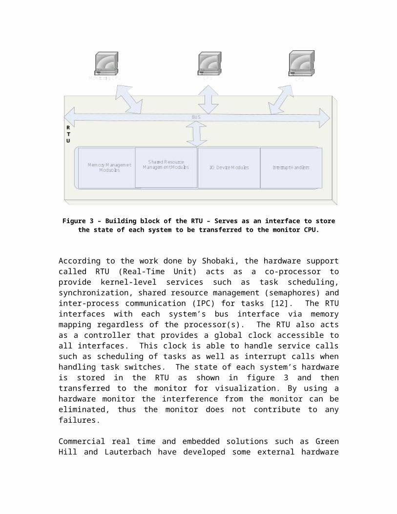
Figure 3 – Building block of the RTU – Serves as an interface to store the state of each system to be transferred to the monitor CPU.

According to the work done by Shobaki, the hardware support called RTU (Real-Time Unit) acts as a co-processor to provide kernel-level services such as task scheduling, synchronization, shared resource management (semaphores) and inter-process communication (IPC) for tasks [12]. The RTU interfaces with each system’s bus interface via memory mapping regardless of the processor(s). The RTU also acts as a controller that provides a global clock accessible to all interfaces. This clock is able to handle service calls such as scheduling of tasks as well as interrupt calls when handling task switches. The state of each system’s hardware is stored in the RTU as shown in figure 3 and then transferred to the monitor for visualization. By using a hardware monitor the interference from the monitor can be eliminated, thus the monitor does not contribute to any failures.

Commercial real time and embedded solutions such as Green Hill and Lauterbach have developed some external hardware which works in conjunction with targeted systems for hardware monitoring. The application of hardware monitoring has produced a non-intrusive solution towards the monitoring of distributed real time systems. Such hardware applications include e.g. SuperTrace Probe [10] by Green Hill and the PowerTrace [9] by Laubterbach Company. These hardware applications are solutions to achieving a non-intrusive mechanism of monitoring distributed real time systems. The fundamental behind these commercial hardware solutions is to eliminate timing errors caused by the probe effect. In other words, this special hardware is connected to the target system and has the ability to record events and instructions executed by the host processor. The hardware trace data are outputs to dedicated ports within the processor and consists of information about the execution of tasks. Although these hardware trace (monitoring) techniques solve the issues of probe effects, such hardware solution can indeed be very expensive when it comes to distribute real-time systems. Since each trace hardware is specific to a targeted system the system has to have sufficient amount of RAM allocated for hardware trace data. Furthermore, these hardware monitors are integrated via a network bus so that the monitoring systems are able to project collected data about the distributed real-time systems behavior.

Data Storage The computer storage and computer memory refer to the components, devices and recording media that is capable of retaining data for some interval of time. These devices provide one of the core functions of the modern computer of today. The former, computer storage, commonly refers to other types of recording media such as optical discs, magnetic storage such as hard drives and other types of storage devices which are slower but permanent and much cheaper compared to the primary storage. The latter, computer memory, usually refers to a solid state storage known as random access memory (RAM) and other forms of fast but temporary storage.

Due to the limitations in both these storage facilities, storage and processing of large amounts of data requires smart storage and processing techniques. A database together with a database management system is a well organized collection of data. For a given database there exist a structural description of types and facts stored within the database, this is generally known as a schema. The schema describes how data is represented in the database, and how records are related to each other. There are many numbers of different ways or techniques to organize such schemas. These techniques are usually known as database models or data models. The model that is most commonly used today is the relational model. The term database actually refers to the collection of related records, the software and tools used to manage and access these records are called the database management system (DBMS), however when the context is clear, most people use the word database to cover both meanings. [21].

Relational Database Management Systems

Relational databases are one of the most common ways of storing and retrieving data in any type of computer system. Relational databases are based upon the relational model which assumes that all data and associations between data can be represented as mathematical relations. The theory behind the relational model dates back to 1970 in which it was first proposed by E. F. Codd in a seminar paper [17]. The objectives of the relational model were specified as follows:

To allow a high degree of data independence, application programs must not be affected by modifications to the representation of the internal data. In particular by changes to file organizations, record orderings and access paths.

To provide a basis to deal with data semantics, consistency and redundancy problems. Codds’ paper introduces the concept of normalized relations which will be discussed later.

Commercial systems based on the relational model started to appear in the late 1970s. Nowadays, there are several hundred relational DBMS for most kinds of systems, ranging from mainframe to microcomputer environments. There are also several free open source database alternatives to commercial products. Free database such as PostgreSQL, Firebird DB and MySQL has gained in popularity over the years.

The relational model

Within a relational database management system the data is operated upon by some sort of relational language and these languages are based upon relational algebra and/or relational calculus. Relational algebra is a theoretical language with operations that work with one or more relations to define another relation without changing the original relation. Both the operands and the result is a relation which means that the output from one operation can be the input of another to enable the ability to nest expressions. The theory behind relational algebra, calculus and the usage of such languages is complex and not well suited for human interface, therefore other interface mechanisms exists. The de facto language for API interactions with RDBMS is nowadays the Structured Query Language (SQL). [18]

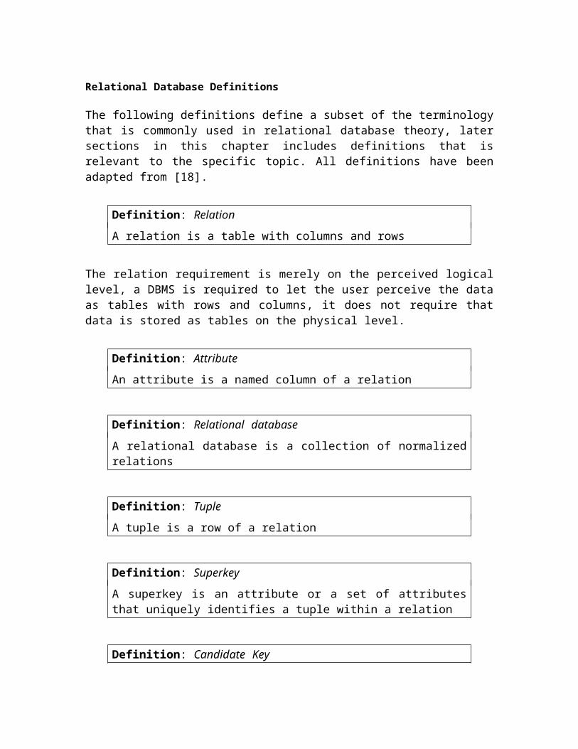
Relational Database Definitions

The following definitions define a subset of the terminology that is commonly used in relational database theory, later sections in this chapter includes definitions that is relevant to the specific topic. All definitions have been adapted from [18].

Definition: Relation

A relation is a table with columns and rows

The relation requirement is merely on the perceived logical level, a DBMS is required to let the user perceive the data as tables with rows and columns, it does not require that data is stored as tables on the physical level.

Definition: Attribute

An attribute is a named column of a relation

Definition: Relational database

A relational database is a collection of normalized relations

Definition: Tuple

A tuple is a row of a relation

Definition: Superkey

A superkey is an attribute or a set of attributes that uniquely identifies a tuple within a relation

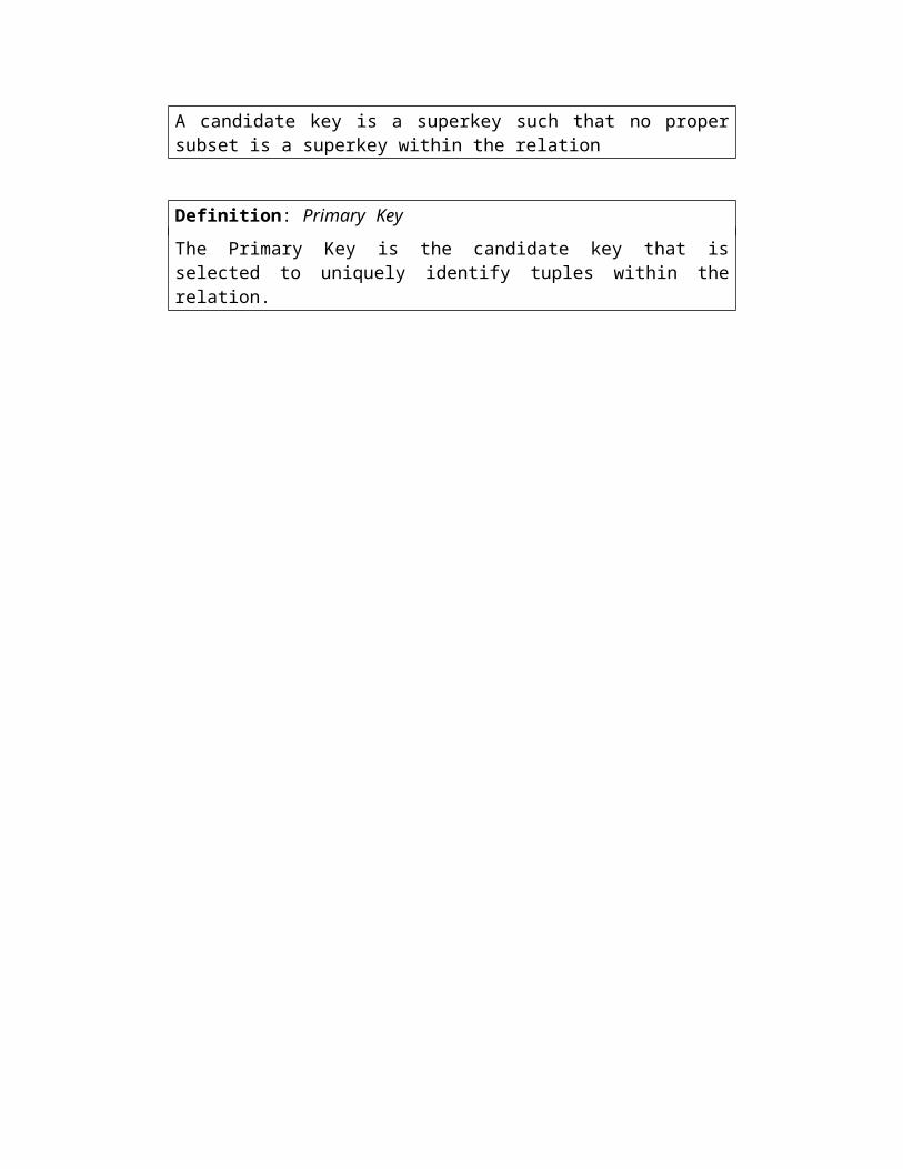
Definition: Candidate Key

A candidate key is a superkey such that no proper subset is a superkey within the relation

Definition: Primary Key

The Primary Key is the candidate key that is selected to uniquely identify tuples within the relation.

Normalized schemas

The main objective when designing a database for a relational system is to have a logical data model. The data model must be an accurate representation of actual data, the relationships and data constrains. To achieve this, a suitable set of relations must be identified. One technique to help design a well formed data model is called normalization. Normalization is often performed as a series of tests to determine if it satisfies or violates requirements for a given normal form. The benefit of complying to higher normal forms are that less redundant data is stored, changes to data may only need to be done at one row rather than two or more. If a change would require updating two or more rows and one or more rows are forgotten in the update, it would leave the database in an inconsistent state. The initial theory from 1972 defines only three normalization forms, elegantly named first, second and third normal forms. There are also more strong normal forms, such as BCNF (Boyce-Codd Normal Form), fourth and fifth normal form [20,18]. However most higher forms of normalization deal with very rare scenarios and for most types of system the 3NF is sufficient [18]. The following sections describe the first, second and third normalization forms.

Functional Dependencies

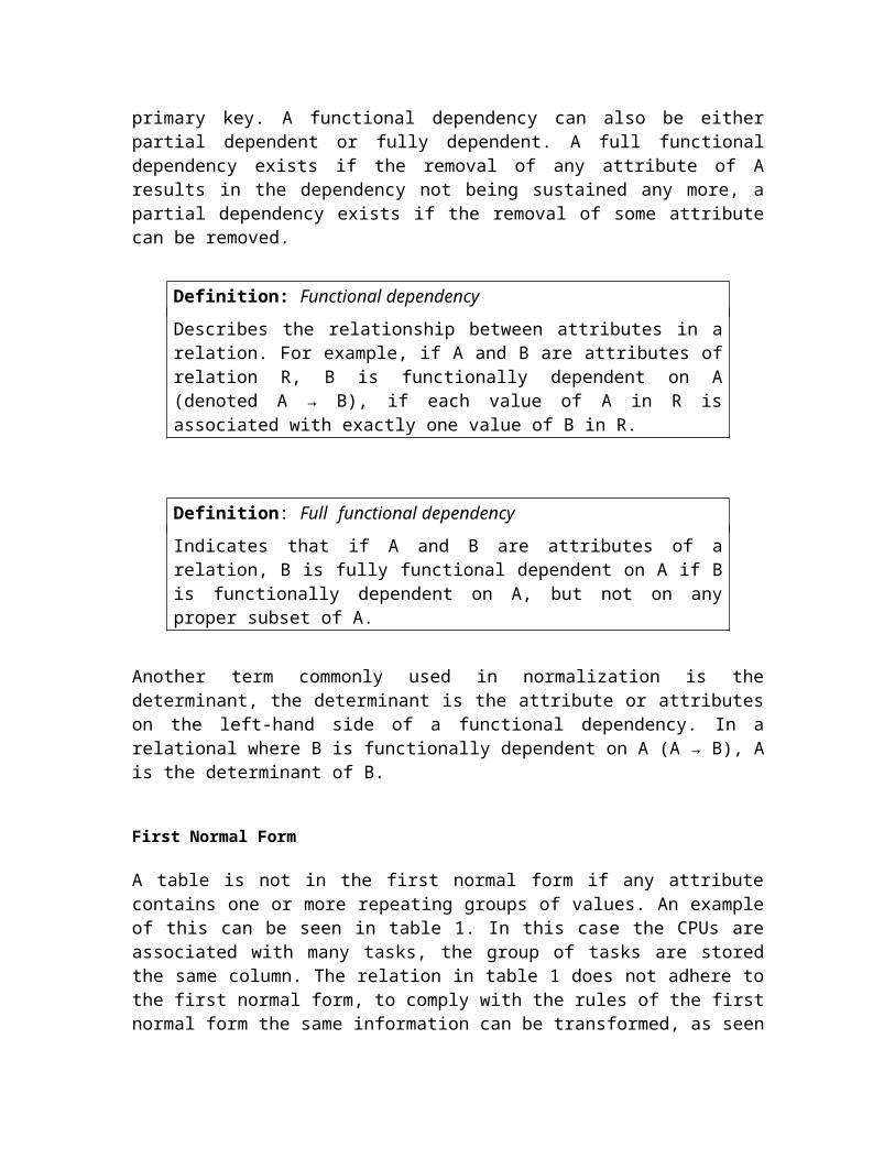
Functional dependency is a key concept in normalization. A functional dependency describes relationships between attributes within a table. If a functional dependency is present it is specified as a constraint between the attributes. As an example consider a relation R with attributes A and B where B is functionally dependent on A. If the value of A is known, there will be only one value of B in all rows within R, this also means that if two rows share the same value of A they will also have the same value of B. It should be noted that both A and B can be a set of attributes, for instance a relation can have a composite primary key. A functional dependency can also be either partial dependent or fully dependent. A full functional dependency exists if the removal of any attribute of A results in the dependency not being sustained any more, a partial dependency exists if the removal of some attribute can be removed.

Definition: Functional dependency

Describes the relationship between attributes in a relation. For example, if A and B are attributes of relation R, B is functionally dependent on A (denoted A → B), if each value of A in R is associated with exactly one value of B in R.

Definition: Full functional dependency

Indicates that if A and B are attributes of a relation, B is fully functional dependent on A if B is functionally dependent on A, but not on any proper subset of A.

Another term commonly used in normalization is the determinant, the determinant is the attribute or attributes on the left-hand side of a functional dependency. In a relational where B is functionally dependent on A (A → B), A is the determinant of B.

First Normal Form

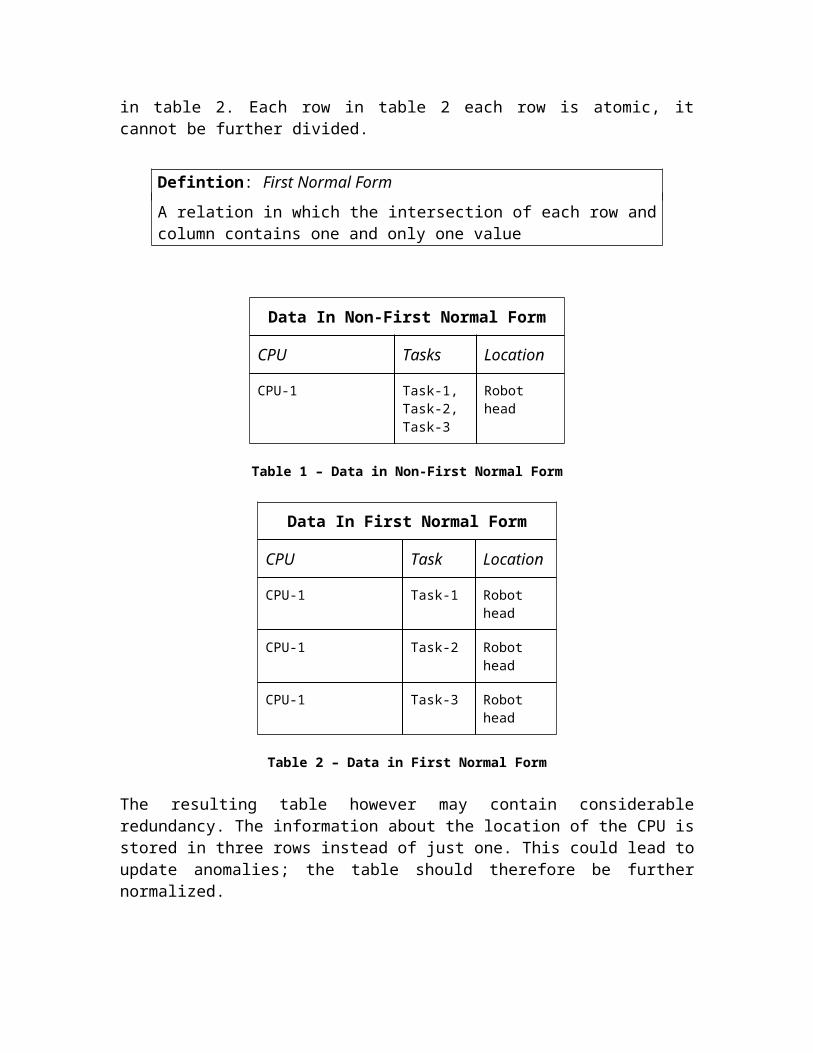
A table is not in the first normal form if any attribute contains one or more repeating groups of values. An example of this can be seen in table 1. In this case the CPUs are associated with many tasks, the group of tasks are stored the same column. The relation in table 1 does not adhere to the first normal form, to comply with the rules of the first normal form the same information can be transformed, as seen in table 2. Each row in table 2 each row is atomic, it cannot be further divided.

Defintion: First Normal Form

A relation in which the intersection of each row and column contains one and only one value

Data In Non-First Normal Form

CPU Tasks Location

CPU-1 Task-1, Task-2, Task-3

Robot head

Table 1 – Data in Non-First Normal Form

Data In First Normal Form

CPU Task Location

CPU-1 Task-1 Robot head

CPU-1 Task-2 Robot head

CPU-1 Task-3 Robot head

Table 2 – Data in First Normal Form

The resulting table however may contain considerable redundancy. The information about the location of the CPU is stored in three rows instead of just one. This could lead to update anomalies; the table should therefore be further normalized.

Second Normal Form

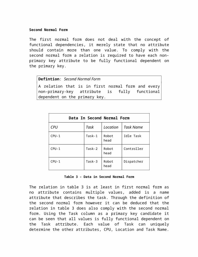
The first normal form does not deal with the concept of functional dependencies, it merely state that no attribute should contain more than one value. To comply with the second normal form a relation is required to have each non-primary key attribute to be fully functional dependent on the primary key.

Defintion: Second Normal Form

A relation that is in first normal form and every non-primary-key attribute is fully functional dependent on the primary key.

Data In Second Normal Form

CPU Task Location Task Name

CPU-1 Task-1 Robot head Idle Task

CPU-1 Task-2 Robot head Controller

CPU-1 Task-3 Robot head Dispatcher

Table 3 – Data in Second Normal Form

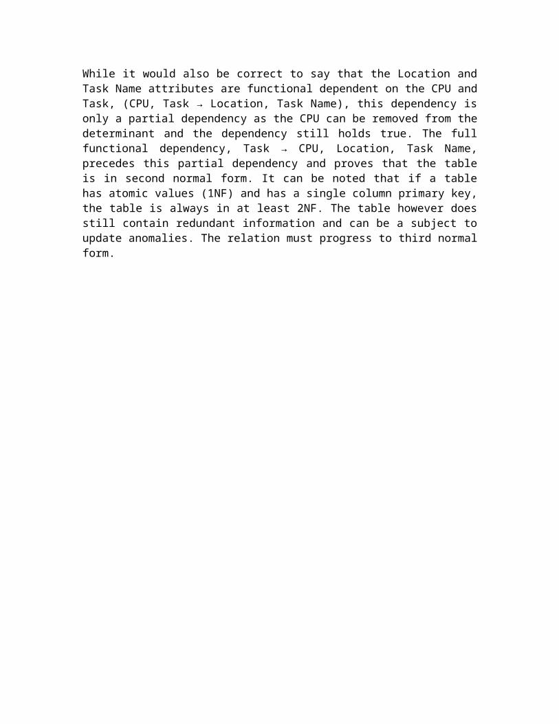
The relation in table 3 is at least in first normal form as no attribute contains multiple values, added is a name attribute that describes the task. Through the definition of the second normal form however it can be deduced that the relation in table 3 does also comply with the second normal form. Using the Task column as a primary key candidate it can be seen that all values is fully functional dependent on the Task attribute. Each value of Task can uniquely determine the other attributes, CPU, Location and Task Name. While it would also be correct to say that the Location and Task Name attributes are functional dependent on the CPU and Task, (CPU, Task → Location, Task Name), this dependency is only a partial dependency as the CPU can be removed from the determinant and the dependency still holds true. The full functional dependency, Task → CPU, Location, Task Name, precedes this partial dependency and proves that the table is in second normal form. It can be noted that if a table has atomic values (1NF) and has a single column primary key, the table is always in at least 2NF. The table however does still contain redundant information and can be a subject to update anomalies. The relation must progress to third normal form.

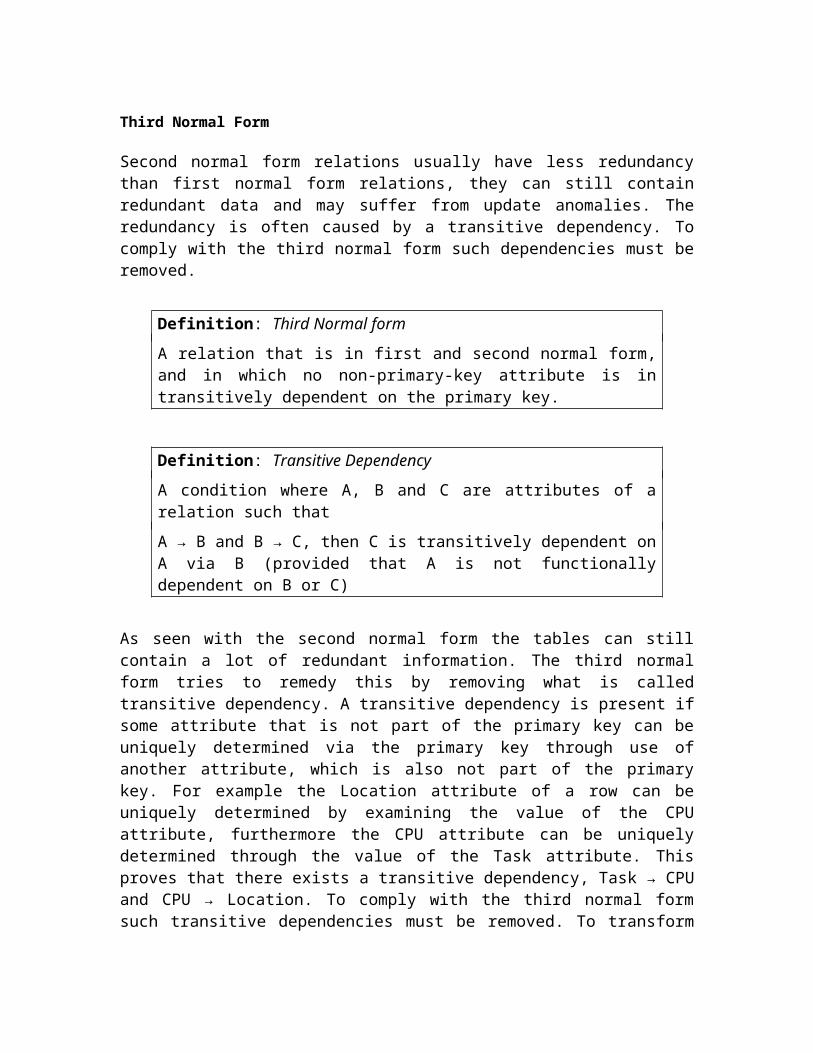
Third Normal Form

Second normal form relations usually have less redundancy than first normal form relations, they can still contain redundant data and may suffer from update anomalies. The redundancy is often caused by a transitive dependency. To comply with the third normal form such dependencies must be removed.

Definition: Third Normal form

A relation that is in first and second normal form, and in which no non-primary-key attribute is in transitively dependent on the primary key.

Definition: Transitive Dependency

A condition where A, B and C are attributes of a relation such that

A → B and B → C, then C is transitively dependent on A via B (provided that A is not functionally dependent on B or C)

As seen with the second normal form the tables can still contain a lot of redundant information. The third normal form tries to remedy this by removing what is called transitive dependency. A transitive dependency is present if some attribute that is not part of the primary key can be uniquely determined via the primary key through use of another attribute, which is also not part of the primary key. For example the Location attribute of a row can be uniquely determined by examining the value of the CPU attribute, furthermore the CPU attribute can be uniquely determined through the value of the Task attribute. This proves that there exists a transitive dependency, Task → CPU and CPU → Location. To comply with the third normal form such transitive dependencies must be removed. To transform the relation to third normal form the relation must be split into a new relation, along with a copy of the determinant.

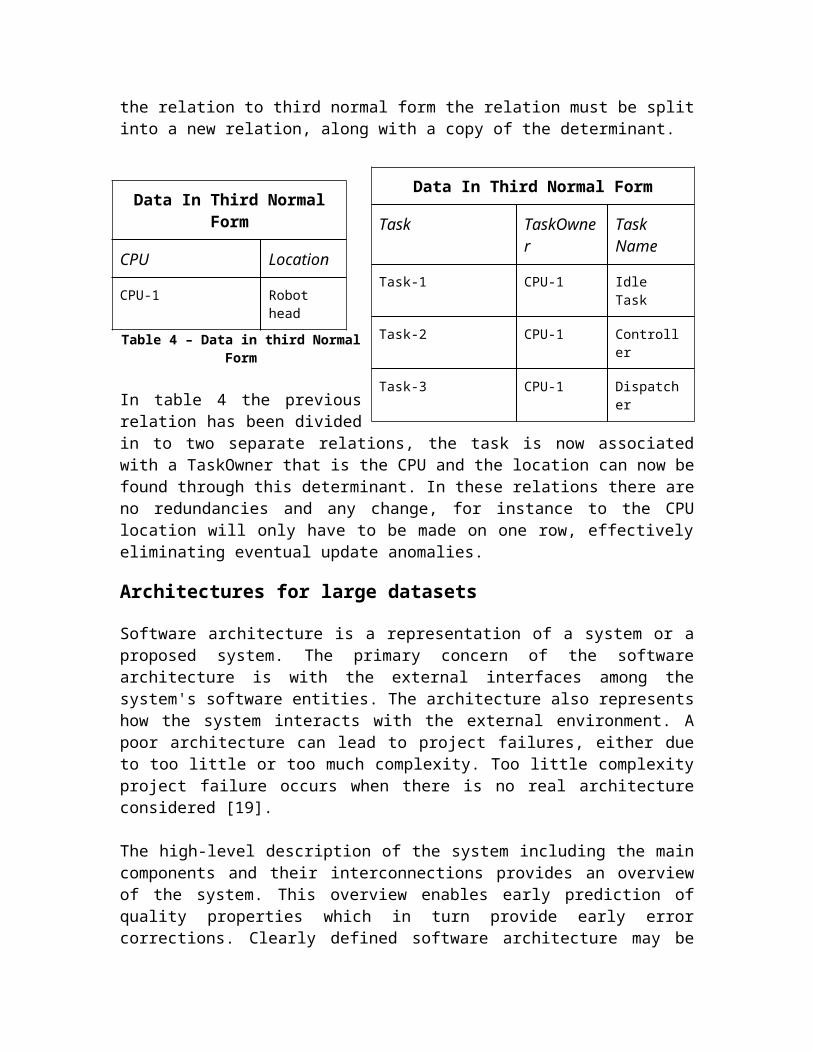
Table 4 – Data in third Normal Form

In table 4 the previous relation has been divided in to two separate relations, the task is now associated with a TaskOwner that is the CPU and the location can now be found through this determinant. In these relations there are no redundancies and any change, for instance to the CPU location will only have to be made on one row, effectively eliminating eventual update anomalies.

Data In Third Normal Form

Task TaskOwner Task Name

Task-1 CPU-1 Idle Task

Task-2 CPU-1 Controller

Task-3 CPU-1 Dispatcher

Data In Third Normal Form

CPU Location

CPU-1 Robot head

Architectures for large datasets

Software architecture is a representation of a system or a proposed system. The primary concern of the software architecture is with the external interfaces among the system's software entities. The architecture also represents how the system interacts with the external environment. A poor architecture can lead to project failures, either due to too little or too much complexity. Too little complexity project failure occurs when there is no real architecture considered [19].

The high-level description of the system including the main components and their interconnections provides an overview of the system. This overview enables early prediction of quality properties which in turn provide early error corrections. Clearly defined software architecture may be used to evaluate requirements and quality attributes such as:

Environmental issues - Where the equipment can be located; whether or not the software can operate at only one or several locations; if there are any environmental restrictions, such as magnetic interference that need to be considered.

Interfaces - Considerations to be made about the input, if it is coming from one or several system and if the output is going to one or several other systems. If there is a special way in which data must be formatted and if there is a special medium that the data must use.

Run-time behaviour - To determine whether or not there are any performance requirements and also includes the reliability, availability and the temporal behaviour.

Other development properties can also be estimated from an architectural view, properties such as cost, time, resources and work distribution. Over the years several proven architectural styles have emerged. An architectural style is a pattern of components with a given well known name. The benefit of having a common name for an architectural style is clear when discussing or examining a system. To say that a system is built in a layered architecture will instantly give others an understanding of the systems. Such knowledge will help when detailed implementation decisions must be made and what rules designers and programmers must adhere to. There are multiple architectural designs available, to gain as much as possible from the chosen architecture the designer must analyze the software requirements and chose the best-fit.

There is no architecture that is always the best choice; however the following sections describe two common and proven architectural styles commonly used for data access, the layered architecture which is often used at the application level and the client-server architecture which allows clients to connect to powerful data storage servers.

Layered Architecture

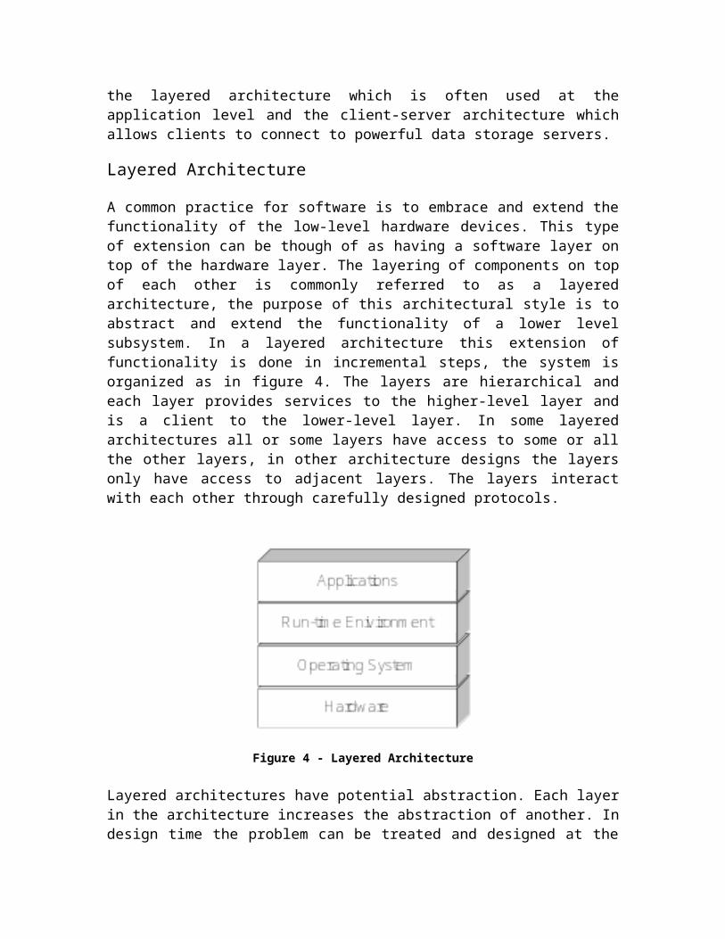
A common practice for software is to embrace and extend the functionality of the low-level hardware devices. This type of extension can be though of as having a software layer on top of the hardware layer. The layering of components on top of each other is commonly referred to as a layered architecture, the purpose of this architectural style is to abstract and extend the functionality of a lower level subsystem. In a layered architecture this extension of functionality is done in incremental steps, the system is organized as in figure 4. The layers are hierarchical and each layer provides services to the higher-level layer and is a client to the lower-level layer. In some layered architectures all or some layers have access to some or all the other layers, in other architecture designs the layers only have access to adjacent layers. The layers interact with each other through carefully designed protocols.

Figure 4 - Layered Architecture

Layered architectures have potential abstraction. Each layer in the architecture increases the abstraction of another. In design time the problem can be treated and designed at the highest abstraction, the solution can then be further decomposed into lower-level layers. The layered architecture also makes it relatively painless to change the implementation of a layer; such changes will in the worst case only affect the adjacent layers, or all the layers that communicate with the changed layer. For the same reason, a layer can easily be reused with modifications to only adjacent layers.

It may not always be easy to architect a system into layers, the abstraction levels may not easily distinguished when examining the requirements. When creating a layered design there may be a performance penalty from the extra coordination between layers.

Façade Design Pattern

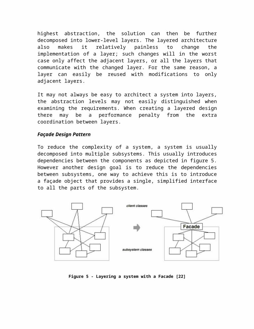
To reduce the complexity of a system, a system is usually decomposed into multiple subsystems. This usually introduces dependencies between the components as depicted in figure 5. However another design goal is to reduce the dependencies between subsystems,

one way to achieve this is to introduce a façade object that provides a single, simplified interface to all the parts of the subsystem.

Figure 5 - Layering a system with a Facade [22]

The façade design pattern can also help out when you want to create a layered architecture, a façade object can be used to define a single entry point to each layer in the system. If the subsystems are dependent, these dependencies can be simplified by introducing a façade object between the systems. The introduction of façade objects makes the subsystems communicate solely through their facades.

Client Server Architecture

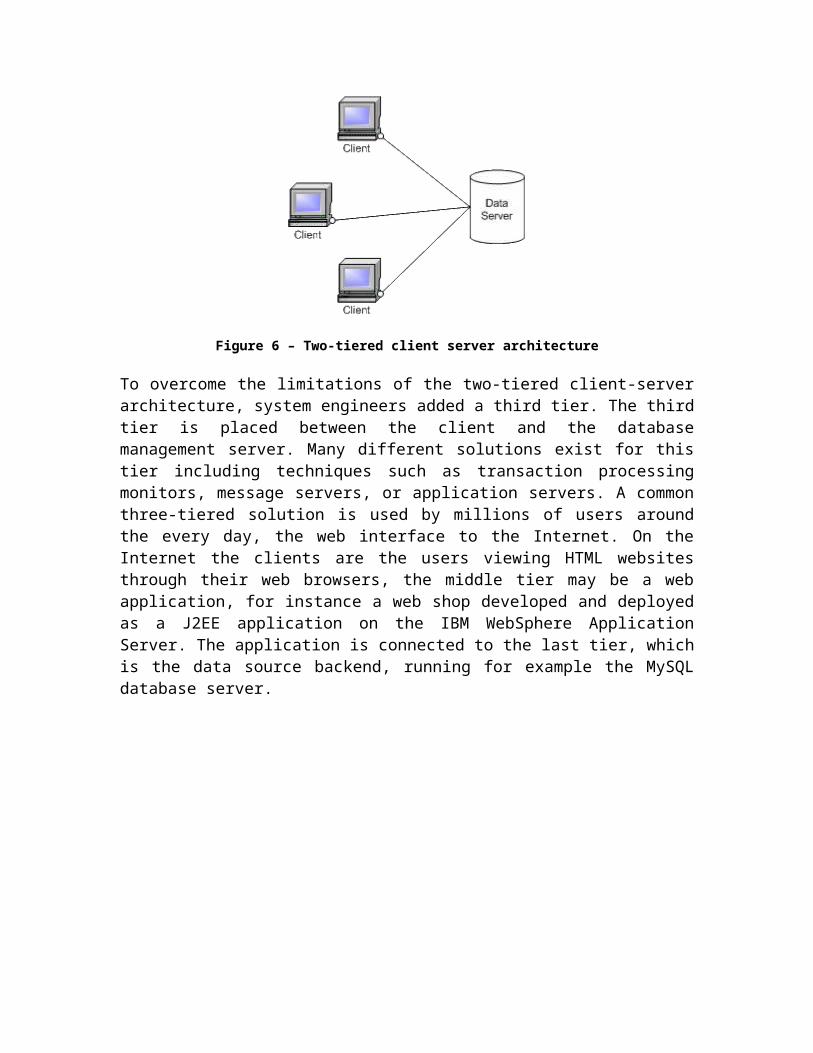
A common architectural style for interacting with data sources is the client-server architecture. The client-server architecture is composed of a service provider called a server, and one or more clients requesting this service. A single machine may be both the server and the client, however it is usually the case that one or more powerful computers act as the server and the clients can issue requests for services over a network. The server can return a reply specific to the request rather than a whole file as is the case in file-sharing architectures. As this message-based approach become very versatile and modular, the architecture can shrink and grow to handle changes in performance requirements. It may be cheaper to add a new server node or upgrade the existing server than to upgrade the capacity of all the clients. This means that the structure of client-server architecture has improved flexibility, interoperability and scalability compared to centralized systems. In classic two-tier architecture the user interface resides on the clients, and the database application resides on the server hardware, serving many clients. The two-tier solution seems to be a good solution for workgroups, depending on the business logic, up to about a 100 people interacting on a local area network. The limitation is the result of the server maintaining connections through keep-alive messages to each and every client even though there are no service requests

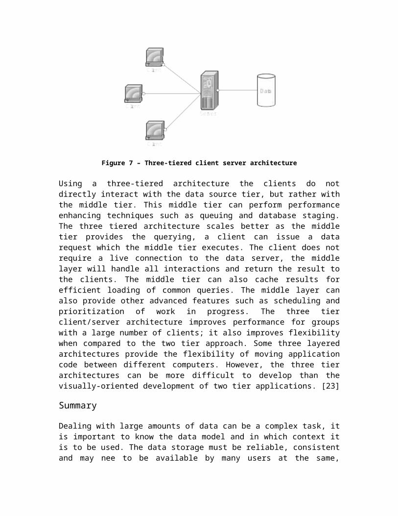
Figure 6 – Two-tiered client server architecture

To overcome the limitations of the two-tiered client-server architecture, system engineers added a third tier. The third tier is placed between the client and the database management server. Many different solutions exist for this tier including techniques such as transaction processing monitors, message servers, or application servers. A common three-tiered solution is used by millions of users around the every day, the web interface to the Internet. On the Internet the clients are the users viewing HTML websites through their web browsers, the middle tier may be a web application, for instance a web shop developed and deployed as a J2EE application on the IBM WebSphere Application Server. The application is connected to the last tier, which is the data source backend, running for example the MySQL database server.

Figure 7 – Three-tiered client server architecture

Using a three-tiered architecture the clients do not directly interact with the data source tier, but rather with the middle tier. This middle tier can perform performance enhancing techniques such as queuing and database staging. The three tiered architecture scales better as the middle tier provides the querying, a client can issue a data request which the middle tier executes. The client does not require a live connection to the data server, the middle layer will handle all interactions and return the result to the clients. The middle

tier can also cache results for efficient loading of common queries. The middle layer can also provide other advanced features such as scheduling and prioritization of work in progress. The three tier client/server architecture improves performance for groups with a large number of clients; it also improves flexibility when compared to the two tier approach. Some three layered architectures provide the flexibility of moving application code between different computers. However, the three tier architectures can be more difficult to develop than the visually-oriented development of two tier applications. [23]

Summary

Dealing with large amounts of data can be a complex task, it is important to know the data model and in which context it is to be used. The data storage must be reliable, consistent and may nee to be available by many users at the same, dealing with concurrency problems. The RDBMS provide a standardized way known by many developers and there are many vendors of free and commercial systems. By separating the data from the application using a database server the system can automatically achieve a client-server architecture. The client-server architecture also makes it possible for the underlying database implementation to change transparent to the clients. Remember that one of the goals with the relational database model was to have a high degree of data independence; the clients must not be affected by modifications to the data representation. If the client application is built with a layered architecture, the client-server architecture provides means to change the database implementation completely. The new implementation does not even have to be a relational database. Other data storage technologies such as object-databases or something completely different can be used.

VisualizationA graphical presentation is commonly used to gain a better perception of raw data. This can be an invaluable tool as a database may contain a very large set of data. A viewer can gain knowledge about the characteristics of the information stored in the data storage as well as the ability to navigate the data. The type of information stored in a database may include multidimensional data, processes or event records. As the amount of data increase, the complexity of the data structure becomes more difficult to manage. Therefore effective means of exploring information has been developed to establish a better perception of such data complexity. There are various types of visualization techniques available to project desired concepts effectively. Techniques such as graphs, charts, plots or maps may be used for specific fields and their applications. A combination of these techniques may also be used to produce a feasible perception of a given application. For instance, graphs are efficient when an application involves structures and functional relationships between entities. Such applications could enable an analytical deduction of valuable information. Graphical views may be represented in 2D or 3D along with animated styles, or as static views of the presented data. Data animation usually demonstrates significant changes of measurements over time [2]. Data visualizations are commonly controlled by components such as buttons, icons and text fields. Although these components are not necessary, manual inputs to control the views may become tedious for the user as well as time consuming.

Dynamic and Static Views

Dynamic and static views are techniques used in the visualization process. The difference between these two techniques is that a dynamic view incorporates animation to view, dynamically, the changes in a data’s characteristics over time. On the other hand, a static view illustrates the data at a point in time, or a fixed time series. Although, using a static view would be effective when seeking to make an analysis for a data at a particular time, the ability to make further detailed analysis about the data’s overall characteristics can become limited without animation.

The basic concept of an animated view is the ability of a display to update its content at a sufficient rate. Such animations would resemble watching a smooth and continuous motion of the represented data. An example application that utilizes animation is weather forecasts; the screen is updated periodically to show variations in weather over several locations across time.

The disadvantage of using a static view when analyzing the weather forecast is that we cannot get a better prediction about the type of weather occurring or will occur in the near future. The proceeding sections of this chapter will discuss some related work which involves the visualization of geographical data and economical data as well as their navigation techniques. Prior to the discussion pertaining to these types of visualizations, we will focus on some tradeoffs of using 2-D or 3-D visualization techniques.

2-D and 3-D Visualization Techniques

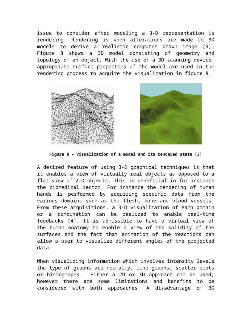
Dimensions are used to express the characteristics of objects within a spatial region. Dimensions may used to describe an object’s characteristics with respect to time, quantity or any other parameter. Such concepts contributes to the use of 2-D and 3-D graphing techniques. These techniques are used in data visualization and are crucial in the communication and analysis of data [2]. 2-D graphs are commonly enumerated by using X-Y coordinates while 3-D requires X, Y and Z coordinates. A situation that would use the 2-D representation is when the speed of a moving car is recorded relative to time. On the other hand, a 3-D representation would be more valid for aircrafts since we have to include altitude in the measurements. Another core issue to consider after modeling a 3-D representation is rendering. Rendering is when alterations are made to 3D models to derive a realistic computer drawn image [3]. Figure 8 shows a 3D model consisting of geometry and topology of an object. With the use of a 3D scanning device, appropriate surface properties of the model are used in the rendering process to acquire the visualization in figure 8.

Figure 8 – Visualization of a model and its rendered state [3]

A desired feature of using 3-D graphical techniques is that it enables a view of virtually real objects as opposed to a flat view of 2-D objects. This is beneficial in for instance the biomedical sector. For instance the rendering of human hands is performed by acquiring specific data from the various domains such as the flesh, bone and blood vessels. From these acquisitions, a 3-D visualization of each domain or a combination can be realized to enable real-time feedbacks [4]. It is admissible to have a virtual view of the human anatomy to enable a view of the solidity of the surfaces and the fact that animation of the reactions can allow a user to visualize different angles of the projected data.

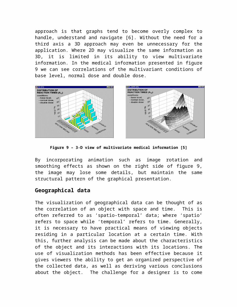
When visualizing information which involves intensity levels the type of graphs are normally, line graphs, scatter plots or histographs. Either a 2D or 3D approach can be used; however there are some limitations and benefits to be considered with both approaches. A disadvantage of 3D approach is that graphs tend to become overly complex to handle, understand and navigate [6]. Without the need for a third axis a 3D approach may even be unnecessary for the application. Where 2D may visualize the same information as 3D, it is limited in its ability to view multivariate information. In the

medical information presented in figure 9 we can see correlations of the multivariant conditions of base level, normal dose and double dose.

Figure 9 – 3-D view of multivariate medical information [5]

By incorporating animation such as image rotation and smoothing effects as shown on the right side of figure 9, the image may lose some details, but maintain the same structural pattern of the graphical presentation.

Geographical data

The visualization of geographical data can be thought of as the correlation of an object with space and time. This is often referred to as ‘spatio-temporal’ data; where ‘spatio’ refers to space while ‘temporal’ refers to time. Generally, it is necessary to have practical means of viewing objects residing in a particular location at a certain time. With this, further analysis can be made about the characteristics of the object and its interactions with its locations. The use of visualization methods has been effective because it gives viewers the ability to get an organized perspective of the collected data, as well as deriving various conclusions about the object. The challenge for a designer is to come up with the best possible means of designing a feasible visualization tool for geographical data. There are various works performed for the visualization of spatio-temporal data. The two that will be discussed in this section are works by Andrienko et al.’s task driven visualization software and Biswas’ TEMPVIS visualization tool.

According to the work done by Andrienko et al., they developed three different tools that were each developed to view a certain type of spatio-temporal data. The purpose of deriving these tools was to be able to perform analysis of data characteristics upon dynamic interactions across time. As mentioned previously, spatio-temporal data are data consisting of time, space and objects. The purpose of their work was to describe visualization techniques of three different types of data; including instant events (static), object movement (animated) and changing thematic data (animated). An application of these data types was used to develop a visualization tool for the ‘Naturdetekitve’ project. Users of this tool are able to view geographical information about nature including animals, plants and natural disasters.

The development of ‘TEMPVIZ’ was done to create a tool that enables the “use of animation with liked graphics for the visual explanation of spatio-temporal data” [11]. The motive for this development is that it is important to be able to identify vegetation changes over time with various occurrences of land use. To get a better understanding and analysis of the represented data, the use of animation was incorporated in the views.

Geographical Views

Maps are commonly used as the preferred graphical tools for the visualization of geographical data. Since geographic data tends to be quite large as well as distributed, the use of maps can communicate such spatial information to the views.

Figure 10 below demonstrates observations derived from ‘Naturdetektive’ project [15]. The geographic data is represented by means of a map to enable a comprehensible view of the geographic locations that were being observed.

Figure 10 - Geographic visualisation of events which occurred in nature. This data was collected for

the ‘Naturdetektive’ project [15].

The dynamic visualization of events over time is controlled by a time manager as shown on the bottom right side of figure 10. Included in the view are icons of the various objects that have been recorded such as plants, animals and earthquakes.

Navigation of Geographical Data

The TEMPVIZ project contributes several components to allow a user to navigate through the recorded data. Some graphical components that are used to aid in such navigation are:

Time manager, a component to adjust time Time marker, a component that moves horizontally to desired time mark. A user is able to click on an icon to represent the type of species to view.

The navigation of TEMPVIS as described above is made possible by the graphical controls added to the views. In each view, there are buttons, colored images (legends) and toggle buttons which carries out specific actions. It is possible to navigate static views as well as animated views. For example, a static view, can be zoomed in or out for a more detailed analysis of a particular area on a map. This enables the user to:

Select an area of interest Click on the zoom in or zoom out button Clicking on a colored point on the selected area, the pixel information can be

displayed. Pixel information may include properties such as the characteristics of that area in terms of the concentration of chlorophyll, time and location (TEMPVIS).

For the navigation of dynamic views, the use of a play button and graph move buttons enables an animation of the state changes. A user also has the option of stopping the animation or performing a reverse play back of desired state views [11].

Economic Data

To deduce viable information from economical data, a feasible visualization method is necessary. Since economic data is generated from financial information, it is possible to classify these data as an underlying subset. Another concept is that “economic data is also important for the business world to judge the general situation of an economy” [14]. The low level view of an economic data structure can be modeled as a calculated value as output from formulas performed implicitly that generates this value. Lux uses an iceberg metaphor to explain this structure.

Figure 11 - The apex contains the economic value. The second level holds the variables used to derive the formula that generates the value [14].

The formulas are entities within data storage so that queries to them would produce the desired result to be viewed. Since economic data tends to be large and complex, an effective means of visualization technique would enable a viewer’s ability to have a better understanding of the data. Examples of economic applications are ones to analyze and view gross national products (GNP), stock market reports, exchange rates and tax revenues.

The following section will discuss the works done by Keim and Lux et al. in regards to the techniques they used to view large sets of economic information. Keim et al. describes a recursive pattern technique used in the visualization of stock market and exchange rates applications. Lux describes two approaches to visualize GNP information for countries. The first approach is based on geographic views while the other approach focuses on global economic development.

Economic Views

The recursive pattern can be used to explore stock market information. It consists of two different databases with stock prices and exchange rates respectively. The concept of the recursive patter technique is to view data that is arranged from left to right and then right to left. The recursive pattern is beneficial for the stock market because more data items can be viewed at once, over a long period of time. Since stock market data tends to be quite large, the view used for the recursive pattern is pixel oriented where each data item is represented by a pixel. The arrangement of data is based on an algorithm that involves the width (# of columns), height (# of rows) and the recursive level i. This visualization is used to evaluate stock market prices based on various views. An explorer view contains four different levels. The first level show the exploratory pattern for days, level 2 represented the week, level 3 represented the months and level 4 represented the years. Furthermore, another view shows statistical information such as similarities between stocks and their prices over a time period. A 2D x-y view of such a plot across time

Value

Formula,Time, Countries, Companies,

Relations & Dependencies

Any information Structures

would be a disadvantage since only about 500 data items could be viewed at a time [13]. However, by using the pixel oriented-recursive pattern, a view of intensity of stock events is possible, where darker colors represent higher intensity.

Figure 12 – 3-D view of GNP for countries to deduce information about export and import between countries [14].

Lux describes various graphical techniques to visualize GNP for countries. The important elements that are necessary in the views are the country, the timestamp and a formula. Once these are visible, a user is able to generate dynamic representations based on their selections. The possible categories of GNP for a selection are import, export and exchange rate information. The following graphical components were used in the visualization technique:

2D or 3D Maps (Globe) - To view different regions as they evolved or declined economically and to deduce the level of changes or improvements required.

Bar Graphs - To show relationship between two entities.

2D Arrows - To view interaction between two countries.

Navigation of Economical Data Views

When navigating through economic data, a viewer is able to utilize the graphic tools on the view in an efficient manner to generate the desired result. Of course it is also conventional to incorporate animation to perform better analysis of the views. In reference to Lux’s GNP example, a user can generate an animation of the different views based on their selections and inputs. As an example, if a user wants to analyze a view of imports around the globe, then the user would first select ‘import’ from the list of categories, the screen then displays a global map with the 2D arrows pointing from one importing country towards the export country. The screen is then updated for the user’s view. In reference to Keim et al., navigation of the stock market view is made possible by incorporating the following into the visualization.

Time - Time related ordering of data items where pixels are presented from left to right as time increases.

User defined parameters - To specify the attributes required in the view. For example, with the use of

Color - The HSI (hue/saturation/intensity) color model is used to map high data value to light color and low data values to dark colors.

Summary

In this section we have learned that there are numerous fields for which visualization techniques are used to graphically present data and their underlying characteristics. Based on the different practices considered, we can generalize that the use of dynamic visualization is preferred to static visualization when detailed analysis about a data is required over a period of time. The two types of data discussed is geographical data and economic data. The strategies used in the visualization of these two types of data incorporate some aspects of the dynamic and static styles depending on the situation. We refer to geographical data as spatio-temporal in that we are dealing with objects in conjunction location and time. On the other hand, economic data are financial information generated within the business world. Although these two types of data differ semantically, they both exhibit similar concept when it comes to visualization techniques. The use of maps is incorporated as a tool for the visualization of both geographical and economical data. In the case of the ‘Naturdetektive’ and the TEMPVIS visualization tool, it is possible to deduce spatial information and vegetation changes respectively. The manipulation of such large data is controlled by means of proper navigation. Hence, we are able to view an animated presentation of these data with the help of time control components. Also incorporated in the geographic view is the ability to filter information, as demonstrated in the ‘Naturdetektive’ visualization. A user is able to select what kind of data they would like to view on the map. By using the filtrating method, it is possible

to reduce the level of cluster on the display, including the elimination of unnecessary information. As for the visualization of economic data, the use of map is used purposely to view global economical development. However, the process of filtering is incorporated in the visualization to have only information of the specified type of transaction (import or export) on the display. The concept of filtrating is applied in the recursive pattern method. This is achieved by incorporating levels of exploration, whereby a user can make a selection for a desired view.

Along with the filtering technique, it is imperative to consider whether to use 2-D or 3-D graphing technique for the visualization. As mentioned earlier there are some limitations and benefits of using one graphing technique over the other. As 2-D graphs presents a flat view data, 3-D graphs present a data objects in a virtually real manner. A limitation of using 2-D graphs over 3-D is based on the fact less information is presented. However, the use of 3-D graphical representation creates a higher level of complexity which could be problematic for most applications.

The application of these findings in these sections aid and supports the method of developing the visualization prototype. The use of filtering during exploration of data can help reduce the level of complexity for visualization views. Also, the use of a 2-D graph is preferred since the prototype will only be demonstrating messages and controlflow changes between tasks across time.

Problem Analysis

The thesis consists of several tasks, all of which should be solved in a consistent manner to be able to provide a coherent product. First the possibly vast amount of data generated by the ZealCore System Recorder™ need an efficient and manageable storage facility. This also includes finding architecture and methods that give acceptable performance in terms of user perceived delays when accessing information. The stored data is used as a basis for visual system analysis. The visualization should let the user observe the information at different levels of abstraction. At the highest level, the user should be able to get “the big picture”; while at the lower levels the views provide more detailed information.

Due to duration of this project, we are limited to evaluating two types of events which are namely inter-process communication of tasks and task switches. Overall the following is to be depicted based on our initial goal:

Handling of large amount of data and reach an acceptable level of performance – Since we will be using the Eclipse plug-in for our visualization, it is important to determine which method is feasible to handle both back end and front end features. In the case of back end, we are referring to the database which will be used to store our data. Data persistence is important here because we need a database (preferably freeware) and a query language. Since the issue of performance is essential, we will need to consider different methods of inserting and retrieving data at a considerable rate. Finally, the front end application which involves how the views should be structured for best performance.

Evaluation of Eclipse as a platform – We should study how we can develop an Eclipse plug- in by becoming familiar with the eclipse platform. Along with this, we should determine the possible types of views which are necessary within the plug in for a user to get the big picture of the stored data.

Developing a software tool which may be used on various platforms – We should analyze different platforms such as Windows, UNIX or Solaris since we want our prototype to run on these platforms

Navigation of a large amount of real-time data – We will incorporate within our visualization tool, features that are not complex but easy to use by a user. Navigational strategies such as the ability to step forward and backward to replay task events will be added.

Visualization of Real-Time systems field data – To master this concept, various related works and practices within this field will be studied. The deduction to be made from the visualization is the behaviour of a system based on the events recorded and visualized in real time.

Model/methodSoftware Process ModelOur method of developing the visualization plug-in prototype is one illustrated in the figure 13 below. This model follows an iterative development paradigm where the project is broken down into various phases. Next, each phase goes through the waterfall process model. In other words, a mini waterfall process was used to model each phase of the process iteratively. Over the course of the project, we discovered that utilizing this method allowed us the ability to get verification of each phase with previous stages in the process before moving on to the next phase of the development. We felt that such model would aid in the delivery of the prototype within the time limit of this thesis.

Figure 13 – The software process model

Requirements and Specification

This has been explained in the background and problem formulation section. However, in the model, we have two categories of requirements and specification. Informal category refers to initial requirements that were specified by ZealCore. This is where we were given a general overview of the project, ZealCore System Recorder™ technology and a list of operations they would like to see incorporated in the visualization. Over the duration of the project, a formal category surfaced as the specification changed slightly to improve the software development. The requirements for our prototype include to the following.

Concept of Eclipse Plug-in

Figure 14 illustrates the overall architecture of Eclipse platform. Generally, the concept of a plug-in is that it is an extension of a system’s functionality. The Eclipse platform is considered a “Rich Client” platform and this is due to the fact that it is ideal for building applications that require access to backend resources such as databases [1]. We can also refer to the Eclipse platform as an integration point since tools that were built on eclipse platform can be integrated with other tools and applications that were also built on the Eclipse platform. Such integration may occur regardless of which programming language was used in the tool or application’s development.

In the development of the prototype visualization plug-in will be developed to extend the functionalities of each of the subsystems within the Eclipse architecture.

Figure 14 - The Eclipse platform architecture. [1]

The Eclipse Platform workbench consists of API which contributes to the development of the UI presented to a user [1]. To aid in the development are two toolkits called SWT (Standard Widget Toolkit) and JFace. SWT is OS independent and provides an API which enables the implementation of widgets e.g. lists trees and buttons that are common to the native operating system. The JFace toolkit differs from SWT by acting as a wrapper for SWT. JFace is OS independent and consists of classes which transparently work with SWT widget [1]. The two domain features of JFace are actions and viewers. JFace actions are user commands which can be activated by interacting with widgets e.g. clicking a button or selecting a menu item. On the other hand, viewers contain a collection of SWT widgets including a “higher-level semantics available for SWT widgets” [1].

Firebird RDBMS

Due to the limited time we have to complete this thesis work, ZealCore has suggested that we run a simulation of our visualization prototype from data stored within a freeware Firebird database as opposed to the live data from the ZealCore System Recorder(TM). Firebird is an open source relational database management system that is useful for the storage of very large data sets. It was developed to use many ANSI SQL features to run on several platforms including Windows and several Unix platforms. When data is processed we are able to populate the database with our generated data. Conversely, at the view part, various queries are made to retrieve the data while the views project the desired visualization.

Generation of simulated embedded systems data

A feasible approach is to be made to generate the desired embedded systems data by taking into account the specified benchmarks as shown in figure 15. Considerations have to be made about the best way of optimizing the performance while inserting and retrieving data from the database. Another consideration is to come up with a manageable structure for all the objects derived in the generator.

Figure 15 – Specification for the generation of embedded systems data

Graphical Visualization of data

With the aid of Eclipse SWT and JFace graphical tools, we were able to come up with various views for our prototype. With this the navigation of the prototype is to aid and user to study and deduce viable information about the execution of tasks in a distributed system.

Domain Identifications and Attributes

Based on the requirements and specifications we were able to derive the necessary domain objects required for the system. As shown in figure 16 the main domains within the software are the generator, recorder and the views. The purpose of a generator is to create event sources where events can be read. These events are read in by recorders therefore acting as event sinks. The types of generators for this system are CPU generator and file generator. Once a CPU is generated it is accessible for a file recorder to record a list of log files. Finally, these logs are recorded by the database from the generated files. Eventually, the view is able processes the data access layer to acquire the required data for the visualization.

Figure 16 - Conceptual view of the system

CPU Generator - The role of a CPU generator is to first assign a unique identifier to the generated CPU and then we want to be able to recognize that it will hold about 1000 tasks and as these tasks are executing their behaviour will be recorded in the generated log files.

File Recorder - A file recorder is an event target for the generated CPU. The file recorder is responsible for reading the events generated by the tasks of a particular

CPU. When read in, the file recorder is able to write these events and their associations to a buffer for further processing.

File Generator - The file generator generates files containing logs of events from a CPU and their underlying tasks. The types of events associated with tasks are task switches and inter process communications. As mentioned earlier, a CPU contains 1000 logs in order to store information about task executions.

Definition: IPC

Inter process communication between two distinctive tasks where one task is a sender of a message to the other receiving task.

Definition: Task Switches

An executing task is pre-empted for a period of time by other task(s) and eventually continues its execution at a later granted time.

Database Recorder - The role of the database recorder is basically similar to the concept of the ZealCore System Recorder™. It is a target for events recorded in the generated log files. Once the database schema is known, these records are used to populate the database.

View - Here to come up with various kinds of views which we felt would be most suitable to translate the concept of distributed embedded system behaviour. Details about the views will be discussed in the suggested views section.

Implementation

In this stage of the process, after breaking down the objective scope of the software requirements into key domain levels, attributes and interfaces, we are now ready to implement. This stage was divided into three phases; the implementation of the generator, the implementation of the database, and the implementation of the views. The generator and its key elements were implemented first with the help of data access object (DAO) as a method to handle the way data is accessed from its resources. The next process of the implementation was to store the viable data into the database. This is where we stored the log files and task events including the messages into the database. Upon the completion of the feat, we were able to implement the views so that by the manipulation of the stored data, task executions and processes were visualized. During the implementation process, upon completion of each phase, we had to get verification from the requirements so that necessary corrections were made before continuing implementation of the next phase.

Definition: Data Access Objects

A Pattern used to manage access to data resources. DAO only exposes object interfaces so that the mechanism to access data is implemented and the

structure of stored data is not affected.

Testing

In the testing stage of the software process, it is crucial to derive the best method to evaluate the quality of the system in terms of its performance and usage of the visualization software. To evaluate the performance of our visualization prototype we will consider the rate of data insertion into the database. Since our aim is to store a large quantity of data in the database, a feasible approach to measure the performance level is by performing insertion in increments and by inserting data as a whole. Incremental insertion requires that data is inserted in subdivisions so that the time is takes for the each division is also considered for our analysis. During the process of which all the data is inserted at once, the time for this process is also recorded so that eventually we can determine the performance tradeoffs of using these methods. After testing the quality of performance for the system we will test how efficiently a user is able to navigate through the views. This can be achievable by generating scenarios in terms of task executions and task events.

SolutionArchitectureThe solution uses both layered architecture and client server architecture. At the top level, the visualization tool is connected to a database server, clearly defining it as a second tier client-server architecture. The visualization tool is in turn modelled as a three layered architecture. The top layer is the eclipse platform; the middle layer is the visualization tool which in turn is built on top the data source layer.

Figure 17 – Client-server architecture of the visualization tool and the database; Layered architecture for the visualization tool (client).

The choice of client server model is the two-tier architecture. Although the introduction of a middle layer between the client application and the DBMS server may have scaled better for a large amount of clients, the targeted audience for this system typically ranges from single a developer to small teams of testers. Thanks to the layered architecture of the client, the introduction of a middle layer would only require adjustments to the data source layer.

The resource package design

CPU

LogFile Task IPCMessage

TaskExecution

Resource Package

Figure 18 – Resource Package design

Eclipse Platform

Visualization Plugin

Data Source Layer

Client

DBMS

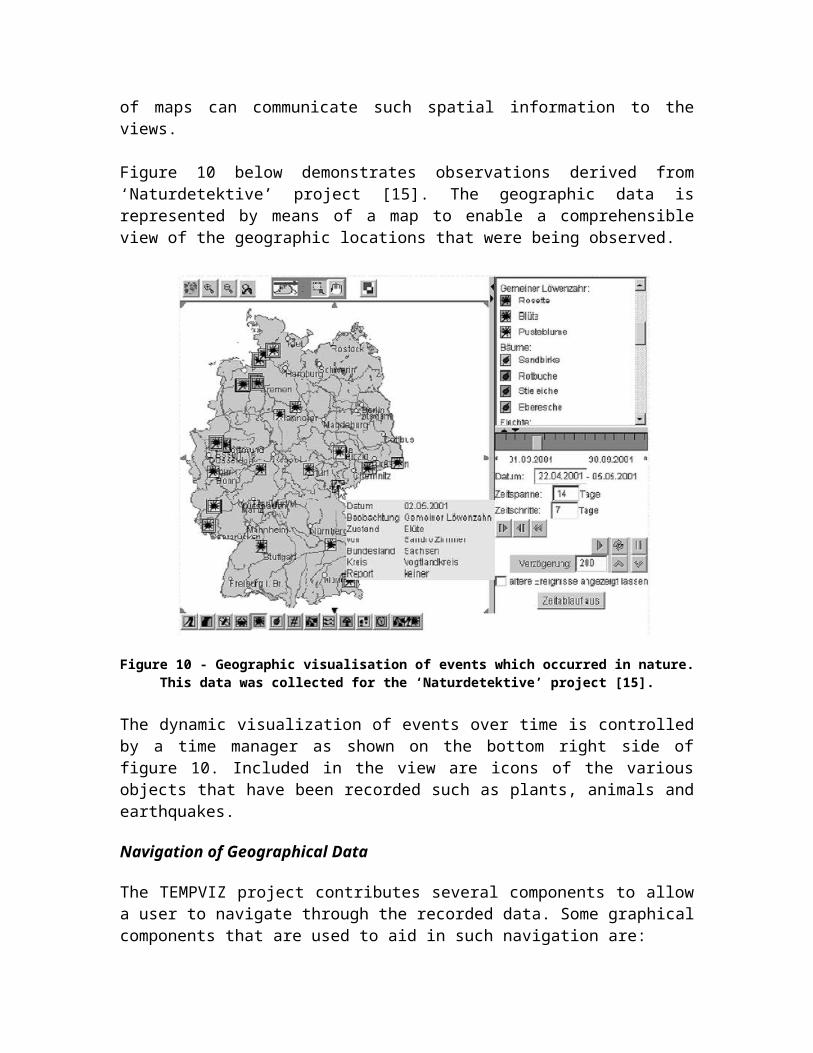
The resource package consists of the business data objects that are of interest within the application. These resources include mapping between recorded entities and Java Objects, the resources are the CPU, Task, LogFile, IPCMessage and TaskExecution. The choice to use task execution rather than task switch as business object enables more statistical information to be done. Queries such as to finding the worst-case, best-case and average-case execution time for a given task become much more direct than using task switches.

The visualization package design

SystemModel

DAOFactory«interface»

currentTime: long

TimeModel

synch()

ISynchable«interface»

ViewPart

SystemExplorer CPUGraph

SingletonSimplified UML of Visualization Plugin

Figure 19 – Simplified UML of visualization plugin package design

The UML diagram above depicts a conceptual view of the visualization tool. The diagram show two views, the SystemExplorer and CPUGraph class, both which inherit from the class ViewPart. A ViewPart is an abstract class defined in the Eclipse Platform. The latter class also implements the ISynchable interface. An ISynchable type can have an association with the TimeModel. A TimeModel instance is a collection of ISynchables and a timeline, the timeline is defined in the TimeModel. Implementers of the ISynchable interface will receive notifications when the time is modified. An ISynchable may also have a reference to the TimeModel and modify it as it sees fit. This enables loose coupling between views as they do not have to know anything about each other to synchronize the time between each other.

Layer BoundaryLayer Boundary

The SystemModel is a singleton helper object that manages access to the data access objects and the time model. In this application the SystemModel only have one TimeModel instance, implicitly making the TimeModel singleton, however the application do have support for multiple TimeModels. The DAOFactory is an instance within the DataSource layer which provides access to data access objects1.

Database Design

Figure 20 – Relationship between the entities

Figure 20 shows a E-R diagram of the database schema, the attributes of each table has intentionally been omitted for space reasons, for a full overview of the schema, see appendix A. The database consist of five tables tables, the top level item is the CPU which is identified by an ID and a Name. Next there are LogSessions, which in the prototype are log files. The name LogSession mirrors the possibility to read and save data from a netwok or from multiple files. The LogSession is also identified by an ID, a MD5 hash-checksum and a reference to a CPU. The MD5 checksum can be used to ensure that a log file has not been previously saved. A foreign key constraint CPUID refers to the one-to-many relationship between a LogSessions and its CPU. Tasks are also associated with a CPU, a row in the task table is also identified by a Id, each task can also have a

1 The Data Access Object is a design pattern to enable varying access implementation to data sources. http://java.sun.com/blueprints/corej2eepatterns/Patterns/DataAccessObject.html

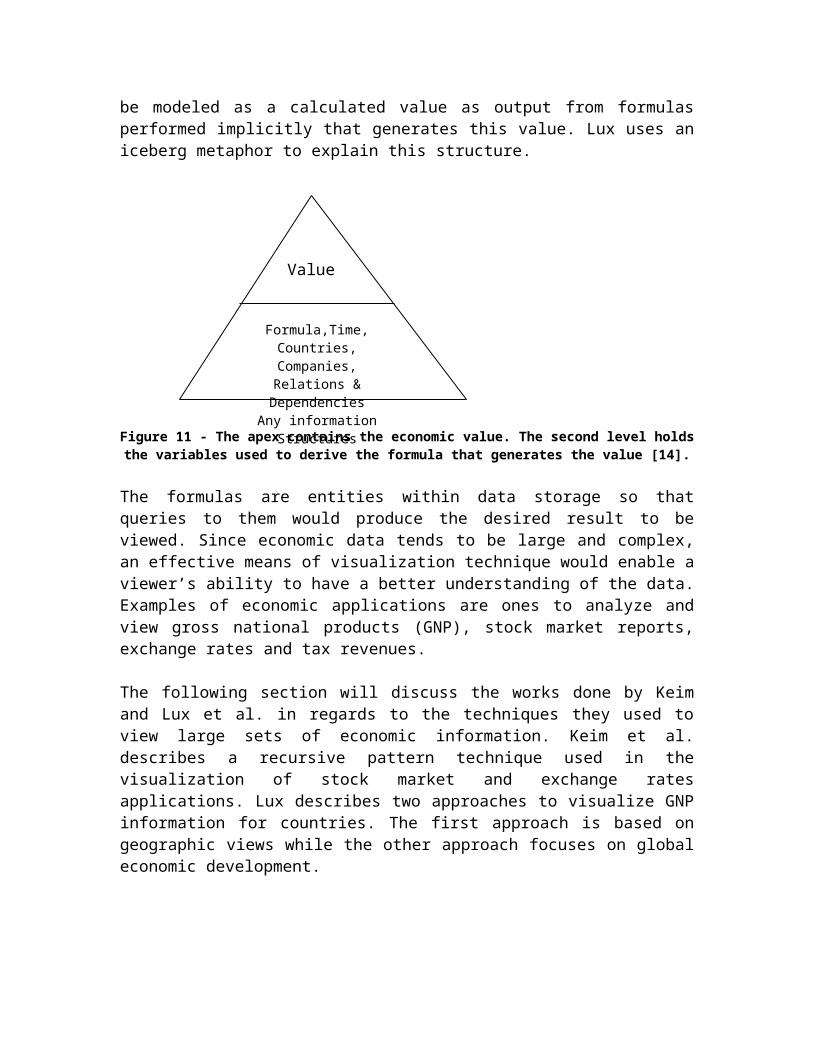
name and a task-id. The task-id is used at the CPU level and is,not guaranteed to be unique between different CPUs.

The TaskExecution table has references to which task that executes, the start and end time of the execution and which logsession the execution comes from. Storing the task-execution like this enables easy querying of min, max and average execution time of tasks. The IPCLogMessage table contains information about the time of the message, which type (typically send or receive constants), the time this message was sent, and references to the sending and receiving task. The IpcLogMessages also reference which logsession it comes from. In the case of sent messages, the EventTimestamp field and the SendTime field will be equal, however in the case of receive-type messages these fields differ, storing both these values enables quick look-up of corresponding send message for receive messages.

Using a single, atomic ID field and only atomic data within each other field, for each table in the database ensure that all tables conform to at least the second normal form2.

2 The concept of database normal forms where previously discussed under the relational databases section, p18

Suggested ViewsDrawing upon the lessons learned from other visualization areas, the basic foundation of the views presented in this thesis work will include a set of 2D views. The choice of 2D over 3D is simple, there are no maps that require a spatial region to be displayed, and 2D graphs are more readily understood over 3D graph. It is assumed that the CPUs are the top level item, where logs are associated with one CPU each. Each different view aims to help the user navigate and analyze the system. Each view has been developed with the user in mind and analyzed with the following criteria.

Information deduced – What information can be deduced using this view, why is this view useful.

Assumption – What assumptions on the underlying data model must be made for this view to function properly

Worst-case – This criteria deals with questions such as what the worst case scenario that this view must deal with as well as what can be done to minimize the impact of such a scenario.

Navigation – Similar to the information deduced, this item deals with how the user can use the view to navigate the data.

Correlation with other views – What extra connection does this view has with other views within the solution.

Possible enhancements – This item deals with how well this view scales, is there a possibility to add more advanced features.

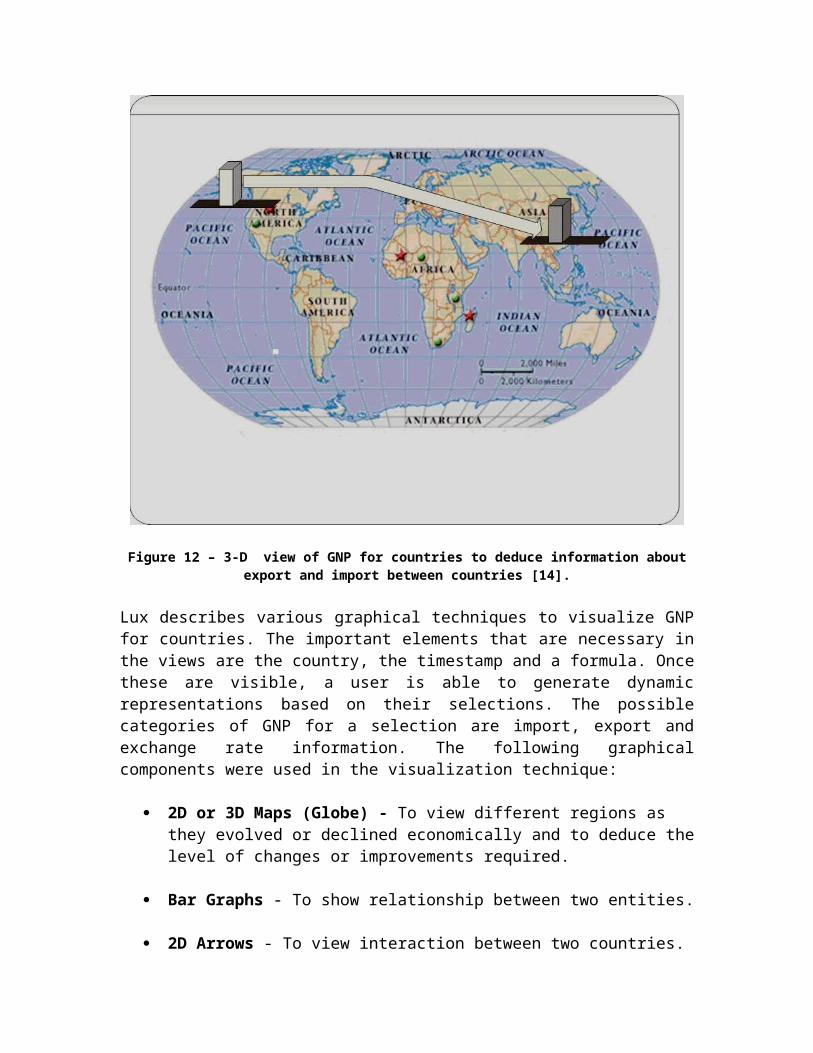
View: System Explorer

The purpose of the system explorer view is to allow the user to browse resources, including but not limited to items such as CPUs, log files and tasks. The view is similar to a file explorer, from this view it is possible to open resources in other views. This can be done by selecting a range of CPUs and through a context menu.

It is assumed that the CPUs are the top level item, where logs and tasks are associated with one CPU. The underlying data model should be able to provide a tree content provider with the system as is (the CPUs, Logs and Tasks). More so, it is also assumed that the whole content of the database represents one system and one system only. Multiple systems would then be supported by creating a new visualization project and a connecting to another database. The database may be run with the same database management server, but another database file.

At 100 CPUs there are many top level items in the hierarchy, but 100 should still be manageable by human clients. The requirement for worst-case association, 1000 logs and/or 1000 tasks under one CPU, however require attention.If the number of sub-items reaches a certain threshold, they are grouped in chunks of a more manageable size. This behaviour is already implemented in for instance the debug-view of the eclipse JDT when inspecting very large collections. The items are grouped in a tree structure in chunks of 100 items.

Figure 21 - List with many items.

As this view serves as a resource explorer and starting point for opening other visualization views, the view is not explicitly connected with the other views through the time model, however it serves as an important navigation base and is connected with the other views through their resource.

Possible enhancements include features like letting the navigator implement drag and drop functionality, to add a log to other views once they are already open.

View: CPU Graph

The CPU graph is a simple graph visualizing the behaviour of the system as it varies in time. The graph can be used to show and compare the frequency of task switches between different CPUs. From a graph it should be easy to deduce how the intensity changes in time, the information is also relative the other CPUs in the graph, the distance between the lines in the graph increases if one CPU has a higher intensity than the other.

In the worst case the view must be handle a large amount of CPUs possibly in the hundreds, this scenario is not viable as it would be hard to distinguish CPUs from each other. A small amount of CPUs may also be hard to distinguish if their graph-lines overlap i.e. has almost the same intensity.

The user can use multiple graphs to visualize a subset of the CPUs at a time, a reasonably amount may be about ten. While not necessarily limiting the graph to ten CPUs at a time, this is the preferred maximum amount; a user is able to open multiple CPU graphs. The graphs can be easily compared by placing them all in a row or a grid.

As the graph show the entire timeframe for the associated log files the navigation in time comes naturally. The graph is equipped with a vertical marker which is connected to a global time line. The marker can be moved using the mouse by clicking alternatively double clicking at some area of interest. When the user has chosen a point of interest, such as where two CPUs have a peak and double clicked at the position the global time line is updated with the time where the peak occurred. The graph is connected with other views through the global timeline, therefore any view which modifies the time line is implicitly connected with the graph and vice versa.

The graph view can be enhanced in several ways, one such enhancement over the base implementation would be to let the graph have button to change between the visualization of intensity of IPC messages and task switches, or combine them to see intensity of both. The combination would be the addition of the intensity values, if at time t0 one CPU had 5 IPC messages and 10 task switches, the intensity is now 15.

View: CPU Task Executions

This view item is a variation of a traditional Gantt chart commonly used to illustrate the executions of task on a CPU. In a traditional Gantt chart the tasks are named in a column to the left, the time is illustrated as an axis on the top or at the bottom and the executions of tasks are illustrated as a span to right of label-column. The traditional Gantt is very useful to visualize the execution of a few tasks as it clearly shows which task is currently executing, when it will be interrupted and when the next execution of the given task occurs. However the diagram does not scale well to a large amount of tasks. In the scenario common to embedded systems where there may be hundreds of task, the chart quickly becomes cumbersome to navigate. The proposed variation compresses the view to only two lanes of executions. These two lanes are shared by all tasks as they execute. This compression solves the problem of having a large number of tasks. However, we lose the direct information about the next execution of a given task. The compression of the view to two lanes also enables the view to provide a bar that visualizes IPC messages. If a task has sent or received a message this is visualized by a envelope under the task execution.

Since this view only has to deal with one CPU at a time, it does not have problems dealing with multiple CPUs. As previously explain the design overcomes the problem with a large amount of tasks as it compresses it to only two lanes. This design however comes with a limitation; it does not in an intuitive way show the next invocation of a task.

As with most other views proposed this view is linked with the global time line. Navigation in time can be done in multiple ways. A vertical time-marker like the one discussed for the CPU Graph view shows the current time. The marker can be dragged to a position of interest, for instance where a certain task starts to execute. Other navigation techniques exist such as jump to the next invocation of a task through a context menu. A context menu can also be used to jump to the corresponding send or receive of an IPC message. Being connected to the global time line the task executions view is naturally connected to all views that modify or listens to the time line.

The context menu can be used for further enhancements of the view. The menu can be used to inspect the resources such as the messages or the task. The mouse can be used to select a resource and a second view would display textual properties of the selected resource.

View: Bookmarks

While users are working with the system they may arrive at certain points at the timeline where something interesting has occurred. To allow the user to remember and efficiently navigate between such instances in time the system provides a bookmark mechanism. A bookmark can be placed with a certain timestamp along with a description. The description is user defined and allows a more memorable definition of the bookmark than just the timestamp. This view is not intended to view the actual data, rather to be able to

place and view navigational timestamp bookmarks. These bookmarks may be labelled with something interesting such as “Bad CPU-1 behaviour”.

In the worst case there may be a large amount of bookmarks, however this is up to the user to manage and is not considered a requirement at this point.This view is all about navigation. The view is implemented as a table with two columns. One column includes the timestamp associated with this bookmark, the second display the user entered label. When a row is double clicked the global time is updated with the timestamp associated with the bookmark. As previously mentioned this view is connected to the global time, and therefore any view that is connected to the global time is implicitly connected to the bookmark view.

The bookmark view can be enhanced in several ways. Bookmarks may also be labelled with some sort of severity indicator. This would make it possible sort the bookmarks by type, thus enhancing navigation. A more advanced bookmark may also save all open views and their current input, this would make it possible to retrieve the same information in another session without having to remember which views and logs were open. Lastly to ease navigation, the bookmarks could be organised in a folder-item tree structure, similar to many bookmark solutions provided by web browsers.

Result Analysis

The final result of this project will be analyzed in terms of the implemented visualization prototype created for ZealCore. The purpose of demonstrating this prototype is to enable navigation through the implemented views and analyze the behavior the tasks on the system.

As demonstrated on the left hand side of the view in figure 22 (System explorer), this prototype consists of 3 CPU’s and for each CPU there is a log session which holds the records of underlying tasks. By clicking on a log session or all the log sessions, there are options to view either a Gantt chart to view the executing tasks on a CPU or the intensity graph of the CPU across time. Figure 22 illustrates both the Gantt chart and CPU intensity graph for all three CPUs. The components included in the Gantt chart are the time marker, green and blue bars which represents the executing tasks and envelop images with arrows to show which task is sending and/or receiving a message.

Figure 22 – Visualization prototype consisting of the System Explorer, Gantt Charts, CPU Intensity Graph and Bookmarks.

The time marker is movable by a user to navigate through time to a desired time and its corresponding task. The time marker is also connected to a global time which enables synchronization with the CPU intensity graph view. When the time marker of the CPU

intensity graph is moved to a certain time, all the other markers for the other Gantt charts are updated to the show the time range as the graph marker. When this occurs, a viewer is able to note the intensity level of task executions for that time period from the graph. The graph view may also be zoomed in or out so that the viewer may get a clearer view of intensity at a period in time. From the Gantt charts, the activities for the CPU is observed such as the amount of task switches including tasks involved in IPC within the CPU.

Figure 23 – CpuTaskEditor: All instances of a selected task is represented as a clear bar;

As shown in figure 24, when a task bar is clicked once, we can see other instances of its next executions in time as they are all represented with a clear bar so it differs from the other tasks highlighted in blue and green. The color distinction allows a viewer to have a clearer view of the other task instances. Since only certain number of task executions can be viewed on the screen at once, the context menu shown in figure 24 provides the options of moving to the next or previous task invocations.

Figure 24 – CpuTaskEditor: Options to move to the previous and next instance of the selected task’s execution.

The Goto Next and Goto Previous options move the time marker to the next and previous instance of a task respectively. By using a time marker, the viewer is able to confirm the task by its id. This form of navigation is effective and faster for a user who only wants to view the behavior of one task’s execution. Moving the marker manually in search of the entire task’s instances will not only take longer, it may prove to be confusing for the user since there are so may task executions.

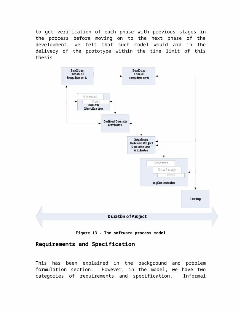
Figure 25 – CpuTaskEditor: IPC information about a selected task.

By clicking on the envelop label for a task execution, we can view the icon containing the notes about the characteristic of the task which includes the following:

The task event which is an IPC The date and time for which the task is active S: indicates the id of the task that is sending a message. R: indicates the id of the task that is receiving the sent meassage.

As illustrated in figure 26, the notes about the task 10409 show that it is sending a message to a receiving task of id 10422. By clicking on the notes, the marker jumps to where the receiving task executes. Suppose the marker jump to the instance of Task 10422 but according to its notes, the sender task is not task 10409, this can be noted as a fault in the IPC of the tasks. Such misbehavior can be bookmarked in the area on the right side of figure 26 so that the time and message is stored for a user’s knowledge about the particular tasks.

Figure 26 – Bookmarks: Text inserted in the dialogue box on the right is viewed in the ’Note’ column so that the global time is updated in the corresponding ’Time’ column.

Since the bookmark is synchronized with the global time, the process of inserting a note for a bookmark simply involves choosing from the context menu, the option to insert a note. When inserted into the pop up dialogue, it is displayed in the note column of the bookmark view. The

corresponding time column is then automatically updated with the current time to correspond with the time marked in the Gantt chart and graph.

The visualization prototype enables the ease of navigation through the views leading to the comprehension of the systems being analyzed. This is supported by the filtering technique incorporated to enable the following:

The ability to view the graph and Gantt chart for one log session at a time as opposed to viewing all the logs at the same time. This is possible due to the hierarchical structure of the system explorer.

The ability to view information about one task execution from each view of a log session’s Gantt chart. From the illustration in figure c, the execution of a selected task can be monitored by using the ‘Goto’ to step to the next or previous invocations of the tasks. When selected all instances of the task is highlighted to distinguish it from other tasks.

The visualization tool is developed in a manner that requires minimal training for a user to be able to navigate and understand the systems behaviour.

BenchmarkingRecording events from real-time systems may yield an enormous amount of events; depending on what you record there may be up to 50,000 events per second, or more. To find out whether it would be possible to record such a system from a network directly to the database via the application a benchmarking session has been run. The benchmark consists of a number of testcases with a fixed number of events inserted into the database. These figures are interesting for two reasons. The first to see if direct-recording is feasible; the second reason is to see what delay a user would experience with importing a file into the database. A user may not wish that his tool takes an excessive amount of resources compared to the specialized file-format of the native log. The following figures were recorded by benchmarking the client application against the FirebirdSQL database. The benchmarks were run on a Pentium 4 3.0 GHz with 1024MB RAM using Windows XP Pro. Each test case is run separately, before each test case the database is deleted and a new one is set up, each testcase is then run 10 times and the median value is chosen. While running a normal Windows distribution there are many possible interfering programs, which is why all tests are ran under the same conditions, with as many background tasks shutdown as possible.

Test-case with 10 tasks

Number of Events time (ms) events/ssize (kb)

size/event (kb)

1000 703 1422 1380 1,3810000 4797 2085 2168 0,2168

100000 40308 2481 11300 0,113

Table 4 – Test-case with 10 tasks

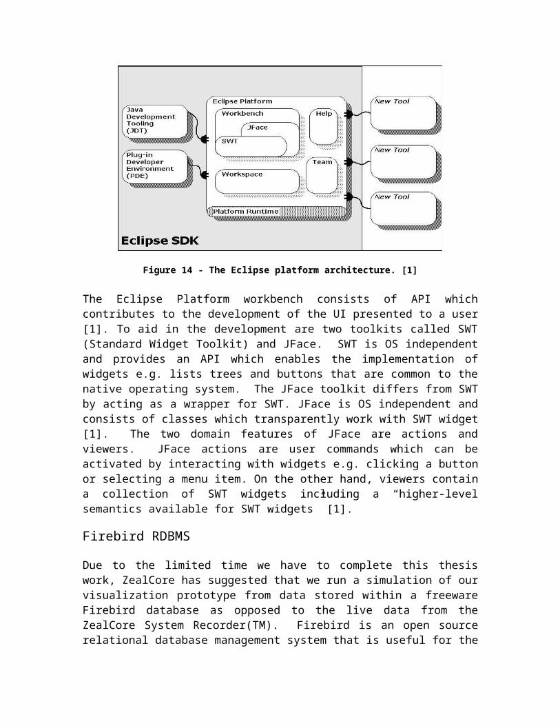
Test-case with 100 tasks

Number of Events time (ms) events/ssize (kb)

size/events (kb)

1000 765 1307 1380 1,3810000 4702 2127 2168 0,2168

100000 77689 1287 11076 0,11076

Table 5 – Test-case with 100 tasks

Test-case with 1000 tasks

Number of Events time (ms) events/s size (kb)size/events (kb)

1000 1469 681 1380 1,3810000 5390 1855 2168 0,2168

100000 80121 1248 11112 0,11112

Table 6 – Test-case with 1000 tasks

What is noticeable from the figures above is that there are no conclusive differences between the figures while inserting 10,000 events, this may be due to differences in the distribution of events, some files contains more task switches and others more IPC messages. When comparing figures for the 100,000 event files there is however a significant difference between the 10-task test compared to the 1000-task test. The difference between the 1000-task test and the 100-task test however is not as conclusive.

What can be said here is that the number of relations and the number of possible values (rows in the referenced relation) do impact on the performance of the database. Having foreign key-constraints in the events requires the database to do a lookup and check that there actually is such an element. While this ensures database integrity, it has a performance penalty. What is also interesting is that there seem to be absolutely no size difference when using 10 tasks compared to using 1000 tasks, this should be due to the task-table allocating a minimum size for the table of one database-page, in which all 1000 tasks fit in. The size of the tables is a significant factor. The database seems to require more than 100 bytes per event which would result in an enormous space expansion compared to the binary form. Events in the binary form can be very small and measured in just a few bytes3. A size expansion is expected, but with such a major factor, it may not be justified.

3 The event size of ABB Robotics trace-recording is 6 bytes in its binary form. 2006-10-27

Conclusions and Future WorkZealCore is currently undertaking an ambitious effort to develop an application based on the lessons learned from this thesis. This project will have to solve problems in areas such as the speed of reading logfiles, large databases and how to interpret arbitrary binary files. The data should also be prepared for deeper analysis. The analyses that is most straightforward and that do provide valuable information include worst-case execution, best-case execution, average execution time and fragmentation (how many times a task has been interrupted). To include this information there must be a way to know when a task starts and when it ends, it is not enough to just record task-switches. The solution is to add log information to the task-switches that tell the file interpreter which state the out-task will be in after the switch.

The analysis may also be used for profiling systems over a large time-period, this can be useful to describe how different software improves or degrade, for instance how CPU utilization or memory usage changes from release to release. Such information can be important to pin-point where bottlenecks in the system are, or if the new software version requires new hardware. The analysis portion of the application could either be implemented as the current two-tiered client-server architecture, or a three-tiered architecture. The three tiered architecture could help abstracting the intrinsic complexity of analysis as well as help easily distribute new features to all clients by only upgrading the server software. The difference in context in which the tool is used in regard s of visualization of data and data analysis suits a three tiered solution well. The visualization part should use the two tiered architecture, and the analysis part use a three-tiered architecture. By not solving the two problems together, the problem can be divided into more specialized forms for each task.

In considering the visualization part of the project many of the lessons learned in this thesis should prove useful, as an example it is recommended not only to implement the single-line Gantt chart but rather implement the second compact level of the Gantt chart mentioned in the suggested views section. Future work should also benefit from storing task-switches along with the derived TaskExecution resource. It is evident that visualization with figures provides a better understanding of a system than browsing through text files or even worse, looking at binary files with a hex editor.

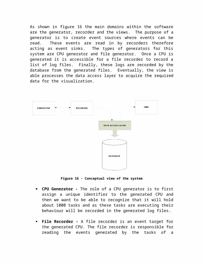
References

[1] Beaton Wayne, Eclipse Platform Technical Overview, The Eclipse Foundation, 2006.http://www.eclipse.org/articles/Whitepaper-Platform-3.1/eclipse-platform-whitepaper.html#N10125

[2] O'Sullivan Carol and Scopigno R., Graphics and Visualization: Breaking New Frontiers, Computer Graphics and Visualization found in ERCIM News No.44, January 2001.

[3] De Floriani Leila., Magillo P, and Puppo E., Multiresolution Modelling of Surface and Volume Data, Computer Graphics and Visualization found in ERCIM News No.44, January 2001.

http://www.ercim.org/publication/Ercim_News/enw44/intro.html

[4] König Andreas H. and Gröller E., 3D Medical Visualization: Breaking the Limits of Diagnostics and Treatment, Computer Graphics and Visualization found in ERCIM News No.44, January 2001

[5] STATISTICA. “Representative Visualization Techniques” found in the Online Electronic Statistics Textbook, StatSoft Inc. 2003. http://www.statsoft.com/textbook/stgraph.html#categorized12

[6] Jakob Nielsen, Alertbox – 2D is better than 3D [Internet] 1998 Nov 15, [cited 2006 Sep 10]. http://www.useit.com/alertbox/981115.html

[7] Jensen, E. Douglas and Binoy Ravindran, Eds., Asynchronous Distributed Real-Time Systems, IEEE Transactions on Computers, August 2002.

http://www.real-time.org/asyncsync.htm

[8] Thane H. Monitoring, Testing and Debugging of Distributed Real-Time Systems. Doctoral Thesis, Mälardalen Real-Time Research Centre, Mälardalen University, May 2000.http://www.mrtc.mdh.se/publications/0242.pdf

[9] Lauterbach GmbH JTAG Debugger for V850 [Internet]. 2006. http://www.lauterbach.com/frames.html?bdmv850.html

[10] Green Hills Software Inc.- SuperTrace Probe [Internet]. 2006 http://www.ghs.com/products/supertraceprobe.html

[11] Biswas Sarmistha, A Conceptual Design for Visualisation of Spatio-

temporal Data using Animation with Linked Graphics, Masters Thesis, International Institute for Geo-information Science and Earth Observation, December 2004.

[12] M. E. Shobaki. On-chip monitoring of single- and multiprocessor hardware real-time operating systems. In 8th International Conference on Real-Time Computing Systems and Applications. IEEE, March 2002.

[13] Ankerst, M., Keim, D. A.,and Kriegel, H.-P. Recursive pattern: A technique for visualizing very large amounts of data. In Proc. Visualization ’95, Atlanta, GA (1995), pp. 279–286.

[14] Keim, “Visualization of Financial Data”

[15] Andrienko Natalia, Andrienko Gennady and Gatalsky Peter, Data and Task Characteristics in Design of Spatio-Temporal Data Visualization Tools, Symposium on Geospatial Theory, Processing and Applications, Ottawa 2002.

[16] Tokuda et al. “Monitoring of Distributed Systems”

[17] E. F. Codd. A Relational Model of Data for Large Shared Data Banks. Communications of the ACM, Vol. 13, No. 6, June 1970, pp. 377-387.

[18] Ramez Elmasri, Shamkant B. Navathe. Fundamentals of database systems, second edition, 1994 ISBN 0-8053-1748-1.

[19] Shari Lawrence Pfleeger. Software Engineering – Theory And Practice, second edition, 2001 ISBN 0-13-029049-1.

[20] Wikipedia contributors. Database normalization [Internet]. Wikipedia, The Free Encyclopedia; 2006 Nov 18, 05:45 UTC [cited 2006 Nov 20]. Available from: http://en.wikipedia.org/w/index.php?title=Database_normalization&oldid=88574341.

[21] Wikipedia contributors. Database [Internet]. Wikipedia, The Free Encyclopedia; 2006 Nov 16, 14:01 UTC [cited 2006 Nov 20]. Available from: http://en.wikipedia.org/w/index.php?title=Database&oldid=88203845.

[22] Erich Gamma, Richard Helm, Ralph Johnson, John Vlissides. Design Patterns – Elements if Resusable Object-Oriented Software, 1995 ISBN 0201633612.

[23] Darleen Sadoski, GTE. Client/Server Software Architectures – An Overview [Internet]. Carnegie Mellon, Software Engineering Institute, 1997 Aug 2 [cited 2006 Nov 20]. Available from http://www.sei.cmu.edu/str/descriptions/clientserver_body.html.

Appendix A – Firebird SQL TablesCPU

ID INTEGER Not NullNAME VARCHAR(255) Not NullCONSTRAINT INTEG_43:

Primary key (ID)

LOGSESSIONID INTEGER Not NullMD5 VARCHAR(255) Not NullCPUID INTEGER Not NullCONSTRAINT FK749BDED266EE5087:

Foreign key (CPUID) References CPU (ID)CONSTRAINT INTEG_52:

Primary key (ID)

TASKID INTEGER Not NullNAME VARCHAR(255) Not NullTASKID INTEGER Not NullCPUID INTEGER Not NullCONSTRAINT FK27A9A566EE5087:

Foreign key (CPUID) References CPU (ID)CONSTRAINT INTEG_54:

Primary key (ID)

TASKEXECUTIONID INTEGER Not NullSTARTEXECUTION TIMESTAMP Not NullENDEXECUTION TIMESTAMP Not NullTASKID INTEGER Not NullLOGID INTEGER Not NullCONSTRAINT FK61278AF348200C75:

Foreign key (LOGID) References LOGSESSION (ID)CONSTRAINT FK61278AF39311E049:

Foreign key (TASKID) References TASK (ID)CONSTRAINT INTEG_60:

Primary key (ID)IPCLOGMESSAGE

ID INTEGER Not NullEVENTTIMESTAMP TIMESTAMP Not NullIPCTYPE INTEGER NullableDATA VARCHAR(255) NullableSENDTIME NUMERIC(18, 0) NullableRECIPENT INTEGER Not NullSENDER INTEGER Not NullLOGID INTEGER Not NullCONSTRAINT FK2CBCB13F48200C75:

Foreign key (LOGID) References LOGSESSION (ID)CONSTRAINT FK2CBCB13F9193051E:

Foreign key (SENDER) References TASK (ID)CONSTRAINT FK2CBCB13F979A22BD:

Foreign key (RECIPENT) References TASK (ID)CONSTRAINT INTEG_49:

Primary key (ID)