From Uncertainty to Credibility: UQ Algorithms and …€¦ · · 2014-04-04(e.g., exhibits proper ... Sample Number Base 2 Base 3 Base 5 Base 7 1 0.5000 0.3333 0.2000 0.1429

Sandia is a multiprogram laboratory operated by Sandia Corporation, a Lockheed Martin Company, for the United States Department of Energy’s National Nuclear Security Administration

under contract DE-AC04-94AL85000.

From Uncertainty to Credibility: UQ Algorithms and Research Challenges

Brian M. Adams Sandia National Laboratories

Optimization and Uncertainty Quantification

July 2, 2008

2008 CSRI Summer

Lecture SeriesSandia National Laboratories

Albuquerque, NM

Ph.D., Computational and Applied Mathematics, NC State– mathematics, statistics, computer science, immunology– nondeterministic model calibration (HIV)– internship at Fred Hutchinson Cancer Research Center

SNL since 2005 to fulfill goals:– optimization focus (surprise: uncertainty quantification) – develop algorithms; production software implementation

in DAKOTA– work with science/engineering application customers;

let their unmet needs drive research and software

Route to Sandia

Outline

• Ubiquitous computational simulation

• Why consider uncertainty quantification (UQ)

• Propagating uncertainty through models

– Intro to UQ methods

– Advanced UQ methods in DAKOTA

• Reliability-based MEMS design (OPT+UQ)

• Research challenges in electrical circuit UQ

To be credible, simulations must deliver not only a best estimate of performance, but also its degree of variability or uncertainty.

Slide credits: Mike Eldred, Laura Swiler, Barron Bichon, Genetha

Gray,

Bill Oberkampf, Matt Kerschen, others

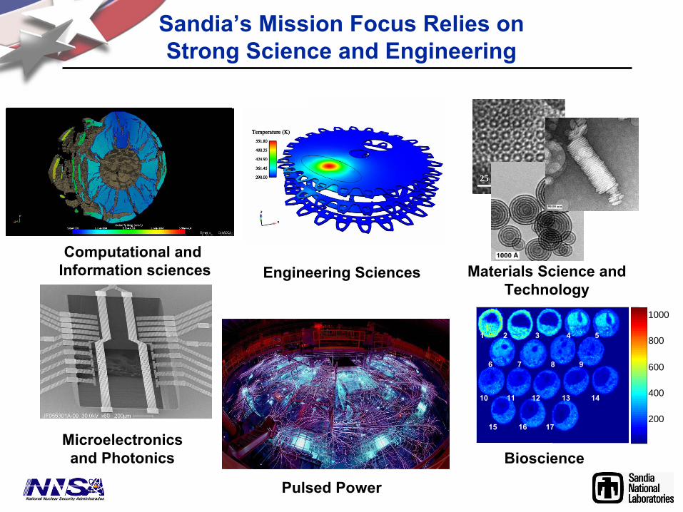
Computational andInformation sciences

Pulsed Power

Bioscience

Materials Science and Technology

25 nm25 nm (100100)

Engineering Sciences

Microelectronics and Photonics

200

400

600

800

1000

1 2 3 4 5

6 7 8 9

10 11 12 13 14

15 16 17

Sandia’s

Mission Focus Relies on Strong Science and Engineering

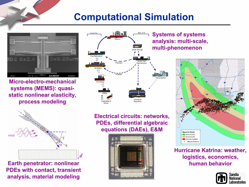
Computational Simulation

dHurricane Katrina: weather,

logistics, economics, human behavior

Electrical circuits: networks, PDEs, differential algebraic

equations (DAEs), E&M

Earth penetrator: nonlinear PDEs

with contact, transient analysis, material modeling

Micro-electro-mechanical systems (MEMS): quasi-

static nonlinear elasticity,

process modeling

Joint mechanics: system-

level FEA for component

assessment

Systems of systems analysis: multi-scale, multi-phenomenon

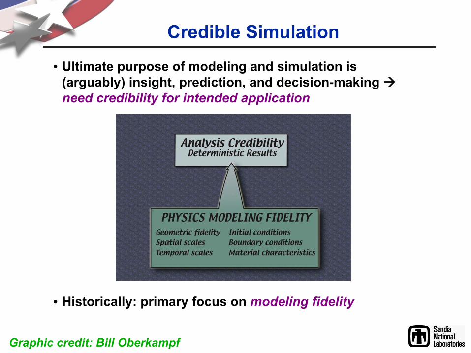
Credible Simulation

• Ultimate purpose of modeling and simulation is (arguably) insight, prediction, and decision-making need credibility for intended application

• Historically: primary focus on

modeling fidelity

Graphic credit: Bill Oberkampf

Credible Simulation: Beyond Nominal

Slide credit: Bill Oberkampf

Verification & Validation

• Verification:

“Are we solving the equations correctly?”– mathematics/computer science issue: Is our mathematical formulation

and software implementation of the physics model correct?– code verification

(software correctness); solution verification

(e.g., exhibits proper order of convergence)

• Validation –

“Are we solving the right equations?”– a disciplinary science issue: is the science (physics, biology,

etc.) model sufficient for the intended application?

Involves data and metrics.

Related concepts:• Sensitivity Analysis (SA): both local and global

– How do code outputs vary with respect to changes in code inputs?

• Uncertainty Quantification (UQ):– What are the probability distributions on code outputs, given the probability

distributions on my code inputs? Unknown input distributions?

• Quantification of margins and uncertainties (QMU):– How “close”

are my code output predictions (incl. UQ) to the system’s required performance level?

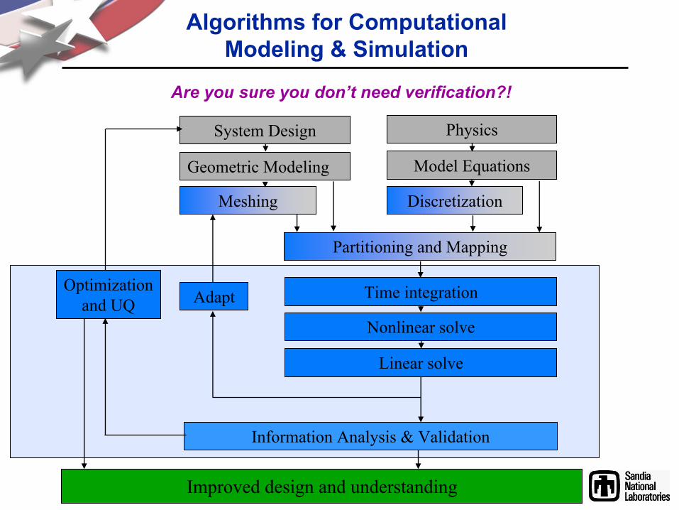
Algorithms for Computational Modeling & Simulation

System Design

Geometric Modeling

Meshing

Physics

Model Equations

Discretization

Partitioning and Mapping

Nonlinear solve

Linear solve

Time integration

Information Analysis & Validation

AdaptOptimization

and UQ

Improved design and understanding

Are you sure you don’t need verification?!

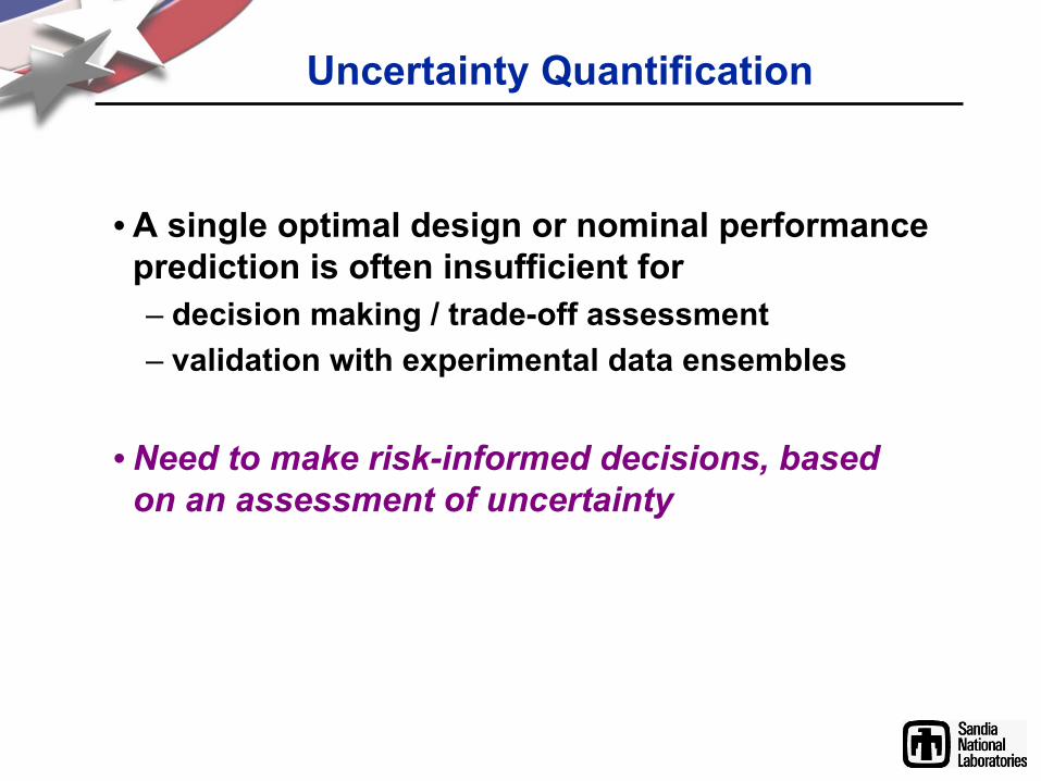
• A single optimal design or nominal performance prediction is often insufficient for – decision making / trade-off assessment– validation with experimental data ensembles

• Need to make risk-informed decisions, based on an assessment of uncertainty

Uncertainty Quantification

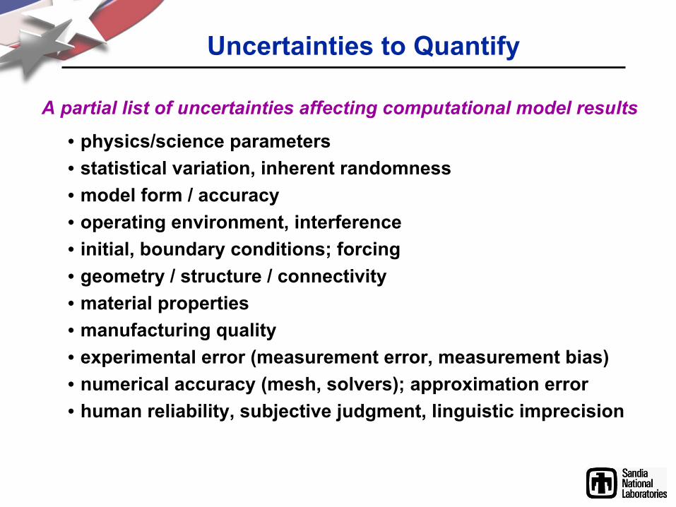
Uncertainties to Quantify

• physics/science parameters• statistical variation, inherent randomness• model form / accuracy• operating environment, interference• initial, boundary conditions; forcing• geometry / structure / connectivity• material properties• manufacturing quality• experimental error (measurement error, measurement bias)• numerical accuracy (mesh, solvers); approximation error• human reliability, subjective judgment, linguistic imprecision

A partial list of uncertainties affecting computational model results

Categories of Uncertainty

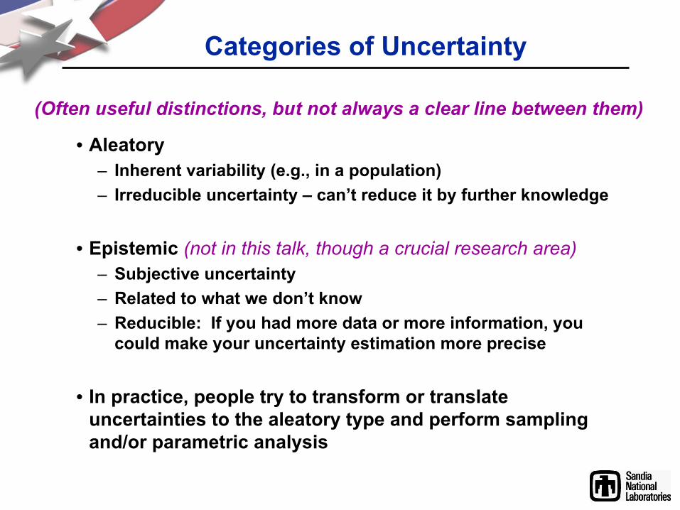
• Aleatory– Inherent variability (e.g., in a population)– Irreducible uncertainty –

can’t reduce it by further knowledge

• Epistemic (not in this talk, though a crucial research area)– Subjective uncertainty– Related to what we don’t know– Reducible: If you had more data or more information, you

could make your uncertainty estimation more precise

• In practice, people try to transform or translate uncertainties to the aleatory

type and perform sampling and/or parametric analysis

(Often useful distinctions, but not always a clear line between them)

Outline









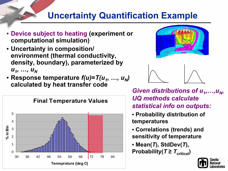
Uncertainty Quantification Example

• Device subject to heating

(experiment or computational simulation)

• Uncertainty in composition/ environment (thermal conductivity, density, boundary), parameterized by u1

, …, uN• Response temperature f(u)=T(u1

, …, uN

)

calculated by heat transfer code

Given distributions of u1

,…,uN

, UQ methods calculate statistical info on outputs:• Probability distribution of temperatures• Correlations (trends) and sensitivity of temperature• Mean(T), StdDev(T), Probability(T

≥

Tcritical

)

Final Temperature Values

0

1

2

3

4

5

30 36 42 48 54 60 66 72 78 84

Temeprature [deg C]

% in

Bin

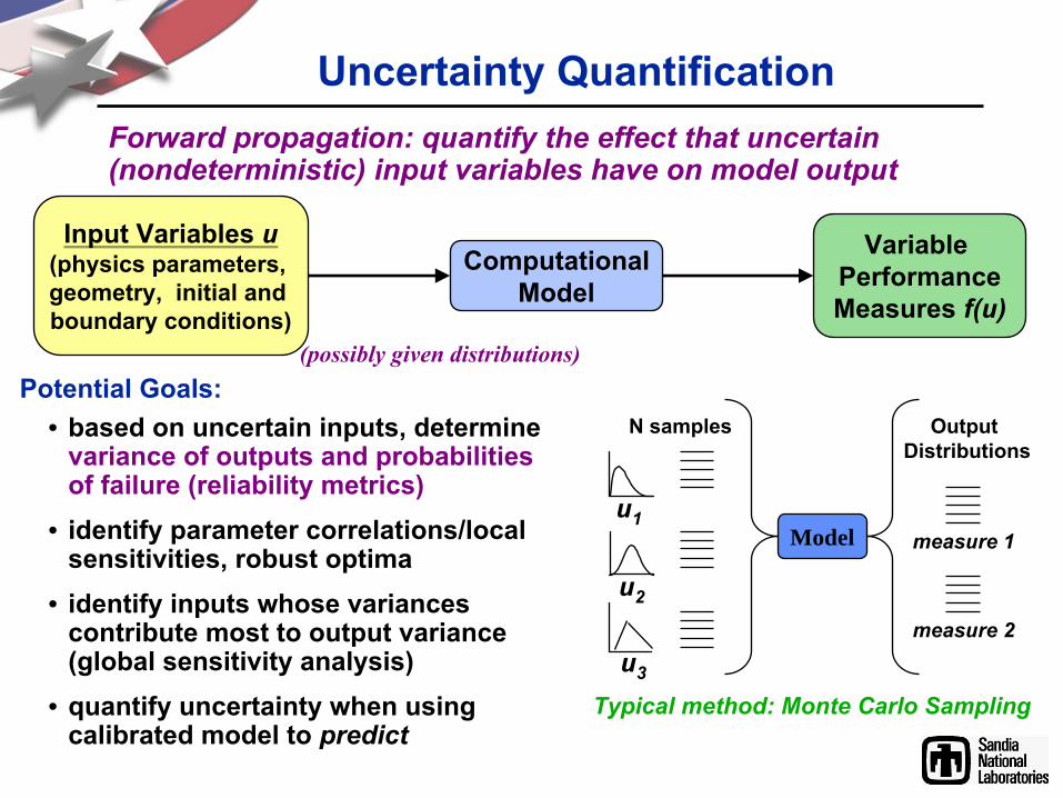
• based on uncertain inputs, determine variance of outputs and probabilities of failure (reliability metrics)

• identify parameter correlations/local sensitivities, robust optima

• identify inputs whose variances contribute most to output variance (global sensitivity analysis)

• quantify uncertainty when using calibrated model to predict

Uncertainty QuantificationForward propagation: quantify the effect that uncertain (nondeterministic) input variables have on model output

Potential Goals:

Input Variables u

(physics parameters, geometry, initial and boundary conditions)

Computational

Model

Variable Performance

Measures f(u)

(possibly given distributions)

Output Distributions

N samples

measure 1

measure 2

Model

Typical method: Monte Carlo Sampling

u1

u2

u3

0.00.20.40.60.81.0

0.40.6

0.81.0 x 1

0.20.4

0.60.8

1.01.2

x2

f(x1, x2)

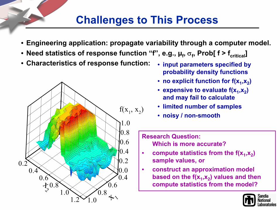
Challenges to This Process

• Engineering application: propagate variability through a computer model.• Need statistics of response function “f”, e.g., µf

, σf

, Prob[ f > fcritical

]• Characteristics of response function: • input parameters specified by

probability density functions• no explicit function for f(x1

,x2

)• expensive to evaluate f(x1

,x2

) and may fail to calculate

• limited number of samples• noisy / non-smooth

Research Question: Which is more accurate?

• compute statistics from the f(x1

,x2

) sample values, or

• construct an approximation model based on the f(x1

,x2

) values and then compute statistics from the model?

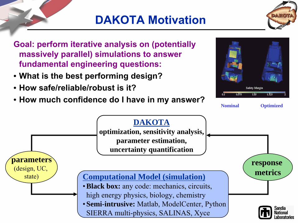
DAKOTA Motivation

Goal: perform iterative analysis on (potentially massively parallel) simulations to answer fundamental engineering questions:

• What is the best performing design? • How safe/reliable/robust is it?• How much confidence do I have in my answer?

Nominal Optimized

DAKOTA optimization, sensitivity analysis,

parameter estimation, uncertainty quantification

Computational Model (simulation)•

Black box: any code: mechanics, circuits, high energy physics, biology, chemistry

•

Semi-intrusive: Matlab, ModelCenter, Python SIERRA multi-physics, SALINAS, Xyce

response metrics

parameters (design, UC,

state)

LHS/MC

Iterator

Optimizer

ParamStudy

COLINYNPSOLDOT OPT++

LeastSqDoE

GN

Vector

MultiD

List

DDACE CCD/BB

UQ

Reliability

DSTE

JEGACONMIN

NLSSOL

NL2SOLQMC/CVT

NLPQL

Center SFEM/PCE

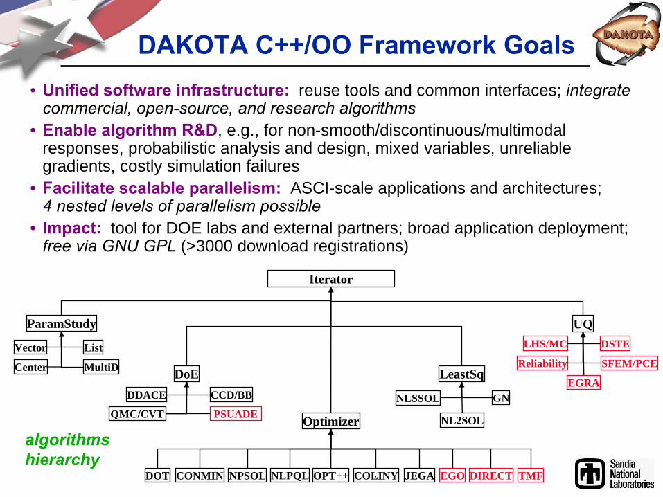
DAKOTA C++/OO Framework Goals• Unified software infrastructure:

reuse tools and common interfaces; integrate commercial, open-source, and research algorithms

• Enable algorithm R&D, e.g., for non-smooth/discontinuous/multimodal responses, probabilistic analysis and design, mixed variables, unreliable gradients, costly simulation failures

• Facilitate scalable parallelism:

ASCI-scale applications and architectures; 4 nested levels of parallelism possible

• Impact:

tool for DOE labs and external partners; broad application deployment; free via GNU GPL

(>3000 download registrations)

EGO DIRECT

algorithms

hierarchy

TMF

PSUADE

EGRA

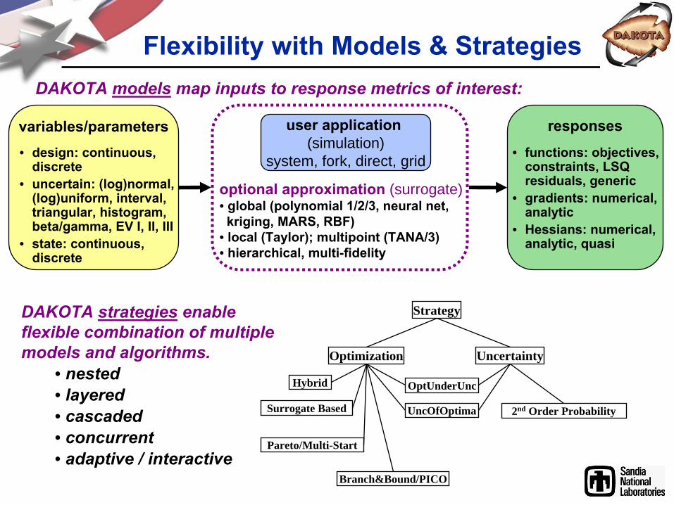
responsesvariables/parameters

Flexibility with Models & Strategies

• functions: objectives, constraints, LSQ residuals, generic

• gradients: numerical, analytic

• Hessians: numerical, analytic, quasi

user application (simulation)

system, fork, direct, grid

optional approximation

(surrogate)• global (polynomial 1/2/3, neural net, kriging, MARS, RBF)

• local (Taylor); multipoint (TANA/3)• hierarchical, multi-fidelity

• design: continuous, discrete

• uncertain: (log)normal, (log)uniform, interval, triangular, histogram, beta/gamma, EV I, II, III

• state: continuous, discrete

DAKOTA strategies

enable flexible combination of multiple models and algorithms.

• nested• layered• cascaded• concurrent• adaptive / interactive

Hybrid

Surrogate Based

OptUnderUnc

Branch&Bound/PICO

Strategy

Optimization Uncertainty

2nd Order ProbabilityUncOfOptima

Pareto/Multi-Start

DAKOTA models

map inputs to response metrics of interest:

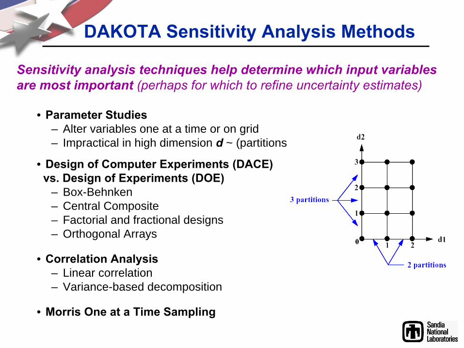
DAKOTA Sensitivity Analysis Methods

• Parameter Studies– Alter variables one at a time or on grid– Impractical in high dimension d

~ (partitions)d

• Design of Computer Experiments (DACE)vs. Design of Experiments (DOE)

– Box-Behnken– Central Composite– Factorial and fractional designs– Orthogonal Arrays

• Correlation Analysis– Linear correlation– Variance-based decomposition

• Morris One at a Time Sampling

Sensitivity analysis techniques help determine which input variables are most important (perhaps for which to refine uncertainty estimates)

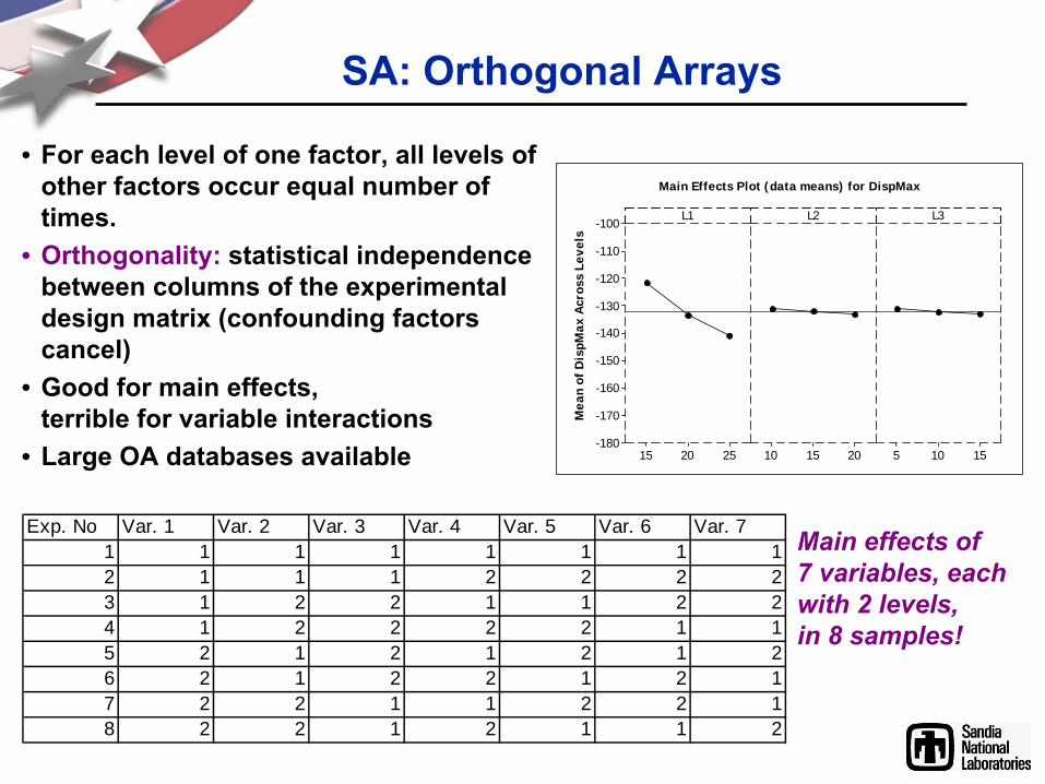
SA: Orthogonal Arrays

• For each level of one factor, all levels of other factors occur equal number of times.

• Orthogonality:

statistical independence between columns of the experimental design matrix (confounding factors cancel)

• Good for main effects, terrible for variable interactions

• Large OA databases available

Exp. No Var. 1 Var. 2 Var. 3 Var. 4 Var. 5 Var. 6 Var. 71 1 1 1 1 1 1 12 1 1 1 2 2 2 23 1 2 2 1 1 2 24 1 2 2 2 2 1 15 2 1 2 1 2 1 26 2 1 2 2 1 2 17 2 2 1 1 2 2 18 2 2 1 2 1 1 2

Mea

n of

Dis

pMax

Acr

oss

Leve

ls

252015

-100

-110

-120

-130

-140

-150

-160

-170

-180201510 15105

L1 L2 L3

Main Effects Plot (data means) for DispMax

Main effects of 7 variables, each with 2 levels, in 8 samples!

UQ: Sampling Methods

Given distributions

of u1

,…,uN

, UQ methods…


0

1

2

3

4

5

30 36 42 48 54 60 66 72 78 84

Temeprature [deg C]

% in

Bin

Output Distributions

N samples

measure 1

measure 2

Model…calculate statistical info on outputs T(u1

,…,uN

)u1

u2

u3

Quasi-Monte Carlo Sequences

• Deterministic sequences from a series of prime bases

• Designed to produce uniform random numbers on the interval [0,1]

• Low discrepancy • Example: Halton

sequences

Sample Number Base 2 Base 3 Base 5 Base 71 0.5000 0.3333 0.2000 0.14292 0.2500 0.6667 0.4000 0.28573 0.7500 0.1111 0.6000 0.42864 0.1250 0.4444 0.8000 0.57145 0.6250 0.7778 0.0400 0.71436 0.3750 0.2222 0.2400 0.85717 0.8750 0.5556 0.4400 0.02048 0.0625 0.8889 0.6400 0.16339 0.5625 0.0370 0.8400 0.306110 0.3125 0.3704 0.0800 0.4490

Base 2 and Base 3

0

0.1

0.2

0.3

0.4

0.5

0.6

0.7

0.8

0.9

1

0 0.1 0.2 0.3 0.4 0.5 0.6 0.7 0.8 0.9 1

Halton 100 pointsHalton 25 pointsHalton 10 points

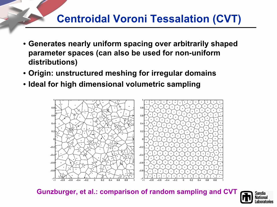
Centroidal

Voroni

Tessalation

(CVT)

• Generates nearly uniform spacing over arbitrarily shaped parameter spaces (can also be used for non-uniform distributions)

• Origin: unstructured meshing for irregular domains • Ideal for high dimensional volumetric sampling

Gunzburger, et al.: comparison of random sampling and CVT

0.2 0.2 0.2 0.2 0.2

A B C D−∞ ∞

0

0.2

0.4

0.6

0.8

1

A B C D−∞ ∞

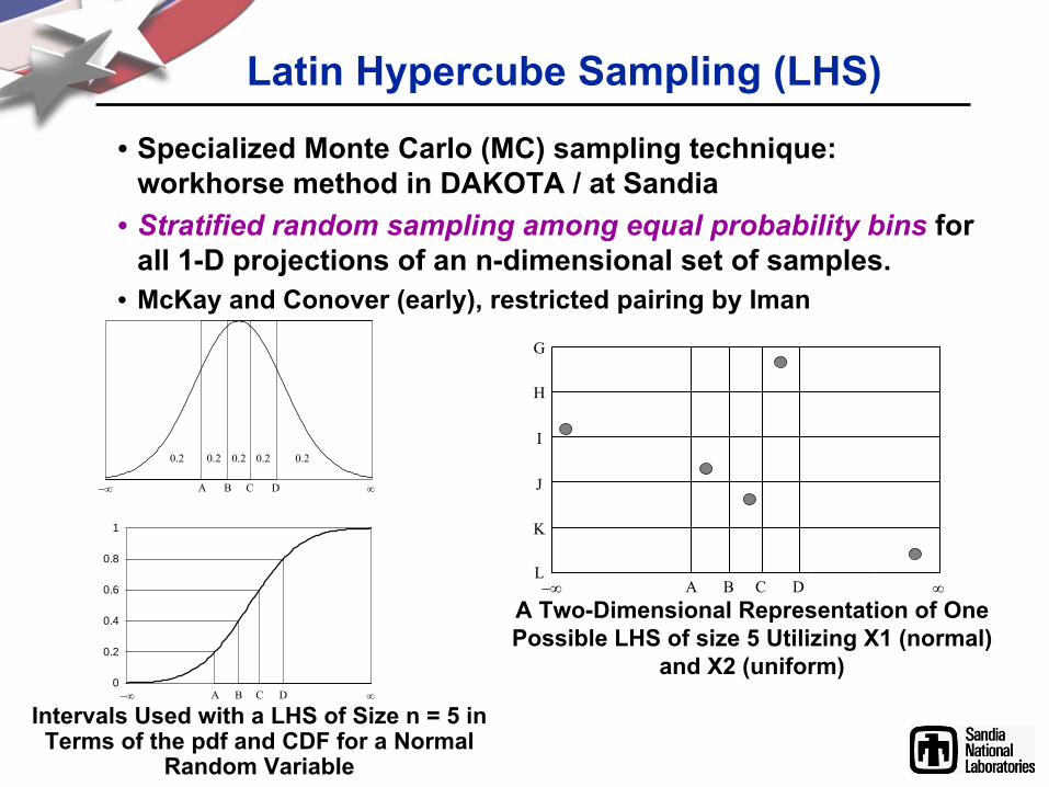
Latin Hypercube Sampling (LHS)

• Specialized Monte Carlo (MC) sampling technique: workhorse method in DAKOTA / at Sandia

• Stratified random sampling among equal probability bins

for all 1-D projections of an n-dimensional set of samples.

• McKay and Conover (early), restricted pairing by Iman

A B C D

G

H

I

J

K

L−∞ ∞

Intervals Used with a LHS of Size n = 5 in Terms of the pdf

and CDF for a Normal Random Variable

A Two-Dimensional Representation of One Possible LHS of size 5 Utilizing X1 (normal)

and X2 (uniform)

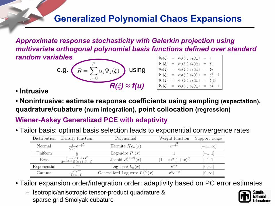
Approximate response stochasticity

with Galerkin

projection using

multivariate orthogonal polynomial basis functions defined over standard

random variables

e.g. using

• Intrusive• Nonintrusive: estimate response coefficients using sampling (expectation),

quadrature/cubature (num integration),

point collocation (regression)

Wiener-Askey

Generalized PCE with adaptivity• Tailor basis: optimal basis selection leads to exponential convergence rates

• Tailor expansion order/integration order: adaptivity based on PC error estimates– Isotropic/anisotropic tensor-product quadrature &

sparse grid Smolyak cubature

Generalized Polynomial Chaos Expansions

R(ξ) ≈

f(u)

CDF

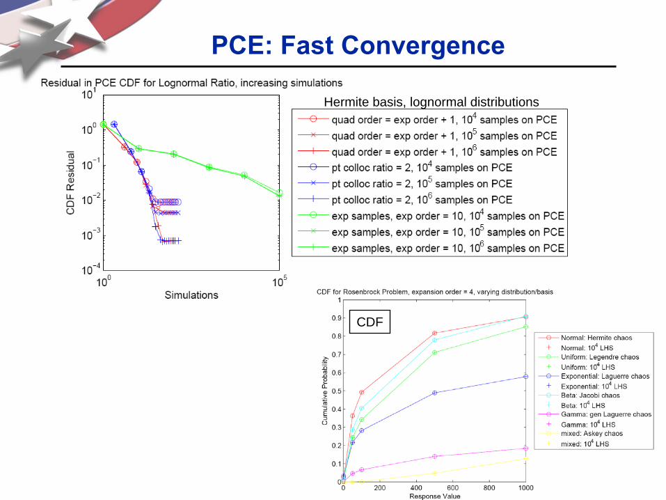
PCE: Fast Convergence

Hermite basis, lognormal distributions

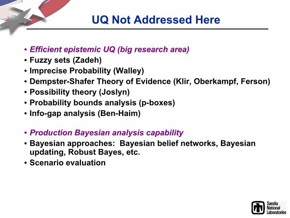
UQ Not Addressed Here

• Efficient epistemic UQ (big research area)• Fuzzy sets (Zadeh)• Imprecise Probability (Walley)• Dempster-Shafer Theory of Evidence (Klir, Oberkampf, Ferson)• Possibility theory (Joslyn)• Probability bounds analysis (p-boxes)• Info-gap analysis (Ben-Haim)

• Production Bayesian analysis capability• Bayesian approaches: Bayesian belief networks, Bayesian

updating, Robust Bayes, etc.• Scenario evaluation

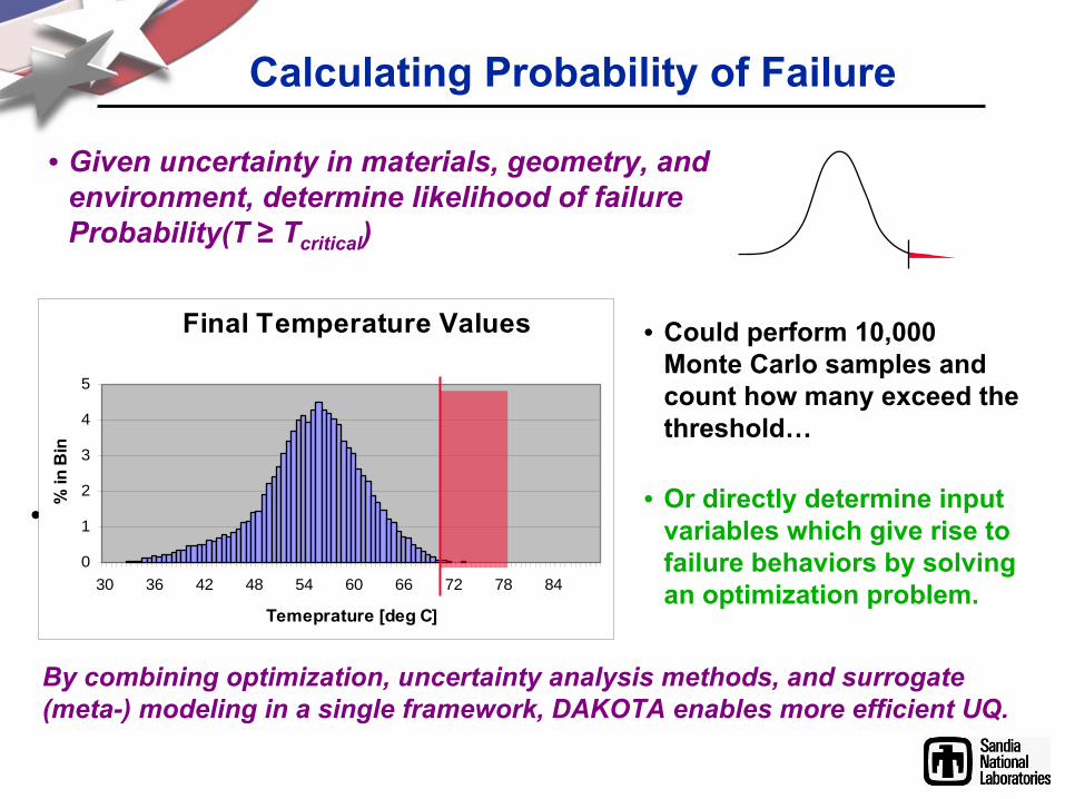
Calculating Probability of Failure

• Given uncertainty in materials, geometry, and environment, determine likelihood of failure Probability(T

≥

Tcritical

)

•


0

1

2

3

4

5

30 36 42 48 54 60 66 72 78 84

Temeprature [deg C]

% in

Bin

• Could perform 10,000 Monte Carlo samples and count how many exceed the threshold…

• Or directly determine input variables which give rise to failure behaviors by solving an optimization problem.

By combining optimization, uncertainty analysis methods, and surrogate (meta-) modeling in a single framework, DAKOTA enables more efficient UQ.

Analytic Reliability: MPP Search

Perform optimization in uncertain variable space to determine Most Probable Point (of response or failure occurring) for G(u) = T(u).

Reliability Index Approach (RIA)

G(u)

Region of u values where T ≥

Tcriticalmap Tcritical

to a probability

• Limit state linearizations: use a local surrogate for the limit state G(u)

during optimization in u-space (or x-space):

Reliability: Algorithmic VariationsMany variations possible to improve efficiency, including in DAKOTA…

• Integrations (in u-space to determine probabilities): may need higher order for nonlinear limit states

1st-order:

• MPP search algorithm: Sequential Quadratic Prog. (SQP) vs. Nonlinear Interior Point (NIP)• Warm starting (for linearizations, initial iterate for MPP searches):

speeds convergence when increments made in: approximation, statistics requested, design variables

curvature correction

2nd-order:

(could use analytic, finite difference, or quasi-Newton (BFGS, SR1) Hessians in approximation/optimization –

results here mostly use SR1 quasi-Hessians.)

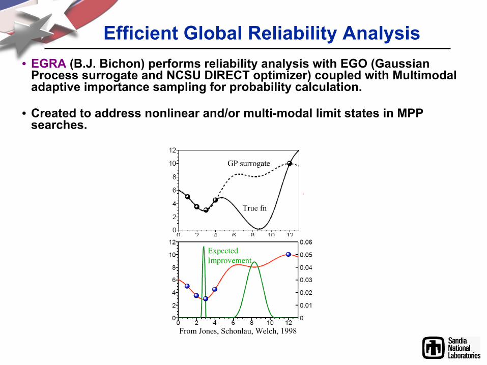
Efficient Global Reliability Analysis• EGRA

(B.J. Bichon) performs reliability analysis with EGO (Gaussian Process surrogate and NCSU DIRECT optimizer) coupled with Multimodal adaptive importance sampling for probability calculation.

• Created to address nonlinear and/or multi-modal limit states in MPP searches.

True fn

GP surrogate

Expected

Improvement

From Jones, Schonlau, Welch, 1998

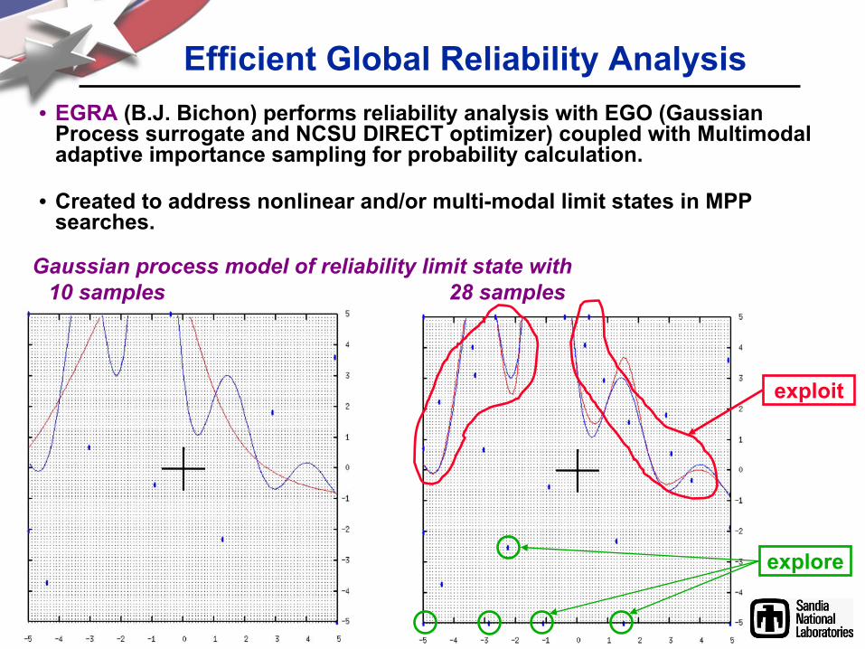
Efficient Global Reliability Analysis• EGRA

(B.J. Bichon) performs reliability analysis with EGO (Gaussian Process surrogate and NCSU DIRECT optimizer) coupled with Multimodal adaptive importance sampling for probability calculation.

• Created to address nonlinear and/or multi-modal limit states in MPP searches.

Gaussian process model of reliability limit state with

10 samples

28 samples

explore

exploit

Outline









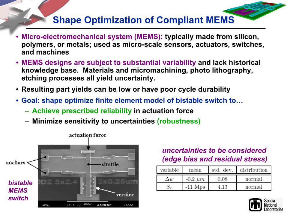
Shape Optimization of Compliant MEMS• Micro-electromechanical system (MEMS):

typically made from silicon, polymers, or metals; used as micro-scale sensors, actuators, switches, and machines

• MEMS designs are subject to substantial variability

and lack historical knowledge base. Materials and micromachining, photo lithography, etching processes all yield uncertainty.

• Resulting part yields can be low or have poor cycle durability• Goal: shape optimize finite element model of bistable

switch to…– Achieve prescribed reliability

in actuation force– Minimize sensitivity to uncertainties (robustness)

bistable

MEMS switch

uncertainties to be considered (edge bias and residual stress)

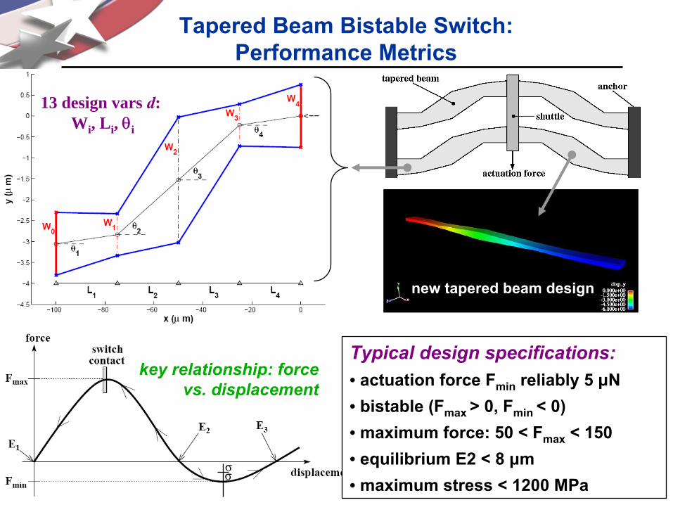
Tapered Beam Bistable

Switch: Performance Metrics

13 design vars d: Wi , Li , θi

σσ

key relationship: force

vs. displacement

new tapered beam design

Typical design specifications:• actuation force Fmin

reliably 5 μN• bistable

(Fmax

> 0, Fmin

< 0)• maximum force: 50 < Fmax

< 150• equilibrium E2 < 8 μm• maximum stress < 1200 MPa

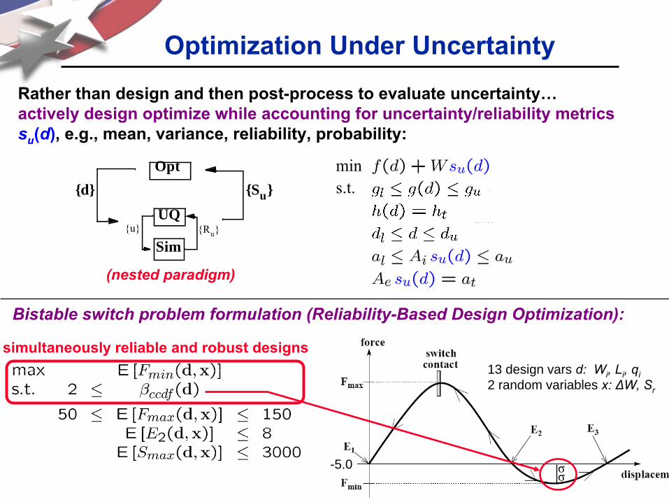
Optimization Under Uncertainty

Opt

UQ

Sim

d Su

u Ru

min

s.t.

(nested paradigm)

Rather than design and then post-process to evaluate uncertainty…

actively design optimize while accounting for uncertainty/reliability metrics su

(d), e.g., mean, variance, reliability, probability:

13 design vars d: Wi

, Li

, qi

2 random variables x: ΔW, Sr

σσ-5.0

simultaneously reliable and robust designs

Bistable

switch problem formulation (Reliability-Based Design Optimization):

min

s.t.

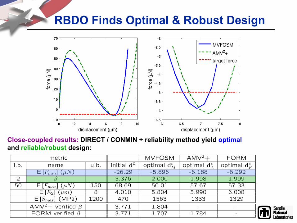
RBDO Finds Optimal & Robust Design

Close-coupled results:

DIRECT / CONMIN + reliability method yield optimal

and reliable/robust

design:

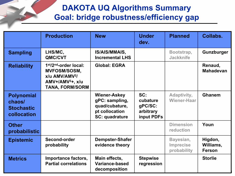
DAKOTA UQ Algorithms Summary Goal: bridge robustness/efficiency gap

Production New Under dev.

Planned Collabs.

Sampling LHS/MC, QMC/CVT

IS/AIS/MMAIS, Incremental LHS

Bootstrap, Jackknife

Gunzburger

Reliability 1st/2nd-order local: MVFOSM/SOSM, x/u

AMV/AMV2/ AMV+/AMV2+, x/u

TANA, FORM/SORM

Global: EGRA Renaud, Mahadevan

Polynomial chaos/ Stochastic collocation

Wiener-Askey

gPC: sampling, quad/cubature, pt collocation

SC: quadrature

SC: cubaturegPC/SC: arbitrary input PDFs

Adaptivity, Wiener-Haar

Ghanem

Other probabilistic

Dimension reduction

Youn

Epistemic Second-order probability

Dempster-Shafer evidence theory

Bayesian, Imprecise probability

Higdon, Williams, Ferson

Metrics Importance factors, Partial correlations

Main effects, Variance-based decomposition

Stepwise regression

Storlie

Outline









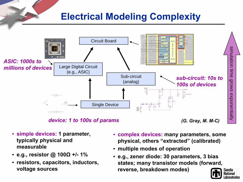
Electrical Modeling Complexity

• simple devices:

1 parameter, typically physical and measurable

• e.g., resistor @ 100Ω

+/-

1%• resistors, capacitors, inductors,

voltage sources

Circuit Board

Large Digital Circuit(e.g., ASIC)

Sub-circuit (analog)

Single Device

device: 1 to 100s of params

sub-circuit: 10s to 100s of devices

ASIC: 1000s to millions of devices

• complex devices:

many parameters, some physical, others “extracted”

(calibrated)• multiple modes of operation• e.g., zener

diode: 30 parameters, 3 bias states; many transistor models (forward, reverse, breakdown modes)

simulation tim

e grows exponentially

(G. Gray, M. M-C)

Electrical Circuit UQ

• Circuit analysis challenges– network of nonlinearly coupled components, feedback loops, staged behavior,

or discrete digital logic, mandating all-at-once circuit solution techniques– long simulation time involving iterative solvers (often hours to

simulate microseconds, particularly in oscillating electronics);

– combination of analog and digital circuits: consider separately or together• analog circuits typically < 100 devices, including replicates, less predictable topology

across designs• digital circuits 1,000 to 1,000,000 transistors (identical or similar), small number of

well-defined connection types.

• Typical parametric uncertainties:– process parameters (e.g., diffusion times, oven temperatures)– physical parameters (e.g., line widths, channel doping)– model parameters (e.g., BSIM3 transistor compact model)– electrical parameters (e.g., line resistance, saturation current, threshold

voltage)• Mapping reality to compact model parameters not always easy; compact model

may be more behavioral than physics-based

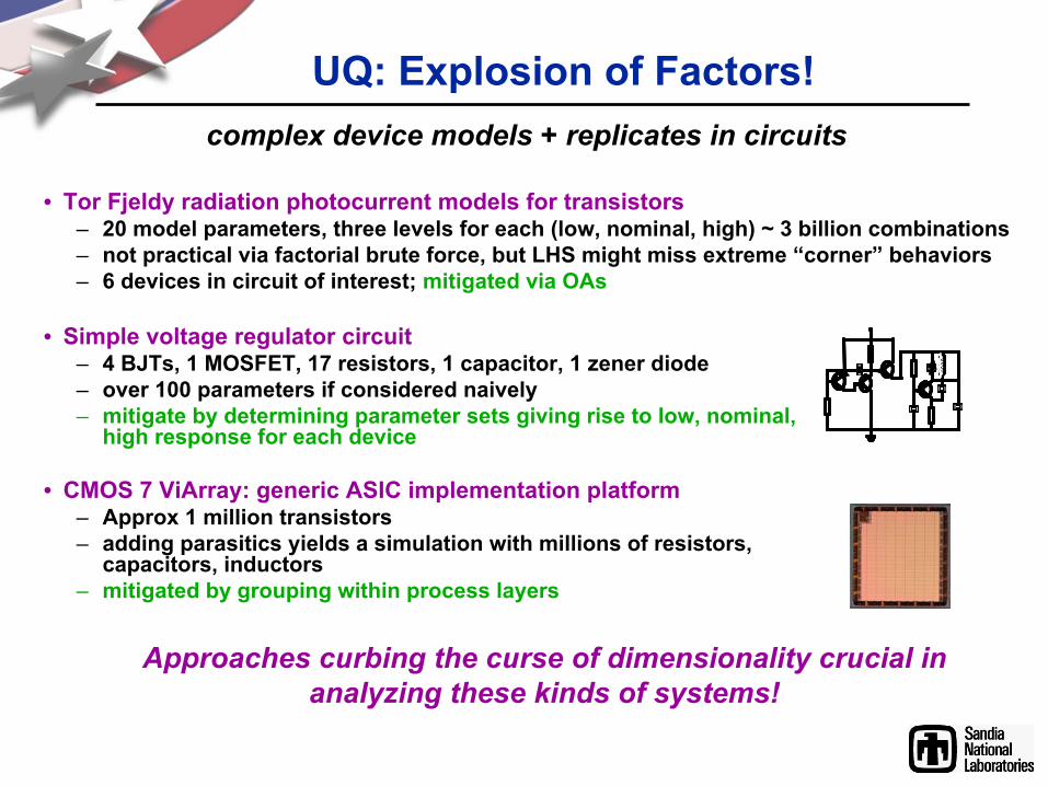
UQ: Explosion of Factors!

• Tor Fjeldy

radiation photocurrent models for transistors– 20 model parameters, three levels for each (low, nominal, high) ~ 3 billion combinations– not practical via factorial brute force, but LHS might miss extreme “corner”

behaviors– 6 devices in circuit of interest; mitigated via OAs

• Simple voltage regulator circuit– 4 BJTs, 1 MOSFET, 17 resistors, 1 capacitor, 1 zener

diode– over 100 parameters if considered naively– mitigate by determining parameter sets giving rise to low, nominal,

high response for each device

• CMOS 7 ViArray: generic ASIC implementation platform– Approx 1 million transistors– adding parasitics

yields a simulation with millions of resistors, capacitors, inductors

– mitigated by grouping within process layers

complex device models + replicates in circuits

Approaches curbing the curse of dimensionality crucial in analyzing these kinds of systems!

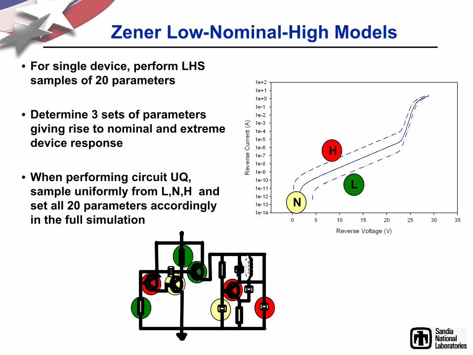
Zener

Low-Nominal-High Models• For single device, perform LHS

samples of 20 parameters

• Determine 3 sets of parameters giving rise to nominal and extreme device response

• When performing circuit UQ, sample uniformly from L,N,H and set all 20 parameters accordingly in the full simulation

L

H

N

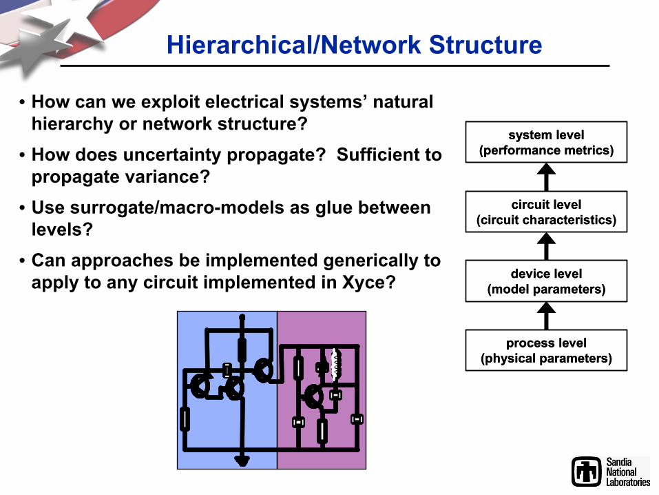
Hierarchical/Network Structure

• How can we exploit electrical systems’

natural hierarchy or network structure?

• How does uncertainty propagate? Sufficient to propagate variance?

• Use surrogate/macro-models as glue between levels?

• Can approaches be implemented generically to apply to any circuit implemented in Xyce?

process level(physical parameters)

device level(model parameters)

circuit level(circuit characteristics)

system level(performance metrics)

process level(physical parameters)

device level(model parameters)

circuit level(circuit characteristics)

system level(performance metrics)

Other Relevant Technologies

• Apply existing reliability and polynomial chaos methods; benefit of embedded techniques?

• Principal components analysis (PCA, SVD, POD), reduced-

order modeling techniques: only vary uncorrelated parameters

• Surrogate/macro modeling, insert current/voltage sources representative of the effect of uncertainty

• Leverage structure of network, DAE system under the hood; automatic structure analysis, macro-model creation?

Summary

• Uncertainty quantification algorithms are essential in credible simulation

• Complex, large-scale simulations demand research in advanced efficient UQ methods


Thank you for your [email protected]

http://www.sandia.gov/~briadam

Abstract

• 2008 CSRI Summer Lecture Series

• Title: "From uncertainty to credibility: UQ algorithms and research challenges"

• Speaker: Brian Adams (Org. 1411)

• Date/Time: Wednesday, July 2, 3-4pm (MST)

• Location:• NM: CSRI/90• CA: 915/S145

• Abstract:

• Computational simulations are routinely used to assess the performance, reliability, and safety of existing and proposed systems, and are increasingly used for risk-informed decision making in the presence of uncertainties. To be credible, simulations must deliver not only a best estimate of performance, but also its degree of variability or uncertainty.

• Uncertainty quantification (UQ) algorithms compute the effect of

uncertain input variables on response metrics of interest, enabling risk assessment, model calibration, and model

validation. In this talk, I will motivate simulation-

based UQ with examples from electrical circuit and MEMS design. I will survey methods from ubiquitous Monte Carlo sampling through more advanced reliability analysis and polynomial chaos expansions available in Sandia's

DAKOTA toolkit. In particular, DAKOTA’s

reliability analysis methods employ a mix of probability, optimization, and surrogate (meta-) modeling to efficiently perform UQ.

• Challenges in large-scale electrical circuit UQ will motivate unmet algorithm research needs.

Extra Slides

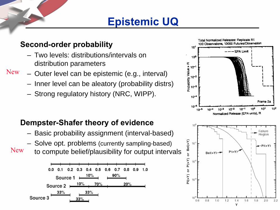
Epistemic UQ

Second-order probability– Two levels: distributions/intervals on

distribution parameters– Outer level can be epistemic (e.g., interval)– Inner level can be aleatory (probability distrs)– Strong regulatory history (NRC, WIPP).

Dempster-Shafer theory of evidence– Basic probability assignment (interval-based)– Solve opt. problems (currently sampling-based)

to compute belief/plausibility for output intervals

New

New

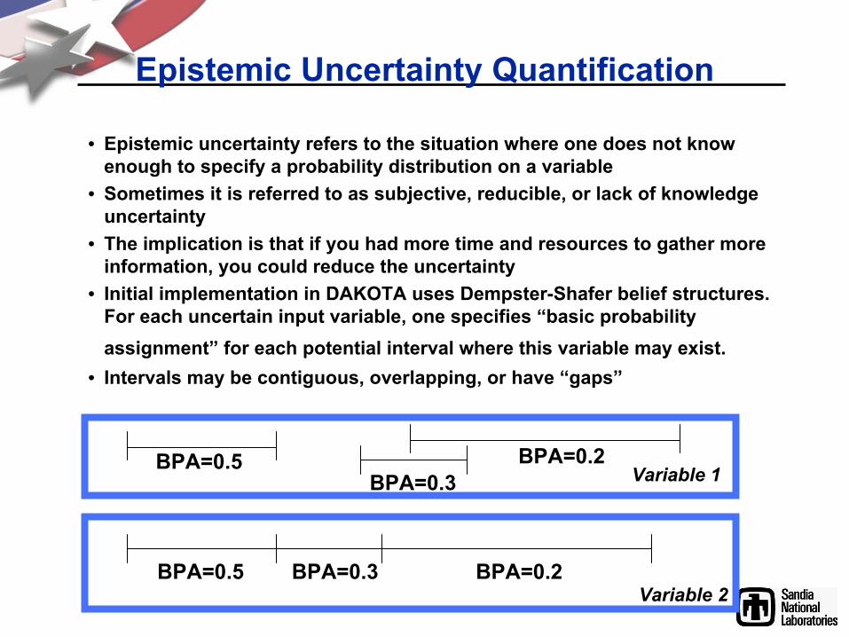
Epistemic Uncertainty Quantification

• Epistemic uncertainty refers to the situation where one does not

know enough to specify a probability distribution on a variable

• Sometimes it is referred to as subjective, reducible, or lack of

knowledge uncertainty

• The implication is that if you had more time and resources to gather more information, you could reduce the uncertainty

• Initial implementation in DAKOTA uses Dempster-Shafer belief structures. For each uncertain input variable, one specifies “basic probability assignment”

for each potential interval where this variable may exist.• Intervals may be contiguous, overlapping, or have “gaps”

BPA=0.5 BPA=0.2BPA=0.3 Variable 1

BPA=0.5 BPA=0.2BPA=0.3Variable 2

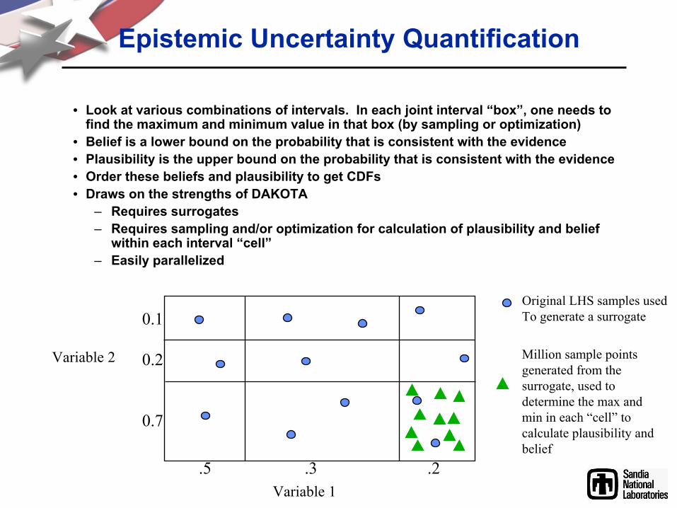
Epistemic Uncertainty Quantification

• Look at various combinations of intervals. In each joint interval “box”, one needs to find the maximum and minimum value in that box (by sampling or optimization)

• Belief is a lower bound on the probability that is consistent with the evidence• Plausibility is the upper bound on the probability that is consistent with the evidence• Order these beliefs and plausibility to get CDFs• Draws on the strengths of DAKOTA

– Requires surrogates– Requires sampling and/or optimization for calculation of plausibility and belief

within each interval “cell”– Easily parallelized

Variable 1

Variable 2

.5

.3

.2

0.1

0.2

0.7

Original LHS samples used To generate a surrogate

Million sample points generated from the surrogate, used to determine the max and min in each “cell”

to calculate plausibility and belief

Bayesian Analysis

• Construct a prior distribution on a parameter (which might be a parameter of a distribution)

• The prior distribution should be based on previous experience, engineering judgment

• The distribution on the prior is updated with actual data. The resulting updated distribution is called the posterior. Frequentist Bayesian

Assumes there is an unknown but fixed parameter θ

Assumes a distribution on unknown parameter θ

Estimates θ

with some confidence interval

Uses probability theory, treats θ

as a random variable

Bayesian Analysis

• Why would we use it for CS&E problems? • Nice feature of incorporating additional data as it becomes

available• We often don’t have good estimates: Bayes provides a

framework for starting with what we do know, and refining our estimates in a statistically consistent manner

• Examples:– Reliability problems: Update probability of failure– Response surfaces: Update parameters in a surrogate

model for a trust region– Calibration under Uncertainty (CUU): Update our parameter

estimates based on experimental data AND uncertainty in a model

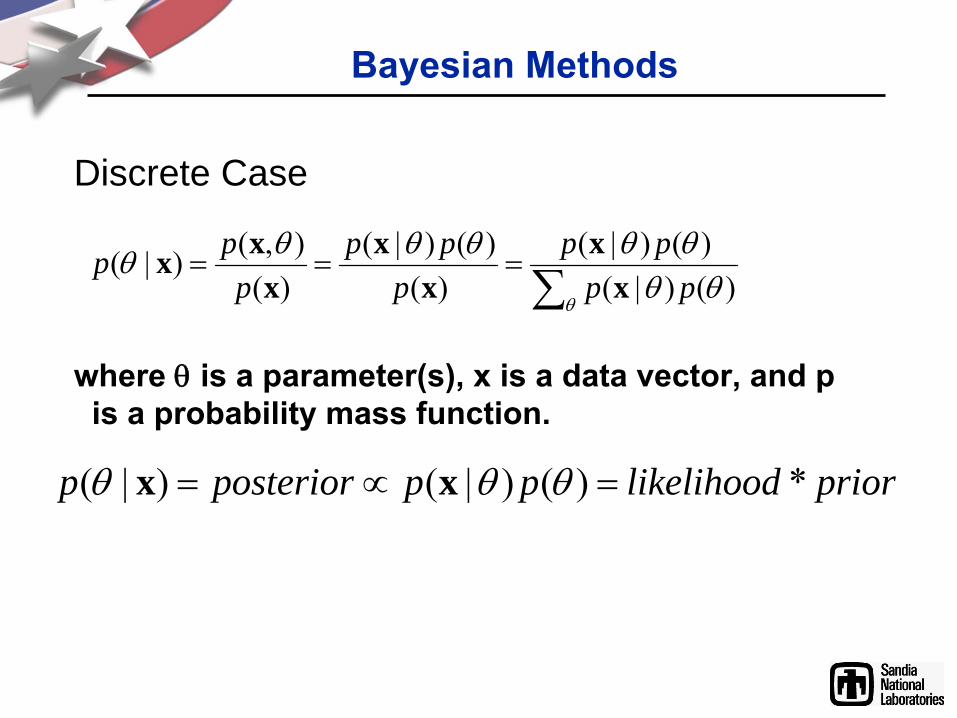
Bayesian Methods

Discrete Case

where θ

is a parameter(s), x is a data vector, and p is a probability mass function.

∑===

θθθ

θθθθθθ)()|(

)()|()(

)()|()(),()|(

pppp

ppp

ppp

xx

xx

xxx

priorlikelihoodppposteriorp *)()|()|( =∝= θθθ xx

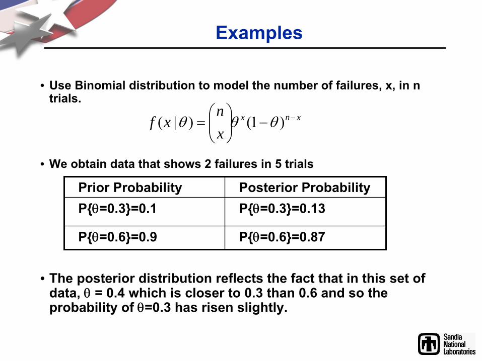
Examples

• Use Binomial distribution to model the number of failures, x, in

n trials.

• We obtain data that shows 2 failures in 5 trials

• The posterior distribution reflects the fact that in this set of

data, θ

= 0.4 which is closer to 0.3 than 0.6 and so the probability of θ=0.3 has risen slightly.

xnx

xn

xf −−⎟⎟⎠

⎞⎜⎜⎝

⎛= )1()|( θθθ

Prior Probability Posterior ProbabilityPθ=0.3=0.1 Pθ=0.3=0.13

Pθ=0.6=0.9 Pθ=0.6=0.87

Documents

From Uncertainty to Credibility: UQ Algorithms and …€¦ · · 2014-04-04(e.g., exhibits proper ... Sample Number Base 2 Base 3 Base 5 Base 7 1 0.5000 0.3333 0.2000 0.1429