Embed Size (px)
Citation preview
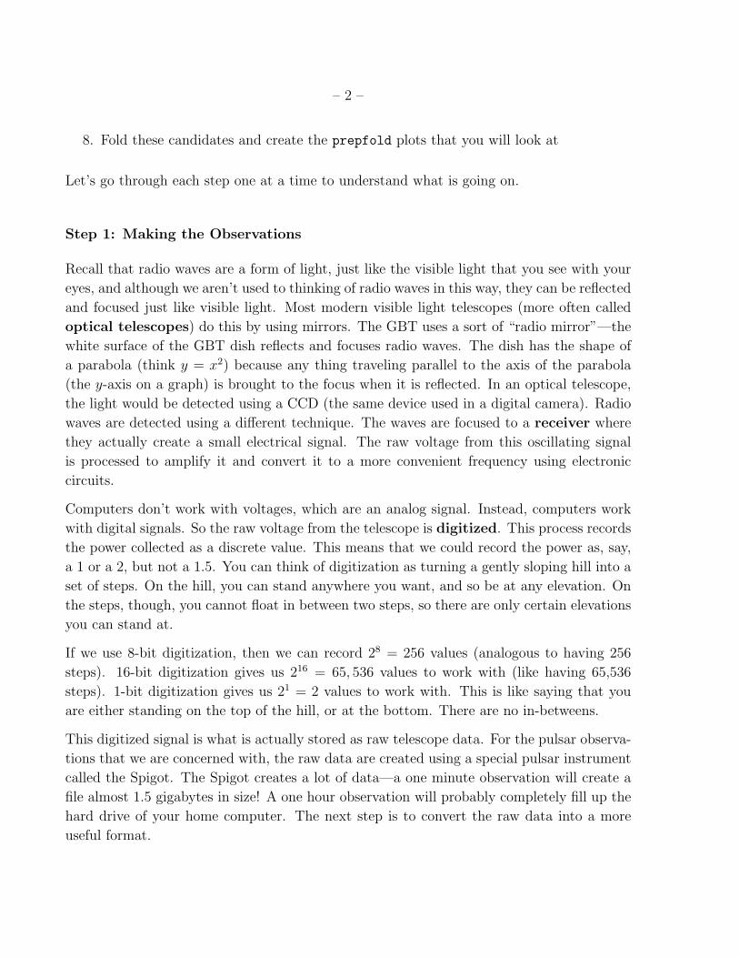
From the Telescope to the CollaboratoryProcessing GBT Data
Ryan Lynch
Department of Physics, McGill University
3600 University Street, Montreal, Quebec, H3A 2T8, Canada
Introduction
Your job in the Pulsar Search Collaboratory will be to analyze prepfold plots and determine
if they show evidence for a new pulsar. Searching for and Identifying Pulsars is a guide to
teach you how to do just that. However, it is also important to understand how the prepfold
plots are created, and how one makes them from data collected by the telescope, and that
is the purpose of this guide. With this information in hand you will be better able to
understand the information on a prepfold plot. Quite a bit goes on “under the hood” that
you might not otherwise be aware of, and each step is crucial when searching for new pulsars.
Throughout this guide I will reintroduce ideas covered in Searching for and Identifying Pul-
sars, so it would be good to read that first. However, for clarity I will reiterate and expand
on the necessary concepts from that guide. The idea is not to memorize every detail of the
data analysis, but rather to gain a broad sense of what is done. Having this global picture
will make you a better astronomer.
There are eight main steps that go into finding a new pulsar:
1. Make observations using the GBT and record the raw data
2. Convert these raw data into a more useful format that tells us the power collected by
the telescope
3. Search for RFI in the data and make sure that it is ignored during further analysis
4. De-disperse the data and convert it into a time series
5. Fourier transform the time series
6. Look for and remove RFI yet again
7. Search the Fourier spectrum for candidate pulsars
– 2 –
8. Fold these candidates and create the prepfold plots that you will look at
Let’s go through each step one at a time to understand what is going on.
Step 1: Making the Observations
Recall that radio waves are a form of light, just like the visible light that you see with your
eyes, and although we aren’t used to thinking of radio waves in this way, they can be reflected
and focused just like visible light. Most modern visible light telescopes (more often called
optical telescopes) do this by using mirrors. The GBT uses a sort of “radio mirror”—the
white surface of the GBT dish reflects and focuses radio waves. The dish has the shape of
a parabola (think y = x2) because any thing traveling parallel to the axis of the parabola
(the y-axis on a graph) is brought to the focus when it is reflected. In an optical telescope,
the light would be detected using a CCD (the same device used in a digital camera). Radio
waves are detected using a different technique. The waves are focused to a receiver where
they actually create a small electrical signal. The raw voltage from this oscillating signal
is processed to amplify it and convert it to a more convenient frequency using electronic
circuits.
Computers don’t work with voltages, which are an analog signal. Instead, computers work
with digital signals. So the raw voltage from the telescope is digitized. This process records
the power collected as a discrete value. This means that we could record the power as, say,
a 1 or a 2, but not a 1.5. You can think of digitization as turning a gently sloping hill into a
set of steps. On the hill, you can stand anywhere you want, and so be at any elevation. On
the steps, though, you cannot float in between two steps, so there are only certain elevations
you can stand at.
If we use 8-bit digitization, then we can record 28 = 256 values (analogous to having 256
steps). 16-bit digitization gives us 216 = 65, 536 values to work with (like having 65,536
steps). 1-bit digitization gives us 21 = 2 values to work with. This is like saying that you
are either standing on the top of the hill, or at the bottom. There are no in-betweens.
This digitized signal is what is actually stored as raw telescope data. For the pulsar observa-
tions that we are concerned with, the raw data are created using a special pulsar instrument
called the Spigot. The Spigot creates a lot of data—a one minute observation will create a
file almost 1.5 gigabytes in size! A one hour observation will probably completely fill up the
hard drive of your home computer. The next step is to convert the raw data into a more
useful format.
– 3 –
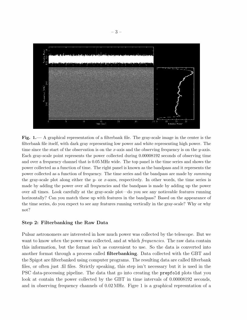
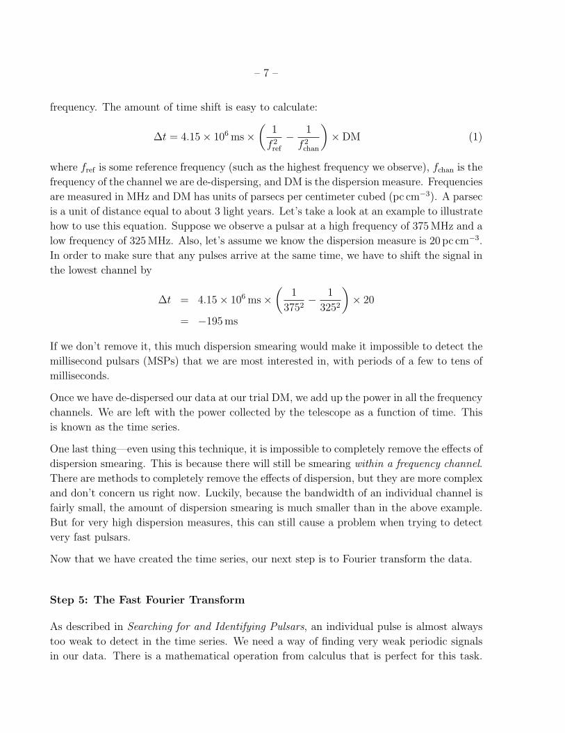
Fig. 1.— A graphical representation of a filterbank file. The gray-scale image in the center is the
filterbank file itself, with dark gray representing low power and white representing high power. The
time since the start of the observation is on the x-axis and the observing frequency is on the y-axis.
Each gray-scale point represents the power collected during 0.00008192 seconds of observing time
and over a frequency channel that is 0.05MHz wide. The top panel is the time series and shows the
power collected as a function of time. The right panel is known as the bandpass and it represents the
power collected as a function of frequency. The time series and the bandpass are made by summing
the gray-scale plot along either the y- or x-axes, respectively. In other words, the time series is
made by adding the power over all frequencies and the bandpass is made by adding up the power
over all times. Look carefully at the gray-scale plot—do you see any noticeable features running
horizontally? Can you match these up with features in the bandpass? Based on the appearance of
the time series, do you expect to see any features running vertically in the gray-scale? Why or why
not?
Step 2: Filterbanking the Raw Data
Pulsar astronomers are interested in how much power was collected by the telescope. But we
want to know when the power was collected, and at which frequencies. The raw data contain
this information, but the format isn’t as convenient to use. So the data is converted into
another format through a process called filterbanking. Data collected with the GBT and
the Spigot are filterbanked using computer programs. The resulting data are called filterbank
files, or often just .fil files. Strictly speaking, this step isn’t necessary but it is used in the
PSC data-processing pipeline. The data that go into creating the prepfold plots that you
look at contain the power collected by the GBT in time intervals of 0.00008192 seconds,
and in observing frequency channels of 0.02MHz. Figre 1 is a graphical represntation of a
– 4 –
filterbank file. Looking at it closely should help you to better understand the form of our
data.
Once the data have been filterbanked, we can proceed to the next step, which is finding and
removing RFI from our analysis.
Step 3: Finding RFI
Radio frequency interference, or RFI, can be a big problem for radio astronomers. Just like
optical astronomers can’t observe where there is too much light pollution, radio astronomers
need to go somewhere where the radio sky is “dark”. Because Green Bank is in the National
Radio Quiet Zone, there is usually very little RFI. But it is impossible to get rid of all sources
of RFI, so before we search our data for pulsars, we try identify as much of it as possible.
In Searching for and Identifying Pulsars we talked about how to recognize RFI in prepfold
plots, but it would be far too time consuming to look for all sources of RFI this way. Instead,
computer programs try to identify RFI automatically by looking at the statistics of the data.
The first step is to compute the average1 power of the data. We do this by de-dispersing at a
dispersion measure of zero and then adding up all of the individual frequency channels. We
will discuss de-dispersion in the next section, but for now all you need to know is that this
ensures that any signals we see in the data are coming from the Earth, and not space. The
result of the de-dispersion is a measure of power as a function of time. Once the average is
computed, we look for any time intervals that had a power level that was significantly higher
than the average. If this is the case, we remove those time intervals from further analysis.
This is known as clipping, because we essentially cut off any extremely high power levels.
In the previous step, we looked at the average value of the data over the course of the whole
observation and added up the power from all frequencies. In the next step we compute the
average for only small intervals of the data in both time and frequency. This step is best
illustrated with an example. Suppose that we calculate the average power of all frequency
channels for the first two seconds of our observation. We then compare this average to the
actual power in each individual frequency channel during that first two seconds. If the power
in a channel is much higher than the average, this channel is removed from analysis.
Next, we find the average of a single frequency channel during the whole course of our
observation. This might be the channel corresponding to a frequency of 350MHz. We then
1For those familiar with statistics, we calculate the median instead of the mean, because the median will
not be skewed as much by RFI.
– 5 –
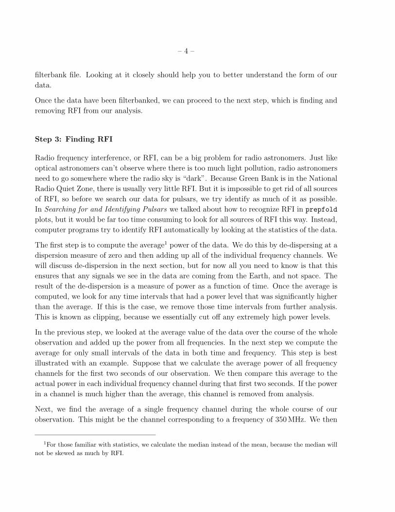
Fig. 2.— A graphical representation of an RFI mask. The observing frequency is on the x-axis
and the time since the start of the observation is on the y-axis. We typically split the observation
up into chunks about 2 seconds long, and these intervals are each given a number, which can be
seen on the right side. Any part of the data in black, red, green, or blue has been masked out.
The colors represent the specific problem with the data that caused it to be masked. Black means
that the user specified that the data be masked, or that a particular interval or frequency channel
was too contaminated. Red means that the total power in the part of the data was too high, green
means the data showed an abnormal standard deviation, and blue means the average of that data
was abnormally high.
look at each two second interval of the observation at that frequency. If the power in any
interval is significantly higher than the average, we remove it from analysis. We also remove
data if the standard deviation is abnormally high.
There is one last step to do. If a single time interval or frequency channel is very contaminated
with RFI, we will completely remove it from analysis, even if our program didn’t find RFI
in every frequency channel or every time interval. Typically, we remove anything more than
70% contaminated. The reasoning is that these intervals and channels probably are useless,
even if some of the RFI was just a little too weak to be identified.
When all is said and done, we are left with an RFI “mask”. This mask is used by other
programs to identify which time intervals and which frequency channels to ignore from
analysis. Figure 2 is a graphical representation of one such mask.
The next step is to de-disperse the data.
– 6 –
Step 4: De-dispersion
In order to find new pulsars, we must look for periodic signals in our data. A key to finding
the periodic signals is that they appear to be brief. If a pulsar beamed radio waves in our
direction during 100% of its rotation, it wouldn’t really look like a pulse. Instead, it would
look like a constant stream of power, like a light bulb that is left on. Because pulsar signals
are so weak, this wouldn’t seem very interesting—it would just appear as a slight increase
in the background level of radio waves. Luckily, pulsar pulses are only visible for a small
fraction of their rotation (typically a few percent). But there are effects that can cause the
duration of the pulses to appear longer. If these effects are severe, the narrow pulse can be
spread out too much to be detected. The principal culprit behind this broadening of the
pulse is called dispersion, and its effect is called dispersion smearing.
Dispersive smearing is caused by electrons in space. While space is very nearly empty, it isn’t
completely empty. One of the things that we find in space are electrons which aren’t bound
to any atom. These so-called free electrons can cause radio waves to slow down. How much
the radio waves slow down depends on their frequency, with lower frequencies being slowed
down more than higher frequencies. Since we observe pulsars over a range of frequencies,
typically 10s–100s of MHz, we are simultaneously collecting signal from the pulsar at both
lower and higher frequencies. Dispersion causes the low frequency pulsar signal to arrive at
Earth after the high frequency pulsar signal. If we were to naively add up the power at all
frequencies, the pulse would be spread out, possibly by too much to be detectable.
Luckily, we know how to remove the effects of dispersion if we know the dispersion mea-
sure, or DM. The dispersion measure is a way of describing how many electrons lie between
the pulsar and Earth. The more electrons there are, the higher the DM and hence the worse
the dispersion smearing. Consequently, a DM of zero tells us that the signal traveled through
no electrons on its way to Earth. But that is impossible for a real pulsar, which lies many
light years away and must ecnounter some electrons. The only explanation is that the signal
originated from the Earth; that is, the signal is actually RFI. This is useful because any
signals we see with a DM of zero must be RFI (see the above explanation of RFI removal).
The process of removing the effects of dispersion smearing is called de-dispersion.
But now we run into a conundrum. We have absolutely no way of knowing what a pulsar’s
dispersion measure will be without detecting the pulsar first, but we can’t detect the pulsar
unless we de-disperse at the appropriate DM! Our only option is to de-disperse at many
reasonable values of the dispersion measure. That is, we simply guess and see if any pulsars
show up.
The actual process of de-dispersion involves applying a time shift to the signal at some given
– 7 –
frequency. The amount of time shift is easy to calculate:
∆t = 4.15× 10⁶ ms×
(
1
f 2
ref
−
1
f 2
chan
)
×DM (1)
where fref is some reference frequency (such as the highest frequency we observe), fchan is the
frequency of the channel we are de-dispersing, and DM is the dispersion measure. Frequencies
are measured in MHz and DM has units of parsecs per centimeter cubed (pc cm−3). A parsec
is a unit of distance equal to about 3 light years. Let’s take a look at an example to illustrate
how to use this equation. Suppose we observe a pulsar at a high frequency of 375MHz and a
low frequency of 325MHz. Also, let’s assume we know the dispersion measure is 20 pc cm−3.
In order to make sure that any pulses arrive at the same time, we have to shift the signal in
the lowest channel by
∆t = 4.15× 10⁶ ms×
(
1
3752−
1
3252
)
× 20
= −195ms
If we don’t remove it, this much dispersion smearing would make it impossible to detect the
millisecond pulsars (MSPs) that we are most interested in, with periods of a few to tens of
milliseconds.
Once we have de-dispersed our data at our trial DM, we add up the power in all the frequency
channels. We are left with the power collected by the telescope as a function of time. This
is known as the time series.
One last thing—even using this technique, it is impossible to completely remove the effects of
dispersion smearing. This is because there will still be smearing within a frequency channel.
There are methods to completely remove the effects of dispersion, but they are more complex
and don’t concern us right now. Luckily, because the bandwidth of an individual channel is
fairly small, the amount of dispersion smearing is much smaller than in the above example.
But for very high dispersion measures, this can still cause a problem when trying to detect
very fast pulsars.
Now that we have created the time series, our next step is to Fourier transform the data.
Step 5: The Fast Fourier Transform
As described in Searching for and Identifying Pulsars, an individual pulse is almost always
too weak to detect in the time series. We need a way of finding very weak periodic signals
in our data. There is a mathematical operation from calculus that is perfect for this task.
– 8 –
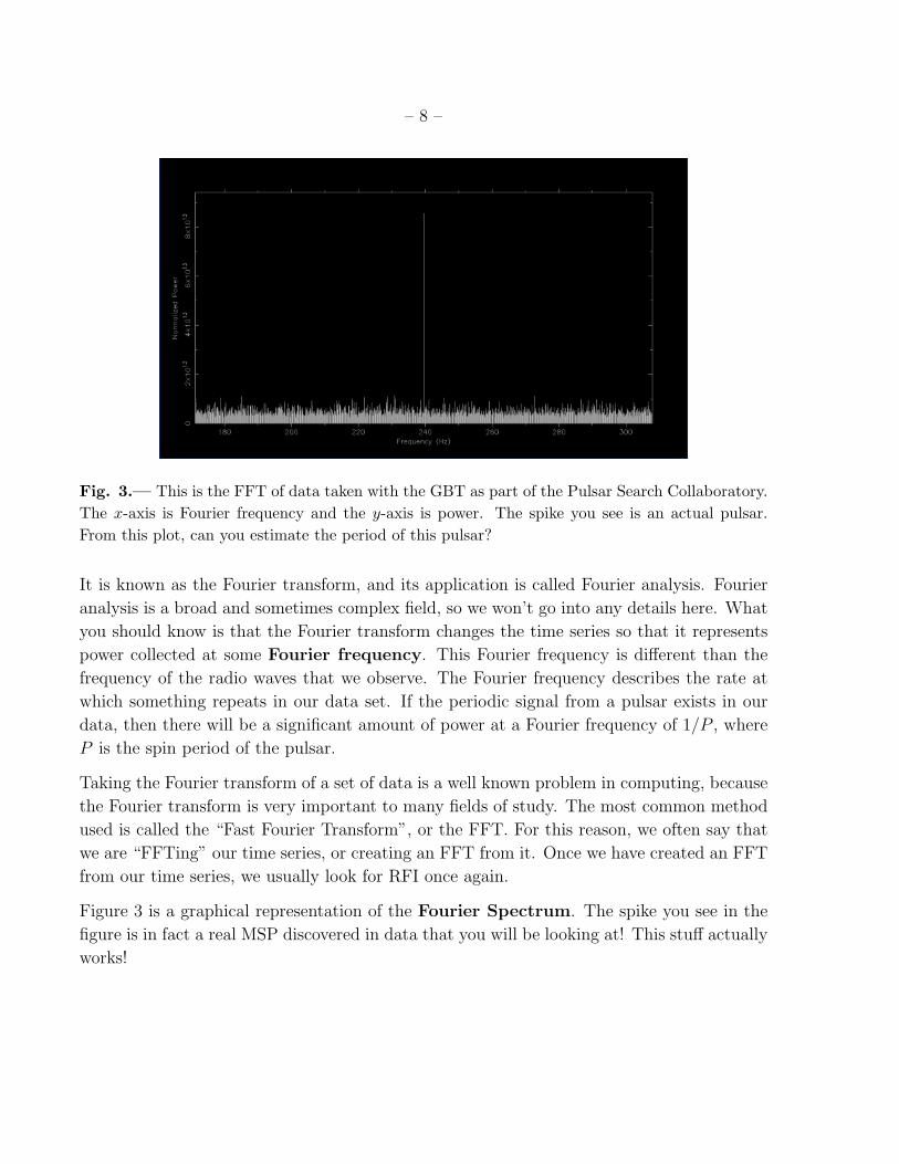
Fig. 3.— This is the FFT of data taken with the GBT as part of the Pulsar Search Collaboratory.
The x-axis is Fourier frequency and the y-axis is power. The spike you see is an actual pulsar.
From this plot, can you estimate the period of this pulsar?
It is known as the Fourier transform, and its application is called Fourier analysis. Fourier
analysis is a broad and sometimes complex field, so we won’t go into any details here. What
you should know is that the Fourier transform changes the time series so that it represents
power collected at some Fourier frequency. This Fourier frequency is different than the
frequency of the radio waves that we observe. The Fourier frequency describes the rate at
which something repeats in our data set. If the periodic signal from a pulsar exists in our
data, then there will be a significant amount of power at a Fourier frequency of 1/P , where
P is the spin period of the pulsar.
Taking the Fourier transform of a set of data is a well known problem in computing, because
the Fourier transform is very important to many fields of study. The most common method
used is called the “Fast Fourier Transform”, or the FFT. For this reason, we often say that
we are “FFTing” our time series, or creating an FFT from it. Once we have created an FFT
from our time series, we usually look for RFI once again.
Figure 3 is a graphical representation of the Fourier Spectrum. The spike you see in the
figure is in fact a real MSP discovered in data that you will be looking at! This stuff actually
works!
– 9 –
Step 6: Identifying RFI...Again
Although we have programs that can identify most sources of RFI, some will inevitably slip
through. For this reason, we usually create an FFT of a time series that has a dispersion
measure of zero. Recall that anything with a DM of zero must be man-made RFI. We can
then examine this FFT and look for strong signals. One very common signal that we see is
at a Fourier frequency of 60Hz. This corresponds to some source of radio waves that repeats
itself 60 times a second. Those of you familiar with electronics will know that this is exactly
the frequency of the alternating current that supplies power to our homes and businesses.
The RFI at 60Hz is therefore produced by the power lines that carry electricity. When we
see this type of signal in our FFT, we can explicitly ignore it during further analysis. In this
way we eliminate more potential sources of RFI.
Now that we have a removed RFI to the best of our ability, we are ready to search our data
for pulsars.
Step 7: Searching the Fourier Spectrum
Searching for pulsars is, in principle, a simple task. Once we de-disperse our data at some
trial DM and take the FFT, we simply need to search the Fourier spectrum for signals with
lots of power. If we find such a signal, we record information about it in a list of candidate
pulsars. Of course, since we don’t know the DM of the pulsars ahead of time, we must
try very many different dispersion measures. Furthermore, our FFTs are often very large,
containing millions of individual Fourier frequencies that need to be checked. Still, modern
computers are efficient at searching for pulsars. All that is needed is time.
There is one other effect that needs to be taken into account, though. Our description of
Fourier analysis so far has made an unspoken assumption that the period of the pulsar we
are trying to detect is constant throughout the observation. Imagine, though, that something
causes the pulsar to change period. At the beginning of the observation it might have a period
of 2.17436ms, and at the end it may have a period of 2.17440ms. During this time, the period
changes slowly between these two values. When we take the FFT of the time series, the
power will be spread out between the two Fourier frequency of 1/(2.17436ms) = 459.90Hz
and 1/(2.17440ms) = 459.89Hz. A pretty small change, to be sure, but enough to make it
difficult to detect such a pulsar. The reason is that a perfectly periodic signal (i.e., one with
a constant period), will usually have its power spread over a few thousandths of a Hz, and
often much less (the smallest component of Fourier frequency we can resolve is 1/T , where
T is the total observation time). A shift of even 0.01Hz is enough to spread the power out
– 10 –
so much that it is difficult to detect a pulsar unless it is very bright. It would be like taking
a very steep pile of dirt and spreading it out over a much larger area. Soon, you can’t even
tell that there was a pile there to begin with.
So what exactly would cause a pulsar’s period to change? Well, the rotation rate of all pulsars
is slowing down because the pulsar is simply losing energy. However, this is usually too small
an effect to be important for detecting pulsars. There is another, more important effect that
arises any time the pulsar is accelerating with respect to the telescope used to observe it.
This acceleration causes a Doppler shift, the same thing that causes an ambulance siren to
change in pitch when traveling towards or away from you. Suppose a pulsar is accelerating
away from our telescope. It sends out a pulse, which must travel through space. However,
when the next pulse is sent out, the pulsar is farther away. The pulse must travel a little
bit farther to reach the Earth, and the extra time it takes make it seem like the period is
longer than it actually is. If the pulsar is accelerating, then the time between the arrival of
successive pulses seems to get longer and longer, and the period seems to slow down. The
opposite happens if the pulsar is accelerating towards the Earth—the period seems to speed
up.
Because the Earth rotates around its axis and revolves around the Sun, there will always
be some acceleration between the telescope and the pulsar. We can remove this effect easily
because we can measure the motion of the Earth precisely. However, if the pulsar is orbiting
another star, then it too will accelerate. Other effects can cause acceleration as well. And it
just so happens that the pulsars that are most interesting, MSPs, are also the pulsars most
likely to have companion stars, and hence to be accelerating. So it is very important that
we find ways of detecting these accelerating pulsars. Of course, we don’t know what the
acceleration will be ahead of time. Just as we had to guess the DM when de-dispersing the
data, we also have to guess how much acceleration the pulsar is undergoing. Once we make
a guess, we can use detailed Fourier analysis to remove the effects of acceleration. But this
is another parameter we must search over, and another reason that finding pulsars requires
lots of computer power.
When all is said and done, though, we will have several candidates at several dispersion
measures and several amounts of acceleration. The next step is to examine the candidates
and decide which ones are real pulsars.
Step 8: The Human Touch
Everything we have discussed so far can be automated. A computer needs to only be
told what dispersion measures and accelerations to try, and it will take care of the rest.
– 11 –
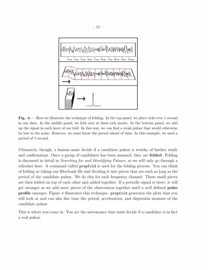
Fig. 4.— Here we illustrate the technique of folding. In the top panel, we place ticks ever 1 second
in our data. In the middle panel, we fold over at these tick marks. In the bottom panel, we add
up the signal in each layer of our fold. In this way, we can find a weak pulsar that would otherwise
be lost in the noise. However, we must know the period ahead of time. In this example, we used a
period of 1 second.
Ultimately, though, a human must decide if a candidate pulsar is worthy of further study
and confirmation. Once a group of candidates has been amassed, they are folded. Folding
is discussed in detail in Searching for and Identifying Pulsars, so we will only go through a
refresher here. A command called prepfold is used for the folding process. You can think
of folding as taking our filterbank file and dividing it into pieces that are each as long as the
period of the candidate pulsar. We do this for each frequency channel. These small pieces
are then folded on top of each other and added together. If a periodic signal is there, it will
get stronger as we add more pieces of the observation together until a well defined pulse
profile emerges. Figure 4 illustrates this technique. prepfold generates the plots that you
will look at and can also fine tune the period, acceleration, and dispersion measure of the
candidate pulsar.
This is where you come in. You are the astronomer that must decide if a candidate is in fact
a real pulsar.
– 12 –
Conclusion
I hope this guide has shed some light on how astronomers look for pulsars. The process is
complex, and I have done my best to simplify some of the the most difficult concepts. At
this point in your career, it is not important that you understand every aspect of finding
pulsars. Professional astronomers spend many years learning everything that they need to
implement all the steps that we have discussed. The Pulsar Search Collaboratory is designed
to expose you to some of these ideas. Hopefully your experiences will be the start of a life
long journey that takes you deeper into astronomy, and science in general.
Have fun!