Embed Size (px)
Citation preview
ptg
From the Library of Melissa Wong
ptg
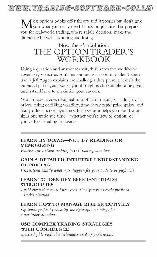
Most options books offer theory and strategies but don’t give you what you really need: hands-on practice that prepares
you for real-world trading, where subtle decisions make the difference between winning and losing.
Now, there’s a solution: THE OPTION TRADER’S
WORKBOOKUsing a question and answer format, this innovative workbook covers key scenarios you’ll encounter as an option trader. Expert trader Jeff Augen explains the challenges they present, reveals the potential pitfalls, and walks you through each example to help you understand how to maximize your success.
You’ll master trades designed to profit from rising or falling stock prices, rising or falling volatility, time decay, rapid price spikes, and many other market dynamics. Each section helps you build your skills one trade at a time—whether you’re new to options or you’ve been trading for years.
LEARN BY DOING—NOT BY READING ORMEMORIZINGPractice real decision-making in real trading situations
GAIN A DETAILED, INTUITIVE UNDERSTANDINGOF PRICINGUnderstand exactly what must happen for your trade to be profitable
LEARN TO IDENTIFY EFFICIENT TRADESTRUCTURESAvoid errors that cause losses even when you’ve correctly predicted a stock’s direction
LEARN HOW TO MANAGE RISK EFFECTIVELYOptimize profits by choosing the right option strategy for a particular situation
USE COMPLEX TRADING STRATEGIESWITH CONFIDENCEMaster highly profitable techniques used by professionals
From the Library of Melissa Wong

FFOORR SSAALLEE && EEXXCCHHAANNGGEE
wwwwww..ttrraaddiinngg--ssooffttwwaarree--ccoolllleeccttiioonn..ccoomm
MMiirrrroorrss::
wwwwww..ffoorreexx--wwaarreezz..ccoomm
wwwwww..ttrraaddeerrss--ssooffttwwaarree..ccoomm
wwwwww..ttrraaddiinngg--ssooffttwwaarree--ddoowwnnllooaadd..ccoomm
JJooiinn MMyy MMaaiilliinngg LLiisstt
ptg
THE
OPTIONTRADER’SW O R K B O O K
From the Library of Melissa Wong

ptg
This page intentionally left blank
From the Library of Melissa Wong
ptg
THE
OPTIONTRADER’SW O R K B O O KA PROBLEM-SOLVING APPROACH
JEFF AUGEN
From the Library of Melissa Wong
ptg
Vice President, Publisher: Tim MooreAssociate Publisher and Director of Marketing: Amy NeidlingerExecutive Editor: Jim BoydEditorial Assistants: Myesha Graham and Pamela BolandOperations Manager: Gina KanouseDigital Marketing Manager: Julie PhiferPublicity Manager: Laura CzajaAssistant Marketing Manager: Megan ColvinCover Designer: Chuti PrasertsithManaging Editor: Kristy HartProject Editor: Betsy HarrisCopy Editor: Cheri ClarkProofreader: Kathy RuizIndexer: WordWise Publishing Services LLCSenior Compositor: Gloria SchurickManufacturing Buyer: Dan Uhrig
© 2009 by Pearson Education, Inc.Publishing as FT PressUpper Saddle River, New Jersey 07458
This book is sold with the understanding that neither the author nor the publisher is engaged in renderinglegal, accounting or other professional services or advice by publishing this book. Each individual situationis unique. Thus, if legal or financial advice or other expert assistance is required in a specific situation, theservices of a competent professional should be sought to ensure that the situation has been evaluated care-fully and appropriately. The author and the publisher disclaim any liability, loss, or risk resulting directly orindirectly, from the use or application of any of the contents of this book.
FT Press offers excellent discounts on this book when ordered in quantity for bulk purchases or special sales. For moreinformation, please contact U.S. Corporate and Government Sales, 1-800-382-3419, [email protected] sales outside the U.S., please contact International Sales at [email protected].
Company and product names mentioned herein are the trademarks or registered trademarks of their respective owners.
All rights reserved. No part of this book may be reproduced, in any form or by any means, without permission in writingfrom the publisher.
Printed in the United States of America
First Printing December 2008
ISBN-10: 0-13-714810-0ISBN-13: 978-0-13-714810-3
Pearson Education LTD.Pearson Education Australia PTY, Limited.Pearson Education Singapore, Pte. Ltd.Pearson Education North Asia, Ltd.Pearson Education Canada, Ltd.Pearson Educación de Mexico, S.A. de C.V.Pearson Education—JapanPearson Education Malaysia, Pte. Ltd.
Library of Congress Cataloging-in-Publication Data
Augen, Jeffrey.
The option trader’s workbook : a problem-solving approach / Jeff Augen. — 1st ed.
p. cm.
Includes bibliographical references and index.
ISBN 0-13-714810-0 (pbk. : alk. paper) 1. Options (Finance) 2. Investment analysis. 3. Stock price forecasting.I. Title.
HG6024.A3A922 2008
332.63’2283—dc22
2008033614
From the Library of Melissa Wong

ptg
To Lisa and our little friends both past and present—
Spokes, Hobie, Einstein, Regis, Rocky, and Stella.
From the Library of Melissa Wong

ptg
This page intentionally left blank
From the Library of Melissa Wong
ptg
Contents
Preface . . . . . . . . . . . . . . . . . . . . . . . . . . . . .ix
Notes . . . . . . . . . . . . . . . . . . . . . . . . . . . . . . .1
Chapter 1 Pricing Basics . . . . . . . . . . . . . . . . . . . . . . . . .3Summary . . . . . . . . . . . . . . . . . . . . . . . . . . . . . . . . 42
Chapter 2 Purchasing Puts and Calls . . . . . . . . . . . . . .43Basic Dynamics (Problems #1–#7) . . . . . . . . . . . . 45Protecting Profit (Problems #8–#19) . . . . . . . . . . 49Defensive Action (Problems #20–#38). . . . . . . . . 59Term Structure, Volatility Skews, and Theta (Problems #39–#46) . . . . . . . . . . . . . . . . . . . . . . . 78Summary . . . . . . . . . . . . . . . . . . . . . . . . . . . . . . . . 90
Chapter 3 Covered Puts and Calls . . . . . . . . . . . . . . . .91Traditional Covered Positions Involving Stock and Options (Problems #1–#23) . . . . . . . . . . . . . . 93Pure Option Covered Positions (Problems #24–#28) . . . . . . . . . . . . . . . . . . . . . . 115Summary . . . . . . . . . . . . . . . . . . . . . . . . . . . . . . . 123
Chapter 4 Complex Trades—Part 1 . . . . . . . . . . . . . .125Vertical Spreads (Problems #1–#15). . . . . . . . . . 126Calendar Spreads (Problems #16–#30) . . . . . . . 136Diagonal Calendar Spreads Spanning Multiple Expirations and Strike Prices (Problems #31–#34) . . . . . . . . . . . . . . . . . . . . . . 154Ratio Trades (Problems #35–#41) . . . . . . . . . . . 163Summary . . . . . . . . . . . . . . . . . . . . . . . . . . . . . . . 172
From the Library of Melissa Wong
ptg
Chapter 5 Complex Trades—Part 2 . . . . . . . . . . . . . .173Butterfly Spreads (Problems #1–#8) . . . . . . . . . 174Straddles and Strangles (Problems #9–#16). . . . 185Four-Part Trades (Problems #17–#22) . . . . . . . . 194Volatility Index (Problems #23–#24) . . . . . . . . . 206Dividend Arbitrage (Problem #25). . . . . . . . . . . 211Summary . . . . . . . . . . . . . . . . . . . . . . . . . . . . . . . 214
Glossary . . . . . . . . . . . . . . . . . . . . . . . . . . .215
Index . . . . . . . . . . . . . . . . . . . . . . . . . . . . .221
viii THE OPTIONS TRADER’S WORKBOOK
From the Library of Melissa Wong
ptg
Preface
There are two kinds of successful investors: those who admit tooccasionally losing money and those who don’t. Despite claims to thecontrary, every investor loses money because risk always scales in pro-portion to reward. Long-term winners don’t succeed by never losing;they succeed because their trades are well thought out and carefullystructured. That said, very few investors recognize the impact of theirown trading mistakes.
These mistakes can be subtle. The classic example goes some-thing like this:
1. “I bought calls.”
2. “The stock went up, but I still lost money!”
This frustrating scenario in which an investor correctly predicts astock’s direction but loses money is incredibly common in the optiontrading world. Leverage is almost always the culprit. More precisely, itis the misuse of leverage that stems from a fundamental misunder-standing of risk that so often turns investing into gambling with thesimple click of a mouse. Option traders are famous for this mistake.They know, for example, that a sharp rise in the price of a stock cangenerate tremendous profit from nearly worthless far out-of-the-money calls. But lead is not so easily transmuted into gold. The prob-lem is entangled with complex issues like collapsing volatility,accelerating time decay, and regression toward the mean. Institu-tional traders understand these issues and they rarely make these mis-takes. Thousands of trades have taught them that not losing money isthe very best way to generate a profit.
It’s the thousands of trades, winners and losers both, that separateprofessionals from amateurs. Option trading is just like playing chess:It requires study and practice. The comparison is more valid than youmight think. Both chess and option trading are governed by a complexset of rules. Risk analysis is at the center of both games; so is posi-tional judgment and the ability to react quickly. Chess players learn toidentify patterns; option traders, in their own way, must learn to dothe same.
From the Library of Melissa Wong
ptg
This book is constructed around these themes. It is designed to letinvestors explore a vast array of rules and trade structures by solvingreal-life problems. This approach differs markedly from the catalog ofstructured trades that seems to have become the contemporary stan-dard for option trading books. Many fine texts have been written onthe subject, but most build on this design with slightly differentorganization or a few novel trading ideas. Collectively they miss thepoint. Learning to trade options is an active process, best accom-plished through doing rather than reading and memorizing. In thisregard we have avoided the familiar but bewildering list that includesnames like “reverse diagonal calendar spread,” “condor,” and “shortstrangle.” In their place you will find more descriptive phrases like“sell the near-dated option and buy the far-dated option.” But, moreimportantly, these descriptions appear in the context of trading situa-tions in which the reader is asked to make a choice, predict an out-come, or design a correction. Moreover, the problems build on eachother with each section progressing from basic to advanced.
Our goal was to challenge option traders at all levels. So take yourtime, work through the problems at a comfortable pace, and, mostimportant of all, make your trading mistakes here instead of in yourbrokerage account.
x THE OPTIONS TRADER’S WORKBOOK
From the Library of Melissa Wong

ptg
Acknowledgments
I would like to thank the team who helped pull the book together.First and foremost is Jim Boyd who was willing to take the risk of pub-lishing a new type of options book built around the problem-solvingconcept. His guidance and sound advice have added much clarity andorganization to the text. Authors create only rough drafts—finishedbooks are created by project editors. In that regard Betsy Harris wasresponsible for turning the original text into a publication-quality doc-ument. Without that effort the book would be nothing more than acollection of interesting math problems. I would also like to thankCheri Clark who carefully read and edited the text.
It is always difficult for an author to be objective about his ownwork. That job fell to Arthur Schwartz who patiently checked all mycalculations and made suggestions about new problems and examples.
Finally, I would like to acknowledge the excellent work of thePearson marketing team. I’ve certainly learned a great deal aboutweb-based digital marketing from working with Julie Phifer.
In these historic times of financial unrest, options have taken theirrightful place as sophisticated investment vehicles. Making themaccessible to a wider audience has been our principal goal.
From the Library of Melissa Wong
ptg
About the Author
Jeff Augen, currently a private investor and writer, has spentover a decade building a unique intellectual property portfolio ofdatabases, algorithms, and associated software for technical analysis ofderivatives prices. His work, which includes more than a million linesof computer code, is particularly focused on the identification of sub-tle anomalies and price distortions.
Augen has a 25 year history in information technology. As a co-founding executive of IBM’s Life Sciences Computing business, hedefined a growth strategy that resulted in $1.2 billion of new revenueand managed a large portfolio of venture capital investments. From2002 to 2005, Augen was President and CEO of TurboWorx Inc., atechnical computing software company founded by the chairman ofthe Department of Computer Science at Yale University. He is theauthor of two previous books: The Volatility Edge in Options Trading(FT Press 2008) and Bioinformatics in the Post-Genomic Era (Addi-son-Wesley 2005).
Much of his current work on option pricing is built around algo-rithms for predicting molecular structures that he developed manyyears ago as a graduate student in biochemistry.
From the Library of Melissa Wong
ptg
Notes
The following abbreviations will occasionally be used:
ATM = at-the-money (underlying security trades close to thestrike price)
OTM = out-of-the-money (underlying security trades belowthe strike price of a call or above the strike price of a put)
ITM = in-the-money (underlying security trades above thestrike price of a call or below the strike price of a put)
DITM = deep in-the-money (underlying security trades farabove the strike price of a call or far below the strike price of a put)
DOTM = deep out-of-the-money (underlying security tradesfar below the strike price of a call or far above the strike priceof a put)
Sqrt = Square root
StdDev = Standard deviations
1
From the Library of Melissa Wong

ptg
This page intentionally left blank
From the Library of Melissa Wong
ptg
Pricing Basics
The financial markets are a zero sum game where every dollarwon by one investor is lost by another. Knowledge and trading toolsare the differentiating factors that determine whether an investorlands on the winning or losing side. This book is designed to helpinvestors expand their knowledge of pricing and trading dynamics.The problems are designed to be solved using basic principles andsimple tools such as paper, pencil, and a calculator or spreadsheetprogram. Although you are strongly encouraged to become familiarwith the use of an option pricing calculator, that skill will not berequired to complete the problems in this book. However, it is alwaysadvantageous to explore different pricing scenarios with an optioncalculator and, in this context, you are encouraged to expand theproblems and concepts that appear throughout the book.
That said, such calculators are the most basic and essential toolfor an option trader. Their function is normally based on the Black-Scholes equations that describe the relationship between timeremaining in an option contract, implied volatility, the distancebetween the strike and stock prices, and short-term risk-free interestrates. Suitable versions are included in virtually every online tradingpackage offered by a broker in addition to dozens of examples thatcan be found on the web. For example, the Chicago Board OptionsExchange (CBOE) has an excellent set of educational tools thatincludes a fully functional options calculator. Readers are encouragedto visit this and other option trading sites and become familiar with
1
3
From the Library of Melissa Wong
ptg
such tools. More sophisticated calculators are available in the form ofposition modeling tools sold by a number of software vendors.
Many traders would argue that they don’t need to understandoption pricing theory because the markets are efficient, and options,if they are relatively liquid, are always fairly priced. That view isflawed—there are many reasons to understand pricing. Suppose, forexample, that you are faced with the choice of buying one of twoidentically priced call options that differ in strike price, volatility, andtime remaining before expiration. A logical choice can only be madeby a trader who understands the impact on price of each of thesecomponents. Structured positions composed of multiple options havemore complex dynamics that bring pricing theory even more sharplyinto focus. Moreover, implied volatility, a principal component in theprice of every option contract, varies considerably over time. It nor-mally rises in anticipation of an earnings announcement or otherplanned event and falls when the market is stable. Successful optiontraders spend much of their time studying these changes and usingthem to make informed decisions. Generally speaking, they try to sellvolatility that is overpriced and purchase options that are under-priced. Sophisticated institutional investors extend this approach byconstructing refined models called “volatility surfaces” that map avariety of parameters to a three-dimensional structure that can beused to predict options implied volatility. Custom surfaces can beconstructed for earnings season, rising and falling interest rate envi-ronments, bull or bear markets, strong or weak dollar environments,or any other set of conditions that affects volatility in a time or price-specific way. Regardless of the complexity of the approach, pricingtheory is always the foundation.
Options are enormously popular derivatives, and many strategy-specific subscription services have sprung up on the web. Thisapproach raises an important question: Is it better to choose a strat-egy and search for trade candidates, or to select stocks to trade and beflexible about the right strategy? Surprisingly, most option traders
4 THE OPTION TRADER’S WORKBOOK
From the Library of Melissa Wong
ptg
gain expertise trading a small number of position structures andsearch for candidates that fit. This search typically involves the use ofcharting software and a variety of tools for filtering stocks according toselectable criteria. Today’s online brokers compete for active tradersby continually upgrading the quality of their tools. Readers of thisbook are strongly encouraged to compare the offerings of differentbrokers to find those that best fit their needs. These tools combinedwith web-based services that provide historical stock and optionprices can be used to construct a comprehensive trading and analysisplatform.
Regardless of the approach—strategy or stock specific—pricing isthe core issue. Buying or selling options without thoroughly under-standing the subtle issues that impact their price throughout the expi-ration cycle is a mistake. We therefore begin with a chapter onpricing. Our approach is practical with a focus on trading. The con-cepts presented will form the basis for everything that is to follow,from basic put and call buying to complex multipart positions.
Unless otherwise stated, all examples for this chapter assume arisk-free interest rate of 3.5%.
1. A call option with a strike price of $100 trades for $3.00 with 14days remaining before expiration. What must the stock price beat expiration for the option to still be worth at least $3.00?
Answer: The stock price must be at or above $103 at expiration.
2. A put option with a strike price of $100 trades for $3.00 with 14days remaining before expiration. What must the stock price beat expiration for the option to still be worth at least $3.00?
Answer: The stock price must be at or below $97.
CHAPTER 1 • PRICING BASICS 5
From the Library of Melissa Wong
ptg
3. Suppose in each of the two examples described above, thestock was $15 out-of-the-money when the option traded for$3.00 with 14 days remaining. What can we conclude about thevolatility of the underlying stock?
Answer: The volatility must be very high for the option to bethis expensive with only 14 days remaining before expirationand the stock 15% out-of-the-money. (Actual implied volatilityis greater than 100% for each of these examples.)
4. A stock must continually move in the direction of the strikeprice to offset the effect of time decay. Assume the following:
Stock Price Call Price Days Remaining
$90 $2.22 100
$95 $2.22 50
Can you determine the strike price without knowing theimplied volatility or risk-free interest rate?
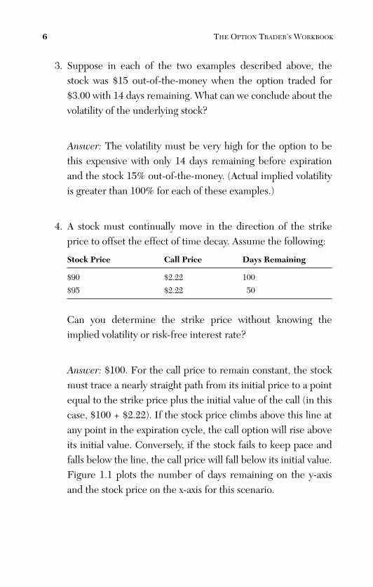
Answer: $100. For the call price to remain constant, the stockmust trace a nearly straight path from its initial price to a pointequal to the strike price plus the initial value of the call (in thiscase, $100 + $2.22). If the stock price climbs above this line atany point in the expiration cycle, the call option will rise aboveits initial value. Conversely, if the stock fails to keep pace andfalls below the line, the call price will fall below its initial value.Figure 1.1 plots the number of days remaining on the y-axisand the stock price on the x-axis for this scenario.
6 THE OPTION TRADER’S WORKBOOK
From the Library of Melissa Wong
ptg
Figure 1.1 Stock prices required to offset time decay in question #4.(Days remaining on the y-axis.)
5. Implied volatility for the call option in question #4 was 28.5%.In general terms, what would be the effect of doubling ortripling the implied volatility?
Answer: Increasing the volatility priced into the option contractwould raise the value of the midpoint ($95 with 50 daysremaining in problem #4), and endpoint ($102.22 at expirationin problem #4). The new initial option price would be muchhigher; the stock price would need to climb much faster; andthe expiration price would need to be much further in-the-money for the option to maintain its value. For example, in anextreme case where 200% implied volatility is priced into thesame option, the initial price with 100 days remaining would be$33.37. To sustain this option price with 50 days remaining, thestock would have to trade at $106.52. At expiration the stockwould need to trade $33.37 in-the-money—that is, the stockwould need to close the expiration cycle at a price of $133.37.
CHAPTER 1 • PRICING BASICS 7
0
20
40
60
80
100
$88 $90 $92 $94 $96 $98 $100 $102 $104
From the Library of Melissa Wong
ptg
6. Risk-free interest for the scenario in question #4 was 3.5%.What would be the effect of significantly increasing the rate ofrisk-free interest priced into the option contracts?
Answer: Raising the value of risk-free interest also increasesthe option price. As a result, the initial value with 100 daysremaining would be higher, the midpoint stock price thatwould have to be reached to maintain this price would behigher, and the stock would have to expire further into-the-money to maintain that price. However, the interest rate effectis much more subtle. If, for example, we used an extraordinaryrate ten times larger than that of the original scenario—that is,35%—then the table in question #4 would contain the values inthe following table:
Stock Price Call Price Days Remaining
$90.00 $4.96 100
$97.03 $4.96 50
The midpoint with 50 days remaining has climbed to $97.03,and the stock would need to climb to $104.96 at expiration forthe option to maintain its price. The subtle nature of the inter-est rate effect is apparent when one considers that this rela-tively small distortion required a hyperinflation value of 35%.However, the linear relationship between offsetting stock priceand time decay is preserved despite the extreme nature of theexample. As always, the stock price must follow a linear trajec-tory that ends at a point equal to the strike price plus the initialoption value for the call option price to remain constant.
8 THE OPTION TRADER’S WORKBOOK
From the Library of Melissa Wong
ptg
7. You might have noticed that the line displayed in the chartaccompanying question #4 is not perfectly straight. Can youexplain the subtle distortion?
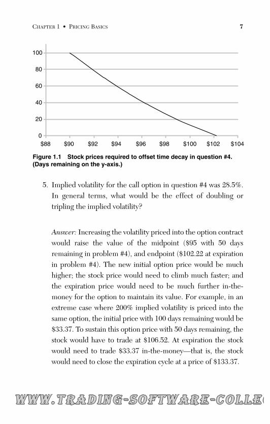
Answer: Time decay, also referred to as “theta,” accelerates asexpiration approaches. To maintain the option price, accelerat-ing time decay must be offset by larger moves of the underlyingstock. Some of the time decay acceleration is offset byincreased sensitivity of the option price to underlying stockmoves (delta rises as the stock approaches the strike price).However, the two forces do not exactly cancel. The differencegives rise to the subtle distortion and the line becomes a slightcurve. Accelerating time decay similarly affects puts and calls.Figure 1.2 displays the same curve for a put option with a $90strike price and the same implied volatility (28.5%). The con-stant price is $1.78. As before, the y-axis displays the number ofdays remaining and the x-axis the stock price.
CHAPTER 1 • PRICING BASICS 9
0
20
40
60
80
100
$86 $88 $90 $92 $94 $96 $98 $100 $102
Figure 1.2 Stock prices required to offset time decay for a $90 put with28.5% implied volatility. (Days remaining on the y-axis.)
From the Library of Melissa Wong
ptg
8. For a stock trading at $100, which option is more expensive—$105 call or $95 put? (Assume implied volatility, expirationdate, and so on, are all equal.)
Answer: $105 call. Option pricing models assign more value tothe call side. This asymmetry of price is related to the lognor-mal distribution that underlies all pricing calculations. In sim-ple terms, if a $100 stock loses 50% of its value twice, the stockwill trade at $25. However, if the same stock experiences two50% increases, it will rise $125 to $225. This effect causes callsto be more expensive than corresponding puts at the samestrike price. Thus, a sequence of price changes that generates a75% loss can be reversed to yield a 125% gain. These resultsimply that calls should be priced higher than puts at the samestrike price.
9. If XYZ is trading at $102.50 and the $100 strike price call isworth $3.00, would it be better to exercise or sell the option?
Answer: It rarely makes sense to exercise an option because allremaining time premium is lost. In this case we are told thatthe option is worth $3.00 but only $2.50 would be realized bycalling the stock (we would buy the stock for $100 and sell for$102.50). This dynamic holds until the final minutes of tradingwhen all premium disappears from the contracts. In practice,the final trade of an option contract usually lands in the handsof a broker who can exercise in-the-money contracts for verylittle cost.
10 THE OPTION TRADER’S WORKBOOK
From the Library of Melissa Wong
ptg
10. Suppose you are short the calls mentioned in problem #9 (stockis $2.50 in-the-money and calls are trading for $3.00). Howmuch money would be saved if the stock is called away fromyou?
Answer: 50¢.
11. Assume that it is expiration day and you are short at-the-moneycalls on a $100 stock—that is, the stock is trading right at thestrike price. What are the risks associated with letting theoption be exercised? If you already own the stock (coveredcalls), does it make sense to let it be called away?
Answer: All remaining time premium will disappear during thefinal few hours of trading. If, for example, the option is worth70¢ at the open and the stock remains at the strike price, theoption price will decline to just a few cents by the close. How-ever, the option price is very sensitive to changes that mightoccur in the underlying stock; this effect is enhanced as the dayprogresses and the option price approaches zero. Consider, forexample, how the stock price will affect the option price nearthe close when the option might be worth as little as a fewcents. Furthermore, the risk increases after the market closes ifthe stock trades in the after-hours session. The risk disappearsfor covered calls because the stock has already been purchased.Buying back inexpensive calls on the final day makes sensewhen it is undesirable to have the shares called away for otherreasons such as tax consequences or an expectation that theymight trade higher when the market reopens. With regard totrading costs, it is less expensive to allow the stock to be calledaway than to buy back short calls.
CHAPTER 1 • PRICING BASICS 11
From the Library of Melissa Wong
ptg
12. Delta represents the expected change in an option’s price for a1-point change in the underlying security. If a $3.00 call optionhas a delta of 0.35, what will the new option price be if thestock suddenly rises $1.00?
Answer: $3.35.
13. Suppose in question #12 the stock climbed $2.00. Would thenew option price be more or less than $3.70?
Answer: The new price will be higher because the call deltaincreases continuously as the stock rises. When the stock hasrisen $1.00, the new delta will be higher. Gamma is used todescribe the rate of change of delta.
14. Why is gamma always positive while delta is negative for putsand positive for calls?
Answer: Gamma represents the predicted change in delta for a1-point move in the underlying stock or index. When the stockprice rises, put and call deltas must both increase. The putdelta becomes less negative and the call delta becomes morepositive. In both cases gamma adds to the value of the delta.The opposite is true when a stock falls: The put delta becomesmore negative and the call delta becomes less positive.
12 THE OPTION TRADER’S WORKBOOK
From the Library of Melissa Wong
ptg
15. How is gamma affected by time and distance to the strikeprice? When does gamma have the highest value?
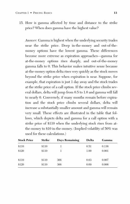
Answer: Gamma is highest when the underlying security tradesnear the strike price. Deep in-the-money and out-of-the-money options have the lowest gamma. These differencesbecome more extreme as expiration approaches—gamma forat-the-money options rises sharply, and out-of-the-moneygamma falls to 0. This behavior makes intuitive sense becauseat-the-money option delta rises very quickly as the stock movesbeyond the strike price when expiration is near. Suppose, forexample, that expiration is just 1 day away and the stock tradesat the strike price of a call option. If the stock price climbs sev-eral dollars, delta will jump from 0.5 to 1.0 and gamma will fallto nearly 0. Conversely, if many months remain before expira-tion and the stock price climbs several dollars, delta willincrease a substantially smaller amount and gamma will remainvery small. These effects are illustrated in the table that fol-lows, which depicts delta and gamma for a call option with astrike price of $110 when the underlying stock rises from at-the-money to $10 in-the-money. (Implied volatility of 50% wasused for these calculations.)
Stock Price Strike Days Remaining Delta Gamma
$110 $110 1 0.51 0.136
$120 $110 1 1.00 0.001
$110 $110 366 0.63 0.007
$120 $110 366 0.69 0.006
CHAPTER 1 • PRICING BASICS 13
From the Library of Melissa Wong
ptg
16. How is gamma affected by volatility?
Answer: Gamma falls as volatility rises for at-the-moneyoptions. Conversely, out-of-the-money options sometimesexperience rising gamma when volatility rises. Every stock andstrike price combination has a gamma peak at a specificimplied volatility.
17. How is delta affected by volatility? How does this behavior varywith time?
Answer: Near-dated, out-of-the-money options have substan-tial delta only if the underlying security is very volatile. At-the-money option delta is virtually unaffected by volatility changes,and delta falls sharply as volatility rises for in-the-moneyoptions. These effects make sense when they are recast in thecontext of risk management. A low volatility stock trading farfrom the strike price has little chance of ending up in-the-money; it has a characteristically low delta. Conversely, a highlyvolatile stock has a much greater chance of moving into-the-money and its delta is higher in proportion to this risk. Deep in-the-money call options have a small chance of falling below thestrike if the stock has low volatility. The delta on these optionswill be close to 1.0. If the same stock displayed very highvolatility, the price would have a reasonable chance of fallingbelow the strike and the calls would display a significantlylower delta.
These effects can be extended to explain the delta for optionsthat have many months left before expiration. Out-of-the-moneyoptions have higher deltas than their near-expiration counter-parts because they have much more time left to cross the strikeprice. Deep in-the-money long-dated call options have a lowerdelta than their near-expiration counterparts because they havemuch more time to fall below the strike price.
14 THE OPTION TRADER’S WORKBOOK
From the Library of Melissa Wong

FFOORR SSAALLEE && EEXXCCHHAANNGGEE
wwwwww..ttrraaddiinngg--ssooffttwwaarree--ccoolllleeccttiioonn..ccoomm
MMiirrrroorrss::
wwwwww..ffoorreexx--wwaarreezz..ccoomm
wwwwww..ttrraaddeerrss--ssooffttwwaarree..ccoomm
wwwwww..ttrraaddiinngg--ssooffttwwaarree--ddoowwnnllooaadd..ccoomm
JJooiinn MMyy MMaaiilliinngg LLiisstt
ptg
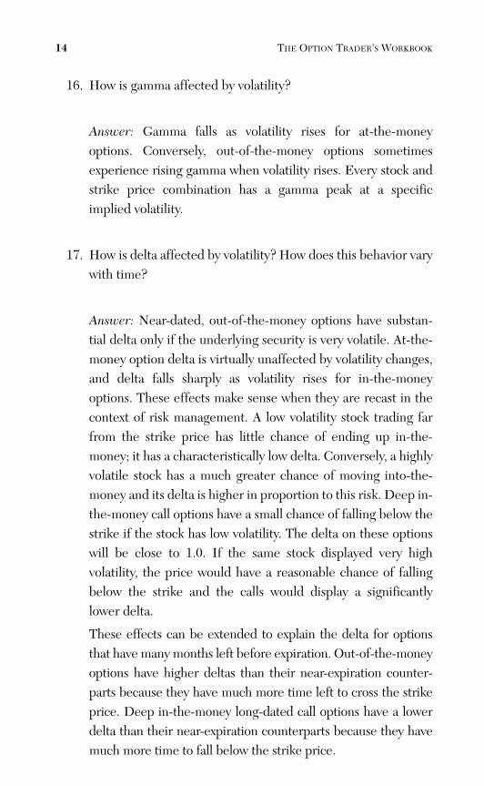
The following table summarizes this behavior. The left side dis-plays delta values for call options on two different stocks with18 days remaining before expiration, one with high volatilityand one with low volatility. The right side repeats these param-eters for calls that have one year left before expiration.
CHAPTER 1 • PRICING BASICS 15
365 Days Remaining/$110 Strike
Stock Price Volatility Delta
$100 0.20 0.42
$100 0.50 0.55
$110 0.20 0.61
$110 0.50 0.63
$120 0.20 0.76
$120 0.50 0.69
18 Days Remaining/$110 Strike
Stock Price Volatility Delta
$100 0.20 0.02
$100 0.50 0.22
$110 0.20 0.52
$110 0.50 0.53
$120 0.20 0.98
$120 0.50 0.80
18. Question #17 related delta to risk. How can the value of anoption delta be used as a guide for structuring a hedge?
Answer: The delta value is approximately equal to the chancethat an option will end up in-the-money. A call option with adelta of 0.35 should be expected to have a 35% chance of expir-ing in-the-money. At expiration, deep in-the-money calls have adelta of 1.0 and deep in-the-money puts have a delta of –1.0because each is almost guaranteed to expire in-the-money.These options behave like long and short stock respectively—that is, their prices change dollar-for-dollar with the stock price.
Stock hedges can be constructed to protect short positionsusing these parameters. To fully hedge 10 naked calls having adelta of 0.35, a short seller would need to purchase 350 sharesof the underlying security. The number of shares would need tovary as the stock rose and fell because the option delta wouldconstantly change. It would also need to change to accommo-date time decay and volatility swings in the underlying security.
From the Library of Melissa Wong
ptg
19. What would you expect the call option delta to be for a stockthat trades exactly at the strike price in the final few hoursbefore expiration?
Answer: 0.50 because there is approximately a 50% chance thatthe stock will close in-the-money.
20. For every straddle there is an underlying price point where thecall and put deltas are each exactly equal to 0.5. This parame-ter, known as the “delta neutral point,” depends on several fac-tors, including implied volatility, time remaining beforeexpiration, and price of the underlying stock or index. When isthe delta neutral point exactly equal to the strike price? Why isit not always equal to the strike price?
Answer: The delta neutral point of a straddle begins below thestrike price and rises at a constant rate until it equals the strikeprice at expiration. The same distortion that causes calls to bemore expensive than puts sets the delta neutral point below thestrike price (see question #8). Consequently, if a stock trades atthe strike price of a straddle prior to expiration, the price anddelta of the put will both be higher than those of the correspon-ding call.
21. Suppose with 300 days remaining before expiration, a put-calloption pair with a strike price of $100 is exactly delta neutralwith the stock trading at $87.66. When the new delta neutralpoint is $93.83, how many days will be left before expiration?At $96.92 how many days will be left?
16 THE OPTION TRADER’S WORKBOOK
From the Library of Melissa Wong
ptg
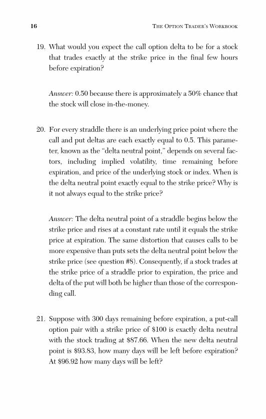
Answer: 150 days at $93.83 and 75 days at $96.92. The steadymovement of the delta neutral point is displayed in Figure 1.3.Days remaining before expiration are displayed on the y-axis,and the delta neutral stock price is displayed on the x-axis.
CHAPTER 1 • PRICING BASICS 17
0
50
100
150
200
250
300
350
$86 $88 $90 $92 $94 $96 $98 $100 $102
Figure 1.3 Migration of the delta neutral point for $100 strike pricestraddle beginning 300 days before expiration. Options for this examplewere priced with 50% implied volatility.
22. How would the slope of the line displayed in the answer toquestion #21 be affected if the implied volatility for both theput and the call were reduced by half?
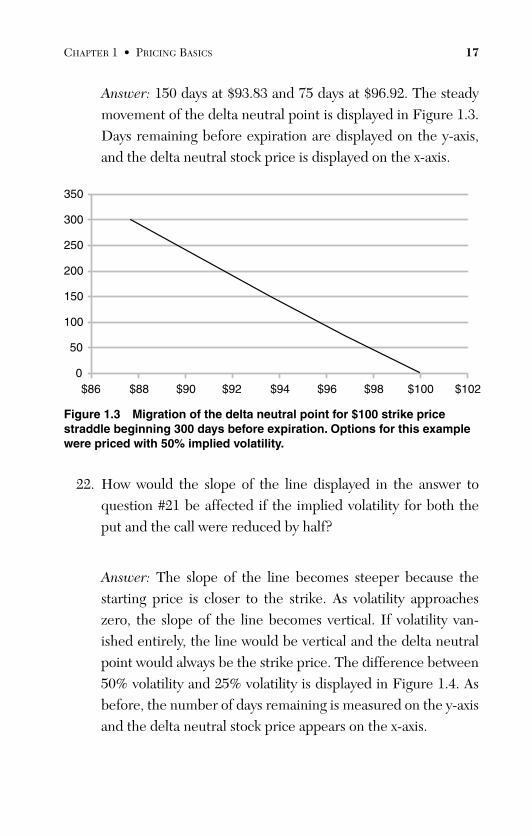
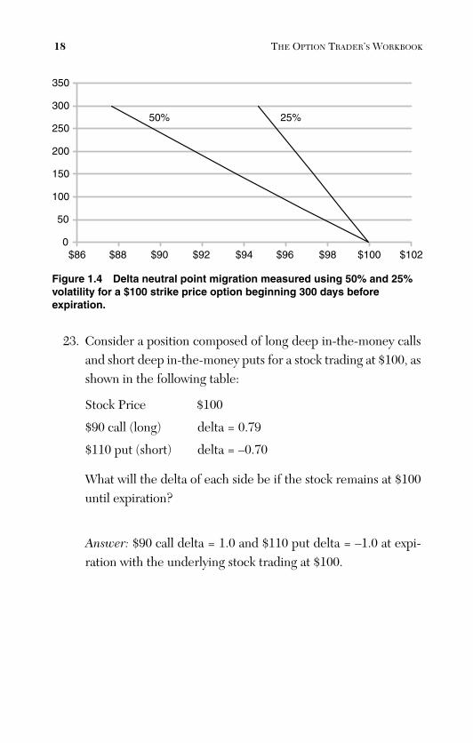
Answer: The slope of the line becomes steeper because thestarting price is closer to the strike. As volatility approacheszero, the slope of the line becomes vertical. If volatility van-ished entirely, the line would be vertical and the delta neutralpoint would always be the strike price. The difference between50% volatility and 25% volatility is displayed in Figure 1.4. Asbefore, the number of days remaining is measured on the y-axisand the delta neutral stock price appears on the x-axis.
From the Library of Melissa Wong
ptg
Figure 1.4 Delta neutral point migration measured using 50% and 25%volatility for a $100 strike price option beginning 300 days before expiration.
23. Consider a position composed of long deep in-the-money callsand short deep in-the-money puts for a stock trading at $100, asshown in the following table:
Stock Price $100
$90 call (long) delta = 0.79
$110 put (short) delta = –0.70
What will the delta of each side be if the stock remains at $100until expiration?
Answer: $90 call delta = 1.0 and $110 put delta = –1.0 at expi-ration with the underlying stock trading at $100.
18 THE OPTION TRADER’S WORKBOOK
0
50
100
150
200
250
300
350
$86 $88
50% 25%
$90 $92 $94 $96 $98 $100 $102
From the Library of Melissa Wong
ptg
24. Suppose that in question #23 the $90 call originally cost $12.30and the $110 put sold for $12.05—that is, the total position hada net cost of only 25¢. What was the final gain or loss?
Answer: At expiration the call and put were each worth $10.00,so the final position was long $10.00 (call) and short $10.00(put) with a net value of $0.00. Therefore, the trade lost $0.25.
25. Assume that the trade in questions #23 and #24 was long 10 callsand short 10 puts. Can you calculate the collateral requirementfor the trade? What was the total cost of owning the position?1
Answer: It is necessary to set aside 20% of the value of theunderlying stock for the short side of the trade. Since we sold10 put contracts for a $100 stock, the cost would be 0.20 × $100per share × 10 contracts × 100 shares per contract = $20,000.We must add the value realized from the sale of the put($12,050 + $20,000 = $32,050).
On the long side we would need to have enough cash on handto purchase the calls = $12.30 × 10 contracts × 100 shares percontract = $12,300. Therefore, the account must have $44,350to execute the initial trade. At expiration $0.25 was lost = $0.25× 10 contracts × 100 shares per contract = $250. The total costof holding the trade was $250 plus opportunity cost on $44,350during the lifetime of the trade.
CHAPTER 1 • PRICING BASICS 19
1 Collateral and margin requirements for option traders can vary by broker. Fur-thermore, recent changes allow customers whose accounts exceed certain mini-mum thresholds to take advantage of portfolio margining rules which moreprecisely align collateral requirements with overall portfolio risk. Readers wish-ing to further explore margin and collateral requirements are encouraged to visitthe Chicago Board Options Exchange website and to contact their broker.
From the Library of Melissa Wong
ptg
26. Consider a position composed of long out-of-the-money callsand long out-of-the-money puts for a stock trading at $100, asshown in the following table:
Stock Price $100
$110 call (long) delta = 0.30
$90 put (long) delta = –0.21
What will the delta of each side be if the stock remains at $100until expiration? What will the options be worth?
Answer: $110 call delta = 0 and $90 put delta = 0 at expirationwith the underlying stock trading at $100. Both options lose alltheir value.
27. Over what range of stock prices will the loss at expiration be100%?
Answer: Both options will expire worthless with the stockbetween $90 and $110. The total range for a return of $0.00 is$20.00. Outside this range, one of the options will have somevalue.
28. Assume that the calls in question #26 cost $2.56 and the putscost $1.86. At expiration, what underlying stock prices arebreak-even points for the trade? Is any collateral required forthis position?
Answer: The total cost was $4.42. Break-even points are$114.42 on the upside and $85.58 on the downside. These val-ues are determined by adding $4.42 to the $110 call strike andsubtracting $4.42 from the $90 put strike. No collateral was
20 THE OPTION TRADER’S WORKBOOK
From the Library of Melissa Wong
ptg
required because both sides were long. The trade would haveoriginally cost $442 for each pair of contracts.
29. Assume that the trade originally described in question #26decays to $0.00 with the stock at $100 and 1 day left beforeexpiration. An unsubstantiated rumor surfaces that the stock inquestion might be acquired, and implied volatility soars to veryhigh levels. Is there a level of implied volatility that couldrestore the price of each option to its original value despitebeing $10 out-of-the-money with only 1 day left? Would putand call deltas also be restored?
Answer: Yes, as long as there is time left in the contracts, it ispossible for volatility to rise high enough to restore the originalprices and deltas. If, for example, the original implied volatilitywas 40% and 50 days remained before expiration, a newimplied volatility around 280% would restore the original val-ues. Option prices on both sides of the trade would regain theiroriginal sensitivity to underlying price changes. However,because the delta-neutral point of the position would haveshifted slightly over the 50 days that the trade was open, thenew call price would be a few cents lower and the put price afew cents higher to achieve the same overall position value.These distortions are very slight for options that are 10% out-of-the-money. Actual values are listed in the following table.
DaysRemaining Put ($) Call ($) Volatility Delta
50 1.86 0.40 –0.21
50 2.56 0.40 0.30
1 1.98 2.78 –0.22
1 2.45 2.78 0.29
CHAPTER 1 • PRICING BASICS 21
From the Library of Melissa Wong
ptg
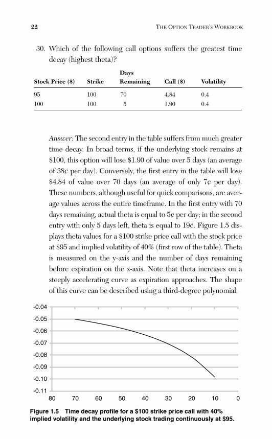
30. Which of the following call options suffers the greatest timedecay (highest theta)?
DaysStock Price ($) Strike Remaining Call ($) Volatility
95 100 70 4.84 0.4
100 100 5 1.90 0.4
Answer: The second entry in the table suffers from much greatertime decay. In broad terms, if the underlying stock remains at$100, this option will lose $1.90 of value over 5 days (an averageof 38¢ per day). Conversely, the first entry in the table will lose$4.84 of value over 70 days (an average of only 7¢ per day).These numbers, although useful for quick comparisons, are aver-age values across the entire timeframe. In the first entry with 70days remaining, actual theta is equal to 5¢ per day; in the secondentry with only 5 days left, theta is equal to 19¢. Figure 1.5 dis-plays theta values for a $100 strike price call with the stock priceat $95 and implied volatility of 40% (first row of the table). Thetais measured on the y-axis and the number of days remainingbefore expiration on the x-axis. Note that theta increases on asteeply accelerating curve as expiration approaches. The shapeof this curve can be described using a third-degree polynomial.
22 THE OPTION TRADER’S WORKBOOK
-0.11
-0.10
-0.09
-0.08
-0.07
-0.06
-0.05
-0.04
01020304050607080
Figure 1.5 Time decay profile for a $100 strike price call with 40%implied volatility and the underlying stock trading continuously at $95.
From the Library of Melissa Wong
ptg
31. Given the trading price of a call option, can the fair value of aput at the same strike price be determined? What informationis needed?
Answer: Yes—the put price can be calculated using the formulafor put-call parity. This formula is derived from the Black-Scholes equations that are used to price puts and calls. Fornon-dividend-paying stocks:
C + Xe-rt = P + S0
C = call price X = strike price
P = put price t = time remaining as
r = risk-free interest rate % of a year
S0 = stock price e = base of the naturallogarithm (2.718)
32. Suppose you were to discover a mispriced set of options forwhich the call was relatively more expensive than the put. Isthere a way to exploit this situation?
Answer: Put-call parity violations create arbitrage opportuni-ties that normally disappear very quickly. Bid-ask spreads andtrading costs make it nearly impossible for a public customer toexploit the arbitrage. Furthermore, the correct method fortrading such an arbitrage is complex. It involves selling theoverpriced calls, purchasing puts, and balancing the positionwith a stock-bond portfolio composed of long stock and shortbonds. The trade is unwound at expiration for a small profit. Inessence we would be long the right side of the equation andshort the overpriced left side.
CHAPTER 1 • PRICING BASICS 23
From the Library of Melissa Wong
ptg
24 THE OPTION TRADER’S WORKBOOK
33. What is the primary difference between European- and Ameri-can-style options?
Answer: European options can be exercised only at expiration.American-style options can be exercised at any time. Indexoptions are often European and equity options are almostinvariably American. Option pricing models are designedaround the European expiration and it is always assumed thatthe option will be bought and sold but not exercised beforeexpiration.
34. Suppose an investor is long calls on an index with Europeanexpiration rules. Can you envision issues related to the Euro-pean-style expiration that could affect liquidity or bid-askspreads?
Answer: When investors anticipate that a sudden large move willbe short-lived, bid-ask spreads and liquidity issues can surface,making it difficult to close an option position. This problem iswell-known to investors who trade options on the CBOE Volatil-ity Index (VIX). The VIX tends to rise sharply in a marketdecline and fall when the market stabilizes. In principle out-of-the-money calls should gain in value during a market drawdown.However, the anticipation of a sharp decline in the index as themarket regains stability after a sudden drop can create price dis-tortions for options that cannot be exercised. Consider, forexample, the thought process of an investor who is short callsthat suddenly move in-the-money as the index rises during amarket crash. Knowing that the VIX is likely to decline as themarket stabilizes, and that implied volatilities of VIX options willultimately fall, the investor will likely hesitate before closing theposition at a loss. This approach could not be taken if the calls
From the Library of Melissa Wong
ptg
were immediately exercisable. Unfortunately, because they arenot, bid-ask spreads tend to widen by a surprising amount andliquidity becomes an issue. These factors ultimately limit thevalue of out-of-the-money VIX calls as a hedge against a marketcrash. Some of the same effect can be seen with thinly tradedequity options. Holders of long puts often find it difficult to selltheir options for a fair price during a rapid market declinebecause short sellers of the same puts are unwilling to overpayto buy them back until volatility stabilizes. However, unlikeEuropean options that cannot be exercised before expiration,American options can never be worth less than the amount thatthey are in-the-money. This fact limits the size of the distortion.
35. What is the value of a 1 standard deviation daily price changefor a $100 stock having 30% implied volatility? What would bethe value of a 1 standard deviation monthly change for thesame stock?
Answer: Annual volatility is equal to the expected 1 year, 1 stan-dard deviation price change. Because volatility is proportionalto the square root of time, we can derive the value for a shortertimeframe by dividing the annual value by the square root ofthe number of shorter timeframes contained in 1 year. To cal-culate monthly volatility we would divide annual volatility bythe square root of 12; weekly volatility would be equal toannual volatility divided by the square root of 52. There is somedisagreement about the adjustment factor for daily volatilitybecause a calendar year contains approximately 252 tradingdays. Using this number we would divide by 15.87 to obtaindaily volatility which is also equal to the value of a close-to-close 1 standard deviation price change.
CHAPTER 1 • PRICING BASICS 25
From the Library of Melissa Wong
ptg
Assuming 252 trading days per year, the value of a daily 1 stan-dard deviation price change for a $100 stock with 30% impliedvolatility would be $100 × 0.30 / Sqrt (252) = $1.89.
The value of a 1 month, 1 standard deviation change would begiven by $100 × 0.30 / Sqrt(12) = $8.66.
In each case, multiplying by the annualization factor wouldreturn the value of a 1 year, 1 standard deviation price change.
$1.89 × Sqrt(252) = $30
$8.66 × Sqrt(12) = $30
36. For the stock in question #35, what is the probability that thestock will trade between $70 and $130 at the end of 1 year?
Answer: According to the normal distribution, the chance thatthe stock will trade in an interval that is bounded by 1 standarddeviation above and below the current price is approximately68%. Extending this calculation to the 1 day, 1 standard devia-tion change of question #35 sets the probability that the stockwill rise or fall less than $1.89 in a single day at 68%.
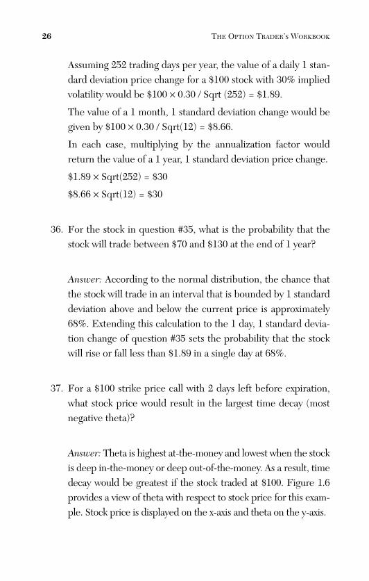
37. For a $100 strike price call with 2 days left before expiration,what stock price would result in the largest time decay (mostnegative theta)?
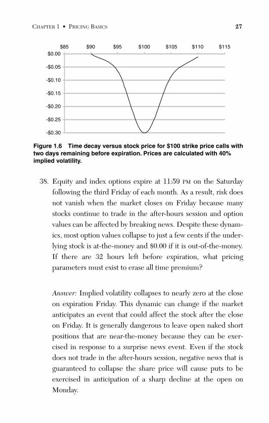
Answer: Theta is highest at-the-money and lowest when the stockis deep in-the-money or deep out-of-the-money. As a result, timedecay would be greatest if the stock traded at $100. Figure 1.6provides a view of theta with respect to stock price for this exam-ple. Stock price is displayed on the x-axis and theta on the y-axis.
26 THE OPTION TRADER’S WORKBOOK
From the Library of Melissa Wong
ptg
Figure 1.6 Time decay versus stock price for $100 strike price calls withtwo days remaining before expiration. Prices are calculated with 40%implied volatility.
38. Equity and index options expire at 11:59 PM on the Saturdayfollowing the third Friday of each month. As a result, risk doesnot vanish when the market closes on Friday because manystocks continue to trade in the after-hours session and optionvalues can be affected by breaking news. Despite these dynam-ics, most option values collapse to just a few cents if the under-lying stock is at-the-money and $0.00 if it is out-of-the-money.If there are 32 hours left before expiration, what pricingparameters must exist to erase all time premium?
Answer: Implied volatility collapses to nearly zero at the closeon expiration Friday. This dynamic can change if the marketanticipates an event that could affect the stock after the closeon Friday. It is generally dangerous to leave open naked shortpositions that are near-the-money because they can be exer-cised in response to a surprise news event. Even if the stockdoes not trade in the after-hours session, negative news that isguaranteed to collapse the share price will cause puts to beexercised in anticipation of a sharp decline at the open on Monday.
CHAPTER 1 • PRICING BASICS 27
-$0.30
-$0.25
-$0.20
-$0.15
-$0.10
-$0.05
$0.00$85 $90 $95 $100 $105 $110 $115
From the Library of Melissa Wong
ptg
39. Is it possible for the price of a call to rise or remain the samewhen the underlying stock or index falls?
Answer: Yes, because volatility tends to rise when prices fall. Inthe event of very damaging news, a stock can plunge andvolatility can rise sharply. For example, consider the followingscenario:
Acme stock trading at $100 and $105 strike price calls pricedwith 30% implied volatility and 90 days remaining before expi-ration are worth $4.23. Just after the market opens, Acmereports disappointing earnings and the stock falls 25%, withoptions implied volatility rising sharply to 120%. Put-call paritywill raise implied volatility for the calls in concert with the puts.Despite the 25% drop in stock price, $105 strike price calls willrise from $4.23 to $9.41. The stock would need to fall below$60—a 40% loss—to offset this rise in volatility. The followingtable summarizes this behavior.
DaysStock ($) Call ($) Volatility Strike ($) Remaining
100 4.23 0.30 105 90
75 9.41 1.20 105 90
60 4.40 1.20 105 90
This scenario played out in early 2008 when large investmentbanks suffered billions of dollars in “write downs” during acredit crisis precipitated by subprime lending. For example,call options on Bear Stearns stock that previously traded withimplied volatility in the 25% range spiked to more than 120%in early March. While the stock declined more than 35% dur-ing 10 trading sessions, rising volatility often caused call pricesto also rise. The effect was most prominent on March 14 whenthe stock suddenly plunged 48% in the first 30 minutes of trad-ing, and implied volatility skyrocketed to more than 450% forat-the-money calls.
28 THE OPTION TRADER’S WORKBOOK
From the Library of Melissa Wong
ptg
Modest changes in volatility can have similar effects. In our exam-ple, if Acme stock fell $8.00 and volatility climbed from 30% to50%, call prices would increase slightly despite the 8% underlyingprice decline. Details are outlined in the following table.
Stock ($) Call ($) Volatility Strike ($) Days Remaining
100 4.23 0.30 105 90
92 4.81 0.50 105 90
40. With regard to question #39, can you think of a reverse scenarioin which the stock price falls rapidly and puts also lose value?
Answer: When an uncertain situation resolves itself, volatilitycan fall rapidly. This effect is often tied to earnings releases.For stocks that have a history of large earnings-associated pricespikes, the market tends to overprice options by setting impliedvolatility inappropriately high prior to the event. The distortionis especially large when an earnings release coincides withoptions expiration. For these stocks, implied volatility risessharply to offset the rapid time decay of the final few days ofthe expiration cycle. Implied volatility normally returns to nor-mal levels immediately after earnings are announced. Even ifthe stock price declines sharply, collapsing volatility can reducethe value of put options. This effect is most pronounced forout-of-the-money puts. The following table outlines a simpleexample of a stock trading at $105 and $100 strike price putswith 15 days remaining before expiration. Despite a $5.00underlying price decline, out-of-the-money put values fallmore than 45% as volatility shrinks from 80% to 30%. Had theevent occurred in the final few days of the expiration cycle, theinitial volatility would have been much higher and the collapsewould have been much more pronounced.
CHAPTER 1 • PRICING BASICS 29
From the Library of Melissa Wong
ptg
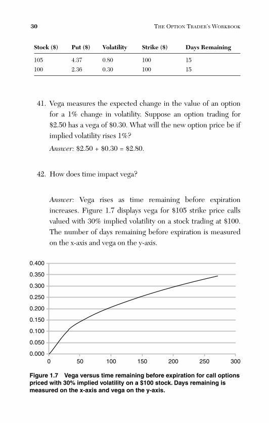
Stock ($) Put ($) Volatility Strike ($) Days Remaining
105 4.37 0.80 100 15
100 2.36 0.30 100 15
41. Vega measures the expected change in the value of an optionfor a 1% change in volatility. Suppose an option trading for$2.50 has a vega of $0.30. What will the new option price be ifimplied volatility rises 1%?
Answer: $2.50 + $0.30 = $2.80.
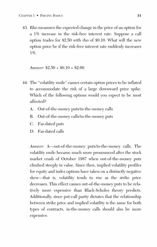
42. How does time impact vega?
Answer: Vega rises as time remaining before expirationincreases. Figure 1.7 displays vega for $105 strike price callsvalued with 30% implied volatility on a stock trading at $100.The number of days remaining before expiration is measuredon the x-axis and vega on the y-axis.
30 THE OPTION TRADER’S WORKBOOK
0.000
0.050
0.100
0.150
0.200
0.250
0.300
0.350
0.400
0 50 100 150 200 250 300
Figure 1.7 Vega versus time remaining before expiration for call optionspriced with 30% implied volatility on a $100 stock. Days remaining ismeasured on the x-axis and vega on the y-axis.
From the Library of Melissa Wong
ptg
43. Rho measures the expected change in the price of an option fora 1% increase in the risk-free interest rate. Suppose a calloption trades for $2.50 with rho of $0.10. What will the newoption price be if the risk-free interest rate suddenly increases1%.
Answer: $2.50 + $0.10 = $2.60.
44. The “volatility smile” causes certain option prices to be inflatedto accommodate the risk of a large downward price spike.Which of the following options would you expect to be mostaffected?
A. Out-of-the-money puts/in-the-money calls
B. Out-of-the-money calls/in-the-money puts
C. Far-dated puts
D. Far-dated calls
Answer: A—out-of-the-money puts/in-the-money calls. Thevolatility smile became much more pronounced after the stockmarket crash of October 1987 when out-of-the-money putsclimbed steeply in value. Since then, implied volatility profilesfor equity and index options have taken on a distinctly negativeskew—that is, volatility tends to rise as the strike pricedecreases. This effect causes out-of-the-money puts to be rela-tively more expensive than Black-Scholes theory predicts.Additionally, since put-call parity dictates that the relationshipbetween strike price and implied volatility is the same for bothtypes of contracts, in-the-money calls should also be moreexpensive.
CHAPTER 1 • PRICING BASICS 31
From the Library of Melissa Wong
ptg
45. Option traders often substitute deep-in-the-money calls forstock because the delta is close to 1.0 and the option pricechanges point-for-point with the stock price. Suppose we pur-chase 10 contracts of a $50 strike price call with a delta of 1.0on a stock that trades for $75. If the stock were to fall $20,which of the following would be true?
A. The option trade would lose more value than 1,000 sharesof stock.
B. The option trade would lose less value than 1,000 shares ofstock.
C. Both trades would lose $20,000.
Answer: B—The option trade would lose less than the equiva-lent stock trade. The equivalent stock trade consisting of 1,000shares would lose $20,000 because the delta of stock is alwaysexactly 1.0. However, the call option delta would shrink as theprice falls. In this case a $20 decrease in the stock price wouldresult in the call option being only $5.00 in-the-money. For a$50 strike price call with 90 days left before expiration andimplied volatility of 30%, the delta would fall to around 78%.The actual change in value for this trade would be $18,890.
Additional comments regarding the volatility smile:
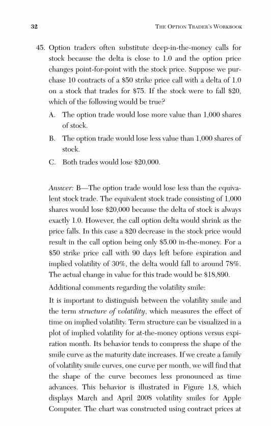
It is important to distinguish between the volatility smile andthe term structure of volatility, which measures the effect oftime on implied volatility. Term structure can be visualized in aplot of implied volatility for at-the-money options versus expi-ration month. Its behavior tends to compress the shape of thesmile curve as the maturity date increases. If we create a familyof volatility smile curves, one curve per month, we will find thatthe shape of the curve becomes less pronounced as timeadvances. This behavior is illustrated in Figure 1.8, which displays March and April 2008 volatility smiles for Apple Computer. The chart was constructed using contract prices at
32 THE OPTION TRADER’S WORKBOOK
From the Library of Melissa Wong
ptg
the market close on March 14 (AAPL trading at $127). Volatil-ity is measured on the y-axis and strike price on the x-axis.
CHAPTER 1 • PRICING BASICS 33
0
0.1
0.2
0.3
0.4
0.5
0.6
0.7
0.8
0.9
$95 $100 $105 $110 $115 $120 $125 $130 $135
Figure 1.8 March and April 2008 volatility smile for Apple Computer.Data collected near the market close on March 14, 2008, with Apple trad-ing at $127. Upper line = March; lower, flatter line = April. Volatility is dis-played on the y-axis and strike price on the x-axis.
The volatility smile represents an important distortion of theBlack-Scholes pricing model. As illustrated in Figure 1.8,option values decrease relative to a flat smile as the strike priceincreases. Near the right side of the chart, they are less expen-sive than predicted by a non-adjusted Black-Scholes model.This distortion causes out-of-the-money calls to be heavily dis-counted. From a trading perspective these pricing variationscan be interpreted to mean that volatility will fall if the stockrises. Conversely, the high values placed on low strike prices arean indication that volatility will likely rise if the stock falls. Thisbehavior is evident in most stocks, equity indexes, and theclosely followed CBOE Volatility Index. The form of the smileis different for other financial instruments. Currency options,for example, are priced with a symmetrical volatility. Experi-enced traders sometimes use this information to create a tablecontaining the correct implied volatility for each expiration dateand strike price.
From the Library of Melissa Wong
ptg
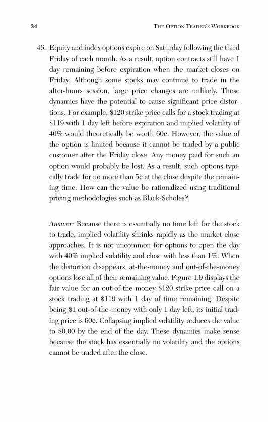
46. Equity and index options expire on Saturday following the thirdFriday of each month. As a result, option contracts still have 1day remaining before expiration when the market closes onFriday. Although some stocks may continue to trade in theafter-hours session, large price changes are unlikely. Thesedynamics have the potential to cause significant price distor-tions. For example, $120 strike price calls for a stock trading at$119 with 1 day left before expiration and implied volatility of40% would theoretically be worth 60¢. However, the value ofthe option is limited because it cannot be traded by a publiccustomer after the Friday close. Any money paid for such anoption would probably be lost. As a result, such options typi-cally trade for no more than 5¢ at the close despite the remain-ing time. How can the value be rationalized using traditionalpricing methodologies such as Black-Scholes?
Answer: Because there is essentially no time left for the stockto trade, implied volatility shrinks rapidly as the market closeapproaches. It is not uncommon for options to open the daywith 40% implied volatility and close with less than 1%. Whenthe distortion disappears, at-the-money and out-of-the-moneyoptions lose all of their remaining value. Figure 1.9 displays thefair value for an out-of-the-money $120 strike price call on astock trading at $119 with 1 day of time remaining. Despitebeing $1 out-of-the-money with only 1 day left, its initial trad-ing price is 60¢. Collapsing implied volatility reduces the valueto $0.00 by the end of the day. These dynamics make sensebecause the stock has essentially no volatility and the optionscannot be traded after the close.
34 THE OPTION TRADER’S WORKBOOK
From the Library of Melissa Wong
ptg
Figure 1.9 Fair trading price versus implied volatility for a $1 out-of-the-money call option on the final trading day of an expiration cycle. Callprices are displayed on the x-axis, volatility on the y-axis.
47. Suppose you were short $100 strike price calls and $90 strikeprice puts on a stock that traded at $95 at the close on expira-tion Friday—that is, both options were $5 out-of-the-money.Why might it be unwise to leave these options assuming theywill expire worthless?
Answer: The underlying stock could react to news that isreleased after the market closes and the options, which arelikely to be in the hands of a broker, can be exercised on Satur-day. Even if the stock does not trade in the Friday after-hourssession, the anticipation of a large move on Monday can driveexecution, forcing the trade to be covered at a substantial lossusing Monday’s stock prices.
CHAPTER 1 • PRICING BASICS 35
0.000
0.050
0.100
0.150
0.200
0.250
0.300
0.350
0.400
0.450
$0.00$0.10 -$0.10$0.20$0.30$0.40$0.50$0.60
From the Library of Melissa Wong
ptg
48. Investors often use options to create “synthetic stock”positions. Which of the following positions is equivalent to 100shares of a stock trading at $100?
A. 1 long $100 call + 1 short $100 put
B. 1 long $105 call + 1 short $95 put
C. 1 long $95 call + 1 short $100 put
Answer: A—1 long $100 call + 1 short $100 put is equivalent to100 shares of stock.
49. With regard to question #48, can you explain why only the firstchoice is correct? Hint: The delta of an at-the-money call isroughly 0.50, and the corresponding put has a delta of –0.50.
Answer: The long call is equivalent to 50 shares of stock (0.5delta × 100 shares per contract). On the put side we are short anegative delta, which is equivalent to being long. Because thesame math applies, the put position is also equivalent to 50shares of long stock. Adding together the number of delta-equivalent shares for both sides gives us a value of 100 shares.
Each of the other choices includes options with a net deltagreater or less than 1.
36 THE OPTION TRADER’S WORKBOOK
From the Library of Melissa Wong
ptg
50. Would the $100 strike price call/put combination of question#49 have still equaled 100 shares of stock if the underlying hadbeen trading at $103?
Answer: Yes. Both deltas would have been shifted by an equiv-alent amount. The following table presents an example. Thefirst pair of entries displays the value of a position that is short10 puts and long 10 calls using the $100 strike with the stocktrading at $103. The second pair of entries reveals the newprice after a $3 increase in the underlying stock price. Bothpositions are built around 35% volatility, 28 days remainingbefore expiration, and a risk-free interest rate of 3.5%.
Stock 10 Contr. Price ($) Call ($) Put ($) Delta Value Net ($)
103.00 5.77 0.65 5,770
103.00 2.50 –0.35 –2,500 3,270
106.00 7.87 0.75 7,870
106.00 1.61 –0.25 –1,610 6,260
Note that a $3 increase in the underlying stock price increasedthe value of the position $2,990, from $3,270 to $6,260. Thischange almost exactly equals that of 1,000 shares of stock.
CHAPTER 1 • PRICING BASICS 37
From the Library of Melissa Wong
ptg
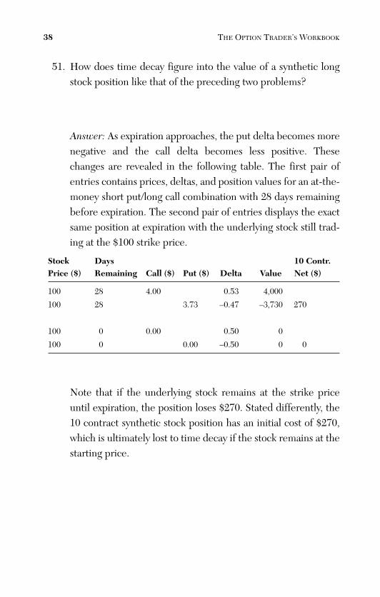
51. How does time decay figure into the value of a synthetic longstock position like that of the preceding two problems?
Answer: As expiration approaches, the put delta becomes morenegative and the call delta becomes less positive. Thesechanges are revealed in the following table. The first pair ofentries contains prices, deltas, and position values for an at-the-money short put/long call combination with 28 days remainingbefore expiration. The second pair of entries displays the exactsame position at expiration with the underlying stock still trad-ing at the $100 strike price.
Stock Days 10 Contr. Price ($) Remaining Call ($) Put ($) Delta Value Net ($)
100 28 4.00 0.53 4,000
100 28 3.73 –0.47 –3,730 270
100 0 0.00 0.50 0
100 0 0.00 –0.50 0 0
Note that if the underlying stock remains at the strike priceuntil expiration, the position loses $270. Stated differently, the10 contract synthetic stock position has an initial cost of $270,which is ultimately lost to time decay if the stock remains at thestarting price.
38 THE OPTION TRADER’S WORKBOOK
From the Library of Melissa Wong
ptg
52. Can you calculate the underlying stock price increase thatwould be necessary to offset the $270 loss in question #51?
Answer: Because a 10 contract position is equivalent to 1,000shares, we would need only a 27¢ increase in the underlyingstock price (0.27 × 10 contracts × 100 shares per contract). Thissimple calculation works because on any given day—includingexpiration day—the position behaves as if it were stock. If thestock closed 27¢ in-the-money at expiration, the call would beworth 27¢ and the put would be worth $0.00. The final positionwould then be worth $270—exactly the time value of the origi-nal trade.
53. Does the synthetic stock position of the preceding five ques-tions have a collateral requirement? (Assume stock trading at$100, 10 short $100 puts, 10 long $100 calls.)
Answer: Yes. Because the puts are uncovered, the requirementis equal to 20% of the value of the underlying stock plus therevenue realized from the short sale. The base requirementwould be 1,000 shares × 0.20 × $100 per share = $20,000.Adding the sale price of the options increases the value by$3.73 × 1,000 = $3,730. Total required collateral is, therefore,$23,730.
CHAPTER 1 • PRICING BASICS 39
From the Library of Melissa Wong
ptg
54. Based on the answer to question #53, can you estimate the“opportunity” cost associated with this trade? (Opportunitycost is related to interest that could be earned on money thatmust be set aside to capitalize the trade in addition to any lossesincurred.)
Answer: The trade has an opportunity cost equal to the following:
Interest on $23,730 collateral
Interest on $4,000 for the long call purchase
Loss of $270 from time decay
Assuming 3.5% interest, the trade would cost approximately$351 for 1 month. One year of interest would be equal to .035× ($23,730 + $4,000) = $970.55. Dividing by 12 and adding the$270 time decay loss gives ($970.55 / 12) + $270 = $350.88.
55. Based on the answer to question #54, how does the cost of asynthetic long stock position compare to actually owning thestock?
Answer: 1,000 shares of a $100 stock would cost $100,000. The1 month opportunity cost of this trade at 3.5% would be$292—slightly less than the cost of the synthetic position. Themajor cost of the synthetic position is the $270 of time decayinherent to the structure.
40 THE OPTION TRADER’S WORKBOOK
From the Library of Melissa Wong
ptg
56. If the synthetic position has a slightly higher cost of ownership,why would an investor not simply buy the stock?
Answer: The synthetic 1,000 share position outlined in the pre-vious questions can be purchased using less than $30,000. Thestock position would cost more than three times as much. How-ever, if the stock could be purchased on margin, it would costonly $50,000 in addition to interest charged by the broker. At3.5%, the 1 month interest charge would be ($50,000 × 0.035) /12 = $146. The ability to exploit margin borrowing dramaticallyreduces the acquisition cost.
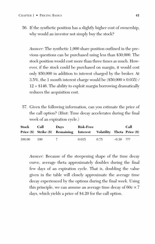
57. Given the following information, can you estimate the price ofthe call option? (Hint: Time decay accelerates during the finalweek of an expiration cycle.)
Stock Call Days Risk-Free Call Price ($) Strike ($) Remaining Interest Volatility Theta Price ($)
100.00 100 7 0.015 0.75 –0.30 ???
Answer: Because of the steepening shape of the time decaycurve, average theta approximately doubles during the finalfew days of an expiration cycle. That is, doubling the valuegiven in the table will closely approximate the average timedecay experienced by the options during the final week. Usingthis principle, we can assume an average time decay of 60¢ × 7days, which yields a price of $4.20 for the call option.
CHAPTER 1 • PRICING BASICS 41
From the Library of Melissa Wong
ptg
Summary
This chapter was designed to provide a series of practical exer-cises that highlight important aspects of option pricing theory. It wasmeant to complement the many excellent texts that already exist onthe subject, in addition to hundreds of academic research papers.Modern option pricing began with the publication of the Black-Scholes formula in 1973. Today, more than 35 years later, this elegantformula still forms the foundation of most option pricing activities. Inthis context we should distinguish between the price of an option andits value. Option pricing theory, including Black-Scholes and itsextensions, can be used to determine the value of an option; the mar-ket determines its actual trading price. Sometimes the two differ con-siderably. For example, during early 2008 the implied volatility ofoptions on financial stocks climbed steeply as a sub-prime lending cri-sis generated billions of dollars of losses among these institutions. Inmany cases actual prices were no longer based on historical volatilityof the underlying stocks, but on the market’s perception of risk. Plug-ging actual trading prices into the Black-Scholes formula sometimesgave implied volatilities of more than 500%. Furthermore, the volatil-ity smile—an important extension to the Black-Scholes model—steepened considerably causing out-of-the-money put options to bepriced with even higher implied volatilities. Such distortions are thesource of pricing theory refinements that allow the market to accom-modate unusual situations.
The calculations used throughout this book are based on theBlack-Scholes formula. Many of the problems extend the model withimplied volatilities that vary across different strike prices and expira-tion dates in addition to unique situations such as the dividend arbi-trage scenario outlined at the end of Chapter 5, “Complex Trades—Part 2.” Although the chapters can be reviewed in any order, theywere designed as a progression that begins with long put and callpositions and progresses to complex multipart trades spanning differ-ent strike prices and expiration dates. In all cases the goal was to cre-ate scenarios that can be addressed using basic principles.
42 THE OPTION TRADER’S WORKBOOK
From the Library of Melissa Wong
ptg
Purchasing Puts and Calls
Simply stated, purchasing a call is a directional bet with higherleverage than an equivalent stock purchase. Purchasing puts is equiv-alent to shorting stock. Long puts and calls have many advantagesover stock. Most notable is the flexibility to use different strike pricesand expiration dates to accommodate a variety of expectations for theperformance of the underlying stock. “Bullish” and “bearish” arebroad terms, and the simple purchase or short sale of a stock does notadequately represent all bullish or bearish views. Suppose, for exam-ple, that you believe a stock might suddenly rise sharply as the resultof an impending news event. That expectation is much different froma long-term somewhat positive view that can be summarized with thephrase “good long-term investment.” Skillful call buying strategiescan be tailored to accommodate either view.
Call and put buying also has the advantage of leverage, a dynamicthat ultimately impacts the size of a portfolio that can be purchased.Consider the difficulties faced by an investor trying to purchase a port-folio of stocks with $10,000. A single trade consisting of 100 shares of a$100 stock would consume the entire budget. The same amount ofmoney, however, could purchase a fairly broad portfolio of calls acrossmany different securities. This approach allows an investor to use callsto gain exposure to expensive large cap stocks without bearing the pro-hibitive costs usually associated with owning those stocks. The samecan obviously be said for buying puts versus shorting stocks. Short saleshave margin requirements that are generally much larger than the costof purchasing an equivalent portfolio of puts.
2
43
From the Library of Melissa Wong
ptg
Skillfully choosing the right mix of long and short-dated expira-tions and strike prices allows an investor to distribute risk, maximizeprofit, and capitalize on different types of price change behavior.Even more important is the ability to respond with a corrective strat-egy when a stock moves the wrong way. For example, stock ownershave only two choices for responding to a price decline: sell some orall of the stock, or buy more to “average down” the purchase price.Neither is a particularly good choice. Option traders have far betterchoices that involve shifting to different strike prices and/or sellingcalls to offset some of the loss. An option trader can recover from aloss, sometimes with a profit, even if the stock never returns to itsprevious price. Option traders can also take advantage of strategiesthat lock in profits after a sharp rise or fall. Stock investors are limitedhere as well because their only choice is to sell some or all of theirstock or, in the case of a short position, to cover all or some of theirtrade. With luck the stock will reverse direction and provide a newtrading opportunity.
In this section we will explore the dynamics associated with pur-chasing and owning puts and calls. Many of the questions will involvethe kind of adjustments mentioned previously. Strictly speaking,these discussions reach beyond the basics of call and put buying intothe realm of position management. Such extensions are appropriatebecause every option purchased must eventually be sold, and thejump to selling additional contracts as position adjustments is rela-tively small. These discussions are also intended as an introduction tomore complex position management scenarios that will be exploredin later sections.
44 THE OPTION TRADER’S WORKBOOK
From the Library of Melissa Wong
ptg
Basic Dynamics (Problems #1–#7)
1. Suppose you buy $100 strike price calls for $2.50. Assumingthat you hold the position until expiration, what price must theunderlying stock achieve on expiration day for your trade tobreak even?
Answer: $102.50.
2. Most option positions are not held until expiration becauselarge upward or downward spikes usually intervene. Supposeyou purchased 10 contacts of a call option for $1.50 and thestock spiked upward, driving the price to $3.75. An excellentstrategy might be to sell enough of the contracts to pay for theoriginal trade and hold the remainder in anticipation of furtherincreases. How many contracts would you need to sell to payfor the original trade?
Answer: 4 contracts. The original trade cost $1.50 × 10 con-tracts × 100 shares per contract = $1,500. Selling 4 contractsfor $3.75 would recover the entire $1,500 ($3.75 × 4 contracts× 100 shares per contract).
CHAPTER 2 • PURCHASING PUTS AND CALLS 45
From the Library of Melissa Wong
ptg
3. Would you be more likely to hold the remaining 6 contracts ifthe spike occurred near or far from expiration?
Answer: As expiration approaches, time decay accelerates, andthe chance of additional large upward spikes shrinks rapidlywith each passing day. In the final few days it almost nevermakes sense to continue holding option contracts that have alarge profit. Suppose, for example, that the large upward spikewas 3 standard deviations and only 5 days remain before expira-tion. It is very unlikely that two spikes of this magnitude willoccur within one week. Additionally, regression toward themean often erodes some of the gain as other investors takeprofit and the stock sells off. If the large upward spike occurs inthe after- or before-hours session, it would be wise to close theoptions as soon as the market opens. Finally, if the stock is farin-the-money close to expiration, the option will have a delta of1.0 and the decision to continue holding the option is tanta-mount to holding an equivalent number of shares of the under-lying stock. Most option positions are not designed to besynthetic stock and, therefore, should not be held when theydisplay that characteristic.
4. The term “leverage” is often misused. Generally speaking, acall owner will realize greater percentage gains and losses thana stockholder for the same size movement of the underlyingbecause the call provides greater leverage. Which of the follow-ing long call positions provides greater leverage?
A. 100 contracts costing $0.24/$10 out-of-the-money
B. 10 contracts costing $2.57/at-the-money
46 THE OPTION TRADER’S WORKBOOK
From the Library of Melissa Wong
ptg
Answer: A—$0.24 option/$10 out-of-the-money provides muchmore leverage. The following table contains the sample tradesused to structure this question. Implied volatility was set at35%, 70 days remained before expiration, and the risk freeinterest rate was 3.5%.
Stock ($) Strike ($) Call ($)
40 50 0.24
40 40 2.57
45 50 1.14
45 40 6.03
In the second pair of entries, the stock has risen from $40 to$45. At-the-money options have more than doubled from $2.57to $6.03, and out-of-the-money options have more thanquadrupled from $0.24 to $1.14.
5. Would the results in question #4 have changed if the scenarioplayed out with half as much time left (35 days) in the optioncontracts?
Answer: The exaggeration increases sharply as expirationapproaches. In this particular case, an option pricing calculatorcan be used to show that the at-the-money $40 calls wouldincrease in value from $1.79 to $5.44 (3 times), while the out-of-the-money $50 calls would increase a much larger percent-age from 4¢ to 48¢ (12 times).
CHAPTER 2 • PURCHASING PUTS AND CALLS 47
From the Library of Melissa Wong
ptg
6. Why does the comparison break down when the time left isreduced to just a few days?
Answer: Except in situations where implied volatility is extraor-dinarily high, options that are 25% out-of-the-money are value-less with only a few days left. As expiration approaches,out-of-the-money leverage continues to increase until a point isreached where even a large move of the underlying fails toaffect the nearest strike price. For example, with impliedvolatility of 35% and the stock trading at $40, a 1 standard devi-ation 3-day price change would be just $1.28. The positionwould, therefore, be 7.9 standard deviations out-of-the-money.The calculation is as follows:
Timeframes in 1 year 365/3 = 121.67
Annualization factor Sqrt (121.67) =11.03
Volatility for 3 days 0.35 / 11.03 = 0.032
1 StdDev change 0.032 × $40 = $1.28
Because the chance of a 7.9 standard deviation change is van-ishingly small, the $50 calls would have virtually no value withthe stock trading at $40 and only 3 days left before expiration.
7. Leverage can be deceiving because it works in percentagesrather than absolute amounts. In question #4 we compared theperformance of out-of-the-money and at-the-money options fora stock whose price increased $5. With 70 days remaining beforeexpiration, $10 out-of-the-money calls climbed from $0.24 to$1.14 while the value of at-the-money calls increased from $2.57to $6.03. In percentage terms, the value of out-of-the-moneyoptions increased 375% while at-the-money options climbed amore modest 135%. In absolute terms, however, at-the-moneyoptions gained considerably more. If the at-the-money invest-ment was 10 contracts, how many out-of-the-money contractswould you need to achieve the same absolute gain?
48 THE OPTION TRADER’S WORKBOOK
From the Library of Melissa Wong
ptg
Answer: Approximately 38 contracts. The comparison is dis-played in the following table (OTM = out-of-the-money, ATM= at-the-money).
OTM Call ($) 38 Contracts ($) Gain ($)
0.24 912
1.14 4,332 3,420
ATM Call ($) 10 Contracts ($) Gain ($)
2.57 2,570
6.03 6,030 3,460
At-the-money calls gained $3,460. Because the out-of-the-money calls grew in value by $0.90 ($90 per contract), we candivide to find the appropriate number of contracts:
$3,460 / $90 per contract = 38.4 contracts
Protecting Profit (Problems #8–#19)
There is no shortage of frustrated investors who, after making awise and profitable investment, have experienced losses because theyfailed to protect their profit. The problem often occurs when a stockrallies early in an expiration cycle before falling back below the origi-nal price. Furthermore, because options experience time decay, astock can rally during the early part of the cycle and the profit can belost by expiration if the price does not continue climbing. The follow-ing problems were designed to address a variety of basic conceptssurrounding profit protection for simple long call positions. (All calcu-lations in this section are based on a 3.5% risk-free interest rate.)
CHAPTER 2 • PURCHASING PUTS AND CALLS 49
From the Library of Melissa Wong
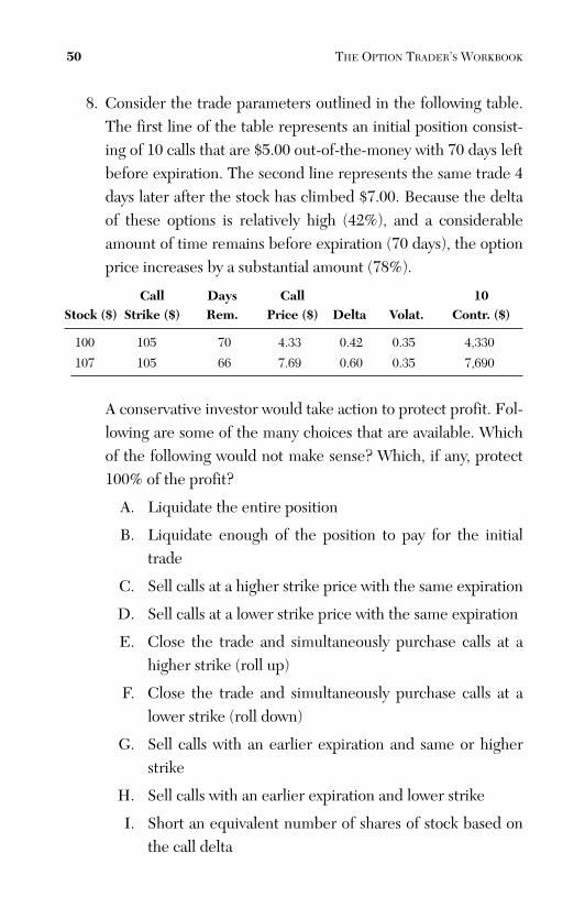
ptg
8. Consider the trade parameters outlined in the following table.The first line of the table represents an initial position consist-ing of 10 calls that are $5.00 out-of-the-money with 70 days leftbefore expiration. The second line represents the same trade 4days later after the stock has climbed $7.00. Because the deltaof these options is relatively high (42%), and a considerableamount of time remains before expiration (70 days), the optionprice increases by a substantial amount (78%).
Call Days Call 10 Stock ($) Strike ($) Rem. Price ($) Delta Volat. Contr. ($)
100 105 70 4.33 0.42 0.35 4,330
107 105 66 7.69 0.60 0.35 7,690
A conservative investor would take action to protect profit. Fol-lowing are some of the many choices that are available. Whichof the following would not make sense? Which, if any, protect100% of the profit?
A. Liquidate the entire position
B. Liquidate enough of the position to pay for the initialtrade
C. Sell calls at a higher strike price with the same expiration
D. Sell calls at a lower strike price with the same expiration
E. Close the trade and simultaneously purchase calls at ahigher strike (roll up)
F. Close the trade and simultaneously purchase calls at alower strike (roll down)
G. Sell calls with an earlier expiration and same or higherstrike
H. Sell calls with an earlier expiration and lower strike
I. Short an equivalent number of shares of stock based onthe call delta
50 THE OPTION TRADER’S WORKBOOK
From the Library of Melissa Wong
ptg
Answer: Liquidating the entire position (choice A) is the onlychoice that protects 100% of the profit under all circumstances.Choices D, F, and H do not make sense. D and H each involvecreating a bearish position by selling more valuable calls thathave a higher delta and a lower strike price. Each of thesetrades would profit from a price decline of the underlying.Choice F increases exposure to downward moves of the under-lying by creating a more expensive long position with a higherdelta. In this scenario all the profit remains at risk in addition tothe added cost of the new trade.
Rolling up to a higher strike (E) can lock in some of the profitby creating a new lower-cost position similar to the initial trade.The amount of profit that is protected depends on the amountof money put at risk in the new position.
Selling calls at a higher strike price (C) and selling calls with thesame or higher strike price and an earlier expiration (G) aresimilar strategies in that each protects some of the profit.Unlike rolling up, these strategies cap the potential gainbecause they contain a short component.
Liquidating enough of the position to pay for the initial trade(B) prevents an overall loss but leaves all the profit at risk.
Shorting an equivalent amount of stock as measured by thedelta (I) creates a position similar to a long straddle. Additionalprofit would be generated by either a sharp increase or sharpdecline in the stock price. Alternatively, a reduced number ofshares can be shorted as a hedge against a price reversal. Thenumber of shares chosen should reflect the investor’s level ofbullishness. One solution is to short enough shares of stock tocreate a position with a net delta equal to that of the originaltrade.
CHAPTER 2 • PURCHASING PUTS AND CALLS 51
From the Library of Melissa Wong
ptg
9. Suppose that after the large price spike in question #8 youdecided to keep the position unchanged—that is, long 10 callsat the $105 strike price with the stock trading at $107. Howmany stock-equivalent shares would you be long? How do thecosts of the two positions compare?
Answer: 10 contracts with a delta of 0.60 is equivalent to 600shares of stock. Since the stock is trading at $107, the costwould be $107 × 600 = $64,200. From the table in question #8,we know that the options are worth $7,690.
10. Why, in question #9, would an investor be willing to pay$64,200 for stock that is fundamentally equivalent to a $7,690option position? Can you compare the values of the two posi-tions if the stock falls $2.00 and continues trading at the strikeprice until expiration? How would the positions compare if thestock remained at $107 until expiration?
Answer: If the underlying falls $2.00 and remains at or belowthe strike price until expiration, the entire $7,690 would be lost.The same price decline would generate a loss of only $1,200 foran investor holding 600 shares of stock.
If the stock remains $2.00 in-the-money until expiration, theoption trade will lose $5.69 while the stock position will not loseanything.
11. If you kept the position until expiration, the stock remained at$107, and you didn’t sell any offsetting calls, would you have aprofit?
52 THE OPTION TRADER’S WORKBOOK
From the Library of Melissa Wong
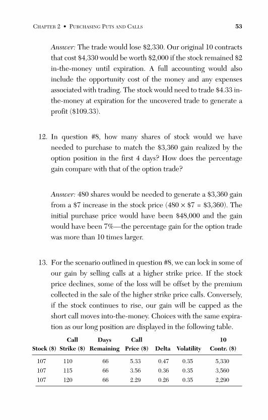
ptg
Answer: The trade would lose $2,330. Our original 10 contractsthat cost $4,330 would be worth $2,000 if the stock remained $2in-the-money until expiration. A full accounting would alsoinclude the opportunity cost of the money and any expensesassociated with trading. The stock would need to trade $4.33 in-the-money at expiration for the uncovered trade to generate aprofit ($109.33).
12. In question #8, how many shares of stock would we haveneeded to purchase to match the $3,360 gain realized by theoption position in the first 4 days? How does the percentagegain compare with that of the option trade?
Answer: 480 shares would be needed to generate a $3,360 gainfrom a $7 increase in the stock price (480 × $7 = $3,360). Theinitial purchase price would have been $48,000 and the gainwould have been 7%—the percentage gain for the option tradewas more than 10 times larger.
13. For the scenario outlined in question #8, we can lock in some ofour gain by selling calls at a higher strike price. If the stockprice declines, some of the loss will be offset by the premiumcollected in the sale of the higher strike price calls. Conversely,if the stock continues to rise, our gain will be capped as theshort call moves into-the-money. Choices with the same expira-tion as our long position are displayed in the following table.
Call Days Call 10 Stock ($) Strike ($) Remaining Price ($) Delta Volatility Contr. ($)
107 110 66 5.33 0.47 0.35 5,330
107 115 66 3.56 0.36 0.35 3,560
107 120 66 2.29 0.26 0.35 2,290
CHAPTER 2 • PURCHASING PUTS AND CALLS 53
From the Library of Melissa Wong
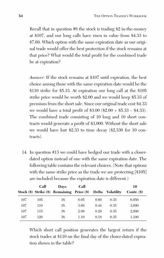
ptg
Recall that in question #8 the stock is trading $2 in-the-moneyat $107, and our long calls have risen in value from $4.33 to$7.69. Which option with the same expiration date as our origi-nal trade would offer the best protection if the stock remains atthat price? What would the total profit for the combined tradebe at expiration?
Answer: If the stock remains at $107 until expiration, the bestchoice among those with the same expiration date would be the$110 strike for $5.33. At expiration our long call at the $105strike price would be worth $2.00 and we would keep $5.33 ofpremium from the short sale. Since our original trade cost $4.33we would have a total profit of $3.00 ($2.00 + $5.33 – $4.33).The combined trade consisting of 10 long and 10 short con-tracts would generate a profit of $3,000. Without the short salewe would have lost $2.33 to time decay ($2,330 for 10 con-tracts).
14. In question #13 we could have hedged our trade with a closer-dated option instead of one with the same expiration date. Thefollowing table contains the relevant choices. (Note that optionswith the same strike price as the trade we are protecting [$105]are included because the expiration date is different.)
Call Days Call 10 Stock ($) Strike ($) Remaining Price ($) Delta Volatility Contr. ($)
107 105 38 6.05 0.60 0.35 6,050
107 110 38 3.69 0.44 0.35 3,690
107 115 38 2.09 0.29 0.35 2,090
107 120 38 1.10 0.18 0.35 1,100
Which short call position generates the largest return if thestock trades at $110 on the final day of the closer-dated expira-tion shown in the table?
54 THE OPTION TRADER’S WORKBOOK
From the Library of Melissa Wong
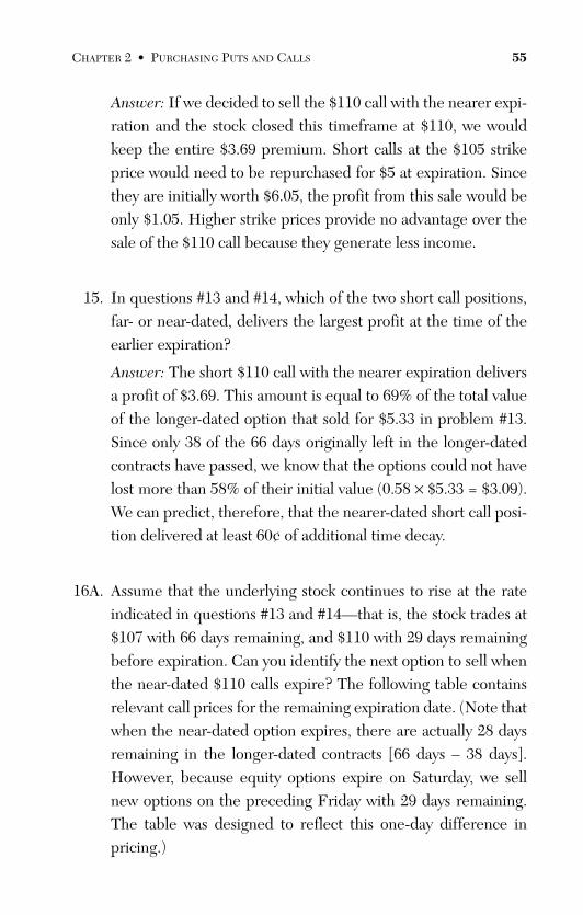
ptg
Answer: If we decided to sell the $110 call with the nearer expi-ration and the stock closed this timeframe at $110, we wouldkeep the entire $3.69 premium. Short calls at the $105 strikeprice would need to be repurchased for $5 at expiration. Sincethey are initially worth $6.05, the profit from this sale would beonly $1.05. Higher strike prices provide no advantage over thesale of the $110 call because they generate less income.
15. In questions #13 and #14, which of the two short call positions,far- or near-dated, delivers the largest profit at the time of theearlier expiration?
Answer: The short $110 call with the nearer expiration deliversa profit of $3.69. This amount is equal to 69% of the total valueof the longer-dated option that sold for $5.33 in problem #13.Since only 38 of the 66 days originally left in the longer-datedcontracts have passed, we know that the options could not havelost more than 58% of their initial value (0.58 × $5.33 = $3.09).We can predict, therefore, that the nearer-dated short call posi-tion delivered at least 60¢ of additional time decay.
16A. Assume that the underlying stock continues to rise at the rateindicated in questions #13 and #14—that is, the stock trades at$107 with 66 days remaining, and $110 with 29 days remainingbefore expiration. Can you identify the next option to sell whenthe near-dated $110 calls expire? The following table containsrelevant call prices for the remaining expiration date. (Note thatwhen the near-dated option expires, there are actually 28 daysremaining in the longer-dated contracts [66 days – 38 days].However, because equity options expire on Saturday, we sellnew options on the preceding Friday with 29 days remaining.The table was designed to reflect this one-day difference inpricing.)
CHAPTER 2 • PURCHASING PUTS AND CALLS 55
From the Library of Melissa Wong
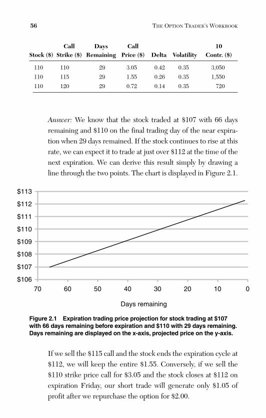
ptg
Call Days Call 10 Stock ($) Strike ($) Remaining Price ($) Delta Volatility Contr. ($)
110 110 29 3.05 0.42 0.35 3,050
110 115 29 1.55 0.26 0.35 1,550
110 120 29 0.72 0.14 0.35 720
Answer: We know that the stock traded at $107 with 66 daysremaining and $110 on the final trading day of the near expira-tion when 29 days remained. If the stock continues to rise at thisrate, we can expect it to trade at just over $112 at the time of thenext expiration. We can derive this result simply by drawing aline through the two points. The chart is displayed in Figure 2.1.
56 THE OPTION TRADER’S WORKBOOK
$106
$107
$108
$109
$110
$111
$112
$113
010203040506070
Days remaining
Figure 2.1 Expiration trading price projection for stock trading at $107with 66 days remaining before expiration and $110 with 29 days remaining.Days remaining are displayed on the x-axis, projected price on the y-axis.
If we sell the $115 call and the stock ends the expiration cycle at$112, we will keep the entire $1.55. Conversely, if we sell the$110 strike price call for $3.05 and the stock closes at $112 onexpiration Friday, our short trade will generate only $1.05 ofprofit after we repurchase the option for $2.00.
From the Library of Melissa Wong
ptg
16B. Assuming that we follow the path implied by question #16A—that is, we hedge our long $105 call position by first selling $110calls with 38 days remaining and then $115 calls when the firsthedge expires—what will our total profit be if the stock closesthe final expiration cycle at $112?
Answer: $7.91 ($7,910 for 10 contracts). Our long position isworth $7.00 at expiration with the underlying stock trading at$112. Additionally, we sold 2 sets of options including $110 callsfor $3.69 and $115 calls for $1.55. Total revenue for the trade,therefore, is $7.00 + $3.69 + $1.55 = $12.24. We must subtractthe cost of our original long position to obtain the final profit($12.24 – $4.33 = $7.91). If each trade in the sequence involved10 contracts, our total profit would be $7,910. Calculated as apercentage of the initial trade, the profit would be 183%.
17. In questions #15 and #16 we used a line drawn through twoprice points to predict that the stock would trade below $115 atthe end of the expiration cycle. Is this assumption reasonablegiven the implied volatility listed in the accompanying table(35%)?
Answer: The table lists implied volatility as 35%. With 29 daysremaining and the stock trading at $110, we can calculate thesize of a 1 standard deviation change as follows:
Timeframes in 1 year 365 / 29 = 12.59 timeframes
Annualization factor Sqrt (12.58) = 3.55
Volatility for 29 days 0.35 / 3.55 = .099
1 StdDev change .099 × $110 = $10.89
CHAPTER 2 • PURCHASING PUTS AND CALLS 57
From the Library of Melissa Wong
ptg
If the implied volatility is appropriate, then a $5 price increaseto $115 during the remaining 29 days represents a change ofonly about half of a standard deviation. The normal distributionpredicts that 62% of all price changes will be larger than 0.5standard deviations. Statistically, however, half of these can beexpected to be price increases and half will be decreases. Usingthe normal distribution, we can estimate that the probability ofthe stock trading above $115 at expiration is only 31%. Thisnumber can be arrived at using Excel’s normal distributionfunction or a table in a statistics textbook.
In the case of Excel, the function NORMSDIST(0.5) = 0.691.This result represents the percentage of price changes for the29-day timeframe that fall below +0.5 standard deviations.Because half the changes are negative, we can subtract these todetermine the percentage that falls between 0.0 and +0.5(0.691 – 0.50 = 0.191). The remaining 31% of the positivechanges lie above +0.5 StdDev.
18. In question #8 after the rapid increase to $107, how manyshares would we need to short to create a delta-neutral positionthat exactly offsets the long calls? How many shares would weneed to short to create a long position that is delta-equivalent tothe original trade?
Answer: 600 shares of stock would offset 10 calls with a delta of0.60 (10 contracts × 100 shares per contract × 0.60). Alterna-tively, shorting 180 shares of stock would reduce the effectivedelta from 0.60 to 0.42, the value of the original trade.
58 THE OPTION TRADER’S WORKBOOK
From the Library of Melissa Wong
ptg
19. If we created the delta-neutral position described in question#18 and the stock fell $10, would the complete set of trades beprofitable at expiration? If so, what would the percent gain beon an annual basis?
Answer: Yes. If the price fell $10, the short stock trade wouldgain $6,000 and our original long call position, which cost$4,330, would expire worthless. The combination would yield aprofit of $1,670. The gain would be 2.4% calculated as follows:$1,670 profit / ($66,000 short stock + $4,330 long calls). Sincethere were 66 days remaining before expiration, we can annual-ize the number by multiplying by 365 / 66. Without compound-ing, the result would be 13.3% per year.
Defensive Action (Problems #20–#38)
The previous set of problems focused on strategies for protectingprofit. Although this problem is a good one to have, we must also beprepared to take defensive action to recover from losses. The follow-ing problems address basic issues surrounding such strategies. (Allcalculations in this section are based on a 3.5% risk-free interest rate.)
20. Consider the trade parameters outlined in the following table.The first line of the table represents an initial position consist-ing of 10 calls that are $5.00 out-of-the-money with 70 days leftbefore expiration. The second line represents the same trade 4days later after the stock has fallen $7.00. Because the delta ofthese options is relatively high (42%), and a considerableamount of time remains before expiration (70 days), the optionprice decreases by a substantial amount (57%).
CHAPTER 2 • PURCHASING PUTS AND CALLS 59
From the Library of Melissa Wong
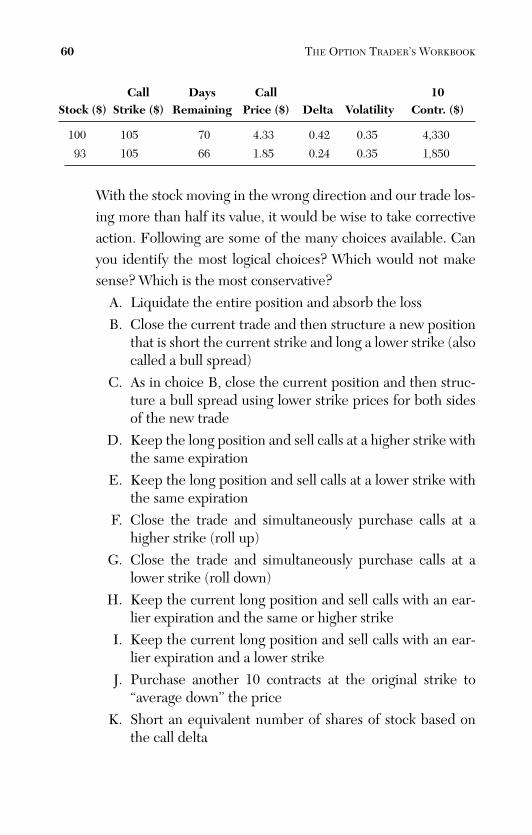
ptg
Call Days Call 10 Stock ($) Strike ($) Remaining Price ($) Delta Volatility Contr. ($)
100 105 70 4.33 0.42 0.35 4,330
93 105 66 1.85 0.24 0.35 1,850
With the stock moving in the wrong direction and our trade los-ing more than half its value, it would be wise to take correctiveaction. Following are some of the many choices available. Canyou identify the most logical choices? Which would not makesense? Which is the most conservative?
A. Liquidate the entire position and absorb the lossB. Close the current trade and then structure a new position
that is short the current strike and long a lower strike (alsocalled a bull spread)
C. As in choice B, close the current position and then struc-ture a bull spread using lower strike prices for both sidesof the new trade
D. Keep the long position and sell calls at a higher strike withthe same expiration
E. Keep the long position and sell calls at a lower strike withthe same expiration
F. Close the trade and simultaneously purchase calls at ahigher strike (roll up)
G. Close the trade and simultaneously purchase calls at alower strike (roll down)
H. Keep the current long position and sell calls with an ear-lier expiration and the same or higher strike
I. Keep the current long position and sell calls with an ear-lier expiration and a lower strike
J. Purchase another 10 contracts at the original strike to“average down” the price
K. Short an equivalent number of shares of stock based onthe call delta
60 THE OPTION TRADER’S WORKBOOK
From the Library of Melissa Wong
ptg
Answer: Liquidating the entire position (choice A) is the onlychoice that prevents any further losses. As such it is the mostconservative choice. Choices E and I do not make sensebecause they create bearish positions by selling more valuablecalls that have a higher delta and a lower strike price. Each ofthese trades would profit if the underlying stock declines.While such a strategy might make sense for a stock that hasrecently fallen sharply, there are more efficient ways to struc-ture a bearish position. It is unlikely that we would keep ourlong $105 strike price calls as part of a bearish structure.
Choice G increases exposure to downward moves of the under-lying by creating a more expensive long position with a higherdelta. If the stock continues to decline, our losses would bemagnified. Very aggressive investors sometimes take thisapproach because they count on mean reversion, a force thatcan sometimes reverse a sharp decline. Choice J is philosophi-cally similar—a very bullish investor might consider the declinean opportunity to purchase additional contracts at a reducedprice. This approach should be considered only by investorswho limit their original purchase and can accept a larger loss onthe combined trade.
Rolling up to a higher strike (F) limits further losses by reduc-ing the cost of the position. However, it generally does notmake sense to purchase farther out-of-the-money calls on astock that is declining.
Choices B, C, D, and H are logical solutions for an investor whoremains bullish. Each creates a new trade structure that lowersthe break-even point while capping the potential gain. Some,but not all, reduce the maximum possible loss. With each struc-ture it is possible to recover the full loss and realize a profit atexpiration.
CHAPTER 2 • PURCHASING PUTS AND CALLS 61
From the Library of Melissa Wong
ptg
As before, shorting a delta-equivalent number of shares (K)creates a position that embodies many of the dynamics of a longstraddle. Profit would be generated by either a sharp increaseor sharp decline in the stock price. The number of shares canbe calibrated to reflect the investor’s level of bullishness orbearishness; a bullish investor might short a small number ofshares as a hedge, whereas a more bearish investor would likelyselect enough shares to match the delta of the stock. A verybearish investor might short more shares than required tomatch the delta of the calls. In the new bearish position theexisting calls would serve as a hedge to protect the short stockposition in the event of a price increase.
21. How many stock-equivalent shares were represented in theoriginal trade? How many are represented in the same positionafter the $7 price decline?
Answer: The original position was equivalent to 420 shares ofstock. After the decline, at a delta of 0.24, the position repre-sents only 240 shares of stock.
22. Which would have suffered the greater loss, 420 shares of stockor the original long call position consisting of 10 contracts at the$105 strike price? Why is there a difference if the positions aredelta-equivalent?
Answer: The stock position would have lost $2,940 ($7 × 420shares) while the long calls would have lost only $2,480. Thestock position suffers a greater loss because its delta is always1.0, whereas the call delta continually declines as the underly-ing moves away from the strike price.
62 THE OPTION TRADER’S WORKBOOK
From the Library of Melissa Wong
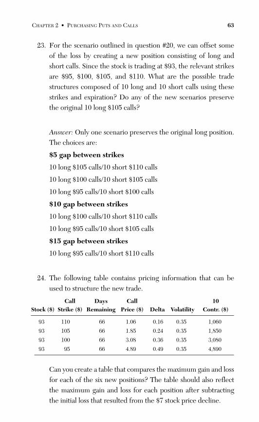
ptg
23. For the scenario outlined in question #20, we can offset someof the loss by creating a new position consisting of long andshort calls. Since the stock is trading at $93, the relevant strikesare $95, $100, $105, and $110. What are the possible tradestructures composed of 10 long and 10 short calls using thesestrikes and expiration? Do any of the new scenarios preservethe original 10 long $105 calls?
Answer: Only one scenario preserves the original long position.The choices are:
$5 gap between strikes
10 long $105 calls/10 short $110 calls
10 long $100 calls/10 short $105 calls
10 long $95 calls/10 short $100 calls
$10 gap between strikes
10 long $100 calls/10 short $110 calls
10 long $95 calls/10 short $105 calls
$15 gap between strikes
10 long $95 calls/10 short $110 calls
24. The following table contains pricing information that can beused to structure the new trade.
Call Days Call 10 Stock ($) Strike ($) Remaining Price ($) Delta Volatility Contr. ($)
93 110 66 1.06 0.16 0.35 1,060
93 105 66 1.85 0.24 0.35 1,850
93 100 66 3.08 0.36 0.35 3,080
93 95 66 4.89 0.49 0.35 4,890
Can you create a table that compares the maximum gain and lossfor each of the six new positions? The table should also reflectthe maximum gain and loss for each position after subtractingthe initial loss that resulted from the $7 stock price decline.
CHAPTER 2 • PURCHASING PUTS AND CALLS 63
From the Library of Melissa Wong
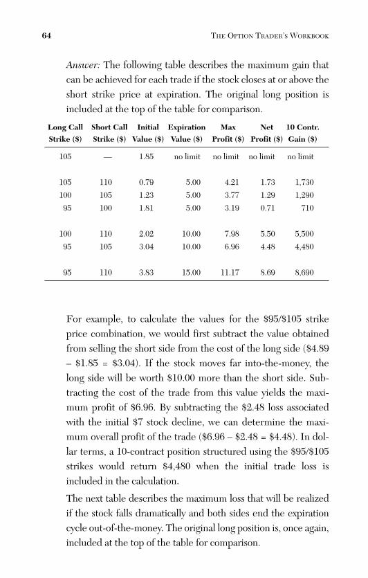
ptg
Answer: The following table describes the maximum gain thatcan be achieved for each trade if the stock closes at or above theshort strike price at expiration. The original long position isincluded at the top of the table for comparison.
Long Call Short Call Initial Expiration Max Net 10 Contr.
Strike ($) Strike ($) Value ($) Value ($) Profit ($) Profit ($) Gain ($)
105 — 1.85 no limit no limit no limit no limit
105 110 0.79 5.00 4.21 1.73 1,730
100 105 1.23 5.00 3.77 1.29 1,290
95 100 1.81 5.00 3.19 0.71 710
100 110 2.02 10.00 7.98 5.50 5,500
95 105 3.04 10.00 6.96 4.48 4,480
95 110 3.83 15.00 11.17 8.69 8,690
For example, to calculate the values for the $95/$105 strikeprice combination, we would first subtract the value obtainedfrom selling the short side from the cost of the long side ($4.89– $1.85 = $3.04). If the stock moves far into-the-money, thelong side will be worth $10.00 more than the short side. Sub-tracting the cost of the trade from this value yields the maxi-mum profit of $6.96. By subtracting the $2.48 loss associatedwith the initial $7 stock decline, we can determine the maxi-mum overall profit of the trade ($6.96 – $2.48 = $4.48). In dol-lar terms, a 10-contract position structured using the $95/$105strikes would return $4,480 when the initial trade loss isincluded in the calculation.
The next table describes the maximum loss that will be realizedif the stock falls dramatically and both sides end the expirationcycle out-of-the-money. The original long position is, once again,included at the top of the table for comparison.
64 THE OPTION TRADER’S WORKBOOK
From the Library of Melissa Wong
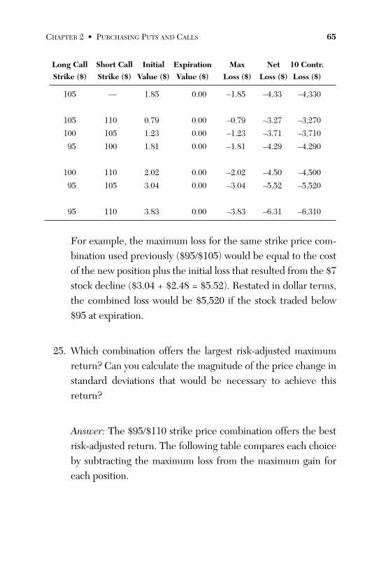
ptg
Long Call Short Call Initial Expiration Max Net 10 Contr.
Strike ($) Strike ($) Value ($) Value ($) Loss ($) Loss ($) Loss ($)
105 — 1.85 0.00 –1.85 –4.33 –4,330
105 110 0.79 0.00 –0.79 –3.27 –3,270
100 105 1.23 0.00 –1.23 –3.71 –3,710
95 100 1.81 0.00 –1.81 –4.29 –4,290
100 110 2.02 0.00 –2.02 –4.50 –4,500
95 105 3.04 0.00 –3.04 –5.52 –5,520
95 110 3.83 0.00 –3.83 –6.31 –6,310
For example, the maximum loss for the same strike price com-bination used previously ($95/$105) would be equal to the costof the new position plus the initial loss that resulted from the $7stock decline ($3.04 + $2.48 = $5.52). Restated in dollar terms,the combined loss would be $5,520 if the stock traded below$95 at expiration.
25. Which combination offers the largest risk-adjusted maximumreturn? Can you calculate the magnitude of the price change instandard deviations that would be necessary to achieve thisreturn?
Answer: The $95/$110 strike price combination offers the bestrisk-adjusted return. The following table compares each choiceby subtracting the maximum loss from the maximum gain foreach position.
CHAPTER 2 • PURCHASING PUTS AND CALLS 65
From the Library of Melissa Wong
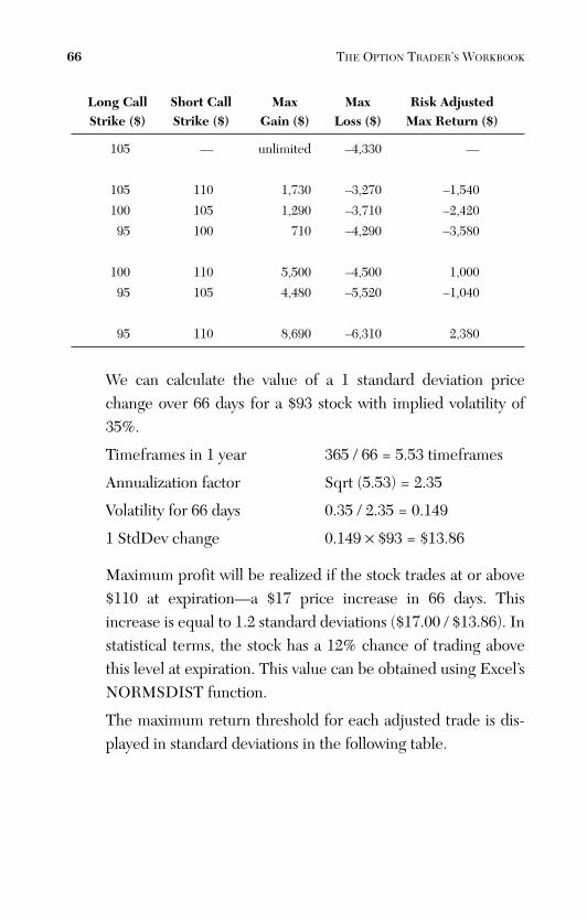
ptg
Long Call Short Call Max Max Risk Adjusted Strike ($) Strike ($) Gain ($) Loss ($) Max Return ($)
105 — unlimited –4,330 —
105 110 1,730 –3,270 –1,540
100 105 1,290 –3,710 –2,420
95 100 710 –4,290 –3,580
100 110 5,500 –4,500 1,000
95 105 4,480 –5,520 –1,040
95 110 8,690 –6,310 2,380
We can calculate the value of a 1 standard deviation pricechange over 66 days for a $93 stock with implied volatility of35%.
Timeframes in 1 year 365 / 66 = 5.53 timeframes
Annualization factor Sqrt (5.53) = 2.35
Volatility for 66 days 0.35 / 2.35 = 0.149
1 StdDev change 0.149 × $93 = $13.86
Maximum profit will be realized if the stock trades at or above$110 at expiration—a $17 price increase in 66 days. Thisincrease is equal to 1.2 standard deviations ($17.00 / $13.86). Instatistical terms, the stock has a 12% chance of trading abovethis level at expiration. This value can be obtained using Excel’sNORMSDIST function.
The maximum return threshold for each adjusted trade is dis-played in standard deviations in the following table.
66 THE OPTION TRADER’S WORKBOOK
From the Library of Melissa Wong
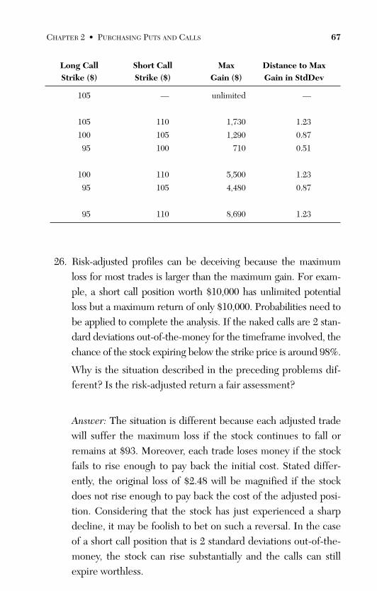
ptg
Long Call Short Call Max Distance to Max Strike ($) Strike ($) Gain ($) Gain in StdDev
105 — unlimited —
105 110 1,730 1.23
100 105 1,290 0.87
95 100 710 0.51
100 110 5,500 1.23
95 105 4,480 0.87
95 110 8,690 1.23
26. Risk-adjusted profiles can be deceiving because the maximumloss for most trades is larger than the maximum gain. For exam-ple, a short call position worth $10,000 has unlimited potentialloss but a maximum return of only $10,000. Probabilities need tobe applied to complete the analysis. If the naked calls are 2 stan-dard deviations out-of-the-money for the timeframe involved, thechance of the stock expiring below the strike price is around 98%.
Why is the situation described in the preceding problems dif-ferent? Is the risk-adjusted return a fair assessment?
Answer: The situation is different because each adjusted tradewill suffer the maximum loss if the stock continues to fall orremains at $93. Moreover, each trade loses money if the stockfails to rise enough to pay back the initial cost. Stated differ-ently, the original loss of $2.48 will be magnified if the stockdoes not rise enough to pay back the cost of the adjusted posi-tion. Considering that the stock has just experienced a sharpdecline, it may be foolish to bet on such a reversal. In the caseof a short call position that is 2 standard deviations out-of-the-money, the stock can rise substantially and the calls can stillexpire worthless.
CHAPTER 2 • PURCHASING PUTS AND CALLS 67
From the Library of Melissa Wong
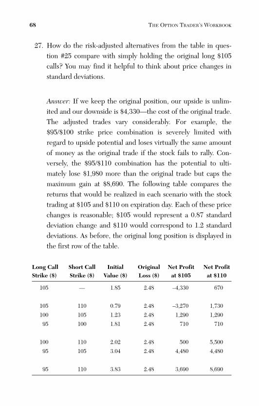
ptg
27. How do the risk-adjusted alternatives from the table in ques-tion #25 compare with simply holding the original long $105calls? You may find it helpful to think about price changes instandard deviations.
Answer: If we keep the original position, our upside is unlim-ited and our downside is $4,330—the cost of the original trade.The adjusted trades vary considerably. For example, the$95/$100 strike price combination is severely limited withregard to upside potential and loses virtually the same amountof money as the original trade if the stock fails to rally. Con-versely, the $95/$110 combination has the potential to ulti-mately lose $1,980 more than the original trade but caps themaximum gain at $8,690. The following table compares thereturns that would be realized in each scenario with the stocktrading at $105 and $110 on expiration day. Each of these pricechanges is reasonable; $105 would represent a 0.87 standarddeviation change and $110 would correspond to 1.2 standarddeviations. As before, the original long position is displayed inthe first row of the table.
Long Call Short Call Initial Original Net Profit Net Profit Strike ($) Strike ($) Value ($) Loss ($) at $105 at $110
105 — 1.85 2.48 –4,330 670
105 110 0.79 2.48 –3,270 1,730
100 105 1.23 2.48 1,290 1,290
95 100 1.81 2.48 710 710
100 110 2.02 2.48 500 5,500
95 105 3.04 2.48 4,480 4,480
95 110 3.83 2.48 3,690 8,690
68 THE OPTION TRADER’S WORKBOOK
From the Library of Melissa Wong
ptg
Profit for each row is calculated by subtracting the original lossplus the cost of the new trade from the value of the position atexpiration. For example, the $95/$105 combination had an ini-tial cost of $3.04. Adding the previous loss of $2.48 provides uswith the total cost that must be recovered for the trade to beprofitable ($5.52). At expiration with the stock trading at $105,the long $95 calls would be worth $10 and the short $105 callswould expire worthless—the position would be worth $10. Sub-tracting the cost that must be recovered including the originalloss yields a profit of $4.48, or $4,480 for 10 contracts. Becausethe long and short sides of the trade are both in-the-money, fur-ther increases in the price of the underlying stock have noeffect.
Despite having unlimited potential upside, the original longposition yields the lowest return of the group for modestincreases in the underlying stock price. At $105, the originaltrade suffers the greatest loss—$4,330—and at $110 it barelygenerates any profit. Conversely, the most profitable trade at$105 is the $95/$105 combination because the long side isworth $10 and the short side expires worthless. The samedynamics cause the $95/$110 combination to deliver the largestprofit if the stock closes at $110 on expiration day.
28. At what expiration price does the original trade become thebest alternative? How many standard deviations must the stockmove to reach this price?
Answer: The largest maximum gain for any of the adjusted posi-tions is $11.17 for the $95/$110 combination with the stocktrading at, or above, $110 on expiration day. The original tradewill not generate this much profit unless the underlying stockrises to $120.50 by expiration. This value is obtained by addingthe required profit ($11.17) to the initial cost ($4.33 including
CHAPTER 2 • PURCHASING PUTS AND CALLS 69
From the Library of Melissa Wong
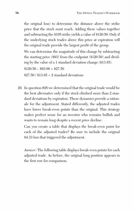
ptg
the original loss) to determine the distance above the strikeprice that the stock must reach. Adding these values togetherand subtracting the $105 strike yields a value of $120.50. Only ifthe underlying stock trades above this price at expiration willthe original trade provide the largest profit of the group.
We can determine the magnitude of this change by subtractingthe starting price ($93) from the endpoint ($120.50) and divid-ing by the value of a 1 standard deviation change ($13.85).
$120.50 – $93.00 = $27.50
$27.50 / $13.85 = 2 standard deviations
29. In question #28 we determined that the original trade would bethe best alternative only if the stock climbed more than 2 stan-dard deviations by expiration. These dynamics provide a ration-ale for the adjustment. Stated differently, the adjusted tradeshave lower break-even points than the original. This strategymakes perfect sense for an investor who remains bullish andwants to remain long despite a recent price decline.
Can you create a table that displays the break-even point foreach of the adjusted trades? Be sure to include the original$4.33 loss that triggered the adjustment.
Answer: The following table displays break-even points for eachadjusted trade. As before, the original long position appears inthe first row for comparison.
70 THE OPTION TRADER’S WORKBOOK
From the Library of Melissa Wong
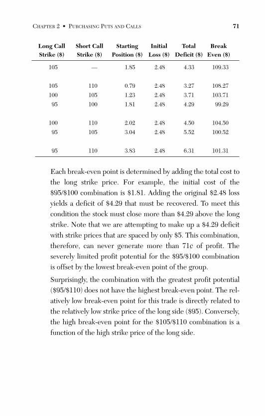
ptg
CHAPTER 2 • PURCHASING PUTS AND CALLS 71
Long Call Short Call Starting Initial Total Break Strike ($) Strike ($) Position ($) Loss ($) Deficit ($) Even ($)
105 — 1.85 2.48 4.33 109.33
105 110 0.79 2.48 3.27 108.27
100 105 1.23 2.48 3.71 103.71
95 100 1.81 2.48 4.29 99.29
100 110 2.02 2.48 4.50 104.50
95 105 3.04 2.48 5.52 100.52
95 110 3.83 2.48 6.31 101.31
Each break-even point is determined by adding the total cost tothe long strike price. For example, the initial cost of the$95/$100 combination is $1.81. Adding the original $2.48 lossyields a deficit of $4.29 that must be recovered. To meet thiscondition the stock must close more than $4.29 above the longstrike. Note that we are attempting to make up a $4.29 deficitwith strike prices that are spaced by only $5. This combination,therefore, can never generate more than 71¢ of profit. Theseverely limited profit potential for the $95/$100 combinationis offset by the lowest break-even point of the group.
Surprisingly, the combination with the greatest profit potential($95/$110) does not have the highest break-even point. The rel-atively low break-even point for this trade is directly related tothe relatively low strike price of the long side ($95). Conversely,the high break-even point for the $105/$110 combination is afunction of the high strike price of the long side.
From the Library of Melissa Wong
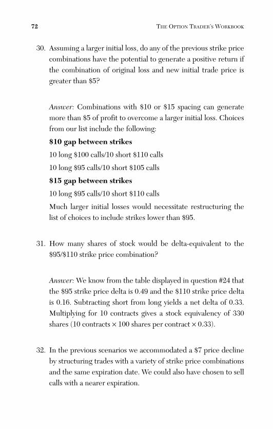
ptg
30. Assuming a larger initial loss, do any of the previous strike pricecombinations have the potential to generate a positive return ifthe combination of original loss and new initial trade price isgreater than $5?
Answer: Combinations with $10 or $15 spacing can generatemore than $5 of profit to overcome a larger initial loss. Choicesfrom our list include the following:
$10 gap between strikes
10 long $100 calls/10 short $110 calls
10 long $95 calls/10 short $105 calls
$15 gap between strikes
10 long $95 calls/10 short $110 calls
Much larger initial losses would necessitate restructuring thelist of choices to include strikes lower than $95.
31. How many shares of stock would be delta-equivalent to the$95/$110 strike price combination?
Answer: We know from the table displayed in question #24 thatthe $95 strike price delta is 0.49 and the $110 strike price deltais 0.16. Subtracting short from long yields a net delta of 0.33.Multiplying for 10 contracts gives a stock equivalency of 330shares (10 contracts × 100 shares per contract × 0.33).
32. In the previous scenarios we accommodated a $7 price declineby structuring trades with a variety of strike price combinationsand the same expiration date. We could also have chosen to sellcalls with a nearer expiration.
72 THE OPTION TRADER’S WORKBOOK
From the Library of Melissa Wong
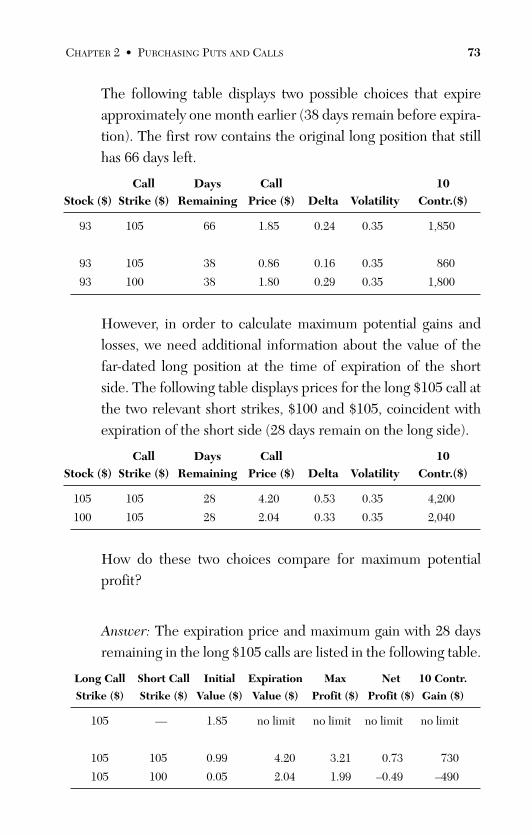
ptg
The following table displays two possible choices that expireapproximately one month earlier (38 days remain before expira-tion). The first row contains the original long position that stillhas 66 days left.
Call Days Call 10 Stock ($) Strike ($) Remaining Price ($) Delta Volatility Contr.($)
93 105 66 1.85 0.24 0.35 1,850
93 105 38 0.86 0.16 0.35 860
93 100 38 1.80 0.29 0.35 1,800
However, in order to calculate maximum potential gains andlosses, we need additional information about the value of thefar-dated long position at the time of expiration of the shortside. The following table displays prices for the long $105 call atthe two relevant short strikes, $100 and $105, coincident withexpiration of the short side (28 days remain on the long side).
Call Days Call 10 Stock ($) Strike ($) Remaining Price ($) Delta Volatility Contr.($)
105 105 28 4.20 0.53 0.35 4,200
100 105 28 2.04 0.33 0.35 2,040
How do these two choices compare for maximum potentialprofit?
Answer: The expiration price and maximum gain with 28 daysremaining in the long $105 calls are listed in the following table.
Long Call Short Call Initial Expiration Max Net 10 Contr.
Strike ($) Strike ($) Value ($) Value ($) Profit ($) Profit ($) Gain ($)
105 — 1.85 no limit no limit no limit no limit
105 105 0.99 4.20 3.21 0.73 730
105 100 0.05 2.04 1.99 –0.49 –490
CHAPTER 2 • PURCHASING PUTS AND CALLS 73
From the Library of Melissa Wong
ptg
Total profit is calculated by subtracting the cost of each tradefrom the maximum value when the short side expires. Reducingthis amount by the original loss ($2.48) yields the net profit. Forexample, selling $105 calls after the initial price decline reducesthe cost of the long side by 86¢ to $0.99. With the short sideexpiring at-the-money, the long $105 calls are worth $4.20.Subtracting the net cost of the original trade (99¢) yields aprofit of $3.21. Further reducing this gain by the amount of theinitial loss ($2.48) yields a net profit of only 73¢ or $730 for 10contracts. Note that if the stock only rises to $100 by the time ofthe near expiration, the long side will not appreciate enough topay back the original $2.48 loss. This result might seem surpris-ing because the short $100 call, which has decayed to zero, ini-tially sold for $1.80—nearly the same price as the long call.
33. Does the $100/$105 combination make any sense if it cannotgenerate a profit? Why would an investor make this adjust-ment?
Answer: It is important to remember that the initial trade lost$2.48 when the stock declined $7. Both trades have the poten-tial to significantly reduce that loss. The $105/$105 combina-tion can fully reverse the loss and generate a profit of $730; the$100/$105 combination can reduce the loss from $2,480 to$490. In return for diminished upside potential, the less favor-able combination offers greater protection if the stock remainsat $93 or falls further.
34. Can the stock rise far enough at any point in the expirationcycle to raise the price of the near-dated $105 call above its far-dated equivalent? Can the two sides achieve the same value?
74 THE OPTION TRADER’S WORKBOOK
From the Library of Melissa Wong
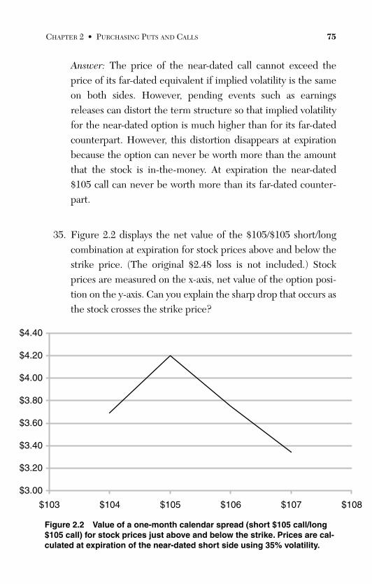
ptg
Answer: The price of the near-dated call cannot exceed theprice of its far-dated equivalent if implied volatility is the sameon both sides. However, pending events such as earningsreleases can distort the term structure so that implied volatilityfor the near-dated option is much higher than for its far-datedcounterpart. However, this distortion disappears at expirationbecause the option can never be worth more than the amountthat the stock is in-the-money. At expiration the near-dated$105 call can never be worth more than its far-dated counter-part.
35. Figure 2.2 displays the net value of the $105/$105 short/longcombination at expiration for stock prices above and below thestrike price. (The original $2.48 loss is not included.) Stockprices are measured on the x-axis, net value of the option posi-tion on the y-axis. Can you explain the sharp drop that occurs asthe stock crosses the strike price?
CHAPTER 2 • PURCHASING PUTS AND CALLS 75
Figure 2.2 Value of a one-month calendar spread (short $105 call/long$105 call) for stock prices just above and below the strike. Prices are cal-culated at expiration of the near-dated short side using 35% volatility.
$3.00
$3.20
$3.40
$3.60
$3.80
$4.00
$4.20
$4.40
$103 $104 $105 $106 $107 $108
From the Library of Melissa Wong
ptg
Answer: The value drops off steeply because the delta of theshort side rises to 1.0 when the underlying stock crosses thestrike price, and the long side, with one month remainingbefore expiration, has a delta of only about half as much (0.53).If the stock trades at or below the strike price, the short side hasno value. The sharp transition from no value and a delta of 0.0to in-the-money value and a delta of 1.0 creates the profile seenin the figure. If the stock climbs far enough, both deltas will riseto 1.0 and both options will have essentially the same value.
36. What is the maximum potential loss for each combination? Ineach case, what conditions cause the maximum loss?
Answer: For the $105/$105 short/long combination, the maxi-mum loss occurs with the stock far below the strike price atexpiration. In this scenario, both sides are worthless and the netcost of the initial trade ($0.99) is lost. The initial value of 99¢ isalso lost if the stock moves very far above the strike price whereboth sides have the same value. In either case, the maximumloss is equal to the original net cost of the position—99¢.
The $100/$105 short/long combination is different because theshort side will be worth $5.00 more than the long side if thestock trades far above the strike price at expiration. In this sce-nario, we would be forced to close the trade and buy back theshort side for a $5.00 loss. Because both sides were initiallyworth approximately the same amount, the $5.00 differencewould be equal to the entire loss. Conversely, if the stock tradesfar below the strike price at expiration, both sides collapse tozero and nothing is lost because the initial trade cost only 5¢.
In summary, both positions experience their maximum loss if thestock trades far above the strike price at expiration—$5.00 for the$100/$105 combination and 99¢ for the position built solelyaround the $105 strike. The single strike position also experiencesits maximum loss if the stock trades far below the strike price.
76 THE OPTION TRADER’S WORKBOOK
From the Library of Melissa Wong
ptg
37. Based on the previous discussion and analysis, which of the twonear-dated adjustments would be more appropriate for astrongly bullish investor—10 short calls at the $105 strike or 10short calls at the $100 strike?
Answer: Shorting the $105 strike is more appropriate for a bull-ish investor because it yields limited losses for very largeincreases of the underlying stock and larger losses in the eventof additional declines. Conversely, the $100 strike is fullyhedged against additional stock declines but provides a muchsmaller return if the stock rises. Worse still, a steep rise in thestock generates a significant loss if the lower strike is shorted. Itis, therefore, difficult to imagine that a bullish investor wouldstructure this position.
38. Assume that we sell the $105 call as our original correction andthe stock climbs to $105 at the time of the near expiration—thatis, we keep the premium from the $105 short call and realize a$3.21 profit on the new trade. How much money is at risk if wekeep the position without selling another hedge in the remain-ing month?
Answer: $4.20 is at risk because that is the value of the far-datedlong $105 call.
CHAPTER 2 • PURCHASING PUTS AND CALLS 77
From the Library of Melissa Wong
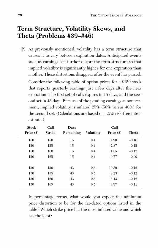
ptg
Term Structure, Volatility Skews, andTheta (Problems #39–#46)
39. As previously mentioned, volatility has a term structure thatcauses it to vary between expiration dates. Anticipated eventssuch as earnings can further distort the term structure so thatimplied volatility is significantly higher for one expiration thananother. These distortions disappear after the event has passed.
Consider the following table of option prices for a $150 stockthat reports quarterly earnings just a few days after the nearexpiration. The first set of calls expires in 15 days, and the sec-ond set in 43 days. Because of the pending earnings announce-ment, implied volatility is inflated 25% (50% versus 40%) forthe second set. (Calculations are based on 1.5% risk-free inter-est rate.)
Stock Call Days Call Price ($) Strike Remaining Volatility Price ($) Theta
150 150 15 0.4 4.90 –0.16
150 155 15 0.4 2.87 –0.15
150 160 15 0.4 1.55 –0.12
150 165 15 0.4 0.77 –0.09
150 150 43 0.5 10.39 –0.12
150 155 43 0.5 8.23 –0.12
150 160 43 0.5 6.43 –0.12
150 165 43 0.5 4.97 –0.11
In percentage terms, what would you expect the minimumprice distortion to be for the far-dated options listed in thetable? Which strike price has the most inflated value and whichhas the least?
78 THE OPTION TRADER’S WORKBOOK
From the Library of Melissa Wong
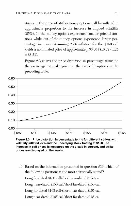
ptg
Answer: The price of at-the-money options will be inflated inapproximate proportion to the increase in implied volatility(25%). In-the-money options experience smaller price distor-tions while out-of-the-money options experience larger per-centage increases. Assuming 25% inflation for the $150 callyields a noninflated price of approximately $8.30 ($10.39 / 1.25= $8.31).
Figure 2.3 charts the price distortion in percentage terms onthe y-axis against strike price on the x-axis for options in thepreceding table.
CHAPTER 2 • PURCHASING PUTS AND CALLS 79
Figure 2.3 Price distortion in percentage terms for different strikes withvolatility inflated 25% and the underlying stock trading at $150.Theincrease in call prices is measured on the y-axis in percent, and strikeprices are displayed on the x-axis.
40. Based on the information presented in question #39, which ofthe following positions is the most statistically sound?
Long far-dated $150 call/short near-dated $150 call
Long near-dated $150 call/short far-dated $150 call
Long far-dated $165 call/short near-dated $165 call
Long near-dated $165 call/short far-dated $165 call
0.00
0.10
0.20
0.30
0.40
0.50
0.60
$135 $140 $145 $150 $155 $160 $165
From the Library of Melissa Wong
ptg
Answer: Long near-dated $165 call/short far-dated $165 callleverages the greatest distortion because the far-dated call isoverpriced by more than 50%. The position is long 40% volatil-ity and short 50%. Another way to think about the trade is thatit is long a $0.77 option and short a $4.97 option that is reallyworth only $3.18. Because of its inflated price, the short far-dated option returns more time decay than its near-dated, cor-rectly priced counterpart. (The short side returns 37% moretime decay than the correctly priced option.)
It is important to realize that the trade dynamics change oncethe near-dated side expires, because rolling forward requirespurchasing expensive current month calls. Additionally, keep-ing the trade open until the distortion-causing event implies acertain level of risk related to the complexities of trading againstan earnings announcement.
Many complex positions can be created to exploit the kinds ofvolatility distortions generated by earnings, expiration, andother special events. It is impossible to fully take advantage ofall the possibilities without considering structures that are bothlong and short, puts and calls across different timeframes. Forexample, in the current scenario we would be much better offselling overpriced far-dated puts and calls against similar cur-rent-month long positions. We could, for example, sell far-dated$165 calls and $145 puts against a long position consisting ofnear-dated options at the same or closer strikes. The dynamicsare complex, and we will return to such structures throughoutthis book in various contexts.
Many investors mistakenly believe that puts are simply theopposite of calls. That view is flawed for two specific reasonsthat are each related to distortions in implied volatility. First,implied volatility tends to rise steeply in response to suddendeclines in the price of the underlying security. This effecttends to magnify the value of a long put position as the stockmoves toward the strike price. Second, out-of-the-money put
80 THE OPTION TRADER’S WORKBOOK
From the Library of Melissa Wong
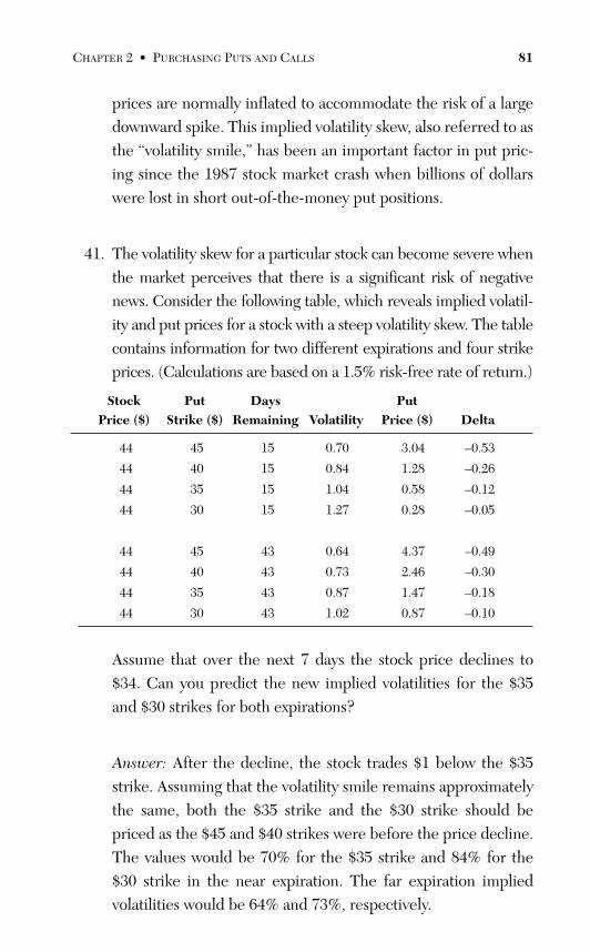
ptg
prices are normally inflated to accommodate the risk of a largedownward spike. This implied volatility skew, also referred to asthe “volatility smile,” has been an important factor in put pric-ing since the 1987 stock market crash when billions of dollarswere lost in short out-of-the-money put positions.
41. The volatility skew for a particular stock can become severe whenthe market perceives that there is a significant risk of negativenews. Consider the following table, which reveals implied volatil-ity and put prices for a stock with a steep volatility skew. The tablecontains information for two different expirations and four strikeprices. (Calculations are based on a 1.5% risk-free rate of return.)
Stock Put Days Put Price ($) Strike ($) Remaining Volatility Price ($) Delta
44 45 15 0.70 3.04 –0.53
44 40 15 0.84 1.28 –0.26
44 35 15 1.04 0.58 –0.12
44 30 15 1.27 0.28 –0.05
44 45 43 0.64 4.37 –0.49
44 40 43 0.73 2.46 –0.30
44 35 43 0.87 1.47 –0.18
44 30 43 1.02 0.87 –0.10
Assume that over the next 7 days the stock price declines to$34. Can you predict the new implied volatilities for the $35and $30 strikes for both expirations?
Answer: After the decline, the stock trades $1 below the $35strike. Assuming that the volatility smile remains approximatelythe same, both the $35 strike and the $30 strike should bepriced as the $45 and $40 strikes were before the price decline.The values would be 70% for the $35 strike and 84% for the$30 strike in the near expiration. The far expiration impliedvolatilities would be 64% and 73%, respectively.
CHAPTER 2 • PURCHASING PUTS AND CALLS 81
From the Library of Melissa Wong
ptg
42. Which of the two $45 strikes would yield the larger profit afterthe price decline—near- or far-dated? What would the approxi-mate prices be?
Answer: Because they are far in-the-money ($11 for a $34stock), both puts can be expected to trade for approximately$11. The near-dated option that traded for $3.04 would have aprofit of $7.96, and the far-dated option would gain $6.63. Inpercentage terms, the near option would gain 262% and the faroption 152%.
43. Using basic principles, can you predict which strike price wouldbe the best investment and which would be the worst for bothexpirations? Why?
Answer: The $40 put was consistently the best investment, andthe $30 put was the worst. If the stock trades for $34 at the time ofthe first expiration, the near-dated $45 put will be worth $11(262% profit), and the near-dated $40 put will be worth $6 (369%profit). The exceptionally large profit of the $40 strike is caused byits transition from $4 out-of-the-money to $6 in-the-money. Thislarge swing causes the delta to fall from –0.26 to –1.0. The deltaswing would be nearly as large with 8 days remaining after the ini-tial downward spike. The $45 option experiences a smaller changein delta because it was initially in-the-money with a delta of –0.53.For the $35 put trading $1 in-the-money, we can estimate that thenew delta will fall between –0.55 and –0.60. This estimate is sup-ported by the delta of the $45 put before the decline (initial deltaof the $35 put was –0.12).
The $30 put loses all its value if it remains out-of-the-money. Italso suffers the largest decrease in implied volatility from 127%to 84%, and the smallest increase in delta (we can estimate themaximum delta from the $40 strike price option before thedecline).
82 THE OPTION TRADER’S WORKBOOK
From the Library of Melissa Wong
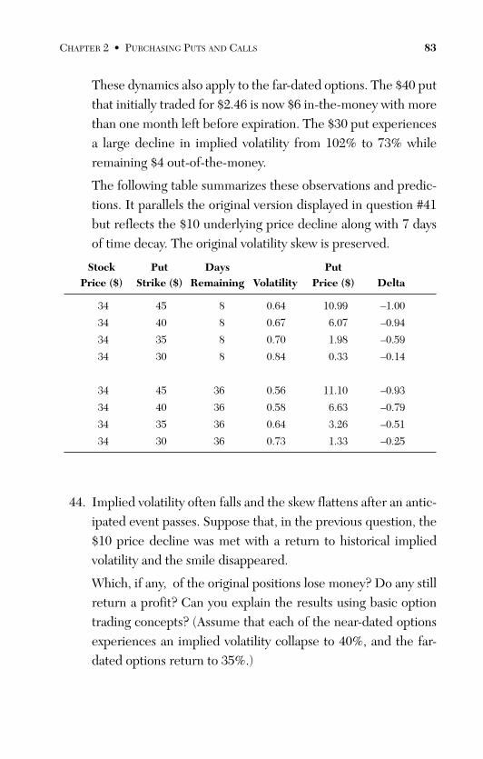
ptg
These dynamics also apply to the far-dated options. The $40 putthat initially traded for $2.46 is now $6 in-the-money with morethan one month left before expiration. The $30 put experiencesa large decline in implied volatility from 102% to 73% whileremaining $4 out-of-the-money.
The following table summarizes these observations and predic-tions. It parallels the original version displayed in question #41but reflects the $10 underlying price decline along with 7 daysof time decay. The original volatility skew is preserved.
Stock Put Days Put Price ($) Strike ($) Remaining Volatility Price ($) Delta
34 45 8 0.64 10.99 –1.00
34 40 8 0.67 6.07 –0.94
34 35 8 0.70 1.98 –0.59
34 30 8 0.84 0.33 –0.14
34 45 36 0.56 11.10 –0.93
34 40 36 0.58 6.63 –0.79
34 35 36 0.64 3.26 –0.51
34 30 36 0.73 1.33 –0.25
44. Implied volatility often falls and the skew flattens after an antic-ipated event passes. Suppose that, in the previous question, the$10 price decline was met with a return to historical impliedvolatility and the smile disappeared.
Which, if any, of the original positions lose money? Do any stillreturn a profit? Can you explain the results using basic optiontrading concepts? (Assume that each of the near-dated optionsexperiences an implied volatility collapse to 40%, and the far-dated options return to 35%.)
CHAPTER 2 • PURCHASING PUTS AND CALLS 83
From the Library of Melissa Wong
ptg
Answer: Because the $45 puts are $11 (24%) in-the-money, wecan safely assume that each trades for very close to $11—a sub-stantial profit for either expiration date. The same dynamicexists for the $40 strike price, which, as previously discussed,generates more profit than the other members of the group.
Because the stock is trading $1 below the $35 strike, we canassume that the $35 put is worth at least $1.00 plus a certainamount of time premium. Original prices for the $35 put withthe stock trading at $44 were $0.58 in the near month and $1.47in the far-dated expiration. All of this value was time premiumbecause the options were $11 out-of-the-money. Even slashingeach value by half still leaves 29¢ of time decay in the nearoption and 70¢ in the far option. Although these are unrealisti-cally low estimates, the near put would still be worth at least$1.29 and its far-dated counterpart at least $1.70. (Actual valuesfor these options are $1.40 and $2.03.)
We can, therefore, assume that each of the first three strikes—$45, $40, $35—generates a positive return in both expirationtimeframes.
The $30 strike is different from the other three because itremains $4 out-of-the-money after the price decline. Because itoriginally had the largest implied volatility, it is also the mostaffected by the newly flattened skew. For comparison purposes,it is helpful to restate distance to the strike in terms of standarddeviations. For the near expiration, the original value is givenby the following:
Timeframes in 1 year 365 / 15 = 24.3 timeframes
Annualization factor Sqrt (24.3) = 4.93
Volatility for 15 days 1.27 / 4.93 = 0.26
1 StdDev change 0.26 × $44 = $11.33
Distance to $30 strike $14/$11.33 = 1.24 StdDev
84 THE OPTION TRADER’S WORKBOOK
From the Library of Melissa Wong
ptg
Although the original price was $14 from the strike, it was only1.24 standard deviations away because of the high volatility(127%). Repeating this calculation with the stock at $34, 8 daysremaining before expiration, and implied volatility of only 40%yields the following:
Timeframes in 1 year 365 / 8 = 45.6 timeframes
Annualization factor Sqrt (45.6) = 6.75
Volatility for 8 days 0.40 / 6.75 = 0.059
1 StdDev change 0.059 × $34 = $2.01
Distance to $30 strike $4/$2.01 = 1.99 StdDev
Surprisingly, in terms of standard deviations the stock is furtherfrom the strike after the price decline than before. Similar dynam-ics hold true for the far-dated option, which begins and ends thescenario approximately 1.1 standard deviations out-of-the-money.
These very rough calculations reveal that the stock has notmoved closer to the strike in option pricing terms. (Actual pric-ing calculations give post-decline values of $0.01 for the near-dated option and $0.22 for the far-dated option.)
45. Unanticipated negative news often causes both a rapid declinein the stock price and a rise in implied volatility. The followingtable depicts such an event in terms of underlying price, volatil-ity, and days remaining before expiration. Four different strikesare shown before and after the drawdown. Predrawdown pricesare given in the table and theta is included for all entries. (Cal-culations are based on a 1.5% risk-free rate of return.)
CHAPTER 2 • PURCHASING PUTS AND CALLS 85
From the Library of Melissa Wong
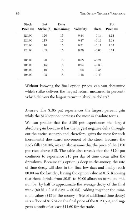
ptg
Stock Put Days Put Price ($) Strike ($) Remaining Volatility Theta Price ($)
120.00 120 15 0.44 –0.14 4.24
120.00 115 15 0.47 –0.13 2.38
120.00 110 15 0.51 –0.11 1.32
120.00 105 15 0.56 –0.08 0.74
105.00 120 8 0.88 –0.21
105.00 115 8 0.94 –0.30
105.00 110 8 1.02 –0.38
105.00 105 8 1.12 –0.43
Without knowing the final option prices, can you determinewhich strike delivers the largest return measured in percent?Which delivers the largest return in absolute dollars?
Answer: The $105 put experiences the largest percent gainwhile the $120 option increases the most in absolute terms.
We can predict that the $120 put experiences the largestabsolute gain because it has the largest negative delta through-out the entire scenario and, therefore, gains the most for eachincremental downward movement of the stock. Because thestock falls to $105, we can also assume that the price of the $120put rises above $15. The table also reveals that the $120 putcontinues to experience 21¢ per day of time decay after thedrawdown. Because this option is deep in-the-money, the rateof time decay will slow in the final few days and finally reach$0.00 on the last day, leaving the option value at $15. Knowingthat theta shrinks from $0.21 to $0.00 allows us to reduce thisnumber by half to approximate the average decay of the finalweek ($0.21 / 2 × 8 days = $0.84). Adding together the mini-mum values ($15 in-the-money + 84¢ of additional time decay)sets a floor of $15.84 on the final price of the $120 put, and sug-gests a profit of at least $11.60 for the trade.
86 THE OPTION TRADER’S WORKBOOK
From the Library of Melissa Wong
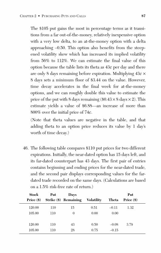
ptg
The $105 put gains the most in percentage terms as it transi-tions from a far out-of-the-money, relatively inexpensive optionwith a very low delta, to an at-the-money option with a deltaapproaching –0.50. This option also benefits from the steep-ened volatility skew which has increased its implied volatilityfrom 56% to 112%. We can estimate the final value of thisoption because the table lists its theta as 43¢ per day and thereare only 8 days remaining before expiration. Multiplying 43¢ ×8 days sets a minimum floor of $3.44 on the value. However,time decay accelerates in the final week for at-the-moneyoptions, and we can roughly double this value to estimate theprice of the put with 8 days remaining ($0.43 × 8 days × 2). Thisestimate yields a value of $6.88—an increase of more than800% over the initial price of 74¢.
(Note that theta values are negative in the table, and thatadding theta to an option price reduces its value by 1 day’sworth of time decay.)
46. The following table compares $110 put prices for two differentexpirations. Initially, the near-dated option has 15 days left, andits far-dated counterpart has 43 days. The first pair of entriescontains beginning and ending prices for the near-dated trade,and the second pair displays corresponding values for the far-dated trade recorded on the same days. (Calculations are basedon a 1.5% risk-free rate of return.)
Stock Put Days Put Price ($) Strike ($) Remaining Volatility Theta Price ($)
120.00 110 15 0.51 –0.11 1.32
105.00 110 0 0.00 0.00
120.00 110 43 0.50 –0.08 3.79
105.00 110 28 0.75 –0.15
CHAPTER 2 • PURCHASING PUTS AND CALLS 87
From the Library of Melissa Wong
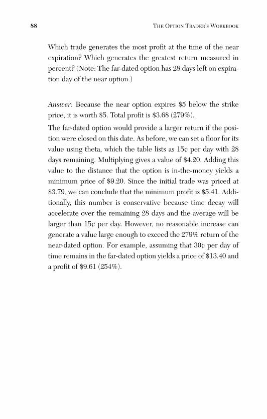
ptg
Which trade generates the most profit at the time of the nearexpiration? Which generates the greatest return measured inpercent? (Note: The far-dated option has 28 days left on expira-tion day of the near option.)
Answer: Because the near option expires $5 below the strikeprice, it is worth $5. Total profit is $3.68 (279%).
The far-dated option would provide a larger return if the posi-tion were closed on this date. As before, we can set a floor for itsvalue using theta, which the table lists as 15¢ per day with 28days remaining. Multiplying gives a value of $4.20. Adding thisvalue to the distance that the option is in-the-money yields aminimum price of $9.20. Since the initial trade was priced at$3.79, we can conclude that the minimum profit is $5.41. Addi-tionally, this number is conservative because time decay willaccelerate over the remaining 28 days and the average will belarger than 15¢ per day. However, no reasonable increase cangenerate a value large enough to exceed the 279% return of thenear-dated option. For example, assuming that 30¢ per day oftime remains in the far-dated option yields a price of $13.40 anda profit of $9.61 (254%).
88 THE OPTION TRADER’S WORKBOOK
From the Library of Melissa Wong
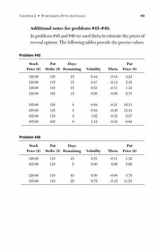
ptg
Additional notes for problems #45–#46:
In problems #45 and #46 we used theta to estimate the prices ofseveral options. The following tables provide the precise values.
Problem #45
Stock Put Days Put Price ($) Strike ($) Remaining Volatility Theta Price ($)
120.00 120 15 0.44 –0.14 4.24
120.00 115 15 0.47 –0.13 2.38
120.00 110 15 0.51 –0.11 1.32
120.00 105 15 0.56 –0.08 0.74
105.00 120 8 0.88 –0.21 16.13
105.00 115 8 0.94 –0.30 12.34
105.00 110 8 1.02 –0.38 9.27
105.00 105 8 1.12 –0.43 6.94
Problem #46
Stock Put Days Put Price ($) Strike ($) Remaining Volatility Theta Price ($)
120.00 110 15 0.51 –0.11 1.32
105.00 110 0 0.00 0.00 5.00
120.00 110 43 0.50 –0.08 3.79
105.00 110 28 0.75 –0.15 11.53
CHAPTER 2 • PURCHASING PUTS AND CALLS 89
From the Library of Melissa Wong
ptg
Summary
Many investors mistakenly believe that puts and calls can be usedas simple proxies for short or long stock positions. This chapter wasdesigned to dispel that belief. Option positions differ from stock posi-tions in many ways—they suffer time decay and eventually expire;they have a threshold or strike price that must be crossed for the con-tracts to have any value at expiration; they provide varying levels ofleverage that can be mathematically described (delta); their valuedepends, in part, on the volatility of the underlying security. Thesecomplex dynamics often lead to the scenario where an investor cor-rectly predicts the direction of a stock but still loses money on whatseems to be a well-planned option trade. Even the simplest trades canbe dynamic and complex to manage.
The discussions in this chapter strayed beyond simple put and callbuying to include hedging and other positional adjustments designedto protect profit. These extensions are intended as a springboard tothe chapters that follow.
90 THE OPTION TRADER’S WORKBOOK
From the Library of Melissa Wong
ptg
Covered Puts and Calls
Covered positions are used by conservative investors who arewilling to accept a cap on their maximum gain in return for a hedgethat can offset potential losses. Covered calls—long stock combinedwith short calls—are the most popular and best understood. Manyinvestors find that covered calls are more profitable than simple longstock positions when the tendency is to hold the stock for a longperiod.
Bearish investors often take the same approach by shorting astock and selling puts. As we will see, covered put positions displaytrading dynamics that are very different from their covered call coun-terparts. Most of the difference is related to spikes in implied volatil-ity that often occur when a stock suddenly falls. Implied volatilityspikes increase the price of the put side of a trade and, therefore,affect the way the trade must be managed.
It is also important to note that covered calls and covered puts arelogically different with regard to the mechanism by which they areexercised. The two sides of a covered call are directly linked; theoption is exercised by calling away the covering stock from theinvestor who sold the call. Conversely, when a put is exercised, theowner sells (puts) the stock to the investor who originally sold theoption. If the original sale was covered with short stock, the investorwho is assigned would simply offset his or her loss by purchasing the
3
91
From the Library of Melissa Wong
ptg
stock that was originally borrowed to create the trade. Both trades arecovered in the sense that no additional collateral is required to pro-tect the short put position.
In the option trading world it is more common to structure cov-ered positions without any stock at all. Long calls substitute for longstock, and long puts replace short stock. A short option position isconsidered covered if the account is long a corresponding number ofoption contracts having more favorable terms—that is, the same orfarther expiration date, and the same or closer strike price. Theserules add additional complexity because the two sides of the trade canhave different expiration dates. Various structures are possible and anappropriate set of names has evolved to describe them. Verticalspreads include long and short options with the same expiration date;calendar spreads span different expirations with the same strike price;diagonals have different strikes and expirations. Generally speaking,it is much more important to understand the trading dynamics ofeach structure than to memorize the names.
Finally, the term “covered” should not be misinterpreted as anindication that uncovered positions are always more dangerous. A sin-gle uncovered short put presents no more risk than 100 shares of longstock. Many investors miss this subtlety and lose the opportunity tocreate a large portfolio that benefits both from price movement andtime decay.
In this section we will explore various covered positions, includ-ing pure option trades that span multiple expirations. We previouslytouched on covered trades in our discussion of simple long call posi-tions. In that context we were either protecting profit after a rally ortaking defensive action in response to a price decline. This sectionbuilds on those discussions with trades that are structured as coveredpositions from the outset. (All calculations for this chapter are basedon a 1.5% risk-free interest rate.)
92 THE OPTION TRADER’S WORKBOOK
From the Library of Melissa Wong
ptg
Traditional Covered Positions InvolvingStock and Options (Problems #1–#23)
1. Which of the following positions are considered covered?(Assume a stock price of $47.)
A. long 1,000 sharesshort 10 contracts—current month $50 call
B. long 1,000 sharesshort 15 contracts—current month $50 call
C. long 1,000 sharesshort 10 contracts—distant month $40 call
D. short 1,000 sharesshort 10 contracts—current month $40 put
E. short 1,000 sharesshort 10 contracts—distant month $60 put
F. long 10 contracts—current month $50 putshort 10 contracts—distant month $50 put
G. long 10 contracts—current month $50 putshort 10 contracts—distant month $40 put
H. long 10 contracts—distant month $70 callshort 10 contracts—current month $60 call
I. long 10 contracts—distant month $60 callshort 10 contracts—current month $60 call
J. long 10 contracts—distant month $50 callshort 10 contracts—current month $55 call
Answer: A, C, D, E, I, and J are covered. B is short 5 extra con-tracts. F and G are short the far-dated option. H is short thecloser strike price. A short position can be covered by an equiv-alent number of shares of stock or the same number of option
CHAPTER 3 • COVERED PUTS AND CALLS 93
From the Library of Melissa Wong
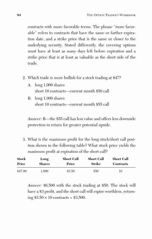
ptg
contracts with more favorable terms. The phrase “more favor-able” refers to contracts that have the same or farther expira-tion date, and a strike price that is the same or closer to theunderlying security. Stated differently, the covering optionsmust have at least as many days left before expiration and astrike price that is at least as valuable as the short side of thetrade.
2. Which trade is more bullish for a stock trading at $47?
A. long 1,000 sharesshort 10 contracts—current month $50 call
B. long 1,000 sharesshort 10 contracts—current month $55 call
Answer: B—the $55 call has less value and offers less downsideprotection in return for greater potential upside.
3. What is the maximum profit for the long stock/short call posi-tion shown in the following table? What stock price yields themaximum profit at expiration of the short call?
Stock Long Short Call Short Call Short Call Price Shares Price Strike Contracts
$47.00 1,000 $3.50 $50 10
Answer: $6,500 with the stock trading at $50. The stock willhave a $3 profit, and the short call will expire worthless, return-ing $3.50 × 10 contracts = $3,500.
94 THE OPTION TRADER’S WORKBOOK
From the Library of Melissa Wong
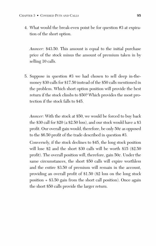
ptg
4. What would the break-even point be for question #3 at expira-tion of the short option.
Answer: $43.50. This amount is equal to the initial purchaseprice of the stock minus the amount of premium taken in byselling 10 calls.
5. Suppose in question #3 we had chosen to sell deep in-the-money $30 calls for $17.50 instead of the $50 calls mentioned inthe problem. Which short option position will provide the bestreturn if the stock climbs to $50? Which provides the most pro-tection if the stock falls to $45.
Answer: With the stock at $50, we would be forced to buy backthe $30 call for $20 (a $2.50 loss), and our stock would have a $3profit. Our overall gain would, therefore, be only 50¢ as opposedto the $6.50 profit of the trade described in question #3.
Conversely, if the stock declines to $45, the long stock positionwill lose $2 and the short $30 calls will be worth $15 ($2.50profit). The overall position will, therefore, gain 50¢. Under thesame circumstances, the short $50 calls will expire worthlessand the entire $3.50 of premium will remain in the account,providing an overall profit of $1.50 ($2 loss on the long stockposition + $3.50 gain from the short call position). Once againthe short $50 calls provide the larger return.
CHAPTER 3 • COVERED PUTS AND CALLS 95
From the Library of Melissa Wong
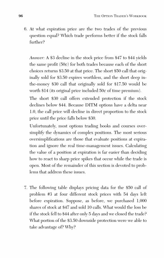
ptg
6. At what expiration price are the two trades of the previousquestion equal? Which trade performs better if the stock fallsfurther?
Answer: A $3 decline in the stock price from $47 to $44 yieldsthe same profit (50¢) for both trades because each of the shortchoices returns $3.50 at that price. The short $50 call that orig-inally sold for $3.50 expires worthless, and the short deep in-the-money $30 call that originally sold for $17.50 would beworth $14 (its original price included 50¢ of time premium).
The short $30 call offers extended protection if the stockdeclines below $44. Because DITM options have a delta near1.0, the call price will decline in direct proportion to the stockprice until the price falls below $30.
Unfortunately, most options trading books and courses over-simplify the dynamics of complex positions. The most seriousoversimplifications are those that evaluate positions at expira-tion and ignore the real time-management issues. Calculatingthe value of a position at expiration is far easier than decidinghow to react to sharp price spikes that occur while the trade isopen. Most of the remainder of this section is devoted to prob-lems that address these issues.
7. The following table displays pricing data for the $50 call ofproblem #3 at four different stock prices with 54 days leftbefore expiration. Suppose, as before, we purchased 1,000shares of stock at $47 and sold 10 calls. What would the loss beif the stock fell to $44 after only 5 days and we closed the trade?What portion of the $3.50 downside protection were we able totake advantage of? Why?
96 THE OPTION TRADER’S WORKBOOK
From the Library of Melissa Wong
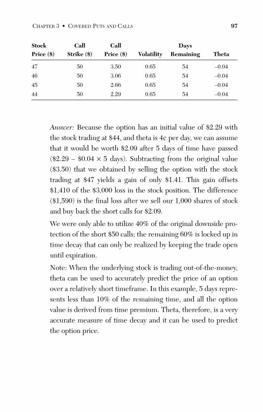
ptg
Stock Call Call Days Price ($) Strike ($) Price ($) Volatility Remaining Theta
47 50 3.50 0.65 54 –0.04
46 50 3.06 0.65 54 –0.04
45 50 2.66 0.65 54 –0.04
44 50 2.29 0.65 54 –0.04
Answer: Because the option has an initial value of $2.29 withthe stock trading at $44, and theta is 4¢ per day, we can assumethat it would be worth $2.09 after 5 days of time have passed($2.29 – $0.04 × 5 days). Subtracting from the original value($3.50) that we obtained by selling the option with the stocktrading at $47 yields a gain of only $1.41. This gain offsets$1,410 of the $3,000 loss in the stock position. The difference($1,590) is the final loss after we sell our 1,000 shares of stockand buy back the short calls for $2.09.
We were only able to utilize 40% of the original downside pro-tection of the short $50 calls; the remaining 60% is locked up intime decay that can only be realized by keeping the trade openuntil expiration.
Note: When the underlying stock is trading out-of-the-money,theta can be used to accurately predict the price of an optionover a relatively short timeframe. In this example, 5 days repre-sents less than 10% of the remaining time, and all the optionvalue is derived from time premium. Theta, therefore, is a veryaccurate measure of time decay and it can be used to predictthe option price.
CHAPTER 3 • COVERED PUTS AND CALLS 97
From the Library of Melissa Wong
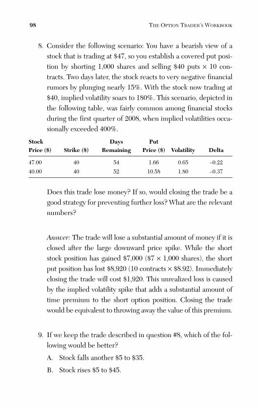
ptg
8. Consider the following scenario: You have a bearish view of astock that is trading at $47, so you establish a covered put posi-tion by shorting 1,000 shares and selling $40 puts × 10 con-tracts. Two days later, the stock reacts to very negative financialrumors by plunging nearly 15%. With the stock now trading at$40, implied volatility soars to 180%. This scenario, depicted inthe following table, was fairly common among financial stocksduring the first quarter of 2008, when implied volatilities occa-sionally exceeded 400%.
Stock Days Put Price ($) Strike ($) Remaining Price ($) Volatility Delta
47.00 40 54 1.66 0.65 –0.22
40.00 40 52 10.58 1.80 –0.37
Does this trade lose money? If so, would closing the trade be agood strategy for preventing further loss? What are the relevantnumbers?
Answer: The trade will lose a substantial amount of money if it isclosed after the large downward price spike. While the shortstock position has gained $7,000 ($7 × 1,000 shares), the shortput position has lost $8,920 (10 contracts × $8.92). Immediatelyclosing the trade will cost $1,920. This unrealized loss is causedby the implied volatility spike that adds a substantial amount oftime premium to the short option position. Closing the tradewould be equivalent to throwing away the value of this premium.
9. If we keep the trade described in question #8, which of the fol-lowing would be better?
A. Stock falls another $5 to $35.
B. Stock rises $5 to $45.
98 THE OPTION TRADER’S WORKBOOK
From the Library of Melissa Wong
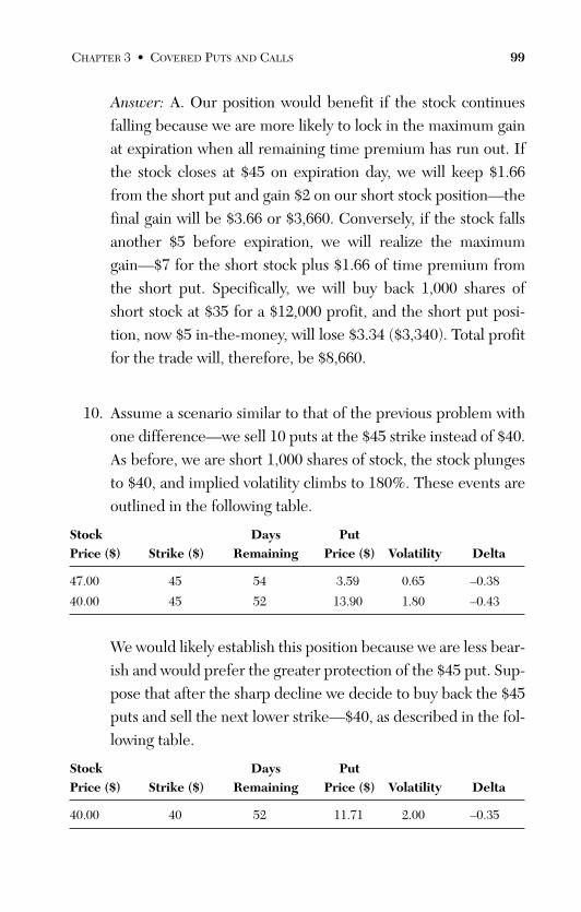
ptg
Answer: A. Our position would benefit if the stock continuesfalling because we are more likely to lock in the maximum gainat expiration when all remaining time premium has run out. Ifthe stock closes at $45 on expiration day, we will keep $1.66from the short put and gain $2 on our short stock position—thefinal gain will be $3.66 or $3,660. Conversely, if the stock fallsanother $5 before expiration, we will realize the maximumgain—$7 for the short stock plus $1.66 of time premium fromthe short put. Specifically, we will buy back 1,000 shares ofshort stock at $35 for a $12,000 profit, and the short put posi-tion, now $5 in-the-money, will lose $3.34 ($3,340). Total profitfor the trade will, therefore, be $8,660.
10. Assume a scenario similar to that of the previous problem withone difference—we sell 10 puts at the $45 strike instead of $40.As before, we are short 1,000 shares of stock, the stock plungesto $40, and implied volatility climbs to 180%. These events areoutlined in the following table.
Stock Days Put Price ($) Strike ($) Remaining Price ($) Volatility Delta
47.00 45 54 3.59 0.65 –0.38
40.00 45 52 13.90 1.80 –0.43
We would likely establish this position because we are less bear-ish and would prefer the greater protection of the $45 put. Sup-pose that after the sharp decline we decide to buy back the $45puts and sell the next lower strike—$40, as described in the fol-lowing table.
Stock Days Put Price ($) Strike ($) Remaining Price ($) Volatility Delta
40.00 40 52 11.71 2.00 –0.35
CHAPTER 3 • COVERED PUTS AND CALLS 99
From the Library of Melissa Wong
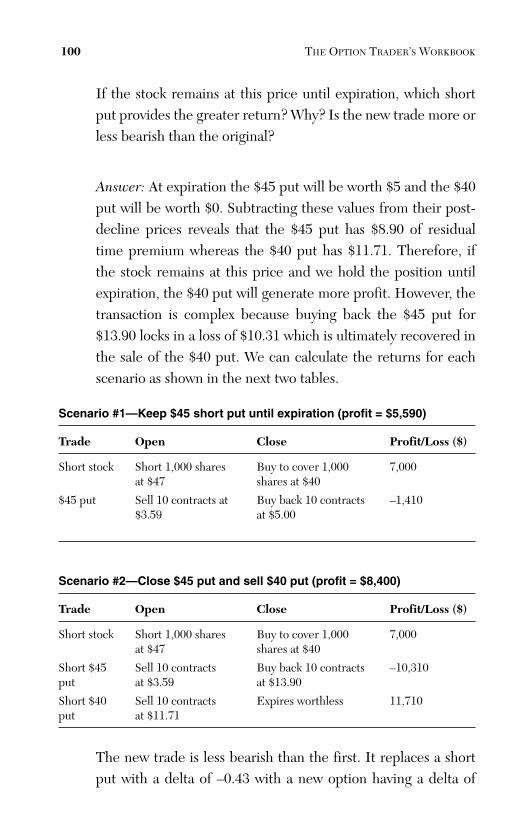
ptg
If the stock remains at this price until expiration, which shortput provides the greater return? Why? Is the new trade more orless bearish than the original?
Answer: At expiration the $45 put will be worth $5 and the $40put will be worth $0. Subtracting these values from their post-decline prices reveals that the $45 put has $8.90 of residualtime premium whereas the $40 put has $11.71. Therefore, ifthe stock remains at this price and we hold the position untilexpiration, the $40 put will generate more profit. However, thetransaction is complex because buying back the $45 put for$13.90 locks in a loss of $10.31 which is ultimately recovered inthe sale of the $40 put. We can calculate the returns for eachscenario as shown in the next two tables.
Scenario #1—Keep $45 short put until expiration (profit = $5,590)
Trade Open Close Profit/Loss ($)
Short stock Short 1,000 shares Buy to cover 1,000 7,000at $47 shares at $40
$45 put Sell 10 contracts at Buy back 10 contracts –1,410$3.59 at $5.00
Scenario #2—Close $45 put and sell $40 put (profit = $8,400)
Trade Open Close Profit/Loss ($)
Short stock Short 1,000 shares Buy to cover 1,000 7,000at $47 shares at $40
Short $45 Sell 10 contracts Buy back 10 contracts –10,310put at $3.59 at $13.90
Short $40 Sell 10 contracts Expires worthless 11,710put at $11.71
The new trade is less bearish than the first. It replaces a shortput with a delta of –0.43 with a new option having a delta of
100 THE OPTION TRADER’S WORKBOOK
From the Library of Melissa Wong
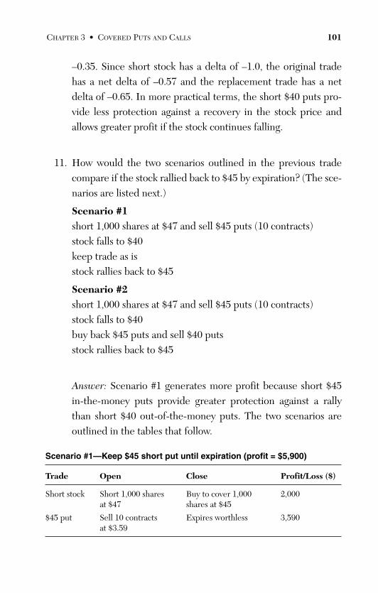
ptg
–0.35. Since short stock has a delta of –1.0, the original tradehas a net delta of –0.57 and the replacement trade has a netdelta of –0.65. In more practical terms, the short $40 puts pro-vide less protection against a recovery in the stock price andallows greater profit if the stock continues falling.
11. How would the two scenarios outlined in the previous tradecompare if the stock rallied back to $45 by expiration? (The sce-narios are listed next.)
Scenario #1short 1,000 shares at $47 and sell $45 puts (10 contracts)stock falls to $40keep trade as isstock rallies back to $45
Scenario #2short 1,000 shares at $47 and sell $45 puts (10 contracts)stock falls to $40buy back $45 puts and sell $40 putsstock rallies back to $45
Answer: Scenario #1 generates more profit because short $45in-the-money puts provide greater protection against a rallythan short $40 out-of-the-money puts. The two scenarios areoutlined in the tables that follow.
Scenario #1—Keep $45 short put until expiration (profit = $5,900)
Trade Open Close Profit/Loss ($)
Short stock Short 1,000 shares Buy to cover 1,000 2,000at $47 shares at $45
$45 put Sell 10 contracts Expires worthless 3,590at $3.59
CHAPTER 3 • COVERED PUTS AND CALLS 101
From the Library of Melissa Wong
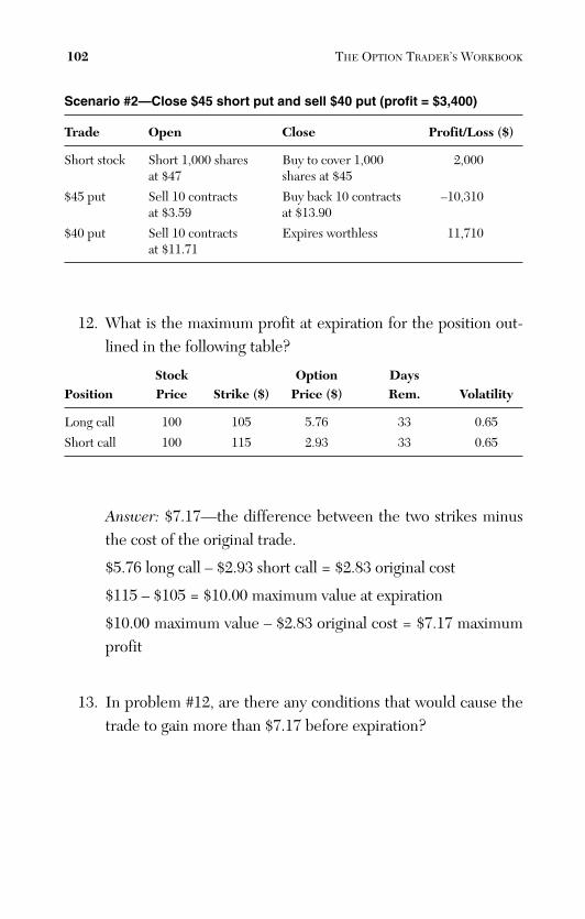
ptg
Scenario #2—Close $45 short put and sell $40 put (profit = $3,400)
Trade Open Close Profit/Loss ($)
Short stock Short 1,000 shares Buy to cover 1,000 2,000at $47 shares at $45
$45 put Sell 10 contracts Buy back 10 contracts –10,310at $3.59 at $13.90
$40 put Sell 10 contracts Expires worthless 11,710at $11.71
12. What is the maximum profit at expiration for the position out-lined in the following table?
Stock Option DaysPosition Price Strike ($) Price ($) Rem. Volatility
Long call 100 105 5.76 33 0.65
Short call 100 115 2.93 33 0.65
Answer: $7.17—the difference between the two strikes minusthe cost of the original trade.
$5.76 long call – $2.93 short call = $2.83 original cost
$115 – $105 = $10.00 maximum value at expiration
$10.00 maximum value – $2.83 original cost = $7.17 maximumprofit
13. In problem #12, are there any conditions that would cause thetrade to gain more than $7.17 before expiration?
102 THE OPTION TRADER’S WORKBOOK
From the Library of Melissa Wong
ptg
Answer: No, the maximum profit can only be obtained at expi-ration with the long call $10 in-the-money and the short callexpiring worthless. No underlying price change at any point inthe expiration cycle can yield a value for the long call that is $10more than the value of the short call. The only exceptions arerelated to large differential volatility swings. The maximumprofit can increase if implied volatility of the long call risessharply relative to that of the short call. Distortions of this mag-nitude are extremely rare.
This section explores scenarios that involve a series of coveredcalls spanning four months. The sequence begins at Decemberexpiration with the stock trading at $104, and ends at April expi-ration with the stock at $108. Many different strike price andexpiration date combinations are possible. We might, for exam-ple, respond to changes in the underlying stock price by sellinga new batch of calls at a different strike each month. Alterna-tively, we could simplify the process by selling April calls onceat the beginning of the process. Selecting the latter option,however, does not rule out the possibility of reacting to changesby adjusting the short call position.
The following table contains relevant pricing information foreach of the four expirations. Because options expire on Saturday,each row contains a Friday start date and a Saturday expiration.For example, the first group expires on Saturday 1/19/2008 andthe next group begins on the previous Friday 1/18/2008. Thegoal is to settle the current position and sell new options beforethe market close on the final trading day of the expiration cycle.Extending this logic to the final group in the table, we see thatall trades are closed on Friday 4/18/2008 for options that expirethe next day.
CHAPTER 3 • COVERED PUTS AND CALLS 103
From the Library of Melissa Wong
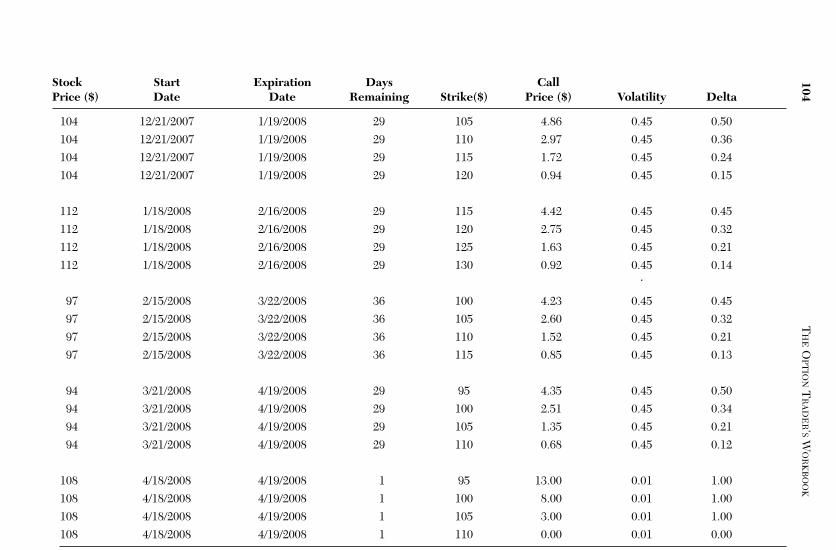
ptg
Stock Start Expiration Days CallPrice ($) Date Date Remaining Strike($) Price ($) Volatility Delta
104 12/21/2007 1/19/2008 29 105 4.86 0.45 0.50104 12/21/2007 1/19/2008 29 110 2.97 0.45 0.36104 12/21/2007 1/19/2008 29 115 1.72 0.45 0.24104 12/21/2007 1/19/2008 29 120 0.94 0.45 0.15
112 1/18/2008 2/16/2008 29 115 4.42 0.45 0.45112 1/18/2008 2/16/2008 29 120 2.75 0.45 0.32112 1/18/2008 2/16/2008 29 125 1.63 0.45 0.21112 1/18/2008 2/16/2008 29 130 0.92 0.45 0.14
‘97 2/15/2008 3/22/2008 36 100 4.23 0.45 0.4597 2/15/2008 3/22/2008 36 105 2.60 0.45 0.3297 2/15/2008 3/22/2008 36 110 1.52 0.45 0.2197 2/15/2008 3/22/2008 36 115 0.85 0.45 0.13
94 3/21/2008 4/19/2008 29 95 4.35 0.45 0.5094 3/21/2008 4/19/2008 29 100 2.51 0.45 0.3494 3/21/2008 4/19/2008 29 105 1.35 0.45 0.2194 3/21/2008 4/19/2008 29 110 0.68 0.45 0.12
108 4/18/2008 4/19/2008 1 95 13.00 0.01 1.00108 4/18/2008 4/19/2008 1 100 8.00 0.01 1.00108 4/18/2008 4/19/2008 1 105 3.00 0.01 1.00108 4/18/2008 4/19/2008 1 110 0.00 0.01 0.00
104T
HE
OPT
ION
TR
AD
ER’S
WO
RK
BO
OK
From the Library of Melissa Wong
ptg
14. For the timeframe beginning on 12/21 and ending on 4/19,which trade sequence generates the larger return? In percent-age terms, what is the overall profit for this trade?
Purchase 1,000 shares of stock on 12/21 and sell on 4/18.
or
Purchase 1,000 shares of stock and, for each expiration, sell 10contracts at the first strike that is at least $5 out-of-the-money.As mentioned earlier, each option trade should be settled, andthe next batch of calls sold, on an expiration Friday (12/21, 1/18,2/15, 3/21). All trades are finally settled at the market close on4/18.
Answer: The stock position alone returns $4,000 while the cov-ered call sequence returns $4,830. The following table outlinesthe gain or loss of the short call position at each expiration.
Initial Expiration Gain/Expiration Stock Stock Initial Final Loss Date Price ($) Price ($) Strike ($) Call ($) Call ($) ($)
1/19/2008 104 112 110 2.97 2.00 0.97
2/16/2008 112 97 120 2.75 0.00 2.75
3/22/2008 97 94 105 2.60 0.00 2.60
4/19/2008 94 108 100 2.51 8.00 –5.49
Total 0.83
The first three expirations return a profit of $6.32 but the finalexpiration loses $5.49, for a total short call return of only $0.83($830). Adding together the stock and short call profits yields anet return of $4,830. Since the total cost of the trade was 1,000shares of long stock at $104, the percent gain is $4,830 /$104,000 = 4.64%.
CHAPTER 3 • COVERED PUTS AND CALLS 105
From the Library of Melissa Wong
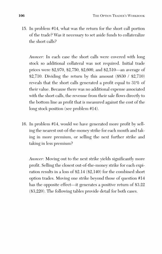
ptg
15. In problem #14, what was the return for the short call portionof the trade? Was it necessary to set aside funds to collateralizethe short calls?
Answer: In each case the short calls were covered with longstock so additional collateral was not required. Initial tradeprices were $2,970, $2,750, $2,600, and $2,510—an average of$2,710. Dividing the return by this amount ($830 / $2,710)reveals that the short calls generated a profit equal to 31% oftheir value. Because there was no additional expense associatedwith the short calls, the revenue from their sale flows directly tothe bottom line as profit that is measured against the cost of thelong stock position (see problem #14).
16. In problem #14, would we have generated more profit by sell-ing the nearest out-of-the-money strike for each month and tak-ing in more premium, or selling the next further strike andtaking in less premium?
Answer: Moving out to the next strike yields significantly moreprofit. Selling the closest out-of-the-money strike for each expi-ration results in a loss of $2.14 ($2,140) for the combined shortoption trades. Moving one strike beyond those of question #14has the opposite effect—it generates a positive return of $3.22($3,220). The following tables provide detail for both cases.
106 THE OPTION TRADER’S WORKBOOK
From the Library of Melissa Wong
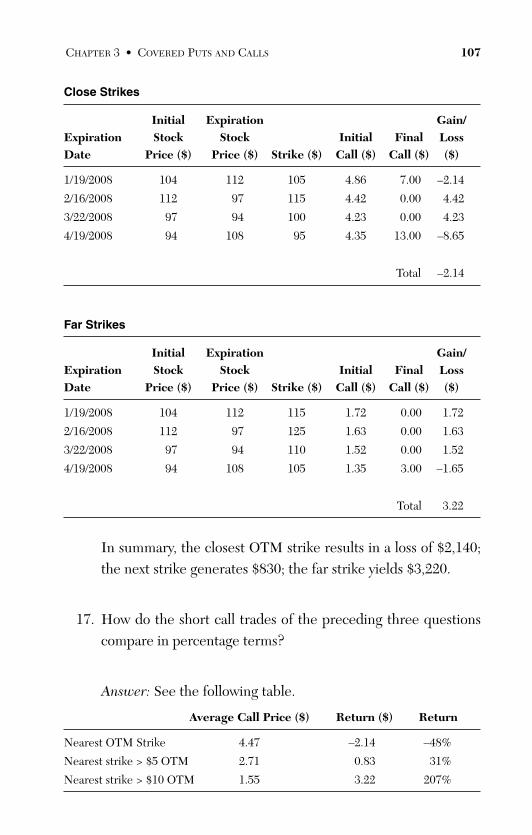
ptg
Close Strikes
Initial Expiration Gain/Expiration Stock Stock Initial Final Loss Date Price ($) Price ($) Strike ($) Call ($) Call ($) ($)
1/19/2008 104 112 105 4.86 7.00 –2.14
2/16/2008 112 97 115 4.42 0.00 4.42
3/22/2008 97 94 100 4.23 0.00 4.23
4/19/2008 94 108 95 4.35 13.00 –8.65
Total –2.14
Far Strikes
Initial Expiration Gain/Expiration Stock Stock Initial Final Loss Date Price ($) Price ($) Strike ($) Call ($) Call ($) ($)
1/19/2008 104 112 115 1.72 0.00 1.72
2/16/2008 112 97 125 1.63 0.00 1.63
3/22/2008 97 94 110 1.52 0.00 1.52
4/19/2008 94 108 105 1.35 3.00 –1.65
Total 3.22
In summary, the closest OTM strike results in a loss of $2,140;the next strike generates $830; the far strike yields $3,220.
17. How do the short call trades of the preceding three questionscompare in percentage terms?
Answer: See the following table.
Average Call Price ($) Return ($) Return
Nearest OTM Strike 4.47 –2.14 –48%
Nearest strike > $5 OTM 2.71 0.83 31%
Nearest strike > $10 OTM 1.55 3.22 207%
CHAPTER 3 • COVERED PUTS AND CALLS 107
From the Library of Melissa Wong
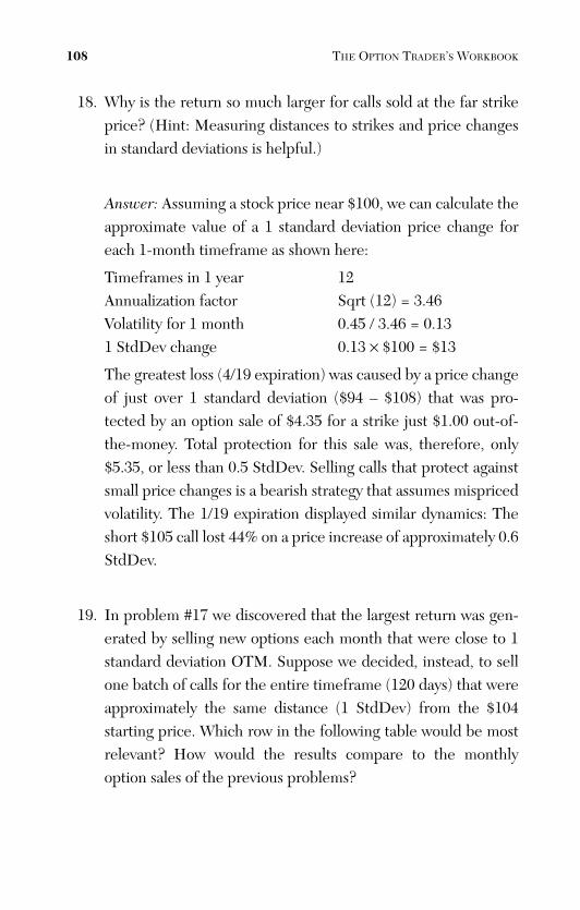
ptg
18. Why is the return so much larger for calls sold at the far strikeprice? (Hint: Measuring distances to strikes and price changesin standard deviations is helpful.)
Answer: Assuming a stock price near $100, we can calculate theapproximate value of a 1 standard deviation price change foreach 1-month timeframe as shown here:
Timeframes in 1 year 12Annualization factor Sqrt (12) = 3.46Volatility for 1 month 0.45 / 3.46 = 0.131 StdDev change 0.13 × $100 = $13
The greatest loss (4/19 expiration) was caused by a price changeof just over 1 standard deviation ($94 – $108) that was pro-tected by an option sale of $4.35 for a strike just $1.00 out-of-the-money. Total protection for this sale was, therefore, only$5.35, or less than 0.5 StdDev. Selling calls that protect againstsmall price changes is a bearish strategy that assumes mispricedvolatility. The 1/19 expiration displayed similar dynamics: Theshort $105 call lost 44% on a price increase of approximately 0.6StdDev.
19. In problem #17 we discovered that the largest return was gen-erated by selling new options each month that were close to 1standard deviation OTM. Suppose we decided, instead, to sellone batch of calls for the entire timeframe (120 days) that wereapproximately the same distance (1 StdDev) from the $104starting price. Which row in the following table would be mostrelevant? How would the results compare to the monthlyoption sales of the previous problems?
108 THE OPTION TRADER’S WORKBOOK
From the Library of Melissa Wong
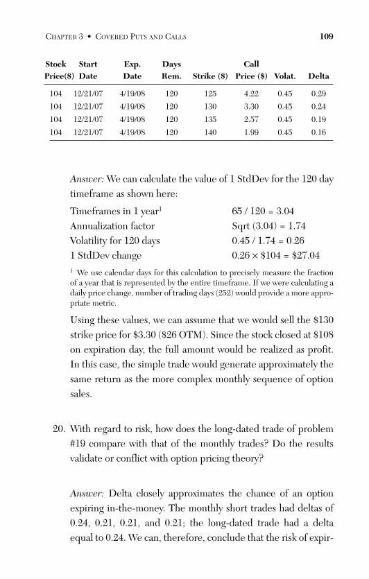
ptg
Stock Start Exp. Days CallPrice($) Date Date Rem. Strike ($) Price ($) Volat. Delta
104 12/21/07 4/19/08 120 125 4.22 0.45 0.29
104 12/21/07 4/19/08 120 130 3.30 0.45 0.24
104 12/21/07 4/19/08 120 135 2.57 0.45 0.19
104 12/21/07 4/19/08 120 140 1.99 0.45 0.16
Answer: We can calculate the value of 1 StdDev for the 120 daytimeframe as shown here:
Timeframes in 1 year1 65 / 120 = 3.04Annualization factor Sqrt (3.04) = 1.74Volatility for 120 days 0.45 / 1.74 = 0.261 StdDev change 0.26 × $104 = $27.041 We use calendar days for this calculation to precisely measure the fractionof a year that is represented by the entire timeframe. If we were calculating adaily price change, number of trading days (252) would provide a more appro-priate metric.
Using these values, we can assume that we would sell the $130strike price for $3.30 ($26 OTM). Since the stock closed at $108on expiration day, the full amount would be realized as profit.In this case, the simple trade would generate approximately thesame return as the more complex monthly sequence of optionsales.
20. With regard to risk, how does the long-dated trade of problem#19 compare with that of the monthly trades? Do the resultsvalidate or conflict with option pricing theory?
Answer: Delta closely approximates the chance of an optionexpiring in-the-money. The monthly short trades had deltas of0.24, 0.21, 0.21, and 0.21; the long-dated trade had a deltaequal to 0.24. We can, therefore, conclude that the risk of expir-
CHAPTER 3 • COVERED PUTS AND CALLS 109
From the Library of Melissa Wong
ptg
ing in-the-money was approximately equal for monthly andlong-dated short calls. These dynamics make sense becausemonthly and long-dated strike choices were both based on a 1standard deviation price change.
The results are a strong validation of option pricing theorybecause equal risks yielded comparable profits regardless of thetimeframe. Selling more expensive closer strikes was not a goodstrategy because potentially larger profits were offset by greaterrisks that occasionally materialized into substantial losses.
Option traders frequently make the mistake of selling seem-ingly expensive near-dated options that exhibit high levels oftime decay. This approach is flawed because correctly pricedoptions have balanced risk:reward profiles regardless of thetimeframe. However, monthly short sales can provide an advan-tage in rising volatility environments—bear markets being themost notable case. The following problems are designed withthis concept in mind.
In this section we will explore scenarios that involve a series ofcovered puts spanning four months. The following table con-tains relevant pricing information. As before, each section’sstart date corresponds to expiration Friday of the previous sec-tion. The sequence begins at December expiration with thestock trading at $106, and ends at April expiration with thestock at $66.
110 THE OPTION TRADER’S WORKBOOK
From the Library of Melissa Wong
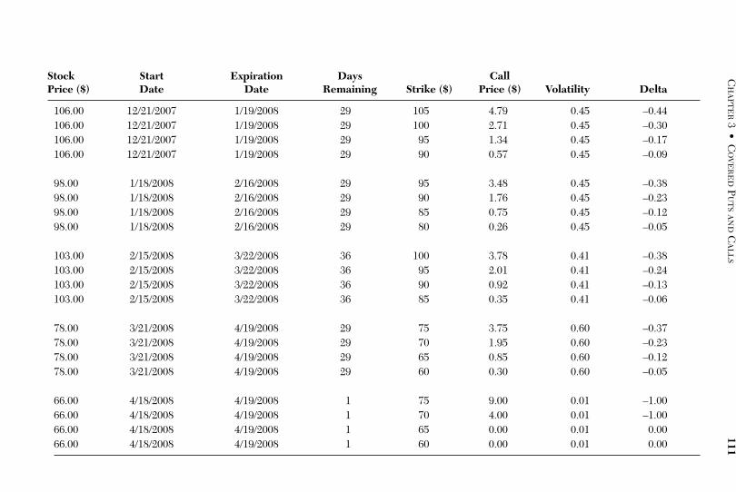
ptg
Stock Start Expiration Days CallPrice ($) Date Date Remaining Strike ($) Price ($) Volatility Delta
106.00 12/21/2007 1/19/2008 29 105 4.79 0.45 –0.44106.00 12/21/2007 1/19/2008 29 100 2.71 0.45 –0.30106.00 12/21/2007 1/19/2008 29 95 1.34 0.45 –0.17106.00 12/21/2007 1/19/2008 29 90 0.57 0.45 –0.09
98.00 1/18/2008 2/16/2008 29 95 3.48 0.45 –0.3898.00 1/18/2008 2/16/2008 29 90 1.76 0.45 –0.2398.00 1/18/2008 2/16/2008 29 85 0.75 0.45 –0.1298.00 1/18/2008 2/16/2008 29 80 0.26 0.45 –0.05
103.00 2/15/2008 3/22/2008 36 100 3.78 0.41 –0.38103.00 2/15/2008 3/22/2008 36 95 2.01 0.41 –0.24103.00 2/15/2008 3/22/2008 36 90 0.92 0.41 –0.13103.00 2/15/2008 3/22/2008 36 85 0.35 0.41 –0.06
78.00 3/21/2008 4/19/2008 29 75 3.75 0.60 –0.3778.00 3/21/2008 4/19/2008 29 70 1.95 0.60 –0.2378.00 3/21/2008 4/19/2008 29 65 0.85 0.60 –0.1278.00 3/21/2008 4/19/2008 29 60 0.30 0.60 –0.05
66.00 4/18/2008 4/19/2008 1 75 9.00 0.01 –1.0066.00 4/18/2008 4/19/2008 1 70 4.00 0.01 –1.0066.00 4/18/2008 4/19/2008 1 65 0.00 0.01 0.0066.00 4/18/2008 4/19/2008 1 60 0.00 0.01 0.00
CH
APT
ER
3•
CO
VE
RE
DP
UT
SA
ND
CA
LL
S111
From the Library of Melissa Wong
ptg
21. For the timeframe beginning on 12/21 and ending on 4/19,which trade sequence generates the larger return?
Short 1,000 shares of stock on 12/21 and close the trade on4/18.
or
Short 1,000 shares of stock and, for each expiration, sell 10 putsat the first strike that is at least $5 out-of-the-money. As men-tioned earlier, each option trade should be settled, and the nextbatch of puts sold, on an expiration Friday (12/21, 1/18, 2/15,3/21). All trades are finally settled at the market close on 4/18.
Answer: The stock position returns $40,000 while the coveredput sequence subtracts $14,570. The net result is a profit of$25,430. The following table outlines the gain or loss of theshort put position at each expiration.
Initial Expiration Gain/Expiration Stock Stock Initial Final Loss Date Price ($) Price ($) Strike ($) Put ($) Put ($) ($)
1/19/2008 106 98 100 2.71 2.00 0.71
2/16/2008 98 103 90 1.76 0.00 1.76
3/22/2008 103 78 95 2.01 17.00 –14.99
4/19/2008 78 66 70 1.95 4.00 –2.05
Total –14.57
22. When a company reports very negative financial news thatshocks the market, the resulting stock drawdown is normallyaccompanied by a sharp increase in implied volatility. Spikes of300%, 400%, and even 500% are not uncommon in thesesituations.
112 THE OPTION TRADER’S WORKBOOK
From the Library of Melissa Wong
ptg
Consider a covered put position that is short 1,000 shares ofstock at $107 and 10 puts at the $105 strike as outlined in thefollowing table. Line 1 of the table displays the starting putposition, and line 2 reveals the results after a severe downwardprice spike accompanied by a large increase in implied volatilityfrom 30% to 170%.
Stock Days Put Price ($) Rem. Strike($) Price ($) Volat. Delta Theta
107 29 105 2.61 0.30 –0.39 –0.06
80 25 105 31.61 1.70 –0.65 –0.26
How much money has the trade lost? Assuming that bothimplied volatility and stock price remain constant, how manydays must elapse before the trade reaches a break-even point?How much will the trade recover if the stock closes at $80 onexpiration day? What will the final profit be?
Answer: With 25 days remaining before expiration, the tradehas lost $2 ($27 gain on short stock offset by $29 loss on shortputs).
With a theta of –$0.26, approximately 8 days must elapse torecover the $2 loss ($0.26 × 8 = 2.08).
If the stock closes the expiration timeframe at $80, the tradewill be worth $6.37 calculated as shown here:
Profit from short stock $27.00Sale of short put $2.61Cost to repurchase short put –$25.00Trade profit $4.61
The final profit realized at expiration is a $2.61 improvementover the $2.00 loss experienced after the large downward spikedisplayed in the table. Overall, the combined stock and optiontrades generated a profit of $4,610.
CHAPTER 3 • COVERED PUTS AND CALLS 113
From the Library of Melissa Wong
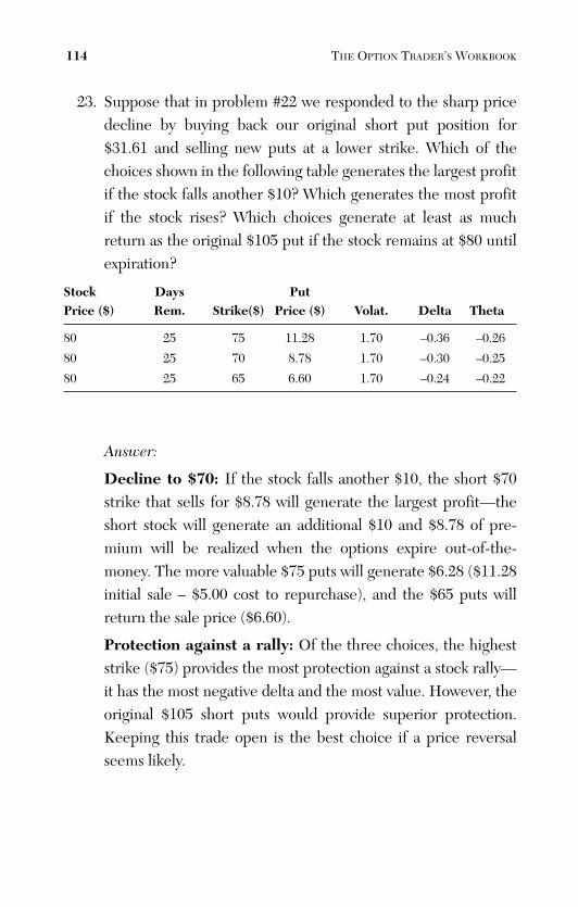
ptg
23. Suppose that in problem #22 we responded to the sharp pricedecline by buying back our original short put position for$31.61 and selling new puts at a lower strike. Which of thechoices shown in the following table generates the largest profitif the stock falls another $10? Which generates the most profitif the stock rises? Which choices generate at least as muchreturn as the original $105 put if the stock remains at $80 untilexpiration?
Stock Days Put Price ($) Rem. Strike($) Price ($) Volat. Delta Theta
80 25 75 11.28 1.70 –0.36 –0.26
80 25 70 8.78 1.70 –0.30 –0.25
80 25 65 6.60 1.70 –0.24 –0.22
Answer:
Decline to $70: If the stock falls another $10, the short $70strike that sells for $8.78 will generate the largest profit—theshort stock will generate an additional $10 and $8.78 of pre-mium will be realized when the options expire out-of-the-money. The more valuable $75 puts will generate $6.28 ($11.28initial sale – $5.00 cost to repurchase), and the $65 puts willreturn the sale price ($6.60).
Protection against a rally: Of the three choices, the higheststrike ($75) provides the most protection against a stock rally—it has the most negative delta and the most value. However, theoriginal $105 short puts would provide superior protection.Keeping this trade open is the best choice if a price reversalseems likely.
114 THE OPTION TRADER’S WORKBOOK
From the Library of Melissa Wong
ptg
Stock remains at $80: At the time of the downward spike, theoriginal $105 puts were $25 in-the-money but traded for$31.61. Subtracting intrinsic from actual value ($31.61 –$25.00) reveals that the contracts had $6.61 of remaining timepremium that must decay away before expiration. We can usethis number for comparison against the three new choices,which each return their full sale price at expiration as theyexpire out-of-the-money. The first two choices yield higherreturns than the original trade ($11.28 and $8.78). The thirdchoice provides approximately the same return ($6.60).
Pure Option Covered Positions(Problems #24–#28)
The following section focuses on covered positions composed ofequal numbers of long and short options in which the long side hasmore favorable terms (same or later expiration and same or closerstrike). Many investors who trade covered positions favor thisapproach because it requires less capital, limits downside exposure,and benefits from leverage.
The following two tables display relevant pricing information forthe problems that follow. The first table is organized by month andstrike price. As before, each section’s start date corresponds to expira-tion Friday of the previous group. The sequence begins at Decemberexpiration with the stock trading at $104, and ends at April expirationwith the stock at $133.
The second table is composed of a single set of entries that spanthe entire timeframe. It provides long-dated option prices that com-plement those of the previous table.
CHAPTER 3 • COVERED PUTS AND CALLS 115
From the Library of Melissa Wong
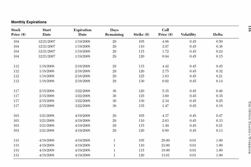
ptg
Monthly Expirations
Stock Start Expiration Days CallPrice ($) Date Date Remaining Strike ($) Price ($) Volatility Delta
104 12/21/2007 1/19/2008 29 105 4.86 0.45 0.50104 12/21/2007 1/19/2008 29 110 2.97 0.45 0.36104 12/21/2007 1/19/2008 29 115 1.72 0.45 0.24104 12/21/2007 1/19/2008 29 120 0.94 0.45 0.15
112 1/18/2008 2/16/2008 29 115 4.42 0.45 0.45112 1/18/2008 2/16/2008 29 120 2.75 0.45 0.32112 1/18/2008 2/16/2008 29 125 1.63 0.45 0.21112 1/18/2008 2/16/2008 29 130 0.92 0.45 0.14
117 2/15/2008 3/22/2008 36 120 5.35 0.45 0.46117 2/15/2008 3/22/2008 36 125 3.60 0.45 0.35117 2/15/2008 3/22/2008 36 130 2.34 0.45 0.25117 2/15/2008 3/22/2008 36 135 1.47 0.45 0.18
103 3/21/2008 4/19/2008 29 105 4.37 0.45 0.47103 3/21/2008 4/19/2008 29 110 2.63 0.45 0.33103 3/21/2008 4/19/2008 29 115 1.49 0.45 0.21103 3/21/2008 4/19/2008 29 120 0.80 0.45 0.13
133 4/18/2008 4/19/2008 1 105 28.00 0.01 1.00133 4/18/2008 4/19/2008 1 110 23.00 0.01 1.00133 4/18/2008 4/19/2008 1 115 18.00 0.01 1.00133 4/18/2008 4/19/2008 1 120 13.01 0.01 1.00
116T
HE
OPT
ION
TR
AD
ER’S
WO
RK
BO
OK
From the Library of Melissa Wong
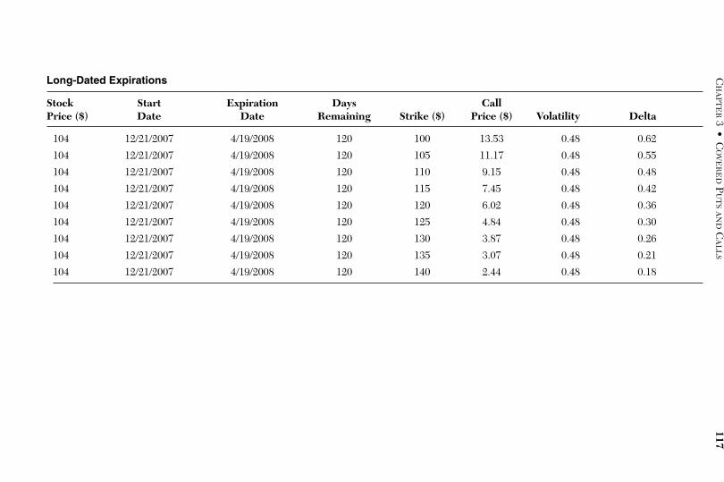
ptg
Long-Dated Expirations
Stock Start Expiration Days CallPrice ($) Date Date Remaining Strike ($) Price ($) Volatility Delta
104 12/21/2007 4/19/2008 120 100 13.53 0.48 0.62
104 12/21/2007 4/19/2008 120 105 11.17 0.48 0.55
104 12/21/2007 4/19/2008 120 110 9.15 0.48 0.48
104 12/21/2007 4/19/2008 120 115 7.45 0.48 0.42
104 12/21/2007 4/19/2008 120 120 6.02 0.48 0.36
104 12/21/2007 4/19/2008 120 125 4.84 0.48 0.30
104 12/21/2007 4/19/2008 120 130 3.87 0.48 0.26
104 12/21/2007 4/19/2008 120 135 3.07 0.48 0.21
104 12/21/2007 4/19/2008 120 140 2.44 0.48 0.18
CH
APT
ER
3•
CO
VE
RE
DP
UT
SA
ND
CA
LL
S117
From the Library of Melissa Wong
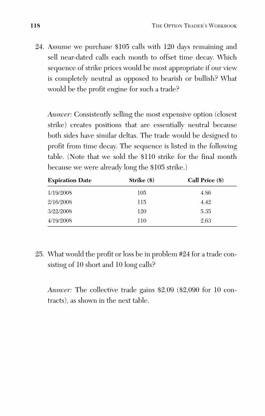
ptg
24. Assume we purchase $105 calls with 120 days remaining andsell near-dated calls each month to offset time decay. Whichsequence of strike prices would be most appropriate if our viewis completely neutral as opposed to bearish or bullish? Whatwould be the profit engine for such a trade?
Answer: Consistently selling the most expensive option (closeststrike) creates positions that are essentially neutral becauseboth sides have similar deltas. The trade would be designed toprofit from time decay. The sequence is listed in the followingtable. (Note that we sold the $110 strike for the final monthbecause we were already long the $105 strike.)
Expiration Date Strike ($) Call Price ($)
1/19/2008 105 4.86
2/16/2008 115 4.42
3/22/2008 120 5.35
4/19/2008 110 2.63
25. What would the profit or loss be in problem #24 for a trade con-sisting of 10 short and 10 long calls?
Answer: The collective trade gains $2.09 ($2,090 for 10 con-tracts), as shown in the next table.
118 THE OPTION TRADER’S WORKBOOK
From the Library of Melissa Wong
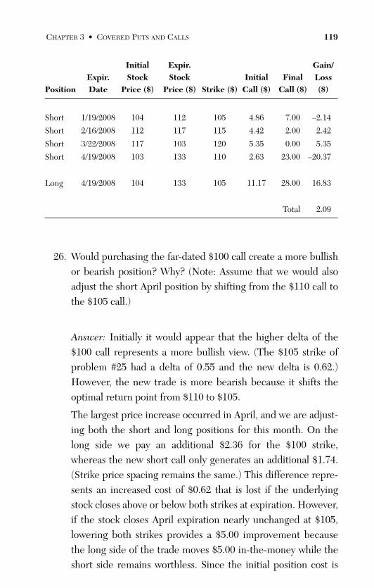
ptg
Initial Expir. Gain/Expir. Stock Stock Initial Final Loss
Position Date Price ($) Price ($) Strike ($) Call ($) Call ($) ($)
Short 1/19/2008 104 112 105 4.86 7.00 –2.14
Short 2/16/2008 112 117 115 4.42 2.00 2.42
Short 3/22/2008 117 103 120 5.35 0.00 5.35
Short 4/19/2008 103 133 110 2.63 23.00 –20.37
Long 4/19/2008 104 133 105 11.17 28.00 16.83
Total 2.09
26. Would purchasing the far-dated $100 call create a more bullishor bearish position? Why? (Note: Assume that we would alsoadjust the short April position by shifting from the $110 call tothe $105 call.)
Answer: Initially it would appear that the higher delta of the$100 call represents a more bullish view. (The $105 strike ofproblem #25 had a delta of 0.55 and the new delta is 0.62.)However, the new trade is more bearish because it shifts theoptimal return point from $110 to $105.
The largest price increase occurred in April, and we are adjust-ing both the short and long positions for this month. On thelong side we pay an additional $2.36 for the $100 strike,whereas the new short call only generates an additional $1.74.(Strike price spacing remains the same.) This difference repre-sents an increased cost of $0.62 that is lost if the underlyingstock closes above or below both strikes at expiration. However,if the stock closes April expiration nearly unchanged at $105,lowering both strikes provides a $5.00 improvement becausethe long side of the trade moves $5.00 in-the-money while theshort side remains worthless. Since the initial position cost is
CHAPTER 3 • COVERED PUTS AND CALLS 119
From the Library of Melissa Wong
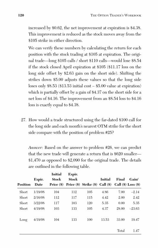
ptg
increased by $0.62, the net improvement at expiration is $4.38.This improvement is reduced as the stock moves away from the$105 strike in either direction.
We can verify these numbers by calculating the return for eachposition with the stock trading at $105 at expiration. The origi-nal trade—long $105 calls / short $110 calls—would lose $8.54if the stock closed April expiration at $105 ($11.17 loss on thelong side offset by $2.63 gain on the short side). Shifting thestrikes down $5.00 adjusts these values so that the long sideloses only $8.53 ($13.53 initial cost – $5.00 value at expiration)which is partially offset by a gain of $4.37 on the short side for anet loss of $4.16. The improvement from an $8.54 loss to $4.16loss is exactly equal to $4.38.
27. How would a trade structured using the far-dated $100 call forthe long side and each month’s nearest OTM strike for the shortside compare with the position of problem #25?
Answer: Based on the answer to problem #26, we can predictthat the new trade will generate a return that is $620 smaller—$1,470 as opposed to $2,090 for the original trade. The detailsare outlined in the following table.
Initial Expir.Expir. Stock Stock Initial Final Gain/
Position Date Price ($) Price ($) Strike ($) Call ($) Call ($) Loss ($)
Short 1/19/08 104 112 105 4.86 7.00 –2.14
Short 2/16/08 112 117 115 4.42 2.00 2.42
Short 3/22/08 117 103 120 5.35 0.00 5.35
Short 4/19/08 103 133 105 4.37 28.00 –23.63
Long 4/19/08 104 133 100 13.53 33.00 19.47
Total 1.47
120 THE OPTION TRADER’S WORKBOOK
From the Library of Melissa Wong
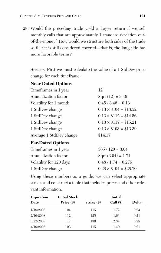
ptg
28. Would the preceding trade yield a larger return if we sellmonthly calls that are approximately 1 standard deviation out-of-the-money? How would we structure both sides of the tradeso that it is still considered covered—that is, the long side hasmore favorable terms?
Answer: First we must calculate the value of a 1 StdDev pricechange for each timeframe.
Near-Dated OptionsTimeframes in 1 year 12Annualization factor Sqrt (12) = 3.46Volatility for 1 month 0.45 / 3.46 = 0.131 StdDev change 0.13 × $104 = $13.521 StdDev change 0.13 × $112 = $14.561 StdDev change 0.13 × $117 = $15.211 StdDev change 0.13 × $103 = $13.39Average 1 StdDev change $14.17
Far-Dated OptionsTimeframes in 1 year 365 / 120 = 3.04Annualization factor Sqrt (3.04) = 1.74Volatility for 120 days 0.48 / 1.74 = 0.2761 StdDev change 0.28 × $104 = $28.70
Using these numbers as a guide, we can select appropriatestrikes and construct a table that includes prices and other rele-vant information.
Expiration Initial Stock Initial Date Price ($) Strike ($) Call ($) Delta
1/19/2008 104 115 1.72 0.24
2/16/2008 112 125 1.63 0.21
3/22/2008 117 130 2.34 0.25
4/19/2008 103 115 1.49 0.21
CHAPTER 3 • COVERED PUTS AND CALLS 121
From the Library of Melissa Wong
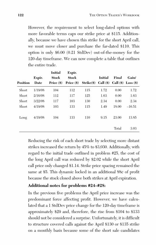
ptg
However, the requirement to select long-dated options withmore favorable terms caps our strike price at $115. Addition-ally, because we have chosen this strike for the short April call,we must move closer and purchase the far-dated $110. Thisoption is only $6.00 (0.21 StdDev) out-of-the-money for the120-day timeframe. We can now complete a table that outlinesthe entire trade.
Initial Expir.Expir. Stock Stock Initial Final Gain/
Position Date Price ($) Price ($) Strike($) Call ($) Call ($) Loss ($)
Short 1/19/08 104 112 115 1.72 0.00 1.72
Short 2/16/08 112 117 125 1.63 0.00 1.63
Short 3/22/08 117 103 130 2.34 0.00 2.34
Short 4/19/08 103 133 115 1.49 18.00 –16.51
Long 4/19/08 104 133 110 9.15 23.00 13.85
Total 3.03
Reducing the risk of each short trade by selecting more distantstrikes increased the return by 45% to $3,030. Additionally, withregard to the initial trade outlined in problem #25, the cost ofthe long April call was reduced by $2.02 while the short Aprilcall price only changed $1.14. Strike price spacing remained thesame at $5. This dynamic locked in an additional 88¢ of profitbecause the stock closed above both strikes at April expiration.
Additional notes for problems #24–#28:
In the previous five problems the April price increase was thepredominant force affecting profit. However, we have calcu-lated that a 1 StdDev price change for the 120-day timeframe isapproximately $29 and, therefore, the rise from $104 to $133should not be considered a surprise. Unfortunately, it is difficultto structure covered calls against the April $130 or $135 strikeon a monthly basis because some of the short sale candidates
122 THE OPTION TRADER’S WORKBOOK
From the Library of Melissa Wong
ptg
have virtually no value. More specifically, both the January andthe April $135 calls would be worth only 10¢ at the time of sale.Generally speaking, it is more reasonable to allow short-termrisk parameters for each short option sale to drive strike priceselection.
Summary
Our discussion began with traditional covered calls that are struc-tured with long stock and an equivalent number of short calls. As wehave seen, the dynamics of position management change dramaticallywhen long calls are substituted for long stock or long puts replaceshort stock, because stock always has a delta of 1.00 and options obvi-ously do not.
The present discussion focused on covered trades in which theshort side has less favorable terms and potential losses are somewhatlimited. The next section will expand this discussion to include tradestructures in which the time decay of a far-dated long position is offsetby near-dated options with a more favorable strike price. Such trades,because they are uncovered, require a more sophisticated approach torisk management.
Finally, we will build on these dynamics with more complex struc-tures that involve ratios where the two sides—long and short—con-tain different numbers of contracts. These trades can take manydifferent forms, including some that are quite complex. All variationsinclude uncovered short components. Risk management will play anincreasingly important role as the complexity increases. Generallyspeaking, not losing money is the most efficient way for an optiontrader to generate a profit.
CHAPTER 3 • COVERED PUTS AND CALLS 123
From the Library of Melissa Wong

ptg
This page intentionally left blank
From the Library of Melissa Wong
ptg
Complex Trades—Part 1
The preceding chapter focused on covered trades that limit thepotential loss of a short option position. Covered trades also providedownside protection for the complementary long position. However,this downside protection is limited to the value of the short option,and that value is realized only at expiration. These dynamics can beproblematic for stock investors seeking more balanced positions in anunstable market.
Option traders generally solve this problem by structuring pureoption positions that do not involve stock. Rather than purchasing1,000 shares of stock and sell a call that is worth $2.50, an optiontrader might choose to purchase a $5.00 call and sell a $2.50 call at amore distant strike price. In this case, the total risk is limited to $2.50regardless of how far the stock falls. As we saw in the preceding chap-ter, this simple vertical spread has a risk:return profile that is muchdifferent from a stock-based covered call.
A bearish investor might choose to take the other side of thistrade by selling the lower strike and purchasing the higher one. Thetrade would have a $2.50 credit and the potential loss, in the eventthat the stock rises, would be capped by the long option. Despite thecap, this trade is not considered covered because the short option hasa more favorable strike price. Collateral is required, but the cost isalso capped by the difference between the strikes. We will explorethe dynamics of this trade, also known as a bear spread, in the open-ing sections of this chapter.
4
125
From the Library of Melissa Wong
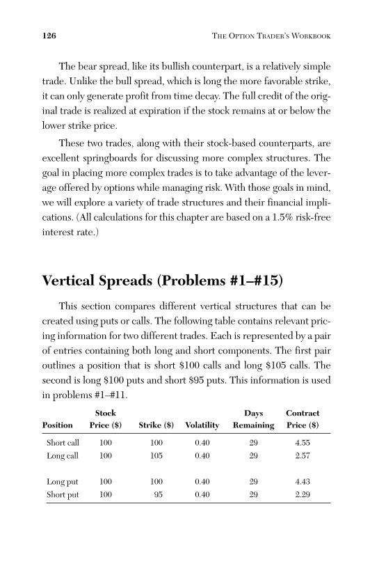
ptg
The bear spread, like its bullish counterpart, is a relatively simpletrade. Unlike the bull spread, which is long the more favorable strike,it can only generate profit from time decay. The full credit of the orig-inal trade is realized at expiration if the stock remains at or below thelower strike price.
These two trades, along with their stock-based counterparts, areexcellent springboards for discussing more complex structures. Thegoal in placing more complex trades is to take advantage of the lever-age offered by options while managing risk. With those goals in mind,we will explore a variety of trade structures and their financial impli-cations. (All calculations for this chapter are based on a 1.5% risk-freeinterest rate.)
Vertical Spreads (Problems #1–#15)
This section compares different vertical structures that can becreated using puts or calls. The following table contains relevant pric-ing information for two different trades. Each is represented by a pairof entries containing both long and short components. The first pairoutlines a position that is short $100 calls and long $105 calls. Thesecond is long $100 puts and short $95 puts. This information is usedin problems #1–#11.
Stock Days Contract Position Price ($) Strike ($) Volatility Remaining Price ($)
Short call 100 100 0.40 29 4.55
Long call 100 105 0.40 29 2.57
Long put 100 100 0.40 29 4.43
Short put 100 95 0.40 29 2.29
126 THE OPTION TRADER’S WORKBOOK
From the Library of Melissa Wong
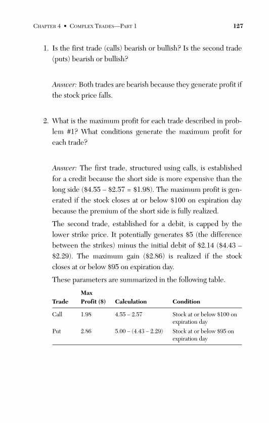
ptg
1. Is the first trade (calls) bearish or bullish? Is the second trade(puts) bearish or bullish?
Answer: Both trades are bearish because they generate profit ifthe stock price falls.
2. What is the maximum profit for each trade described in prob-lem #1? What conditions generate the maximum profit foreach trade?
Answer: The first trade, structured using calls, is establishedfor a credit because the short side is more expensive than thelong side ($4.55 – $2.57 = $1.98). The maximum profit is gen-erated if the stock closes at or below $100 on expiration daybecause the premium of the short side is fully realized.
The second trade, established for a debit, is capped by thelower strike price. It potentially generates $5 (the differencebetween the strikes) minus the initial debit of $2.14 ($4.43 –$2.29). The maximum gain ($2.86) is realized if the stockcloses at or below $95 on expiration day.
These parameters are summarized in the following table.
MaxTrade Profit ($) Calculation Condition
Call 1.98 4.55 – 2.57 Stock at or below $100 onexpiration day
Put 2.86 5.00 – (4.43 – 2.29) Stock at or below $95 onexpiration day
CHAPTER 4 • COMPLEX TRADES—PART 1 127
From the Library of Melissa Wong
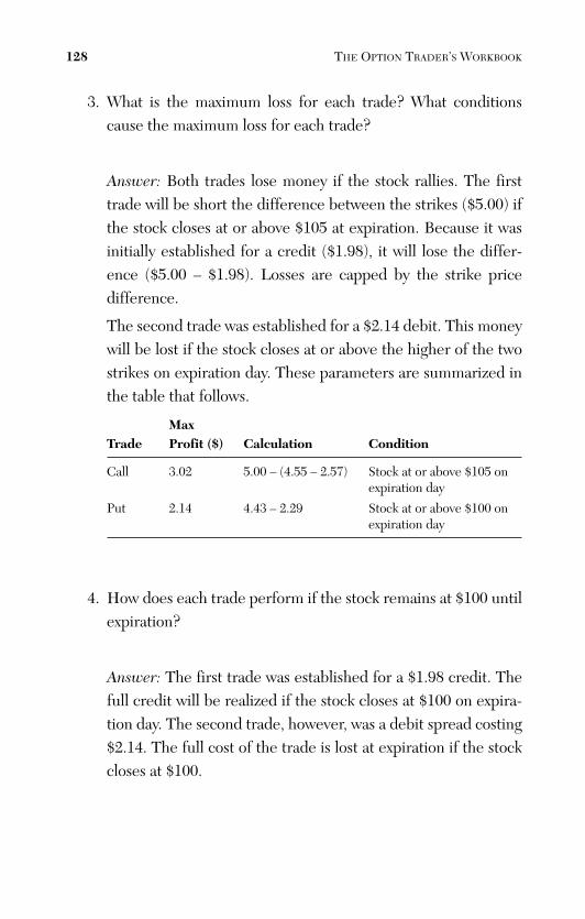
ptg
3. What is the maximum loss for each trade? What conditionscause the maximum loss for each trade?
Answer: Both trades lose money if the stock rallies. The firsttrade will be short the difference between the strikes ($5.00) ifthe stock closes at or above $105 at expiration. Because it wasinitially established for a credit ($1.98), it will lose the differ-ence ($5.00 – $1.98). Losses are capped by the strike pricedifference.
The second trade was established for a $2.14 debit. This moneywill be lost if the stock closes at or above the higher of the twostrikes on expiration day. These parameters are summarized inthe table that follows.
MaxTrade Profit ($) Calculation Condition
Call 3.02 5.00 – (4.55 – 2.57) Stock at or above $105 onexpiration day
Put 2.14 4.43 – 2.29 Stock at or above $100 onexpiration day
4. How does each trade perform if the stock remains at $100 untilexpiration?
Answer: The first trade was established for a $1.98 credit. Thefull credit will be realized if the stock closes at $100 on expira-tion day. The second trade, however, was a debit spread costing$2.14. The full cost of the trade is lost at expiration if the stockcloses at $100.
128 THE OPTION TRADER’S WORKBOOK
From the Library of Melissa Wong
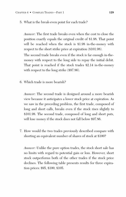
ptg
5. What is the break-even point for each trade?
Answer: The first trade breaks even when the cost to close theposition exactly equals the original credit of $1.98. That pointwill be reached when the stock is $1.98 in-the-money withrespect to the short strike price at expiration ($101.98).
The second trade breaks even if the stock is far enough in-the-money with respect to the long side to repay the initial debit.That point is reached if the stock trades $2.14 in-the-moneywith respect to the long strike ($97.86).
6. Which trade is more bearish?
Answer: The second trade is designed around a more bearishview because it anticipates a lower stock price at expiration. Aswe saw in the preceding problem, the first trade, composed oflong and short calls, breaks even if the stock rises slightly to$101.98. The second trade, composed of long and short puts,will lose money if the stock does not fall below $97.86.
7. How would the two trades previously described compare withshorting an equivalent number of shares of stock at $100?
Answer: Unlike the pure option trades, the stock short sale hasno limits with regard to potential gain or loss. However, shortstock outperforms both of the other trades if the stock pricedeclines. The following table presents results for three expira-tion prices: $95, $100, $105.
CHAPTER 4 • COMPLEX TRADES—PART 1 129
From the Library of Melissa Wong
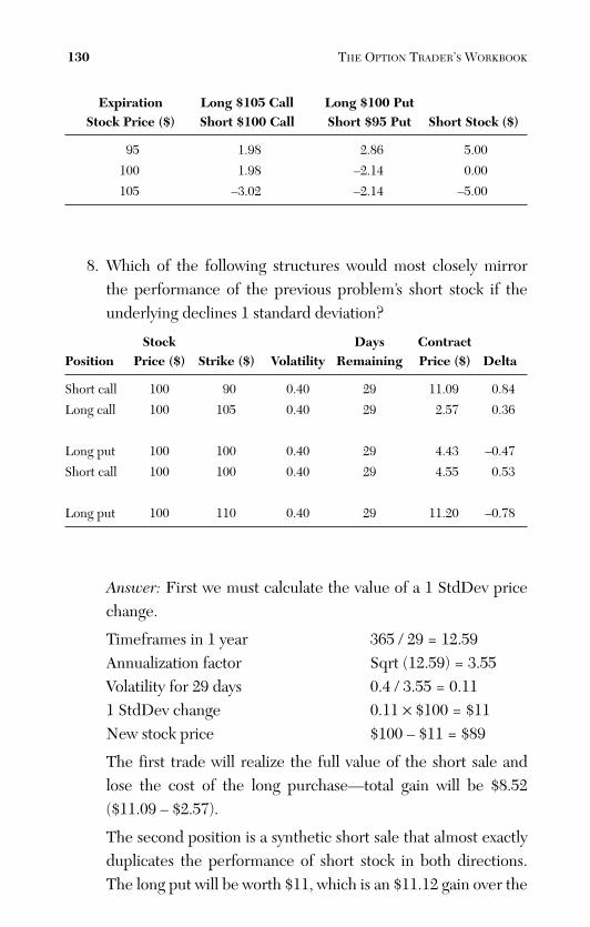
ptg
Expiration Long $105 Call Long $100 Put Stock Price ($) Short $100 Call Short $95 Put Short Stock ($)
95 1.98 2.86 5.00
100 1.98 –2.14 0.00
105 –3.02 –2.14 –5.00
8. Which of the following structures would most closely mirrorthe performance of the previous problem’s short stock if theunderlying declines 1 standard deviation?
Stock Days ContractPosition Price ($) Strike ($) Volatility Remaining Price ($) Delta
Short call 100 90 0.40 29 11.09 0.84
Long call 100 105 0.40 29 2.57 0.36
Long put 100 100 0.40 29 4.43 –0.47
Short call 100 100 0.40 29 4.55 0.53
Long put 100 110 0.40 29 11.20 –0.78
Answer: First we must calculate the value of a 1 StdDev pricechange.
Timeframes in 1 year 365 / 29 = 12.59Annualization factor Sqrt (12.59) = 3.55Volatility for 29 days 0.4 / 3.55 = 0.111 StdDev change 0.11 × $100 = $11New stock price $100 – $11 = $89
The first trade will realize the full value of the short sale andlose the cost of the long purchase—total gain will be $8.52($11.09 – $2.57).
The second position is a synthetic short sale that almost exactlyduplicates the performance of short stock in both directions.The long put will be worth $11, which is an $11.12 gain over the
130 THE OPTION TRADER’S WORKBOOK
From the Library of Melissa Wong
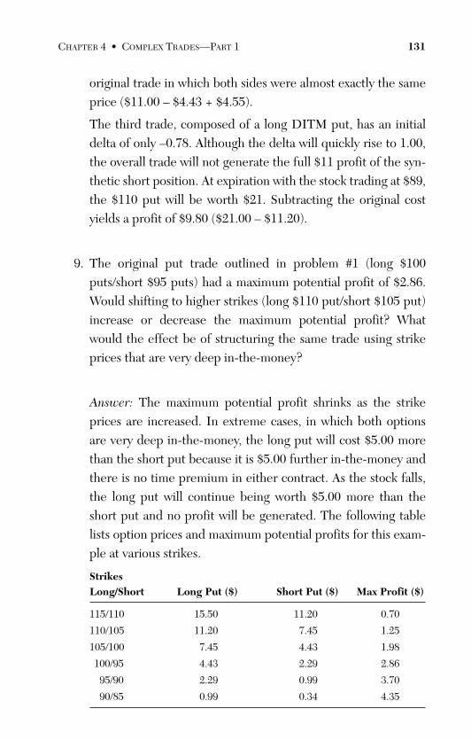
ptg
original trade in which both sides were almost exactly the sameprice ($11.00 – $4.43 + $4.55).
The third trade, composed of a long DITM put, has an initialdelta of only –0.78. Although the delta will quickly rise to 1.00,the overall trade will not generate the full $11 profit of the syn-thetic short position. At expiration with the stock trading at $89,the $110 put will be worth $21. Subtracting the original costyields a profit of $9.80 ($21.00 – $11.20).
9. The original put trade outlined in problem #1 (long $100puts/short $95 puts) had a maximum potential profit of $2.86.Would shifting to higher strikes (long $110 put/short $105 put)increase or decrease the maximum potential profit? Whatwould the effect be of structuring the same trade using strikeprices that are very deep in-the-money?
Answer: The maximum potential profit shrinks as the strikeprices are increased. In extreme cases, in which both optionsare very deep in-the-money, the long put will cost $5.00 morethan the short put because it is $5.00 further in-the-money andthere is no time premium in either contract. As the stock falls,the long put will continue being worth $5.00 more than theshort put and no profit will be generated. The following tablelists option prices and maximum potential profits for this exam-ple at various strikes.
StrikesLong/Short Long Put ($) Short Put ($) Max Profit ($)
115/110 15.50 11.20 0.70
110/105 11.20 7.45 1.25
105/100 7.45 4.43 1.98
100/95 4.43 2.29 2.86
95/90 2.29 0.99 3.70
90/85 0.99 0.34 4.35
CHAPTER 4 • COMPLEX TRADES—PART 1 131
From the Library of Melissa Wong
ptg
10. In problem #9 how does increasing the strike prices affect thedeltas of the two puts? How does the relative differencechange?
Answer: As the strike prices are raised, the deltas of both sideswill decrease, with the short delta decreasing faster than thelong delta. The values will continue to converge until they reach–1.00 and both sides are deep in-the-money. After this point isreached, the prices will differ by an amount equal to the spacebetween the strikes.
11. Suppose, as before, that we establish a trade that is long $100puts and short $95 puts. How will the maximum potential profitof our trade be affected if a sharp downward spike skews pricesso that options are priced with a relatively steep volatilitysmile—that is, implied volatility can be visualized on a con-stantly steepening curve that rises with lower strikes.
Answer: A steep volatility smile will disproportionately raise thevalue of the lower strike, the overall position will becomeshorter, and interim profit will shrink. However, the maximumpotential profit at expiration, with both options deep in-the-money, will remain the same because the higher strike will stillbe worth $5.00 more than the lower strike.
12. Problems #1–#10 assumed that implied volatility when thetrades were launched was 0.40 for all strikes. Suppose, however,
132 THE OPTION TRADER’S WORKBOOK
From the Library of Melissa Wong
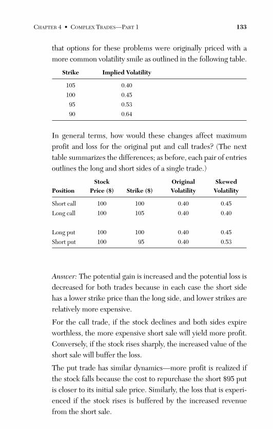
ptg
that options for these problems were originally priced with amore common volatility smile as outlined in the following table.
Strike Implied Volatility
105 0.40
100 0.45
95 0.53
90 0.64
In general terms, how would these changes affect maximumprofit and loss for the original put and call trades? (The nexttable summarizes the differences; as before, each pair of entriesoutlines the long and short sides of a single trade.)
Stock Original Skewed Position Price ($) Strike ($) Volatility Volatility
Short call 100 100 0.40 0.45
Long call 100 105 0.40 0.40
Long put 100 100 0.40 0.45
Short put 100 95 0.40 0.53
Answer: The potential gain is increased and the potential loss isdecreased for both trades because in each case the short sidehas a lower strike price than the long side, and lower strikes arerelatively more expensive.
For the call trade, if the stock declines and both sides expireworthless, the more expensive short sale will yield more profit.Conversely, if the stock rises sharply, the increased value of theshort sale will buffer the loss.
The put trade has similar dynamics—more profit is realized ifthe stock falls because the cost to repurchase the short $95 putis closer to its initial sale price. Similarly, the loss that is experi-enced if the stock rises is buffered by the increased revenuefrom the short sale.
CHAPTER 4 • COMPLEX TRADES—PART 1 133
From the Library of Melissa Wong
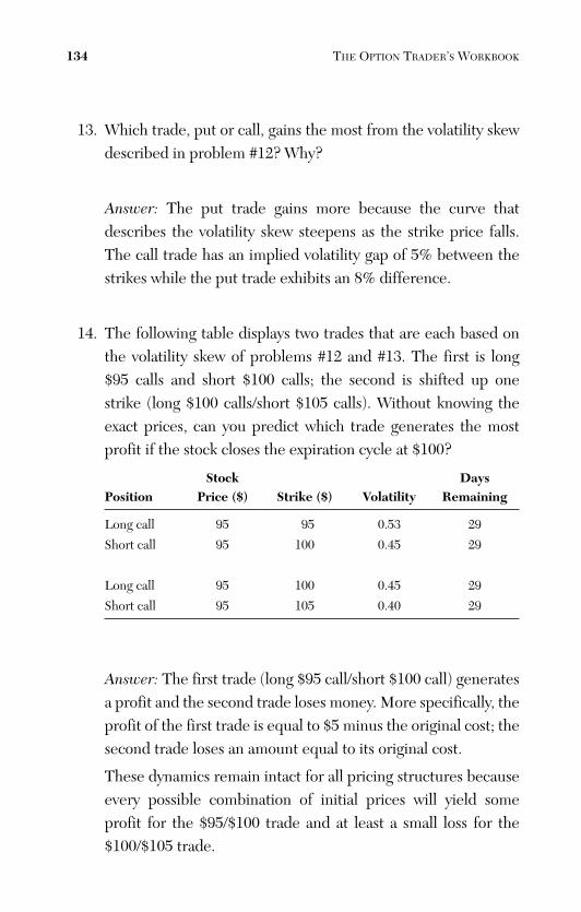
ptg
13. Which trade, put or call, gains the most from the volatility skewdescribed in problem #12? Why?
Answer: The put trade gains more because the curve thatdescribes the volatility skew steepens as the strike price falls.The call trade has an implied volatility gap of 5% between thestrikes while the put trade exhibits an 8% difference.
14. The following table displays two trades that are each based onthe volatility skew of problems #12 and #13. The first is long$95 calls and short $100 calls; the second is shifted up onestrike (long $100 calls/short $105 calls). Without knowing theexact prices, can you predict which trade generates the mostprofit if the stock closes the expiration cycle at $100?
Stock Days Position Price ($) Strike ($) Volatility Remaining
Long call 95 95 0.53 29
Short call 95 100 0.45 29
Long call 95 100 0.45 29
Short call 95 105 0.40 29
Answer: The first trade (long $95 call/short $100 call) generatesa profit and the second trade loses money. More specifically, theprofit of the first trade is equal to $5 minus the original cost; thesecond trade loses an amount equal to its original cost.
These dynamics remain intact for all pricing structures becauseevery possible combination of initial prices will yield someprofit for the $95/$100 trade and at least a small loss for the$100/$105 trade.
134 THE OPTION TRADER’S WORKBOOK
From the Library of Melissa Wong
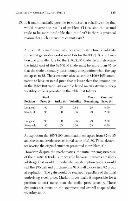
ptg
15. Is it mathematically possible to structure a volatility smile thatwould reverse the results of problem #14 causing the secondtrade to be more profitable than the first? Is there a practicalreason that such a structure cannot exist?
Answer: It is mathematically possible to structure a volatilitysmile that generates a substantial loss for the $95/$100 combina-tion and a smaller loss for the $100/$105 trade. In this structurethe initial cost of the $95/$100 trade must be more than $5 sothat the trade ultimately loses money at expiration when the gapcollapses to $5. The skew must also cause the $100/$105 combi-nation to have an initial price that is lower than the amount lostin the $95/$100 trade. An example based on an extremely steepvolatility smile is provided in the table that follows.
Stock Days Contract Position Price ($) Strike ($) Volatility Remaining Price ($)
Long call 95 95 0.84 29 9.00
Short call 95 100 0.36 29 2.00
Long call 95 100 0.36 29 2.00
Short call 95 105 0.30 29 0.50
At expiration the $95/$100 combination collapses from $7 to $5and the second trade loses its initial value of $1.50. These dynam-ics reverse the original situation presented in problem #14.
However, despite the mathematics, the initial pricing structureof the $95/$100 trade is impossible because it creates a risklessarbitrage that would immediately vanish. Option traders wouldsell the $95 call and purchase the $100 call to lock in a $2 profitat expiration. The gain would be realized regardless of the finalunderlying stock price. Market forces make it impossible for aposition to cost more than the strike price spacing. Thesedynamics set limits on the steepness and overall shape of thevolatility smile.
CHAPTER 4 • COMPLEX TRADES—PART 1 135
From the Library of Melissa Wong
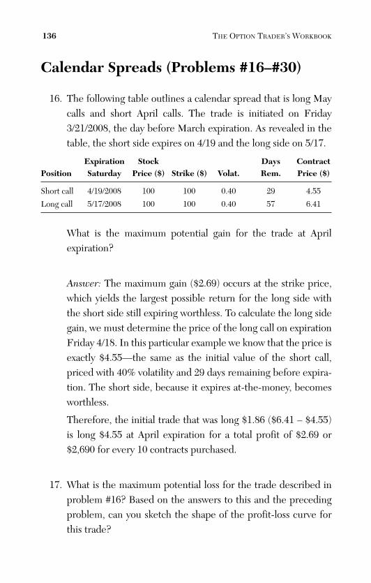
ptg
Calendar Spreads (Problems #16–#30)
16. The following table outlines a calendar spread that is long Maycalls and short April calls. The trade is initiated on Friday3/21/2008, the day before March expiration. As revealed in thetable, the short side expires on 4/19 and the long side on 5/17.
Expiration Stock Days Contract Position Saturday Price ($) Strike ($) Volat. Rem. Price ($)
Short call 4/19/2008 100 100 0.40 29 4.55
Long call 5/17/2008 100 100 0.40 57 6.41
What is the maximum potential gain for the trade at Aprilexpiration?
Answer: The maximum gain ($2.69) occurs at the strike price,which yields the largest possible return for the long side withthe short side still expiring worthless. To calculate the long sidegain, we must determine the price of the long call on expirationFriday 4/18. In this particular example we know that the price isexactly $4.55—the same as the initial value of the short call,priced with 40% volatility and 29 days remaining before expira-tion. The short side, because it expires at-the-money, becomesworthless.
Therefore, the initial trade that was long $1.86 ($6.41 – $4.55)is long $4.55 at April expiration for a total profit of $2.69 or$2,690 for every 10 contracts purchased.
17. What is the maximum potential loss for the trade described inproblem #16? Based on the answers to this and the precedingproblem, can you sketch the shape of the profit-loss curve forthis trade?
136 THE OPTION TRADER’S WORKBOOK
From the Library of Melissa Wong
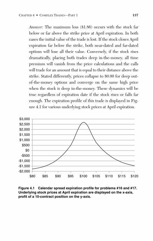
ptg
Answer: The maximum loss ($1.86) occurs with the stock farbelow or far above the strike price at April expiration. In bothcases the initial value of the trade is lost. If the stock closes Aprilexpiration far below the strike, both near-dated and far-datedoptions will lose all their value. Conversely, if the stock risesdramatically, placing both trades deep in-the-money, all timepremium will vanish from the price calculations and the callswill trade for an amount that is equal to their distance above thestrike. Stated differently, prices collapse to $0.00 for deep out-of-the-money options and converge on the same high pricewhen the stock is deep in-the-money. These dynamics will betrue regardless of expiration date if the stock rises or falls farenough. The expiration profile of this trade is displayed in Fig-ure 4.1 for various underlying stock prices at April expiration.
CHAPTER 4 • COMPLEX TRADES—PART 1 137
-$2,000
-$1,500
-$1,000
-$500
$0
$500
$1,000
$1,500
$2,000
$2,500
$3,000
$80 $85 $90 $95 $100 $105 $110 $115 $120
Figure 4.1 Calendar spread expiration profile for problems #16 and #17.Underlying stock prices at April expiration are displayed on the x-axis,profit of a 10-contract position on the y-axis.
From the Library of Melissa Wong
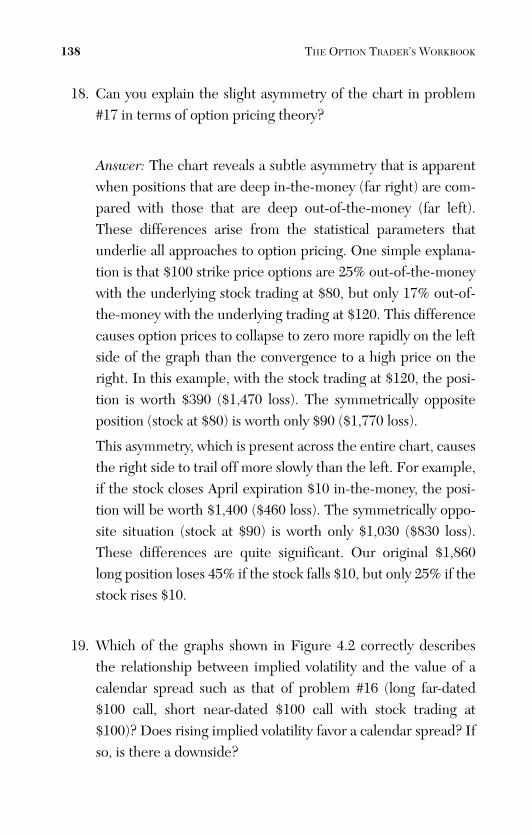
ptg
18. Can you explain the slight asymmetry of the chart in problem#17 in terms of option pricing theory?
Answer: The chart reveals a subtle asymmetry that is apparentwhen positions that are deep in-the-money (far right) are com-pared with those that are deep out-of-the-money (far left).These differences arise from the statistical parameters thatunderlie all approaches to option pricing. One simple explana-tion is that $100 strike price options are 25% out-of-the-moneywith the underlying stock trading at $80, but only 17% out-of-the-money with the underlying trading at $120. This differencecauses option prices to collapse to zero more rapidly on the leftside of the graph than the convergence to a high price on theright. In this example, with the stock trading at $120, the posi-tion is worth $390 ($1,470 loss). The symmetrically oppositeposition (stock at $80) is worth only $90 ($1,770 loss).
This asymmetry, which is present across the entire chart, causesthe right side to trail off more slowly than the left. For example,if the stock closes April expiration $10 in-the-money, the posi-tion will be worth $1,400 ($460 loss). The symmetrically oppo-site situation (stock at $90) is worth only $1,030 ($830 loss).These differences are quite significant. Our original $1,860long position loses 45% if the stock falls $10, but only 25% if thestock rises $10.
19. Which of the graphs shown in Figure 4.2 correctly describesthe relationship between implied volatility and the value of acalendar spread such as that of problem #16 (long far-dated$100 call, short near-dated $100 call with stock trading at$100)? Does rising implied volatility favor a calendar spread? Ifso, is there a downside?
138 THE OPTION TRADER’S WORKBOOK
From the Library of Melissa Wong
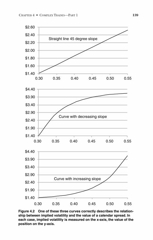
ptg
Figure 4.2 One of these three curves correctly describes the relation-ship between implied volatility and the value of a calendar spread. Ineach case, implied volatility is measured on the x-axis, the value of theposition on the y-axis.
CHAPTER 4 • COMPLEX TRADES—PART 1 139
$1.40
$1.60
$1.80
$2.00
$2.20
$2.40
$2.60
Straight line 45 degree slope
0.30 0.35 0.40 0.45 0.50 0.55
$1.40
$1.90
$2.40
$2.90
$3.40
$3.90
$4.40
0.30 0.35 0.40 0.45 0.50 0.55
Curve with decreasing slope
$1.40
$1.90
$2.40
$2.90
$3.40
$3.90
$4.40
0.30 0.35 0.40 0.45 0.50
Curve with increasing slope
0.55
From the Library of Melissa Wong
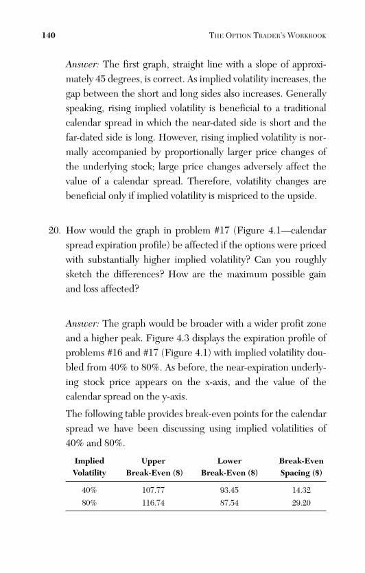
ptg
Answer: The first graph, straight line with a slope of approxi-mately 45 degrees, is correct. As implied volatility increases, thegap between the short and long sides also increases. Generallyspeaking, rising implied volatility is beneficial to a traditionalcalendar spread in which the near-dated side is short and thefar-dated side is long. However, rising implied volatility is nor-mally accompanied by proportionally larger price changes ofthe underlying stock; large price changes adversely affect thevalue of a calendar spread. Therefore, volatility changes arebeneficial only if implied volatility is mispriced to the upside.
20. How would the graph in problem #17 (Figure 4.1—calendarspread expiration profile) be affected if the options were pricedwith substantially higher implied volatility? Can you roughlysketch the differences? How are the maximum possible gainand loss affected?
Answer: The graph would be broader with a wider profit zoneand a higher peak. Figure 4.3 displays the expiration profile ofproblems #16 and #17 (Figure 4.1) with implied volatility dou-bled from 40% to 80%. As before, the near-expiration underly-ing stock price appears on the x-axis, and the value of thecalendar spread on the y-axis.
The following table provides break-even points for the calendarspread we have been discussing using implied volatilities of40% and 80%.
Implied Upper Lower Break-Even Volatility Break-Even ($) Break-Even ($) Spacing ($)
40% 107.77 93.45 14.32
80% 116.74 87.54 29.20
140 THE OPTION TRADER’S WORKBOOK
From the Library of Melissa Wong
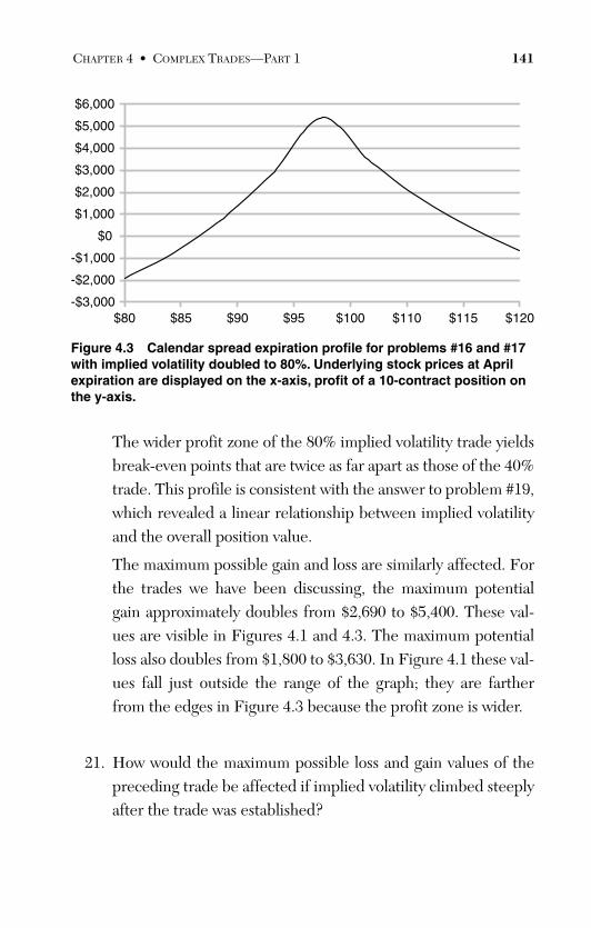
ptg
Figure 4.3 Calendar spread expiration profile for problems #16 and #17with implied volatility doubled to 80%. Underlying stock prices at Aprilexpiration are displayed on the x-axis, profit of a 10-contract position onthe y-axis.
The wider profit zone of the 80% implied volatility trade yieldsbreak-even points that are twice as far apart as those of the 40%trade. This profile is consistent with the answer to problem #19,which revealed a linear relationship between implied volatilityand the overall position value.
The maximum possible gain and loss are similarly affected. Forthe trades we have been discussing, the maximum potentialgain approximately doubles from $2,690 to $5,400. These val-ues are visible in Figures 4.1 and 4.3. The maximum potentialloss also doubles from $1,800 to $3,630. In Figure 4.1 these val-ues fall just outside the range of the graph; they are fartherfrom the edges in Figure 4.3 because the profit zone is wider.
21. How would the maximum possible loss and gain values of thepreceding trade be affected if implied volatility climbed steeplyafter the trade was established?
CHAPTER 4 • COMPLEX TRADES—PART 1 141
-$3,000
-$2,000
-$1,000
$0
$1,000
$2,000
$3,000
$4,000
$5,000
$6,000
$80 $85 $90 $95 $100 $110 $115 $120
From the Library of Melissa Wong
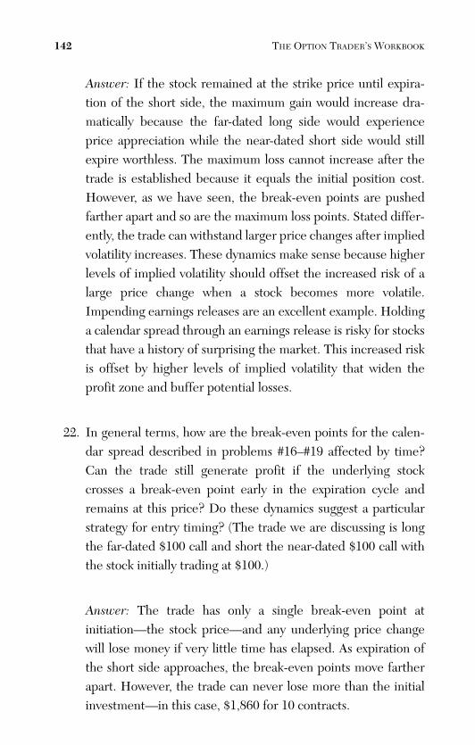
ptg
Answer: If the stock remained at the strike price until expira-tion of the short side, the maximum gain would increase dra-matically because the far-dated long side would experienceprice appreciation while the near-dated short side would stillexpire worthless. The maximum loss cannot increase after thetrade is established because it equals the initial position cost.However, as we have seen, the break-even points are pushedfarther apart and so are the maximum loss points. Stated differ-ently, the trade can withstand larger price changes after impliedvolatility increases. These dynamics make sense because higherlevels of implied volatility should offset the increased risk of alarge price change when a stock becomes more volatile.Impending earnings releases are an excellent example. Holdinga calendar spread through an earnings release is risky for stocksthat have a history of surprising the market. This increased riskis offset by higher levels of implied volatility that widen theprofit zone and buffer potential losses.
22. In general terms, how are the break-even points for the calen-dar spread described in problems #16–#19 affected by time?Can the trade still generate profit if the underlying stockcrosses a break-even point early in the expiration cycle andremains at this price? Do these dynamics suggest a particularstrategy for entry timing? (The trade we are discussing is longthe far-dated $100 call and short the near-dated $100 call withthe stock initially trading at $100.)
Answer: The trade has only a single break-even point atinitiation—the stock price—and any underlying price changewill lose money if very little time has elapsed. As expiration ofthe short side approaches, the break-even points move fartherapart. However, the trade can never lose more than the initialinvestment—in this case, $1,860 for 10 contracts.
142 THE OPTION TRADER’S WORKBOOK
From the Library of Melissa Wong
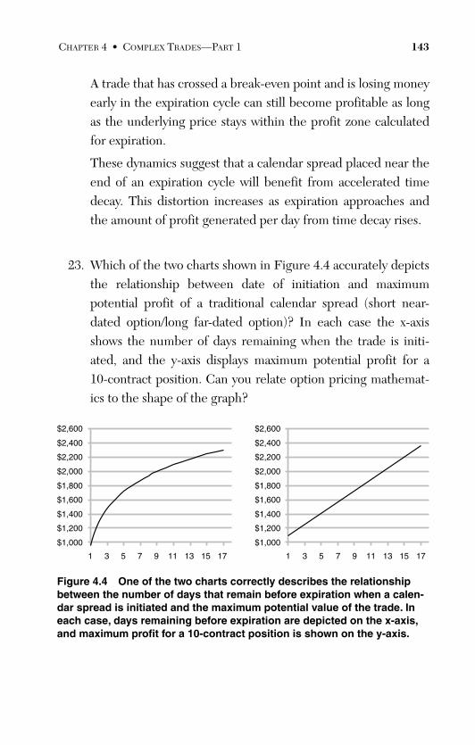
ptg
A trade that has crossed a break-even point and is losing moneyearly in the expiration cycle can still become profitable as longas the underlying price stays within the profit zone calculatedfor expiration.
These dynamics suggest that a calendar spread placed near theend of an expiration cycle will benefit from accelerated timedecay. This distortion increases as expiration approaches andthe amount of profit generated per day from time decay rises.
23. Which of the two charts shown in Figure 4.4 accurately depictsthe relationship between date of initiation and maximumpotential profit of a traditional calendar spread (short near-dated option/long far-dated option)? In each case the x-axisshows the number of days remaining when the trade is initi-ated, and the y-axis displays maximum potential profit for a10-contract position. Can you relate option pricing mathemat-ics to the shape of the graph?
CHAPTER 4 • COMPLEX TRADES—PART 1 143
$1,000
$1,200
$1,400
$1,600
$1,800
$2,000
$2,200
$2,400
$2,600
1 3 5 7 9 11 13 15 17
$1,000
$1,200
$1,400
$1,600
$1,800
$2,000
$2,200
$2,400
$2,600
1 3 5 7 9 11 13 15 17
Figure 4.4 One of the two charts correctly describes the relationshipbetween the number of days that remain before expiration when a calen-dar spread is initiated and the maximum potential value of the trade. Ineach case, days remaining before expiration are depicted on the x-axis,and maximum profit for a 10-contract position is shown on the y-axis.
From the Library of Melissa Wong
ptg
Answer: The first graph (curve with decreasing slope) depictsthe relationship between date of initiation and maximumpotential profit of a calendar spread that is short a near-datedoption and long a far-dated option. Time decay tends to acceler-ate as expiration approaches near the left side of the chart. Theeffect becomes very pronounced when fewer than 2 weeksremain before expiration. The second chart could be correctonly if time decay were a constant process that did not acceler-ate. In this model, an at-the-money option with 30 days remain-ing would be worth precisely 10 times as much as the sameoption with 3 days; sellers of short-term options would beoverly compensated for risk.
24. Without knowing the exact option prices, can you predict whichof the two trades shown in the following table would generatethe largest profit if the stock remains at the strike price untilApril expiration? Which delivers the most profit per day?
Stock Days Position Price ($) Strike ($) Volatility Remaining
Short call 100 100 0.40 30
Long call 100 100 0.40 58
Short call 100 100 0.40 4
Long call 100 100 0.40 32
Answer: Based on the previous discussion, we can predict thatthe maximum profit is larger for the longer-dated trade (firstpair in the table). However, despite the brief timeframe, thesecond trade delivers much more profit per day because ofaccelerated time decay near the end of the expiration cycle.
The next problem will explore risk-based calculations that willfurther test these assumptions.
144 THE OPTION TRADER’S WORKBOOK
From the Library of Melissa Wong
ptg
25. The following table extends the preceding problem with optionprices, break-even points, and maximum potential profit foreach position. Pricing data at April expiration with the stocktrading at $100 is included for reference (pair of entries belowthe gray line). Note that 1 day remains in the contracts becausethey are priced at the close on expiration Friday. As before,both positions are $100 calendar spreads, the stock is trading at$100 when each position is initiated, and implied volatility is40%. Using this data, can you compare the risk-adjustedreturns for the two trades?
Low HighDays Contr. Position Max Break- Break-
Position Rem. Price ($) Contr. Total ($) Profit ($) Even Even
Short call 30 4.63 10
Long call 58 6.47 10 1840 2690 93.38 107.85
Short call 4 1.68 10
Long call 32 4.79 10 3110 1420 96.94 103.48
Short call 1 0.02 10
Long call 29 4.55 10 4530
Answer: Because the timeframes differ, we need to transformthe distance from $100 to each break-even point into standarddeviations before comparing the trades. Following are the cal-culations for both high and low break-evens.
30 Days Remaining
Timeframes in 1 year 365 / 30 = 12.17Annualization factor Sqrt (12.17) = 3.49Volatility for 1 month 0.4 / 3.49 = 0.1151 StdDev change 0.115 × $100 = $11.50
Distance to high break-even $107.85 – $100 = $7.85High break-even StdDev $7.85 / $11.50 = 0.68 StdDev
CHAPTER 4 • COMPLEX TRADES—PART 1 145
From the Library of Melissa Wong
ptg
Distance to low break-even $100 – $93.38 = $6.62Low break-even StdDev $6.62 / $11.50 = 0.58 StdDev
4 Days Remaining
Timeframes in 1 year 365 / 4 = 91.25Annualization factor Sqrt (91.25) = 9.55Volatility for 4 days 0.4 / 9.55 = 0.0421 StdDev change 0.042 × $100 = $4.20
Distance to high break-even $103.48 – $100 = $3.48High break-even StdDev $3.48 / $4.20 = 0.83 StdDev
Distance to low break-even $100 – $96.94 = $3.06Low break-even StdDev $3.06 / $4.20 = 0.73 StdDev
These calculations reveal that the distance to each high or lowbreak-even point is relatively small—less than 1 StdDev. The30-day trade averages 0.63 StdDev and the 4-day trade aver-ages 0.78 StdDev. The differences are minor. In the 4-day caseapproximately 42% of all price changes can be expected to falloutside the break-even point; the figure rises to 52% for the30-day case. We will explore the use of the cumulative normaldistribution function to calculate the percent chance of a pricechange falling within the profit zone in problem #28.
On a risk-adjusted basis, therefore, the return is much smallerfor the 4-day trade because the maximum potential gain isroughly half ($1,440 versus $2,710) and the maximum possibleloss is 69% larger ($3,110 versus $1,840). These dynamics makesense because the timeframe is much shorter and it should notbe possible to consistently generate the same return in 4 days as
146 THE OPTION TRADER’S WORKBOOK
From the Library of Melissa Wong
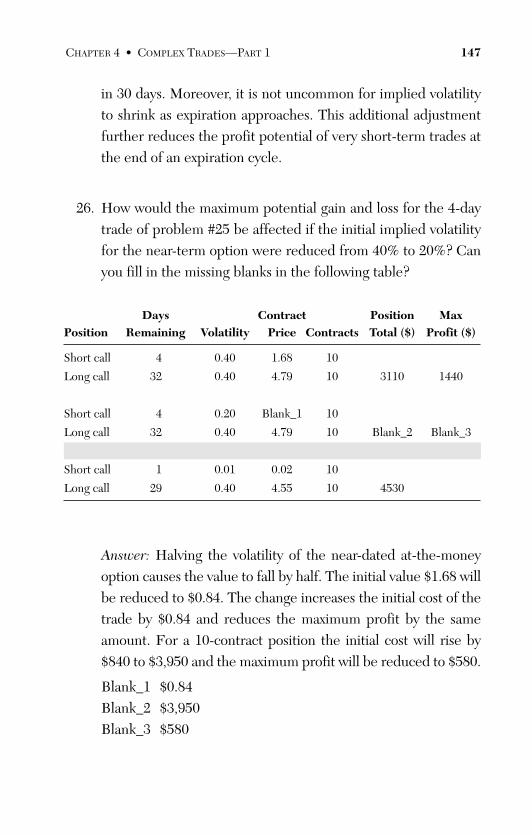
ptg
in 30 days. Moreover, it is not uncommon for implied volatilityto shrink as expiration approaches. This additional adjustmentfurther reduces the profit potential of very short-term trades atthe end of an expiration cycle.
26. How would the maximum potential gain and loss for the 4-daytrade of problem #25 be affected if the initial implied volatilityfor the near-term option were reduced from 40% to 20%? Canyou fill in the missing blanks in the following table?
Days Contract Position MaxPosition Remaining Volatility Price Contracts Total ($) Profit ($)
Short call 4 0.40 1.68 10
Long call 32 0.40 4.79 10 3110 1440
Short call 4 0.20 Blank_1 10
Long call 32 0.40 4.79 10 Blank_2 Blank_3
Short call 1 0.01 0.02 10
Long call 29 0.40 4.55 10 4530
Answer: Halving the volatility of the near-dated at-the-moneyoption causes the value to fall by half. The initial value $1.68 willbe reduced to $0.84. The change increases the initial cost of thetrade by $0.84 and reduces the maximum profit by the sameamount. For a 10-contract position the initial cost will rise by$840 to $3,950 and the maximum profit will be reduced to $580.
Blank_1 $0.84Blank_2 $3,950Blank_3 $580
CHAPTER 4 • COMPLEX TRADES—PART 1 147
From the Library of Melissa Wong
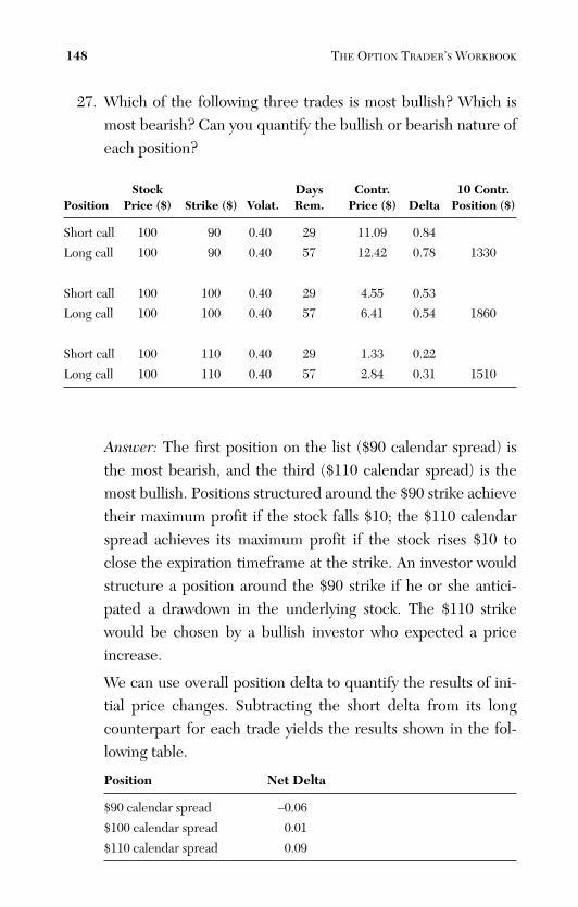
ptg
27. Which of the following three trades is most bullish? Which ismost bearish? Can you quantify the bullish or bearish nature ofeach position?
Stock Days Contr. 10 Contr.Position Price ($) Strike ($) Volat. Rem. Price ($) Delta Position ($)
Short call 100 90 0.40 29 11.09 0.84
Long call 100 90 0.40 57 12.42 0.78 1330
Short call 100 100 0.40 29 4.55 0.53
Long call 100 100 0.40 57 6.41 0.54 1860
Short call 100 110 0.40 29 1.33 0.22
Long call 100 110 0.40 57 2.84 0.31 1510
Answer: The first position on the list ($90 calendar spread) isthe most bearish, and the third ($110 calendar spread) is themost bullish. Positions structured around the $90 strike achievetheir maximum profit if the stock falls $10; the $110 calendarspread achieves its maximum profit if the stock rises $10 toclose the expiration timeframe at the strike. An investor wouldstructure a position around the $90 strike if he or she antici-pated a drawdown in the underlying stock. The $110 strikewould be chosen by a bullish investor who expected a priceincrease.
We can use overall position delta to quantify the results of ini-tial price changes. Subtracting the short delta from its longcounterpart for each trade yields the results shown in the fol-lowing table.
Position Net Delta
$90 calendar spread –0.06
$100 calendar spread 0.01
$110 calendar spread 0.09
148 THE OPTION TRADER’S WORKBOOK
From the Library of Melissa Wong
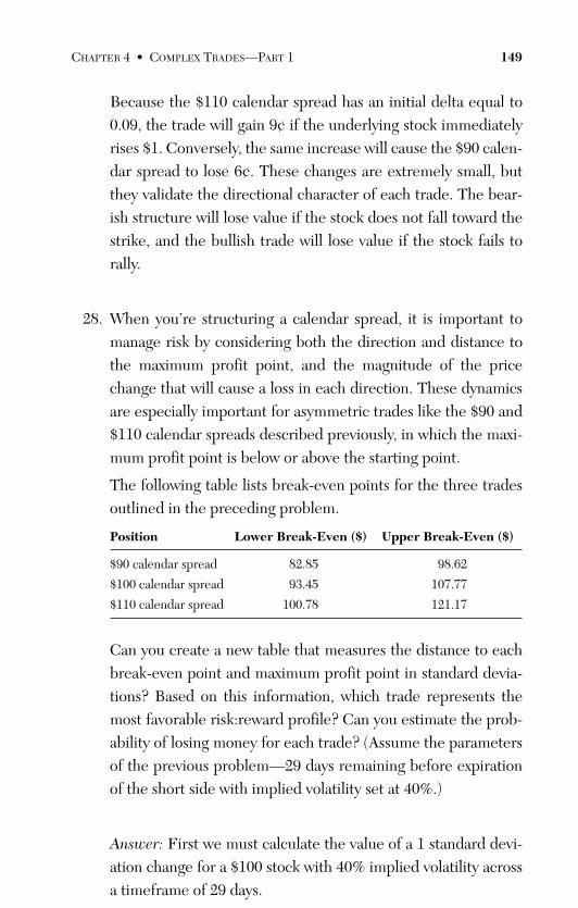
ptg
Because the $110 calendar spread has an initial delta equal to0.09, the trade will gain 9¢ if the underlying stock immediatelyrises $1. Conversely, the same increase will cause the $90 calen-dar spread to lose 6¢. These changes are extremely small, butthey validate the directional character of each trade. The bear-ish structure will lose value if the stock does not fall toward thestrike, and the bullish trade will lose value if the stock fails torally.
28. When you’re structuring a calendar spread, it is important tomanage risk by considering both the direction and distance tothe maximum profit point, and the magnitude of the pricechange that will cause a loss in each direction. These dynamicsare especially important for asymmetric trades like the $90 and$110 calendar spreads described previously, in which the maxi-mum profit point is below or above the starting point.
The following table lists break-even points for the three tradesoutlined in the preceding problem.
Position Lower Break-Even ($) Upper Break-Even ($)
$90 calendar spread 82.85 98.62
$100 calendar spread 93.45 107.77
$110 calendar spread 100.78 121.17
Can you create a new table that measures the distance to eachbreak-even point and maximum profit point in standard devia-tions? Based on this information, which trade represents themost favorable risk:reward profile? Can you estimate the prob-ability of losing money for each trade? (Assume the parametersof the previous problem—29 days remaining before expirationof the short side with implied volatility set at 40%.)
Answer: First we must calculate the value of a 1 standard devi-ation change for a $100 stock with 40% implied volatility acrossa timeframe of 29 days.
CHAPTER 4 • COMPLEX TRADES—PART 1 149
From the Library of Melissa Wong
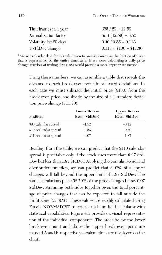
ptg
Timeframes in 1 year1 365 / 29 = 12.59Annualization factor Sqrt (12.59) = 3.55Volatility for 29 days 0.40 / 3.55 = 0.1131 StdDev change 0.113 × $100 = $11.30
1 We use calendar days for this calculation to precisely measure the fraction of a yearthat is represented by the entire timeframe. If we were calculating a daily pricechange, number of trading days (252) would provide a more appropriate metric.
Using these numbers, we can assemble a table that reveals thedistance to each break-even point in standard deviations. Ineach case we must subtract the initial price ($100) from thebreak-even price, and divide by the size of a 1 standard devia-tion price change ($11.30).
Lower Break- Upper Break-Position Even (StdDev) Even (StdDev)
$90 calendar spread –1.52 –0.12
$100 calendar spread –0.58 0.69
$110 calendar spread 0.07 1.87
Reading from the table, we can predict that the $110 calendarspread is profitable only if the stock rises more than 0.07 Std-Dev but less than 1.87 StdDev. Applying the cumulative normaldistribution function, we can predict that 3.07% of all pricechanges will fall beyond the upper limit of 1.87 StdDev. Thesame calculations place 52.79% of the price changes below 0.07StdDev. Summing both sides together gives the total percent-age of price changes that can be expected to fall outside theprofit zone (55.86%). These values are readily calculated usingExcel’s NORMSDIST function or a hand-held calculator withstatistical capabilities. Figure 4.5 provides a visual representa-tion of the individual components. The areas below the lowerbreak-even point and above the upper break-even point aremarked A and B respectively—calculations are displayed on thechart.
150 THE OPTION TRADER’S WORKBOOK
From the Library of Melissa Wong
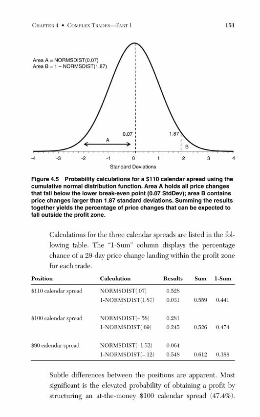
ptg
Figure 4.5 Probability calculations for a $110 calendar spread using thecumulative normal distribution function. Area A holds all price changesthat fall below the lower break-even point (0.07 StdDev); area B containsprice changes larger than 1.87 standard deviations. Summing the resultstogether yields the percentage of price changes that can be expected tofall outside the profit zone.
Calculations for the three calendar spreads are listed in the fol-lowing table. The “1-Sum” column displays the percentagechance of a 29-day price change landing within the profit zonefor each trade.
Position Calculation Results Sum 1-Sum
$110 calendar spread NORMSDIST(.07) 0.528
1-NORMSDIST(1.87) 0.031 0.559 0.441
$100 calendar spread NORMSDIST(–.58) 0.281
1-NORMSDIST(.69) 0.245 0.526 0.474
$90 calendar spread NORMSDIST(–1.52) 0.064
1-NORMSDIST(–.12) 0.548 0.612 0.388
Subtle differences between the positions are apparent. Mostsignificant is the elevated probability of obtaining a profit bystructuring an at-the-money $100 calendar spread (47.4%).
CHAPTER 4 • COMPLEX TRADES—PART 1 151
Standard Deviations
Area A = NORMSDIST(0.07)Area B = 1 – NORMSDIST(1.87)
0.07A
-4 -3 -2 -1 0 1 2 43
B
1.87
From the Library of Melissa Wong
ptg
Overall, however, the differences are relatively small, and aninvestor considering one of these trades would likely choose astrike price based on a bearish or bullish view of the underlyingstock.
29. The following table contains two calendar spreads spanning dif-ferent timeframes. In both cases the near-dated short sideexpires in 29 days. The long side of the first trade expires in 57days; the long side of the second trade has a longer time-frame—183 days. Can you fill in the blanks and determine themaximum profit for the second trade? How would you rational-ize these results with regard to time decay?
Stock Days Contr. Pos. MaxPosition Price ($) Strike ($) Rem. Price ($) Total ($) Theta Profit ($)
Short call 100 100 29 4.55 –0.079
Long call 100 100 57 6.41 1.86 –0.057 2.67
Short call 100 100 1 0.02 –0.020
Long call 100 100 29 4.55 4.53 –0.079
Short call 100 100 29 4.55 –0.079
Long call 100 100 183 11.60 7.05 –0.032 Blank_3
Short call 100 100 1 0.02 –0.020
Long call 100 100 155 Blank_1 Blank_2 –0.035
Answer: Far-dated at-the-money options exhibit relatively flattime decay. This effect is visible in the table because theta forthe second trade barely increases from –0.032 to –0.035 duringthe first month. Multiplying the average value (–0.0335) by thenumber of days that elapse (28) provides an exact value for theamount of time premium lost in the long side of the trade(–0.0335 × 28 = $0.94). Subtracting 94¢ from the original value($11.60) yields a new value for the long $100 call with 155 days
152 THE OPTION TRADER’S WORKBOOK
From the Library of Melissa Wong
ptg
remaining ($10.66). Subtracting the tiny amount of premium(2¢) left in the short side gives a position total of $10.64. Finally,we can determine the maximum profit by subtracting the origi-nal position cost ($10.64 – $7.05 = $3.59). The answers aresummarized here.
Blank_1 $10.66Blank_2 $10.64Blank_3 $3.59
30. The results of problem #29 seem to suggest that the profit of acalendar spread increases with the time gap between the twosides. Is there a downside to this trade structure? Would takingthe other side of the trade—short the far-dated option/long thenear-dated option—be a better choice from a risk:rewardperspective?
Answer: Unfortunately, the profit of the second trade is muchsmaller than that of the first when measured as a percentage ofthe original investment. The first trade (28-day spacing) has amaximum profit potential of $2.67 or 144% of the original pur-chase price; the second trade (154-day spacing) generates moreabsolute profit ($3.59), but on a much larger initial investment($7.05). In percentage terms, the second trade has a maximumpotential return of only 51%.
Statistically speaking, it would make more sense to structurethe second trade as a reverse calendar spread—short the far-dated side and long the near-dated side. Reversing our previouscalculations yields a maximum potential gain of $7.05 against a$3.59 downside risk.
CHAPTER 4 • COMPLEX TRADES—PART 1 153
From the Library of Melissa Wong
ptg
Diagonal Calendar Spreads SpanningMultiple Expirations and Strike Prices(Problems #31–#34)
31. The following table contains relevant pricing information forthree different trades. Each is represented by a pair of entriescomposed of a short side and a long side. The trades are eachinitiated on Friday 3/21/2008, the day before March expiration.All three short sides expire on Saturday 4/19, the long sidesexpire on Saturday 5/17. Which of the three is most bullish andwhich is most bearish? How do the three trades compare withthe stock trading at $105 at April expiration? Do the positiondeltas provide useful evidence?
Stock Implied Days Exp. Contr.Position Price ($) Strike($) Volat. Delta Theta Rem. Sat. Price ($)
Short call 100 105 0.40 0.36 –0.07 29 4/19 2.57
Long call 100 110 0.40 0.31 –0.05 57 5/17 2.84
Short call 100 105 0.40 0.36 –0.07 29 4/19 2.57
Long call 100 100 0.40 0.54 –0.06 57 5/17 6.41
Short call 100 110 0.40 0.22 –0.06 29 4/19 1.33
Long call 100 105 0.40 0.41 –0.06 57 5/17 4.35
Answer: The first trade (short $105/long $110) is the most bear-ish and the third (short $110/long $105) is the most bullish.
Trade #1
The first trade is initially long just 27¢. Maximum profit is real-ized at near-term expiration with the stock trading at $105. Inthis situation $2.57 of profit is realized from the short sale, andthe long side will be worth approximately the same as its initialcost. We can estimate this value from the short side, which isinitially $5.00 out-of-the-money with 29 days remaining. When
154 THE OPTION TRADER’S WORKBOOK
From the Library of Melissa Wong
ptg
the short side closes on 4/18, the long side will also have 29 daysremaining. We can add a small premium (20¢) to account forthe $5.00 increase in the underlying stock price. Using thesedynamics, we can predict that the trade will yield a maximumprofit of around $2.50.
If the stock rises sharply, the short side will be worth $5.00more than the long side—that is, the position will transitionfrom long $0.27 to short approximately $5.00 ($5.27 loss). Con-versely, the maximum loss that can be realized in a price declineis the initial 27¢ paid for the trade.
Trade #2
The second trade achieves its largest gain if the stock closes at$105 on Friday 4/18 and the cost of the short side is realized as$2.57 of profit. To estimate the value of the long side, which isnow $5.00 in-the-money, we must add a factor to account for theremaining 29 days of time decay. Early in the expiration cyclewith 57 days remaining, theta was equal to 6¢ per day. It is rea-sonable to add 50% to this number to account for acceleratedtime decay that will occur as the end of the expiration cycleapproaches. We can, therefore, estimate that time decay will add$2.61 to the option price ($0.09 × 29 days). Adding this value tothe amount that the options are in-the-money ($5.00) yields avalue of $7.61—a $1.20 profit for the long side. This value canbe confirmed with a Black-Scholes calculator. Surprisingly, theestimate is exactly correct. By combining the profits of bothsides, we can accurately estimate that the trade returns $3.77($2.57 from the short side and $1.20 from the long side).
If the stock rises sharply, placing both sides of the trade far in-the-money, the value will be equal to the difference betweenthe strikes ($5.00). Subtracting the cost of the initial trade($3.84) yields a total profit of $1.16. Conversely, the maximumloss that can be realized if the price declines sharply is equal tothe initial purchase price ($3.84).
CHAPTER 4 • COMPLEX TRADES—PART 1 155
From the Library of Melissa Wong
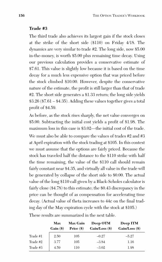
ptg
Trade #3
The third trade also achieves its largest gain if the stock closesat the strike of the short side ($110) on Friday 4/18. Thedynamics are very similar to trade #2. The long side, now $5.00in-the-money, is worth $5.00 plus remaining time decay. Usingour previous calculation provides a conservative estimate of$7.61. This value is slightly low because it is based on the timedecay for a much less expensive option that was priced beforethe stock climbed $10.00. However, despite the conservativenature of the estimate, the profit is still larger than that of trade#2. The short side generates a $1.33 return; the long side yields$3.26 ($7.61 – $4.35). Adding these values together gives a totalprofit of $4.59.
As before, as the stock rises sharply, the net value converges on$5.00. Subtracting the initial cost yields a profit of $1.98. Themaximum loss in this case is $3.02—the initial cost of the trade.
We must also be able to compare the values of trades #2 and #3at April expiration with the stock trading at $105. In this contextwe must assume that the options are fairly priced. Because thestock has traveled half the distance to the $110 strike with halfthe time remaining, the value of the $110 call should remainfairly constant near $4.35, and virtually all value in the trade willbe generated by collapse of the short side to $0.00. The actualvalue of the long $110 call given by a Black-Scholes calculator isfairly close ($4.78) to this estimate; the $0.43 discrepancy in theprice can be thought of as compensation for accelerating timedecay. (Actual value of theta increases to 44¢ on the final trad-ing day of the May expiration cycle with the stock at $105.)
These results are summarized in the next table.
Max Max Gain Deep OTM Deep ITMGain ($) Price ($) Gain/Loss ($) Gain/Loss ($)
Trade #1 2.50 105 –0.27 –5.27
Trade #2 3.77 105 –3.84 1.16
Trade #3 4.59 110 –3.02 1.98
156 THE OPTION TRADER’S WORKBOOK
From the Library of Melissa Wong
ptg
The bearish nature of the first trade is evident in the substantial($5.27) loss that occurs when the underlying stock price risessharply. The trade is also hedged against very large pricedeclines because the prices and deltas of both sides are nearlyequal. While clearly the most bearish of the group, it is notdesigned to profit from a large price decline.
Both trade #2 and trade #3 are bullish because they aredesigned to profit from large price increases. Trade #3 is morebullish because it anticipates a larger price increase. Its maxi-mum gain is 22% larger, occurs $5.00 farther in-the-money, andis capped at a higher price ($1.98 versus $1.16). Furthermore,the trade will generate a substantially smaller gain than trade #2if the stock rises only $5.00 by April expiration. As discussedpreviously, the long side just keeps pace with time decay, andvirtually all profit is generated by collapse of the short side from$1.33 to $0.00. In summary, trade #2 generates nearly threetimes as much profit as trade #3 if the stock closes April expira-tion at $105—further evidence that trade #3 is built around amore bullish view.
Differences between long and short deltas are virtually identi-cal for both trades. However, because the deltas are uniformlylower for trade #3, it can be concluded that both sides are far-ther out-of-the-money when the trade is initiated. Increaseddistance to the strikes provides additional verification that thetrade is structured around larger underlying price changes.
32. The three graphs shown in Figure 4.6 are profit profiles for thetrades outlined in problem #31. In each case the stock price atApril expiration is represented on the x-axis, and position valueis measured on the y-axis (unlabeled). Can you match eachtrade to its corresponding profile?
CHAPTER 4 • COMPLEX TRADES—PART 1 157
From the Library of Melissa Wong
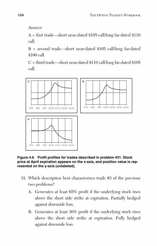
ptg
Figure 4.6 Profit profiles for trades described in problem #31. Stockprice at April expiration appears on the x-axis, and position value is rep-resented on the y-axis (unlabeled).
33. Which description best characterizes trade #3 of the previoustwo problems?
A. Generates at least 65% profit if the underlying stock risesabove the short side strike at expiration. Partially hedgedagainst downside loss.
B. Generates at least 30% profit if the underlying stock risesabove the short side strike at expiration. Fully hedgedagainst downside loss.
158 THE OPTION TRADER’S WORKBOOK
$95 $105 $115 $125 $135$75 $85
$95 $105 $115 $125 $135$75 $85 $95 $105 $115 $125 $135$75 $85
C
A
B
Answer:
A = first trade—short near-dated $105 call/long far-dated $110call.
B = second trade—short near-dated $105 call/long far-dated$100 call.
C = third trade—short near-dated $110 call/long far-dated $105call.
From the Library of Melissa Wong
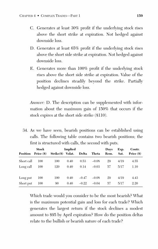
ptg
C. Generates at least 30% profit if the underlying stock risesabove the short strike at expiration. Not hedged againstdownside loss.
D. Generates at least 65% profit if the underlying stock risesabove the short side strike at expiration. Not hedged againstdownside loss.
E. Generates more than 100% profit if the underlying stockrises above the short side strike at expiration. Value of theposition declines steadily beyond the strike. Partiallyhedged against downside loss.
Answer: D. The description can be supplemented with infor-mation about the maximum gain of 150% that occurs if thestock expires at the short side strike ($110).
34. As we have seen, bearish positions can be established usingcalls. The following table contains two bearish positions; thefirst is structured with calls, the second with puts.
Stock Implied Days Exp. Contr.Position Price ($) Strike($) Volat. Delta Theta Rem. Sat. Price ($)
Short call 100 100 0.40 0.53 –0.08 29 4/19 4.55
Long call 100 120 0.40 0.14 –0.03 57 5/17 1.10
Long put 100 100 0.40 –0.47 –0.08 29 4/19 4.43
Short put 100 90 0.40 –0.22 –0.04 57 5/17 2.20
Which trade would you consider to be the most bearish? Whatis the maximum potential gain and loss for each trade? Whichgenerates the largest return if the stock declines a modestamount to $95 by April expiration? How do the position deltasrelate to the bullish or bearish nature of each trade?
CHAPTER 4 • COMPLEX TRADES—PART 1 159
From the Library of Melissa Wong
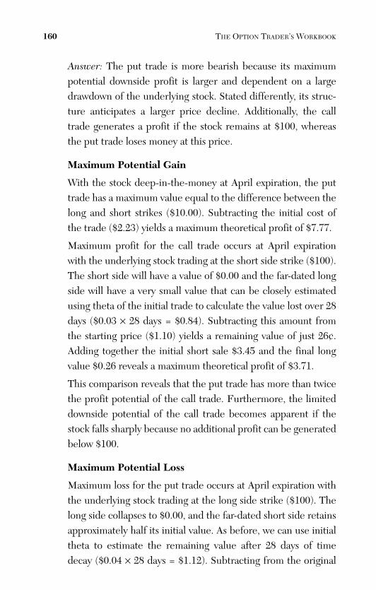
ptg
Answer: The put trade is more bearish because its maximumpotential downside profit is larger and dependent on a largedrawdown of the underlying stock. Stated differently, its struc-ture anticipates a larger price decline. Additionally, the calltrade generates a profit if the stock remains at $100, whereasthe put trade loses money at this price.
Maximum Potential Gain
With the stock deep-in-the-money at April expiration, the puttrade has a maximum value equal to the difference between thelong and short strikes ($10.00). Subtracting the initial cost ofthe trade ($2.23) yields a maximum theoretical profit of $7.77.
Maximum profit for the call trade occurs at April expirationwith the underlying stock trading at the short side strike ($100).The short side will have a value of $0.00 and the far-dated longside will have a very small value that can be closely estimatedusing theta of the initial trade to calculate the value lost over 28days ($0.03 × 28 days = $0.84). Subtracting this amount fromthe starting price ($1.10) yields a remaining value of just 26¢.Adding together the initial short sale $3.45 and the final longvalue $0.26 reveals a maximum theoretical profit of $3.71.
This comparison reveals that the put trade has more than twicethe profit potential of the call trade. Furthermore, the limiteddownside potential of the call trade becomes apparent if thestock falls sharply because no additional profit can be generatedbelow $100.
Maximum Potential Loss
Maximum loss for the put trade occurs at April expiration withthe underlying stock trading at the long side strike ($100). Thelong side collapses to $0.00, and the far-dated short side retainsapproximately half its initial value. As before, we can use initialtheta to estimate the remaining value after 28 days of timedecay ($0.04 × 28 days = $1.12). Subtracting from the original
160 THE OPTION TRADER’S WORKBOOK
From the Library of Melissa Wong
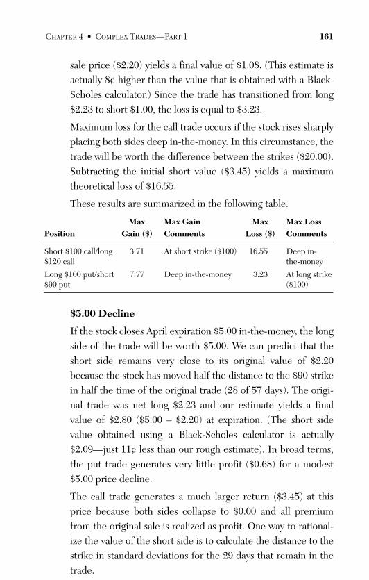
ptg
sale price ($2.20) yields a final value of $1.08. (This estimate isactually 8¢ higher than the value that is obtained with a Black-Scholes calculator.) Since the trade has transitioned from long$2.23 to short $1.00, the loss is equal to $3.23.
Maximum loss for the call trade occurs if the stock rises sharplyplacing both sides deep in-the-money. In this circumstance, thetrade will be worth the difference between the strikes ($20.00).Subtracting the initial short value ($3.45) yields a maximumtheoretical loss of $16.55.
These results are summarized in the following table.
Max Max Gain Max Max LossPosition Gain ($) Comments Loss ($) Comments
Short $100 call/long 3.71 At short strike ($100) 16.55 Deep in-$120 call the-money
Long $100 put/short 7.77 Deep in-the-money 3.23 At long strike $90 put ($100)
$5.00 Decline
If the stock closes April expiration $5.00 in-the-money, the longside of the trade will be worth $5.00. We can predict that theshort side remains very close to its original value of $2.20because the stock has moved half the distance to the $90 strikein half the time of the original trade (28 of 57 days). The origi-nal trade was net long $2.23 and our estimate yields a finalvalue of $2.80 ($5.00 – $2.20) at expiration. (The short sidevalue obtained using a Black-Scholes calculator is actually$2.09—just 11¢ less than our rough estimate). In broad terms,the put trade generates very little profit ($0.68) for a modest$5.00 price decline.
The call trade generates a much larger return ($3.45) at thisprice because both sides collapse to $0.00 and all premiumfrom the original sale is realized as profit. One way to rational-ize the value of the short side is to calculate the distance to thestrike in standard deviations for the 29 days that remain in thetrade.
CHAPTER 4 • COMPLEX TRADES—PART 1 161
From the Library of Melissa Wong
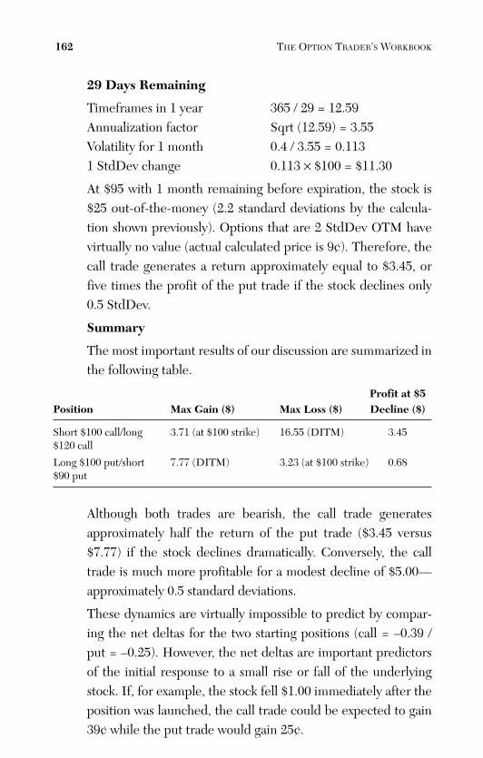
ptg
29 Days Remaining
Timeframes in 1 year 365 / 29 = 12.59Annualization factor Sqrt (12.59) = 3.55Volatility for 1 month 0.4 / 3.55 = 0.1131 StdDev change 0.113 × $100 = $11.30
At $95 with 1 month remaining before expiration, the stock is$25 out-of-the-money (2.2 standard deviations by the calcula-tion shown previously). Options that are 2 StdDev OTM havevirtually no value (actual calculated price is 9¢). Therefore, thecall trade generates a return approximately equal to $3.45, orfive times the profit of the put trade if the stock declines only0.5 StdDev.
Summary
The most important results of our discussion are summarized inthe following table.
Profit at $5Position Max Gain ($) Max Loss ($) Decline ($)
Short $100 call/long 3.71 (at $100 strike) 16.55 (DITM) 3.45$120 call
Long $100 put/short 7.77 (DITM) 3.23 (at $100 strike) 0.68$90 put
Although both trades are bearish, the call trade generatesapproximately half the return of the put trade ($3.45 versus$7.77) if the stock declines dramatically. Conversely, the calltrade is much more profitable for a modest decline of $5.00—approximately 0.5 standard deviations.
These dynamics are virtually impossible to predict by compar-ing the net deltas for the two starting positions (call = –0.39 /put = –0.25). However, the net deltas are important predictorsof the initial response to a small rise or fall of the underlyingstock. If, for example, the stock fell $1.00 immediately after theposition was launched, the call trade could be expected to gain39¢ while the put trade would gain 25¢.
162 THE OPTION TRADER’S WORKBOOK
From the Library of Melissa Wong
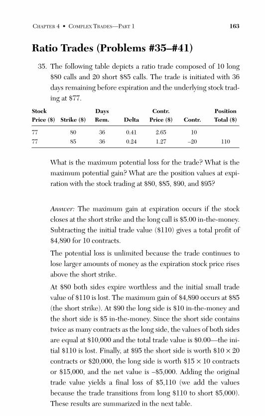
ptg
Ratio Trades (Problems #35–#41)
35. The following table depicts a ratio trade composed of 10 long$80 calls and 20 short $85 calls. The trade is initiated with 36days remaining before expiration and the underlying stock trad-ing at $77.
Stock Days Contr. PositionPrice ($) Strike ($) Rem. Delta Price ($) Contr. Total ($)
77 80 36 0.41 2.65 10
77 85 36 0.24 1.27 –20 110
What is the maximum potential loss for the trade? What is themaximum potential gain? What are the position values at expi-ration with the stock trading at $80, $85, $90, and $95?
Answer: The maximum gain at expiration occurs if the stockcloses at the short strike and the long call is $5.00 in-the-money.Subtracting the initial trade value ($110) gives a total profit of$4,890 for 10 contracts.
The potential loss is unlimited because the trade continues tolose larger amounts of money as the expiration stock price risesabove the short strike.
At $80 both sides expire worthless and the initial small tradevalue of $110 is lost. The maximum gain of $4,890 occurs at $85(the short strike). At $90 the long side is $10 in-the-money andthe short side is $5 in-the-money. Since the short side containstwice as many contracts as the long side, the values of both sidesare equal at $10,000 and the total trade value is $0.00—the ini-tial $110 is lost. Finally, at $95 the short side is worth $10 × 20contracts or $20,000, the long side is worth $15 × 10 contractsor $15,000, and the net value is –$5,000. Adding the originaltrade value yields a final loss of $5,110 (we add the valuesbecause the trade transitions from long $110 to short $5,000).These results are summarized in the next table.
CHAPTER 4 • COMPLEX TRADES—PART 1 163
From the Library of Melissa Wong
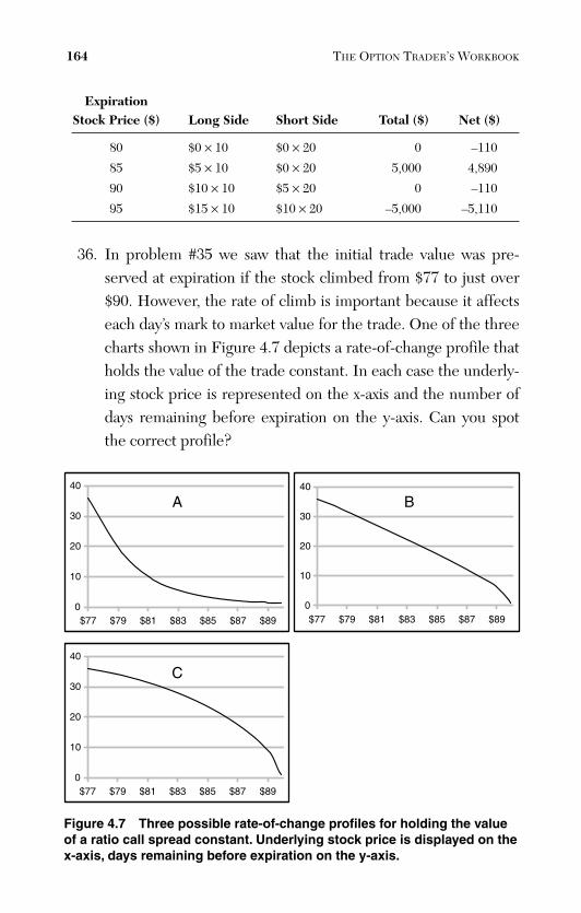
ptg
ExpirationStock Price ($) Long Side Short Side Total ($) Net ($)
80 $0 × 10 $0 × 20 0 –110
85 $5 × 10 $0 × 20 5,000 4,890
90 $10 × 10 $5 × 20 0 –110
95 $15 × 10 $10 × 20 –5,000 –5,110
36. In problem #35 we saw that the initial trade value was pre-served at expiration if the stock climbed from $77 to just over$90. However, the rate of climb is important because it affectseach day’s mark to market value for the trade. One of the threecharts shown in Figure 4.7 depicts a rate-of-change profile thatholds the value of the trade constant. In each case the underly-ing stock price is represented on the x-axis and the number ofdays remaining before expiration on the y-axis. Can you spotthe correct profile?
164 THE OPTION TRADER’S WORKBOOK
0
10
20
30
40
$77 $79 $81 $83 $85 $87 $89 $77 $79 $81 $83 $85 $87 $890
10
20
30
40
$77 $79
A
C
B
$81 $83 $85 $87 $890
10
20
30
40
Figure 4.7 Three possible rate-of-change profiles for holding the valueof a ratio call spread constant. Underlying stock price is displayed on thex-axis, days remaining before expiration on the y-axis.
From the Library of Melissa Wong
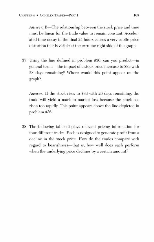
ptg
Answer: B—The relationship between the stock price and timemust be linear for the trade value to remain constant. Acceler-ated time decay in the final 24 hours causes a very subtle pricedistortion that is visible at the extreme right side of the graph.
37. Using the line defined in problem #36, can you predict—ingeneral terms—the impact of a stock price increase to $83 with28 days remaining? Where would this point appear on thegraph?
Answer: If the stock rises to $83 with 26 days remaining, thetrade will yield a mark to market loss because the stock hasrisen too rapidly. This point appears above the line depicted inproblem #36.
38. The following table displays relevant pricing information forfour different trades. Each is designed to generate profit from adecline in the stock price. How do the trades compare withregard to bearishness—that is, how well does each performwhen the underlying price declines by a certain amount?
CHAPTER 4 • COMPLEX TRADES—PART 1 165
From the Library of Melissa Wong
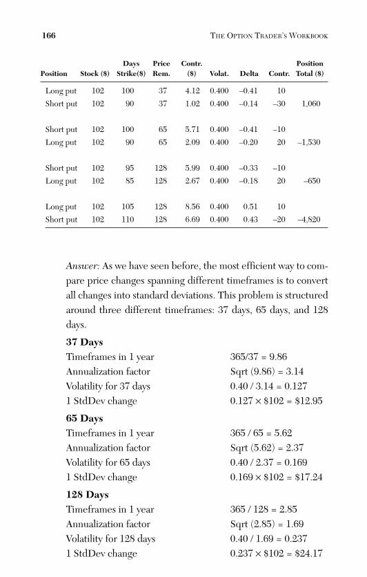
ptg
Days Price Contr. PositionPosition Stock ($) Strike($) Rem. ($) Volat. Delta Contr. Total ($)
Long put 102 100 37 4.12 0.400 –0.41 10
Short put 102 90 37 1.02 0.400 –0.14 –30 1,060
Short put 102 100 65 5.71 0.400 –0.41 –10
Long put 102 90 65 2.09 0.400 –0.20 20 –1,530
Short put 102 95 128 5.99 0.400 –0.33 –10
Long put 102 85 128 2.67 0.400 –0.18 20 –650
Long put 102 105 128 8.56 0.400 0.51 10
Short put 102 110 128 6.69 0.400 0.43 –20 –4,820
Answer: As we have seen before, the most efficient way to com-pare price changes spanning different timeframes is to convertall changes into standard deviations. This problem is structuredaround three different timeframes: 37 days, 65 days, and 128days.
37 DaysTimeframes in 1 year 365/37 = 9.86Annualization factor Sqrt (9.86) = 3.14Volatility for 37 days 0.40 / 3.14 = 0.1271 StdDev change 0.127 × $102 = $12.95
65 DaysTimeframes in 1 year 365 / 65 = 5.62Annualization factor Sqrt (5.62) = 2.37Volatility for 65 days 0.40 / 2.37 = 0.1691 StdDev change 0.169 × $102 = $17.24
128 DaysTimeframes in 1 year 365 / 128 = 2.85Annualization factor Sqrt (2.85) = 1.69Volatility for 128 days 0.40 / 1.69 = 0.2371 StdDev change 0.237 × $102 = $24.17
166 THE OPTION TRADER’S WORKBOOK
From the Library of Melissa Wong
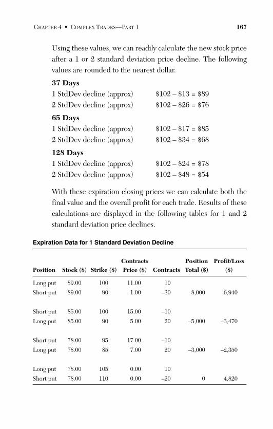
ptg
Using these values, we can readily calculate the new stock priceafter a 1 or 2 standard deviation price decline. The followingvalues are rounded to the nearest dollar.
37 Days1 StdDev decline (approx) $102 – $13 = $892 StdDev decline (approx) $102 – $26 = $76
65 Days1 StdDev decline (approx) $102 – $17 = $852 StdDev decline (approx) $102 – $34 = $68
128 Days1 StdDev decline (approx) $102 – $24 = $782 StdDev decline (approx) $102 – $48 = $54
With these expiration closing prices we can calculate both thefinal value and the overall profit for each trade. Results of thesecalculations are displayed in the following tables for 1 and 2standard deviation price declines.
Expiration Data for 1 Standard Deviation Decline
Contracts Position Profit/LossPosition Stock ($) Strike ($) Price ($) Contracts Total ($) ($)
Long put 89.00 100 11.00 10
Short put 89.00 90 1.00 –30 8,000 6,940
Short put 85.00 100 15.00 –10
Long put 85.00 90 5.00 20 –5,000 –3,470
Short put 78.00 95 17.00 –10
Long put 78.00 85 7.00 20 –3,000 –2,350
Long put 78.00 105 0.00 10
Short put 78.00 110 0.00 –20 0 4,820
CHAPTER 4 • COMPLEX TRADES—PART 1 167
From the Library of Melissa Wong
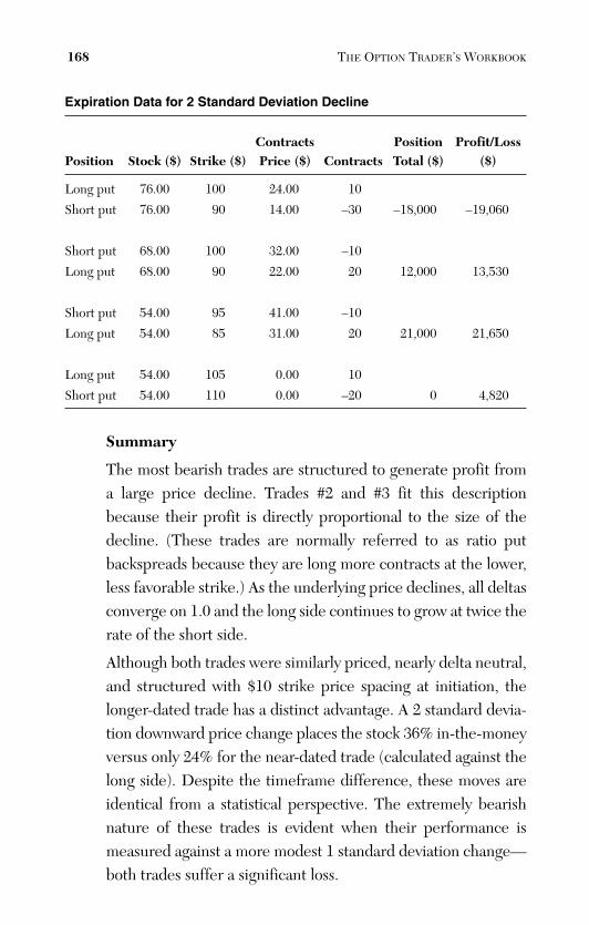
ptg
Expiration Data for 2 Standard Deviation Decline
Contracts Position Profit/LossPosition Stock ($) Strike ($) Price ($) Contracts Total ($) ($)
Long put 76.00 100 24.00 10
Short put 76.00 90 14.00 –30 –18,000 –19,060
Short put 68.00 100 32.00 –10
Long put 68.00 90 22.00 20 12,000 13,530
Short put 54.00 95 41.00 –10
Long put 54.00 85 31.00 20 21,000 21,650
Long put 54.00 105 0.00 10
Short put 54.00 110 0.00 –20 0 4,820
Summary
The most bearish trades are structured to generate profit froma large price decline. Trades #2 and #3 fit this descriptionbecause their profit is directly proportional to the size of thedecline. (These trades are normally referred to as ratio putbackspreads because they are long more contracts at the lower,less favorable strike.) As the underlying price declines, all deltasconverge on 1.0 and the long side continues to grow at twice therate of the short side.
Although both trades were similarly priced, nearly delta neutral,and structured with $10 strike price spacing at initiation, thelonger-dated trade has a distinct advantage. A 2 standard devia-tion downward price change places the stock 36% in-the-moneyversus only 24% for the near-dated trade (calculated against thelong side). Despite the timeframe difference, these moves areidentical from a statistical perspective. The extremely bearishnature of these trades is evident when their performance ismeasured against a more modest 1 standard deviation change—both trades suffer a significant loss.
168 THE OPTION TRADER’S WORKBOOK
From the Library of Melissa Wong
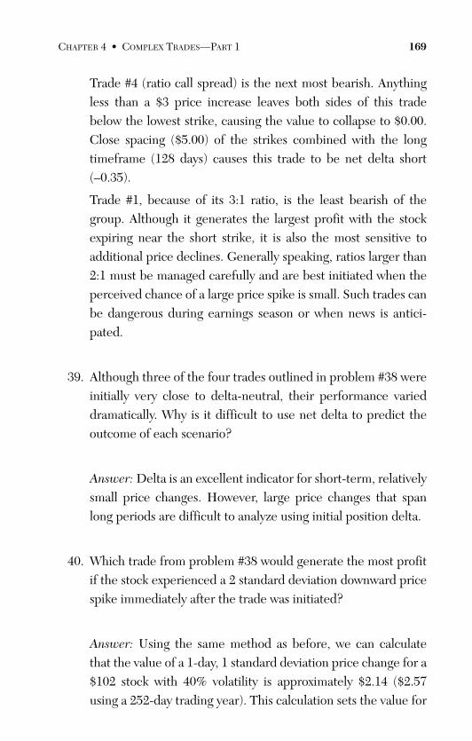
ptg
Trade #4 (ratio call spread) is the next most bearish. Anythingless than a $3 price increase leaves both sides of this tradebelow the lowest strike, causing the value to collapse to $0.00.Close spacing ($5.00) of the strikes combined with the longtimeframe (128 days) causes this trade to be net delta short(–0.35).
Trade #1, because of its 3:1 ratio, is the least bearish of thegroup. Although it generates the largest profit with the stockexpiring near the short strike, it is also the most sensitive toadditional price declines. Generally speaking, ratios larger than2:1 must be managed carefully and are best initiated when theperceived chance of a large price spike is small. Such trades canbe dangerous during earnings season or when news is antici-pated.
39. Although three of the four trades outlined in problem #38 wereinitially very close to delta-neutral, their performance varieddramatically. Why is it difficult to use net delta to predict theoutcome of each scenario?
Answer: Delta is an excellent indicator for short-term, relativelysmall price changes. However, large price changes that spanlong periods are difficult to analyze using initial position delta.
40. Which trade from problem #38 would generate the most profitif the stock experienced a 2 standard deviation downward pricespike immediately after the trade was initiated?
Answer: Using the same method as before, we can calculatethat the value of a 1-day, 1 standard deviation price change for a$102 stock with 40% volatility is approximately $2.14 ($2.57using a 252-day trading year). This calculation sets the value for
CHAPTER 4 • COMPLEX TRADES—PART 1 169
From the Library of Melissa Wong
ptg
a 2 StdDev decline at $97 ($5.00). Such a decline early in theexpiration cycle will have the largest effect on the trade with thelargest delta imbalance—trade #4. The first trade, owing to its3:1 ratio, will also be sensitive to a move of this magnitude,especially since the long side moves from out-of-the-money toin-the-money. As a result, its delta begins to rise significantlymore slowly than the short side. This effect is exaggerated bythe 3:1 ratio.
Although it is not necessary to have a Black-Scholes calculatorto make this prediction, the actual results are interesting; trade#4 (call ratio) generates a $1,590 profit and trade #1 (3:1 putratio) yields a $490 loss. The two put backspreads remain rela-tively unchanged because they are low ratios (2:1), are delta-neutral, and have significant time remaining before expiration.
41. Can you calculate the exact break-even price at expiration forthe trade shown in the following table? What would the generalformula be for calculating the break-even point for any ratiotrade?
Days Contr. Position
Position Stock ($) Strike ($) Rem. Price ($) Contr. Total ($) Net
Long call 128 130 33 6.85 15 10,275
Short call 128 145 33 2.37 –50 –11,850 –1,575
Answer: The expiration value of the short side is given by5,000 × (exp – $145)
where exp is the stock price. Similarly, the value of the longside is given by1,500 × (exp – $130)
170 THE OPTION TRADER’S WORKBOOK
From the Library of Melissa Wong
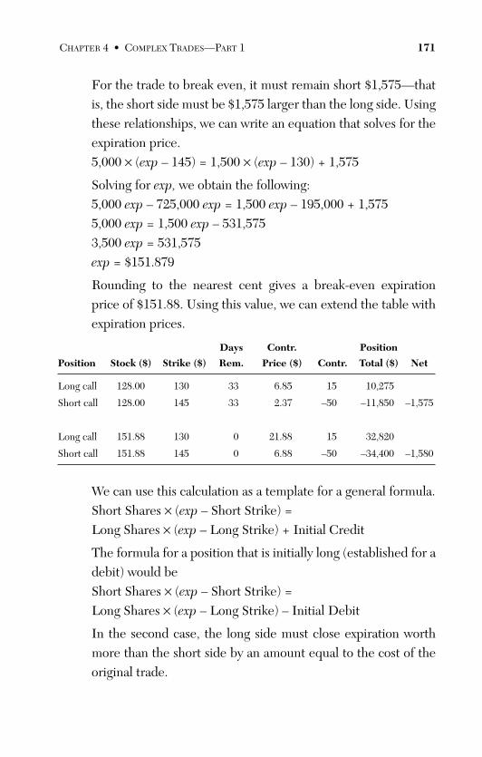
ptg
For the trade to break even, it must remain short $1,575—thatis, the short side must be $1,575 larger than the long side. Usingthese relationships, we can write an equation that solves for theexpiration price.5,000 × (exp – 145) = 1,500 × (exp – 130) + 1,575
Solving for exp, we obtain the following:5,000 exp – 725,000 exp = 1,500 exp – 195,000 + 1,5755,000 exp = 1,500 exp – 531,5753,500 exp = 531,575exp = $151.879
Rounding to the nearest cent gives a break-even expirationprice of $151.88. Using this value, we can extend the table withexpiration prices.
Days Contr. Position
Position Stock ($) Strike ($) Rem. Price ($) Contr. Total ($) Net
Long call 128.00 130 33 6.85 15 10,275
Short call 128.00 145 33 2.37 –50 –11,850 –1,575
Long call 151.88 130 0 21.88 15 32,820
Short call 151.88 145 0 6.88 –50 –34,400 –1,580
We can use this calculation as a template for a general formula.Short Shares × (exp – Short Strike) =Long Shares × (exp – Long Strike) + Initial Credit
The formula for a position that is initially long (established for adebit) would beShort Shares × (exp – Short Strike) =Long Shares × (exp – Long Strike) – Initial Debit
In the second case, the long side must close expiration worthmore than the short side by an amount equal to the cost of theoriginal trade.
CHAPTER 4 • COMPLEX TRADES—PART 1 171
From the Library of Melissa Wong
ptg
Summary
This chapter began with trades that span different strikes in thesame month and progressed to relatively complex trades crossingmultiple expiration dates and strike prices. We ended with a series ofproblems that compared different ratio structures with long and shortcomponents of different sizes.
Each of these structures will form an important springboard forthe next chapter, which addresses complex multipart trades spanningvarious combinations of strike price and month. These trades requirenimble and efficient execution and are generally found in the port-folios of private investors. Properly structured, they have the potentialto deliver substantial profits against a backdrop of well-managed risk.Unlike large institutions that distribute risk across many investmentvehicles and venues, private investors normally manage risk on atrade-by-trade basis. This dynamic significantly increases the value ofcomplex multipart trades because a portfolio can be structured usinga very small number of large positions.
172 THE OPTION TRADER’S WORKBOOK
From the Library of Melissa Wong
ptg
Complex Trades—Part 2
Until this point our focus has been structures composed of putsor calls spanning different strike prices and/or expiration dates. Thischapter extends those themes with more complex trades that containthree or more components. These structures, because of their com-plexity, offer additional advantages with regard to hedging and riskmanagement. For example, using the ratios of the previous chapter asa springboard, we can structure a position containing three strikesthat caps both the maximum gain and the maximum loss. These struc-tures, commonly referred to as “butterfly trades,” are quite popularamong private investors.
This chapter also builds on previous discussions with trades thatinvolve both puts and calls. Generally speaking, short put/call struc-tures generate profit from time decay while the corresponding longpositions bet on large underlying price changes. Stated differently,short put/call combinations succeed when implied volatility is over-priced, whereas the reverse structures, like all long positions, can beprofitable only if volatility is understated. These structures, known asstraddles and strangles, are the basis of more complex four-part tradesthat are both long and short, puts and calls. They can be built arounda large number of strike-price and expiration-date combinations.
In some sense this chapter represents a fork in the road becausethese trades have specific characteristics that make them difficult forlarge institutions and perfect for private investors and small invest-ment groups. Complex trades have many components and speed of
5
173
From the Library of Melissa Wong
ptg
execution is key to their success. Institutional investors placing verylarge trades containing thousands of contracts are unlikely to pursuesuch structures. Furthermore, bid-ask spreads represent a significantexpense for a multisided trade, and the associated costs double if theposition needs to be adjusted. The inefficiencies associated withunwinding and rebuilding complex positions amplifies the bid-askspread problem, which is further aggravated by very large trades.
Large institutions also take a different approach to hedging thanprivate investors because their portfolios are significantly larger andthey can spread risk across many different investments. Conversely,most private investors are sensitive to the loss from a single failedtrade, and it makes sense to build structures that are individuallyhedged. Trades that cap both the maximum gain and maximum losstend to deliver more stable profit over time. This dynamic allows pri-vate investors with relatively few investments to realize the same sta-ble return pattern as a large institution with an enormously diverseportfolio. In this regard, complex multipart trades can be thought ofas being more conservative than the more familiar calendar, vertical,and diagonal spreads, ratios, or simple long or short option positions.However, as with any complex device containing many moving parts,management and fine-tuning are key success factors. The exercises inthis chapter are designed to address this additional level of complex-ity. (All calculations for this chapter are based on a 1.5% risk-freeinterest rate.)
Butterfly Spreads (Problems #1–#8)
1. The following table depicts the three components of a typicallong butterfly spread. What is the maximum potential profit atexpiration? What is the maximum potential loss?
174 THE OPTION TRADER’S WORKBOOK
From the Library of Melissa Wong
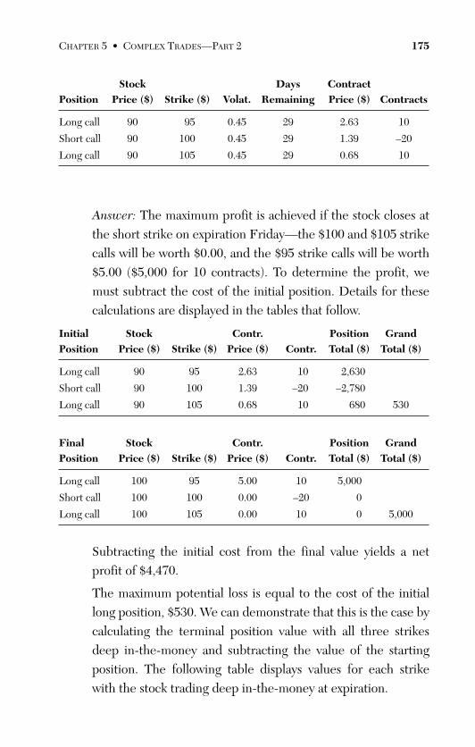
ptg
Stock Days ContractPosition Price ($) Strike ($) Volat. Remaining Price ($) Contracts
Long call 90 95 0.45 29 2.63 10
Short call 90 100 0.45 29 1.39 –20
Long call 90 105 0.45 29 0.68 10
Answer: The maximum profit is achieved if the stock closes atthe short strike on expiration Friday—the $100 and $105 strikecalls will be worth $0.00, and the $95 strike calls will be worth$5.00 ($5,000 for 10 contracts). To determine the profit, wemust subtract the cost of the initial position. Details for thesecalculations are displayed in the tables that follow.
Initial Stock Contr. Position Grand Position Price ($) Strike ($) Price ($) Contr. Total ($) Total ($)
Long call 90 95 2.63 10 2,630
Short call 90 100 1.39 –20 –2,780
Long call 90 105 0.68 10 680 530
Final Stock Contr. Position Grand Position Price ($) Strike ($) Price ($) Contr. Total ($) Total ($)
Long call 100 95 5.00 10 5,000
Short call 100 100 0.00 –20 0
Long call 100 105 0.00 10 0 5,000
Subtracting the initial cost from the final value yields a netprofit of $4,470.
The maximum potential loss is equal to the cost of the initiallong position, $530. We can demonstrate that this is the case bycalculating the terminal position value with all three strikesdeep in-the-money and subtracting the value of the startingposition. The following table displays values for each strikewith the stock trading deep in-the-money at expiration.
CHAPTER 5 • COMPLEX TRADES—PART 2 175
From the Library of Melissa Wong
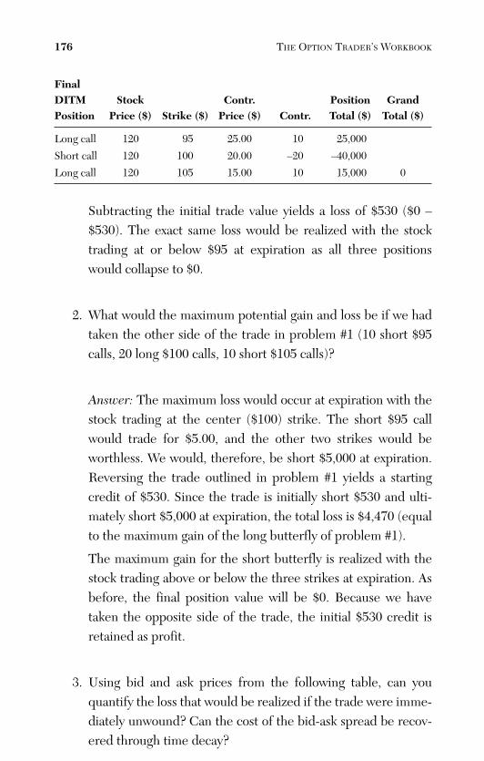
ptg
FinalDITM Stock Contr. Position Grand Position Price ($) Strike ($) Price ($) Contr. Total ($) Total ($)
Long call 120 95 25.00 10 25,000
Short call 120 100 20.00 –20 –40,000
Long call 120 105 15.00 10 15,000 0
Subtracting the initial trade value yields a loss of $530 ($0 –$530). The exact same loss would be realized with the stocktrading at or below $95 at expiration as all three positionswould collapse to $0.
2. What would the maximum potential gain and loss be if we hadtaken the other side of the trade in problem #1 (10 short $95calls, 20 long $100 calls, 10 short $105 calls)?
Answer: The maximum loss would occur at expiration with thestock trading at the center ($100) strike. The short $95 callwould trade for $5.00, and the other two strikes would beworthless. We would, therefore, be short $5,000 at expiration.Reversing the trade outlined in problem #1 yields a startingcredit of $530. Since the trade is initially short $530 and ulti-mately short $5,000 at expiration, the total loss is $4,470 (equalto the maximum gain of the long butterfly of problem #1).
The maximum gain for the short butterfly is realized with thestock trading above or below the three strikes at expiration. Asbefore, the final position value will be $0. Because we havetaken the opposite side of the trade, the initial $530 credit isretained as profit.
3. Using bid and ask prices from the following table, can youquantify the loss that would be realized if the trade were imme-diately unwound? Can the cost of the bid-ask spread be recov-ered through time decay?
176 THE OPTION TRADER’S WORKBOOK
From the Library of Melissa Wong
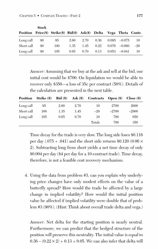
ptg
StockPosition Price($) Strike($) Bid($) Ask($) Delta Vega Theta Contr.
Long call 90 95 2.60 2.70 0.36 0.095 –0.075 10
Short call 90 100 1.35 1.45 0.22 0.076 –0.060 –20
Long call 90 105 0.65 0.70 0.13 0.053 –0.041 10
Answer: Assuming that we buy at the ask and sell at the bid, ourinitial cost would be $700. On liquidation we would be able torecover only $350—a loss of 35¢ per contract (50%). Details ofthe calculation are presented in the next table.
Position Strike ($) Bid ($) Ask ($) Contracts Open ($) Close ($)
Long call 95 2.60 2.70 10 2700 2600
Short call 100 1.35 1.45 –20 –2700 –2900
Long call 105 0.65 0.70 10 700 650
Totals 700 350
Time decay for the trade is very slow. The long side loses $0.116per day (.075 + .041) and the short side returns $0.120 (0.06 ×2). Subtracting long from short yields a net time decay of only$0.004 per day ($4 per day for a 10-contract trade). Time decay,therefore, is not a feasible cost recovery mechanism.
4. Using the data from problem #3, can you explain why underly-ing price changes have only modest effects on the value of abutterfly spread? How would the trade be affected by a largechange in implied volatility? How would the initial positionvalue be affected if implied volatility were double that of prob-lem #3 (90%). (Hint: Think about overall trade delta and vega.)
Answer: Net delta for the starting position is nearly neutral.Furthermore, we can predict that the hedged structure of theposition will preserve this neutrality. The initial value is equal to0.36 – (0.22 × 2) + 0.13 = 0.05. We can also infer that delta will
CHAPTER 5 • COMPLEX TRADES—PART 2 177
From the Library of Melissa Wong
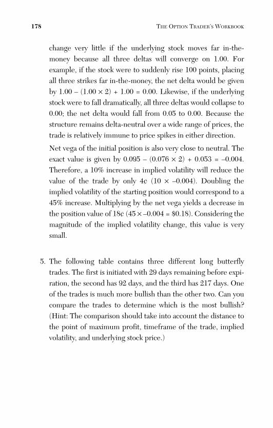
ptg
change very little if the underlying stock moves far in-the-money because all three deltas will converge on 1.00. Forexample, if the stock were to suddenly rise 100 points, placingall three strikes far in-the-money, the net delta would be givenby 1.00 – (1.00 × 2) + 1.00 = 0.00. Likewise, if the underlyingstock were to fall dramatically, all three deltas would collapse to0.00; the net delta would fall from 0.05 to 0.00. Because thestructure remains delta-neutral over a wide range of prices, thetrade is relatively immune to price spikes in either direction.
Net vega of the initial position is also very close to neutral. Theexact value is given by 0.095 – (0.076 × 2) + 0.053 = –0.004.Therefore, a 10% increase in implied volatility will reduce thevalue of the trade by only 4¢ (10 × –0.004). Doubling theimplied volatility of the starting position would correspond to a45% increase. Multiplying by the net vega yields a decrease inthe position value of 18¢ (45 × –0.004 = $0.18). Considering themagnitude of the implied volatility change, this value is verysmall.
5. The following table contains three different long butterflytrades. The first is initiated with 29 days remaining before expi-ration, the second has 92 days, and the third has 217 days. Oneof the trades is much more bullish than the other two. Can youcompare the trades to determine which is the most bullish?(Hint: The comparison should take into account the distance tothe point of maximum profit, timeframe of the trade, impliedvolatility, and underlying stock price.)
178 THE OPTION TRADER’S WORKBOOK
From the Library of Melissa Wong
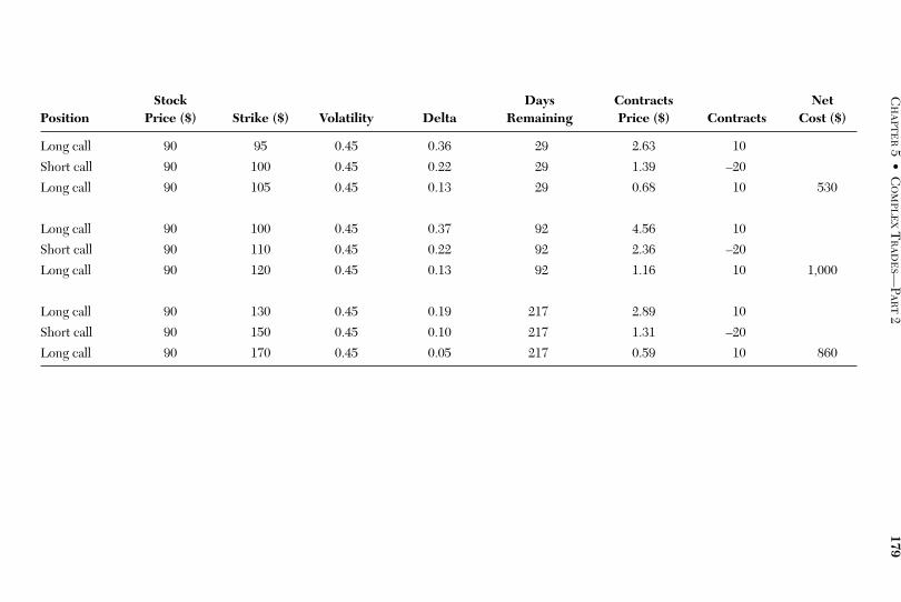
ptg
Stock Days Contracts Net Position Price ($) Strike ($) Volatility Delta Remaining Price ($) Contracts Cost ($)
Long call 90 95 0.45 0.36 29 2.63 10
Short call 90 100 0.45 0.22 29 1.39 –20
Long call 90 105 0.45 0.13 29 0.68 10 530
Long call 90 100 0.45 0.37 92 4.56 10
Short call 90 110 0.45 0.22 92 2.36 –20
Long call 90 120 0.45 0.13 92 1.16 10 1,000
Long call 90 130 0.45 0.19 217 2.89 10
Short call 90 150 0.45 0.10 217 1.31 –20
Long call 90 170 0.45 0.05 217 0.59 10 860
CH
APT
ER
5•
CO
MPL
EX
TR
AD
ES—
PA
RT
2179
From the Library of Melissa Wong
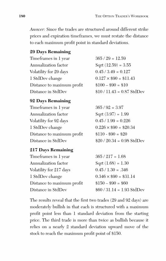
ptg
Answer: Since the trades are structured around different strikeprices and expiration timeframes, we must restate the distanceto each maximum profit point in standard deviations.
29 Days RemainingTimeframes in 1 year 365 / 29 = 12.59Annualization factor Sqrt (12.59) = 3.55Volatility for 29 days 0.45 / 3.49 = 0.1271 StdDev change 0.127 × $90 = $11.43Distance to maximum profit $100 – $90 = $10Distance in StdDev $10 / 11.43 = 0.87 StdDev
92 Days RemainingTimeframes in 1 year 365 / 92 = 3.97Annualization factor Sqrt (3.97) = 1.99Volatility for 92 days 0.45 / 1.99 = 0.2261 StdDev change 0.226 × $90 = $20.34Distance to maximum profit $110 - $90 = $20Distance in StdDev $20 / 20.34 = 0.98 StdDev
217 Days RemainingTimeframes in 1 year 365 / 217 = 1.68Annualization factor Sqrt (1.68) = 1.30Volatility for 217 days 0.45 / 1.30 = .3461 StdDev change 0.346 × $90 = $31.14Distance to maximum profit $150 – $90 = $60Distance in StdDev $60 / 31.14 = 1.93 StdDev
The results reveal that the first two trades (29 and 92 days) aremoderately bullish in that each is structured with a maximumprofit point less than 1 standard deviation from the startingprice. The third trade is more than twice as bullish because itrelies on a nearly 2 standard deviation upward move of thestock to reach the maximum profit point of $150.
180 THE OPTION TRADER’S WORKBOOK
From the Library of Melissa Wong
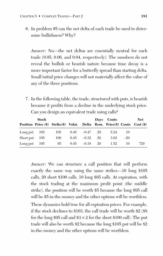
ptg
6. In problem #5 can the net delta of each trade be used to deter-mine bullishness? Why?
Answer: No—the net deltas are essentially neutral for eachtrade (0.05, 0.06, and 0.04, respectively). The numbers do notreveal the bullish or bearish nature because time decay is amore important factor for a butterfly spread than starting delta.Small initial price changes will not materially affect the value ofany of the three positions.
7. In the following table, the trade, structured with puts, is bearishbecause it profits from a decline in the underlying stock price.Can you design an equivalent trade using calls?
Stock Days Contr. NetPosition Price ($) Strike($) Volat. Delta Rem. Price($) Contr. Cost ($)
Long put 105 105 0.45 –0.47 29 5.24 10
Short put 105 100 0.45 –0.32 29 3.02 –20
Long put 105 95 0.45 –0.19 29 1.52 10 720
Answer: We can structure a call position that will performexactly the same way using the same strikes—10 long $105calls, 20 short $100 calls, 10 long $95 calls. At expiration, withthe stock trading at the maximum profit point (the middlestrike), the position will be worth $5 because the long $95 callwill be $5 in-the-money and the other options will be worthless.
These dynamics hold true for all expiration prices. For example,if the stock declines to $103, the call trade will be worth $2 ($8for the long $95 call and $3 × 2 for the short $100 call). The puttrade will also be worth $2 because the long $105 put will be $2in-the-money and the other options will be worthless.
CHAPTER 5 • COMPLEX TRADES—PART 2 181
From the Library of Melissa Wong
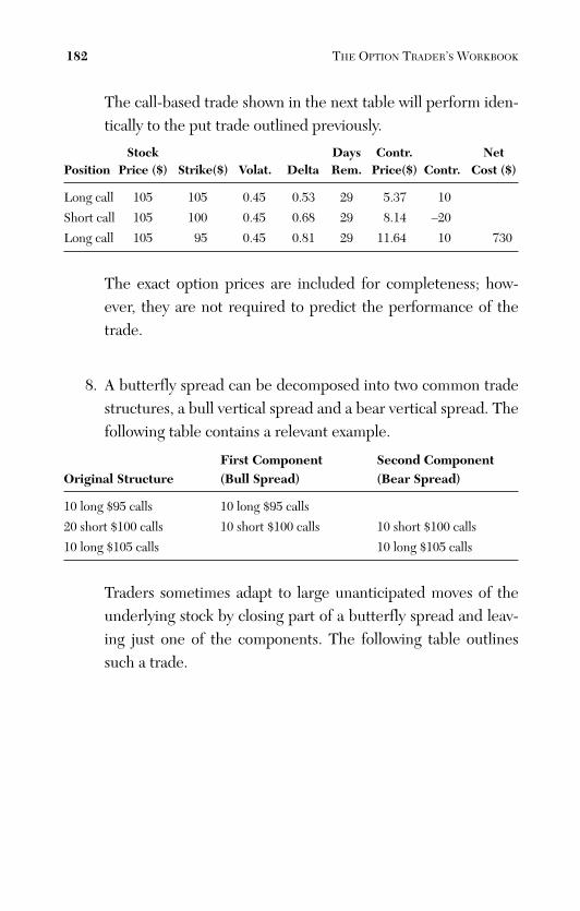
ptg
The call-based trade shown in the next table will perform iden-tically to the put trade outlined previously.
Stock Days Contr. NetPosition Price ($) Strike($) Volat. Delta Rem. Price($) Contr. Cost ($)
Long call 105 105 0.45 0.53 29 5.37 10
Short call 105 100 0.45 0.68 29 8.14 –20
Long call 105 95 0.45 0.81 29 11.64 10 730
The exact option prices are included for completeness; how-ever, they are not required to predict the performance of thetrade.
8. A butterfly spread can be decomposed into two common tradestructures, a bull vertical spread and a bear vertical spread. Thefollowing table contains a relevant example.
First Component Second Component Original Structure (Bull Spread) (Bear Spread)
10 long $95 calls 10 long $95 calls
20 short $100 calls 10 short $100 calls 10 short $100 calls
10 long $105 calls 10 long $105 calls
Traders sometimes adapt to large unanticipated moves of theunderlying stock by closing part of a butterfly spread and leav-ing just one of the components. The following table outlinessuch a trade.
182 THE OPTION TRADER’S WORKBOOK
From the Library of Melissa Wong
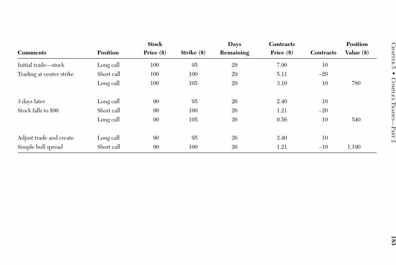
ptg
Stock Days Contracts PositionComments Position Price ($) Strike ($) Remaining Price ($) Contracts Value ($)
Initial trade—stock Long call 100 95 29 7.90 10
Trading at center strike Short call 100 100 29 5.11 –20
Long call 100 105 29 3.10 10 780
3 days later Long call 90 95 26 2.40 10
Stock falls to $90 Short call 90 100 26 1.21 –20
Long call 90 105 26 0.56 10 540
Adjust trade and create Long call 90 95 26 2.40 10
Simple bull spread Short call 90 100 26 1.21 –10 1,190
CH
APT
ER
5•
CO
MPL
EX
TR
AD
ES—
PA
RT
2183
From the Library of Melissa Wong
ptg
What is the maximum potential profit that can be achieved ifthe stock changes direction and rallies before expiration? Whatis the maximum potential loss? Does the new structure have anadvantage that would make the cost of the position adjustmentworthwhile?
Answer: After 3 days we corrected the position by repurchasing10 short $100 calls for $1.21 and selling 10 long $105 calls for$0.56 (total cost is $0.65 or $650 for 10 contracts). It is temptingto think of the adjustment as representing a $1.36 profitbecause the original bear spread was short $2.01 ($5.11 –$3.10). However, this profit is offset by a $1.60 loss in the bullspread that was originally long $2.79 ($7.90 – $5.11) and is nowlong only $1.19 ($2.40 – $1.21).
At expiration, if the stock closes above $100, the position will beworth $5,000. Subtracting the initial trade cost ($780) and theadjustment cost ($650) leaves a profit of $3,570. If, however,the stock continues falling, we will lose both the initial invest-ment of $780 and the cost of the adjustment ($650). Total lossfor the trade will then be $1,430.
It would appear that the adjustment adds no value because itreduces the maximum profit and increases the maximum loss.However, the original trade generates its maximum profit onlyif the stock closes at $100. Conversely, the adjusted trade gen-erates its maximum profit at any point above $100. This struc-ture has advantages for stocks that trade erratically because itgenerates the maximum profit at all price points above $100.
184 THE OPTION TRADER’S WORKBOOK
From the Library of Melissa Wong
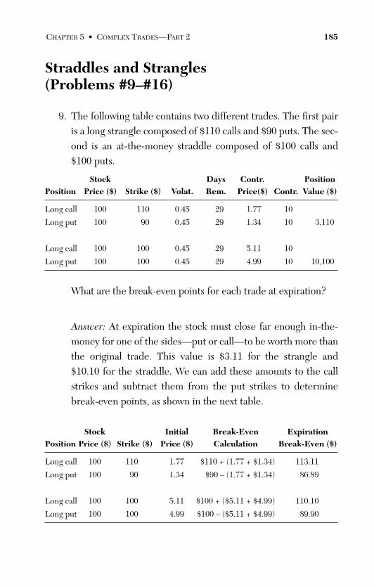
ptg
Straddles and Strangles (Problems #9–#16)
9. The following table contains two different trades. The first pairis a long strangle composed of $110 calls and $90 puts. The sec-ond is an at-the-money straddle composed of $100 calls and$100 puts.
Stock Days Contr. PositionPosition Price ($) Strike ($) Volat. Rem. Price($) Contr. Value ($)
Long call 100 110 0.45 29 1.77 10
Long put 100 90 0.45 29 1.34 10 3,110
Long call 100 100 0.45 29 5.11 10
Long put 100 100 0.45 29 4.99 10 10,100
What are the break-even points for each trade at expiration?
Answer: At expiration the stock must close far enough in-the-money for one of the sides—put or call—to be worth more thanthe original trade. This value is $3.11 for the strangle and$10.10 for the straddle. We can add these amounts to the callstrikes and subtract them from the put strikes to determinebreak-even points, as shown in the next table.
Stock Initial Break-Even ExpirationPosition Price ($) Strike ($) Price ($) Calculation Break-Even ($)
Long call 100 110 1.77 $110 + (1.77 + $1.34) 113.11
Long put 100 90 1.34 $90 – (1.77 + $1.34) 86.89
Long call 100 100 5.11 $100 + ($5.11 + $4.99) 110.10
Long put 100 100 4.99 $100 – ($5.11 + $4.99) 89.90
CHAPTER 5 • COMPLEX TRADES—PART 2 185
From the Library of Melissa Wong
ptg
10. What is the profit or loss for each of the trades outlined in prob-lem #9 with the stock trading at $105, $110, and $115 at expira-tion?
Answer: The following table contains three pairs of results;each contains expiration prices and profit/loss values for bothtrades.
Stock Contr. Initial Exp. Profit/Position Price ($) Strike ($) Price ($) Contr. Value($) Value($) Loss
Long call 105 110 0.00 10
Long put 105 90 0.00 10 3,110 0 –100%
Long call 105 100 5.00 10
Long put 105 100 0.00 10 10,100 5,000 –50%
Long call 110 110 0.00 10
Long put 110 90 0.00 10 3,110 0 –100%
Long call 110 100 10.00 10
Long put 110 100 0.00 10 10,100 10,000 0%
Long call 115 110 5.00 10
Long put 115 90 0.00 10 3,110 5,000 61%
Long call 115 100 15.00 10
Long put 115 100 0.00 10 10,100 15,000 49%
11. The following table is based on the first trade of the precedingtwo problems. It contains three pairs of entries. The first pair isthe initial trade; the second and third are the same trade after 4days and at expiration. Without knowing exact option prices forthe second pair, can you predict which is most profitable?
186 THE OPTION TRADER’S WORKBOOK
From the Library of Melissa Wong
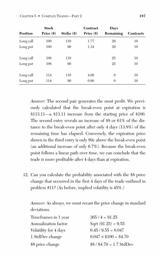
ptg
Stock Contract Days Position Price ($) Strike ($) Price ($) Remaining Contracts
Long call 100 110 1.77 29 10
Long put 100 90 1.34 29 10
Long call 108 110 25 10
Long put 108 90 25 10
Long call 114 110 4.00 0 10
Long put 114 90 0.00 0 10
Answer: The second pair generates the most profit. We previ-ously calculated that the break-even point at expiration is$113.11—a $13.11 increase from the starting price of $100.The second entry reveals an increase of $8 or 61% of the dis-tance to the break-even point after only 4 days (13.8%) of theremaining time has elapsed. Conversely, the expiration priceshown in the third entry is only 89¢ above the break-even point(an additional increase of only 6.7%). Because the break-evenpoint follows a linear path over time, we can conclude that thetrade is more profitable after 4 days than at expiration.
12. Can you calculate the probability associated with the $8 pricechange that occurred in the first 4 days of the trade outlined inproblem #11? (As before, implied volatility is 45%.)
Answer: As always, we must recast the price change in standarddeviations.
Timeframes in 1 year 365 / 4 = 91.25Annualization factor Sqrt (91.25) = 9.55Volatility for 4 days 0.45 / 9.55 = 0.0471 StdDev change 0.047 × $100 = $4.70
$8 price change $8 / $4.70 = 1.7 StdDev
CHAPTER 5 • COMPLEX TRADES—PART 2 187
From the Library of Melissa Wong
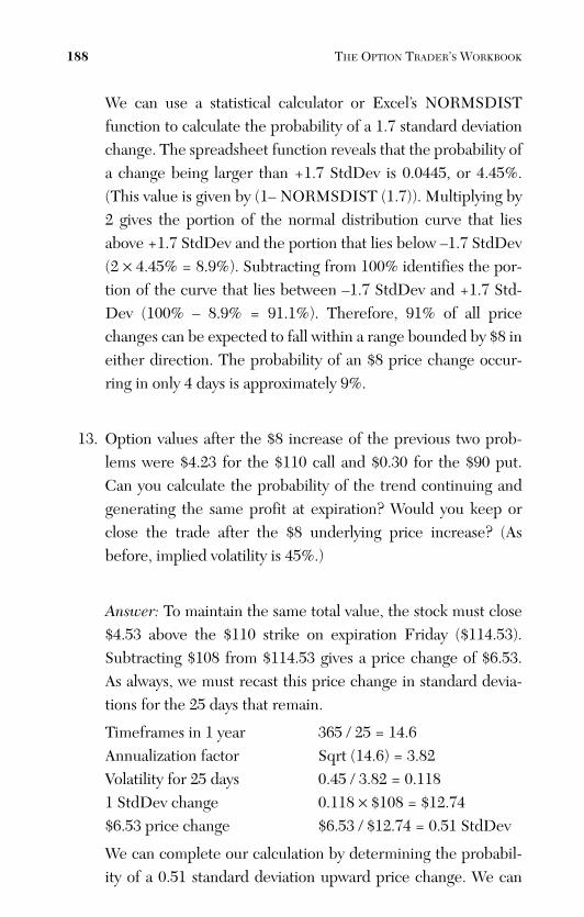
ptg
We can use a statistical calculator or Excel’s NORMSDISTfunction to calculate the probability of a 1.7 standard deviationchange. The spreadsheet function reveals that the probability ofa change being larger than +1.7 StdDev is 0.0445, or 4.45%.(This value is given by (1– NORMSDIST (1.7)). Multiplying by2 gives the portion of the normal distribution curve that liesabove +1.7 StdDev and the portion that lies below –1.7 StdDev(2 × 4.45% = 8.9%). Subtracting from 100% identifies the por-tion of the curve that lies between –1.7 StdDev and +1.7 Std-Dev (100% – 8.9% = 91.1%). Therefore, 91% of all pricechanges can be expected to fall within a range bounded by $8 ineither direction. The probability of an $8 price change occur-ring in only 4 days is approximately 9%.
13. Option values after the $8 increase of the previous two prob-lems were $4.23 for the $110 call and $0.30 for the $90 put.Can you calculate the probability of the trend continuing andgenerating the same profit at expiration? Would you keep orclose the trade after the $8 underlying price increase? (Asbefore, implied volatility is 45%.)
Answer: To maintain the same total value, the stock must close$4.53 above the $110 strike on expiration Friday ($114.53).Subtracting $108 from $114.53 gives a price change of $6.53.As always, we must recast this price change in standard devia-tions for the 25 days that remain.
Timeframes in 1 year 365 / 25 = 14.6Annualization factor Sqrt (14.6) = 3.82Volatility for 25 days 0.45 / 3.82 = 0.1181 StdDev change 0.118 × $108 = $12.74$6.53 price change $6.53 / $12.74 = 0.51 StdDev
We can complete our calculation by determining the probabil-ity of a 0.51 standard deviation upward price change. We can
188 THE OPTION TRADER’S WORKBOOK
From the Library of Melissa Wong
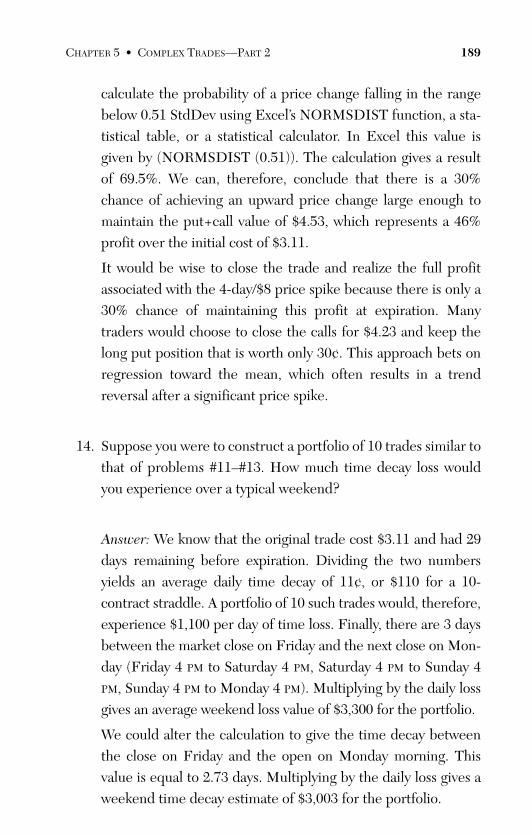
ptg
calculate the probability of a price change falling in the rangebelow 0.51 StdDev using Excel’s NORMSDIST function, a sta-tistical table, or a statistical calculator. In Excel this value isgiven by (NORMSDIST (0.51)). The calculation gives a resultof 69.5%. We can, therefore, conclude that there is a 30%chance of achieving an upward price change large enough tomaintain the put+call value of $4.53, which represents a 46%profit over the initial cost of $3.11.
It would be wise to close the trade and realize the full profitassociated with the 4-day/$8 price spike because there is only a30% chance of maintaining this profit at expiration. Manytraders would choose to close the calls for $4.23 and keep thelong put position that is worth only 30¢. This approach bets onregression toward the mean, which often results in a trendreversal after a significant price spike.
14. Suppose you were to construct a portfolio of 10 trades similar tothat of problems #11–#13. How much time decay loss wouldyou experience over a typical weekend?
Answer: We know that the original trade cost $3.11 and had 29days remaining before expiration. Dividing the two numbersyields an average daily time decay of 11¢, or $110 for a 10-contract straddle. A portfolio of 10 such trades would, therefore,experience $1,100 per day of time loss. Finally, there are 3 daysbetween the market close on Friday and the next close on Mon-day (Friday 4 PM to Saturday 4 PM, Saturday 4 PM to Sunday 4PM, Sunday 4 PM to Monday 4 PM). Multiplying by the daily lossgives an average weekend loss value of $3,300 for the portfolio.
We could alter the calculation to give the time decay betweenthe close on Friday and the open on Monday morning. Thisvalue is equal to 2.73 days. Multiplying by the daily loss gives aweekend time decay estimate of $3,003 for the portfolio.
CHAPTER 5 • COMPLEX TRADES—PART 2 189
From the Library of Melissa Wong
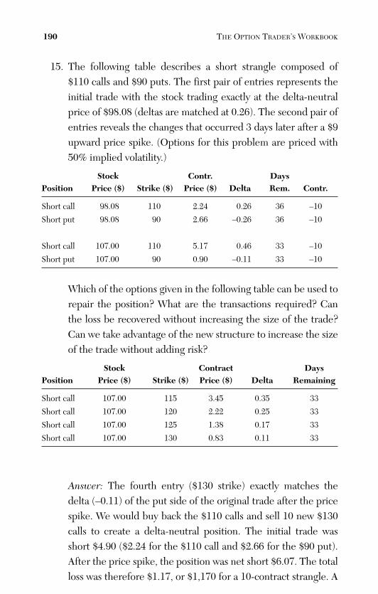
ptg
15. The following table describes a short strangle composed of$110 calls and $90 puts. The first pair of entries represents theinitial trade with the stock trading exactly at the delta-neutralprice of $98.08 (deltas are matched at 0.26). The second pair ofentries reveals the changes that occurred 3 days later after a $9upward price spike. (Options for this problem are priced with50% implied volatility.)
Stock Contr. DaysPosition Price ($) Strike ($) Price ($) Delta Rem. Contr.
Short call 98.08 110 2.24 0.26 36 –10
Short put 98.08 90 2.66 –0.26 36 –10
Short call 107.00 110 5.17 0.46 33 –10
Short put 107.00 90 0.90 –0.11 33 –10
Which of the options given in the following table can be used torepair the position? What are the transactions required? Canthe loss be recovered without increasing the size of the trade?Can we take advantage of the new structure to increase the sizeof the trade without adding risk?
Stock Contract DaysPosition Price ($) Strike ($) Price ($) Delta Remaining
Short call 107.00 115 3.45 0.35 33
Short call 107.00 120 2.22 0.25 33
Short call 107.00 125 1.38 0.17 33
Short call 107.00 130 0.83 0.11 33
Answer: The fourth entry ($130 strike) exactly matches thedelta (–0.11) of the put side of the original trade after the pricespike. We would buy back the $110 calls and sell 10 new $130calls to create a delta-neutral position. The initial trade wasshort $4.90 ($2.24 for the $110 call and $2.66 for the $90 put).After the price spike, the position was net short $6.07. The totalloss was therefore $1.17, or $1,170 for a 10-contract strangle. A
190 THE OPTION TRADER’S WORKBOOK
From the Library of Melissa Wong
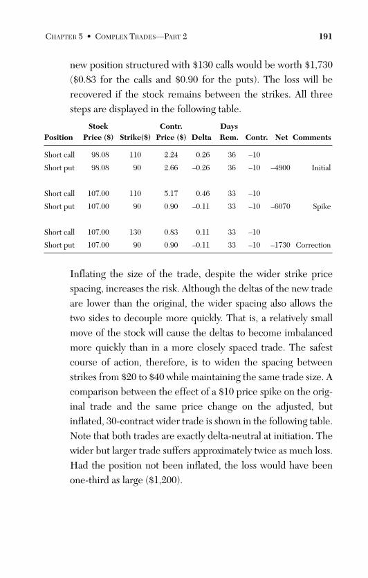
ptg
new position structured with $130 calls would be worth $1,730($0.83 for the calls and $0.90 for the puts). The loss will berecovered if the stock remains between the strikes. All threesteps are displayed in the following table.
Stock Contr. DaysPosition Price ($) Strike($) Price ($) Delta Rem. Contr. Net Comments
Short call 98.08 110 2.24 0.26 36 –10
Short put 98.08 90 2.66 –0.26 36 –10 –4900 Initial
Short call 107.00 110 5.17 0.46 33 –10
Short put 107.00 90 0.90 –0.11 33 –10 –6070 Spike
Short call 107.00 130 0.83 0.11 33 –10
Short put 107.00 90 0.90 –0.11 33 –10 –1730 Correction
Inflating the size of the trade, despite the wider strike pricespacing, increases the risk. Although the deltas of the new tradeare lower than the original, the wider spacing also allows thetwo sides to decouple more quickly. That is, a relatively smallmove of the stock will cause the deltas to become imbalancedmore quickly than in a more closely spaced trade. The safestcourse of action, therefore, is to widen the spacing betweenstrikes from $20 to $40 while maintaining the same trade size. Acomparison between the effect of a $10 price spike on the orig-inal trade and the same price change on the adjusted, butinflated, 30-contract wider trade is shown in the following table.Note that both trades are exactly delta-neutral at initiation. Thewider but larger trade suffers approximately twice as much loss.Had the position not been inflated, the loss would have beenone-third as large ($1,200).
CHAPTER 5 • COMPLEX TRADES—PART 2 191
From the Library of Melissa Wong
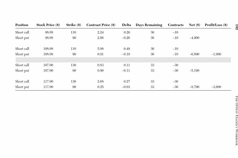
ptg
Position Stock Price ($) Strike ($) Contract Price ($) Delta Days Remaining Contracts Net ($) Profit/Loss ($)
Short call 98.08 110 2.24 0.26 36 –10
Short put 98.08 90 2.66 –0.26 36 –10 –4,900
Short call 108.08 110 5.98 0.49 36 –10
Short put 108.08 90 0.91 –0.10 36 –10 –6,890 –1,990
Short call 107.00 130 0.83 0.11 33 –30
Short put 107.00 90 0.90 –0.11 33 –30 –5,190
Short call 117.00 130 2.68 0.27 33 –30
Short put 117.00 90 0.25 –0.03 33 –30 –8,790 –3,600
192T
HE
OPT
ION
TR
AD
ER’S
WO
RK
BO
OK
From the Library of Melissa Wong
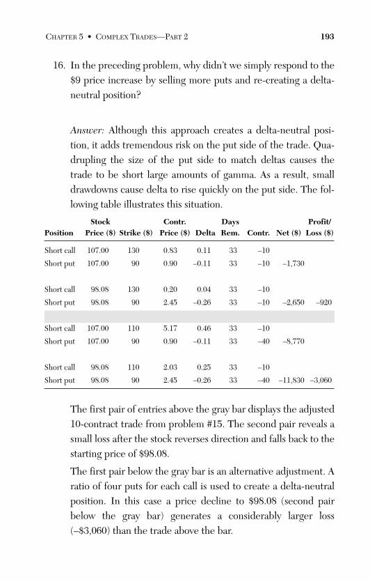
ptg
16. In the preceding problem, why didn’t we simply respond to the$9 price increase by selling more puts and re-creating a delta-neutral position?
Answer: Although this approach creates a delta-neutral posi-tion, it adds tremendous risk on the put side of the trade. Qua-drupling the size of the put side to match deltas causes thetrade to be short large amounts of gamma. As a result, smalldrawdowns cause delta to rise quickly on the put side. The fol-lowing table illustrates this situation.
Stock Contr. Days Profit/Position Price ($) Strike ($) Price ($) Delta Rem. Contr. Net ($) Loss ($)
Short call 107.00 130 0.83 0.11 33 –10
Short put 107.00 90 0.90 –0.11 33 –10 –1,730
Short call 98.08 130 0.20 0.04 33 –10
Short put 98.08 90 2.45 –0.26 33 –10 –2,650 –920
Short call 107.00 110 5.17 0.46 33 –10
Short put 107.00 90 0.90 –0.11 33 –40 –8,770
Short call 98.08 110 2.03 0.25 33 –10
Short put 98.08 90 2.45 –0.26 33 –40 –11,830 –3,060
The first pair of entries above the gray bar displays the adjusted10-contract trade from problem #15. The second pair reveals asmall loss after the stock reverses direction and falls back to thestarting price of $98.08.
The first pair below the gray bar is an alternative adjustment. Aratio of four puts for each call is used to create a delta-neutralposition. In this case a price decline to $98.08 (second pairbelow the gray bar) generates a considerably larger loss(–$3,060) than the trade above the bar.
CHAPTER 5 • COMPLEX TRADES—PART 2 193
From the Library of Melissa Wong
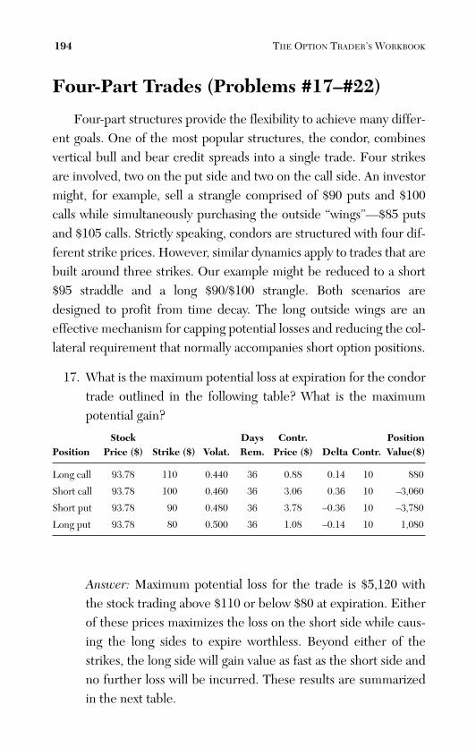
ptg
Four-Part Trades (Problems #17–#22)
Four-part structures provide the flexibility to achieve many differ-ent goals. One of the most popular structures, the condor, combinesvertical bull and bear credit spreads into a single trade. Four strikesare involved, two on the put side and two on the call side. An investormight, for example, sell a strangle comprised of $90 puts and $100calls while simultaneously purchasing the outside “wings”—$85 putsand $105 calls. Strictly speaking, condors are structured with four dif-ferent strike prices. However, similar dynamics apply to trades that arebuilt around three strikes. Our example might be reduced to a short$95 straddle and a long $90/$100 strangle. Both scenarios aredesigned to profit from time decay. The long outside wings are aneffective mechanism for capping potential losses and reducing the col-lateral requirement that normally accompanies short option positions.
17. What is the maximum potential loss at expiration for the condortrade outlined in the following table? What is the maximumpotential gain?
Stock Days Contr. PositionPosition Price ($) Strike ($) Volat. Rem. Price ($) Delta Contr. Value($)
Long call 93.78 110 0.440 36 0.88 0.14 10 880
Short call 93.78 100 0.460 36 3.06 0.36 10 –3,060
Short put 93.78 90 0.480 36 3.78 –0.36 10 –3,780
Long put 93.78 80 0.500 36 1.08 –0.14 10 1,080
Answer: Maximum potential loss for the trade is $5,120 withthe stock trading above $110 or below $80 at expiration. Eitherof these prices maximizes the loss on the short side while caus-ing the long sides to expire worthless. Beyond either of thestrikes, the long side will gain value as fast as the short side andno further loss will be incurred. These results are summarizedin the next table.
194 THE OPTION TRADER’S WORKBOOK
From the Library of Melissa Wong
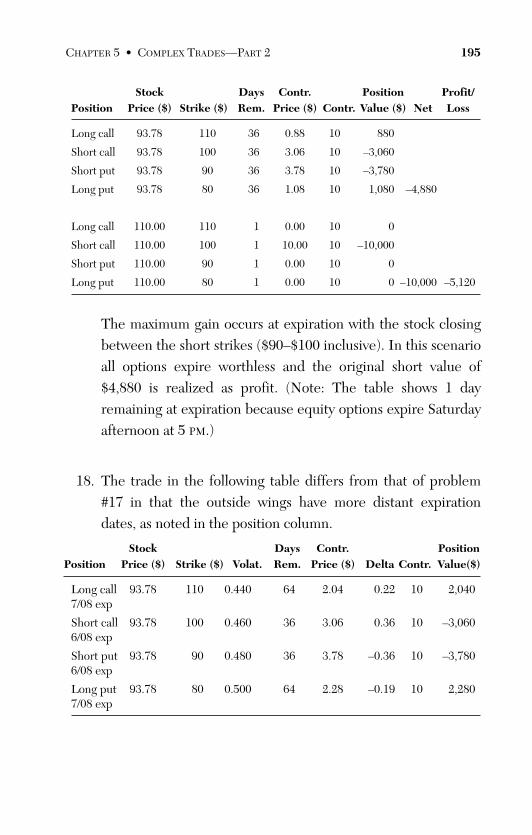
ptg
Stock Days Contr. Position Profit/Position Price ($) Strike ($) Rem. Price ($) Contr. Value ($) Net Loss
Long call 93.78 110 36 0.88 10 880
Short call 93.78 100 36 3.06 10 –3,060
Short put 93.78 90 36 3.78 10 –3,780
Long put 93.78 80 36 1.08 10 1,080 –4,880
Long call 110.00 110 1 0.00 10 0
Short call 110.00 100 1 10.00 10 –10,000
Short put 110.00 90 1 0.00 10 0
Long put 110.00 80 1 0.00 10 0 –10,000 –5,120
The maximum gain occurs at expiration with the stock closingbetween the short strikes ($90–$100 inclusive). In this scenarioall options expire worthless and the original short value of$4,880 is realized as profit. (Note: The table shows 1 dayremaining at expiration because equity options expire Saturdayafternoon at 5 PM.)
18. The trade in the following table differs from that of problem#17 in that the outside wings have more distant expirationdates, as noted in the position column.
Stock Days Contr. PositionPosition Price ($) Strike ($) Volat. Rem. Price ($) Delta Contr. Value($)
Long call 93.78 110 0.440 64 2.04 0.22 10 2,0407/08 exp
Short call 93.78 100 0.460 36 3.06 0.36 10 –3,0606/08 exp
Short put 93.78 90 0.480 36 3.78 –0.36 10 –3,7806/08 exp
Long put 93.78 80 0.500 64 2.28 –0.19 10 2,2807/08 exp
CHAPTER 5 • COMPLEX TRADES—PART 2 195
From the Library of Melissa Wong
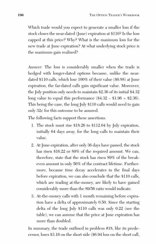
ptg
Which trade would you expect to generate a smaller loss if thestock closes the near-dated (June) expiration at $110? Is the losscapped at this price? Why? What is the maximum loss for thenew trade at June expiration? At what underlying stock price isthe maximum gain realized?
Answer: The loss is considerably smaller when the trade ishedged with longer-dated options because, unlike the near-dated $110 calls, which lose 100% of their value ($0.88) at Juneexpiration, the far-dated calls gain significant value. Moreover,the July position only needs to maintain $2.36 of its initial $4.32long value to equal this performance ($4.32 – $1.96 = $2.36).This being the case, the long July $110 calls would need to gainonly 32¢ for this outcome to be assured.
The following facts support these assertions.
1. The stock must rise $18.26 to $112.04 by July expiration,initially 64 days away, for the long calls to maintain theirvalue.
2. At June expiration, after only 36 days have passed, the stockhas risen $16.22 or 89% of the required amount. We can,therefore, state that the stock has risen 89% of the break-even amount in only 56% of the contract lifetime. Further-more, because time decay accelerates in the final daysbefore expiration, we can also conclude that the $110 calls,which are trading at-the-money, are likely to have gainedconsiderably more than the 89/56 ratio would indicate.
3. At-the-money calls with 1 month remaining before expira-tion have a delta of approximately 0.50. Since the startingdelta of the long July $110 calls was only 0.22 (see thetable), we can assume that the price at June expiration hasmore than doubled.
In summary, the trade outlined in problem #18, like its prede-cessor, loses $3.16 on the short side ($6.94 loss on the short call,
196 THE OPTION TRADER’S WORKBOOK
From the Library of Melissa Wong
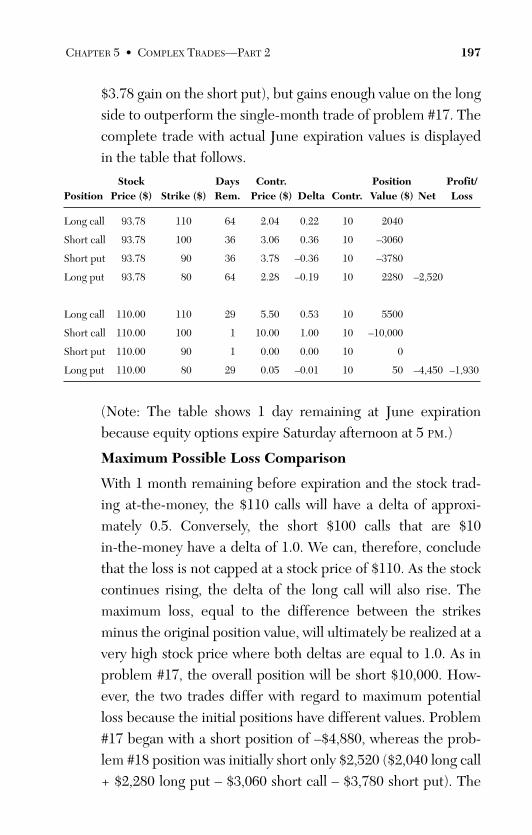
ptg
$3.78 gain on the short put), but gains enough value on the longside to outperform the single-month trade of problem #17. Thecomplete trade with actual June expiration values is displayedin the table that follows.
Stock Days Contr. Position Profit/Position Price ($) Strike ($) Rem. Price ($) Delta Contr. Value ($) Net Loss
Long call 93.78 110 64 2.04 0.22 10 2040
Short call 93.78 100 36 3.06 0.36 10 –3060
Short put 93.78 90 36 3.78 –0.36 10 –3780
Long put 93.78 80 64 2.28 –0.19 10 2280 –2,520
Long call 110.00 110 29 5.50 0.53 10 5500
Short call 110.00 100 1 10.00 1.00 10 –10,000
Short put 110.00 90 1 0.00 0.00 10 0
Long put 110.00 80 29 0.05 –0.01 10 50 –4,450 –1,930
(Note: The table shows 1 day remaining at June expirationbecause equity options expire Saturday afternoon at 5 PM.)
Maximum Possible Loss Comparison
With 1 month remaining before expiration and the stock trad-ing at-the-money, the $110 calls will have a delta of approxi-mately 0.5. Conversely, the short $100 calls that are $10in-the-money have a delta of 1.0. We can, therefore, concludethat the loss is not capped at a stock price of $110. As the stockcontinues rising, the delta of the long call will also rise. Themaximum loss, equal to the difference between the strikesminus the original position value, will ultimately be realized at avery high stock price where both deltas are equal to 1.0. As inproblem #17, the overall position will be short $10,000. How-ever, the two trades differ with regard to maximum potentialloss because the initial positions have different values. Problem#17 began with a short position of –$4,880, whereas the prob-lem #18 position was initially short only $2,520 ($2,040 long call+ $2,280 long put – $3,060 short call – $3,780 short put). The
CHAPTER 5 • COMPLEX TRADES—PART 2 197
From the Library of Melissa Wong
ptg
maximum possible loss at June expiration for the problem #18trade is, therefore, larger by $2,360 ($5,120 + $2,360 = $7,480).
Maximum Gain Point
At June expiration, the maximum gain will be realized with thestock trading at one of the short strikes because these pricepoints maximize the value of the long straddle while still caus-ing the short side to expire worthless. Beyond one of the insidestrikes, the short put or call will gain value with a delta of 1.0,and the long side will gain at a lower rate. We know from basicpricing theory that a $10 out-of-the-money call will always beworth more than a $10 out-of-the-money put (assuming thatother parameters such as remaining time, implied volatility, andrisk-free interest are identical). We can conclude, therefore,that the largest position value is achieved at June expirationwith the stock trading at the $100 short call strike. Because thisprice point falls below the line that extends from the startingprice ($93.78) to the expiration break-even point ($112.04), thelong calls will definitely have lost some value. This loss, in addi-tion to the loss from the long puts, must be subtracted from thegain on the short side. Exact values are displayed in the nexttable for completeness.
Stock Days Contr. Position Profit/Position Price ($) Strike ($) Rem. Price ($) Delta Contr. Value ($) Net Loss
Long call 93.78 110 64 2.04 0.22 10 2040
Short call 93.78 100 36 3.06 0.36 10 –3060
Short put 93.78 90 36 3.78 –0.36 10 –3780
Long put 93.78 80 64 2.28 –0.19 10 2280 –2,520
Long call 100.00 110 29 1.68 0.24 10 1680
Short call 100.00 100 1 0.00 0.78 10 0
Short put 100.00 90 1 0.00 0.00 10 0
Long put 100.00 80 29 0.30 –0.05 10 300 1,980 4,500
198 THE OPTION TRADER’S WORKBOOK
From the Library of Melissa Wong
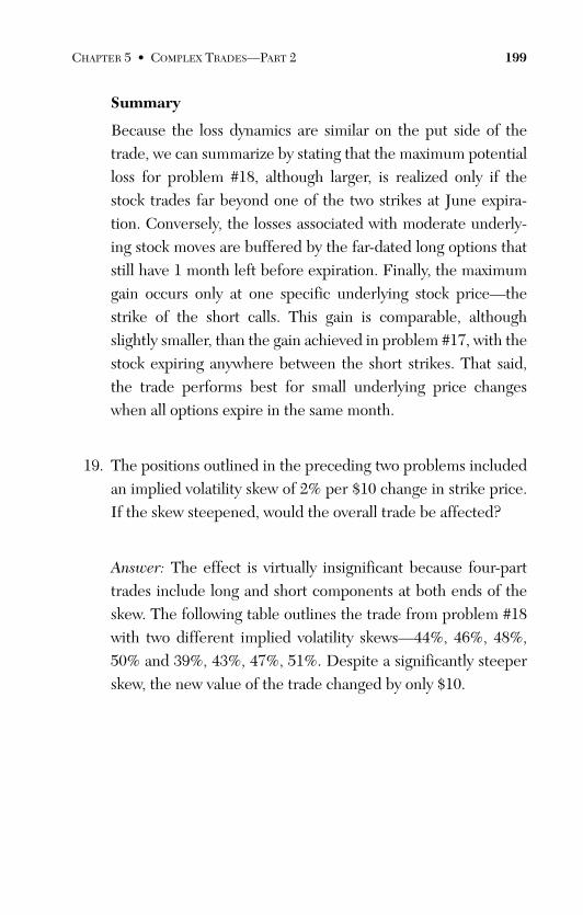
ptg
Summary
Because the loss dynamics are similar on the put side of thetrade, we can summarize by stating that the maximum potentialloss for problem #18, although larger, is realized only if thestock trades far beyond one of the two strikes at June expira-tion. Conversely, the losses associated with moderate underly-ing stock moves are buffered by the far-dated long options thatstill have 1 month left before expiration. Finally, the maximumgain occurs only at one specific underlying stock price—thestrike of the short calls. This gain is comparable, althoughslightly smaller, than the gain achieved in problem #17, with thestock expiring anywhere between the short strikes. That said,the trade performs best for small underlying price changeswhen all options expire in the same month.
19. The positions outlined in the preceding two problems includedan implied volatility skew of 2% per $10 change in strike price.If the skew steepened, would the overall trade be affected?
Answer: The effect is virtually insignificant because four-parttrades include long and short components at both ends of theskew. The following table outlines the trade from problem #18with two different implied volatility skews—44%, 46%, 48%,50% and 39%, 43%, 47%, 51%. Despite a significantly steeperskew, the new value of the trade changed by only $10.
CHAPTER 5 • COMPLEX TRADES—PART 2 199
From the Library of Melissa Wong
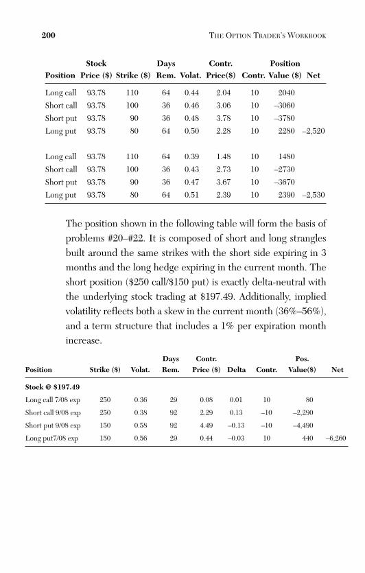
ptg
Stock Days Contr. PositionPosition Price ($) Strike ($) Rem. Volat. Price($) Contr. Value ($) Net
Long call 93.78 110 64 0.44 2.04 10 2040
Short call 93.78 100 36 0.46 3.06 10 –3060
Short put 93.78 90 36 0.48 3.78 10 –3780
Long put 93.78 80 64 0.50 2.28 10 2280 –2,520
Long call 93.78 110 64 0.39 1.48 10 1480
Short call 93.78 100 36 0.43 2.73 10 –2730
Short put 93.78 90 36 0.47 3.67 10 –3670
Long put 93.78 80 64 0.51 2.39 10 2390 –2,530
The position shown in the following table will form the basis ofproblems #20–#22. It is composed of short and long stranglesbuilt around the same strikes with the short side expiring in 3months and the long hedge expiring in the current month. Theshort position ($250 call/$150 put) is exactly delta-neutral withthe underlying stock trading at $197.49. Additionally, impliedvolatility reflects both a skew in the current month (36%–56%),and a term structure that includes a 1% per expiration monthincrease.
200 THE OPTION TRADER’S WORKBOOK
Days Contr. Pos.Position Strike ($) Volat. Rem. Price ($) Delta Contr. Value($) Net
Stock @ $197.49
Long call 7/08 exp 250 0.36 29 0.08 0.01 10 80
Short call 9/08 exp 250 0.38 92 2.29 0.13 –10 –2,290
Short put 9/08 exp 150 0.58 92 4.49 –0.13 –10 –4,490
Long put7/08 exp 150 0.56 29 0.44 –0.03 10 440 –6,260
From the Library of Melissa Wong
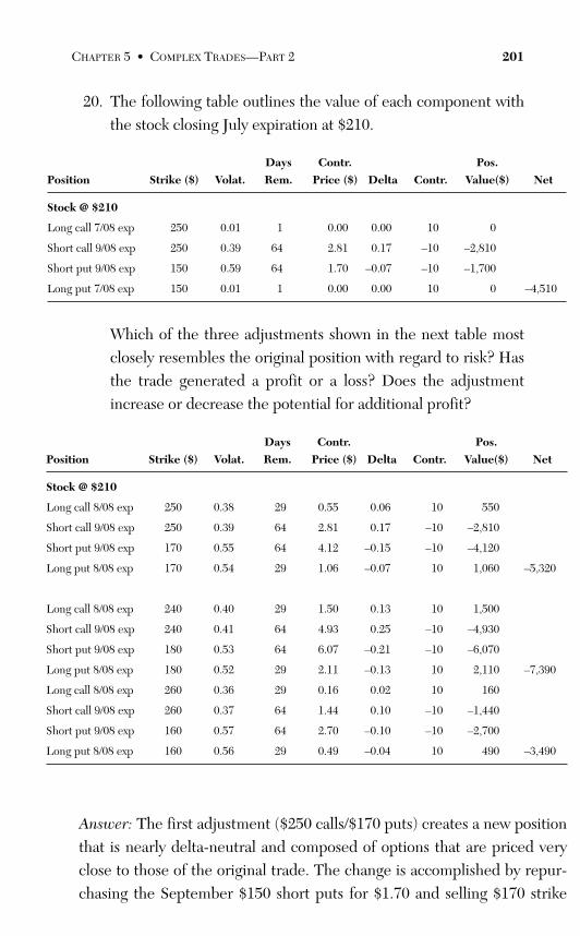
ptg
20. The following table outlines the value of each component withthe stock closing July expiration at $210.
CHAPTER 5 • COMPLEX TRADES—PART 2 201
Days Contr. Pos.Position Strike ($) Volat. Rem. Price ($) Delta Contr. Value($) Net
Stock @ $210
Long call 7/08 exp 250 0.01 1 0.00 0.00 10 0
Short call 9/08 exp 250 0.39 64 2.81 0.17 –10 –2,810
Short put 9/08 exp 150 0.59 64 1.70 –0.07 –10 –1,700
Long put 7/08 exp 150 0.01 1 0.00 0.00 10 0 –4,510
Which of the three adjustments shown in the next table mostclosely resembles the original position with regard to risk? Hasthe trade generated a profit or a loss? Does the adjustmentincrease or decrease the potential for additional profit?
Days Contr. Pos.Position Strike ($) Volat. Rem. Price ($) Delta Contr. Value($) Net
Stock @ $210
Long call 8/08 exp 250 0.38 29 0.55 0.06 10 550
Short call 9/08 exp 250 0.39 64 2.81 0.17 –10 –2,810
Short put 9/08 exp 170 0.55 64 4.12 –0.15 –10 –4,120
Long put 8/08 exp 170 0.54 29 1.06 –0.07 10 1,060 –5,320
Long call 8/08 exp 240 0.40 29 1.50 0.13 10 1,500
Short call 9/08 exp 240 0.41 64 4.93 0.25 –10 –4,930
Short put 9/08 exp 180 0.53 64 6.07 –0.21 –10 –6,070
Long put 8/08 exp 180 0.52 29 2.11 –0.13 10 2,110 –7,390
Long call 8/08 exp 260 0.36 29 0.16 0.02 10 160
Short call 9/08 exp 260 0.37 64 1.44 0.10 –10 –1,440
Short put 9/08 exp 160 0.57 64 2.70 –0.10 –10 –2,700
Long put 8/08 exp 160 0.56 29 0.49 –0.04 10 490 –3,490
Answer: The first adjustment ($250 calls/$170 puts) creates a new positionthat is nearly delta-neutral and composed of options that are priced veryclose to those of the original trade. The change is accomplished by repur-chasing the September $150 short puts for $1.70 and selling $170 strike
From the Library of Melissa Wong
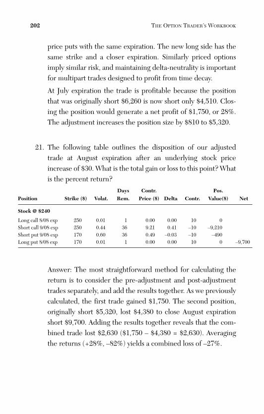
ptg
price puts with the same expiration. The new long side has thesame strike and a closer expiration. Similarly priced optionsimply similar risk, and maintaining delta-neutrality is importantfor multipart trades designed to profit from time decay.
At July expiration the trade is profitable because the positionthat was originally short $6,260 is now short only $4,510. Clos-ing the position would generate a net profit of $1,750, or 28%.The adjustment increases the position size by $810 to $5,320.
21. The following table outlines the disposition of our adjustedtrade at August expiration after an underlying stock priceincrease of $30. What is the total gain or loss to this point? Whatis the percent return?
202 THE OPTION TRADER’S WORKBOOK
Days Contr. Pos.Position Strike ($) Volat. Rem. Price ($) Delta Contr. Value($) Net
Stock @ $240
Long call 8/08 exp 250 0.01 1 0.00 0.00 10 0Short call 9/08 exp 250 0.44 36 9.21 0.41 –10 –9,210Short put 9/08 exp 170 0.60 36 0.49 –0.03 –10 –490Long put 8/08 exp 170 0.01 1 0.00 0.00 10 0 –9,700
Answer: The most straightforward method for calculating thereturn is to consider the pre-adjustment and post-adjustmenttrades separately, and add the results together. As we previouslycalculated, the first trade gained $1,750. The second position,originally short $5,320, lost $4,380 to close August expirationshort $9,700. Adding the results together reveals that the com-bined trade lost $2,630 ($1,750 – $4,380 = $2,630). Averagingthe returns (+28%, –82%) yields a combined loss of –27%.
From the Library of Melissa Wong
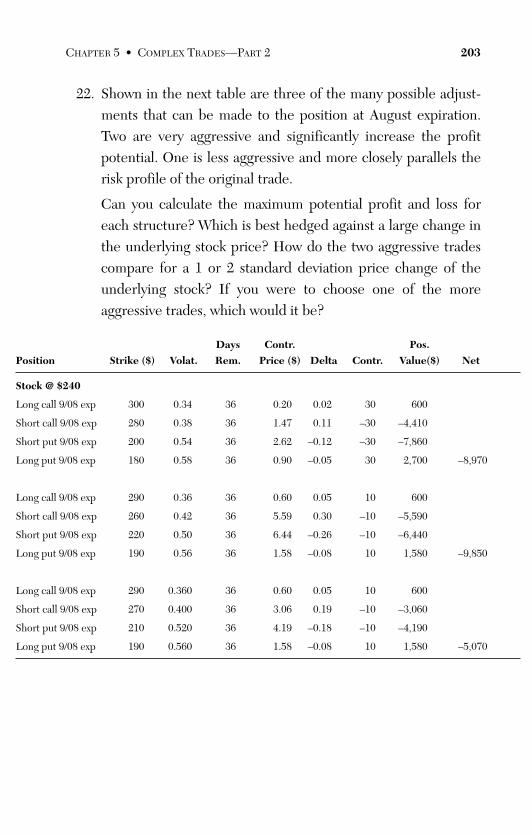
ptg
22. Shown in the next table are three of the many possible adjust-ments that can be made to the position at August expiration.Two are very aggressive and significantly increase the profitpotential. One is less aggressive and more closely parallels therisk profile of the original trade.
Can you calculate the maximum potential profit and loss foreach structure? Which is best hedged against a large change inthe underlying stock price? How do the two aggressive tradescompare for a 1 or 2 standard deviation price change of theunderlying stock? If you were to choose one of the moreaggressive trades, which would it be?
CHAPTER 5 • COMPLEX TRADES—PART 2 203
Days Contr. Pos.Position Strike ($) Volat. Rem. Price ($) Delta Contr. Value($) Net
Stock @ $240
Long call 9/08 exp 300 0.34 36 0.20 0.02 30 600
Short call 9/08 exp 280 0.38 36 1.47 0.11 –30 –4,410
Short put 9/08 exp 200 0.54 36 2.62 –0.12 –30 –7,860
Long put 9/08 exp 180 0.58 36 0.90 –0.05 30 2,700 –8,970
Long call 9/08 exp 290 0.36 36 0.60 0.05 10 600
Short call 9/08 exp 260 0.42 36 5.59 0.30 –10 –5,590
Short put 9/08 exp 220 0.50 36 6.44 –0.26 –10 –6,440
Long put 9/08 exp 190 0.56 36 1.58 –0.08 10 1,580 –9,850
Long call 9/08 exp 290 0.360 36 0.60 0.05 10 600
Short call 9/08 exp 270 0.400 36 3.06 0.19 –10 –3,060
Short put 9/08 exp 210 0.520 36 4.19 –0.18 –10 –4,190
Long put 9/08 exp 190 0.560 36 1.58 –0.08 10 1,580 –5,070
From the Library of Melissa Wong
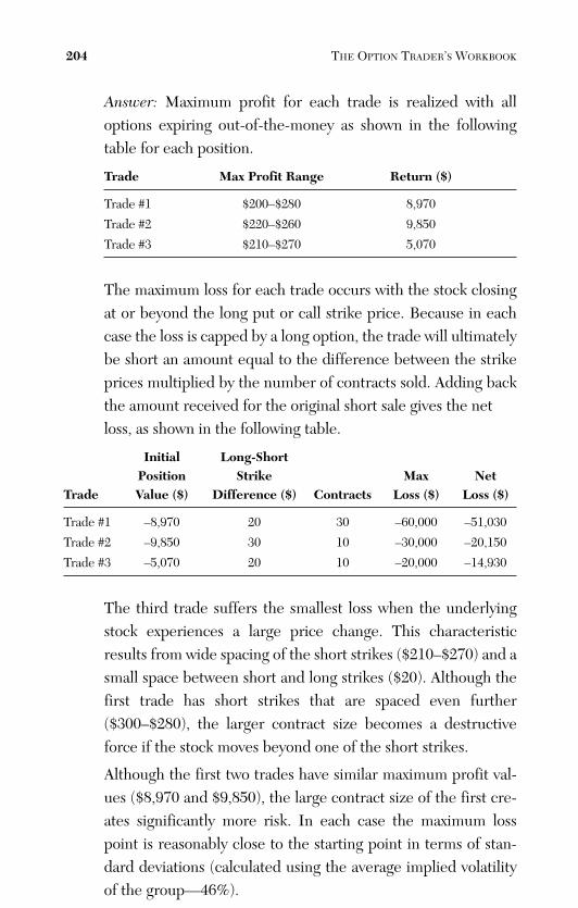
ptg
Answer: Maximum profit for each trade is realized with alloptions expiring out-of-the-money as shown in the followingtable for each position.
Trade Max Profit Range Return ($)
Trade #1 $200–$280 8,970
Trade #2 $220–$260 9,850
Trade #3 $210–$270 5,070
The maximum loss for each trade occurs with the stock closingat or beyond the long put or call strike price. Because in eachcase the loss is capped by a long option, the trade will ultimatelybe short an amount equal to the difference between the strikeprices multiplied by the number of contracts sold. Adding backthe amount received for the original short sale gives the net loss, as shown in the following table.
Initial Long-ShortPosition Strike Max Net
Trade Value ($) Difference ($) Contracts Loss ($) Loss ($)
Trade #1 –8,970 20 30 –60,000 –51,030
Trade #2 –9,850 30 10 –30,000 –20,150
Trade #3 –5,070 20 10 –20,000 –14,930
The third trade suffers the smallest loss when the underlyingstock experiences a large price change. This characteristicresults from wide spacing of the short strikes ($210–$270) and asmall space between short and long strikes ($20). Although thefirst trade has short strikes that are spaced even further($300–$280), the larger contract size becomes a destructiveforce if the stock moves beyond one of the short strikes.
Although the first two trades have similar maximum profit val-ues ($8,970 and $9,850), the large contract size of the first cre-ates significantly more risk. In each case the maximum losspoint is reasonably close to the starting point in terms of stan-dard deviations (calculated using the average implied volatilityof the group—46%).
204 THE OPTION TRADER’S WORKBOOK
From the Library of Melissa Wong
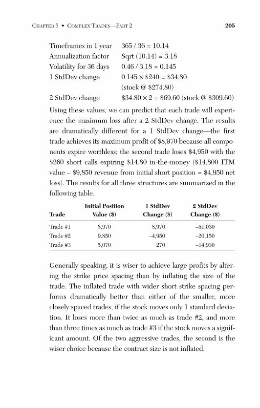
ptg
Timeframes in 1 year 365 / 36 = 10.14Annualization factor Sqrt (10.14) = 3.18Volatility for 36 days 0.46 / 3.18 = 0.1451 StdDev change 0.145 × $240 = $34.80
(stock @ $274.80)2 StdDev change $34.80 × 2 = $69.60 (stock @ $309.60)
Using these values, we can predict that each trade will experi-ence the maximum loss after a 2 StdDev change. The resultsare dramatically different for a 1 StdDev change—the firsttrade achieves its maximum profit of $8,970 because all compo-nents expire worthless; the second trade loses $4,950 with the$260 short calls expiring $14.80 in-the-money ($14,800 ITMvalue – $9,850 revenue from initial short position = $4,950 netloss). The results for all three structures are summarized in thefollowing table.
Initial Position 1 StdDev 2 StdDev Trade Value ($) Change ($) Change ($)
Trade #1 8,970 8,970 –51,030
Trade #2 9,850 –4,950 –20,150
Trade #3 5,070 270 –14,930
Generally speaking, it is wiser to achieve large profits by alter-ing the strike price spacing than by inflating the size of thetrade. The inflated trade with wider short strike spacing per-forms dramatically better than either of the smaller, moreclosely spaced trades, if the stock moves only 1 standard devia-tion. It loses more than twice as much as trade #2, and morethan three times as much as trade #3 if the stock moves a signif-icant amount. Of the two aggressive trades, the second is thewiser choice because the contract size is not inflated.
CHAPTER 5 • COMPLEX TRADES—PART 2 205
From the Library of Melissa Wong
ptg
Volatility Index (Problems #23–#24)
The Chicago Board Options Exchange Volatility Index (VIX) is aclosely followed, widely studied metric of overall market volatility. Itis not calculated using the Black-Scholes pricing model; instead, ituses a formula that averages the weighted prices of out-of-the-moneyputs and calls for S&P 500 stocks. The contribution of a single optionto the index value is proportional to its price and inversely propor-tional to the strike. Calculations generally span the two nearest-termexpiration months; however, in the final 8 days before expiration, thewindow is rolled forward to the second and third contract months tominimize pricing anomalies that occur just before expiration.
Building on historical information contained in its databases, theCBOE has made available calculated values of the index dating backto 1986. These data have become an important research tool for thoseattempting to understand the behavior of equity markets. They arealso valuable to investors seeking a hedge against large market draw-downs. Trading activities are supported by investment productsoffered by the CBOE; on March 26, 2004, VIX futures began tradingon the CBOE futures exchange, and VIX options were launched inFebruary 2006. The CBOE website is an excellent primary source ofinformation about the VIX and other volatility indexes.
Unlike equity options, VIX options are European-style expira-tion—that is, they can be exercised only on the final day. Additionally,instead of expiring on the same day as equity options, VIX optionsexpire on the Wednesday that is 30 days prior to the third Friday ofthe month immediately following the expiration month. Furthermore,expiration occurs at the open, and the contracts are valued usingopening quotations of S&P 500 index options.
23. Figure 5.1 displays an implied volatility skew for VIX calloptions with 70 days remaining before expiration and the indexat 25. Strike prices are displayed on the x-axis and impliedvolatility on the y-axis.
206 THE OPTION TRADER’S WORKBOOK
From the Library of Melissa Wong
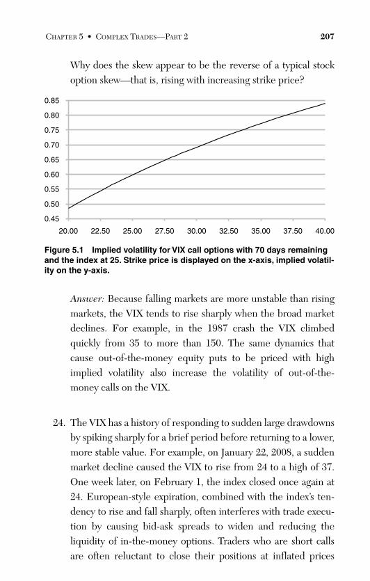
ptg
Why does the skew appear to be the reverse of a typical stockoption skew—that is, rising with increasing strike price?
CHAPTER 5 • COMPLEX TRADES—PART 2 207
0.45
0.50
0.55
0.60
0.65
0.70
0.75
0.80
0.85
20.00 22.50 25.00 27.50 30.00 32.50 35.00 37.50 40.00
Figure 5.1 Implied volatility for VIX call options with 70 days remainingand the index at 25. Strike price is displayed on the x-axis, implied volatil-ity on the y-axis.
Answer: Because falling markets are more unstable than risingmarkets, the VIX tends to rise sharply when the broad marketdeclines. For example, in the 1987 crash the VIX climbedquickly from 35 to more than 150. The same dynamics thatcause out-of-the-money equity puts to be priced with highimplied volatility also increase the volatility of out-of-the-money calls on the VIX.
24. The VIX has a history of responding to sudden large drawdownsby spiking sharply for a brief period before returning to a lower,more stable value. For example, on January 22, 2008, a suddenmarket decline caused the VIX to rise from 24 to a high of 37.One week later, on February 1, the index closed once again at24. European-style expiration, combined with the index’s ten-dency to rise and fall sharply, often interferes with trade execu-tion by causing bid-ask spreads to widen and reducing theliquidity of in-the-money options. Traders who are short callsare often reluctant to close their positions at inflated prices
From the Library of Melissa Wong
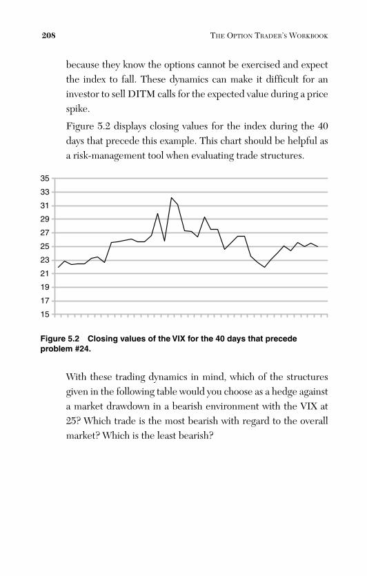
ptg
because they know the options cannot be exercised and expectthe index to fall. These dynamics can make it difficult for aninvestor to sell DITM calls for the expected value during a pricespike.
Figure 5.2 displays closing values for the index during the 40days that precede this example. This chart should be helpful asa risk-management tool when evaluating trade structures.
208 THE OPTION TRADER’S WORKBOOK
15
17
19
21
23
25
27
29
31
33
35
Figure 5.2 Closing values of the VIX for the 40 days that precedeproblem #24.
With these trading dynamics in mind, which of the structuresgiven in the following table would you choose as a hedge againsta market drawdown in a bearish environment with the VIX at25? Which trade is the most bearish with regard to the overallmarket? Which is the least bearish?
From the Library of Melissa Wong
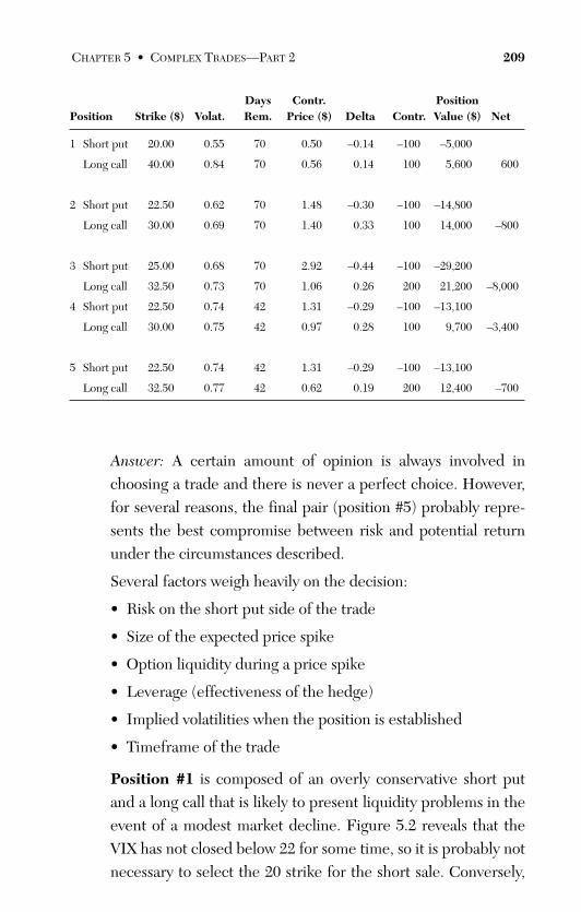
ptg
Days Contr. PositionPosition Strike ($) Volat. Rem. Price ($) Delta Contr. Value ($) Net
1 Short put 20.00 0.55 70 0.50 –0.14 –100 –5,000
Long call 40.00 0.84 70 0.56 0.14 100 5,600 600
2 Short put 22.50 0.62 70 1.48 –0.30 –100 –14,800
Long call 30.00 0.69 70 1.40 0.33 100 14,000 –800
3 Short put 25.00 0.68 70 2.92 –0.44 –100 –29,200
Long call 32.50 0.73 70 1.06 0.26 200 21,200 –8,000
4 Short put 22.50 0.74 42 1.31 –0.29 –100 –13,100
Long call 30.00 0.75 42 0.97 0.28 100 9,700 –3,400
5 Short put 22.50 0.74 42 1.31 –0.29 –100 –13,100
Long call 32.50 0.77 42 0.62 0.19 200 12,400 –700
Answer: A certain amount of opinion is always involved inchoosing a trade and there is never a perfect choice. However,for several reasons, the final pair (position #5) probably repre-sents the best compromise between risk and potential returnunder the circumstances described.
Several factors weigh heavily on the decision:
• Risk on the short put side of the trade
• Size of the expected price spike
• Option liquidity during a price spike
• Leverage (effectiveness of the hedge)
• Implied volatilities when the position is established
• Timeframe of the trade
Position #1 is composed of an overly conservative short putand a long call that is likely to present liquidity problems in theevent of a modest market decline. Figure 5.2 reveals that theVIX has not closed below 22 for some time, so it is probably notnecessary to select the 20 strike for the short sale. Conversely,
CHAPTER 5 • COMPLEX TRADES—PART 2 209
From the Library of Melissa Wong
ptg
the 40 strike is 25% above the highest recent peak of the index.This trade, therefore, anticipates a market decline that is signif-icantly larger than the drawdown that caused the peak seen inthe figure. With expiration 70 days away, it might prove difficultto close the long side of the trade for a fair price if the VIX spikeis generally viewed as temporary. Compounding this problem isthe cost of the long 40 strike calls (84% implied volatility). Exe-cuting this trade involves selling 55% implied volatility and pur-chasing 84%—the skew is biased against the trade.
Position #2 is an improvement over position #1. It is less con-servative on the short side but very likely too conservative onthe long side. Since we know that the index has recently risenabove 30, it would be unreasonable to forego the leverage of aslightly higher strike. Position #2 suffers from the same time-frame issues as position #1.
Position #3 has a tremendous advantage over the previous twopositions because it is structured with a 2:1 contract size lever-age advantage—each short put at the 25 strike pays for 2 calls atthe 32.5 strike. This trade is extremely bearish with regard tothe overall market because it assumes that the VIX will remainabove its current level and is initially net short $8,000. Unlikethe other trades, this structure is designed to profit from timedecay even if the market does not experience a significantdrawdown. Unfortunately, a 2.5-point decline to recent indexlevels would generate a $17,000 (213%) loss. A 5-point declinewould cost $42,000. As in the first two structures, time untilexpiration might cause a liquidity problem in a brief drawdown.This position, being the most bearish, is likely to be used as aprofit engine in a long-term weak market rather than a portfoliohedge.
Position #4 has several advantages, including a conservativeshort strike and near-dated expiration. As in position #2, thelong strike is below the recent peak and probably would not be
210 THE OPTION TRADER’S WORKBOOK
From the Library of Melissa Wong
ptg
selected if the goal is to hedge against a significant marketdecline. This trade is the least bearish because it generates a$3,400 profit even if the market rallies slightly and the VIX falls2.5 points.
Position #5 is the best portfolio hedge candidate because itcombines the leverage characteristics of trade #3 with the moreconservative short strike and timeframe of position #4. A mod-est spike to recent levels would generate a significant profit,and the near-dated options would likely be more liquid thanthose of the first three positions. Like position #4, this trade canwithstand a modest rally that lowers the VIX by 10%. Overall, itis likely the best choice for hedging in a bear market.
Dividend Arbitrage (Problem #25)
25. An impending dividend payment can often be exploited to gen-erate a profit. However, because option prices always compre-hend the effect of a dividend payment the moment it isannounced, structuring the proper trade can be complex.
Assume that a $95 stock will pay a $0.50-per-share dividendwhen the market opens tomorrow. Which of the options in thefollowing table can be used as part of a trade structure that willgenerate profit after the dividend is paid? How would thattrade be structured?
Days ContractPosition Strike ($) Stock ($) Remaining Price ($) Theta
1 Call 90 95 14 6.40 –0.10
2 Put 100 95 14 6.00 –0.10
CHAPTER 5 • COMPLEX TRADES—PART 2 211
From the Library of Melissa Wong
ptg
Answer: The $100 put (option #2) can be used as part of a tradeconsisting of long stock and long puts. Success depends on theput being underpriced—a signal that the market does not antic-ipate a drop in the stock equal to the value of the dividend pay-ment. The stock purchase completes the arbitrage by hedgingagainst a large price increase. We can assume that the put isunderpriced because it has 10¢ per day of time decay with 14days remaining before expiration. Multiplying these two num-bers yields a minimum of $1.40 of time value that must beadded to the amount that the option is in-the-money. We can,therefore, state that the option should trade for approximately$6.40, and that the market anticipates an underlying stock priceincrease.
If we were to purchase 10 puts along with 1,000 shares of stockand the underlying price fell to $94.50, the put price would riseto $6.80 ($5.50 ITM value + $1.30 remaining time). Our tradewould, therefore, generate a loss of $0.50 on the stock side anda gain of $0.80 on the option side. Since the stock-side loss isoffset by a $0.50 per share dividend, the trade would net $800.
Conversely, if the stock price increased to $95.50, the put pricecould be expected to fall $0.20 to $5.80 ($4.50 ITM value +$1.30 remaining time). The combined trade would experience anet gain of $0.30. Adding the $0.50 per share dividend onceagain yields a profit of $800.
Although these gains are small, they are characteristic of arbi-trage trades that are designed to exploit very subtle pricing inef-ficiencies. In most cases such trades generate returns that aretoo small to be exploited by public customers who pay commis-sions and full bid-ask spreads.
The call version of this trade would involve purchasing under-priced calls and shorting stock. In this scenario, an underlyingprice decrease would result in a gain from the short stock thatmore than offsets the loss on the originally underpriced calls as
212 THE OPTION TRADER’S WORKBOOK
From the Library of Melissa Wong
ptg
their value resets. A price increase would result in a dispropor-tionate rise in the call price that would more than offset theshort stock loss. However, the $90 call price displayed in thetable appears not to be discounted, and it is likely that gains orlosses on the call side would be offset by the short stock. Thecall trade also suffers because it does not include long stockand, therefore, does not receive a dividend payment.
Finally, arbitrage trades of this sort can also be structured toexploit overpriced options. The put version would consist ofshort puts/short stock, and the call version would be composedof short calls/long stock. Most price distortions that arise from adividend payment involve either underpriced puts or over-priced calls. These anomalies make sense because the marketoften anticipates that the stock will fall less than the amount ofthe dividend. Many investors mistakenly believe that in-the-money call prices are guaranteed to fall and in-the-money putprices guaranteed to rise by an amount equal to the dividend.They typically point to a delta of 1.0 and assume that the optionwill move with the stock. As a result, they often sell calls or buyputs expecting an automatic profit. These scenarios represent ariskless arbitrage that cannot occur because nobody would evertake the other side of the trade. Surprisingly, calls can gainvalue when the stock falls if they are initially underpriced, andputs can lose value if they are overpriced. It is always better toidentify a mispriced option and construct a fully hedged tradethan to guess the direction.
CHAPTER 5 • COMPLEX TRADES—PART 2 213
From the Library of Melissa Wong
ptg
Summary
This chapter was designed to explore the trade managementdynamics of a representative group of multipart structures. Thesetrades are important because they provide very high levels of flexibilityand risk management. As we have seen, it is possible to construct con-servative trades that are hedged against large underlying stock pricechanges but also deliver stable returns. Complex multipart trades arethe domain of the conservative investor seeking stability. By combiningpricing mathematics with market statistics, knowledgeable investorscan take advantage of a myriad of choices regarding strike price andexpiration date for each component of a trade. Some investors believethat such trades have too many “moving parts.” This view is contra-dicted by the large number of successful option traders who continu-ally generate predictable income streams using these strategies.
214 THE OPTION TRADER’S WORKBOOK
From the Library of Melissa Wong
ptg
Glossary
American-Style Option An option that can be exercised at anytime prior to expiration.
Arbitrage Simultaneous purchase and sale of the same or equiva-lent security on the same or different markets in order to profit fromprice discrepancies. Many authors mistakenly define arbitrage asbuying in one market and selling in another to take advantage of aprice disparity. However, more often than not, arbitrage tradingoccurs across equivalent financial instruments in the same market.For example, the simultaneous purchase of stock and an equivalentnumber of mispriced put options can often be used to structure anarbitrage prior to a dividend payment. This trade, properly executed,is riskless. Merger arbitrage involving the exchange of stock betweencompanies and arbitrages that are related to put-call parity violationsare also common variations. In all cases the trade must be riskless tobe considered an arbitrage.
At-the-Money An option whose exercise (strike) price is equal tothe current trading price of the underlying security. The term issometimes used to refer to the option whose strike price is closest tothe current trading price of the underlying.
215
From the Library of Melissa Wong
ptg
Backspread A structure in which more options are purchasedthan sold but at a less favorable strike. A call backspread is estab-lished by selling calls at a lower strike and purchasing more at ahigher strike.
Bear Spread A trade consisting of long and short contracts havingdifferent strike prices and/or expiration dates that increase in valuewhen the price of the underlying security declines.
Bull Spread A trade consisting of long and short contracts havingdifferent strike prices and/or expiration dates that increases in valuewhen the price of the underlying security rises.
Butterfly The sale (purchase) of two options with the same strikeprice along with the purchase (sale) of one option at a lower strikeand one option with a higher strike. All options must be the sametype (call or put) and have the same expiration date. Exercise pricesmust be symmetrically spaced. For example, the structure 10 long$100 calls/20 short $110 calls/10 long $120 calls is a long butterfly.
Calendar Spread A position consisting of long and short compo-nents that spans different expirations—a time spread.
Condor The sale (purchase) of two options with different exerciseprices along with the purchase (sale) of one option at a lower strikeand one with a higher strike. All options must be the same type (callor put) and have the same expiration date. Exercise prices must besymmetrically spaced. For example, the structure 10 long $100calls/10 short $110 calls/10 short $120 calls/10 long $130 calls is along condor. Such trades are designed to profit from time decay; theoutside long positions, also known as “wings,” are hedges againstlarge price changes. Short condors in which the inside strikes arepurchased are designed to generate profit when the underlying secu-rity moves a substantial amount. In this case the wings are used tooffset time decay costs.
216 THE OPTION TRADER’S WORKBOOK
From the Library of Melissa Wong
ptg
Covered Call A structure consisting of long stock and an equiva-lent number of short calls. Covered call positions can also be estab-lished using long calls instead of stock. In the pure option case, thelong option must have more favorable terms—that is, the same orlater expiration and the same or lower strike.
Covered Put A structure consisting of short stock and an equiva-lent number of long puts. Covered put positions can also be estab-lished using long puts instead of short stock. In the pure optioncase, the long option must have more favorable terms—that is, thesame or later expiration and the same or higher strike.
Delta The sensitivity of an option price to a change in the price ofthe underlying security. For equity options, delta is measured as theeffect of a $1 increase in the underlying. Call options have positivedeltas and put options have negative deltas.
Delta-Neutral A position in which the sum of all deltas—longand short—is approximately zero.
Diagonal Spread A structure consisting of long and short optionshaving different strike prices and expiration dates. Both sides of thetrade must be the same type (call or put).
European-Style Option An option that can be exercised only atexpiration.
Gamma The sensitivity of an option delta to a change in the priceof the underlying security. For equity options gamma is measured aschange in delta that accompanies a $1 increase in the underlying.Gamma can also be used to refer to an overall position or a portfo-lio. Hedge funds often track portfolio gamma because it is an impor-tant measure of risk. Generally speaking, it is dangerous to be shortlarge amounts of gamma. The value is always positive regardless ofthe type of option because delta increases for both puts and callswhen the underlying price rises—put delta becomes less negativeand call delta becomes more positive.
GLOSSARY 217
From the Library of Melissa Wong
ptg
Implied Volatility The volatility derived from a known optionprice using associated parameters—underlying security price, timeleft before expiration, and risk-free interest rate.
In-the-Money A term used to describe an option with intrinsicvalue. A call option is described as in-the-money when the underly-ing security trades below the strike price. The reverse is true for aput option, which is in-the-money when the underlying trades above the strike.
Intrinsic Value The value of an option with all time premiumremoved—that is, the value if it were to expire immediately. Forcalls in which the strike is below the stock price, this value is equal tothe stock price minus the strike price. For puts in which the strike isabove the stock price, this value is equal to the strike price minus thestock price.
Out-of-the-Money A term used to describe an option with nointrinsic value. A call option is described as out-of-the-money whenthe underlying security trades above the strike price. The reverse istrue for a put option, which is out-of-the-money when the underly-ing trades below the strike.
Ratio Strategy Any strategy built around unequal numbers oflong and short securities.
Ratio Vertical Spread A trade consisting of long and short options(calls or puts) in which a greater number are sold at the more distantstrike and all contracts have the same expiration date. In most casesthe initial position is structured so as to be delta-neutral.
Rho The change in value of an option price that results from a 1%increase in the risk-free interest rate. Rho is larger for long-term orin-the-money options.
218 THE OPTION TRADER’S WORKBOOK
From the Library of Melissa Wong
ptg
Straddle A position consisting of equal numbers of long (short)calls and long (short) puts having the same expiration date and strike price.
Strangle A position consisting of equal numbers of long (short)calls and long (short) puts having the same expiration date and dif-ferent strike prices.
Synthetic Stock A structure composed of a long (short) call and ashort (long) put in which both options have the same expiration dateand strike price. The long call/short put combination is equivalent tolong stock; short call/long put is equivalent to short stock.
Term Structure Measures the effect of time on implied volatility.Term structure can be visualized in a plot of implied volatility for at-the-money options versus expiration month. Its behavior tends tocompress the shape of the smile curve as the maturity dateincreases. (See Volatility Skew.)
Theta The amount of value that an option loses for each day of timethat passes. Theta increases as expiration approaches, causing optionvalues to fall more quickly near expiration. The Black-Scholes pricingformulas can be used to derive an accurate value for theta at any pointin the expiration cycle if the underlying price, strike price, impliedvolatility or option price, and risk-free rate of return are known.
Time Value The price of an option minus its intrinsic value. Thevalue of an out-of-the-money option is equal to its time value.
Vega The change in value of an option price that results from a1% increase in implied volatility.
Vertical Spread A structure composed of long and short optionsof the same type (calls or puts) expiring on the same date with differ-ent strike prices.
GLOSSARY 219
From the Library of Melissa Wong
ptg
Volatility Skew Describes the phenomenon in which impliedvolatility varies with strike price in the same month. The best-knownskew is the “volatility smile,” which causes out-of-the-money puts tobe more expensive than option pricing theory would normally pre-dict. The volatility smile became much more pronounced after thestock market crash of October 1987. Since then, implied volatilityprofiles for equity and index options have taken on a distinctly nega-tive skew—that is, implied volatility tends to rise as the strike pricedecreases. Additionally, because put-call parity dictates that the rela-tionship between strike price and implied volatility is the same forboth types of contracts, in-the-money calls are also more expensive.The complete smile takes the form of an asymmetric curve that risesslightly above the trading price of the underlying security—that is,out-of-the-money calls also exhibit implied volatility increases. In afamily of volatility smile curves containing one curve per month, thesteepness of each successive curve becomes less pronounced.
220 THE OPTION TRADER’S WORKBOOK
From the Library of Melissa Wong
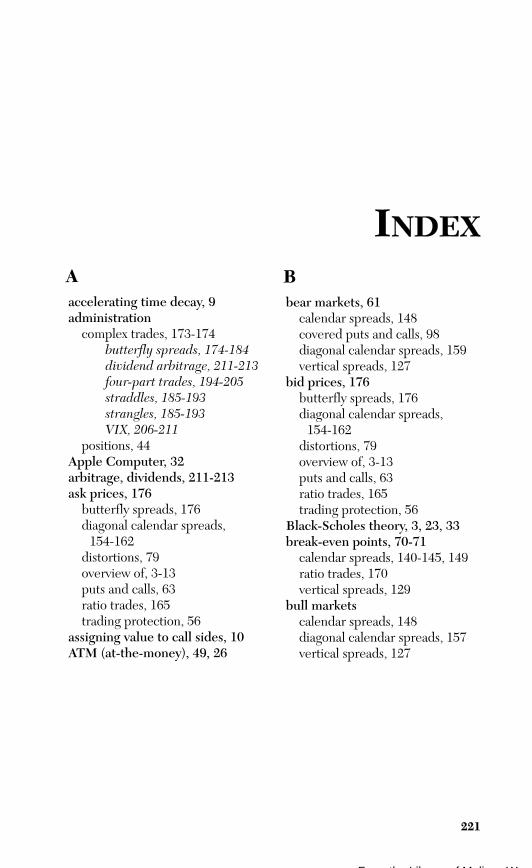
ptg
INDEX
Aaccelerating time decay, 9administration
complex trades, 173-174butterfly spreads, 174-184dividend arbitrage, 211-213four-part trades, 194-205straddles, 185-193strangles, 185-193VIX, 206-211
positions, 44Apple Computer, 32arbitrage, dividends, 211-213ask prices, 176
butterfly spreads, 176diagonal calendar spreads,
154-162distortions, 79overview of, 3-13puts and calls, 63ratio trades, 165trading protection, 56
assigning value to call sides, 10ATM (at-the-money), 49, 26
221
Bbear markets, 61
calendar spreads, 148covered puts and calls, 98diagonal calendar spreads, 159vertical spreads, 127
bid prices, 176butterfly spreads, 176diagonal calendar spreads,
154-162distortions, 79overview of, 3-13puts and calls, 63ratio trades, 165trading protection, 56
Black-Scholes theory, 3, 23, 33break-even points, 70-71
calendar spreads, 140-145, 149ratio trades, 170vertical spreads, 129
bull marketscalendar spreads, 148diagonal calendar spreads, 157vertical spreads, 127
From the Library of Melissa Wong
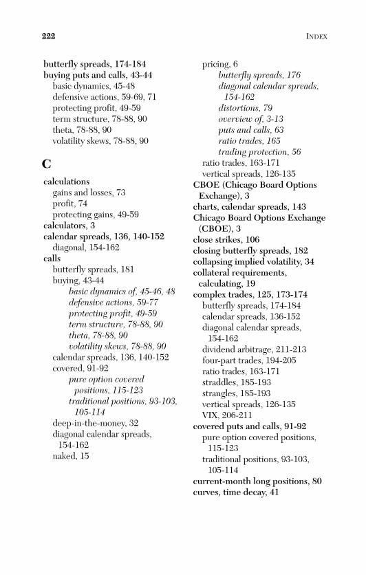
ptg
222 INDEX
butterfly spreads, 174-184buying puts and calls, 43-44
basic dynamics, 45-48defensive actions, 59-69, 71protecting profit, 49-59term structure, 78-88, 90theta, 78-88, 90volatility skews, 78-88, 90
Ccalculations
gains and losses, 73profit, 74protecting gains, 49-59
calculators, 3calendar spreads, 136, 140-152
diagonal, 154-162calls
butterfly spreads, 181buying, 43-44
basic dynamics of, 45-46, 48defensive actions, 59-77protecting profit, 49-59term structure, 78-88, 90theta, 78-88, 90volatility skews, 78-88, 90
calendar spreads, 136, 140-152covered, 91-92
pure option coveredpositions, 115-123
traditional positions, 93-103,105-114
deep-in-the-money, 32diagonal calendar spreads,
154-162naked, 15
pricing, 6butterfly spreads, 176diagonal calendar spreads,
154-162distortions, 79overview of, 3-13puts and calls, 63ratio trades, 165trading protection, 56
ratio trades, 163-171vertical spreads, 126-135
CBOE (Chicago Board OptionsExchange), 3
charts, calendar spreads, 143Chicago Board Options Exchange
(CBOE), 3close strikes, 106closing butterfly spreads, 182collapsing implied volatility, 34collateral requirements,
calculating, 19complex trades, 125, 173-174
butterfly spreads, 174-184calendar spreads, 136-152diagonal calendar spreads,
154-162dividend arbitrage, 211-213four-part trades, 194-205ratio trades, 163-171straddles, 185-193strangles, 185-193vertical spreads, 126-135VIX, 206-211
covered puts and calls, 91-92pure option covered positions,
115-123traditional positions, 93-103,
105-114current-month long positions, 80curves, time decay, 41
From the Library of Melissa Wong
ptg
INDEX 223
Ddaily volatility, adjusting, 25decay (time)
butterfly spreads, 177curves, 41overview of, 9pricing, 6-7
deep-in-the-money, 26, 32deep-out-of-the-money, 26defensive actions, buying puts
and calls, 59-69, 71-77deltas, 12
at-the-money calls, 36butterfly spreads, 177calendar spreads, 148covered puts and calls, 109diagonal calendar spreads, 157expiration, 38neutral point migration, 18ratio trades, 169values, 15
distortions, pricing, 79DITM options, 96dividend arbitrage, 211-213
E–Fearnings releases, 29equations, Black-Scholes, 3equity, options, 27European options, 24expiration, 13
butterfly spreads, 181calendar spreads, 137covered puts and calls, 96, 100deltas, 38diagonal calendar spreads,
154-162long-dated, 118monthly, 115
option positions, 45pricing, 5trading price protection, 56
far strikes, 106far-dated options, 121flattening of volatility skews, 83four-part trades, 194-205
G–Hgains
butterfly spreads, 176calculating, 73calendar spreads, 147four-part trades, 198ratio trades, 163strike prices, 64vertical spreads, 133
gamma, 12effect of volatility, 14
hedges, 54complex trades, 173-174
butterfly spreads, 174-184dividend arbitrage, 211-213four-part trades, 194-205straddles, 185-193strangles, 185-193VIX, 206-211
stocks, 15
I–Jimplied volatility, 27. See also
volatilityin-the-money, 26indexes
options, 27Volatility Index (VIX), 24,
206-211
From the Library of Melissa Wong
ptg
224 INDEX
K–Lleverage
definition of, 46performance, 48
liquidationdefensive actions, 61positions, 51profit, protecting, 51
lognormal distribution, 10long butterfly trades, 178. See
also butterfly spreadslong DITM puts, 131long position yields, 69long-dated expirations, 44, 118losses, 64
calculating, 73calendar spreads, 137, 147covered puts and calls, 108diagonal calendar spreads, 160four-part trades, 197profit, 69puts and calls, buying, 59-77ratio trades, 163vertical spreads, 128
Mmanagement
complex trades, 173-174butterfly spreads, 174-184dividend arbitrage, 211-213four-part trades, 194-205straddles, 185-193strangles, 185-193VIX, 206-211
positions, 44monthly expirations, 115multiple expirations, diagonal
calendar spreads, 154-162
N–Onaked calls, 15near-dated options, 14, 121neutral point of straddles, 16normal distribution, 26NORMSDIST function, 58, 66
offsetting time decay, 7one-month calendar spreads,
value of, 75options
butterfly spreads, 182covered puts and calls, 91
pure option coveredpositions, 115-123
traditional positions, 93-103,105-114
DITM, 96far-dated, 121near-dated, 121positions, expiration, 45trading, 125. See also trading
OTM (out-of-the-money), 26, 49options, 14pricing, 6
Pparity violations, 23performance, leverage, 48positions
covered, 91-92pure option covered,
115-123traditional, 93-103, 105-114
liquidating, 51management, 44options, expiration, 45
predrawdown prices, 85
From the Library of Melissa Wong
ptg
INDEX 225
pricingbutterfly spreads, 176diagonal calendar spreads,
154-162distortions, 79overview of, 3-13puts and calls, 63ratio trades, 165trading protection, 56
profiles, risk-adjusted, 67profit
calculating, 74calendar spreads, 149covered puts and calls, 100diagonal calendar spreads,
158-160four-part trades, 204losses, 69protecting, 49-59vertical spreads, 131
purchasing. See buying putsand calls
pure option covered positions,115-123
putsbuying, 43-44
basic dynamics, 45-48defensive actions, 59-77protecting profit, 49-59term structure, 78-88, 90theta, 78-88, 90volatility skews, 78-88, 90
calendar spreads, 136-152calls. See callscovered, 91-92
pure option coveredpositions, 115-123
traditional positions, 93-103,105-114
diagonal calendar spreads, 154-162
pricing, 5put-call parity violations, 23ratio trades, 163-171vertical spreads, 126-135
Q–Rrallies, stocks, 49ratio trades, 163-171rho, 31risk
complex trades, 173-174butterfly spreads, 174-184dividend arbitrage, 211-213four-part trades, 194-205straddles, 185-193strangles, 185-193VIX, 206-211
covered puts and calls, 122risk-adjusted
maximum returns, 65profiles, 67
risk-free interest, raising valueof, 8
Sselling
basic dynamics, 45-48calls, 53covered puts and calls, 112defensive actions, 59-69, 71protecting profit, 49-59stocks. See stocksterm structure, 78-88, 90theta, 78-88, 90volatility skews, 78-88, 9
short side expiration, 69short-dated expirations, 44shorting delta-equivalent number
of shares, 62
From the Library of Melissa Wong
ptg
226 INDEX
spreadsbutterfly, 174-184calendar, 136-144, 146-152diagonal calendar, 154-162vertical, 126-135
standard deviation decline, 167StdDev, 108steep volatility smiles, 132stocks
covered puts and callspure option covered
positions, 115-123traditional positions, 93-103,
105-114hedges, 15pricing, 6
butterfly spreads, 176diagonal calendar spreads,
154-162distortions, 79overview of, 3-13puts and calls, 63ratio trades, 165trading protection, 56
rallies, 49straddles, 16, 185-193strangles, 185-193strategies, buying puts and
calls, 43strike prices. See also pricing
covered puts and calls, 94diagonal calendar spreads,
154-162structure of volatility, 32synthetic short sales, 130synthetic stock positions, 36
Tterm structure, 78- 85, 87-90theta. See also time decay
puts and calls, buying, 78-88, 90time decay
butterfly spreads, 177curves, 41overview of, 9pricing, 6-7
timeframes, calendar spreads, 152tools, pricing, 3-13trading
buying. See buying puts and callscomplex trades, 125, 173-174
butterfly spreads, 174-184calendar spreads, 136,
140-152diagonal calendar spreads,
154-162dividend arbitrage, 211-213four-part trades, 194-205ratio trades, 163-171straddles, 185-193strangles, 185-193vertical spreads, 126-135volatility index (VIX),
206-211covered puts and calls, 91pricing. See also selling
overview of, 5-15, 19-28protection, 56
From the Library of Melissa Wong
ptg
INDEX 227
U–Vunanticipated negative news,
effect on stock prices, 85
valuesdeltas, 15one-month calendar spreads, 75
vega, 30butterfly spreads, 178
vertical spreads, 126-135violations, parity, 23VIX (Volatility Index), 24,
206-211volatility
effect of gamma, 14calculating, 25calendar spreads, 140covered puts and calls, 113increasing, 7pricing, 6profit, protecting, 57skews, 78-88, 90smiles, 31structure of, 32zero, approaching, 17
Volatility Index (VIX), 24, 206-211
W–Zx-axis, 6
y-axis, 6yields, long positions, 69
From the Library of Melissa Wong
ptg
JEFF AUGEN, currently a private investor and writer, has spent more than a decade building a unique intellectual property portfolio of databases, algorithms, and associated software for technical analysis of derivatives prices. His work, which includes more than a million lines of computer code, is particularly focused on the identification of subtle anomalies and price distortions.
As a cofounding executive of IBM’s Life SciencesComputing business, he defined a growth strategy that resulted in $1.2 billion of new revenue and managed a large portfolio of venture capital investments. From 2002-2005, he was President/CEO of TurboWorx, a software company founded by the chairman of the Department of Computer Science at Yale University. He is the author of two previous books: The Volatility Edge in Options Trading (FT Press 2008) and Bioinformatics in the Post-Genomic Era (Addison-Wesley 2005).
Cover design and art by Chuti PrasertsithCover photo by Gregor Schuster/ Photographer’s Choice /Getty Images
ABOUT THE AUTHOR
Press
www.ftpress.com | An imprint of Pearson
From the Library of Melissa Wong