Embed Size (px)
Citation preview
From polar night to midnight sun: Diel vertical migration, metabolismand biogeochemical role of zooplankton in a high Arctic fjord(Kongsfjorden, Svalbard)
G. Darnis,1* L. Hobbs,2 M. Geoffroy,3,4 J. C. Grenvald,5 P. E. Renaud,1,5 J. Berge,4,5 F. Cottier,2,4
S. Kristiansen,4 M. Daase,4 J. E. Søreide,5 A. Wold,6 N. Morata,1 T. Gabrielsen5
1Akvaplan-niva. Fram Centre for Climate and the Environment, Tromsø, Norway2Scottish Association for Marine Science, Oban, United Kingdom3Universit�e Laval, Pavillon Alexandre-Vachon, Qu�ebec, Qu�ebec, Canada4Faculty of Biosciences, Fisheries and Economics, UiT The Arctic University of Norway, Tromsø, Norway5University Centre in Svalbard, Longyearbyen, Norway6Norwegian Polar Institute, Tromsø, Norway
Abstract
Zooplankton vertical migration enhances the efficiency of the ocean biological pump by translocating car-
bon (C) and nitrogen (N) below the mixed layer through respiration and excretion at depth. We measured C
and N active transport due to diel vertical migration (DVM) in a Svalbard fjord at 798N. Multifrequency analysis
of backscatter data from an Acoustic Zooplankton Fish Profiler moored from January to September 2014, com-
bined with plankton net data, showed that Thysanoessa spp. euphausiids made up>90% of the diel migrant
biomass. Classical synchronous DVM occurred before and after the phytoplankton bloom, leading to a mis-
match with intensive primary production during the midnight sun. Zooplankton DVM resulted in C respira-
tion of 0.9 g m22 and ammonium excretion of 0.18 g N m22 below 82 m depth between February and April,
and 0.2 g C m22 and 0.04 g N m22 from 11 August to 9 September, representing>25% and>33% of sinking
flux of particulate organic carbon and nitrogen, respectively. Such contribution of DVM active transport to the
biological pump in this high-Arctic location is consistent with previous measurements in several equatorial to
subarctic oceanic systems of the World Ocean. Climate warming is expected to result in tighter coupling
between DVM and bloom periods, stronger stratification of the Barents Sea, and northward advection of boreal
euphausiids. This may increase the role of DVM in the functioning of the biological pump on the Atlantic side
of the Arctic Ocean, particularly where euphausiids are or will be prevalent in the zooplankton community.
The World Ocean plays a critical role in the mitigation of
the planetary greenhouse effect due to CO2 by absorbing
about one third of the anthropogenic emissions of carbon to
the atmosphere (Marinov and Sarmiento 2004). The oceanic
uptake of CO2 is regulated by physical and chemical process-
es, referred to as the “solubility pump,” and a complex set of
biological processes known as the “biological pump”
(Ducklow et al. 2001). The mechanics of the latter involve
the fixation of inorganic carbon by phytoplankton
photosynthesis in the photic layer and subsequent vertical
translocation of pelagic new primary production, either by
sinking (passive or sinking flux) or transport (active flux), to
depth below a pycnocline (Longhurst and Harrison 1988;
Steinberg et al. 2000; Steinberg et al. 2002).
In the temperate and tropical ocean, extensive diel vertical
migration (DVM) of zooplankton and micronekton has been
shown to play a significant role in the vertical flux of particu-
late and dissolved organic matter (Longhurst et al. 1990; Stein-
berg et al. 2002; Takahashi et al. 2009). Active transport can
represent up to 70% and 82% of the sinking fluxes of particu-
late organic carbon (POC), and nitrogen (PON), respectively
(Dam et al. 1995). Typically, herbivorous zooplankton feed in
the epipelagic layer at night and migrate to depth before
dawn to avoid predation by visual predators (Brierley 2014).
There they release carbon and nitrogen during egestion, and
as CO2 and NH14 through respiration and excretion (Bronk
and Steinberg 2008; Steinberg et al. 2008).
*Correspondence: [email protected]
Additional Supporting Information may be found in the online versionof this article.
This is an open access article under the terms of the Creative Commons
Attribution License, which permits use, distribution and reproduction inany medium, provided the original work is properly cited.
1
LIMNOLOGYand
OCEANOGRAPHYLimnol. Oceanogr. 00, 2017, 00–00
VC 2017 The Authors Limnology and Oceanography published by Wiley Periodicals, Inc.on behalf of Association for the Sciences of Limnology and Oceanography
doi: 10.1002/lno.10519
In Arctic ecosystems, the high seasonality in light climate,
shifting between the “polar night” (when the sun remains
below the horizon) and “midnight sun” (when the sun does
not set for extended periods) seasons makes zooplankton
DVM responses more complex than at lower latitudes (Ring-
elberg 2010; Last et al. 2016). The rapid changes in day-
night cycle and other environmental factors affect timing,
synchrony, and vertical range of migration (Fischer and Vis-
beck 1993; Berge et al. 2014), which in turn influence the
transport potential over the year. In such a variable light
environment, snapshot sampling during scientific cruises
limits the assessment of the consequences of zooplankton
DVM. However, studies using multi-month time-series of
acoustic data from moored instruments have shed light on
the seasonal patterns of DVM. Acoustic Doppler current pro-
filers (ADCPs) have recorded periods where zooplankton
behavior resembles classical DVM, when the relative rate of
change in irradiance is sufficient to trigger synchronous
movements of zooplankton in winter-spring and autumn.
The data have also suggested unsynchronized (individual)
vertical movements under the continuous illumination of
the Arctic summer when algal food is usually plentiful in the
surface layer (Cottier et al. 2006; Berge et al. 2009; Wallace
et al. 2010). Plankton-net data, sometimes combined with
acoustic data, have shown that euphausiids, hyperiid amphi-
pods, large Calanus and Metridia copepods, chaetognaths,
and ctenophores are the main diel migrants in Arctic waters,
their relative importance fluctuating with seasons and loca-
tions (Fischer and Visbeck 1993; Fortier et al. 2001; Daase
et al. 2008; Berge et al. 2014).
One study based on a 10-month analysis of zooplankton
in the southeastern Beaufort Sea revealed the importance of
seasonal vertical migration (SVM) for carbon budgets in Arc-
tic systems (Darnis and Fortier 2012). Carbon export below
200 m depth, mediated by large seasonal migrants such as
the Arctic copepods Calanus hyperboreus and Calanus glacialis
that overwinter at depth, was found to be of the same mag-
nitude as the annual sinking POC flux measured by sedi-
ment traps. The impacts of both the well-known DVM
taking place during the lighted season (Cottier et al. 2006;
Wallace et al. 2010) and the recently discovered DVM during
polar night (Berge et al. 2009; Wallace et al. 2010), however,
have not been estimated. It is likely that ongoing DVM by
some components of the community during winter will add
to the proportion of vertical flux during this season
accounted for by SVM. The consequences of DVM for the
biological pump around the time of maximum new produc-
tion are difficult to predict, however. This information is
needed if we are to forecast the response of the Arctic marine
ecosystem to the rapid warming of its waters and potential
alteration of timing of ecological processes and the faunal
assemblages present (Ardyna et al. 2014).
Here, we document the effect of synchronous DVM
on the export to depth of carbon and nitrogen, using a
7-month time series of acoustic data collected with a moored
acoustic zooplankton fish profiler (AZFP) in combination
with plankton-net sampling in a high-Arctic Svalbard fjord,
Kongsfjorden. In particular, we measure remineralization of
carbon through respiration and excretion of ammonium at
depth and assess the importance of the active transport rela-
tive to other fluxes.
Methods
Environmental setting of the study area
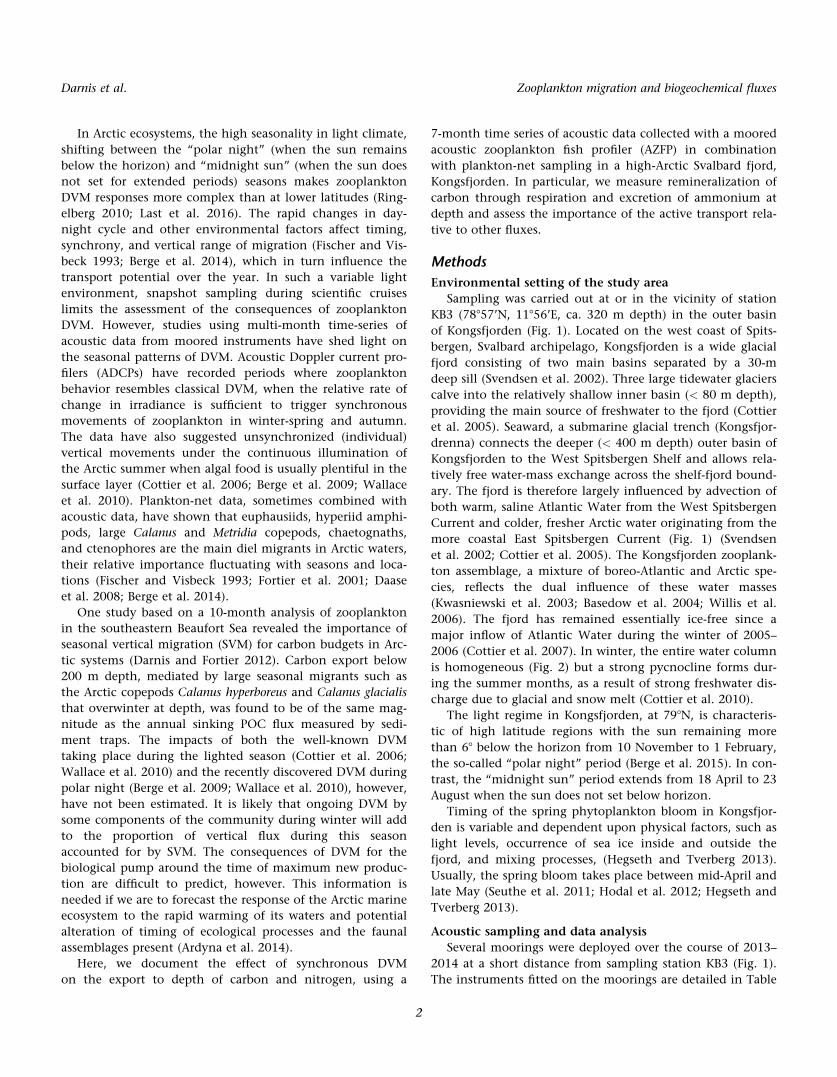
Sampling was carried out at or in the vicinity of station
KB3 (78857’N, 11856’E, ca. 320 m depth) in the outer basin
of Kongsfjorden (Fig. 1). Located on the west coast of Spits-
bergen, Svalbard archipelago, Kongsfjorden is a wide glacial
fjord consisting of two main basins separated by a 30-m
deep sill (Svendsen et al. 2002). Three large tidewater glaciers
calve into the relatively shallow inner basin (< 80 m depth),
providing the main source of freshwater to the fjord (Cottier
et al. 2005). Seaward, a submarine glacial trench (Kongsfjor-
drenna) connects the deeper (< 400 m depth) outer basin of
Kongsfjorden to the West Spitsbergen Shelf and allows rela-
tively free water-mass exchange across the shelf-fjord bound-
ary. The fjord is therefore largely influenced by advection of
both warm, saline Atlantic Water from the West Spitsbergen
Current and colder, fresher Arctic water originating from the
more coastal East Spitsbergen Current (Fig. 1) (Svendsen
et al. 2002; Cottier et al. 2005). The Kongsfjorden zooplank-
ton assemblage, a mixture of boreo-Atlantic and Arctic spe-
cies, reflects the dual influence of these water masses
(Kwasniewski et al. 2003; Basedow et al. 2004; Willis et al.
2006). The fjord has remained essentially ice-free since a
major inflow of Atlantic Water during the winter of 2005–
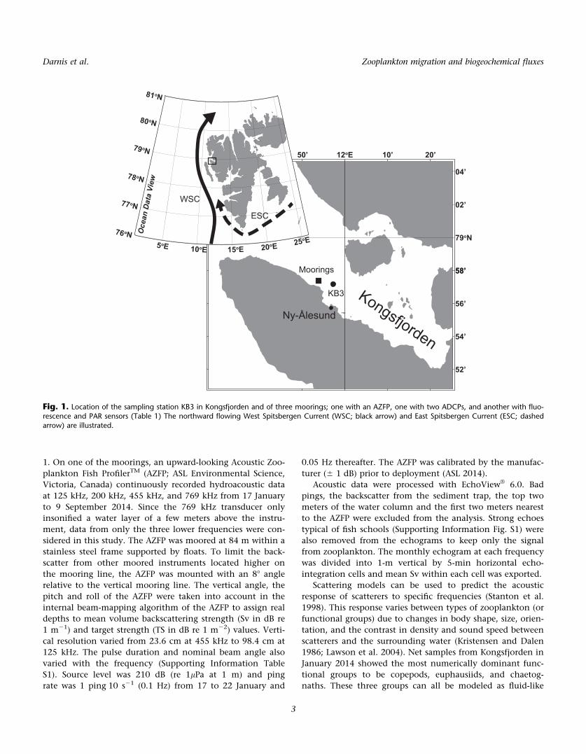
2006 (Cottier et al. 2007). In winter, the entire water column
is homogeneous (Fig. 2) but a strong pycnocline forms dur-
ing the summer months, as a result of strong freshwater dis-
charge due to glacial and snow melt (Cottier et al. 2010).
The light regime in Kongsfjorden, at 798N, is characteris-
tic of high latitude regions with the sun remaining more
than 68 below the horizon from 10 November to 1 February,
the so-called “polar night” period (Berge et al. 2015). In con-
trast, the “midnight sun” period extends from 18 April to 23
August when the sun does not set below horizon.
Timing of the spring phytoplankton bloom in Kongsfjor-
den is variable and dependent upon physical factors, such as
light levels, occurrence of sea ice inside and outside the
fjord, and mixing processes, (Hegseth and Tverberg 2013).
Usually, the spring bloom takes place between mid-April and
late May (Seuthe et al. 2011; Hodal et al. 2012; Hegseth and
Tverberg 2013).
Acoustic sampling and data analysis
Several moorings were deployed over the course of 2013–
2014 at a short distance from sampling station KB3 (Fig. 1).
The instruments fitted on the moorings are detailed in Table
Darnis et al. Zooplankton migration and biogeochemical fluxes
2
1. On one of the moorings, an upward-looking Acoustic Zoo-
plankton Fish ProfilerTM (AZFP; ASL Environmental Science,
Victoria, Canada) continuously recorded hydroacoustic data
at 125 kHz, 200 kHz, 455 kHz, and 769 kHz from 17 January
to 9 September 2014. Since the 769 kHz transducer only
insonified a water layer of a few meters above the instru-
ment, data from only the three lower frequencies were con-
sidered in this study. The AZFP was moored at 84 m within a
stainless steel frame supported by floats. To limit the back-
scatter from other moored instruments located higher on
the mooring line, the AZFP was mounted with an 88 angle
relative to the vertical mooring line. The vertical angle, the
pitch and roll of the AZFP were taken into account in the
internal beam-mapping algorithm of the AZFP to assign real
depths to mean volume backscattering strength (Sv in dB re
1 m21) and target strength (TS in dB re 1 m22) values. Verti-
cal resolution varied from 23.6 cm at 455 kHz to 98.4 cm at
125 kHz. The pulse duration and nominal beam angle also
varied with the frequency (Supporting Information Table
S1). Source level was 210 dB (re 1lPa at 1 m) and ping
rate was 1 ping�10 s21 (0.1 Hz) from 17 to 22 January and
0.05 Hz thereafter. The AZFP was calibrated by the manufac-
turer (6 1 dB) prior to deployment (ASL 2014).
Acoustic data were processed with EchoViewVR 6.0. Bad
pings, the backscatter from the sediment trap, the top two
meters of the water column and the first two meters nearest
to the AZFP were excluded from the analysis. Strong echoes
typical of fish schools (Supporting Information Fig. S1) were
also removed from the echograms to keep only the signal
from zooplankton. The monthly echogram at each frequency
was divided into 1-m vertical by 5-min horizontal echo-
integration cells and mean Sv within each cell was exported.
Scattering models can be used to predict the acoustic
response of scatterers to specific frequencies (Stanton et al.
1998). This response varies between types of zooplankton (or
functional groups) due to changes in body shape, size, orien-
tation, and the contrast in density and sound speed between
scatterers and the surrounding water (Kristensen and Dalen
1986; Lawson et al. 2004). Net samples from Kongsfjorden in
January 2014 showed the most numerically dominant func-
tional groups to be copepods, euphausiids, and chaetog-
naths. These three groups can all be modeled as fluid-like
Ny-Ålesund
KB3
76oN
77oN
78oN
79oN
80oN
81oN
5oE 10oE 15oE 20oE 25oE
Oce
an D
ata
View
Moorings
Kongsfjorden
12oE
79oN
56’
58’
02’
54’
52’
04’
50’
58’
10’ 20’
WSC
ESC
Fig. 1. Location of the sampling station KB3 in Kongsfjorden and of three moorings; one with an AZFP, one with two ADCPs, and another with fluo-rescence and PAR sensors (Table 1) The northward flowing West Spitsbergen Current (WSC; black arrow) and East Spitsbergen Current (ESC; dashedarrow) are illustrated.
Darnis et al. Zooplankton migration and biogeochemical fluxes
3
weak scatterers (Stanton and Chu 2000) using the Distorted
Wave Born Approximation approach (Stanton et al. 1998).
Scattering models were fitted for each functional group using
a range of sizes (Supporting Information Table S2) and
specific orientation angles for copepods (Benfield et al.
2000), euphausiids (Chu et al. 1993) and chaetognaths
(Fredrika Norrbin; unpubl. Video Plankton Recorder data
from Kongsfjorden), at the three frequencies of the AZFP.
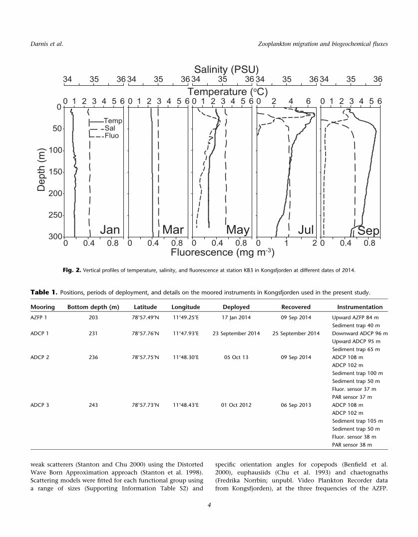
Table 1. Positions, periods of deployment, and details on the moored instruments in Kongsfjorden used in the present study.
Mooring Bottom depth (m) Latitude Longitude Deployed Recovered Instrumentation
AZFP 1 203 78857.49’N 11849.25’E 17 Jan 2014 09 Sep 2014 Upward AZFP 84 m
Sediment trap 40 m
ADCP 1 231 78857.76’N 11847.93’E 23 September 2014 25 September 2014 Downward ADCP 96 m
Upward ADCP 95 m
Sediment trap 65 m
ADCP 2 236 78857.75’N 11848.30’E 05 Oct 13 09 Sep 2014 ADCP 108 m
ADCP 102 m
Sediment trap 100 m
Sediment trap 50 m
Fluor. sensor 37 m
PAR sensor 37 m
ADCP 3 243 78857.73’N 11848.43’E 01 Oct 2012 06 Sep 2013 ADCP 108 m
ADCP 102 m
Sediment trap 105 m
Sediment trap 50 m
Fluor. sensor 38 m
PAR sensor 38 m
Dep
th (m
)
0
50
100
150
200
250
300
0 2 4 6Temperature (oC)
34 35 36Salinity (PSU)
34 35 36 34 35 36
0 0.4 0.8 0 0.4 0.8 0 0.4 0.8Jan Mar May
Fluorescence (mg m-3)
TempSalFluo
1 3 5 0 2 4 61 3 5 0 2 4 61 3 5
34 35 36 34 35 36
0 1 0 0.4 0.8Jul Sep
0 2 4 6 0 2 4 61 3 5
2
Fig. 2. Vertical profiles of temperature, salinity, and fluorescence at station KB3 in Kongsfjorden at different dates of 2014.
Darnis et al. Zooplankton migration and biogeochemical fluxes
4
These models demonstrated that euphausiids have a
frequency response of Sv125kHz> Sv200kHz< Sv455kHz; cope-
pods of Sv125kHz< Sv200kHz< Sv455kHz; and chaetognaths
Sv125kHz< Sv200kHz> Sv455kHz. Using these differences in the
frequency responses, each echo-integration cell was parti-
tioned into one of the three functional groups, which was
assumed to be dominant within that given cell.
Mean TS for each functional group was then estimated
based on the randomly oriented fluid bent cylinder model
(Stanton et al. 1994). The average dry weight W of individu-
al euphausiids and copepods was estimated from measure-
ments of individuals made on a microbalance whereas the
W of chaetognaths was estimated using a length-dry weight
relationship established for Parasagitta elegans (Welch et al.
1996) (Supporting Information Table S2). Mean dry biomass
(mg m23) within each echo-integration cell associated with
euphausiids (Eq. 1), copepods (Eq. 2), or chaetognaths (Eq.
3) was calculated following Parker-Stetter et al. (2009):
Biomasseuphausiids5sv125kHz
rbseuphausiids
!�Weuphausiids (1)
Biomasscopepods5sv455kHz
rbscopepodss
!�Wcopepods (2)
Biomasschaetognaths5sv200kHz
rbschaetognaths
!�Wchaetognaths (3)
Where sv is the linear volume backscattering strength (m2
m23), rbs is the expected backscattering cross-section of an
element of the zooplankton group (m22), and W is the aver-
age dry weight (mg). The biomass of each zooplankton
group was integrated in the top 2–40 m (above the trap) and
2–82 m layers and averaged for each month during the day
and the night hours. Day was defined as the time-interval of
minimum backscatter in the targeted water layer around
local midday measured on the echogram at 125 kHz of the
AZFP (Supporting Information Fig. S2), whereas night was
the period of higher backscatter during the remainder of the
24-h cycle. Dry biomass was converted to carbon content
using the C : W factor of 0.5189, 0.5366, and 0.3844 for
euphausiids (i.e., Thysanoessa inermis), large copepods, and
chaetognaths (i.e., P. elegans), respectively (Ikeda and Skjol-
dal 1989).
To gain insight into the zooplankton DVM patterns
beyond the period sampled with the AZFP (until 9 Septem-
ber), additional acoustic data were obtained during a short-
term mooring deployment close to the autumn equinox (23–
25 September). The mooring was equipped with two 307-
kHz RDI ADCPs, one upward-looking at 95 m, the other
downward-looking at 96 m. In addition, a Parflux 21-cup
sediment trap was positioned at 65 m to intercept sinking
particles and zooplankton swimmers (Table 1). The ADCPs
measured the mean echo strength from ensembles of 60
pings at a rate of 1 ping s21 in 22 depth layers (bins of 4 m).
The raw echo intensity data were converted to a measure of
absolute volume backscatter (Sv, in dB) (Berge et al. 2014).
The ADCPs would detect zooplankton of the size of medium
to large Calanus copepodite stages (> 5 mm of prosome
length) and larger.
A Seapoint fluorometer and photosynthetic active radia-
tion (PAR) sensor, both mounted at 37 m depth on an adja-
cent mooring, provided raw fluorescence and PAR data in
the vicinity of station KB3 from 5 October 2013 to 9 Septem-
ber 2014.
Ship-based sampling and taxonomic analysis
Net sampling for macro- and meso-zooplankton was car-
ried out at station KB3 using R/V Helmer Hanssen from 16 to
20 January and 23 to 27 September 2014. Additional meso-
zooplankton samples were taken between 12 and 14 May,
using the workboat Teisten, and on 23 July using R/V Lance.
Macrozooplankton was sampled as close as possible to local
midday and midnight by trawling obliquely from 30 m
depth to the surface at two knots for approximately 5–10
min with a Methot-Isaac-Kidd (MIK) ring net (3.15 m2 aper-
ture, 13-m long net with 1500 lm mesh size, and a 500 lm
mesh in the last meter), fitted with a 10-L cod end and
equipped with a Hydrobios flowmeter at the center of the
ring. Upon retrieval, the zooplankton samples were subdi-
vided and 2/3 to 3/4 of the cod end was fixed in a borax-
buffered seawater solution of 4% formaldehyde for taxonom-
ic identification. Nine and four MIK net deployments were
done in January and September, respectively.
Mesozooplankton was sampled around midday and mid-
night, using a Hydro-Bios multiple plankton sampler Midi-
MultiNet (0.25 m2 aperture, 5 nets of 200-lm mesh) hauled
vertically at 0.5 m min21. The sample depths were 320–
200 m, 200–100 m, 100–50 m, 50–20 m, and 20–0 m depth.
In May, successive deployments of a KC Denmark WP2 net
(0.25 m2 aperture, 200-lm mesh) with a closing system were
done instead of the MultiNet sampling, and the deepest stra-
tum sampled reached 300 m depth. No replicate sampling of
each depth stratum was performed. Upon collection, the
content of the cod ends was preserved in seawater solution
of 4% hexamethylen-buffered formaldehyde for taxonomic
identification. Four MultiNet deployments were performed
in January, three in May, one in July, and four in September.
CTD (Seabird SBE 911) casts through the water column were
carried out immediately before or after net deployments to
collect profiles of temperature, salinity, and fluorescence.
In January, May, and September, additional MIK and Mul-
tiNet/WP2 casts were carried out at station KB3 to catch live
zooplankton for respiration, ammonium excretion, and bio-
mass measurements. The sampling using a WP2 or WP3
(1 m2 aperture, 1000-lm mesh) net was performed on the
Svalbard shelf from 18 to 28 May for mesozooplankton respi-
ration measurement onboard Helmer Hanssen. Each net of
the samplers was fitted with a rigid cod end with filtration
Darnis et al. Zooplankton migration and biogeochemical fluxes
5
apertures at the top of the cylinder to keep the animals in
sufficient water until collection. Upon retrieval, each sample
was diluted in cold filtered (0.2–0.7 lm GF/F) seawater and
any large jellyfish were removed. Other macrozooplankton
such as amphipods, euphausiids, and Clione limacina were
also removed from the samples collected with the MultiNet/
WP2 to avoid predation and stress on the mesozooplankton
size class. The live samples were kept in the dark in a
temperature-controlled room set at close to in situ tempera-
ture (1–48C) until further treatment.
In the laboratory, known aliquots (up to 1/8) were taken
from the MIK formalin-preserved macrozooplankton samples
and all non-copepod organisms were counted and identified
to species level under a stereomicroscope before measuring
their total body length. Samples from the MultiNet casts
were size-fractionated on a 1000-lm sieve and re-suspended
in distilled water. Successive known aliquots were taken
from the 200-lm to 1000-lm fraction with a 5-mL large tip
(> 5 mm diameter) automatic pipette until 300 organisms
were counted and identified to developmental stage and spe-
cies, or to the lowest possible taxonomic level, under a ste-
reomicroscope. The>1000-lm fraction was analyzed in its
entirety. Prosome length of the Calanus copepodites was
measured in both size-fractions.
Zooplankton biomass, respiration, and ammonium
excretion
Intact and active individuals of dominant macrozooplank-
ton taxa, essentially Thysanoessa spp., Themisto abyssorum,
and Themisto libellula, were rapidly sorted from the MIK live
samples. A known subsample of each of the live samples col-
lected with the MultiNet/WP2 was poured into a funnel fit-
ted with a 1000-lm sieve inside and a gate valve to obtain
two mesozooplankton size classes for incubation.
The>1000-lm fraction was retained in the top part of the
device in a sufficient volume of water while the 200–1000
lm small zooplankton was gently evacuated through the
sieve through successive washes with cold oxygenated, fil-
tered seawater. A sufficient number of macrozooplankton
animals (1–10 depending on size and volume of incubation
bottle) and each mesozooplankton size class were gently
introduced in separate airtight glass bottles (110–280 mL
capacity), which were thereafter filled with cold oxygenated
filtered seawater and capped. Control bottles without zoo-
plankton were made in triplicates for each experimental set-
up. Oxygen concentration was measured by optode
respirometry with a 4-channel respirometer (Oxy-4 Mini,
PreSens Precision Sensing GmbH, Regensburg, Germany)
every 0.5–2 h for 8–12 h. Respiration rates were calculated
by determining the slope of the decrease of oxygen over
time and subtracting the mean value for the controls. Oxy-
gen consumption rates were transformed to respiratory car-
bon using a respiratory quotient of 0.75 in January,
assuming a winter metabolism mainly by lipid reserves
(Ingvarsd�ottir et al. 1999), and 0.97 from May onward with a
metabolism primarily based on proteins (Gnaiger 1983).
Zooplankton ammonium (NH14 ) excretion rate was esti-
mated from the same incubations used for respiration and
calculated as the difference in NH14 concentration between
incubation bottles and animal-free control bottles at the end
of the experiment divided by the duration of incubation to
obtain an hourly rate. In January, ammonium concentration
was measured onboard immediately after collection while, in
September, the water samples were preserved in acid-cleaned
125-mL polycarbonate bottles and immediately frozen. Dur-
ing the January and September fieldwork, triplicate samples
of water were taken before the incubation for ammonium
measurement. At termination of incubation, triplicate sam-
ples were retrieved from the incubation water. The ammoni-
um samples were filtered through acid-washed Sartorius
polycarbonate syringe filter holders equipped with pre-
burned Whatman GF/C glass microfibre filters (6 h at
4508C). The filter holders were rinsed with deionized Milli-Q
water before use. NH4-N concentration was analyzed spectro-
fluorimetrically using a 5-cm cell following Sol�orzano (1969).
Right after the experiments organisms were carefully blot-
ted on absorbent material and preserved in cryovials at
2208C. In the laboratory, the frozen samples were trans-
ferred to pre-weighed plastic cups, dried in an oven at 608C
for 48 h and then weighed on a microbalance (6 1 lg). Car-
bon content (C) of each macro- and meso-zooplankton tax-
on was calculated from dry mass (W) measurements, using
the specific C-W relationship in Ikeda and Skjoldal (1989).
Active respiratory carbon and excretory nitrogen
transport
To study the seasonal variation in zooplankton DVM pat-
terns (spatial extent and strength in terms of biomass
involved), and resulting active fluxes of carbon and nitrogen,
the daily migrant biomass MB (mg C m22) of euphausiids,
copepods, and chaetognaths was calculated. Monthly aver-
ages of migrant biomass integrated from surface to depth (z)
over the 7-month time series were determined from Eq. 4:
MBz5
ðz
night biomass2day biomass (4)
Transport out of the top 2–40 m and 2–82 m depth strata was
considered. The lower limit of the layer (z) was set at 40 m
depth for comparison of active transport with sinking flux
measured with a sediment trap at that depth whereas z at 82 m
corresponds to the maximum depth sampled with the AZFP.
The downward active transport at depth z was then calcu-
lated using Eq. 5:
AFz5MB3RE3T (5)
where AF is the active transport of carbon (mg C m22 d21)
or nitrogen (mg N m22 d21) by migrant zooplankton, RE is
Darnis et al. Zooplankton migration and biogeochemical fluxes
6
the specific hourly respiratory carbon loss (mg C mg C21
h21) or ammonium excretion (mg N mg C21 h21), and T (h)
is the time spent at depth during a 24-h cycle. T was mea-
sured from the AZFP echogram at 125 kHz.
To calculate daily rates of community respiration, excre-
tion and active transport due to DVM averaged over each
month of the time-series, hourly specific metabolic rates of
the different taxa and size classes had to be interpolated by
using the three snapshot measurements of hourly rates of
January, May, and late September to cover the whole study
period. For mesozooplankton, we assumed that the size class-
>1000 lm largely dominated by large copepods was primari-
ly responsible for the backscatter recorded by the AZFP, and
applied their specific hourly metabolic rates in the calcula-
tions. Chaetognath metabolic rates were not measured due
to the difficulty of collecting undamaged individuals for
incubations. Thus, we used a specific respiration of
0.40 6 1.06 lg C mg C21 h21 and excretion of 0.15 6 0.12 lg
N mg C21 h21, measured by Ikeda and Skjoldal (1989) on P.
elegans, the dominant chaetognath in Kongsfjorden.
Sinking flux of POC and PON
To compare our estimates of active transport of carbon
and nitrogen below the 40 m and 82 m depths with sinking
fluxes of POC and PON, we analyzed samples from sequen-
tial automated sediment traps (McLane PARFLUX Mark78H;
0.66 m2 collecting area; 21-cups turntable) deployed on
moorings in Kongsfjorden (Table 1). A sediment trap at 40 m
depth on the same mooring as the AZFP intercepted sinking
particles from 21 January to 3 April 2014 at a sampling fre-
quency of 3.5 d per cup. A large volume of terrigenous mat-
ter clogged a sediment trap at 100 m depth soon after
deployment in October 2013, preventing from using the sed-
iment samples to quantify sinking fluxes in the annual cycle
2013–2014. Therefore, we used the 2012–2013 time series of
sediment samples to quantify POC and PON sinking at
100 m depth, assuming a low interannual variability in sink-
ing fluxes outside of the bloom period.
Before deployment, the sample cups were filled with sea-
water filtered through Whatman GF/F 0.7 lm glass fiber fil-
ters, adjusted to 35 PSU with NaCl, and poisoned with
formalin (2% v/v, sodium borate buffered). After recovery,
zooplankton were removed from the samples using a dissect-
ing microscope. Samples were then subdivided using a
Motoda splitting box and filtered in triplicates through pre-
weighed GF/F filters (25 mm diameter, 0.7 lm pore, pre-
combusted for 4 h at 4508C). Filters were dried for 12 h at
608C, weighed for dry weight and exposed to concentrated
HCl fumes for 12 h to remove inorganic carbon. They were
folded in tin cups that were then combusted in a
EuroEA3022 elemental analyzer for measurement of POC
and PON.
Results
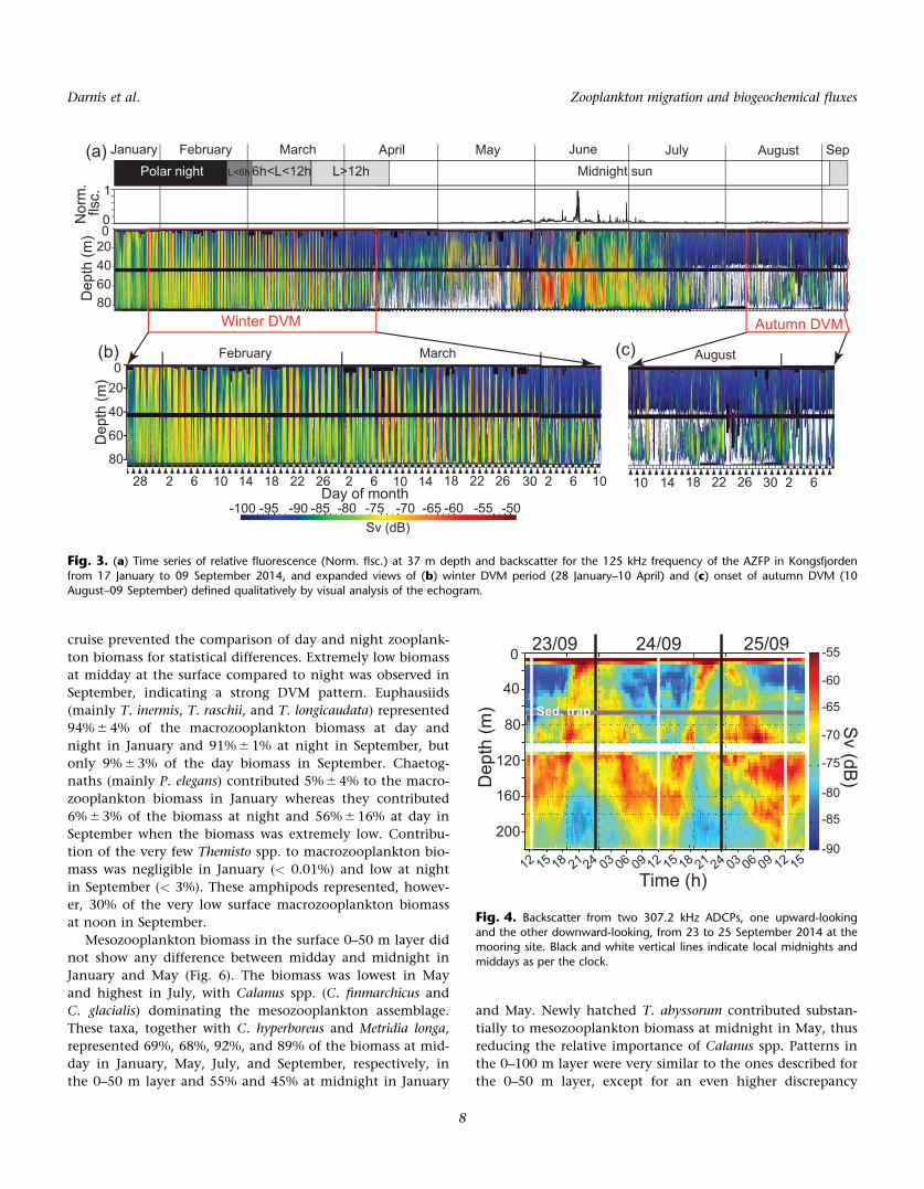
Synchronous DVM
The continuous echogram of the AZFP at 125 kHz allows
for the tracking of vertical distribution of scatterers over the
7-month period from the polar night to the end of summer.
DVM behavior was identified qualitatively as periods of time
where a strong scattering layer characterized by a strong
band of green/red was seen to oscillate at a daily frequency
over a depth range greater than 30 m (Fig. 3a). A clearly visi-
ble synchronous DVM extending below 40 m started on 28
January (Fig. 3b). From then on the depth range of the DVM
signal increased, reaching 82 m on 31 January. This winter
DVM persisted until 10 April (a few days before the onset of
midnight sun), after which sporadic synchronous vertical
movements did not usually occur in phase with the 24-h
light cycle. Synchronous DVM resumed on 11 August, first
with weak sporadic migrations (not every day), that reached
a regular 24-h period in early September (Fig. 3c). Thus, clas-
sical DVM behavior occurred outside of the main season of
primary production, between late May and late June in 2014
as shown by the fluorescence at 37 m depth (Fig. 3a). Strong
echoes during the midnight sun in June and early July in
the 2–82 m layer, indicative of strong zooplankton biomass
but without evidence of classical DVM, coincided with this
period of high biological production in the surface layer.
The echogram of the backscatter recorded by the ADCPs
over 3 d in late September, 2 weeks after the end of the
AZFP sampling, shows a strong DVM signal (Fig. 4). At mid-
night, the bulk of the backscatter was concentrated in the
upper 20 m, whereas it was located between 120 m and
160 m at midday.
Time spent at depth during a 24-h cycle
Time spent by scatterers below 40 m and below 82 m dur-
ing a daily cycle showed a very similar strong linear increase
from the start of DVM in late January to its end in April (Fig.
5). From early March onward, the small difference between
times spent below 40 m and below 82 m indicated that the
downward/upward migrations were swift from surface to
below the two depth limits. From January to early March,
zooplankton spent most of a diel cycle above 40 m or 80 m
depth, with time at depth<12 h. Conversely, at the end of
the late winter DVM period when there was more than 12 h
of light per day, zooplankton were distributed below 82 m
most of the day (> 20 h). The same situation can be seen in
late August and early September at the onset of the autumn
synchronous DVM season.
Composition of the migratory community from plankton
net data
Macrozooplankton biomass in the surface 0–30 m layer
estimated from the plankton net hauls tended to be slightly
lower at midday than at midnight in January (Fig. 6). How-
ever, the low number of net deployments during each short
Darnis et al. Zooplankton migration and biogeochemical fluxes
7
cruise prevented the comparison of day and night zooplank-
ton biomass for statistical differences. Extremely low biomass
at midday at the surface compared to night was observed in
September, indicating a strong DVM pattern. Euphausiids
(mainly T. inermis, T. raschii, and T. longicaudata) represented
94% 6 4% of the macrozooplankton biomass at day and
night in January and 91% 6 1% at night in September, but
only 9% 6 3% of the day biomass in September. Chaetog-
naths (mainly P. elegans) contributed 5% 6 4% to the macro-
zooplankton biomass in January whereas they contributed
6% 6 3% of the biomass at night and 56% 6 16% at day in
September when the biomass was extremely low. Contribu-
tion of the very few Themisto spp. to macrozooplankton bio-
mass was negligible in January (< 0.01%) and low at night
in September (< 3%). These amphipods represented, howev-
er, 30% of the very low surface macrozooplankton biomass
at noon in September.
Mesozooplankton biomass in the surface 0–50 m layer did
not show any difference between midday and midnight in
January and May (Fig. 6). The biomass was lowest in May
and highest in July, with Calanus spp. (C. finmarchicus and
C. glacialis) dominating the mesozooplankton assemblage.
These taxa, together with C. hyperboreus and Metridia longa,
represented 69%, 68%, 92%, and 89% of the biomass at mid-
day in January, May, July, and September, respectively, in
the 0–50 m layer and 55% and 45% at midnight in January
and May. Newly hatched T. abyssorum contributed substan-
tially to mesozooplankton biomass at midnight in May, thus
reducing the relative importance of Calanus spp. Patterns in
the 0–100 m layer were very similar to the ones described for
the 0–50 m layer, except for an even higher discrepancy
Sed. trap
-55
-60
-65
-70
-75
-80
-85
-90
Sv (dB
)
23/09 24/09 25/09
15 18 21 24 03 06 09 12 15 18 21 24 03 06 09 12 15
Time (h)12
40
0
80
Dep
th (m
)
200
160
120
Fig. 4. Backscatter from two 307.2 kHz ADCPs, one upward-lookingand the other downward-looking, from 23 to 25 September 2014 at themooring site. Black and white vertical lines indicate local midnights and
middays as per the clock.
-100 -70-95 -85Sv (dB)
Polar night Midnight sun6h<L<12hL<6h L>12h
0
40
8060
20
Dep
th (m
)
0
1
Nor
m.
flsc
.
Day of month
(a)
(b) (c)0
40
80
60
20
Dep
th (m
)
January February March April May July SepJune August
Winter DVM Autumn DVM
28 10 14 18 22 26 30
February March August
2 6 2 6 10 14 18 22 26 2 6 10 3010 14 18 22 26 2 6
-90 -80 -75 -50-65 -60 -55
Fig. 3. (a) Time series of relative fluorescence (Norm. flsc.) at 37 m depth and backscatter for the 125 kHz frequency of the AZFP in Kongsfjordenfrom 17 January to 09 September 2014, and expanded views of (b) winter DVM period (28 January–10 April) and (c) onset of autumn DVM (10
August–09 September) defined qualitatively by visual analysis of the echogram.
Darnis et al. Zooplankton migration and biogeochemical fluxes
8

between day and night biomass in September (Fig. 6). The
large copepods dominated the mesozooplankton biomass in
roughly the same proportions as for the 0–50 m layer in the
same months. The contribution of chaetognaths to mesozoo-
plankton biomass never exceeded 5% in the two layers over
the different months. In summary, evidence for strong DVM
was essentially found in late September and the behavior
was most pronounced for the macrozooplankton, particular-
ly Thysanoessa spp.
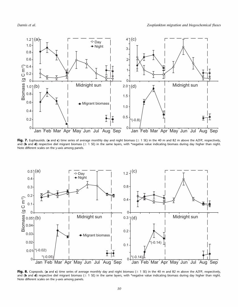
Diel migrant biomass from acoustic data
In the 2–40 m layer, the monthly mean of euphausiid
biomass was always higher at night than at day from January
to April, and from August to September (Fig. 7a). Euphausiid
biomass showed a first peak in February, with 0.9 g C m22 at
night, and a second peak of lesser magnitude in May–June
during the midnight sun and peak season of primary produc-
tion. The range of euphausiid biomass in January, estimated
from the MIK net sampling a few days before the onset of
synchronous DVM (0.09–0.6 g m22), is comparable with the
range derived from the AZFP data for the entire study period
(0.09–0.9 g m22). Likewise, night biomass estimates from the
MIK nets close to the September equinox (0.5–0.8 g m22)
were within the same range, whereas the estimates during
the day were much lower (0.0008–0.001 g m22). The
euphausiid migrant biomass, based on day-night change,
peaked in February–March (> 0.6 g C m22) and reached a
minimum in April (0.09 g C m22) close to the onset of mid-
night sun (Fig. 7b). The pattern in the 2–82 m layer was
somewhat different from the observations in 2–40 m (Fig.
7c). First, the mean biomass was higher during day than at
night in January, a bias likely due to DVM occurring essen-
tially over the top 40 m layer until late January. The second
peak of euphausiid biomass (3.2 g C m22) in the midst of
midnight sun in June was higher than the first winter peak
in March. Migrant biomass peaked in February–March,
remaining above 1 g C m22.
Classical DVM was also observed for copepods and chae-
tognaths prior to the onset of midnight sun and in August–
September in the 2–40 m layer (Figs. 8a, 9a). However, in the
darkest months of January and February, copepod biomass
tended to be higher at day than at night (Fig. 8a) and differ-
ence between night and day values was much less marked
for the copepod group than for euphausiids and chaetog-
naths. On the other hand, the latter two displayed similar
patterns, although the biomass estimates for the chaetog-
naths were much less.
Copepod and chaetognath biomass increased in the sur-
face layer in June, coinciding with the season of high prima-
ry production. Copepod biomass from AZFP data (0.2–0.3 g
m22) fell within the range of biomass values estimated from
mesozooplankton net sampling of the top 0–50 m layer in
January and September (0.02–0.2 g m22). For copepods, a
classic migrant biomass (shallower distribution at night and
Tim
e sp
ent a
t dep
th (h
)
0
5
10
15
20
Feb Mar Apr May Jun Jul AugJan
Not Determined
below 40 mbelow 80 m
Fig. 5. Time series of time spent below 40 m and 82 m depth by thehigh backscatter over a 24-h cycle from January to September 2014.The horizontal broken line indicates the 12-h limit.
Euphausiid Themisto spp. Chaetognath Other
0
Calanus spp. Calanus hyperboreus Metridia longa Pseudocalanus spp.Microcalanus spp. Chaetognath Other
0
0.4
1.2
1.4
1.8
Bio
mas
s (g
C m
-2)
JanuaryDay Night
SeptemberDay Night
MayDay Night
July
Macrozooplankton in 0-30 m layer
Mesozooplankton in 0-50 m layer
Mesozooplankton in 0-100 m layer
0.2
1.6
0
3.8
4.6
0.6
4.2
1.6
Not identified
n=5 n=4
n=2
n=2
n=2n=2
n=2n=2n=1 n=4
n=1
n=1
n=2
n=2
n=2n=2 n=1 n=4
0.2
0.4
0.6
0.8
1.0
0.8
5.0
Fig. 6. Macro- and mesozooplankton biomass and composition fromplankton net data in the surface 30-m, 50-m, and 100-m layer at day
and at night in January, May, July, and September 2014 at station KB3in Kongsfjorden. “n” indicates number of plankton net deployments.
Darnis et al. Zooplankton migration and biogeochemical fluxes
9
(a)
0
3
(c)
Jan Mar May Jul Sep
Bio
mas
s (g
C m
-2)
0Feb Apr Jun Aug Jan Mar May Jul Sep
0Feb Apr Jun Aug
0.5
1.0
*(-0.8)
(b) (d)
Migrant biomass
Midnight sun Midnight sun 0
0.21
1.5
2.0
0.4
0.6
0.8
1.01.2
0.2
0.4
0.6
0.8
1.0
DayNight
4
2
Fig. 7. Euphausiids. (a and c) time series of average monthly day and night biomass (6 1 SE) in the 40 m and 82 m above the AZFP, respectively,and (b and d) respective diel migrant biomass (6 1 SE) in the same layers, with *negative value indicating biomass during day higher than night.
Note different scales on the y-axis among panels.
0
1.2 (c)
Jan Mar May Jul Sep
Bio
mas
s (g
C m
-2)
0Feb Apr Jun Aug Jan Mar May Jul Sep
0Feb Apr Jun Aug
0.1
(b) (d)
Migrant biomass
Midnight sun Midnight sun 0
0.10.4
0.2
0.3
0.2
0.3
0.4
0.5
0.01
0.02
0.03
0.04
0.05
DayNight
0.8
(a)
*(-0.14)
*(-0.14)
*(-0.02)
*(-0.05)
Fig. 8. Copepods. (a and c) time series of average monthly day and night biomass (6 1 SE) in the 40 m and 82 m above the AZFP, respectively,and (b and d) respective diel migrant biomass (6 1 SE) in the same layers, with *negative value indicating biomass during day higher than night.
Note different scales on the y-axis among panels.
Darnis et al. Zooplankton migration and biogeochemical fluxes
10
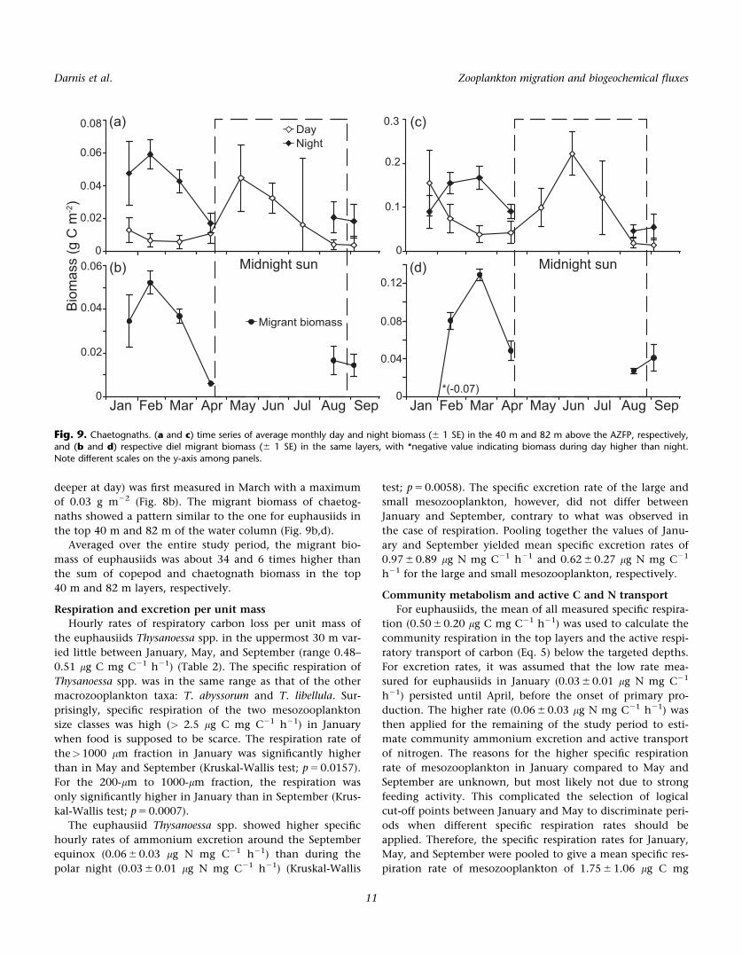
deeper at day) was first measured in March with a maximum
of 0.03 g m22 (Fig. 8b). The migrant biomass of chaetog-
naths showed a pattern similar to the one for euphausiids in
the top 40 m and 82 m of the water column (Fig. 9b,d).
Averaged over the entire study period, the migrant bio-
mass of euphausiids was about 34 and 6 times higher than
the sum of copepod and chaetognath biomass in the top
40 m and 82 m layers, respectively.
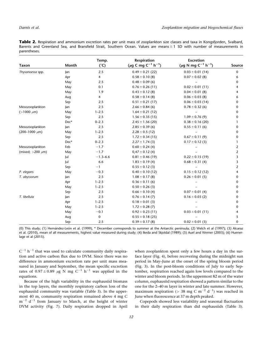
Respiration and excretion per unit mass
Hourly rates of respiratory carbon loss per unit mass of
the euphausiids Thysanoessa spp. in the uppermost 30 m var-
ied little between January, May, and September (range 0.48–
0.51 lg C mg C21 h21) (Table 2). The specific respiration of
Thysanoessa spp. was in the same range as that of the other
macrozooplankton taxa: T. abyssorum and T. libellula. Sur-
prisingly, specific respiration of the two mesozooplankton
size classes was high (> 2.5 lg C mg C21 h21) in January
when food is supposed to be scarce. The respiration rate of
the>1000 lm fraction in January was significantly higher
than in May and September (Kruskal-Wallis test; p 5 0.0157).
For the 200-lm to 1000-lm fraction, the respiration was
only significantly higher in January than in September (Krus-
kal-Wallis test; p 5 0.0007).
The euphausiid Thysanoessa spp. showed higher specific
hourly rates of ammonium excretion around the September
equinox (0.06 6 0.03 lg N mg C21 h21) than during the
polar night (0.03 6 0.01 lg N mg C21 h21) (Kruskal-Wallis
test; p 5 0.0058). The specific excretion rate of the large and
small mesozooplankton, however, did not differ between
January and September, contrary to what was observed in
the case of respiration. Pooling together the values of Janu-
ary and September yielded mean specific excretion rates of
0.97 6 0.89 lg N mg C21 h21 and 0.62 6 0.27 lg N mg C21
h21 for the large and small mesozooplankton, respectively.
Community metabolism and active C and N transport
For euphausiids, the mean of all measured specific respira-
tion (0.50 6 0.20 lg C mg C21 h21) was used to calculate the
community respiration in the top layers and the active respi-
ratory transport of carbon (Eq. 5) below the targeted depths.
For excretion rates, it was assumed that the low rate mea-
sured for euphausiids in January (0.03 6 0.01 lg N mg C21
h21) persisted until April, before the onset of primary pro-
duction. The higher rate (0.06 6 0.03 lg N mg C21 h21) was
then applied for the remaining of the study period to esti-
mate community ammonium excretion and active transport
of nitrogen. The reasons for the higher specific respiration
rate of mesozooplankton in January compared to May and
September are unknown, but most likely not due to strong
feeding activity. This complicated the selection of logical
cut-off points between January and May to discriminate peri-
ods when different specific respiration rates should be
applied. Therefore, the specific respiration rates for January,
May, and September were pooled to give a mean specific res-
piration rate of mesozooplankton of 1.75 6 1.06 lg C mg
0
0.3 (c)
Jan Mar May Jul Sep
Bio
mas
s (g
C m
-2)
0Feb Apr Jun Aug Jan Mar May Jul Sep
0Feb Apr Jun Aug
(b) (d)
Migrant biomass
Midnight sun Midnight sun 0
0.10.02
0.04
0.06
0.08
0.02
0.04
DayNight
0.2
(a)
0.04
0.08
0.12
*(-0.07)
0.06
Fig. 9. Chaetognaths. (a and c) time series of average monthly day and night biomass (6 1 SE) in the 40 m and 82 m above the AZFP, respectively,and (b and d) respective diel migrant biomass (6 1 SE) in the same layers, with *negative value indicating biomass during day higher than night.
Note different scales on the y-axis among panels.
Darnis et al. Zooplankton migration and biogeochemical fluxes
11
C21 h21 that was used to calculate community daily respira-
tion and active carbon flux due to DVM. Since there was no
difference in ammonium excretion rate per unit mass mea-
sured in January and September, the mean specific excretion
rates of 0.97 6 0.89 lg N mg C21 h21 was applied in the
equations.
Because of the high variability in the euphausiid biomass
in the top layers, the monthly respiratory carbon loss of the
euphausiid community was variable (Table 3). In the upper-
most 40 m, community respiration remained above 4 mg C
m22 d21 from January to March, at the height of winter
DVM activity (Fig. 7). Daily respiration dropped in April
when zooplankton spent only a few hours a day in the sur-
face layer (Fig. 4), before recovering during the midnight sun
period in May–June at the onset of the spring bloom period
(Fig. 3). In the post-bloom conditions of July to early Sep-
tember, respiration reached again low levels compared to the
winter and bloom periods. In the uppermost 82 m of the water
column, euphausiid respiration showed a pattern similar to the
one for the 2–40 m layer in winter and late summer. However,
maximum respiration (> 38 mg C m22 d21) was reached in
June when fluorescence at 37 m depth peaked.
Copepods showed less variability and seasonal fluctuation
in their daily respiration than did euphausiids (Table 3).
Table 2. Respiration and ammonium excretion rates per unit mass of zooplankton size classes and taxa in Kongsfjorden, Svalbard,Barents and Greenland Sea, and Bransfield Strait, Southern Ocean. Values are means 6 1 SD with number of measurements inparentheses.
Taxon Month
Temp. Respiration Excretion
Source(8C) (lg C mg C21 h21) (lg N mg C21 h21)
Thysanoessa spp. Jan 2.5 0.49 6 0.21 (22) 0.03 6 0.01 (14) 0
Apr 4 0.58 6 0.10 (8) 0.07 6 0.02 (8) 6
May 2.5 0.48 6 0.09 (6) – 0
May 0.1 0.76 6 0.26 (11) 0.02 6 0.01 (11) 4
May 1.9 0.43 6 0.12 (8) 0.04 6 0.01 (8) 4
Aug 4 0.58 6 0.14 (8) 0.06 6 0.03 (8) 6
Sep 2.5 0.51 6 0.21 (17) 0.06 6 0.03 (14) 0
Mesozooplankton Jan 2.5 2.66 6 0.84 (6) 0.78 6 0.32 (6) 0
(>1000 lm) May 1–2.5 1.64 6 0.21 (12) – 0
Sep 2.5 1.56 6 0.35 (15) 1.09 6 0.76 (9) 0
Dec* 0–2.3 2.45 6 1.56 (20) 0.38 6 0.16 (20) 1
Mesozooplankton Jan 2.5 2.85 6 0.39 (6) 0.55 6 0.11 (6) 0
(200–1000 lm) May 1–2.5 2.28 6 0.5 (12) – 0
Sep 2.5 1.72 6 0.34 (15) 0.67 6 0.11 (9) 0
Dec* 0–2.3 2.27 6 1.74 (3) 0.17 6 0.12 (3) 1
Mesozooplankton Feb 21.7 0.60 6 0.24 (4) – 2
(mixed; >200 lm) May 21.7 0,47 6 0.12 (4) – 2
Jul 21.3–6.6 0.81 6 0.46 (19) 0.22 6 0.15 (19) 3
Jul 6.6 1.83 6 0.19 (4) 0.68 6 0.31 (4) 3
Sep 21 0.55 6 0.12 (3) – 2
P. elegans May 20.3 0.40 6 0.10 (12) 0.15 6 0.12 (12) 4
T. abyssorum Jan 2.5 1.08 6 0.17 (8) 0.26 6 0.01 (5) 0
Apr 1–2.5 0.36 6 0.11 (6) – 0
May 1–2.5 0.50 6 0.26 (3) – 0
Sep 2.5 0.66 6 0.10 (4) 0.07 6 0.01 (4) 0
T. libellula Jan 2.5 0.76 6 0.14 (7) 0.16 6 0.03 (2) 0
Apr 1–2.5 0.18 6 0.01 (3) – 0
May 1–2.5 1.72 6 0.28 (7) – 0
May 20.1 0.92 6 0.23 (11) 0.03 6 0.01 (11) 4
Aug 0 0.55 6 0.18 (25) – 5
Sep 2.5 0.39 6 0.17 (8) 0.02 6 0.01 (3) 0
(0) This study; (1) Hern�andez-Le�on et al. (1999), * December corresponds to summer at the Antarctic peninsula; (2) Welch et al (1997); (3) Alcaraz
et al. (2010), mean of all measurements, highest value measured during study; (4) Ikeda and Skjoldal (1989); (5) Auel and Werner (2003); (6) Huener-lage et al (2015).
Darnis et al. Zooplankton migration and biogeochemical fluxes
12
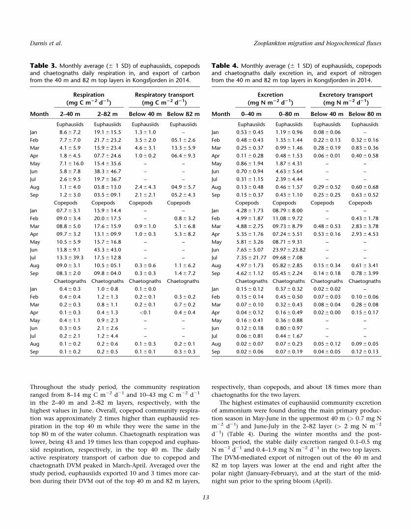
Throughout the study period, the community respiration
ranged from 8–14 mg C m22 d21 and 10–43 mg C m22 d21
in the 2–40 m and 2–82 m layers, respectively, with the
highest values in June. Overall, copepod community respira-
tion was approximately 2 times higher than euphausiid res-
piration in the top 40 m while they were the same in the
top 80 m of the water column. Chaetognath respiration was
lower, being 43 and 19 times less than copepod and euphau-
siid respiration, respectively, in the top 40 m. The daily
active respiratory transport of carbon due to copepod and
chaetognath DVM peaked in March-April. Averaged over the
study period, euphausiids exported 10 and 3 times more car-
bon during their DVM out of the top 40 m and 82 m layers,
respectively, than copepods, and about 18 times more than
chaetognaths for the two layers.
The highest estimates of euphausiid community excretion
of ammonium were found during the main primary produc-
tion season in May-June in the uppermost 40 m (> 0.7 mg N
m22 d21) and June-July in the 2–82 layer (> 2 mg N m22
d21) (Table 4). During the winter months and the post-
bloom period, the stable daily excretion ranged 0.1–0.5 mg
N m22 d21 and 0.4–1.9 mg N m22 d21 in the two top layers.
The DVM-mediated export of nitrogen out of the 40 m and
82 m top layers was lower at the end and right after the
polar night (January-February), and at the start of the mid-
night sun prior to the spring bloom (April).
Table 3. Monthly average (6 1 SD) of euphausiids, copepodsand chaetognaths daily respiration in, and export of carbonfrom the 40 m and 82 m top layers in Kongsfjorden in 2014.
Respiration
(mg C m22 d21)
Respiratory transport
(mg C m22 d21)
Month 2–40 m 2–82 m Below 40 m Below 82 m
Euphausiids Euphausiids Euphausiids Euphausiids
Jan 8.6 6 7.2 19.1 6 15.5 1.3 6 1.0 –
Feb 7.7 6 7.0 21.7 6 23.2 3.5 6 2.0 05.1 6 2.6
Mar 4.1 6 5.9 15.9 6 23.4 4.6 6 3.1 13.3 6 5.9
Apr 1.8 6 4.5 07.7 6 24.6 1.0 6 0.2 06.4 6 9.3
May 7.1 6 16.0 15.4 6 35.6 – –
Jun 5.8 6 7.8 38.3 6 46.7 – –
Jul 2.6 6 9.5 19.7 6 36.7 – –
Aug 1.1 6 4.0 03.8 6 13.0 2.4 6 4.3 04.9 6 5.7
Sep 1.2 6 3.0 03.5 6 09.1 2.1 6 2.1 05.2 6 4.3
Copepods Copepods Copepods Copepods
Jan 07.7 6 3.1 15.9 6 14.4 – –
Feb 09.0 6 3.4 20.0 6 17.5 – 0.8 6 3.2
Mar 08.8 6 5.0 17.6 6 15.9 0.9 6 1.0 5.1 6 6.8
Apr 09.7 6 3.2 13.1 6 09.9 1.0 6 0.3 5.3 6 8.2
May 10.5 6 5.9 15.7 6 16.8 – –
Jun 13.8 6 9.1 43.3 6 43.0 – –
Jul 13.3 6 39.3 17.5 6 12.8 – –
Aug 09.0 6 3.1 10.5 6 05.1 0.3 6 0.6 1.1 6 6.2
Sep 08.3 6 2.0 09.8 6 04.0 0.3 6 0.3 1.4 6 7.2
Chaetognaths Chaetognaths Chaetognaths Chaetognaths
Jan 0.4 6 0.3 1.0 6 0.8 0.1 6 0.0
Feb 0.4 6 0.4 1.2 6 1.3 0.2 6 0.1 0.3 6 0.2
Mar 0.2 6 0.3 0.8 6 1.1 0.2 6 0.1 0.7 6 0.2
Apr 0.1 6 0.3 0.4 6 1.3 <0.1 0.4 6 0.4
May 0.4 6 1.1 0.9 6 2.3 – –
Jun 0.3 6 0.5 2.1 6 2.6 – –
Jul 0.2 6 2.1 1.2 6 4.4 – –
Aug 0.1 6 0.2 0.2 6 0.6 0.1 6 0.3 0.2 6 0.1
Sep 0.1 6 0.2 0.2 6 0.5 0.1 6 0.1 0.3 6 0.3
Table 4. Monthly average (6 1 SD) of euphausiids, copepodsand chaetognaths daily excretion in, and export of nitrogenfrom the 40 m and 82 m top layers in Kongsfjorden in 2014.
Excretion
(mg N m22 d21)
Excretory transport
(mg N m22 d21)
Month 0–40 m 0–80 m Below 40 m Below 80 m
Euphausiids Euphausiids Euphausiids Euphausiids
Jan 0.53 6 0.45 1.19 6 0.96 0.08 6 0.06 –
Feb 0.48 6 0.43 1.35 6 1.44 0.22 6 0.13 0.32 6 0.16
Mar 0.25 6 0.37 0.99 6 1.46 0.28 6 0.19 0.83 6 0.36
Apr 0.11 6 0.28 0.48 6 1.53 0.06 6 0.01 0.40 6 0.58
May 0.86 6 1.94 1.87 6 4.31 – –
Jun 0.70 6 0.94 4.63 6 5.64 – –
Jul 0.31 6 1.15 2.39 6 4.44 – –
Aug 0.13 6 0.48 0.46 6 1.57 0.29 6 0.52 0.60 6 0.68
Sep 0.15 6 0.37 0.43 6 1.10 0.25 6 0.25 0.63 6 0.52
Copepods Copepods Copepods Copepods
Jan 4.28 6 1.73 08.79 6 8.00 – –
Feb 4.99 6 1.87 11.08 6 9.72 – 0.43 6 1.78
Mar 4.88 6 2.75 09.73 6 8.79 0.48 6 0.53 2.83 6 3.78
Apr 5.35 6 1.76 07.24 6 5.51 0.53 6 0.16 2.93 6 4.53
May 5.81 6 3.26 08.71 6 9.31 – –
Jun 7.65 6 5.07 23.97 6 23.82 – –
Jul 7.35 6 21.77 09.68 6 7.08 – –
Aug 4.97 6 1.73 05.82 6 2.85 0.15 6 0.34 0.61 6 3.41
Sep 4.62 6 1.12 05.45 6 2.24 0.14 6 0.18 0.78 6 3.99
Chaetognaths Chaetognaths Chaetognaths Chaetognaths
Jan 0.15 6 0.12 0.37 6 0.32 0.02 6 0.02 –
Feb 0.15 6 0.14 0.45 6 0.50 0.07 6 0.03 0.10 6 0.06
Mar 0.07 6 0.10 0.32 6 0.43 0.08 6 0.04 0.28 6 0.08
Apr 0.04 6 0.12 0.16 6 0.49 0.02 6 0.00 0.15 6 0.17
May 0.16 6 0.41 0.36 6 0.88 – –
Jun 0.12 6 0.18 0.80 6 0.97 – –
Jul 0.06 6 0.81 0.44 6 1.67 – –
Aug 0.02 6 0.07 0.07 6 0.23 0.05 6 0.12 0.09 6 0.05
Sep 0.02 6 0.06 0.07 6 0.19 0.04 6 0.05 0.12 6 0.13
Darnis et al. Zooplankton migration and biogeochemical fluxes
13
Copepod daily excretion of ammonium was about 14 and
6 times the euphausiid excretion in the 2–40 m and 2–82 m
surface layers, respectively. Copepod excretion reached a
maximum in June with a steep peak in the 2–82 m layer
(24 mg N m22 d21). Active export of N due to copepod DVM
culminated in March-April. On average, copepods trans-
ported 30% more N out of uppermost 40 m than euphau-
siids and 4 times more from the 2–82 m layer during the
winter period. On the other hand, euphausiids exported 30%
more and 6% less N than copepods did from the same two
layers, respectively, during the post-bloom period. In com-
parison with euphausiids and copepods, chaetognaths had
lower excretion rates that were never>0.8 mg N m22 d21 in
the two studied layers. Their capacity to transport N below
these layers was thus low compared to the two other zoo-
plankton groups.
Sinking flux of POC and PON
Sinking POC flux integrated over the winter period 21
January–3 April was 0.7 g m22 at 40 m depth in 2014, and
2.1 g m22 at 100 m depth in 2013. Over the period 9
August–6 September, similar in duration to the autumn
DVM period sampled in our study (11 August–9 September),
the POC flux was 0.7 g m22 at 100 m depth in 2013.
In the same winter period as above, the sinking PON flux
was 0.25 g m22 at 40 m depth in 2014, and 0.37 g m22 at
100 m depth in 2013. In the autumn period, the PON flux
was 0.12 g m22 at 100 m depth in 2013.
Discussion
Seasonal variability in DVM
The visual analysis of the data from the moored AZFP
multifrequency echosounder identified classical DVM from
the end of January to mid-April, and recorded the onset of
autumn DVM in mid-August (Fig. 3). Previous observations
at the same site based on ADCP data collected from 2006 to
2008 suggest that the autumn DVM period lasted until mid-
November (Wallace et al. 2010), which would make the two
DVM phases equal in duration. During the DVM periods,
zooplankton moved synchronously in and out of the upper-
most layer of the water column over depth ranges of 40 m
(depth of sediment traps) and 82 m (deepest threshold sam-
pled by the AZFP) that are relevant for vertical fluxes of ele-
ments. Covering almost the entire water column, the ADCP
echogram in late September showed DVM amplitudes of
120–140 m at the autumn equinox (Fig. 4). The two periods
of classical synchronous DVM were out of phase with the
period of high pelagic primary productivity, most probably
reducing the contribution of active transport to the biologi-
cal pump. Such uncoupling between DVM and the phyto-
plankton bloom was also observed in 2007 and 2008 in
Kongsfjorden (Wallace et al. 2010), and this pattern is likely
the rule rather than the exception in high-Arctic ecosystems.
Here, there is generally a single bloom, usually between late
April and August (Daase et al. 2013), and during a period of
reduced diel light variation due to midnight sun. With the
ongoing loss of Arctic sea ice, many regions at the periphery
of the shrinking perennial ice pack are developing a second
bloom in the autumn (Ardyna et al. 2014), and it is likely
that this will coincide with the autumn DVM phase. Thus,
we can expect classic DVM to have a growing role in the bio-
logical pump if these observed changes in phytoplankton
seasonality amplify in the future.
Combining the AZFP data analysis with morphometric
information on zooplankton caught in nets allowed us to
identify euphausiids as the major diel migrants in terms of
biomass in the fjord in 2014. This finding was further vali-
dated with plankton net data limited to January and Septem-
ber that showed that euphausiids of the genus Thysanoessa
made up the bulk of macrozooplankton biomass (> 90%) at
night. We also attributed the high backscatter in the surface
layer in June to the presence of Thysanoessa spp., although
macrozooplankton were not sampled quantitatively with
nets during the spring-summer season due to the unavail-
ability of a ship large enough for trawling large plankton
nets. Temperature profiles above 28C throughout the water
column in May and July revealed no significant intrusion of
cold Arctic Water into Kongsfjorden. Furthermore, mesozoo-
plankton data from the same period indicate no change in
the community that could have signaled a massive advec-
tion of Arctic zooplankton. Thus, we assumed that the mac-
rozooplankton size class, dominated by the arcto-boreal
Thysanoessa spp. during winter, did not shift either to a
more Arctic assemblage during the period of high biological
production. It is possible, however, that larger macrozoo-
plankton like the more Atlantic Meganyctiphanes norvegica
were underestimated in the net samples as they could possi-
bly avoid the net type and trawl short duration used.
Large copepods (dominated by Calanus spp.) and chaetog-
naths (essentially P. elegans) also performed diel migrations
during the two DVM periods. Nevertheless, zooplankton bio-
mass derived from the calibrated AZFP revealed that euphau-
siids generally contributed>90% of the total diel migrant
biomass (euphausiids 1 copepods 1 chaetognaths) in the
uppermost 40 m and 82 m. The unverified assumption of a
monospecific zooplankton assemblage in each echo-
integration cell of the acoustic analysis may have had an
effect on the estimation of biomass that is difficult to evalu-
ate. However, we are confident that the small size selected
for the cells (1-m vertical by 5-min horizontal) tempers this
effect. The daily zooplankton migrant biomass below 82 m
during the transition from polar night to midnight sun and
in late summer in Kongsfjorden exceeded most of the esti-
mates for other systems where active fluxes due to DVM
were studied (Supporting Information Table S3). Our range
of estimates did encompass the higher values measured off
the Canary Islands and in the North Pacific (Yebra et al.
Darnis et al. Zooplankton migration and biogeochemical fluxes
14
2005; Steinberg et al. 2008; Takahashi et al. 2009). One of
the plausible reasons for the discrepancy between our high
estimates and those of other studies is that most of these
others did not include the macrozooplankton size class,
which dominated zooplankton migrant biomass in Kongsf-
jorden. Therefore, their assessment of the importance of zoo-
plankton active fluxes of carbon and nitrogen may well be
very conservative.
Zooplankton metabolism
This study significantly expands on the limited knowl-
edge of respiration and ammonium excretion rates of arctic
euphausiids. The mass-specific respiration rates of Thysa-
noessa spp. (mainly T. inermis) in winter, spring and autumn
2014 were close to the value found in April (pre-bloom peri-
od) and August (post-bloom) for T. inermis in Kongsfjorden
(Huenerlage et al. 2015), and within the range of values in
late May in the eastern Barents Sea (Ikeda and Skjoldal
1989). We did not observe a lower specific respiration during
the polar night period of food scarcity compared to the pre-
bloom period or to the autumn equinox, supporting the sug-
gestion of Huenerlage et al. (2015) that Thysanoessa spp. do
not reduce their metabolism in winter. It is possible that res-
piration rates were higher during the bloom period, between
late May and June, when the mainly herbivore T. inermis
ingests large quantities of pelagic algae to build its lipid
reserves. If so, our estimates of euphausiid community respi-
ration for the summer period would be conservative. Mass-
specific ammonium-excretion rates of Thysanoessa spp. in
our study are consistent with those measured by Ikeda and
Skjoldal (1989) and Huenerlage et al. (2015). The lower
excretion rate in January than in September is presumably
due to better feeding conditions in autumn, as excretion and
ingestion rates are closely linked (Saborowski et al. 2002).
Overall, mesozooplankton respiration rates reported here
are consistent with measurements on the same size classes
during the Antarctic summer (Hern�andez-Le�on et al. 1999),
and the highest value measured on total mesozooplankton
(not size-fractionated) from north-Svalbard in summer
(Alcaraz et al. 2010). But we measured higher mass-specific
respiration rates than Welch et al. (1997) did in the colder
waters of the Canadian Arctic archipelago. Likewise, meso-
zooplankton ammonium excretion rates in Kongsfjorden
were 1–3.5 times higher than the rates for Antarctica and
north-Svalbard (Table 2).
Pelagic primary production estimates in Kongsfjorden are
scarce and not available for 2014. Hodal et al. (2012) calcu-
lated a gross primary production (GPP) of 27–35 g C m22 in
the 0–40 m layer during the spring bloom of 2002 (18 April–
13 May), consistent with previous annual GPP estimates of
25–30 g C m22 in the northeast Barents Sea (Hegseth 1998).
Thus, assuming the same range of GPP in 2014 as in 2002,
euphausiids would have used 0.7–0.9% and large copepods
1.3–1.7% of the phytoplankton carbon produced to cover
their respiratory carbon loss (Rc) during the bloom, here cir-
cumscribed to 15 May–20 June. These fractions are much
less than the 5–67% (average 23%) of GPP that mesozoo-
plankton respiration alone accounted for in the northwest
Barents Sea (Alcaraz et al. 2010). However, it is important to
bear in mind that our metabolic measurements were not
made during bloom conditions and, thus, are likely underes-
timates of respiration and excretion during the bloom peri-
od. A rough estimate of zooplankton ingestion (I), using the
equation of Ikeda and Motoda (1978) in which I 5 2.5 Rc,
shows that combined euphausiid-copepod grazing would
account for 5–6% of GPP, a range below the 22–44% of GPP
intercepted by zooplankton in the northeast Barents Sea
(Wexels Riser et al. 2008), or 45% by copepods in the Green-
land Northeast Water Polynya (Daly 1997). Using the Red-
field ratio to convert phytoplankton carbon production to
nitrogen production, euphausiid and mesozooplankton
NH41 excretion in the uppermost 40 m would support 5–7%
of the bloom GPP. This is again low compared to the 9–
242% (mean 59%) that mesozooplankton alone re-supplied
in the photic layer of the northern Barents Sea for phyto-
plankton production in July (Alcaraz et al. 2010). Therefore,
we suggest that the effect of zooplankton grazing and excre-
tion on phytoplankton total production was weak in Kongsf-
jorden during the bloom of 2014.
Active export of dissolved carbon and nitrogen mediated
by DVM
The active transport of carbon due to synchronous migra-
tion by euphausiids, large copepods and chaetognaths was
0.3 g m22 and 0.9 g m22 below 40 m and 82 m depth,
respectively, during the 2014 winter DVM period in Kongsf-
jorden (31 January–11 April), and 0.2 g m22 below 82 m at
the onset of the autumn DVM (from 11 August to 9 Septem-
ber). Thus, the DVM-mediated carbon transport would repre-
sent>40% of the winter carbon sinking flux of POC
measured in sediment traps, and>25% of the sinking flux
during the first weeks of autumn. These ratios of active to
passive carbon export fall within the range of ratios for daily
fluxes (13–70%) in several oligotrophic and more seasonally
stable sub-Arctic to equatorial systems (Dam et al. 1995;
Zhang and Dam 1997; Hern�andez-Le�on et al. 2001; Yebra
et al. 2005; Stukel et al. 2013) (Supporting Information Table
S3). Representing >25% of POC sinking flux, the DVM
transport in Kongsfjorden was higher than other estimates
(1–14% of sinking flux) for different times of the year in the
subtropical Atlantic, Bermuda, around the Canary Islands,
and from equatorial to subarctic Pacific regions (Le Borgne
and Rodier 1997; Rodier and Le Borgne 1997; Kobari et al.
2008; Putzeys et al. 2011). The 0.9 g C m22 transported by
winter DVM in Kongsfjorden represents 30% of the active
flux by Calanus spp. (mainly C. hyperboreus) SVM below
100 m (3.1 g C m22) during the overwintering period (Octo-
ber–April) in the southeastern Beaufort Sea (Darnis and
Darnis et al. Zooplankton migration and biogeochemical fluxes
15
Fortier 2012). Adding the amount transported to depth by
autumn DVM could possibly double the contribution of
DVM-mediated transport over an annual cycle. Using short-
term sediment trap deployments (21–52 h) in Kongsfjorden
in 2012–2013, Lalande et al. (2016) provide three estimates
of daily sinking POC fluxes: during a bloom in May, and
post-bloom conditions in August and October (Supporting
Information Table S5). Comparison between daily active
transport below 82 m and the mean post-bloom POC flux in
2012 (167 6 88 mg C m22 d21 at 100 m) yields active to pas-
sive export ratios from 4–12% that are within the range of
low ratios published. To estimate the active transports, the
zooplankton groups were assumed not to feed at depth. This
may have been the case for copepods and euphausiids but
not for the carnivorous chaetognaths. However, the latter
represented a minor fraction of the migrant biomass.
Although not ideal, such comparisons involving different
years, locations, and seasons reveal all the same that, despite
the complex DVM regime at high latitudes, the active car-
bon transport due to DVM in Kongsfjorden is close to what
has been reported in lower latitude regions of the World
Ocean.
Zooplankton winter DVM transported 0.03 g N m22 and
0.18 g N m22 out of the 40 m and 82 m top water layers,
respectively, whereas early autumn DVM transported 0.04 g
N m22 out the 100 m top layer. The DVM-mediated active
transport of nitrogen represents thus 12% and 49% of the
PON sinking flux at 40 m and 100 m integrated over the
winter period, and 33% of the sinking flux at 100 m in early
autumn. Such ratios of active to passive export of nitrogen
fall well within the wide range of ratios (7–108% of daily
PON flux) stemming from the few studies addressing active
transport of nitrogen due to DVM (Longhurst and Harrison
1988; Longhurst et al. 1989; Al-Mutairi and Landry 2001;
Steinberg et al. 2002) (Supporting Information Table S4). On
a daily basis, however, estimates of active N transport due to
euphausiid, copepod, and chaetognath represent 4–18% of
the mean sinking flux of PON (21 6 7 mg N m22 d21) below
100 m during the post-bloom conditions in 2012 (Support-
ing Information Table S5). Our daily ratios thus lie at the
lower range of published ratios. Interestingly, winter DVM
and excretion at depth by large copepods contributed 76%
of the active N transport, whereas it was euphausiid DVM
and their respiration at depth that dominated in similar pro-
portion (70%) the active C transport during the same period.
By using acoustic data with measurements of respiration
and ammonium excretion, we have been able to describe for
the first time the role of zooplankton DVM in the function-
ing of the biological pump of a high-latitude marine ecosys-
tem. As expected, the active transport of carbon and
nitrogen to depth through synchronous DVM is discontinu-
ous over an annual cycle, due to the suspension of DVM
during parts of the polar night and midnight sun (Cottier
et al. 2006; Berge et al. 2009; Last et al. 2016). The fact that
this process occurs essentially outside of the short season of
high photosynthesis likely limits its function in the biologi-
cal pump of Arctic ecosystems if an annual budget is to be
estimated. On the other hand, this study also revealed that
the importance of active transport in the Kongsfjorden eco-
system during times of strong DVM (winter and autumn)
compared well with other oceanic systems. Since the winter
DVM took place in a fully mixed water column in Kongsfjor-
den, the active transports estimated for winter cannot be
regarded as export fluxes. But at other times of the year
(Loeng 1991) and in other locations in the Arctic, DVM
coincides with highly stratified water columns. Production
of sinking fecal pellets, active transport of feces in the
migrants’ guts, high winter mortality at depth, and shedding
of exuviae, should also be quantified and included in C and
N budgets along with DVM-mediated flux of dissolved com-
ponents measured here. If we are to achieve a realistic
description of the biological pump of the Arctic marine eco-
systems, it will be especially important to estimate these
rates during the understudied periods outside of the short
spring-summer season. Based on our results, it remains that
respiratory C and excretory N transport due to DVM should
be considered for flux estimation in the extensive Arctic
regions permanently subject to haline stratification. Under
the effect of global warming, the increased river runoff and
sea ice melt will result in a better match in timing between
DVM-mediated processes and stratification of the water col-
umn (Pemberton and Nilsson 2016), which should increase
the efficiency of the biological carbon pump. Furthermore,
Cottier et al. (2006) and Wallace et al. (2010) found evidence
for unsynchronized migration in Kongsfjorden during the
midnight sun in June. Zooplankton would swim individually
in the surface layer, possibly to feed, and sink out during
digestion repeatedly over a 24-h period. In 2014, June coin-
cided with maximum fluorescence and zooplankton biomass
in the 82 m surface layer. Direct vertical shunting of carbon
and nitrogen to deeper less retentive layers due to this foray-
type migration would enhance the efficiency of the biologi-
cal pump when biological productivity is at its highest. How-
ever, unsynchronized migration needs to be investigated in
other high-latitude regions. For instance, no unsynchronized
migrations were detected during the midnight sun in the
Antarctic Weddell Sea (Cisewski and Strass 2016) and over
the West Spitsbergen outer shelf (Geoffroy et al. 2016).
The finding of the prominent role of euphausiids (particu-
larly Thysanoessa spp.) in the active vertical transport of car-
bon has also been reported lately in the North-west
Mediterranean Sea (Isla et al. 2015). Euphausiids are abun-
dant in the shelf seas on the Pacific side of the Arctic as well
(Eisner et al. 2013) where there is a stronger stratification of
the water column. Over the Arctic continental slopes and
basins, little is known about the distribution of macrozoo-
plankton and it is assumed so far that long-range SVM by
large C. hyperboreus is the main pathway for the active
Darnis et al. Zooplankton migration and biogeochemical fluxes
16
vertical flux of carbon (Hirche 1997; Darnis and Fortier
2012). To be able to fully assess the function of zooplankton
migrations in the biological pump on a pan-Arctic scale, we
need to define better the biogeography, feeding biology, and
migratory parameters (depth range, swimming speed, time at
depth) of key zooplankton taxa, namely the Arctic Calanus
spp., the arcto-boreal Thysanoessa spp. and other macrozoo-
plankton like Themisto spp.
References
Alcaraz, M., and others. 2010. The role of arctic zooplankton
in biogeochemical cycles: Respiration and excretion of
ammonia and phosphate during summer. Polar Biol. 33:
1719–1731. doi:10.1007/s00300-010-0789-9
Al-Mutairi, H., and M. R. Landry. 2001. Active export of car-
bon and nitrogen at Station ALOHA by diel migrant zoo-
plankton. Deep-Sea Res. Part II 48: 2083–2103. doi:
10.1016/S0967-0645(00)00174-0
Ardyna, M., M. Babin, M. Gosselin, E. Devred, L. Rainville,
and J. Tremblay. 2014. Recent Arctic Ocean sea ice loss
triggers novel fall phytoplankton blooms. Geophys. Res.
Lett. 41: 6207–6212. doi:10.1002/2014GL061047
ASL. 2014. AZFP (Acoustic Zooplankton Fish Profiler) opera-
tors manual, p. 77. ASL.
Auel, H., and I. Werner. 2003. Feeding, respiration and life
history of the hyperiid amphipod Themisto libellula in the
Arctic marginal ice zone of the Greenland Sea.. J. Exp.
Mar. Biol. Ecol. 296: 183–197.
Basedow, S. L., K. Eiane, V. Tverberg, and M. Spindler. 2004.
Advection of zooplankton in an Arctic fjord (Kongsfjor-
den, Svalbard). Estuar. Coast. Shelf Sci. 60: 113–124. doi:
10.1016/j.ecss.2003.12.004
Benfield, M. C., C. S. Davis, and S. M. Gallager. 2000. Esti-
mating the in-situ orientation of Calanus finmarchicus on
Georges Bank using the Video Plankton Recorder. Plank-
ton Biol. Ecol. 47: 69–72.
Berge, J., and others. 2009. Diel vertical migration of Arctic
zooplankton during the polar night. Biol. Lett. 5: 69–72.
doi:10.1098/rsbl.2008.0484
Berge, J., and others. 2014. Arctic complexity: A case study
on diel vertical migration of zooplankton. J. Plankton Res.
36: 1279–1297. doi:10.1093/plankt/fbu059
Berge, J., and others. 2015. In the dark: A review of ecosys-
tem processes during the Arctic polar night. Prog. Ocean-
ogr. 139: 258–271. doi:10.1016/j.pocean.2015.08.005
Brierley, A. S. 2014. Diel vertical migration. Curr. Biol. 24:
R1074–R1076. doi:10.1016/j.cub.2014.08.054
Bronk, D. A., and D. K. Steinberg. 2008. Chapter 8 - nitrogen
regeneration, p. 385–467. In D. G. Capone, D. A. Bronk,
M. R. Mulholland, and E. J. Carpenter [eds.], Nitrogen in
the marine environment, 2nd ed. Academic Press.
Chu, D., K. G. Foote, and T. K. Stanton. 1993. Further analy-
sis of target strength measurements of Antarctic krill at 38
and 120 kHz: Comparison with deformed cylinder model
and inference of orientation distribution. J. Acoust. Soc.
Am. 93: 2985–2988. doi:10.1121/1.405818
Cisewski, B., and V. H. Strass. 2016. Acoustic insights into
the zooplankton dynamics of the eastern Weddell Sea.
Prog. Oceanogr. 144: 62–92. doi:10.1016/
j.pocean.2016.03.005
Cottier, F., V. Tverberg, M. Inall, H. Svendsen, F. Nilsen, and
C. Griffiths. 2005. Water mass modification in an Arctic
fjord through cross-shelf exchange: The seasonal hydrog-
raphy of Kongsfjorden, Svalbard. J. Geophys. Res. 110:
C12005. doi:10.1029/2004JC002757
Cottier, F. R., G. A. Tarling, A. Wold, and S. Falk-Petersen.
2006. Unsynchronized and synchronized vertical migra-
tion of zooplankton in a high Arctic fjord. Limnol. Oce-
anogr. 51: 2586–2599. doi:10.4319/lo.2006.51.6.2586
Cottier, F. R., F. Nilsen, M. E. Inall, S. Gerland, V. Tverberg,
and H. Svendsen. 2007. Wintertime warming of an Arctic
shelf in response to large-scale atmospheric circulation.
Geophys. Res. Lett. 34: L10607. doi:10.1029/
2007GL029948
Cottier, F. R., F. Nilsen, R. Skogseth, V. Tverberg, J.
Skarðhamar, and H. Svendsen. 2010. Arctic fjords: A
review of the oceanographic environment and dominant
physical processes. Geol. Soc. London Spec. Publ. 344:
35–50. doi:10.1144/SP344.4
Daase, M., K. Eiane, D. L. Aksnes, and D. Vogedes. 2008. Ver-
tical distribution of Calanus spp. and Metridia longa at
four Arctic locations. Mar. Biol. Res. 4: 193–207. doi:
10.1080/17451000801907948
Daase, M., and others. 2013. Timing of reproductive events
in the marine copepod Calanus glacialis: A pan-Arctic per-
spective. Can. J. Fish. Aquat. Sci. 70: 871–884. doi:
10.1139/cjfas-2012-0401
Daly, K. L. 1997. Flux of particulate matter through cope-
pods in the Northeast water polynya. J. Mar. Syst. 10:
319–342. doi:10.1016/S0924-7963(96)00062-0
Dam, H. G., M. R. Roman, and M. J. Youngbluth. 1995.
Downward export of respiratory carbon and dissolved
inorganic nitrogen by diel-migrant mesozooplankton at
the JGOFS Bermuda time-series station. Deep-Sea Res. Part
I 42: 1187–1197. doi:10.1016/0967-0637(95)00048-B
Darnis, G., and L. Fortier. 2012. Zooplankton respiration and
the export of carbon at depth in the Amundsen Gulf (Arc-
tic Ocean). J. Geophys. Res. 117: C04013. doi:10.1029/
2011JC007374
Ducklow, H. W., D. K. Steinberg, and K. O. Buesseler. 2001.
Upper ocean carbon export and the biological pump.
Oceanography 14: 50–58. doi:10.5670/oceanog.2001.06
Eisner, L., N. Hillgruber, E. Martinson, and J. Maselko. 2013.
Pelagic fish and zooplankton species assemblages in rela-
tion to water mass characteristics in the northern Bering
and southeast Chukchi seas. Polar Biol. 36: 87–113. doi:
10.1007/s00300-012-1241-0
Darnis et al. Zooplankton migration and biogeochemical fluxes
17
Fischer, J., and M. Visbeck. 1993. Seasonal variation of the
daily zooplankton migration in the Greenland Sea. Deep-
Sea Res. Part I Oceanogr. Res. Pap. 40: 1547–1557. doi:
10.1016/0967-0637(93)90015-U
Fortier, M., L. Fortier, H. Hattori, H. Saito, and L. Legendre.
2001. Visual predators and the diel vertical migration of
copepods under Arctic sea ice during the midnight sun. J.
Plankton Res. 23: 1263–1278. doi:10.1093/plankt/
23.11.1263
Geoffroy, M., F. R. Cottier, J. Berge, and M. E. Inall. 2016.
AUV-based acoustic observations of the distribution and
patchiness of pelagic scattering layers during midnight
sun. ICES J. Mar. Sci. (Special issue 6th Zooplankton Pro-
duction Symposium) doi:10.1093/icesjms/fsw158.
Gnaiger, E. 1983. Calculation of energetic and biochemical
equivalents of respiratory oxygen consumption, p. 337–
345. In E. Gnaiger and H. Forstner [eds.], Polarographic
oxygen sensors: Aquatic and physiological applications.
Springer-Verlag.
Hegseth, E. N. 1998. Primary production of the northern
Barents Sea. Polar Res. 17: 113–123. doi:10.1111/j.1751-
8369.1998.tb00266.x
Hegseth, E. N., and V. Tverberg. 2013. Effect of Atlantic water
inflow on timing of the phytoplankton spring bloom in a
high Arctic fjord (Kongsfjorden, Svalbard). J. Mar. Syst.
113: 94–105. doi:10.1016/j.jmarsys.2013.01.003
Hern�andez-Le�on, S., S. Torres, M. Gomez, I. Montero, and C.
Almeida. 1999. Biomass and metabolism of zooplankton
in the Bransfield Strait (Antarctic Peninsula) during aus-
tral spring. Polar Biol. 21: 214–219. doi:10.1007/
s003000050355
Hern�andez-Le�on, S., M. Gomez, M. Pagazaurtundua, A.
Portillo-Hahnefeld, I. Montero, and C. Almeida. 2001.
Vertical distribution of zooplankton in Canary Island
waters: Implications for export flux. Deep-Sea Res. Part I
48: 1071–1092. doi:10.1016/S0967-0637(00)00074-1
Hirche, H. J. 1997. Life cycle of the copepod Calanus hyper-
boreus in the Greenland Sea. Mar. Biol. 128: 607–618. doi:
10.1007/s002270050127
Hodal, H., S. Falk-Petersen, H. Hop, S. Kristiansen, and M.
Reigstad. 2012. Spring bloom dynamics in Kongsfjorden,
Svalbard: Nutrients, phytoplankton, protozoans and pri-
mary production. Polar Biol. 35: 191–203. doi:10.1007/
s00300-011-1053-7
Huenerlage, K., M. Graeve, C. Buchholz, and F. Buchholz.
2015. The other krill: Overwintering physiology of adult
Thysanoessa inermis (Euphausiacea) from the high-Arctic
Kongsfjord. Aquat. Biol. 23: 225–235. doi:10.3354/
ab00622
Ikeda, T., and S. Motoda. 1978. Estimated zooplankton pro-
duction and their ammonia excretion in Kuroshio and
adjacent seas. Fish. Bull. 76: 357–367.
Ikeda, T., and H. R. Skjoldal. 1989. Metabolism and elemen-
tal composition of zooplankton from the Barents Sea
during early Arctic summer. Mar. Biol. 100: 173–183. doi:
10.1007/BF00391956
Ingvarsd�ottir, A., D. F. Houlihan, M. R. Heath, and S. J. Hay.
1999. Seasonal changes in respiration rates of copepodite
stage V Calanus finmarchicus (Gunnerus). Fish. Oceanogr.
8: 73–83. doi:10.1046/j.1365-2419.1999.00002.x
Isla, A., R. Scharek, and M. Latasa. 2015. Zooplankton diel
vertical migration and contribution to deep active carbon
flux in the NW Mediterranean. J. Mar. Syst. 143: 86–97.
doi:10.1016/j.jmarsys.2014.10.017
Kobari, T., D. K. Steinberg, A. Ueda, A. Tsuda, M. W. Silver,
and M. Kitamura. 2008. Impacts of ontogenetically
migrating copepods on downward carbon flux in the
western subarctic Pacific Ocean. Deep-Sea Res. Part II Top.
Stud. Oceanogr. 55: 1648–1660. doi:10.1016/
j.dsr2.2008.04.016
Kristensen, A., and J. Dalen. 1986. Acoustic estimation of
size distribution and abundance of zooplankton. J.
Acoust. Soc. Am. 80: 601–611. doi:10.1121/1.394055
Kwasniewski, S., H. Hop, S. Falk-Petersen, and G. Pedersen.
2003. Distribution of Calanus species in Kongsfjorden, a
glacial fjord in Svalbard. J. Plankton Res. 25: 1–20. doi:
10.1093/plankt/25.1.1
Lalande, C., B. Moriceau, A. Leynaert, and N. Morata. 2016.
Spatial and temporal variability in export fluxes of bio-
genic matter in Kongsfjorden. Polar Biol. 10: 1725–1738.
doi:1007/s00300-016-1903-4
Last, K. S., L. Hobbs, J. Berge, A. S. Brierley, and F. Cottier.
2016. Moonlight drives ocean-scale mass vertical migra-
tion of zooplankton during the Arctic winter. Curr. Biol.
26: 1–8. doi:10.1016/j.cub.2015.11.038
Lawson, G. L., P. H. Wiebe, C. J. Ashjian, S. M. Gallager, C.
S. Davis, and J. D. Warren. 2004. Acoustically-inferred
zooplankton distribution in relation to hydrography west
of the Antarctic Peninsula. Deep-Sea Res. Part II 51: 2041–
2072. doi:10.1016/j.dsr2.2004.07.022
Le Borgne, R., and M. Rodier. 1997. Net zooplankton and the
biological pump: A comparison between the oligotrophic
and mesotrophic equatorial Pacific. Deep-Sea Res. Part II
44: 2003–2023. doi:10.1016/S0967-0645(97)00034-9
Loeng, H. 1991. Features of the oceanographic conditions of
the Barents Sea, p. 5–18. In E. Sakshaug, C. C. E. Hopkins,
and N. A. Øritsland [eds.], Proceedings of the Pro Mare
Symposium on Polar Marine Ecology, Trondheim, 12–16
May 1990. Polar Research 10 (1).
Longhurst, A. R., and W. G. Harrison. 1988. Vertical nitro-
gen flux from the oceanic photic zone by diel migrant
zooplankton and nekton. Deep-Sea Res. Part A 35: 881–
889. doi:10.1016/0198-0149(88)90065-9
Longhurst, A. R., A. Bedo, W. G. Harrison, E. J. H. Head, E.
P. Horne, B. Irwin, and C. Morales. 1989. NFLUX-a test
of vertical nitrogen flux by diel migrant biota. Deep-Sea
Res. Part A 36: 1705–1719. doi:10.1016/0198-0149(89)
90067-8
Darnis et al. Zooplankton migration and biogeochemical fluxes
18
Longhurst, A. R., A. W. Bedo, W. G. Harrison, E. J. H. Head,
and D. D. Sameoto. 1990. Vertical flux of respiratory car-
bon by oceanic diel migrant biota. Deep-Sea Res. Part I
37: 685–694. doi:10.1016/0198-0149(90)90098-G
Marinov, I., and J. L. Sarmiento. 2004. The role of the oceans
in the global carbon cycle: An overview, p. 395. In M. Fol-
lows and T. Oguz [eds.], The ocean carbon cycle and cli-
mate. Kluwer Academic Publishers.
Parker-Stetter, S. L., L. G. Rudstam, P. J. Sullivan, and D. M.
Warner. 2009. Standard operating procedures for fisheries
acoustic surveys in the Great Lakes. p. 180. Great Lakes
Fisheries Commission Special Publications 09–01.
Pemberton, P., and J. Nilsson. 2016. The response of the cen-
tral Arctic Ocean stratification to freshwater perturbations.
J. Geophys. Res. Oceans 121: 792–817. doi:10.1002/
2015JC011003
Putzeys, S., L. Yebra, C. Almeida, P. Becognee, and S.
Hernandez-Leon. 2011. Influence of the late winter bloom
on migrant zooplankton metabolism and its implications
on export fluxes. J. Mar. Syst. 88: 553–562. doi:10.1016/
j.jmarsys.2011.07.005
Ringelberg, J. 2010. Diel vertical migration of zooplankton
in lakes and oceans. Causal explanations and adaptive sig-
nificances. Springer.
Rodier, M., and R. Le Borgne. 1997. Export flux of particles
at the equator in the western and central Pacific ocean.
Deep-Sea Res. Part II Top. Stud. Oceanogr. 44: 2085–2113.
doi:10.1016/S0967-0645(97)00092-1
Saborowski, R., S. Brohl, G. A. Tarling, and F. Buchholz.
2002. Metabolic properties of Northern krill, Meganycti-
phanes norvegica, from different climatic zones. I. Respira-
tion and excretion. Mar. Biol. 140: 547–556. doi:10.1007/
s00227-001-0730-4
Seuthe, L., K. R. Iversen, and F. Narcy. 2011. Microbial pro-
cesses in a high-latitude fjord (Kongsfjorden, Svalbard): II.
Ciliates and dinoflagellates. Polar Biol. 34: 751–766. doi:
10.1007/s00300-010-0930-9
Sol�orzano, L. 1969. Determination of ammonia in natural
waters by the phenolhypochlorite method. Limnol. Oce-
anogr. 14: 799–801. doi:10.4319/lo.1969.14.5.0799
Stanton, T. K., P. H. Wiebe, D. Chu, M. C. Benfield, L.
Scanlon, L. Martin, and R. L. Eastwood. 1994. On acoustic
estimates of zooplankton biomass. ICES J. Mar. Sci. 51:
505–512. doi:10.1006/jmsc.1994.1051
Stanton, T. K., D. Chu, and P. H. Wiebe. 1998. Sound scatter-
ing by several zooplankton groups. II. Scattering models. J.
Acoust. Soc. Am. 103: 236–253. doi:10.1121/1.421110
Stanton, T. K., and D. Chu. 2000. Review and recommen-
dations for the modelling of acoustic scattering by fluid-
like elongated zooplankton: Euphausiids and copepods.
ICES J. Mar. Sci. 57: 793–807. doi:10.1006/jmsc.1999.
0517
Steinberg, D. K., C. A. Carlson, N. R. Bates, S. A. Goldthwait,
L. P. Madin, and A. F. Michaels. 2000. Zooplankton
vertical migration and the active transport of dissolved
organic and inorganic carbon in the Sargasso Sea. Deep-
Sea Res. Part I 47: 137–158. doi:10.1016/S0967-
0637(99)00052-7
Steinberg, D. K., S. A. Goldthwait, and D. A. Hansell. 2002.
Zooplankton vertical migration and the active transport
of dissolved organic and inorganic nitrogen in the Sargas-
so Sea. Deep-Sea Res. Part I Oceanogr. Res. Pap. 49: 1445–
1461. doi:10.1016/S0967-0637(02)00037-7
Steinberg, D. K., B. A. S. Van Mooy, K. O. Buesseler, P. W.
Boyd, T. Kobari, and D. M. Karl. 2008. Bacterial vs. zoo-
plankton control of sinking particle flux in the ocean’s
twilight zone. Limnol. Oceanogr. 53: 1327–1338. doi:
10.4319/lo.2008.53.4.1327
Stukel, M. R., M. D. Ohman, C. R. Benitez-Nelson, and M. R.
Landry. 2013. Contributions of mesozooplankton to verti-
cal carbon export in a coastal upwelling system. Mar.
Ecol. Prog. Ser. 491: 47–65. doi:10.3354/meps10453
Svendsen, H., and others. 2002. The physical environment
of Kongsfjorden-Krossfjorden, an Arctic fjord system in
Svalbard. Polar Res. 21: 133–166. doi:10.1111/j.1751-
8369.2002.tb00072.x
Takahashi, K., A. Kuwata, H. Sugisaki, K. Uchikawa, and H.
Saito. 2009. Downward carbon transport by diel vertical
migration of the copepods Metridia pacifica and Metridia
okhotensis in the Oyashio region of the western subarctic
Pacific Ocean. Deep-Sea Res. Part I 56: 1777–1791. doi:
10.1016/j.dsr.2009.05.006
Wallace, M. I., F. R. Cottier, J. Berge, G. A. Tarling, C.
Griffiths, and A. S. Brierley. 2010. Comparison of zoo-
plankton vertical migration in an ice-free and a seasonally
ice-covered Arctic fjord: An insight into the influence of
sea ice cover on zooplankton behavior. Limnol. Oceanogr.
55: 831–845. doi:10.4319/lo.2010.55.2.0831
Welch, H. E., T. D. Siferd, and P. Bruecker. 1996. Population
densities, growth, and respiration of the chaetognath
Parasagitta elegans in the Canadian high Arctic. Can.
J. Fish. Aquat. Sci. 53: 520–527. doi:10.1139/cjfas-53-3-
520
Welch, H. E., T. D. Siferd, and P. Bruecker. 1997. Marine zoo-
planktonic and benthic community respiration rates at
Resolute, Canadian high Arctic. Can. J. Fish. Aquat. Sci.
54: 995–1005. doi:10.1139/f97-006
Wexels Riser, C., P. Wassmann, M. Reigstad, and L. Seuthe.
2008. Vertical flux regulation by zooplankton in the
northern Barents Sea during Arctic spring. Deep-Sea Res.
Part II 55: 2320–2329. doi:10.1016/j.dsr2.2008.05.006
Willis, K., F. Cottier, S. Kwasniewski, A. Wold, and S. Falk-
Petersen. 2006. The influence of advection on zooplank-
ton community composition in an Arctic fjord (Kongsfjor-
den, Svalbard). J. Mar. Syst. 61: 39–54. doi:10.1016/
j.jmarsys.2005.11.013
Yebra, L., C. Almeida, and S. Hernandez-Leon. 2005. Vertical
distribution of zooplankton and active flux across an
Darnis et al. Zooplankton migration and biogeochemical fluxes
19
anticyclonic eddy in the Canary Island waters. Deep-Sea
Res. Part I 52: 69–83. doi:10.1016/j.dsr.2004.08.010
Zhang, X. S., and H. G. Dam. 1997. Downward export of car-
bon by diel migrant mesozooplankton in the central
equatorial Pacific. Deep-Sea Res. Part II Top. Stud. Ocean-
ogr. 44: 2191–2202. doi:10.1016/S0967-0645(97)00060-X
Acknowledgments
We thank the crew of the R/V Helmer-Hanssen and Teisten as well as
Kings Bay personnel in Ny-Alesund and Daniel Vogedes for their pre-cious assistance in logistics and sampling. This work would not have
been possible without the help of Colin Griffiths, Estelle Dumont, TrineCallesen, Marit Reigstad, Marina Sanz-Martin, Catherine Lalande, MiriamMarquardt, Anna Vader, Carl Ballantine, Slawek Kwasniewski, and the
students of AB320/820 zooplankton course in 2014 (Morgan Bender,Heather Cronin, Ursula Ecker, Maeve McGovern, Sam Eglund Newby,
Erik Haar Nielsen, Alejandro Prat, Pierre Priou, Mie Lundfryd Rasmussen,
Petra Svaskova, Lotte Devries, S�ean Mac Si�ula�ı, S€oren H€afker, HelenaMichelsen, Marc Silberberger). We wish to thank Hauke Flores and an
anonymous reviewer for providing useful comments that helpedimprove this work substantially. The study is a contribution to: two NRC
funded projects, Circa (NRC project number 214271) and Marine Night(NRC project number 226417), the Norwegian Polar Institute project N-ICE, and the Fjord and Coast Flagship of the FRAM-High North Research
Centre for Climate and the Environment.
Conflict of Interest
None declared.
Submitted 18 February 2016
Revised 22 November 2016
Accepted 04 January 2017
Associate editor: Anya Waite
Darnis et al. Zooplankton migration and biogeochemical fluxes
20