From Monadic Logic to PSL?

Moshe Y. Vardi??

Rice University, Department of Computer Science, Rice University, Houston, TX77251-1892, U.S.A., Email: vardi@cs.rice.edu,

URL:http://www.cs.rice.edu/∼vardi

Two major themes of my research have been finite model theory and theautomata theoretic approach. Boaz Trakhtenbrot laid the foundations in bothareas. In 1950, he proved the undecidability of the satisfiability in the finiteproblem for first-order logic. His contributions to the automata-theoreticapproach are described in this paper. I met Boaz in a seminar in 1981, when Iwas a doctoral student. Little did I know then that his work would have such aprofound impact on my future research.

Abstract. One of the surprising developments in the area of programverification is how ideas introduced originally by logicians in the 1950sended up yielding by 2003 an industrial-standard property-specificationlanguage called PSL. This development was enabled by the equally un-likely transformation of the mathematical machinery of automata on in-finite words, introduced in the early 1960s for second-order arithmetics,into effective algorithms for model-checking tools. This paper attemptsto trace the tangled threads of this development.

1 Thread I: Classical Logic of Time

1.1 Logic and Automata

Classical logic views logic as a declarative formalism, aimed at the specificationof properties of mathematical objects. For example, the sentence

(∀x, y, x)(mult(x, y, z) ↔ mult(y, x, z))

expressed the commutativity of multiplication. Starting in the 1930s, a differ-ent branch of logic focused on formalisms for describing computations, startingwith the introduction of Turing machines in the 1930s, and continuing with thedevelopment of the theory of finite-state machines in the 1950s. A surprising,intimate, connection between these two paradigms of logic emerged in the late1950s.? A shorter version of this paper, under the title “From Church and Prior to PSL”,

appeared in the Proc. 2006 Workshop on 25 Years of Model Checking, Lecture Notesin Computer Science, Springer..

?? Supported in part by NSF grants CCR-9988322, CCR-0124077, CCR-0311326, andANI-0216467, by BSF grant 9800096, and by a gift from the Intel Corporation. The“Y” in the author’s middle name stands for “Ya’akov”

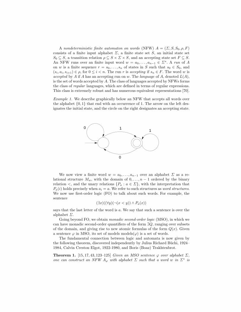
A nondeterministic finite automaton on words (NFW) A = (Σ,S, S0, ρ, F )consists of a finite input alphabet Σ, a finite state set S, an initial state setS0 ⊆ S, a transition relation ρ ⊆ S ×Σ × S, and an accepting state set F ⊆ S.An NFW runs over an finite input word w = a0, . . . , an−1 ∈ Σ∗. A run of Aon w is a finite sequence r = s0, . . . , sn of states in S such that s0 ∈ S0, and(si, ai, si+1) ∈ ρ, for 0 ≤ i < n. The run r is accepting if sn ∈ F . The word w isaccepted by A if A has an accepting run on w. The language of A, denoted L(A),is the set of words accepted byA. The class of languages accepted by NFWs formsthe class of regular languages, which are defined in terms of regular expressions.This class is extremely robust and has numerous equivalent representations [70].

Example 1. We describe graphically below an NFW that accepts all words overthe alphabet {0, 1} that end with an occurrence of 1. The arrow on the left des-ignates the initial state, and the circle on the right designates an accepting state.

0

11

0

We now view a finite word w = a0, . . . , an−1 over an alphabet Σ as a re-lational structure Mw, with the domain of 0, . . . , n − 1 ordered by the binaryrelation <, and the unary relations {Pa : a ∈ Σ}, with the interpretation thatPa(i) holds precisely when ai = a. We refer to such structures as word structures.We now use first-order logic (FO) to talk about such words. For example, thesentence

(∃x)((∀y)(¬(x < y)) ∧ Pa(x))

says that the last letter of the word is a. We say that such a sentence is over thealphabet Σ.

Going beyond FO, we obtain monadic second-order logic (MSO), in which wecan have monadic second-order quantifiers of the form ∃Q, ranging over subsetsof the domain, and giving rise to new atomic formulas of the form Q(x). Givena sentence ϕ in MSO, its set of models models(ϕ) is a set of words.

The fundamental connection between logic and automata is now given bythe following theorem, discovered independently by Julius Richard Buchi, 1924–1984, Calvin Creston Elgot, 1922-1980, and Boris (Boaz) Trakhtenbrot.

Theorem 1. [15, 17, 43, 123–125] Given an MSO sentence ϕ over alphabet Σ,one can construct an NFW Aϕ with alphabet Σ such that a word w in Σ∗ is

accepted by Aϕ iff ϕ holds in the word structure Mw. Conversely, given an NFWA with alphabet Σ, one can construct an MSO sentence ϕA over Σ such thatϕA holds in a word structure Mw iff w is accepted by A.

Thus, the class of languages defined by MSO sentences is precisely the class ofregular languages.

To decide whether a sentence ϕ is satisfiable, that is, whether models(ϕ) 6= ∅,we need to check that L(Aϕ) 6= ∅. This turns out to be an easy problem. LetA = (Σ,S, S0, ρ, F ) be an NFW. Construct a directed graph GA = (S,EA),with S as the set of nodes, and EA = {(s, t) : (s, a, t) ∈ ρ for some a ∈ Σ}. Thefollowing lemma is implicit in [15, 17, 43, 123] and more explicit in [107].

Lemma 1. L(A) 6= ∅ iff there are states s0 ∈ S0 and t ∈ F such that in GA

there is a path from s0 to t.

We thus obtain an algorithm for the Satisfiability problem of MSO overword structures: given an MSO sentence ϕ, construct the NFW Aϕ and checkwhether L(A) 6= ∅ by finding a path from an initial state to an accepting state.This approach to satisfiability checking is referred to as the automata-theoreticapproach, since the decision procedure proceeds by first going from logic to au-tomata, and then searching for a path in the constructed automaton.

There was little interest in the 1950s in analyzing the computational complex-ity of the Satisfiability problem. That had to wait until 1974. Define the func-tion exp(k, n) inductively as follows: exp(0, n) = n and exp(k+1, n) = 2exp(k,n).We say that a problem is nonelementary if it can not be solved by an algorithmwhose running time is bounded by exp(k, n) for some fixed k ≥ 0; that is, therunning time cannot be bounded by a tower of exponentials of a fixed height. Itis not too difficult to observe that the construction of the automaton Aϕ in [15,17, 43, 123] involves a blow-up of exp(n, n), where n is the length of the MSOsentence being decided. It was shown in [88, 116] that the Satisfiability prob-lem for MSO is nonelementary. In fact, the problem is already nonelementaryfor FO [116].

1.2 Reasoning about Sequential Circuits

The field of hardware verification seems to have been started in a little known1957 paper by Alonzo Church, 1903–1995, in which he described the use of logicto specify sequential circuits [24]. A sequential circuit is a switching circuit whoseoutput depends not only upon its input, but also on what its input has been inthe past. A sequential circuit is a particular type of finite-state machine, whichbecame a subject of study in mathematical logic and computer science in the1950s.

Formally, a sequential circuit C = (I,O,R, f, g, r0) consists of a finite set I ofBoolean input signals, a finite set O of Boolean output signals, a finite set R ofBoolean sequential elements, a transition function f : 2I × 2R → 2R, an outputfunction g : 2R → 2O, and an initial state r0 ∈ 2R. (We refer to elements of I ∪O∪R as circuit elements, and assume that I, O, and R are disjoint.) Intuitively,

a state of the circuit is a Boolean assignment to the sequential elements. Theinitial state is r0. In a state r ∈ 2R, the Boolean assignment to the output signalsis g(r). When the circuit is in state r ∈ 2R and it reads an input assignmenti ∈ 2I , it changes its state to f(i, r).

A trace over a set V of Boolean variables is an infinite word over the alphabet2V , i.e., an element of (2V )ω . A trace of the sequential circuit C is a trace overI ∪O ∪R that satisfies some conditions. Specifically, a sequence τ = (i0, r0,o0),(i1, r1,o1), . . ., where ij ∈ 2I , oj ∈ 2O, and rj ∈ 2R, is a trace of C if rj+1 =f(ij, rj) and oj = g(rj), for j ≥ 0. Thus, in modern terminology, Church wasfollowing the linear-time approach [82] (see discussion in Section 2.1). The setof traces of C is denoted by traces(C).

We saw earlier how to associate relational structures with words. We cansimilarly associate with an infinite word w = a0, a1, . . . over an alphabet 2V , arelational structure Mw = (IN,≤, V ), with the naturals IN as the domain, orderedby <, and extended by the set V of unary predicates, where j ∈ p, for p ∈ V ,precisely when p holds (i.e., is assigned 1) in ai.

1 We refer to such structures asinfinite word structures. When we refer to the vocabulary of such a structure, werefer explicitly only to V , taking < for granted.

We can now specify traces using First-Order Logic (FO) sentences con-structed from atomic formulas of the form x = y, x < y, and p(x) for p ∈V = I ∪R ∪O.2 For example, the FO sentence

(∀x)(∃y)(x < y ∧ p(y))

says that p holds infinitely often in the trace. In a follow-up paper in 1963[25], Church considered also specifying traces using monadic second-order logic(MSO), where in addition to first-order quantifiers, which range over the ele-ments of IN, we allow also monadic second-order quantifiers, ranging over subsetsof IN, and atomic formulas of the form Q(x), where Q is a monadic predicatevariable. (This logic is also called S1S, the “second-order theory of one successorfunction”.) For example, the MSO sentence,

(∃P )(∀x)(∀y)((((P (x) ∧ y = x+ 1) → (¬P (y)))∧(((¬P (x)) ∧ y = x+ 1) → P (y)))∧(x = 0 → P (x)) ∧ (P (x) → q(x))),

where x = 0 is an abbrevaition for (¬(∃z)(z < x)) and y = x+ 1 is an abbrevia-tion for (y > x∧¬(∃z)(x < z ∧ z < y)), says that q holds at every even point onthe trace. In effect, Church was proposing to use classical logic (FO or MSO) asa logic of time, by focusing on infinite word structures. The set of infinite modelsof an FO or MSO sentence ϕ is denoted by modelsω(ϕ).

Church posed two problems related to sequential circuits [24]:

– The Decision problem: Given circuit C and a sentence ϕ, does ϕ hold inall traces of C? That is, does traces(C) ⊆ models(ϕ) hold?

1 We overload notation here and treat p as both a Boolean variable and a predicate.2 We overload notation here and treat p as both a circuit element and a predicate

symbol.

– The Synthesis problem: Given sets I and O of input and output signals,and a sentence ϕ over the vocabulary I∪O, construct, if possible, a sequentialcircuit C with input signals I and output signals O such that ϕ holds in alltraces of C. That is, construct C such that traces(C) ⊆ models(ϕ) holds.

In modern terminology, Church’s Decision problem is the model-checking

problem in the linear-time approach (see Section 2.2). This problem did not re-ceive much attention after [24, 25], until the introduction of model checking inthe early 1980s. In contrast, the Synthesis problem has remained a subject ofongoing research; see [18, 76, 78, 106, 122]. One reason that the Decision prob-lem did not remain a subject of study, is the easy observation in [25] that theDecision problem can be reduced to the validity problem in the underlyinglogic (FO or MSO). Given a sequential circuit C, we can easily generate anFO sentence αC that holds in precisely all structures associated with traces ofC. Intuitively, the sentence αC simply has to encode the transition and outputfunctions of C, which are Boolean functions. Then ϕ holds in all traces of Cprecisely when αC → ϕ holds in all word structures (of the appropriate vocab-ulary). Thus, to solve the Decision problem we need to solve the Validity

problem over word structures. As we see next, this problem was solved in 1962.

1.3 Reasoning about Infinite Words

Church’s Decision problem was essentially solved in 1962 by Buchi who showedthat the Validity problem over infinite word structures is decidable [16]. Ac-tually, Buchi showed the decidability of the dual problem, which is the Sat-

isfiability problem for MSO over infinite word structures. Buchi’s approachconsisted of extending the automata-theoretic approach, see Theorem 1, whichwas introduced a few years earlier for word structures, to infinite word struc-tures. To that end, Buchi extended automata theory to automata on infinitewords.

A nondeterministic Buchi automaton on words (NBW) A = (Σ,S, S0, ρ, F )consists of a finite input alphabet Σ, a finite state set S, an initial state setS0 ⊆ S, a transition relation ρ ⊆ S ×Σ × S, and an accepting state set F ⊆ S.An NBW runs over an infinite input word w = a0, a1, . . . ∈ Σω. A run of A onw is an infinite sequence r = s0, s1, . . . of states in S such that s0 ∈ S0, and(si, ai, si+1) ∈ ρ, for i ≥ 0. The run r is accepting if F is visited by r infinitelyoften; that is, si ∈ F for infinitely many i’s. The word w is accepted by A if A hasan accepting run on w. The infinitary language of A, denoted Lω(A), is the setof infinite words accepted by A. The class of languages accepted by NBWs formsthe class of ω-regular languages, which are defined in terms of regular expressionsaugmented with the ω-power operator (eω denotes an infinitary iteration of e)[16].

Example 2. We describe graphically an NBW that accepts all words over thealphabet {0, 1} that contain infinitely many occurrences of 1. The arrow on theleft designates the initial state, and the circle on the right designates an accept-ing state. Note that this NBW looks exactly like the NFW in Example 1. The

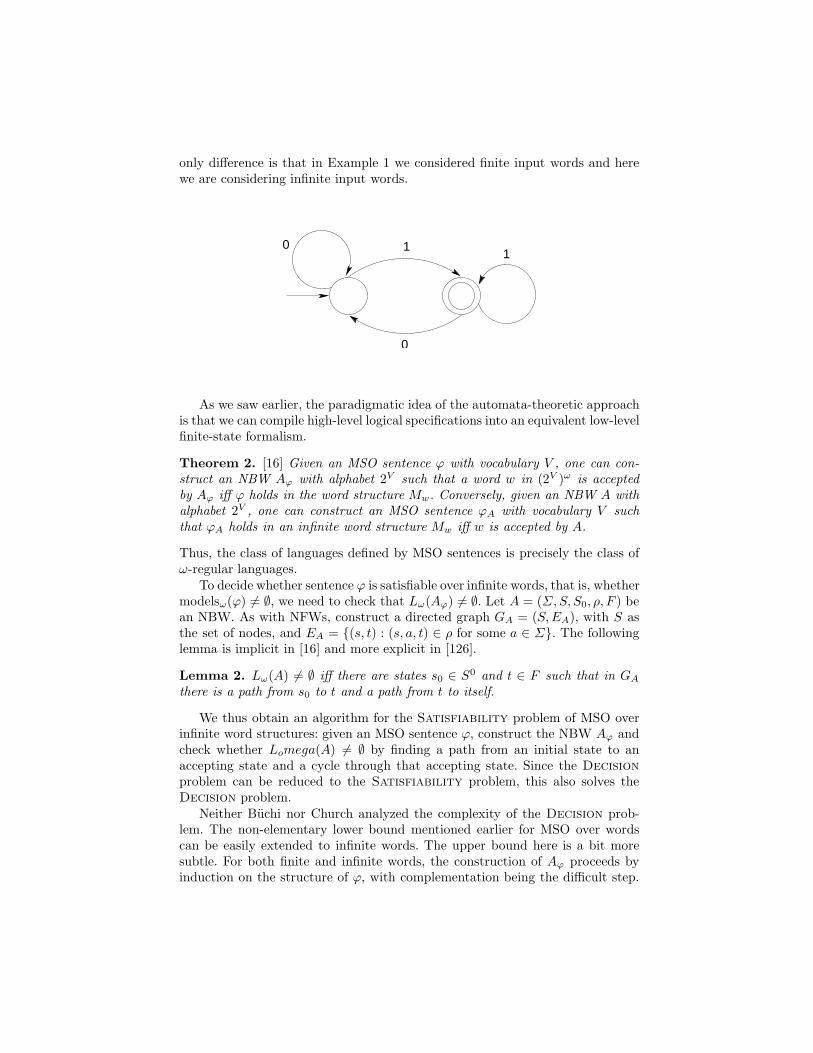
only difference is that in Example 1 we considered finite input words and herewe are considering infinite input words.

0

11

0

As we saw earlier, the paradigmatic idea of the automata-theoretic approachis that we can compile high-level logical specifications into an equivalent low-levelfinite-state formalism.

Theorem 2. [16] Given an MSO sentence ϕ with vocabulary V , one can con-struct an NBW Aϕ with alphabet 2V such that a word w in (2V )ω is acceptedby Aϕ iff ϕ holds in the word structure Mw. Conversely, given an NBW A withalphabet 2V , one can construct an MSO sentence ϕA with vocabulary V suchthat ϕA holds in an infinite word structure Mw iff w is accepted by A.

Thus, the class of languages defined by MSO sentences is precisely the class ofω-regular languages.

To decide whether sentence ϕ is satisfiable over infinite words, that is, whethermodelsω(ϕ) 6= ∅, we need to check that Lω(Aϕ) 6= ∅. Let A = (Σ,S, S0, ρ, F ) bean NBW. As with NFWs, construct a directed graph GA = (S,EA), with S asthe set of nodes, and EA = {(s, t) : (s, a, t) ∈ ρ for some a ∈ Σ}. The followinglemma is implicit in [16] and more explicit in [126].

Lemma 2. Lω(A) 6= ∅ iff there are states s0 ∈ S0 and t ∈ F such that in GA

there is a path from s0 to t and a path from t to itself.

We thus obtain an algorithm for the Satisfiability problem of MSO overinfinite word structures: given an MSO sentence ϕ, construct the NBW Aϕ andcheck whether Lomega(A) 6= ∅ by finding a path from an initial state to anaccepting state and a cycle through that accepting state. Since the Decision

problem can be reduced to the Satisfiability problem, this also solves theDecision problem.

Neither Buchi nor Church analyzed the complexity of the Decision prob-lem. The non-elementary lower bound mentioned earlier for MSO over wordscan be easily extended to infinite words. The upper bound here is a bit moresubtle. For both finite and infinite words, the construction of Aϕ proceeds byinduction on the structure of ϕ, with complementation being the difficult step.

For NFW, complementation uses the subset construction, which involves a blow-up of 2n [107, 109]. Complementation for NBW is significantly more involved,see [127]. The blow-up of complementation is 2Θ(n log n), but there is still a gapbetween the known upper and lower bounds. At any rate, this yields a blow-upof exp(n, n logn) for the translation from MSO to NBW.

2 Thread II: Temporal Logic

2.1 From Aristotle to Kamp

The history of time in logic goes back to ancient times.3 Aristotle ponderedhow to interpret sentences such as “Tomorrow there will be a sea fight,” or“Tomorrow there will not be a sea fight.” Medieval philosophers also ponderedthe issue of time.4 By the Renaissance period, philosophical interest in the logicof time seems to have waned. There were some stirrings of interest in the 19thcentury, by Boole and Peirce. Peirce wrote:

“Time has usually been considered by logicians to be what is called‘extra-logical’ matter. I have never shared this opinion. But I have thoughtthat logic had not yet reached the state of development at which the in-troduction of temporal modifications of its forms would not result ingreat confusion; and I am much of that way of thinking yet.”

There were also some stirrings of interest in the first half of the 20th century,but the birth of modern temporal logic is unquestionably credited to ArthurNorman Prior, 1914-1969. Prior was a philosopher, who was interested in theo-logical and ethical issues. His own religious path was somewhat convoluted; hewas born a Methodist, converted to Presbytarianism, became an atheist, andended up an agnostic. In 1949, he published a book titled “Logic and The Basisof Ethics”. He was particularly interested in the conflict between the assumptionof free will (“the future is to some extent, even if it is only a very small extent,something we can make for ourselves”), foredestination (“of what will be, it hasnow been the case that it will be”), and foreknowledge (“there is a deity whoinfallibly knows the entire future”). He was also interested in modal logic [103].

3 For a detailed history of temporal logic from ancient times to the modern period,see [92].

4 For example, William of Ockham, 1288–1348, wrote (rather obscurely for the modernreader): “Wherefore the difference between present tense propositions and past andfuture tense propositions is that the predicate in a present tense proposition standsin the same way as the subject, unless something added to it stops this; but in a pasttense and a future tense proposition it varies, for the predicate does not merely standfor those things concerning which it is truly predicated in the past and future tensepropositions, because in order for such a proposition to be true, it is not sufficientthat that thing of which the predicate is truly predicated (whether by a verb in thepresent tense or in the future tense) is that which the subject denotes, although it isrequired that the very same predicate is truly predicated of that which the subjectdenotes, by means of what is asserted by such a proposition.”

This confluence of interests led Prior to the development of temporal logic. 5 Hiswife, Mary Prior, recalled after his death:

“I remember his waking me one night [in 1953], coming and sitting onmy bed, . . ., and saying he thought one could make a formalised tenselogic.”

Prior lectured on his new work when he was the John Locke Lecturer at theUniversity of Oxford in 1955–6, and published his book “Time and Modality” in1957 [101].6 In this book, he presented a temporal logic that is propositional logicextended with two temporal connectives, F and P , corresponding to “sometimein the future” and “sometime in the past”. A crucial feature of this logic is thatit has an implicit notion of “now”, which is treated as an indexical, that is, itdepends on the context of utterance for its meaning. Both future and past aredefined with respect to this implicit “now”.

It is interesting to note that the linear vs. branching time dichotomy, whichhas been a subject of some controversy in the computer science literature since1980 (see [132]), has been present from the very beginning of temporal-logicdevelopment. In Prior’s early work on temporal logic, he assumed that time waslinear. In 1958, he received a letter from Saul Kripke,7 who wrote

“In an indetermined system, we perhaps should not regard time as alinear series, as you have done. Given the present moment, there areseveral possibilities for what the next moment may be like – and for eachpossible next moment, there are several possibilities for the moment afterthat. Thus the situation takes the form, not of a linear sequence, but ofa ‘tree’.”

Prior immediately saw the merit of Kripke’s suggestion: “the determinist seestime as a line, and the indeterminist sees times as a system of forking paths.” Hewent on to develop two theories of branching time, which he called “Ockhamist”and “Peircean”. (Prior did not use path quantifiers; those were introduced later,in the 1980s. See Section 3.2.)

While the introduction of branching time seems quite reasonable in the con-text of trying to formalize free will, it is far from being simple philosophically.Prior argued that the nature of the course of time is branching, while the natureof a course of events is linear [102]. In contrast, it was argued in [91] that the

5 An earlier term was tense logic; the term temporal logic was introduced in [91]. Thetechnical distinction between the two terms seems fuzzy.

6 Due to the arcane infix notation of the time, the book may not be too ac-cessible to modern readers, who may have difficulties parsing formulas such asCKMpMqAMKpMqMKqMp.

7 Kripke was a high-school student, not quite 18, in Omaha, Nebraska. Kripke’s in-terest in modal logic was inspired by a paper by Prior on this subject [104]. Priorturned out to be the referee of Kripke’s first paper [75].

nature of time is linear, but the nature of the course of events is branching: “Wehave ‘branching in time,’ not ‘branching of time’.”8

During the 1960s, the development of temporal logic continued through boththe linear-time approach and the branching-time approach. There was little con-nection, however, between research on temporal logic and research on classicallogics, as described in Section 1. That changed in 1968, when Johan AnthonyWillem (Hans) Kamp tied together the two threads in his doctoral dissertation.

Theorem 3. [71] Linear temporal logic with past and binary temporal connec-tives (“strict until” and “strict since”) has precisely the expressive power of FOover the ordered naturals (with monadic vocabularies).

It should be noted that Kamp’s Theorem is actually more general and assertsexpressive equivalence of FO and temporal logic over all “Dedekind-closed or-ders”. The introduction of binary temporal connectives by Kamp was necessaryfor reaching the expressive power of FO; unary linear temporal logic, which hasonly unary temporal connectives, is weaker than FO [51]. The theorem refersto FO formulas with one free variable, which are satisfied at an element of astructure, analogously to temporal logic formulas, which are satisfied at a pointof time.

It should be noted that one direction of Kamp’s Theorem, the translationfrom temporal logic to FO, is quite straightforward; the hard direction is thetranslation from FO to temporal logic. Both directions are algorithmically ef-fective; translating from temporal logic to FO involves a linear blowup, buttranslation in the other direction involves a nonelementary blowup.

If we focus on FO sentences rather than FO formulas, then they define setsof traces (a sentence ϕ defines models(ϕ)). A characterization of of the expres-siveness of FO sentences over the naturals, in terms of their ability to define setsof traces, was obtained in 1979.

Theorem 4. [121] FO sentences over naturals have the expressive power of ∗-free ω-regular expressions.

Recall that MSO defines the class of ω-regular languages. It was already shownin [44] that FO over the naturals is weaker expressively than MSO over thenaturals. Theorem 4 was inspired by an analogous theorem in [87] for finitewords.

2.2 The Temporal Logic of Programs

There were some early observations that temporal logic can be applied to pro-grams. Prior stated: “There are practical gains to be had from this study too, forexample, in the representation of time-delay in computer circuits” [102]. Also, a

8 One is reminded of St. Augustin, who said in his Confessions: “What, then, is time?If no one asks me, I know; but if I wish to explain it to some who should ask me, Ido not know.”

discussion of the application of temporal logic to processes, which are defined as“programmed sequences of states, deterministic or stochastic” appeared in [91].

The “big bang” for the application of temporal logic to program correctnessoccurred with Amir Pnueli’s 1977 paper [94]. In this paper, Pnueli, inspiredby [91], advocated using future linear temporal logic (LTL) as a logic for thespecification of non-terminating programs; see overview in [59].

LTL is a temporal logic with two temporal connectives, “next” and “until”.9

In LTL, formulas are constructed from a set Prop of atomic propositions us-ing the usual Boolean connectives as well as the unary temporal connective X(“next”), and the binary temporal connective U (“until”). Additional unary tem-poral connectives F (“eventually”), and G (“always”) can be defined in termsof U . Note that all temporal connectives refer to the future here, in contrast toKamp’s “strict since” operator, which refers to the past. Thus, LTL is a futuretemporal logic. For extensions with past temporal connectives, see [84, 85, 129].

LTL is interpreted over traces over the set Prop of atomic propositions. Fora trace τ and a point i ∈ IN, the notation τ, i |= ϕ indicates that the formula ϕholds at the point i of the trace τ . Thus, the point i is the implicit “now” withrespect to which the formula is interpreted. We have that

– τ, i |= p if p holds at τ(i),– τ, i |= Xϕ if τ, i+ 1 |= ϕ, and– τ, i |= ϕUψ if for some j ≥ i, we have τ, j |= ψ and for all k, i ≤ k < j, we

have τ, k |= ϕ.

The temporal connectives F and G can be defined in terms of the temporalconnective U ; Fϕ is defined as true Uϕ, and Gϕ is defined as ¬F¬ϕ. We saythat τ satisfies a formula ϕ, denoted τ |= ϕ, iff τ, 0 |= ϕ. We denote by models(ϕ)the set of traces satisfying ϕ.

As an example, the LTL formula G(request → F grant), which refers tothe atomic propositions request and grant, is true in a trace precisely whenevery state in the trace in which request holds is followed by some state in the(non-strict) future in which grant holds. Also, the LTL formula G(request →(request U grant)) is true in a trace precisely if, whenever request holds in astate of the trace, it holds until a state in which grant holds is reached.

The focus on satisfaction at 0, called initial semantics, is motivated by thedesire to specify computations at their starting point. It enables an alternativeversion of Kamp’s Theorem, which does not require past temporal connectives,but focuses on initial semantics.

Theorem 5. [56] LTL has precisely the expressive power of FO over the orderednaturals (with monadic vocabularies) with respect to initial semantics.

As we saw earlier, FO has the expressive power of star-free ω-regular expres-sions over the naturals. Thus, LTL has the expressive power of star-free ω-regular

9 Unlike Kamp’s “strict until” (“p strict until q” requires q to hold in the strict future),Pnueli’s “until” is not strict (“p until q” can be satisfied by q holding now), whichis why the “next” connective is required.

expressions (see [96]), and is strictly weaker than MSO. An interesting outcomeof the above theorem is that it lead to the following assertion regarding LTL[89]: “The corollary due to Meyer – I have to get in my controversial remark – isthat that [Theorem 5] makes it theoretically uninteresting.” Developments since1980 have proven this assertion to be overly pessimistic on the merits of LTL.

Pnueli also discussed the analog of Church’s Decision problem: given afinite-state program P and an LTL formula ϕ, decide if ϕ holds in all tracesof P . Just like Church, Pnueli observed that this problem can be solved byreduction to MSO. Rather than focus on sequential circuits, Pnueli focused onprograms, modeled as (labeled) transition systems [72]. A transition systemM =(W,W0, R, V ) consists of a set W of states that the system can be in, a setW0 ⊆ W of initial states, a transition relation R ⊆ W 2 that indicates theallowable state transitions of the system, and an assignment V : W → 2Prop oftruth values to the atomic propositions in each state of the system. (A transitionsystem is essentially a Kripke structure [10].) A path in M that starts at u isa possible infinite behavior of the system starting at u, i.e., it is an infinitesequence u0, u1 . . . of states in W such that u0 = u, and (ui, ui+1) ∈ R for alli ≥ 0. The sequence V (u0), V (u1) . . . is a trace of M that starts at u. It is thesequence of truth assignments visited by the path. The language of M , denotedL(M), consists of all traces of M that start at a state in W0. Note that L(M)is a language of infinite words over the alphabet 2Prop. The language L(M) canbe viewed as an abstract description of the system M , describing all possibletraces. We say that M satisfies an LTL formula ϕ if all traces in L(M) satisfy ϕ,that is, if L(M) ⊆ models(ϕ). When W is finite, we have a finite-state system,and can apply algorithmic techniques.

What about the complexity of LTL reasoning? Recall from Section 1 thatsatisfiability of FO over trace structures is nonelementary. In contrast, it wasshown in [61, 62, 111–113,138, 139] that LTL Satisfiability is elementary; infact, it is PSPACE-complete. It was also shown that the Decision problem forLTL with respect to finite transition systems is PSPACE-complete [111–113].The basic technique for proving these elementary upper bounds is the tableautechnique, which was adapted from dynamic logics [99] (see Section 3.1). Thus,even though FO and LTL are expressively equivalent, they have dramaticallydifferent computational properties, as LTL reasoning is in PSPACE, while FOreasoning is nonelementary.

The second “big bang” in the application of temporal logic to program cor-rectness was the introduction of model checking by Edmund Melson Clarke andErnest Allen Emerson [28] and by Jean-Pierre Queille and Joseph Sifakis [105].The two papers used two different branching-time logics. Clarke and Emersonused CTL (inspired by the branching-time logic UB of [9]), which extends LTLwith existential and universal path quantifiers E and A. Queille and Sifakis useda logic introduced by Leslie Lamport [82], which extends propositional logic withthe temporal connectives POT (which corresponds to the CTL operator EF )and INEV (which corresponds to the CTL operator AF ). The focus in bothpapers was on model checking, which is essentially what Church called the De-

cision problem: does a given finite-state program, viewed as a finite transitionsystem, satisfy its given temporal specification. In particular, Clarke and Emer-son showed that model checking transition systems of size m with respect toformulas of size n can be done in time polynomial in m and n. This was refinedlater to O(mn) (even in the presence of fairness constraints, which restrict at-tention to certain infinite paths in the underlying transition system) [29, 30]. Wedrop the term “Decision problem” from now on, and replace it with the term“Model-Checking problem”.10

It should be noted that the linear complexity of model checking refers to thesize of the transition system, rather than the size of the program that gave rise tothat system. For sequential circuits, transition-system size is essentially exponen-tial in the size of the description of the circuit (say, in some Hardware DescriptionLanguage). This is referred to as the “state-explosion problem” [31]. In spite ofthe state-explosion problem, in the first few years after the publication of thefirst model-checking papers in 1981-2, Clarke and his students demonstrated thatmodel checking is a highly successful technique for automated program verifica-tion [13, 33]. By the late 1980s, automated verification had become a recognizedresearch area. Also by the late 1980s, symbolic model checking was developed[19, 20], and the SMV tool, developed at CMU by Kenneth Laughlin McMillan[86], was starting to have an industrial impact. See [27] for more details.

The detailed complexity analysis in [29] inspired a similar detailed analysis oflinear time model checking. It was shown in [83] that model checking transitionsystems of size m with respect to LTL formulas of size n can be done in timem2O(n). (This again was shown using a tableau-based technique.) While thebound here is exponential in n, the argument was that n is typically rathersmall, and therefore an exponential bound is acceptable.

2.3 Back to Automata

Since LTL can be translated to FO, and FO can be translated to NBW, it isclear that LTL can be translated to NBW. Going through FO, however, wouldincur, in general, a nonelementary blowup. In 1983, Pierre Wolper, AravindaPrasad Sistla, and I showed that this nonelementary blowup can be avoided.

Theorem 6. [136, 140] Given an LTL formula ϕ of size n, one can construct anNBW Aϕ of size 2O(n) such that a trace σ satisfies ϕ if and only if σ is acceptedby Aϕ.

It now follows that we can obtain a PSPACE algorithm for LTL Satisfia-

bility: given an LTL formula ϕ, we construct Aϕ and check that Aϕ 6= ∅ usingthe graph-theoretic approach described earlier. We can avoid using exponentialspace, by constructing the automaton on the fly [136, 140].

10 The model-checking problem is analogous to database query evaluation, where wecheck the truth of a logical formula, representing a query, with respect to a database,viewed as a finite relational structure. Interestingly, the study of the complexity ofdatabase query evaluation started about the same time as that of model checking[128].

What about model checking? We know that a transition system M satisfiesan LTL formula ϕ if L(M) ⊆ models(ϕ). It was then observed in [135] that thefollowing are equivalent:

– M satisfies ϕ– L(M) ⊆ models(ϕ)– L(M) ⊆ L(Aϕ)– L(M) ∩ ((2Prop)ω − L(Aϕ)) = ∅– L(M) ∩ L(A¬ϕ) = ∅– L(M ×A¬ϕ) = ∅

Thus, rather than complementing Aϕ using an exponential complementationconstruction [16, 77, 115], we complement the LTL property using logical nega-tion. It is easy to see that we can now get the same bound as in [83]: modelchecking programs of size m with respect to LTL formulas of size n can bedone in time m2O(n). Thus, the optimal bounds for LTL satisfiability and modelchecking can be obtained without resorting to ad-hoc tableau-based techniques;the key is the exponential translation of LTL to NBW.

One may wonder whether this theory is practical. Reduction to practice tookover a decade of further research, which saw the development of

– an optimized search algorithm for explicit-state model checking [36, 37],– a symbolic, BDD-based11 algorithm for NBW nonemptiness [19, 20, 49],– symbolic algorithms for LTL to NBW translation [19, 20, 32], and– an optimized explicit algorithm for LTL to NBW translation [58].

By 1995, there were two model-checking tools that implemented LTL modelchecking via the automata-theoretic approach: Spin [69] is an explicit-state LTLmodel checker, and Cadence’s SMV is a symbolic LTL model checker.12 See [133]for a description of algorithmic developments since the mid 1990s. Additionaltools today are VIS [12], NuSMV [26], and SPOT [38].

It should be noted that Robert Kurshan developed the automata-theoreticapproach independently, also going back to the 1980s [1, 2, 79]. In his approach(as also in [108, 140]), one uses automata to represent both the system and itsspecification [80].13 The first implementation of COSPAN, a model-checking toolthat is based on this approach [63], also goes back to the 1980s; see [81].

2.4 Enhancing Expressiveness

Can the development of LTL model checking [83, 135] be viewed as a satisfactorysolution to Church’s Decision problem? Almost, but not quite, since, as we

11 To be precise, one should use the acronym ROBDD, for Reduced Ordered BinaryDecision Diagrams [14].

12 Cadence’s SMV is also a CTL model checker. Seewww.cadence.com/webforms/cbl\_software/index.aspx.

13 The connection to automata is somewhat difficult to discern in the early papers [1,2].

observed earlier, LTL is not as expressive as MSO, which means that LTL isexpressively weaker than NBW. Why do we need the expressive power of NBWs?First, note that once we add fairness to transitions systems (sse [29, 30]), theycan be viewed as variants of NBWs. Second, there are good reasons to expect thespecification language to be as expressive as the underlying model of programs[95]. Thus, achieving the expressive power of NBWs, which we refer to as ω-regularity, is a desirable goal. This motivated efforts since the early 1980s toextend LTL.

The first attempt along this line was made by Wolper [138, 139], who de-fined ETL (for Extended Temporal Logic), which is LTL extended with grammaroperators. He showed that ETL is more expressive than LTL, while its Satis-

fiability problem can still be solved in exponential time (and even PSPACE[111–113]). Then, Sistla, Wolper and I showed how to extend LTL with automataconnectives, reaching ω-regularity, without losing the PSPACE upper bound forthe Satisfiability problem [136, 140]. Actually, three syntactical variations,denoted ETLf , ETLl, and ETLr were shown to be expressively equivalent andhave these properties [136, 140].

Two other ways to achieve ω-regularity were discovered in the 1980s. Thefirst is to enhance LTL with monadic second-order quantifiers as in MSO, whichyields a logic, QPTL, with a nonelementary Satisfiability problem [114, 115].The second is to enhance LTL with least and greatest fixpoints [6, 130], whichyields a logic, µLTL, that achieves ω-regularity, and has a PSPACE upper boundon its Satisfiability and Model-Checking problems [130]. For example, the(not too readable) formula

(νP )(µQ)(P ∧X(p ∨Q)),

where ν and µ denote greatest and least fixpoint operators, respectively, is equiv-alent to the LTL formula GFp, which says that p holds infinitely often.

3 Thread III: Dynamic and Branching-Time Logics

3.1 Dynamic Logics

In 1976, a year before Pnueli proposed using LTL to specify programs, VaughanRonald Pratt proposed using dynamic logic, an extension of modal logic, tospecify programs [97].14 In modal logic 2ϕ means that ϕ holds in all worlds thatare possible with respect to the current world [10]. Thus, 2ϕ can be taken tomean that ϕ holds after an execution of a program step, taking the transitionrelation of the program to be the possibility relation of a Kripke structure. Prattproposed the addition of dynamic modalities [e]ϕ, where e is a program, whichasserts that ϕ holds in all states reachable by an execution of the program e.Dynamic logic can then be viewed as an extension of Hoare logic, since ψ → [e]ϕcorresponds to the Hoare triple {ψ}e{ϕ} (see [3]). See [65] for an extensivecoverage of dynamic logic.

14 See discussion of precursor and related developments, such as [21, 34, 50, 110], in [65].

In 1977, a propositional version of Pratt’s dynamic logic, called PDL, was pro-posed, in which programs are regular expressions over atomic programs [52, 53].It was shown there that the Satisfiability problem for PDL is in NEXPTIMEand EXPTIME-hard. Pratt then proved an EXPTIME upper bound, adaptingtableau techniques from modal logic [98, 99]. (We saw earlier that Wolper thenadapted these techniques to linear-time logic.)

Pratt’s dynamic logic was designed for terminating programs, while Pnueliwas interested in nonterminating programs. This motivated various extensions ofdynamic logic to nonterminating programs [68, 118, 117, 119]. Nevertheless, theselogics are much less natural for the specification of ongoing behavior than tem-poral logic. They inspired, however, the introduction of the (modal) µ-calculusby Dexter Kozen [73, 74]. The µ-calculus is an extension of modal logic with leastand greatest fixpoints. It subsumes expressively essentially all dynamic and tem-poral logics [11]. Kozen’s paper was inspired by previous papers that showed theusefulness of fixpoints in characterizing correctness properties of programs [45,93] (see also [100]). In turn, the µ-calculus inspired the introduction of µLTL,mentioned earlier. The µ-calculus also played an important role in the develop-ment of symbolic model checking [19, 20, 49].

3.2 Branching-Time Logics

Dynamic logic provided a branching-time approach to reasoning about programs,in contrast to Pnueli’s linear-time approach. Lamport was the first to study thedichotomy between linear and branching time in the context of program cor-rectness [82]. This was followed by the introduction of the branching-time logicUB, which extends unary LTL (LTL without the temporal connective “until” )with the existential and universal path quantifiers, E and A [9]. Path quantifiersenable us to quantify over different future behavior of the system. By adaptingPratt’s tableau-based method for PDL to UB, it was shown that its Satis-

fiability problem is in EXPTIME [9]. Clarke and Emerson then added thetemporal conncetive “until” to UB and obtained CTL [28]. (They did not focuson the Satisfiability problem for CTL, but, as we saw earlier, on its Model-

Checking problem; the Satisfiability problem was shown later to be solvablein EXPTIME [47].) Finally, it was shown that LTL and CTL have incomparableexpressive power, leading to the introduction of the branching-time logic CTL∗,which unifies LTL and CTL [46, 48].

The key feature of branching-time logics in the 1980s was the introductionof explicit path quantifiers in [9]. This was an idea that was not discovered byPrior and his followers in the 1960s and 1970s. Most likely, Prior would havefound CTL∗ satisfactory for his philosophical applications and would have seenno need to introduce the “Ockhamist” and “Peircean” approaches.

3.3 Combining Dynamic and Temporal Logics

By the early 1980s it became clear that temporal logics and dynamic logicsprovide two distinct perspectives for specifying programs: the first is state based,

while the second is action based. Various efforts have been made to combine thetwo approaches. These include the introduction of Process Logic [64] (branchingtime), Yet Another Process Logic [134] (branching time), Regular Process Logic[67] (linear time), Dynamic LTL [60] (linear time), and RCTL [8] (branchingtime), which ultimately evolved into Sugar [7]. RCTL/Sugar is unique amongthese logics in that it did not attempt to borrow the action-based part of dynamiclogic. It is a state-based branching-time logic with no notion of actions. Rather,what it borrowed from dynamic logic was the use of regular-expression-baseddynamic modalities. Unlike dynamic logic, which uses regular expressions overprogram statements, RCTL/Sugar uses regular expressions over state predicates,analogously to the automata of ETL [136, 140], which run over sequences offormulas.

4 Thread IV: From LTL to ForSpec and PSL

In the late 1990s and early 2000s, model checking was having an increasingindustrial impact. That led to the development of two industrial temporal logicsbased on LTL: ForSpec, developed by Intel, and PSL, developed by an industrialstandards committee.

4.1 From LTL to ForSpec

Intel’s involvement with model checking started in 1990, when Kurshan, spend-ing a sabbatical year in Israel, conducted a successful feasibility study at theIntel Design Center (IDC) in Haifa, using COSPAN, which at that point wasa prototype tool; see [81]. In 1992, IDC started a pilot project using SMV. By1995, model checking was used by several design projects at Intel, using an inter-nally developed model checker based on SMV. Intel users have found CTL to belacking in expressive power and the Design Technology group at Intel developedits own specification language, FSL. The FSL language was a linear-time logic,and it was model checked using the automata-theoretic approach, but its designwas rather ad-hoc, and its expressive power was unclear; see [54].

In 1997, Intel’s Design Technology group at IDC embarked on the develop-ment of a second-generation model-checking technology. The goal was to developa model-checking engine from scratch, as well as a new specification language.A BDD-based model checker was released in 1999 [55], and a SAT-based modelchecker was released in 2000 [35].

I got involved in the design of the second-generation specification languagein 1997. That language, ForSpec, was released in 2000 [5]. The first issue to bedecided was whether the language should be linear or branching. This led toan in-depth examination of this issue [132], and the decision was to pursue alinear-time language. An obvious candidate was LTL; we saw that by the mid1990s there were both explicit-state and symbolic model checkers for LTL, sothere was no question of feasibility. I had numerous conversations with Limor Fix,Michael Hadash, Yonit Kesten, and Moshe Sananes on this issue. The conclusion

was that LTL is not expressive enough for industrial usage. In particular, manyproperties that are expressible in FSL are not expressible in LTL. Thus, it turnedout that the theoretical considerations regarding the expressiveness of LTL, i.e.,its lack of ω-regularity, had practical significance. I offered two extensions ofLTL; as we saw earlier both ETL and µLTL achieve ω-regularity and have thesame complexity as LTL. Neither of these proposals was accepted, due to theperceived difficulty of usage of such logics by Intel validation engineers, whotypically have only basic familiarity with automata theory and logic.

These conversations continued in 1998, now with Avner Landver. Avner alsoargued that Intel validation engineers would not be receptive to the automata-based formalism of ETL. Being familiar with RCTL/Sugar and its dynamicmodalities [7, 8], he asked me about regular expressions, and my answer was thatregular expressions are equivalent to automata [70], so the automata of ETLf ,which extends LTL with automata on finite words, can be replaced by regu-lar expressions over state predicates. This lead to the development of RELTL,which is LTL augmented by the dynamic regular modalities of dynamic logic(interpreted linearly, as in ETL). Instead of the dynamic-logic notation [e]ϕ,ForSpec uses the more readable (to engineers) (e triggers ϕ), where e is a regu-lar expression over state predicates (e.g., (p ∨ q)∗, (p ∧ q)), and ϕ is a formula.Semantically, τ, i |= (e triggers ϕ) if, for all j ≥ i, if τ [i, j] (that is, the finiteword τ(i), . . . , τ(j)) “matches” e (in the intuitive formal sense), then τ, j |= ϕ;see [22]. Using the ω-regularity of ETLf , it is now easy to show that RELTLalso achieves ω-regularity [5].

While the addition of dynamic modalities to LTL is sufficient to achieve ω-regularity, we decided to also offer direct support to two specification modesoften used by verification engineers at Intel: clocks and resets. Both clocks andresets are features that are needed to address the fact that modern semiconductordesigns consist of interacting parallel modules. While clocks and resets have asimple underlying intuition, defining their semantics formally is quite nontrivial.ForSpec is essentially RELTL, augmented with features corresponding to clocksand resets, as we now explain.

Today’s semiconductor designs are still dominated by synchronous circuits.In synchronous circuits, clock signals synchronize the sequential logic, providingthe designer with a simple operational model. While the asynchronous approachholds the promise of greater speed (see [23]), designing asynchronous circuits issignificantly harder than designing synchronous circuits. Current design method-ology attempts to strike a compromise between the two approaches by usingmultiple clocks. This results in architectures that are globally asynchronous butlocally synchronous. The temporal-logic literature mostly ignores the issue ofexplicitly supporting clocks. ForSpec supports multiple clocks via the notion ofcurrent clock. Specifically, ForSpec has a construct change on c ϕ, which statesthat the temporal formula ϕ is to be evaluated with respect to the clock c; thatis, the formula ϕ is to be evaluated in the trace defined by the high phases ofthe clock c. The key feature of clocks in ForSpec is that each subformula mayadvance according to a different clock [5].

Another feature of modern designs’ consisting of interacting parallel modulesis the fact that a process running on one module can be reset by a signal comingfrom another module. As noted in [120], reset control has long been a criticalaspect of embedded control design. ForSpec directly supports reset signals. Theformula accept on a ϕ states that the property ϕ should be checked only un-til the arrival of the reset signal a, at which point the check is considered tohave succeeded. In contrast, reject on r ϕ states that the property ϕ shouldbe checked only until the arrival of the reset signal r, at which point the checkis considered to have failed. The key feature of resets in ForSpec is that eachsubformula may be reset (positively or negatively) by a different reset signal; fora longer discussion see [5].

ForSpec is an industrial property-specification language that supports hardware-oriented constructs as well as uniform semantics for formal and dynamic valida-tion, while at the same time it has a well understood expressiveness (ω-regularity)and computational complexity (Satisfiability and Model-Checking prob-lems have the same complexity for ForSpec as for LTL) [5]. The design effortstrove to find an acceptable compromise, with trade-offs clarified by theory, be-tween conflicting demands, such as expressiveness, usability, and implementabil-ity. Clocks and resets, both important to hardware designers, have a clear intu-itive semantics, but formalizing this semantics is nontrivial. The rigorous seman-tics, however, not only enabled mechanical verification of various theorems aboutthe language, but also served as a reference document for the implementors. Theimplementation of model checking for ForSpec followed the automata-theoreticapproach, using alternating automata as advocated in [131] (see [57]).

4.2 From ForSpec to PSL

In 2000, the Electronic Design Automation Association instituted a standardiza-tion body called Accellera.15 Accellera’s mission is to drive worldwide develop-ment and use of standards required by systems, semiconductor and design toolscompanies. Accellera decided that the development of a standard specificationlanguage is a requirement for formal verification to become an industrial reality(see [81]). Since the focus was on specifying properties of designs rather than de-signs themselves, the chosen term was “property specification language” (PSL).The PSL standard committee solicited industrial contributions and received fourlanguage contributions: CBV, from Motorola, ForSpec, from Intel, Temporal e,from Verisity [90], and Sugar, from IBM.

The committee’s discussions were quite fierce.16 Ultimately, it became clearthat while technical considerations play an important role, industrial commit-tees’ decisions are ultimately made for business considerations. In that con-tention, IBM had the upper hand, and Accellera chose Sugar as the base lan-guage for PSL in 2003. At the same time, the technical merits of ForSpec wereaccepted and PSL adopted all the main features of ForSpec. In essence, PSL (the

15 See http://www.accellera.org/.16 See http://www.eda-stds.org/vfv/.

current version 1.1) is LTL, extended with dynamic modalities (referred to asthe regular layer), clocks, and resets (called aborts). PSL did inherit the syntaxof Sugar, and does include a branching-time extension as an acknowledgment toSugar.17

There was some evolution of PSL with respect to ForSpec. After some debateon the proper way to define resets [4], ForSpec’s approach was essentially ac-cepted after some reformulation [41]. ForSpec’s fundamental approach to clocks,which is semantic, was accepted, but modified in some important details [42].In addition to the dynamic modalities, borrowed from dynamic logic, PSL alsohas weak dynamic modalities [40], which are reminiscent of “looping” modalitiesin dynamic logic [68, 66]. Today PSL 1.1 is an IEEE Standard 1850–2005, andcontinues to be refined by the IEEE P1850 PSL Working Group.18

Practical use of ForSpec and PSL has shown that the regular layer (that is,the dynamic modalities), is highly popular with verification engineers. Anotherstandardized property specification language, called SVA (for SystemVerilog As-sertions), is based, in essence, on that regular layer [137].

5 Contemplation

The evolution of ideas, from Church and Prior to PSL, seems to be an amazingdevelopment. It reminds me of the medieval period, when building a cathedralspanned more than a mason’s lifetime. Many masons spend their whole livesworking on a cathedral, never seeing it to completion. We are fortunate to seethe completion of this particular “cathedral”. Just like the medieval masons,our contributions are often smaller than we’d like to consider them, but evensmall contributions can have a major impact. Unlike the medieval cathedrals,the scientific cathedral has no architect; the construction is driven by a com-plex process, whose outcome is unpredictable. Much that has been discovered isforgotten and has to be rediscovered. It is hard to fathom what our particular“cathedral” will look like in 50 years.

Acknowledgments

I am grateful to E. Clarke, A. Emerson, R. Goldblatt, A. Pnueli, P. Sistla,P. Wolper for helping me trace the many threads of this story, to D. Fisman,C. Eisner, J. Halpern, D. Harel and T. Wilke for their many useful commentson earlier drafts of this paper, and to S. Nain, K. Rozier, and D. Tabakov forproofreading earlier drafts. I’d also like to thank K. Rozier for her help withgraphics.

17 See [39] and language reference manual at http://www.eda.org/vfv/docs/PSL-v1.1.pdf.

18 See http://www.eda.org/ieee-1850/.

References

1. S. Aggarwal and R.P. Kurshan. Automated implementation from formal specifi-cation. In Proc. 4th Int’l Workshop on Protocol Specification, Testing and Veri-fication, pages 127–136. North-Holland, 1984.

2. S. Aggarwal, R.P. Kurshan, and D. Sharma. A language for the specificationand analysis of protocols. In Proc. 3rd Int’l Workshop on Protocol Specification,Testing, and Verification, pages 35–50. North-Holland, 1983.

3. K. Apt and E.R. Olderog. Verification of Sequential and Concurrent Programs.Springer, 2006.

4. R. Armoni, D. Bustan, O. Kupferman, and M.Y. Vardi. Resets vs. aborts inlinear temporal logic. In Proc. 9th Int. Conf. on Tools and Algorithms for theConstruction and Analysis of Systems, volume 2619 of Lecture Notes in ComputerScience, pages 65 – 80. Springer, 2003.

5. R. Armoni, L. Fix, A. Flaisher, R. Gerth, B. Ginsburg, T. Kanza, A. Landver,S. Mador-Haim, E. Singerman, A. Tiemeyer, M.Y. Vardi, and Y. Zbar. TheForSpec temporal logic: A new temporal property-specification logic. In Proc. 8thInt. Conf. on Tools and Algorithms for the Construction and Analysis of Systems,volume 2280 of Lecture Notes in Computer Science, pages 296–211. Springer, 2002.

6. B. Banieqbal and H. Barringer. Temporal logic with fixed points. In B. Banieqbal,H. Barringer, and A. Pnueli, editors, Temporal Logic in Specification, volume 398of Lecture Notes in Computer Science, pages 62–74. Springer, 1987.

7. I. Beer, S. Ben-David, C. Eisner, D. Fisman, A. Gringauze, and Y. Rodeh. Thetemporal logic Sugar. In Proc 13th Int. Conf. on Computer Aided Verification,volume 2102 of Lecture Notes in Computer Science, pages 363–367. Springer,2001.

8. I. Beer, S. Ben-David, and A. Landver. On-the-fly model checking of RCTLformulas. In Proc 10th Int. Conf. on Computer Aided Verification, volume 1427of Lecture Notes in Computer Science, pages 184–194. Springer, 1998.

9. M. Ben-Ari, Z. Manna, and A. Pnueli. The logic of nexttime. In Proc. 8th ACMSymp. on Principles of Programming Languages, pages 164–176, 1981.

10. P. Blackburn, M. de Rijke, and Y. Venema. Modal Logic. Cambridge UniversityPress, 2002.

11. J. Bradfield and C. Stirling. PDL and modal µ-calculus. In P. Blackburn, J. vanBenthem, and F. Wolter, editors, Handbook of Modal Logic. Elsevier, 2006.

12. R.K. Brayton, G.D. Hachtel, A. Sangiovanni-Vincentelli, F. Somenzi, A. Aziz, S.-T. Cheng, S. Edwards, S. Khatri, T. Kukimoto, A. Pardo, S. Qadeer, R.K. Ranjan,S. Sarwary, T.R. Shiple, G. Swamy, and T. Villa. VIS: a system for verificationand synthesis. In Proc 8th Int. Conf. on Computer Aided Verification, volume1102 of Lecture Notes in Computer Science, pages 428–432. Springer, 1996.

13. M.C. Browne, E.M. Clarke, D.L. Dill, and B. Mishra. Automatic verificationof sequential circuits using temporal logic. IEEE Transactions on Computing,C-35:1035–1044, 1986.

14. R.E. Bryant. Graph-based algorithms for Boolean-function manipulation. IEEETransactions on Computing, C-35(8):677–691, 1986.

15. J.R. Buchi. Weak second-order arithmetic and finite automata. Zeit. Math. Logikund Grundl. Math., 6:66–92, 1960.

16. J.R. Buchi. On a decision method in restricted second order arithmetic. In Proc.Int. Congress on Logic, Method, and Philosophy of Science. 1960, pages 1–12.Stanford University Press, 1962.

17. J.R. Buchi, C.C. Elgot, and J.B. Wright. The non-existence of certain algorithmsfor finite automata theory (abstract). Notices Amer. Math. Soc., 5:98, 1958.

18. J.R. Buchi and L.H. Landweber. Solving sequential conditions by finite-statestrategies. Trans. AMS, 138:295–311, 1969.

19. J.R. Burch, E.M. Clarke, K.L. McMillan, D.L. Dill, and L.J. Hwang. Symbolicmodel checking: 1020 states and beyond. In Proc. 5th IEEE Symp. on Logic inComputer Science, pages 428–439, 1990.

20. J.R. Burch, E.M. Clarke, K.L. McMillan, D.L. Dill, and L.J. Hwang. Sym-bolic model checking: 1020 states and beyond. Information and Computation,98(2):142–170, 1992.

21. R.M. Burstall. Program proving as hand simulation with a little induction. In In-formation Processing 74, pages 308–312, Stockholm, Sweden, 1974. InternationalFederation for Information Processing, North-Holland.

22. D. Bustan, A. Flaisher, O. Grumberg, O. Kupferman, and M.Y. Vardi. Regularvacuity. In Proc. 13th Conf. on Correct Hardware Design and Verification Meth-ods, volume 3725 of Lecture Notes in Computer Science, pages 191–206. Springer,2005.

23. S.M. Nowick C.H. van Berkel, M.B. Josephs. Applications of asynchronous cir-cuits. Proceedings of the IEEE, 87(2):223–233, 1999.

24. A. Church. Applicaton of recursive arithmetics to the problem of circuit synthesis.In Summaries of Talks Presented at The Summer Institute for Symbolic Logic,pages 3–50. Communications Research Division, Institute for Defense Analysis,1957.

25. A. Church. Logic, arithmetics, and automata. In Proc. Int. Congress of Mathe-maticians, 1962, pages 23–35. Institut Mittag-Leffler, 1963.

26. A. Cimatti, E.M. Clarke, E. Giunchiglia, F. Giunchiglia, M. Pistore, M. Roveri,R. Sebastiani, and A. Tacchella. Nusmv 2: An opensource tool for symbolic modelchecking. In Proc. 14th Int’l Conf. on Computer Aided Verification, Lecture Notesin Computer Science 2404, pages 359–364. Springer, 2002.

27. E.M. Clarke. The birth of model checking. This Volume, 2007.28. E.M. Clarke and E.A. Emerson. Design and synthesis of synchronization skeletons

using branching time temporal logic. In Proc. Workshop on Logic of Programs,volume 131 of Lecture Notes in Computer Science, pages 52–71. Springer, 1981.

29. E.M. Clarke, E.A. Emerson, and A.P. Sistla. Automatic verification of finite stateconcurrent systems using temporal logic specifications: A practical approach. InProc. 10th ACM Symp. on Principles of Programming Languages, pages 117–126,1983.

30. E.M. Clarke, E.A. Emerson, and A.P. Sistla. Automatic verification of finite-state concurrent systems using temporal logic specifications. ACM Transactionson Programming Languagues and Systems, 8(2):244–263, 1986.

31. E.M. Clarke and O. Grumberg. Avoiding the state explosion problem in temporallogic model-checking algorithms. In Proc. 16th ACM Symp. on Principles ofDistributed Computing, pages 294–303, 1987.

32. E.M. Clarke, O. Grumberg, and K. Hamaguchi. Another look at LTL modelchecking. In Proc 6th Int. Conf. on Computer Aided Verification, Lecture Notesin Computer Science, pages 415 – 427. Springer, 1994.

33. E.M. Clarke and B. Mishra. Hierarchical verification of asynchronous circuitsusing temporal logic. Theoretical Computer Science, 38:269–291, 1985.

34. R.L. Constable. On the theory of programming logics. In Proc. 9th ACM Symp.on Theory of Computing, pages 269–285, 1977.

35. F. Copty, L. Fix, R. Fraer, E. Giunchiglia, G. Kamhi, A. Tacchella, and M.Y.Vardi. Benefits of bounded model checking at an industrial setting. In Proc13th Int. Conf. on Computer Aided Verification, volume 2102 of Lecture Notes inComputer Science, pages 436–453. Springer, 2001.

36. C. Courcoubetis, M.Y. Vardi, P. Wolper, and M. Yannakakis. Memory efficientalgorithms for the verification of temporal properties. In Proc 2nd Int. Conf. onComputer Aided Verification, volume 531 of Lecture Notes in Computer Science,pages 233–242. Springer, 1990.

37. C. Courcoubetis, M.Y. Vardi, P. Wolper, and M. Yannakakis. Memory efficientalgorithms for the verification of temporal properties. Formal Methods in SystemDesign, 1:275–288, 1992.

38. A. Duret-Lutz and Denis Poitrenaud. SPOT: An extensible model checkinglibrary using transition-based generalized buchi automata. In Proc. 12th Int’lWorkshop on Modeling, Analysis, and Simulation of Computer and Telecommu-nication Systems, pages 76–83. IEEE Computer Society, 2004.

39. C. Eisner and D. Fisman. A Practical Introduction to PSL. Springer, 2006.

40. C. Eisner, D. Fisman, and J. Havlicek. A topological characterization of weakness.In Proc. 24th ACM Symp. on Principles of Distributed Computing, pages 1–8,2005.

41. C. Eisner, D. Fisman, J. Havlicek, Y. Lustig, A. McIsaac, and D. Van Camp-enhout. Reasoning with temporal logic on truncated paths. In Proc. 15th Int’lConf. on Computer Aided Verification, volume 2725 of Lecture Notes in ComputerScience, pages 27–39. Springer, 2003.

42. C. Eisner, D. Fisman, J. Havlicek, A. McIsaac, and D. Van Campenhout. Thedefinition of a temporal clock operator. In Proc. 30th Int’l Colloquium on Au-tomata, Languages and Programming, volume 2719 of Lecture Notes in ComputerScience, pages 857–870. Springer, 2003.

43. C. Elgot. Decision problems of finite-automata design and related arithmetics.Trans. Amer. Math. Soc., 98:21–51, 1961.

44. C.C. Elgot and J. Wright. Quantifier elimination in a problem of logical design.Michigan Math. J., 6:65–69, 1959.

45. E.A. Emerson and E.M. Clarke. Characterizing correctness properties of parallelprograms using fixpoints. In Proc. 7th Int. Colloq. on Automata, Languages, andProgramming, pages 169–181, 1980.

46. E.A. Emerson and J.Y. Halpern. “Sometimes” and “not never” revisited: Onbranching versus linear time. In Proc. 10th ACM Symp. on Principles of Pro-gramming Languages, pages 127–140, 1983.

47. E.A. Emerson and J.Y. Halpern. Decision procedures and expressiveness in thetemporal logic of branching time. Journal of Computer and Systems Science,30:1–24, 1985.

48. E.A. Emerson and J.Y. Halpern. Sometimes and not never revisited: On branchingversus linear time. Journal of the ACM, 33(1):151–178, 1986.

49. E.A. Emerson and C.-L. Lei. Efficient model checking in fragments of the propo-sitional µ-calculus. In Proc. 1st IEEE Symp. on Logic in Computer Science, pages267–278, 1986.

50. E. Engeler. Algorithmic properties of structures. Math. Syst. Theory, 1:183–195,1967.

51. K. Etessami, M.Y. Vardi, and T. Wilke. First-order logic with two variables andunary temporal logic. Inf. Comput., 179(2):279–295, 2002.

52. M.J. Fischer and R.E. Ladner. Propositional modal logic of programs (extendedabstract). In Proc. 9th ACM Symp. on Theory of Computing, pages 286–294,1977.

53. M.J. Fischer and R.E. Ladner. Propositional dynamic logic of regular programs.Journal of Computer and Systems Science, 18:194–211, 1979.

54. L. Fix. Fifteen years of formal property verification at Intel. In Proc. 2006Workshop on 25 Years of Model Checking, Lecture Notes in Conmputer Science.Springer, 2007.

55. L. Fix and G. Kamhi. Adaptive variable reordering for symbolic model checking.In Proc. ACM/IEEE Int’l Conf. on Computer Aided Design, pages 359–365, 1998.

56. D. Gabbay, A. Pnueli, S. Shelah, and J. Stavi. On the temporal analysis offairness. In Proc. 7th ACM Symp. on Principles of Programming Languages,pages 163–173, 1980.

57. P. Gastin and D. Oddoux. Fast LTL to Buchi automata translation. In Proc13th Int. Conf. on Computer Aided Verification, volume 2102 of Lecture Notes inComputer Science, pages 53–65. Springer, 2001.

58. R. Gerth, D. Peled, M.Y. Vardi, and P. Wolper. Simple on-the-fly automaticverification of linear temporal logic. In P. Dembiski and M. Sredniawa, editors,Protocol Specification, Testing, and Verification, pages 3–18. Chapman & Hall,1995.

59. R. Goldblatt. Logic of time and computation. Technical report, CSLI LectureNotes, no.7, Stanford University, 1987.

60. T. Hafer and W. Thomas. Computation tree logic CTL? and path quantifiers inthe monadic theory of the binary tree. In Proc. 14th Int. Colloq. on Automata,Languages, and Programming, volume 267 of Lecture Notes in Computer Science,pages 269–279. Springer, 1987.

61. JY. Halpern and J.H. Reif. The propositional dynamic logic of deterministic,well-structured programs (extended abstract). In Proc. 22nd IEEE Symp. onFoundations of Computer Science, pages 322–334, 1981.

62. J.Y. Halpern and J.H. Reif. The propositional dynamic logic of deterministic,well-structured programs. Theor. Comput. Sci., 27:127–165, 1983.

63. R.H. Hardin, Z. Har’el, and R.P. Kurshan. COSPAN. In Proc 8th Int. Conf. onComputer Aided Verification, volume 1102 of Lecture Notes in Computer Science,pages 423–427. Springer, 1996.

64. D. Harel, D. Kozen, and R. Parikh. Process logic: Expressiveness, decidability,completeness. J. Comput. Syst. Sci., 25(2):144–170, 1982.

65. D. Harel, D. Kozen, and J. Tiuryn. Dynamic Logic. MIT Press, 2000.66. D. Harel and D. Peleg. More on looping vs. repeating in dynamic logic. Inf.

Process. Lett., 20(2):87–90, 1985.67. D. Harel and D. Peleg. Process logic with regular formulas. Theoreti. Comp. Sci.,

38(2–3):307–322, 1985.68. D. Harel and R. Sherman. Looping vs. repeating in dynamic logic. Inf. Comput.,

55(1–3):175–192, 1982.69. G.J. Holzmann. The model checker SPIN. IEEE Transactions on Software Engi-

neering, 23(5):279–295, 1997.70. J.E. Hopcroft and J.D. Ullman. Introduction to Automata Theory, Languages,

and Computation. Addison-Wesley, 1979.71. J.A.W. Kamp. Tense Logic and the Theory of Order. PhD thesis, UCLA, 1968.72. R.M. Keller. Formal verification of parallel programs. Communications of the

ACM, 19:371–384, 1976.

73. D. Kozen. Results on the propositional µ-calculus. In Proc. 9th Colloquium onAutomata, Languages and Programming, volume 140 of Lecture Notes in Com-puter Science, pages 348–359. Springer, 1982.

74. D. Kozen. Results on the propositional µ-calculus. Theoretical Computer Science,27:333–354, 1983.

75. S. Kripke. A completeness theorem in modal logic. Journal of Symbolic Logic,24:1–14, 1959.

76. O. Kupferman, N. Piterman, and M.Y. Vardi. Safraless compositional synthesis.In Proc 18th Int. Conf. on Computer Aided Verification, volume 4144 of LectureNotes in Computer Science, pages 31–44. Springer, 2006.

77. O. Kupferman and M.Y. Vardi. Weak alternating automata are not that weak.ACM Transactions on Computational Logic, 2(2):408–429, 2001.

78. O. Kupferman and M.Y. Vardi. Safraless decision procedures. In Proc. 46th IEEESymp. on Foundations of Computer Science, pages 531–540, 2005.

79. R.P. Kurshan. Analysis of discrete event coordination. In J.W. de Bakker, W.P.de Roever, and G. Rozenberg, editors, Proc. REX Workshop on Stepwise Refine-ment of Distributed Systems, Models, Formalisms, and Correctness, volume 430of Lecture Notes in Computer Science, pages 414–453. Springer, 1990.

80. R.P. Kurshan. Computer Aided Verification of Coordinating Processes. PrincetonUniv. Press, 1994.

81. R.P. Kurshan. Verification technology transfer. In Proc. 2006 Workshop on 25Years of Model Checking, Lecture Notes in Conmputer Science. Springer, 2007.

82. L. Lamport. “Sometimes” is sometimes “not never” - on the temporal logic ofprograms. In Proc. 7th ACM Symp. on Principles of Programming Languages,pages 174–185, 1980.

83. O. Lichtenstein and A. Pnueli. Checking that finite state concurrent programssatisfy their linear specification. In Proc. 12th ACM Symp. on Principles ofProgramming Languages, pages 97–107, 1985.

84. O. Lichtenstein, A. Pnueli, and L. Zuck. The glory of the past. In Logics ofPrograms, volume 193 of Lecture Notes in Computer Science, pages 196–218.Springer, 1985.

85. N. Markey. Temporal logic with past is exponentially more succinct. EATCSBulletin, 79:122–128, 2003.

86. K.L. McMillan. Symbolic Model Checking. Kluwer Academic Publishers, 1993.

87. R. McNaughton and S. Papert. Counter-Free Automata. MIT Pres, 1971.

88. A. R. Meyer. Weak monadic second order theory of successor is not elementaryrecursive. In Proc. Logic Colloquium, volume 453 of Lecture Notes in Mathematics,pages 132–154. Springer, 1975.

89. A.R. Meyer. Ten thousand and one logics of programming”. Technical report,MIT, 1980. MIT-LCS-TM-150.

90. M.J. Morley. Semantics of temporal e. In T. F. Melham and F.G. Moller, editors,Banff’99 Higher Order Workshop (Formal Methods in Computation). Universityof Glasgow, Department of Computing Science Technical Report, 1999.

91. A. Urquhart N. Rescher. Temporal Logic. Springer, 1971.

92. P. Øhrstrøm and P.F.V. Hasle. Temporal Logic: from Ancient Times to ArtificialIntelligence. Studies in Linguistics and Philosophy, vol. 57. Kluwer, 1995.

93. D. Park. Finiteness is µ-ineffable. Theoretical Computer Science, 3:173–181, 1976.

94. A. Pnueli. The temporal logic of programs. In Proc. 18th IEEE Symp. on Foun-dations of Computer Science, pages 46–57, 1977.

95. A. Pnueli. Linear and branching structures in the semantics and logics of reactivesystems. In Proc. 12th Int. Colloq. on Automata, Languages, and Programming,volume 194 of Lecture Notes in Computer Science, pages 15–32. Springer, 1985.

96. A. Pnueli and L. Zuck. In and out of temporal logic. In Proc. 8th IEEE Symp.on Logic in Computer Science, pages 124–135, 1993.

97. V.R. Pratt. Semantical considerations on Floyd-Hoare logic. In Proc. 17th IEEESymp. on Foundations of Computer Science, pages 109–121, 1976.

98. V.R. Pratt. A practical decision method for propositional dynamic logic: Prelim-inary report. In Proc. 10th Annual ACM Symposium on Theory of Computing,pages 326–337, 1978.

99. V.R. Pratt. A near-optimal method for reasoning about action. Journal of Com-puter and Systems Science, 20(2):231–254, 1980.

100. V.R. Pratt. A decidable µ-calculus: preliminary report. In Proc. 22nd IEEESymp. on Foundations of Computer Science, pages 421–427, 1981.

101. A. Prior. Time and Modality. Oxford University Press, 1957.102. A. Prior. Past, Present, and Future. Clarendon Press, 1967.103. A.N. Prior. Modality de dicto and modality de re. Theoria, 18:174–180, 1952.104. A.N. Prior. Modality and quantification in s5. J. Symbolic Logic, 21:60–62, 1956.105. J.P. Queille and J. Sifakis. Specification and verification of concurrent systems in

Cesar. In Proc. 9th ACM Symp. on Principles of Programming Languages, volume137 of Lecture Notes in Computer Science, pages 337–351. Springer, 1982.

106. M.O. Rabin. Automata on infinite objects and Church’s problem. Amer. Mathe-matical Society, 1972.

107. M.O. Rabin and D. Scott. Finite automata and their decision problems. IBMJournal of Research and Development, 3:115–125, 1959.

108. K. Sabnani, P. Wolper, and A. Lapone. An algorithmic technique for protocolverification. In Proc. Globecom ’85, 1985.

109. W. Sakoda and M. Sipser. Non-determinism and the size of two-way automata.In Proc. 10th ACM Symp. on Theory of Computing, pages 275–286, 1978.

110. A. Salwicki. Algorithmic logic: a tool for investigations of programs. In R.E. Buttsand J. Hintikka, editors, Logic Foundations of Mathematics and ComputabilityTheory, pages 281–295. Reidel, 1977.

111. A.P. Sistla. Theoretical issues in the design of distributed and concurrent systems.PhD thesis, Harvard University, 1983.

112. A.P. Sistla and E.M. Clarke. The complexity of propositional linear temporallogics. In Proc. 14th Annual ACM Symposium on Theory of Computing, pages159–168, 1982.

113. A.P. Sistla and E.M. Clarke. The complexity of propositional linear temporallogic. Journal of the ACM, 32:733–749, 1985.

114. A.P. Sistla, M.Y. Vardi, and P. Wolper. The complementation problem for Buchiautomata with applications to temporal logic. In Proc. 12th Int. Colloq. on Au-tomata, Languages, and Programming, volume 194, pages 465–474. Springer, 1985.

115. A.P. Sistla, M.Y. Vardi, and P. Wolper. The complementation problem for Buchiautomata with applications to temporal logic. Theoretical Computer Science,49:217–237, 1987.

116. L.J. Stockmeyer. The complexity of decision procedures in Automata Theory andLogic. PhD thesis, MIT, 1974. Project MAC Technical Report TR-133.

117. R.S. Street. Propositional dynamic logic of looping and converse. In Proc. 13thACM Symp. on Theory of Computing, pages 375–383, 1981.

118. R.S. Streett. A propositional dynamic logic for reasoning about program diver-gence. PhD thesis, M.Sc. Thesis, MIT, 1980.

119. R.S. Streett. Propositional dynamic logic of looping and converse. Informationand Control, 54:121–141, 1982.

120. A comparison of reset control methods: Application note 11.http://www.summitmicro.com/tech support/notes/note11.htm, SummitMicroelectronics, Inc., 1999.

121. W. Thomas. Star-free regular sets of ω-sequences. Information and Control,42(2):148–156, 1979.

122. W. Thomas. On the synthesis of strategies in infinite games. In E.W. Mayr andC. Puech, editors, Proc. 12th Symp. on Theoretical Aspects of Computer Science,volume 900 of Lecture Notes in Computer Science, pages 1–13. Springer, 1995.

123. B. Trakhtenbrot. The synthesis of logical nets whose operators are described interms of one-place predicate calculus. Doklady Akad. Nauk SSSR, 118(4):646–649,1958.

124. B. Trakhtenbrot. Certain constructions in the logic of one-place predicates. Dok-lady Akad. Nauk SSSR, 138:320–321, 1961.

125. B.A. Trakhtenbrot. Finite automata and monadic second order logic. SiberianMath. J, 3:101–131, 1962. Russian; English translation in: AMS Transl. 59 (1966),23-55.

126. B.A. Trakhtenbrot and Y.M. Barzdin. Finite Automata. North Holland, 1973.127. M. Y. Vardi. The buchi complementation saga. In Proc. 24th Sympo. on Theo-

retical Aspects of Computer Science, volume 4393 of Lecture Notes in ComputerScience, pages 12–22. Springer, 2007.

128. M.Y. Vardi. The complexity of relational query languages. In Proc. 14th ACMSymp. on Theory of Computing, pages 137–146, 1982.

129. M.Y. Vardi. A temporal fixpoint calculus. In Proc. 15th ACM Symp. on Principlesof Programming Languages, pages 250–259, 1988.

130. M.Y. Vardi. Unified verification theory. In B. Banieqbal, H. Barringer, andA. Pnueli, editors, Proc. Temporal Logic in Specification, volume 398, pages 202–212. Springer, 1989.

131. M.Y. Vardi. Nontraditional applications of automata theory. In Proc. 11th Symp.on Theoretical Aspects of Computer Science, volume 789 of Lecture Notes in Com-puter Science, pages 575–597. Springer, 1994.

132. M.Y. Vardi. Branching vs. linear time: Final showdown. In Proc. 7th Int. Conf.on Tools and Algorithms for the Construction and Analysis of Systems, volume2031 of Lecture Notes in Computer Science, pages 1–22. Springer, 2001.

133. M.Y. Vardi. Automata-theoretic model checking revisited. In Proc. 8th Int.Conf. on Verification, Model Checking, and Abstract Interpretation, volume 4349of Lecture Notes in Computer Science, pages 137–150. Springer, 2007.

134. M.Y. Vardi and P. Wolper. Yet another process logic. In Logics of Programs,volume 164 of Lecture Notes in Computer Science, pages 501–512. Springer, 1984.

135. M.Y. Vardi and P. Wolper. An automata-theoretic approach to automatic pro-gram verification. In Proc. 1st IEEE Symp. on Logic in Computer Science, pages332–344, 1986.

136. M.Y. Vardi and P. Wolper. Reasoning about infinite computations. Informationand Computation, 115(1):1–37, 1994.

137. S. Vijayaraghavan and M. Ramanathan. A Practical Guide for SystemVerilogAssertions. Springer, 2005.

138. P. Wolper. Temporal logic can be more expressive. In Proc. 22nd IEEE Symp.on Foundations of Computer Science, pages 340–348, 1981.

139. P. Wolper. Temporal logic can be more expressive. Information and Control,56(1–2):72–99, 1983.

140. P. Wolper, M.Y. Vardi, and A.P. Sistla. Reasoning about infinite computationpaths. In Proc. 24th IEEE Symp. on Foundations of Computer Science, pages185–194, 1983.