From Immigrants to Americans: Race and Assimilation during

the Great Migration

Vasiliki Fouka† Soumyajit Mazumder‡ Marco Tabellini§

June 2019

Abstract

How does the appearance of a new immigrant group affect the integration of earlier gen-

erations of migrants? We study this question in the context of the first Great Migration

(1915-1930), when 1.5 million African Americans moved from the US South to northern

urban centers, where 30 million Europeans had arrived since 1850. We exploit plausibly

exogenous variation induced by the interaction between 1900 settlements of southern-born

blacks in northern cities and state-level outmigration from the US South after 1910. Black

arrivals increased both the effort exerted by immigrants to assimilate and their eventual

Americanization. These average effects mask substantial heterogeneity: while initially less

integrated groups (i.e. Southern and Eastern Europeans) exerted more assimilation effort,

assimilation success was larger for those culturally closer to native whites (i.e. Western and

Northern Europeans). Labor market outcomes do not display similar heterogeneity, sug-

gesting that these patterns cannot be entirely explained by economic forces. Our findings

are instead more consistent with a framework in which changing perceptions of outgroup

distance among native whites lowered the barriers to the assimilation of white immigrants.

JEL Codes: J11, J15, N32.

Keywords: Immigration, assimilation, Great Migration, race, group identity.

∗We gratefully acknowledge financial support from the Russell Sage Foundation. We thank Costas Arko-lakis, Nicola Gennaioli, Melanie Krause, David Laitin, Salma Mousa, Agustina Paglayan, Imran Rasul, KenScheve, Alain Schlaepfer, Bryan Stuart, Guido Tabellini, Hans-Joachim Voth and participants at the ZurichWorkshop on the Origins and Consequences of Group Identities, the LSE Historical Political Economy Con-ference, the UC Irvine Workshop on Identity, Cooperation and Conflict, the 2018 NBER Summer InstitutePolitical Economy Meeting, the Barcelona GSE Summer Forum Workshop on Migration, the ENS de LyonWorkshop on Political Economy of Migration, the Washington PECO, as well as seminar participants at LSE,UCL, Durham, Yale, Harvard, MIT, Stanford, Johns Hopkins SAIS and NYU for helpful comments and sug-gestions. Valentin Figueroa provided excellent research assistance.

†Stanford University, Department of Political Science. Email: vfouka@stanford.edu

‡Harvard University, Department of Government. Email: smazumder@g.harvard.edu

§Harvard Business School. Email: mtabellini@hbs.edu

1

1 Introduction

Immigration is one of the major economic and political issues of our times. As of 2017, there

were almost 260 million migrants around the world (United Nations, 2017). Between 1970

and 2010 the immigrant population of the US increased from 9 to 40 million, not accounting

for undocumented immigrants. The integration of immigrants has emerged as a key challenge

facing many societies today. Despite their potential aggregate economic benefits (Ottaviano

and Peri, 2012), immigration and diversity have been cast as a threat to host countries’ social

cohesion (Alesina, Baqir and Easterly, 1999; Alesina and La Ferrara, 2005; Putnam, 2007).

While the standard policy intuition is that more immigration will exacerbate such effects,

diversity can also increase national unity through non-economic channels (Bazzi et al., 2019).

One such channel is through changed assimilation incentives and opportunities for earlier

generations of migrants. While this has been explored theoretically (Lazear, 1999), there is

little empirical evidence on how the arrival of new ethnic or social groups affects the assimi-

lation of existing immigrant minorities. Can it facilitate their incorporation, thus dampening

the potential negative effects of diversity? Or does it hinder their assimilation by fueling

natives’ backlash against all minorities?

This paper addresses this question in the context of US history. In the late 19th and

early 20th century, the US attracted close to 30 million European immigrants. During this

period, the foreign born share of the US population peaked at 14%, even higher than today’s

record of 13% (Abramitzky and Boustan, 2017). Also at that time, as today, immigration and

immigrant integration were a concern and topic of political debate (Vigdor, 2010). Nativism

and anti-immigrant attitudes were widespread, especially towards Eastern and Southern Eu-

ropeans, who were religiously and culturally different from native Anglo-Saxons (Higham,

1998). Yet, early 20th century immigrants, albeit at varying rates, eventually assimilated

economically and culturally into American society fueling the myth of the American melting

pot. In this study, we test the idea that an important catalyst for this assimilation was the

arrival of another group – African Americans. From 1915 to 1930, approximately 1.6 million

blacks migrated for the first time from the southern United States to cities in the North and

West, in a movement that was termed the First Great Migration. We examine how the inflow

of black migrants affected the integration of European immigrants.

We use information on the universe of foreign-born individuals in the US living in non-

southern metropolitan statistical areas (MSAs) between 1910 and 1930. These areas, collec-

tively, received almost the entire population of African Americans who migrated from the

South to the North during this period. We examine two types of indicators: proxies of assimi-

lation efforts on the part of immigrants, such as naturalization rates and naming patterns, and

equilibrium outcomes, such as intermarriage rates, that depend both on immigrants’ efforts

to fit in and on the barriers to assimilation erected by the native-born.

Figure 1 presents our main findings. Accounting for time-invariant MSA characteristics

2

and region-specific shocks, and relying on plausibly exogenous variation for black in-migration

discussed in detail below, the figure shows that black inflows were associated with an increase

in naturalization rates and in the likelihood of marriage to a native-born spouse of native-

born parents. These effects are quantitatively large. An inflow of black migrants such as that

experienced by Detroit (131,000 between 1910 and 1930) increased the share of naturalized

immigrants by 5 percentage points, or 10 percent relative to the 1910 mean, and raised the

probability of intermarriage between immigrants and natives by 1.7 percentage points, or

24 percent relative to the 1910 mean. Black migration also induced foreign-born parents to

choose more American-sounding names for their children. An inflow of blacks amounting to

half that received by Chicago (close to 230,000 between 1910 and 1930) led to a name like

Luciano being abandoned in favor of one like Mike, and a name like Stanislav to be replaced by

Max. Alongside social assimilation, immigrants in MSAs receiving many black migrants were

also more likely to leave the manufacturing sector and experience occupational upgrading –

patterns consistent with economic assimilation.

The key econometric challenge to our analysis is that both black and foreign-born migrants

might have been attracted by similar MSA characteristics that in turn favored (or hindered)

assimilation. To address this and similar concerns, we construct a “shift-share” instrument

(Card, 2001; Boustan, 2010) that assigns estimated black outflows from southern states to

northern MSAs based on settlement patterns of African Americans in 1900, more than 15

years before the onset of the Great Migration. These predicted migration flows strongly

correlate with actual black migration to the North, but are more plausibly orthogonal to

any omitted variables that may drive both black migration and assimilation patterns among

the foreign-born. Intuitively, the shift-share instrument is not simply assigning more blacks

to areas with larger 1900 black population. In fact, the instrument combines two sources

of variation. First, geographic variation in the distribution of settlements of blacks born in

different southern states and living in different northern MSAs in 1900. Second, time-series

variation in the differential outmigration rate from different southern states across decades

after 1910. The number of black migrants received by each northern MSA will thus depend

both on the “mix” of southern born blacks present in 1900 and on the heterogeneity in out-

migration from each southern state after 1910.

The validity of the instrument relies on one identifying assumption: MSAs that had re-

ceived more blacks (from each southern state) before 1900 should not have been on differential

trends in terms of the evolution of economic, political, and social conditions that could have

also affected immigrant assimilation after 1910. There are three main threats to identification,

which we address extensively using a wide array of tests.

First, the fixed characteristics of MSAs that attracted early blacks might have had persis-

tent, confounding effects on migration patterns as well as on changes in the outcomes of inter-

est. It is possible, for instance, that larger urban centers attracted more African Americans

already in the nineteenth century, and that these areas kept growing more also in subsequent

decades, introducing a spurious correlation between, e.g. economic activity and the Great

Migration. We address this first concern by performing multiple checks, such as testing for

3

pre-trends, interacting year dummies with several 1900 MSA characteristics, controlling for

changes in economic activity predicted by baseline industry composition, and documenting

that the instrument is uncorrelated with the pre-period change in European immigration.

Second, one may worry that the location decisions of African Americans were correlated

with changes in immigration patterns induced by the immigration quotas of the 1920s (Collins,

1997). To deal with this possibility, we show that the instrument is orthogonal to local

exposure to the immigration quotas, as predicted by the distribution of pre-existing immigrant

enclaves across MSAs (Ager and Hansen, 2017). We also document that the instrument is

uncorrelated with changes in the average number of years spent by immigrants in the US and

has no direct effect on either the number or the national composition of immigrants.

Third, the identifying assumption would be violated if outmigration from each southern

state were correlated with cross-MSA pull factors systematically related to 1900 settlers’ state

of origin (Borusyak, Hull and Jaravel, 2018). We address this potential concern in two ways.

First, we show that neither the strength of the instrument nor our 2SLS results are affected

when interacting year dummies with the share of blacks born in each southern state. Second,

similar to Boustan (2010), we replicate our results using a modified version of the instrument,

which exploits only variation across southern push factors to predict black outflows across

sending states.

The second part of the paper explores the channels through which the Great Migration

affected immigrant assimilation. We find evidence that higher competition between immi-

grants and blacks drove immigrants’ increased assimilation effort. The effect of black inflows

on naturalization rates is larger for Eastern and Southern Europeans, who were most similar

to blacks in terms of skills. It is also larger for immigrant groups that were more likely to be

employed in manufacture and in unskilled occupations in 1900. These groups were arguably

the ones most exposed to black competition, and thus had higher incentives to signal Amer-

icanization. However, successful assimilation was not higher for immigrant groups exerting

more effort. Intermarriage rates increased the most for Western and Northern Europeans, who

were less close substitutes to blacks. This suggests that our main result cannot be entirely

explained by competition.

One potential explanation for these patterns – higher effort among Southern and Eastern

Europeans but higher assimilation for immigrants from Northern and Western Europe – is

that of labor market complementarity between the skills of immigrants and those of African

Americans. One direct implication of this mechanism is that the effect of the Great Migration

on economic outcomes should be most pronounced for groups exhibiting the highest comple-

mentarity with blacks (Peri and Sparber, 2009; Foged and Peri, 2016). However, we find no

indication of heterogeneity in economic outcomes, such as employment in manufacturing or

the native-immigrant gap in occupational income scores.

Having documented that economic forces alone cannot be responsible for the entire effect

of black in-migration on the assimilation of European immigrants, we turn to an alternative,

perhaps complementary mechanism – one that is social in nature. When examining the

heterogeneity of the effects by national origin, we find that naturalization rates increased

4

the most among immigrants from new source regions, such as Southern and Eastern Europe.

This is consistent with assimilation efforts responding more for groups that were previously

racially ambiguous. Such groups were culturally closer to native-born whites than e.g. Asian

immigrants, but were not considered white and were thus targets of discrimination prior to the

Great Migration. On the other hand, intermarriage rates with native-born whites increased

the most for the immigrant groups that were closest to native-born whites, such as the English,

the Western and the Northern Europeans.

A mechanism emphasized by the historical literature (Ignatiev, 1995; Jacobson, 1999)

helps explain these patterns. Specifically, the appearance of a more “distant” outgroup,

such as African Americans were for white natives living in the US North in the early 1920s,

facilitated the integration of existing outgroups (i.e. European immigrants) by making them

seem closer, in relative terms, to the white majority. In response to these more inclusive

attitudes of natives, both assimilation rates and assimilation effort provided by immigrants

increased, but not uniformly for all immigrant groups. We formalize this idea in a simple

model. In addition to explaining the heterogeneity patterns described above, the model

further predicts an inverted U-shaped relationship between the magnitude of the effect of

black inflows on a group’s assimilation effort and measures of distance between the group and

the natives. Intuitively, groups that respond the most are those of intermediate distance –

sufficiently distant from natives to be excluded from the ingroup before the inflow of blacks,

but still close enough to benefit from the arrival of the new outgroup.

We provide evidence consistent with this mechanism. First, using the frequency of terms

expressing anti-immigrant sentiment in historical newspapers, we show that MSAs that expe-

rienced larger black inflows exhibited larger reductions in concerns about immigration. More

importantly, we find evidence of a reduction in the stereotyping of large immigrant groups,

such as the Irish and the Italians. Not only did these nationalities become less associated with

negative stereotypes, such as criminality or alcohol abuse, but they also became less likely

to be perceived as Catholics. Since religious cleavages where highly salient during the period

(Higham, 1998), this set of results suggests that the Great Migration reduced the importance

of features such as religion, which differentiated immigrants from native-born whites, and in

turn also reduced prejudice against European immigrants.

Second, when considering continuous measures of immigrants’ distance from natives (such

as linguistic or genetic distance), and when extending the analysis to non-European immi-

grants, we observe that both assimilation effort and, to a lesser extent, actual assimilation

exhibit an inverted U-shaped pattern: very distant or non-white groups either did not re-

spond to or did not benefit from black arrivals. Instead, assimilation effort increased the most

for groups of intermediate distance – those that previously experienced discrimination, but

that faced increased chances of assimilating once black arrivals shifted native-born whites’

perceptions of relative distance.

Our paper builds on ideas from social psychology, and especially self-categorization theory

(Turner et al., 1987), which studies how individuals classify themselves and others in groups. A

central tenet of the theory is that classification follows the meta contrast principle, whereby

5

objects are classified as part of a group if differences between them are smaller than the

difference between that group of objects and other groups (Turner et al., 1994; McGarty, 1999).

This principle explains why native-born whites might have reclassified European immigrants

as ingroup members once the number of African Americans increased. A related strand of

research, the common ingroup identity model (Gaertner and Dovidio, 2000), predicts that the

salience of a superordinate group identity – in this case being “white” – can reduce intergroup

bias. We show that re-categorization and prejudice reduction can have important implications

for the social and economic outcomes of the groups being re-categorized.

A set of theoretical papers in economics study the cognitive process of group classification.

Fryer and Jackson (2008) provide a model of categorical thinking in which classification of

objects into clusters follows the rule of within-cluster variance minimization. Re-classification

of immigrants as “whites” is consistent with such a rule. Gennaioli and Tabellini (2018)

rely on the meta contrast principle to construct a model of political identities. Bordalo et al.

(2016) show that group stereotypes are context dependent. When the reference group changes,

stereotypes are more likely to be defined on the dimension that displays the largest difference

across groups. In our case, skin color replaces religion and language as a relative dimension

once African Americans appear as part of the outgroup. In all these studies, as in our case,

context matters for preferences and inferences (Kamenica, 2008). Our conceptual framework

relies on the concept of perceived distance, which draws from Shayo (2009).

More broadly, our study contributes to a large literature on ingroup and outgroup biases

starting with Tajfel et al. (1971), and in particular to a smaller strand of this literature that

examines spillovers of biases across multiple groups. McConnell and Rasul (2018) show that

increased animosity towards Muslims spurred by 9/11 had a negative impact on attitudes

towards other minority groups, such as Hispanics, as evidenced by decisions in the Federal

Criminal Justice system. Their paper provides evidence of contagious animosity – hostil-

ity against an outgroup leading to increased hostility against other outgroups. The results

of our study are instead more supportive of parochial animosity, with hostility towards an

outgroup (blacks) increasing altruistic preferences towards other outgroups (immigrants).1

However, compared to related studies, our setup is novel. Instead of examining how a shock

to preferences towards one outgroup affects preferences towards other groups, we exploit the

appearance of a new outgroup to examine how that affects both the preferences of the ingroup,

and the resulting outcomes for outgroup members

Our study also contributes to a growing literature in economics that formalizes ideas from

sociology, and models the formation and transmission of cultural and ethnic identities (Akerlof

and Kranton, 2000; Bisin and Verdier, 2001; Shayo, 2009; Atkin and Shayo, 2019). While many

of these studies consider a binary division of society into a majority and a minority group, we

show that the presence of multiple minorities and the composition of the minority group can

1Empirical studies that have found evidence of parochial altruism, show that outgroup hostility increasesingroup identity, but not how it affects preferences towards other outgroups (Bauer et al., 2016).

6

play a crucial role in the formation of ingroup identity.

The existing literature on immigrant assimilation is vast and has identified a number of

determinants of integration and its speed (Watkins, 1994), including immigrant group size

(Shertzer, 2016; Eriksson, 2018), ethnic networks (Edin, Fredriksson and Aslund, 2003), as

well as education and other government policies (Lleras-Muney and Shertzer, 2015; Fouka,

Forthcoming; Bandiera et al., Forthcoming; Mazumder, 2018). Yet, to our knowledge, there

has been no comprehensive quantitative study of the causal effect of race and its salience on

immigrant outcomes. While a substantial scholarship has examined the interaction between

different ethnic and racial groups, it has mostly focused on competition as a driver of inter-

group conflict and prejudiced attitudes (McAdams, 1995; Olzak and Shanahan, 2003; Olzak,

2013). Our paper shows how the interaction of minorities can change the white majority’s

perceptions about ingroup boundaries and be a driver of assimilation.

Finally, a large literature in economic history examines the economic effects of the Great

Migration, primarily focusing on white flight, black and white economic outcomes, and, more

recently, city finances, crime, and intergenerational mobility (Boustan, 2010; Collins and

Wanamaker, 2014; Boustan, 2016; Shertzer and Walsh, 2016; Tabellini, 2018; Taylor and

Stuart, 2017; Derenoncourt, 2019). Our study borrows methodological techniques from this

literature to extend the analysis of the impact of the migration of southern blacks to social and

cultural outcomes. Moreover, we are the first to examine the effects of the Great Migration on

European immigrants, a group that was as large as 25% of the population of several northern

cities during the period of reference. We show that by inducing immigrants to assimilate, the

Great Migration had effects beyond those on native-born whites, and that the assimilation

of Europeans in response to black arrivals may have been an additional factor, beyond racial

segregation, that reinforced racial stratification.

The paper proceeds as follows. In Section 2 we provide a historical overview of the

Great Migration and immigrant assimilation in the first quarter of the 20th century. In

Section 3 we present our data and empirical strategy. In Section 4 we show that black inflows

encouraged Americanization effort and assimilation for immigrants. In Section 5 we turn

to the mechanisms driving this effect. We show that effects cannot be entirely attributed

to labor market competition and skill complementarities. We propose instead a behavioral

mechanism based on re-categorization to explain how the appearance of a new outgroup affects

the assimilation of other outgroups, and provide evidence consistent with such a channel. We

conclude in Section 6.

2 Historical background

2.1 The first Great Migration

Outmigration of African-Americans from the US South started during World War I, largely

triggered by the war-induced increase in industrial production and demand for industrial la-

bor in northern urban centers. Between 1915 and 1919, more than 2 million jobs – most of

them requiring minimal levels of skills – were created in northern cities, thereby increasing

7

labor market opportunities for blacks (Boustan, 2016). These pull factors were not unre-

lated to European immigration. The 1921 and 1924 immigration quotas restricted the pool

of available low-skilled industrial workers, especially Southern and Eastern Europeans, and

allowed African Americans to substitute for the foreign-born in the industrial sector (Collins,

1997). Alongside pull factors in the North, a number of push factors in southern states drove

black outmigration during this period. Natural disasters such as the 1927 Mississippi flood

(Boustan, Kahn and Rhode, 2012; Hornbeck and Naidu, 2014), and shocks to agricultural

production such as the Boll Weevil infestations that destroyed cotton crops in the late 19th

century (Lange, Olmstead and Rhode, 2009), negatively impacted the demand for labor in

the agricultural sector, where most blacks were employed. Added to these economic factors,

racism and violence in the South provided an additional migration incentive to the black

population (Tolnay and Beck, 1990).

Taking advantage of the newly constructed railroad network, close to 1.5 million blacks

moved from the South to the North between 1915 and 1930 (Black et al., 2015; Boustan, 2016),

with the fraction of blacks living in the North rising from 10% to 25% in the same period. The

unprecedented inflow of African Americans and the induced change in the racial landscape of

northern cities triggered mounting hostile reactions by white residents. As described in Massey

and Denton (1993), during the early 1920s, whites used to coordinate to racially segregate

blacks and to bomb their houses. Boustan (2010) and Shertzer and Walsh (2016) show,

respectively for the second and for the first wave of the Great Migration, that uncoordinated

actions, such as the “white flight”, were as important as formal and coordinated ones for the

rise of the American ghetto. Specifically, whites often reacted to black inflows by leaving

racially segregated cities and neighborhoods.

2.2 Immigrant assimilation during the era of Mass Migration

Between 1850 and 1920, during the Age of Mass Migration, no restrictions to European

immigration to the US existed, and approximately 30 million immigrants – two thirds of the

total migration out of Europe – moved to the US, increasing the share of the foreign-born

from 10% in 1850 to 14% in 1920 (Abramitzky and Boustan, 2017). The composition of those

immigrant inflows underwent large changes during the period. In 1870 almost 90% of the

foreign born came from the British Isles, Germany, and Scandinavia. By 1920, in contrast,

the share of migrant stock from Southern and Eastern Europe had climbed to 40%.

Europeans from new regions were culturally more distant from native-born whites, and

significantly less skilled than those from old sending regions (Hatton and Williamson, 1998).

They were also younger, more likely to be male, and less likely to permanently settle in the

US. This typical immigrant profile suggests that immigrants from new sending regions likely

had lower incentives for and faced higher barriers to assimilation. Indeed, return migration

prior to 1920 is estimated to have been 30% or higher (Bandiera, Rasul and Viarengo, 2013),

and fell only after the imposition of the 1924 quotas, which induced a dramatic change in the

8

composition of the foreign born, in favor of old sending regions.2

Until recently, immigrants in the early 20th century US were thought to face substantial

occupational earnings penalties upon arrival, but to rapidly converge with the native-born af-

ter 15-20 years in the country (Chiswick, 1978). Works by Borjas (1987) and, more recently,

by Abramitzky, Boustan and Eriksson (2014) show instead that, when accounting for compo-

sitional changes associated with new arrivals, immigrants did not experience substantial labor

market assimilation, and their gap from native-born whites persisted in the second generation.

While the immigrant-native gap was not large for immigrants with similar skills as native-

born whites, there was wide heterogeneity by country of origin. Abramitzky, Boustan and

Eriksson (2018) also show substantial, though far from complete, cultural assimilation, with

immigrants choosing more American-sounding names for their children over the course of their

stay in the US (similar patterns were observed for intermarriage and citizenship outcomes).

A potential explanation for why immigrants failed to narrow the gap with the native-born

over time despite efforts to assimilate culturally could be the fact that they faced substantial

barriers to assimilation in the form of prejudice and discrimination. These were most often

directed toward new immigrant arrivals. Though the Irish, Italians, and Eastern Europeans

were phenotypically white, their social status was in many respects that of an inferior race

(Guglielmo, 2003). Discrimination against immigrants was not confined only to the private

sphere. The state played an important role in cultivating prejudice against foreigners. As

Hochschild and Powell (2008) and Guglielmo (2003) point out, the US government made

formal distinctions between different immigrant groups, in turn allowing both local govern-

ments and native-born citizens to engage in discrimination against immigrants on the basis

of pseudo-scientific evidence.

3 Data and empirical strategy

3.1 Data

To examine how the Great Migration affected immigrant assimilation, we use data from the

full count of the US census for the period 1900 to 1930. We restrict our analysis to the

108 metropolitan statistical areas (MSAs) outside the US South with a positive number of

southern-born black residents in 1900 – a requirement imposed by the construction of the

instrument, as explained in detail in Section 3.3 (see Figure 2 and Table A.1 for the complete

list of MSAs in our sample). We focus on MSAs, rather than on counties or cities, for two

reasons. First, the majority of black migrants settled in urban areas during the first Great

Migration. Second, black inflows had a quantitatively large impact on the residential decision

2With the 1924 National Origins Act, the total number of immigrants that could be admitted in a givenyear was capped at 150,000. In 1921, quotas were specified to reflect the 1910 composition of immigrants.However, they were rapidly changed to reflect that of 1890 in order to limit immigration from new sendingcountries even further (Goldin, 1994).

9

of native-born whites, often triggering “white flight” from central cities to suburban rings. As

demonstrated by Shertzer and Walsh (2016) for the first, and Boustan (2010) for the second

Great Migration, whites largely relocated to suburbs within the same MSA, so that, while

city population and its composition changed substantially in response to black migration,

such changes were less pronounced at the MSA level.

We distinguish between assimilation effort provided by immigrants and actual assimilation.

The latter is an equilibrium outcome, which depends on the actions of both immigrants

and native-born whites. Our main proxy for social assimilation is intermarriage, arguably a

good measure of both effort and acceptance, defined by Gordon (1964) as “the final stage of

assimilation”. We measure intermarriage using an indicator for an individual married with a

native-born spouse of native-born parentage.

Our main outcome aimed at capturing assimilation effort is naturalization rates. In 1906,

the path to citizenship for immigrants was standardized by the Bureau of Immigration and

Naturalization, and most naturalization cases were handled by federal courts. Immigrants

would usually file a Declaration of Intention (known as “first papers”) upon arrival or shortly

thereafter. Within five years, they were eligible to file a Petition for Naturalization (“second

papers”), which was the last step required before the court finalized the naturalization process.

While rates of naturalization reflect both the decision of immigrants to obtain citizenship and

the decision of the courts to grant it to them, rejection rates of petitions were very low in

practice.3

In the Appendix, we consider two additional proxies of successful assimilation and as-

similation effort. We study the effects of black inflows on economic assimilation, measured

as employment in the manufacturing sector. As noted above, most African Americans were

employed in occupations with minimum skill requirements and were concentrated in manufac-

turing. These were precisely the types of jobs held by many European immigrants, especially

from new sending regions. Instead, native-born whites were significantly more likely than the

foreign born to work in the trade sector and in occupations with higher skill requirements

(Tabellini, Forthcoming). For this reason, we interpret a reduction in the share of immigrants

working in manufacturing as economic assimilation.

As an auxiliary measure of effort we consider the decision of immigrants to give a foreign-

sounding name to their children. Since it involves their offspring and not immigrants them-

selves, this is a less direct signal of Americanization than an application for citizenship. How-

ever, unlike intermarriage or other equilibrium measures of assimilation, the naming choice is

fully under the control of the parents. Furthermore, to the degree that parents are attached to

their culture, choosing a non-ethnic name for one’s children is a costly signal of assimilation.

Several studies show that there is a labor market penalty associated with foreign-sounding

names (Biavaschi, Giulietti and Siddique, 2017; Algan, Mayer and Thoenig, 2013). If immi-

3In a sample of approximately 3,300 naturalization petitions filed in New York City in 1930, Biavaschi,Giulietti and Siddique (2017) find that only 2.6% were rejected.

10

grant parents are aware of this – and extensive name Americanization among immigrants to

the US with the aim of reaping economic benefits indicates that they are (Biavaschi, Giuli-

etti and Siddique, 2017; Carneiro, Lee and Reis, 2016) – then this penalty can proxy for the

monetary value they assign to their children having a name indicative of their ethnic origin.

To capture the ethnic content of names, we compute an index of name distinctiveness that

was first used by Fryer and Levitt (2004), and more recently by Abramitzky, Boustan and

Eriksson (2018) and Fouka (Forthcoming, 2019). Details on the construction of the index are

provided in Section B of the Appendix.

Table 1 presents summary statistics for MSA-level characteristics (e.g. total, black, and

immigrant population), and for our two main outcome variables described above aggregated

at the MSA level. Table A.2 in the Appendix presents individual-level summary statistics

for main and auxiliary outcomes. Only 7.6 percent of immigrant men were married with a

native-born white of native-born parentage, while almost 78 percent of them had a spouse

born in the same country of origin. Table A.2 also reveals that one in four immigrants worked

in the manufacturing sector, and at least 41 percent of them were unskilled. These numbers

are significantly higher than for native-born whites: only 15 (resp. 30) percent of native-born

individuals were working in the manufacturing (resp. unskilled) sector. This pattern suggests

that both the social and economic assimilation of immigrants were far from complete. At

the same time, 52 percent of immigrants in our sample were naturalized, which may indicate

instead a high desire to assimilate, potentially curbed by barriers to assimilation erected by

the native-born whites.4

3.2 Difference-in-differences

3.2.1 Repeated Cross-Sections

Our basic research design is based on repeated cross-sections of individuals living in the

108 non-southern MSAs listed in Table A.1 in the three Census years between 1910 and

1930. In particular, we examine how immigrant assimilation responds to changes in the black

population, accounting for time-invariant MSA characteristics and for common time-variant

shocks. Formally, stacking the data for the three decades between 1910 and 1930, we estimate

the following equation:

Yint = αn + tt + β1Bnt + β2Popnt + X′int + uint (1)

where Yint is the outcome for foreign born individual i living in non-southern MSA n in

Census year t, and Bnt is the number of blacks living in MSA n in year t. We always include

4To put this number into perspective, 44 percent of immigrants in the US today are naturalized. If oneconsiders undocumented immigrants, this is likely an upper bound of the actual share of foreign born who haveobtained the US citizenship today. See http://www.pewresearch.org/fact-tank/2018/01/18/naturalization-rate-among-u-s-immigrants-up-since-2005-with-india-among-the-biggest-gainers/.

11

MSA and year fixed effects (αn and tt), and in our preferred specification, we also control for

interactions between year dummies and region dummies as well as for a number of individual

level controls (such as geographic region of origin, age, and years in the US) collected in the

vector Xint in (1).5 Notably, controlling for MSA and region by year fixed effects implies

that β1 is estimated from changes in the number of blacks within the same MSA over time,

as compared to other MSAs in the same region in a given year. Finally, following Boustan

(2010), since growing areas might attract both African Americans and European immigrants,

we control for total MSA population, Popnt. Standard errors are clustered at the MSA level.

3.2.2 Linked Panel Dataset

Throughout our analysis, we also report results obtained from a panel of immigrants linked

across census years. It is possible that any effect of the Great Migration on immigrant

assimilation found in the repeated cross-sections may be due to compositional changes in

the immigrant population. Previous work has demonstrated the effect of black migration on

white flight (Boustan, 2010; Shertzer and Walsh, 2016). Black inflows could have similarly

led to a selective out-migration of more (or less) assimilated immigrants from the MSAs in

our sample. A linked panel dataset deals with this problem because it allows us to track the

same individuals over time, identifying their assimilation trajectory.

In addition to dealing with possible compositional effects, focusing on comparing the

same immigrant over time is also desirable when considering outcomes such as marriage or

naturalization which are “absorbing states”. Once an individual obtains citizenship, he does

not go back to non-citizen status, and a similar argument holds for intermarriage, with divorce

rates before 1930 being lower than 1 percent. A panel dataset allows us to restrict attention

to those immigrants actually likely to respond to the Great Migration, i.e. those who were

not already naturalized or married at the time of black arrivals.

Details on the construction of the linked dataset are provided in Section B of the Appendix.

The last three columns of Table A.2 present summary statistics of our main and auxiliary

outcomes for this dataset.

3.3 Instrument for black population

The northwards movement of African Americans was largely dictated by economic conditions

in northern cities. Those same conditions also likely affected the location choices of foreign

migrants as well as their assimilation patterns. A priori, it is not clear whether these omitted

factors introduce a positive or negative bias. On the one hand, blacks may have been attracted

5When defining regions, we follow the Census Division classification. We classify immigrants into elevencountries or country groupings. These are: Northern Europe (Denmark, Finland, Iceland, Norway and Swe-den), UK (England, Scotland and Wales), Ireland, Western Europe (Belgium, France, the Netherlands andSwitzerland), Southern Europe (Albania, Greece, Italy, Portugal and Spain), Central and Eastern Europe(Austria, Bulgaria, Czechoslovakia, Hungary, Poland, Romania and Yugoslavia), Germany, Russian Empire(Russia, Estonia, Latvia and Lithuania), Mexico, China and Canada.

12

to areas with better job opportunities, or with more appealing tax-public spending bundles,

which also favored the social and economic assimilation of the foreign-born. Similarly, OLS

estimates may be biased upwards if blacks moved to cities where European immigrants were

better able to mobilize, and where their political clout was stronger. On the other hand, both

African Americans and European immigrants may have settled in otherwise declining MSAs,

where house prices were lower and prospects for integration less bright.

Additionally, around the time of our study, the introduction of the literacy test (1917) and,

more importantly, of immigration quotas (1921 and 1924) drastically reduced immigration

flows to the US (see Goldin, 1994). It is conceivable that more African Americans moved

to parts of the US North where the impact of the quotas was larger, to cover the needs in

low-skilled workforce created by the immigration restrictions (Collins, 1997). If the reduction

in the number of incoming migrants facilitated the assimilation of immigrants already in the

US, there could be a spurious correlation between the effect of the quotas and black migration.

To isolate the causal effect of the Great Migration on immigrant assimilation, we construct

an instrument for the location decision of black migrants using a version of the “shift-share”

instrument commonly adopted in the immigration literature (Card, 2001). This instrument

exploits two sources of variation: first, cross-sectional variation in the distribution of settle-

ments of African Americans born in southern states and who were living outside the South

in 1900. Second, time-series variation in the number of blacks who left the South from each

state over time. The number of black migrants received by each northern MSA will thus

depend both on the “mix” of southern born blacks present in 1900 and on the heterogeneity

in out-migration from each southern state after 1910.

Because data on internal migration do not exist before 1940, we estimate migration rates

from each southern state in each decade using the forward survival method (Gregory, 2005).6

Specifically, using data for the United States as a whole, we first compute survival ratios for

each age-sex-race group, and then, relying on the latter, we estimate net migration from each

southern state. Next, we predicte the number of blacks received by each northern MSA in

any given year by interacting the estimated number of migrants with the share of southern-

born African Americans from each state living in each MSA in 1900. Formally, the predicted

number of blacks moving to MSA n in year t is given by

ZMOVnt =

∑j∈South

α1900jn Ojt (2)

where α1900jn is the share of blacks born in southern state j residing in the non-South who were

living in MSA n in 1900, and Ojt is the number of African Americans born in state j who

left the South between t− 1 and t. Since we are interested in instrumenting a stock, i.e. the

6For robustness, we compare our measure of estimated outmigration with that computed in Lee et al. (1957).The correlation between the two measures is 0.93.

13

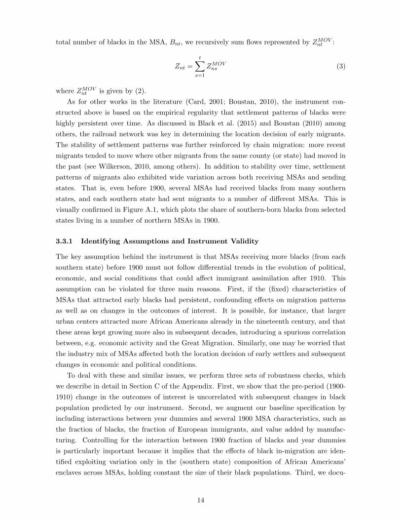
total number of blacks in the MSA, Bnt, we recursively sum flows represented by ZMOVnt :

Znt =

t∑s=1

ZMOVns (3)

where ZMOVnt is given by (2).

As for other works in the literature (Card, 2001; Boustan, 2010), the instrument con-

structed above is based on the empirical regularity that settlement patterns of blacks were

highly persistent over time. As discussed in Black et al. (2015) and Boustan (2010) among

others, the railroad network was key in determining the location decision of early migrants.

The stability of settlement patterns was further reinforced by chain migration: more recent

migrants tended to move where other migrants from the same county (or state) had moved in

the past (see Wilkerson, 2010, among others). In addition to stability over time, settlement

patterns of migrants also exhibited wide variation across both receiving MSAs and sending

states. That is, even before 1900, several MSAs had received blacks from many southern

states, and each southern state had sent migrants to a number of different MSAs. This is

visually confirmed in Figure A.1, which plots the share of southern-born blacks from selected

states living in a number of northern MSAs in 1900.

3.3.1 Identifying Assumptions and Instrument Validity

The key assumption behind the instrument is that MSAs receiving more blacks (from each

southern state) before 1900 must not follow differential trends in the evolution of political,

economic, and social conditions that could affect immigrant assimilation after 1910. This

assumption can be violated for three main reasons. First, if the (fixed) characteristics of

MSAs that attracted early blacks had persistent, confounding effects on migration patterns

as well as on changes in the outcomes of interest. It is possible, for instance, that larger

urban centers attracted more African Americans already in the nineteenth century, and that

these areas kept growing more also in subsequent decades, introducing a spurious correlation

between, e.g. economic activity and the Great Migration. Similarly, one may be worried that

the industry mix of MSAs affected both the location decision of early settlers and subsequent

changes in economic and political conditions.

To deal with these and similar issues, we perform three sets of robustness checks, which

we describe in detail in Section C of the Appendix. First, we show that the pre-period (1900-

1910) change in the outcomes of interest is uncorrelated with subsequent changes in black

population predicted by our instrument. Second, we augment our baseline specification by

including interactions between year dummies and several 1900 MSA characteristics, such as

the fraction of blacks, the fraction of European immigrants, and value added by manufac-

turing. Controlling for the interaction between 1900 fraction of blacks and year dummies

is particularly important because it implies that the effects of black in-migration are iden-

tified exploiting variation only in the (southern state) composition of African Americans’

enclaves across MSAs, holding constant the size of their black populations. Third, we docu-

14

ment that our findings are unchanged when including a measure of predicted industrialization

constructed by interacting 1900 industry shares in each MSA with national growth rates (see

also Sequeira, Nunn and Qian (Forthcoming) and Tabellini (Forthcoming)).

Second, one may be concerned that the instrument is spuriously correlated with changes in

the immigration regime induced by the Immigration Acts of the 1920s. While the quotas were

introduced at the national level, they likely had a differential effect across MSAs depending

on pre-existing ethnic composition (Collins, 1997; Ager and Hansen, 2017). We directly tackle

this issue by verifying that our instrument is not correlated with local exposure to the quotas,

as predicted by the distribution of pre-existing immigrant enclaves across MSAs. Moreover,

we provide evidence that our instrument is uncorrelated with changes in the average length

of stay of immigrants in the US, and has no direct effect on either the number or the national

composition of immigrants.

Third, the identifying assumption would be violated if outmigration from each southern

state were not independent of cross-MSA pull factors systematically related to 1900 settlers’

state of origin. We address this concern, formalized in Goldsmith-Pinkham, Sorkin and Swift

(2018) and Borusyak, Hull and Jaravel (2018), by examining the degree to which the in-

strument depends on variation coming from flows from a specific state to specific MSAs.

Reassuringly, both the strength of the instrument and our main results are unchanged when

separately interacting year dummies with the share of blacks born in each southern state,

i.e. α1900jn in (2). Note that, even if early settlements were as good as randomly assigned, one

remaining concern is that black outflows from each southern state, Ojt, might be differentially

affected by specific, time-varying shocks in northern destinations. To deal with this potential

threat, as in Boustan (2010), we construct a modified version of the instrument in (3) by

replacing Ojt with predicted (rather than actual) outmigration. We describe the construction

of this alternative instrument in detail in Section B of the Appendix, and only briefly review

the main steps in the next paragraph.

First, we predict outmigration from southern counties by exploiting only local demographic

and agricultural conditions at the beginning of each decade. Next, we aggregate these flows

to the state level to obtain the predicted number of blacks leaving each southern state j in

each decade, Ojt. Finally, we replace Ojt with Ojt in (2) to derive the (push-factors induced)

predicted number of blacks moving to city c in year t. By construction, this (predicted)

measure of black outmigration from the South is orthogonal to any specific shock occurring in

the North. Moreover, by exploiting southern shocks to agricultural conditions, this alternative

instrument is less likely to suffer from the problem of high serial correlation in migration

patterns between sending and receiving areas – a possible concern for standard shift-share

instruments (Jaeger, Ruist and Stuhler, 2018). Both first stage and 2SLS results are robust

to using this, instead of our baseline version of the instrument.

3.4 First Stage

Table 2 reports first stage results for the relationship between the actual number of blacks

and the instrument constructed in (3). Column 1 controls for total MSA population, and

15

includes MSA and year fixed effects. Column 2 presents our preferred specification, and

augments the set of controls included in column 1 by interacting year dummies with region

dummies. There is a strong and positive relationship between the instrument and the number

of blacks, and the F-stat is above conventional levels. A coefficient as in column 2 implies

that every predicted new black arrival in the MSA is associated with 1.1 more actual black

residents. These estimates are very similar to those reported in Shertzer and Walsh (2016) and

in Tabellini (2018) for the same historical period, for neighborhoods and cities, respectively.

They are instead an order of magnitude smaller than those obtained in Boustan (2010), who

focuses on the second wave of the Great Migration. Figure 3 plots the graphical analogue of

the regression estimated in column 2, and verifies the strong relationship between the actual

and the predicted number of blacks.

Subsequent columns of Table 2 explore the robustness of results reported in column 2.

First, we show that our estimates are not sensitive to running unweighted regressions (col-

umn 3).7 Next, we augment our baseline specification by interacting year dummies with,

respectively, the 1900 fraction of blacks, the 1900 fraction of immigrants, the log of 1900

output in manufacturing, and the fraction of men aged 15–64 employed in manufacturing

(columns 4 to 7). In all cases, the coefficient remains quantitatively close to that reported in

column 2, and its statistical significance is not affected.

In Appendix Figure C.3 we plot the first stage coefficient for regressions that include,

respectively, interactions between year dummies and the share of blacks born in each southern

state, i.e. α1900jn in equation (2). Reassuringly, the point estimate always remains highly

significant and very similar to that obtained from our baseline specification (Table 2, column

2), which is the first point estimate on the left in Figure C.3.

Finally, Table C.7 replicates the exercise in Table 2 using the version of the instrument

that relies on southern push factors to predict net black migration rates. While smaller in

magnitude, the relationship between actual and predicted number of blacks is always strong

and statistically significant, and the F-statistic remains high.

Overall, the pattern presented in this section suggests that there is a strong relationship

between the actual and the predicted number of blacks, which is robust to the inclusion of

several controls and the use of alternative specifications.

4 Results

In this section we present our main results on the effects of the Great Migration on immi-

grant assimilation. First, we show that the inflow of blacks increased successful assimilation,

measured as intermarriage between immigrants and native-born whites and occupational up-

grading (Section 4.1). Second, we document that black in-migration raised the share of

7In our main analysis we estimate individual level regressions. This is equivalent to running MSA-levelregressions, weighted by the number of immigrants.

16

immigrants who were naturalized citizens, and induced foreign born parents to give more

American sounding names to their children, suggesting that immigrants responded to black

arrivals by increasing their assimilation efforts (Section 4.2). We conclude by performing

several robustness checks (Section 4.3).

4.1 Social and economic assimilation

In Panel A of Table 3, we study the effects of the Great Migration on equilibrium measures of

assimilation. Our most preferred proxy for assimilation success is intermarriage between im-

migrants and native-born whites, which captures not only immigrants’ desire to Americanize,

but also native-born whites’ willingness to accept immigrants as part of their group. Re-

stricting attention to married immigrant men, we define the dependent variable as a dummy

equal to one for being married with a native-born white of native-born parentage. We start

by estimating equation (1) with OLS: column 1 only includes MSA and year fixed effects,

and controls for individual level characteristics (age, origin region, and years in the U.S. fixed

effects), whereas column 2 also includes year by region fixed effects. In both cases, the point

estimate is positive, but close to zero and not statistically significant.

From column 3 onwards, we present 2SLS results. Column 3 replicates column 2 instru-

menting the number of blacks with the shift-share instrument introduced in Section 3.3. The

coefficient is now larger in magnitude and statistically significant at the 5% level. The down-

ward bias in the OLS estimates indicates that black migrants may have selected into MSAs in

which the prospects for immigrant assimilation were not that bright. The point estimate in

column 3 implies that one standard deviation increase in the number of blacks (approximately

45,000 people) increases intermarriage rates by 0.54 percentage points, or 7.5% of the 1910

mean. For a large recipient city like Chicago, that received close to 230,000 blacks during the

period, this effect amounts to 2.74 percentage points, or 57.1% of the 1910 mean.

In columns 4 and 5, we gradually add a more stringent set of controls – respectively,

MSA by region of origin, and year by region of origin fixed effects – but, reassuringly, both

the magnitude and the precision of the coefficient are left unchanged. Finally, in column 6,

we present results for the linked sample of immigrants who always stayed in the same MSA

between 1910 and 1930. Results remain qualitatively in line with those reported in columns

3 to 5, but become larger in magnitude and less precisely estimated.

Our main results focus on social assimilation. Table D.1 in the Appendix presents results

for manufacturing employment, as a proxy of economic status. Employment in manufacturing

drops significantly in response to large inflows. Estimates imply that one standard deviation

increase in the number of African Americans lowers the share of immigrants working in the

manufacturing sector by 2.5 percentage points, or 10% relative to the 1910 mean. Immigrants

were almost twice as likely as native-born whites to be employed in manufacturing during the

period under study. We thus interpret these findings as reflecting economic assimilation, with

foreign born men moving out of the immigrant-intensive sector.

In Appendix Section D we also consider a number of additional outcomes capturing eco-

nomic and social assimilation. Confirming the results on manufacturing employment, we find

17

a reduction in the share of immigrants who were unskilled, again suggesting that immigrants

were able to improve their socio-economic status because of the Great Migration (Column

2 of Table D.2). The inflow of blacks did not substantially impact immigrants’ employment

probabilities, suggesting that, if there was labor market competition between immigrants and

blacks, its effects were muted, perhaps as a result of immigrants’ socio-economic advancement

(Column 3 of Table D.2).8 Black inflows also reduced ethnic residential segregation, but these

effects are small and never precisely estimated.

4.2 Assimilation Effort

We next analyze immigrant effort. In Panel B of Table 3, the dependent variable is a dummy

equal to one for being a naturalized citizen, our main proxy for immigrant assimilation ef-

fort. As in Panel A, columns 1 and 2 report OLS results, while subsequent columns present

2SLS estimates from the repeated cross-sections (columns 3 to 5) and the linked (column 6)

datasets. In all cases, the point estimate is positive and statistically significant, suggesting

that black inflows increased the effort exerted by the foreign-born to integrate in American

society. According to our most preferred specification, reported in column 5, one standard

deviation increase in black population raises naturalization rates by approximately 1.5 per-

centage points, or by 3.5% relative to the 1910 mean. When using the linked sample (column

6), the effect becomes more precisely estimated and substantially larger. Regressions in the

linked sample are estimated in the restricted set of people who were not naturalized in the

previous decade. That we restrict attention to the group at risk can explain why estimated

coefficients are larger in magnitude in the linked sample for both intermarriage and natural-

ization rates.

As an alternative proxy for immigrant effort, in Panel B of Appendix Table D.1, we

consider the names chosen by immigrant parents for their children. In line with results

reported in Table 3, there is a negative and statistically significant effect of black inflows on

the foreign name index. The magnitude of the effect is substantial. It implies that the inflow

of 100,000 blacks – or, less than half of those received by Chicago – led to a change in Italian

names equivalent to that from Luciano to Mike, and a change in Russian names equivalent to

that from Stanislav to Morris or Max.

Overall, results in this section suggest that the arrival of African Americans, induced

foreign born individuals to exert more effort to assimilate. As we show in Section 5 below,

these average effects mask substantial heterogeneity. Before discussing the mechanisms, in the

next section, we summarize a number of checks that test the robustness of our main results.

8It is also possible that black workers were substitutes for some immigrant groups but complements toothers, and that the null effects reported in Table D.2 were due to opposite effects which, on average, canceledeach other out. In Section 5 we return to this point and explore the heterogeneity of the economic impact ofblack inflows across immigrant groups.

18

4.3 Summary of Robustness Checks

We summarize here the robustness checks we conduct to address concerns regarding the

validity of our identification strategy. A detailed description of these checks can be found in

Section C of the Appendix.

To show that 1900 black settlements are unlikely to be correlated with time-varying char-

acteristics of MSAs that could have affected assimilation patterns we perform three checks: (i)

we show that the 1900 to 1910 change in European immigration is uncorrelated with predicted

black inflows between 1910 and 1930 (Figure C.1), (ii) we formally demonstrate the absence

of pre-trends for our outcome variables (Table C.1), (iii) we show that our results are robust

to interacting year dummies with a number of 1900 MSA characteristics, including the 1900

share of blacks at the MSA (Table C.2), and (iv) we document that results are unchanged

when separately controlling for a (predicted) measure of industrialization.

To specifically tackle the concern that blacks moved to northern MSAs more affected by

the 1920s immigration quotas – and that this spurious correlation is not dealt with by our

instrument – we construct a measure of “quota exposure” for each MSA, by interacting region-

of-origin-specific immigration restrictions with pre-existing settlements in the MSA (Ager and

Hansen, 2017). Using this variable, we document that our instrument is uncorrelated with the

number of “missing” immigrants that an MSA would have received had immigration restric-

tions not been introduced (Figure C.2). We also verify that black in-migration is uncorrelated

with changes in immigrants’ average length of stay in the US (Table C.3).

We then turn to the possibility that our results might be driven by compositional changes

in the immigrant population, triggered by black arrivals. The robustness of our results to the

use of the linked sample already mitigates this concern. We perform three additional checks:

we show that black inflows did not affect (i) the number of international immigrants in the

MSA (Table C.4), (ii) the ethnic composition of immigrants, measured as shares of different

origin regions over total MSA foreign population (Table C.5), or (iii) sex ratios within the

immigrant group, either for younger or for older immigrants (Table C.6).

To address concerns related to the validity of Bartik instruments, as detailed in Goldsmith-

Pinkham, Sorkin and Swift (2018), we show that both our first stage (Figure C.3) and 2SLS

results (Figure C.4) are robust to interacting year dummies with the share of southern-born

blacks from each state, i.e. the Bartik weights. Next, to show that time-specific shocks in

northern MSAs are unlikely to have driven outmigration flows from the South, we replicate

our results using a push version of the instrument, following Boustan (2010) (Tables C.7 and

C.8). Finally, we show that neither first stage nor 2SLS results are sensitive to the exclusion

of outliers (Figures C.5 and C.6).

5 Mechanisms

Section 4 showed that, along important social and economic dimensions, black in-migration

fostered the assimilation of European immigrants. We find evidence both for increased im-

migrant efforts and for increased assimilation as observed in equilibrium outcomes. In this

19

section, we explore mechanisms that may have generated these effects. We start by examining

whether higher assimilation was driven by economic forces, such as labor market competition

and skill complementarities between immigrants and African Americans. While we find some

supporting evidence for such economic pathways, these alone cannot explain all our findings.

We argue instead for a role of social channels in driving observed responses to the Great

Migration, and provide empirical evidence consistent with such an interpretation.

5.1 Economic mechanisms

Blacks who moved to the North between 1910 and 1930 were disproportionately low-skilled and

were absorbed in sectors that were until then immigrant-dominated. The ensuing competition

between low-skilled workers and blacks has been highly emphasized in the historical literature

(Collins and Wanamaker, 2015; Boustan, 2016). Violent conflict between ethnic minorities

and African Americans was common, and even predated the Great Migration (Rieder, 1987;

McDevitt, Levin and Bennett, 2002; Cho, 1993). Already before the Civil War, Irish immi-

grants reacted to their deplorable living conditions in northern cities with resentment against

blacks, which was demonstrated in practice through their participation in anti-abolitionist

riots and mobbing of African Americans (Ignatiev, 1995).

Competition with blacks might have induced immigrants to either invest in skill acquisi-

tion or actively try to differentiate themselves from their competitors, perhaps by signaling

their Americanization as an asset in order to become more attractive to employers. Skill

acquisition leading to occupational upgrading seems unlikely, since it would have implied,

counterintuitively, that immigrants could have invested in their human capital and advanced

occupationally even prior to the Great Migration, but they chose not to do so. Signaling

American identity as a means to deal with competition is instead a channel that has been

highlighted by the historical literature (Olzak and Shanahan, 2014). Ignatiev (1995), in his

book How the Irish became white, documents how the Irish before the civil war facilitated

their assimilation by emphasizing their differences from African Americans. Roediger (1999)

shows how “immigrants in dirty and disease-ridden cities countered nativist assertions of racial

difference with a determined focus on their own whiteness, on “the Negro”, and on slavery”

(Guterl, 2001).

To examine whether competition with blacks may have been the driver of immigrant

assimilation, we plot heterogeneous responses across immigrant groups in Figure 4. We report

2SLS coefficients for the effects of the Great Migration on the probability of naturalization (left

panel) and intermarriage (right panel). Regression results underlying Figure 4 are reported

in Table A.4. With the exception of the UK, immigrants from new source regions (Russia

and Eastern and Southern Europe) exhibit the highest increase in naturalization rates. On

the contrary, immigrants from old sending countries (Germany and Northern and Western

Europe) experience smaller or negative changes. These heterogeneous effects are consistent

with increased efforts for groups most likely to experience labor market or other forms of

competition from incoming blacks, and who might have used naturalization as a means to

20

signal an American identity.9

However, if competition were the main channel driving results, we should also observe the

largest increases in assimilation rates among groups that increased their efforts the most. This

does not appear to be the case. Social assimilation, as proxied by intermarriage rates follows

the opposite pattern from naturalization rates. While effects are positive for most groups,

with the notable exception of the Irish, acceptance by the native-born group increases the

most for old source country nationals. One potential explanation for the heterogeneous pat-

terns displayed in Figure 4 is that they resulted from labor market complementarity between

immigrants and African Americans.

We next investigate the role of labor market competition more directly. Table 5 presents

interactions of black inflows with the share of an immigrant group at the MSA-level employed

in manufacture (columns 1 and 2) or in unskilled occupations (columns 3 and 4) in 1900,

prior to the Great Migration. The positive effect of black inflows on naturalization rates

seems to stem entirely from groups of immigrants employed in these sectors and that were

disproportionately exposed to black competition. This confirms the origin region-level results

of Figure 4, and suggests that labor market exposure to black migrants induced immigrants

to increase their assimilation efforts. The effect of employment sector on intermarriage rates

on the other hand is muted, suggesting that competition may have driven assimilation efforts,

but not actual assimilation.

We then turn to the potential role of labor market complementarities between immigrants

and blacks. If immigrants exhibited some degree of complementarity with African Ameri-

cans, black arrivals may have not constituted direct competition, but instead may have led

to immigrants’ occupational upgrading (Peri and Sparber, 2009; Foged and Peri, 2016). Such

economic advancement could then have fostered Europeans’ social incorporation. Figure A.2

shows that the skills of African Americans were very similar to those of Eastern and Southern

Europeans, but quite different from those of more skilled native-born whites and immigrants

from old source countries. It is possible that the heterogeneity patterns observed for so-

cial assimilation, with Northern and Western Europeans exhibiting the highest increases in

intermarriage, are a result of blacks (positively) affecting immigrants’ economic status.

If economic complementarities were the main drivers of our results, we would expect similar

patterns of heterogeneity for economic outcomes. This is not what we find. Figure 5 presents

the effects of black inflows, separately for each immigrant group, on economic outcomes.10 In

the left panel we consider the employment share of immigrants in manufacturing – a sector

where the majority of immigrants used to be employed, but where much fewer native-born

whites were working. This was also a sector that absorbed many African Americans during the

9The patterns in Figure 4 are not driven by differential responses of immigrant groups of different size.Results (not reported for brevity) are robust to controlling for the share of each immigrant origin group in1900 interacted with year fixed effects.

10Underlying regressions are shown in Table A.5.

21

Great Migration (e.g. Boustan, 2016). In the right panel we construct the native-immigrant

gap in log occupational scores.11 Unlike social assimilation, economic assimilation displays

little heterogeneity, and does not indicate that old source immigrants were favored by the

Great Migration relative to new ones. The reduction in the share of immigrants employed

in manufacturing is rather uniform across groups and there is no clear trend in the effects

of black inflows on the native-immigrant gap in occupational scores across ethnic groups. In

fact, if anything, the gap becomes larger for Germans, contrary to what one would expect if

skill complementarities were driving immigrant assimilation.12 Taken together, the results in

Figure 5 suggest that the patterns observed for intermarriage are unlikely to be mediated by

differential economic advancement for the English, Western and Northern Europeans.

5.2 Social mechanisms

If the channels of economic competition and labor market complementarities are unable to

explain all of our findings, what other mechanism could generate the observed effects? Here

we propose and test empirically the idea that the arrival of African Americans made European

immigrants, who were previously viewed as members of a social and cultural outgroup, appear

“white” in the eyes of native-born individuals (Ignatiev, 1995; Jacobson, 1999). This, in turn,

favored their inclusion into the native-born white majority. We formalize this idea in a simple

model and present empirical evidence consistent with the model’s predictions.

5.2.1 Conceptual framework

An extensive historical literature suggests that the Great Migration catalyzed the assimilation

of immigrants and substantially contributed to their Americanization. One factor emphasized

throughout this literature is the role of changing perceptions of native-born whites toward

racial boundaries in propelling this assimilation (Ignatiev, 1995; Guterl, 2001). With the

arrival of African Americans, skin color became a salient determinant of racial distinctions,

and this eased the path to inclusion into the native-born majority for white Europeans.

The early decades of the 20th century were dominated by academic theories about race

and eugenics that emphasized fine grained racial distinctions among the various European

groups. Madison Grant, the author of the opus magnum of scientific racism, The Passing of

the Great Race, and one of the intellectuals behind the design of the immigration restrictions

of the 1920s, proclaimed Americans to be “Nordics”, the race of “the Homo Europaeus, the

white man par excellence” (Spiro, 2008). Below the Nordic man, in the hierarchy of races,

followed the Alpines and Mediterraneans – the color of the former being described as “fair

to dark”, and that of the latter as “swarthy”. Grant and his followers were worried that the

11Occupational scores assign to an individual the median income of his job category in 1950, and can beused as a proxy for lifetime earnings (Abramitzky, Boustan and Eriksson, 2014).

12As for Figure 4, the results in Figure 5 are robust to controlling for the share of each immigrant origingroup in 1900 interacted with year fixed effects.

22

Nordic type in the US was being “elbowed out of his own home” and “literally driven off the

streets of New York City by the swarms of Polish Jews.”

The Great Migration shifted the focus, both of academics and of society at large, from

ethnic differences to color as a racial group identifier. Lothrop Stoddard, another prominent

eugenicist and Klansman, and author of the best-seller The Rising Tide of Color against

White World Supremacy, emphasized how color-coding race would lead to assimilation and

unification of ethnic and cultural differences in the US. At the same time, race riots in northern

cities contributed to the framing of blacks as the primary social threat – the emerging “Negro

problem” (Guterl, 2001). The salience of race reduced ethnic prejudice, and made it easier

for immigrants to assimilate into the US society.

Building on these historical insights, we construct a simple model to explain our findings.

We present the formal framework in Appendix Section E, and provide a summary here. The

framework draws from the cognitive psychology literature on categorization (Turner et al.,

1987) and from related work in economics (Shayo, 2009). We start from the assumption

that ethnic and racial groups are ranked in terms of their distance, social, cultural, or other,

from native-born whites.13 Native-born whites in turn engage in taste-based discrimination

in order to avoid the psychological costs of interaction with outgroup members. These costs

are increasing in the outgroup’s average perceived distance, which is context dependent. In

particular, the appearance of an outgroup of higher actual distance to natives from that

of existing outgroups reduces perceived distance and leads to the recategorization of some

outgroup members as members of the ingroup.14 This process of context-dependent catego-

rization, known as meta contrast principle, is a central tenet of the self categorization theory

in social psychology (Turner et al., 1987, 1994), and is documented in experimental studies

(Tajfel and Wilkes, 1963). Fryer and Jackson (2008) show that such a classification rule can

derive from a utility maximization problem.15

The role of relative perceived distance is also consistent with the historical narrative on

the progressive incorporation of European immigrants into the white Anglo-Saxon majority.

In his study of this process, for example, Jacobson (1999) states that “In racial matters

above all else, the eye that sees is ‘a means of perception conditioned by the tradition in

which its possessor has been reared.’ The American eye sees a certain person as black, for

instance, whom Haitian or Brazilian eyes might see as white. Similarly, an earlier generation

of Americans saw Celtic, Hebrew, Anglo-Saxon, or Mediterranean physiognomies where today

13For recent works measuring cultural distance see Bertrand and Kamenica (2018) and Desmet and Wacziarg(2018).

14Similar predictions on reclassification are delivered by the literature on stereotypes (Bordalo et al., 2016),which relies on the representativeness heuristic (Kahneman and Tversky, 1974). Stereotypes about groupsdepend on the reference group. Irish immigrants may be thought of primarily as Catholic when comparedto native-born Anglo-Saxons. However, when compared to African Americans, they are more likely to beperceived as white, since skin color is the dimension in which Irish and African Americans differ the most.

15Gennaioli and Tabellini (2018) rely on the meta contrast principle to study political identities.

23

we see only subtly varying shades of a mostly undifferentiated whiteness.”

In this context, black inflows in the North increase the outgroup’s average distance from

native whites. There is little doubt that African Americans stood at the bottom of the

social hierarchy in early 20th century US and were thus more distant to native whites than

European immigrants (Myrdal, 1944). Their appearance reduced the perceived distance of

native whites from European immigrants, allowing the incorporation of the latter to American

society. In response to the changed attitudes of whites, immigrants exerted more effort to

assimilate, because reduced barriers to integration now implied that that additional effort

could pay off. This was especially true for immigrant groups of intermediate distance to

native whites. Immigrants of ambiguous racial classification, such as the Eastern and Southern

Europeans, were discriminated prior to the Great Migration, but were seen more favorably

after black arrivals. Instead, nationalities that were culturally closer to native whites, such

as Northern and Eastern Europeans, could now be integrated with less effort than before. At

the same time, the recategorization effect of black inflows would not have affected non-white

immigrant groups, who were sufficiently distant from native whites, and who would not have

been accepted as part of native society despite any increase in their assimilation efforts. The

main prediction of our framework is thus an inverted U-shaped relationship between distance

and assimilation outcomes in response to the Great Migration.

5.2.2 Empirical evidence on social channels

Anti-immigrant sentiment and immigrant stereotypes in the press. The first piece of

evidence for a mechanism emphasizing lower relative distance and reduced prejudice towards

European immigrants comes from the historical press. Newspaper language and sentiment

largely responds to readers’ demands (Gentzkow and Shapiro, 2010) and thus anti-immigrant

sentiment in local newspapers should capture the public’s attitudes toward immigrants in

each MSA. We compile a list of articles from Newspapers.com, covering cities in 69 of the

108 MSAs in our sample. In particular, we compute the MSA-level frequency of immigration-

related terms appearing in local newspapers and investigate how that responds to the Great

Migration. Results are presented in Table 4. The dependent variable is constructed as the

number of articles containing the expression at the top of each column, scaled by the total

number of articles containing the word “and” in newspapers of a given MSA in a given decade.

To ease interpretation, the dependent variable is standardized by subtracting the mean and

dividing by the standard deviation in 1910.

The inflow of African Americans had a negative and marginally significant effect on generic

terms related to immigration (“immigration”; “immigrants”; “aliens”), suggesting that black

arrivals lowered the salience of the immigration issue (column 1). Next, to more directly test

our proposed mechanism, we focus on terms that either reflect concerns over immigration or

capture cultural or ethnic prejudice. In column 2, we show that the Great Migration had

a negative and statistically significant effect on the relative frequency of the term “quotas”.

Consistent with our previous findings, this result indicates that demand for immigration re-

strictions fell as European immigrants became increasingly perceived as less distant to native-

24

born whites. In line with this idea, black inflows reduced the relative frequency of the word

“Dago” (column 3), which was often used when describing Italian immigrants in disparaging

terms.

In columns 4 to 6 we document that mentions to both “Catholic” or “Catholic threat”

(columns 4 and 5) and the Ku Klux Klan (column 6) fell in response to black in-migration.

At the beginning of the 20th century, and especially during the 1920s, religion was a highly

salient issue, and nativism was often associated with anti-Catholicism (see Higham (1998)

and D’Amico and Tabellini (2018), among others). Indeed, the revival of the KKK that took

place during the 1920s did not have an anti-black but, rather an anti-Catholic focus (Dumenil,

1991). Hence, we interpret findings in columns 4, 5, and 6 as consistent with the idea that the

Great Migration softened the widespread anti-immigration sentiments (in particular towards

Catholic immigrants) prevailing at the time. The decline in KKK mentions reported in column

6 likely represents a lower bound for the effects of black inflows on the reduction in native-born

whites’ prejudice towards European immigrants, since the arrival of African Americans likely

increased KKK activity.

Alongside prejudice towards immigrants, the inflow of African Americans also reduced

stereotyping. We provide evidence for this by searching for the co-occurrence of words stereo-

typically associated with two of the largest European immigrant groups of the time, the Irish

and the Italians. Figure 6 and Table A.3 present 2SLS estimates from regressions where the

dependent variable is the relative frequency of such co-occurrences. In the left panel of Fig-

ure 6 we normalize each frequency with the frequency of the word “and”, which is proxying

for the total number of articles published in an MSA in a decade. Black inflows reduced the

probability that the Irish and Italians were mentioned jointly with the term “Catholic”. This

lends support to a theoretical mechanism whereby immigrants are reclassified as ingroup mem-

bers, and are no longer associated with features that previously distinguished them from the

native-born whites, such as religion. This pattern is also consistent with context-dependent

stereotyping, as in Bordalo et al. (2016). Similarly, the relative frequency of other stereotypi-

cal associations – such as that of the Irish with violence, or that of the Italians with the mafia

– also declined following black in-migration.

The right panel of Figure 6 normalizes the frequency of each co-occurrence with the

frequency of each stereotypical term. This is a complementary statistical test, since it requires

that the frequency of nationality-stereotypical term associations represents a smaller fraction

of the total mentions of a given stereotypical term, and thus controls for the fact that terms like

“crime” or “alcohol” may have become less widely discussed topics over time. The qualitative

message is unchanged: also in this case, the Irish were significantly less likely to be associated

with Catholicism, alcohol and crime, and Italians were significantly less likely to be associated

with the mafia. Overall, these results indicate that the Great Migration reduced native-born

whites’ propensity to link immigrants to negative stereotypes. Moreover, they indicate that

cultural traits like religion, which divided immigrants from natives, lost in importance.

Heterogeneity across immigrant groups. Our model predicts that the effect of the Great

Migration on immigrant assimilation effort should be non-monotonic in distance. Assimilation

25

outcomes should have been most positively affected for groups “at the margin”, who were

excluded before but who were given the opportunity to integrate once black inflows changed

native whites’ perceptions on ingroup boundaries.

We proxy for the distance between immigrants and native-born whites in two ways. First,

we use a measure of genetic distance from the UK, compiled by Spolaore and Wacziarg (2009).

Second, we rely on the measure of linguistic distance from English constructed by Chiswick and

Miller (2005). The latter measure assigns lower values to languages in which English speakers

had reached a higher degree of proficiency after several weeks of instruction. In Table 6, we

examine if the effect of black inflows varies non-linearly with these two measures of distance

at the nationality level. Figure 7 plots the implied effect of black inflows on intermarriage

(left) and naturalization (right), by values of genetic (upper panel) and linguistic distance

(lower panel) respectively.

Using either measure of distance, we observe an inverted U-shaped pattern for natural-

ization rates. Results are less clear in the case of intermarriage rates, though still present in

the case of genetic distance. Consistent with our model, the inverted U-shaped pattern is ob-

served primarily for effort. Changed native whites’ perceptions of relative distance now make

it profitable for immigrant groups of intermediate cultural distance to invest in assimilation

effort and integrate into American society.16

Finally, in Table A.6 in the Appendix, we present results for our main outcomes for non-

white immigrants (Mexicans and Chinese) who were viewed as even farther away in distance

from native-born whites. For these very distant groups there is indeed no effect of black

inflows on either assimilation effort or actual assimilation.

Ruling out other alternatives. We conclude by exploring two potential alternative mecha-

nisms, and find little evidence consistent with either of them. First, we consider the possibility

that black arrivals altered politicians’ incentives, inducing them to shift their rhetoric from its

previous anti-immigrant nativist focus to concerns related to the changing racial composition

and its concomitant dangers, such as crime. We provide evidence against this mechanism

by showing that black inflows did not increase immigrants’ employment in the public sector

(Table A.7) – either overall (column 1) or in specific occupations, such as firemen or policemen

(columns 2 and 3). These patterns suggest that our main results are not driven by immigrants

being able to advance economically and socially by directly benefitting from patronage jobs.

Second, black arrivals might have increased immigrants’ incentives to mobilize and push for

political inclusion. The labor movement and unionization represented one of the most common

forms of social mobilization at the time. Since blacks likely increased labor market competition

mostly for Eastern and Southern Europeans, these immigrant groups might have been induced

to join local labor unions and eventually assimilate at a faster pace. However, as with the

16Genetic and linguistic distance may correlate with group size, but group size is not the driver of theobserved U-shaped pattern. Controlling for the share of each origin group in 1900 interacted with year fixedeffects leaves these results unchanged.

26

signaling scenario, without assuming a change in the attitudes of natives, this mechanism

can explain heterogeneous patterns for assimilation effort, but not for actual assimilation. In

Table A.8, we directly address this concern, and show that black inflows did not have any

significant effect on the presence of local chapters of the Industrial Workers of the World

(IWW), one of the largest industrial labor unions active in the US in the first decades of the

20th century. The IWW was founded in 1905 and data on IWW locals, collected as part of the

IWW history project at the University of Washington (Gregory, 2015), are available between

1906 and 1917. For this reason results in Table A.8 include only 1910 and 1920. To further

corroborate the validity of our empirical strategy, we also check that the local presence of IWW

unions in 1910 is uncorrelated with the 1910 to 1920 change in predicted black population

predicted (Figure A.3). This result rules out the possibility that early settlements of blacks

(and thus our instrument) were correlated with pre-determined labor and social mobilization,

which might have in turn favored the assimilation of European immigrants.

6 Conclusion

In this paper, we leverage plausibly exogenous variation in black inflows by exploiting 1900

settlements of southern-born blacks living outside the South, and the persistent nature of

migrant location decisions to show that the massive arrivals of African Americans to the US

North during the first Great Migration facilitated the assimilation of European immigrants

living in northern urban centers. We observe assimilation along dimensions that reflect in-

creased immigrant efforts, such as naturalization decisions and naming patterns, but also

equilibrium assimilation, such as intermarriage rates and occupational upgrading.

The effect of black infows on assimilation effort is highest for immigrant groups facing

labor market competition from incoming blacks. Social assimilation itself rather followed a

gradient of cultural distance that benefited the most integrated immigrant groups – primarily

old source country nationals. Groups sufficiently distant from native-born whites did not

exhibit a pronounced response to the Great Migration. Similar heterogeneity patterns are not

present for economic outcomes, suggesting a limited role for labor market complementarities.

To explain these effects, we build on insights from social psychology and formalize the

hypothesis – also proposed by the historical literature – that black inflows changed perceptions

of native-born whites toward Europeans, making this group seem “closer” to them than before.

Using measures of anti-immigrant sentiment from local historical newspapers, we provide

direct evidence that black in-migration reduced national stereotyping and lowered concerns

about immigration among native-born whites.

While one needs to be cautious when extrapolating these findings to other historical peri-

ods, we believe this study can provide answers to questions relevant today. To what extent has

the distinct racial profile of the US contributed to its multiculturalism and relative success in

integrating immigrants? Does the racial or cultural distance of new immigrant arrivals matter

for the assimilation of existing immigrant stock? The framework used here can be extended

to examine more broadly the interactions of earlier and later immigrant arrivals and the role

27

of new immigration on the assimilation of more established immigrant groups.

28

References

Abramitzky, Ran, and Leah Platt Boustan. 2017. “Immigration in American EconomicHistory.” Journal of Economic Literature, 55(4): 1311–45.

Abramitzky, Ran, Leah Platt Boustan, and Katherine Eriksson. 2014. “A Nation ofImmigrants: Assimilation and Economic Outcomes in the Age of Mass Migration.” Journalof Political Economy, 122(3): 467–717.

Abramitzky, Ran, Leah Platt Boustan, and Katherine Eriksson. 2018. “CulturalAssimilation during the Two Ages of Mass Migration.” Working Paper.

Ager, Philipp, and Casper Worm Hansen. 2017. “Closing Heavens Door: Evidencefrom the 1920s U.S.Immigration Quota Acts.” University of Copenhagen. Department ofEconomics Discussion Papers 17-22.

Akerlof, George A., and Rachel E. Kranton. 2000. “Economics and Identity.” QuarterlyJournal of Economics, 115(3): 715–753.

Alesina, Alberto, and Eliana La Ferrara. 2005. “Ethnic Diversity and Economic Perfor-mance.” Journal of Economic Literature, 43(3): 762–800.

Alesina, Alberto, Reza Baqir, and William Easterly. 1999. “Public Goods and EthnicDivisions.” Quarterly Journal of Economics, 114(4): 1243–84.

Algan, Yann, Thierry Mayer, and Mathias Thoenig. 2013. “The Economic Incentivesof Cultural Transmission: Spatial Evidence from Naming Patterns across France.” CEPRDiscussion Paper 9416.

Angrist, Josh. 2002. “How Do Sex Ratios Affect Marriage and Labor Markets? Evidencefrom America’s Second Generation.” Quarterly Journal of Economics, 117(3): 997–1038.

Atkin, David, Eve Colson-Sihra, and Moses Shayo. 2019. “How Do We Choose OurIdentity? A Revealed Preference Approach Using Food Consumption.” NBER WorkingPaper 25693.

Bandiera, Oriana, Imran Rasul, and Martina Viarengo. 2013. “The Making of Mod-ern America: Migratory Flows in the Age of Mass Migration.” Journal of DevelopmentEconomics, 102: 23–47.

Bandiera, Oriana, Myra Mohnen, Imran Rasul, and Martina Viarengo. Forthcom-ing. “Nation-Building Through Compulsory Schooling During the Age of Mass Migration.”Economic Journal.

Bauer, Michal, Christopher Blattman, Julie Chytilova, Joseph Henrich, EdwardMiguel, and Tamar Mitts. 2016. “Can War Foster Cooperation?” Journal of EconomicPerspectives, 30(3): 249–74.

Bazzi, Samuel, Arya Gaduh, Alexander D. Rothenberg, and Maisy Wong. 2019.“Unity in Diversity? How Intergroup Contact Can Foster Nation Building.” NBER WorkingPaper 25683.

Berry, John W., and Rudolf Kalin. 1979. “Reciprocity of Inter-Ethnic Attitudes in aMulticultural Society.” International Journal of Intercultural Relations, 3(1): 99–111.

Bertrand, Marianne, and Emir Kamenica. 2018. “Coming Apart? Cultural Distancesin the United States over Time.” NBER Working Paper 24771.

Biavaschi, Costanza, Corrado Giulietti, and Zahra Siddique. 2017. “The EconomicPayoff of Name Americanization.” Journal of Labor Economics, 35(4): 1089–1116.

Bisin, Alberto, and Thierry Verdier. 2001. “The Economics of Cultural Transmissionand the Dynamics of Preferences.” Journal of Economic Theory, 97(2): 298–319.

Black, Dan A., Seth G. Sanders, Evan J. Taylor, and Lowell J. Taylor. 2015. “TheImpact of the Great Migration on Mortality of African Americans: Evidence from the DeepSouth.” American Economic Review, 105(2): 477–503.

Bordalo, Pedro, Katherine Coffman, Nicola Gennaioli, and Andrei Shleifer. 2016.

29

“Stereotypes.” Quarterly Journal of Economics, 131(4): 1753–1794.Borjas, George J. 1987. “Self-Selection and the Earnings of Immigrants.” American Eco-

nomic Review, 77(4): 531–553.Borusyak, Kirill, Peter Hull, and Xavier Jaravel. 2018. “Quasi-Experimental Shift-

Share Research Designs.” NBER Working Paper 24997.Boustan, Leah Platt. 2010. “Was Postwar Suburbanization “White Flight”? Evidence from

the Black Migration.” Quarterly Journal of Economics, 125(1): 417–443.Boustan, Leah Platt. 2016. Competition in the Promised Land: Black Migrants in Northern

Cities and Labor Markets. Princeton:Princeton University Press.Boustan, Leah Platt, Matthew E. Kahn, and Paul W. Rhode. 2012. “Moving to

Higher Ground: Migration Response to Natural Disasters in the Early Twentieth Century.”American Economic Review, 102(3): 238–244.

Card, David. 2001. “Immigrant Inflows, Native Outflows, and the Local Labor MarketImpacts of Higher Immigration.” Journal of Labor Economics, 19(1): 22–64.

Card, David, Alexandre Mas, and Jesse Rothstein. 2008. “Tipping and the Dynamicsof Segregation.” Quarterly Journal of Economics, 123(1): 177–218.

Carneiro, Pedro Manuel, Sokbae Lee, and Hugo Reis. 2016. “Please Call me John:Name Choice and the Assimilation of Immigrants in the United States, 1900-1930.” IZADiscussion Paper 9792.

Chiswick, Barry R. 1978. “The Effect of Americanization on the Earnings of Foreign-BornMen.” Journal of Political Economy, 86(5): 897–921.

Chiswick, Barry R., and Paul W. Miller. 2005. “Linguistic Distance: A QuantitativeMeasure of the Distance between English and other Languages.” Journal of Multilingualand Multicultural Development, 26(1): 1–11.

Cho, Sumi K. 1993. “Korean Americans vs. African Americans: Conflict and Construction.”In Reading Rodney King: Reading Urban Uprising. , ed. Robert Gooding-Williams. NewYork:Routledge.

Collins, William J. 1997. “When the Tide Turned: Immigration and the Delay of the GreatBlack Migration.” Journal of Economic History, 57(3): 607–632.

Collins, William J., and Marianne H. Wanamaker. 2014. “Selection and Income Gainsin the Great Migration of African Americans.” American Economic Journal: Applied Eco-nomics, 6(1): 220–252.

Collins, William J., and Marianne H. Wanamaker. 2015. “The Great Migration inBlack and White: New Evidence on the Selection and Sorting of Southern Migrants.”Journal of Economic History, 75(4): 947–992.

D’Amico, Leonardo, and Marco Tabellini. 2018. “Immigration and Cultural Backlash inthe Age of Mass Migration: Evidence from Local Newspapers and Congressional Speeches.”Working Paper.

Derenoncourt, Ellora. 2019. “Can you Move to Opportunity? Evidence from the GreatMigration.” Working Paper.

Desmet, Klaus, and Romain Wacziarg. 2018. “The Cultural Divide.” NBER WorkingPaper 24630.

Duckitt, John H. 1994. The Social Psychology of Prejudice. Westport:Greenwood Press.Dumenil, Lynn. 1991. “The Tribal Twenties: “Assimilated” Catholics’ Response to Anti-

Catholicism in the 1920s.” Journal of American Ethnic History, 21–49.Echenique, Federico, and Roland G. Fryer, Jr. 2007. “A Measure of Segregation Based

on Social Interactions.” Quarterly Journal of Economics, 122(2): 441–485.Edin, Per-Anders, Peter Fredriksson, and Olof Aslund. 2003. “Ethnic Enclaves and

the Economic Success of Immigrants – Evidence from a Natural Experiment.” QuarterlyJournal of Economics, 118(1): 329–357.

30

Enos, Ryan D. 2017. The Space between Us: Social Geography and Politics. Cam-bridge:Cambridge University Press.

Eriksson, Katherine. 2018. “Ethnic Enclaves and Immigrant Outcomes: Norwegian Immi-grants during the Age of Mass Migration.” NBER Working Paper 24763.

Eriksson, Katherine, and Zachary A. Ward. 2018. “The Ethnic Segregation of Immi-grants in the United States from 1850 to 1940.” NBER Working Paper 24764.

Ferenczi, Imre, and Walter F. Willcox. 1929. International Migrations Volume I: Statis-tics. New York:National Bureau of Economic Research.

Ferrie, Joseph. 1996. “A New Sample of Males Linked from the Public Use Micro Sampleof the 1850 U.S. Federal Census of Population to the 1860 U.S. Federal Census ManuscriptSchedules.” Historical Methods, 29(4): 141–156.

Foged, Mette, and Giovanni Peri. 2016. “Immigrants’ Effect on Native Workers: NewAnalysis on Longitudinal Data.” American Economic Journal: Applied Economics, 8(2): 1–34.

Fouka, Vasiliki. 2019. “How do Immigrants Respond to Discrimination: The Case of Ger-mans in the US during World War I.” American Political Science Review, 113(2): 405–422.

Fouka, Vasiliki. Forthcoming. “Backlash: The Unintended Effects of Language Prohibitionin US Schools after World War I.” Review of Economic Studies.

Fryer, Roland, and Matthew O. Jackson. 2008. “A Categorical Model of Cognition andBiased Decision Making.” BE Journal of Theoretical Economics, 8(1).

Fryer, Roland G., and Steven D. Levitt. 2004. “The Causes and Consequences of Dis-tinctively Black Names.” Quarterly Journal of Economics, 119(3): 767–805.

Gaertner, Samuel, and John Dovidio. 2000. Reducing Intergroup Bias: The CommonIngroup Identity Model. New York:Psychology Press.

Gennaioli, Nicola, and Guido Tabellini. 2018. “Identity, Beliefs, and Political Conflict.”CEPR Discussion Paper 13390.

Gentzkow, Matthew, and Jesse M. Shapiro. 2010. “What Drives Media Slant? Evidencefrom U.S. Daily Newspapers.” Econometrica, 78(1): 35–71.

Gentzkow, Matthew, and Jesse M. Shapiro. 2011. “Ideological Segregation Online andOffline.” Quarterly Journal of Economics, 126(4): 1799–1839.

Goldin, Claudia. 1994. “The Political Economy of Immigration Restriction in the UnitedStates, 1890 to 1921.” In The Regulated Economy: A Historical Approach to Political Econ-omy. , ed. Claudia Goldin and Gary D. Libecap, 223–258. Chicago:University of ChicagoPress.

Goldsmith-Pinkham, Paul, Isaac Sorkin, and Henry Swift. 2018. “Bartik Instruments:What, When, Why, and How.” NBER Working Paper 24408.

Gordon, Milton A. 1964. Assimilation in American Life: The Role of Race, Religion, andNational Origins. New York:Oxford University Press.

Gregory, James N. 2005. The Southern Diaspora: How the Great Migrations of Black andWhite Southerners Transformed America. Chapel Hill:University of North Carolina Press.

Gregory, James N. 2015. “IWW History Project.” http://depts.washington.edu/iww/.Guglielmo, Thomas A. 2003. White on Arrival: Italians, Race, Color, and Power in

Chicago, 1890-1945. New York:Oxford University Press.Guterl, Matthew Pratt. 2001. The Color of Race in America, 1900-1940. Cam-

bridge:Harvard University Press.Hagendoorn, Louk. 1995. “Intergroup Biases in Multiple Group Systems: The Perception

of Ethnic Hierarchies.” European Review of Social Psychology, 6(1): 199–228.Haslam, S Alexander, Penelope J Oakes, John C Turner, and Craig McGarty. 1995.

“Social Categorization and Group Homogeneity: Changes in the Perceived Applicabilityof Stereotype Content as a Function of Comparative Context and Trait Favourableness.”

31

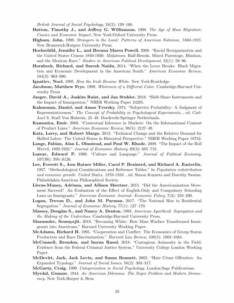
British Journal of Social Psychology, 34(2): 139–160.Hatton, Timothy J., and Jeffrey G. Williamson. 1998. The Age of Mass Migration:

Causes and Economic Impact. New York:Oxford University Press.Higham, John. 1998. Strangers in the Land: Patterns of American Nativism, 1860-1925.

New Brunswick:Rutgers University Press.Hochschild, Jennifer L., and Brenna Marea Powell. 2008. “Racial Reorganization and

the United States Census 1850-1930: Mulattoes, Half-Breeds, Mixed Parentage, Hindoos,and the Mexican Race.” Studies in American Political Development, 22(1): 59–96.

Hornbeck, Richard, and Suresh Naidu. 2014. “When the Levee Breaks: Black Migra-tion and Economic Development in the American South.” American Economic Review,104(3): 963–990.

Ignatiev, Noel. 1995. How the Irish Became White. New York:Routledge.Jacobson, Matthew Frye. 1999. Whiteness of a Different Color. Cambridge:Harvard Uni-

versity Press.Jaeger, David A., Joakim Ruist, and Jan Stuhler. 2018. “Shift-Share Instruments and

the Impact of Immigration.” NBER Working Paper 24285.Kahneman, Daniel, and Amos Tversky. 1974. “Subjective Probability: A Judgment of

Representativeness.” The Concept of Probability in Psychological Experiments, , ed. Carl-Axel S. Stael Von Holstein, 25–48. Dordrecht:Springer Netherlands.

Kamenica, Emir. 2008. “Contextual Inference in Markets: On the Informational Contentof Product Lines.” American Economic Review, 98(5): 2127–49.

Katz, Larry, and Robert Margo. 2013. “Technical Change and the Relative Demand forSkilled Labor: The United States in Historical Perspective.” NBER Working Paper 18752.

Lange, Fabian, Alan L. Olmstead, and Paul W. Rhode. 2009. “The Impact of the BollWeevil, 1892-1932.” Journal of Economic History, 69(3): 685–718.

Lazear, Edward P. 1999. “Culture and Language.” Journal of Political Economy,107(S6): S95–S126.

Lee, Everett S., Ann Ratner Miller, Carol P. Brainerd, and Richard A. Easterlin.1957. “Methodological Considerations and Reference Tables.” In Population redistributionand economic growth: United States, 1870-1950. , ed. Simon Kuznets and Dorothy Swaine.Philadelphia:American Philosophical Society.

Lleras-Muney, Adriana, and Allison Shertzer. 2015. “Did the Americanization Move-ment Succeed? An Evaluation of the Effect of English-Only and Compulsory SchoolingLaws on Immigrants.” American Economic Journal: Economic Policy, 7(3): 258–290.

Logan, Trevon D., and John M. Parman. 2017. “The National Rise in ResidentialSegregation.” Journal of Economic History, 77(1): 127–170.

Massey, Douglas S., and Nancy A. Denton. 1993. American Apartheid: Segregation andthe Making of the Underclass. Cambridge:Harvard University Press.

Mazumder, Soumyajit. 2018. “Becoming White: How Mass Warfare Transformed Immi-grants into Americans.” Harvard University Working Paper.

McAdams, Richard H. 1995. “Cooperation and Conflict: The Economics of Group StatusProduction and Race Discrimination.” Harvard Law Review, 108(5): 1003–1084.

McConnell, Brendon, and Imran Rasul. 2018. “Contagious Animosity in the Field:Evidence from the Federal Criminal Justice System.” University College London WorkingPaper.

McDevitt, Jack, Jack Levin, and Susan Bennett. 2002. “Hate Crime Offenders: AnExpanded Typology.” Journal of Social Issues, 58(2): 303–317.

McGarty, Craig. 1999. Categorization in Social Psychology. London:Sage Publications.Myrdal, Gunnar. 1944. An American Dilemma: The Negro Problem and Modern Democ-

racy. New York:Harper & Bros.

32

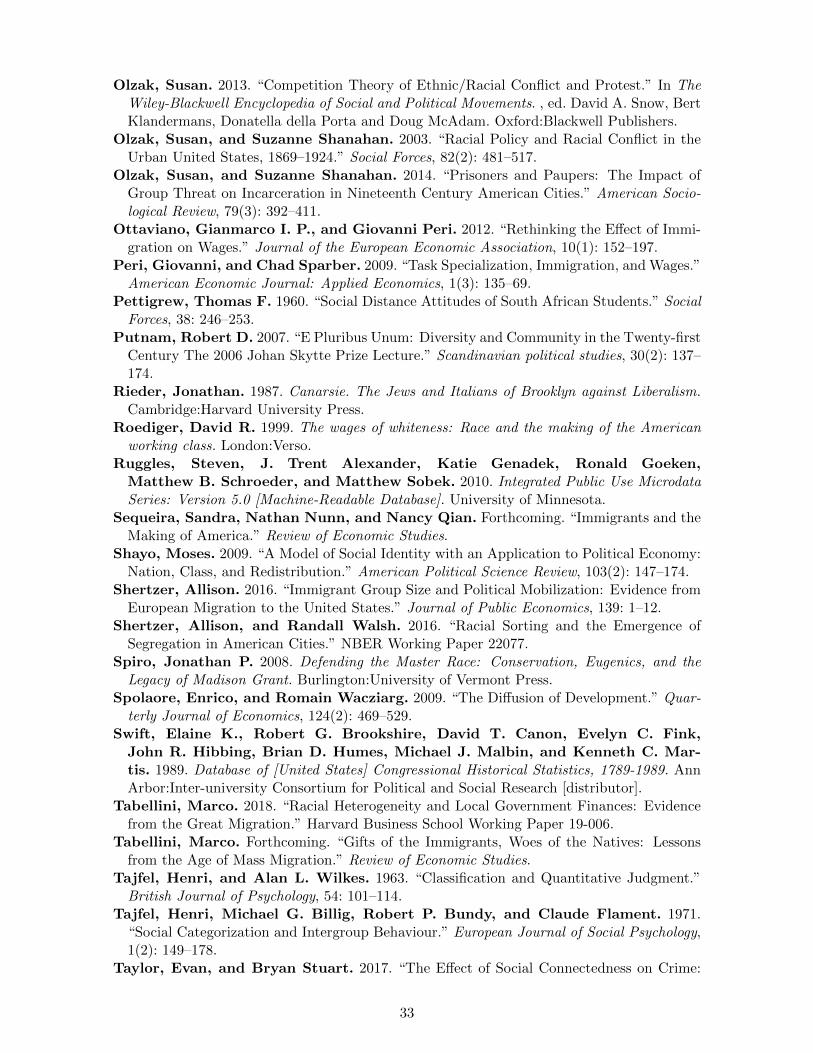
Olzak, Susan. 2013. “Competition Theory of Ethnic/Racial Conflict and Protest.” In TheWiley-Blackwell Encyclopedia of Social and Political Movements. , ed. David A. Snow, BertKlandermans, Donatella della Porta and Doug McAdam. Oxford:Blackwell Publishers.

Olzak, Susan, and Suzanne Shanahan. 2003. “Racial Policy and Racial Conflict in theUrban United States, 1869–1924.” Social Forces, 82(2): 481–517.

Olzak, Susan, and Suzanne Shanahan. 2014. “Prisoners and Paupers: The Impact ofGroup Threat on Incarceration in Nineteenth Century American Cities.” American Socio-logical Review, 79(3): 392–411.

Ottaviano, Gianmarco I. P., and Giovanni Peri. 2012. “Rethinking the Effect of Immi-gration on Wages.” Journal of the European Economic Association, 10(1): 152–197.

Peri, Giovanni, and Chad Sparber. 2009. “Task Specialization, Immigration, and Wages.”American Economic Journal: Applied Economics, 1(3): 135–69.

Pettigrew, Thomas F. 1960. “Social Distance Attitudes of South African Students.” SocialForces, 38: 246–253.

Putnam, Robert D. 2007. “E Pluribus Unum: Diversity and Community in the Twenty-firstCentury The 2006 Johan Skytte Prize Lecture.” Scandinavian political studies, 30(2): 137–174.

Rieder, Jonathan. 1987. Canarsie. The Jews and Italians of Brooklyn against Liberalism.Cambridge:Harvard University Press.

Roediger, David R. 1999. The wages of whiteness: Race and the making of the Americanworking class. London:Verso.

Ruggles, Steven, J. Trent Alexander, Katie Genadek, Ronald Goeken,Matthew B. Schroeder, and Matthew Sobek. 2010. Integrated Public Use MicrodataSeries: Version 5.0 [Machine-Readable Database]. University of Minnesota.

Sequeira, Sandra, Nathan Nunn, and Nancy Qian. Forthcoming. “Immigrants and theMaking of America.” Review of Economic Studies.

Shayo, Moses. 2009. “A Model of Social Identity with an Application to Political Economy:Nation, Class, and Redistribution.” American Political Science Review, 103(2): 147–174.

Shertzer, Allison. 2016. “Immigrant Group Size and Political Mobilization: Evidence fromEuropean Migration to the United States.” Journal of Public Economics, 139: 1–12.

Shertzer, Allison, and Randall Walsh. 2016. “Racial Sorting and the Emergence ofSegregation in American Cities.” NBER Working Paper 22077.

Spiro, Jonathan P. 2008. Defending the Master Race: Conservation, Eugenics, and theLegacy of Madison Grant. Burlington:University of Vermont Press.

Spolaore, Enrico, and Romain Wacziarg. 2009. “The Diffusion of Development.” Quar-terly Journal of Economics, 124(2): 469–529.

Swift, Elaine K., Robert G. Brookshire, David T. Canon, Evelyn C. Fink,John R. Hibbing, Brian D. Humes, Michael J. Malbin, and Kenneth C. Mar-tis. 1989. Database of [United States] Congressional Historical Statistics, 1789-1989. AnnArbor:Inter-university Consortium for Political and Social Research [distributor].

Tabellini, Marco. 2018. “Racial Heterogeneity and Local Government Finances: Evidencefrom the Great Migration.” Harvard Business School Working Paper 19-006.

Tabellini, Marco. Forthcoming. “Gifts of the Immigrants, Woes of the Natives: Lessonsfrom the Age of Mass Migration.” Review of Economic Studies.

Tajfel, Henri, and Alan L. Wilkes. 1963. “Classification and Quantitative Judgment.”British Journal of Psychology, 54: 101–114.

Tajfel, Henri, Michael G. Billig, Robert P. Bundy, and Claude Flament. 1971.“Social Categorization and Intergroup Behaviour.” European Journal of Social Psychology,1(2): 149–178.

Taylor, Evan, and Bryan Stuart. 2017. “The Effect of Social Connectedness on Crime:

33

Evidence from the Great Migration.” The George Washington University, Institute forInternational Economic Policy Working Papers 2017-24.

Tolnay, S., and E. M. Beck. 1990. “Black Flight: Lethal Violence and the Great Migration,1900 to 1930.” Social Science History, 14(3): 347–370.

Turner, John C., Michael A. Hogg, Penelope J. Oakes, Stephen D. Reicher, andMargaret S. Wetherell. 1987. Rediscovering the Social Group: A Self-CategorizationTheory. Cambridge:Basil Blackwell.

Turner, John C., Penelope J. Oakes, S. Alexander Haslam, and Craig McGarty.1994. “Self and Collective: Cognition and Social Context.” Personality and Social Psychol-ogy Bulletin, 20(5): 454–463.

United Nations, Department of Economic and Social Affairs, Population Division.2017. Trends in International Migrant Stock: The 2017 Revision. United Nations database,POP/DB/MIG/Stock/Rev.

Vigdor, Jacob L. 2010. From Immigrants to Americans: The Rise and Fall of Fitting In.Lanham:Rowman & Littlefield Publishers.

Watkins, Susan Cotts, ed. 1994. After Ellis Island: Newcomers and Natives in the 1910census. New York:Russell Sage Foundation.

Wilkerson, Isabel. 2010. The Warmth of Other Suns: The Epic Story of America’s GreatMigration. New York:Random House.

Wright, Gavin. 1986. Old South, New South. New York:Basic Books.

34

Figures and Tables

Figure 1. Effects of black inflows on intermarriage and naturalization rates

−.0

15

−.0

1−

.00

50

.00

5.0

1

Ma

rrie

d w

/ n

ative

−.2 −.1 0 .1 .2 .3

Predicted Black Inflows

−.0

2−

.01

0.0

1.0

2

Na

tura

lize

d

−.2 −.1 0 .1 .2 .3

Predicted Black Inflows

Binned scatterplot of the relationship between the change in the probability of marrying a native-born person

(left panel) or of being a naturalized citizen (right panel) and the change in predicted black population for the

years 1910-1930. Variables on the x- and y-axis represent residual changes, after partialling out total MSA

population, MSA and region by year fixed effects and indicators for age, nationality group and years in the

US. See Section 3.3 for details on the construction of the instrument for black population.

Figure 2. Immigrants and African Americans in sample MSAs

The map depicts the total number of foreign-born in 1910 (left panel) and the change in the number of African

Americans between 1910 and 1930 (right panel) in the 108 MSAs in our sample.

35

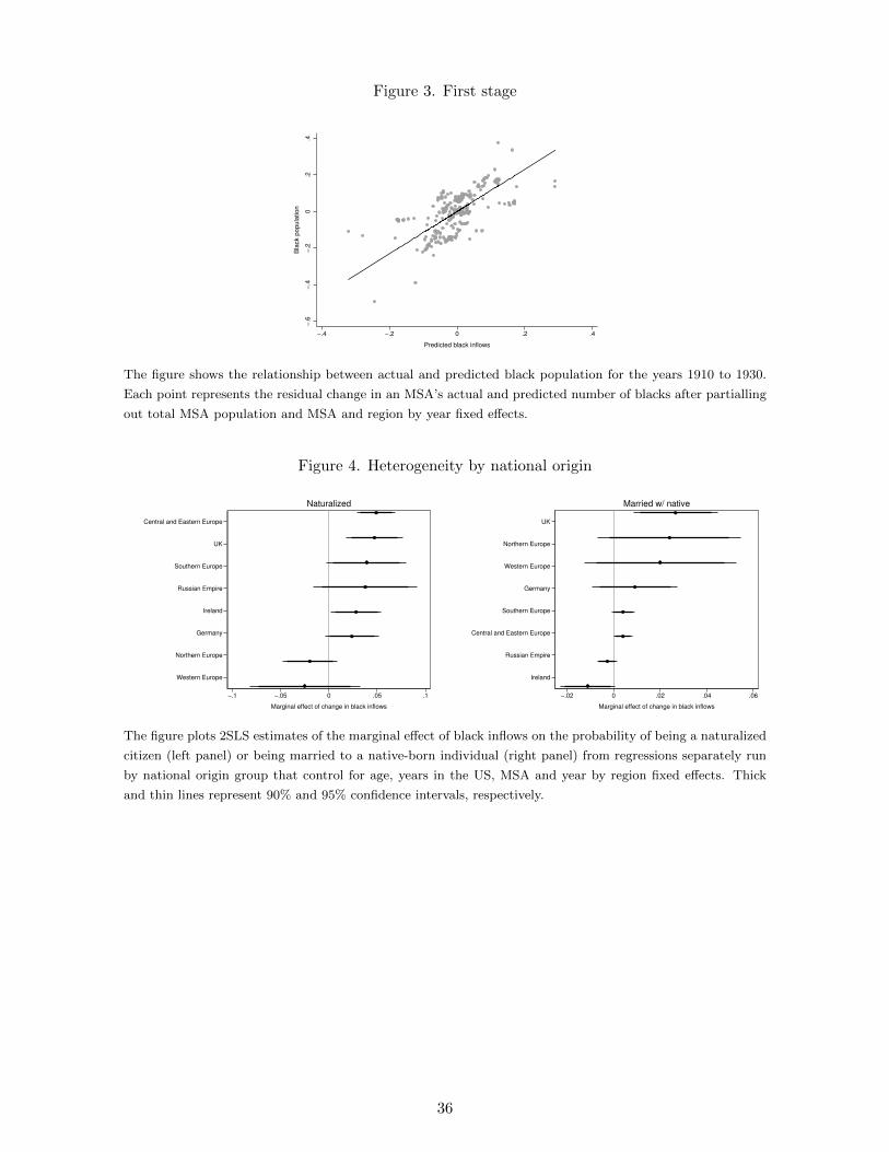
Figure 3. First stage

−.6

−.4

−.2

0.2

.4

Bla

ck p

op

ula

tio

n

−.4 −.2 0 .2 .4

Predicted black inflows

The figure shows the relationship between actual and predicted black population for the years 1910 to 1930.

Each point represents the residual change in an MSA’s actual and predicted number of blacks after partialling

out total MSA population and MSA and region by year fixed effects.

Figure 4. Heterogeneity by national origin

Central and Eastern Europe

UK

Southern Europe

Russian Empire

Ireland

Germany

Northern Europe

Western Europe

−.1 −.05 0 .05 .1

Marginal effect of change in black inflows

Naturalized

UK

Northern Europe

Western Europe

Germany

Southern Europe

Central and Eastern Europe

Russian Empire

Ireland

−.02 0 .02 .04 .06

Marginal effect of change in black inflows

Married w/ native

The figure plots 2SLS estimates of the marginal effect of black inflows on the probability of being a naturalized

citizen (left panel) or being married to a native-born individual (right panel) from regressions separately run

by national origin group that control for age, years in the US, MSA and year by region fixed effects. Thick

and thin lines represent 90% and 95% confidence intervals, respectively.

36

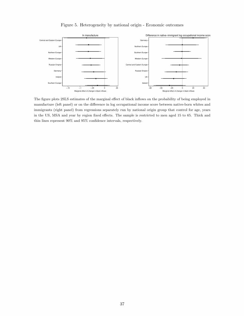
Figure 5. Heterogeneity by national origin - Economic outcomes

Central and Eastern Europe

UK

Northern Europe

Western Europe

Russian Empire

Germany

Ireland

Southern Europe

−.15 −.1 −.05 0 .05

Marginal effect of change in black inflows

In manufacture

Germany

Northern Europe

Southern Europe

Western Europe

Central and Eastern Europe

Russian Empire

UK

Ireland

−60 −40 −20 0 20 40

Marginal effect of change in black inflows

Difference in native−immigrant log occupational income score

The figure plots 2SLS estimates of the marginal effect of black inflows on the probability of being employed in

manufacture (left panel) or on the difference in log occupational income score between native-born whites and

immigrants (right panel) from regressions separately run by national origin group that control for age, years

in the US, MSA and year by region fixed effects. The sample is restricted to men aged 15 to 65. Thick and

thin lines represent 90% and 95% confidence intervals, respectively.

37

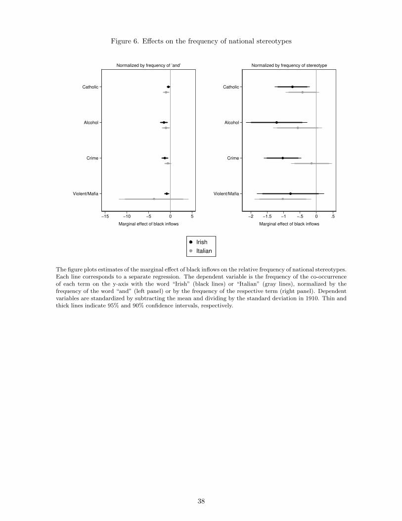
Figure 6. Effects on the frequency of national stereotypes

Catholic

Alcohol

Crime

Violent/Mafia

−15 −10 −5 0 5

Marginal effect of black inflows

Normalized by frequency of ’and’

Catholic

Alcohol

Crime

Violent/Mafia

−2 −1.5 −1 −.5 0 .5

Marginal effect of black inflows

Normalized by frequency of stereotype

Irish

Italian

The figure plots estimates of the marginal effect of black inflows on the relative frequency of national stereotypes.Each line corresponds to a separate regression. The dependent variable is the frequency of the co-occurrenceof each term on the y-axis with the word “Irish” (black lines) or “Italian” (gray lines), normalized by thefrequency of the word “and” (left panel) or by the frequency of the respective term (right panel). Dependentvariables are standardized by subtracting the mean and dividing by the standard deviation in 1910. Thin andthick lines indicate 95% and 90% confidence intervals, respectively.

38

Figure 7. Heterogeneity by distance from native-born whites

0.0

05

.01

.015

.02

.025

Marg

inal effect of bla

ck inflow

s o

n p

robabili

ty o

f bein

g m

arr

ied w

/ native

0 200 400 600 800 1000

Genetic distance

0.0

2.0

4.0

6.0

8

Marg

inal effect of bla

ck inflow

s o

n p

robabili

ty o

f natu

raliz

ation

0 200 400 600 800 1000

Genetic distance

0.0

05

.01

.015

.02

.025

Marg

inal effect of bla

ck inflow

s o

n p

robabili

ty o

f bein

g m

arr

ied w

/ native

0 1 2 3

Linguistic distance

0.0

2.0

4.0

6.0

8

Marg

inal effect of bla

ck inflow

s o

n p

robabili

ty o

f natu

raliz

ation

0 1 2 3

Linguistic distance

The figure plots the marginal effect of black inflows on the probability of being married with a native-born

individual (upper panel) and the probability of being a US citizen (lower panel) against values of genetic (left)

and linguistic distance (right). The underlying regressions are reported in Table 6.

39

Table 1. Summary statistics

Variables Mean Median S.D. Min Max N

MSA characteristics

MSA population 420,640 159,581 992,887 23,606 10,900,000 324

Number of immigrants 94,648 21,478 308,618 781 3,338,862 324

Number of blacks 15,294 2,349 44,830 29 485,750 324

Predicted number of blacks 3,350 328 13,308 -14,096 153,907 324

Share foreign-born 0.163 0.161 0.091 0.009 0.457 324

Share blacks 0.029 0.013 0.039 0.001 0.293 324

Main outcome variables

Married with native 0.150 0.132 0.085 0.036 0.498 324

Share naturalized 0.568 0.569 0.141 0.125 0.916 324

Notes: The sample consists of the 108 non-southern MSAs for which the instrument could be constructed,and is restricted to census years 1910, 1920, and 1930. Married with native refers to the share of immigrantmen who are married with a native-born spouse of native-born parentage. Share naturalized refers to the shareof immigrant men who are US citizens.

40

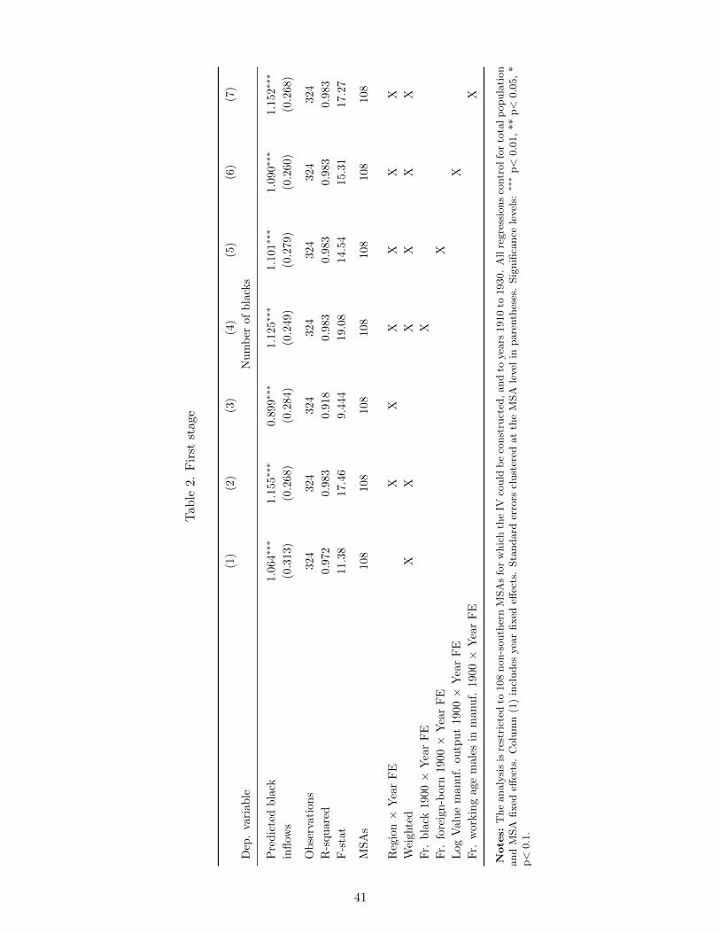
Tab

le2.

Fir

stst

age

(1)

(2)

(3)

(4)

(5)

(6)

(7)

Dep

.va

riab

leN

um

ber

of

bla

cks

Pre

dic

ted

bla

ck1.0

64∗

∗∗1.1

55∗

∗∗0.8

99∗∗

∗1.1

25∗

∗∗1.1

01∗∗

∗1.0

90∗

∗∗1.1

52∗∗

∗

infl

ows

(0.3

13)

(0.2

68)

(0.2

84)

(0.2

49)

(0.2

79)

(0.2

60)

(0.2

68)

Ob

serv

atio

ns

324

324

324

324

324

324

324

R-s

qu

ared

0.9

72

0.9

83

0.9

18

0.9

83

0.9

83

0.9

83

0.9

83

F-s

tat

11.3

817.4

69.4

44

19.0

814.5

415.3

117.2

7

MS

As

108

108

108

108

108

108

108

Reg

ion×

Yea

rF

EX

XX

XX

X

Wei

ghte

dX

XX

XX

X

Fr.

bla

ck19

00×

Yea

rF

EX

Fr.

fore

ign

-bor

n19

00×

Yea

rF

EX

Log

Val

ue

man

uf.

outp

ut

1900×

Yea

rF

EX

Fr.

wor

kin

gag

em

ales

inm

anu

f.19

00×

Yea

rF

EX

Note

s:T

he

analy

sis

isre

stri

cted

to108

non-s

outh

ern

MSA

sfo

rw

hic

hth

eIV

could

be

const

ruct

ed,

and

toyea

rs1910

to1930.

All

regre

ssio

ns

contr

olfo

rto

talp

opula

tion

and

MSA

fixed

effec

ts.

Colu

mn

(1)

incl

udes

yea

rfixed

effec

ts.

Sta

ndard

erro

rscl

ust

ered

at

the

MSA

level

inpare

nth

eses

.Sig

nifi

cance

level

s:∗∗∗

p<

0.0

1,

**

p<

0.0

5,

*p<

0.1

.

41

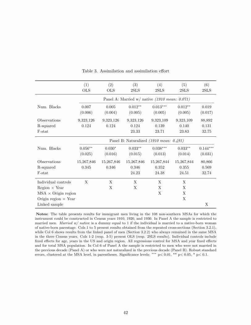
Table 3. Assimilation and assimilation effort

(1) (2) (3) (4) (5) (6)

OLS OLS 2SLS 2SLS 2SLS 2SLS

Panel A: Married w/ native (1910 mean: 0.071)

Num. Blacks 0.007 0.005 0.012∗∗ 0.013∗∗∗ 0.012∗∗ 0.019

(0.006) (0.004) (0.005) (0.005) (0.005) (0.017)

Observations 9,323,126 9,323,126 9,323,126 9,323,109 9,323,109 88,892

R-squared 0.124 0.124 0.124 0.139 0.140 0.131

F-stat 23.33 23.71 23.83 32.75

Panel B: Naturalized (1910 mean: 0.491)

Num. Blacks 0.056∗∗ 0.030∗ 0.033∗∗ 0.038∗∗∗ 0.033∗∗ 0.144∗∗∗

(0.025) (0.016) (0.015) (0.013) (0.014) (0.031)

Observations 15,267,846 15,267,846 15,267,846 15,267,844 15,267,844 80,866

R-squared 0.345 0.346 0.346 0.352 0.355 0.569

F-stat 24.23 24.38 24.51 32.74

Individual controls X X X X X

Region × Year X X X X

MSA × Origin region X X

Origin region × Year X

Linked sample X

Notes: The table presents results for immigrant men living in the 108 non-southern MSAs for which theinstrument could be constructed in Census years 1910, 1920, and 1930. In Panel A the sample is restricted tomarried men. Married w/ native is a dummy equal to 1 if the individual is married to a native-born womanof native-born parentage. Cols 1 to 5 present results obtained from the repeated cross-sections (Section 3.2.1),while Col 6 shows results from the linked panel of men (Section 3.2.2) who always remained in the same MSAin the three Census years. Cols 1-2 (resp. 3-5) present OLS (resp. 2SLS results). Individual controls includefixed effects for age, years in the US and origin region. All regressions control for MSA and year fixed effectsand for total MSA population. In Col 6 of Panel A the sample is restricted to men who were not married inthe previous decade (Panel A) or who were not naturalized in the previous decade (Panel B). Robust standarderrors, clustered at the MSA level, in parentheses. Significance levels: ∗∗∗ p< 0.01, ** p< 0.05, * p< 0.1.

42

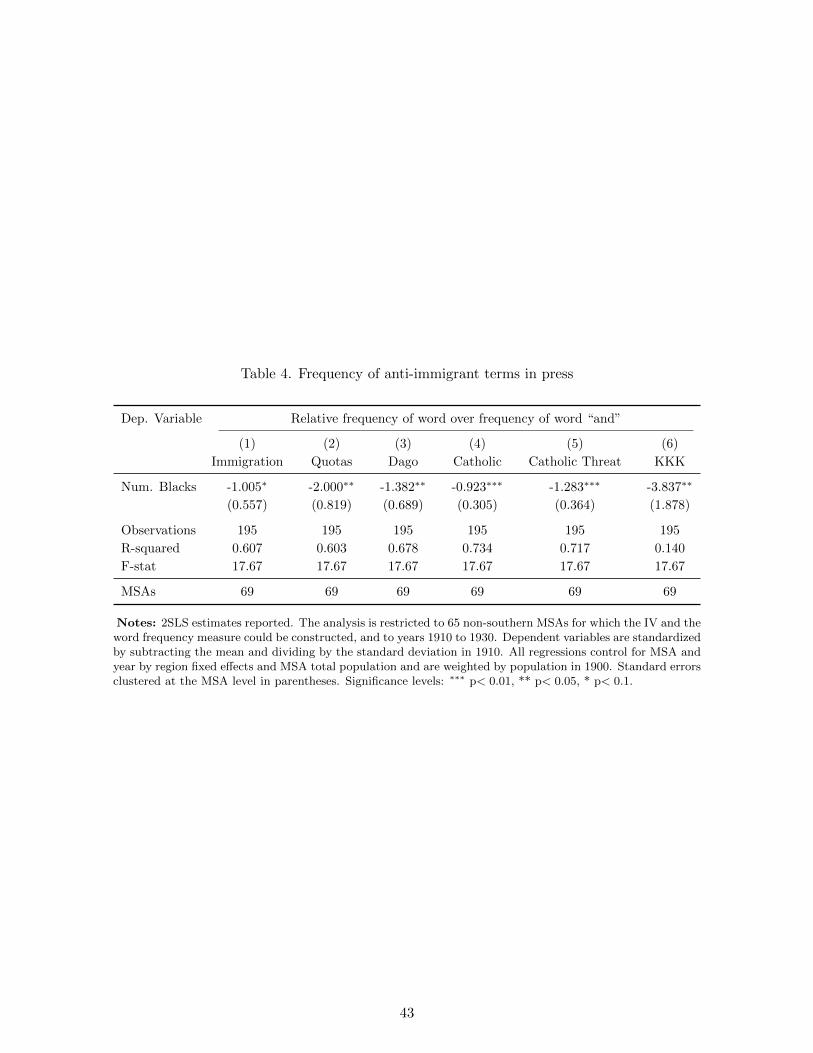
Table 4. Frequency of anti-immigrant terms in press

Dep. Variable Relative frequency of word over frequency of word “and”

(1) (2) (3) (4) (5) (6)

Immigration Quotas Dago Catholic Catholic Threat KKK

Num. Blacks -1.005∗ -2.000∗∗ -1.382∗∗ -0.923∗∗∗ -1.283∗∗∗ -3.837∗∗

(0.557) (0.819) (0.689) (0.305) (0.364) (1.878)

Observations 195 195 195 195 195 195

R-squared 0.607 0.603 0.678 0.734 0.717 0.140

F-stat 17.67 17.67 17.67 17.67 17.67 17.67

MSAs 69 69 69 69 69 69

Notes: 2SLS estimates reported. The analysis is restricted to 65 non-southern MSAs for which the IV and theword frequency measure could be constructed, and to years 1910 to 1930. Dependent variables are standardizedby subtracting the mean and dividing by the standard deviation in 1910. All regressions control for MSA andyear by region fixed effects and MSA total population and are weighted by population in 1900. Standard errorsclustered at the MSA level in parentheses. Significance levels: ∗∗∗ p< 0.01, ** p< 0.05, * p< 0.1.

43

Tab

le5.

Het

erog

enei

tyby

sect

orof

emp

loym

ent

and

skil

lin

1900

(1)

(2)

(3)

(4)

Dep

.va

riab

leM

arr

ied

w/

nati

veN

atu

ralize

dM

arri

edw

/nati

ve

Natu

ralize

d

Num

.bla

cks

0.01

1∗-0

.005

0.00

6-0

.005

(0.0

06)

(0.0

18)

(0.0

07)

(0.0

17)

Num

.bla

cks×

Shar

ein

man

ufa

cture

in190

00.0

040.1

35∗

∗∗

(0.0

09)

(0.0

18)

Num

.bla

cks×

Shar

eunsk

ille

din

1900

0.0

12

0.080∗

∗∗

(0.0

08)

(0.0

19)

Obse

rvat

ions

9,32

2,784

15,2

66,3

949,

322

,784

15,2

66,3

94

R-s

quar

ed0.

140

0.35

50.

140

0.3

55

F-s

tat

12.

3212.

5711.

95

12.2

9

Note

s:2SL

Ses

tim

ate

sre

port

ed.

The

analy

sis

isre

stri

cted

to108

non-s

outh

ern

MSA

sfo

rw

hic

hth

eIV

could

be

const

ruct

ed,

and

toyea

rs1910

to1930.

The

sam

ple

isre

stri

cted

tofo

reig

n-b

orn

men

InC

olu

mns

1and

3it

isfu

rther

rest

rict

edto

marr

ied

indiv

iduals

.A

llre

gre

ssio

ns

contr

ol

for

MSA

by

ori

gin

regio

n,

ori

gin

regio

nby

MSA

and

yea

rby

regio

nfixed

effec

tsand

MSA

tota

lp

opula

tion.

Sta

ndard

erro

rscl

ust

ered

at

the

MSA

level

inpare

nth

eses

.Sig

nifi

cance

level

s:∗∗∗

p<

0.0

1,

**

p<

0.0

5,

*p<

0.1

.

44

Tab

le6.

Het

erog

enei

tyby

dis

tan

cefr

omn

ativ

e-b

orn

wh

ites

(1)

(2)

(3)

(4)

Dep

.va

riab

leM

arri

edw

/nat

ive

Nat

ura

lize

dM

arr

ied

w/

nat

ive

Natu

ralize

d

Num

.bla

cks

0.01

1∗∗

0.02

9∗∗

0.01

1∗∗

0.0

21

(0.0

04)

(0.0

14)

(0.0

05)

(0.0

15)

Num

.bla

cks×

Gen

etic

dis

tance

0.000

∗∗0.

000

∗∗∗

(0.0

00)

(0.0

00)

Num

.bla

cks×

Gen

etic

dis

tance

2-0

.000∗∗

-0.0

00∗∗

∗

(0.0

00)

(0.0

00)

Num

.bla

cks×

Lin

guis

tic

dis

tance

-0.0

010.

041∗

∗∗

(0.0

02)

(0.0

06)

Num

.bla

cks×

Lin

guis

tic

dis

tance

20.

001

-0.0

14∗∗

∗

(0.0

01)

(0.0

02)

Obse

rvat

ions

9,22

0,6

6414,

978,

414

9,219

,280

15,0

12,4

24

R-s

quar

ed0.

144

0.35

80.

145

0.3

58

F-s

tat

8.14

58.

371

7.96

98.2

11

Note

s:2SL

Ses

tim

ate

sre

port

ed.

The

analy

sis

isre

stri

cted

to108

non-s

outh

ern

MSA

sfo

rw

hic

hth

eIV

could

be

const

ruct

ed,

and

toyea

rs1910

to1930.

The

sam

ple

isre

stri

cted

tofo

reig

n-b

orn

men

InC

olu

mns

1and

3it

isfu

rther

rest

rict

edto

marr

ied

indiv

iduals

.A

llre

gre

ssio

ns

incl

ude

fixed

effec

tsfo

rage,

yea

rsin

the

US,

MSA

by

nati

onality

,nati

onality

by

yea

rand

yea

rby

regio

n,

and

contr

ol

for

MSA

tota

lp

opula

tion.

Sta

ndard

erro

rscl

ust

ered

at

the

MSA

level

inpare

nth

eses

.Sig

nifi

cance

level

s:∗∗∗

p<

0.0

1,

**

p<

0.0

5,

*p<

0.1

.

45

Appendix (Not for publication)

Table of Contents

A Additional Figures and Tables 47

B Data Appendix 57

B.1 Foreign name index . . . . . . . . . . . . . . . . . . . . . . . . . . . . . . . . 57

B.2 Linked sample construction . . . . . . . . . . . . . . . . . . . . . . . . . . . 57

B.3 Push instrument . . . . . . . . . . . . . . . . . . . . . . . . . . . . . . . . . 60

C Robustness Checks 62

D Additional outcomes 75

D.1 Additional Economic and Social Outcomes . . . . . . . . . . . . . . . . . . . 75

D.2 Residential Segregation . . . . . . . . . . . . . . . . . . . . . . . . . . . . . 78

E A simple theoretical framework 81

E.1 Basic model . . . . . . . . . . . . . . . . . . . . . . . . . . . . . . . . . . . . 81

E.2 Stochastic extension . . . . . . . . . . . . . . . . . . . . . . . . . . . . . . . 86

46

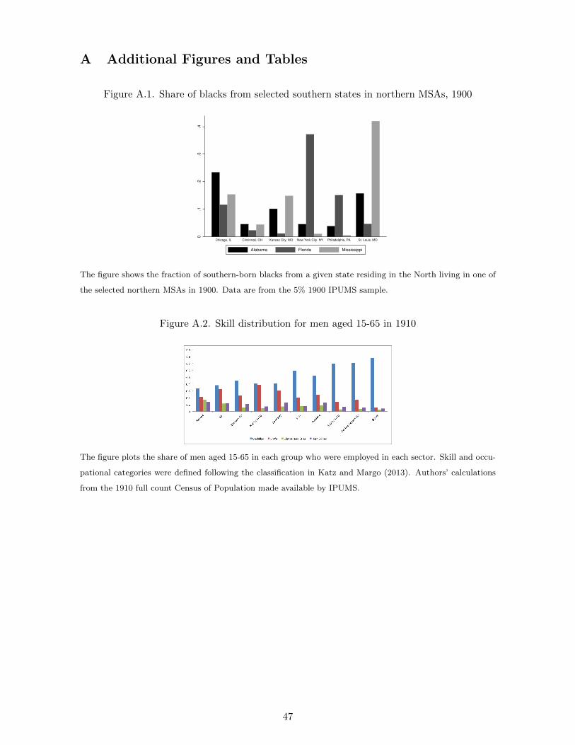
A Additional Figures and Tables

Figure A.1. Share of blacks from selected southern states in northern MSAs, 1900

0.1

.2.3

.4

Chicago, IL Cincinnati, OH Kansas City, MO New York City. NY Philadelphia, PA St. Louis, MO

Alabama Florida Mississippi

The figure shows the fraction of southern-born blacks from a given state residing in the North living in one of

the selected northern MSAs in 1900. Data are from the 5% 1900 IPUMS sample.

Figure A.2. Skill distribution for men aged 15-65 in 1910

The figure plots the share of men aged 15-65 in each group who were employed in each sector. Skill and occu-

pational categories were defined following the classification in Katz and Margo (2013). Authors’ calculations

from the 1910 full count Census of Population made available by IPUMS.

47

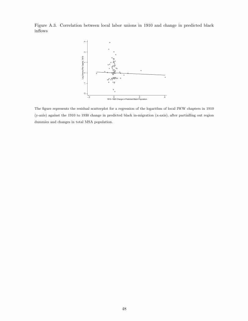
Figure A.3. Correlation between local labor unions in 1910 and change in predicted blackinflows

−2

−1

01

23

Lo

g U

nio

ns P

er

Ca

pita

, 1

91

0

−.2 0 .2 .41910−1920 Change in Predicted Black Population

The figure represents the residual scatterplot for a regression of the logarithm of local IWW chapters in 1910

(y-axis) against the 1910 to 1930 change in predicted black in-migration (x-axis), after partialling out region

dummies and changes in total MSA population.

48

Table A.1. List of MSAs

Akron, OH Flint, MI New York, NY Scranton, PA

Albany-Schenectady-Troy, NY Fort Wayne, IN Omaha, NE/IA Wilkes-Barre-Hazleton, PA

Albuquerque, NM Fresno, CA Peoria, IL Seattle-Everett, WA

Allentown-Bethlehem- Easton, PA Grand Rapids, MI Philadelphia, PA/NJ Sioux City, IA/NE

Altoona, PA Green Bay, WI Phoenix-Mesa, AZ Sioux Falls, SD

Atlantic City, NJ Hamilton-Middletown, OH Pittsburgh, PA South Bend, IN

Baltimore, MD Harrisburg-Leban-Carlisle, PA Pittsfield, MA Spokane, WA

Binghamton, NY Hartford, CT Portland, ME Springfield, IL

Boston, MA Huntington, WV/KY/OH Portland-Vancouver, OR/WA Springfield, MO

Bridgeport, CT Indianapolis, IN Providence, RI Springfield-Holyoke, MA

Brockton, MA Jackson, MI Fall River, MA/RI Springfield, OH

Buffalo, NY Johnstown, PA Pueblo, CO Stockton, CA

Canton, OH Kalamazoo, MI Racine, WI Syracuse, NY

Cedar Rapids, IA Kansas City, MO/KS Reading, PA Tacoma, WA

Chicago, IL Kenosha, WI San Bernardino, CA Terre Haute, IN

Cincinatti-Hamilton, OH/KY/IN Lancaster, PA Rochester, NY Toledo, OH/MI

Cleveland, OH Lansing-East Lansing, MI Rockford, IL Topeka, KS

Columbus, OH Lima, OH Sacramento, CA Trenton, NJ

Davenport-Moline-Rock Island, IA/IL Lincoln, NE Saginaw-Bay City-Midland, MI Utica-Rome, NY

Dayton, OH Lorain-Elyria, OH Bay City, MI Washington DC, MD/VA/WV

Decatur, IL Los Angeles-Long Beach, CA St. Joseph, MO Waterloo-Cedar Falls, IA

Denver, CO Louisville, KY/IN St. Louis, MO/IL Wheeling, WV/OH

Des Moines, IA Manchester, NH Salt Lake City, UT Wichita, KS

Detroit, MI Milwaukee-Waukesha, WI Ogden, UT Wilmington, DE/NJ/MD

Duluth-Superior, MN/WI Minneapolis-St. Paul, MN San Diego, CA Worcester, MA

Erie, PA Muncie, IN San Francisco, CA York, PA

Evansville, IN/KY New Haven-Meriden, CT San Jose, CA Youngstown-Warren, OH

49

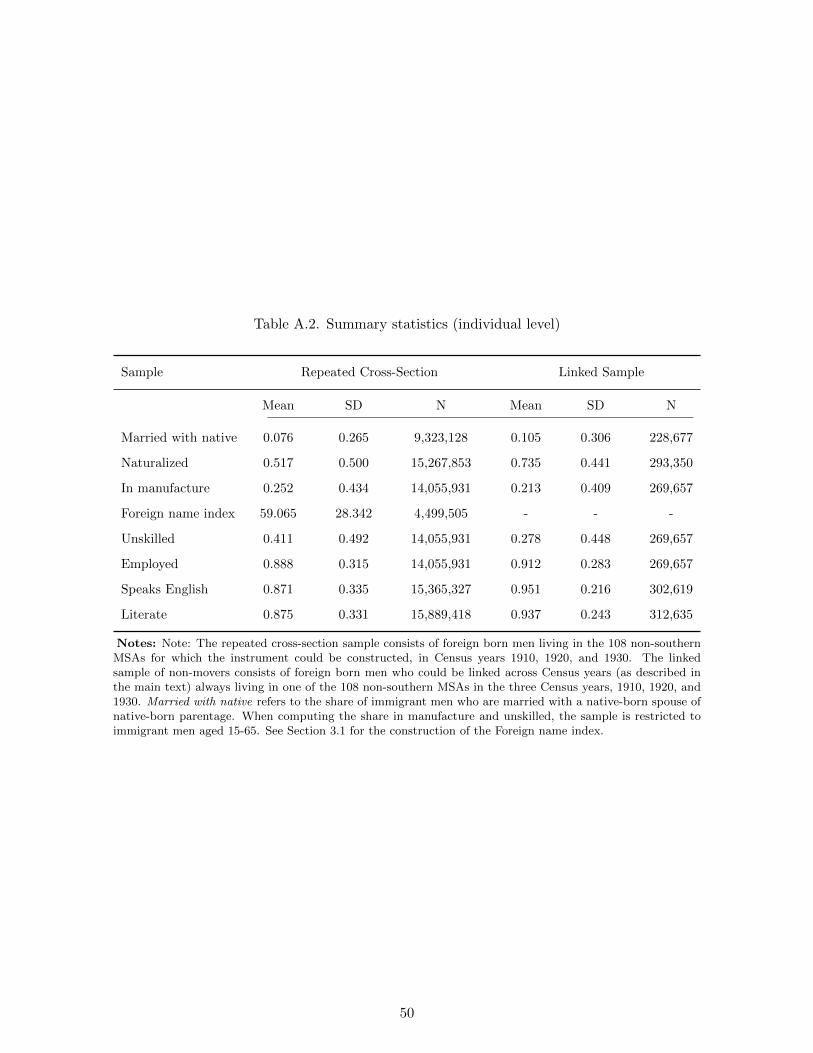
Table A.2. Summary statistics (individual level)

Sample Repeated Cross-Section Linked Sample

Mean SD N Mean SD N

Married with native 0.076 0.265 9,323,128 0.105 0.306 228,677

Naturalized 0.517 0.500 15,267,853 0.735 0.441 293,350

In manufacture 0.252 0.434 14,055,931 0.213 0.409 269,657

Foreign name index 59.065 28.342 4,499,505 - - -

Unskilled 0.411 0.492 14,055,931 0.278 0.448 269,657

Employed 0.888 0.315 14,055,931 0.912 0.283 269,657

Speaks English 0.871 0.335 15,365,327 0.951 0.216 302,619

Literate 0.875 0.331 15,889,418 0.937 0.243 312,635

Notes: Note: The repeated cross-section sample consists of foreign born men living in the 108 non-southernMSAs for which the instrument could be constructed, in Census years 1910, 1920, and 1930. The linkedsample of non-movers consists of foreign born men who could be linked across Census years (as described inthe main text) always living in one of the 108 non-southern MSAs in the three Census years, 1910, 1920, and1930. Married with native refers to the share of immigrant men who are married with a native-born spouse ofnative-born parentage. When computing the share in manufacture and unskilled, the sample is restricted toimmigrant men aged 15-65. See Section 3.1 for the construction of the Foreign name index.

50

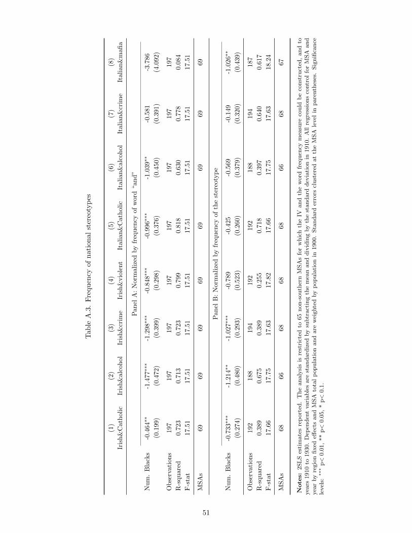
Tab

leA

.3.

Fre

qu

ency

ofn

atio

nal

ster

eoty

pes

(1)

(2)

(3)

(4)

(5)

(6)

(7)

(8)

Iris

h&

Cat

hol

icIr

ish

&al

coh

olIr

ish

&cr

ime

Iris

h&

vio

lent

Itali

an

&C

ath

oli

cIt

ali

an

&alc

oh

ol

Itali

an&

crim

eIt

alian

&m

afi

a

Pan

elA

:N

orm

ali

zed

by

freq

uen

cyof

word

“an

d”

Nu

m.

Bla

cks

-0.4

64∗∗

-1.4

77∗∗

∗-1

.298∗∗

∗-0

.848∗

∗∗-0

.996∗∗

∗-1

.039∗∗

-0.5

81

-3.7

86

(0.1

99)

(0.4

72)

(0.3

99)

(0.2

98)

(0.3

76)

(0.4

50)

(0.3

91)

(4.0

92)

Ob

serv

atio

ns

197

197

197

197

197

197

197

197

R-s

qu

ared

0.72

30.

713

0.7

23

0.7

99

0.8

18

0.6

30

0.7

78

0.0

84

F-s

tat

17.5

117

.51

17.5

117.5

117.5

117.5

117.5

117.5

1

MS

As

6969

69

69

69

69

69

69

Pan

elB

:N

orm

ali

zed

by

freq

uen

cyof

the

ster

eoty

pe

Nu

m.

Bla

cks

-0.7

33∗∗

∗-1

.214

∗∗-1

.027∗∗

∗-0

.789

-0.4

25

-0.5

69

-0.1

49

-1.0

26∗

∗

(0.2

74)

(0.4

80)

(0.2

93)

(0.5

23)

(0.2

60)

(0.3

79)

(0.3

20)

(0.4

39)

Ob

serv

atio

ns

192

188

194

192

192

188

194

187

R-s

qu

ared

0.38

90.

675

0.3

89

0.2

55

0.7

18

0.3

97

0.6

40

0.6

17

F-s

tat

17.6

617

.75

17.6

317.8

217.6

617.7

517.6

318.2

4

MS

As

6866

68

68

68

66

68

67

Note

s:2SL

Ses

tim

ate

sre

port

ed.

The

analy

sis

isre

stri

cted

to65

non-s

outh

ern

MSA

sfo

rw

hic

hth

eIV

and

the

word

freq

uen

cym

easu

reco

uld

be

const

ruct

ed,

and

toyea

rs1910

to1930.

Dep

enden

tva

riable

sare

standard

ized

by

subtr

act

ing

the

mea

nand

div

idin

gby

the

standard

dev

iati

on

in1910.

All

regre

ssio

ns

contr

ol

for

MSA

and

yea

rby

regio

nfixed

effec

tsand

MSA

tota

lp

opula

tion

and

are

wei

ghte

dby

popula

tion

in1900.

Sta

ndard

erro

rscl

ust

ered

at

the

MSA

level

inpare

nth

eses

.Sig

nifi

cance

level

s:∗∗∗

p<

0.0

1,

**

p<

0.0

5,

*p<

0.1

.

51

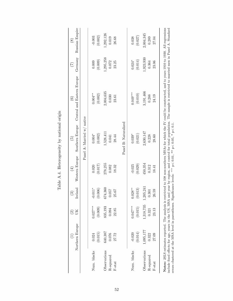
Tab

leA

.4.

Het

erog

enei

tyby

nat

ion

alor

igin

(1)

(2)

(3)

(4)

(5)

(6)

(7)

(8)

Nor

ther

nE

uro

pe

UK

Irel

and

Wes

tern

Euro

pe

South

ern

Euro

pe

Cen

tral

and

Eas

tern

Euro

pe

Ger

many

Russ

ian

Em

pir

e

Pan

elA

:M

arri

edw

/nat

ive

Num

.bla

cks

0.02

40.

027∗∗

∗-0

.011

∗0.

020

0.0

04∗

0.0

04∗∗

0.00

9-0

.003

(0.0

15)

(0.0

09)

(0.0

06)

(0.0

17)

(0.0

02)

(0.0

02)

(0.0

09)

(0.0

02)

Obse

rvati

ons

640,

387

835,

193

674

,360

278,

255

1,52

8,411

2,0

04,6

35

1,2

95,

258

1,2

92,1

26

R-s

quar

ed0.

076

0.09

40.0

57

0.0

820.0

410.0

300.

072

0.019

F-s

tat

27.7

222

.85

25.6

718.

3228

.44

23.6

123

.25

26.6

8

Pan

elB

:N

atura

lize

d

Num

.bla

cks

-0.0

200.

047∗∗

∗0.

028

∗∗-0

.025

0.039

∗0.

049∗

∗∗0.0

24∗

0.0

38

(0.0

14)

(0.0

15)

(0.0

13)

(0.0

29)

(0.0

21)

(0.0

10)

(0.0

14)

(0.0

27)

Obse

rvat

ions

1,09

5,17

71,

318,

735

1,2

05,2

41450

,354

2,6

30,1

47

3,19

1,4

661,

923

,930

2,00

4,345

R-s

quar

ed0.

322

0.32

10.3

010.

312

0.228

0.2

880.

364

0.28

9

F-s

tat

27.0

923.

1326

.59

18.4

128

.60

24.1

923.

06

27.0

4

Note

s:2S

LS

esti

mate

sre

port

ed.

Th

ean

aly

sis

isre

stri

cted

to108

non

-sou

ther

nM

SA

sfo

rw

hic

hth

eIV

cou

ldb

eco

nst

ruct

ed,

an

dto

yea

rs1910

to1930.

All

regre

ssio

ns

incl

ud

efi

xed

effec

tsfo

rage,

yea

rsin

the

US

,M

SA

an

dyea

rby

regio

n,

an

dco

ntr

ol

for

tota

lp

op

ula

tion

.T

he

sam

ple

isre

stri

cted

tom

arr

ied

men

inP

an

elA

.S

tan

dard

erro

rscl

ust

ered

at

the

MS

Ale

vel

inp

are

nth

eses

.S

ign

ifica

nce

level

s:∗∗∗

p<

0.0

1,

**

p<

0.0

5,

*p<

0.1

.

52

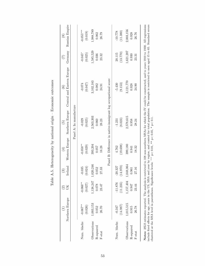
Tab

leA

.5.

Het

erog

enei

tyby

nat

ion

alor

igin

–E

con

omic

outc

omes

(1)

(2)

(3)

(4)

(5)

(6)

(7)

(8)

Nor

ther

nE

uro

pe

UK

Irel

and

Wes

tern

Euro

pe

South

ern

Euro

pe

Cen

tral

and

Eas

tern

Euro

pe

Ger

many

Russ

ian

Em

pir

e

Panel

A:

Inm

anufa

cture

Num

.bla

cks

-0.0

67∗∗

-0.0

66∗∗

-0.0

35

-0.0

58∗∗

-0.0

29-0

.074

-0.0

45∗

-0.0

55∗∗

∗

(0.0

26)

(0.0

27)

(0.0

24)

(0.0

29)

(0.0

25)

(0.0

47)

(0.0

25)

(0.0

19)

Obse

rvat

ions

1,00

3,15

31,

138,

247

1,02

0,2

46393

,204

2,5

63,3

03

3,10

2,183

1,58

5,5

291,

988,

789

R-s

quar

ed0.

052

0.0

780.

052

0.057

0.060

0.082

0.0

36

0.06

2

F-s

tat

26.7

023

.47

27.

3318

.28

28.2

324

.91

23.

3226.7

9

Pan

elB

:D

iffer

ence

innati

ve-

imm

igra

nt

log

occ

upat

ional

score

Num

.bla

cks

-0.3

47-1

1.87

6-2

0.3

274.7

62

-1.2

31-5

.430

20.1

15

-10.7

78

(14.

987)

(11.

235)

(14.

970

)(1

9.6

98)

(8.0

23)

(9.1

53)

(13.

770)

(11.

380)

Obse

rvat

ions

1,01

5,51

51,

157,

404

1,04

8,0

64399

,180

2,5

78,6

15

3,12

1,770

1,62

1,2

072,

003,

156

R-s

quar

ed0.

915

0.94

70.9

610.

941

0.95

80.

928

0.9

30

0.92

8

F-s

tat

26.7

823

.44

27.

1618

.32

28.2

424

.90

23.

3126.7

6

Note

s:2S

LS

esti

mate

sre

port

ed.

Th

ean

aly

sis

isre

stri

cted

to108

non

-sou

ther

nM

SA

sfo

rw

hic

hth

eIV

cou

ldb

eco

nst

ruct

ed,

an

dto

yea

rs1910

to1930.

All

regre

ssio

ns

incl

ud

efi

xed

effec

tsfo

rage,

yea

rsin

the

US

,M

SA

an

dyea

rby

regio

n,

an

dco

ntr

ol

for

tota

lp

op

ula

tion

.T

he

sam

ple

isre

stri

cted

tom

enaged

15

to65.

Sta

nd

ard

erro

rscl

ust

ered

at

the

MS

Ale

vel

inp

are

nth

eses

.S

ign

ifica

nce

level

s:∗∗∗

p<

0.0

1,

**

p<

0.0

5,

*p<

0.1

.

53

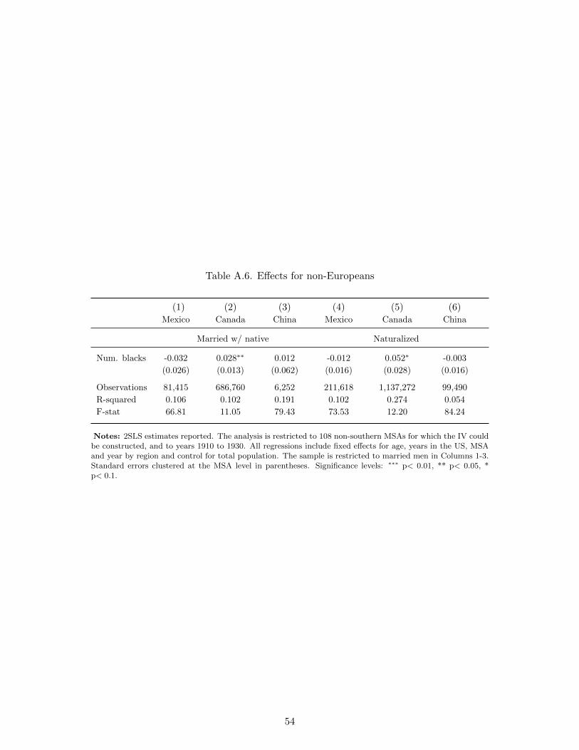
Table A.6. Effects for non-Europeans

(1) (2) (3) (4) (5) (6)Mexico Canada China Mexico Canada China

Married w/ native Naturalized

Num. blacks -0.032 0.028∗∗ 0.012 -0.012 0.052∗ -0.003

(0.026) (0.013) (0.062) (0.016) (0.028) (0.016)

Observations 81,415 686,760 6,252 211,618 1,137,272 99,490

R-squared 0.106 0.102 0.191 0.102 0.274 0.054

F-stat 66.81 11.05 79.43 73.53 12.20 84.24

Notes: 2SLS estimates reported. The analysis is restricted to 108 non-southern MSAs for which the IV couldbe constructed, and to years 1910 to 1930. All regressions include fixed effects for age, years in the US, MSAand year by region and control for total population. The sample is restricted to married men in Columns 1-3.Standard errors clustered at the MSA level in parentheses. Significance levels: ∗∗∗ p< 0.01, ** p< 0.05, *p< 0.1.

54

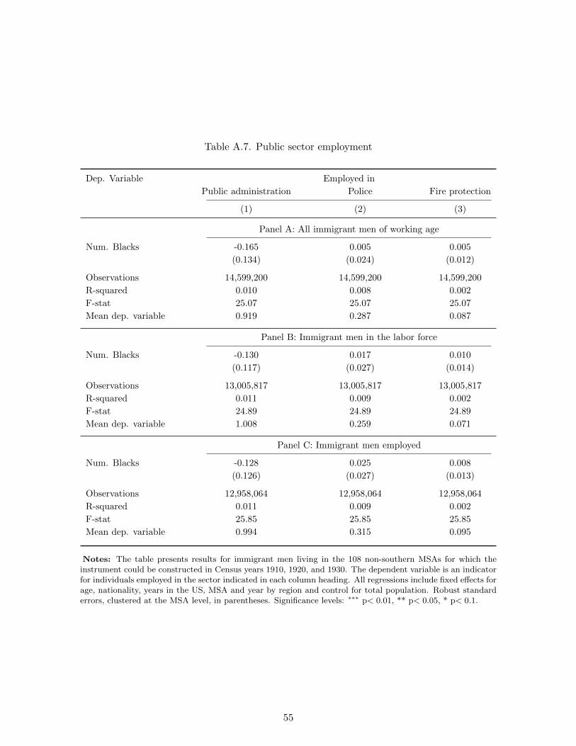
Table A.7. Public sector employment

Dep. Variable Employed in

Public administration Police Fire protection

(1) (2) (3)

Panel A: All immigrant men of working age

Num. Blacks -0.165 0.005 0.005

(0.134) (0.024) (0.012)

Observations 14,599,200 14,599,200 14,599,200

R-squared 0.010 0.008 0.002

F-stat 25.07 25.07 25.07

Mean dep. variable 0.919 0.287 0.087

Panel B: Immigrant men in the labor force

Num. Blacks -0.130 0.017 0.010

(0.117) (0.027) (0.014)

Observations 13,005,817 13,005,817 13,005,817

R-squared 0.011 0.009 0.002

F-stat 24.89 24.89 24.89

Mean dep. variable 1.008 0.259 0.071

Panel C: Immigrant men employed

Num. Blacks -0.128 0.025 0.008

(0.126) (0.027) (0.013)

Observations 12,958,064 12,958,064 12,958,064

R-squared 0.011 0.009 0.002

F-stat 25.85 25.85 25.85

Mean dep. variable 0.994 0.315 0.095

Notes: The table presents results for immigrant men living in the 108 non-southern MSAs for which theinstrument could be constructed in Census years 1910, 1920, and 1930. The dependent variable is an indicatorfor individuals employed in the sector indicated in each column heading. All regressions include fixed effects forage, nationality, years in the US, MSA and year by region and control for total population. Robust standarderrors, clustered at the MSA level, in parentheses. Significance levels: ∗∗∗ p< 0.01, ** p< 0.05, * p< 0.1.

55

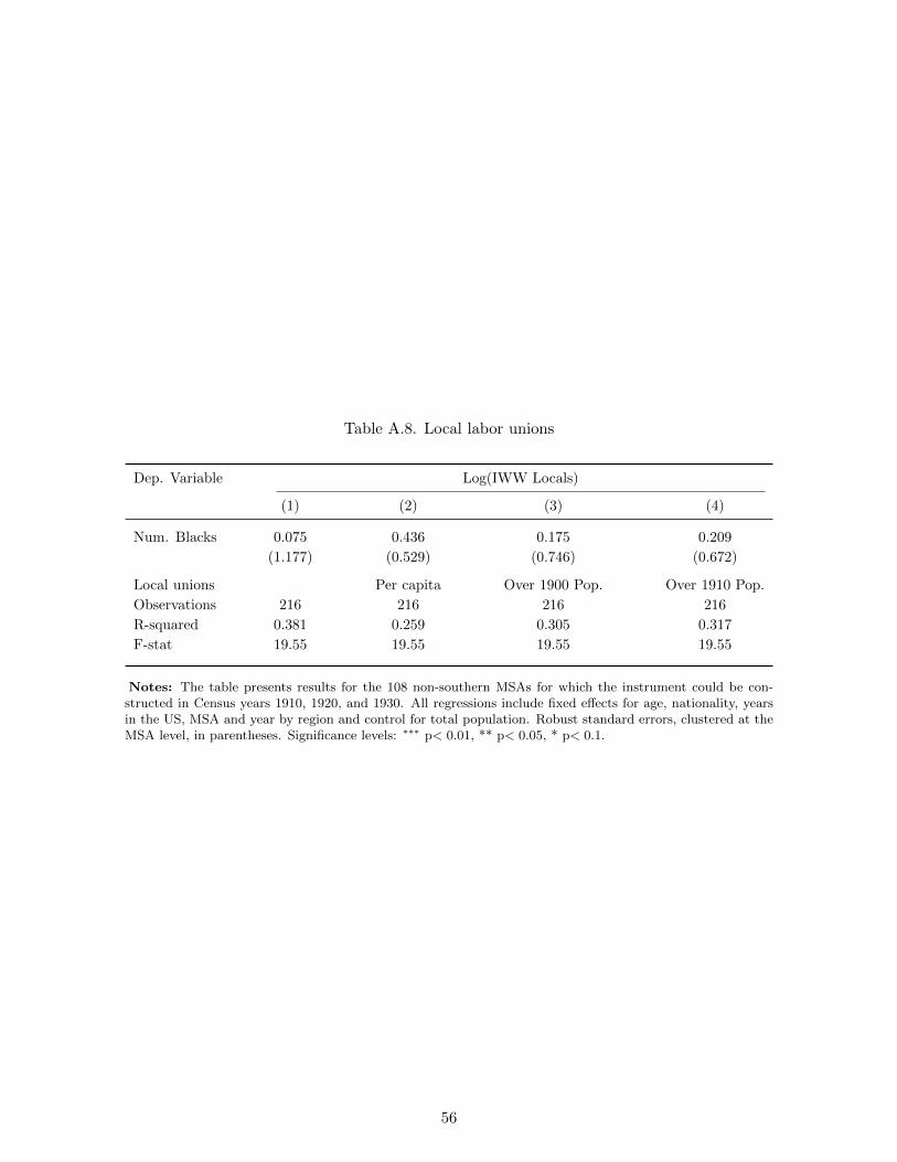
Table A.8. Local labor unions

Dep. Variable Log(IWW Locals)

(1) (2) (3) (4)

Num. Blacks 0.075 0.436 0.175 0.209

(1.177) (0.529) (0.746) (0.672)

Local unions Per capita Over 1900 Pop. Over 1910 Pop.

Observations 216 216 216 216

R-squared 0.381 0.259 0.305 0.317

F-stat 19.55 19.55 19.55 19.55

Notes: The table presents results for the 108 non-southern MSAs for which the instrument could be con-structed in Census years 1910, 1920, and 1930. All regressions include fixed effects for age, nationality, yearsin the US, MSA and year by region and control for total population. Robust standard errors, clustered at theMSA level, in parentheses. Significance levels: ∗∗∗ p< 0.01, ** p< 0.05, * p< 0.1.

56

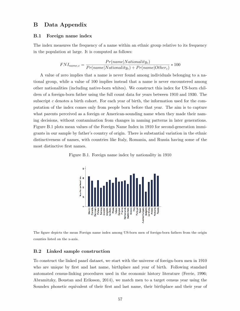
B Data Appendix

B.1 Foreign name index

The index measures the frequency of a name within an ethnic group relative to its frequency

in the population at large. It is computed as follows:

FNIname,c =Pr(name|Nationalityc)

Pr(name|Nationalityc) + Pr(name|Otherc)∗ 100

A value of zero implies that a name is never found among individuals belonging to a na-

tional group, while a value of 100 implies instead that a name is never encountered among

other nationalities (including native-born whites). We construct this index for US-born chil-

dren of a foreign-born father using the full count data for years between 1910 and 1930. The

subscript c denotes a birth cohort. For each year of birth, the information used for the com-

putation of the index comes only from people born before that year. The aim is to capture

what parents perceived as a foreign or American-sounding name when they made their nam-

ing decisions, without contamination from changes in naming patterns in later generations.

Figure B.1 plots mean values of the Foreign Name Index in 1910 for second-generation immi-

grants in our sample by father’s country of origin. There is substantial variation in the ethnic

distinctiveness of names, with countries like Italy, Romania, and Russia having some of the

most distinctive first names.

Figure B.1. Foreign name index by nationality in 1910

The figure depicts the mean Foreign name index among US-born men of foreign-born fathers from the origin

counties listed on the x-axis.

B.2 Linked sample construction

To construct the linked panel dataset, we start with the universe of foreign-born men in 1910

who are unique by first and last name, birthplace and year of birth. Following standard

automated census-linking procedures used in the economic history literature (Ferrie, 1996;

Abramitzky, Boustan and Eriksson, 2014), we match men to a target census year using the

Soundex phonetic equivalent of their first and last name, their birthplace and their year of

57

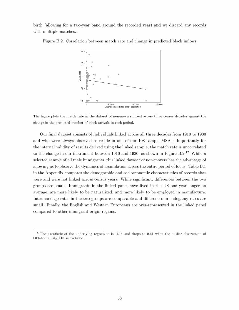
birth (allowing for a two-year band around the recorded year) and we discard any records

with multiple matches.

Figure B.2. Correlation between match rate and change in predicted black inflows

0.0

5.1

.15

.2M

atc

h r

ate

0 50000 100000 150000Change in predicted black population

The figure plots the match rate in the dataset of non-movers linked across three census decades against the

change in the predicted number of black arrivals in each period.

Our final dataset consists of individuals linked across all three decades from 1910 to 1930

and who were always observed to reside in one of our 108 sample MSAs. Importantly for

the internal validity of results derived using the linked sample, the match rate is uncorrelated

to the change in our instrument between 1910 and 1930, as shown in Figure B.2.17 While a

selected sample of all male immigrants, this linked dataset of non-movers has the advantage of

allowing us to observe the dynamics of assimilation across the entire period of focus. Table B.1

in the Appendix compares the demographic and socioeconomic characteristics of records that

were and were not linked across census years. While significant, differences between the two

groups are small. Immigrants in the linked panel have lived in the US one year longer on

average, are more likely to be naturalized, and more likely to be employed in manufacture.

Intermarriage rates in the two groups are comparable and differences in endogamy rates are

small. Finally, the English and Western Europeans are over-represented in the linked panel

compared to other immigrant origin regions.

17The t-statistic of the underlying regression is -1.14 and drops to 0.61 when the outlier observation ofOklahoma City, OK is excluded.

58

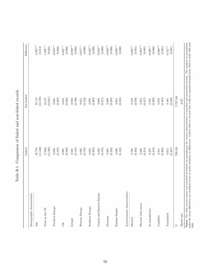
Tab

leB

.1.

Com

par

ison

ofli

nke

dan

dn

on-l

inke

dre

cord

s

Lin

ked

Not

-Lin

ked

Diff

eren

ce

Dem

ogra

phic

char

acte

rist

ics

Age

32.7

16

35.

113

-2.3

97∗∗

∗

(11.

440)

(12.

470)

(0.0

14)

Yea

rsin

the

US

17.6

8616

.177

1.50

9∗∗∗

(11.2

95)

(12.9

51)

(0.0

25)

Nor

ther

nE

uro

pe

0.03

90.

058

-0.0

19∗∗

∗

(0.1

95)

(0.2

35)

(0.0

00)

UK

0.0

670.

044

0.0

22∗∗

∗

(0.2

49)

(0.2

06)

(0.0

00)

Irel

and

0.0

210.

040

-0.0

20∗∗

∗

(0.1

42)

(0.1

96)

(0.0

00)

Wes

tern

Euro

pe

0.03

20.0

15

0.01

7∗∗∗

(0.1

76)

(0.1

23)

(0.0

00)

Sou

ther

nE

uro

pe

0.04

40.

076

-0.0

32∗∗

∗

(0.2

05)

(0.2

65)

(0.0

00)

Cen

tral

and

Eas

tern

Euro

pe

0.03

20.

080

-0.0

48∗∗

∗

(0.1

76)

(0.2

71)

(0.0

00)

Ger

man

y0.

065

0.08

8-0

.022

∗∗∗

(0.2

50)

(0.2

84)

(0.0

00)

Russ

ian

Em

pir

e0.0

360.

064

-0.0

28∗∗

∗

(0.1

85)

(0.2

45)

(0.0

00)

Soci

oec

onom

icch

arac

teri

stic

s

Mar

ried

0.5

860.

548

0.0

38∗∗

∗

(0.4

92)

(0.5

00)

(0.0

01)

Mar

ried

wit

hnat

ive

0.2

200.

224

-0.0

04∗∗

∗

(0.4

14)

(0.4

17)

(0.0

01)

Inm

anufa

cture

0.22

70.

191

0.0

36∗∗

∗

(0.4

19)

(0.3

93)

(0.0

00)

Unsk

ille

d0.3

110.3

79-0

.068

∗∗∗

(0.4

63)

(0.4

85)

(0.0

01)

Nat

ura

lize

d0.6

120.

491

0.1

21∗∗

∗

(0.4

87)

(0.5

00)

(0.0

01)

N799

,193

7,7

27,5

28

Mat

chra

te9.4

%

Note

s:T

he

tab

lere

port

sm

ean

san

dst

an

dard

dev

iati

on

s(i

np

are

nth

eses

)fo

rva

riou

sch

ara

cter

isti

csof

matc

hed

an

du

nm

atc

hed

reco

rds.

Th

enu

mb

ers

inp

are

nth

eses

un

der

the

mea

nd

iffer

ence

sare

stan

dard

erro

rson

poin

tes

tim

ate

sof

diff

eren

ces.

Linked

refe

rsto

reco

rds

that

cou

ldb

em

atc

hed

forw

ard

from

1910

tob

oth

1920

an

d1930.

59

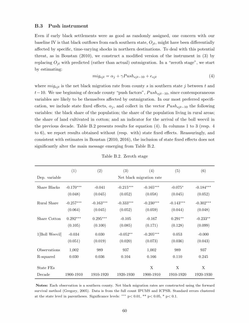
B.3 Push instrument

Even if early black settlements were as good as randomly assigned, one concern with our

baseline IV is that black outflows from each southern state, Ojt, might have been differentially

affected by specific, time-varying shocks in northern destinations. To deal with this potential

threat, as in Boustan (2010), we construct a modified version of the instrument in (3) by

replacing Ojt with predicted (rather than actual) outmigration. In a “zeroth stage”, we start

by estimating:

migsjt = αj + γPushsjt−10 + esjt (4)

where migsjt is the net black migration rate from county s in southern state j between t and

t−10. We use beginning of decade county “push factors”, Pushsjt−10, since contemporaneous

variables are likely to be themselves affected by outmigration. In our most preferred specifi-

cation, we include state fixed effects, αj , and collect in the vector Pushsjt−10 the following

variables: the black share of the population; the share of the population living in rural areas;

the share of land cultivated in cotton; and an indicator for the arrival of the boll weevil in

the previous decade. Table B.2 presents results for equation (4). In columns 1 to 3 (resp. 4

to 6), we report results obtained without (resp. with) state fixed effects. Reassuringly, and

consistent with estimates in Boustan (2010, 2016), the inclusion of state fixed effects does not

significantly alter the main message emerging from Table B.2.

Table B.2. Zeroth stage

(1) (2) (3) (4) (5) (6)

Dep. variable Net black migration rate

Share Blacks -0.170∗∗∗ -0.041 -0.215∗∗∗ -0.165∗∗∗ -0.075∗ -0.184∗∗∗

(0.048) (0.045) (0.052) (0.058) (0.045) (0.052)

Rural Share -0.257∗∗∗ -0.163∗∗∗ -0.333∗∗∗ -0.230∗∗∗ -0.143∗∗∗ -0.302∗∗∗

(0.064) (0.045) (0.052) (0.059) (0.044) (0.048)

Share Cotton 0.292∗∗∗ 0.295∗∗∗ -0.105 -0.167 0.291∗∗ -0.233∗∗

(0.105) (0.100) (0.085) (0.171) (0.128) (0.099)

1[Boll Weevil] -0.034 0.030 -0.052∗∗ -0.205∗∗∗ 0.053 -0.000

(0.051) (0.019) (0.020) (0.073) (0.036) (0.043)

Observations 1,002 989 937 1,002 989 937

R-squared 0.030 0.036 0.104 0.166 0.110 0.245

State FEs X X X

Decade 1900-1910 1910-1920 1920-1930 1900-1910 1910-1920 1920-1930

Notes: Each observation is a southern county. Net black migration rates are constructed using the forward

survival method (Gregory, 2005). Data is from the full count IPUMS and ICPSR. Standard errors clustered

at the state level in parentheses. Significance levels: ∗∗∗ p< 0.01, ** p< 0.05, * p< 0.1.

60

In line with the historical evidence (e.g. Boustan (2016)), a higher black share and a higher

fraction of the population living in rural areas are associated with larger black departures

during the subsequent decade. Also, counties with a larger share of land cultivated in cotton

were more likely to attract blacks between 1900 and 1920, but this pattern was reversed during

the 1920-1930 decade. Indeed, after 1920, cotton mechanization began to spread around the

South, reducing demand for black labor in agriculture and increasing incentives to migrate

northward (Wright, 1986). Finally, in line with findings in Collins and Wanamaker (2015), the

arrival of the boll weevil is significantly associated with black outflows only for the 1920-1930

decade.18

After estimating (4), we compute predicted migration flows from each county by multiply-

ing the fitted values from (4) with the county initial black population. Finally, we aggregate

these flows to the state level to obtain the predicted number of blacks leaving each southern

state j in each decade, Ojt. We then replace Ojt with Ojt in (3) to derive the (push-factors

induced) predicted number of blacks moving to city c in year t. By construction, this (pre-

dicted) measure of black outmigration from the South is orthogonal to any specific shock

occurring in the North. Moreover, by exploiting southern shocks to agricultural conditions,

this instrument is less likely to suffer from the problem of high serial correlation in migration

patterns between sending and receiving areas – a possible concern for standard shift-share in-

struments (Jaeger, Ruist and Stuhler, 2018). We show that both first stage and 2SLS results

are robust to using this, instead of our baseline version of the instrument.

18Results are very similar when including only a subset of the push factors used in (4), or when addingadditional controls such as the share of a county cultivated with tobacco, the presence of railroads, or averagefarm values.

61

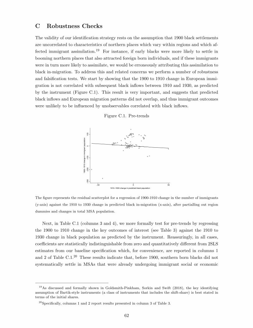
C Robustness Checks

The validity of our identification strategy rests on the assumption that 1900 black settlements

are uncorrelated to characteristics of northern places which vary within regions and which af-

fected immigrant assimilation.19 For instance, if early blacks were more likely to settle in

booming northern places that also attracted foreign born individuals, and if these immigrants

were in turn more likely to assimilate, we would be erroneously attributing this assimilation to

black in-migration. To address this and related concerns we perform a number of robustness

and falsification tests. We start by showing that the 1900 to 1910 change in European immi-

gration is not correlated with subsequent black inflows between 1910 and 1930, as predicted

by the instrument (Figure C.1). This result is very important, and suggests that predicted

black inflows and European migration patterns did not overlap, and thus immigrant outcomes

were unlikely to be influenced by unobservables correlated with black inflows.

Figure C.1. Pre-trends

−3

00

−2

00

−1

00

01

00

19

00

−1

91

0 c

ha

ng

e in

im

mig

ran

t p

op

ula

tio

n

−50 0 50

1910−1930 change in predicted black population

The figure represents the residual scatterplot for a regression of 1900-1910 change in the number of immigrants

(y-axis) against the 1910 to 1930 change in predicted black in-migration (x-axis), after partialling out region

dummies and changes in total MSA population.

Next, in Table C.1 (columns 3 and 4), we more formally test for pre-trends by regressing

the 1900 to 1910 change in the key outcomes of interest (see Table 3) against the 1910 to

1930 change in black population as predicted by the instrument. Reassuringly, in all cases,

coefficients are statistically indistinguishable from zero and quantitatively different from 2SLS

estimates from our baseline specification which, for convenience, are reported in columns 1

and 2 of Table C.1.20 These results indicate that, before 1900, southern born blacks did not

systematically settle in MSAs that were already undergoing immigrant social or economic

19As discussed and formally shown in Goldsmith-Pinkham, Sorkin and Swift (2018), the key identifyingassumption of Bartik-style instruments (a class of instruments that includes the shift-share) is best stated interms of the initial shares.

20Specifically, columns 1 and 2 report results presented in column 3 of Table 3.

62

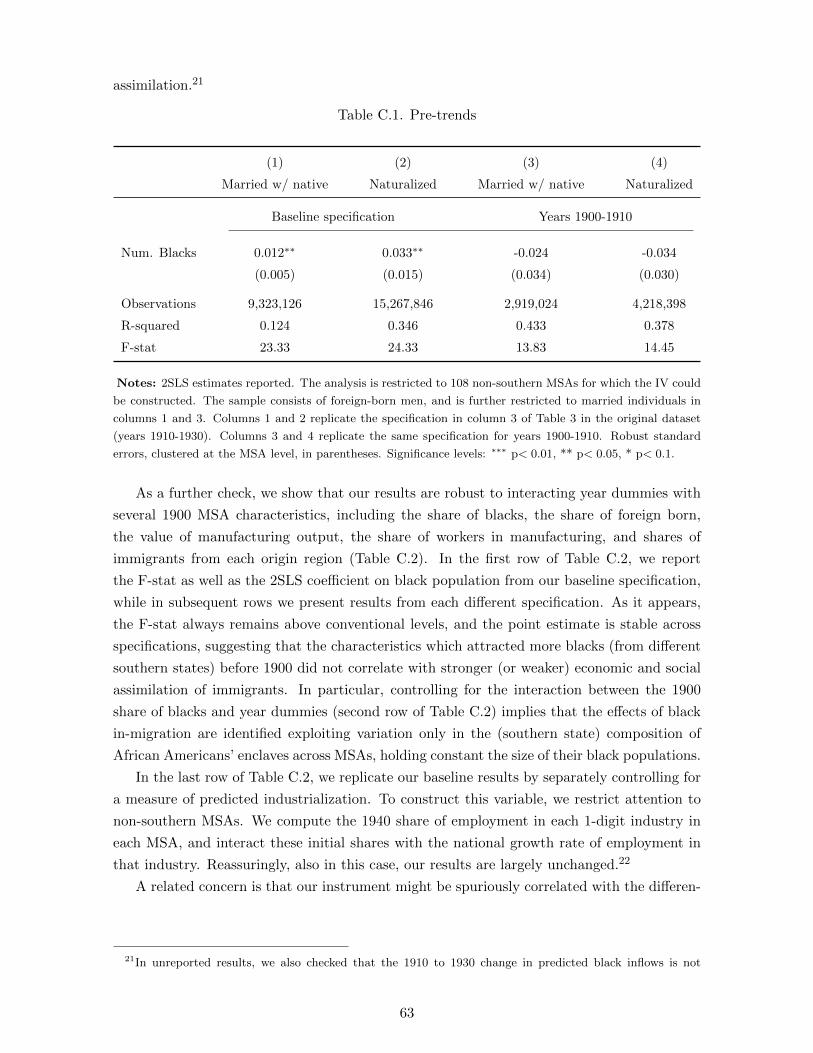
assimilation.21

Table C.1. Pre-trends

(1) (2) (3) (4)

Married w/ native Naturalized Married w/ native Naturalized

Baseline specification Years 1900-1910

Num. Blacks 0.012∗∗ 0.033∗∗ -0.024 -0.034

(0.005) (0.015) (0.034) (0.030)

Observations 9,323,126 15,267,846 2,919,024 4,218,398

R-squared 0.124 0.346 0.433 0.378

F-stat 23.33 24.33 13.83 14.45

Notes: 2SLS estimates reported. The analysis is restricted to 108 non-southern MSAs for which the IV could

be constructed. The sample consists of foreign-born men, and is further restricted to married individuals in

columns 1 and 3. Columns 1 and 2 replicate the specification in column 3 of Table 3 in the original dataset

(years 1910-1930). Columns 3 and 4 replicate the same specification for years 1900-1910. Robust standard

errors, clustered at the MSA level, in parentheses. Significance levels: ∗∗∗ p< 0.01, ** p< 0.05, * p< 0.1.

As a further check, we show that our results are robust to interacting year dummies with

several 1900 MSA characteristics, including the share of blacks, the share of foreign born,

the value of manufacturing output, the share of workers in manufacturing, and shares of

immigrants from each origin region (Table C.2). In the first row of Table C.2, we report

the F-stat as well as the 2SLS coefficient on black population from our baseline specification,

while in subsequent rows we present results from each different specification. As it appears,

the F-stat always remains above conventional levels, and the point estimate is stable across

specifications, suggesting that the characteristics which attracted more blacks (from different

southern states) before 1900 did not correlate with stronger (or weaker) economic and social

assimilation of immigrants. In particular, controlling for the interaction between the 1900

share of blacks and year dummies (second row of Table C.2) implies that the effects of black

in-migration are identified exploiting variation only in the (southern state) composition of

African Americans’ enclaves across MSAs, holding constant the size of their black populations.

In the last row of Table C.2, we replicate our baseline results by separately controlling for

a measure of predicted industrialization. To construct this variable, we restrict attention to

non-southern MSAs. We compute the 1940 share of employment in each 1-digit industry in

each MSA, and interact these initial shares with the national growth rate of employment in

that industry. Reassuringly, also in this case, our results are largely unchanged.22

A related concern is that our instrument might be spuriously correlated with the differen-

21In unreported results, we also checked that the 1910 to 1930 change in predicted black inflows is not

63

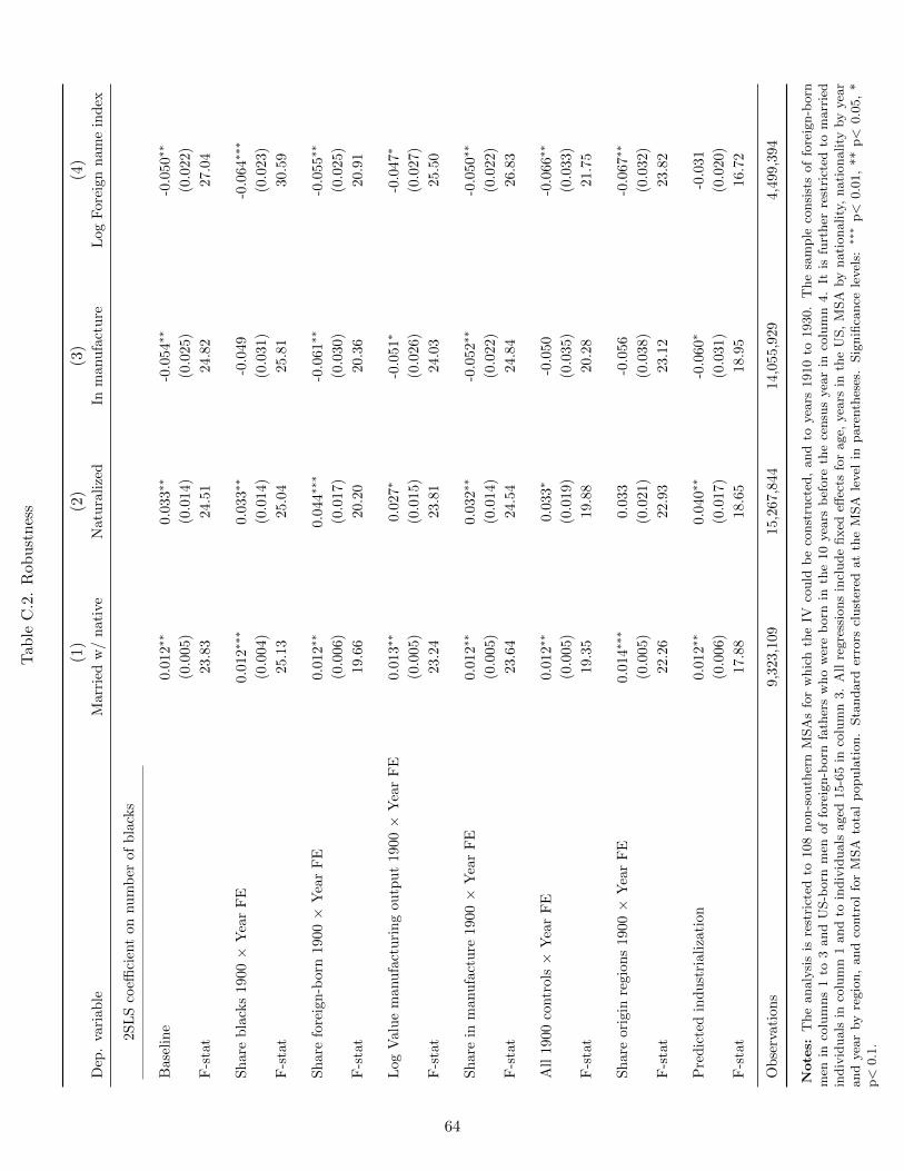
Tab

leC

.2.

Rob

ust

nes

s

(1)

(2)

(3)

(4)

Dep

.va

riab

leM

arr

ied

w/

nati

veN

atu

rali

zed

Inm

anu

fact

ure

Log

Fore

ign

nam

ein

dex

2SL

Sco

effici

ent

onnu

mb

erof

bla

cks

Bas

elin

e0.0

12∗

∗0.0

33∗∗

-0.0

54∗

∗-0

.050∗∗

(0.0

05)

(0.0

14)

(0.0

25)

(0.0

22)

F-s

tat

23.8

324.5

124.8

227.0

4

Sh

are

bla

cks

1900×

Yea

rF

E0.0

12∗∗

∗0.0

33∗∗

-0.0

49

-0.0

64∗∗

∗

(0.0

04)

(0.0

14)

(0.0

31)

(0.0

23)

F-s

tat

25.1

325.0

425.8

130.5

9

Sh

are

fore

ign

-bor

n19

00×

Yea

rF

E0.0

12∗∗

0.0

44∗∗

∗-0

.061∗

∗-0

.055∗∗

(0.0

06)

(0.0

17)

(0.0

30)

(0.0

25)

F-s

tat

19.6

620.2

020.3

620.9

1

Log

Val

ue

man

ufa

ctu

rin

gou

tpu

t19

00×

Yea

rF

E0.0

13∗

∗0.0

27∗

-0.0

51∗

-0.0

47∗

(0.0

05)

(0.0

15)

(0.0

26)

(0.0

27)

F-s

tat

23.2

423.8

124.0

325.5

0

Sh

are

inm

anu

fact

ure

1900×

Yea

rF

E0.0

12∗

∗0.0

32∗∗

-0.0

52∗

∗-0

.050∗∗

(0.0

05)

(0.0

14)

(0.0

22)

(0.0

22)

F-s

tat

23.6

424.5

424.8

426.8

3

All

1900

contr

ols×

Yea

rF

E0.0

12∗∗

0.0

33∗

-0.0

50

-0.0

66∗

∗

(0.0

05)

(0.0

19)

(0.0

35)

(0.0

33)

F-s

tat

19.3

519.8

820.2

821.7

5

Sh

are

orig

inre

gion

s19

00×

Yea

rF

E0.0

14∗

∗∗0.0

33

-0.0

56

-0.0

67∗∗

(0.0

05)

(0.0

21)

(0.0

38)

(0.0

32)

F-s

tat

22.2

622.9

323.1

223.8

2

Pre

dic

ted

ind

ust

rial

izat

ion

0.0

12∗∗

0.0

40∗

∗-0

.060∗

-0.0

31

(0.0

06)

(0.0

17)

(0.0

31)

(0.0

20)

F-s

tat

17.8

818.6

518.9

516.7

2

Ob

serv

atio

ns

9,3

23,1

09

15,2

67,8

44

14,0

55,9

29

4,4

99,3

94

Note

s:T

he

analy

sis

isre

stri

cted

to108

non-s

outh

ern

MSA

sfo

rw

hic

hth

eIV

could

be

const

ruct

ed,

and

toyea

rs1910

to1930.

The

sam

ple

consi

sts

of

fore

ign-b

orn

men

inco

lum

ns

1to

3and

US-b

orn

men

of

fore

ign-b

orn

fath

ers

who

wer

eb

orn

inth

e10

yea

rsb

efore

the

censu

syea

rin

colu

mn

4.

Itis

furt

her

rest

rict

edto

marr

ied

indiv

iduals

inco

lum

n1

and

toin

div

iduals

aged

15-6

5in

colu

mn

3.

All

regre

ssio

ns

incl

ude

fixed

effec

tsfo

rage,

yea

rsin

the

US,

MSA

by

nati

onality

,nati

onality

by

yea

rand

yea

rby

regio

n,

and

contr

ol

for

MSA

tota

lp

opula

tion.

Sta

ndard

erro

rscl

ust

ered

at

the

MSA

level

inpare

nth

eses

.Sig

nifi

cance

level

s:∗∗∗

p<

0.0

1,

**

p<

0.0

5,

*p<

0.1

.

64

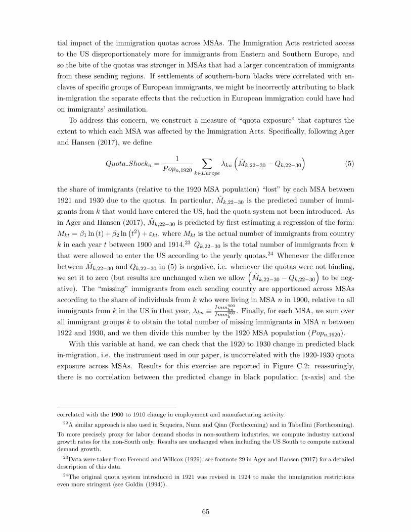
tial impact of the immigration quotas across MSAs. The Immigration Acts restricted access

to the US disproportionately more for immigrants from Eastern and Southern Europe, and

so the bite of the quotas was stronger in MSAs that had a larger concentration of immigrants

from these sending regions. If settlements of southern-born blacks were correlated with en-

claves of specific groups of European immigrants, we might be incorrectly attributing to black

in-migration the separate effects that the reduction in European immigration could have had

on immigrants’ assimilation.

To address this concern, we construct a measure of “quota exposure” that captures the

extent to which each MSA was affected by the Immigration Acts. Specifically, following Ager

and Hansen (2017), we define

Quota Shockn =1

Popn,1920

∑k∈Europe

λkn

(Mk,22−30 −Qk,22−30

)(5)

the share of immigrants (relative to the 1920 MSA population) “lost” by each MSA between

1921 and 1930 due to the quotas. In particular, Mk,22−30 is the predicted number of immi-

grants from k that would have entered the US, had the quota system not been introduced. As

in Ager and Hansen (2017), Mk,22−30 is predicted by first estimating a regression of the form:

Mkt = β1 ln (t) + β2 ln(t2)

+ εkt, where Mkt is the actual number of immigrants from country

k in each year t between 1900 and 1914.23 Qk,22−30 is the total number of immigrants from k

that were allowed to enter the US according to the yearly quotas.24 Whenever the difference

between Mk,22−30 and Qk,22−30 in (5) is negative, i.e. whenever the quotas were not binding,

we set it to zero (but results are unchanged when we allow(Mk,22−30 −Qk,22−30

)to be neg-

ative). The “missing” immigrants from each sending country are apportioned across MSAs

according to the share of individuals from k who were living in MSA n in 1900, relative to all

immigrants from k in the US in that year, λkn ≡Imm900

kn

Imm900k

. Finally, for each MSA, we sum over

all immigrant groups k to obtain the total number of missing immigrants in MSA n between

1922 and 1930, and we then divide this number by the 1920 MSA population (Popn,1920).

With this variable at hand, we can check that the 1920 to 1930 change in predicted black

in-migration, i.e. the instrument used in our paper, is uncorrelated with the 1920-1930 quota

exposure across MSAs. Results for this exercise are reported in Figure C.2: reassuringly,

there is no correlation between the predicted change in black population (x-axis) and the

correlated with the 1900 to 1910 change in employment and manufacturing activity.

22A similar approach is also used in Sequeira, Nunn and Qian (Forthcoming) and in Tabellini (Forthcoming).

To more precisely proxy for labor demand shocks in non-southern industries, we compute industry nationalgrowth rates for the non-South only. Results are unchanged when including the US South to compute nationaldemand growth.

23Data were taken from Ferenczi and Willcox (1929); see footnote 29 in Ager and Hansen (2017) for a detaileddescription of this data.

24The original quota system introduced in 1921 was revised in 1924 to make the immigration restrictionseven more stringent (see Goldin (1994)).

65

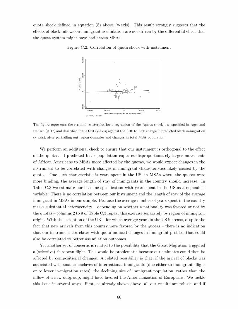
quota shock defined in equation (5) above (y-axis). This result strongly suggests that the

effects of black inflows on immigrant assimilation are not driven by the differential effect that

the quota system might have had across MSAs.

Figure C.2. Correlation of quota shock with instrument

−5

00

00

05

00

00

10

00

00

Qu

ota

sh

ock

−40000 −20000 0 20000 40000

1920−1930 change in predicted black population

coef=0.0714, p−value=0.807

The figure represents the residual scatterplot for a regression of the “quota shock”, as specified in Ager and

Hansen (2017) and described in the text (y-axis) against the 1910 to 1930 change in predicted black in-migration

(x-axis), after partialling out region dummies and changes in total MSA population.

We perform an additional check to ensure that our instrument is orthogonal to the effect

of the quotas. If predicted black population captures disproportionately larger movements

of African Americans to MSAs more affected by the quotas, we would expect changes in the

instrument to be correlated with changes in immigrant characteristics likely caused by the

quotas. One such characteristic is years spent in the US: in MSAs where the quotas were

more binding, the average length of stay of immigrants in the country should increase. In

Table C.3 we estimate our baseline specification with years spent in the US as a dependent

variable. There is no correlation between our instrument and the length of stay of the average

immigrant in MSAs in our sample. Because the average number of years spent in the country

masks substantial heterogeneity – depending on whether a nationality was favored or not by

the quotas – columns 2 to 9 of Table C.3 repeat this exercise separately by region of immigrant

origin. With the exception of the UK – for which average years in the US increase, despite the

fact that new arrivals from this country were favored by the quotas – there is no indication

that our instrument correlates with quota-induced changes in immigrant profiles, that could

also be correlated to better assimilation outcomes.

Yet another set of concerns is related to the possibility that the Great Migration triggered

a (selective) European flight. This would be problematic because our estimates could then be

affected by compositional changes. A related possibility is that, if the arrival of blacks was

associated with smaller enclaves of international immigrants (due either to immigrants flight

or to lower in-migration rates), the declining size of immigrant population, rather than the

inflow of a new outgroup, might have favored the Americanization of Europeans. We tackle

this issue in several ways. First, as already shown above, all our results are robust, and if

66

Tab

leC

.3.

Eff

ect

onav

erag

eye

ars

inth

eU

S

(1)

(2)

(3)

(4)

(5)

(6)

(7)

(8)

(9)

Dep

.va

riab

leA

vera

ge

years

inth

eU

S

All

nat

ion

alit

ies

Nor

ther

nE

UU

KIr

elan

dW

este

rnE

US

ou

ther

nE

UC

entr

al

an

dE

ast

ern

EU

Ger

many

Russ

ia

Nu

m.

bla

cks

0.09

7-0

.411

1.6

72∗

0.3

30

0.7

83

-0.2

51

-0.0

48

-0.6

48

-0.0

62

(0.4

06)

(0.4

47)

(0.9

03)

(0.6

71)

(0.5

52)

(0.1

79)

(0.5

22)

(0.6

83)

(0.3

32)

Ob

serv

atio

ns

15,8

89,4

091,

119,

820

1,359,7

59

1,2

17,5

39

463,4

89

2,7

77,1

17

3,3

21,0

56

1,9

64,4

97

2,1

62,9

93

R-s

qu

ared

0.60

60.

662

0.5

59

0.6

86

0.5

86

0.4

88

0.5

39

0.6

18

0.5

01

F-s

tat

24.6

427

.35

22.9

826.5

718.2

828.5

825.0

423.0

226.7

8

Note

s:T

he

analy

sis

isre

stri

cted

to108

non-s

outh

ern

MSA

sfo

rw

hic

hth

eIV

could

be

const

ruct

ed,

and

toyea

rs1910

to1930.

Colu

mn

1re

plica

tes

the

spec

ifica

tion

of

colu

mn

5,

Table

3,

wit

hout

indic

ato

rsfo

ryea

rsin

the

US.

Colu

mns

2-9

replica

teth

esp

ecifi

cati

on

inco

lum

n3

of

Table

3se

para

tely

for

each

regio

nof

ori

gin

.Sta

ndard

erro

rscl

ust

ered

at

the

MSA

level

inpare

nth

eses

.Sig

nifi

cance

level

s:∗∗∗

p<

0.0

1,

**

p<

0.0

5,

*p<

0.1

.

67

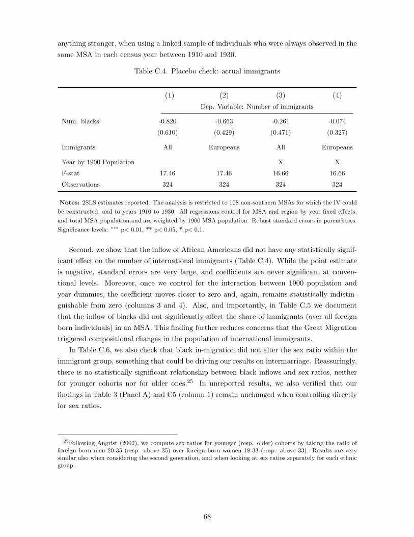
anything stronger, when using a linked sample of individuals who were always observed in the

same MSA in each census year between 1910 and 1930.

Table C.4. Placebo check: actual immigrants

(1) (2) (3) (4)

Dep. Variable: Number of immigrants

Num. blacks -0.820 -0.663 -0.261 -0.074

(0.610) (0.429) (0.471) (0.327)

Immigrants All Europeans All Europeans

Year by 1900 Population X X

F-stat 17.46 17.46 16.66 16.66

Observations 324 324 324 324

Notes: 2SLS estimates reported. The analysis is restricted to 108 non-southern MSAs for which the IV could

be constructed, and to years 1910 to 1930. All regressions control for MSA and region by year fixed effects,

and total MSA population and are weighted by 1900 MSA population. Robust standard errors in parentheses.

Significance levels: ∗∗∗ p< 0.01, ** p< 0.05, * p< 0.1.

Second, we show that the inflow of African Americans did not have any statistically signif-

icant effect on the number of international immigrants (Table C.4). While the point estimate

is negative, standard errors are very large, and coefficients are never significant at conven-

tional levels. Moreover, once we control for the interaction between 1900 population and

year dummies, the coefficient moves closer to zero and, again, remains statistically indistin-

guishable from zero (columns 3 and 4). Also, and importantly, in Table C.5 we document

that the inflow of blacks did not significantly affect the share of immigrants (over all foreign

born individuals) in an MSA. This finding further reduces concerns that the Great Migration

triggered compositional changes in the population of international immigrants.

In Table C.6, we also check that black in-migration did not alter the sex ratio within the

immigrant group, something that could be driving our results on intermarriage. Reassuringly,

there is no statistically significant relationship between black inflows and sex ratios, neither

for younger cohorts nor for older ones.25 In unreported results, we also verified that our

findings in Table 3 (Panel A) and C5 (column 1) remain unchanged when controlling directly

for sex ratios.

25Following Angrist (2002), we compute sex ratios for younger (resp. older) cohorts by taking the ratio offoreign born men 20-35 (resp. above 35) over foreign born women 18-33 (resp. above 33). Results are verysimilar also when considering the second generation, and when looking at sex ratios separately for each ethnicgroup.

68

Tab

leC

.5.

Ch

ange

inth

eet

hn

icco

mp

osit

ion

ofth

efo

reig

n-b

orn

(1)

(2)

(3)

(4)

(5)

(6)

(7)

(8)

Dep

.va

riab

leS

hare

of

imm

igra

nts

from

each

regio

n

Nor

ther

nE

UU

KIr

elan

dW

este

rnE

US

ou

ther

nE

UC

entr

al

an

dE

ast

ern

EU

Ger

many

Ru

ssia

Nu

m.

bla

cks

-0.0

07-0

.014

-0.0

14∗

-0.0

05

0.0

19

0.0

16

0.0

01

0.0

06

(0.0

05)

(0.0

09)

(0.0

07)

(0.0

04)

(0.0

12)

(0.0

17)

(0.0

22)

(0.0

13)

Ob

serv

atio

ns

324

324

324

324

324

324

324

324

R-s

qu

ared

0.15

70.

331

0.8

62

0.4

28

0.7

99

0.7

50

0.8

08

0.5

27

F-s

tat

17.4

617

.46

17.4

617.4

617.4

617.4

617.4

617.4

6

Note

s:T

he

analy

sis

isre

stri

cted

to108

non-s

outh

ern

MSA

sfo

rw

hic

hth

eIV

could

be

const

ruct

ed,

and

toyea

rs1910

to1930.

All

regre

ssio

ns

contr

ol

for

MSA

and

yea

rby

regio

nfixed

effec

t,to

tal

popula

tion

and

are

wei

ghte

dby

popula

tion

in1900.

Sta

ndard

erro

rscl

ust

ered

at

the

MSA

level

inpare

nth

eses

.Sig

nifi

cance

level

s:∗∗∗

p<

0.0

1,

**

p<

0.0

5,

*p<

0.1

.

69

Table C.6. Sex ratios

(1) (2) (3)

Dep. variable Sex ratios

All Young Old

Num. blacks -0.084 -0.042 -0.102

(0.102) (0.113) (0.089)

F-stat 17.46 17.46 17.46

Observations 324 324 324

Notes: The analysis is restricted to 108 non-southern MSAs for which the IV could be constructed, and to

years 1910 to 1930. All regressions control for MSA and year by region fixed effect, total population and are

weighted by population in 1900. Standard errors clustered at the MSA level in parentheses. Significance levels:∗∗∗ p< 0.01, ** p< 0.05, * p< 0.1.

Additionally, and to more directly tackle the potential concerns on the validity of Bar-

tik instruments discussed in Goldsmith-Pinkham, Sorkin and Swift (2018), we replicate our

analysis by interacting year dummies with the share of southern-born blacks from each state,

i.e. α1900jn in equation (2).26 We plot 2SLS coefficients from this exercise in Figure C.4 for

both intermarriage (Panel A) and naturalization rates (Panel B). The first point estimate on

the left plots the coefficient from our baseline specification (i.e. column 3 of Table 3), while

subsequent point estimates result from regressions including each interaction separately. As

it appears, with two exceptions, results for both intermarriage and naturalization rates are

very stable and remain close to the baseline effect. Only when interacting year dummies

with the share of African Americans from Georgia (resp. Delaware) the point estimate for

intermarriage (resp. naturalization) becomes smaller in magnitude and imprecisely estimated.

Overall, this exercise is reassuring for the validity of the instrument, since it suggests that

results are unlikely to be driven by any specific black enclave that happened to locate in e.g.

booming MSAs before 1900.

26Specifically, Goldsmith-Pinkham, Sorkin and Swift (2018) argue that the key identification assumptionbehind Bartik instruments is the exogeneity of the initial shares (α1900

jn ). Because of perfect multicollinearity,we cannot include interactions between year dummies and all the shares simultaneously. Hence, we performthis exercise by interacting year dummies with α1900

jn for each southern state j, one at the time.

70

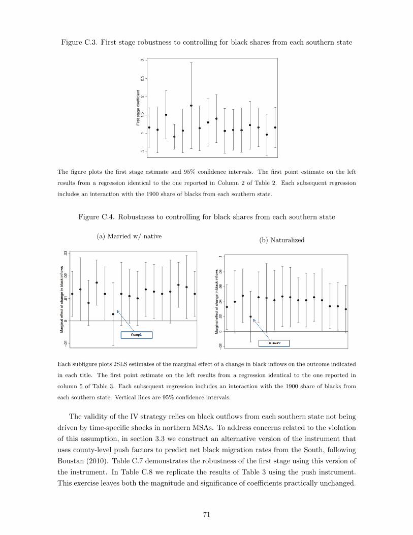
Figure C.3. First stage robustness to controlling for black shares from each southern state

.51

1.5

22

.53

First

sta

ge

co

eff

icie

nt

The figure plots the first stage estimate and 95% confidence intervals. The first point estimate on the left

results from a regression identical to the one reported in Column 2 of Table 2. Each subsequent regression

includes an interaction with the 1900 share of blacks from each southern state.

Figure C.4. Robustness to controlling for black shares from each southern state

(a) Married w/ native(b) Naturalized

Each subfigure plots 2SLS estimates of the marginal effect of a change in black inflows on the outcome indicated

in each title. The first point estimate on the left results from a regression identical to the one reported in

column 5 of Table 3. Each subsequent regression includes an interaction with the 1900 share of blacks from

each southern state. Vertical lines are 95% confidence intervals.

The validity of the IV strategy relies on black outflows from each southern state not being

driven by time-specific shocks in northern MSAs. To address concerns related to the violation

of this assumption, in section 3.3 we construct an alternative version of the instrument that

uses county-level push factors to predict net black migration rates from the South, following

Boustan (2010). Table C.7 demonstrates the robustness of the first stage using this version of

the instrument. In Table C.8 we replicate the results of Table 3 using the push instrument.

This exercise leaves both the magnitude and significance of coefficients practically unchanged.

71

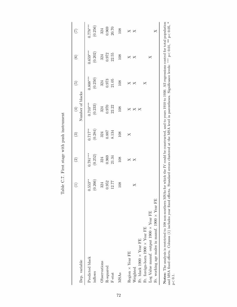
Tab

leC

.7.

Fir

stst

age

wit

hp

ush

inst

rum

ent

(1)

(2)

(3)

(4)

(5)

(6)

(7)

Dep

.va

riab

leN

um

ber

of

bla

cks

Pre

dic

ted

bla

ck0.5

53∗

∗0.7

81∗∗

∗0.7

17∗∗

0.7

10∗∗

∗0.8

08∗

∗∗0.6

59∗∗

∗0.7

78∗∗

∗

infl

ows

(0.2

66)

(0.2

52)

(0.2

84)

(0.2

33)

(0.2

50)

(0.2

02)

(0.2

56)

Ob

serv

atio

ns

324

324

324

324

324

324

324

R-s

qu

ared

0.9

52

0.9

69

0.8

87

0.9

70

0.9

73

0.9

72

0.9

69

F-s

tat

12.7

721.3

48.1

34

22.2

221.0

522.5

520.7

0

MS

As

108

108

108

108

108

108

108

Reg

ion×

Yea

rF

EX

XX

XX

X

Wei

ghte

dX

XX

XX

X

Fr.

bla

ck19

00×

Yea

rF

EX

Fr.

fore

ign

-bor

n19

00×

Yea

rF

EX

Log

Val

ue

man

uf.

outp

ut

1900×

Yea

rF

EX

Fr.

wor

kin

gag

em

ales

inm

anu

f.19

00×

Yea

rF

EX

Note

s:T

he

analy

sis

isre

stri

cted

to108

non-s

outh

ern

MSA

sfo

rw

hic

hth

eIV

could

be

const

ruct

ed,

and

toyea

rs1910

to1930.

All

regre

ssio

ns

contr

olfo

rto

talp

opula

tion

and

MSA

fixed

effec

ts.

Colu

mn

(1)

incl

udes

yea

rfixed

effec

ts.

Sta

ndard

erro

rscl

ust

ered

at

the

MSA

level

inpare

nth

eses

.Sig

nifi

cance

level

s:∗∗∗

p<

0.0

1,

**

p<

0.0

5,

*p<

0.1

.

72

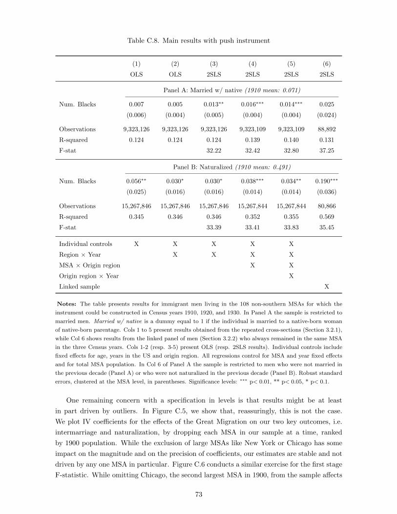
Table C.8. Main results with push instrument

(1) (2) (3) (4) (5) (6)

OLS OLS 2SLS 2SLS 2SLS 2SLS

Panel A: Married w/ native (1910 mean: 0.071)

Num. Blacks 0.007 0.005 0.013∗∗ 0.016∗∗∗ 0.014∗∗∗ 0.025

(0.006) (0.004) (0.005) (0.004) (0.004) (0.024)

Observations 9,323,126 9,323,126 9,323,126 9,323,109 9,323,109 88,892

R-squared 0.124 0.124 0.124 0.139 0.140 0.131

F-stat 32.22 32.42 32.80 37.25

Panel B: Naturalized (1910 mean: 0.491)

Num. Blacks 0.056∗∗ 0.030∗ 0.030∗ 0.038∗∗∗ 0.034∗∗ 0.190∗∗∗

(0.025) (0.016) (0.016) (0.014) (0.014) (0.036)

Observations 15,267,846 15,267,846 15,267,846 15,267,844 15,267,844 80,866

R-squared 0.345 0.346 0.346 0.352 0.355 0.569

F-stat 33.39 33.41 33.83 35.45

Individual controls X X X X X

Region × Year X X X X

MSA × Origin region X X

Origin region × Year X

Linked sample X

Notes: The table presents results for immigrant men living in the 108 non-southern MSAs for which the

instrument could be constructed in Census years 1910, 1920, and 1930. In Panel A the sample is restricted to

married men. Married w/ native is a dummy equal to 1 if the individual is married to a native-born woman

of native-born parentage. Cols 1 to 5 present results obtained from the repeated cross-sections (Section 3.2.1),

while Col 6 shows results from the linked panel of men (Section 3.2.2) who always remained in the same MSA

in the three Census years. Cols 1-2 (resp. 3-5) present OLS (resp. 2SLS results). Individual controls include

fixed effects for age, years in the US and origin region. All regressions control for MSA and year fixed effects

and for total MSA population. In Col 6 of Panel A the sample is restricted to men who were not married in

the previous decade (Panel A) or who were not naturalized in the previous decade (Panel B). Robust standard

errors, clustered at the MSA level, in parentheses. Significance levels: ∗∗∗ p< 0.01, ** p< 0.05, * p< 0.1.

One remaining concern with a specification in levels is that results might be at least

in part driven by outliers. In Figure C.5, we show that, reassuringly, this is not the case.

We plot IV coefficients for the effects of the Great Migration on our two key outcomes, i.e.

intermarriage and naturalization, by dropping each MSA in our sample at a time, ranked

by 1900 population. While the exclusion of large MSAs like New York or Chicago has some

impact on the magnitude and on the precision of coefficients, our estimates are stable and not

driven by any one MSA in particular. Figure C.6 conducts a similar exercise for the first stage

F-statistic. While omitting Chicago, the second largest MSA in 1900, from the sample affects

73

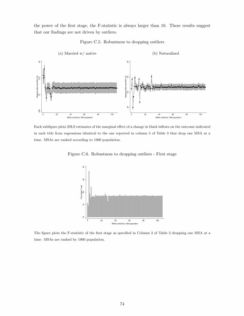
the power of the first stage, the F-statistic is always larger than 10. These results suggest

that our findings are not driven by outliers.

Figure C.5. Robustness to dropping outliers

(a) Married w/ native

.005

.01

.015

.02

Marg

inal effect and 9

5%

CIs

0 20 40 60 80 100

MSAs ranked by 1900 population

(b) Naturalized

.02

.03

.04

.05

Marg

inal effect and 9

5%

CIs

0 20 40 60 80 100

MSAs ranked by 1900 population

Each subfigure plots 2SLS estimates of the marginal effect of a change in black inflows on the outcome indicated

in each title from regressions identical to the one reported in column 5 of Table 3 that drop one MSA at a

time. MSAs are ranked according to 1900 population.

Figure C.6. Robustness to dropping outliers - First stage

10

15

20

25

30

First

sta

ge

F−

sta

t

0 20 40 60 80 100

MSAs ranked by 1900 population

The figure plots the F-statistic of the first stage as specified in Column 2 of Table 2 dropping one MSA at a

time. MSAs are ranked by 1900 population.

74

D Additional outcomes

D.1 Additional Economic and Social Outcomes

In Section 4, we showed that the Great Migration increased the probability of intermarriage

between immigrants and native-born whites. We interpreted these findings as evidence that

black inflows fostered assimilation of the previous outgroup. We also showed that the arrival of

African Americans fostered immigrants’ effort to assimilate, proxied as the share of naturalized

immigrants. Here, we present results using manufacturing employment as a proxy of economic

assimilation, and name choices for immigrant children as an alternative measure of assimilation

effort.

In Panel A of Table D.1, the dependent variable is a dummy equal to one for work-

ing in manufacturing, which was the “immigrant-intensive” sector at the time. Both OLS

and 2SLS estimates are strongly negative and statistically significant in all our specifications

and samples. Unlike the case of intermarriage, OLS coefficients are less negative than the

corresponding 2SLS ones. That the direction of the OLS bias is not the same for social and

economic assimilation is not entirely surprising – blacks were most likely attracted by econom-

ically booming MSAs, in which immigrants were able to experience occupational upgrading.

At the same time, it was those same MSAs that attracted more new migrants and potentially

saw the formation of migrant enclaves (Eriksson and Ward, 2018), factors that could have

hindered the social integration of immigrants.

The effects of the Great Migration are economically relevant: the coefficient in column

3 of Table D.1 (Panel A) implies that one standard deviation increase in the number of

African Americans lowers the share of immigrants working in the manufacturing sector by 2.5

percentage points, or 10% relative to the 1910 mean. Since manufacturing was an immigrant-

instensive sector at the time, these results can be interpreted as occupational upgrading and

economic assimilation.

Panel B of Table D.1 presents results for first names given to the children of immigrants

born in the US. We use the logarithm of the foreign name index as dependent variable to

facilitate the interpretation of coefficients in percentage terms. We do not construct the index

in the panel dataset, which consists of foreign-born individuals whose names were decided in

their country of origin. Black inflows significantly lower the foreign name index of immigrant

children and the effect is robust to the inclusion of controls. The estimated magnitude implies

that the inflow of 100,000 blacks – or, less than half of those received by Chicago – led to a

change in Italian names equivalent to that from Luciano to Mike, and a change in Russian

names equivalent to that from Stanislav to Morris or Max.

In Table D.2, we explore the robustness of our main results to the use of alternative proxies

for successful assimilation, and investigate the effects of the Great Migration on additional

outcomes.

First, we proxy for occupational or skill upgrading using the share of immigrants working

in the unskilled sector. As it appears, consistent with our findings for manufacturing (see

Table D.1, Panel A), there is a negative and significant effect of black inflows on the share of

75

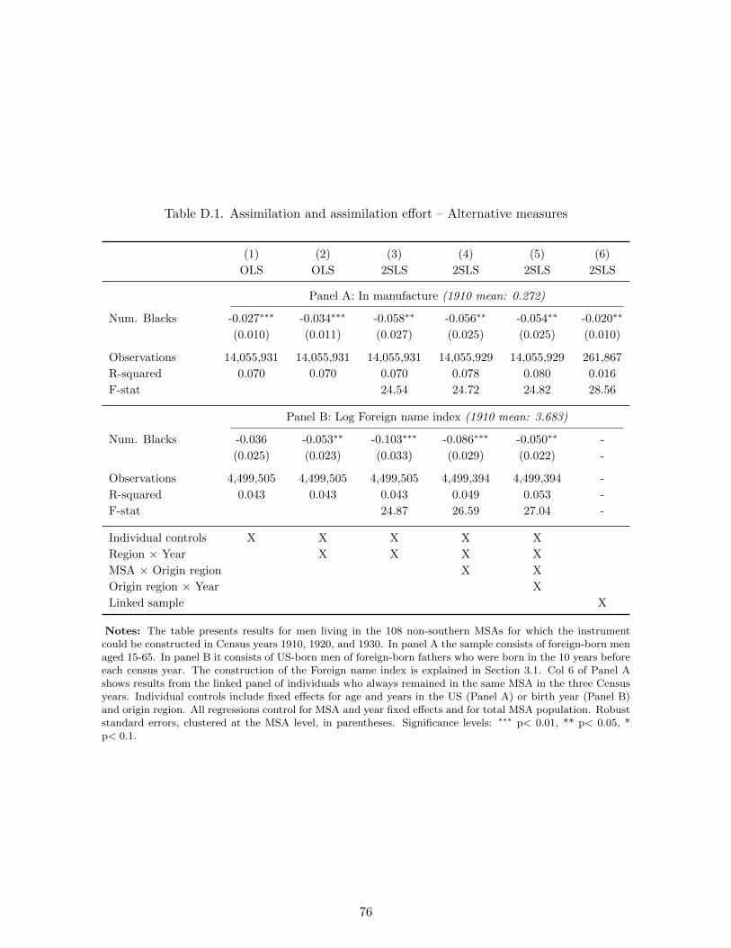
Table D.1. Assimilation and assimilation effort – Alternative measures

(1) (2) (3) (4) (5) (6)

OLS OLS 2SLS 2SLS 2SLS 2SLS

Panel A: In manufacture (1910 mean: 0.272)

Num. Blacks -0.027∗∗∗ -0.034∗∗∗ -0.058∗∗ -0.056∗∗ -0.054∗∗ -0.020∗∗

(0.010) (0.011) (0.027) (0.025) (0.025) (0.010)

Observations 14,055,931 14,055,931 14,055,931 14,055,929 14,055,929 261,867

R-squared 0.070 0.070 0.070 0.078 0.080 0.016

F-stat 24.54 24.72 24.82 28.56

Panel B: Log Foreign name index (1910 mean: 3.683)

Num. Blacks -0.036 -0.053∗∗ -0.103∗∗∗ -0.086∗∗∗ -0.050∗∗ -

(0.025) (0.023) (0.033) (0.029) (0.022) -

Observations 4,499,505 4,499,505 4,499,505 4,499,394 4,499,394 -

R-squared 0.043 0.043 0.043 0.049 0.053 -

F-stat 24.87 26.59 27.04 -

Individual controls X X X X X

Region × Year X X X X

MSA × Origin region X X

Origin region × Year X

Linked sample X

Notes: The table presents results for men living in the 108 non-southern MSAs for which the instrumentcould be constructed in Census years 1910, 1920, and 1930. In panel A the sample consists of foreign-born menaged 15-65. In panel B it consists of US-born men of foreign-born fathers who were born in the 10 years beforeeach census year. The construction of the Foreign name index is explained in Section 3.1. Col 6 of Panel Ashows results from the linked panel of individuals who always remained in the same MSA in the three Censusyears. Individual controls include fixed effects for age and years in the US (Panel A) or birth year (Panel B)and origin region. All regressions control for MSA and year fixed effects and for total MSA population. Robuststandard errors, clustered at the MSA level, in parentheses. Significance levels: ∗∗∗ p< 0.01, ** p< 0.05, *p< 0.1.

76

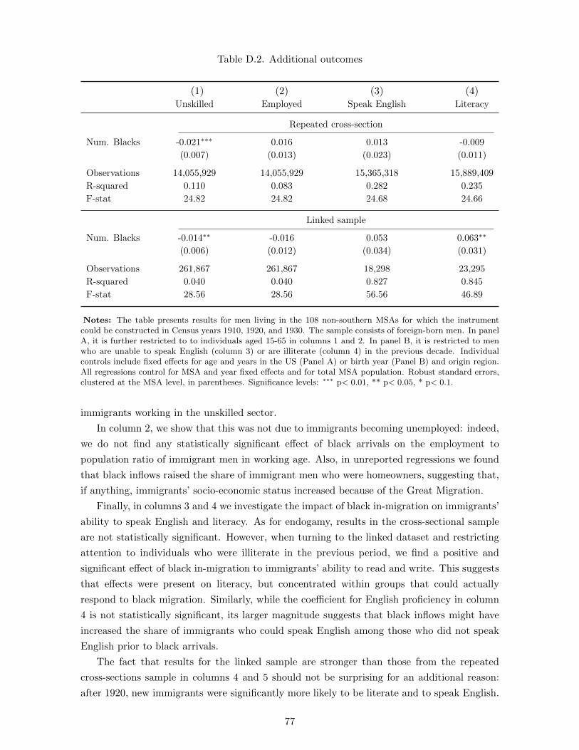
Table D.2. Additional outcomes

(1) (2) (3) (4)Unskilled Employed Speak English Literacy

Repeated cross-section

Num. Blacks -0.021∗∗∗ 0.016 0.013 -0.009

(0.007) (0.013) (0.023) (0.011)

Observations 14,055,929 14,055,929 15,365,318 15,889,409

R-squared 0.110 0.083 0.282 0.235

F-stat 24.82 24.82 24.68 24.66

Linked sample

Num. Blacks -0.014∗∗ -0.016 0.053 0.063∗∗

(0.006) (0.012) (0.034) (0.031)

Observations 261,867 261,867 18,298 23,295

R-squared 0.040 0.040 0.827 0.845

F-stat 28.56 28.56 56.56 46.89

Notes: The table presents results for men living in the 108 non-southern MSAs for which the instrumentcould be constructed in Census years 1910, 1920, and 1930. The sample consists of foreign-born men. In panelA, it is further restricted to to individuals aged 15-65 in columns 1 and 2. In panel B, it is restricted to menwho are unable to speak English (column 3) or are illiterate (column 4) in the previous decade. Individualcontrols include fixed effects for age and years in the US (Panel A) or birth year (Panel B) and origin region.All regressions control for MSA and year fixed effects and for total MSA population. Robust standard errors,clustered at the MSA level, in parentheses. Significance levels: ∗∗∗ p< 0.01, ** p< 0.05, * p< 0.1.

immigrants working in the unskilled sector.

In column 2, we show that this was not due to immigrants becoming unemployed: indeed,

we do not find any statistically significant effect of black arrivals on the employment to

population ratio of immigrant men in working age. Also, in unreported regressions we found

that black inflows raised the share of immigrant men who were homeowners, suggesting that,

if anything, immigrants’ socio-economic status increased because of the Great Migration.

Finally, in columns 3 and 4 we investigate the impact of black in-migration on immigrants’

ability to speak English and literacy. As for endogamy, results in the cross-sectional sample

are not statistically significant. However, when turning to the linked dataset and restricting

attention to individuals who were illiterate in the previous period, we find a positive and

significant effect of black in-migration to immigrants’ ability to read and write. This suggests

that effects were present on literacy, but concentrated within groups that could actually

respond to black migration. Similarly, while the coefficient for English proficiency in column

4 is not statistically significant, its larger magnitude suggests that black inflows might have

increased the share of immigrants who could speak English among those who did not speak

English prior to black arrivals.

The fact that results for the linked sample are stronger than those from the repeated

cross-sections sample in columns 4 and 5 should not be surprising for an additional reason:

after 1920, new immigrants were significantly more likely to be literate and to speak English.

77

On the one hand, the literacy test of 1917 restricted access to the US to immigrants who

could read and write. On the other, the Immigration Acts of the 1920s disproportionately

favored immigrant groups that were more skilled and whose linguistic distance from English

was lower (i.e. those from Western and Northern Europe). It follows that the “margin of

adjustment” for these outcomes was certainly larger for immigrants arrived in the US before

1915, i.e. those that we observe in the linked sample, than for more recent ones.

D.2 Residential Segregation

Given the close-link between social identity and geographic segregation (Echenique and Fryer,

Jr., 2007; Card, Mas and Rothstein, 2008; Gentzkow and Shapiro, 2011; Enos, 2017; Logan and

Parman, 2017), we investigate whether there is a link between the arrival of African Americans

as a result of the Great Migration and patterns of residential segregation. Building on a new

method developed by Logan and Parman (2017) we use information on the relative locations

of household heads to calculate ethnic segregation. This method utilizes the way in which

census enumerators traversed around geographies to induct the identity of a given household’s

neighbors. In particular, it is based on the relative ordering on a census enumeration form as

a proxy for the geographic location of one’s neighbors. For example, if the household head

enumerated right before a given household head is an immigrant, then this measure codes that

given household head as being neighbors with an immigrant. From this, one can calculate a

neighbor-based index of segregation along any binary dimension. Using the complete count

U.S. Censuses from 1910-1930 we construct a measure of segregation on the basis of the

country of birth of (first-generation) European immigrants. Specifically, we compute

Segregation =E(xc)− xc

E(xc)− E(xc)

where xc is the number of households nationality n (as defined by the household head) with

a next-door neighbor of a different nationality. E(xc) is the expected number of households

with neighbors of different nationality under random assignment of neighbors, and E(xc) is

the respective number under complete segregation.27 We calculate four different versions that

adjust for the presence of foreign-born non co-nationals on either side of a given household and

for the presence of foreign-born non co-nationals on both sides, in addition to adjusting the

measure to look at neighbors on the same street among the households for which we have data

on street names. We denote these outcomes as Segregation(P −One) and Segregation(P −Both) when not adjusting for streets and using information on one or both sides respectively,

in addition to Segregation(S−One) and Segregation(S−Both) when adjusting for streets.28

We compute these measures at the MSA-level for the sixteen European countries that had

27For more details on the construction of the measure and its comparison with traditional indices of segre-gation we refer readers to Logan and Parman (2017).

28The correlation among all of these measures is generally quite high.

78

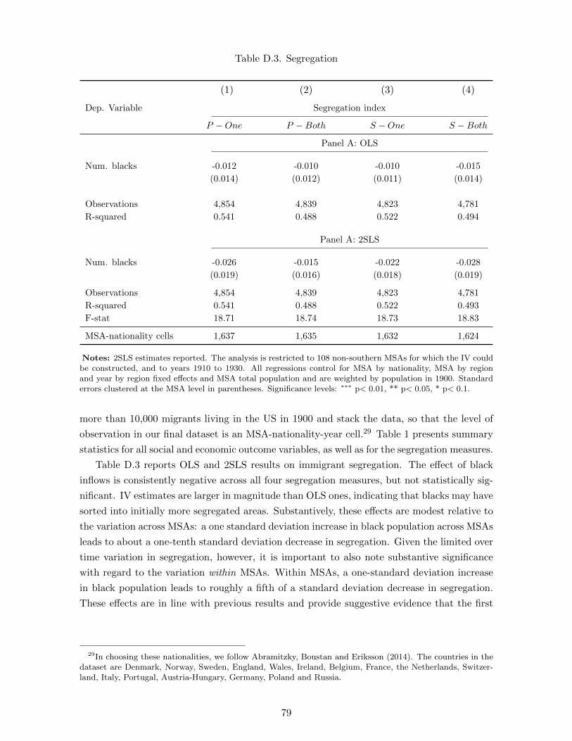
Table D.3. Segregation

(1) (2) (3) (4)

Dep. Variable Segregation index

P −One P −Both S −One S −Both

Panel A: OLS

Num. blacks -0.012 -0.010 -0.010 -0.015

(0.014) (0.012) (0.011) (0.014)

Observations 4,854 4,839 4,823 4,781

R-squared 0.541 0.488 0.522 0.494

Panel A: 2SLS

Num. blacks -0.026 -0.015 -0.022 -0.028

(0.019) (0.016) (0.018) (0.019)

Observations 4,854 4,839 4,823 4,781

R-squared 0.541 0.488 0.522 0.493

F-stat 18.71 18.74 18.73 18.83

MSA-nationality cells 1,637 1,635 1,632 1,624

Notes: 2SLS estimates reported. The analysis is restricted to 108 non-southern MSAs for which the IV couldbe constructed, and to years 1910 to 1930. All regressions control for MSA by nationality, MSA by regionand year by region fixed effects and MSA total population and are weighted by population in 1900. Standarderrors clustered at the MSA level in parentheses. Significance levels: ∗∗∗ p< 0.01, ** p< 0.05, * p< 0.1.

more than 10,000 migrants living in the US in 1900 and stack the data, so that the level of

observation in our final dataset is an MSA-nationality-year cell.29 Table 1 presents summary

statistics for all social and economic outcome variables, as well as for the segregation measures.

Table D.3 reports OLS and 2SLS results on immigrant segregation. The effect of black

inflows is consistently negative across all four segregation measures, but not statistically sig-

nificant. IV estimates are larger in magnitude than OLS ones, indicating that blacks may have

sorted into initially more segregated areas. Substantively, these effects are modest relative to

the variation across MSAs: a one standard deviation increase in black population across MSAs

leads to about a one-tenth standard deviation decrease in segregation. Given the limited over

time variation in segregation, however, it is important to also note substantive significance

with regard to the variation within MSAs. Within MSAs, a one-standard deviation increase

in black population leads to roughly a fifth of a standard deviation decrease in segregation.

These effects are in line with previous results and provide suggestive evidence that the first

29In choosing these nationalities, we follow Abramitzky, Boustan and Eriksson (2014). The countries in thedataset are Denmark, Norway, Sweden, England, Wales, Ireland, Belgium, France, the Netherlands, Switzer-land, Italy, Portugal, Austria-Hungary, Germany, Poland and Russia.

79

Great Migration led to immigrants’ residential assimilation with native-born whites.

80

E A simple theoretical framework

E.1 Basic model

We build a simple theory, relying on core findings of the social psychology literature on

categorization (Turner et al., 1987), in order to formalize the effects that black inflows have

on native-born whites’ attitudes and immigrant outcomes. Our goal is not to explain the

cognitive processes that reduced native-born prejudice towards immigrants after the Great

Migration. Instead, we assume that a cognitive mechanism led native-born whites to re-

categorize immigrants as members of the ingroup, and explore the theoretical and empirical

implications of that assumption.

Setup

The population consists of two groups, an ingroup and an outgroup. For our purposes we

define the ingroup to be the group containing native-born whites of Anglo-Saxon origin, and

the outgroup to be everyone else. Prior to the Great Migration, the outgroup consists of

immigrants of European descent, but later on is expanded to include African Americans.

Building on a large literature in social psychology documenting the existence of consensual

ethnic and racial hierarchies in social distance in multiethnic and multiracial societies (Berry

and Kalin, 1979; Duckitt, 1994; Hagendoorn, 1995), we define h to be the social distance of

outgroup members from the group of native-born whites. h can be thought of as a unidimen-

sional summary measure of distances along multiple dimensions, such as skin color, language,

culture or religion. Native whites are share n of the population and have h = 0. outgroup

members are a share 1− n of the population and are distributed on the line [0, Hmax].

We assume that native-born whites engage in taste-based discrimination. In particular,

we assume that interactions with individuals who are distant to them (h > 0) induce a

psychological cost for native-born whites. This cost depends on perceived distance λ(h, h),

where h is the average distance of the outgroup from the ingroup. h can be thought of as

the degree of difference between a native-born white and the members of the outgroup he is

faced with on average in his daily life or in his neighborhood. As such, it captures the degree

of white native-born whites’ familiarity with more distant “outsiders”. Perceived distance is

increasing in actual distance and so λh > 0 and λh < 0. Furthermore, λ(0, h) = 0 for any h.

Crucially, we assume that λh,h ≤ 0, since higher average familiarity with more distant

outgroup members makes an outsider of any given distance appear more similar to native-

born whites. This assumption is one of the core tenets of self categorization theory, known as

the meta contrast principle (Turner et al., 1987, 1994). Categorization of stimuli into groups

is context-dependent. Humans are more likely to classify a collection of stimuli as a single

grouping if differences between those stimuli are smaller than differences between the grouping

that they form and other groupings. In our case, an immigrant is more likely to be classified

as a member of the ingroup if the difference in social distance between the immigrant and the

native-born whites is smaller than the difference between the average distance of the ingroup

81

and the outgroup (h).30

Other than through higher average outgroup distance, the disutility that native-born

whites endure when interacting with outsiders can be further reduced through the efforts that

outgroup members themselves exert in order to assimilate. This assimilation effort, denoted

by e, encompasses a range of behaviors that reduce the outgroup’s perceived distance to the

ingroup, such as learning their language, adopting their habits and mode of dress, or their

characteristic naming patterns.

Discrimination. With each interaction, native-born whites are faced with a binary decision

of whether to treat an individual as a member of their group or as an outsider, that is,

whether to engage in discriminatory behavior. Discrimination relieves native-born whites

of the psychological cost of interacting with distant others, but it comes at a cost F , which

captures both the actual effort of engaging in discriminatory behavior and the cost of foregone

monetary or social transactions with members of the outgroup. We denote the decision to

discriminate or not by d ∈ [0, 1], so that utility for an ingroup member is given by

U =

−W (λ, e), if d = 0

−F, if d = 1

where W is the psychological cost of interacting with an individual at perceived distance λ

and who provides effort e, with Wλ > 0, We < 0 and Wλ,e < 0. W (0, e) = 0 for any e. Native

whites engage in discrimination whenever its benefits exceed its costs, so whenever W > F .

Assimilation decisions of outgroup members. outgroup members provide assimilation

effort in the hope of becoming part of the native-born white ingroup. Membership in the

native-born white group confers benefits, both material (e.g. access to better jobs or housing)

and psychological (e.g. avoiding the cost of discrimination or harassment). The problem of

outgroup members is given by

maxeP (e, h)B − c(e)

where B is the benefit from assimilation and c is a convex cost function with c(0) = 0.

P (e, h) is an indicator for successful assimilation and thus P = 1(F > W ). Consequently,

Pe ≥ 0, Ph ≤ 0, and Peh ≥ 0.

The minimum amount of effort needed to ensure assimilation into the native-born white

group is implicitly defined by

F = W (λ,¯e(h)) (6)

30A related, though multidimensional, framework emphasizing context dependence with similar predictionson reclassification is the literature on stereotypes (Bordalo et al., 2016), which relies on the representativenessheuristic (Kahneman and Tversky, 1974).

82

outgroup members can decide between exerting effort¯e and enjoying the benefits of as-

similation at cost c(e), or avoiding the costs of effort and foregoing the assimilation bene-

fit. An outgroup member of type h will thus provide assimilation effort e =¯e(h) whenever

B > c(¯e(h)) and choose e = 0 otherwise. To ensure an interior solution we will always assume

c(e(Hmax)) > B.

Proposition 1. There exists a threshold h∗, given by B = (¯e(h∗)), such that individuals

with a distance below h∗ optimally choose to provide sufficient assimilation effort to ensure

integration in the native-born white group. Those with a distance exceeding h∗ provide zero

effort and do not become assimilated. Formally,

e∗ =

¯e(h), for h ≤ h∗

0, for h > h∗(7)

Proof. If h = 0 then¯e(h = 0) = 0 and c(0) = 0 which is less than B, so immigrants of

distance h = 0 will provide sufficient effort to reap the assimilation benefit.

If h = Hmax we assumed that c(e(Hmax)) > B, so immigrants of distance h = Hmax will

provide no effort and will not become assimilated.

From equation 6, the implicit function theorem gives that eh = −WhWe

> 0, so that the

minimum effort necessary for assimilation, as well as its associated costs, are increasing in an

outgroup member’s distance from the native-born white group.

The appearance of a more distant outgroup

In this context, we can think of the increasing presence of African Americans in the North

as an increase in Hmax, the perceived distance of the most distant outgroup member. While

no studies measure the precise social distance hierarchy in the early 20th century United

States, studies in later years and in a number of countries suggest a clear ranking, with

Northern Europeans at the top and Africans at the bottom. This ranking is furthermore

agreed upon by members of all ethnic and racial groups (Berry and Kalin, 1979; Duckitt,

1994; Pettigrew, 1960). Our assumption builds on this empirical literature. This gives us the

following proposition:

Proposition 2. An increase in Hmax leads to an increase in h∗.

Proof. An increase in Hmax raises h, or the average distance of the outgroup from the

white natives. Writing 6 explicitly as

F = W (λ(h, h),¯e(h, h))

we get immediately that

eh = −Wh

We< 0

83

so that for all outgroup members of a given distance h, necessary assimilation effort is

reduced. This implies that after the inflow of African Americans we have B > (¯e(h∗1)) with h∗1

denoting the old level of the distance threshold that guaranteed assimilation. Since eh > 0,

the new threshold level h∗2 for which B = (¯e(h∗2)) must be greater than h∗1. Thus, the arrival of

a new outgroup that is more distant to existing ones will necessarily increase the share of ex-

isting outgroup members that are allowed membership into the native-born white ingroup.31

The increase in distance of the most distant outgroup member has implications for the

optimal level of effort exerted by outgroup members of different types h. In particular, there

is an intermediate range of types who would not have optimally exerted assimilation effort

under the old distance cutoff, but who now find it profitable to do so.

The empirical implication of Proposition 2 is that immigrant assimilation should increase

on average in response to the Great Migration. This is our main empirical result presented in

Section 4. This prediction directly follows from the assumption that the psychological cost of

native-born whites is decreasing in the average distance of the outgroup. More interestingly,

the model generates testable implications on heterogeneous patterns of assimilation. Specifi-

cally, we can state the effects of an increase in Hmax on the optimal assimilation effort exerted

by outgroup members as a function of their type in the following proposition.

Proposition 3. Consider an increase in Hmax from Hmax1 to Hmax

2 and the corresponding

increase in the threshold distance level for assimilation from h∗1 to h∗2. Denote with e∗1(h) and

e∗2(h) the optimal level of effort provided by an immigrant of distance h, before and after the

increase in Hmax, respectively. We then havee∗2(h) ≤ e∗1(h), if h ≤ h∗1e∗2(h) > e∗1(h), if h∗1 < h ≤ h∗2e∗2(h) = e∗1(h) = 0, if h > h∗2

Proof. If h ≤ h∗1 an immigrant provides the minimum necessary effort both before and

after the increase. Since for any h¯e goes down when Hmax increases, immigrants who provide

¯e decrease their optimal level of provided effort. An immigrant with h > h∗1 has provided zero

effort under Hmax1 . If h ≤ h∗2 immigrants now provide the (strictly positive) necessary effort

level to ensure assimilation and if h > h∗2 then efforts stay at zero.

Proposition 3 implies that the inflow of African Americans has a different effect on each

of three distinct groups of immigrants, characterized by their baseline distance from the

31The accentuation component of self categorization theory implies that people classify objects into groups inorder to minimize within group differences and maximize across group differences (Turner et al., 1994; Haslamet al., 1995). This classification rule directly generates re-classification of white Europeans as members of theingroup when African Americans arrive and increase the variance of the outgroup. Fryer and Jackson (2008)show that this rule of classification can derive from a utility maximization problem. Gennaioli and Tabellini(2018) rely on a similar assumption to study political identities.

84

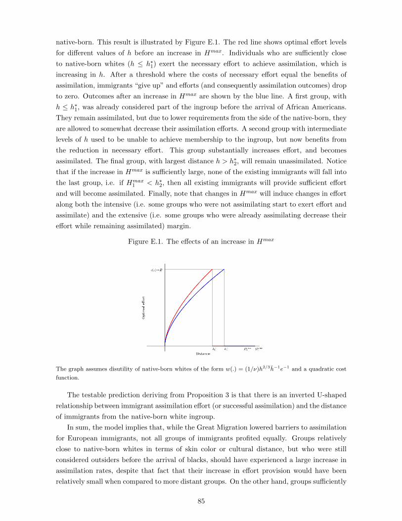
native-born. This result is illustrated by Figure E.1. The red line shows optimal effort levels

for different values of h before an increase in Hmax. Individuals who are sufficiently close

to native-born whites (h ≤ h∗1) exert the necessary effort to achieve assimilation, which is

increasing in h. After a threshold where the costs of necessary effort equal the benefits of

assimilation, immigrants “give up” and efforts (and consequently assimilation outcomes) drop

to zero. Outcomes after an increase in Hmax are shown by the blue line. A first group, with

h ≤ h∗1, was already considered part of the ingroup before the arrival of African Americans.

They remain assimilated, but due to lower requirements from the side of the native-born, they

are allowed to somewhat decrease their assimilation efforts. A second group with intermediate

levels of h used to be unable to achieve membership to the ingroup, but now benefits from

the reduction in necessary effort. This group substantially increases effort, and becomes

assimilated. The final group, with largest distance h > h∗2, will remain unassimilated. Notice

that if the increase in Hmax is sufficiently large, none of the existing immigrants will fall into

the last group, i.e. if Hmax1 < h∗2, then all existing immigrants will provide sufficient effort

and will become assimilated. Finally, note that changes in Hmax will induce changes in effort

along both the intensive (i.e. some groups who were not assimilating start to exert effort and

assimilate) and the extensive (i.e. some groups who were already assimilating decrease their

effort while remaining assimilated) margin.

Figure E.1. The effects of an increase in Hmax

The graph assumes disutility of native-born whites of the form w(.) = (1/ν)h2/3h−1e−1 and a quadratic cost

function.

The testable prediction deriving from Proposition 3 is that there is an inverted U-shaped

relationship between immigrant assimilation effort (or successful assimilation) and the distance

of immigrants from the native-born white ingroup.

In sum, the model implies that, while the Great Migration lowered barriers to assimilation

for European immigrants, not all groups of immigrants profited equally. Groups relatively

close to native-born whites in terms of skin color or cultural distance, but who were still

considered outsiders before the arrival of blacks, should have experienced a large increase in

assimilation rates, despite that fact that their increase in effort provision would have been

relatively small when compared to more distant groups. On the other hand, groups sufficiently

85

far away would not have benefited enough from reduced prejudice to become part of the

ingroup in significant numbers. In the following section we test and find support for these

predictions in the data.

E.2 Stochastic extension

So far, assimilation was assumed to be a deterministic process. We now generalize the model

and include stochastic individual level characteristics that alter an outgroup member’s as-

similation outlook. Let the disutility that an ingroup member suffers from interaction with

outgroup member be given by

W (λ, e) + µ

where µ ∼ N(0, σ2), representing unalterable characteristics of the individual. We assume

that its value is unknown to the individual at the time when effort provision is decided. This

may be due to the fact that outgroup members cannot properly predict how the ingroup will

respond to their personal characteristics in specific interactions.

The outgroup member then solves

maxePr(F > W (λ, e) + µ)B − c(e)

which can be written as

maxeG(F −W (λ, e))B − c(e)

where G() represents the cdf of µ. The first order condition for a relative extremum is then

g(F −W (λ, e))(−We)B = c′(e)

so that the marginal costs of effort are equalized to the pdf of µ, scaled by the benefits of

assimilation and the marginal effect of effort on the psychological costs of native-born whites.

To make progress with the generalized model, we specify that this disutility W is linear in λ

and e and that costs of effort are quadratic, in particular

W = ω1λ− ω2e

c = ce2

with ω1, ω2 and c > 0. Finally we will assume that λh,h = 0, implying that a change in h

86

has the same immediate effect on all outgroup members32. Optimal effort is then implicitly

defined by

g(F −W (λ, e∗))ω2B = 2ce∗

We then derive the effect of a marginal increase in h on e∗, given by

∂e∗

∂h=g′(.)B(−λh)ω1ω2

2c− g′(.)Bω22

(8)

which is positive as long as g′(.) is positive. Thus individuals respond to a larger h with an

increase in their assimilation efforts, as long as they had an initial assimilation probability of

less then 50%, and reduce efforts otherwise.

Equation (8) also shows that the response in effort has an inverted U-shape. The effect

of h on e∗ is increasing in g′() and thus maximal for individuals with h such that F −W (λ(h, h), e∗(h, )) = −σ. Effects are monotonically decreasing as h moves away from h in

either direction. A similar result holds for resulting rates of assimilation into the ingroup.

Assimilation rates of individuals with distance h are given by

A(h, h) = Pr(F > W (λ, e∗) + µ) = G(F −W (λ(h, h), e∗(h, h))

where individuals with a lower h always have higher equilibrium assimilation rates. The

response of assimilation rates to an increase in h is

dA(h, h)

dh= g(F −W (λ, e∗))

[(−ω1λh) + ω2

∂e∗

∂h

]> 0

Notice that, from the previous discussion, the expression in brackets on the right hand

side is unimodal with peak at h, while the density g() is naturally unimodal and maximized at

a value˜h,

˜h < h such that F = W (λ(

˜h, h), e∗(

˜h, h)). The resulting response in A is thus also

unimodal with a peak at hA, with h > hA >˜h. In other words, the response in assimilation

rates to an increase in h is also of inverted U-shape, but unlike assimilation efforts, the largest

responses will be among individuals with relatively low distance h.

We summarize this finding in the following proposition.

Proposition 4. The responses of optimal effort and of assimilation rates to an increase in

Hmax are both unimodal with respect to distance h. The peak of assimilation rates occurs at

a lower level of h than the peak of optimal effort.

We illustrate this result with a specific example, considering the functional form W =

ω1h − ω3h − ω2e and parameter values ω1 = 3, ω2 = ω3 = c = σ = 1, B = F = 0.5 and an

increase of Hmax from 1 to 1.5. Figure (E.2) plots optimal effort (left panel) and assimilation

32We also assume that σ is sufficiently large so that g′(−σ)ω22B < 2c and the marginal cost curves thus

crosses the scaled pdf only once

87

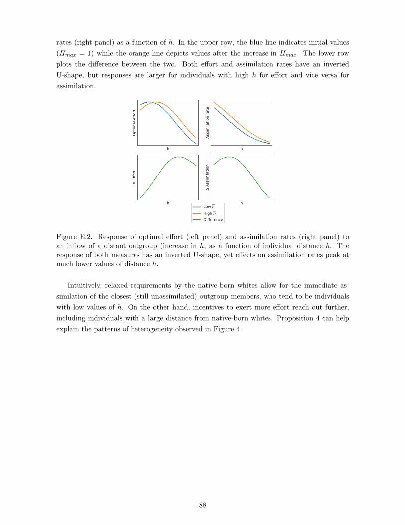
rates (right panel) as a function of h. In the upper row, the blue line indicates initial values

(Hmax = 1) while the orange line depicts values after the increase in Hmax. The lower row

plots the difference between the two. Both effort and assimilation rates have an inverted

U-shape, but responses are larger for individuals with high h for effort and vice versa for

assimilation.

h

Optim

al effo

rt

h

Assim

ilatio

n rate

h

Δ Effort

hΔ As

similatio

nLow hHigh hΔifference

Figure E.2. Response of optimal effort (left panel) and assimilation rates (right panel) toan inflow of a distant outgroup (increase in h, as a function of individual distance h. Theresponse of both measures has an inverted U-shape, yet effects on assimilation rates peak atmuch lower values of distance h.

Intuitively, relaxed requirements by the native-born whites allow for the immediate as-

similation of the closest (still unassimilated) outgroup members, who tend to be individuals

with low values of h. On the other hand, incentives to exert more effort reach out further,

including individuals with a large distance from native-born whites. Proposition 4 can help

explain the patterns of heterogeneity observed in Figure 4.

88